Embed Size (px)
Citation preview
remote sensing
Article
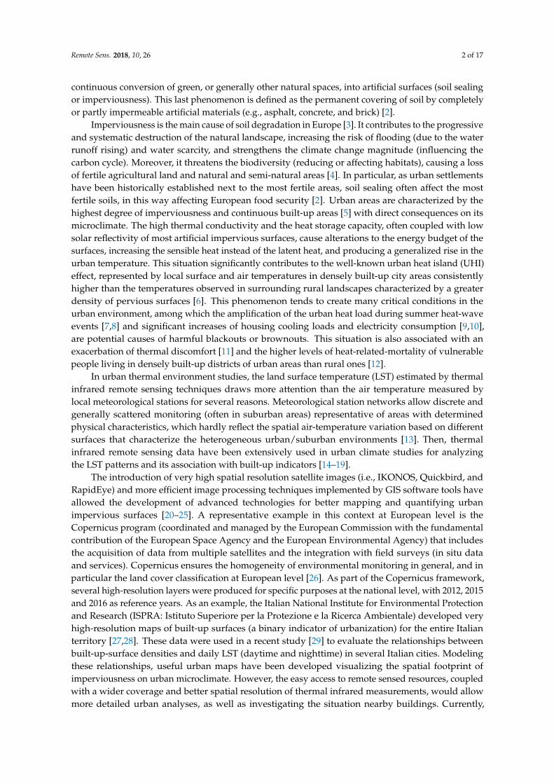
Urban Imperviousness Effects on Summer SurfaceTemperatures Nearby Residential Buildings inDifferent Urban Zones of Parma
Marco Morabito 1,2,*, Alfonso Crisci 1, Teodoro Georgiadis 1, Simone Orlandini 2,3,Michele Munafò 4, Luca Congedo 5 ID , Patrizia Rota 6 and Michele Zazzi 6
1 Institute of Biometeorology, National Research Council, 50145 Florence, Italy; [email protected] (A.C.);[email protected] (T.G.)
2 Centre of Bioclimatology, University of Florence, 50144 Florence, Italy; [email protected] Department of Agrifood Production and Environmental Sciences, University of Florence,
50144 Florence, Italy4 Italian National Institute for Environmental Protection and Research (ISPRA), 00144 Rome, Italy;
[email protected] Department of Architecture and Design (DiAP), Sapienza University of Rome, 00185 Rome, Italy;
[email protected] Department of Engineering and Architecture (DIA), 43124 Parma, Italy; [email protected] (P.R.);
[email protected] (M.Z.)* Correspondence: [email protected]; Tel.: +39-055-522-6041
Received: 25 October 2017; Accepted: 21 December 2017; Published: 24 December 2017
Abstract: Rapid and unplanned urban growth is responsible for the continuous conversion of greenor generally natural spaces into artificial surfaces. The high degree of imperviousness modifiesthe urban microclimate and no studies have quantified its influence on the surface temperature(ST) nearby residential building. This topic represents the aim of this study carried out duringsummer in different urban zones (densely urbanized or park/rural areas) of Parma (Northern Italy).Daytime and nighttime ASTER images, the local urban cartography and the Italian imperviousnessdatabases were used. A reproducible/replicable framework was implemented named “BuildingThermal Functional Area” (BTFA) useful to lead building-proxy thermal analyses by using remotesensing data. For each residential building (n = 8898), the BTFA was assessed and the correspondentASTER-LST value (ST_BTFA) and the imperviousness density were calculated. Both daytime andnighttime ST_BTFA significantly (p < 0.001) increased when high levels of imperviousness densitysurrounded the residential buildings. These relationships were mostly consistent during daytimeand in densely urbanized areas. ST_BTFA differences between urban and park/rural areas werehigher during nighttime (above 1 ◦C) than daytime (about 0.5 ◦C). These results could help to identify“urban thermal Hot-Spots” that would benefit most from mitigation actions.
Keywords: thermal infrared images; urban heat island; soil sealing; city; park; green areas; rural; heat
1. Introduction
Based on the global urban population prospects of the United Nations [1], since 2007, the urbanpopulation is higher than the rural one. In addition, future scenarios suggest that this gap is expectedto continue to grow and about two-thirds of the world’s total population will reside in urban areas by2050 [1]. This pattern is already a reality in Europe, where more than 70% of people live in cities, townsand other urban settlements (generally small cities with fewer than 500,000 inhabitants). Continuousurban land expansion at rates much higher than population growth has led to a massive urban footprinton Europe. The rapid and often uncontrolled and/or unplanned urban growth is responsible for the
Remote Sens. 2018, 10, 26; doi:10.3390/rs10010026 www.mdpi.com/journal/remotesensing
Remote Sens. 2018, 10, 26 2 of 17
continuous conversion of green, or generally other natural spaces, into artificial surfaces (soil sealingor imperviousness). This last phenomenon is defined as the permanent covering of soil by completelyor partly impermeable artificial materials (e.g., asphalt, concrete, and brick) [2].
Imperviousness is the main cause of soil degradation in Europe [3]. It contributes to the progressiveand systematic destruction of the natural landscape, increasing the risk of flooding (due to the waterrunoff rising) and water scarcity, and strengthens the climate change magnitude (influencing thecarbon cycle). Moreover, it threatens the biodiversity (reducing or affecting habitats), causing a lossof fertile agricultural land and natural and semi-natural areas [4]. In particular, as urban settlementshave been historically established next to the most fertile areas, soil sealing often affect the mostfertile soils, in this way affecting European food security [2]. Urban areas are characterized by thehighest degree of imperviousness and continuous built-up areas [5] with direct consequences on itsmicroclimate. The high thermal conductivity and the heat storage capacity, often coupled with lowsolar reflectivity of most artificial impervious surfaces, cause alterations to the energy budget of thesurfaces, increasing the sensible heat instead of the latent heat, and producing a generalized rise in theurban temperature. This situation significantly contributes to the well-known urban heat island (UHI)effect, represented by local surface and air temperatures in densely built-up city areas consistentlyhigher than the temperatures observed in surrounding rural landscapes characterized by a greaterdensity of pervious surfaces [6]. This phenomenon tends to create many critical conditions in theurban environment, among which the amplification of the urban heat load during summer heat-waveevents [7,8] and significant increases of housing cooling loads and electricity consumption [9,10],are potential causes of harmful blackouts or brownouts. This situation is also associated with anexacerbation of thermal discomfort [11] and the higher levels of heat-related-mortality of vulnerablepeople living in densely built-up districts of urban areas than rural ones [12].
In urban thermal environment studies, the land surface temperature (LST) estimated by thermalinfrared remote sensing techniques draws more attention than the air temperature measured bylocal meteorological stations for several reasons. Meteorological station networks allow discrete andgenerally scattered monitoring (often in suburban areas) representative of areas with determinedphysical characteristics, which hardly reflect the spatial air-temperature variation based on differentsurfaces that characterize the heterogeneous urban/suburban environments [13]. Then, thermalinfrared remote sensing data have been extensively used in urban climate studies for analyzingthe LST patterns and its association with built-up indicators [14–19].
The introduction of very high spatial resolution satellite images (i.e., IKONOS, Quickbird, andRapidEye) and more efficient image processing techniques implemented by GIS software tools haveallowed the development of advanced technologies for better mapping and quantifying urbanimpervious surfaces [20–25]. A representative example in this context at European level is theCopernicus program (coordinated and managed by the European Commission with the fundamentalcontribution of the European Space Agency and the European Environmental Agency) that includesthe acquisition of data from multiple satellites and the integration with field surveys (in situ dataand services). Copernicus ensures the homogeneity of environmental monitoring in general, and inparticular the land cover classification at European level [26]. As part of the Copernicus framework,several high-resolution layers were produced for specific purposes at the national level, with 2012, 2015and 2016 as reference years. As an example, the Italian National Institute for Environmental Protectionand Research (ISPRA: Istituto Superiore per la Protezione e la Ricerca Ambientale) developed veryhigh-resolution maps of built-up surfaces (a binary indicator of urbanization) for the entire Italianterritory [27,28]. These data were used in a recent study [29] to evaluate the relationships betweenbuilt-up-surface densities and daily LST (daytime and nighttime) in several Italian cities. Modelingthese relationships, useful urban maps have been developed visualizing the spatial footprint ofimperviousness on urban microclimate. However, the easy access to remote sensed resources, coupledwith a wider coverage and better spatial resolution of thermal infrared measurements, would allowmore detailed urban analyses, as well as investigating the situation nearby buildings. Currently,
Remote Sens. 2018, 10, 26 3 of 17
only rare studies [30] used high-resolution thermal remotely imageries to deal with individualbuilding structures. For this reason, the aim of the present study is to provide a framework,valid for an Italian urban summer context (Parma), able to investigate the relationships betweenthe surface temperature nearby residential buildings, by using high-resolution thermal images(NASA-ASTER), and the surrounding imperviousness density assessed through the high-resolutionItalian built-up-surfaces database provided by ISPRA. This study is based on the hypothesis that,during a generic summer day, the surface temperature nearby a residential building is influenced byits surrounding imperviousness density.
2. Materials and Methods
2.1. Study Area and Summer Climate Characteristics
This study was carried out on the inland city of Parma, a municipality with an area of about260 km2 (small city size), an elevation of 55 m, and almost 200,000 inhabitants (population density740/km2) located in Northern Italy, the western part of the Emilia Romagna region, betweenthe Apennines and the Po Valley. According to the Köppen climate classification [31], Parma ischaracterized by a humid subtropical climate (Cfa). In particular, the summers are hot and sultry,with monthly average maximum temperatures ranging about 24–27 ◦C during September and Juneand 28–30 ◦C during August and July. The monthly average minimum temperatures during summermonths range 14–16 ◦C during September and June and 17–18 ◦C during August and July. Summerdays are often affected by afternoon thunderstorms. The average monthly precipitations duringsummer range from about 50 mm during July (the driest month) to about 70 mm during September.
2.2. Daytime and Nighttime LST
The freely available Advanced Spaceborne Thermal Emission and Reflection Radiometer (ASTER)remote sensing data products [32] were used to estimate daytime and nighttime LST. ASTER is amultispectral imager that was provided by the Japanese Ministry of Economy, Trade and Industry(METI: Tokyo, Japan) for launch on board the National Aeronautics and Space Administration (NASA:Washington, DC, USA) Earth Observing System (EOS) Terra spacecraft in December 1999. ASTERprovides high-resolution images of the planet Earth in 14 different bands of the electromagneticspectrum, ranging from visible to thermal infrared light. In this study, the ASTER Level 1 PrecisionTerrain Corrected Registered At-Sensor Radiance (AST_L1T) data product [33] was used and retrievedfrom the online Data Pool [34], courtesy of the NASA Land Processes Distributed Active Archive Center(LP DAAC: Sioux Falls, SD, USA), USGS/Earth Resources Observation and Science (EROS) Center,Sioux Falls, SD, USA. The AST_L1T data contain calibrated at-sensor radiance, which corresponds withthe ASTER Level 1B (AST_L1B) that has been geometrically corrected, and rotated to a north-up UTMprojection [33]. The thermal infrared (TIR) wavelength band 14 (TIR_Band14: µm 10.950–11.650) withhigh-spatial resolution (90 m resolution), but low–temporal resolution (temporal frequency greaterthan 15 days), was used for LST estimation. In particular, the LST estimation was carried out by usinga customized R code (aster_layer_calc.r) available in the section “code” of the public repository of theGitHub platform [35] that contains all data and codes developed for this work. The procedure is basedon the work described at the NASA Earthdata work repository [36]. This code performs extraction andconversion of TIR_Band14 from original ASTER files and calculates the AST_L1T (spectral radiance atthe sensor’s aperture, Lλ) by using the relation:
Lλ = (DN − 1) × UCC, (1)
where DN is the digital number of data stored in image’s arrays; and UCC is the unit conversioncoefficient (W m−2 sr−1 µm−1).
Remote Sens. 2018, 10, 26 4 of 17
Hence, the code provides an estimation of brightness temperatures (TB):
TB = K2/ ln (K1/Lλ + 1), (2)
where K2 (1.273 × 10³) and K1 (6.464 × 10²) are the band-specific thermal conversion constants.Finally, LST was estimated thanks to a weighted Planck function:
LST = TB/[1 + (λ × TB/c2) × ln (ε), (3)
where λ is the wavelength of emitted radiance (band 14); ε is the surface emissivity dimensionless (inthis study 0.95 and 0.90); and c2 is obtained by the following equation:
c2 = h × c/s = 1.4388 × 10⁻² m K = 14,388 µm K, (4)
where h is Planck’s constant (6.626 × 10⁻³⁴ J s); c is the speed of light (2.998 × 10⁸ m/s); and s is theBoltzmann constant (1.38 × 10⁻²³ J K−1).
The procedure of LST estimation used in this study follows the same scheme adopted in QGISSemi-Automatic Classification Plugin [37]. Most roofs of residential buildings in the city of Parmaare characterized by red rough bricks and, for this reason, a general emissivity value of 0.95 wasconsidered (analyses were also carried out with an average emissivity value of 0.90).
In this study, six clear-sky ASTER images (four daytime and two nighttime images) clearlycovering the city of Parma were acquired during the summer months (Table 1).
Table 1. The list of dates of the ASTER images selected and the corresponding daily meteorologicalcharacteristics of Parma.
Date(Day/Month/Year) Time of Day Time (h:min:s) Meteorological Characteristics of Parma
25 June 2016 Nighttime 21:18:34 Tmax 34 ◦C; Tmin 23 ◦C; RH 54%; Windspeed 5 km/h; Clear sky; No precipitation
30 June 2015 Daytime 10:17:20 Tmax 30 ◦C; Tmin 20 ◦C; RH 54%; Windspeed 7 km/h; Clear sky; No precipitation
25 July 2010 Daytime 10:22:13 Tmax 29 ◦C; Tmin 15 ◦C; RH 42%; Windspeed 6 km/h; Clear sky; No precipitation
3 August 2016 Daytime 10:17:00 Tmax 32 ◦C; Tmin 20 ◦C; RH 53%; Windspeed 6 km/h; Clear sky; No precipitation
26 August 2015 Nighttime 21:18:34 Tmax 29 ◦C; Tmin 17 ◦C; RH 63%; Windspeed 4 km/h; Clear sky; No precipitation
6 September 2014 Daytime 10:22:52 Tmax 28 ◦C; Tmin 18 ◦C; RH 68%; Windspeed 5 km/h; Clear sky; No precipitation
Tmax and Tmin are the daily maximum and minimum temperatures, respectively; RH is the relative humidity.
2.3. Urban Imperviousness
The very high-resolution (10 m) urban imperviousness (or built-up-surface) indicator usedin this study was provided and made freely available by ISPRA (Italian National Institute forEnvironmental Protection and Research) [38]. This spatial dataset covers the entire Italian territory andwas developed merging information obtained by using RapidEye images and the Sentinel-2A satellitedata coverages available for the year 2015, improving the previous national high-resolution (20 m)imperviousness cartography of the Copernicus Program [26]. In addition, the overall accuracy of thedata and the image classification system was verified by using the vector information coming fromOpenStreetMap data [28], the main worldwide collaborative project for free mapping. All informationachieved on the spatial degree of imperviousness are finally classified into a binary product by
Remote Sens. 2018, 10, 26 5 of 17
applying a threshold value of 30% following a simple rule [39]: 0–29% = pervious surface (value = 0);30–100% = impervious surface (value = 1). The areas classified as imperviousness include buildings,sheds, transport, industrial and commercial areas, recreational parks, construction sites, roads, railways,railway locations, permanent greenhouse, mining areas, landfills, and other infrastructures. Thevalidation of this binary environmental indicator has been carried out through a comparison withthe monitoring points of the national and regional impervious surfaces network, revealing an overallaccuracy greater than 95% [28]. Urban imperviousness was extracted for the municipality of Parma,one of the Italian municipalities with the highest imperviousness values (only after Rome, Milan, Turin,Naples, Venice, Ravenna and Palermo). In particular, Parma has about 23% of its municipal territory(6104 ha) classified as impervious [28]. The spatial extent of the work was provided by the ItalianNational Institute of Statistics (ISTAT) data using Parma’s administrative boundaries [40]. Residentialbuilding’s data of Parma were provided by the Emilia Romagna regional geoportal and in particular,the regional topographic database [41].
2.4. Study Framework and Statistical Analyses
Statistical analyses were carried out using IBM SPSS software [42] and open source R environmentsoftware [43] with specific packages for spatial data processing and mapping tasks [44–46].
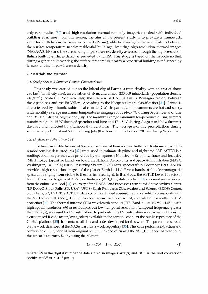
The analyses are focused on residential buildings located in the municipality of Parma, alsoaccounting for urban zones, such as typical urban (densely built-up) and park/rural areas. Urbanzones were identified using the local cartography provided by Parma’s municipal territorial planningsector (Settore Pianificazione Territoriale del Comune di Parma). Of the total 10,444 residentialbuildings available, 15.3% of data were excluded for missing or incomplete information and 8898(84.7%) were included in the study (Figure 1).
Remote Sens. 2017, 10, 26 5 of 18
Remote Sens. 2017, 10, 26; doi:10.3390/rs10010026 www.mdpi.com/journal/remotesensing
revealing an overall accuracy greater than 95% [28]. Urban imperviousness was extracted for the
municipality of Parma, one of the Italian municipalities with the highest imperviousness values
(only after Rome, Milan, Turin, Naples, Venice, Ravenna and Palermo). In particular, Parma has
about 23% of its municipal territory (6104 ha) classified as impervious [28]. The spatial extent of the
work was provided by the Italian National Institute of Statistics (ISTAT) data using Parma’s
administrative boundaries [40]. Residential building’s data of Parma were provided by the Emilia
Romagna regional geoportal and in particular, the regional topographic database [41].
2.4. Study Framework and Statistical Analyses
Statistical analyses were carried out using IBM SPSS software [42] and open source R
environment software [43] with specific packages for spatial data processing and mapping tasks [44–46].
The analyses are focused on residential buildings located in the municipality of Parma, also
accounting for urban zones, such as typical urban (densely built-up) and park/rural areas. Urban
zones were identified using the local cartography provided by Parma’s municipal territorial planning
sector (Settore Pianificazione Territoriale del Comune di Parma). Of the total 10,444 residential
buildings available, 15.3% of data were excluded for missing or incomplete information and 8898
(84.7%) were included in the study (Figure 1).
Figure 1. Map of residential buildings (black polygons) located in the city center of Parma. Impervious
and pervious surfaces are indicated in grey and white, respectively.
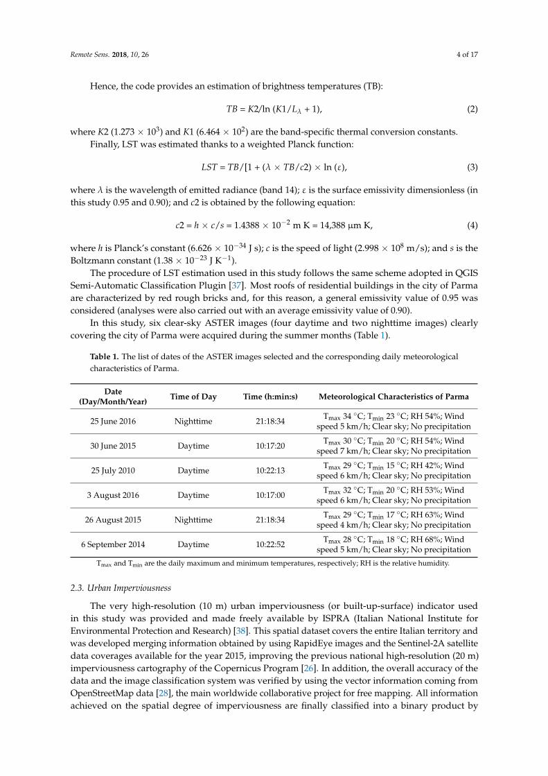
As the ASTER-LST spatial resolution (90 m × 90 m) (red squares in Figure 2) is not suitable for
measuring exactly the building surface temperature, we have assumed that an area around each
residential building exists, defined as “Building Thermal Functional Area” (BTFA), useful to lead
building-proxy thermal analyses by using ASTER information sources. The BTFA, in function to its
characteristics (i.e., the imperviousness density), could affect the building thermal status in a
proportional way. The BTFA was assessed by using a circular model where its center was the building
centroid (Figure 2): the radius considered was of about 56 m, in this way defining an area (BTFA) of
about 1 ha. The choice of 1 ha was based on the unit used to measure the area of a farmland and
building land as reported in the European Directive 80/181/EEC [47]. For each BTFA assessed, the
correspondent ASTER-LST value (ST_BTFA) was extracted by using the coordinates of the BTFA
Figure 1. Map of residential buildings (black polygons) located in the city center of Parma. Imperviousand pervious surfaces are indicated in grey and white, respectively.
As the ASTER-LST spatial resolution (90 m × 90 m) (red squares in Figure 2) is not suitablefor measuring exactly the building surface temperature, we have assumed that an area around eachresidential building exists, defined as “Building Thermal Functional Area” (BTFA), useful to lead
Remote Sens. 2018, 10, 26 6 of 17
building-proxy thermal analyses by using ASTER information sources. The BTFA, in function toits characteristics (i.e., the imperviousness density), could affect the building thermal status in aproportional way. The BTFA was assessed by using a circular model where its center was the buildingcentroid (Figure 2): the radius considered was of about 56 m, in this way defining an area (BTFA)of about 1 ha. The choice of 1 ha was based on the unit used to measure the area of a farmland andbuilding land as reported in the European Directive 80/181/EEC [47]. For each BTFA assessed, thecorrespondent ASTER-LST value (ST_BTFA) was extracted by using the coordinates of the BTFA centerthat also corresponds to the residential building centroid (Figure 2). For each BTFA, the imperviousnessdensity value (ID) was assessed (Figure 2).
Remote Sens. 2017, 10, 26 6 of 18
Remote Sens. 2017, 10, 26; doi:10.3390/rs10010026 www.mdpi.com/journal/remotesensing
center that also corresponds to the residential building centroid (Figure 2). For each BTFA, the
imperviousness density value (ID) was assessed (Figure 2).
Figure 2. Building Thermal Functional Area (BTFA) framework. The black circle delimits the 1-ha
residential BTFA. The blue point is the BTFA center (building centroid). Red squares represent the
ASTER-LST pixels (90 m resolution). Impervious and pervious surfaces (10 m resolution) are
indicated by grey and white colors respectively.
Then, the extracted daytime and nighttime ST_BTFA values were classified by using the
correspondent ID value into five ID groups: (1) very low ID ≤ 20%; (2) low 20% < ID ≤ 40%; (3)
moderate 40% < ID ≤ 60%; (4) high 60% < ID ≤ 80%; and (5) very high ID > 80%. In this way, the
average ST_BTFA for each ID group was calculated and significant ST_BTFA differences were
investigated through nonparametric procedures. This choice was based on the fact that the normal
distribution assumption of the ST_BTFA residuals was not always satisfied. The Kruskal–Wallis test
[48] is a robust equivalent of the one-way analysis of variance (ANOVA) and it was used to compare
the ST_BTFA ranks among the five ID independent groups. The Mann–Whitney U test [49] is the
equivalent of the t-test and it was used to lead a twice-comparison of ST_BTFA medians on ID
independent groups following a multi-comparison scheme.
Preliminary plotting analyses were carried out investigating the relationships between daytime
and nighttime ST_BTFA and ID groups for each available ASTER image.
Subsequently, detailed descriptive and boxplot analyses investigated these relationships in
typical densely urbanized and park/rural areas of the Parma municipality with the aim to evaluate if
different urban zones play a role as confounder.
Data and code functions developed for this work are available in the public repository on the
GitHub platform [35].
Figure 2. Building Thermal Functional Area (BTFA) framework. The black circle delimits the 1-haresidential BTFA. The blue point is the BTFA center (building centroid). Red squares represent theASTER-LST pixels (90 m resolution). Impervious and pervious surfaces (10 m resolution) are indicatedby grey and white colors respectively.
Then, the extracted daytime and nighttime ST_BTFA values were classified by using thecorrespondent ID value into five ID groups: (1) very low ID ≤ 20%; (2) low 20% < ID ≤ 40%;(3) moderate 40% < ID ≤ 60%; (4) high 60% < ID ≤ 80%; and (5) very high ID > 80%. In this way,the average ST_BTFA for each ID group was calculated and significant ST_BTFA differences wereinvestigated through nonparametric procedures. This choice was based on the fact that the normaldistribution assumption of the ST_BTFA residuals was not always satisfied. The Kruskal–Wallistest [48] is a robust equivalent of the one-way analysis of variance (ANOVA) and it was used tocompare the ST_BTFA ranks among the five ID independent groups. The Mann–Whitney U test [49]is the equivalent of the t-test and it was used to lead a twice-comparison of ST_BTFA medians on IDindependent groups following a multi-comparison scheme.
Preliminary plotting analyses were carried out investigating the relationships between daytimeand nighttime ST_BTFA and ID groups for each available ASTER image.
Subsequently, detailed descriptive and boxplot analyses investigated these relationships in typicaldensely urbanized and park/rural areas of the Parma municipality with the aim to evaluate if differenturban zones play a role as confounder.
Remote Sens. 2018, 10, 26 7 of 17
Data and code functions developed for this work are available in the public repository on theGitHub platform [35].
3. Results
3.1. Relationships between Daytime and Nighttime ST_BTFA and Imperviousness Density Groups
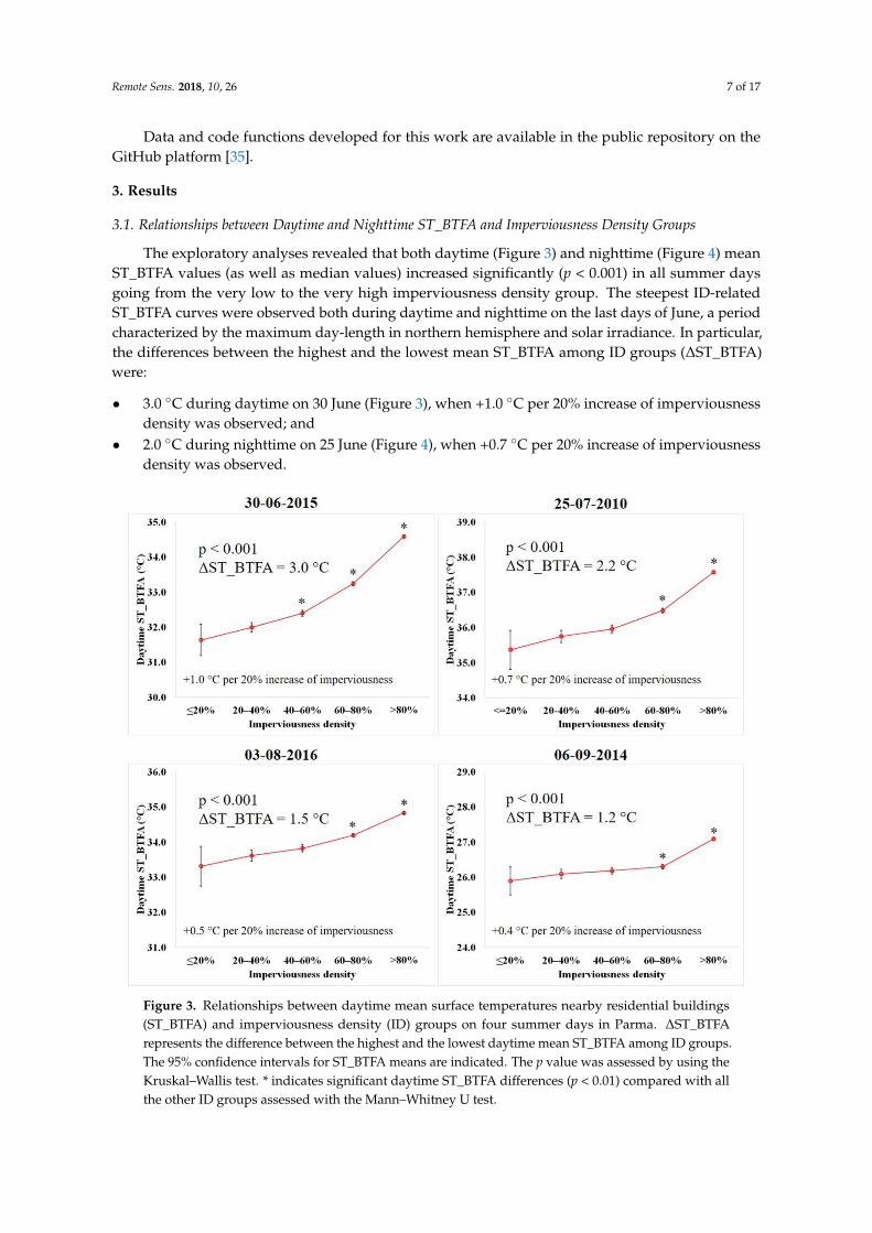
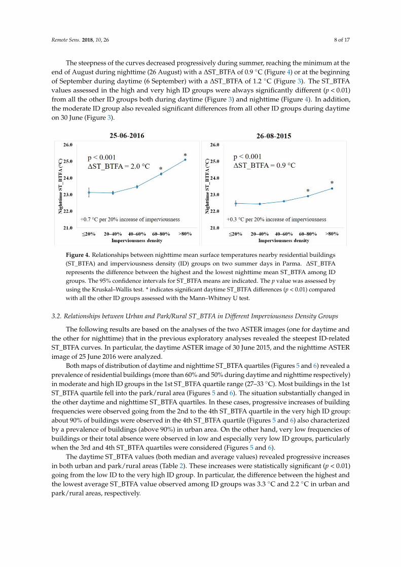
The exploratory analyses revealed that both daytime (Figure 3) and nighttime (Figure 4) meanST_BTFA values (as well as median values) increased significantly (p < 0.001) in all summer daysgoing from the very low to the very high imperviousness density group. The steepest ID-relatedST_BTFA curves were observed both during daytime and nighttime on the last days of June, a periodcharacterized by the maximum day-length in northern hemisphere and solar irradiance. In particular,the differences between the highest and the lowest mean ST_BTFA among ID groups (∆ST_BTFA)were:
• 3.0 ◦C during daytime on 30 June (Figure 3), when +1.0 ◦C per 20% increase of imperviousnessdensity was observed; and
• 2.0 ◦C during nighttime on 25 June (Figure 4), when +0.7 ◦C per 20% increase of imperviousnessdensity was observed.
Remote Sens. 2017, 10, 26 7 of 18
Remote Sens. 2017, 10, 26; doi:10.3390/rs10010026 www.mdpi.com/journal/remotesensing
3. Results
3.1. Relationships between Daytime and Nighttime ST_BTFA and Imperviousness Density Groups
The exploratory analyses revealed that both daytime (Figure 3) and nighttime (Figure 4) mean
ST_BTFA values (as well as median values) increased significantly (p < 0.001) in all summer days
going from the very low to the very high imperviousness density group. The steepest ID-related
ST_BTFA curves were observed both during daytime and nighttime on the last days of June, a period
characterized by the maximum day-length in northern hemisphere and solar irradiance. In particular,
the differences between the highest and the lowest mean ST_BTFA among ID groups (ΔST_BTFA)
were:
3.0 °C during daytime on 30 June (Figure 3), when +1.0 °C per 20% increase of imperviousness
density was observed; and
2.0 °C during nighttime on 25 June (Figure 4), when +0.7 °C per 20% increase of imperviousness
density was observed.
Figure 3. Relationships between daytime mean surface temperatures nearby residential buildings
(ST_BTFA) and imperviousness density (ID) groups on four summer days in Parma. ΔST_BTFA
represents the difference between the highest and the lowest daytime mean ST_BTFA among ID
groups. The 95% confidence intervals for ST_BTFA means are indicated. The p value was assessed by
using the Kruskal–Wallis test. * indicates significant daytime ST_BTFA differences (p < 0.01) compared
with all the other ID groups assessed with the Mann–Whitney U test.
The steepness of the curves decreased progressively during summer, reaching the minimum at
the end of August during nighttime (26 August) with a ΔST_BTFA of 0.9 °C (Figure 4) or at the
beginning of September during daytime (6 September) with a ΔST_BTFA of 1.2 °C (Figure 3). The
Figure 3. Relationships between daytime mean surface temperatures nearby residential buildings(ST_BTFA) and imperviousness density (ID) groups on four summer days in Parma. ∆ST_BTFArepresents the difference between the highest and the lowest daytime mean ST_BTFA among ID groups.The 95% confidence intervals for ST_BTFA means are indicated. The p value was assessed by using theKruskal–Wallis test. * indicates significant daytime ST_BTFA differences (p < 0.01) compared with allthe other ID groups assessed with the Mann–Whitney U test.
Remote Sens. 2018, 10, 26 8 of 17
The steepness of the curves decreased progressively during summer, reaching the minimum at theend of August during nighttime (26 August) with a ∆ST_BTFA of 0.9 ◦C (Figure 4) or at the beginningof September during daytime (6 September) with a ∆ST_BTFA of 1.2 ◦C (Figure 3). The ST_BTFAvalues assessed in the high and very high ID groups were always significantly different (p < 0.01)from all the other ID groups both during daytime (Figure 3) and nighttime (Figure 4). In addition,the moderate ID group also revealed significant differences from all other ID groups during daytimeon 30 June (Figure 3).
Remote Sens. 2017, 10, 26 8 of 18
Remote Sens. 2017, 10, 26; doi:10.3390/rs10010026 www.mdpi.com/journal/remotesensing
ST_BTFA values assessed in the high and very high ID groups were always significantly
different (p < 0.01) from all the other ID groups both during daytime (Figure 3) and nighttime (Figure 4).
In addition, the moderate ID group also revealed significant differences from all other ID groups
during daytime on 30 June (Figure 3).
Figure 4. Relationships between nighttime mean surface temperatures nearby residential buildings
(ST_BTFA) and imperviousness density (ID) groups on two summer days in Parma. ΔST_BTFA
represents the difference between the highest and the lowest nighttime mean ST_BTFA among ID
groups. The 95% confidence intervals for ST_BTFA means are indicated. The p value was assessed by
using the Kruskal–Wallis test. * indicates significant daytime ST_BTFA differences (p < 0.01) compared
with all the other ID groups assessed with the Mann–Whitney U test.
3.2. Relationships between Urban and Park/Rural ST_BTFA in Different Imperviousness Density Groups
The following results are based on the analyses of the two ASTER images (one for daytime and
the other for nighttime) that in the previous exploratory analyses revealed the steepest ID-related
ST_BTFA curves. In particular, the daytime ASTER image of 30 June 2015, and the nighttime ASTER
image of 25 June 2016 were analyzed.
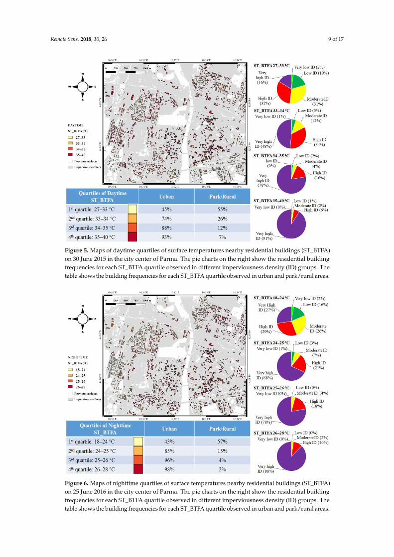
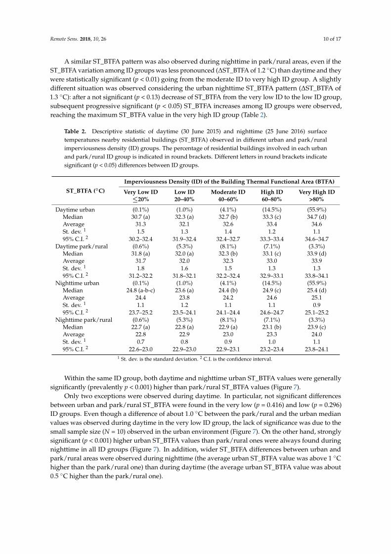
Both maps of distribution of daytime and nighttime ST_BTFA quartiles (Figures 5 and 6)
revealed a prevalence of residential buildings (more than 60% and 50% during daytime and nighttime
respectively) in moderate and high ID groups in the 1st ST_BTFA quartile range (27–33 °C). Most
buildings in the 1st ST_BTFA quartile fell into the park/rural area (Figures 5 and 6). The situation
substantially changed in the other daytime and nighttime ST_BTFA quartiles. In these cases,
progressive increases of building frequencies were observed going from the 2nd to the 4th ST_BTFA
quartile in the very high ID group: about 90% of buildings were observed in the 4th ST_BTFA quartile
(Figures 5 and 6) also characterized by a prevalence of buildings (above 90%) in urban area. On the
other hand, very low frequencies of buildings or their total absence were observed in low and
especially very low ID groups, particularly when the 3rd and 4th ST_BTFA quartiles were considered
(Figures 5 and 6).
The daytime ST_BTFA values (both median and average values) revealed progressive increases
in both urban and park/rural areas (Table 2). These increases were statistically significant (p < 0.01)
going from the low ID to the very high ID group. In particular, the difference between the highest
and the lowest average ST_BTFA value observed among ID groups was 3.3 °C and 2.2 °C in urban
and park/rural areas, respectively.
A similar ST_BTFA pattern was also observed during nighttime in park/rural areas, even if the
ST_BTFA variation among ID groups was less pronounced (ΔST_BTFA of 1.2 °C) than daytime and
they were statistically significant (p < 0.01) going from the moderate ID to very high ID group. A
slightly different situation was observed considering the urban nighttime ST_BTFA pattern
(ΔST_BTFA of 1.3 °C): after a not significant (p < 0.13) decrease of ST_BTFA from the very low ID to
Figure 4. Relationships between nighttime mean surface temperatures nearby residential buildings(ST_BTFA) and imperviousness density (ID) groups on two summer days in Parma. ∆ST_BTFArepresents the difference between the highest and the lowest nighttime mean ST_BTFA among IDgroups. The 95% confidence intervals for ST_BTFA means are indicated. The p value was assessed byusing the Kruskal–Wallis test. * indicates significant daytime ST_BTFA differences (p < 0.01) comparedwith all the other ID groups assessed with the Mann–Whitney U test.
3.2. Relationships between Urban and Park/Rural ST_BTFA in Different Imperviousness Density Groups
The following results are based on the analyses of the two ASTER images (one for daytime andthe other for nighttime) that in the previous exploratory analyses revealed the steepest ID-relatedST_BTFA curves. In particular, the daytime ASTER image of 30 June 2015, and the nighttime ASTERimage of 25 June 2016 were analyzed.
Both maps of distribution of daytime and nighttime ST_BTFA quartiles (Figures 5 and 6) revealed aprevalence of residential buildings (more than 60% and 50% during daytime and nighttime respectively)in moderate and high ID groups in the 1st ST_BTFA quartile range (27–33 ◦C). Most buildings in the 1stST_BTFA quartile fell into the park/rural area (Figures 5 and 6). The situation substantially changed inthe other daytime and nighttime ST_BTFA quartiles. In these cases, progressive increases of buildingfrequencies were observed going from the 2nd to the 4th ST_BTFA quartile in the very high ID group:about 90% of buildings were observed in the 4th ST_BTFA quartile (Figures 5 and 6) also characterizedby a prevalence of buildings (above 90%) in urban area. On the other hand, very low frequencies ofbuildings or their total absence were observed in low and especially very low ID groups, particularlywhen the 3rd and 4th ST_BTFA quartiles were considered (Figures 5 and 6).
The daytime ST_BTFA values (both median and average values) revealed progressive increasesin both urban and park/rural areas (Table 2). These increases were statistically significant (p < 0.01)going from the low ID to the very high ID group. In particular, the difference between the highest andthe lowest average ST_BTFA value observed among ID groups was 3.3 ◦C and 2.2 ◦C in urban andpark/rural areas, respectively.
Remote Sens. 2018, 10, 26 9 of 17
Remote Sens. 2017, 10, 26 9 of 18
Remote Sens. 2017, 10, 26; doi:10.3390/rs10010026 www.mdpi.com/journal/remotesensing
the low ID group, subsequent progressive significant (p < 0.05) ST_BTFA increases among ID groups
were observed, reaching the maximum ST_BTFA value in the very high ID group (Table 2).
Figure 5. Maps of daytime quartiles of surface temperatures nearby residential buildings (ST_BTFA) on
30 June 2015 in the city center of Parma. The pie charts on the right show the residential building
frequencies for each ST_BTFA quartile observed in different imperviousness density (ID) groups. The
table shows the building frequencies for each ST_BTFA quartile observed in urban and park/rural areas.
Figure 5. Maps of daytime quartiles of surface temperatures nearby residential buildings (ST_BTFA)on 30 June 2015 in the city center of Parma. The pie charts on the right show the residential buildingfrequencies for each ST_BTFA quartile observed in different imperviousness density (ID) groups. Thetable shows the building frequencies for each ST_BTFA quartile observed in urban and park/rural areas.Remote Sens. 2017, 10, 26 10 of 18
Remote Sens. 2017, 10, 26; doi:10.3390/rs10010026 www.mdpi.com/journal/remotesensing
Figure 6. Maps of nighttime quartiles of surface temperatures nearby residential buildings (ST_BTFA)
on 25 June 2016 in the city center of Parma. The pie charts on the right show the residential building
frequencies for each ST_BTFA quartile observed in different imperviousness density (ID) groups. The
table shows the building frequencies for each ST_BTFA quartile observed in urban and park/rural areas.
Table 2. Descriptive statistic of daytime (30 June 2015) and nighttime (25 June 2016) surface
temperatures nearby residential buildings (ST_BTFA) observed in different urban and park/rural
imperviousness density (ID) groups. The percentage of residential buildings involved in each urban
and park/rural ID group is indicated in round brackets. Different letters in round brackets indicate
significant (p < 0.05) differences between ID groups.
ST_BTFA (°C)
Imperviousness Density (ID) of the Building Thermal Functional Area (BTFA)
Very Low ID
≤20%
Low ID
20–40%
Moderate ID
40–60%
High ID
60–80%
Very High ID
>80%
Daytime urban (0.1%) (1.0%) (4.1%) (14.5%) (55.9%)
Median 30.7 (a) 32.3 (a) 32.7 (b) 33.3 (c) 34.7 (d)
Average 31.3 32.1 32.6 33.4 34.6
St. dev. 1 1.5 1.3 1.4 1.2 1.1
95% C.I. 2 30.2–32.4 31.9–32.4 32.4–32.7 33.3–33.4 34.6–34.7
Daytime park/rural (0.6%) (5.3%) (8.1%) (7.1%) (3.3%)
Median 31.8 (a) 32.0 (a) 32.3 (b) 33.1 (c) 33.9 (d)
Average 31.7 32.0 32.3 33.0 33.9
St. dev. 1 1.8 1.6 1.5 1.3 1.3
95% C.I. 2 31.2–32.2 31.8–32.1 32.2–32.4 32.9–33.1 33.8–34.1
Nighttime urban (0.1%) (1.0%) (4.1%) (14.5%) (55.9%)
Median 24.8 (a-b-c) 23.6 (a) 24.4 (b) 24.9 (c) 25.4 (d)
Average 24.4 23.8 24.2 24.6 25.1
St. dev. 1 1.1 1.2 1.1 1.1 0.9
95% C.I. 2 23.7–25.2 23.5–24.1 24.1–24.4 24.6–24.7 25.1–25.2
Nighttime
park/rural (0.6%) (5.3%) (8.1%) (7.1%) (3.3%)
Figure 6. Maps of nighttime quartiles of surface temperatures nearby residential buildings (ST_BTFA)on 25 June 2016 in the city center of Parma. The pie charts on the right show the residential buildingfrequencies for each ST_BTFA quartile observed in different imperviousness density (ID) groups. Thetable shows the building frequencies for each ST_BTFA quartile observed in urban and park/rural areas.
Remote Sens. 2018, 10, 26 10 of 17
A similar ST_BTFA pattern was also observed during nighttime in park/rural areas, even if theST_BTFA variation among ID groups was less pronounced (∆ST_BTFA of 1.2 ◦C) than daytime and theywere statistically significant (p < 0.01) going from the moderate ID to very high ID group. A slightlydifferent situation was observed considering the urban nighttime ST_BTFA pattern (∆ST_BTFA of1.3 ◦C): after a not significant (p < 0.13) decrease of ST_BTFA from the very low ID to the low ID group,subsequent progressive significant (p < 0.05) ST_BTFA increases among ID groups were observed,reaching the maximum ST_BTFA value in the very high ID group (Table 2).
Table 2. Descriptive statistic of daytime (30 June 2015) and nighttime (25 June 2016) surfacetemperatures nearby residential buildings (ST_BTFA) observed in different urban and park/ruralimperviousness density (ID) groups. The percentage of residential buildings involved in each urbanand park/rural ID group is indicated in round brackets. Different letters in round brackets indicatesignificant (p < 0.05) differences between ID groups.
ST_BTFA (◦C)
Imperviousness Density (ID) of the Building Thermal Functional Area (BTFA)
Very Low ID≤20%
Low ID20–40%
Moderate ID40–60%
High ID60–80%
Very High ID>80%
Daytime urban (0.1%) (1.0%) (4.1%) (14.5%) (55.9%)Median 30.7 (a) 32.3 (a) 32.7 (b) 33.3 (c) 34.7 (d)Average 31.3 32.1 32.6 33.4 34.6St. dev. 1 1.5 1.3 1.4 1.2 1.195% C.I. 2 30.2–32.4 31.9–32.4 32.4–32.7 33.3–33.4 34.6–34.7
Daytime park/rural (0.6%) (5.3%) (8.1%) (7.1%) (3.3%)Median 31.8 (a) 32.0 (a) 32.3 (b) 33.1 (c) 33.9 (d)Average 31.7 32.0 32.3 33.0 33.9St. dev. 1 1.8 1.6 1.5 1.3 1.395% C.I. 2 31.2–32.2 31.8–32.1 32.2–32.4 32.9–33.1 33.8–34.1
Nighttime urban (0.1%) (1.0%) (4.1%) (14.5%) (55.9%)Median 24.8 (a-b-c) 23.6 (a) 24.4 (b) 24.9 (c) 25.4 (d)Average 24.4 23.8 24.2 24.6 25.1St. dev. 1 1.1 1.2 1.1 1.1 0.995% C.I. 2 23.7–25.2 23.5–24.1 24.1–24.4 24.6–24.7 25.1–25.2
Nighttime park/rural (0.6%) (5.3%) (8.1%) (7.1%) (3.3%)Median 22.7 (a) 22.8 (a) 22.9 (a) 23.1 (b) 23.9 (c)Average 22.8 22.9 23.0 23.3 24.0St. dev. 1 0.7 0.8 0.9 1.0 1.195% C.I. 2 22.6–23.0 22.9–23.0 22.9–23.1 23.2–23.4 23.8–24.1
1 St. dev. is the standard deviation. 2 C.I. is the confidence interval.
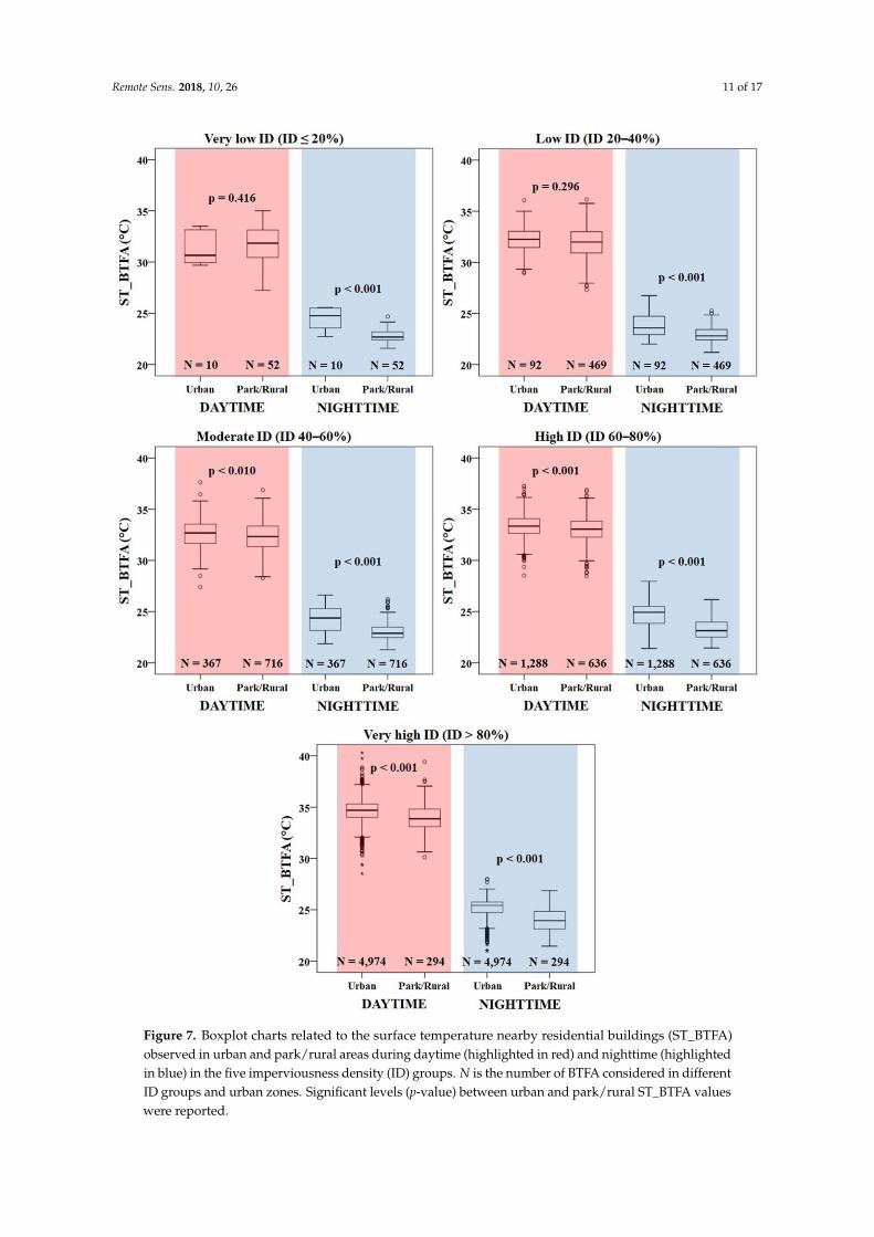
Within the same ID group, both daytime and nighttime urban ST_BTFA values were generallysignificantly (prevalently p < 0.001) higher than park/rural ST_BTFA values (Figure 7).
Only two exceptions were observed during daytime. In particular, not significant differencesbetween urban and park/rural ST_BTFA were found in the very low (p = 0.416) and low (p = 0.296)ID groups. Even though a difference of about 1.0 ◦C between the park/rural and the urban medianvalues was observed during daytime in the very low ID group, the lack of significance was due to thesmall sample size (N = 10) observed in the urban environment (Figure 7). On the other hand, stronglysignificant (p < 0.001) higher urban ST_BTFA values than park/rural ones were always found duringnighttime in all ID groups (Figure 7). In addition, wider ST_BTFA differences between urban andpark/rural areas were observed during nighttime (the average urban ST_BTFA value was above 1 ◦Chigher than the park/rural one) than during daytime (the average urban ST_BTFA value was about0.5 ◦C higher than the park/rural one).
Remote Sens. 2018, 10, 26 11 of 17Remote Sens. 2017, 10, 26 12 of 18
Remote Sens. 2017, 10, 26; doi:10.3390/rs10010026 www.mdpi.com/journal/remotesensing
Figure 7. Boxplot charts related to the surface temperature nearby residential buildings (ST_BTFA)
observed in urban and park/rural areas during daytime (highlighted in red) and nighttime
(highlighted in blue) in the five imperviousness density (ID) groups. N is the number of BTFA
considered in different ID groups and urban zones. Significant levels (p-value) between urban and
park/rural ST_BTFA values were reported.
Figure 7. Boxplot charts related to the surface temperature nearby residential buildings (ST_BTFA)observed in urban and park/rural areas during daytime (highlighted in red) and nighttime (highlightedin blue) in the five imperviousness density (ID) groups. N is the number of BTFA considered in differentID groups and urban zones. Significant levels (p-value) between urban and park/rural ST_BTFA valueswere reported.
Remote Sens. 2018, 10, 26 12 of 17
4. Discussion
Close to two thirds of Europe’s urban dwellers reside in small urban places (in settlements withfewer than 500,000 inhabitants) [1], which therefore represent sensitive environments towards whichto pay much attention. For this reason, this study was focused on a little Italian municipality (Parma)with about 200,000 inhabitants and with a very high urban imperviousness degree: almost a quarter ofits municipal territory is classified as imperviousness [28].
The main findings of this study can be summarized as follows:
1. The rise of ST_BTFA observed increasing the ID was mostly more consistent during daytime thannighttime, and in densely urban zones than park/rural zones:
a. +1.0 ◦C and +0.7 ◦C per 20% increase of imperviousness were observed during daytimeand nighttime respectively at the end of June;
b. daytime ∆ST_BTFA among ID groups was 3.3 ◦C in urban areas and 2.2 ◦C in park/ruralareas; and
c. nighttime ∆ST_BTFA among ID groups was 1.3 ◦C in urban areas and 1.2 ◦C inpark/rural areas.
2. Within the same ID group, ST_BTFA differences between urban and park/rural areas were higherduring nighttime (above 1 ◦C) than during daytime (about 0.5 ◦C).
3. The strongest ID-related ST_BTFA increases were observed on days characterized by themaximum summer day-length and solar radiative load (days at the end of June).
While it is well understood that imperviousness increases surface temperatures [17,50,51] and thatthe impervious percentage accounts for most of the LST variation in urban areas [15,18,52,53], very littleis known about the situation nearby residential buildings, especially when different urban zones areconsidered. The knowledge of how the surface temperature nearby residential buildings varies basedon the surrounding imperviousness density is very important information that assumes further interestin this study where significant ST_BTFA differences between densely urban and park/rural areas wereobserved, also revealing different dynamics during daytime and nighttime. This finding supportsresults coming from previous studies where the influence of urban parks and greenspaces as coolingelements, or less warming elements, can extend several hundred meters beyond their boundaries intothe built-up area [54,55]. In a recent study [19] carried out in a Chinese city, where a dramatic expansionof the urbanized area was observed in the last few years, the authors found that the urban green spaceswere cooler, especially thanks to evapotranspiration, than the surrounding built-up areas, reducingtheir summer LST by several degrees. This information supports previous studies, which have shownnegative correlation between the percentage of green vegetation and LST [53,56]. In addition, our studyalso revealed greatest ST_BTFA differences (above 1 ◦C) between urban and park/rural areas duringnighttime. This means that the cooling effect of green areas on surface temperatures nearby residentialbuildings is greater during nighttime, when the direct downward solar radiation contribution is null.This is in agreement with the fact that the UHI is a typically nighttime phenomenon [53,57] when theradiation stored during the day in the densely built-up areas is released into the atmosphere duringthe night [29]. These findings are especially useful in a country such as Italy where frequent and oftenintense heat waves occur during summer, and a general increased earliness in the occurrence of themost critical heat waves was observed at the end of June [58], when day-length is a risk factor withoften devastating effects for the general population and especially the most vulnerable subjects [59,60].
In the present study, the reliability of the high spatial resolution imagery has allowed obtainingdetailed information on imperviousness-related surface temperature nearby residential buildings. Thisinformation is of particular importance in light of the fact that rooftops are the major impervioussurfaces in the urban residential environment [30] and asphalt surfaces, generally located nearbuildings, are the land cover class that exacerbates extreme heat [53]. Our findings partly confirmswhat has already been highlighted in the few previous studies that have dealt with similar issues. In a
Remote Sens. 2018, 10, 26 13 of 17
study carried out in an American city (Phoenix) with a subtropical desert climate [61], the authorsfound that the presence of buildings does not explain much of the variation in LST. However, themajority of buildings in Phoenix are composed of bright materials with light color rooftops, whichreflect most of incoming solar radiation and retain low amount of heat. On the other hand, in ourstudy, most residential building roofs are characterized by red rough bricks, which reflect much lesssolar radiation and retain more heat. This last observation is in agreement with findings from anotherAmerican study carried out in Baltimore [62], where most building are constructed with dark-coloredrooftops, and also suggest that relationships between imperviousness density and surface temperatureof buildings could vary significantly from city to city and within cities also based on the rooftopcharacteristics [61].
The strongest association between ST_BTFA and the surrounding imperviousness densityparticularly evident in this study on days characterized by the maximum summer solar radiativeload enhanced the sunlight contribution to the thermal building balance especially during the hottestperiod of the year. This result supports the finding concerning the higher ID-related ST_BTFA increaseobserved during daytime than nighttime. This is also in agreement with Zhao et al. [30] who revealedthat rooftop characteristics explain over 30% of daytime rooftop surface temperature variations andslightly more than 17% of nighttime temperatures. The authors also suggested that the direct solarinsolation rather than heat retention of rooftop materials explained well the observed temperaturevariations. In addition, other authors [53] also revealed that greater residential building fractionincrease daytime surface temperatures with insignificant nighttime impact.
The possibility to use thermal infrared images with very high spatial resolutions in this andseveral previous studies have allowed for better understanding of microclimate patterns at the urbanlevel, providing useful information for local authorities, land-use decision makers, and urban planners.However, findings from this study are not generalizable and are only valid for inland cities with similarclimate and urban characteristics, such as the city size, rooftop characteristics, and comparable urbanimperviousness densities. Further studies should investigate these relationships in cities with differentclimate and urban features, also including data related the urban morphology included in the BTFAframework proposed, able to confirm these results or helping to understand other urban microclimatedynamics. The study of the urban thermal impact on sensible elements, such as residential buildings,where people and vulnerable subjects spend most of their time, represents a priority in a contextof global warming. In this way, targeted interventions can be better planned, identifying exactlywhere the critical areas are and providing insights for UHI mitigation’s actions, such as building greeninfrastructures near residential areas (especially trees and shrubs), set up green and cool roofs, andmoreover considering alternative urban design. Each improvement in the spatial knowledge of theurban climate and the behavior of specific urban zones, especially during severe climatic events (suchas heat-waves, wind storms, floods), is important to increment awareness of risk and consequently anovel potential resiliency could be reached. Following this, a next step will also be the development ofa summer heat-related building risk index assessed accounting any census information (at residentialbuilding scale) available and other sociological urban data sources.
5. Conclusions
This fine-scale urban study carried out in a typical small Italian city represents an original effortto provide a reproducible/replicable framework for better understanding the effects of differentimperviousness density levels, during summer days, on surface temperatures nearby residentialbuildings in different urban zones (typical densely urbanized or park/rural areas). It is a practicalexample of how high-resolution thermal infrared remote sensing data can be useful for urban detailedanalyses, as well as investigating the situation nearby single buildings, thus improving knowledgeon urban climate dynamics that regulate the interactions between urban elements, the degree ofimperviousness and thermal surface modifications.
Remote Sens. 2018, 10, 26 14 of 17
This study confirms the hypothesis that, during a summer day, the surface temperature nearby aresidential building is influenced by the surrounding imperviousness degree. In particular, significantST_BTFA increases were observed when impervious density values grew, generating different thermaldynamics during daytime and nighttime in urban and park/rural areas. The highest ST_BTFA valuewas observed in summer days (with higher irradiation and day-length) when very high imperviousnessdensities (>80%) surrounding building favors the formation of particularly critical areas “urban thermalhot-spots” that, also including residential buildings, can create risky conditions above all for thecity dwellers and for most vulnerable people or those not acclimatized to the heat [13]. Virtually,the presence of excessive and continuous impervious surfaces surrounding residential buildings insummer days prevent their heat loss and result in extreme heat conditions, causing what could bedefined as a “building heat stroke”. Fine-scale urban studies represent a major challenge in the nearfuture for better understanding the relationships between microclimate conditions and small areaurban characteristics helpful to improve the UHI mitigation strategies. For individual structures suchas residential buildings, cooler summer conditions due to the effect of nearby parks or any greenspacescan represent reliable UHI mitigation actions addressed to enhance the urban ecosystem and favoringa range of human health benefits. This is a priority because of the rapid and unplanned urban growthas well as the ongoing trends in global warming. In particular, the consequent increase in the frequencyand intensity of heat-waves in urban environment [58] necessitate thorough and detailed investigationson the effect of urbanization on the urban thermal environment to provide effective summer UHImitigation strategies.
Acknowledgments: This study was supported and funded by the Regional MeteoSaluteProject, Regional HealthSystem of Tuscany DGR. N. 950 of 2004(2004DG00000001286). The AST_L1T data product was retrieved fromthe online Data Pool, courtesy of the NASA Land Processes Distributed Active Archive Center (LP DAAC),USGS/Earth Resources Observation and Science (EROS) Center, Sioux Falls, South Dakota, USA, https://lpdaac.usgs.gov/data_access/data_pool.
Author Contributions: Marco Morabito and Alfonso Crisci conceived and designed the experiments;Marco Morabito, Alfonso Crisci, Michele Munafò, Teodoro Georgiadis, Simone Orlandini, Patrizia Rota andMichele Zazzi performed the experiments; Marco Morabito, Alfonso Crisci, Michele Munafò, and Luca Congedoanalyzed the data; and Marco Morabito, Alfonso Crisci, Luca Congedo, Patrizia Rota and Michele Zazzicontributed analysis tools and data organizations. All authors contributed to writing the paper.
Conflicts of Interest: The authors declare no conflict of interest. The founding sponsors had no role in the designof the study; in the collection, analyses, or interpretation of data; in the writing of the manuscript, and in thedecision to publish the results.
References
1. United Nations, Department of Economic and Social Affairs, Population Division. World UrbanizationProspects: The 2014 Revision, Highlights ST/ESA/SER.A/352. Available online: https://esa.un.org/unpd/wup/publications/files/wup2014-highlights.Pdf (accessed on 3 October 2017).
2. European Commission. Guidelines on Best Practice to Limit, Mitigate or Compensate Soil Sealing. Brussels,12.4.2012, SWD, 101 Final. Available online: http://ec.europa.eu/environment/soil/pdf/soil_sealing_guidelines_en.pdf (accessed on 3 October 2017).
3. European Environment Agency (EEA). The European Environment—State and Outlook 2015: Synthesis Report;European Environment Agency: Copenhagen, Denmark, 2015; ISBN 978-92-9213-515-7.
4. Prokop, G.; Jobstmann, H.; Schönbauer, A. Report on Best Practices for Limiting Soil Sealing and Mitigating ItsEffects; European Commission: Brussels, Belgium, 2011; 231p.
5. Artmann, M. Assessment of Soil Sealing Management Responses, Strategies, and Targets Toward EcologicallySustainable Urban Land Use Management. Ambio 2014, 43, 530–541. [CrossRef] [PubMed]
6. Oke, T. City size and the urban heat island. Atmos. Environ. 1973, 7, 769–779. [CrossRef]7. McGregor, G.R.; Bessemoulin, P.; Ebi, K.L.; Menne, B. Heatwaves and Health: Guidance on Warning-System
Development; World Meteorological Organization and World Health Organization: Geneva, Switzerland,2015; ISBN 978-92-63-11142-5. Available online: http://www.who.int/globalchange/publications/WMO_WHO_Heat_Health_Guidance_2015.pdf (accessed on 5 May 2017).
Remote Sens. 2018, 10, 26 15 of 17
8. Ward, K.; Lauf, S.; Kleinschmit, B.; Endlicher, W. Heat waves and urban heat islands in Europe: A review ofrelevant drivers. Sci. Total Environ. 2016, 569, 527–539. [CrossRef] [PubMed]
9. Wangpattarapong, K.; Maneewan, S.; Ketjoy, N.; Rakwichian, W. The impacts of climatic and economicfactors on residential electricity consumption of Bangkok Metropolis. Energy Build. 2008, 40, 1419–1425.[CrossRef]
10. Van Vliet, M.T.H.; Yearsley, J.R.; Ludwig, F.; Vögele, S.; Lettenmaier, D.P.; Kabat, P. Vulnerability of US andEuropean electricity supply to climate change. Nat. Clim. Chang. 2012, 2, 676–681. [CrossRef]
11. Qaid, A.; Lamit, H.B.; Ossen, D.R.; Shahminan, R.N.R. Urban heat island and thermal comfort conditions atmicro-climate scale in a tropical planned city. Energy Build. 2016, 133, 577–595. [CrossRef]
12. Gabriel, K.M.A.; Endlicher, W.R. Urban and rural mortality rates during heat waves in Berlinand Brandenburg, Germany. Environ. Pollut. 2011, 159, 2044–2050. Available online: http://www.theurbanclimatologist.com/uploads/4/4/2/5/44250401/urbanruralmortality.pdf (accessed on 6 October2017). [CrossRef] [PubMed]
13. Morabito, M.; Crisci, A.; Gioli, B.; Gualtieri, G.; Toscano, P.; Di Stefano, V.; Orlandini, S.; Gensini, G.F.Urban-hazard risk analysis: Mapping of heat-related risks in the elderly in major Italian cities. PLoS ONE2015, 10, e0127277. [CrossRef] [PubMed]
14. Chen, X.-L.; Zhao, H.-M.; Li, P.-X.; Yin, Z.-Y. Remote sensing image-based analysis of the relationshipbetween urban heat island and land use/cover changes. Remote Sens. Environ. 2006, 104, 133–146. [CrossRef]
15. Yuan, F.; Bauer, M.E. Comparison of impervious surface area and normalized difference vegetation index asindicators of surface urban heat island effects in Landsat imagery. Remote Sens. Environ. 2007, 106, 375–386.[CrossRef]
16. Xiong, Y.; Huang, S.; Chen, F.; Ye, H.; Wang, C.; Zhu, C. The Impacts of Rapid Urbanization on the ThermalEnvironment: A Remote Sensing Study of Guangzhou, South China. Remote Sens. 2012, 4, 2033–2056.[CrossRef]
17. Bektas Balçik, F. Determining the impact of urban components on land surface temperature of Istanbul byusing remote sensing indices. Environ. Monit. Assess. 2014, 186, 859–872. [CrossRef] [PubMed]
18. Grover, A.; Singh, R.B. Monitoring Spatial Patterns of Land Surface Temperature and Urban Heat Island forSustainable Megacity: A Case Study of Mumbai, India, Using Landsat TM Data. Environ. Urban. ASIA 2016,7, 38–54. [CrossRef]
19. Zhang, X.; Wang, D.; Hao, H.; Zhang, F.; Hu, Y. Effects of Land Use/Cover Changes and Urban ForestConfiguration on Urban Heat Islands in a Loess Hilly Region: Case Study Based on Yan’an City, China. Int. J.Environ. Res. Public Health 2017, 26, 14. [CrossRef] [PubMed]
20. Wu, C. Quantifying high-resolution impervious surfaces using spectral mixture analysis. Int. J. Remote Sens.2009, 30, 2915–2932. [CrossRef]
21. Lu, D.; Weng, Q. Extraction of urban impervious surfaces from IKONOS imagery. Int. J. Remote Sens. 2009,30, 1297–1311. [CrossRef]
22. Lu, D.; Hetrick, S.; Moran, E. Impervious surface mapping with Quickbird imagery. Int. J. Remote Sens. 2011,32, 2519–2533. [CrossRef] [PubMed]
23. Weng, Q. Remote sensing of impervious surfaces in the urban areas: Requirements, methods, and trends.Remote Sens. Environ. 2012, 117, 34–49. [CrossRef]
24. Zhang, Y.; Guindon, B. Multispectral analysis for manmade surface extraction from RapidEye and SPOT5.Can. J. Remote Sens. 2012, 38, 180–196. [CrossRef]
25. Zhang, H.; Jing, X.-M.; Chen, J.-Y.; Li, J.-J.; Schwegler, B. Characterizing Urban Fabric Properties and TheirThermal Effect Using QuickBird Image and Landsat 8 Thermal Infrared (TIR) Data: The Case of DowntownShanghai, China. Remote Sens. 2016, 8, 541. [CrossRef]
26. Congedo, L.; Sallustio, L.; Munafò, M.; Ottaviano, M.; Tonti, D.; Marchetti, M. Copernicus high-resolutionlayers for land cover classification in Italy. J. Maps 2016, 12, 1195–1205. [CrossRef]
27. Munafò, M.; Assennato, F.; Congedo, L.; Luti, T.; Marinosci, I.; Monti, G.; Riitano, N.; Sallustio, L.; Strollo, A.;Tombolini, I.; et al. II Consumo di Suolo in Italia. Edizione 2015. Rapporti 218/2015; Istituto Superiore per laProtezione e la Ricerca Ambientale (ISPRA): Roma, Italy, 2015; ISBN 978-88-448-0703-0.
28. ISPRA. Consumo di Suolo, Dinamiche Territoriali e Servizi Ecosistemici. Edizione 2016. Rapporti 248/2016; IstitutoSuperiore per la Protezione e la Ricerca Ambientale (ISPRA): Roma, Italy, 2016; ISBN 978-88-448-0776-4.
Remote Sens. 2018, 10, 26 16 of 17
29. Morabito, M.; Crisci, A.; Messeri, A.; Orlandini, S.; Raschi, A.; Maracchi, G.; Munafò, M. The impact ofbuilt-up surfaces on land surface temperatures in Italian urban areas. Sci. Total Environ. 2016, 551, 317–326.[CrossRef] [PubMed]
30. Zhao, Q.; Myint, S.W.; Wentz, E.A.; Fan, C. Rooftop Surface Temperature Analysis in an Urban ResidentialEnvironment. Remote Sens. 2015, 7, 12135–12159. [CrossRef]
31. Rubel, F.; Kottek, M. Observed and projected climate shifts 1901–2100 depicted by world maps of theKöppen-Geiger climate classification. Meteorol. Z. 2010, 19, 135–141. [CrossRef]
32. Advanced Spaceborne Thermal Emission and Reflection Radiometer (ASTER). Available online: https://asterweb.jpl.nasa.gov/index.asp (accessed on 12 October 2017).
33. ASTER Level 1 Precision Terrain Corrected Registered At-Sensor Radiance—Land Processes DistributedActive Archive Center (LP DAAC). Available online: https://lpdaac.usgs.gov/dataset_discovery/aster/aster_products_table/ast_l1t (accessed on 12 October 2017).
34. Data Pool—Land Processes Distributed Active Archive Center (LP DAAC). Available online: https://lpdaac.usgs.gov/data_access/data_pool (accessed on 12 October 2017).
35. GitHub Repository—Parma_Urban_Imperviouness. Available online: https://github.com/meteosalute/Parma_urban_imperviousness (accessed on 24 October 2017).
36. Git Service Repository (Bitbucket)—LP DAAC Data User Resources/ASTER L1T. Available online: https://git.earthdata.nasa.gov/projects/LPDUR/repos/aster-l1t/browse (accessed on 26 November 2017).
37. Congedo, L. Semi-Automatic Classification Plugin Documentation. Release 5.3.6.1. 2017. Available online:http://dx.doi.org/10.13140/RG.2.2.29474.02242/1 (accessed on 26 November 2017).
38. National Environmental Information System Network—National Imperviousness Cartography.Available online: http://www.sinanet.isprambiente.it/it/sia-ispra/download-mais/consumo-di-suolo/carta-nazionale-consumo-suolo (accessed on 12 October 2017).
39. Maucha, G.; Büttner, G.; Kosztra, B. European Validation of GMES FTS Soil Sealing Enhancement Data.In Proceedings of the 31st European Association of Remote Sensing Laboratories Symposium (EARSeL 2011):Remote Sensing and Geoinformation not Only for Scientific Cooperation, Prague, Czech Republic, 30 May–2 June 2011; pp. 223–238.
40. Confini Delle Unità Amministrative a Fini Statistici. Available online: https://www.istat.it/it/archivio/124086 (accessed on 12 October 2017).
41. E-R Geoportale-DBTR2013-Edificio-(EDI_GPG). Available online: http://geoportale.regione.emilia-romagna.it/it/catalogo/dati-cartografici/cartografia-di-base/database-topografico-regionale/immobili/edificato/dbtr2013-edificio-edi_gpg/?searchterm=edifici (accessed on 12 October 2017).
42. IBM Corp. IBM SPSS Statistics for Windows; IBM Corp: Armonk, NY, USA, 2016.43. R Core Team. R: A Language and Environment for Statistical Computing; R Foundation for Statistical Computing:
Vienna, Austria, 2017. Available online: http://www.R-project.org/ (accessed on 12 October 2017).44. Bivand, R.; Tim Keitt, T.; Rowlingson, B. Rgdal: Bindings for the ‘Geospatial’ Data Abstraction Library.
R Package Version 1.2-13. 2017. Available online: https://cran.r-project.org/web/packages/rgdal/index.html (accessed on 12 October 2017).
45. Hijmans, R.J. Raster: Geographic Data Analysis and Modeling. R Package Version 2.5-8. 2016. Availableonline: https://cran.r-project.org/web/packages/raster/index.html (accessed on 12 October 2017).
46. Bivand, R.; Rundel, C. Rgeos: Interface to Geometry Engine—Open Source (‘GEOS’). R Package Version0.3-25. Available online: https://cran.r-project.org/web/packages/rgeos/index.html (accessed on12 October 2017).
47. European Council Directive 80/181/EEC of 20 December 1979 on the Approximation of the Laws of theMember States Relating to Units of Measurement and on the Repeal of Directive 71/354/EEC. Journal of theEuropean Communities No L 39/40 Official. Available online: http://eur-lex.europa.eu/legal-content/en/ALL/?uri=CELEX:31980L0181 (accessed on 14 December 2017).
48. Kruskal, W.H.; Wallis, W.A. Use of ranks in one-criterion variance analysis. J. Am. Stat. Assoc. 1952, 47,583–621. [CrossRef]
49. Mann, H.B.; Whitney, D.R. On a test of whether one of two random variables is stochastically larger than theother. Ann. Math. Stat. 1947, 18, 50–60. [CrossRef]
Remote Sens. 2018, 10, 26 17 of 17
50. Essa, W.; van der Kwast, J.; Verbeiren, B.; Batelaan, O. Downscaling of thermal images over urban areasusing the land surface temperature-impervious percentage relationship. Int. J. Appl. Earth Obs. Geoinf. 2013,23, 95–108. [CrossRef]
51. Mallick, J.; Rahman, A.; Singh, C.K. Modeling urban heat islands in heterogeneous land surface and itscorrelation with impervious surface area by using night-time ASTER satellite data in highly urbanizing city,Delhi—India. Adv. Space Res. 2013, 52, 639–655. [CrossRef]
52. Essa, W.; Verbeiren, B.; Van der Kwast, J.; Batelaan, O. Evaluation of DisTrad thermal sharpening for urbanareas. Int. J. Appl. Earth Obs. Geoinf. 2012, 19, 163–172. [CrossRef]
53. Myint, S.W.; Wentz, E.A.; Brazel, A.J.; Quattrochi, D.A. The impact of distinct anthropogenic and vegetationfeatures on urban warming. Landsc. Ecol. 2013, 28, 959–978. [CrossRef]
54. Upmanis, H.; Eliasson, I.; Lindqvist, S. The influence of green areas on nocturnal temperatures in a highlatitude city (Göteborg, Sweden). Int. J. Climatol. 1998, 18, 681–700. [CrossRef]
55. Dimoudi, A.; Nikolopoulou, M. Vegetation in the urban environment: Microclimatic analysis and benefits.Energy Build. 2003, 35, 69–76. [CrossRef]
56. Zhou, W.; Qian, Y.; Li, X.; Li, W.; Han, L. Relationships between land cover and the surface urban heat island:Seasonal variability and effects of spatial and thematic resolution of land cover data on predicting landsurface temperatures. Landsc. Ecol. 2014, 29, 153–167. [CrossRef]
57. Arnfield, A.J. Two decades of urban climate research: A review of turbulence, exchanges of energy andwater, and the urban heat island. Int. J. Climatol. 2003, 23, 1–26. [CrossRef]
58. Morabito, M.; Crisci, A.; Messeri, A.; Messeri, G.; Betti, G.; Orlandini, S.; Raschi, A.; Maracchi, G. IncreasingHeatwave Hazards in the Southeastern European Union Capitals. Atmosphere 2017, 8, 115. [CrossRef]
59. Benmarhnia, T.; Kihal-Talantikite, W.; Ragettli, M.S.; Deguen, S. Small-area spatiotemporal analysis ofheatwave impacts on elderly mortality in Paris: A cluster analysis approach. Sci. Total Environ. 2017, 592,288–294. [CrossRef] [PubMed]
60. Xiao, J.; Spicer, T.; Jian, L.; Yun, G.Y.; Shao, C.; Nairn, J.; Fawcett, R.J.B.; Robertson, A.; Weeramanthri, T.S.Variation in Population Vulnerability to Heat Wave in Western Australia. Front. Public Health 2017, 5, 64.[CrossRef] [PubMed]
61. Zheng, B.; Myint, S.W.; Fan, C. Spatial configuration of anthropogenic land cover impacts on urban warming.Landsc. Urban Plann. 2014, 130, 104–111. [CrossRef]
62. Zhou, W.; Huang, G.; Cadenasso, M.L. Does spatial configuration matter? Understanding the effects ofland cover pattern on land surface temperature in urban landscapes. Landsc. Urban Plann. 2011, 102, 54–63.[CrossRef]
© 2017 by the authors. Licensee MDPI, Basel, Switzerland. This article is an open accessarticle distributed under the terms and conditions of the Creative Commons Attribution(CC BY) license (http://creativecommons.org/licenses/by/4.0/).