Slides

Advanced Statistics

Winter Term 2014/2015(October 13, 2014 – November 24, 2014)

Mondays, 12.00 – 13.30, Room: J 498Mondays, 14.15 – 15.45, Room: J 498

Prof. Dr. Bernd Wilfling

Westfalische Wilhelms-Universitat Munster

Contents

1 Introduction1.1 Syllabus1.2 Why ’Advanced Statistics’?

2 Random Variables, Distribution Functions, Expectation,Moment Generating Functions

2.1 Basic Terminology

2.2 Random Variable, Cumulative Distribution Function, Density Function2.3 Expectation, Moments and Moment Generating Functions2.4 Special Parameteric Families of Univariate Distributions

3 Joint and Conditional Distributions, Stochastic Independence3.1 Joint and Marginal Distribution3.2 Conditional Distribution and Stochastic Independence3.3 Expectation and Joint Moment Generating Functions

3.4 The Multivariate Normal Distribution

4 Distributions of Functions of Random Variables

4.1 Expectations of Functions of Random Variables

4.2 Cumulative-distribution-function Technique4.3 Moment-generating-function Technique4.4 General Transformations

5 Methods of Estimation5.1 Sampling, Estimators, Limit Theorems5.2 Properties of Estimators

5.3 Methods of Estimation5.3.1 Least-Squares Estimators5.3.2 Method-of-moments Estimators5.3.3 Maximum-Likelihood Estimators

6 Hypothesis Testing

6.1 Basic Terminology6.2 Classical Testing Procedures6.2.1 Wald Test

6.2.2 Likelihood-Ratio Test6.2.3 Lagrange-Multiplier Test

i

References and Related Reading

In German:

Mosler, K. und F. Schmid (2011). Wahrscheinlichkeitsrechnung und schließende Statistik

(4. Auflage). Springer Verlag, Heidelberg.

Schira, J. (2012). Statistische Methoden der VWL und BWL – Theorie und Praxis (4. Auf-lage). Pearson Studium, Munchen.

Wilfling, B. (2013). Statistik I. Skript zur Vorlesung Statistik I – Deskriptive Sta-tistik im Wintersemester 2013/2014 an der Westfalischen Wilhelms-UniversitatMunster.

Wilfling, B. (2014). Statistik II. Skript zur Vorlesung Statistik II – Wahrscheinlich-keitsrechnung und schließende Statistik im Sommersemester 2014 an der

Westfalischen Wilhelms-Universitat Munster.

In English:

Chiang, A. (1984). Fundamental Methods of Mathematical Economics, 3. edition. McGraw-

Hill, Singapore.

Feller, W. (1968). An Introduction to Probability Theory and its Applications, Vol. 1. John

Wiley & Sons, New York.

Feller, W. (1971). An Introduction to Probability Theory and its Applications, Vol. 2. JohnWiley & Sons, New York.

Garthwaite, P.H., Jolliffe, I.T. and B. Jones (2002). Statistical Inference, 3. edition. OxfordUniversity Press, Oxford.

Mood, A.M., Graybill, F.A. and D.C. Boes (1974). Introduction to the Theory of Statistics,

3. edition. McGraw-Hill, Tokyo.

ii

1. Introduction

1.1 Syllabus

Aim of this course:

• Consolidation of

– probability calculus

– statistical inference(on the basis of previous Bachelor courses)

• Preparatory course to Econometrics, Empirical Economics

1

Web-site:

• http://www1.wiwi.uni-muenster.de/oeew/

−→ Study −→ Courses winter term 2014/2015

−→ Advanced Statistics

Style:

• Lecture is based on slides

• Slides are downloadable as PDF-files from the web-site

References:

• See ’Contents’

2

How to get prepared for the exam:

• Courses

• Class in ’Advanced Statistics’(Fri, 10.00 – 11.30 [Room: J 498] andFri, 12.00 – 13.30 [Room: J 498],October 17, 2014 – November 28, 2014)

Auxiliary material to be used in the exam:

• Pocket calculator (non-programmable)

• Course-slides (clean)

• No textbooks

3

Class teacher:

• Dipl.-Vw. Sarah Meyer(see personal web-site)

4

1.2 Why ’Advanced Statistics’?

Contents of the BA course Statistics II:

• Random experiments, events, probability

• Random variables, distributions

• Samples, statistics

• Estimators

• Tests of hypothesis

Aim of the BA course ’Statistics II’:

• Elementary understanding of statistical concepts(sampling, estimation, hypothesis-testing)

5

Now:

• Course in Advanced Statistics(probability calculus and mathematical statistics)

Aim of this course:

• Better understanding of distribution theory

• How can we find good estimators?

• How can we construct good tests of hypothesis?

6

Preliminaries:

• BA coursesMathematicsStatistics IStatistics II

• The slides for the BA courses Statistics I+II are downloadablefrom the web-site(in German)

Later courses based on ’Advanced Statistics’:

• All courses belonging to the three modules ’Econometricsand Empirical Economics’(Econometrics I+II, Analysis of Time Series, ...)

7

2. Random Variables, Distribution Functions, Ex-pectation, Moment generating Functions

Aim of this section:

• Mathematical definition of the concepts

random variable

(cumulative) distribution function

(probability) density function

expectation and moments

moment generating function

8

Preliminaries:

• Repetition of the notions

random experiment

outcome (sample point) and sample space

event

probability

(see Wilfling (2014), Chapter 2)

9

2.1 Basic Terminology

Definition 2.1: (Random experiment)

A random experiment is an experiment

(a) for which we know in advance all conceivable outcomes thatit can take on, but

(b) for which we do not know in advance the actual outcomethat it eventually takes on.

Random experiments are performed in controllable trials.

10

Examples of random experiments:

• Drawing of lottery numbers

• Roulette, tossing a coin, tossing a dice

• ’Technical experiments’(testing the hardness of lots from steel production etc.)

In economics:

• Random experiments (according to Def. 2.1) are rare(historical data, trials are not controllable)

• Modern discipline: Experimental Economics

11

Definition 2.2: (Sample point, sample space)

Each conceivable outcome ω of a random experiment is called asample point. The totality of conceivable outcomes (or samplepoints) is defined as the sample space and is denoted by Ω.

Examples:

• Random experiment of tossing a single dice:

Ω = 1,2,3,4,5,6

• Random experiment of tossing a coin until HEAD shows up:

Ω = H,TH,TTH,TTTH,TTTTH, . . .

• Random experiment of measuring tomorrow’s exchange ratebetween the euro and the US-$:

Ω = [0,∞)

12

Obviously:

• The number of elements in Ω can be either (1) finite or (2)infinite, but countable or (3) infinite and uncountable

Now:

• Definition of the notion Event based on mathematical sets

Definition 2.3: (Event)

An event of a random experiment is a subset of the sample spaceΩ. We say ’the event A occurs’ if the random experiment hasan outcome ω ∈ A.

13

Remarks:

• Events are typically denoted by A, B, C, . . . or A1, A2, . . .

• A = Ω is called the sure event(since for every sample point ω we have ω ∈ A)

• A = ∅ (empty set) is called the impossible event(since for every ω we have ω /∈ A)

• If the event A is a subset of the event B (A ⊂ B) we say that’the occurrence of A implies the occurrence of B’(since for every ω ∈ A we also have ω ∈ B)

Obviously:

• Events are represented by mathematical sets−→ application of set operations to events

14

Combining events (set operations):

• Intersection:n⋂

i=1Ai occurs, if all Ai occur

• Union:n⋃

i=1Ai occurs, if at least one Ai occurs

• Set difference:C = A\B occurs, if A occurs and B does not occur

• Complement:C = Ω\A ≡ A occurs, if A does not occur

• The events A and B are called disjoint, if A ∩B = ∅(both events cannot occur simultaneously)

15

Now:

• For any arbitrary event A we are looking for a number P (A)which represents the probability that A occurs

• Formally:

P : A −→ P (A)

(P (·) is a set function)

Question:

• Which properties should the probability function (set func-tion) P (·) have?

16

Definition 2.4: (Kolmogorov-axioms)

The following axioms for P (·) are called Kolmogorov-axioms:

• Nonnegativity: P (A) ≥ 0 for every A

• Standardization: P (Ω) = 1

• Additivity: For two disjoint events A and B (i.e. for A∩B = ∅)P (·) satisfies

P (A ∪B) = P (A) + P (B)

17

Easy to check:

• The three axioms imply several additional properties and ruleswhen computing with probabilities

Theorem 2.5: (General properties)

The Kolmogorov-axioms imply the following properties:

• Probability of the complementary event:

P (A) = 1− P (A)

• Probability of the impossible event:

P (∅) = 0

• Range of probabilities:

0 ≤ P (A) ≤ 1

18

Next:

• General rules when computing with probabilities

Theorem 2.6: (Calculation rules)

The Kolmogorov-axioms imply the following calculation rules(A, B, C are arbitrary events):

• Addition rule (I):

P (A ∪B) = P (A) + P (B)− P (A ∩B)

(probability that A or B occurs)

19

• Addition rule (II):

P (A ∪B ∪ C) = P (A) + P (B) + P (C)

−P (A ∩B)− P (B ∩ C)

−P (A ∩ C) + P (A ∩B ∩ C)

(probability that A or B or C occurs)

• Probability of the ’difference event’:

P (A\B) = P (A ∩B)

= P (A)− P (A ∩B)

20

Notice:

• If B implies A (i.e. if B ⊂ A) it follows that

P (A\B) = P (A)− P (B)

21

2.2 Random Variable, Cumulative DistributionFunction, Density Function

Frequently:• Instead of being interested in a concrete sample point ω ∈ Ω

itself, we are rather interested in a number depending on ω

Examples:• Profit in euro when playing roulette

• Profit earned when selling a stock

• Monthly salary of a randomly selected person

Intuitive meaning of a random variable:• Rule translating the abstract ω into a number

22

Definition 2.7: (Random variable [rv])

A random variable, denoted by X or X(·), is a mathematicalfunction of the form

X : Ω −→ Rω −→ X(ω).

Remarks:

• A random variable relates each sample point ω ∈ Ω to a realnumber

• Intuitively:A random variable X characterizes a number that is a prioriunknown

23

• When the random experiment is carried out, the randomvariable X takes on the value x

• x is called realization or value of the random variable X afterthe random experiment has been carried out

• Random variables are denoted by capital letters, realizationsare denoted by small letters

• The rv X describes the situation ex ante, i.e. before carryingout the random experiment

• The realization x describes the situation ex post, i.e. afterhaving carried out the random experiment

24

Example 1:

• Consider the experiment of tossing a single coin (H=Head,T=Tail). Let the rv X represent the ’Number of Heads’

• We have

Ω = H, T

The random variable X can take on two values:

X(T ) = 0, X(H) = 1

25

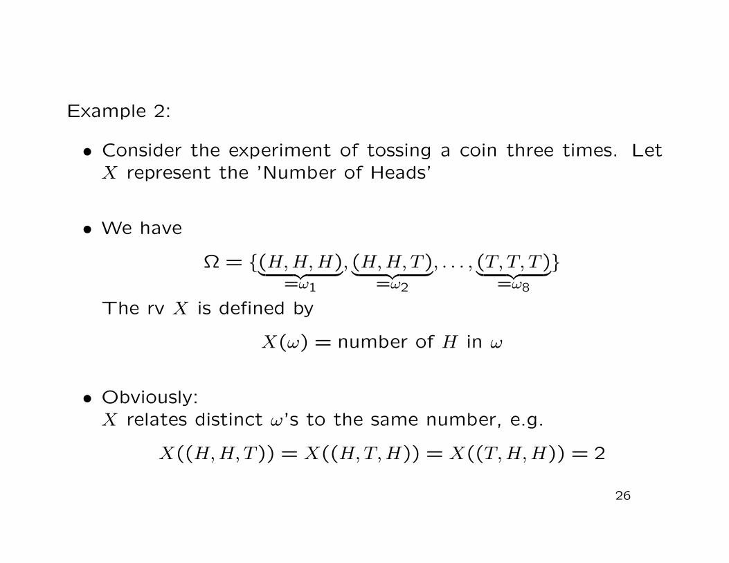
Example 2:

• Consider the experiment of tossing a coin three times. LetX represent the ’Number of Heads’

• We have

Ω = (H, H, H)︸ ︷︷ ︸

=ω1

, (H, H, T )︸ ︷︷ ︸

=ω2

, . . . , (T, T, T )︸ ︷︷ ︸

=ω8

The rv X is defined by

X(ω) = number of H in ω

• Obviously:X relates distinct ω’s to the same number, e.g.

X((H, H, T )) = X((H, T, H)) = X((T, H, H)) = 2

26

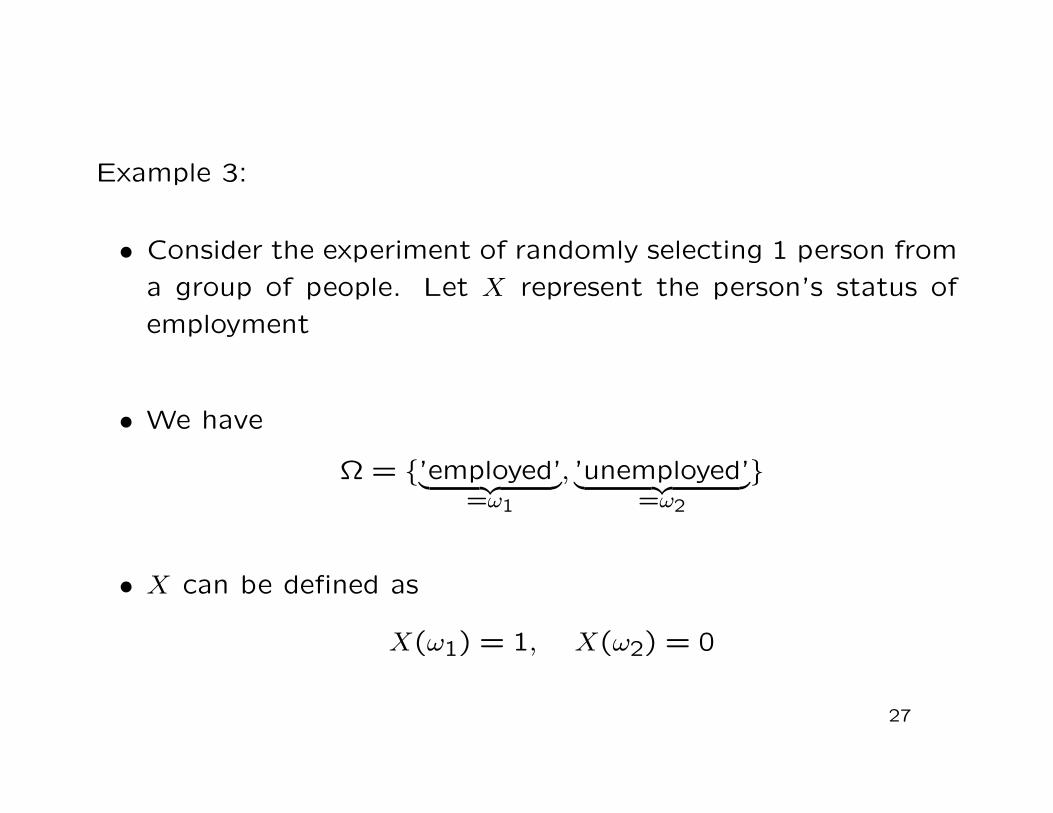
Example 3:

• Consider the experiment of randomly selecting 1 person froma group of people. Let X represent the person’s status ofemployment

• We have

Ω = ’employed’︸ ︷︷ ︸

=ω1

, ’unemployed’︸ ︷︷ ︸

=ω2

• X can be defined as

X(ω1) = 1, X(ω2) = 0

27

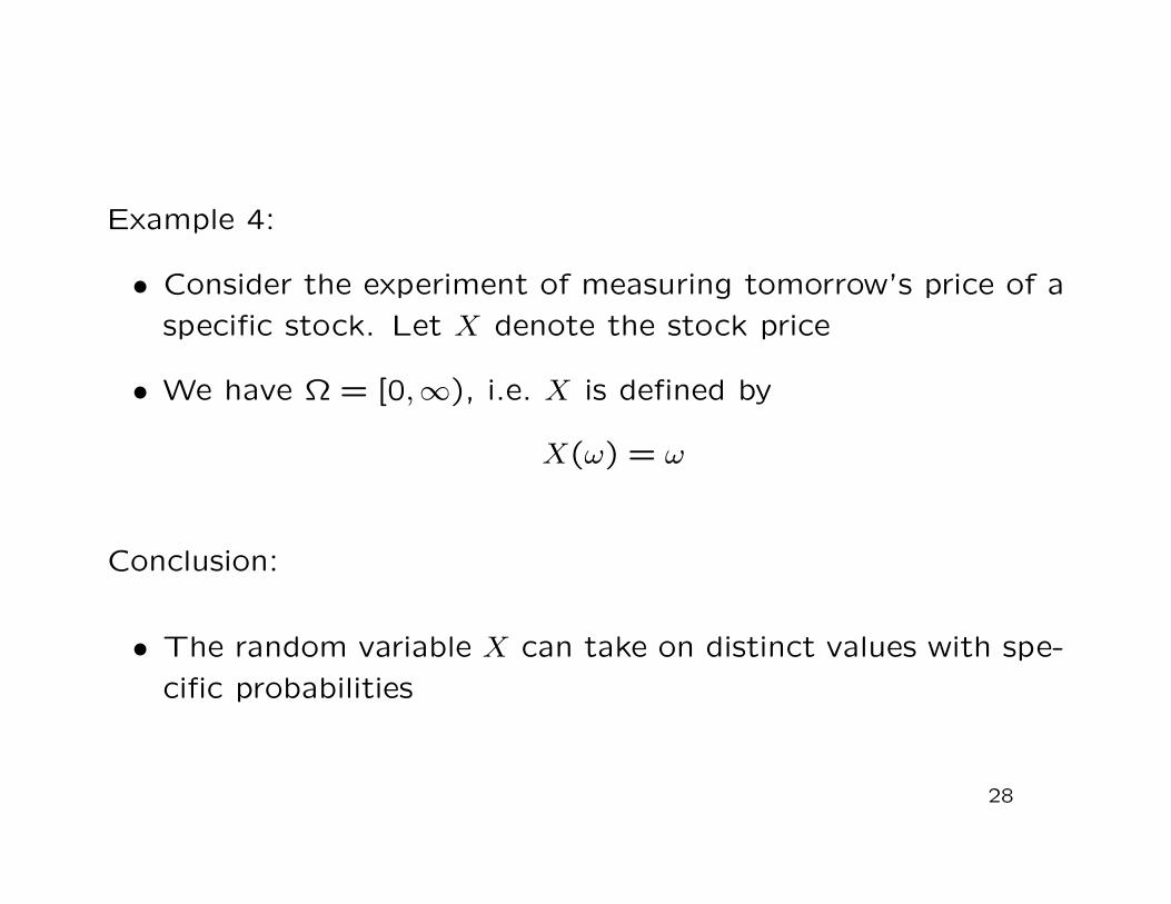
Example 4:

• Consider the experiment of measuring tomorrow’s price of aspecific stock. Let X denote the stock price

• We have Ω = [0,∞), i.e. X is defined by

X(ω) = ω

Conclusion:

• The random variable X can take on distinct values with spe-cific probabilities

28

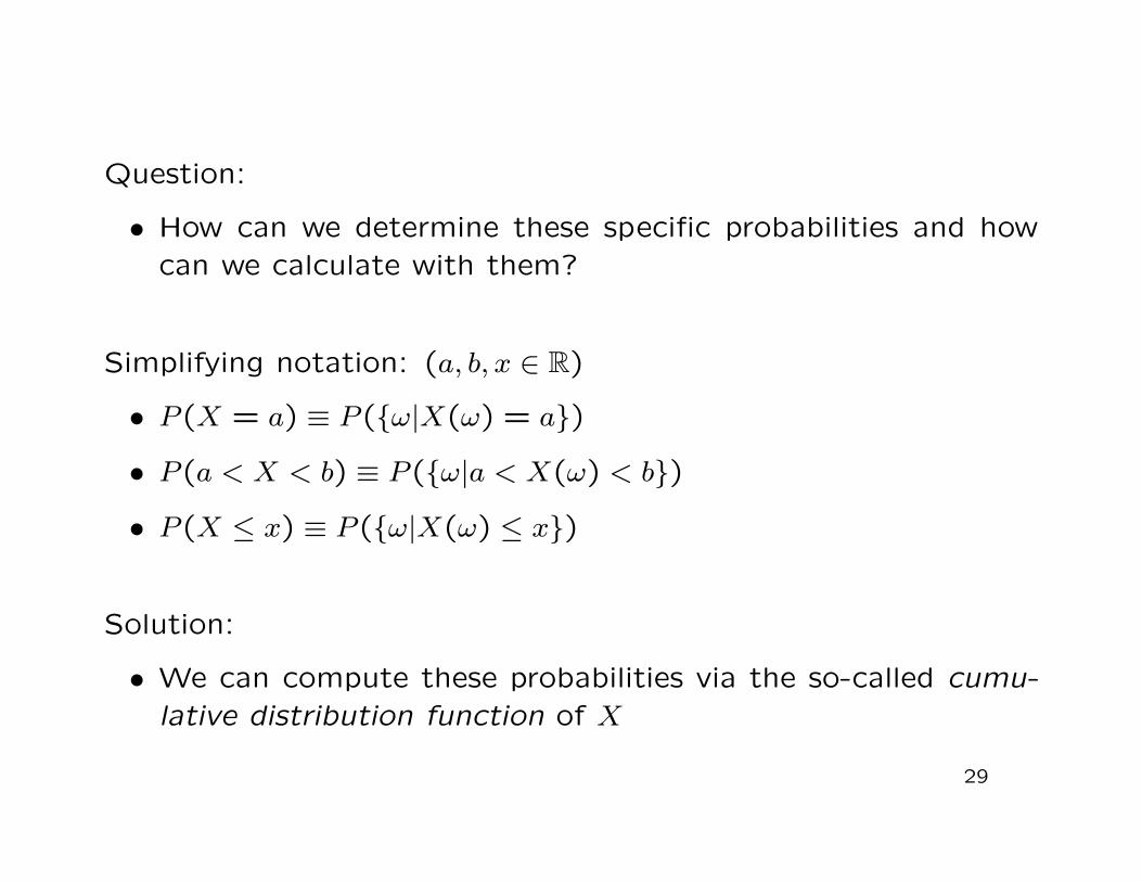
Question:

• How can we determine these specific probabilities and howcan we calculate with them?

Simplifying notation: (a, b, x ∈ R)

• P (X = a) ≡ P (ω|X(ω) = a)

• P (a < X < b) ≡ P (ω|a < X(ω) < b)

• P (X ≤ x) ≡ P (ω|X(ω) ≤ x)

Solution:

• We can compute these probabilities via the so-called cumu-lative distribution function of X

29

Intuitively:

• The cumulative distribution function of the random variableX characterizes the probabilities according to which the pos-sible values x are distributed along the real line(the so-called distribution of X)

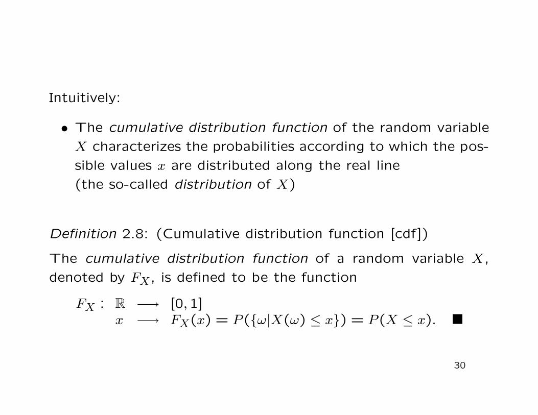
Definition 2.8: (Cumulative distribution function [cdf])

The cumulative distribution function of a random variable X,denoted by FX, is defined to be the function

FX : R −→ [0,1]x −→ FX(x) = P (ω|X(ω) ≤ x) = P (X ≤ x).

30

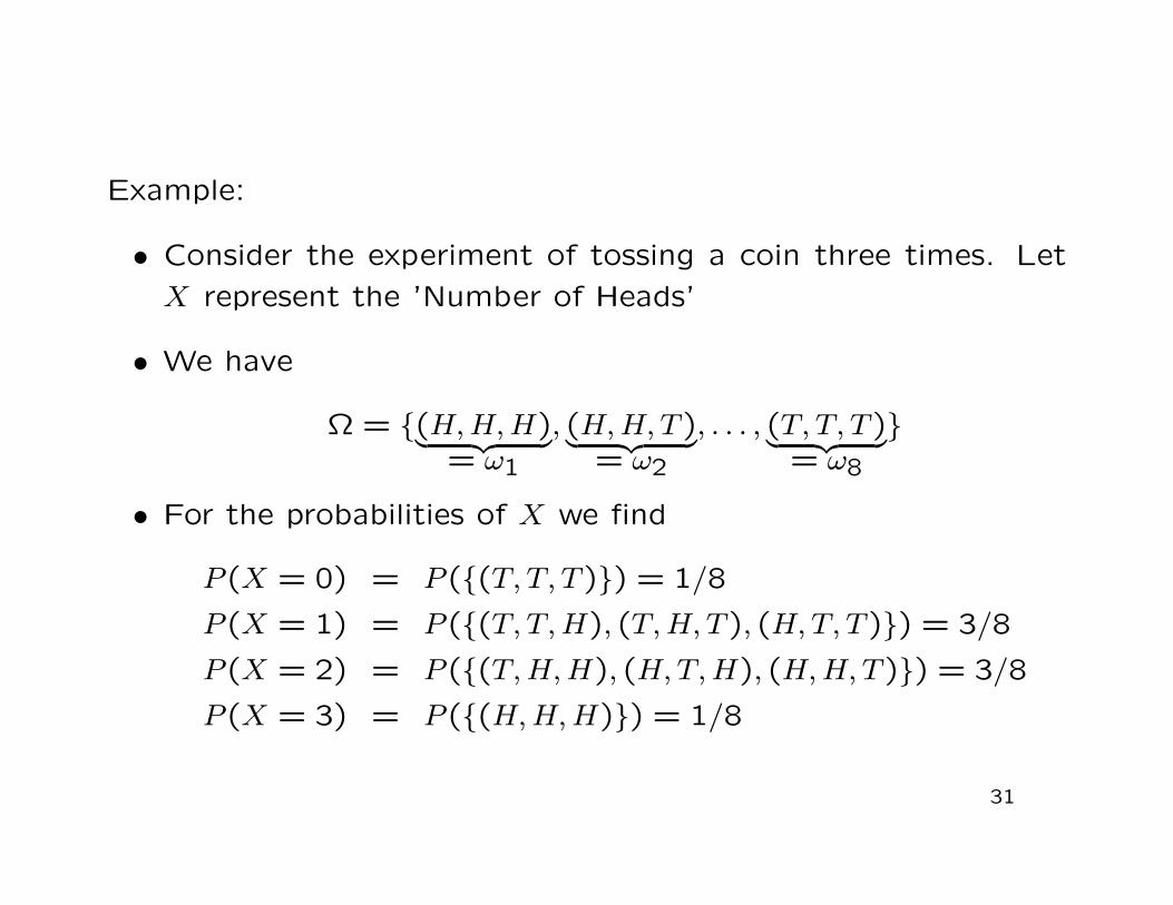
Example:

• Consider the experiment of tossing a coin three times. LetX represent the ’Number of Heads’

• We have

Ω = (H, H, H)︸ ︷︷ ︸

= ω1

, (H, H, T )︸ ︷︷ ︸

= ω2

, . . . , (T, T, T )︸ ︷︷ ︸

= ω8

• For the probabilities of X we find

P (X = 0) = P ((T, T, T )) = 1/8

P (X = 1) = P ((T, T, H), (T, H, T ), (H, T, T )) = 3/8

P (X = 2) = P ((T, H, H), (H, T, H), (H, H, T )) = 3/8

P (X = 3) = P ((H, H, H)) = 1/8

31

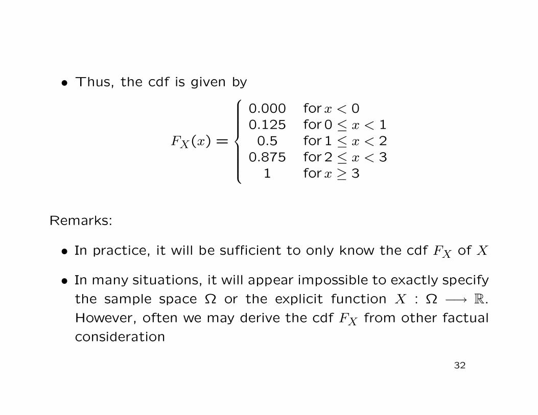
• Thus, the cdf is given by

FX(x) =

0.000 forx < 00.125 for 0 ≤ x < 10.5 for 1 ≤ x < 2

0.875 for 2 ≤ x < 31 forx ≥ 3

Remarks:

• In practice, it will be sufficient to only know the cdf FX of X

• In many situations, it will appear impossible to exactly specifythe sample space Ω or the explicit function X : Ω −→ R.However, often we may derive the cdf FX from other factualconsideration

32

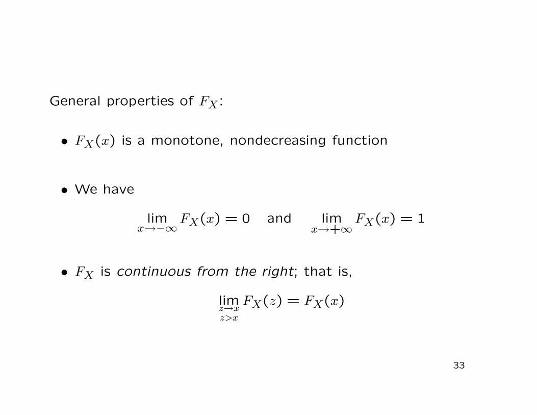
General properties of FX:

• FX(x) is a monotone, nondecreasing function

• We have

limx→−∞

FX(x) = 0 and limx→+∞

FX(x) = 1

• FX is continuous from the right; that is,

limz→xz>x

FX(z) = FX(x)

33

Summary:

• Via the cdf FX(x) we can answer the following question:

’What is the probability that the random variable X takeson a value that does not exceed x?’

Now:

• Consider the question:

’What is the value which X does not exceed with aprespecified probability p ∈ (0,1)?’

−→ quantile function of X

34

Definition 2.9: (Quantile function)

Consider the rv X with cdf FX. For every p ∈ (0,1) the quantilefunction of X, denoted by QX(p), is defined as

QX : (0,1) −→ Rp −→ QX(p) = minx|FX(x) ≥ p.

The value of the quantile function xp = QX(p) is called the pthquantile of X.

Remarks:

• The pth quantile xp of X is defined as the smallest numberx satisfying FX(x) ≥ p

• In other words: The pth quantile xp is the smallest value thatX does not exceed with probability p

35

Special quantiles:

• Median: p = 0.5

• Quartiles: p = 0.25,0.5,0.75

• Quintiles: p = 0.2,0.4,0.6,0.8

• Deciles: p = 0.1,0.2, . . . ,0.9

Now:

• Consideration of two distinct classes of random variables(discrete vs. continuous rv’s)

36

Reason:

• Each class requires a specific mathematical treatment

Mathematical tools for analyzing discrete rv’s:

• Finite and infinite sums

Mathematical tools for analyzing continuous rv’s:

• Differential- and integral calculus

Remarks:

• Some rv’s are partly discrete and partly continuous

• Such rv’s are not treated in this course

37

Definition 2.10: (Discrete random variable)

A random variable X will be defined to be discrete if it can takeon either

(a) only a finite number of values x1, x2, . . . , xJ or

(b) an infinite, but countable number of values x1, x2, . . .

each with strictly positive probability; that is, if for all j =1, . . . , J, . . . we have

P (X = xj) > 0 andJ,...∑

j=1P (X = xj) = 1.

38

Examples of discrete variables:

• Countable variables (’X = Number of . . .’)

• Encoded qualitative variables

Further definitions:

Definition 2.11: (Support of a discrete random variable)

The support of a discrete rv X, denoted by supp(X), is definedto be the totality of all values that X can take on with a strictlypositive probability:

supp(X) = x1, . . . , xJ or supp(X) = x1, x2, . . ..

39

Definition 2.12: (Discrete density function)

For a discrete random variable X the function

fX(x) = P (X = x)

is defined to be the discrete density function of X.

Remarks:

• The discrete density function fX(·) takes on strictly positivevalues only for elements of the support of X. For realizationsof X that do not belong to the support of X, i.e. for x /∈supp(X), we have fX(x) = 0:

fX(x) =

P (X = xj) > 0 forx = xj ∈ supp(X)0 forx /∈ supp(X)

40

• The discrete density function fX(·) has the following proper-ties:

fX(x) ≥ 0 for all x

∑

xj∈supp(X)

fX(xj) = 1

• For any arbitrary set A ⊂ R the probability of the eventω|X(ω) ∈ A = X ∈ A is given by

P (X ∈ A) =∑

xj∈AfX(xj)

41

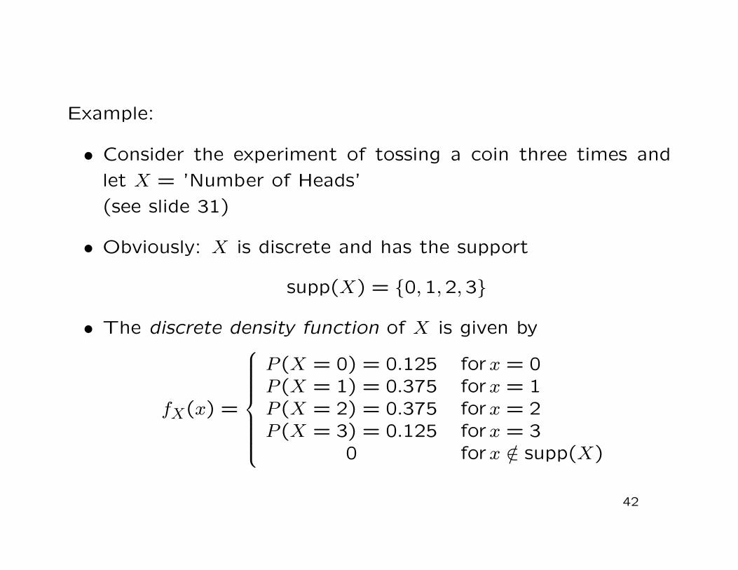
Example:

• Consider the experiment of tossing a coin three times andlet X = ’Number of Heads’(see slide 31)

• Obviously: X is discrete and has the support

supp(X) = 0,1,2,3

• The discrete density function of X is given by

fX(x) =

P (X = 0) = 0.125 forx = 0P (X = 1) = 0.375 forx = 1P (X = 2) = 0.375 forx = 2P (X = 3) = 0.125 forx = 3

0 forx /∈ supp(X)

42

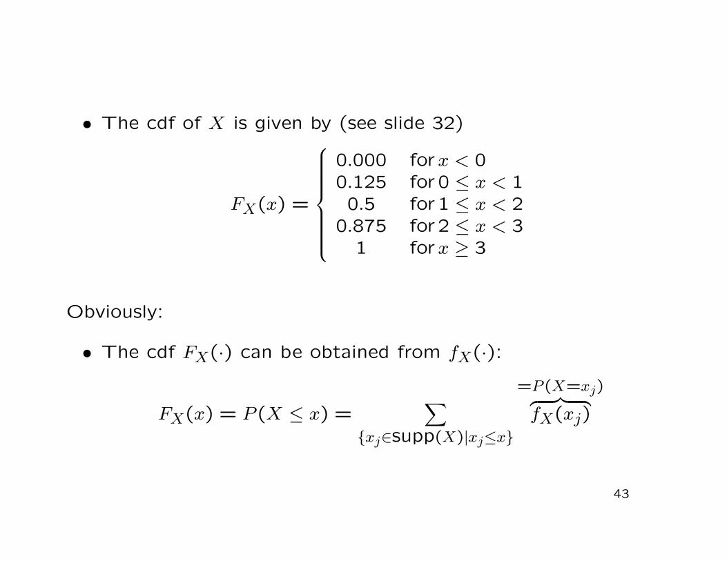
• The cdf of X is given by (see slide 32)

FX(x) =

0.000 forx < 00.125 for 0 ≤ x < 10.5 for 1 ≤ x < 2

0.875 for 2 ≤ x < 31 forx ≥ 3

Obviously:

• The cdf FX(·) can be obtained from fX(·):

FX(x) = P (X ≤ x) =∑

xj∈supp(X)|xj≤x

=P (X=xj)︷ ︸︸ ︷

fX(xj)

43

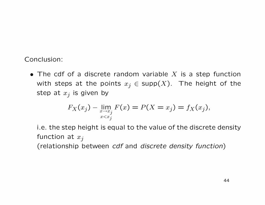
Conclusion:

• The cdf of a discrete random variable X is a step functionwith steps at the points xj ∈ supp(X). The height of thestep at xj is given by

FX(xj)− limx→xjx<xj

F (x) = P (X = xj) = fX(xj),

i.e. the step height is equal to the value of the discrete densityfunction at xj(relationship between cdf and discrete density function)

44

Now:

• Definition of continuous random variables

Intuitively:

• In contrast to discrete random variables, continuous randomvariables can take on an uncountable number of values(e.g. every real number on a given interval)

In fact:

• Definition of a continuous random variable is quite technical

45

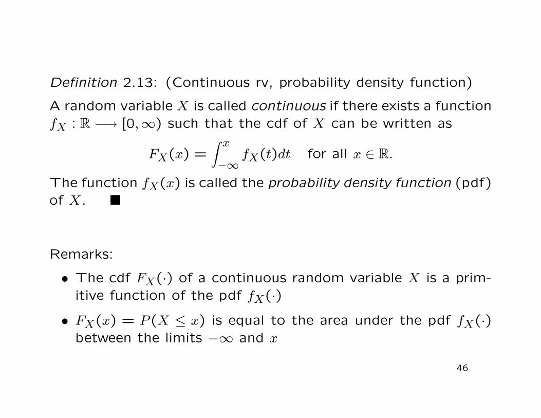
Definition 2.13: (Continuous rv, probability density function)

A random variable X is called continuous if there exists a functionfX : R −→ [0,∞) such that the cdf of X can be written as

FX(x) =∫ x

−∞fX(t)dt for all x ∈ R.

The function fX(x) is called the probability density function (pdf)of X.

Remarks:

• The cdf FX(·) of a continuous random variable X is a prim-itive function of the pdf fX(·)

• FX(x) = P (X ≤ x) is equal to the area under the pdf fX(·)between the limits −∞ and x

46

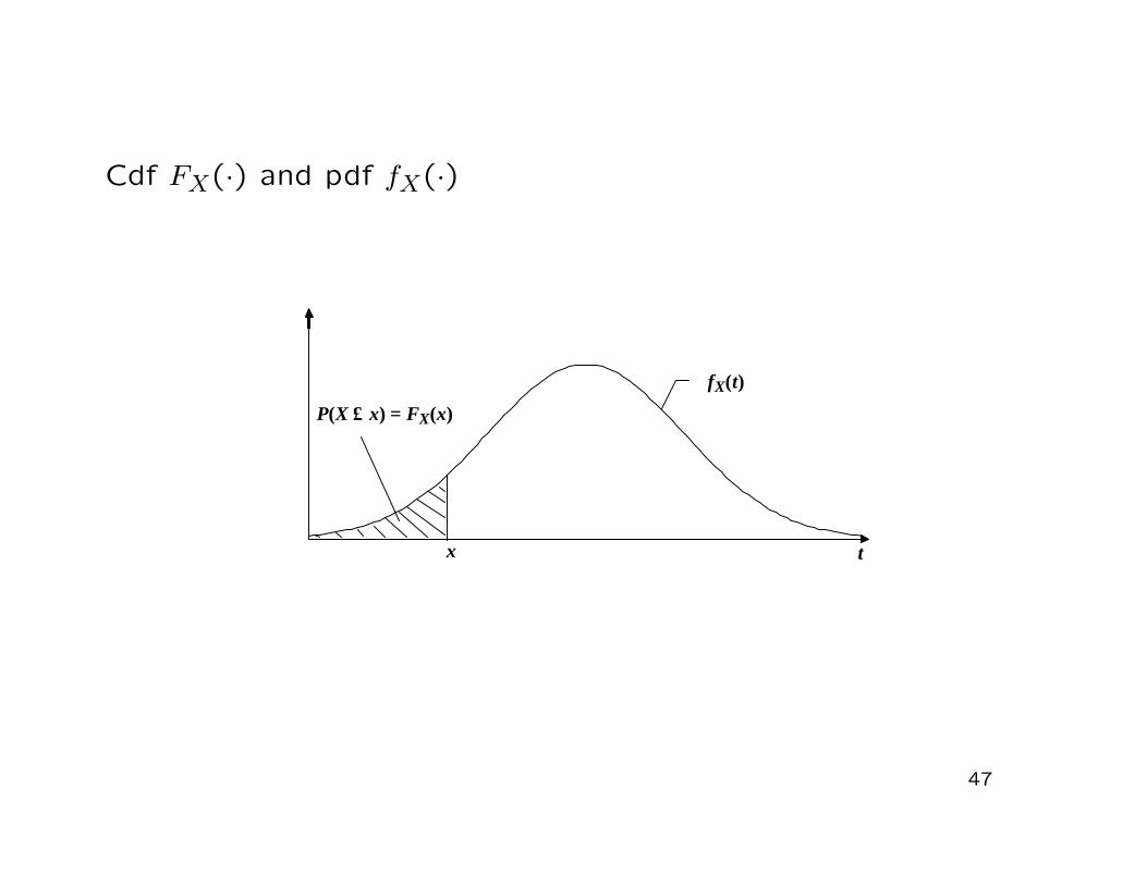
Cdf FX(·) and pdf fX(·)

47

x

fX(t)

P(X ≤ x) = FX(x)

t

Properties of the pdf fX(·):

1. A pdf fX(·) cannot take on negative value, i.e.

fX(x) ≥ 0 for all x ∈ R

2. The area under a pdf is equal to one, i.e.∫ +∞

−∞fX(x)dx = 1

3. If the cdf FX(x) is differentiable we have

fX(x) = F ′X(x) ≡ dFX(x)/dx

48

Example: (Uniform distribution over [0,10])

• Consider the random variable X with pdf

fX(x) =

0 , for x /∈ [0,10]0.1 , for x ∈ [0,10]

• Derivation of the cdf FX:For x < 0 we have

FX(x) =∫ x

−∞fX(t) dt =

∫ x

−∞0 dt = 0

49

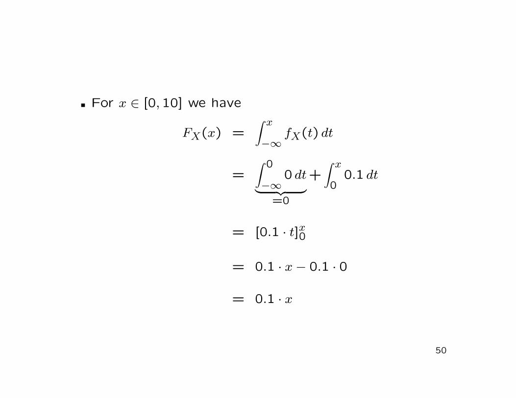
For x ∈ [0,10] we have

FX(x) =∫ x

−∞fX(t) dt

=∫ 0

−∞0 dt

︸ ︷︷ ︸

=0

+∫ x

00.1 dt

= [0.1 · t]x0

= 0.1 · x− 0.1 · 0

= 0.1 · x

50

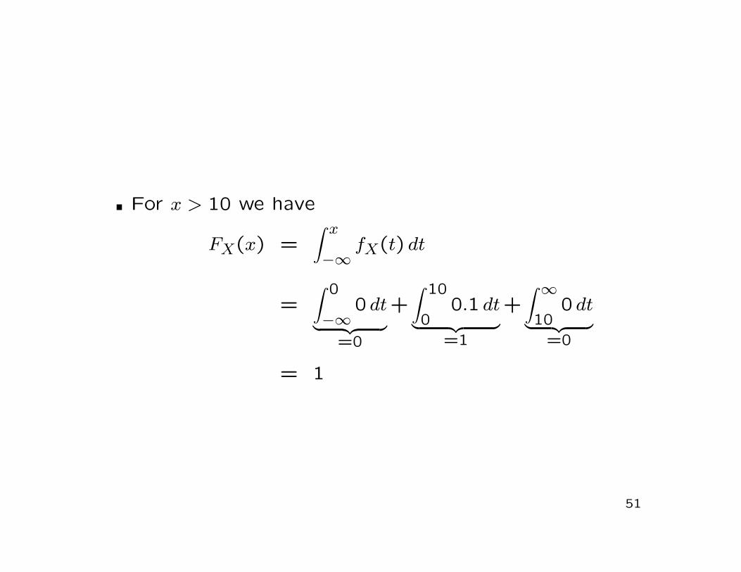
For x > 10 we have

FX(x) =∫ x

−∞fX(t) dt

=∫ 0

−∞0 dt

︸ ︷︷ ︸

=0

+∫ 10

00.1 dt

︸ ︷︷ ︸

=1

+∫ ∞

100 dt

︸ ︷︷ ︸

=0

= 1

51

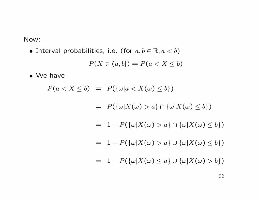
Now:

• Interval probabilities, i.e. (for a, b ∈ R, a < b)

P (X ∈ (a, b]) = P (a < X ≤ b)

• We have

P (a < X ≤ b) = P (ω|a < X(ω) ≤ b)

= P (ω|X(ω) > a ∩ ω|X(ω) ≤ b)

= 1− P (ω|X(ω) > a ∩ ω|X(ω) ≤ b)

= 1− P (ω|X(ω) > a ∪ ω|X(ω) ≤ b)

= 1− P (ω|X(ω) ≤ a ∪ ω|X(ω) > b)

52

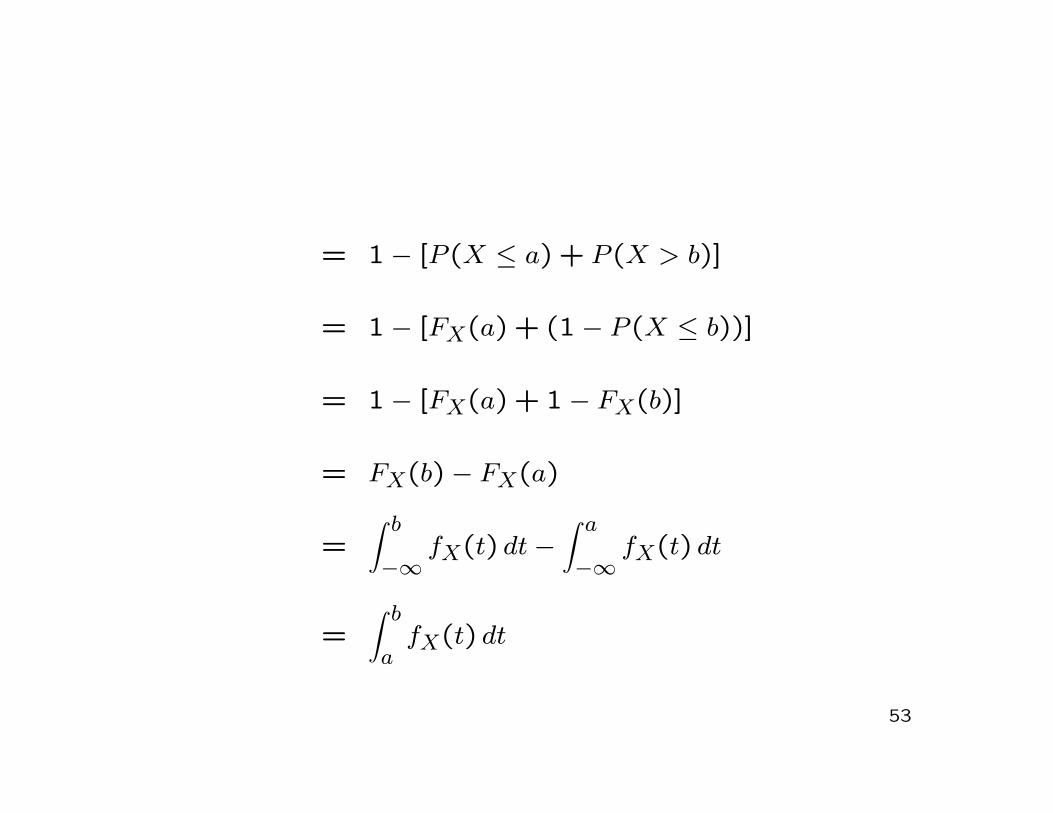
= 1− [P (X ≤ a) + P (X > b)]

= 1− [FX(a) + (1− P (X ≤ b))]

= 1− [FX(a) + 1− FX(b)]

= FX(b)− FX(a)

=∫ b

−∞fX(t) dt−

∫ a

−∞fX(t) dt

=∫ b

afX(t) dt

53

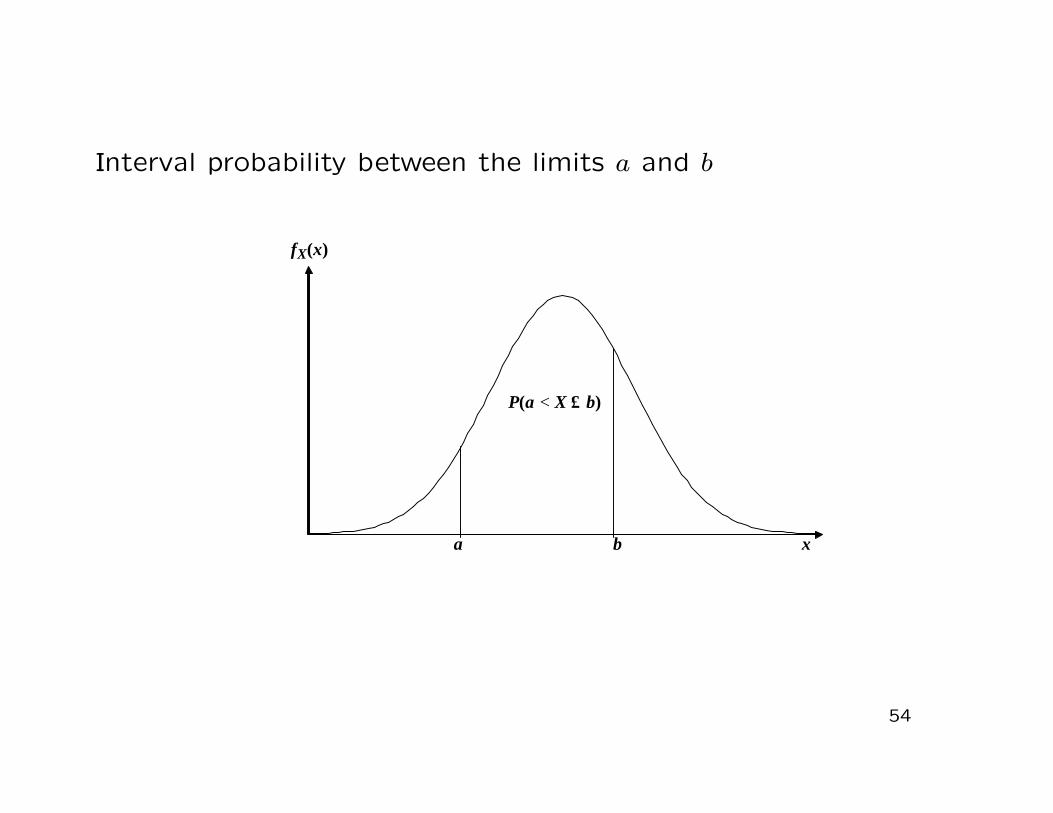
Interval probability between the limits a and b

54

a x b

fX(x)

P(a < X ≤ b)

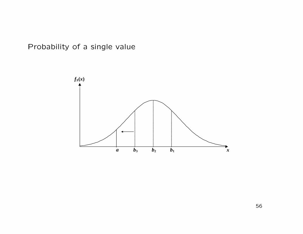
Important result for a continuous rv X:

P (X = a) = 0 for all a ∈ R

Proof:

P (X = a) = limb→a

P (a < X ≤ b) = limb→a

∫ b

afX(x) dx

=∫ a

afX(x)dx = 0

Conclusion:

• The probability that a continuous random variable X takeson a single explicit value is always zero

55

Probability of a single value

56

a b1b2b3

fX(x)

x

Notice:

• This does not imply that the event X = a cannot occur

Consequence:

• Since for continuous random variables we always have P (X =a) = 0 for all a ∈ R, it follows that

P (a < X < b) = P (a ≤ X < b) = P (a ≤ X ≤ b)

= P (a < X ≤ b) = FX(b)− FX(a)

(when computing interval probabilities for continuous rv’s, itdoes not matter if the interval is open or closed)

57

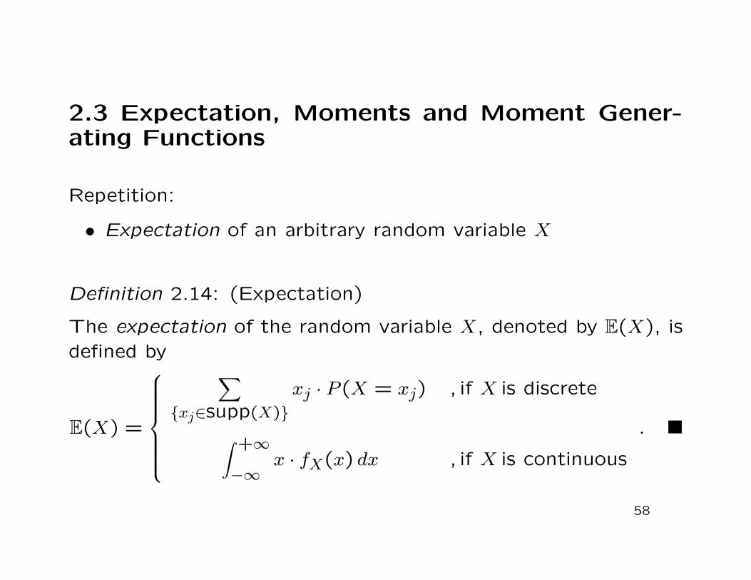
2.3 Expectation, Moments and Moment Gener-ating Functions

Repetition:

• Expectation of an arbitrary random variable X

Definition 2.14: (Expectation)

The expectation of the random variable X, denoted by E(X), isdefined by

E(X) =

∑

xj∈supp(X)xj · P (X = xj) , if X is discrete

∫ +∞

−∞x · fX(x) dx , if X is continuous

.

58

Remarks:

• The expectation of the random variable X is approximatelyequal to the sum of all realizations each weighted by theprobability of its occurrence

• Instead of E(X) we often write µX

• There exist random variables that do not have an expectation(see class)

59

Example 1: (Discrete random variable)

• Consider the experiment of tossing two dice. Let X repre-sent the absolute difference of the two dice. What is theexpectation of X?

• The support of X is given by

supp(X) = 0,1,2,3,4,5

60

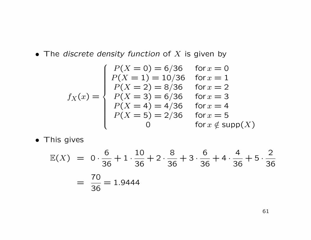
• The discrete density function of X is given by

fX(x) =

P (X = 0) = 6/36 forx = 0P (X = 1) = 10/36 forx = 1P (X = 2) = 8/36 forx = 2P (X = 3) = 6/36 forx = 3P (X = 4) = 4/36 forx = 4P (X = 5) = 2/36 forx = 5

0 forx /∈ supp(X)

• This gives

E(X) = 0 ·636

+ 1 ·1036

+ 2 ·836

+ 3 ·636

+ 4 ·436

+ 5 ·236

=7036

= 1.9444

61

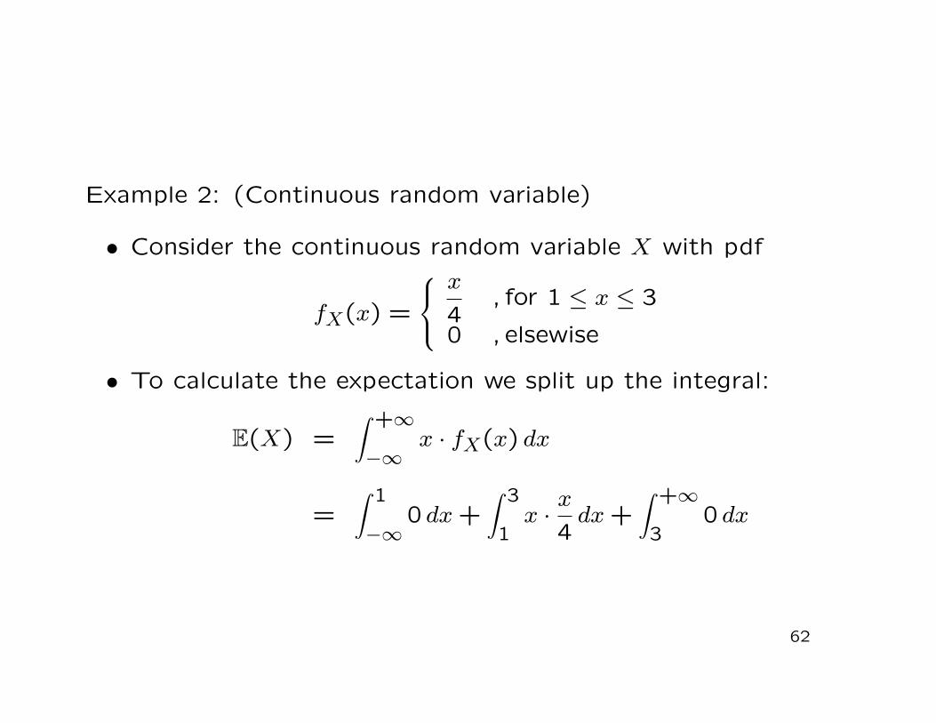
Example 2: (Continuous random variable)

• Consider the continuous random variable X with pdf

fX(x) =

x4

, for 1 ≤ x ≤ 3

0 , elsewise

• To calculate the expectation we split up the integral:

E(X) =∫ +∞

−∞x · fX(x) dx

=∫ 1

−∞0 dx +

∫ 3

1x ·

x4

dx +∫ +∞

30 dx

62

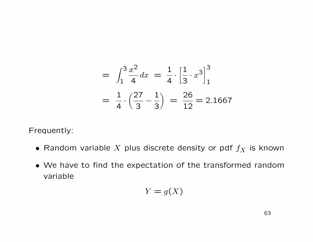
=∫ 3

1

x2

4dx =

14·[13· x3

]3

1

=14·(27

3−

13

)

=2612

= 2.1667

Frequently:

• Random variable X plus discrete density or pdf fX is known

• We have to find the expectation of the transformed randomvariable

Y = g(X)

63

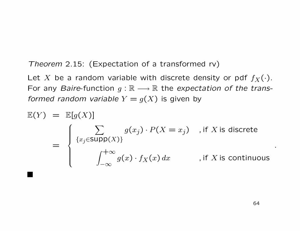
Theorem 2.15: (Expectation of a transformed rv)

Let X be a random variable with discrete density or pdf fX(·).For any Baire-function g : R −→ R the expectation of the trans-formed random variable Y = g(X) is given by

E(Y ) = E[g(X)]

=

∑

xj∈supp(X)g(xj) · P (X = xj) , if X is discrete

∫ +∞

−∞g(x) · fX(x) dx , if X is continuous

.

64

Remarks:

• All functions considered in this course are Baire-functions

• For the special case g(x) = x (the identity function) Theorem2.15 coincides with Definition 2.14

Next:

• Some important rules for calculating expected values

65

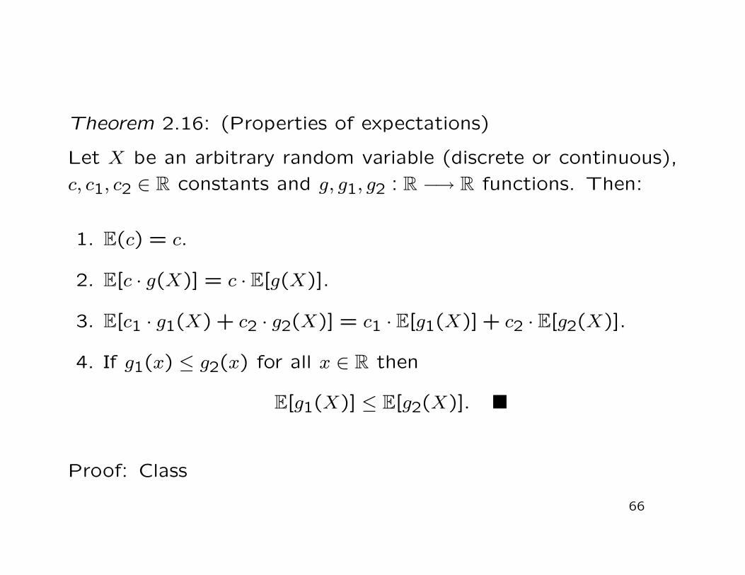
Theorem 2.16: (Properties of expectations)

Let X be an arbitrary random variable (discrete or continuous),c, c1, c2 ∈ R constants and g, g1, g2 : R −→ R functions. Then:

1. E(c) = c.

2. E[c · g(X)] = c · E[g(X)].

3. E[c1 · g1(X) + c2 · g2(X)] = c1 · E[g1(X)] + c2 · E[g2(X)].

4. If g1(x) ≤ g2(x) for all x ∈ R then

E[g1(X)] ≤ E[g2(X)].

Proof: Class

66

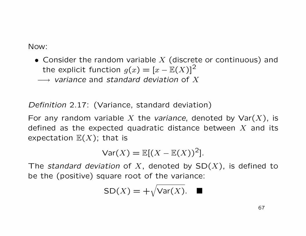
Now:

• Consider the random variable X (discrete or continuous) andthe explicit function g(x) = [x− E(X)]2

−→ variance and standard deviation of X

Definition 2.17: (Variance, standard deviation)

For any random variable X the variance, denoted by Var(X), isdefined as the expected quadratic distance between X and itsexpectation E(X); that is

Var(X) = E[(X − E(X))2].

The standard deviation of X, denoted by SD(X), is defined tobe the (positive) square root of the variance:

SD(X) = +√

Var(X).

67

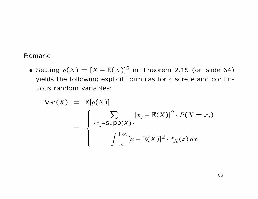
Remark:

• Setting g(X) = [X − E(X)]2 in Theorem 2.15 (on slide 64)yields the following explicit formulas for discrete and contin-uous random variables:

Var(X) = E[g(X)]

=

∑

xj∈supp(X)[xj − E(X)]2 · P (X = xj)

∫ +∞

−∞[x− E(X)]2 · fX(x) dx

68

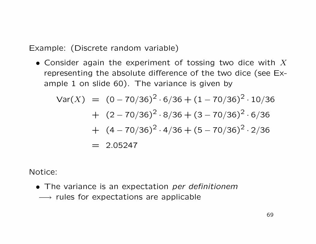
Example: (Discrete random variable)

• Consider again the experiment of tossing two dice with Xrepresenting the absolute difference of the two dice (see Ex-ample 1 on slide 60). The variance is given by

Var(X) = (0− 70/36)2 · 6/36 + (1− 70/36)2 · 10/36

+ (2− 70/36)2 · 8/36 + (3− 70/36)2 · 6/36

+ (4− 70/36)2 · 4/36 + (5− 70/36)2 · 2/36

= 2.05247

Notice:

• The variance is an expectation per definitionem−→ rules for expectations are applicable

69

Theorem 2.18: (Rules for variances)

Let X be an arbitrary random variable (discrete or continuous)and a, b ∈ R real constants; then

1. Var(X) = E(X2)− [E(X)]2.

2. Var(a + b ·X) = b2 ·Var(X).

Proof: Class

Next:

• Two important inequalities dealing with expectations andtransformed random variables

70

Theorem 2.19: (Chebyshev inequality)

Let X be an arbitrary random variable and g : R −→ R+ a non-negative function. Then, for every k > 0 we have

P [g(X) ≥ k] ≤E [g(X)]

k.

Special case:

• Consider

g(x) = [x− E(X)]2 and k = r2 ·Var(X) (r > 0)

• Theorem 2.19 implies

P

[X − E(X)]2 ≥ r2 ·Var(X)

≤Var(X)

r2 ·Var(X)=

1r2

71

• Now:

P

[X − E(X)]2 ≥ r2 ·Var(X)

= P |X − E(X)| ≥ r · SD(X)

= 1− P |X − E(X)| < r · SD(X)

• It follows that

P |X − E(X)| < r · SD(X) ≥ 1−1r2

(specific Chebyshev inequality)

72

Remarks:

• The specific Chebyshev inequality provides a minimal proba-bility of the event that any arbitrary random variable X takeson a value from the following interval:

[E(X)− r · SD(X),E(X) + r · SD(X)]

• For example, for r = 3 we have

P |X − E(X)| < 3 · SD(X) ≥ 1−132 =

89

which is equivalent to

P E(X)− 3 · SD(X) < X < E(X) + 3 · SD(X) ≥ 0.8889

or

P X ∈ (E(X)− 3 · SD(X),E(X) + 3 · SD(X)) ≥ 0.8889

73

Theorem 2.20: (Jensen inequality)

Let X be a random variable with mean E(X) and let g : R −→ Rbe a convex function, i.e. for all x we have g′′(x) ≥ 0; then

E [g(X)] ≥ g(E[X]).

Remarks:

• If the function g is concave (i.e. if g′′(x) ≤ 0 for all x) thenJensen’s inequality states that E [g(X)] ≤ g(E[X])

• Notice that in general we have

E [g(X)] 6= g(E[X])

74

Example:

• Consider the random variable X and the function g(x) = x2

• We have g′′(x) = 2 ≥ 0 for all x, i.e. g is convex

• It follows from Jensen’s inequality that

E [g(X)]︸ ︷︷ ︸

=E(X2)

≥ g(E[X])︸ ︷︷ ︸

=[E(X)]2

i.e.

E(X2)− [E(X)]2 ≥ 0

• This implies

Var(X) = E(X2)− [E(X)]2 ≥ 0

(the variance of an arbitrary rv cannot be negative)

75

Now:

• Consider the random variable X with expectation E(X) = µX,the integer number n ∈ N and the functions

g1(x) = xn

g2(x) = [x− µX]n

Definition 2.21: (Moments, central moments)

(a) The n-th moment of X, denoted by µ′n, is defined as

µ′n ≡ E[g1(X)] = E(Xn).

(b) The n-th central moment of X about µX, denoted by µn, isdefined as

µn ≡ E[g2(X)] = E[(X − µX)n].

76

Relations:

• µ′1 = E(X) = µX(the 1st moment coincides with E(X))

• µ1 = E[X − µX] = E(X)− µX = 0(the 1st central moment is always equal to 0)

• µ2 = E[(X − µX)2] = Var(X)(the 2nd central moment coincides with Var(X))

77

Remarks:

• The first four moments of a random variable X are importantmeasures of the probability distribution(expectation, variance, skewness, kurtosis)

• The moments of a random variable X play an important rolein theoretical and applied statistics

• In some cases, when all moments are known, the cdf of arandom variable X can be determined

78

Question:

• Can we find a function that gives us a representation of allmoments of a random variable X?

Definition 2.22: (Moment generating function)

Let X be a random variable with discrete density or pdf fX(·).The expected value of et·X is defined to be the moment gener-ating function of X if the expected value exists for every valueof t in some interval −h < t < h, h > 0. That is, the momentgenerating function of X, denoted by mX(t), is defined as

mX(t) = E[

et·X]

.

79

Remarks:

• The moment generating function mX(t) is a function in t

• There are rv’s X for which mX(t) does not exist

• If mX(t) exists it can be calculated as

mX(t) = E[

et·X]

=

∑

xj∈supp(X)et·xj · P (X = xj) , if X is discrete

∫ +∞

−∞et·x · fX(x) dx , if X is continuous

80

Question:

• Why is mX(t) called the moment generating function?

Answer:

• Consider the nth derivative of mX(t) with respect to t:

dn

dtnmX(t) =

∑

xj∈supp(X)(xj)

n · et·xj · P (X = xj) for discrete X

∫ +∞

−∞xn · et·x · fX(x) dx for continuous X

81

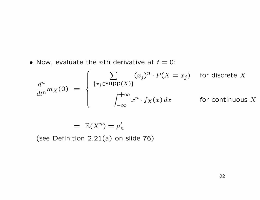
• Now, evaluate the nth derivative at t = 0:

dn

dtnmX(0) =

∑

xj∈supp(X)(xj)

n · P (X = xj) for discrete X

∫ +∞

−∞xn · fX(x) dx for continuous X

= E(Xn) = µ′n

(see Definition 2.21(a) on slide 76)

82

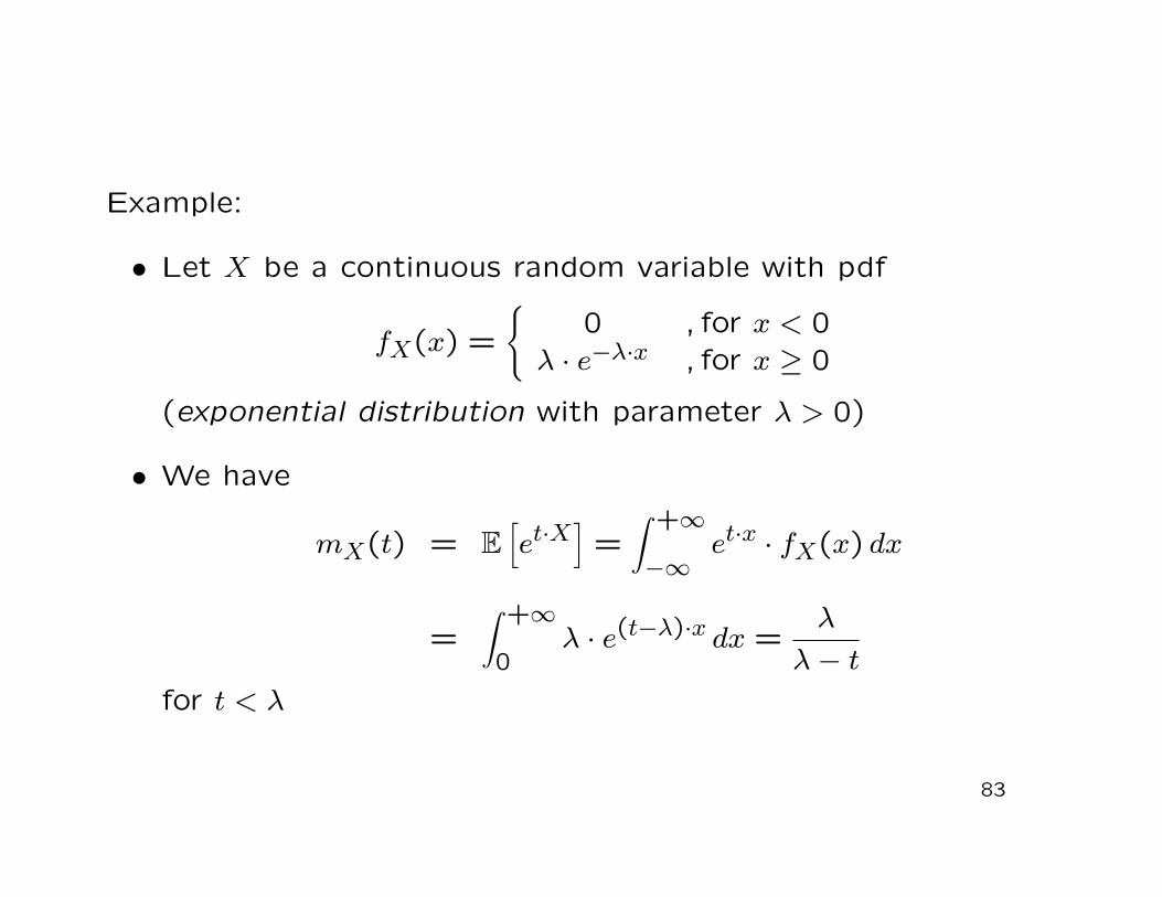
Example:

• Let X be a continuous random variable with pdf

fX(x) =

0 , for x < 0λ · e−λ·x , for x ≥ 0

(exponential distribution with parameter λ > 0)

• We have

mX(t) = E[

et·X]

=∫ +∞

−∞et·x · fX(x) dx

=∫ +∞

0λ · e(t−λ)·x dx =

λλ− t

for t < λ

83

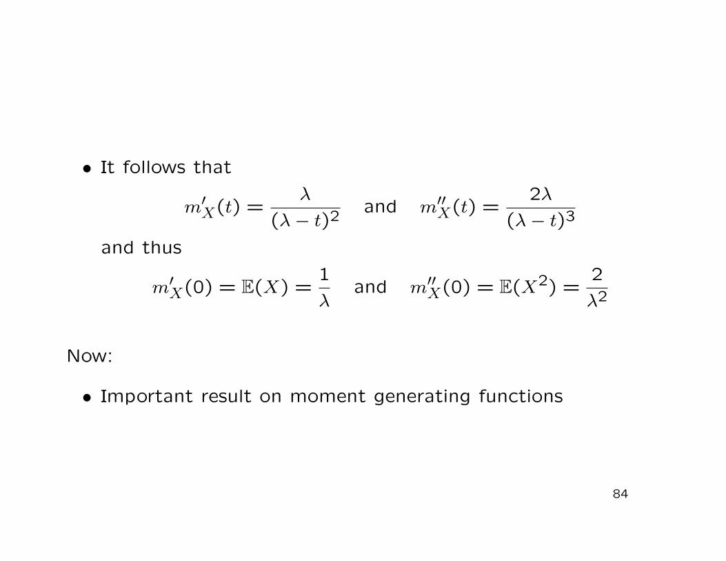
• It follows that

m′X(t) =

λ(λ− t)2

and m′′X(t) =

2λ(λ− t)3

and thus

m′X(0) = E(X) =

1λ

and m′′X(0) = E(X2) =

2λ2

Now:

• Important result on moment generating functions

84

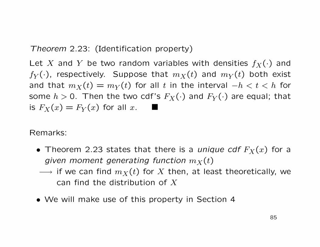
Theorem 2.23: (Identification property)

Let X and Y be two random variables with densities fX(·) andfY (·), respectively. Suppose that mX(t) and mY (t) both existand that mX(t) = mY (t) for all t in the interval −h < t < h forsome h > 0. Then the two cdf’s FX(·) and FY (·) are equal; thatis FX(x) = FY (x) for all x.

Remarks:

• Theorem 2.23 states that there is a unique cdf FX(x) for agiven moment generating function mX(t)−→ if we can find mX(t) for X then, at least theoretically, we

can find the distribution of X

• We will make use of this property in Section 4

85

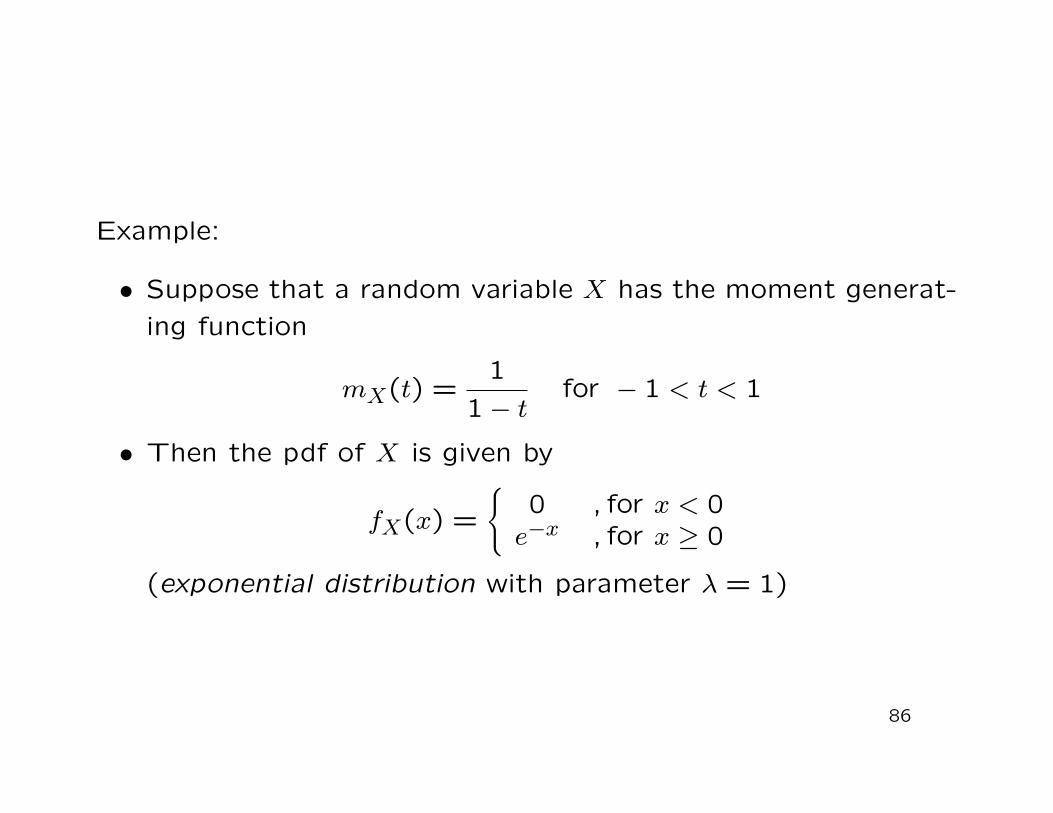
Example:

• Suppose that a random variable X has the moment generat-ing function

mX(t) =1

1− tfor − 1 < t < 1

• Then the pdf of X is given by

fX(x) =

0 , for x < 0e−x , for x ≥ 0

(exponential distribution with parameter λ = 1)

86

2.4 Special Parametric Families of Univariate Dis-tributions

Up to now:

• General mathematical properties of arbitrary distributions

• Discrimination: discrete vs continuous distributions

• Consideration of

the cdf FX(x)

the discrete density or the pdf fX(x)

expectations of the form E[g(X)]

the moment generating function mX(t)

87

Central result:

• The distribution of a random variable X is (essentially) de-termined by fX(x) or FX(x)

• FX(x) can be determined by fX(x)(cf. slide 46)

• fX(x) can be determined by FX(x)(cf. slide 48)

Question:

• How many different distributions are known to exist?

88

Answer:

• Infinitely many

But:

• In practice, there are some important parametric families ofdistributions that provide ’good’ models for representing real-world random phenomena

• These families of distributions are decribed in detail in alltextbooks on mathematical statistics(see e.g. Mosler & Schmid (2008), Mood et al. (1974))

89

• Important families of discrete distributions

Bernoulli distribution

Binomial distribution

Geometric distribution

Poisson distribution

• Important families of continuous distributions

Uniform or rectangular distribution

Exponential distribution

Normal distribution

90

Remark:

• The most important family of distributions at all is the nor-mal distribution

Definition 2.24: (Normal distribution)

A continuous random variable X is defined to be normally dis-tributed with parameters µ ∈ R and σ2 > 0, denoted by X ∼N(µ, σ2), if its pdf is given by

fX(x) =1√

2π · σ· e−

12

(

x−µσ

)2

, x ∈ R.

91

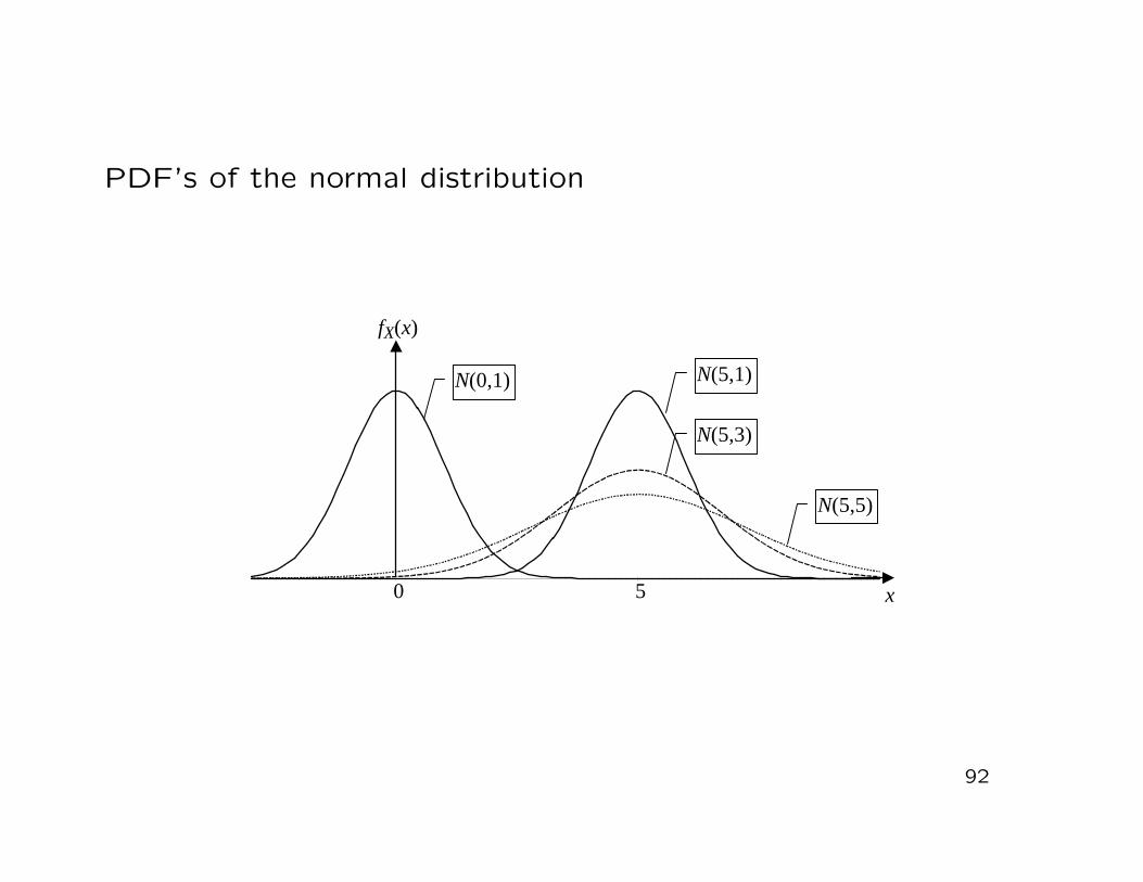
PDF’s of the normal distribution

92

0 5 x

fX(x)

N(0,1) N(5,1)

N(5,3)

N(5,5)

Remarks:

• The special normal distribution N(0,1) is called standard nor-mal distribution the pdf of which is denoted by ϕ(x)

• The properties as well as calculation rules for normally dis-tributed random variables are important pre-conditions forthis course(see Wilfling (2014), Section 3.4)

93

3. Joint and Conditional Distributions, StochasticIndependence

Aim of this section:

• Multidimensional random variables (random vectors)(joint and marginal distributions)

• Stochastic (in)dependence and conditional distribution

• Multivariate normal distribution(definition, properties)

Literature:

• Mood, Graybill, Boes (1974), Chapter IV, pp. 129-174

• Wilfling (2014), Chapter 4

94

3.1 Joint and Marginal Distribution

Now:

• Consider several random variables simultaneously

Applications:

• Several economic applications

• Statistical inference

95

Definition 3.1: (Random vector)

Let X1, · · · , Xn be a set of n random variables each representingthe same random experiment, i.e.

Xi : Ω −→ R for i = 1, . . . , n.

Then X = (X1, . . . , Xn)′ is called an n-dimensional random vari-able or an n-dimensional random vector.

Remark:

• In the literature random vectors are often denoted by

X = (X1, . . . , Xn) or more simply by X1, . . . , Xn

96

• For n = 2 it is common practice to write

X = (X, Y )′ or (X, Y ) or X, Y

• Realizations are denoted by small letters:

x = (x1, . . . , xn)′ ∈ Rn or x = (x, y)′ ∈ R2

Now:

• Characterization of the probability distribution of the randomvector X

97

Definition 3.2: (Joint cumulative distribution function)

Let X = (X1, . . . , Xn)′ be an n-dimensional random vector. Thefunction

FX1,...,Xn : Rn −→ [0,1]

defined by

FX1,...,Xn(x1, . . . , xn) = P (X1 ≤ x1, X2 ≤ x2, . . . , Xn ≤ xn)

is called the joint cumulative distribution function of X.

Remark:

• Definition 3.2 applies to discrete as well as to continuousrandom variables X1, . . . , Xn

98

Some properties of the bivariate cdf (n = 2):

• FX,Y (x, y) is monotone increasing in x and y

• limx→−∞

FX,Y (x, y) = 0

• limy→−∞

FX,Y (x, y) = 0

• limx→+∞y→+∞

FX,Y (x, y) = 1

Remark:

• Analogous properties hold for the n-dimensional cdfFX1,...,Xn(x1, . . . , xn)

99

Now:

• Joint discrete versus joint continuous random vectors

Definition 3.3: (Joint discrete random vector)

The random vector X = (X1, . . . , Xn)′ is defined to be a joint dis-crete random vector if it can assume only a finite (or a countableinfinite) number of realizations x = (x1, . . . , xn)′ such that

P (X1 = x1, X2 = x2, . . . , Xn = xn) > 0

and∑

P (X1 = x1, X2 = x2, . . . , Xn = xn) = 1,

where the summation is over all possible realizations of X.

100

Definition 3.4: (Joint continuous random vector)

The random vector X = (X1, . . . , Xn)′ is defined to be a jointcontinuous random vector if and only if there exists a nonnegativefunction fX1,...,Xn(x1, . . . , xn) such that

FX1,...,Xn(x1, . . . , xn) =∫ xn

−∞. . .

∫ x1

−∞fX1,...,Xn(u1, . . . , un) du1 . . . dun

for all (x1, . . . , xn). The function fX1,...,Xn is defined to be a jointprobability density function of X.

Example:

• Consider X = (X, Y )′ with joint pdf

fX,Y (x, y) =

x + y , for (x, y) ∈ [0,1]× [0,1]0 , elsewise

101

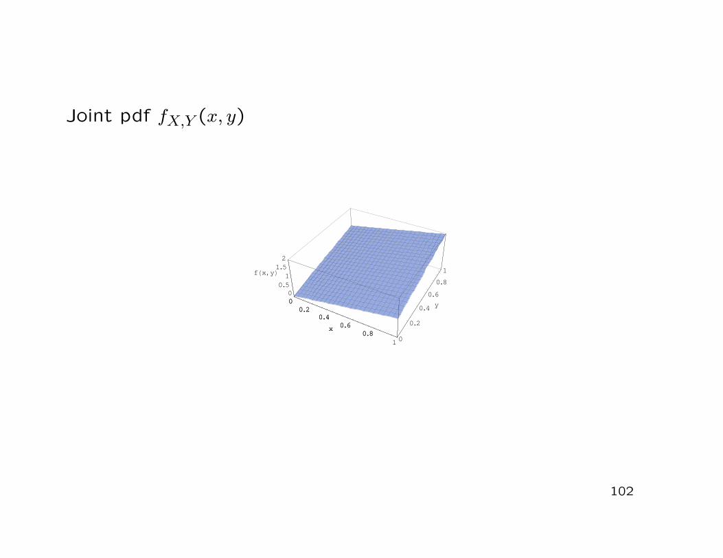
Joint pdf fX,Y (x, y)

102

00.2

0.40.6

0.81

x0

0.2

0.4

0.6

0.8

1

y

00.5

11.5

2

fHx,yL

00.2

0.40.6

0.8x

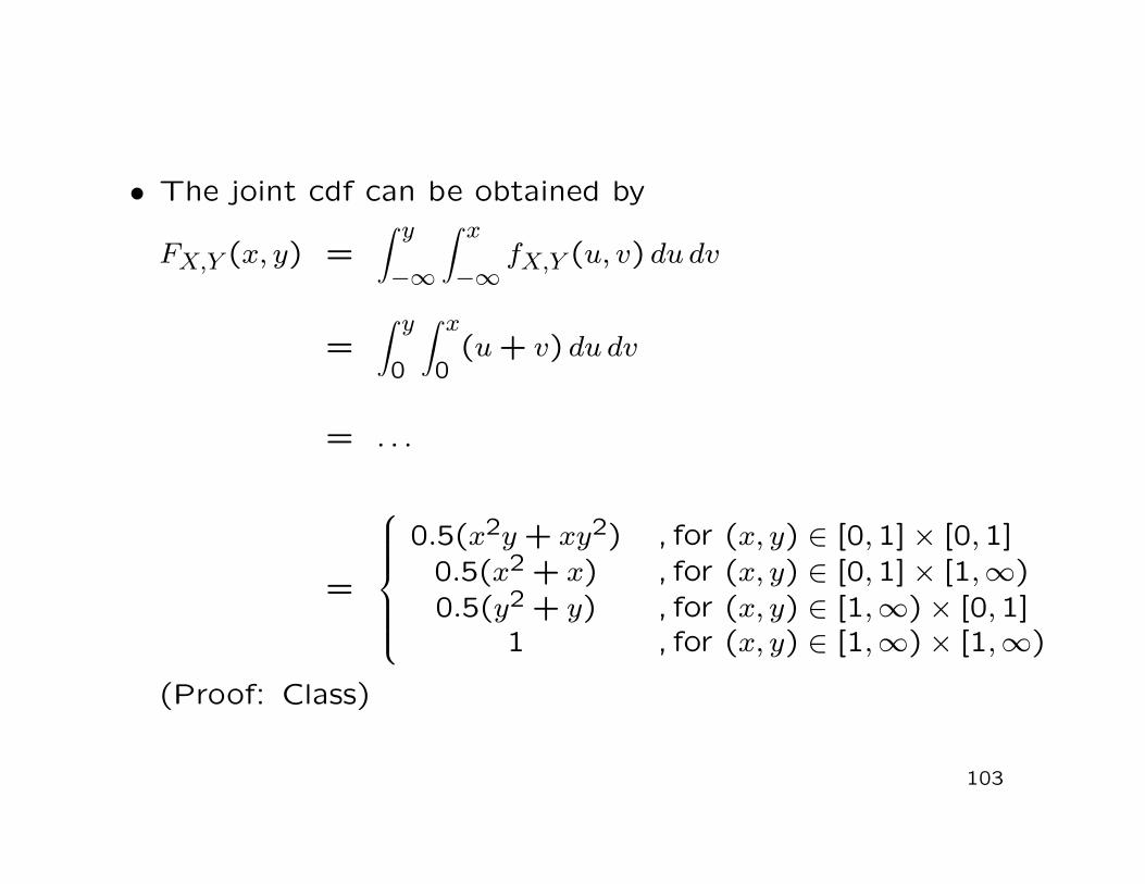
• The joint cdf can be obtained by

FX,Y (x, y) =∫ y

−∞

∫ x

−∞fX,Y (u, v) du dv

=∫ y

0

∫ x

0(u + v) du dv

= . . .

=

0.5(x2y + xy2) , for (x, y) ∈ [0,1]× [0,1]0.5(x2 + x) , for (x, y) ∈ [0,1]× [1,∞)0.5(y2 + y) , for (x, y) ∈ [1,∞)× [0,1]

1 , for (x, y) ∈ [1,∞)× [1,∞)

(Proof: Class)

103

Remarks:

• If X = (X1, . . . , Xn)′ is a joint continuous random vector,then

∂nFX1,...,Xn(x1, . . . , xn)

∂x1 · · · ∂xn= fX1,...,Xn(x1, . . . , xn)

• The volume under the joint pdf represents probabilities:

P (aL1 < X1 ≤ aU

1, . . . , aLn < Xn ≤ aU

n)

=∫ aU

n

aLn

. . .∫ aU

1

aL1

fX1,...,Xn(u1, . . . , un) du1 . . . dun

104

• In this course:

Emphasis on joint continuous random vectors

Analogous results for joint discrete random vectors(see Mood, Graybill, Boes (1974), Chapter IV)

Now:

• Determination of the distribution of a single random vari-able Xi from the joint distribution of the random vector(X1, . . . , Xn)′

−→ marginal distribution

105

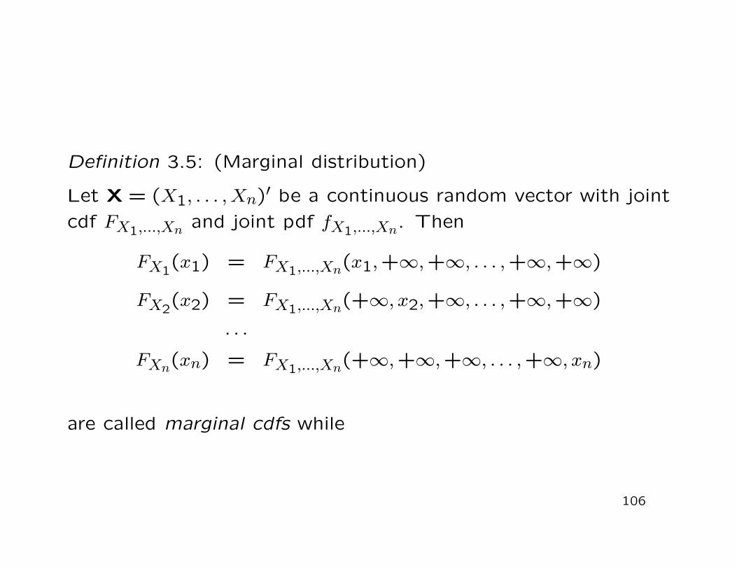
Definition 3.5: (Marginal distribution)

Let X = (X1, . . . , Xn)′ be a continuous random vector with jointcdf FX1,...,Xn and joint pdf fX1,...,Xn. Then

FX1(x1) = FX1,...,Xn(x1,+∞,+∞, . . . ,+∞,+∞)

FX2(x2) = FX1,...,Xn(+∞, x2,+∞, . . . ,+∞,+∞)

. . .

FXn(xn) = FX1,...,Xn(+∞,+∞,+∞, . . . ,+∞, xn)

are called marginal cdfs while

106

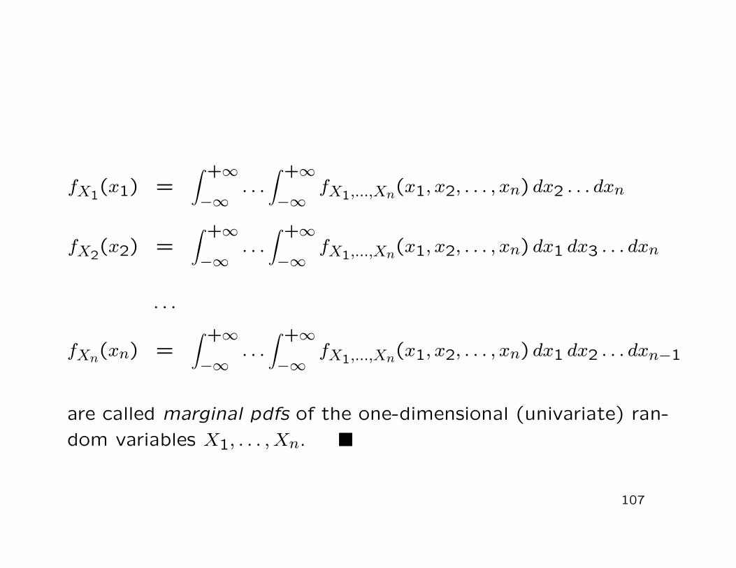
fX1(x1) =∫ +∞

−∞. . .

∫ +∞

−∞fX1,...,Xn(x1, x2, . . . , xn) dx2 . . . dxn

fX2(x2) =∫ +∞

−∞. . .

∫ +∞

−∞fX1,...,Xn(x1, x2, . . . , xn) dx1 dx3 . . . dxn

· · ·

fXn(xn) =∫ +∞

−∞. . .

∫ +∞

−∞fX1,...,Xn(x1, x2, . . . , xn) dx1 dx2 . . . dxn−1

are called marginal pdfs of the one-dimensional (univariate) ran-dom variables X1, . . . , Xn.

107

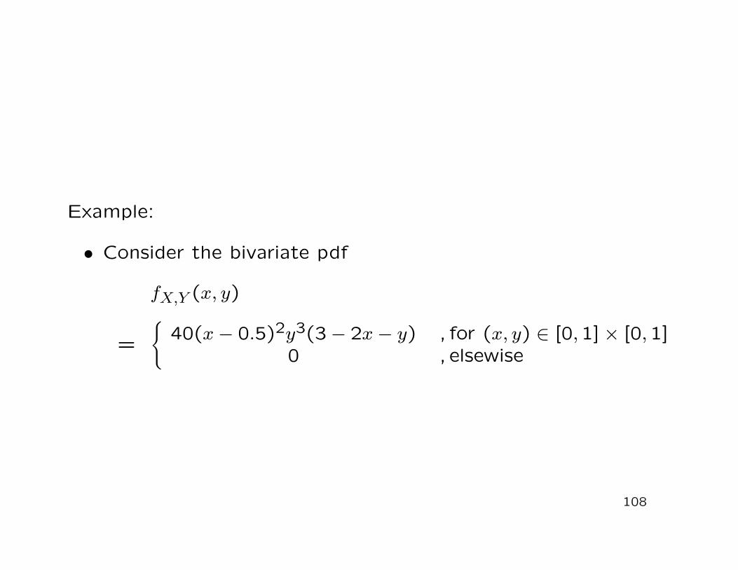
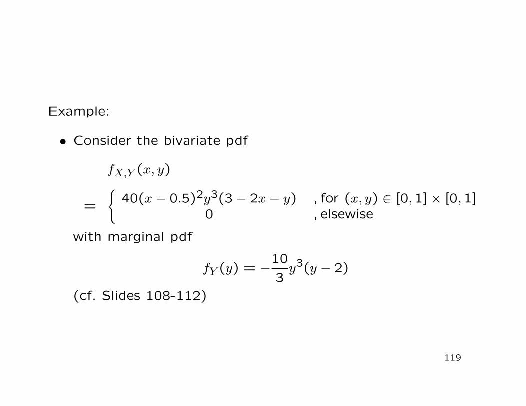
Example:

• Consider the bivariate pdf

fX,Y (x, y)

=

40(x− 0.5)2y3(3− 2x− y) , for (x, y) ∈ [0,1]× [0,1]0 , elsewise

108

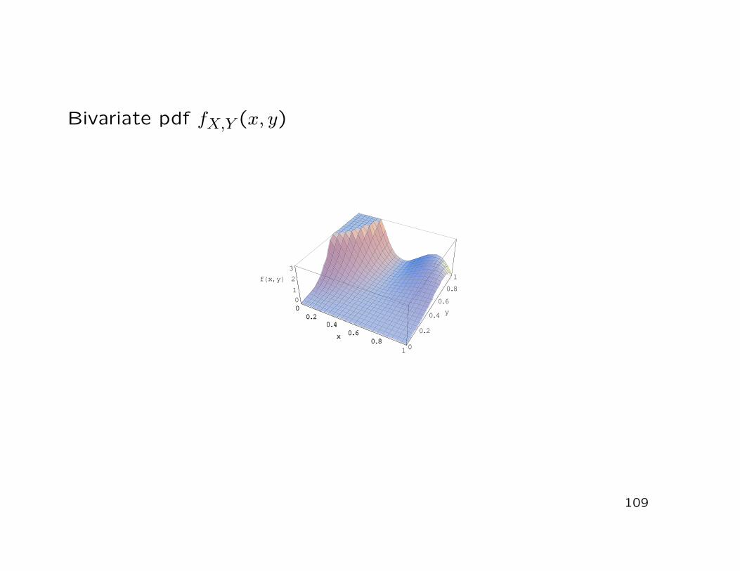
Bivariate pdf fX,Y (x, y)

109

00.2

0.40.6

0.81

x0

0.2

0.4

0.6

0.8

1

y

01

23

fHx,yL

00.2

0.40.6

0.8x

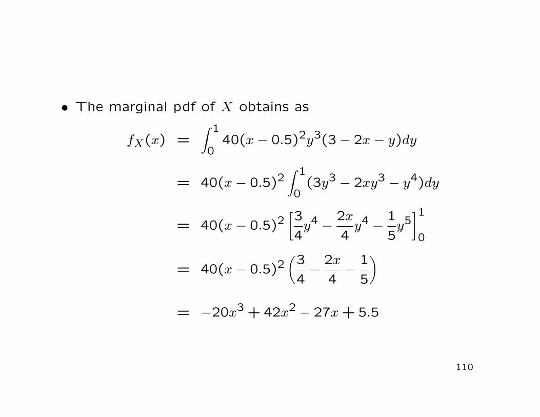
• The marginal pdf of X obtains as

fX(x) =∫ 1

040(x− 0.5)2y3(3− 2x− y)dy

= 40(x− 0.5)2∫ 1

0(3y3 − 2xy3 − y4)dy

= 40(x− 0.5)2[34

y4 −2x4

y4 −15

y5]1

0

= 40(x− 0.5)2(34−

2x4−

15

)

= −20x3 + 42x2 − 27x + 5.5

110

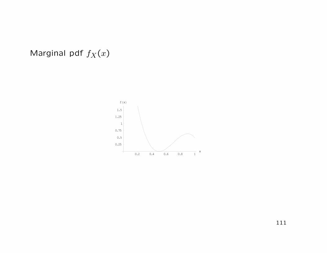
Marginal pdf fX(x)

111

0.2 0.4 0.6 0.8 1x

0.25

0.5

0.75

1

1.25

1.5

fHxL

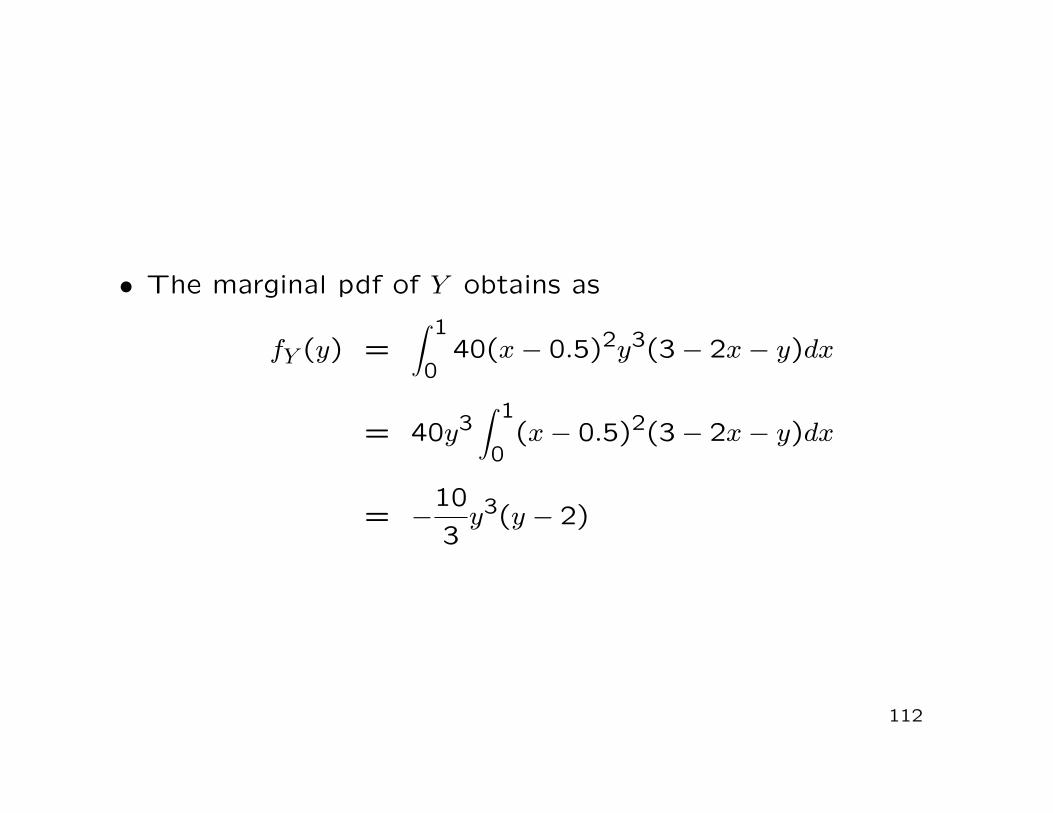
• The marginal pdf of Y obtains as

fY (y) =∫ 1

040(x− 0.5)2y3(3− 2x− y)dx

= 40y3∫ 1

0(x− 0.5)2(3− 2x− y)dx

= −103

y3(y − 2)

112

Marginal pdf fY (y)

113

0.2 0.4 0.6 0.8 1y

0.5

1

1.5

2

2.5

3

fHyL

Remarks:

• When considering the marginal instead of the joint distribu-tions, we are faced with an information loss(the joint distribution uniquely determines all marginal distri-butions, but the converse does not hold in general)

• Besides the respective univariate marginal distributions, thereare also multivariate distributions which can be obtained fromthe joint distribution of X = (X1, . . . , Xn)′

114

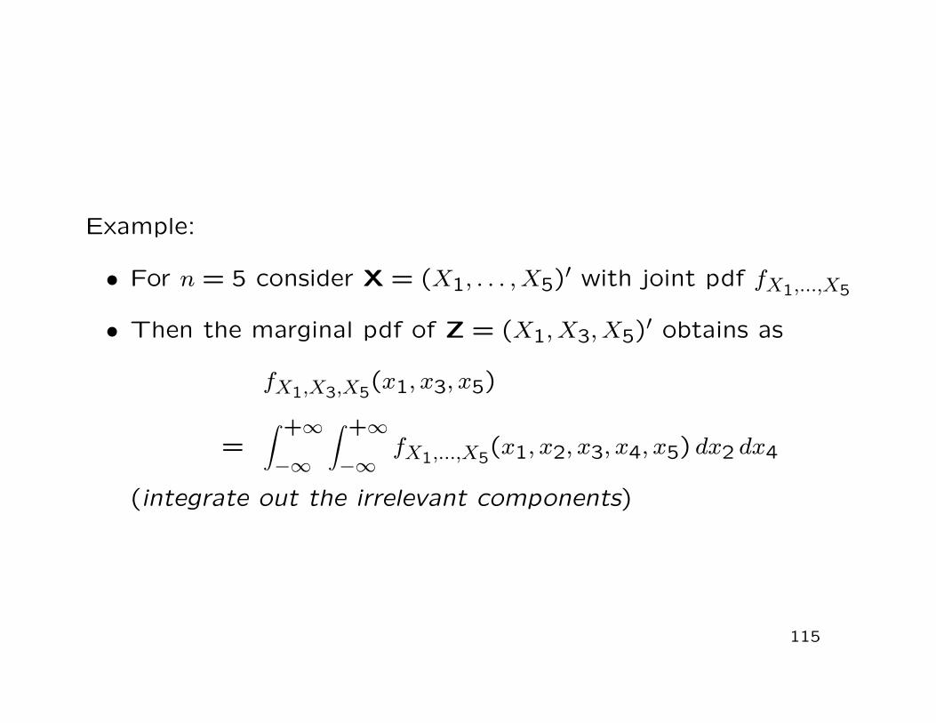
Example:

• For n = 5 consider X = (X1, . . . , X5)′ with joint pdf fX1,...,X5

• Then the marginal pdf of Z = (X1, X3, X5)′ obtains as

fX1,X3,X5(x1, x3, x5)

=∫ +∞

−∞

∫ +∞

−∞fX1,...,X5(x1, x2, x3, x4, x5) dx2 dx4

(integrate out the irrelevant components)

115

3.2 Conditional Distribution and Stochastic Inde-pendence

Now:

• Distribution of a random variable X under the condition thatanother random variable Y has already taken on the realiza-tion y(conditional distribution of X given Y = y)

116

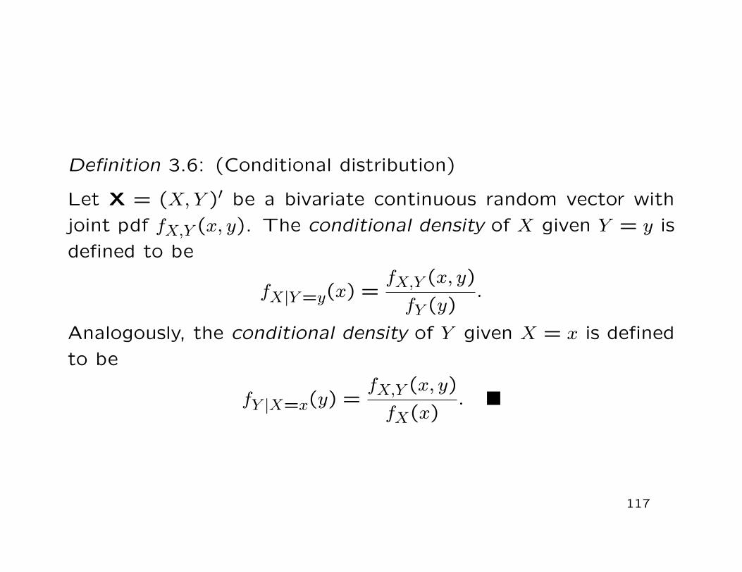
Definition 3.6: (Conditional distribution)

Let X = (X, Y )′ be a bivariate continuous random vector withjoint pdf fX,Y (x, y). The conditional density of X given Y = y isdefined to be

fX|Y =y(x) =fX,Y (x, y)

fY (y).

Analogously, the conditional density of Y given X = x is definedto be

fY |X=x(y) =fX,Y (x, y)

fX(x).

117

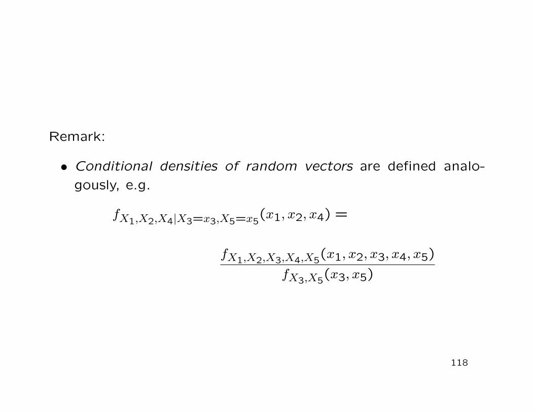
Remark:

• Conditional densities of random vectors are defined analo-gously, e.g.

fX1,X2,X4|X3=x3,X5=x5(x1, x2, x4) =

fX1,X2,X3,X4,X5(x1, x2, x3, x4, x5)

fX3,X5(x3, x5)

118

Example:

• Consider the bivariate pdf

fX,Y (x, y)

=

40(x− 0.5)2y3(3− 2x− y) , for (x, y) ∈ [0,1]× [0,1]0 , elsewise

with marginal pdf

fY (y) = −103

y3(y − 2)

(cf. Slides 108-112)

119

• It follows that

fX|Y =y(x) =fX,Y (x, y)

fY (y)

=40(x− 0.5)2y3(3− 2x− y)

−103 y3(y − 2)

=12(x− 0.5)2(3− 2x− y)

2− y

120

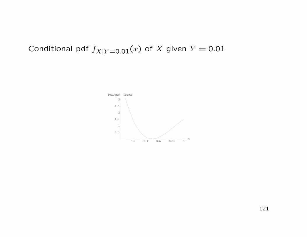
Conditional pdf fX|Y =0.01(x) of X given Y = 0.01

121

0.2 0.4 0.6 0.8 1x

0.5

1

1.5

2

2.5

3

Bedingte Dichte

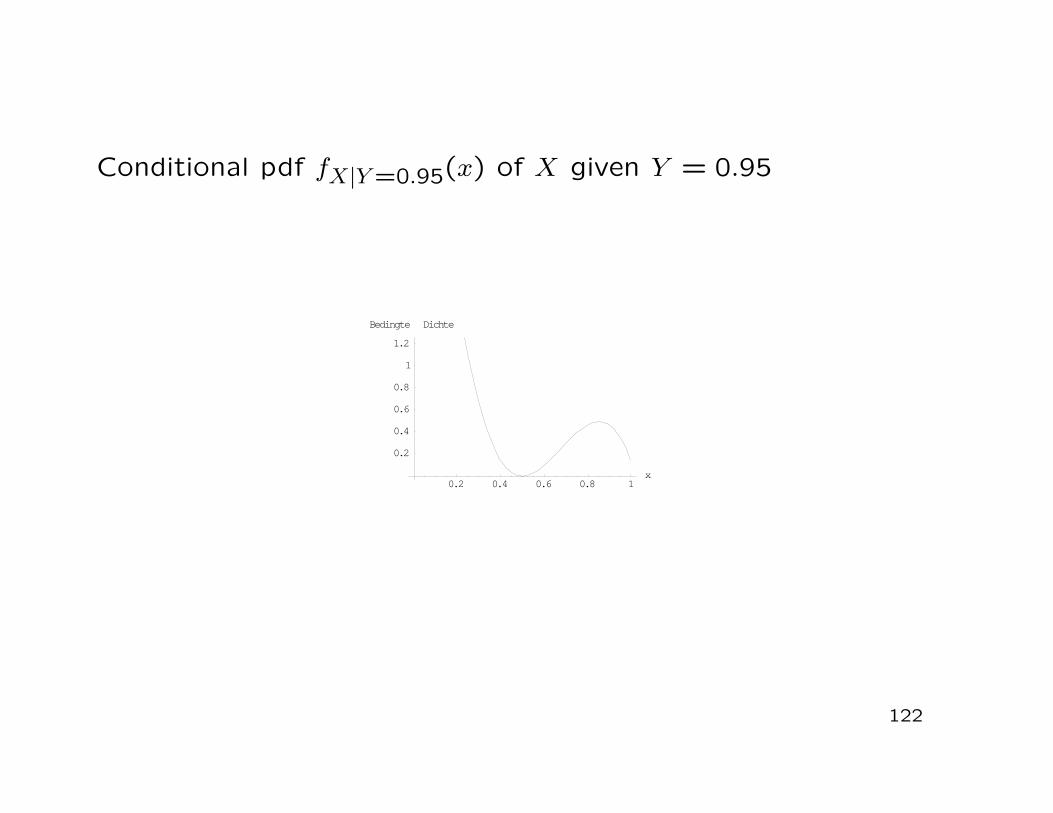
Conditional pdf fX|Y =0.95(x) of X given Y = 0.95

122

0.2 0.4 0.6 0.8 1x

0.2

0.4

0.6

0.8

1

1.2

Bedingte Dichte

Now:

• Combine the concepts ’joint distribution’ and ’conditionaldistribution’ to define the notion ’stochastic independence’(for two random variables first)

Definition 3.7: (Stochastic Independence [I])

Let (X, Y )′ be a bivariate continuous random vector with jointpdf fX,Y (x, y). X and Y are defined to be stochastically inde-pendent if and only if

fX,Y (x, y) = fX(x) · fY (y) for all x, y ∈ R.

123

Remarks:

• Alternatively, stochastic independence can be defined via thecdfs:X and Y are stochastically independent, if and only if

FX,Y (x, y) = FX(x) · FY (y) for all x, y ∈ R.

• If X and Y are independent, we have

fX|Y =y(x) =fX,Y (x, y)

fY (y)=

fX(x) · fY (y)fY (y)

= fX(x)

fY |X=x(y) =fX,Y (x, y)

fX(x)=

fX(x) · fY (y)fX(x)

= fY (y)

• If X and Y are independent and g and h are two continuousfunctions, then g(X) and h(Y ) are also independent

124

Now:

• Extension to n random variables

Definition 3.8: (Stochastic independence [II])

Let (X1, . . . , Xn)′ be a continuous random vector with joint pdffX1,...,Xn(x1, . . . , xn) and joint cdf FX1,...,Xn(x1, . . . , xn). X1, . . . , Xn

are defined to be stochastically independent, if and only if for all(x1, . . . , xn)′ ∈ Rn

fX1,...,Xn(x1, . . . , xn) = fX1(x1) · . . . · fXn(xn)

or

FX1,...,Xn(x1, . . . , xn) = FX1(x1) · . . . · FXn(xn).

125

Remarks:

• For discrete random vectors we define: X1, . . . , Xn are stochas-tically independent, if and only if for all (x1, . . . , xn)′ ∈ Rn

P (X1 = x1, . . . , Xn = xn) = P (X1 = x1) · . . . · P (Xn = xn)

or

FX1,...,Xn(x1, . . . , xn) = FX1(x1) · . . . · FXn(xn)

• In the case of independence, the joint distribution resultsfrom the marginal distributions

• If X1, . . . , Xn are stochastically independent and g1, . . . , gn arecontinuous functions, then Y1 = g1(X1), . . . , Yn = gn(Xn) arealso stochastically independent

126

3.3 Expectation and Joint Moment GeneratingFunctions

Now:

• Definition of the expectation of a function

g : Rn −→ R(x1, . . . , xn) 7−→ g(x1, . . . xn)

of a continuous random vector X = (X1, . . . , Xn)′

127

Definition 3.9: (Expectation of a function)

Let (X1, . . . , Xn)′ be a continuous random vector with joint pdffX1,...,Xn(x1, . . . , xn) and g : Rn −→ R a real-valued continuousfunction. The expectation of the function g of the random vectoris defined to be

E[g(X1, . . . , Xn)]

=∫ +∞

−∞. . .

∫ +∞

−∞g(x1, . . . , xn) · fX1,...,Xn(x1, . . . , xn) dx1 . . . dxn.

128

Remarks:

• For a discrete random vector (X1, . . . , Xn)′ the analogous def-inition is

E[g(X1, . . . , Xn)] =∑

g(x1, . . . , xn) · P (X1 = x1, . . . , Xn = xn),

where the summation is over all realizationen of the vector

• Definition 3.9 includes the expectation of a univariate ran-dom variable X:Set n = 1 and g(x) = x

−→ E(X1) ≡ E(X) =∫ +∞

−∞xfX(x) dx

• Definition 3.9 includes the variance of X:Set n = 1 and g(x) = [x− E(X)]2

−→ Var(X1) ≡ Var(X) =∫ +∞

−∞[x− E(X)]2fX(x) dx

129

• Definition 3.9 includes the covariance of two variables:Set n = 2 and g(x1, x2) = [x1 − E(X1)] · [x2 − E(X2)]

−→ Cov(X1, X2)

=∫ +∞

−∞

∫ +∞

−∞[x1 − E(X1)][x2 − E(X2)]fX1,X2(x1, x2) dx1 dx2

• Via the covariance we define the correlation coefficient:

Corr(X1, X2) =Cov(X1, X2)

√

Var(X1)√

Var(X2)

• General properties of expected values, variances, covariancesand the correlation coefficient−→ Class

130

Now:

• ’Expectation’ and ’variances’ of random vectors

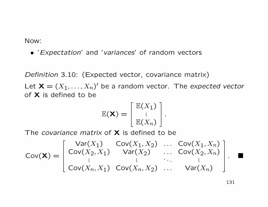
Definition 3.10: (Expected vector, covariance matrix)

Let X = (X1, . . . , Xn)′ be a random vector. The expected vectorof X is defined to be

E(X) =

E(X1)...

E(Xn)

.

The covariance matrix of X is defined to be

Cov(X) =

Var(X1) Cov(X1, X2) . . . Cov(X1, Xn)Cov(X2, X1) Var(X2) . . . Cov(X2, Xn)

... ... . . . ...Cov(Xn, X1) Cov(Xn, X2) . . . Var(Xn)

.

131

Remark:

• Obviously, the covariance matrix is symmetric per definition

Now:

• Expected vectors and covariance matrices under linear trans-formations of random vectors

Let

• X = (X1, . . . , Xn)′ be a n-dimensional random vector

• A be an (m× n) matrix of real numbers

• b be an (m× 1) column vector of real numbers

132

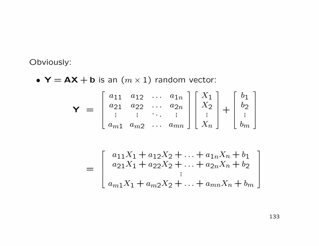
Obviously:

• Y = AX + b is an (m× 1) random vector:

Y =

a11 a12 . . . a1na21 a22 . . . a2n... ... . . . ...

am1 am2 . . . amn

X1X2...

Xn

+

b1b2...

bm

=

a11X1 + a12X2 + . . . + a1nXn + b1a21X1 + a22X2 + . . . + a2nXn + b2

...am1X1 + am2X2 + . . . + amnXn + bm

133

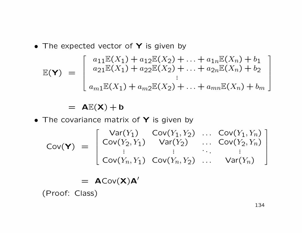
• The expected vector of Y is given by

E(Y) =

a11E(X1) + a12E(X2) + . . . + a1nE(Xn) + b1a21E(X1) + a22E(X2) + . . . + a2nE(Xn) + b2

...am1E(X1) + am2E(X2) + . . . + amnE(Xn) + bm

= AE(X) + b

• The covariance matrix of Y is given by

Cov(Y) =

Var(Y1) Cov(Y1, Y2) . . . Cov(Y1, Yn)Cov(Y2, Y1) Var(Y2) . . . Cov(Y2, Yn)

... ... . . . ...Cov(Yn, Y1) Cov(Yn, Y2) . . . Var(Yn)

= ACov(X)A′

(Proof: Class)

134

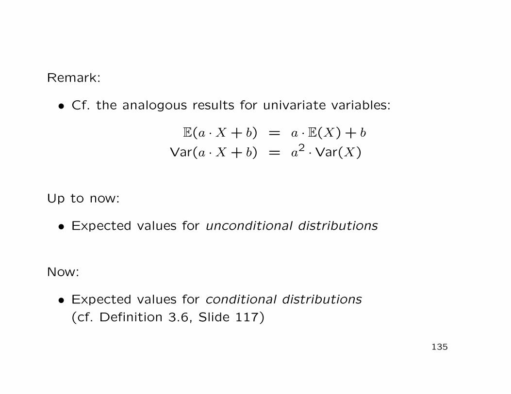
Remark:

• Cf. the analogous results for univariate variables:

E(a ·X + b) = a · E(X) + b

Var(a ·X + b) = a2 ·Var(X)

Up to now:

• Expected values for unconditional distributions

Now:

• Expected values for conditional distributions(cf. Definition 3.6, Slide 117)

135

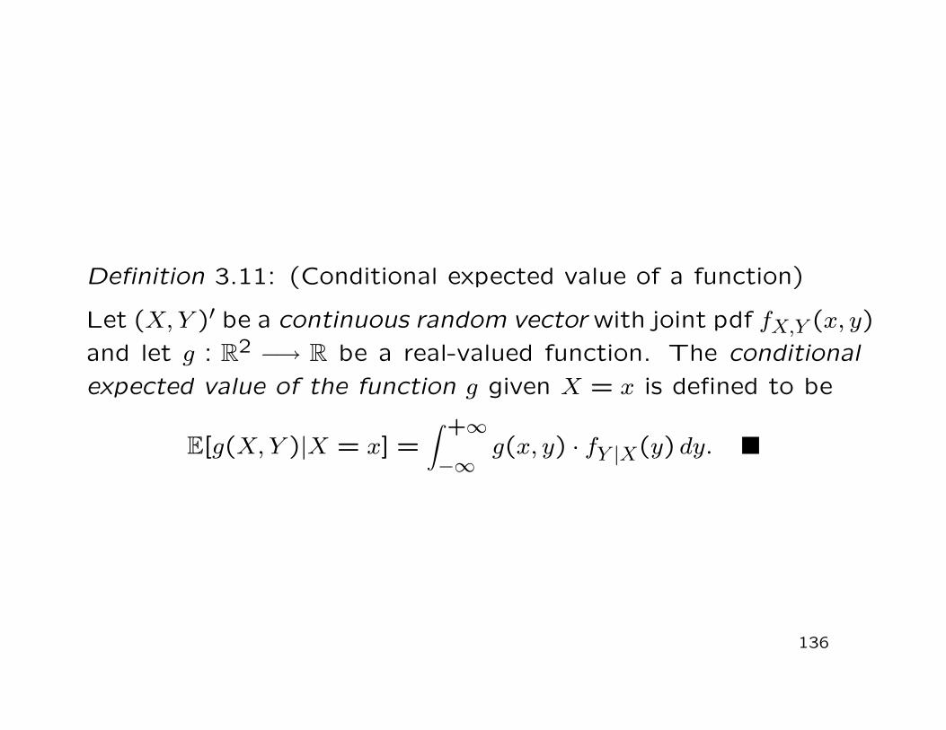
Definition 3.11: (Conditional expected value of a function)

Let (X, Y )′ be a continuous random vector with joint pdf fX,Y (x, y)and let g : R2 −→ R be a real-valued function. The conditionalexpected value of the function g given X = x is defined to be

E[g(X, Y )|X = x] =∫ +∞

−∞g(x, y) · fY |X(y) dy.

136

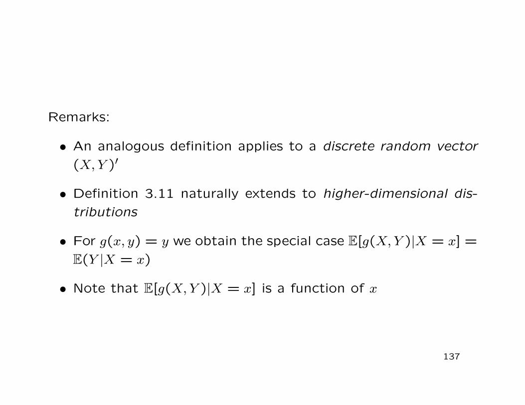
Remarks:

• An analogous definition applies to a discrete random vector(X, Y )′

• Definition 3.11 naturally extends to higher-dimensional dis-tributions

• For g(x, y) = y we obtain the special case E[g(X, Y )|X = x] =E(Y |X = x)

• Note that E[g(X, Y )|X = x] is a function of x

137

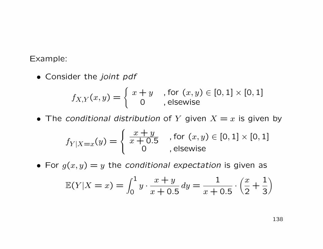
Example:

• Consider the joint pdf

fX,Y (x, y) =

x + y , for (x, y) ∈ [0,1]× [0,1]0 , elsewise

• The conditional distribution of Y given X = x is given by

fY |X=x(y) =

x + yx + 0.5 , for (x, y) ∈ [0,1]× [0,1]

0 , elsewise

• For g(x, y) = y the conditional expectation is given as

E(Y |X = x) =∫ 1

0y ·

x + yx + 0.5

dy =1

x + 0.5·(x2

+13

)

138

Remarks:

• Consider the function g(x, y) = g(y)(i.e. g does not depend on x)

• Denote h(x) = E[g(Y )|X = x]

• We calculate the unconditional expectation of the trans-formed variable h(X)

• We have

139

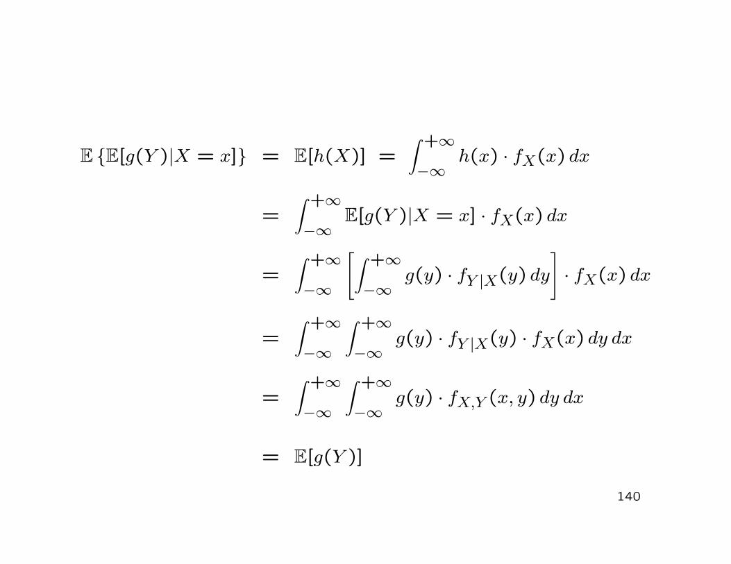
E E[g(Y )|X = x] = E[h(X)] =∫ +∞

−∞h(x) · fX(x) dx

=∫ +∞

−∞E[g(Y )|X = x] · fX(x) dx

=∫ +∞

−∞

[

∫ +∞

−∞g(y) · fY |X(y) dy

]

· fX(x) dx

=∫ +∞

−∞

∫ +∞

−∞g(y) · fY |X(y) · fX(x) dy dx

=∫ +∞

−∞

∫ +∞

−∞g(y) · fX,Y (x, y) dy dx

= E[g(Y )]

140

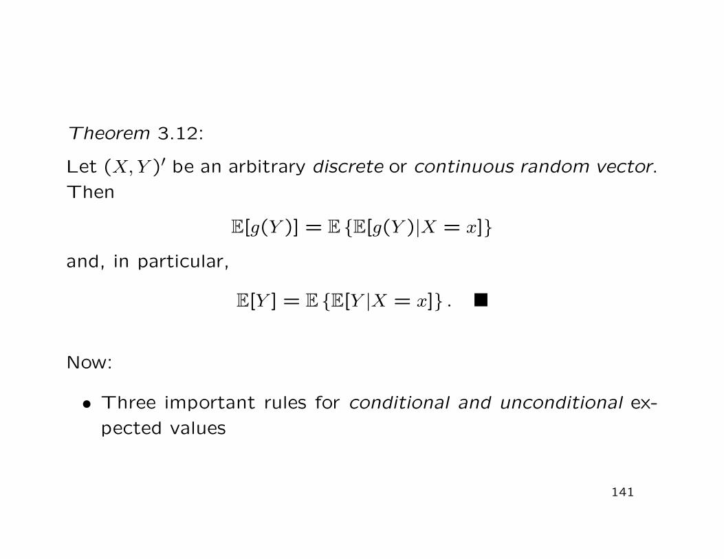
Theorem 3.12:

Let (X, Y )′ be an arbitrary discrete or continuous random vector.Then

E[g(Y )] = E E[g(Y )|X = x]

and, in particular,

E[Y ] = E E[Y |X = x] .

Now:

• Three important rules for conditional and unconditional ex-pected values

141

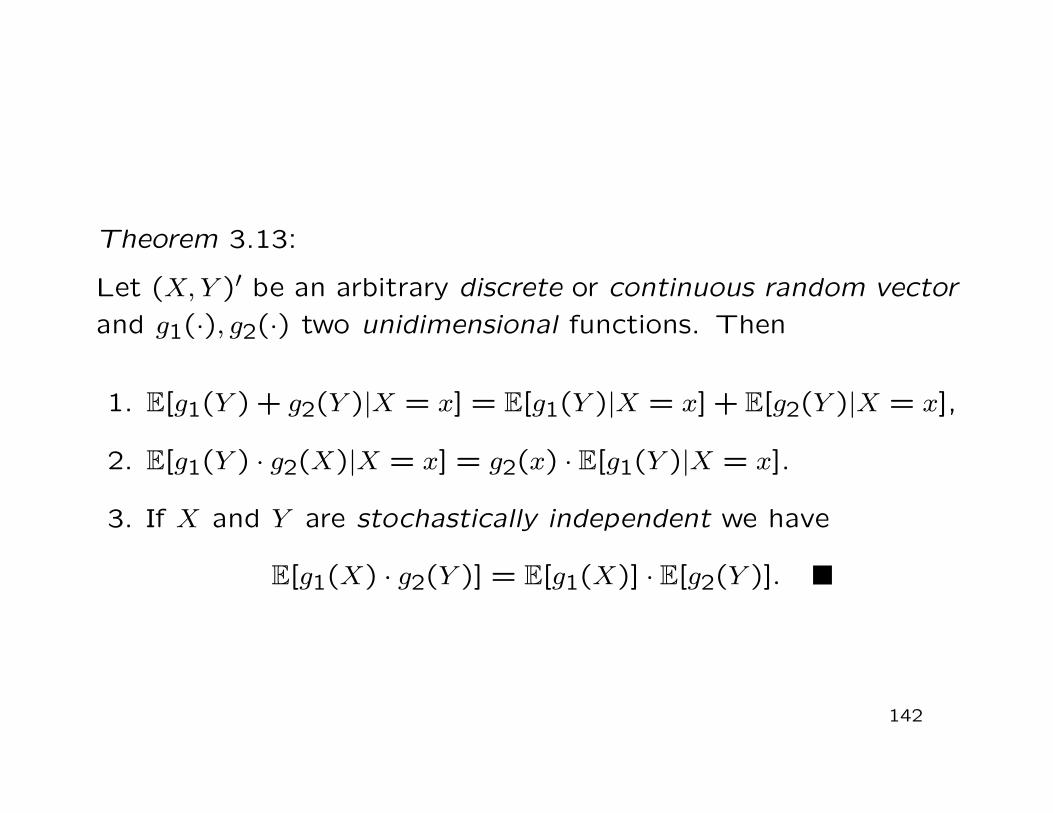
Theorem 3.13:

Let (X, Y )′ be an arbitrary discrete or continuous random vectorand g1(·), g2(·) two unidimensional functions. Then

1. E[g1(Y ) + g2(Y )|X = x] = E[g1(Y )|X = x] + E[g2(Y )|X = x],

2. E[g1(Y ) · g2(X)|X = x] = g2(x) · E[g1(Y )|X = x].

3. If X and Y are stochastically independent we have

E[g1(X) · g2(Y )] = E[g1(X)] · E[g2(Y )].

142

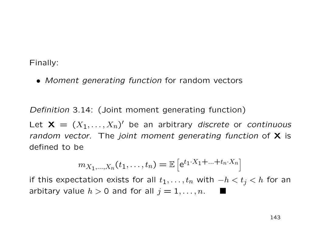
Finally:

• Moment generating function for random vectors

Definition 3.14: (Joint moment generating function)

Let X = (X1, . . . , Xn)′ be an arbitrary discrete or continuousrandom vector. The joint moment generating function of X isdefined to be

mX1,...,Xn(t1, . . . , tn) = E[

et1·X1+...+tn·Xn]

if this expectation exists for all t1, . . . , tn with −h < tj < h for anarbitary value h > 0 and for all j = 1, . . . , n.

143

Remarks:

• Via the joint moment generating function mX1,...,Xn(t1, . . . , tn)we can derive the following mathematical objects:

the marginal moment generating functions mX1(t1), . . . ,mXn(tn)

the moments of the marginal distributions

the so-called joint moments

144

Important result: (cf. Theorem 2.23, Slide 85)

For any given joint moment generating functionmX1,...,Xn(t1, . . . , tn) there exists a unique joint cdfFX1,...,Xn(x1, . . . , xn)

145

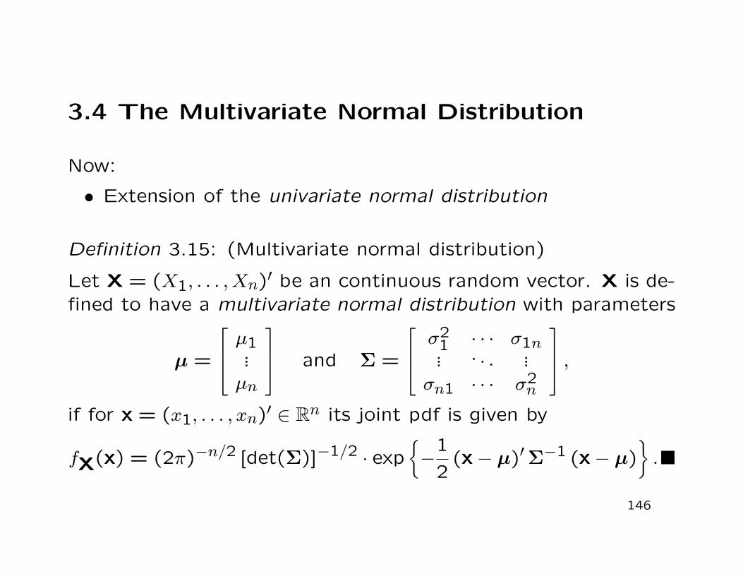
3.4 The Multivariate Normal Distribution

Now:

• Extension of the univariate normal distribution

Definition 3.15: (Multivariate normal distribution)

Let X = (X1, . . . , Xn)′ be an continuous random vector. X is de-fined to have a multivariate normal distribution with parameters

µ =

µ1...

µn

and Σ =

σ21 · · · σ1n... . . . ...

σn1 · · · σ2n

,

if for x = (x1, . . . , xn)′ ∈ Rn its joint pdf is given by

fX(x) = (2π)−n/2 [det(Σ)]−1/2 · exp

−12

(x− µ)′Σ−1 (x− µ)

.

146

Remarks:

• See Chang (1984, p. 92) for a definition and the propertiesof the determinant det(A) of the matrix A

• Notation:

X ∼ N(µ,Σ)

• µ is a column vector with µ1, . . . , µn ∈ R

• Σ is a regular, positive definite, symmetric (n× n) matrix

• Role of the parameters:

E(X) = µ and Cov(X) = Σ

147

• Joint pdf of the multiv. standard normal distribution N(0, In):

φ(x) = (2π)−n/2 · exp

−12x′x

• Cf. the analogy to the univariate pdf in Definition 2.24, Slide91

Properties of the N(µ,Σ) distribution:

• Partial vectors (marginal distributions) of X also have multi-variate normal distributions, i.e. if

X =

[

X1X2

]

∼ N

([

µ1µ2

]

,

[

Σ11 Σ12Σ21 Σ22

])

then

X1 ∼ N(µ1,Σ11)X2 ∼ N(µ2,Σ22)

148

• Thus, all univariate variables of X = (X1, . . . , Xn)′ have uni-variate normal distributions:

X1 ∼ N(µ1, σ21)

X2 ∼ N(µ2, σ22)

...Xn ∼ N(µn, σ2

n)

• The conditional distributions are also (univariately or multi-variately) normal:

X1|X2 = x2 ∼ N(

µ1 + Σ12Σ−122 (x2 − µ2),Σ11 −Σ12Σ

−122 Σ21

)

• Linear transformations:Let A be an (m × n) matrix, b an (m × 1) vector of realnumbers and X = (X1, . . . , Xn)′ ∼ N(µ,Σ). Then

AX + b ∼ N(Aµ + b,AΣA′)

149

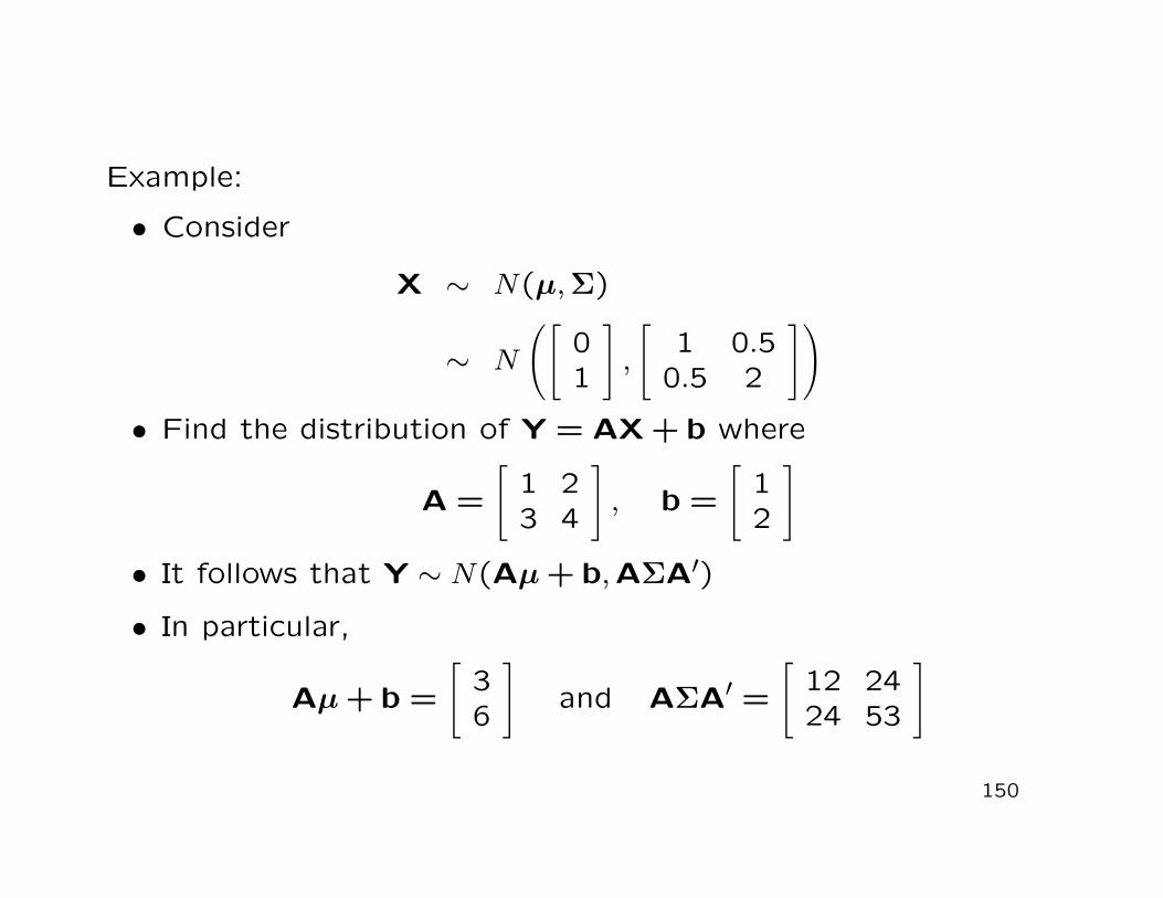
Example:

• Consider

X ∼ N(µ,Σ)

∼ N

([

01

]

,

[

1 0.50.5 2

])

• Find the distribution of Y = AX + b where

A =

[

1 23 4

]

, b =

[

12

]

• It follows that Y ∼ N(Aµ + b,AΣA′)

• In particular,

Aµ + b =

[

36

]

and AΣA′ =

[

12 2424 53

]

150

Now:

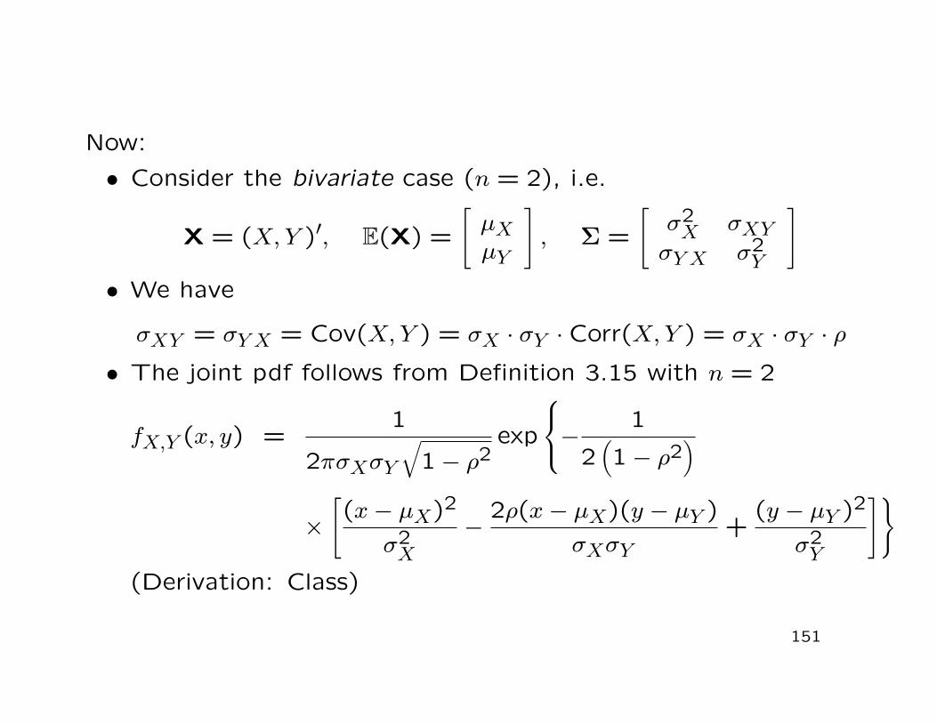
• Consider the bivariate case (n = 2), i.e.

X = (X, Y )′, E(X) =

[

µXµY

]

, Σ =

[

σ2X σXY

σY X σ2Y

]

• We have

σXY = σY X = Cov(X, Y ) = σX · σY ·Corr(X, Y ) = σX · σY · ρ• The joint pdf follows from Definition 3.15 with n = 2

fX,Y (x, y) =1

2πσXσY

√

1− ρ2exp

−1

2(

1− ρ2)

×[

(x− µX)2

σ2X

−2ρ(x− µX)(y − µY )

σXσY+

(y − µY )2

σ2Y

]

(Derivation: Class)

151

fX,Y (x, y) for µX = µY = 0, σx = σY = 1 and ρ = 0

152

-2

0

2x -2

0

2

y

00.05

0.1

0.15

fHx,yL

-2

0

2x

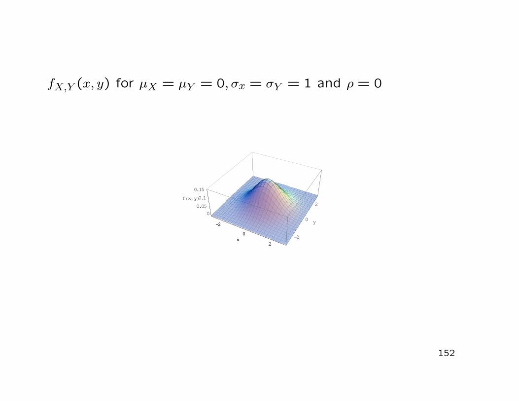
fX,Y (x, y) for µX = µY = 0, σx = σY = 1 and ρ = 0.9

153

-2

0

2x -2

0

2

y

00.1

0.2

0.3fHx,yL

-2

0

2x

Remarks:

• The marginal distributions are given by

X ∼ N(µX , σ2X) and Y ∼ N(µY , σ2

Y )−→ interesting result for the normal distribution:

If (X, Y )′ has a bivariate normal distribution, then X and Yare independent if and only if ρ = Corr(X, Y ) = 0

• The conditional distributions are given by

X|Y = y ∼ N

(

µX + ρσXσY

(y − µY ), σ2X

(

1− ρ2)

)

Y |X = x ∼ N

(

µY + ρσYσX

(x− µX), σ2Y

(

1− ρ2)

)

(Proof: Class)

154

4. Distributions of Functions of Random Vari-ables

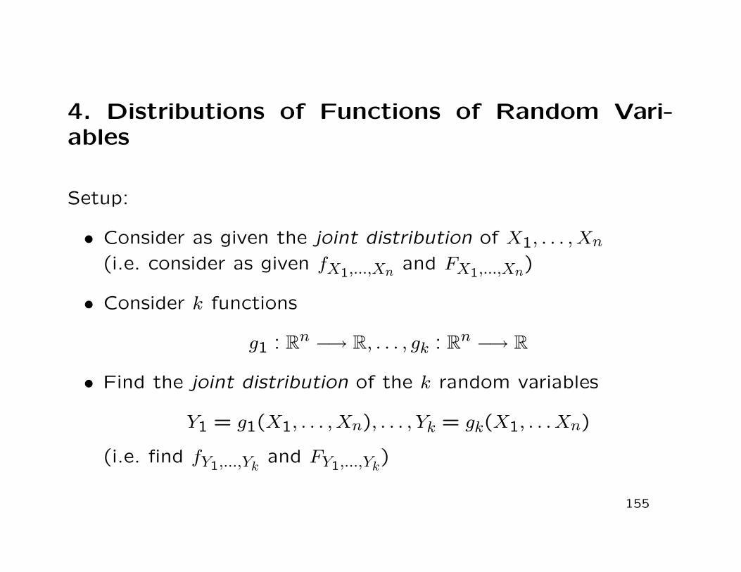
Setup:

• Consider as given the joint distribution of X1, . . . , Xn

(i.e. consider as given fX1,...,Xn and FX1,...,Xn)

• Consider k functions

g1 : Rn −→ R, . . . , gk : Rn −→ R

• Find the joint distribution of the k random variables

Y1 = g1(X1, . . . , Xn), . . . , Yk = gk(X1, . . . Xn)

(i.e. find fY1,...,Ykand FY1,...,Yk

)

155

Example:

• Consider as given X1, . . . , Xn with fX1,...,Xn

• Consider the functions

g1(X1, . . . , Xn) =n

∑

i=1Xi and g2(X1, . . . , Xn) =

1n

n∑

i=1Xi

• Find fY1,Y2 with Y1 =∑n

i=1 Xi and Y2 = 1n

∑ni=1 Xi

Remark:

• From the joint distribution fY1,...,Ykwe can derive the k marginal

distributions fY1, . . . fYk(cf. Chapter 3, Slides 106, 107)

156

Aim of this chapter:

• Techniques for finding the (marginal) distribution(s)of (Y1, . . . , Yk)

′

157

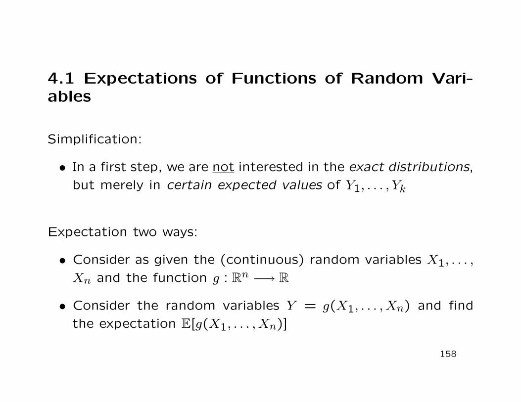
4.1 Expectations of Functions of Random Vari-ables

Simplification:

• In a first step, we are not interested in the exact distributions,but merely in certain expected values of Y1, . . . , Yk

Expectation two ways:

• Consider as given the (continuous) random variables X1, . . . ,Xn and the function g : Rn −→ R

• Consider the random variables Y = g(X1, . . . , Xn) and findthe expectation E[g(X1, . . . , Xn)]

158

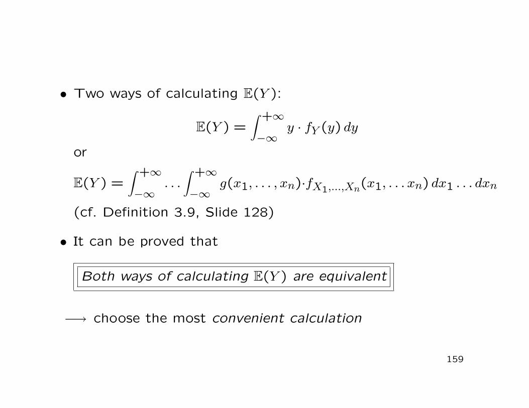
• Two ways of calculating E(Y ):

E(Y ) =∫ +∞

−∞y · fY (y) dy

or

E(Y ) =∫ +∞

−∞. . .

∫ +∞

−∞g(x1, . . . , xn)·fX1,...,Xn(x1, . . . xn) dx1 . . . dxn

(cf. Definition 3.9, Slide 128)

• It can be proved that

Both ways of calculating E(Y ) are equivalent

−→ choose the most convenient calculation

159

Now:

• Calculation rules for expected values, variances, covariancesof sums of random variables

Setting:

• X1, . . . , Xn are given continuous or discrete random variableswith joint density fX1,...,Xn

• The (transforming) function g : Rn −→ R is given by

g(x1, . . . , xn) =n

∑

i=1xi

160

• In a first step, find the expectation and the variance of

Y = g(X1, . . . , Xn) =n

∑

i=1Xi

Theorem 4.1: (Expectation and variance of a sum)

For the given random variables X1, . . . , Xn we have

E

n∑

i=1Xi

=n

∑

i=1E(Xi)

and

Var

n∑

i=1Xi

=n

∑

i=1Var(Xi) + 2 ·

n∑

i=1

n∑

j=i+1Cov(Xi, Xj).

161

Implications:

• For given constants a1, . . . , an ∈ R we have

E

n∑

i=1ai ·Xi

=n

∑

i=1ai · E(Xi)

(why?)

• For two random variables X1 and X2 we have

E(X1 ±X2) = E(X1)± E(X2)

• If X1, . . . , Xn are stochastically independent, it follows thatCov(Xi, Xj) = 0 for all i 6= j and hence

Var

n∑

i=1Xi

=n

∑

i=1Var(Xi)

162

Now:

• Calculating the covariance of two sums of random variables

Theorem 4.2: (Covariance of two sums)

Let X1, . . . , Xn and Y1, . . . , Ym be two sets of random variablesand let a1, . . . an and b1, . . . , bm be two sets of constants. Then

Cov

n∑

i=1ai ·Xi,

m∑

j=1bj · Yj

=n

∑

i=1

m∑

j=1ai · bj ·Cov(Xi, Yj).

163

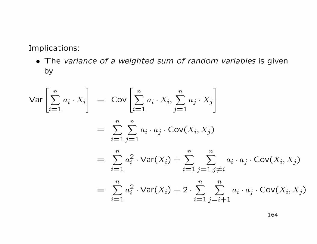
Implications:

• The variance of a weighted sum of random variables is givenby

Var

n∑

i=1ai ·Xi

= Cov

n∑

i=1ai ·Xi,

n∑

j=1aj ·Xj

=n

∑

i=1

n∑

j=1ai · aj ·Cov(Xi, Xj)

=n

∑

i=1a2

i ·Var(Xi) +n

∑

i=1

n∑

j=1,j 6=iai · aj ·Cov(Xi, Xj)

=n

∑

i=1a2

i ·Var(Xi) + 2 ·n

∑

i=1

n∑

j=i+1ai · aj ·Cov(Xi, Xj)

164

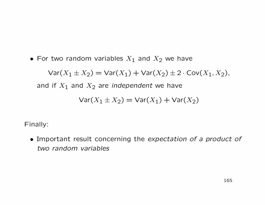
• For two random variables X1 and X2 we have

Var(X1 ±X2) = Var(X1) + Var(X2)± 2 ·Cov(X1, X2),

and if X1 and X2 are independent we have

Var(X1 ±X2) = Var(X1) + Var(X2)

Finally:

• Important result concerning the expectation of a product oftwo random variables

165

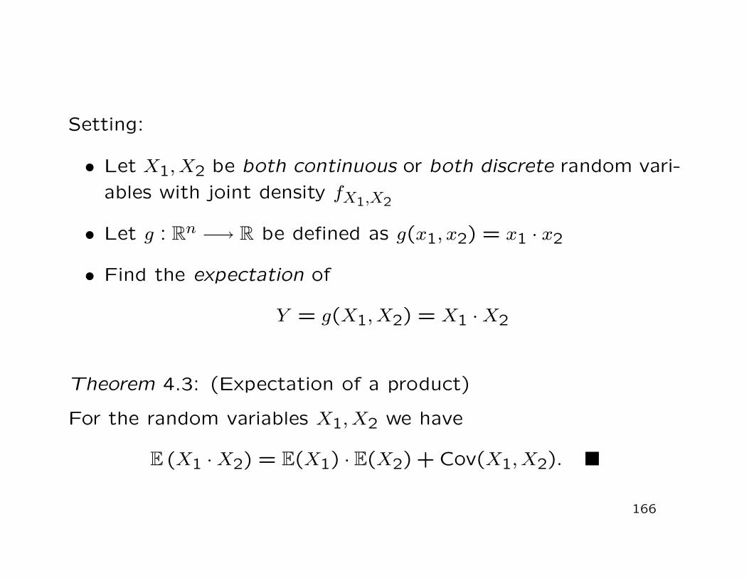
Setting:

• Let X1, X2 be both continuous or both discrete random vari-ables with joint density fX1,X2

• Let g : Rn −→ R be defined as g(x1, x2) = x1 · x2

• Find the expectation of

Y = g(X1, X2) = X1 ·X2

Theorem 4.3: (Expectation of a product)

For the random variables X1, X2 we have

E (X1 ·X2) = E(X1) · E(X2) + Cov(X1, X2).

166

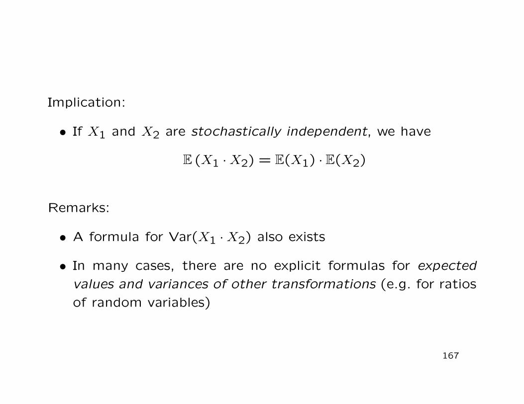
Implication:

• If X1 and X2 are stochastically independent, we have

E (X1 ·X2) = E(X1) · E(X2)

Remarks:

• A formula for Var(X1 ·X2) also exists

• In many cases, there are no explicit formulas for expectedvalues and variances of other transformations (e.g. for ratiosof random variables)

167

4.2 The Cumulative-distribution-function Tech-nique

Motivation:

• Consider as given the random variables X1, . . . , Xn with jointdensity fX1,...,Xn

• Find the joint distribution of Y1, . . . , Yk where Yj = gj(X1, . . . ,Xn) for j = 1, . . . , k

• The joint cdf of Y1, . . . , Yk is defined to be

FY1,...,Yk(y1, . . . , yk) = P (Y1 ≤ y1, . . . , Yk ≤ yk)

(cf. Definition 3.2, Slide 98)

168

• Now, for each y1, . . . , yk the event

Y1 ≤ y1, . . . , Yk ≤ yk

= g1(X1, . . . , Xn) ≤ y1, . . . , gk(X1, . . . , Xn) ≤ yk ,

i.e. the latter event is an event described in terms of the givenfunctions g1, . . . , gk and the given random variables X1, . . . , Xn

−→ since the joint distribution of X1, . . . , Xn is assumed given,presumably the probability of the latter event can be cal-culated and consequently FY1,...,Yk

determined

169

Example 1:

• Consider n = 1 (i.e. consider X1 ≡ X with cdf FX) and k = 1(i.e. g1 ≡ g and Y1 ≡ Y )

• Consider the function

g(x) = a · x + b, b ∈ R, a > 0

• Find the distribution of

Y = g(X) = a ·X + b

170

• The cdf of Y is given by

FY (y) = P (Y ≤ y)

= P [g(X) ≤ y]

= P (a ·X + b ≤ y)

= P(

X ≤y − b

a

)

= FX

(y − ba

)

• If X is continuous, the pdf of Y is given by

fY (y) = F ′Y (y) = F ′X

(y − ba

)

=1a· fX

(y − ba

)

(cf. Slide 48)

171

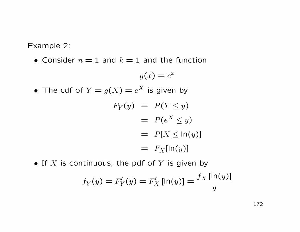
Example 2:

• Consider n = 1 and k = 1 and the function

g(x) = ex

• The cdf of Y = g(X) = eX is given by

FY (y) = P (Y ≤ y)

= P (eX ≤ y)

= P [X ≤ ln(y)]

= FX[ln(y)]

• If X is continuous, the pdf of Y is given by

fY (y) = F ′Y (y) = F ′X [ln(y)] =fX [ln(y)]

y

172

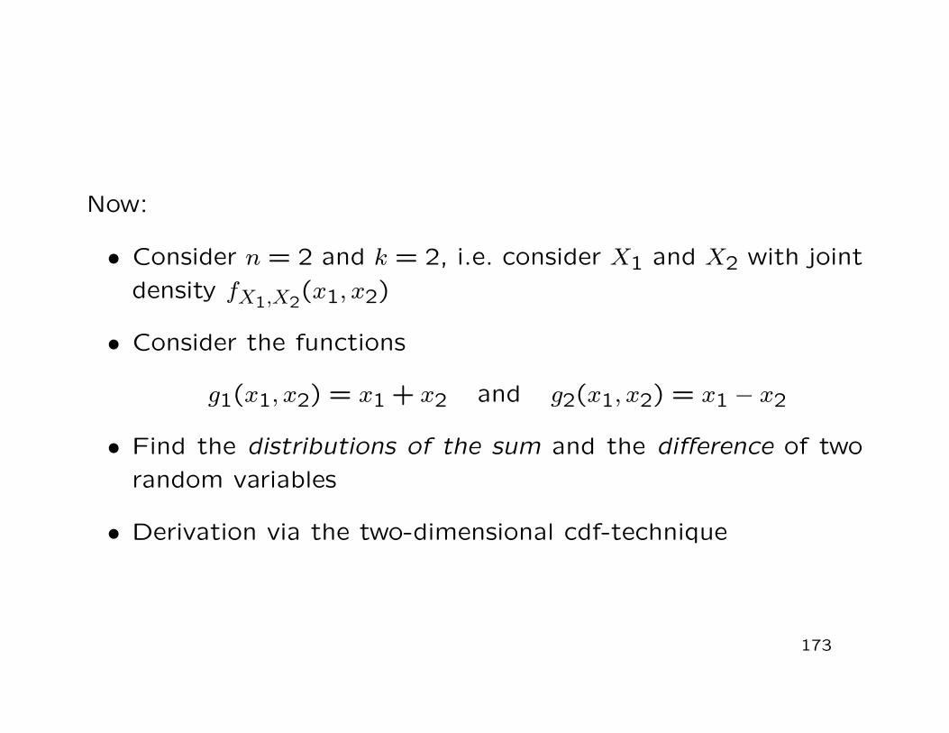
Now:

• Consider n = 2 and k = 2, i.e. consider X1 and X2 with jointdensity fX1,X2(x1, x2)

• Consider the functions

g1(x1, x2) = x1 + x2 and g2(x1, x2) = x1 − x2

• Find the distributions of the sum and the difference of tworandom variables

• Derivation via the two-dimensional cdf-technique

173

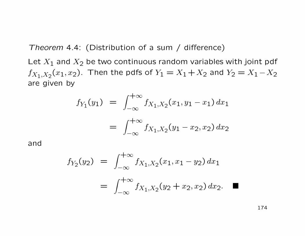
Theorem 4.4: (Distribution of a sum / difference)

Let X1 and X2 be two continuous random variables with joint pdffX1,X2(x1, x2). Then the pdfs of Y1 = X1+X2 and Y2 = X1−X2are given by

fY1(y1) =∫ +∞

−∞fX1,X2(x1, y1 − x1) dx1

=∫ +∞

−∞fX1,X2(y1 − x2, x2) dx2

and

fY2(y2) =∫ +∞

−∞fX1,X2(x1, x1 − y2) dx1

=∫ +∞

−∞fX1,X2(y2 + x2, x2) dx2.

174

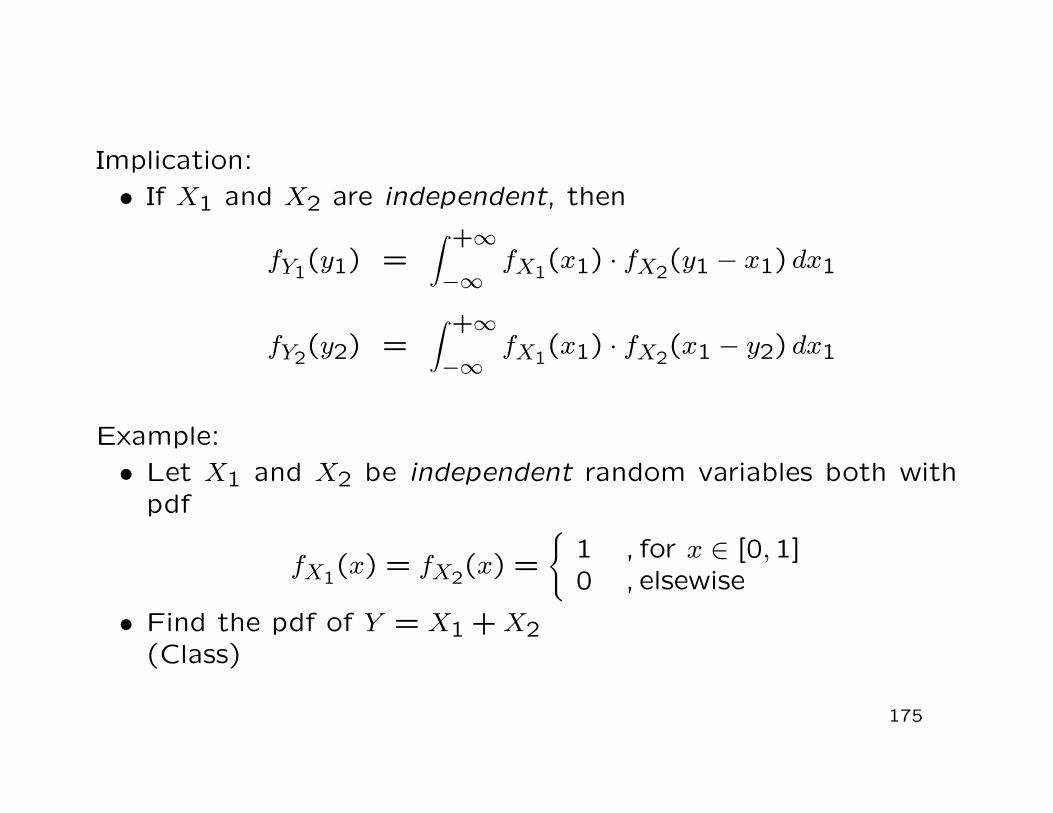
Implication:• If X1 and X2 are independent, then

fY1(y1) =∫ +∞

−∞fX1(x1) · fX2(y1 − x1) dx1

fY2(y2) =∫ +∞

−∞fX1(x1) · fX2(x1 − y2) dx1

Example:• Let X1 and X2 be independent random variables both with

pdf

fX1(x) = fX2(x) =

1 , for x ∈ [0,1]0 , elsewise

• Find the pdf of Y = X1 + X2(Class)

175

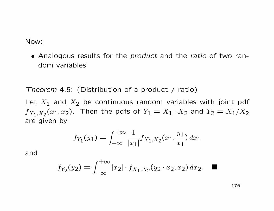
Now:

• Analogous results for the product and the ratio of two ran-dom variables

Theorem 4.5: (Distribution of a product / ratio)

Let X1 and X2 be continuous random variables with joint pdffX1,X2(x1, x2). Then the pdfs of Y1 = X1 ·X2 and Y2 = X1/X2are given by

fY1(y1) =∫ +∞

−∞

1|x1|

fX1,X2(x1,y1

x1) dx1

and

fY2(y2) =∫ +∞

−∞|x2| · fX1,X2(y2 · x2, x2) dx2.

176

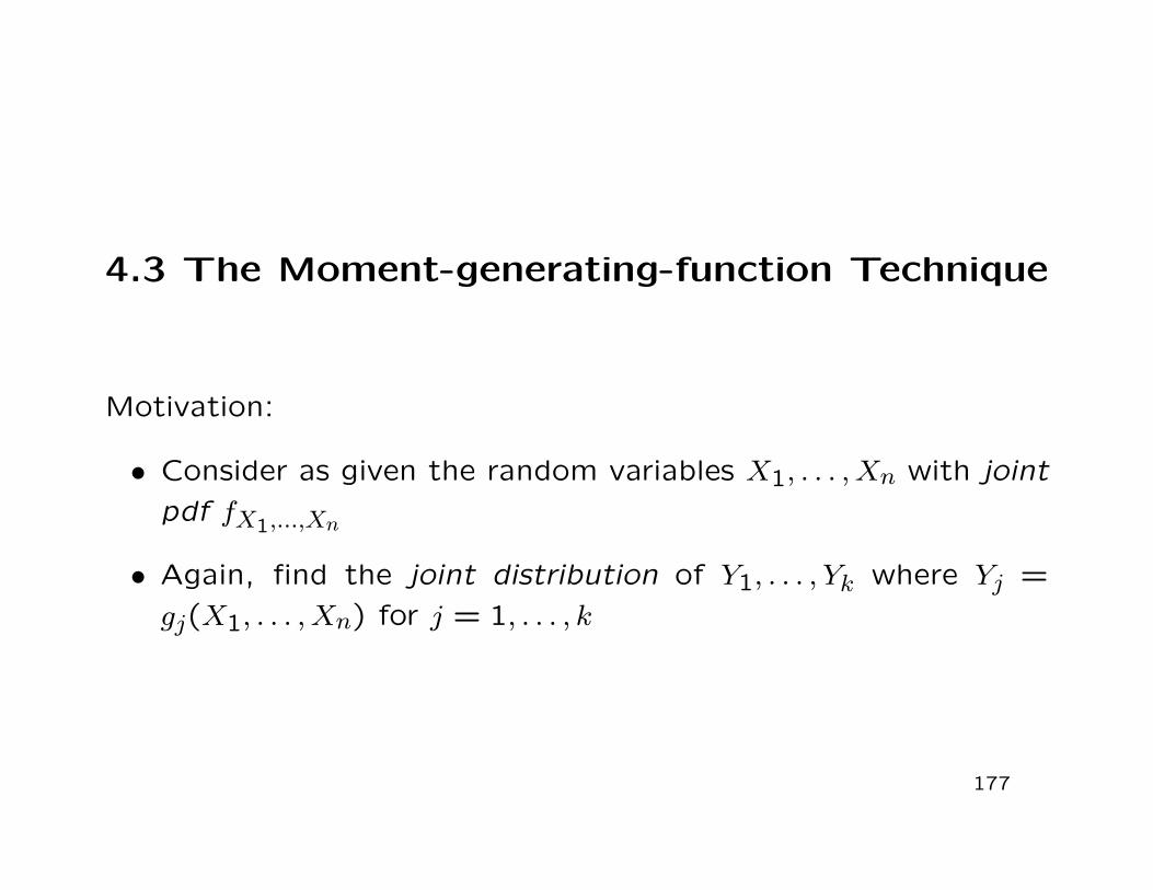
4.3 The Moment-generating-function Technique

Motivation:

• Consider as given the random variables X1, . . . , Xn with jointpdf fX1,...,Xn

• Again, find the joint distribution of Y1, . . . , Yk where Yj =gj(X1, . . . , Xn) for j = 1, . . . , k

177

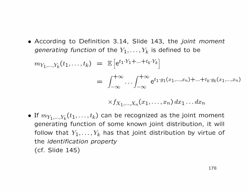
• According to Definition 3.14, Slide 143, the joint momentgenerating function of the Y1, . . . , Yk is defined to be

mY1,...,Yk(t1, . . . , tk) = E

[

et1·Y1+...+tk·Yk]

=∫ +∞

−∞. . .

∫ +∞

−∞et1·g1(x1,...,xn)+...+tk·gk(x1,...,xn)

×fX1,...,Xn(x1, . . . , xn) dx1 . . . dxn

• If mY1,...,Yk(t1, . . . , tk) can be recognized as the joint moment

generating function of some known joint distribution, it willfollow that Y1, . . . , Yk has that joint distribution by virtue ofthe identification property(cf. Slide 145)

178

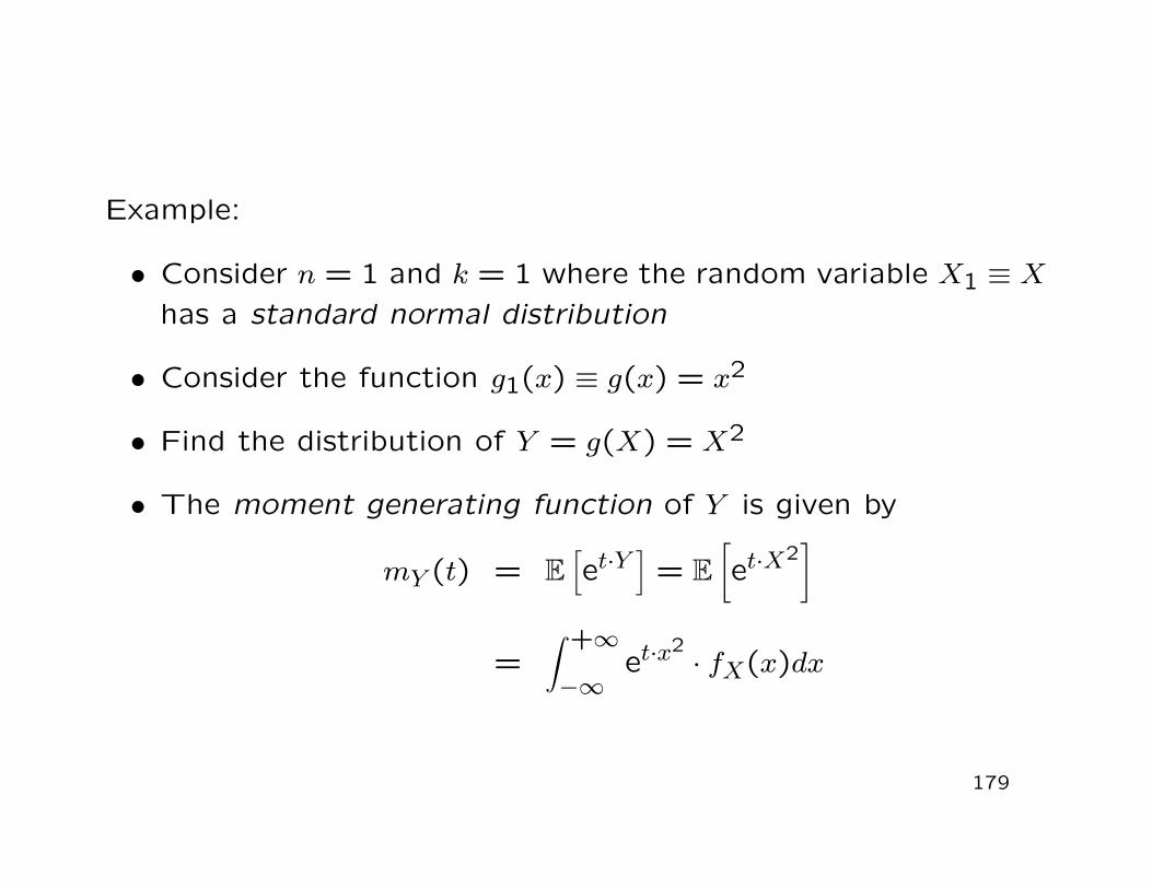
Example:

• Consider n = 1 and k = 1 where the random variable X1 ≡ Xhas a standard normal distribution

• Consider the function g1(x) ≡ g(x) = x2

• Find the distribution of Y = g(X) = X2

• The moment generating function of Y is given by

mY (t) = E[

et·Y]

= E[

et·X2]

=∫ +∞

−∞et·x2

· fX(x)dx

179

=∫ +∞

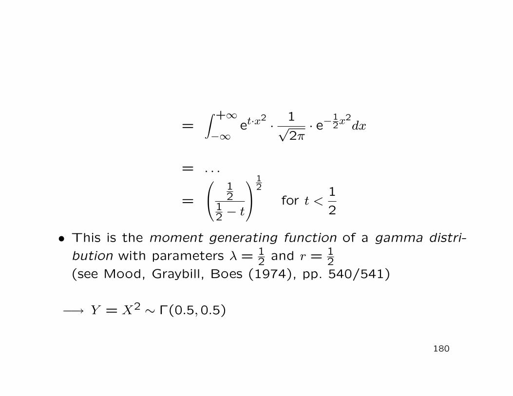
−∞et·x2

·1√2π

· e−12x2

dx

= . . .

=

12

12 − t

12

for t <12

• This is the moment generating function of a gamma distri-bution with parameters λ = 1

2 and r = 12

(see Mood, Graybill, Boes (1974), pp. 540/541)

−→ Y = X2 ∼ Γ(0.5,0.5)

180

Now:

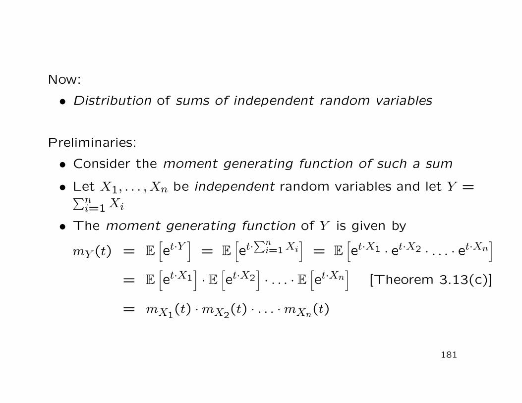
• Distribution of sums of independent random variables

Preliminaries:

• Consider the moment generating function of such a sum

• Let X1, . . . , Xn be independent random variables and let Y =∑n

i=1 Xi

• The moment generating function of Y is given by

mY (t) = E[

et·Y]

= E[

et·∑n

i=1 Xi]

= E[

et·X1 · et·X2 · . . . · et·Xn]

= E[

et·X1]

· E[

et·X2]

· . . . · E[

et·Xn]

[Theorem 3.13(c)]

= mX1(t) ·mX2(t) · . . . ·mXn(t)

181

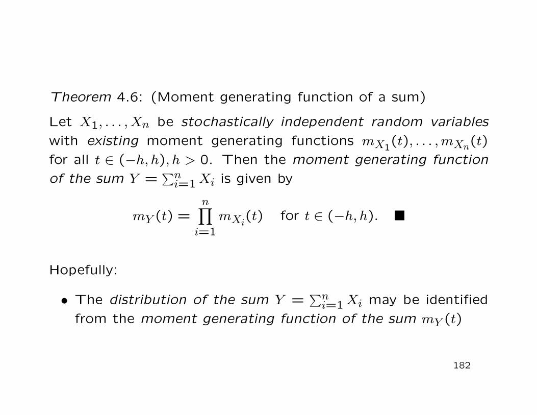
Theorem 4.6: (Moment generating function of a sum)

Let X1, . . . , Xn be stochastically independent random variableswith existing moment generating functions mX1(t), . . . , mXn(t)for all t ∈ (−h, h), h > 0. Then the moment generating functionof the sum Y =

∑ni=1 Xi is given by

mY (t) =n∏

i=1mXi(t) for t ∈ (−h, h).

Hopefully:

• The distribution of the sum Y =∑n

i=1 Xi may be identifiedfrom the moment generating function of the sum mY (t)

182

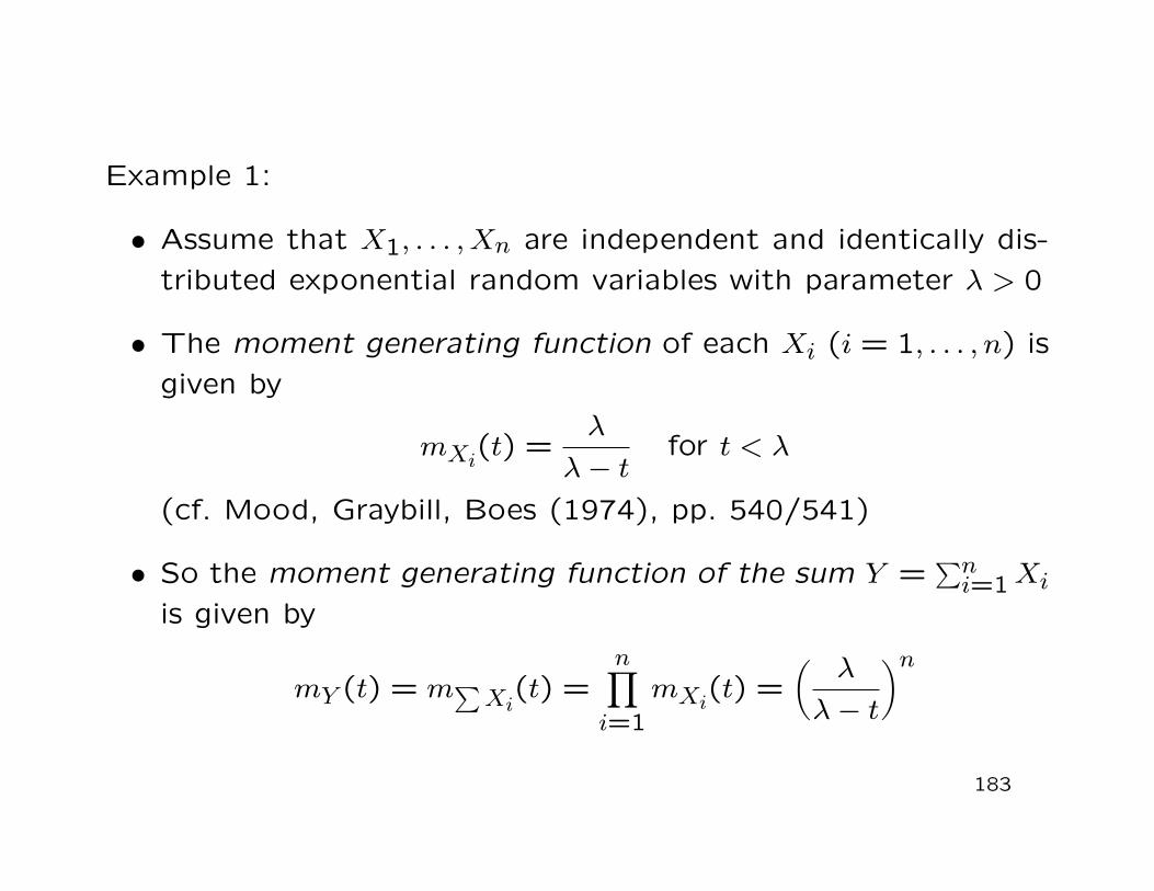
Example 1:

• Assume that X1, . . . , Xn are independent and identically dis-tributed exponential random variables with parameter λ > 0

• The moment generating function of each Xi (i = 1, . . . , n) isgiven by

mXi(t) =λ

λ− tfor t < λ

(cf. Mood, Graybill, Boes (1974), pp. 540/541)

• So the moment generating function of the sum Y =∑n

i=1 Xiis given by

mY (t) = m∑

Xi(t) =

n∏

i=1mXi(t) =

( λλ− t

)n

183

• This is the moment generating function of a Γ(n, λ) distri-bution(cf. Mood, Graybill, Boes (1974), pp. 540/541)

−→ the sum of n independent, identically distributed expo-nential random variables with parameter λ has a Γ(n, λ)distribution

184

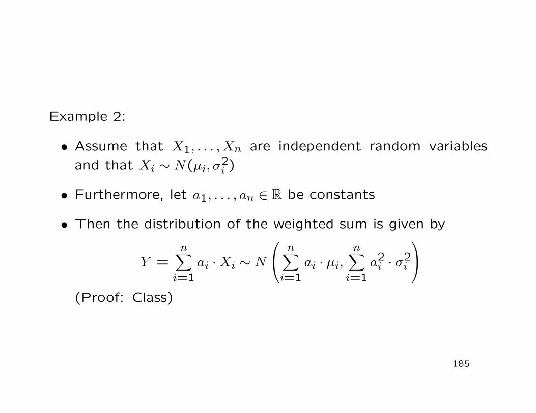
Example 2:

• Assume that X1, . . . , Xn are independent random variablesand that Xi ∼ N(µi, σ2

i )

• Furthermore, let a1, . . . , an ∈ R be constants

• Then the distribution of the weighted sum is given by

Y =n

∑

i=1ai ·Xi ∼ N

n∑

i=1ai · µi,

n∑

i=1a2

i · σ2i

(Proof: Class)

185

4.4 General Transformations

Up to now:

• Techniques that allow us, under special circumstances, tofind the distributions of the transformed variables

Y1 = g1(X1, . . . , Xn), . . . , Yk = gk(X1, . . . , Xn)

However:

• These methods do not necessarily hit the mark(e.g. if calculations get too complicated)

186

Resort:

• There are constructive methods by which it is generally pos-sible (under rather mild conditions) to find the distributionsof transformed random variables−→ transformation theorems

Here:

• We restrict attention to the simplest case where n = 1, k = 1,i.e. we consider the transformation Y = g(X)

• For multivariate extensions (i.e. for n ≥ 1, k ≥ 1) see Mood,Graybill, Boes (1974), pp. 203-212

187

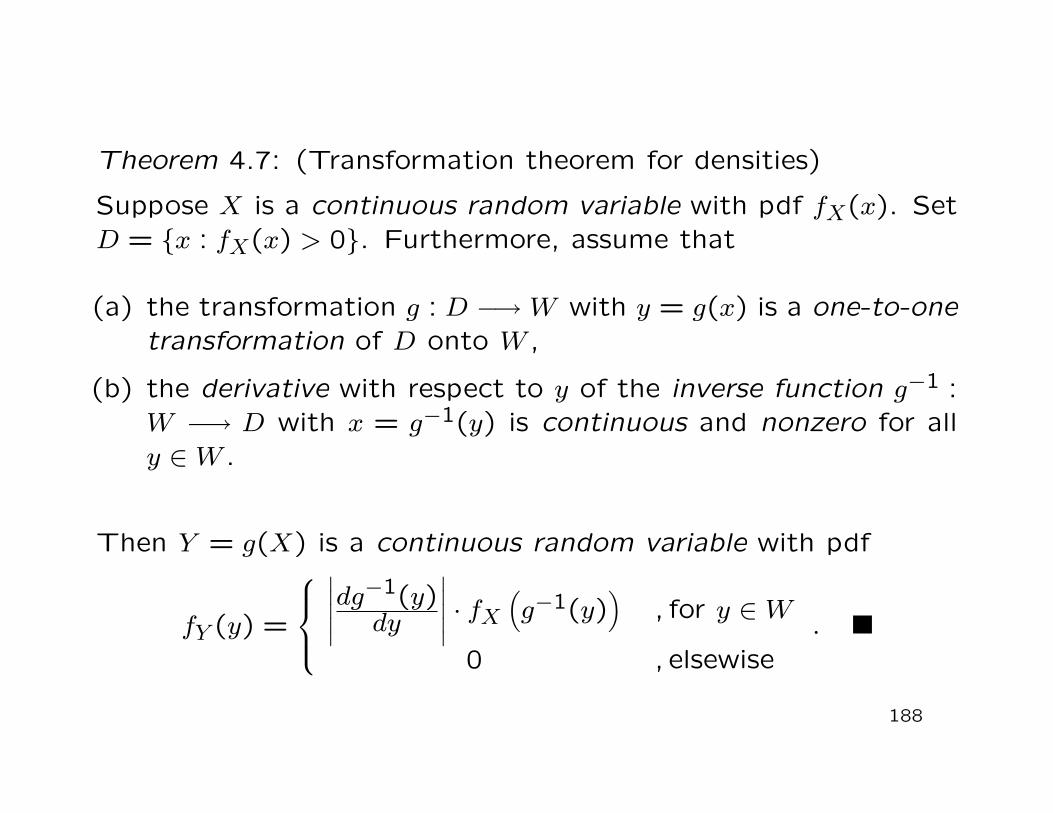
Theorem 4.7: (Transformation theorem for densities)

Suppose X is a continuous random variable with pdf fX(x). SetD = x : fX(x) > 0. Furthermore, assume that

(a) the transformation g : D −→ W with y = g(x) is a one-to-onetransformation of D onto W ,

(b) the derivative with respect to y of the inverse function g−1 :W −→ D with x = g−1(y) is continuous and nonzero for ally ∈ W .

Then Y = g(X) is a continuous random variable with pdf

fY (y) =

∣

∣

∣

∣

∣

dg−1(y)dy

∣

∣

∣

∣

∣

· fX(

g−1(y))

, for y ∈ W

0 , elsewise.

188

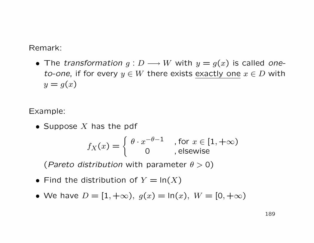
Remark:

• The transformation g : D −→ W with y = g(x) is called one-to-one, if for every y ∈ W there exists exactly one x ∈ D withy = g(x)

Example:

• Suppose X has the pdf

fX(x) =

θ · x−θ−1 , for x ∈ [1,+∞)0 , elsewise

(Pareto distribution with parameter θ > 0)

• Find the distribution of Y = ln(X)

• We have D = [1,+∞), g(x) = ln(x), W = [0,+∞)

189

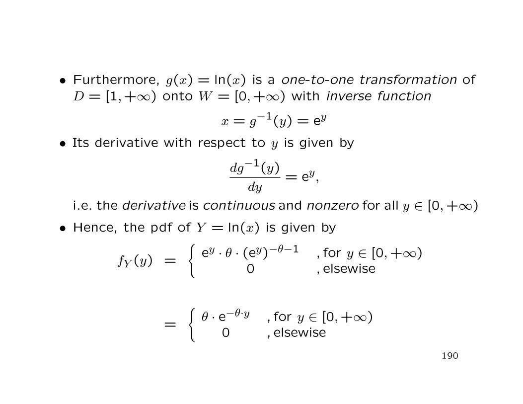
• Furthermore, g(x) = ln(x) is a one-to-one transformation ofD = [1,+∞) onto W = [0,+∞) with inverse function

x = g−1(y) = ey

• Its derivative with respect to y is given by

dg−1(y)dy

= ey,

i.e. the derivative is continuous and nonzero for all y ∈ [0,+∞)

• Hence, the pdf of Y = ln(x) is given by

fY (y) =

ey · θ · (ey)−θ−1 , for y ∈ [0,+∞)0 , elsewise

=

θ · e−θ·y , for y ∈ [0,+∞)0 , elsewise

190

5. Methods of Estimation

Setting:

• Let X be a random variable (or let X be a random vector)representing a random experiment

• We are interested in the actual distribution of X (or X)

Notice:

• In practice the actual distribution of X is a priori unknown

191

Therefore:

• Collect information on the unknown distribution by repeat-edly observing the random experiment (and thus the randomvariable X)

−→ random sample−→ statistic−→ estimator

192

5.1 Sampling, Estimators, Limit Theorems

Setting:

• Let X represent the random experiment under consideration(X is a univariate random variable)

• We intend to observe the random experiment (i.e. X) n times

• Prior to the explicit realizations we may consider the potentialobservations as a set of n random variables X1, . . . , Xn

193

Definition 5.1: (Random sample)

The random variables X1, . . . , Xn are defined to be a randomsample from X if

(a) each Xi, i = 1, . . . , n, has the same distribution as X,

(b) X1, . . . , Xn are stochastically independent.

The number n is called the sample size.

194

Remarks:

• We assume that, in principle, the random experiment can berepeated as often as desired

• We call the realizations x1, . . . , xn of the random sampleX1, . . . , Xn the observed or the concrete sample

• Considering the random sample X1, . . . , Xn as a random vec-tor, we see that its joint density is given by

fX1,...,Xn(x1, . . . , xn) =n∏

i=1fXi(xi)

(since the Xi’s are independent; cf. Definition 3.8, Slide 125)

195

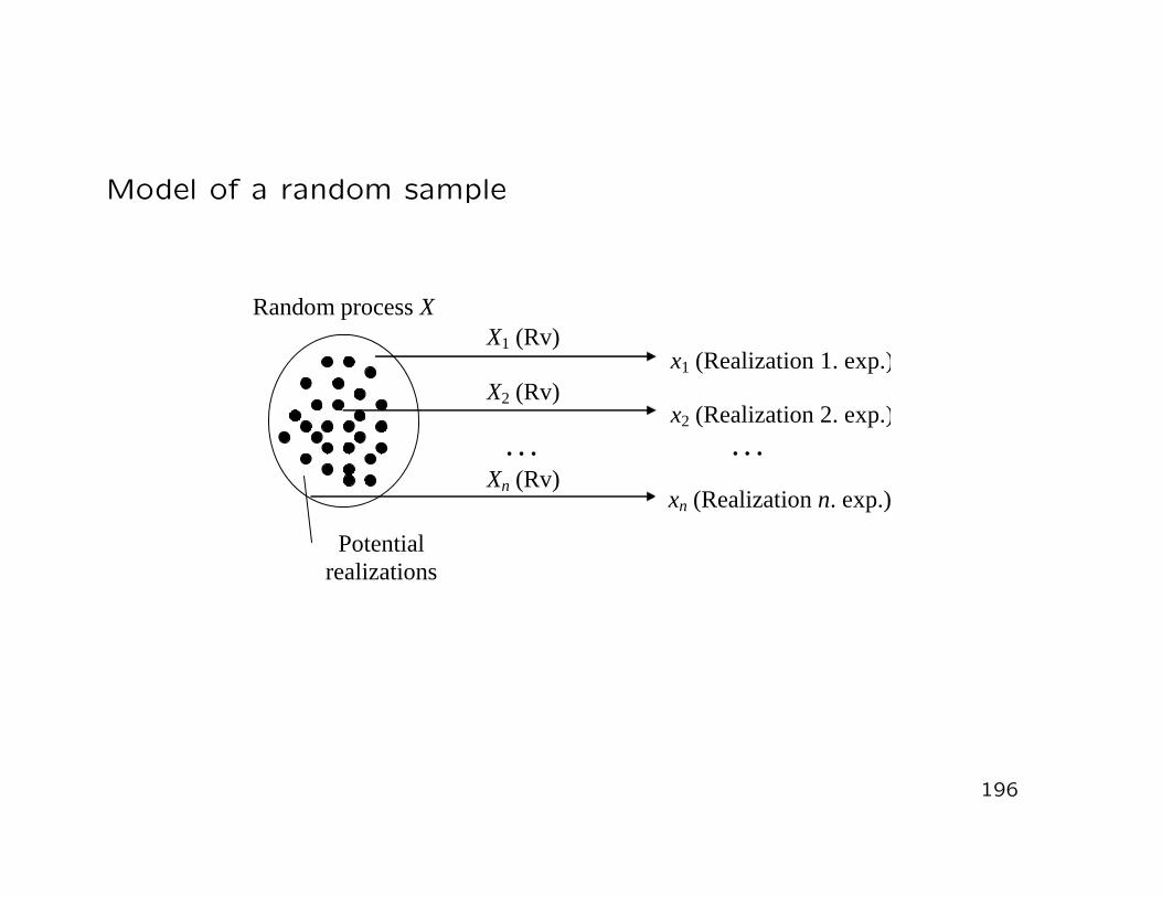
Model of a random sample

196

Random process X

Potential realizations

X1 (Rv) x1 (Realization 1. exp.)

X2 (Rv)

Xn (Rv)

x2 (Realization 2. exp.)

xn (Realization n. exp.)

. . . . . .

Now:

• Consider functions of the sampling variables X1, . . . , Xn

−→ statistic−→ estimator

Definition 5.2: (Statistic)

Let X1, . . . , Xn be a random sample from X and let g : Rn −→ Rbe a real-valued function with n arguments that does not containany unknown parameters. Then the random variable

T = g(X1, . . . , Xn)

is called a statistic.

197

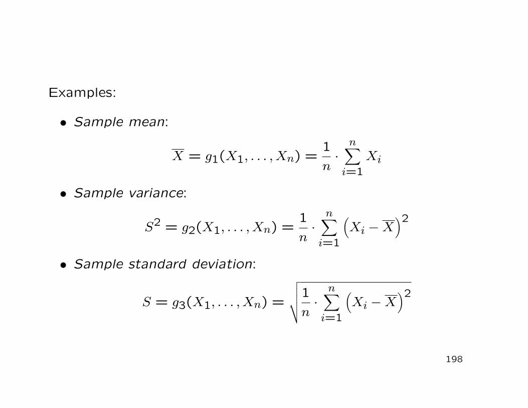
Examples:

• Sample mean:

X = g1(X1, . . . , Xn) =1n·

n∑

i=1Xi

• Sample variance:

S2 = g2(X1, . . . , Xn) =1n·

n∑

i=1

(

Xi −X)2

• Sample standard deviation:

S = g3(X1, . . . , Xn) =

√

√

√

√

1n·

n∑

i=1

(

Xi −X)2

198

Remarks:

• All these concepts can be extended to the multivariate case

• The statistic T = g(X1, . . . , Xn) is a function of random vari-ables and hence it is itself a random variable−→ a statistic has a distribution

(and, in particular, an expectation and a variance)

Purposes of statistics:

• Statistics provide information on the distribution of X

• Statistics are central tools forestimating parametershypothesis-testing on parameters

199

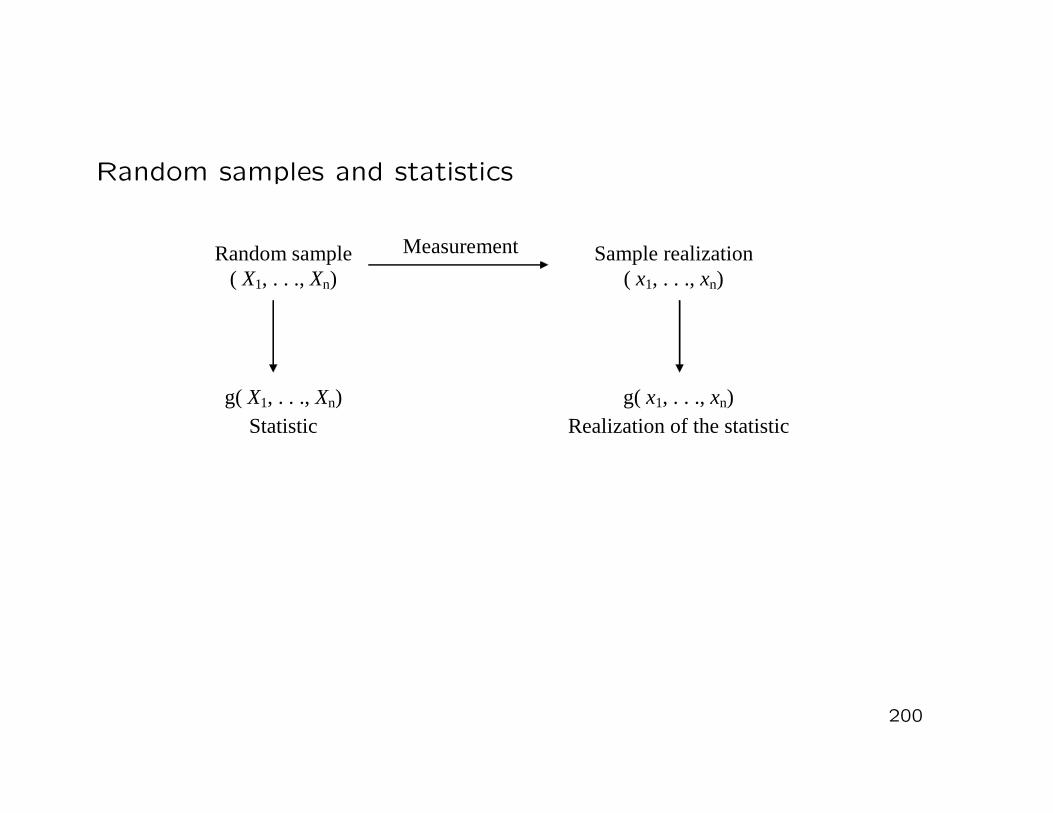
Random samples and statistics

200

Random sample

( X1, . . ., Xn) Measurement Sample realization

( x1, . . ., xn)

g( X1, . . ., Xn) Statistic

g( x1, . . ., xn) Realization of the statistic

Now:

• Let X be a random variable with unknown cdf FX(x)

• We may be interested in one or several unknown parametersof X

• Let θ denote this unknown vector of parameters, e.g.

θ =

[

E(X)Var(X)

]

• Frequently, the distribution family of X is known, e.g. X ∼N(µ, σ2), but we do not know the specific parameters. Then

θ =

[

µσ2

]

• We will estimate the unknown parameter vector on the basisof statistics from a random sample X1, . . . , Xn

201

Definition 5.3: (Estimator, estimate)

The statistic θ(X1, . . . , Xn) is called estimator (or point estima-tor) of the unknown parameter vector θ. After having observedthe concrete sample x1, . . . , xn, we call the realization of the es-timator θ(x1, . . . , xn) an estimate.

Remarks:

• The estimator θ(X1, . . . , Xn) is a random variable or a randomvector−→ an estimator has a (joint) distribution, an expected value

(or vector) and a variance (or a covariance matrix)

• The estimate θ(x1, . . . , xn) is a number (or a vector of num-bers)

202

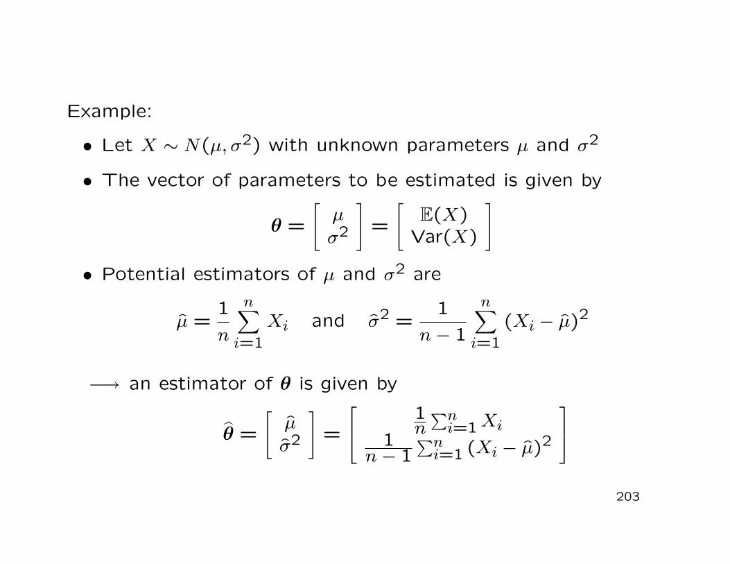
Example:

• Let X ∼ N(µ, σ2) with unknown parameters µ and σ2

• The vector of parameters to be estimated is given by

θ =

[

µσ2

]

=

[

E(X)Var(X)

]

• Potential estimators of µ and σ2 are

µ =1n

n∑

i=1Xi and σ2 =

1n− 1

n∑

i=1(Xi − µ)2

−→ an estimator of θ is given by

θ =

[

µσ2

]

=

1n

∑ni=1 Xi

1n− 1

∑ni=1 (Xi − µ)2

203

Question:

• Why do we need this seemingly complicated concept of anestimator in the form of a random variable?

Answer:

• To establish a comparison between alternative estimators ofthe parameter vector θ

Example:

• Let θ = Var(X) denote the unknown variance of X

204

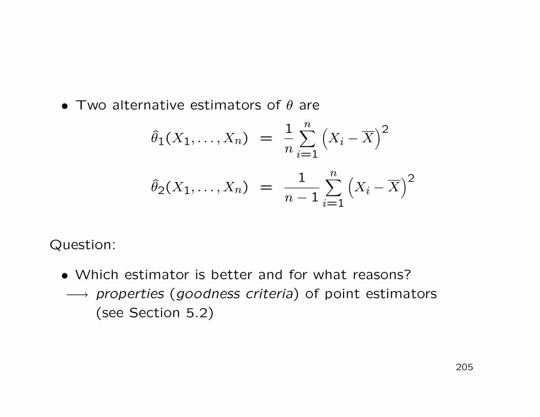
• Two alternative estimators of θ are

θ1(X1, . . . , Xn) =1n

n∑

i=1

(

Xi −X)2

θ2(X1, . . . , Xn) =1

n− 1

n∑

i=1

(

Xi −X)2

Question:

• Which estimator is better and for what reasons?−→ properties (goodness criteria) of point estimators

(see Section 5.2)

205

Notice:

• Some of these criteria qualify estimators in terms of theirproperties when the sample size becomes large(n →∞, large-sample-properties)

Therefore:

• Explanation of the concept of stochastic convergence:

Central-limit theorem

Weak law of large numbers

Convergence in probability

Convergence in distribution

206

Theorem 5.4: (Univariate central-limit theorem)

Let X be any arbitrary random variable with E(X) = µ andVar(X) = σ2. Let X1, . . . , Xn be a random sample from X andlet

Xn =1n

n∑

i=1Xi

denote the arithmetic sample mean. Then, for n →∞, we have

Xn ∼ N

(

µ,σ2

n

)

and√

nXn − µ

σ∼ N(0,1).

Next:

• Generalization to the multivariate case

207

Theorem 5.5: (Multivariate central-limit theorem)

Let X = (X1, . . . , Xm)′ be any arbitrary random vector withE(X) = µ and Cov(X) = Σ. Let X1, . . . ,Xn be a (multivari-ate) random sample from X and let

Xn =1n

n∑

i=1Xi

denote the multivariate arithmetic sample mean. Then, for n →∞, we have

Xn ∼ N(

µ,1nΣ

)

and√

n(

Xn − µ)

∼ N(0,Σ).

208

Remarks:

• A multivariate random sample from the random vector Xarises naturally by replacing all univariate random variablesin Definition 5.1 (Slide 194) by corresponding multivariaterandom vectors

• Note the formal analogy to the univariate case in Theorem5.4(be aware of matrix-calculus rules!)

Next:

• Famous theorem on the arithmetic sample mean

209

Theorem 5.6: (Weak law of large numbers)

Let X1, X2, . . . be a sequence of independent and identically dis-tributed random variables with

E(Xi) = µ < ∞,

Var(Xi) = σ2 < ∞.

Consider the random variable

Xn =1n

n∑

i=1Xi

(arithmetic sample mean). Then, for any ε > 0 we have

limn→∞P

(∣

∣

∣Xn − µ∣

∣

∣ ≥ ε)

= 0.

210

Remarks:

• Theorem 5.6 is known as the weak law of large numbers

• Irrespective of how small we choose ε > 0, the probabilitythat Xn deviates more than ±ε from its expectation µ tendsto zero when the sample size increases

• Notice the analogy between a sequence of independent andidentically distributed random variables and the definition ofa random sample from X on Slide 194

Next:

• The first important concept of limiting behaviour

211

Definition 5.7: (Convergence in probability)

Let Y1, Y2, . . . be a sequence of random variables. We say thatthe sequence Y1, Y2, . . . converges in probability to θ, if for anyε > 0 we have

limn→∞P (|Yn − θ| ≥ ε) = 0.

We denote convergence in probability by

plim Yn = θ or Ynp→ θ.

Remarks:

• Specific case: Weak law of large numbers

plim Xn = µ or Xnp→ µ

212

• Typically (but not necessarily) a sequence of random vari-ables converges in probability to a constant θ ∈ R

• For multivariate sequences of random vectors Y1,Y2, . . . theDefinition 5.7 has to be applied to the respective correspond-ing elements

• The concept of convergence in probability is important toqualifying estimators

Next:

• Alternative concepts of stochastic convergence

213

Definition 5.8: (Convergence in distribution)

Let Y1, Y2, . . . be a sequence of random variables and let Z also bea random variable. We say that the sequence Y1, Y2, . . . convergesin distribution to the distribution of Z if

limn→∞FYn(y) = FZ(y) for any y ∈ R.

We denote convergence in distribution by

Ynd→ Z.

Remarks:• Specific case: central-limit theorem

Yn =√

nXn − µ

σd→ U ∼ N(0,1)

• In the case of convergence in distribution, the sequence ofrv’s always converges to a limiting random variable

214

Theorem 5.9: (Rules for probability limits)

Let X1, X2, . . . and Y1, Y2, . . . be sequences of random variableswith plim Xn = a and plim Yn = b. Then

(a) plim (Xn ± Yn) = a± b,

(b) plim (Xn · Yn) = a · b,

(c) plim(Xn

Yn

)

= ab (for b 6= 0).

(d) (Slutsky-Theorem) If g : R −→ R is a continuous function ina ∈ R, then

plim g (Xn) = g(a).

215

Remark:

• There is a property similar to Slutsky’s theorem that holdsfor the convergence in distribution

Theorem 5.10: (Rule for limiting distributions)

Let X1, X2, . . . be a sequence of random variables and let Z be a

random variable such that Xnd→ Z. If h : R −→ R is a continuous

function, then

h (Xn)d→ h(Z).

Next:

• Connection of both convergence concepts

216

Theorem 5.11: (Cramer-Theorem)

Let X1, X2, . . . and Y1, Y2, . . . be sequences of random variables,let Z be a random variable and a ∈ R a constant. Assume thatplim Xn = a and Yn

d→ Z. Then

(a) Xn + Ynd→ a + Z,

(b) Xn · Ynd→ a · Z.

Example:

• Let X1, . . . , Xn be a random sample from X with E(X) = µand Var(X) = σ2

217

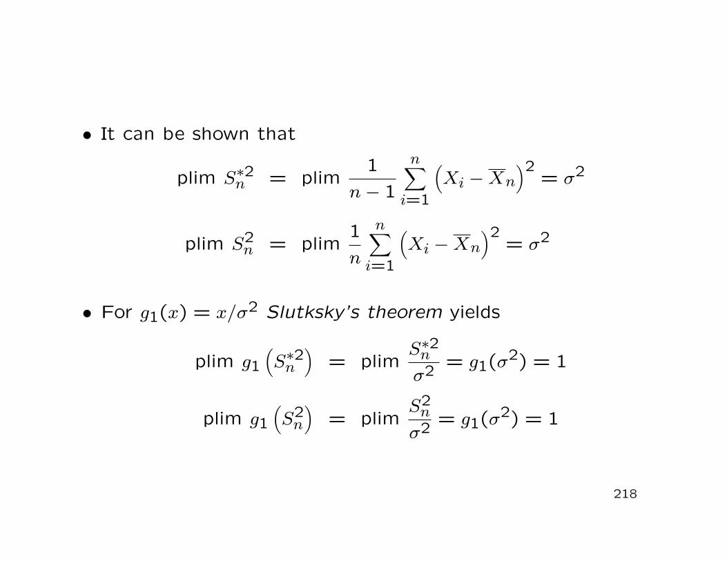
• It can be shown that

plim S∗2n = plim1

n− 1

n∑

i=1

(

Xi −Xn)2

= σ2

plim S2n = plim

1n

n∑

i=1

(

Xi −Xn)2

= σ2

• For g1(x) = x/σ2 Slutksky’s theorem yields

plim g1(

S∗2n)

= plimS∗2nσ2 = g1(σ

2) = 1

plim g1(

S2n

)

= plimS2

nσ2 = g1(σ

2) = 1

218

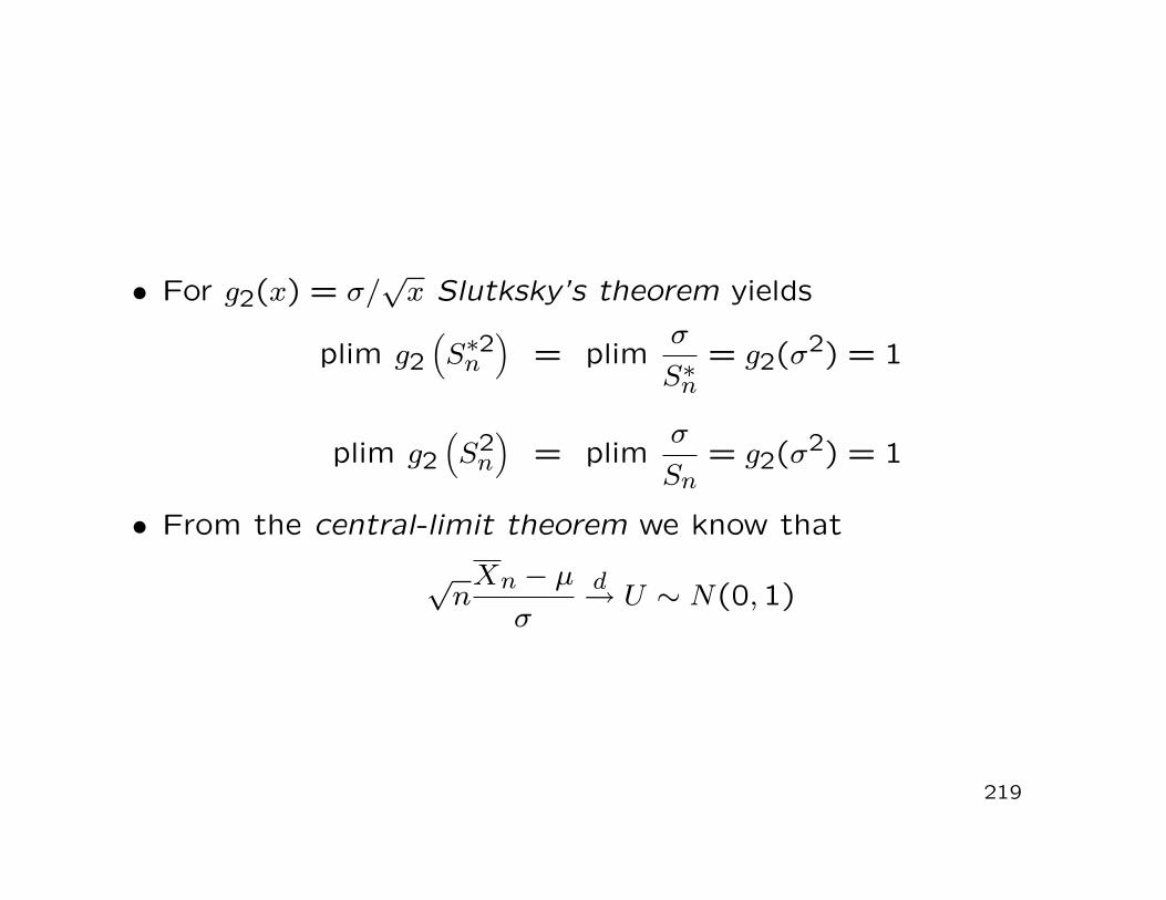
• For g2(x) = σ/√

x Slutksky’s theorem yields

plim g2(

S∗2n)

= plimσS∗n

= g2(σ2) = 1

plim g2(

S2n

)

= plimσSn

= g2(σ2) = 1

• From the central-limit theorem we know that

√n

Xn − µσ

d→ U ∼ N(0,1)

219

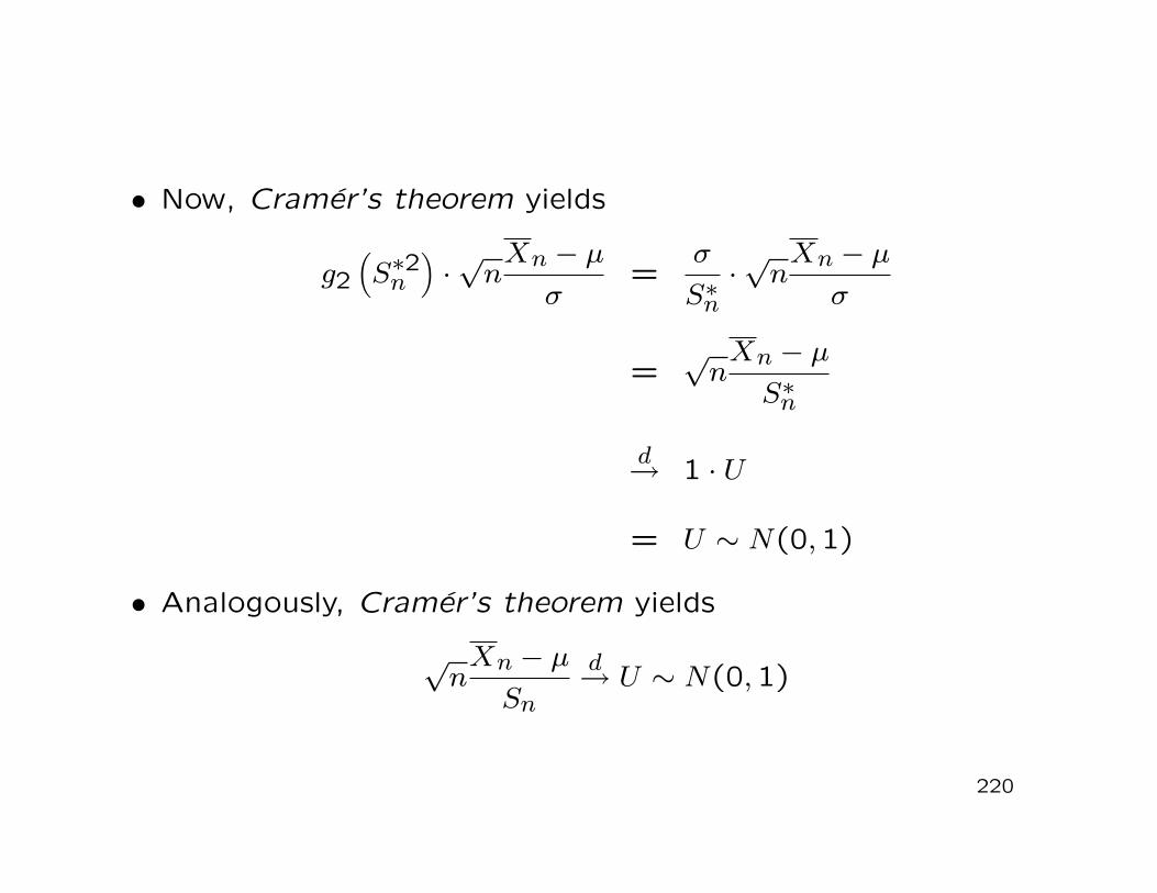
• Now, Cramer’s theorem yields

g2(

S∗2n)

·√

nXn − µ

σ=

σS∗n

·√

nXn − µ

σ

=√

nXn − µ

S∗n

d→ 1 · U

= U ∼ N(0,1)

• Analogously, Cramer’s theorem yields

√n

Xn − µSn

d→ U ∼ N(0,1)

220

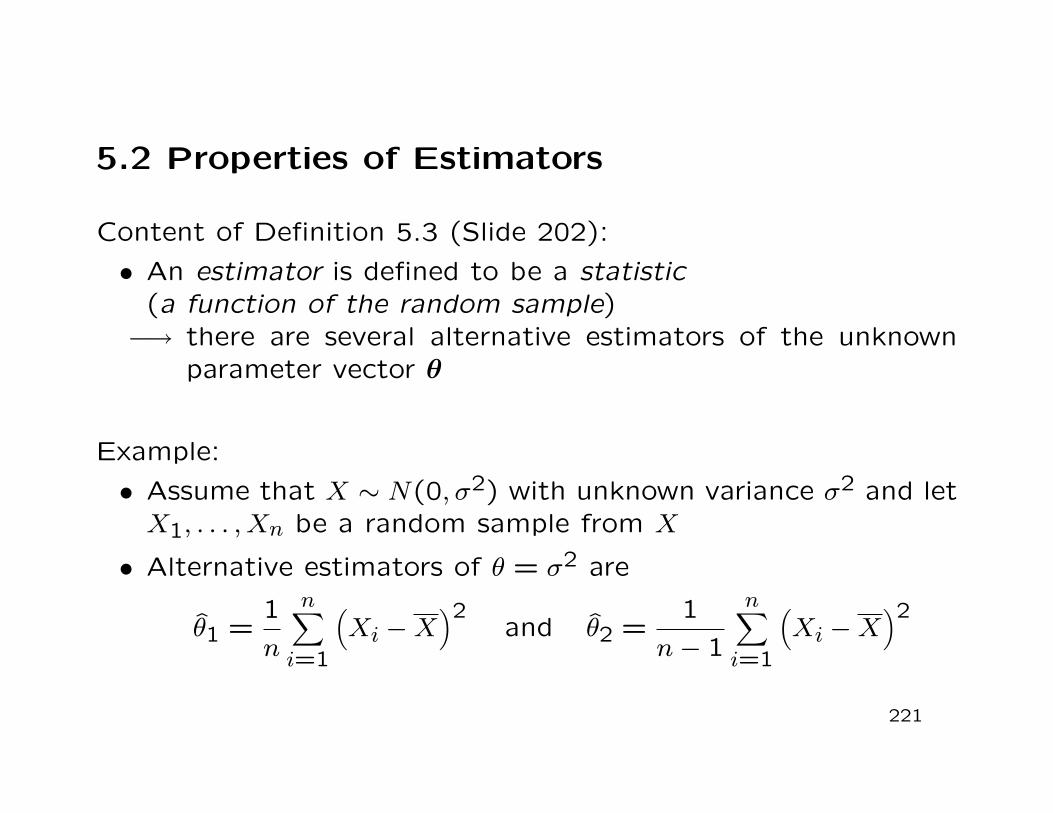
5.2 Properties of Estimators

Content of Definition 5.3 (Slide 202):

• An estimator is defined to be a statistic(a function of the random sample)−→ there are several alternative estimators of the unknown

parameter vector θ

Example:

• Assume that X ∼ N(0, σ2) with unknown variance σ2 and letX1, . . . , Xn be a random sample from X

• Alternative estimators of θ = σ2 are

θ1 =1n

n∑

i=1

(

Xi −X)2

and θ2 =1

n− 1

n∑

i=1

(

Xi −X)2

221

Important questions:

• Are there reasonable criteria according to which we can selecta ’good’ estimator?

• How can we construct ’good’ estimators?

First goodness property of point estimators:

• Concept of repeated sampling:Draw several random samples from XConsider the estimator for each random sampleAn ’average’ of the estimates should be ’close’ to theunknown parameter(no systematic bias)

−→ unbiasedness of an estimator

222

Definition 5.12: (Unbiasedness, bias)

An estimator θ(X1, . . . , Xn) of the unknown parameter θ is definedto be an unbiased estimator if its expectation coincides with theparameter to be estimated, i.e. if

E[

θ(X1, . . . , Xn)]

= θ.

The bias of the estimator is defined as

Bias(θ) = E(θ)− θ.

Remarks:

• Definition 5.12 easily generalizes to the multivariate case

• The bias of an unbiased estimator is equal to zero

223

Now:• Important and very general result

Theorem 5.13: (Unbiased estimators of E(X) and Var(X))

Let X1, . . . , Xn be a random sample form X where X may bearbitrarily distributed with unknown expectation µ = E(X) andunknown variance σ2 = Var(X). Then the estimators

µ(X1, . . . , Xn) = X =1n·

n∑

i=1Xi

and

σ2(X1, . . . , Xn) = S2 =1

n− 1·

n∑

i=1

(

Xi −X)2

are always unbiased estimators of the parameters µ = E(X) andσ2 = Var(X), respectively.

224

Remarks:

• Proof: Class

• Note that no explicit distribution of X is required

• Unbiasedness does, in general, not carry over to parametertransformations. For example,

S =√

S2 is not a unbiased estimator of σ = SD(X) =√

Var(X)

Question:

• How can we compare two alternative unbiased estimators ofthe parameter θ?

225

Definition 5.14: (Relative efficiency)

Let θ1 and θ2 be two unbiased estimators of the unknown pa-rameter θ. θ1 is defined to be relatively more efficient than θ2if

Var(θ1) ≤ Var(θ2)

for all possible parameter values of θ and

Var(θ1) < Var(θ2)

for at least one possible parameter value of θ.

226

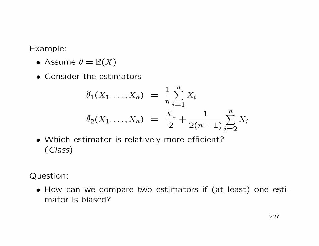
Example:

• Assume θ = E(X)

• Consider the estimators

θ1(X1, . . . , Xn) =1n

n∑

i=1Xi

θ2(X1, . . . , Xn) =X1

2+

12(n− 1)

n∑

i=2Xi

• Which estimator is relatively more efficient?(Class)

Question:

• How can we compare two estimators if (at least) one esti-mator is biased?

227

Definition 5.15: (Mean-squared error)

Let θ be an estimator of the parameter θ. The mean-squarederror of the estimator θ is defined to be

MSE(θ) = E[

(

θ − θ)2

]

= Var(

θ)

+[

Bias(θ)]2

.

Remarks:

• If an estimator is unbiased, then its MSE is equal to thevariance of the estimator

• The MSE of an estimator θ depends on the value of theunknown parameter θ

228

Next:

• Comparison of alternative estimators via their MSE’s

Definition 5.16: (MSE efficiency)

Let θ1 and θ2 be two alternative estimators of the unknownparameter θ. θ1 is defined to be more MSE efficient than θ2 if

MSE(θ1) ≤ MSE(θ2)

for all possible parameter values of θ and

MSE(θ1) < MSE(θ2)

for at least one possible parameter value of θ.

229

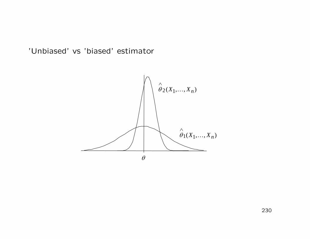
’Unbiased’ vs ’biased’ estimator

230

),,( 12 nXX K∧θ

),,( 11 nXX K∧θ

θ

Remarks:

• Frequently 2 estimators of θ are not comparable with respectto MSE efficiency since their respective MSE curves cross

• There is no general mathematical principle for constructingMSE efficient estimators

• However, there are methods for finding the estimator withuniformly minimum-variance among all unbiased estimators−→ restriction to the class of all unbiased estimators

• These specific methods are not discussed here(Rao-Blackwell-Theorem, Lehmann-Scheffe-Theorem)

• Here, we consider only one important result

231

Theorem 5.17: (Cramer-Rao lower bound for variance)

Let X1, . . . , Xn be a random sample from X and let θ be a param-eter to be estimated. Consider the joint density of the randomsample fX1,...,Xn(x1, . . . , xn) and define the value

CR(θ) ≡

E

(

∂ fX1,...,Xn(X1, . . . , Xn)

∂ θ

)2

−1

.

Under certain (regularity) conditions we have for any unbiasedestimator θ(X1, . . . , Xn)

Var(θ) ≥ CR(θ).

232

Remarks:

• The value CR(θ) is the minimal variance that any unbiasedestimator can take on

−→ goodness criterion for unbiased estimators

• If for an unbiased estimator θ(X1, . . . , Xn)

Var(θ) = CR(θ),

then θ is called UMVUE(Uniformly Minimum-Variance Unbiased Estimator)

233

Second goodness property of point estimators:

• Consider an increasing sample size (n →∞)

Notation: θn(X1, . . . , Xn) = θ(X1, . . . , Xn)

Analysis of the asymptotic distribution properties of θn

−→ consistency of an estimator

Definition 5.18: ((Weak) consistency)

The estimator θn(X1, . . . , Xn) is called (weakly) consistent for θif it converges in probability to θ, i.e. if

plim θn(X1, . . . , Xn) = θ.

234

Example:

• Assume that X ∼ N(µ, σ2) with known σ2 (e.g. σ2 = 1)

• Consider the following two estimators of µ:

µn(X1, . . . , Xn) =1n

n∑

i=1Xi

µ∗n(X1, . . . , Xn) =1n

n∑

i=1Xi +

2n

• µn is (weakly) consistent for µ(Theorem 5.6, Slide 210: weak law of large numbers)

235

• µ∗n is (weakly) consistent for µ(this follows from Theorem 5.9(a), Slide 215)

• Exact distribution of µn:

µn ∼ N(µ, σ2/n)

(linear transformation of the normal distribution)

• Exact distribution of µ∗n:

µ∗n ∼ N(µ + 2/n, σ2/n)

(linear transformation of the normal distribution)

236

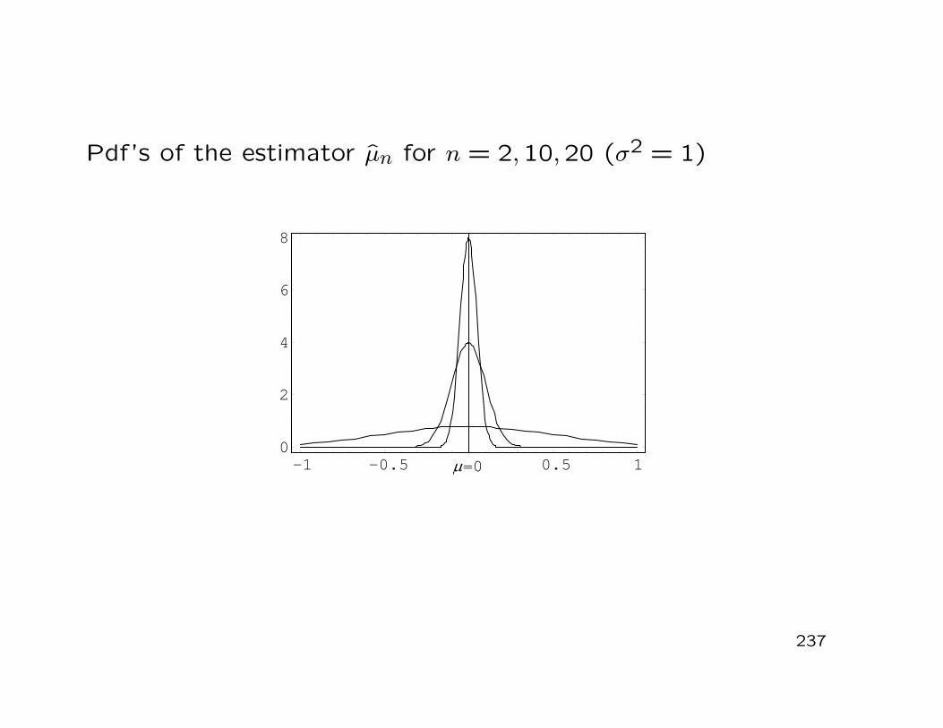
Pdf’s of the estimator µn for n = 2,10,20 (σ2 = 1)

237

6

4

2

-1 -0.5 µ=0 0.5 1 0

8

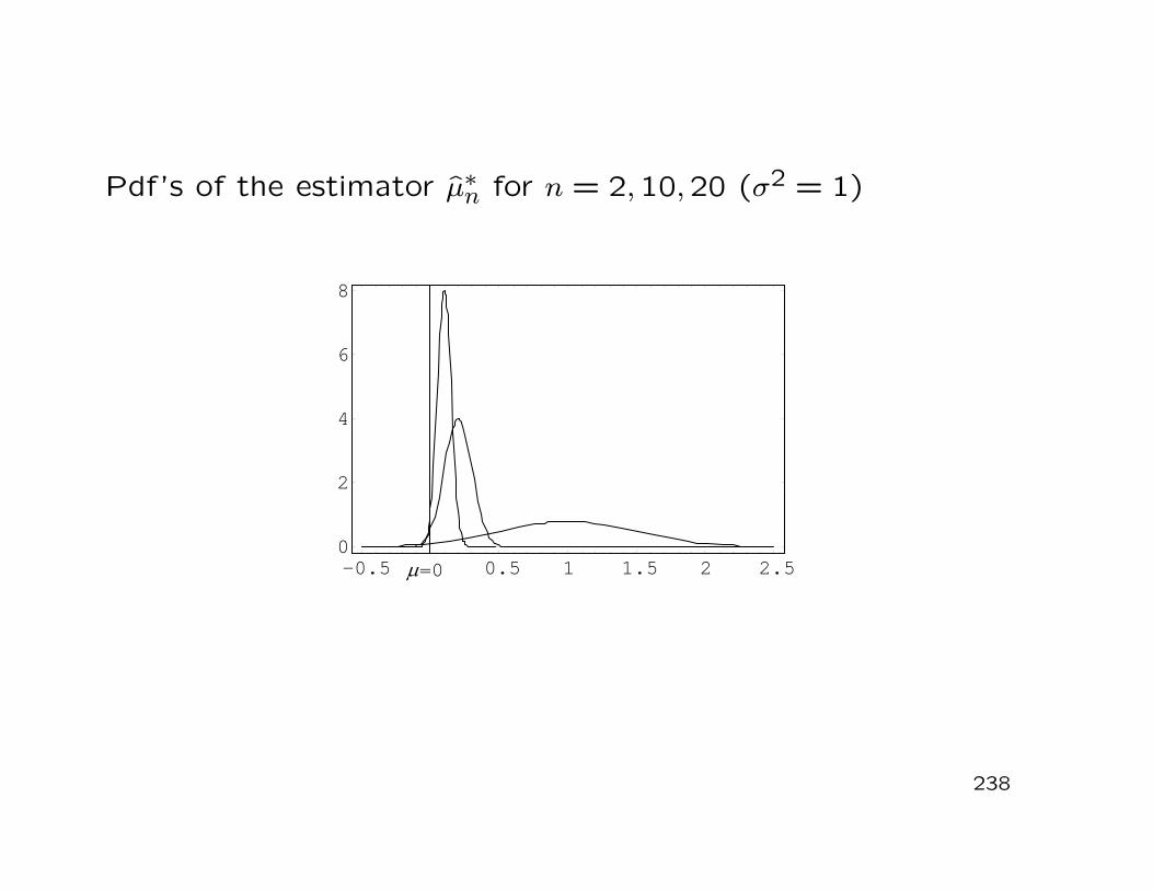
Pdf’s of the estimator µ∗n for n = 2,10,20 (σ2 = 1)

238

6

4

2

-0.5 µ=0 0.5 1 1.5 2 2.5 0

8

Remarks:

• Sufficient (but not necessary) condition for consistency:

limn→∞E(θn) = θ (asymptotic unbiasedness)

limn→∞Var(θn) = 0

• Possible properties of an estimator:

consistent and unbiased

inconsistent and unbiased

consistent and biased

inconsistent and biased

239

Next:

• Application of the central-limit theorem to estimators

−→ asymptotic normality of an estimator

Definition 5.19: (Asymptotic normality)

An estimator θn(X1, . . . , Xn) of the parameter θ is called asymp-totically normal if there exist (1) a sequence of real constantsθ1, θ2, . . . and (2) a function V (θ) such that

√n ·

(

θn − θn) d→ U ∼ N(0, V (θ)).

240

Remarks:

• Alternative notation:

θnappr.∼ N(θn, V (θ)/n)

• The concept of asymptotic normality naturally extends tomultivariate settings

241

5.3 Methods of Estimation

Up to now:

• Definitions + properties of estimators

Next:

• Construction of estimators

Three classical methods:

• Method of Lesst Squares (LS)

• Method of Moments (MM)

• Maximum-Likelihood method (ML)

242

Remarks:

• There are further methods(e.g. the Generalized Method-of-Moments, GMM)

• Here: focus on ML estimation

243

5.3.1 Least-Squares Estimators

History:• Introduced by

A.M. Legendre (1752-1833)C.F. Gauß (1777-1855)

Idee:• Approximate the (noisy) observations x1, . . . , xn by functions

gi(θ1, . . . , θm), i = 1, . . . , n, m < n such that

S(x1, . . . , xn; θ) =n

∑

i=1[xi − gi(θ)]2 −→ min

θ• The LS-estimator is then defined to be

θ(X1, . . . , Xn) = argmin S(X1, . . . , Xn; θ)

244

Remark:

• The LS-method is central to the linear regression model(cf. the courses ’Econometrics’ I + II)

245

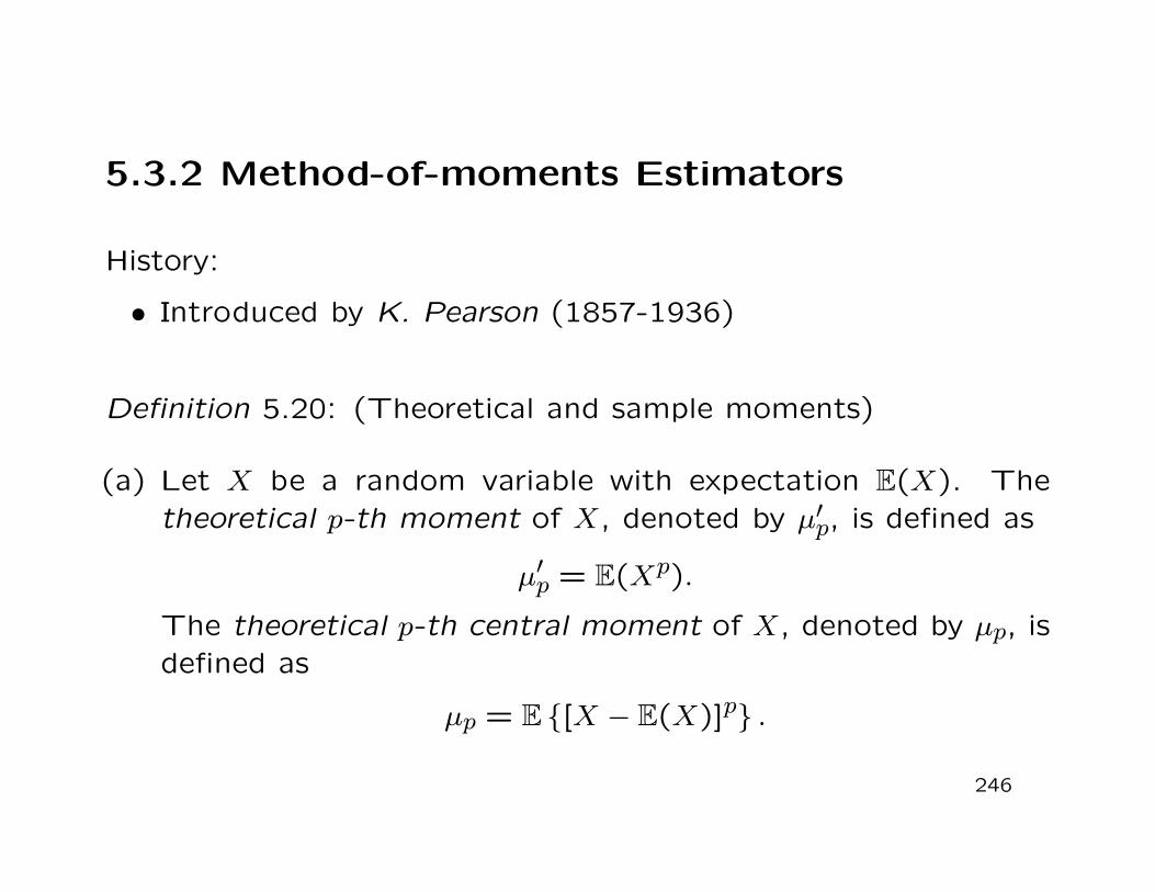
5.3.2 Method-of-moments Estimators

History:

• Introduced by K. Pearson (1857-1936)

Definition 5.20: (Theoretical and sample moments)

(a) Let X be a random variable with expectation E(X). Thetheoretical p-th moment of X, denoted by µ′p, is defined as

µ′p = E(Xp).

The theoretical p-th central moment of X, denoted by µp, isdefined as

µp = E [X − E(X)]p .

246

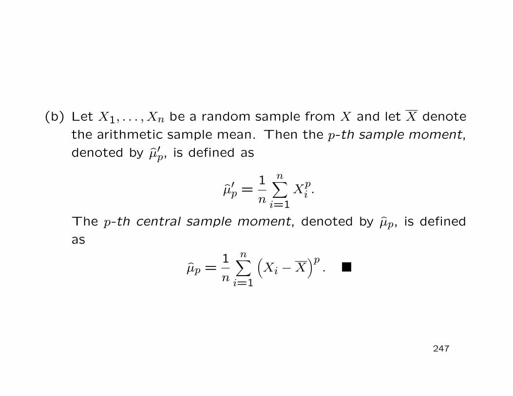
(b) Let X1, . . . , Xn be a random sample from X and let X denotethe arithmetic sample mean. Then the p-th sample moment,denoted by µ′p, is defined as

µ′p =1n

n∑

i=1Xp

i .

The p-th central sample moment, denoted by µp, is definedas

µp =1n

n∑

i=1

(

Xi −X)p

.

247

Remarks:

• The theoretical moments µ′p and µp had already been intro-duced in Definition 2.21 (Slide 76)

• The sample moments µ′p and µp are (weakly) consistent es-timators of the theoretical moments µ′p and µp

• The arithmetic sample mean is the 1st sample moment ofX1, . . . , Xn

• The sample variance is the 2nd central sample moment ofX1, . . . , Xn

248

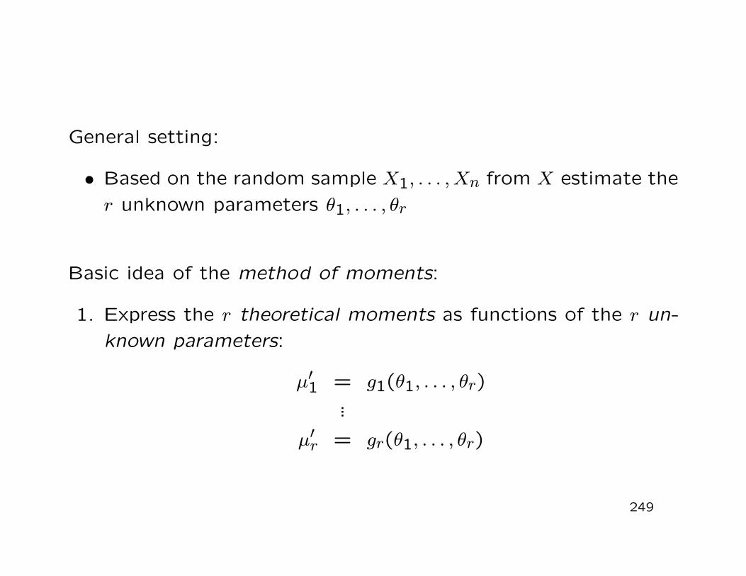
General setting:

• Based on the random sample X1, . . . , Xn from X estimate ther unknown parameters θ1, . . . , θr

Basic idea of the method of moments:

1. Express the r theoretical moments as functions of the r un-known parameters:

µ′1 = g1(θ1, . . . , θr)...

µ′r = gr(θ1, . . . , θr)

249

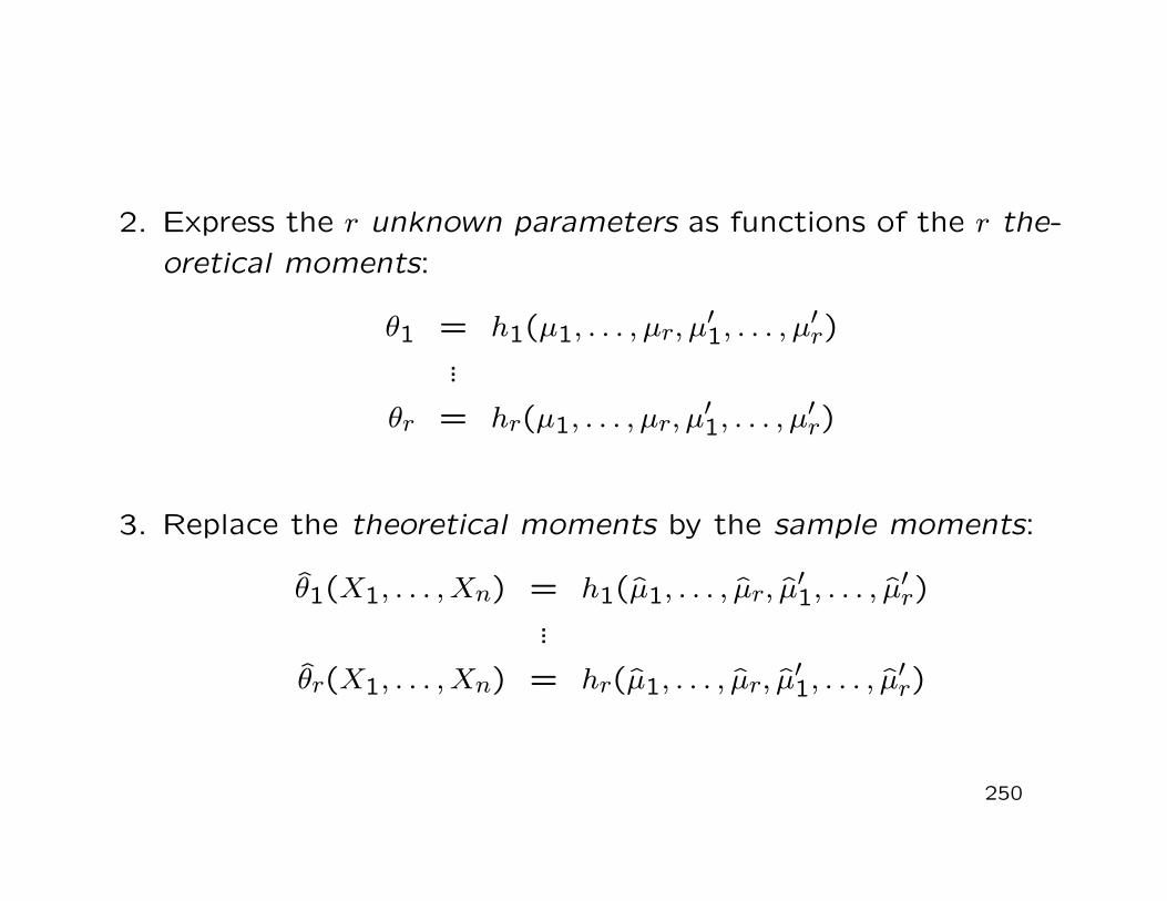
2. Express the r unknown parameters as functions of the r the-oretical moments:

θ1 = h1(µ1, . . . , µr, µ′1, . . . , µ′r)...

θr = hr(µ1, . . . , µr, µ′1, . . . , µ′r)

3. Replace the theoretical moments by the sample moments:

θ1(X1, . . . , Xn) = h1(µ1, . . . , µr, µ′1, . . . , µ′r)...

θr(X1, . . . , Xn) = hr(µ1, . . . , µr, µ′1, . . . , µ′r)

250

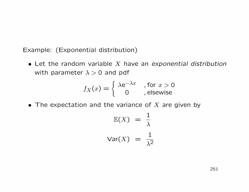
Example: (Exponential distribution)

• Let the random variable X have an exponential distributionwith parameter λ > 0 and pdf

fX(x) =

λe−λx , for x > 00 , elsewise

• The expectation and the variance of X are given by

E(X) =1λ

Var(X) =1λ2

251

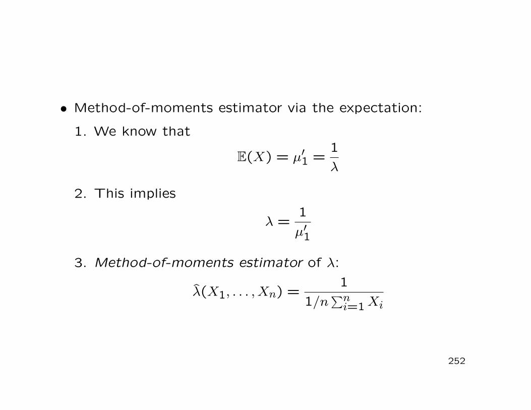
• Method-of-moments estimator via the expectation:

1. We know that

E(X) = µ′1 =1λ

2. This implies

λ =1µ′1

3. Method-of-moments estimator of λ:

λ(X1, . . . , Xn) =1

1/n∑n

i=1 Xi

252

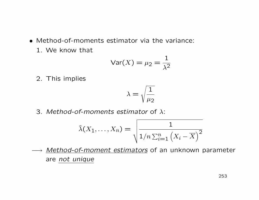
• Method-of-moments estimator via the variance:

1. We know that

Var(X) = µ2 =1λ2

2. This implies

λ =

√

1µ2

3. Method-of-moments estimator of λ:

λ(X1, . . . , Xn) =

√

√

√

√

√

1

1/n∑n

i=1

(

Xi −X)2

−→ Method-of-moment estimators of an unknown parameterare not unique

253

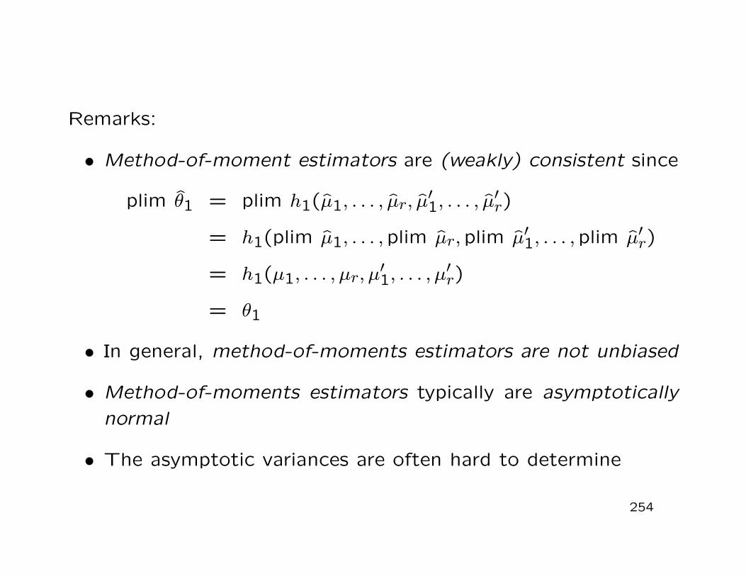
Remarks:

• Method-of-moment estimators are (weakly) consistent since

plim θ1 = plim h1(µ1, . . . , µr, µ′1, . . . , µ′r)

= h1(plim µ1, . . . ,plim µr,plim µ′1, . . . ,plim µ′r)

= h1(µ1, . . . , µr, µ′1, . . . , µ′r)

= θ1

• In general, method-of-moments estimators are not unbiased

• Method-of-moments estimators typically are asymptoticallynormal

• The asymptotic variances are often hard to determine

254

5.3.3 Maximum-Likelihood Estimators

History:

• Introduced by Ronald Fisher (1890-1962)

Basic idea behind ML estimation:

• We estimate the unknown parameters θ1, . . . , θr in such amanner that the likelihood of the observed sample x1, . . . , xn,which we express as a function of the unknown parameters,becomes maximal

255

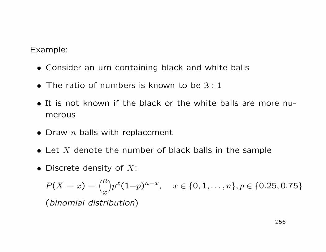
Example:

• Consider an urn containing black and white balls

• The ratio of numbers is known to be 3 : 1

• It is not known if the black or the white balls are more nu-merous

• Draw n balls with replacement

• Let X denote the number of black balls in the sample

• Discrete density of X:

P (X = x) =(nx

)

px(1−p)n−x, x ∈ 0,1, . . . , n, p ∈ 0.25,0.75

(binomial distribution)

256

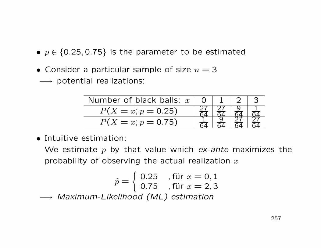
• p ∈ 0.25,0.75 is the parameter to be estimated

• Consider a particular sample of size n = 3−→ potential realizations:

Number of black balls: x 0 1 2 3P (X = x; p = 0.25) 27

642764

964

164

P (X = x; p = 0.75) 164

964

2764

2764

• Intuitive estimation:We estimate p by that value which ex-ante maximizes theprobability of observing the actual realization x

p =

0.25 , fur x = 0,10.75 , fur x = 2,3

−→ Maximum-Likelihood (ML) estimation

257

Next:

• Formalization of the ML estimation technique

Notions:

• Likelihood-, Loglikelihood function

• ML estimator

Definition 5.21: (Likelihood function)

The likelihood function of n random variables X1, . . . , Xn is de-fined to be the joint density of the n random variables, sayfX1,...,Xn(x1, . . . , xn; θ), which is considered to be a function ofthe parameter vector θ.

258

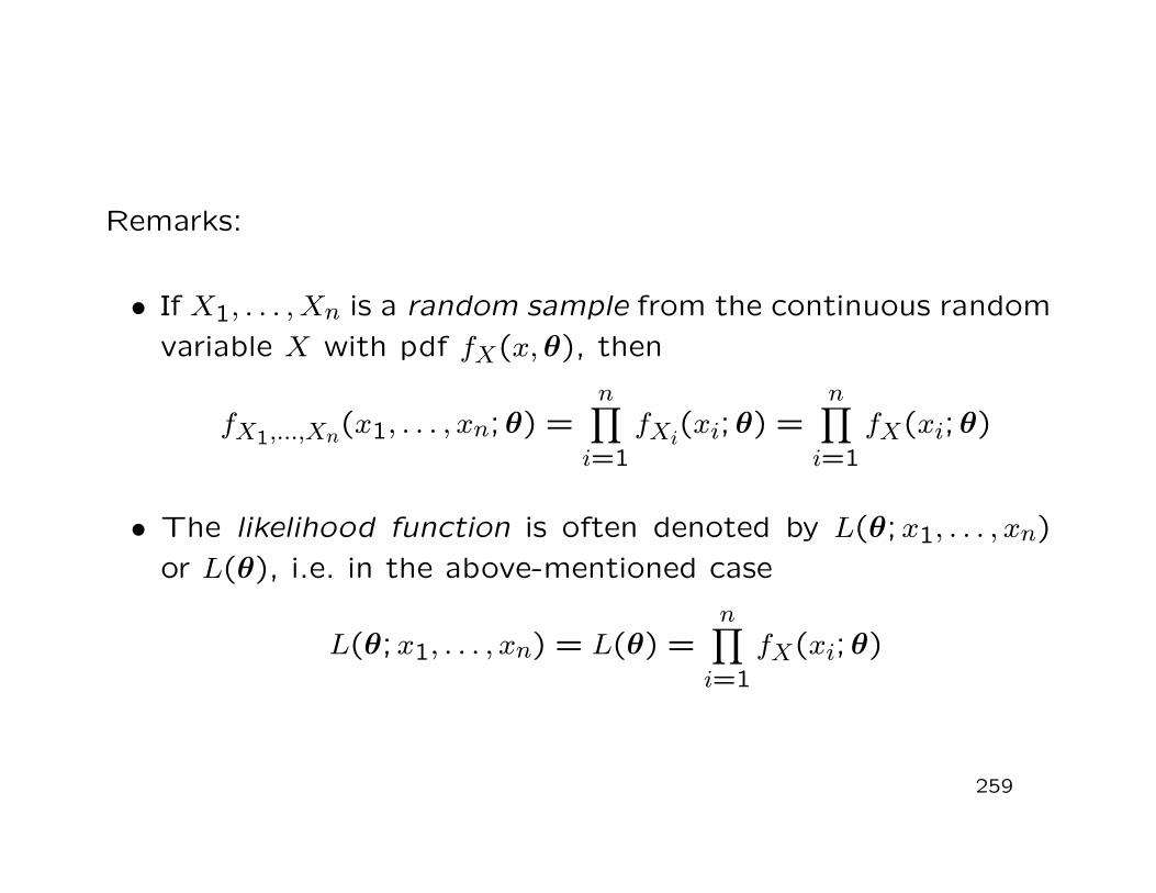
Remarks:

• If X1, . . . , Xn is a random sample from the continuous randomvariable X with pdf fX(x, θ), then

fX1,...,Xn(x1, . . . , xn; θ) =n∏

i=1fXi(xi; θ) =

n∏

i=1fX(xi; θ)

• The likelihood function is often denoted by L(θ;x1, . . . , xn)or L(θ), i.e. in the above-mentioned case

L(θ;x1, . . . , xn) = L(θ) =n∏

i=1fX(xi; θ)

259

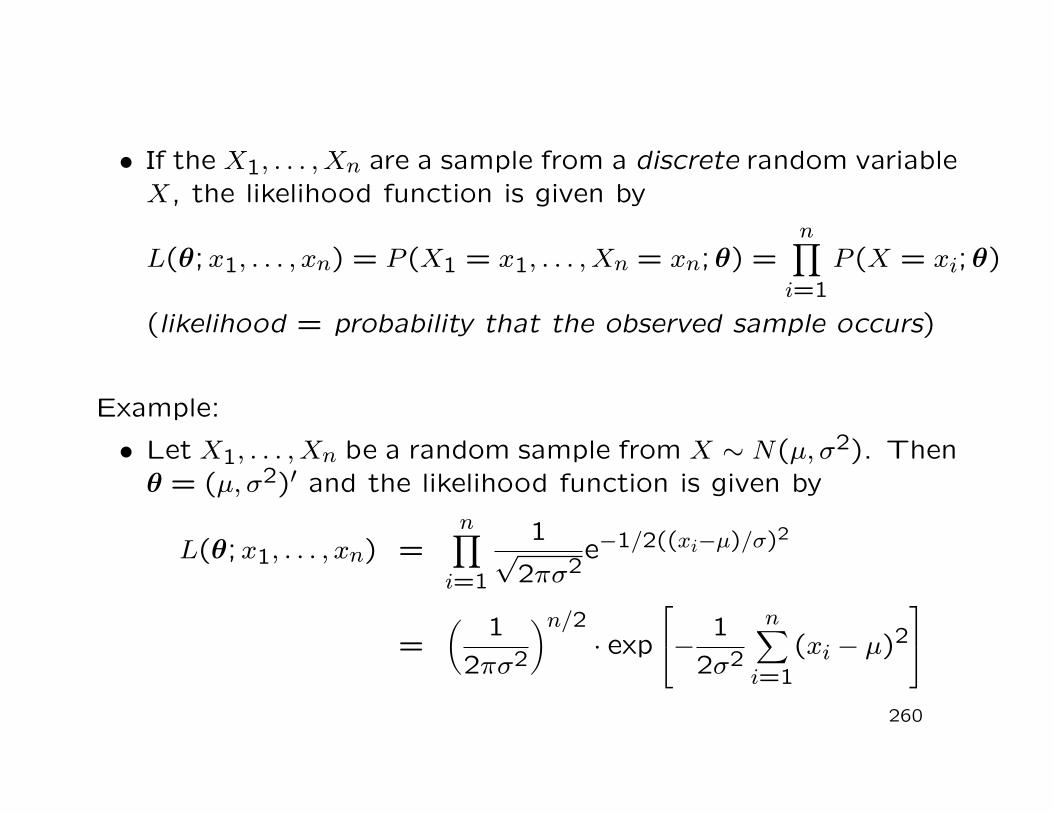
• If the X1, . . . , Xn are a sample from a discrete random variableX, the likelihood function is given by

L(θ;x1, . . . , xn) = P (X1 = x1, . . . , Xn = xn; θ) =n∏

i=1P (X = xi; θ)

(likelihood = probability that the observed sample occurs)

Example:

• Let X1, . . . , Xn be a random sample from X ∼ N(µ, σ2). Thenθ = (µ, σ2)′ and the likelihood function is given by

L(θ;x1, . . . , xn) =n∏

i=1

1√2πσ2

e−1/2((xi−µ)/σ)2

=( 12πσ2

)n/2· exp

−1

2σ2

n∑

i=1(xi − µ)2

260

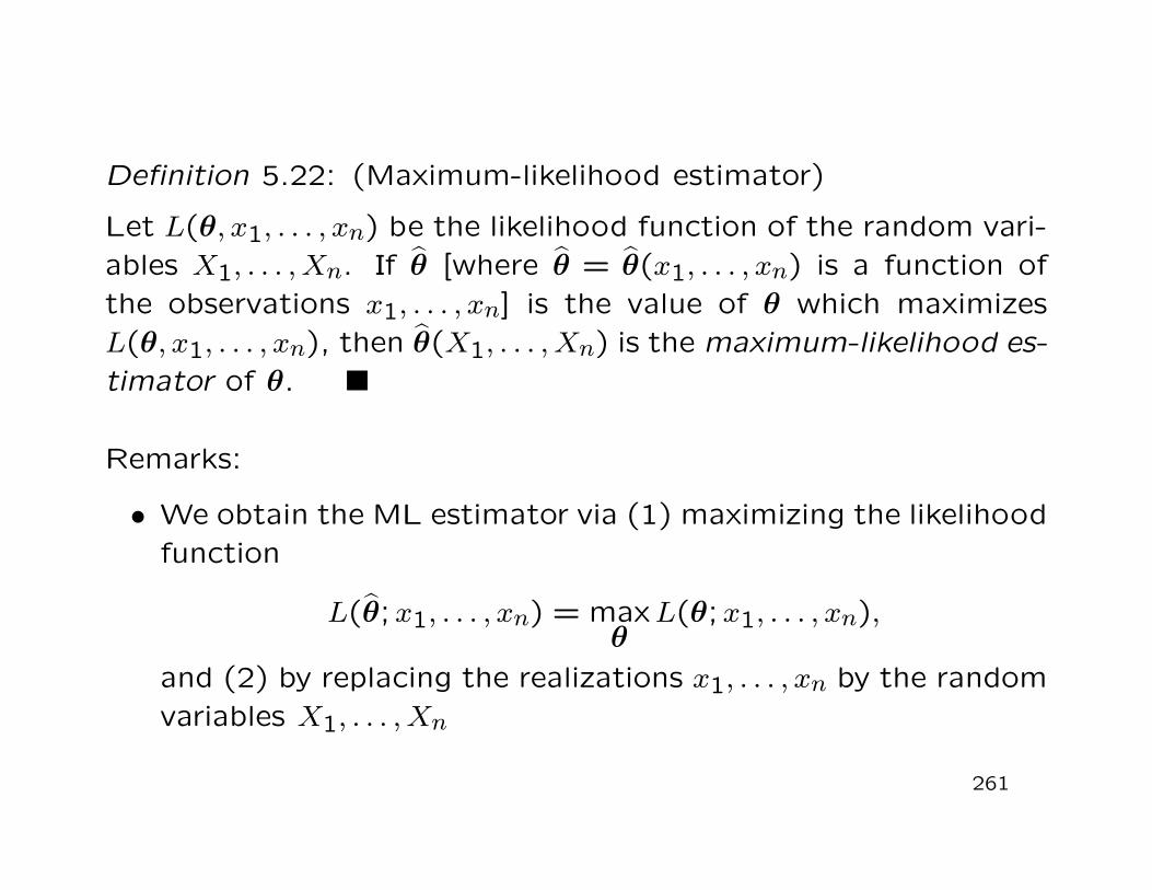
Definition 5.22: (Maximum-likelihood estimator)

Let L(θ, x1, . . . , xn) be the likelihood function of the random vari-ables X1, . . . , Xn. If θ [where θ = θ(x1, . . . , xn) is a function ofthe observations x1, . . . , xn] is the value of θ which maximizesL(θ, x1, . . . , xn), then θ(X1, . . . , Xn) is the maximum-likelihood es-timator of θ.

Remarks:

• We obtain the ML estimator via (1) maximizing the likelihoodfunction

L(θ;x1, . . . , xn) = maxθ

L(θ;x1, . . . , xn),

and (2) by replacing the realizations x1, . . . , xn by the randomvariables X1, . . . , Xn

261

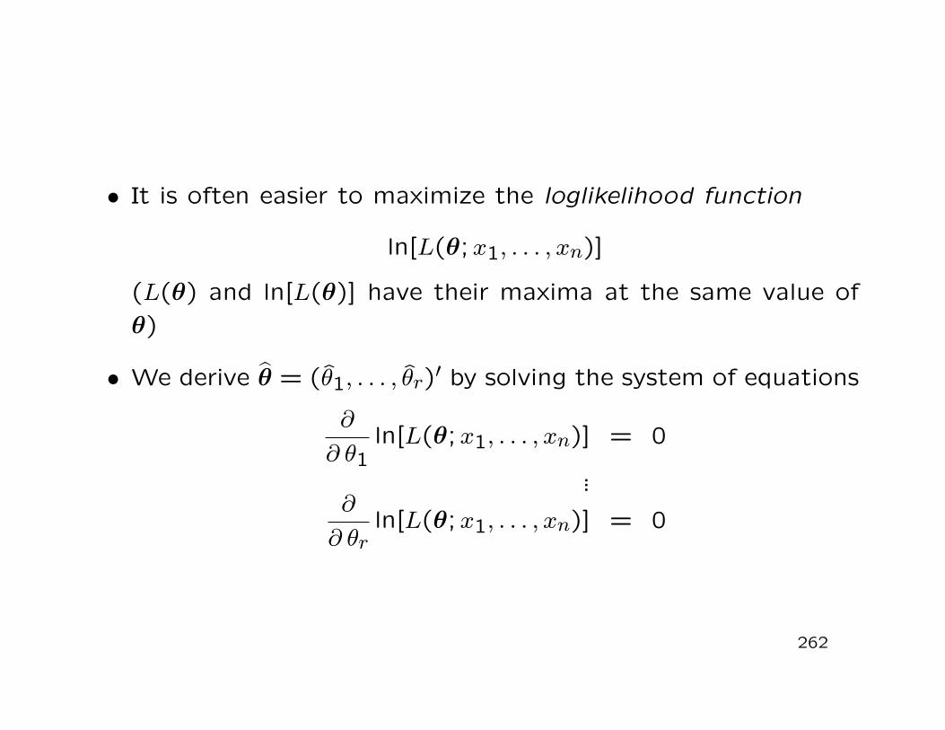
• It is often easier to maximize the loglikelihood function

ln[L(θ;x1, . . . , xn)]

(L(θ) and ln[L(θ)] have their maxima at the same value ofθ)

• We derive θ = (θ1, . . . , θr)′ by solving the system of equations

∂∂ θ1

ln[L(θ;x1, . . . , xn)] = 0

...∂

∂ θrln[L(θ;x1, . . . , xn)] = 0

262

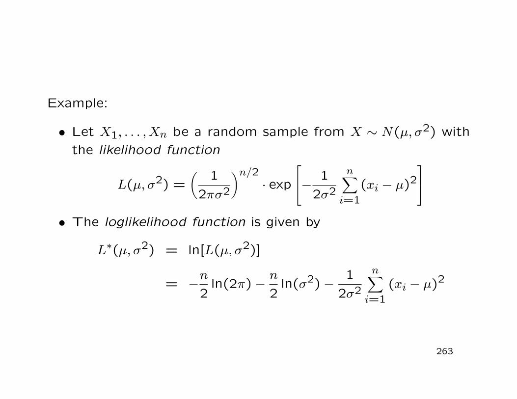
Example:

• Let X1, . . . , Xn be a random sample from X ∼ N(µ, σ2) withthe likelihood function

L(µ, σ2) =( 12πσ2

)n/2· exp

−1

2σ2

n∑

i=1(xi − µ)2

• The loglikelihood function is given by

L∗(µ, σ2) = ln[L(µ, σ2)]

= −n2

ln(2π)−n2

ln(σ2)−1

2σ2

n∑

i=1(xi − µ)2

263

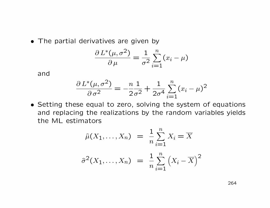
• The partial derivatives are given by

∂ L∗(µ, σ2)∂ µ

=1σ2

n∑

i=1(xi − µ)

and

∂ L∗(µ, σ2)∂ σ2 = −

n2

1σ2 +

12σ4

n∑

i=1(xi − µ)2

• Setting these equal to zero, solving the system of equationsand replacing the realizations by the random variables yieldsthe ML estimators

µ(X1, . . . , Xn) =1n

n∑

i=1Xi = X

σ2(X1, . . . , Xn) =1n

n∑

i=1

(

Xi −X)2

264

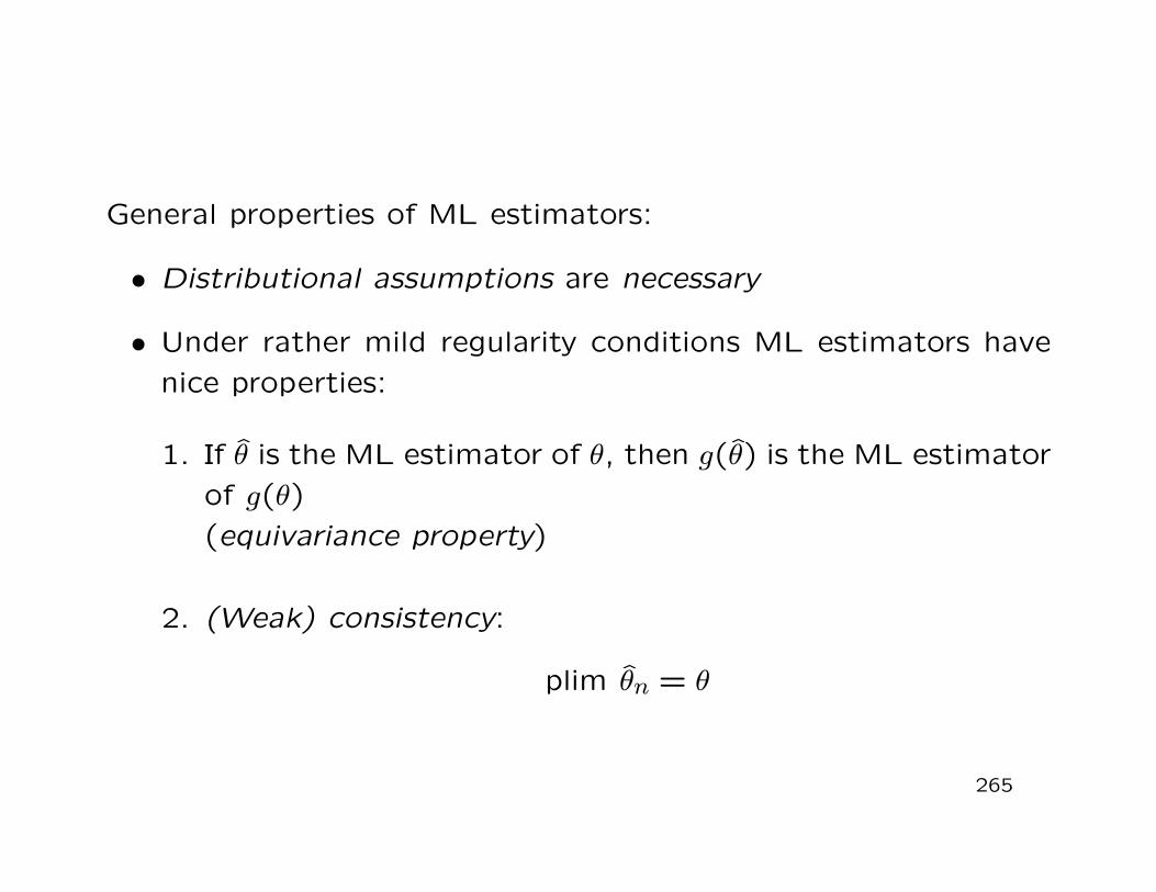
General properties of ML estimators:

• Distributional assumptions are necessary

• Under rather mild regularity conditions ML estimators havenice properties:

1. If θ is the ML estimator of θ, then g(θ) is the ML estimatorof g(θ)(equivariance property)

2. (Weak) consistency:

plim θn = θ

265

3. Asymptotic normality:√

n(

θn − θ) d→ U ∼ N(0, V (θ))

4. Asymptotic efficiency:V (θ) coincides with the Cramer-Rao lower bound

5. Direct computation (numerical methods)

6. Quasi-ML estimation:ML estimators computed on the basis of normally dis-tributed random samples are robust even if the randomsample actually is not normally distributed(robustness against distribution misspecification)

266

6. Hypothesis Testing

Setting:

• Let X represent the random experiment under consideration

• Let X have the unknown cdf FX(x)

• We are interested in an unknown parameter θ in the distri-bution of X

Now:

• Testing of a statistical hypothesis on the unknown θ on thebasis of a random sample X1, . . . , Xn

267

Example 1:

• In a our local pub the glasses are said to contain 0.4 litresof beer. We suspect that in many cases the glasses actuallycontain less than 0.4 litres of beer

• Let X represent the process of ’filling a glass of beer’

• Let θ = E(X) denote the expected amount of beer filled inone glass

• On the basis of a random sample X1, . . . , Xn we would liketo test

θ = 0.4 versus θ < 0.4

268

Example 2:

• We know from past data that the risk of a specific stock(measured by the standard deviation of the stock return) hasbeen equal to 25%. Now, there is a change in the managerialboard of the firm. Does this change affect the risk of thestock?

• Let X represent the stock return

• Let θ =√

Var(X) = SD(X) denote the standard deviation ofthe return

• On the basis of a random sample X1, . . . , Xn we would liketo test

θ = 0.25 versus θ 6= 0.25

269

6.1 Basic Terminology

Definition 6.1: (Parameter test)

Let X be a random variable and let θ be an unknown parameter inthe distribution of X. A parameter test constitutes a statisticalprocedure for deciding on a hypothesis concerning the unknownparameter θ on the basis of a random sample X1, . . . , Xn fromX.

Statistical hypothesis-testing problem:

• Let Θ denote the set of all possible parameter values(i.e. θ ∈ Θ; we call Θ the parameter space)

• Let Θ0 ⊂ Θ be a subset of the parameter space

270

• Consider the following statements:

H0 : θ ∈ Θ0 versus H1 : θ ∈ Θ/Θ0 = Θ1

• H0 is called the null hypothesis, H1 is called the alternativehypothesis

Types of hypotheses:

• If |Θ0| = 1 (i.e. Θ0 = θ0) and H0 : θ = θ0, then H0 is calledsimple

• Otherwise H0 is called composite

• An analogous terminology applies to H1

271

Types of hypothesis tests:

• Let θ0 ∈ Θ be a real constant. Then

H0 : θ = θ0 versus H1 : θ 6= θ0

is called a two-sided test

• The tests

H0 : θ ≤ θ0 versus H1 : θ > θ0

and

H0 : θ ≥ θ0 versus H1 : θ < θ0

are called one-sided tests (right- and left-sided tests)

272

Next:• Consider the general testing problem

H0 : θ ∈ Θ0 versus H1 : θ ∈ Θ1 = Θ/Θ0

General procedure:• Based on a random sample X1, . . . , Xn from X decide on

whether to reject H0 in favor of H1 or not

Explicit procedure:• Select an ’appropriate’ test statistic T (X1, . . . , Xn) and de-

termine an ’appropriate’ critical region K ⊂ R• Decision:

T (X1, . . . , Xn) ∈ K =⇒ reject H0T (X1, . . . , Xn) /∈ K =⇒ do not reject (accept) H0

273

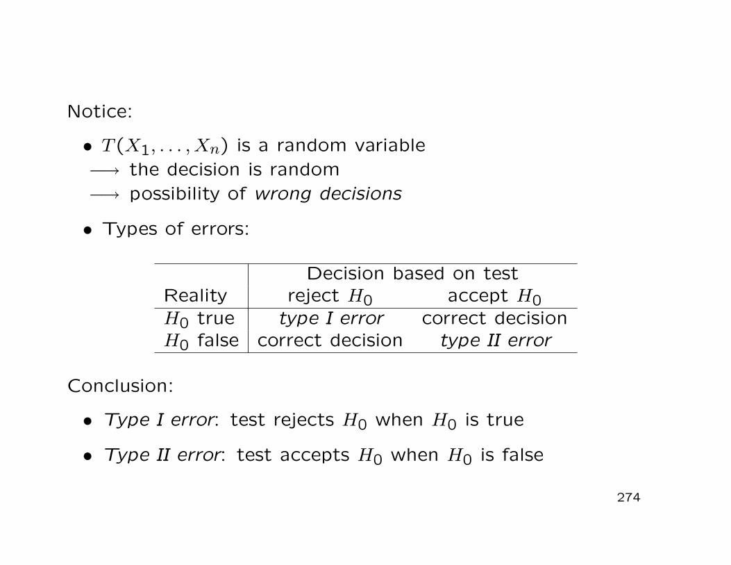
Notice:

• T (X1, . . . , Xn) is a random variable−→ the decision is random−→ possibility of wrong decisions

• Types of errors:

Decision based on testReality reject H0 accept H0H0 true type I error correct decisionH0 false correct decision type II error

Conclusion:

• Type I error: test rejects H0 when H0 is true

• Type II error: test accepts H0 when H0 is false

274

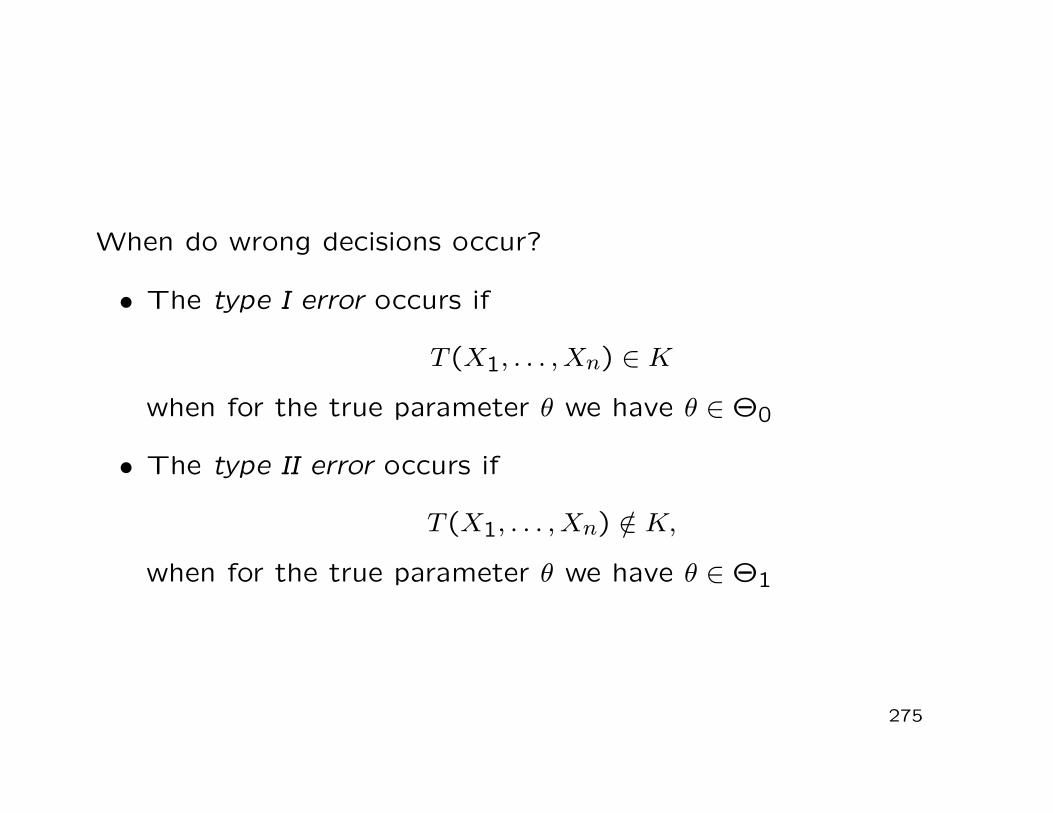
When do wrong decisions occur?

• The type I error occurs if

T (X1, . . . , Xn) ∈ K

when for the true parameter θ we have θ ∈ Θ0

• The type II error occurs if

T (X1, . . . , Xn) /∈ K,

when for the true parameter θ we have θ ∈ Θ1

275

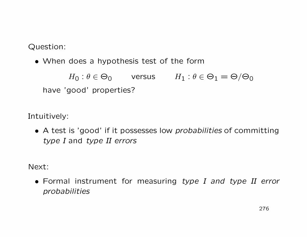
Question:

• When does a hypothesis test of the form

H0 : θ ∈ Θ0 versus H1 : θ ∈ Θ1 = Θ/Θ0

have ’good’ properties?

Intuitively:

• A test is ’good’ if it possesses low probabilities of committingtype I and type II errors

Next:

• Formal instrument for measuring type I and type II errorprobabilities

276

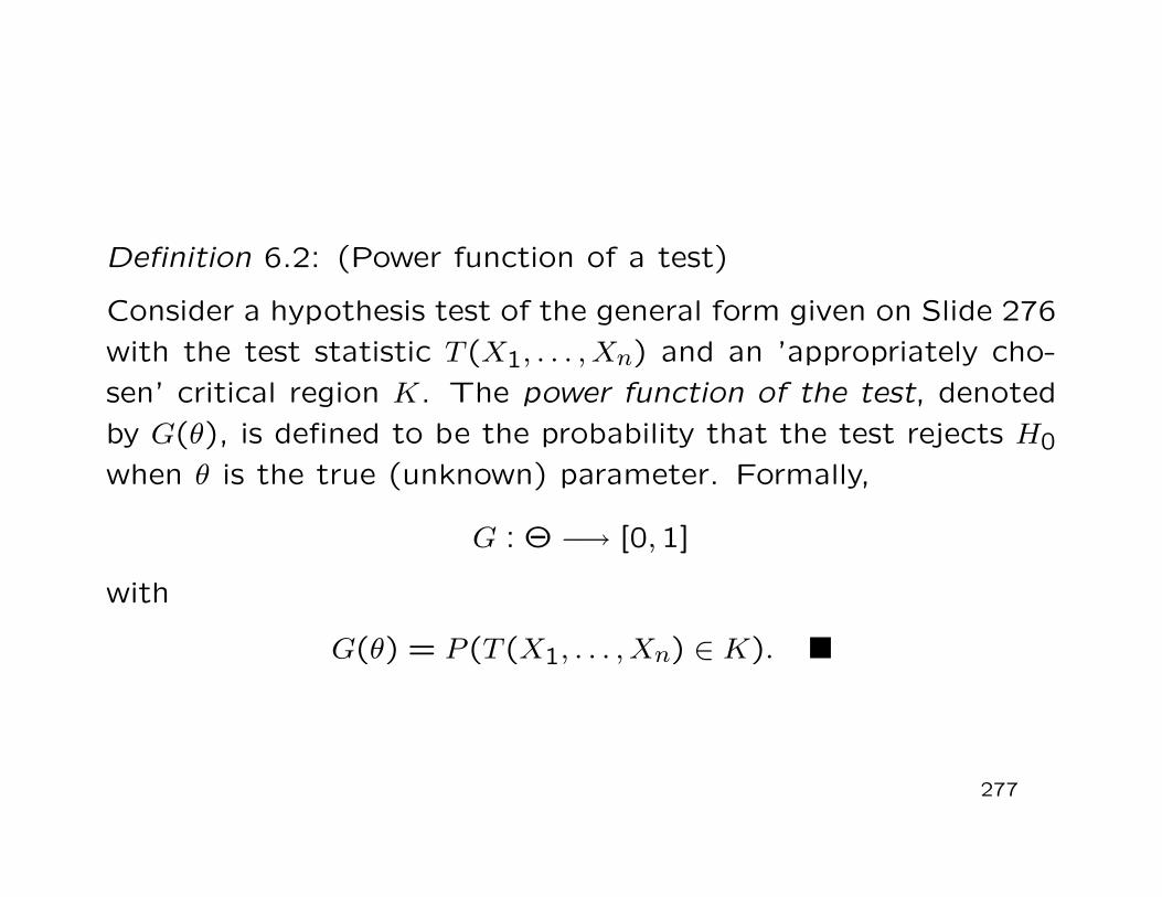
Definition 6.2: (Power function of a test)

Consider a hypothesis test of the general form given on Slide 276with the test statistic T (X1, . . . , Xn) and an ’appropriately cho-sen’ critical region K. The power function of the test, denotedby G(θ), is defined to be the probability that the test rejects H0when θ is the true (unknown) parameter. Formally,

G : Θ −→ [0,1]

with

G(θ) = P (T (X1, . . . , Xn) ∈ K).

277

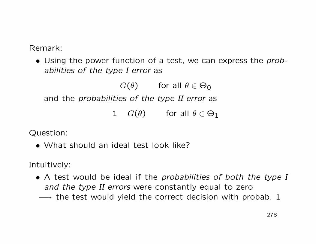
Remark:

• Using the power function of a test, we can express the prob-abilities of the type I error as

G(θ) for all θ ∈ Θ0

and the probabilities of the type II error as

1−G(θ) for all θ ∈ Θ1

Question:

• What should an ideal test look like?

Intuitively:

• A test would be ideal if the probabilities of both the type Iand the type II errors were constantly equal to zero−→ the test would yield the correct decision with probab. 1

278

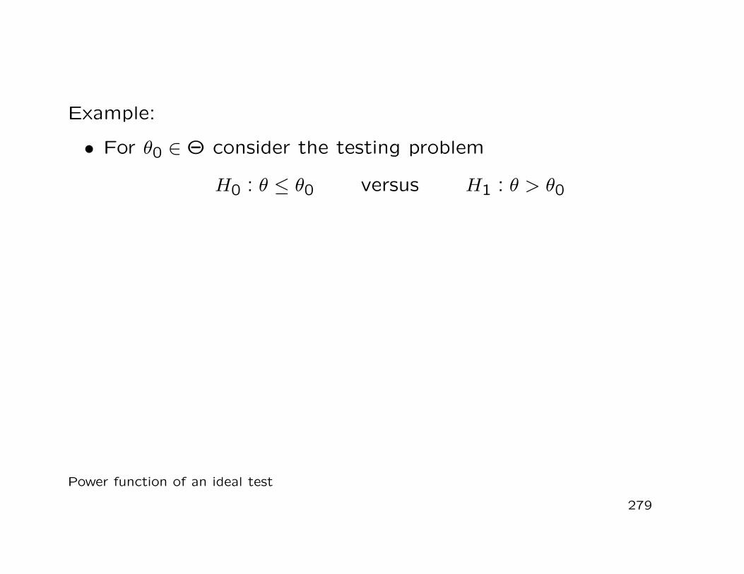
Example:

• For θ0 ∈ Θ consider the testing problem

H0 : θ ≤ θ0 versus H1 : θ > θ0

Power function of an ideal test

279

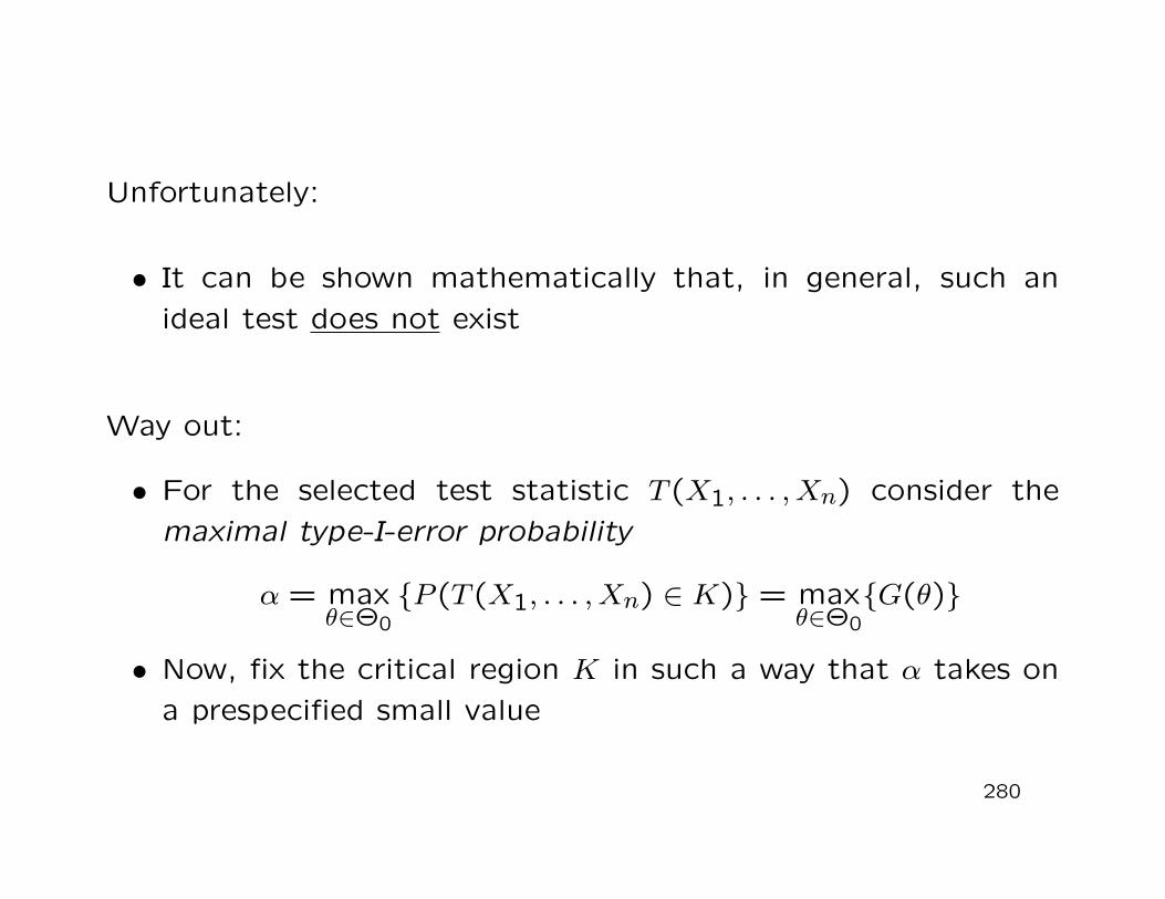
Unfortunately:

• It can be shown mathematically that, in general, such anideal test does not exist

Way out:

• For the selected test statistic T (X1, . . . , Xn) consider themaximal type-I-error probability

α = maxθ∈Θ0

P (T (X1, . . . , Xn) ∈ K) = maxθ∈Θ0

G(θ)

• Now, fix the critical region K in such a way that α takes ona prespecified small value

280

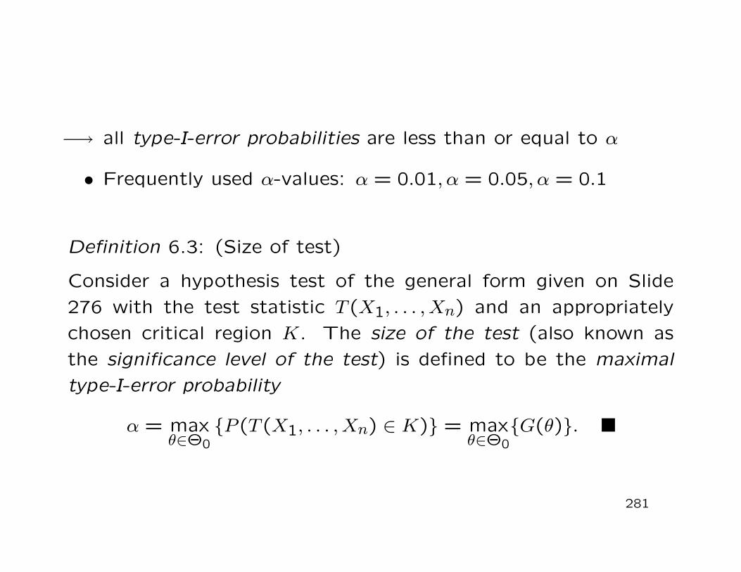
−→ all type-I-error probabilities are less than or equal to α

• Frequently used α-values: α = 0.01, α = 0.05, α = 0.1

Definition 6.3: (Size of test)

Consider a hypothesis test of the general form given on Slide276 with the test statistic T (X1, . . . , Xn) and an appropriatelychosen critical region K. The size of the test (also known asthe significance level of the test) is defined to be the maximaltype-I-error probability

α = maxθ∈Θ0

P (T (X1, . . . , Xn) ∈ K) = maxθ∈Θ0

G(θ).

281

Implications of this test construction:

• The probability of the test rejecting H0 when in fact H0 istrue (i.e. the type-I-error probability) is α at the utmost−→ if, for a concrete sample, the test rejects H0, we can be

quite sure that H0 is in fact false(we say that H1 is statistically significant)

• By contrast, we cannot control for the type-II-error proba-bility (i.e. for the probability of the test accepting H0 whenin fact H0 is false)−→ if, for a concrete sample, the test accepts H0, then there

is no probability assessment of a potentially wrong deci-sion(acceptance of H0 simply means: the data are not incon-sistent with H0)

282

Therefore:

• It is crucial how to formulate H0 and H1

• We formulate our research hypothesis in H1(hoping that, for a concrete sample, our test rejects H0)

Example:

• Consider Example 1 on Slide 268

• If, for a concrete sample, our test rejects H0 we can be quitesure that (on average) the glasses contain less than 0.4 litresof beer

• If our test accepts H0 we cannot make a statistically signifi-cant statement(the data are not inconsistent with H0)

283

6.2 Classical Testing Procedures

Next:

• Three general classical testing procedures based on the log-likelihood function of a random sample

Setting:

• Let X1, . . . , Xn be a random sample from X

• Let θ ∈ R be an unknown parameter

• Let L(θ) = L(θ;x1, . . . , xn) denote the likelihood function

284

• Let ln[L(θ)] denote the loglikelihood function

• Assume g : R −→ R to be a continuous function

• Consider the testing problem:

H0 : g(θ) = q versus H1 : g(θ) 6= q

Fundamental to all three tests:

• Maximum-Likelihood estimator θML of θ

285

6.2.1 Wald Test

History:

• Suggested by A. Wald (1902-1950)

Idea behind this test:

• If H0 : g(θ) = q is true, then the random variable g(θML)− qshould not be significantly different from zero

286

Previous knowledge:

• Equivariance property of the ML estimator (Slide 265)−→ g(θML) is the ML estimator of g(θ)

• Asymptotic normality (Slide 266)

−→(

g(θML)− g(θ)) d→ U ∼ N(0,Var(g(θML)))

• The asymptotic variance Var(g(θML)) needs to be estimatedfrom the data

Wald test statistic:

W =

[

g(

θML)

− q]2

Var[

g(

θML)]

d(under H0)−→ U ∼ χ2

1

287

Test decision:

• Reject H0 at the significance level α if W > χ21;1−α

Remarks:

• The Wald test is a pure test against H0(it is not necessary to exactly specify H1)

• The Wald principle can be applied to any consistent, asymp-totically normally distributed estimator

288

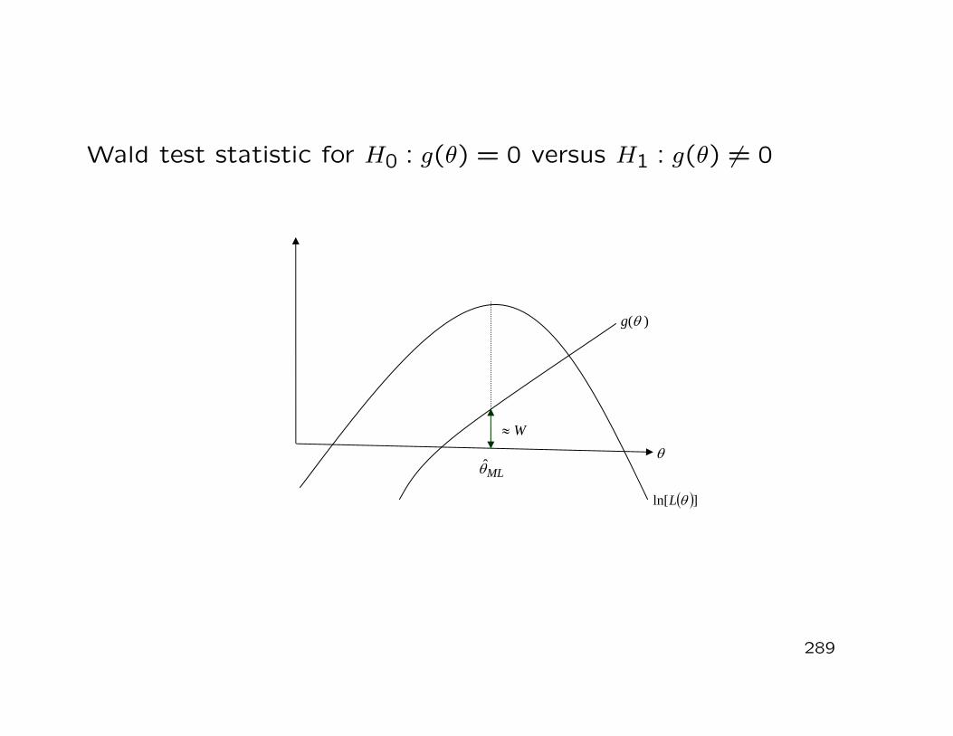
Wald test statistic for H0 : g(θ) = 0 versus H1 : g(θ) 6= 0

289

g(θ )

≈ Wθ

MLθ

( )]ln[ θL

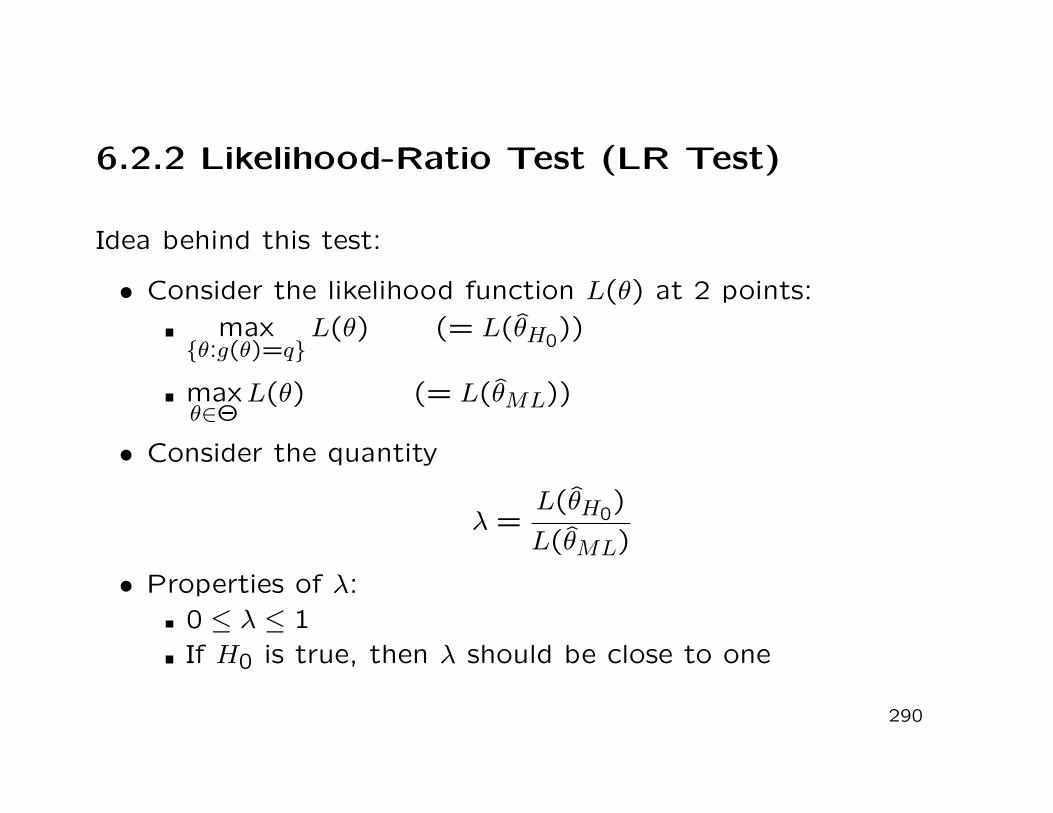
6.2.2 Likelihood-Ratio Test (LR Test)

Idea behind this test:

• Consider the likelihood function L(θ) at 2 points:max

θ:g(θ)=qL(θ) (= L(θH0))

maxθ∈Θ

L(θ) (= L(θML))

• Consider the quantity

λ =L(θH0)

L(θML)

• Properties of λ:0 ≤ λ ≤ 1If H0 is true, then λ should be close to one

290

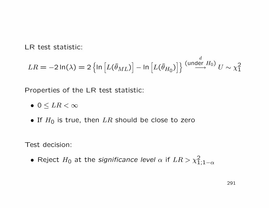
LR test statistic:

LR = −2 ln(λ) = 2

ln[

L(θML)]

− ln[

L(θH0)]

d(under H0)−→ U ∼ χ2

1

Properties of the LR test statistic:

• 0 ≤ LR < ∞

• If H0 is true, then LR should be close to zero

Test decision:

• Reject H0 at the significance level α if LR > χ21;1−α

291

Remarks:

• The LR test verifies if the distance in the loglikelihood func-tions, ln[L(θML)]− ln[L(θH0)], is significantly larger than 0

• The LR test does not require the computation of any asymp-totic variance

292

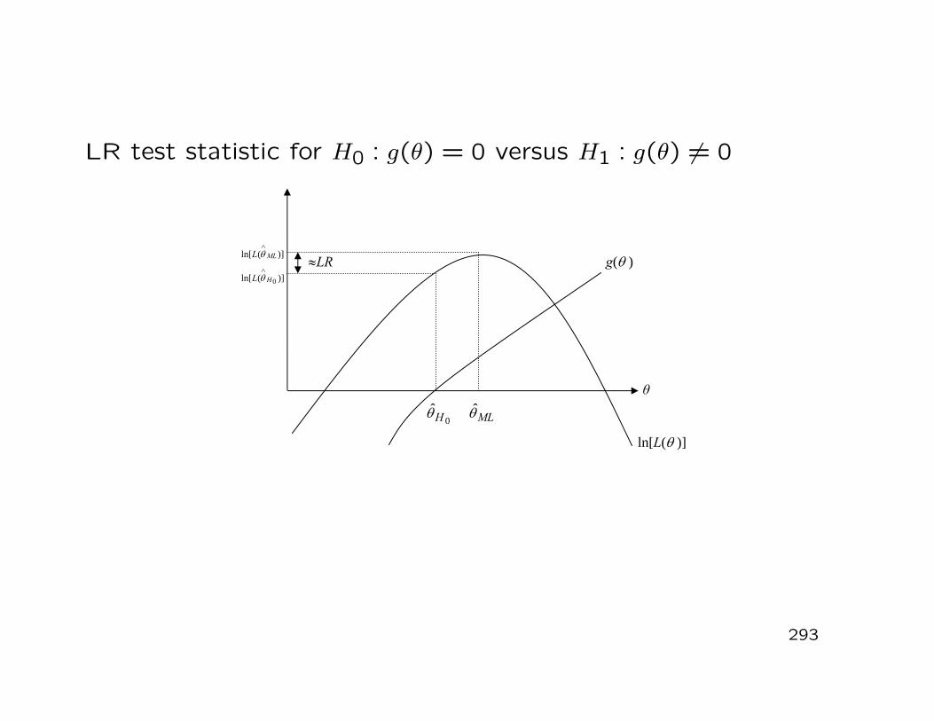
LR test statistic for H0 : g(θ) = 0 versus H1 : g(θ) 6= 0

293

)](ln[ MLL∧θ g(θ ) g(θ ) ≈LR

)](ln[ 0HL∧θ

θ

MLθ0

ˆHθ

ln[L(θ )]

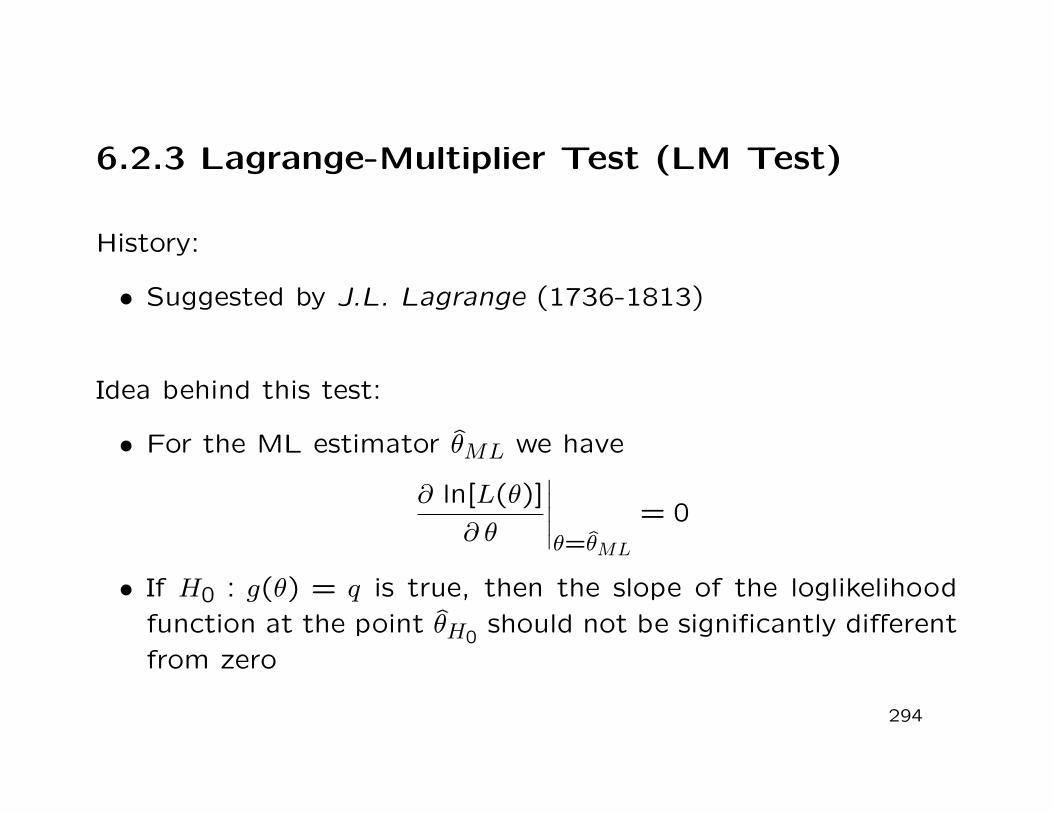
6.2.3 Lagrange-Multiplier Test (LM Test)

History:

• Suggested by J.L. Lagrange (1736-1813)

Idea behind this test:

• For the ML estimator θML we have

∂ ln[L(θ)]∂ θ

∣

∣

∣

∣

∣

θ=θML

= 0

• If H0 : g(θ) = q is true, then the slope of the loglikelihoodfunction at the point θH0 should not be significantly differentfrom zero

294

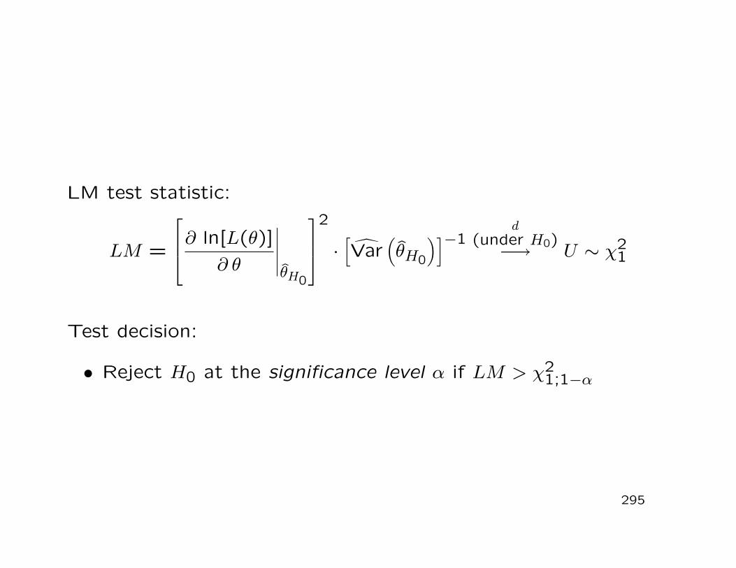
LM test statistic:

LM =

∂ ln[L(θ)]∂ θ

∣

∣

∣

∣

∣

θH0

2

·[

Var(

θH0

)]−1d

(under H0)−→ U ∼ χ21

Test decision:

• Reject H0 at the significance level α if LM > χ21;1−α

295

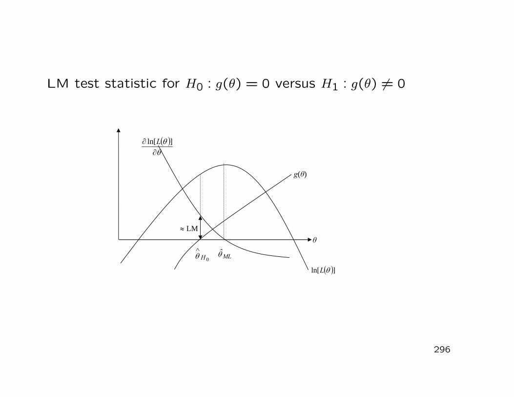
LM test statistic for H0 : g(θ) = 0 versus H1 : g(θ) 6= 0

296

( )θθ

∂∂ ]ln[L

MLθ

( )]ln[ θL

≈ LM θ

g(θ)

0H∧θ

Remarks:

• The test statistics of both, the Wald and the LM tests, con-tain the estimated variances of the estimator θH0

• These unknown variances can be estimated consistently bythe co-called Fisher-information

• Many econometric tests are based on these three construc-tion principles

• The three tests are asymptotically equivalent, i.e. for largesample sizes they produce identical test decisions

• The three principles can be extended to the testing of hy-potheses on a parameter vector θ

• If θ ∈ Rm, then all 3 test statistics have a χ2m distribution

under H0

297

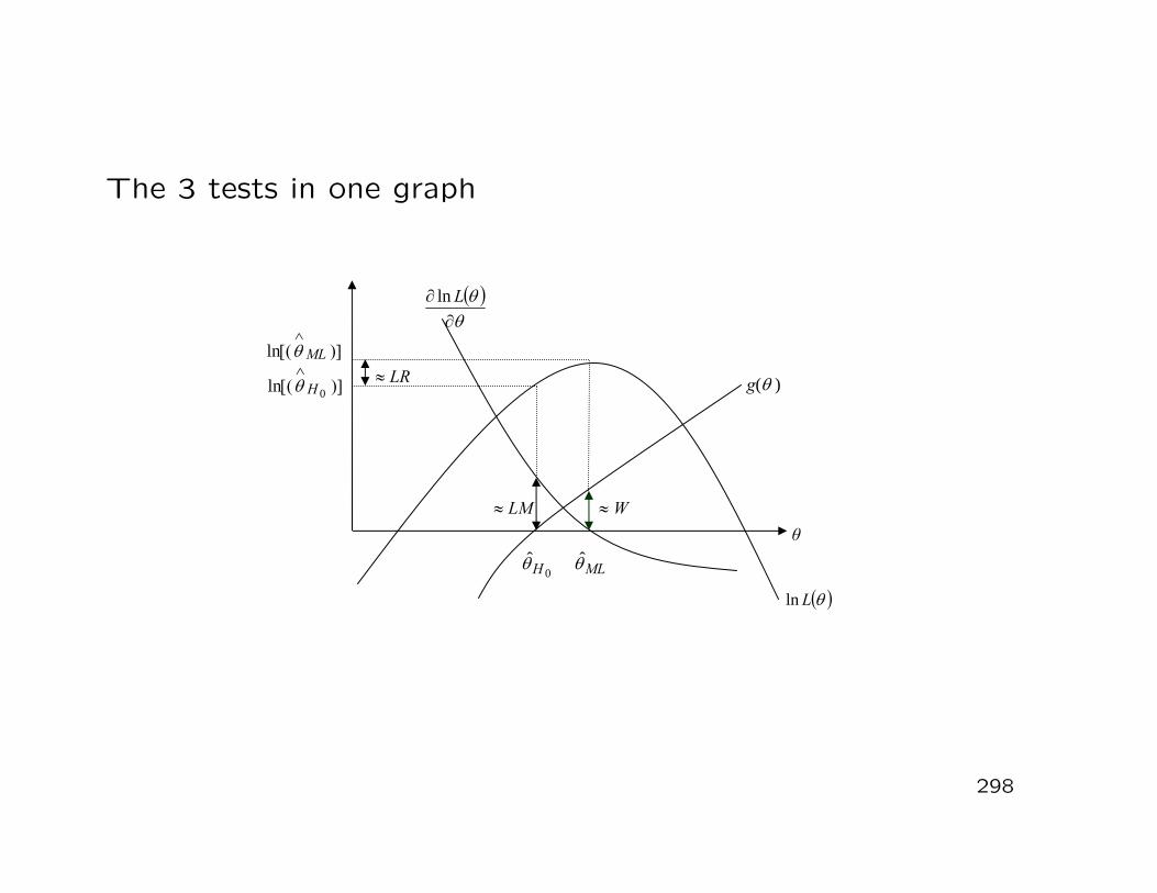
The 3 tests in one graph

298

( )

θθ

∂∂ Lln

ln[( )] ML∧θ

ln[( )] 0H∧θ ≈ LR g(θ )

≈ LM ≈ Wθ

MLθ0

ˆHθ

( )θLln