Section 12.2-1 Copyright © 2014, 2012, 2010 Pearson Education, Inc. Lecture Slides Elementary Statistics Twelfth Edition and the Triola Statistics Series

Section 12.2-1Copyright © 2014, 2012, 2010 Pearson Education, Inc.

Lecture Slides

Elementary Statistics Twelfth Edition

and the Triola Statistics Series

by Mario F. Triola


Chapter 12Analysis of Variance

12-1 Review and Preview

12-2 One-Way ANOVA

12-3 Two-Way ANOVA


Key Concept

This section introduces the method of one-way analysis of variance, which is used for tests of hypotheses that three or more population means are all equal.

Because the calculations are very complicated, we emphasize the interpretation of results obtained by using technology.


Key Concept

1. Understand that a small P-value (such as 0.05 or less) leads to rejection of the null hypothesis of equal means.

With a large P-value (such as greater than 0.05), fail to reject the null hypothesis of equal means.

2. Develop an understanding of the underlying rationale by studying the examples in this section.


Part 1: Basics of One-Way Analysis of Variance


Definition

One-way analysis of variance (ANOVA) is a method of testing the equality of three or more population means by analyzing sample variances.

One-way analysis of variance is used with data categorized with one factor (or treatment), which is a characteristic that allows us to distinguish the different populations from one another.


One-Way ANOVARequirements

1. The populations have approximately normal distributions.

2. The populations have the same variance σ2 (or standard deviation σ).

3. The samples are simple random samples of quantitative data.

4. The samples are independent of each other.

5. The different samples are from populations that are categorized in only one way.


Procedure

1. Use STATDISK, Minitab, Excel, StatCrunch, a TI-83/84 calculator, or any other technology to obtain results.

2. Identify the P-value from the display.

3. Form a conclusion based on these criteria:

If the P-value ≤ α, reject the null hypothesis of equal means. Conclude at least one mean is different from the others.

If the P-value > α, fail to reject the null hypothesis of equal means.

0 1 2 3To test : kH μ μ μ μ= = = =L


Caution

When we conclude that there is sufficient evidence to reject the claim of equal population means, we cannot conclude from ANOVA that any particular mean is different from the others.

There are several other tests that can be used to identify the specific means that are different, and some of them are discussed in Part 2 of this section.


Example

Use the performance IQ scores listed in Table 12-1 and a significance level of α = 0.05 to test the claim that the three samples come from populations with means that are all equal.


Example - Continued

Here are summary statistics from the collected data:


Example - Continued

Requirement Check:

1.The three samples appear to come from populations that are approximately normal (normal quantile plots OK).

2.The three samples have standard deviations that are not dramatically different.

3.We can treat the samples as simple random samples.

4.The samples are independent of each other and the IQ scores are not matched in any way.

5.The three samples are categorized according to a single factor: low lead, medium lead, and high lead.


Example - Continued

The hypotheses are:

The significance level is α = 0.05.

Technology results are presented on the next slides.

H0

: μ1 =μ2 =μ3

H1 : At least one of the means is different from the others.


Example - Continued


Example - Continued


Example - Continued


Example - Continued

The displays all show that the P-value is 0.020 when rounded.

Because the P-value is less than the significance level of α = 0.05, we can reject the null hypothesis.

There is sufficient evidence that the three samples come from populations with means that are different.

We cannot conclude formally that any particular mean is different from the others, but it appears that greater blood lead levels are associated with lower performance IQ scores.


P-Value and Test StatisticLarger values of the test statistic result in smaller P-values, so the ANOVA test is right-tailed.

The figure on the next slide shows the relationship between the F test statistic and the P-value.

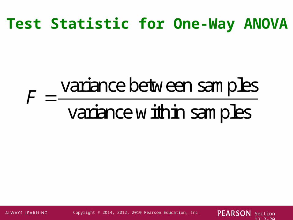
Assuming that the populations have the same variance σ2 (as required for the test), the F test statistic is the ratio of these two estimates of σ2:

• variation between samples (based on variation among sample means)

• variation within samples (based on the sample variances).


Relationship Between F Test Statistic and P-Value


Test Statistic for One-Way ANOVA

variance between samples

variance within samplesF =


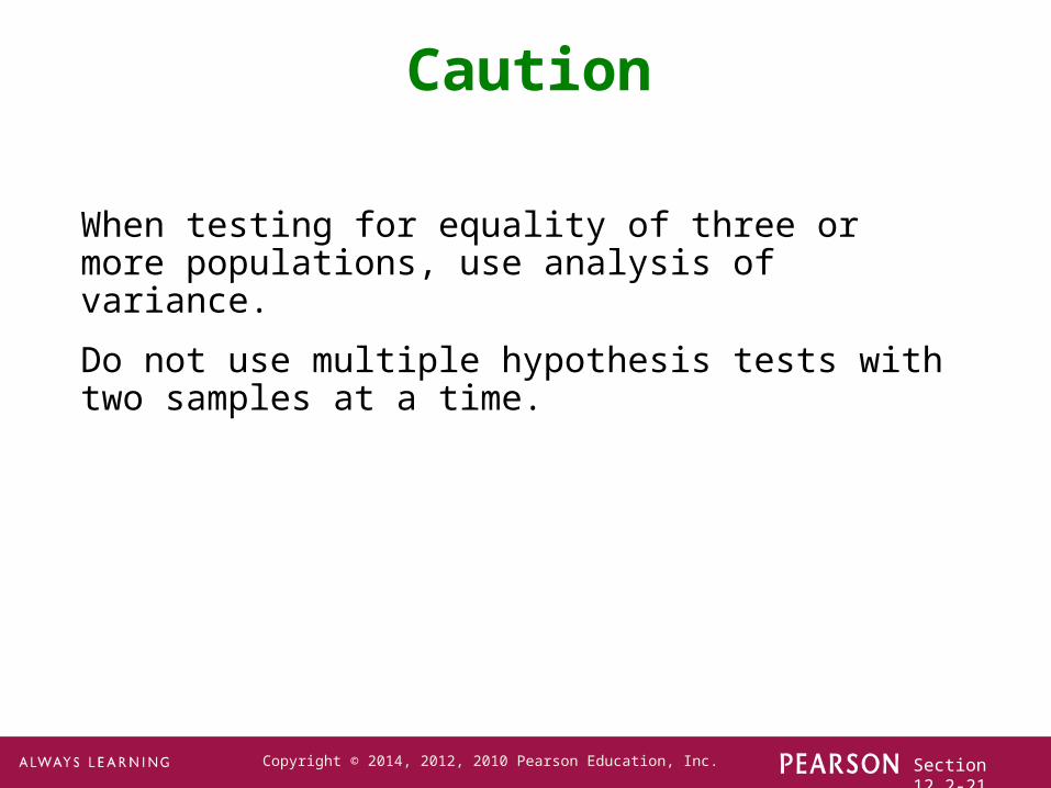
Caution

When testing for equality of three or more populations, use analysis of variance.

Do not use multiple hypothesis tests with two samples at a time.


Part 2: Calculations and Identifying Means That Are Different


Calculations with Equal or Unequal Sample Sizes

The text beginning on page 605 provides a detailed discussion on the calculations and ramifications of sample size for the F statistic.

As the material doesn’t lend itself to clean PowerPoint slides, we leave it to the reader to reference the main text.


Designing the Experiment

When performing ANOVA, we use one factor as the basis for partitioning the data into several categories.

If we conclude that there is a significant difference among means, we can’t be absolutely certain the differences are explained by the factor being used.

One way to reduce the effect of extraneous factors is to run a completely randomized design, in which each sample value is given the same chance of belonging to different factor groups.

Another way to reduce the effect of extraneous factors is to use a rigorously controlled design, in which sample values are carefully chosen so that all other factors have no variability.


Identifying Which Means Are Different

After conducting ANOVA, there are several informal methods for determining which means are different:

•Construct boxplots of the different samples to see if one or more of them is very different from the others.

•Construct confidence interval estimates of the means for the different samples, then compare those confidence intervals to see if one or more of them does not overlap with the others.


Identifying Which Means Are Different

There are several formal procedures to determine which means are different.

•Range tests allow us to identify subsets of means that are not significantly different from each other.

•Multiple comparison tests use pairs of means, making adjustments to overcome the problem of having a significance level that increases as the number of tests increases.

•There are many multiple comparisons tests, we introduce just one: The Bonferroni Multiple Comparison Test.


Bonferroni Multiple Comparison Test

Step 1: Do a separate t test for each pair of samples, but make the following adjustments:

Step 2: Use the value of MS(error), which uses all available sample data, as an estimate for the variance σ2. This value is obtained when conducting ANOVA.

Calculate the test statistic:

1 2

1 2

1 1MS(error)

x xt

n n

−=

⎛ ⎞+⎜ ⎟

⎝ ⎠g


Bonferroni Multiple Comparison Test

Step 3: Make the following adjustments:

P-value:Use the test statistic t with df = N – k, where N is the total number of sample values and k is the number of samples. Find the P-value as per usual, but adjust the P-value by multiplying it by the number of different possible pairings of two samples (e.g. with three samples, there are three possible pairings, so multiply by 3).

Critical Value: When finding the critical value, adjust α by dividing it by the number of possible pairings of two samples.


Example

We previously concluded, for the IQ score test, that there is sufficient evidence to warrant rejection of the claim of equal means.

Use the Bonferroni test with a 0.05 level of significance to identify which mean is different from the others.


Example - Continued

The null hypotheses to be tested are:

We begin with the first, and using the sample data presented earlier, arrive at (using technology):

0 1 2 0 1 3 0 2 3: : : H H Hμ μ μ μ μ μ= = =

1 1

2 2

78 102.705128

22 94.136364

MS(error) 248.424127

n x

n x

= =

= =

=


Example - Continued

The test statistic:

1 2

1 2

1 1MS(error)

102.705128 94.1363642.252

1 1248.424127

78 22

x xt

n n

−=

⎛ ⎞+⎜ ⎟

⎝ ⎠

−= =

⎛ ⎞+⎜ ⎟⎝ ⎠

g

g


Example - Continued

The test statistic of t = 2.252 has N – k = 121 – 3 = 118 df.

The two-tailed P-value is 0.026172, but it needs to be multiplied by 3 because there are three possible pairing of sample means.

Thus, the P-value = 0.079 rounded.

Because this P-value is not small (less than 0.05), we fail to reject the null hypothesis.

It appears that Samples 1 and 2 do not have significantly different means.


Example - Continued

Technology can display Bonferroni test results:


Example - Continued

Conclusion:

Although the ANOVA test tells us that at least one of the sample means is different from the others, the Bonferroni test results do not identify any one particular sample mean that is significantly different from the others.

Documents

Section 12.2-1 Copyright © 2014, 2012, 2010 Pearson Education, Inc. Lecture Slides Elementary Statistics Twelfth Edition and the Triola Statistics Series