Skills, Income Distribution, and the Size

Distribution of Fims∗

Matias Busso

IADB

mbusso AT iadb.org

Andy Neumeyer

UTDT

pan AT utdt.edu

Mariano Spector

UTDT

mspector AT utdt.edu

December 2014

Abstract

Cross-country evidence from the OECDs Programme for the International Assess-

ment of Adult Competencies (PIAAC) and from Latin American Household Surveys

supports the hypothesis that the skills of both employers and employees are positively

correlated with �rm size. This is true measuring skills either by cognitive abilities,

years of education, or relative earnings. Employees in large �rms earn more than small

entrepreneurs. Conditional on �rm size, entrepreneurs are more skilled and earn more

than employees�the distribution of earnings and abilities of entrepreneurs stochasti-

cally dominate the one for employees in similarly sized �rms.

We pose the question of whether the distribution of abilities can explain di�erences

in the size distribution of �rms between Mexico and the United States in a Lucas (1978)

model with two dimensions of ability and imperfect tax enforcement�a size dependent

policy. We calibrate abilities with a bi-variate log-normal distribution to match the

income distribution of entrepreneurs and of employees in each country. The model

successfully accounts for the size of �rms and informality in Mexico with a returns

to scale parameter of 0.66. For the US, the model simultaneously matches income

distribution in each occupation and �rm size only if the returns to scale parameter is

0.95.

∗We thank Francisco Buera, Nick Bloom, Hugo Hopenhayn, Pete Klenow, Santiago Levy, Hernán Ru�oand Pablo Sanguinetti for helpful conversations. All errors remain our own. Setfano Baratuche and JuanSebastián Muñoz provided excellent research assistance.

1 Introduction

The size distribution of �rms �is a topic on which issues of economic policy are

held to hinge: in wealthy economies, `bigness' is very widely viewed as a menace

against which government activity should, perhaps, be directed; in poor economies,

`littleness' as a sign of backwardness dealt with by government policy. The lack of

discipline with which such issues are typically discussed re�ects, I think, the lack

of an adequate understanding of the forces determining �rm size�Lucas (1978)

This paper is an attempt to understand cross country di�erences in the size distribution

of �rms. An example of the type of fact we want to explain is that 58% of employment in

Mexico is in �rms of less than 5 workers while in the united states 58% of employment is

in establishments of more the 100 workers. This is important because small �rms have a

relatively low total factor productivity and are informal�do not pay taxes. Hence countries

with many resources allocated to small �rms will have low aggregate total factor productivity

and large informal sectors.

The basic hypothesis we want to explore is that the size distribution of �rms is shaped by

the distribution of abilities across the population. Management practices in large corporations

demand more cognitive skills and non-cognitive skills from their employees than those in small

�rms.

We take this hypothesis to data using two homogeneous cross country datasets. The

OECDs Programme for the International Assessment of Adult Competencies (PIAAC)1 re-

leased in October 2014 and the Inter American Development Bank's harmonized house-

hold survey combined with UNESCOs Second Regional Comparative and Explanatory Study

(SERCE)2.

The cross-country evidence as well as the micro-data strongly supports the hypothesis

that the skills of both employers and employees are positively correlated with �rm size. This

is true measuring skills either by cognitive abilities, years of education, or relative earnings.

Employees in large �rms earn more than small entrepreneurs. Conditional on �rm size,

entrepreneurs are more skilled and earn more than employees�the distribution of earnings

and abilities of entrepreneurs stochastically dominate the one for employees in similarly sized

�rms.

Next, we develop the simplest model we can think of to link the distribution of skills with

1PIAAC is a survey of adult skills in which subjects are tested on numeracy, reading skills and asked aseries of questions on their demographic characteristics, labor market outcomes and characteristics of theirjobs and employers.

2Segundo Estudio regional Comparativo y Explicativo is an assessment of skills of elementary schoolstudents in Latin America.

1

the size distribution of �rms. We follow Lucas (1978) in using the Roy model of occupational

choice (Roy, 1951), as this is the standard model used in studies of the size distribution of

�rms. As the Lucas (1978) model with one dimensional skills implies that entrepreneurs

have higher incomes than employees, and in this is not true in the data, we add a second

dimension of heterogeneous ability to the agents in the model. Agents in our model di�er

in their entrepreneurial talent and in their ability as wage employees. We have in mind that

individuals di�er in their ability to work in teams, understand and respond to instructions,

be punctual, presentable and courteous, etc. The basic extension of the Lucas (1978) model

in this dimension is outlined in Jovanovic (1994). Agents choice between being workers or

entrepreneurs depends on their comparative advantage: the ratio between their individual

relative ability relative in the two occupations and the aggregate relative ability (after the

occupational choice is made). The size distribution of �rms depends, in turn, on the relative

ability as manager of each entrepreneurs relative to the aggregate ability of entrepreneurs.

These properties of the model imply that, in equilibrium, the size distribution of �rms and

occupational choices are homogeneous of degree zero in abilities.

Di�erences in the size distribution of �rms across countries may not be due to skills, but

to size dependent distortions (Hsieh and Klenow (2009), Guner, Ventura, and Yi (2008),

Buera). In order to allow for this type of distortions we introduce size dependent policies

in our simple model through the imperfect enforcement of payroll taxes�labor is the only

factor of production in our model. Firms are audited with a probability that is increasing

in the size of the �rm. The idea is that it is ine�cient for tax authorities to pay lawyers

and accountants to audit and prosecute myriads of poor small business owners and their

employees for evading taxes (see Bigio and Zilberman (2011)).

We quantitatively assess the model by contrasting it with data for Mexico and for the

United States. The main questions posed to the model is whether di�erences in the distribu-

tion of abilities can explain di�erences in the size distribution of �rms between Mexico and

the United States.

We assume abilities have a bi-variate log-normal distribution and a production function

with decreasing returns to scale. The model is calibrated using income distribution data for

entrepreneurs and employees to pin down the parameters of the log-normal distribution of

abilities. The enforcement technology is calibrated to match the degree of informality across

�rms of di�erent sizes in Mexico.

The model is very successful in accounting for the size distribution of �rms and for

informality in Mexico. In this exercise the returns to scale are calibrated to be 0.66, which

is consistent with the �rm curvature in Hsieh and Klenow (2009). However, when applied to

the United States the model with the same returns to scale parameter is unable to account

2

simultaneously for the income distribution of entrepreneurs and employees and for the size

distribution of �rms. The model successfully accounts for the US data on income distribution,

�rms size and tax evasion if the returns to scale parameter is set to 0.95. In this exercise the

enforcement technology is the same as in the Mexican case. The conclusion is that the Lucas

(1978) model of the size distribution of �rms with two dimensions of log-normally distributed

abilities calibrated to match income distribution data can only account for di�erences in �rm

sizes between Mexico and the United States if the returns to scale parameter changes.

There are two interpretations of the main quantitative result. The one we prefer is that

returns to scale depend on management practices, which in turn are dependent on abilities

(Bloom and Reenen (2007)). This implies that the next step in a research agenda linking the

size distribution of �rms and abilities is to model how abilities determine the returns to scale

(span of control) parameter. An alternative interpretation if one thinks the monopolistic

competition limits the size of �rms is that in the US markets are more competitive so that

�rms can be bigger.

The paper is organized as follows. Section 2 contains the empirical part of the paper,

presenting cross-country evidence in section 2.1 and data on Mexico and the United States

in section 2.2. The model is laid out in section 3. Section 4 explains the solution method and

calibration, section 5.2 has the main results and section 6 presents the concluding remarks.

2 Skills, Occupational Choice, and the Size Distribution

of Firms

This documents several empirical regularities on the relation between measures of abilities

and the size distribution of �rms across OECD regions and across Latin American countries.

We report the characteristics of individuals in di�erent occupations.

2.1 Cross Country Evidence

2.1.1 Cognitive Skills and Firm Size

In this section we report the relation between two measures of �rm size and aggregate mea-

sures of ability.

The �rst �nding is that �rm size is positively correlated with abilities. We establish this

for two di�erent measures of �rm size. First, for each OECD region and for each Latin

American country, we measure average �rm size by dividing the number of urban employees

in the private sector by the number of self-employed (with and without employees) in the

3

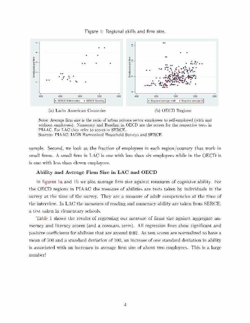
Figure 1: Regional skills and �rm size.

(a) Latin American Countries (b) OECD Regions

Note: Average �rm size is the ratio of urban private sector employees to self-employed (with andwithout employees). Numeracy and Reading in OECD are the scores for the respective tests inPIAAC. For LAC they refer to scores in SERCE.Sources: PIAAC, IADB Harmonized Household Surveys and SERCE.

sample. Second, we look at the fraction of employees in each region/country that work in

small �rms. A small �rm in LAC is one with less than six employees while in the OECD it

is one with less than eleven employees.

Ability and Average Firm Size in LAC and OECD

In �gures 1a and 1b we plot average �rm size against measures of cognitive ability. For

the OECD regions in PIAAC the measure of abilities are tests taken by individuals in the

survey at the time of the survey. They are a measure of adult competencies at the time of

the interview. In LAC the measures of reading and numeracy ability are taken from SERCE,

a test taken in elementary schools.

Table 1 shows the results of regressing our measure of �rms size against aggregate nu-

meracy and literacy scores (and a constant term). All regression lines show signi�cant and

positive coe�cients for abilities that are around 0.02. As test scores are normalized to have a

mean of 500 and a standard deviation of 100, an increase of one standard deviation in ability

is associated with an increases in average �rm size of about two employees. This is a large

number!

4

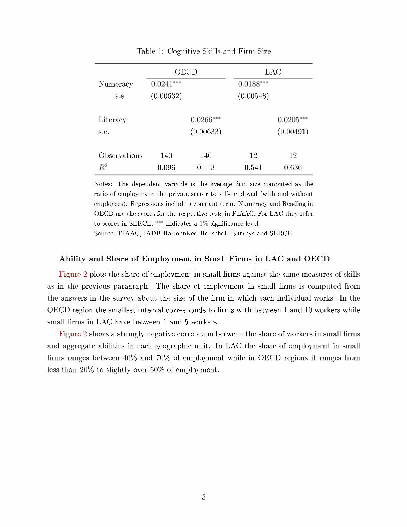
Table 1: Cognitive Skills and Firm Size

OECD LAC

Numeracy 0.0241∗∗∗ 0.0188∗∗∗

s.e. (0.00632) (0.00548)

Literacy 0.0266∗∗∗ 0.0205∗∗∗

s.e. (0.00633) (0.00491)

Observations 140 140 12 12

R2 0.096 0.113 0.541 0.636

Notes: The dependent variable is the average �rm size computed as the

ratio of employees in the private sector to self-employed (with and without

employees). Regressions include a constant term. Numeracy and Reading in

OECD are the scores for the respective tests in PIAAC. For LAC they refer

to scores in SERCE. ∗∗∗ indicates a 1% signi�cance level.

Source: PIAAC, IADB Harmonized Household Surveys and SERCE.

Ability and Share of Employment in Small Firms in LAC and OECD

Figure 2 plots the share of employment in small �rms against the same measures of skills

as in the previous paragraph. The share of employment in small �rms is computed from

the answers in the survey about the size of the �rm in which each individual works. In the

OECD region the smallest interval corresponds to �rms with between 1 and 10 workers while

small �rms in LAC have between 1 and 5 workers.

Figure 2 shows a strongly negative correlation between the share of workers in small �rms

and aggregate abilities in each geographic unit. In LAC the share of employment in small

�rms ranges between 40% and 70% of employment while in OECD regions it ranges from

less than 20% to slightly over 50% of employment.

5

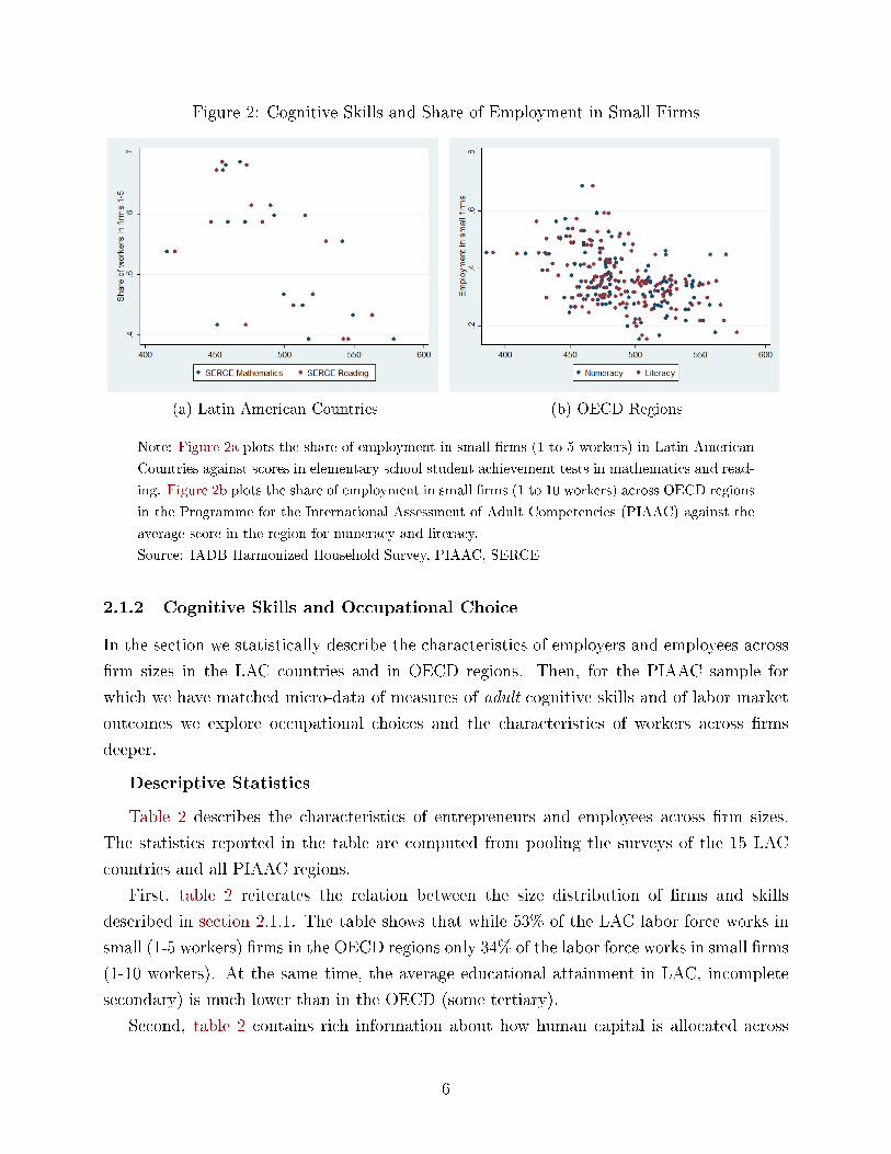
Figure 2: Cognitive Skills and Share of Employment in Small Firms

(a) Latin American Countries (b) OECD Regions

Note: Figure 2a plots the share of employment in small �rms (1 to 5 workers) in Latin American

Countries against scores in elementary school student achievement tests in mathematics and read-

ing. Figure 2b plots the share of employment in small �rms (1 to 10 workers) across OECD regions

in the Programme for the International Assessment of Adult Competencies (PIAAC) against the

average score in the region for numeracy and literacy.

Source: IADB Harmonized Household Survey, PIAAC, SERCE

2.1.2 Cognitive Skills and Occupational Choice

In the section we statistically describe the characteristics of employers and employees across

�rm sizes in the LAC countries and in OECD regions. Then, for the PIAAC sample for

which we have matched micro-data of measures of adult cognitive skills and of labor market

outcomes we explore occupational choices and the characteristics of workers across �rms

deeper.

Descriptive Statistics

Table 2 describes the characteristics of entrepreneurs and employees across �rm sizes.

The statistics reported in the table are computed from pooling the surveys of the 15 LAC

countries and all PIAAC regions.

First, table 2 reiterates the relation between the size distribution of �rms and skills

described in section 2.1.1. The table shows that while 53% of the LAC labor force works in

small (1-5 workers) �rms in the OECD regions only 34% of the labor force works in small �rms

(1-10 workers). At the same time, the average educational attainment in LAC, incomplete

secondary) is much lower than in the OECD (some tertiary).

Second, table 2 contains rich information about how human capital is allocated across

6

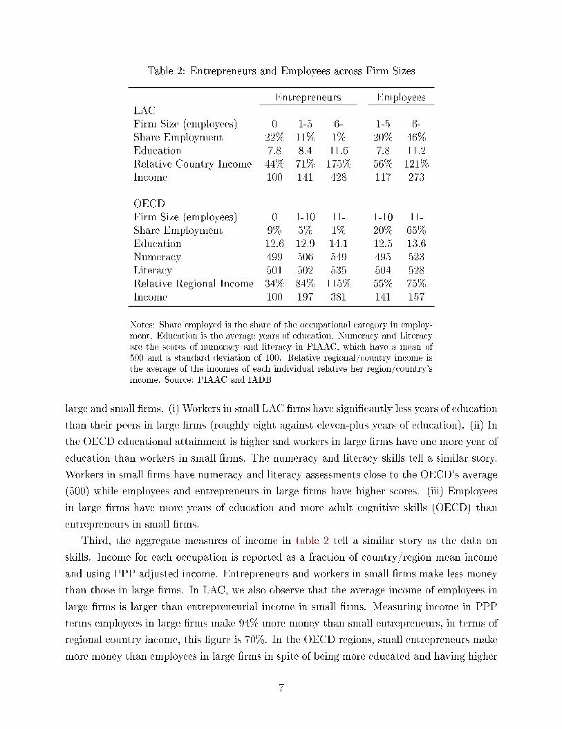
Table 2: Entrepreneurs and Employees across Firm Sizes

Entrepreneurs EmployeesLACFirm Size (employees) 0 1-5 6- 1-5 6-Share Employment 22% 11% 1% 20% 46%Education 7.8 8.4 11.6 7.8 11.2Relative Country Income 44% 71% 175% 56% 121%Income 100 141 428 117 273

OECDFirm Size (employees) 0 1-10 11- 1-10 11-Share Employment 9% 5% 1% 20% 65%Education 12.6 12.9 14.1 12.5 13.6Numeracy 499 506 549 495 523Literacy 501 502 535 504 528Relative Regional Income 34% 84% 115% 55% 75%Income 100 197 381 141 157

Notes: Share employed is the share of the occupational category in employ-ment. Education is the average years of education. Numeracy and Literacyare the scores of numeracy and literacy in PIAAC, which have a mean of500 and a standard deviation of 100. Relative regional/country income isthe average of the incomes of each individual relative her region/country'sincome. Source: PIAAC and IADB

large and small �rms. (i) Workers in small LAC �rms have signi�cantly less years of education

than their peers in large �rms (roughly eight against eleven-plus years of education). (ii) In

the OECD educational attainment is higher and workers in large �rms have one more year of

education than workers in small �rms. The numeracy and literacy skills tell a similar story.

Workers in small �rms have numeracy and literacy assessments close to the OECD's average

(500) while employees and entrepreneurs in large �rms have higher scores. (iii) Employees

in large �rms have more years of education and more adult cognitive skills (OECD) than

entrepreneurs in small �rms.

Third, the aggregate measures of income in table 2 tell a similar story as the data on

skills. Income for each occupation is reported as a fraction of country/region mean income

and using PPP adjusted income. Entrepreneurs and workers in small �rms make less money

than those in large �rms. In LAC, we also observe that the average income of employees in

large �rms is larger than entrepreneurial income in small �rms. Measuring income in PPP

terms employees in large �rms make 94% more money than small entrepreneurs, in terms of

regional country income, this �gure is 70%. In the OECD regions, small entrepreneurs make

more money than employees in large �rms in spite of being more educated and having higher

7

scores in tests of cognitive skills.

Fourth, conditional on �rm size, entrepreneurs make more money, have more years of

education and more numeracy and literacy ability than employees.

Skills and Occupational Choice

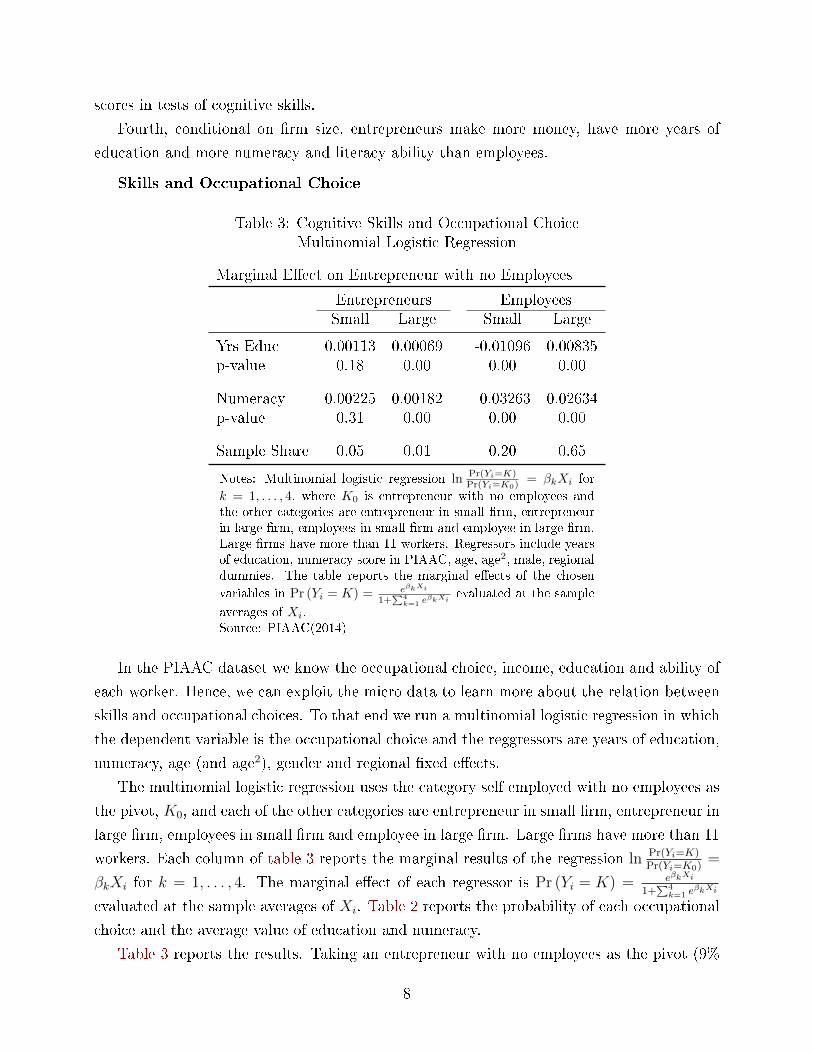
Table 3: Cognitive Skills and Occupational ChoiceMultinomial Logistic Regression

Marginal E�ect on Entrepreneur with no Employees

Entrepreneurs EmployeesSmall Large Small Large

Yrs Educ 0.00113 0.00069 -0.01096 0.00835p-value 0.18 0.00 0.00 0.00

Numeracy 0.00225 0.00182 -0.03263 0.02634p-value 0.31 0.00 0.00 0.00

Sample Share 0.05 0.01 0.20 0.65

Notes: Multinomial logistic regression ln Pr(Yi=K)Pr(Yi=K0) = βkXi for

k = 1, . . . , 4, where K0 is entrepreneur with no employees andthe other categories are entrepreneur in small �rm, entrepreneurin large �rm, employees in small �rm and employee in large �rm.Large �rms have more than 11 workers. Regressors include yearsof education, numeracy score in PIAAC, age, age2, male, regionaldummies. The table reports the marginal e�ects of the chosen

variables in Pr (Yi = K) = eβkXi

1+∑4k=1 eβkXi

evaluated at the sample

averages of Xi.Source: PIAAC(2014)

In the PIAAC dataset we know the occupational choice, income, education and ability of

each worker. Hence, we can exploit the micro data to learn more about the relation between

skills and occupational choices. To that end we run a multinomial logistic regression in which

the dependent variable is the occupational choice and the reggressors are years of education,

numeracy, age (and age2), gender and regional �xed e�ects.

The multinomial logistic regression uses the category self employed with no employees as

the pivot, K0, and each of the other categories are entrepreneur in small �rm, entrepreneur in

large �rm, employees in small �rm and employee in large �rm. Large �rms have more than 11

workers. Each column of table 3 reports the marginal results of the regression ln Pr(Yi=K)Pr(Yi=K0)

=

βkXi for k = 1, . . . , 4. The marginal e�ect of each regressor is Pr (Yi = K) = eβkXi

1+∑4k=1 e

βkXi

evaluated at the sample averages of Xi. Table 2 reports the probability of each occupational

choice and the average value of education and numeracy.

Table 3 reports the results. Taking an entrepreneur with no employees as the pivot (9%

8

of sample), increasing numeracy scores by one standard deviation (100 points) increases

the probability of being a small entrepreneur by 2.25%, a large e�ect considering that this

category captures 5% of the sample. For large entrepreneurs this marginal e�ect is 1.82%

relative to a 1% sample share of large entrepreneurs. The probability of being an employee

in a small �rm falls by 3.3% (relative to sample share of 20%) and the probability of being

an employee in a large �rm increases in 2.6% (relative to sample share of 65%). The residual

e�ect on the probability of being self-employed with no employees is -2.2%. The results using

years of education are qualitatively similar.

In summary, more years of education or more cognitive skills increase the probability of

working for a large �rm and of being an entrepreneur while they decrease the probability of

working for a small �rm or of being self-employed with no employees.

Mincer Regressions and Occupational Choice

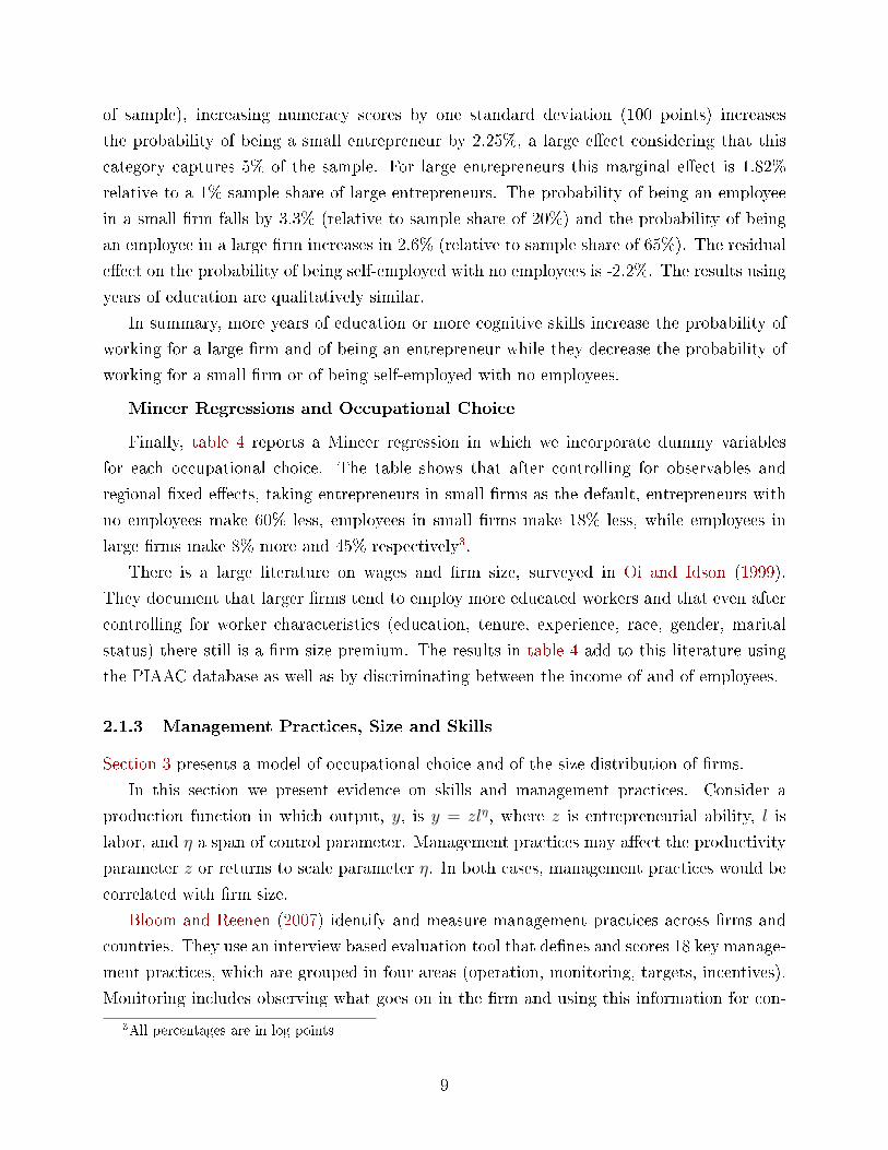
Finally, table 4 reports a Mincer regression in which we incorporate dummy variables

for each occupational choice. The table shows that after controlling for observables and

regional �xed e�ects, taking entrepreneurs in small �rms as the default, entrepreneurs with

no employees make 60% less, employees in small �rms make 18% less, while employees in

large �rms make 8% more and 45% respectively3.

There is a large literature on wages and �rm size, surveyed in Oi and Idson (1999).

They document that larger �rms tend to employ more educated workers and that even after

controlling for worker characteristics (education, tenure, experience, race, gender, marital

status) there still is a �rm size premium. The results in table 4 add to this literature using

the PIAAC database as well as by discriminating between the income of and of employees.

2.1.3 Management Practices, Size and Skills

Section 3 presents a model of occupational choice and of the size distribution of �rms.

In this section we present evidence on skills and management practices. Consider a

production function in which output, y, is y = zlη, where z is entrepreneurial ability, l is

labor, and η a span of control parameter. Management practices may a�ect the productivity

parameter z or returns to scale parameter η. In both cases, management practices would be

correlated with �rm size.

Bloom and Reenen (2007) identify and measure management practices across �rms and

countries. They use an interview based evaluation tool that de�nes and scores 18 key manage-

ment practices, which are grouped in four areas (operation, monitoring, targets, incentives).

Monitoring includes observing what goes on in the �rm and using this information for con-

3All percentages are in log points

9

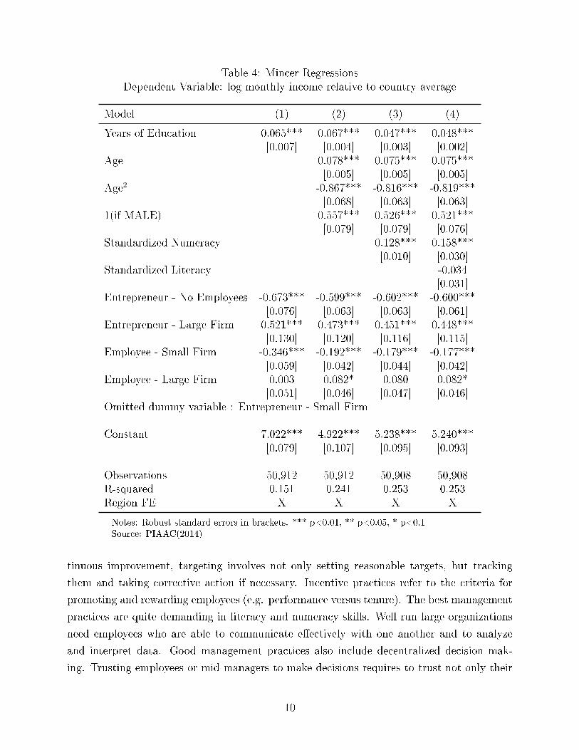
Table 4: Mincer RegressionsDependent Variable: log monthly income relative to country average

Model (1) (2) (3) (4)

Years of Education 0.065*** 0.067*** 0.047*** 0.048***[0.007] [0.004] [0.003] [0.002]

Age 0.078*** 0.075*** 0.075***[0.005] [0.005] [0.005]

Age2 -0.867*** -0.816*** -0.819***[0.068] [0.063] [0.063]

1(if MALE) 0.557*** 0.526*** 0.521***[0.079] [0.079] [0.076]

Standardized Numeracy 0.128*** 0.158***[0.010] [0.030]

Standardized Literacy -0.034[0.031]

Entrepreneur - No Employees -0.673*** -0.599*** -0.602*** -0.600***[0.076] [0.063] [0.063] [0.061]

Entrepreneur - Large Firm 0.521*** 0.473*** 0.451*** 0.448***[0.130] [0.120] [0.116] [0.115]

Employee - Small Firm -0.346*** -0.192*** -0.179*** -0.177***[0.059] [0.042] [0.044] [0.042]

Employee - Large Firm 0.003 0.082* 0.080 0.082*[0.051] [0.046] [0.047] [0.046]

Omitted dummy variable : Entrepreneur - Small Firm

Constant 7.022*** 4.922*** 5.238*** 5.240***[0.079] [0.107] [0.095] [0.093]

Observations 50,912 50,912 50,908 50,908R-squared 0.151 0.241 0.253 0.253Region FE X X X X

Notes: Robust standard errors in brackets. *** p<0.01, ** p<0.05, * p<0.1Source: PIAAC(2014)

tinuous improvement, targeting involves not only setting reasonable targets, but tracking

them and taking corrective action if necessary. Incentive practices refer to the criteria for

promoting and rewarding employees (e.g. performance versus tenure). The best management

practices are quite demanding in literacy and numeracy skills. Well run large organizations

need employees who are able to communicate e�ectively with one another and to analyze

and interpret data. Good management practices also include decentralized decision mak-

ing. Trusting employees or mid managers to make decisions requires to trust not only their

10

honesty (Bloom et al., 2012) but also their cognitive ability.

Figure 3, reproduced from Bloom et al. (2012), shows the distribution of management

scores across �rms in six countries. We observe that the distribution of management practices

in the US is better (stochastically dominate) than in developing countries such as Brazil,

China, and India. There are many factors that explain �bad� management practices such

as ownership (by the founder owner or the government), product market competition or

labor market regulations. For our purposes it is interesting to note that the human capital

of managers and workers, measured by the fraction of workers or managers with a college

degree or by the average real wage, is strongly correlated with management scores across

�rms (Bloom and Reenen (2007) and Bloom et al. (2012)). The fact that the education

of the workers, not only that of the managers, is correlated with high management scores

suggests that implementing good practices is easier in an environment with abundant human

capital. The management practices reported in �gure 3 are strongly correlated with �rm size.

Figure 3: Distribution of Management Scores Across Firms in Selected Countries

Source: Figure 2 in Bloom et al. (2012)

2.2 Mexico and United States

In this section we provide more detailed information on the distribution of cognitive abilities,

on the size distribution of �rms and on income distribution for Mexico and for the United

States.

11

2.2.1 Comparing the distribution of abilities in Mexico and the US

This section presents data on the distribution of abilities in Mexico. For comparison purposes

we also include data on advanced countries and on other Latin America countries.

We �rst present international measures of cognitive skills from Hanushek and Woessmann

(2009a) and regional measures of cognitive skills for Latin America. Between 1964 and

2003, twelve di�erent international tests of math, science, or reading were administered to

a voluntarily participating group of countries. The assessments were designed to identify

a common set of expected skills, which were then tested in the local language. It is easier

to do this in math and science than in reading, and a majority of the international testing

has focused on math and science. Hanushek and Woessmann (2009a) construct consistent

measures across tests that allow us to compare performance across countries even when they

did not each participate in a common assessment4. The scale of these assessments is calibrated

so that each age group and subject in the tests is normalized to the PISA standard of mean

500 and individual standard deviation of 100 across OECD countries. A very interesting

aspect of the Hanushek and Woessmann (2009a) paper is that they provide data on the

distribution of student achievement within countries. They calculate the share of students in

each country who reach at least basic skills as well as those who reach superior performance

levels. They use a test score of at least 400 in their transformed international scale�one

standard deviation below the OECD mean�as the threshold for basic literacy and numeracy

and a threshold of 600 points for superior performance5.

Table 5 reports data on cognitive abilities as measured by the test score in international

student achievement assessments in seven Latin American countries and an average for se-

lected advanced and East Asian countries. The cognitive skills of the average Latin American

student are below what is considered basic literacy in advanced countries. When we look

at the share of students that fail to achieve basic skills we observe that about half of the

students in Latin America do not attain basic skills in international tests while in advanced

countries this fraction of students is 8% and in East Asian countries only 4%. On the other

side of the distribution, in Latin America a tiny fraction of students show superior cognitive

skills, while in advanced countries almost 9% of students do.

4 The details of this construction as well as the data for all countries is in appendix B of their paper.5 The PISA 2003 science test uses the threshold of 400 points as the lowest bound for a basic level of

science literacy (Organization for Economic Co-operation and Development (2004), p. 292), and on the mathtest this corresponds to the middle of the level 1 range (358 to 420 test-score points), which denotes thatstudents can answer questions involving familiar contexts where all relevant information is present and thequestions are clearly de�ned. A score of 600 points is near the threshold of the level 5 range of performanceon the PISA 2003 math test, which denotes that students can develop and work with models for complexsituations, identifying constraints and specifying assumptions; they can re�ect on their answers and canformulate and communicate their interpretations and reasoning.

12

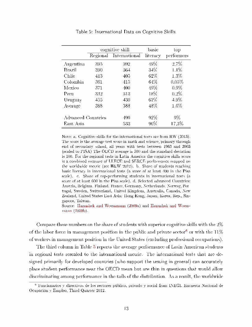
Table 5: International Data on Cognitive Skills.

cognitive skill basic topRegional International literacy performers

Argentina 395 392 49% 2.7%Brazil 390 364 34% 1.1%Chile 413 405 62% 1.3%Colombia 361 415 64% 0.05%Mexico 371 400 49% 0.9%Peru 332 313 18% 0.2%Uruguay 455 430 62% 4.9%Average 388 388 48% 1.6%

Advanced Countries 499 92% 9%East Asia 533 96% 17,3%

Note: a. Cognitive skills for the international tests are from HW (2013).The score is the average test score in math and science, primary throughend of secondary school, all years with tests between 1963 and 2003(scaled to PISA) The OECD average is 500 and the standard deviationis 100. For the regional tests in Latin America the cognitive skills scoreis a combined measure of LLECE and SERCE performance mapped onthe worldwide metric (see H&W 2012). b. Share of students reachingbasic literacy in international tests (a score of at least 400 in the Pisascale). c. Share of top-performing students in international tests (ascore of at least 600 in the Pisa scale). d. Selected advanced Countries:Austria, Belgium, Finland, France, Germany, Netherlands, Norway, Por-tugal, Sweden, Switzerland, United Kingdom, Australia, Canada, NewZealand, United States East Asia: Hong Kong, Japan, Korea, Rep., Sin-gapore, Taiwan.Source: Hanushek and Woessmann (2009a) and Hanushek and Woess-mann (2009b).

Compare these numbers on the share of students with superior cognitive skills with the 2%

of the labor force in management position in the public and private sector6 or with the 11%

of workers in management position in the United States (excluding professional occupations).

The third column in Table 5 reports the average performance of Latin American students

in regional tests rescaled to the international metric. The international tests that are de-

signed primarily for developed countries (who support the testing in general) can accurately

place student performance near the OECD mean but are thin in questions that would allow

discriminating among performance in the tails of the distribution. As a result, the worldwide

6 Funcionarios y directivos de los sectores público, privado y social from INEGI. Encuesta Nacional deOcupación y Empleo, Third Quarter 2012.

13

tests may be unable to distinguish reliably among varying levels of learning in the region of

Latin American students. The limitations of worldwide tests in discriminating at the level

of Latin American performance lead us to turn to two regional achievement tests speci�cally

designed for the Latin American countries. In 1997, the Latin American Laboratory for

the Assessment of Quality in Education Laboratorio Latinoamericano de Evaluacion de la

Calidad de la Educacion (LLECE) carried out the First International Comparative Study

in Language, Mathematics, and Associated Factors in the Third and Fourth Grades of Pri-

mary Education (Primer Estudio Internacional Comparativo) speci�cally designed to test

educational achievement in Latin American countries. In 2006, the Latin American bureau

of the UNESCO also conducted the Second Regional Comparative and Explanatory Study

(Segundo Estudio Regional Comparativo Explicativo, or SERCE). SERCE tested the perfor-

mance in math and reading of representative samples of students in third and sixth grades.

Column 3 in Table 5 reports the average of the country medians of these tests for the students

in fourth and sixth grade rescaled to the international metric computed by Hanushek and

Woessmann (2009b).

Figure 4 illustrates the statistics in table 5 with the test-scores of Mexican and US �fteen

year old students evaluated in the OECD Programme for International Student Assessment

(PISA) in 2009 for math and reading. Observe that the distribution of grades in the two

tests is similar within each country. We also see that about one half of Mexican students fall

bellow the 400 threshold for basic skills and that only a tiny fraction has scores above 600.

In addition to the di�erences in student achievement rates there are signi�cant di�erences

in educational attainment levels between Mexico and the United States. While in 2010, 87%

of the US population older than 25 years graduated from high school, in Mexico only a third

of the population of more than 25 years �nished high school7. For the younger cohorts the

numbers look better. In 2010, 70% of the population between 15 and 19 years completed at

least the basic education (5-15) in Mexico.

In conclusion, only a third of the Mexican population �nished high school and those who

did attend high school did very poorly in the tests designed to measure cognitive skills when

compared to the student population of advanced countries. About half of the students did not

attain the basic math and literacy skills of advanced countries and less than 1% of Mexican

students attained superior skills.

2.2.2 The Size Distribution of Firms and Informality

We now look at informality and the size distribution of �rms in Mexico. We follow Busso,

Fazio, and Levy (2012) in de�ning informality with reference to the observance of a particular

7Educación media superior

14

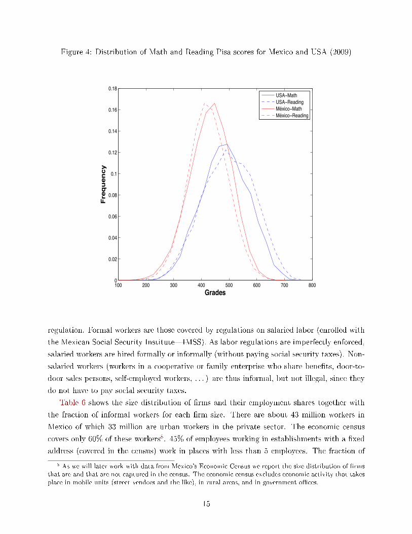
Figure 4: Distribution of Math and Reading Pisa scores for Mexico and USA (2009)

100 200 300 400 500 600 700 8000

0.02

0.04

0.06

0.08

0.1

0.12

0.14

0.16

0.18

Grades

Frequency

USA−MathUSA−ReadingMéxico−MathMéxico−Reading

regulation. Formal workers are those covered by regulations on salaried labor (enrolled with

the Mexican Social Security Institute�IMSS). As labor regulations are imperfectly enforced,

salaried workers are hired formally or informally (without paying social security taxes). Non-

salaried workers (workers in a cooperative or family enterprise who share bene�ts, door-to-

door sales persons, self-employed workers, . . . ) are thus informal, but not illegal, since they

do not have to pay social security taxes.

Table 6 shows the size distribution of �rms and their employment shares together with

the fraction of informal workers for each �rm size. There are about 43 million workers in

Mexico of which 33 million are urban workers in the private sector. The economic census

covers only 60% of these workers8. 45% of employees working in establishments with a �xed

address (covered in the census) work in places with less than 5 employees. The fraction of

8 As we will later work with data from Mexico's Economic Census we report the size distribution of �rmsthat are and that are not captured in the census. The economic census excludes economic activity that takesplace in mobile units (street vendors and the like), in rural areas, and in government o�ces.

15

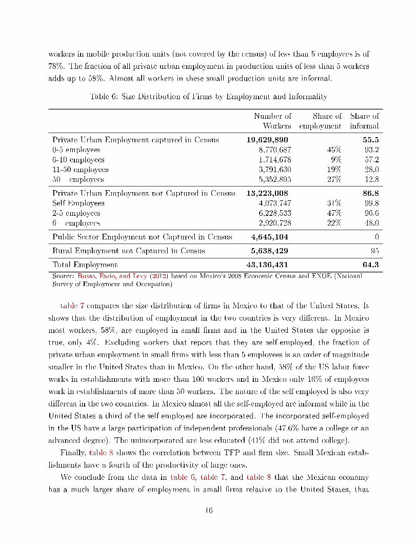
workers in mobile production units (not covered by the census) of less than 5 employees is of

78%. The fraction of all private urban employment in production units of less than 5 workers

adds up to 58%. Almost all workers in these small production units are informal.

Table 6: Size Distribution of Firms by Employment and Informality

Number of Share of Share ofWorkers employment informal

Private Urban Employment captured in Census 19,629,890 55.5

0-5 employees 8,770,687 45% 93.26-10 employees 1,714,678 9% 57.211-50 employees 3,791,630 19% 28.050+ employees 5,352,895 27% 12.8

Private Urban Employment not Captured in Census 13,223,008 86.8

Self Employees 4,073,747 31% 99.82-5 employees 6,228,533 47% 96.66+ employees 2,920,728 22% 48.0

Public Sector Employment not Captured in Census 4,645,104 0

Rural Employment not Captured in Census 5,638,429 95

Total Employment 43,136,431 64.3

Source: Busso, Fazio, and Levy (2012) based on Mexico's 2008 Economic Census and ENOE (NationalSurvey of Employment and Occupation)

table 7 compares the size distribution of �rms in Mexico to that of the United States. It

shows that the distribution of employment in the two countries is very di�erent. In Mexico

most workers, 58%, are employed in small �rms and in the United States the opposite is

true, only 4%. Excluding workers that report that they are self-employed, the fraction of

private urban employment in small �rms with less than 5 employees is an order of magnitude

smaller in the United States than in Mexico. On the other hand, 58% of the US labor force

works in establishments with more than 100 workers and in Mexico only 16% of employees

work in establishments of more than 50 workers. The nature of the self employed is also very

di�erent in the two countries. In Mexico almost all the self-employed are informal while in the

United States a third of the self employed are incorporated. The incorporated self-employed

in the US have a large participation of independent professionals (47.6% have a college or an

advanced degree). The unincorporated are less educated (41% did not attend college).

Finally, table 8 shows the correlation between TFP and �rm size. Small Mexican estab-

lishments have a fourth of the productivity of large ones.

We conclude from the data in table 6, table 7, and table 8 that the Mexican economy

has a much larger share of employment in small �rms relative to the United States, that

16

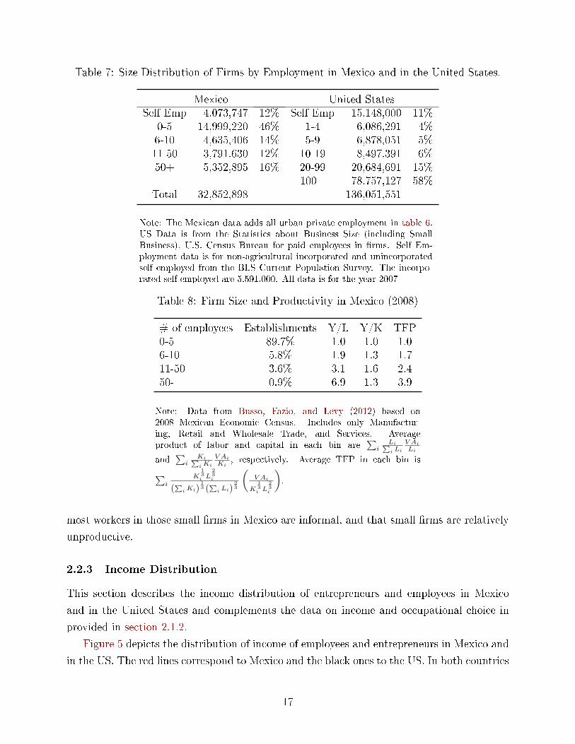
Table 7: Size Distribution of Firms by Employment in Mexico and in the United States.

Mexico United StatesSelf Emp 4,073,747 12% Self Emp 15,148,000 11%

0-5 14,999,220 46% 1-4 6,086,291 4%6-10 4,635,406 14% 5-9 6,878,051 5%11-50 3,791,630 12% 10-19 8,497,391 6%50+ 5,352,895 16% 20-99 20,684,691 15%

100+ 78,757,127 58%Total 32,852,898 136,051,551

Note: The Mexican data adds all urban private employment in table 6.US Data is from the Statistics about Business Size (including SmallBusiness), U.S. Census Bureau for paid employees in �rms. Self Em-ployment data is for non-agricultural incorporated and unincorporatedself employed from the BLS Current Population Survey. The incorpo-rated self employed are 5.591.000. All data is for the year 2007

Table 8: Firm Size and Productivity in Mexico (2008)

# of employees Establishments Y/L Y/K TFP0-5 89.7% 1.0 1.0 1.06-10 5.8% 1.9 1.3 1.711-50 3.6% 3.1 1.6 2.450- 0.9% 6.9 1.3 3.9

Note: Data from Busso, Fazio, and Levy (2012) based on2008 Mexican Economic Census. Includes only Manufactur-ing, Retail and Wholesale Trade, and Services. Averageproduct of labor and capital in each bin are

∑i

Li∑i Li

V AiLi

and∑

iKi∑iKi

V AiKi

, respectively. Average TFP in each bin is∑i

K13i L

23i

(∑iKi)

13 (

∑i Li)

23

(V Ai

K13i L

23i

).

most workers in those small �rms in Mexico are informal, and that small �rms are relatively

unproductive.

2.2.3 Income Distribution

This section describes the income distribution of entrepreneurs and employees in Mexico

and in the United States and complements the data on income and occupational choice in

provided in section 2.1.2.

Figure 5 depicts the distribution of income of employees and entrepreneurs in Mexico and

in the US. The red lines correspond to Mexico and the black ones to the US. In both countries

17

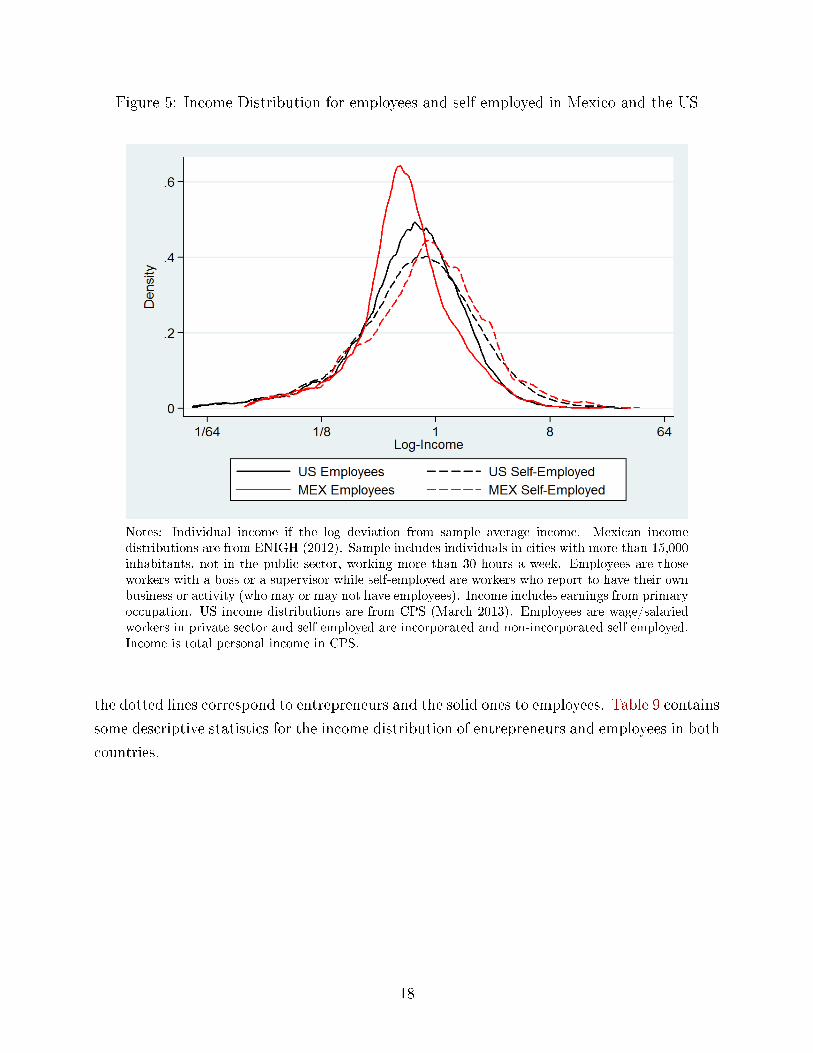
Figure 5: Income Distribution for employees and self employed in Mexico and the US

Notes: Individual income if the log deviation from sample average income. Mexican incomedistributions are from ENIGH (2012). Sample includes individuals in cities with more than 15,000inhabitants, not in the public sector, working more than 30 hours a week. Employees are thoseworkers with a boss or a supervisor while self-employed are workers who report to have their ownbusiness or activity (who may or may not have employees). Income includes earnings from primaryoccupation. US income distributions are from CPS (March 2013). Employees are wage/salariedworkers in private sector and self employed are incorporated and non-incorporated self employed.Income is total personal income in CPS.

the dotted lines correspond to entrepreneurs and the solid ones to employees. Table 9 contains

some descriptive statistics for the income distribution of entrepreneurs and employees in both

countries.

18

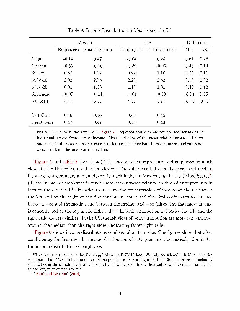
Table 9: Income Distribution in Mexico and the US

Mexico US Di�erence

Employees Entrepreneurs Employees Entrepreneurs Mex US

Mean -0.14 0.47 -0.04 0.23 0.61 0.26

Median -0.55 -0.10 -0.39 -0.26 0.46 0.13

St Dev 0.85 1.12 0.99 1.10 0.27 0.11

p90-p10 2.02 2.75 2.29 2.62 0.73 0.32

p75-p25 0.91 1.33 1.13 1.31 0.42 0.18

Skewness -0.07 -0.11 -0.64 -0.39 -0.04 0.25

Kurtosis 4.11 3.38 4.53 3.77 -0.73 -0.76

Left Gini 0.48 0.46 0.46 0.45

Right Gini 0.47 0.47 0.43 0.43

Notes: The data is the same as in �gure 5. reported statistics are for the log deviations of

individual income from average income. Mean is the log of the mean relative income. The left

and right Ginis measure income concentration near the median. Higher numbers indicate more

concentration of income near the median.

Figure 5 and table 9 show that (i) the income of entrepreneurs and employees is much

closer in the United States than in Mexico. The di�erence between the mean and median

income of entrepreneurs and employees is much higher in Mexico than in the United States9.

(ii) the income of employees is much more concentrated relative to that of entrepreneurs in

Mexico than in the US. In order to measure the concentration of income at the median at

the left and at the right of the distribution we computed the Gini coe�cients for income

between −∞ and the median and between the median and −∞ (�ipped so that most income

is concentrated at the top in the right tail)10. In both distribution in Mexico the left and the

right tails are very similar. In the US, the left sides of both distribution are more concentrated

around the median than the right sides, indicating fatter right tails.

Figure 6 shows income distributions conditional on �rm size. The �gures show that after

conditioning for �rm size the income distribution of entrepreneurs stochastically dominates

the income distribution of employees.

9This result is sensitive to the �lters applied to the ENIGH data. We only considered individuals in citieswith more than 15,000 inhabitants, not in the public sector, working more than 30 hours a week. Includingsmall cities in the sample (rural areas) or part time workers shifts the distribution of entrepreneurial incometo the left, reversing this result.

10 Fiori and Beltrami (2014)

19

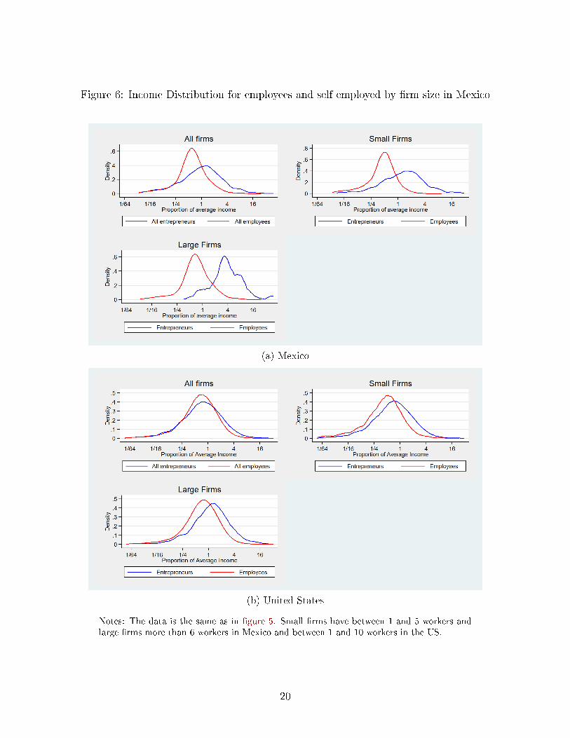
Figure 6: Income Distribution for employees and self employed by �rm size in Mexico

(a) Mexico

(b) United States

Notes: The data is the same as in �gure 5. Small �rms have between 1 and 5 workers andlarge �rms more than 6 workers in Mexico and between 1 and 10 workers in the US.

20

3 The Model

We now write a model of occupational choice, the size distribution of �rms and informality.

The model endogenously determines who becomes an entrepreneur or a wage-employee, the

size distribution of �rms, the income distribution of workers and entrepreneurs, and the

fraction of formal workers in each �rm. Several key assumptions play an important role in

our model. (i) As in Lucas (1978) agents di�er in their entrepreneurial talent and the size

distribution of �rms depends on the distribution of this type of ability in the population.

(ii) We introduce a second source of heterogeneity among agents that is their ability as

wage employees. We have in mind that individuals di�er in their ability to work in teams,

understand and respond to instructions, be punctual, presentable and courteous, etc. The

basic extension of the Lucas (1978) model in this dimension is outlined in Jovanovic (1994).

(iii) Finally, we assume that tax enforcement is imperfect and that �rms are audited with

a probability that is increasing in the size of the �rm (see Áureo De Paula and Scheinkman

(2011) and Bigio and Zilberman (2011)).

The economy is populated by a continuum of agents with mass 1. Each household is

endowed with an ability bundle z ≡ (zei , zwi ) of entrepreneurial talent, zei , and e�ciency

units of labor as wage employees, zwi . Talents are jointly distributed according to the prob-

ability density function Φ (zei , zwi ) on the positive real numbers, which we assume to be a

bivariate lognormal distribution, ln z ∼ N (λz,Σz) where λz and Σz are the mean and the

variance-covariance matrix of the joint distribution of entrepreneurial abilities and abilities

as workers.11

Let Li =∫ li

0zwijdj be the e�ciency units of labor employed by �rm i, where zwij is the

ability of a worker of type j hired by �rm i. As each worker supplies a unit of time, e�ective

labor is given by the sum of the working abilities hired by each entrepreneur. As worker

types are perfect substitutes, the number of employees (bodies), li, hired by each �rm i is

undetermined. An entrepreneurs with talent bundle zi produces with the technology

Yi = zeiLηi , (1)

where 0 < η < 1.

Agents are endowed with a unit of time and, as in Roy (1951), will self-select comparing

11One possible interpretation of this formulation is to think that agents' abilities as workers and en-trepreneurs (in logs) are a linear transformation of the cognitive abilities measured in the assessment testsplus some random ability shock, so that ln z = T A+ε. where A ∈ R2, ε is a bivariate normal random variableand T is the measured cognitive skill in student assessment test.

21

their earnings as employees, wzwi , with their pro�ts as entrepreneurs,

π (zei , w) = (1− η)ηη

1−η zei1

1−ηw−η

1−η . (2)

The set of entrepreneurs A will be the set of agents that are better-o� as entrepreneurs than

working as employees.

A (w) = {(zei , zwi ) | π (zei , w) ≥ wzwi } (3)

For the technology in equation (1) we can de�ne a critical

z̄wi (zei , w) = (1− η)ηη

1−η

(zeiw

) 11−η

(4)

such that for each zei and w an agent becomes an entrepreneur if, and only if, zwi < z̄wi (zei , w).

Figure 7 shows z̄wi (zei , w) as a function of zei for two di�erent values of wages. The interaction

between the level of wages and the distribution of abilities determines income distribution

and occupational choice. In particular, it is possible to have many low ability entrepreneurs.

In the general equilibrium, wages equate the supply and the demand for labor at the

optimal occupational choice. Aggregating the optimal labor choice of each �rm, (ηzei /w)1

1−η ,

in the set A (w) we obtain the economy's demand for labor.

LD (w) =( ηw

) 11−η∫ ∞

0

zei1

1−η

(∫ z̄wi (zei ,w)

0

Φ(zwi |zei )dzhi

)Φ(zei )dz

ei , (5)

where Φ(zhi |zei ) is the density of zwi conditional on zei and Φ(zei ) is the marginal density of

zei . The �rst term in equation (5) captures the e�ect of wages on labor demand through

the intensive margin and the upper limit inner integral the e�ect of wages on labor demand

through the extensive margin. Increases in wages reduce the labor demand of each �rm and

shift the critical z̄ri in �gure 7 downwards reducing the number of �rms.

Analogously, the labor supply is the aggregate ability of agents that become workers, i.e.,

LS (w) =

∫ ∞0

(∫ ∞z̄wi (zei ,w)

zhi Φ(zhi |zei

)dzhi

)Φ(zei )dz

ei (6)

The labor supply is increasing in w as higher wages induce more agents to become employees.

The equilibrium wage, w∗, solves LD(w∗) = LS(w∗) and knowing the equilibrium wage

22

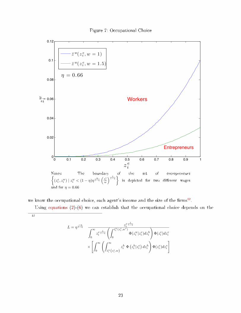
Figure 7: Occupational Choice

0 0.1 0.2 0.3 0.4 0.5 0.6 0.7 0.8 0.9 10

0.02

0.04

0.06

0.08

0.1

0.12

z ei

zw i

Entrepreneurs

Workers

η = 0.66

z̄ w(z ei , w = 1)

z̄ w(z ei , w = 1.5)

Notes: The boundary of the set of entrepreneurs{(zei , z

wi ) | zwi < (1− η)η

η1−η

(zeiw

) 11−η}

is depicted for two di�erent wages

and for η = 0.66

we know the occupational choice, each agent's income and the size of the �rms12.

Using equations (2)-(6) we can establish that the occupational choice depends on the

12

L = η−η1−η

zei1

1−η∫ ∞0

zei1

1−η

(∫ z̄wi (zei ,w∗)

0

Φ(zwi |zei )dzhi

)Φ(zei )dzei

×

[∫ ∞0

(∫ ∞z̄wi (zei ,w)

zhi Φ(zhi |zei

)dzhi

)Φ(zei )dzei

]

23

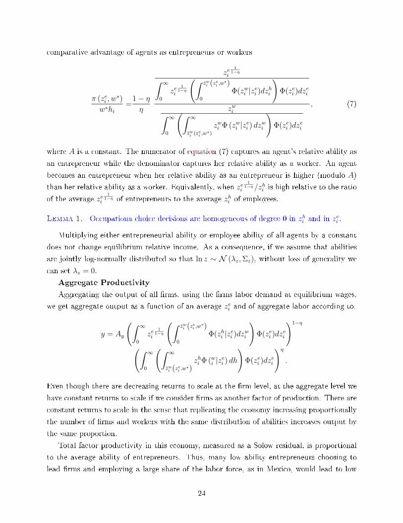
comparative advantage of agents as entrepreneurs or workers

π (zei , w∗)

w∗hi=

1− ηη

zei1

1−η∫ ∞0

zei1

1−η

(∫ z̄wi (zei ,w∗)

0

Φ(zwi |zei )dzhi

)Φ(zei )dz

ei

zwi∫ ∞0

(∫ ∞z̄wi (zei ,w

∗)

zwi Φ (zwi |zei ) dzwi

)Φ(zei )dz

ei

, (7)

where A is a constant. The numerator of equation (7) captures an agent's relative ability as

an entrepreneur while the denominator captures her relative ability as a worker. An agent

becomes an entrepreneur when her relative ability as an entrepreneur is higher (modulo A)

than her relative ability as a worker. Equivalently, when zei1

1−η /zhi is high relative to the ratio

of the average zei1

1−η of entrepreneurs to the average zhi of employees.

Lemma 1. Occupationa choice decisions are homogeneous of degree 0 in zhi and in zei .

Multiplying either entrepreneurial ability or employee ability of all agents by a constant

does not change equilibrium relative income. As a consequence, if we assume that abilities

are jointly log-normally distributed so that ln z ∼ N (λz,Σz), without loss of generality we

can set λz = 0.

Aggregate Productivity

Aggregating the output of all �rms, using the �rms labor demand at equilibrium wages,

we get aggregate output as a function of an average zei and of aggregate labor according to.

y = Ay

(∫ ∞0

zei1

1−η

(∫ z̄wi (zei ,w∗)

0

Φ(zhi |zei )dzwi

)Φ(zei )dz

ei

)1−η

(∫ ∞0

(∫ ∞z̄wi (zei ,w∗)

zhi Φ (wi |zei ) dh

)Φ(zei )dz

ei

)η

.

Even though there are decreasing returns to scale at the �rm level, at the aggregate level we

have constant returns to scale if we consider �rms as another factor of production. There are

constant returns to scale in the sense that replicating the economy increasing proportionally

the number of �rms and workers with the same distribution of abilities increases output by

the same proportion.

Total factor productivity in this economy, measured as a Solow residual, is proportional

to the average ability of entrepreneurs. Thus, many low ability entrepreneurs choosing to

lead �rms and employing a large share of the labor force, as in Mexico, would lead to low

24

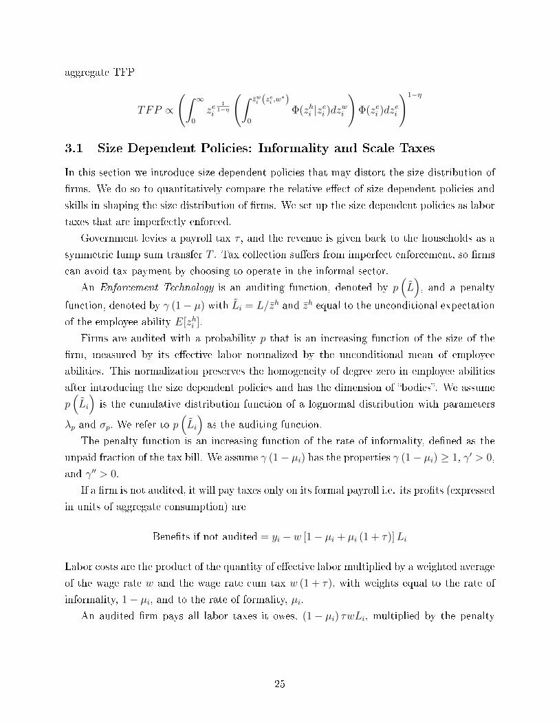
aggregate TFP

TFP ∝

(∫ ∞0

zei1

1−η

(∫ z̄wi (zei ,w∗)

0

Φ(zhi |zei )dzwi

)Φ(zei )dz

ei

)1−η

3.1 Size Dependent Policies: Informality and Scale Taxes

In this section we introduce size dependent policies that may distort the size distribution of

�rms. We do so to quantitatively compare the relative e�ect of size dependent policies and

skills in shaping the size distribution of �rms. We set up the size dependent policies as labor

taxes that are imperfectly enforced.

Government levies a payroll tax τ , and the revenue is given back to the households as a

symmetric lump sum transfer T . Tax collection su�ers from imperfect enforcement, so �rms

can avoid tax payment by choosing to operate in the informal sector.

An Enforcement Technology is an auditing function, denoted by p(L̃), and a penalty

function, denoted by γ (1− µ) with L̃i = L/z̄h and z̄h equal to the unconditional expectation

of the employee ability E[zhi ].

Firms are audited with a probability p that is an increasing function of the size of the

�rm, measured by its e�ective labor normalized by the unconditional mean of employee

abilities. This normalization preserves the homogeneity of degree zero in employee abilities

after introducing the size dependent policies and has the dimension of �bodies�. We assume

p(L̃i

)is the cumulative distribution function of a lognormal distribution with parameters

λp and σp. We refer to p(L̃i

)as the auditing function.

The penalty function is an increasing function of the rate of informality, de�ned as the

unpaid fraction of the tax bill. We assume γ (1− µi) has the properties γ (1− µi) ≥ 1, γ′ > 0,

and γ′′ > 0.

If a �rm is not audited, it will pay taxes only on its formal payroll i.e. its pro�ts (expressed

in units of aggregate consumption) are

Bene�ts if not audited = yi − w [1− µi + µi (1 + τ)]Li

Labor costs are the product of the quantity of e�ective labor multiplied by a weighted average

of the wage rate w and the wage rate cum tax w (1 + τ), with weights equal to the rate of

informality, 1− µi, and to the rate of formality, µi.

An audited �rm pays all labor taxes it owes, (1− µi) τwLi, multiplied by the penalty

25

function over its tax liability, γ (1− µi). Pro�ts for audited �rms are

Bene�ts if audited = yi − [(1− µi) (1 + γ (1− µi) τ) + µi (1 + τ)]wLi

Firms choose the fraction of formal workers µi and the level of employment Li to maximize

expected pro�ts

E[πi (zei , w)] = zeiL

η − (1 + µτ + p(1− µ)γτ)wL,

where p is a function of L̃i and γ is a function of µ.

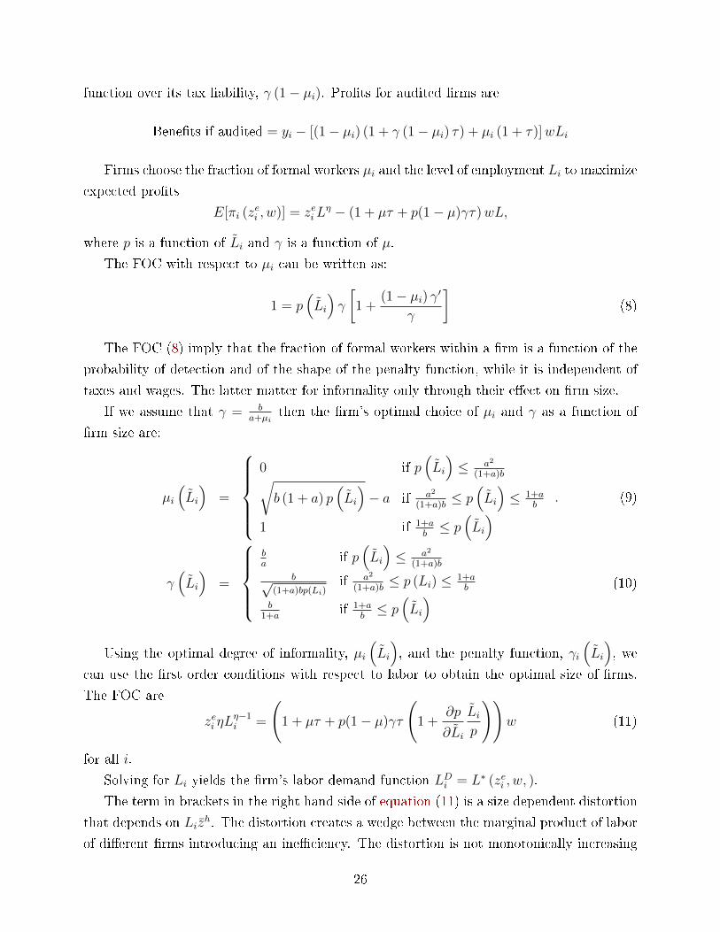
The FOC with respect to µi can be written as:

1 = p(L̃i

)γ

[1 +

(1− µi) γ′

γ

](8)

The FOC (8) imply that the fraction of formal workers within a �rm is a function of the

probability of detection and of the shape of the penalty function, while it is independent of

taxes and wages. The latter matter for informality only through their e�ect on �rm size.

If we assume that γ = ba+µi

then the �rm's optimal choice of µi and γ as a function of

�rm size are:

µi

(L̃i

)=

0 if p

(L̃i

)≤ a2

(1+a)b√b (1 + a) p

(L̃i

)− a if a2

(1+a)b≤ p

(L̃i

)≤ 1+a

b

1 if 1+ab≤ p

(L̃i

) . (9)

γ(L̃i

)=

ba

if p(L̃i

)≤ a2

(1+a)b

b√(1+a)bp(Li)

if a2

(1+a)b≤ p (Li) ≤ 1+a

b

b1+a

if 1+ab≤ p

(L̃i

) (10)

Using the optimal degree of informality, µi(L̃i

), and the penalty function, γi

(L̃i

), we

can use the �rst order conditions with respect to labor to obtain the optimal size of �rms.

The FOC are

zei ηLη−1i =

(1 + µτ + p(1− µ)γτ

(1 +

∂p

∂L̃i

L̃ip

))w (11)

for all i.

Solving for Li yields the �rm's labor demand function LDi = L∗ (zei , w, ).

The term in brackets in the right hand side of equation (11) is a size dependent distortion

that depends on Liz̄h. The distortion creates a wedge between the marginal product of labor

of di�erent �rms introducing an ine�ciency. The distortion is not monotonically increasing

26

in Li since the elasticity of the auditing function is not.

The optimal degree of informality in equation (9) implies that in equilibrium some �rms

will be informal (µ = 0), some �rms will be semi-formal 0 < µ < 1, and some �rms will

be formal µ = 1. Small informal �rms will set their marginal product close to w as the

auditing probability and its derivative are very small for very small �rms. On the other

hand, formal �rms will set their marginal product close to w(1 + τ) as for large �rms the

auditing probability is close to one and its derivative close to zero. Thus, the marginal

product of large �rms will be larger than the marginal product of small �rms.

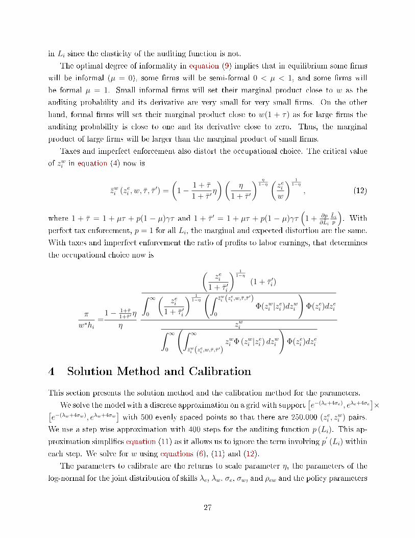
Taxes and imperfect enforcement also distort the occupational choice. The critical value

of zwi in equation (4) now is

z̄wi (zei , w, τ̄ , τ̄′) =

(1− 1 + τ̄

1 + τ̄ ′η

)(η

1 + τ̄ ′

) η1−η(zeiw

) 11−η

, (12)

where 1 + τ̄ = 1 + µτ + p(1 − µ)γτ and 1 + τ̄ ′ = 1 + µτ + p(1 − µ)γτ(

1 + ∂p

∂L̃i

L̃ip

). With

perfect tax enforcement, p = 1 for all Li, the marginal and expected distortion are the same.

With taxes and imperfect enforcement the ratio of pro�ts to labor earnings, that determines

the occupational choice now is

π

w∗hi=

1− 1+τ̄1+τ̄ ′

η

η

(zei

1 + τ̄ ′i

) 11−η

(1 + τ̄ ′i)∫ ∞0

(zei

1 + τ̄ ′i

) 11−η(∫ z̄wi (zei ,w,τ̄ ,τ̄ ′)

0

Φ(zwi |zei )dzwi

)Φ(zei )dz

ei

zwi∫ ∞0

(∫ ∞z̄wi (zei ,w,τ̄ ,τ̄ ′)

zwi Φ (zwi |zei ) dzwi

)Φ(zei )dz

ei

4 Solution Method and Calibration

This section presents the solution method and the calibration method for the parameters.

We solve the model with a discrete approximation on a grid with support[e−(λe+4σe), eλe+4σe

]×[

e−(λw+4σw), eλw+4σw]with 500 evenly spaced points so that there are 250.000 (zei , z

wi ) pairs.

We use a step wise approximation with 400 steps for the auditing function p (Li). This ap-

proximation simpli�es equation (11) as it allows us to ignore the term involving p′(Li) within

each step. We solve for w using equations (6), (11) and (12).

The parameters to calibrate are the returns to scale parameter η, the parameters of the

log-normal for the joint distribution of skills λe, λw, σe, σw, and ρew and the policy parameters

27

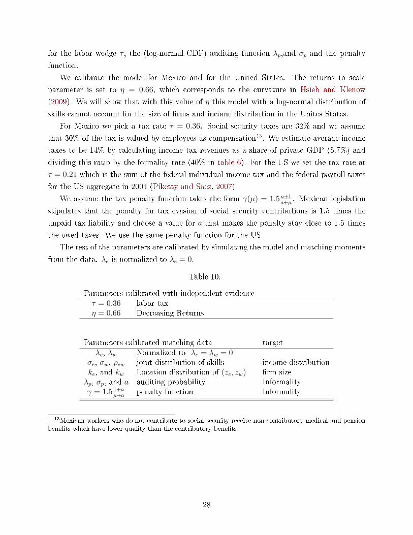
for the labor wedge τ , the (log-normal CDF) auditing function λp,and σp and the penalty

function.

We calibrate the model for Mexico and for the United States. The returns to scale

parameter is set to η = 0.66, which corresponds to the curvature in Hsieh and Klenow

(2009). We will show that with this value of η this model with a log-normal distribution of

skills cannot account for the size of �rms and income distribution in the Unites States.

For Mexico we pick a tax rate τ = 0.36. Social security taxes are 32% and we assume

that 30% of the tax is valued by employees as compensation13. We estimate average income

taxes to be 14% by calculating income tax revenues as a share of private GDP (5.7%) and

dividing this ratio by the formality rate (40% in table 6). For the US we set the tax rate at

τ = 0.21 which is the sum of the federal individual income tax and the federal payroll taxes

for the US aggregate in 2004 (Piketty and Saez, 2007)

We assume the tax penalty function takes the form γ(µ) = 1.5 a+1a+µ

. Mexican legislation

stipulates that the penalty for tax evasion of social security contributions is 1.5 times the

unpaid tax liability and choose a value for a that makes the penalty stay close to 1.5 times

the owed taxes. We use the same penalty function for the US.

The rest of the parameters are calibrated by simulating the model and matching moments

from the data. λe is normalized to λe = 0.

Table 10:

Parameters calibrated with independent evidenceτ = 0.36 labor taxη = 0.66 Decreasing Returns

Parameters calibrated matching data targetλe, λw Normalized to λe = λw = 0

σe, σw, ρew joint distribution of skills income distributionke, and kw Location distribution of (ze, zw) �rm sizeλp, σp, and a auditing probability Informalityγ = 1.5 1+a

µ+apenalty function Informality

13Mexican workers who do not contribute to social security receive non-contributory medical and pensionbene�ts which have lower quality than the contributory bene�ts

28

5 Results and Comparative Statics

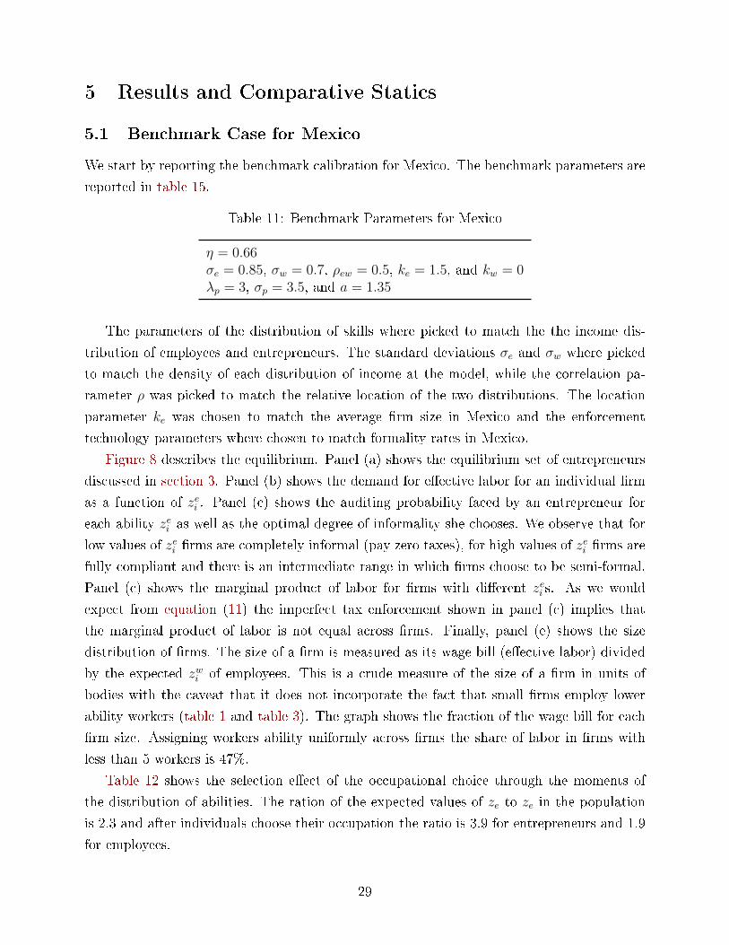
5.1 Benchmark Case for Mexico

We start by reporting the benchmark calibration for Mexico. The benchmark parameters are

reported in table 15.

Table 11: Benchmark Parameters for Mexico

η = 0.66σe = 0.85, σw = 0.7, ρew = 0.5, ke = 1.5, and kw = 0λp = 3, σp = 3.5, and a = 1.35

The parameters of the distribution of skills where picked to match the the income dis-

tribution of employees and entrepreneurs. The standard deviations σe and σw where picked

to match the density of each distribution of income at the model, while the correlation pa-

rameter ρ was picked to match the relative location of the two distributions. The location

parameter ke was chosen to match the average �rm size in Mexico and the enforcement

technology parameters where chosen to match formality rates in Mexico.

Figure 8 describes the equilibrium. Panel (a) shows the equilibrium set of entrepreneurs

discussed in section 3. Panel (b) shows the demand for e�ective labor for an individual �rm

as a function of zei . Panel (c) shows the auditing probability faced by an entrepreneur for

each ability zei as well as the optimal degree of informality she chooses. We observe that for

low values of zei �rms are completely informal (pay zero taxes), for high values of zei �rms are

fully compliant and there is an intermediate range in which �rms choose to be semi-formal.

Panel (c) shows the marginal product of labor for �rms with di�erent zei s. As we would

expect from equation (11) the imperfect tax enforcement shown in panel (c) implies that

the marginal product of labor is not equal across �rms. Finally, panel (e) shows the size

distribution of �rms. The size of a �rm is measured as its wage bill (e�ective labor) divided

by the expected zwi of employees. This is a crude measure of the size of a �rm in units of

bodies with the caveat that it does not incorporate the fact that small �rms employ lower

ability workers (table 1 and table 3). The graph shows the fraction of the wage bill for each

�rm size. Assigning workers ability uniformly across �rms the share of labor in �rms with

less than 5 workers is 47%.

Table 12 shows the selection e�ect of the occupational choice through the moments of

the distribution of abilities. The ration of the expected values of ze to ze in the population

is 2.3 and after individuals choose their occupation the ratio is 3.9 for entrepreneurs and 1.9

for employees.

29

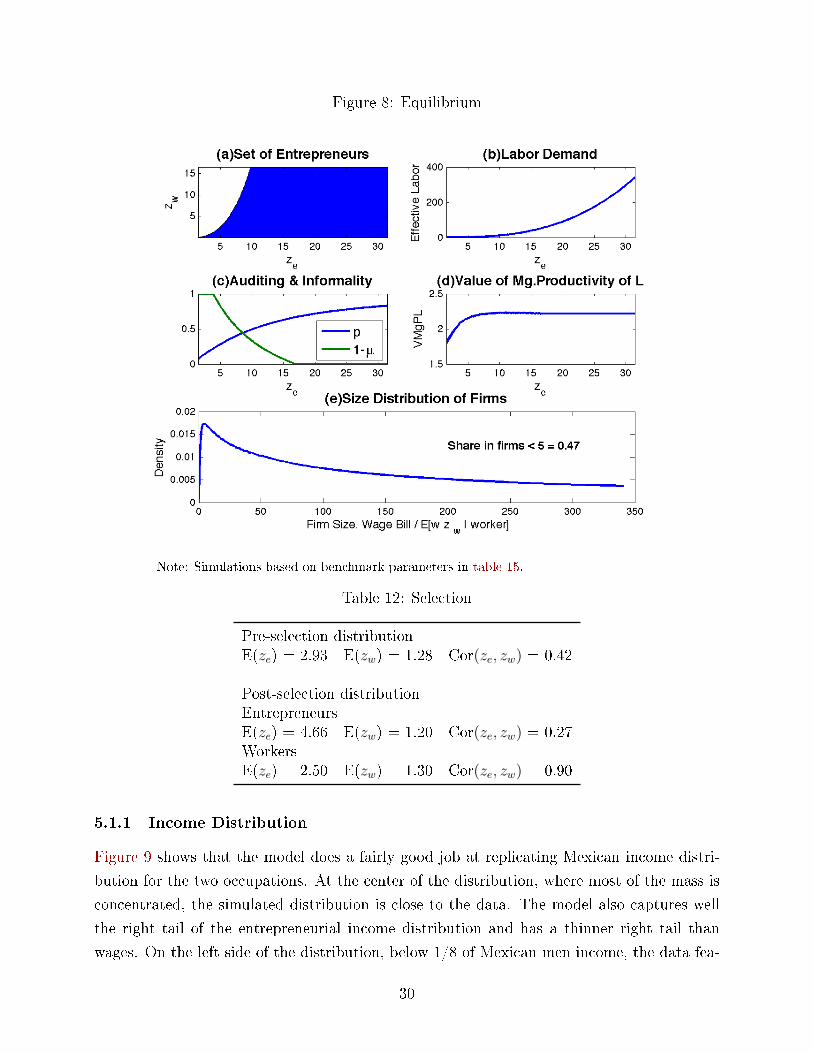
Figure 8: Equilibrium

Note: Simulations based on benchmark parameters in table 15.

Table 12: Selection

Pre-selection distributionE(ze) = 2.93 E(zw) = 1.28 Cor(ze, zw) = 0.42

Post-selection distributionEntrepreneursE(ze) = 4.66 E(zw) = 1.20 Cor(ze, zw) = 0.27WorkersE(ze) = 2.50 E(zw) = 1.30 Cor(ze, zw) = 0.90

5.1.1 Income Distribution

Figure 9 shows that the model does a fairly good job at replicating Mexican income distri-

bution for the two occupations. At the center of the distribution, where most of the mass is

concentrated, the simulated distribution is close to the data. The model also captures well

the right tail of the entrepreneurial income distribution and has a thinner right tail than

wages. On the left side of the distribution, below 1/8 of Mexican men income, the data fea-

30

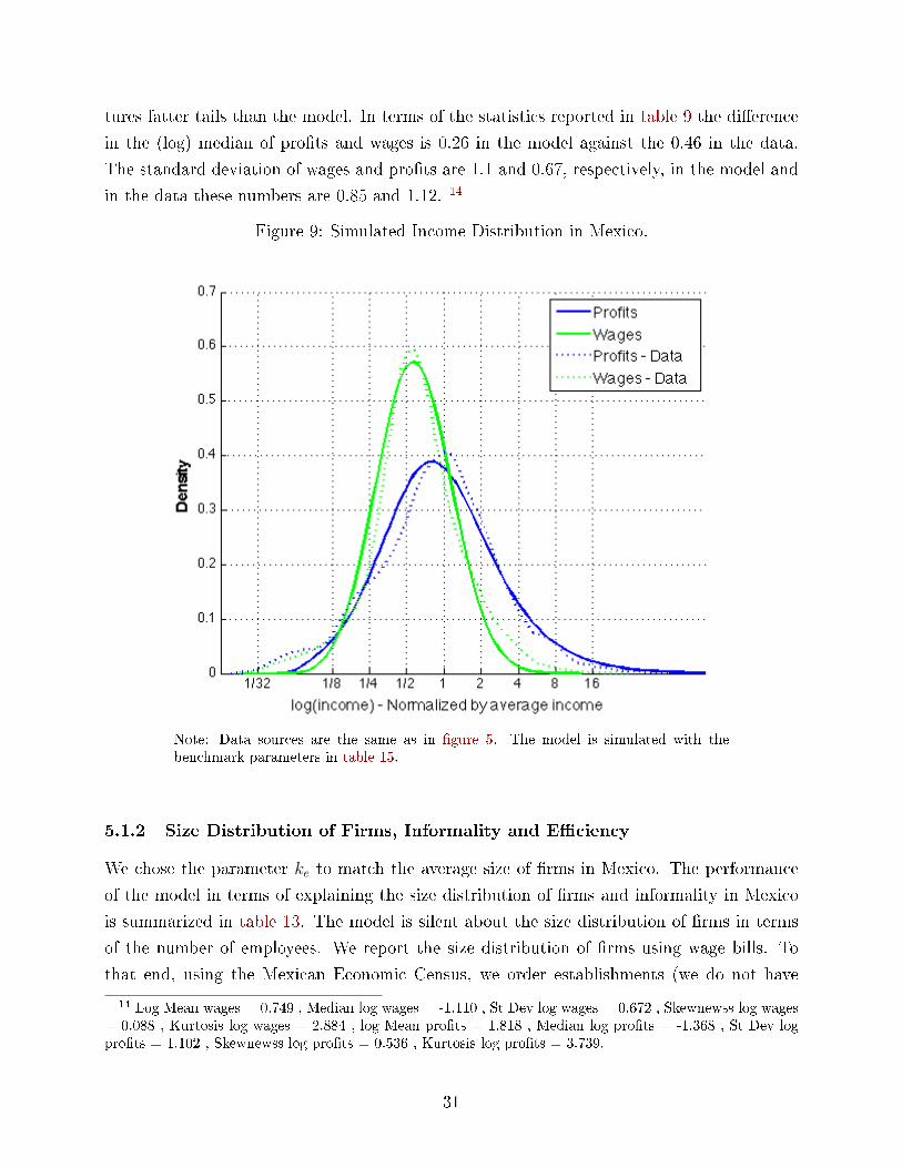
tures fatter tails than the model. In terms of the statistics reported in table 9 the di�erence

in the (log) median of pro�ts and wages is 0.26 in the model against the 0.46 in the data.

The standard deviation of wages and pro�ts are 1.1 and 0.67, respectively, in the model and

in the data these numbers are 0.85 and 1.12. 14

Figure 9: Simulated Income Distribution in Mexico.

Note: Data sources are the same as in �gure 5. The model is simulated with thebenchmark parameters in table 15.

5.1.2 Size Distribution of Firms, Informality and E�ciency

We chose the parameter ke to match the average size of �rms in Mexico. The performance

of the model in terms of explaining the size distribution of �rms and informality in Mexico

is summarized in table 13. The model is silent about the size distribution of �rms in terms

of the number of employees. We report the size distribution of �rms using wage bills. To

that end, using the Mexican Economic Census, we order establishments (we do not have

14 Log Mean wages = 0.749 , Median log wages = -1.110 , St Dev log wages = 0.672 , Skewnewss log wages= 0.088 , Kurtosis log wages = 2.884 , log Mean pro�ts = 1.818 , Median log pro�ts = -1.368 , St Dev logpro�ts = 1.102 , Skewnewss log pro�ts = 0.536 , Kurtosis log pro�ts = 3.739.

31

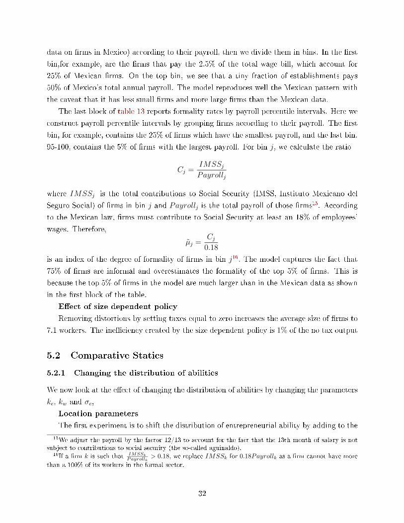
data on �rms in Mexico) according to their payroll, then we divide them in bins. In the �rst

bin,for example, are the �rms that pay the 2.5% of the total wage bill, which account for

25% of Mexican �rms. On the top bin, we see that a tiny fraction of establishments pays

50% of Mexico's total annual payroll. The model reproduces well the Mexican pattern with

the caveat that it has less small �rms and more large �rms than the Mexican data.

The last block of table 13 reports formality rates by payroll percentile intervals. Here we

construct payroll percentile intervals by grouping �rms according to their payroll. The �rst

bin, for example, contains the 25% of �rms which have the smallest payroll, and the last bin,

95-100, contains the 5% of �rms with the largest payroll. For bin j, we calculate the ratio

Cj =IMSSjPayrollj

where IMSSj is the total contributions to Social Security (IMSS, Instituto Mexicano del

Seguro Social) of �rms in bin j and Payrollj is the total payroll of those �rms15. According

to the Mexican law, �rms must contribute to Social Security at least an 18% of employees'

wages. Therefore,

µ̃j =Cj

0.18

is an index of the degree of formality of �rms in bin j16. The model captures the fact that

75% of �rms are informal and overestimates the formality of the top 5% of �rms. This is

because the top 5% of �rms in the model are much larger than in the Mexican data as shown

in the �rst block of the table.

E�ect of size dependent policy

Removing distortions by setting taxes equal to zero increases the average size of �rms to

7.1 workers. The ine�ciency created by the size dependent policy is 1% of the no tax output

5.2 Comparative Statics

5.2.1 Changing the distribution of abilities

We now look at the e�ect of changing the distribution of abilities by changing the parameters

ke, kw and σe,

Location parameters

The �rst experiment is to shift the distribution of entrepreneurial ability by adding to the

15We adjust the payroll by the factor 12/13 to account for the fact that the 13th month of salary is notsubject to contributions to social security (the so-called aguinaldo).

16If a �rm k is such that IMSSkPayrollk

> 0.18, we replace IMSSk for 0.18Payrollk as a �rm cannot have more

than a 100% of its workers in the formal sector.

32

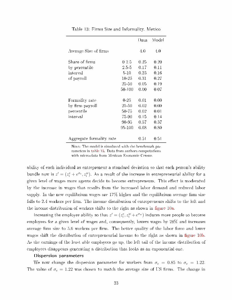
Table 13: Firms Size and Informality. Mexico

Data Model

Average Size of �rms 4.0 4.0

Share of �rms 0-2.5 0.25 0.20by percentile 2.5-5 0.17 0.11interval 5-10 0.23 0.16of payroll 10-25 0.31 0.27

25-50 0.05 0.1950-100 0.00 0.07

Formality rate 0-25 0.01 0.00by �rm payroll 25-50 0.02 0.00percentile 50-75 0.02 0.01interval 75-90 0.15 0.14

90-95 0.57 0.3795-100 0.68 0.80

Aggregate formality rate 0.51 0.51

Note: The model is simulated with the benchmark pa-rameters in table 15. Data from authors computationswith micro-data from Mexican Economic Census

ability of each individual as entrepreneur a standard deviation so that each person's ability

bundle now is z′ = (zei + eσe , zwi ). As a result of the increase in entrepreneurial ability for a

given level of wages more agents decide to become entrepreneurs. This e�ect is moderated

by the increase in wages that results from the increased labor demand and reduced labor

supply. In the new equilibrium wages are 17% higher and the equilibrium average �rm size

falls to 2.4 workers per �rm. The income distribution of entrepreneurs shifts to the left and

the income distribution of workers shifts to the right as shown in �gure 10a.

Increasing the employee ability so that z′ = (zei , zwi + eσw) induces more people to become

employees for a given level of wages and, consequently, lowers wages by 28% and increases

average �rm size to 5.6 workers per �rm. The better quality of the labor force and lower

wages shift the distribution of entrepreneurial income to the right as shown in �gure 10b.

As the earnings of the least able employees go up, the left tail of the income distribution of

employees disappears generating a distribution that looks as an exponential one.

Dispersion parameters

We now change the dispersion parameter for workers from σe = 0.85 to σe = 1.22.

The value of σe = 1.22 was chosen to match the average size of US �rms. The change in

33

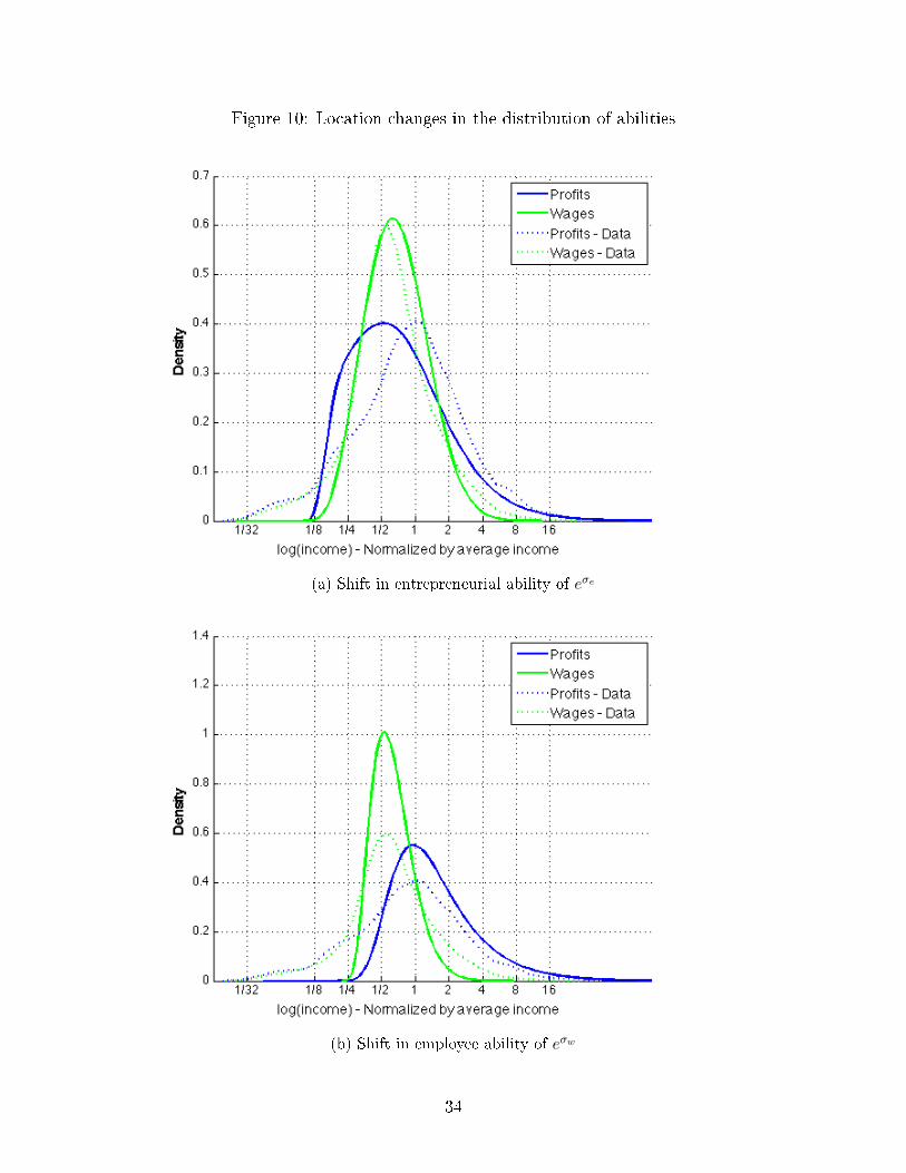
Figure 10: Location changes in the distribution of abilities

(a) Shift in entrepreneurial ability of eσe

(b) Shift in employee ability of eσw

34

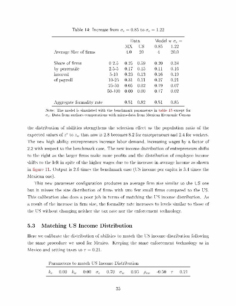
Table 14: Increase from σe = 0.85 to σe = 1.22

Data Model w σe =MX US 0.85 1.22

Average Size of �rms 4.0 20 4 20.0

Share of �rms 0-2.5 0.25 0.59 0.20 0.34by percentile 2.5-5 0.17 0.15 0.11 0.16interval 5-10 0.23 0.13 0.16 0.19of payroll 10-25 0.31 0.11 0.27 0.21

25-50 0.05 0.02 0.19 0.0750-100 0.00 0.00 0.17 0.02

Aggregate formality rate 0.51 0.82 0.51 0.85

Note: The model is simulated with the benchmark parameters in table 15 except forσe. Data from authors computations with micro-data from Mexican Economic Census

the distribution of abilities strengthens the selection e�ect as the population ratio of the

expected values of ze to zw that now is 2.8 becomes 8.2 for entrepreneurs and 2.4 for workers.

The new high ability entrepreneurs increase labor demand, increasing wages by a factor of

2.2 with respect to the benchmark case. The new income distribution of entrepreneurs shifts

to the right as the larger �rms make more pro�ts and the distribution of employee income

shifts to the left in spite of the higher wages due to the increase in average income as shown

in �gure 11. Output is 2.6 times the benchmark case (US income per capita is 3.4 times the

Mexican one).

This new parameter con�guration produces an average �rm size similar to the US one

but it misses the size distribution of �rms with two few small �rms compared to the US.

This calibration also does a poor job in terms of matching the US income distribution. As

a result of the increase in �rm size, the formality rate increases to levels similar to those of

the US without changing neither the tax rate nor the enforcement technology.

5.3 Matching US Income Distribution

Here we calibrate the distribution of abilities to match the US income distribution following

the same procedure we used for Mexico. Keeping the same enforcement technology as in

Mexico and setting taxes to τ = 0.21.

Parameters to match US Income Distribution

ke = 0.00 kw = 0.00 σe = 0.70 σw = 0.95 ρew = -0.50 τ = 0.21

35

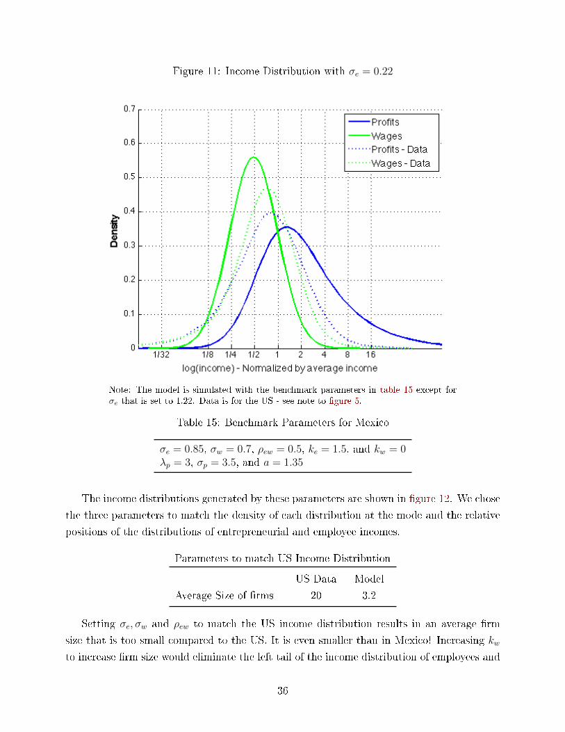
Figure 11: Income Distribution with σe = 0.22

Note: The model is simulated with the benchmark parameters in table 15 except forσe that is set to 1.22. Data is for the US - see note to �gure 5.

Table 15: Benchmark Parameters for Mexico

σe = 0.85, σw = 0.7, ρew = 0.5, ke = 1.5, and kw = 0λp = 3, σp = 3.5, and a = 1.35

The income distributions generated by these parameters are shown in �gure 12. We chose

the three parameters to match the density of each distribution at the mode and the relative

positions of the distributions of entrepreneurial and employee incomes.

Parameters to match US Income Distribution

US Data Model

Average Size of �rms 20 3.2

Setting σe, σw and ρew to match the US income distribution results in an average �rm

size that is too small compared to the US. It is even smaller than in Mexico! Increasing kwto increase �rm size would eliminate the left tail of the income distribution of employees and

36

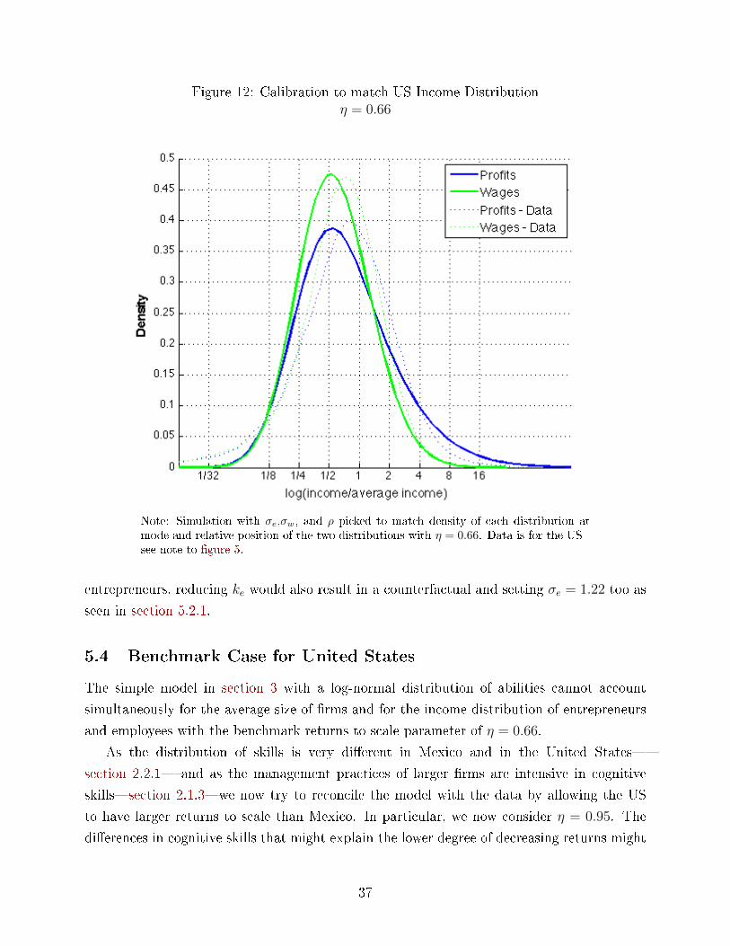
Figure 12: Calibration to match US Income Distributionη = 0.66

Note: Simulation with σe,σw, and ρ picked to match density of each distribution atmode and relative position of the two distributions with η = 0.66. Data is for the US -see note to �gure 5.

entrepreneurs, reducing ke would also result in a counterfactual and setting σe = 1.22 too as

seen in section 5.2.1.

5.4 Benchmark Case for United States

The simple model in section 3 with a log-normal distribution of abilities cannot account

simultaneously for the average size of �rms and for the income distribution of entrepreneurs

and employees with the benchmark returns to scale parameter of η = 0.66.

As the distribution of skills is very di�erent in Mexico and in the United States�

section 2.2.1� and as the management practices of larger �rms are intensive in cognitive

skills�section 2.1.3�we now try to reconcile the model with the data by allowing the US

to have larger returns to scale than Mexico. In particular, we now consider η = 0.95. The

di�erences in cognitive skills that might explain the lower degree of decreasing returns might

37

be explained in terms of a higher value of the parameters λ�expected value el the log

ability�consistent with the data en section 2.2.1.

Table 16: Benchmark Parameters for United States

η = 0.95σe = 0.075, σw = 0.85, ρew = 0.7, ke = 0, and kw = 0.03τ = 0.208, λp = 3, σp = 3.5, and a = 1.35

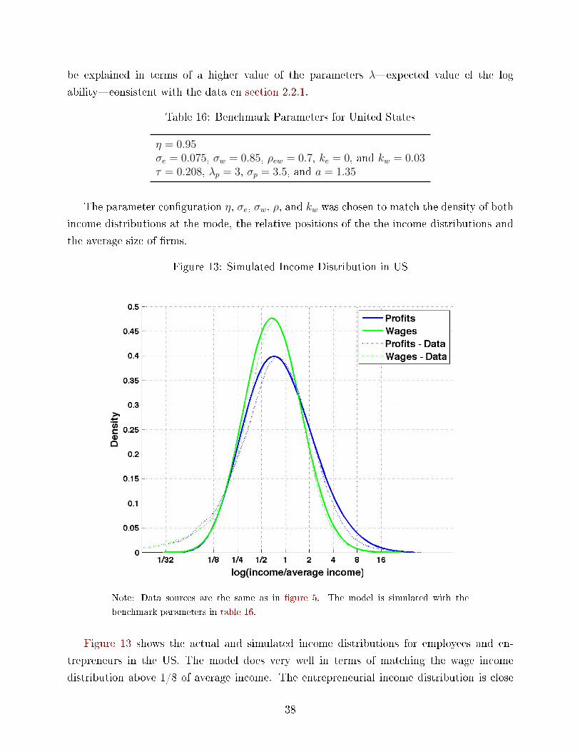
The parameter con�guration η, σe, σw, ρ, and kw was chosen to match the density of both

income distributions at the mode, the relative positions of the the income distributions and

the average size of �rms.

Figure 13: Simulated Income Distribution in US

Note: Data sources are the same as in �gure 5. The model is simulated with the

benchmark parameters in table 16.

Figure 13 shows the actual and simulated income distributions for employees and en-

trepreneurs in the US. The model does very well in terms of matching the wage income

distribution above 1/8 of average income. The entrepreneurial income distribution is close

38

to the data in the range [1/8, 4] and produces a fatter tail for upper incomes and a thinner

tail than the data for lower incomes. The di�erence between the median (log) income of

entrepreneurs and employees is 13% in the data and 3% in the model.

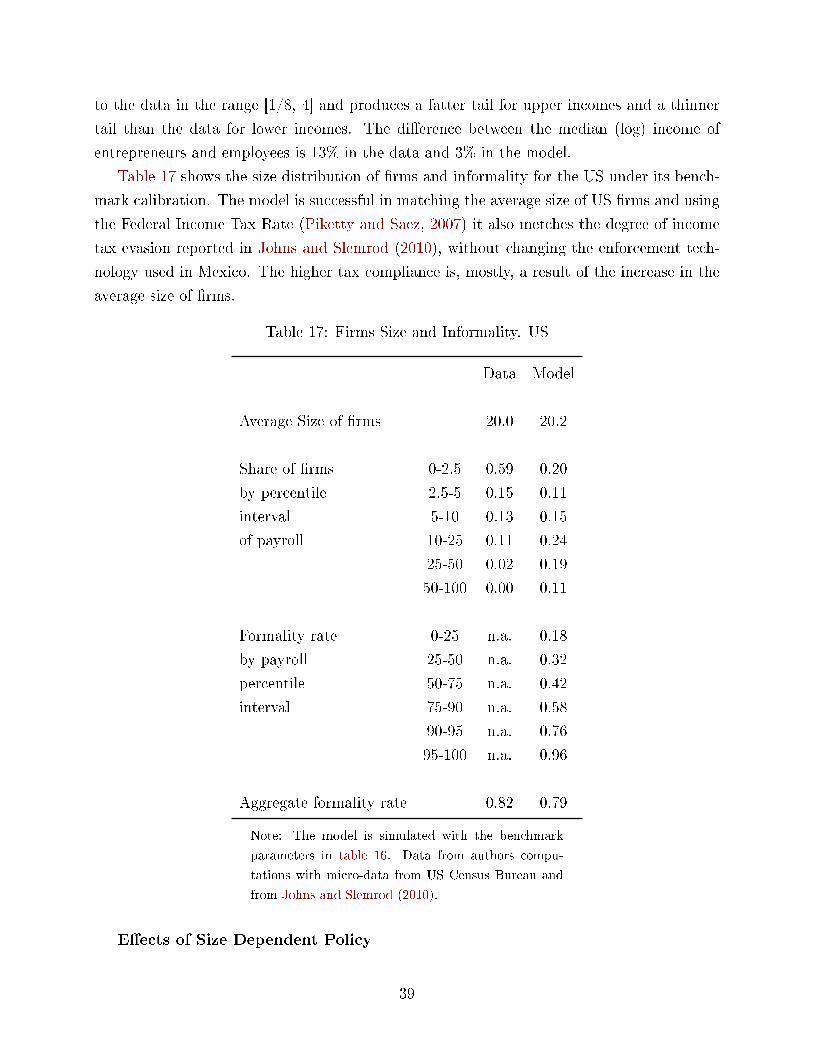
Table 17 shows the size distribution of �rms and informality for the US under its bench-

mark calibration. The model is successful in matching the average size of US �rms and using

the Federal Income Tax Rate (Piketty and Saez, 2007) it also metches the degree of income

tax evasion reported in Johns and Slemrod (2010), without changing the enforcement tech-

nology used in Mexico. The higher tax compliance is, mostly, a result of the increase in the

average size of �rms.

Table 17: Firms Size and Informality. US

Data Model

Average Size of �rms 20.0 20.2

Share of �rms 0-2.5 0.59 0.20

by percentile 2.5-5 0.15 0.11

interval 5-10 0.13 0.15

of payroll 10-25 0.11 0.24

25-50 0.02 0.19

50-100 0.00 0.11

Formality rate 0-25 n.a. 0.18

by payroll 25-50 n.a. 0.32

percentile 50-75 n.a. 0.42

interval 75-90 n.a. 0.58

90-95 n.a. 0.76

95-100 n.a. 0.96

Aggregate formality rate 0.82 0.79

Note: The model is simulated with the benchmark

parameters in table 16. Data from authors compu-

tations with micro-data from US Census Bureau and

from Johns and Slemrod (2010).

E�ects of Size Dependent Policy

39

Removing taxes while keeping the other parameters at the benchmark case the average

�rm size climbs to 46 and the e�ciency from the benchmark case with a 21% tax is 0.3% of

output.

6 Concluding Remarks

We have used a new data set from the OECDs Programme for the International Assessment

of Adult Competencies and data for Latin America to document how occupational choices

and the size distribution of �rms are related to cognitive abilities, education and income.

Then we have built a simple model of occupational choice and the size distribution of

�rms embedding a Roy Model (Roy, 1951) with two dimensional heterogeneity in a Lucas

Model (Lucas, 1978) of �rms size. We used the model to simultaneously explain the size

distribution of �rms, the income distribution of entrepreneurs and employees, and the degree

of tax compliance.

The model successfully �ts the Mexican data using a decreasing returns parameter of

2/3, which is consistent with the development literature (Hsieh and Klenow, 2009). With the

returns to scale parameter that �ts the Mexican data our simple model with a log-normal

joint distribution of abilities cannot simultaneously �t the US average �rm size and the

main patterns of the income distribution of US employees and entrepreneurs. Increasing the

returns to scale parameter to 0.95 the model �ts well the US data.

Using the same enforcement technology and tax rates derived from the data the model

�ts well the observed degree of payroll tax compliance in Mexico and in the US.

We interpret the need to increase the returns to scale parameter in the US relative to

Mexico in order to �t the data on income distribution, occupational choice and the size of

�rms as a re�ection of better management practices that permit a larger scale of operation as

documented by (Bloom and Reenen, 2007). It remains for future research to develop a model

of skills and the size distribution of skills in which the returns to scale of a �rm endogenously

depend on the skills of its workers and leaders.

References

Bigio, Saki and Eduardo Zilberman. 2011. �Optimal self-employment income tax enforce-

ment.� Journal of Public Economics 95 (9-10):1021�1035.

Bloom, Nicholas, Christos Genakos, Ra�aella Sadun, and John Van Reenen. 2012. �Man-

40

agement Practices Across Firms and Countries.� Academy of Management Perspectives

0 (0):12�33.

Bloom, Nicholas and John Van Reenen. 2007. �Measuring and Explaining Management

Practices Across Firms and Countries.� The Quarterly Journal of Economics 122 (4):1351�

1408.

Busso, Matias, Maria Victoria Fazio, and Santiago Levy. 2012. �(In)Formal and

(Un)Productive: The Productivity Costs of Excessive Informality in Mexico.� Research

Department Publications 4789, Inter-American Development Bank, Research Department.

Fiori, Anna Maria and Davide Beltrami. 2014. �Right and left kurtosis measures: large

sample estimation and an application to �nancial returns.� Stat 3 (1):95�108.

Guner, Nezih, Gustavo Ventura, and Xu Yi. 2008. �Macroeconomic Implications of Size-

Dependent Policies.� Review of Economic Dynamics 11 (4):721�744.

Hanushek, Eric A. and Ludger Woessmann. 2009a. �Do Better Schools Lead to More Growth?

Cognitive Skills, Economic Outcomes, and Causation.� NBER Working Papers 14633,

National Bureau of Economic Research, Inc.

���. 2009b. �Schooling, Cognitive Skills, and the Latin American Growth Puzzle.� NBER

Working Papers 15066, National Bureau of Economic Research, Inc.

Hsieh, Chang-Tai and Peter J. Klenow. 2009. �Misallocation and Manufacturing TFP in

China and India.� The Quarterly Journal of Economics 124 (4):1403�1448.

Johns, Andrew and Joel Slemrod. 2010. �The Distribution of Income Tax Noncompliance.�

National Tax Journal 63 (3):397�418.

Jovanovic, Boyan. 1994. �Firm formation with heterogeneous management and labor skills.�

Small Business Economics V6 (3):185�191.

Lucas, Robert E. 1978. �On the Size Distribution of Business Firms.� Bell Journal of

Economics 9 (2):508�523.

Oi, Walter Y. and Todd L. Idson. 1999. �Firm size and wages.� In Handbook of Labor

Economics, Handbook of Labor Economics, vol. 3, edited by O. Ashenfelter and D. Card,

chap. 33. Elsevier, 2165�2214.

Piketty, Thomas and Emmanuel Saez. 2007. �How Progressive is the U.S. Federal Tax

System? A Historical and International Perspective.� Journal of Economic Perspectives

21 (1):3�24.

41

Roy, A. D. 1951. �Some Thoughts on the Distribution of Earnings.� Oxford Economic Papers

3 (2):pp. 135�146.

Áureo De Paula and José A. Scheinkman. 2011. �The Informal Sector: An Equilibrium Model

And Some Empirical Evidence From Brazil.� Review of Income and Wealth 57:S8�S26.

42