D O C U M E N T O D E T R A B A J O

Instituto de EconomíaTESIS d

e MA

GÍSTER

I N S T I T U T O D E E C O N O M Í A

w w w . e c o n o m i a . p u c . c l

Global Games and Finitely Repeated Networks:The Theory and Experimental Evidence

Álvaro Parra.

2007

TESIS DE GRADO MAGISTER EN ECONOMIA

Diciembre 2007

PONTIFICIA UNIVERSIDAD CATOLICA DE CHILE I N S T I T U T O D E E C O N O M I A MAGISTER EN ECONOMIA

Global Games and Finitely Repeated Networks: The Theory and Experimental Evidence

Álvaro Parra

Comisión Augusto Castillo Rodrigo Harrison

Diciembre 2007

Global Games and Finitely Repeated Networks: TheTheory and Experimental Evidence

Álvaro G. Parra�Ponti�cia Universidad Católica de Chile

December 2007

Abstract

A �nitely repeated two-side link network is analyzed. In order to select one of multipleequilibria that arise in this kind of setting, the global game approach is used as a notion ofequilibrium. In the �rst stage of the game I restrict my analysis to particular kinds of strategies,called switching strategies. Under some restrictions on the payoff noise structure, players beliefs(and strategies) converge in the second stage of the game. This allows the game to be collapsedwith a unique equilibrium which has several nice properties. For instance, it converges to theHarrison and Elbittar (2006) global game solution when the game is played once and it con-verges to the cooperative/ef�cient solution when the game converges to an in�nitely repeatedgame. Experimental sessions testing the predictive power of the equilibrium are reported. Thepredictions of the model and comparative statics are consistent with the data. In the worst case,75% of the strategies played by individuals in the experiment can be explained by the model.

1 Introduction

The increasing interest of economists in understanding social networks stems from the recognitionthat the economic context is an important determinant of many social phenomena. The study ofnetworks have opened a door to understanding situations where the market is not the principalmechanism for the distribution of goods. Labour networks, collaboration among �rms in R &D, political agreements in the congress and, the �ow of private information are examples wherenetworks rather than markets may better explain behavior.

The main concern of networks analysis is the multiple equilibria problem. The introduction ofgraph structures and the so-called �Myerson value� by Myerson (1977) led to the study of networks

�I would like thank to Rodrigo Harrison, Roberto Muñoz and Augusto Castillo for their useful comments andencouraging and to Daniel Garret for his grammatical suggestions. Financial Support from CIDE and Ponti�cia Uni-versidad Católica de Chile is acknowledged. All mistakes are those of the author. Send comments or corrections to:agparra@northwestern.edu

1

in a cooperative context. Later, the work of Aumann and Myerson (1988) recognized that differentgraph structures led to different retributions of the agents involved in the network. Nowadays, twobranches of the study of networks can be identi�ed. One is the cooperative branch which emphasizesthe stability of the graph structure; and the noncooperative one, which emphasizes the incentives forindividuals to be part of a network (see Jackson (2003, 2007)) for a good discussion of this issueand the role of networks in economics).

Cooperative networks concepts are based on the idea that individuals can coordinate group devia-tions from their initial situations. Underpinning this behavior is some sort of communication amongindividuals (in Myerson's technical words, �individuals are path connected�.) Criticisms of thisapproach come from the argument that communication may only arise when the network is alreadyformed. So, cooperative re�nements may not be enough to explain how networks structures emerge.On the other hand, the noncooperative approach looks like a good alternative to explaining how net-works are formed, but is unlikely to explain stability of the network in the long term. Part of thiswork shows that these two approaches are not necessarily in con�ict.

Among the noncooperative concepts, the Global Game approach, introduced by Calrsson and vanDamme (1993), has shown it self to be potentially very useful in settings where multiple equilibriaarise. In few words, global games consist of turning some parameters of the game from commonknowledge to private information and using the iterative elimination of interim dominated strategiesto re�ne the set of Nash equilibria. Harrison andMuñoz (2006) show that this concept can be appliedto the network framework and, moreover, in a general setting the set of equilibria is a singleton.

The focus of this paper is to try to use the global game approach in a context where networks interacta �nite number of times and to test the model predictions under experimental sessions. My workcould be framed in an incipient literature of dynamic global games where some authors have putemphasis on learning processes as new information becomes available (see Angeletos, Hellwig andPavan (2007) for a good example) and some others concentrate their efforts on �nding conditionsof equilibrium uniqueness (see, for instance, Heidhues and Melissas (2006)), In my setting, despiteof the fact that the networks interact repeatedly, the equilibrium is similar to the static one, thoughit depends on the number of periods that the networks interact.

The experimental evidence with respect Global Games is inconclusive. On the one hand Heinemann,Nagel and Ockenfels (2004) test the Global Games predictions in a coordination game of speculativeattack and �nd that predictions are only correct under an incomplete information scheme. On theother hand Elbittar, Harrison and Muñoz (2007) test this approach in a network scheme and �ndpredictions extremely consistent with the evidence in both complete and incomplete informationcontexts. Also, noncooperative equilibria have been tested in networks by Falk and Kosfeld (2003).They found that in games where the link could be established unilaterally the strict Nash equilibriumworks very well but in games with bilateral links it doesn't.

In this paper I analyze a �nitely repeated version of the Aumann-Myerson Consent Game whichis a bilateral link network, i.e. both players must agree to be connected, however the link may besevered unilaterally. If players play essentially unique strategies in the �rst stage game and if thenoise structure has bounded support, I �nd that beliefs over other player observations (and hencestrategies) converge in the second stage of the game. This allows us to collapse all the game structureinto the �rst stage and use an approach similar to a static global game. However, individuals areforward looking, in the sense that they consider future payoffs to choose strategies that lead to a

2

unique equilibrium. Also, I test the model under experimental conditions where I �nd that, in theworst case, 75% percent of the individuals that participate in the experiment are well explained bythe model.

Section 2 describes the static consent game and its Nash equilibria. Section 3 introduces two coop-erative re�nements and the global game re�nement in order to provide background. The repeatedgame and the theoretical developments are in section 4. Section 5 presents the experimental evi-dence and section 6 concludes.

2 The Static Model

2.1 The Basic Benchmark: The Three Players Case1

Consider a static version of the Consent Game with three agents and complete information. LetI =f1;2;3g be the set of players and Ai the set of actions for player i2I where Ai=

�(ai j) j2fI nig

��ai j 2f1;0gg, for instance the action a2 = (a21 = 1;a23 = 0) 2 A2 is two's action if he attempts to estab-lish a connection with player number one and not with player three2. Since this is a two side linkformation model, a link will be formed if and only if both players try to form the link. Formally, alink between i j is formed if and only if ai j = a ji = 1.

Let x 2 R++ be a variable that scale the level of pro�ts of individuals, then the payoff function isde�ned as follows

π i(ai;a�i;x) = ai ja ji(x+a jkak jβx)+ai j(αx� c)++aikaki(x+ak ja jkβx)+aik(αx� c)

where α and β are positive �xed parameters that determine the possible revenue that a player can getgiven x; and c represents the connection attempt cost, which is also �xed and positive. Note that nomatter whether there is a link between two players, if one individual tries to establish a connectionhe will get (αx� c). Also, note that the formation of a link can only increase the total revenue ofan individual and this payoff function is symmetric in the sense that player i gets the same expectedreward if he offers a link to player j or if he offers it to player k.

Given this, the game is de�ned as the triple G(x) =I ;(Ai)i2I ;(Π)i2I

�.

2.2 The Set of Nash Equilibria

In order to obtain the best response function, lets analyze each element of the payoff function. Theterm ai j(αx� c) represents player i's cost or bene�t from attempting a link with player j. It is easy

1Taken from Harrison and Muñoz (2006)2I use notation that is standard in the literature. a�i to name the action vector of all players but i. In the same logic,

A�i = � j2fI nigA j is the action space for every individual except i. In the particular case of three players we haveA�i = A j�Ak: Lastly, I abuse notation and denote ai = 1 in order to express (ai j = 1;aik = 1) and ai = 0 to express(ai j = 0;aik = 0) :

3

to see that if x> cαthis will always be positive and it will be a dominant strategy to try a connection.

On the other side, the term ai ja ji(x) arises only when a link between players i and j is formed. Sincex > 0, this component is strictly positive. Lastly, the element ai ja ji(a jkak jβx) occurs when, givena link between i and k, there is also a link between k and j; intuitively, this component representsan indirect bene�t for the �relationship� among other players. If we understand this network asa friendship relation (as Jackson and Wolinsky (1996) does) people not only get bene�ts of theirrelations, they also get bene�ts from the friends of their friends.

In the three players case, if every link is formed, the total revenue for each individual is 2((1+α+β )x� c); thus if x < c

1+α+βis a dominant strategy to never offer a link. Is important, to determine

the set of Nash Equilibria, to know when two individuals can support a link. This occurs when(1+α)x� c � 0, that is, when x � c

1+α. Given all these elements, it is easy to show that the best

response function is:

� If x 2�

∞; c1+α+β

�, then

BRi (a�i) =�ai = 0 8a� j 2 A� j

� If x 2

hc

1+α+β; c1+α

i, then

BRi(a�i) =

8>><>>:ai = 1 if a�i = 1ai j = 1;aik = 0 if a ji = a jk = ak j = 1; aki = 0ai j = 0;aik = 1 if a ji = 0; aki = a jk = ak j = 1ai = 0 otherwise

� If x 2� c1+α

; cα

�, then

BRi(a�i) =

8>><>>:ai j = 1;aik = 1 if a ji = aki = 1ai j = 1;aik = 0 if a ji = 1; aki = 0ai j = 0;aik = 1 if a ji = 0; aki = 1ai j = 0;aik = 0 if a ji = 0; aki = 0

� If x 2� c

α;∞�, then

BRi (a�i) =�ai = 1 8a� j 2 A� j

The best response function allows us to �nd the sets of NE, which is represented in Figure 1.

r rr JJr rr

r rrr rr

r rrJJr rr

JJr rr

JJr rr

-� xc

1+α+β

c1+α

cα

Figure 1 Networks structures supported by a Nash Equilibrium. Each agent isrepresented by a node and a link is represented by a line between nodes.

4

In Figure 1 each node represents an agent (any of them) and lines between nodes represent connec-tions. The multiplicity of Nash Equilibria is evident. This leads us to think about how to establish aunique prediction. Next section introduces some re�nements concepts.

3 Proposed Re�nements

3.1 Cooperative Re�nements

Cooperative re�nements in networks are important when the focus of the analysis is propertiesof a network rather than individuals incentives. More precisely, these re�nements say somethingabout the stability of a network; Namely wether exist incentives for a network to change its form.Among the most in�uential cooperative concepts is �Pairwise Stability�, introduced by Jackson andWolinsky (1996). They say that if no pair of individuals has incentives to do a join deviation, thatis to sever or create a link, then the network is stable. Speci�cally, a Nash equilibrium is PairwiseStable if the following two conditions hold:

i) If a link between two individuals is absent from the network then it cannot be that both indi-viduals would bene�t from adding the link (with at least one bene�ting strictly.)

ii) If a link between two individual is present in a network the it cannot be that either individualwould strictly bene�t from deleting that link.

To have a better understanding of this concept let's apply it to the set of Nash equilibria for theconsent game. As Figure 2 shows, this set is re�ned; however is not strong enough to �nd a uniqueequilibrium.

r rr JJr rrr rr

JJr rr

JJr rr

-� xc

1+α+β

c1+α

cα

Figure 2 Network structures supported by a equilibrium Nash Pairwaise Stable.

The �weakness� of the previous concept comes from only allowing pairs of players to do a jointdeviation. Other re�nements with higher requirements have been developed in order to avoid themultiplicity. The Strong Stable Network introduced by Jackson and van den Nouweland (2005)permit coordinated deviations of groups of individuals and moreover, allows deviations such thatindividuals that are not part of it could be strictly worse off than the initial situation.

If we apply this stability notion to the Consent Game, the set of Nash equilibria turns to a singletonan the strategy played is a switching strategy with threshold at x= c

1+α+β. That is, for all x< c

1+α+β

nobody in the network tries to establish a connection with anybody; for all x > c1+α+β

everybodytries to connect with everyone and the complete network is formed. If x= c

1+α+β, its not clear what

5

will happen. For the last situation this strategy is called an essentially unique strategy. Figure 3shows the networks structures supported by the Strong Stable Network notion.

Criticisms of this kind of approach come from the fact that to produce coordinated joint deviationsof groups of individuals requires communication. This requirement is not too strong for individualsthat are part of an existing network but if the network does not exist or individuals are outside thenetwork, its very unlikely that this coordination can emerge. The next section analyzes this gameunder a non-cooperative scheme which is the basis of my work.

r rr JJr rr

JJr rr

JJr rr

-� xc

1+α+β

c1+α

cα

Figure 3 Network structures supported by a Strong Stable Network equilibrium.

3.2 The Global Game Re�nement

The Global Game approach uses a Bayesian version of the previous model, hence it is a BayesianNash Equilibrium concept. In order to �nd it, we need to rede�ne some concepts and developnew ones. The next example is taken from Harrison and Muñoz (2006). Assume that there is acommon value θ , which is draw uniformly from its support

�θ ;θ

�.3 However, for each individual

the level of possible revenues is scaled by xi = θ +σε i, where σ is a weight factor and ε i is therealization of a random variable with density φ and support in

��12 ;

12�. I assume that ε i is i.i.d.

across individuals.4 This produces two categories of beliefs: player i's beliefs over θ , which areθ jxi �U

�xi� σ

2 ;xi+σ

2�, and player i's beliefs over x j (given its observation,) which are x j jxi �

U [xi�σ ;xi+σ ]. A pure strategy for player i is a function from its private observation to its actionspace si :

�x� σ

2 ; x̄+σ

2�! Ai, the set of all such functions is denoted Si. The pay off function is

now

π i (si;s�i;xi) = ai ja ji(xi+a jkak jβxi)+ai j(αxi� c)++aikaki(xi+ak ja jkβxi)+aik(αxi� c)

Call this game of incomplete information G(σ).5

Let us de�ne an essentially unique switching strategy between 0 and 1 with threshold ki as a purestrategy si(�;ki) satisfying:

si(xi;ki) =�1 i f xi > ki0 i f xi < ki

Harrison and Muñoz (2006) prove the following proposition:3I use the uniform distribution only for simplicity, the authors shown that the next analysis hold with any distribution4Harrison and Muñoz develop their model in a more general payoff function context and their proofs also works if

ε i come from an i:i:d: process and it has a continuous distribution over R5This game corresponds to a private value de�nition. There is a common value de�nition where each player's pay-off

function depends of θ instead of xi

6

Proposition 1 For any σ > 0, the essentially unique switching strategy pro�le s� = (si(�;k�))i2I isthe only strategy pro�le that survives iterated elimination of strictly dominated strategies in G(σ),where k� = 4c

2+4α+ 43β.

Figure 4 shows the set of Network structures supported by BNE for the consent Game. As can beseen, there is also a switching point but it is totally different to the ones predicted by cooperativeequilibria.

r rr r rr r rr JJr rr

JJr rr

-� xc

1+α+β

c1+α

4c2+4α+ 43β

cα

Figure 4 Networks structures supported by BNE.

Harrison and Muñoz (2006) extend these results in settings with �nite numbers of players and moregeneral payoff functions. Elbittar et al. (2007) develops experimental sessions testing this gameand �nd that global game predictions are extremely consistent with the data.

4 The Repeated Game

4.1 The Model

I now introduce a repeated version of the Consent Game and incomplete information. Consider aset I = f1;2; : : : ; Ig of players and let T = f1;2; :::;Tg be the number of periods that the game

is repeated where T is �nite. De�ne Ati =��ati j�j2fI =ig

���ati j 2 f0;1g� as the action space ofindividual i in period t. Assume that there is a common value θ , which is drawn uniformly6 from itssupport

�θ ;θ

�. However, for each individual the level of possible revenues is scaled by xi= θ+σε i,

where σ is a weigh factor and ε i is the realization of a random variable with continuous density f (�)and support in a bounded interval of R. I assume that ε i is i.i.d. across individuals.

Let ati =�ati�i�be the vector of actions of player i at period t and at the vector of actions of all

players at period t. We can de�ne the observed history of the game as follow:

hti j =�atj i f ati j = 1/0 i f ati j = 0

�[ht�1i j ; with h

1i j = /0

that is, player i can observe player j's action if and only if player i tries to establish a connectionwith player j. Note that this object is de�ned recursively.

6As the previus section, I use the uniform distribution only for simplicity, it can be shown that the next analysis holdwith any distribution

7

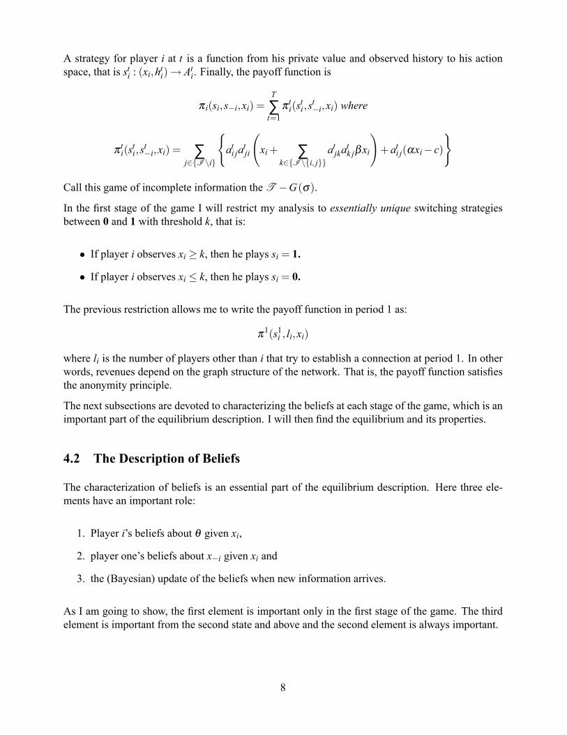
A strategy for player i at t is a function from his private value and observed history to his actionspace, that is sti : (xi;hti)! Ati. Finally, the payoff function is

π i(si;s�i;xi) =T

∑t=1

πti(sti;st�i;xi) where

πti(sti;st�i;xi) = ∑

j2fI nig

(ati jatji

xi+ ∑

k2fI nfi; jggatjka

tk jβxi

!+ati j(αxi� c)

)

Call this game of incomplete information the T �G(σ).

In the �rst stage of the game I will restrict my analysis to essentially unique switching strategiesbetween 0 and 1 with threshold k, that is:

� If player i observes xi � k, then he plays si = 1.

� If player i observes xi � k, then he plays si = 0.

The previous restriction allows me to write the payoff function in period 1 as:

π1(s1i ; li;xi)

where li is the number of players other than i that try to establish a connection at period 1. In otherwords, revenues depend on the graph structure of the network. That is, the payoff function satis�esthe anonymity principle.

The next subsections are devoted to characterizing the beliefs at each stage of the game, which is animportant part of the equilibrium description. I will then �nd the equilibrium and its properties.

4.2 The Description of Beliefs

The characterization of beliefs is an essential part of the equilibrium description. Here three ele-ments have an important role:

1. Player i's beliefs about θ given xi,

2. player one's beliefs about x�i given xi and

3. the (Bayesian) update of the beliefs when new information arrives.

As I am going to show, the �rst element is important only in the �rst stage of the game. The thirdelement is important from the second state and above and the second element is always important.

8

4.2.1 The First Stage Beliefs

Beliefs over θ From the model description we know that each player observes the signal xi =θ+σε i, where σ is a scale factor and ε i is the realization of an i.i.d random variable with continuousdensity f (�) and support in a bounded interval of R. Then, given that player i has the signal xi, heassign the probability f

�xi�θ

σ

�to the state of nature θ .

Beliefs over l1i In the context of switching strategies, the previous distribution allows me to de-scribe the probability that player i assign to l players observing a private signal x j above thresholdk and, therefore, trying to establish a connection. This probability is:Z

f�x�θ

σ

��II� l

��F�k�θ

σ

��I�l �1�F

�k�θ

σ

��ldθ

where�F� k�θ

σ

��I�l is the probability that I� l players observe a signal below k and �1�F � k�θ

σ

��lis the probability that l players observe a signal above k. Finally

� II�l�is the combinatorial of players

that can satisfy the previous requirement. Given this, the expected payoff for the �rst stage of thegame is:

I�1∑l=0

π�s1i ; l;xi

�Zf�x�θ

σ

��II� l

��F�k�θ

σ

��I�l �1�F

�k�θ

σ

��ldθ

4.2.2 Beliefs for t � 2

Since in the �rst period of the game we use the distribution of θ to get the beliefs of how manyplayers observe its private observation above the threshold point, in the second period of the gamethe distribution of θ lost its importance in the analysis. This is because the main concern of playeri is to know if player j will offer connection in the second stage but, from player j actions in periodone, player i will know if xi is above or below ki. More precisely, recall that player i observesplayer j actions if and only if ai j = 1, recall also that, in t = 1, individuals play only essentiallyunique switching strategies. Therefore, there only exist two possibilities: player one plays a1i = 1and observes a1; or player i plays a1i = 0 and does not observe anything. In the case that player iobserve a1 he will know exactly which players have an xi � ki. Also, is important to note that everyplayer who has an xi � ki discovers in t = 2 all other players with observation above the thresholdspoint and this is common knowledge among players. Using all these elements I am going to provethe following proposition.

Proposition 2 Let T �G(σ) be de�ned as above. Then for suf�ciently small σ beliefs over otherplayer actions converge in the second stage of the game.

Proof. In order to prove this proposition we have to analyze three cases. First, note that if a playergets an xi � ki he offers no links and he gets no new information about other player actions, so hehas no beliefs update either. Then, if in period one his observation does not survive to the iterative

9

elimination of interim dominated strategies, his observation will not survive in the second stageeither and he will offer no connections (also note that the argument holds for later periods too). The�rst case is when player i plays a1i = 1 and all other players do not try to connect, that is a1�i = 0.If this is the case, player i beliefs about other players actions are Prt�2i

�at�i = 0 jhti;xi

�= 1. The

second case is when player i plays a1i = 1 and all other players do connect, that is a1�i = 1. If thisis the case, player i beliefs of other players actions are Prt�2i

�at�i = 1 jhti;xi

�= 1. The last and

more complex case is when some players other than i offer connections but not all of them. Recallfrom the description of Nash equilibrium that a player does not want to serve a connection in anscenario where the complete network is not formed if and only if xi � c

1+α. The question that arises

in this contexts is, given that player i observes xi � c1+α

, what is the probability of the connectedplayers have an x j � c

1+α? For games with suf�ciently small σ and ε i with bounded support this

probability is 1. To see this look at Figure 5. The limits of the support of player i beliefs over otherplayer observations is a function of σ , it is possible to �nd σ i such that for all σ � σ i the supportof player i beliefs over other player observation is always above c

1+α. Then if we take the minimum

σ i among players the statement holds for all players and Prt�2i�atji = 1

��h1i ;xi� = 1, where j is aplayer that offered connection in the �rst period. In the case where xi < c

1+αplayer i wants so sever

the connection, and for suf�ciently small σ every player want to do the same.

- �c1+α

][

][xi

rr σ < σ i

σ > σ i

Figure 5: Support of the beliefs of other player private value for a player observing xi � c1+α

fordi¤erent σ .

The previous proposition allow us to state:

Proposition 3 Let T �G(σ) be de�ned as above. Then, for suf�ciently small σ , each pro�le S1has associated only one pro�le St for t � 2, such that it is the best response to each player beliefs.

Proof. For regions of xi where a dominant strategy exists, the result trivially holds. If player i playsa1i = 0, he has no new information and we will play ati = 0 for all t. If player i plays a1i = 1 and heobserves that a1�i = 0, then he will assign Pr

t�2i�at�i = 0

��h1i ;xi �= 1 and he will play ati = 0 for allt � 2. If player i plays a1i = 1 and he observes that a1�i= 1, then he assign Pr

t�2i�at�i = 1

��h1i ;xi �= 1and he will play ati = 1 for all t � 2. If player i plays a1i = 1, the complete network is not formedand xi � c

1+α, then for connected players he will believe that Prt�2i

�atji = 1

��h1i ;xi�= 1 and his bestresponse is to connect to those players and no to connect with players that have-not offer a link inthe previously period. If player i plays a1i = 1 and xi <

c1+α

, then his best response is not to offerany connection.

Corollary 4 Strategies in t � 2 for individuals that offered connection in t = 1, can be representedas a function from l1 and xi, that is:

sti : (l1;xi)! Ati

10

Proof. This function is

sti =

8>>>><>>>>:i f l1 = 0 then sti = 0i f l1 = I�1 then sti = 1

i f 0< l1 < I�1 and xi < c1+α

then sti = 0

i f 0< l1 < I�1 and xi � c1+α

�i f a1j = 0 ! ai j = 0i f a1j = 1 ! ai j = 1

stating the corollary.

This corollary is very useful, since allows us to describe all the strategies pro�les for t � 2 as afunction of l1. Therefore, payoffs of all periods are fully characterized by l1. I am going to use thisto �nd the equilibrium in the next section.

4.3 The Global Game Re�nement

The equilibrium notion developed in this section closely follow Global Games. The main differenceis that in this setting a repeated game is played. However, at is was shown in the last section, gamepayoffs and strategies are fully determined in the �rst period of the game. So, we can use the staticglobal game approach to �nd the equilibrium.

Let's de�ne ∆π i(l1;xi) = π i (1; l1;xi)�π i (0; l1;xi). Note that π i (0; l1;xi) = 0 for all l1 and xi, hence∆π i(l1;xi) = π i (1; l1;xi). With this we can state the next proposition.

Proposition 5 The payoff function satis�es the following properties

P5.1 Strategic Complementarities: ∆π(l1;xi) is increasing in l1.

P5.2 State Monotonicity: ∆π(l1;xi) is increasing in x.

P5.3 Single Crossing: There is a unique k� solving ∑I�1l=01I∆π (l;k) = 0.

P5.4 Limit Dominance: There exist x 2R++ and x 2R++ such that [1]∆π (l1;x)< 0 for all l1 andx� x; and [2]∆π (l1;x)> 0 for all l1 and x� x̄.

P5.5 Continuity: ∑I�1l=0 g(l)∆π (l1;x) is continuous with respect to signal x and density g.

The proof is relegated to the appendix A. These properties are very standard in the Global Gameliterature, see Morris and Shin (2002) or Frankel et al. (2003), and give us suf�cient tools to provethe next theorem, which is the main result of this work.

Theorem 6 LetT �G(σ) be de�ned as above. Then , for suf�ciently small σ , the set of essentiallyunique switching strategies with threshold at k is singleton, where k satis�es:

I�1∑l=0

1I

∆π (l;k) = 0 (1)

and is the only strategy that survives to the iterative elimination of strictly dominated strategies.

11

-�

6

?

����������

s

c1+α+β

cα

c1+α+β

cα

kk�

br (k�)

br (�)

45�)����������

Figure 6: The best response function is a continuous function from the compact set [x; x̄] to itself, then a �xed point exists which is represented by the point where the two sequences of the

proof converges.

Proof. This proof has two steps. The �rst is to prove that the set of strategies is singleton, the secondis to prove that the threshold point is de�ned by (1). Step one: By symmetry all players have thesame threshold point, i.e. ki = k. Let's de�ne π� (x;k) as the expected utility of a player that offerconnection to every one, observe x and other players plays the threshold k.

π� (x;k) =

I�1∑l=0

Zf�x�θ

σ

��II� l

��F�k�θ

σ

��I�l �1�F

�k�θ

σ

��ldθπ (1; l;x)

note that by P5.1 and P5.2 the previous de�nition is strictly increasing in x and strictly decreasingin k. With this, we can de�ne two sequences

ξ n+1 =min�x : π�

�x; ξ̄ n

�= 0and ξ 0 = x

ξ n+1 =max�x : π�

�x; ξ̄ n

�= 0and ξ 0 = x

the �rst sequence represent the iterative elimination of strictly dominated strategies starting fromthe upper dominance region and the second represent the same concept from the lower dominanceregion. Note, for the same argument exposed above, that the �rst sequence is strictly decreasing andthe second is strictly increasing. By construction, the sequences satisfy ξ n+1� ξ n+1 for all n, whichmeans that are two monotone sequences de�ned in a bounded interval, then both sequences mustconverge. Moreover, the must converge to the same point, hence the equilibrium is unique. To provethe last claim let's call limn!∞ ξ n+1 = ξ and limn!∞ ξ n+1 = ξ . Take an x 2

�ξ ;ξ

�, by continuity

(P5.5) and the de�nition of ξ and ξ implies π��x;ξ�> 0 and π�

�x;ξ�< 0, respectively, which is

an contradiction, so ξ = ξ . In other words, when x= k

π� (x;x) =

I�1∑l=0

Zf�x�θ

σ

��II� l

��F�x�θ

σ

��I�l �1�F

�x�θ

σ

��ldθ∆π (l;x) = 0

Second Step: I have to show thatZf�x�θ

σ

��22� l

��F�k�θ

σ

��2�l �1�F

�k�θ

σ

��ldθ =

1I

12

when x= k. For this just take the the integral by parts and the result holds. So, we �nally get

I�1∑l=0

1I

∆π (l;x) = 0

which exist by P5.3. Figure 6 shows a picture of the intuition of this result

4.4 Properties of the Equilibrium for three Players

This section characterizes some properties of the equilibrium for the three player case. Motivationsfor this are simplicity (our benchmark is constructed under a three player scheme,) tractability anddeveloping the theoretical �ndings that are tested in the experimental section. Appendix A showthat all this results can be extended to the I players case.

Corollary 7 The threshold point k in a game with three players and length T is:

k� (T ) =

(" 2c(2+T )(2(T )+1)+2α(2+T )+2(T )β i f 32β � T

3c(1+T )3T+3α(1+T )+2Tβ

i f 32β � T

#

Proof. From proposition 6 we know

2

∑l=0

13

∆π (l;x) = 0

Its important to note that strategies in t � 2 are conditioned to which interval is k�. If k� 2hc

1+α+β; c1+α

iequation (1) becomes:

132T [(1+α+β )x� c]+ 1

3[(1+2α)x�2c]+ 1

32 [αx� c] = 0

and implies

k (T )� =2c(2+T )

(2T +1)+2α (2+T )+2Tβ

If k� 2� c1+α

; cα

�equation (1) becomes:

132T [(1+α+β )x� c]+ 1

3[T ((1+α)x� c)+αx� c]+ 1

32 [αx� c] = 0

and implies

k (T )� =3c(1+T )

3T +3α (1+T )+2Tβ

It can be easily shown that the �nal solution is:

k� (T ) =

(" 2c(2+T )(2(T )+1)+2α(2+T )+2(T )β i f 32β � T

3c(1+T )3T+3α(1+T )+2Tβ

i f 32β � T

#

13

Since my approach is close to Global Games, it is desirable to both solutions coincide if T = 1. Thenext corollary state this result.

Corollary 8 When T �G(σ) has three players and T = 1, the solution converges to the GlobalGame solution.

Proof. Just take T = 1,

k� (T ) =

(" 4c2+4α+ 43β

si 32β � T4c

2+4α+ 43βsi 32β � T

#which is the static solution.

Harrison and Muñoz (2006) show that in a set of payoff functions satisfying a weaker version ofproposition 5 the set ef�cient solution, i.e. where the summation over all players payoff is maxi-mized, is a switching strategy at the lower dominance point, in this case x = c

1+α+β. Is interesting

to see that, in the limit, when the repeated game converges to a in�nitely repeated game, the non-cooperative switching point is the ef�cient solution.

Corollary 9 When T �G(σ) converges to an in�nitely repeated game, the optimal strategy is toplay the ef�cient/cooperative solution.

Proof. Take the limit when T ! ∞

limT!∞

k� (T ) =

(" c1+α+β

si 32β � Tc

1+α+ 23βsi 32β � T

#

However, if T ! ∞ only the case 32β � T holds, so limT!∞

k� (∞) =c

1+α+β

which is the ef�cient solution.

This result has an especial importance since, in certain way, we are �nding a noncooperative foun-dation for cooperative notions of equilibrium and, moreover, this behavior is ef�cient.7

The purpose of the next section is to explain the experimental session designed to test the pre-dictability of the previous model.

7However, its not clear for the author if this is just a feature of this setting, a coincidence or if there is a generalprinciple that can be proved

14

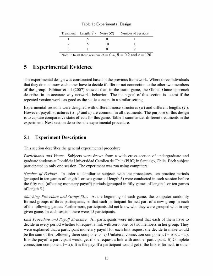
Table 1: Experimental Design

Treatment Length (T ) Noise (σ ) Number of Sessions

1 5 0 12 5 10 13 1 0 2

Note 1: In all these sessions α = 0:4; β = 0:2 and c= 120

5 Experimental Evidence

The experimental design was constructed based in the previous framework. Where three individualsthat they do not know each other have to decide if offer or not connection to the other two membersof the group. Elbittar et all (2007) showed that, in the static game, the Global Game approachdescribes in an accurate way networks behavior. The main goal of this section is to test if therepeated version works as good as the static concept in a similar setting.

Experimental sessions were designed with different noise structures (σ ) and different lengths (T ).However, payoff structures (α; β and c) are common in all treatments. The purpose of this designis to capture comparative static effects for this game. Table 1 summarizes different treatments in theexperiment. Next section describes the experimental procedure.

5.1 Experiment Description

This section describes the general experimental procedure.

Participants and Venue. Subjects were drawn from a wide cross�section of undergraduate andgraduate students at Ponti�cia Universidad Católica de Chile (PUC) in Santiago, Chile. Each subjectparticipated in only one session. The experiment was run using computers.

Number of Periods. In order to familiarize subjects with the procedures, ten practice periods(grouped in ten games of length 1 or two games of length 5) were conducted in each session beforethe �fty real (affecting monetary payoff) periods (grouped in �fty games of length 1 or ten gamesof length 5.)

Matching Procedure and Group Size. At the beginning of each game, the computer randomlyformed groups of three participants, so that each participant formed part of a new group in eachof the following games. Furthermore, participants did not know who they were grouped with in anygiven game. In each session there were 15 participants.

Link Procedure and Payoff Structure. All participants were informed that each of them have todecide in every period whether to request a link with zero, one, or two members in her group. Theywere explained that a participant monetary payoff for each link request she decide to make wouldbe the sum of the following three components: i) Unilateral connection component (= α � x� c):It is the payoff a participant would get if she request a link with another participant. ii) Completeconnection component (= x): It is the payoff a participant would get if the link is formed, in other

15

words, if both parts request the link. iii) Indirect connection component (= β �x): It is the payoff aparticipant would get if the agent she has established a link has also established a link with the thirdagent of the group. Finally, they were also informed that in case a participant has decided do notmake any link request, her monetary payoff would be zero for that period.

Valuation Distribution. For the complete information setup, all participants were informed that everymember of her group would receive in every game a connection value, x, which remain constant inevery period for game with length over than one, generated randomly by the computer from theinterval 50.00 to 310.00 and any value in this interval would have an equally likely chance of beingdraw. For the incomplete information setup, all participants were informed that every member of hergroup would privately receive in every period a connection value, xi, generated by the computer inthe following manner: i) In each period and for every group, a number, x0, would be drawn randomlyfrom the interval 50.00 to 310.00 and any value in this interval would have an equally likely chanceof being draw. ii) Once x0 was determined, each group member would receive a private connectionvalue, xi, independently selected within the interval [x0�σ ;x0+σ ], such that any value in thisinterval would have an equally likely chance of being draw. Furthermore, participants did not knowthe value of x0 nor the private value of any other participant in their group, unless the value of σ

were zero for the session.

Parameter Values.All participants were informed at the beginning of the session the values for alpha(α), beta (β ), connection cost (c), sigma (σ ) and game length (T .)

Minimum Capital and Payoff Procedure. Each participant received an initial points balance of 9,000points. Participants were paid the total points earned (or lost) from each decision period, plus theinitial point balance, multiplied by $0.33 Chilean pesos per point at the end of the experiment.The average payoff per participant for the whole session was $5,250 Chilean pesos (about 11.0 USdollars).

Information Feedback. In every period, each participant observed only her own payoff coming fromeach of the other members of her group and discriminated by each of the three payoff componentsalready mentioned. Communication among the participants was not allow throughout all sessions.They could not see each others' screens.

5.2 Experimental Results

The �rst element tested was the restriction of focusing only in essentially unique switching strategiesat period one. Using a Bernoulli distribution in order to describe each player action, the probabilityof observing a switching strategy has a binomial distribution.

Result 1 At most the probability of observing a non essentially unique strategy in the �rst stage is13%.

Table 2 shows statistics and con�dence intervals for this test in all treatments. As can be seen, we canreject the hypothesis that only essentially unique strategies where played. However, the proportionof those strategies is very high, at least around the 90% of the strategies played is essentially unique.

16

Table 2: Statistics for non-essenially unique strategies

Treatment Session Mean Variance Con�dence Interval�

T = 5;σ = 0 1 2.67% 0.0173% [0:09%;5:24%]T = 5;σ = 10 1 10.00% 0.0600% [5:20%;14:80%]T = 1;σ = 0 1 6.93% 0.0086% [5:12%;8:27%]T = 1;σ = 0 2 12.00% 0.0141% [9:67%;12:89%]�95% of con�dence

0 100 200 300 4000

0.25

0.5

0.75

1Pr(y=1|x)

x

pr

0 100 200 300 4000

0.25

0.5

0.75

1Pr(y=0|x)

x

pr

0 100 200 300 4000

0.25

0.5

0.75

1

x

pr

0 100 200 300 4000

0.25

0.5

0.75

1

x

pr

0 100 200 300 4000

0.25

0.5

0.75

1

x

pr

0 100 200 300 4000

0.25

0.5

0.75

1

x

pr

T = 5sigma = 0

T = 5sigma = 10

T = 1sigma = 0

Figure 7: Accumulative link request probability for di¤erent treatments.

The next step in the analysis is to determine which is the threshold point of the switching strate-gies. A Logit model was used with the purpose to �nd the probability of offer connection with all

17

Table 3: Logit Model Result for Individual Link Request Probability for di¤erent game lenght

Link Request ProbabilityCoef�cients T = 1;σ = 0 T = 5;σ = 0 T = 5;σ = 0Intercept -6.243� -6.185� -4.461�

(.2523) (0.965) (.6338)x .0491� .0751� .0428�

(.0019) (1.096) (.0054187)Number of Obs. 3000 300 300Number of Ind. 30 15 15Log Likelihood -729.34338 -47.7 -77.6� p< 0:001: Note: The number in parentheses below eachcoef�cient represent the coef�cient standard error.

Table 4: Statistics for Switching Thresholds

Treatment Session x k� �k Interval�

T = 5;σ = 0 1 75 90 82 [62;122]T = 5;σ = 10 1 75 90 105 [84;140]T = 1;σ = 0 1 75 124 126 [116;135]T = 1;σ = 0 2 75 124 120 [114;134]�95% of con�dence

individuals:8

Pr�s1i = 1 jxi

�= G(γ0+ γ1xi) ; where G(z) =

ez

(1+ ez)

The results of these regressions are summarized in Table 3. As it can be seen, all parameters aresigni�cant at 1%. Figure 7 shows the accumulative distribution of both strategies, s1i = 1 in the �rstcolumn and s1i = 0 in the second column.

Result 2 In all treatments the predicted switching point is in the interval of con�dence.

To �nd the switching point I look at the point where Pr�s1i = 1 jxi

�= Pr

�s1i = 0 jxi

�= 50%. Table

4 shows the starting point of the lower dominance region (x,) the predicted switching point (k�,)the estimated switching point (�k) and its con�dence interval for each treatment. As can be seen,estimated parameters change according the theory, furthermore they always are in the con�denceinterval.

The last element tested is the convergence of sti for t � 2. With this purpose two measurements werecreated. The �rst one is a binomial distribution where the random variable takes the value of y= 1if the pro�le sti changes after the second period and y = 0 if it do not change. With this measure I

8I also used a Multinomial Logit and a Ordered Logit. All methods have its advantage and problems. However,regressions were extremely robust. The three models predicts almost the same switching point in each treatments.

18

Table 5: Statistics for Switching Thresholds

Treatment Session Mean Standard Deviation Con�dence Interval�

Among Pro�lesT = 5;σ = 0 1 23.33% 1.99% [19:43%;27:24%]T = 5;σ = 10 1 27.22% 3.64% [20:20%;34:46%]

Within Pro�lesT = 5;σ = 0 1 12.22% 1.54% [9:20%;15:25%]T = 5;σ = 10 1 14.88% 1.68% [11:59%;18:17%]�95% of con�dence

capture the essence of proposition number 3. The second one is also a binomial distribution wherethe random variable takes the value of y = 1 if sti 6= st�1i for t � 3 and y = 0 if sti = st�1i for t � 3.This second measure shows the frequency of change inside a pro�le. If all strategies change in everyperiod then this measure takes the value of 1 and if it never change, takes the value of 0.

Result 3 At least the 75% of the strategies pro�les converges.

As Table 5 shows, the �rst measurement is around 25%. This implies that a fourth of the strategiesdoes not converge in the second stage. However, the variation inside strategies is low. This lead usto think that strategies converge in later stage of the game.

6 Conclusions

Despite off the fact that this game collapse in the �rst stage, it is interesting to remark that the �naloutcome depends on the game length. As greater the number of time that the stage game is repeatedthe lower will be the switching point. The relevance of this result increase when the limit whenT goes to in�nity is taken because the cooperative/ef�cient solution arises. This result could beunderstand as a bridge between the cooperative and the noncooperative literature in networks whichremained unrelated up to this point. Further efforts could be done in this area in order to determinewhich are the determinant factors of this result.

Under the experimental point of view, the fact that at least the 75% of the population that partici-pated in the experiment is explained by the theoretical framework described in this paper add moreevidence to the potential of the global game approach. However, since I have few sessions andtreatments this evidence should be taken carefully.

Further research could focus on drop main assumptions of this work like xi remains constant throwthe stage of the game or use a more general payoff function and study some applications. Undermy point of view, a productive �eld could be industrial organization where this framework can beapplied to understand market structures or asymmetries between the entrance or the exit of a �rm inmarket.

19

A Appendix: Omitted Proofs

A.1. Proof of Proposition 5

1. Strategic Complementarities: Holds since α and β are positive.

2. State Monotonicity: Just take the derivative.

3. Limit Dominance: I found it in section 2 and their are x= c1+α+β

and x̄= cα.

4. Continuity: Since f (�) is continuos, g(�) is continuous too. ∆π is continuos, since π iscontinuos. And the composition of continuos functions is continuos.

5. Single Crossing: Since ∆π(l;xi) is continuous in x and exists limit dominance. Then, forcentral theorem of calculus must exist an x such that ∑2l=0

1I∆π (l;x) = 0�

A.2. Equilibrium Properties for I Players.Analytic Solution for T Periods and I Players

The payoff of offer connection to everyone, given xi, and l players distinct that i get connected is.

π i(1; l;xi) = l (xi+(l�1)βxi)+(I�1)(αxi� c)

So, for k 2h

c1+α+β

; c1+α

i, equation (1) is:

I�2∑l=0

l (xi+(l�1)βxi)+(I�1)(αxi� c)I

+T ((I�1)(xi (1+α)� c+(I�2)βxi))

I= 0

Which implies

k (I;T ) =�

6c(I+T �1)3(2T + I�2)+6α (T + I�1)+2β (6�6T �5I+ I2+3TI)

�

For k 2� c1+α

; cα

�, equation (1) is:

I�1∑l=0

T l (xi (1+α)� c+(l�1)βxi)+(I�1� l)(αxi� c)I

= 0

which implies

k (I;T ) =�

3c(1+T )3T +3α (1+T )�2βT (2� I)

��

Convergence to the static solution (T = 1)

20

Both solutions for the static game are

k (I;1) =

8<:6c(I)

3(I)+6α(I)+2β(�2I+I2)i f k 2

hc

1+α+β; c1+α

i6c

3+6α�2β (2�I) i f k 2� c1+α

; cα

�9=;�

Convergence to the ef�cient Solution

The ef�cient solution iske f f =

�c

α+β (I�2)+1

�and the limit for the relevant interval is:

limT!∞

k (I;T ) =�

c1+α+β (I�2)

��

21

References

[1] George-Marios Angeletos, Christian Hellwig & Alessandro Pavan (2007): "Dynamic GlobalGames of Regime Change: Learning, Multiplicity and Timing of Attacks," Econometrica, vol.75(3), pages 905-22, May.

[2] Aumann, R. (1959) �Acceptable Points in General Cooperative n-Person Games,� in H. W.Kuhn and R. D. Luce, eds., Contributions to the Theory of Games IV, Princeton: PrincetonUniversity Press, 287-324.

[3] Aumann, R. and R. Myerson (1988) �Endogenous Formation of Links Between Players andCoalitions: An Application of the Shapley Value,� The Shapley Value, A. Roth, CambridgeUniversity Press, 175-191.

[4] Benoit, J.P. & Krishna, V. (1985) "Finitely Repeated Games," Econometrica, vol. 53(4), pages905-22, July.

[5] Carlsson, H. and E. van Damme (1993) �Global Games and Equilibrium Selection,� Econo-metrica, Vol. 61(5), 989-1018.

[6] Dasgupta, Amil (2006): �Coordination and Delay in Global Games� Journal of EconomicThe-ory, forthcoming.

[7] Dutta, B. and S. Mutuswami (1997) �Stable Networks,� Journal of Economic Theory, 76, 322-344.

[8] Elbitar, A., Harrison, R. and R. Muñoz (2007) �Network Structure in a Link Formation Game:An Experimental Study�, working paper.

[9] Frankel, D., S. Morris and A. Pauzner (2003) �Equilibrium Selection in Global Games withStrategic Complementarities,� Journal of Economic Theory, 108, 1-44.

[10] Fudenberg, D. & Tirole, J. 1991 "Game Theory," Cambridge, MA: MIT Press.

[11] Harrison, R. and R. Muñoz (2006) �Stability and Equilibrium Selection in Link FormationGames�, working paper Universidad Católica de Chile and Universidad Federico Santa María.

[12] Heidhues, Paul, and Nicolas Melissas (2006): �Equilibria in a Dynamic Global Game: TheRole of Cohort Effects�, Economic Theory, 28, 531-557.

[13] Heinemann. F, Nagel, R and Ockenfels, P. (2004): "The Theory of Global Games on Test:Experimental Analysis of Coordination Games with Public and Private Information. Econo-metrica, Vol. 72, No 5, 1583-1599.

[14] Jackson, M.O, (2003) �The Study of Social Networks In Economics,� forthcoming in TheMissing Links: Formation and Decay of Economic Networks, edited by Joel Podolny andJames E. Rauch.

[15] Jackson, M.O, (2005) �Network Formation,� in The New Palgrave Dictionary of Economicsand the Law, MacMillan Press, forthcoming.

22

[16] Jackson, M. and A. van den Nouweland (2005) �Strongly Stable Networks,� Games and Eco-nomic Behavior, 51(2), 420-444.

[17] Jackson, M. and A. Wolinsky (1996) �A Strategic Model of Social and Economic Networks,�Journal of Economic Theory, 71, 44-74.

[18] Morris, S. and H. Shin (2002) �Global Games: Theory and Applications,� in Advances inEconomics and Econometrics (Proceedings of the Eight World Congress of the EconometricSociety), ed. by M. Dewatripont, L. Hansen, and S. Turnosky. Cambridge, England: Cam-bridge University Press.

[19] Myerson, R. (1977) �Graphs and Cooperation in Games,�Math. Operations Research, 2, 225-229.

[20] Myerson, R. (1991) Game Theory: Analysis of Con�ict, Harvard University Press: Cam-bridge, MA.

[21] Riordan, J. (1968) Combinatorial Identities, Wiley Series in Probability and MathematicalStatistics.

23