D O C U M E N T O D E T R A B A J O

Instituto de EconomíaTESIS d

e MA

GÍSTER

I N S T I T U T O D E E C O N O M Í A

w w w . e c o n o m i a . p u c . c l

Wives’ Economic Independence and Marital Stability:Evidence from Chilean Households between 1996 and 2006

Pascale Vignau L.

2010

Pontificia Universidad Católica de Chile

Instituto de Economía

Tesis de Grado

Wives’ Economic Independence and Marital Stability:

Evidence from Chilean Households between 1996 and 2006

Agosto 2010

Nombre: Pascale Vignau L. (pvignau@gmail.com)

Programa: Magíster en Economía

Número de Alumno: 09112731

Comisión: Matías Tapia, Francisco Gallego y Klaus Schmidt-Hebbel

Abstract: This paper studies the effect of wives‟ income on the probability of divorce in

Chile through a cross section study using data from the Panel Casen between 1996 and 2006.

Becker‟s Unitary model of marriage and divorce as well as Nash Household Bargaining

models predict a positive effect of wives‟ income on the probability of divorce, a proposition

that is often called Independence Hypothesis. I estimate the probability of divorce through a

Probit model with Heckman‟s correction method for sample selection and I use instrumental

variables to solve the endogeneity of wives‟ income. The results show a positive correlation

between wives‟ income and the probability of divorce, however the effect of wives‟ income

as a percentage of total household income is inconclusive. Moreover, this investigation

studies the effect that the Chilean divorce law (2004) could have on the relationship between

wives‟ income and the odds of divorce finding that the law diminishes the effect of wives‟

income on divorce, especially in higher income families.

2

Contents

1 Introduction ..................................................................................................................... 3

2 Context ............................................................................................................................ 6

3 Literature review ............................................................................................................. 8

4 Theoretical Background ................................................................................................. 13

5 Empirical Approach ....................................................................................................... 22

5.1 Empirical Model and Method of Analysis ................................................................24 5.2 Data, Variable Description and Expected Results .....................................................27

6 Results ........................................................................................................................... 36

7 Conclusion..................................................................................................................... 48

8 References ..................................................................................................................... 50

9 Appendix ....................................................................................................................... 54

3

1 Introduction

Chilean household demography has gradually changed throughout the years. The participation

of women in the labour market is becoming more and more common while at the same time

the divorce rates have risen considerably. The last figures of the Chilean national institution

of statistics (INE) show that more than half of the marriages end up separated and that

marriage annulations have doubled in comparison to 19801. Given this evidence, a natural

question that arises is whether there is a causal relation between wives‟ economic

independence and the probability of divorce. This paper will address this question by

analysing Chilean household through data from the Panel Casen survey (1996-2006) that

covers regions III, VII, VIII and the Metropolitan region of Chile.

Figure 1 shows the trend of women‟s insertion to the labour market over the last 25 years in

Chile. The trend is positive and constant. The following investigation will concentrate on the

effect that this positive trend could have on the structure and economics of the Chilean

household.

Figure 1: Trend of Percentage of Active and Employed Women in Chile (1986-2010)

Source: INE 2010

Gary Becker has been one of the main contributors to Family Economics. This investigation

regards the decisions of marriage and divorce and Becker‟s contribution to this area of study

is vast. He states that a couple will get married if the utility of being married dominates the

utility of staying single, and the same mechanism will prevail in case of divorce (Becker,

1973). In the same paper, Becker argues that gains from marriage are derived from the

1 Marriage annulations changed from 3,6% of total marriages in 1980 to 8,5% in 1998.

4

specialization of labour within marriage, which will depend on the ratio of the spouses‟ labour

income.

Economic theories of marriage involve a strong correlation between returns to labour and

returns to marriage. It is clear that income plays an important role in the decision of getting

married and divorced but the specific causal effect is unclear. Concerning the correlation

between wives‟ income and divorce, some investigations find a positive relation (Kesselring

and Bremmer, 2006; Liu and Vikat, 2004) and others do not find any statistically significant

effect (Sayer and Bianchi, 2000; Spitze and South, 1985) so the aggregate deduction is

uncertain.

The purpose of this investigation is to study the relation between the wives‟ economic

situation and the likelihood of divorce in Chile. The idea is to analyse how the initial situation

of a couple could have an effect on their probability of getting divorced in the subsequent 5

years. Evidently the inclusion of a divorce law in Chile in 2004 implies an alteration in the

investigation so the correlation will be studied independently during a period of time before

and after the law has come into force.

Most studies in this specific area investigate the relationship between the wives‟ income or

decision to join the workforce and divorce in the US (Rogers, 2004; Booth et al., 1984) or

other developed countries (Kraft and Neimann, 2009; Liu and Vikat, 2004; Jalovaara, 2003).

Some of these studies include more explanatory variables such as “empty nest”2 (Heideman et

al., 1998) or specifically check for the effectiveness of the most commonly known barriers to

divorce (Knoester, 2000). Other investigations (e.g. Nock, 1995 and Sanhueza et al., 2007)

use cross-section data, generating a problem that could lead to loss of information. This

problem refers to effects of studying time changing variables (such as marital state) only in

one moment of time. These investigations study people‟s actual marital status without

knowing when the marriage or divorce occurred, making it difficult to state if the marital

status caused the economic situation or if the effect was the opposite. The paper at hand will

use panel data to construct the variable “divorce” to prevent this loss of information and

produce more precise estimations. Moreover, it will use data from the Chilean household

survey, which makes it pioneer in the literature. There is only one similar study done with

Chilean data (Sanhueza et al, 2007) but it studies the determinants of divorce in general, and it

does not include the effect of wives‟ income. Besides, it has some drawbacks provoked by

2 Empty-nest syndrome is the name given to a psychological condition that can affect a woman around the time

that one or more of her children leave home.

5

using cross-section data because, as explained above, then it is difficult to infer if income

caused divorce or vice versa.

The paper at hand augments the literature in several other methodological aspects. This

investigation deals with the potential selection bias that “being married” means for the study

of divorce. The variables that determine marriage will indeed determine divorce also so the

selection bias will be corrected by using an adaptation of Heckman‟s correction method for

binary response models. This study also corrects the potential endogeneity of wives‟ income

on the probability of divorce through an instrumental variables method for binary outcome

models. Besides testing the validity of the Independence Hypothesis3 in Chile, this

investigation studies the effect that the new divorce law of 2004 could have on the correlation

between the wives‟ economic independence and the probability of divorce, an analysis that

has not been done before. The divorce law states that in case of divorce, the working spouse

has to compensate the nonworking spouse economically, in case she or he ceased to work in

order to take care of the family. The compensation then will act as a substitute of wives‟

income, leaving the non-working wife less dependent on her own income when deciding to

terminate her marriage, a fact that should be observed by a decrease in the effect that wives‟

income has on divorce in the second period (when the divorce law applies).

I will address the effect of wives‟ income on the probability of divorce through a probit model

with an adaptation of Heckman‟s correction method for sample selection in binary models,

proposed by Van de Ven and Van Praag (1981), where the dependent variable is the

probability of divorce and the selection equation deals with the decision to get married. The

variable of interest is wives‟ income and will be measured as such and as a percentage of total

household income, i.e. as a level variable and as a ratio. As stated above, it is likely that

wives‟ income is correlated to the error term. Thus, the estimation will include the residuals

of the first stage regression of income, following the instrumental variable methodology for

binary response models, in an attempt to correct the bias that it could generate.

In result, I find a positive correlation between wives‟ income and the odds of divorce which

supports the Independence Hypothesis. The first period of time studied (1996-2001) shows a

positive relationship between wives‟ income and the probability of divorce, whereas in the

second period (2001-2006) the effect is negative and not significant. These results imply that

the effect of the divorce law (2004) turns out to be as expected, i.e. the new law reduced the

effect of wives‟ income on divorce. Interestingly, if we only study this correlation in the

3 The Independence Hypothesis predicts a positive correlation between wives‟ income and the probability of

divorce.

6

poorer families, the introduction of the divorce law does not lead to any change in the

estimates, whereas in relatively rich families (with a total household income of more than

500.000 Chilean Pesos or 1000 USD per month), the divorce law decreases substantially the

effect of wives‟ income on the probability of divorce. This can be explained by the fact that

poor husbands are unable to afford the compensation for their non-working wives in case of

divorce, so their wives still depend on their own income when deciding to get divorced.

The rest of the text is organized as follows. Section 2 comprises a brief description of the

social context in Chile, details about the insertion of women to the labour market, data about

rates of marital dissolution and the general social values and attitudes towards divorce. This

section will end with a brief description of the divorce law of 2004 and the legal background

regarding divorce. Section 3 will provide a literature review of previous relevant findings

regarding the relation between the wives‟ income and the likelihood of divorce summarized

according to four main perspectives. This section will end up with a description of the

previous investigations done on the Chilean case, their main results and a brief analysis of

how causality is dealt with in the literature. Next, in section 4, I will provide an overview of

the theoretical models that frame the decision of divorce by explaining the mechanisms that

could underlie the independence hypothesis. This section will end with the main hypothesis of

this investigation. The empirical approach will be described in section 5. This section will

include a description of the empirical model that will be used, the main econometric

challenges of the investigation and an explanation of the main variables and their pertinence

to the model. This part will end with the equation to be estimated econometrically. The results

and outcomes of the regressions will be described in section 6 while section 7 concludes.

2 Context

Chile is a relatively conservative country with traditional values that are different from first

world countries‟ ideologies. The rate of woman in the labour force between 25 and 54 years

old was 46,7% in 2003, considerably lower compared to the 80% share of working women in

developed countries (Lehmann, 2003). This difference is easily understood considering that

Chile is ranked 23 out of 24 countries in terms of approving the insertion of women to the

labour market (Lehmann, 2003). In terms of marriage and divorce, the Chilean society is also

quite conservative, with 26% of the population standing against introducing a new law that

legally allows divorce (Lehmann and Hinzpeter, 1995).

7

The figures explained above show that Chile differs from developed countries in terms of

family conceptions, conservative beliefs and gender role traditionalism4. In conservative

societies the gender role traditionalism still prevails and has a strong role in the division of

labour within the household. It is possible that there is a greater perception of unfairness in

relatively traditional countries, where the wife works but still has to do great part of the

housework. This is one reason why one could expect that Chile is a country where the

independence hypothesis holds.

Empirical studies from developed countries5 show that there is a positive correlation between

economic assets or labour income of the wife and the likelihood of divorce. Rogers (2004)

finds a positive correlation between economic assets of the wife and divorce with data from

the US and states that these results should be greater if there is a greater perception of

unfairness on the household‟s division of labour. Chile is an interesting case of study because

of the traditional gender roles; hence it is expected to find a positive correlation between the

wives‟ economic independence and the probability of divorce.

Divorce is legally allowed in Chile since 2004. Before that, couples could live separated,

without ending the marriage or the economic responsibilities that it carries for the spouses6. In

case one of the spouses wanted to remarry, they could ask to annul the marriage claiming that

in the moment they got married they did not fulfil the legal requirements to do so. In case they

opt for a separation, the more powerful spouse (generally the husband) had to held up his

marital responsibilities, i.e. continue supporting his wife and children7 economically. When

separated, the wife and children still could count on food and inheritance rights and the

economic obligations did not cease, due to the fact that the marriage did not end either, but

they ended up being certainly less than when the couple was married. In case they decided to

nullify the marriage, then the union was broken and the husband had responsibilities over the

children but not over the wife. This left the wife in a very unstable situation in case she ended

the marriage. In summary, either separated or annulated, the dependent housewife would en

up economically worse off than when she was married8. This is why it was very likely, in

4 It is important to clarify that it was shown that the data calculated by the INE regarding women‟s employment

is not comparable internationally and when they are corrected the lag appears to be smaller (Mariana Scholnik,

Director of INE). 5 Results from Germany in Kraft and Neimann, 2009; and from the US in Heidemann et al., 1998, Knoester and

Booth, 2000, Rogers et al. 2004, and Burgess et al., 2003. 6 Art. No. 33 of “Ley de Matrimonio Civil” (1884) 7 Art. No. 21 and 33 of “Ley de Matrimonio Civil” (1884) 8 Bedard and Deschenes (2003), Manting and Bouman (1991) as well as Page and Huff (2002) prove empirically

that marital disruption has negative effects in the economic situation of the wife and children, nevertheless there

is no data available to prove this empirically in Chile.

8

those cases where wives were not economically independent, that they preferred to continue

married than to get annulled or separated.

The divorce law in 20049 changed the situation because after that, besides being able to get

separated or get the marriage annulled, couples could opt for a divorce. The divorce gives a

certain structure and a clear guideline to the process of separation. The divorce law makes

divorce legal, ends the marriage without nullifying it, and protects the weak spouse

economically in several ways, so that dependent spouses can opt for divorce more easily. If

the couple decides to divorce, the economically dependent spouse will be compensated for the

time that he or she stopped working or worked part time to take care of the children or the

household10

. The compensation will depend on the level of education, age, years married, and

on the economic situation of the paying spouse11

. These variables coarsely indicate the

potential income that the spouse would have had in case he or she had worked full time and

the capacity of the other spouse to pay for the compensation. Taking care of the housework

and being a dependent housewife causes an economic undermining that makes it difficult for

the wife to start being economically independent after a divorce. The economic compensation

intends to fill that loss and provide the means that the housewife needs to start being self-

sufficient. Evidently, the coverage of the compensation depends also on the economic

situation of the working spouse and his or her possibility to pay for it. The law accepts

different paying schemes to facilitate the reimbursement and gives the non-working spouse

the possibility to reject the compensation in case they prefer to. The economic compensation

obligation also runs in case of an annulment. If the paying spouse legally shows to be unable

to pay for the compensation, the judge can divide this compensation in as many payments as

necessary. Nevertheless, it is important to acknowledge that the compensation depends on the

working spouse‟s capacity to pay and this will have effects on the investigation12

. Ceteris

paribus, the compensation of a rich husband‟s wife will be greater than the compensation of

poor husband‟s wife, so, the effect that the law has on the former housewife is different than

the one it has on the latter. The insertion of the divorce law in 2004 should also make Chile an

interesting sample to study because it will jointly test the effect of the law and of the wives‟

income on divorce.

9 Law number 19.947: “Nueva Ley de Matrimonio Civil” (Civil Marriage Law), 15th of May, 2004. 10 Art. No. 61 of the “Nueva Ley de Matrimonio Civil”(Civil Marriage Law), 15th of May, 2004. 11 Art. No. 62 of the “Nueva Ley de Matrimonio Civil”(Civil Marriage Law), 15th of May, 2004. 12 This adds incentives for the husband to under declare or even quit temporarily his job, which would make the

variable potentially endogenous. This potential endogeneity will not affect the estimates because total household

income appears indirectly in the regression through %Ywife and Ywife, variables that are instrumented to

prevent the effects of endogeneity.

9

3 Literature review

There is a vast empirical literature on the specific relation between the wives‟ economic

independence and the probability of divorce. This literature review will be summarized

according to four main hypotheses: The Economic Independence Perspective, the Equal

Dependence Perspective, the Role Collaboration Perspective and the Economic Partnership

Perspective (Rogers, 2004).

The Economic Independence Perspective:

The Economic Independence Perspective proposes that wives‟ income is positively correlated

with the probability of divorce. The intuition is that wives‟ economic dependence on their

husbands and a clear division of marital roles improves the stability of marriage (Becker,

1981 and Parsons, 1959). An increase in wives‟ income makes it more likely that they

perceive the division of labour in their households as unfair which could decrease their

marital satisfaction. At the same time the economic independence provides the resources

needed to finish the marriage. This perspective can simply be understood by the fact that

wives in unhappy marriages will have the resources to leave them, while the dependant

housewives would not be able to finish those discontented marriages even if they want to.

Kesselring and Bremmer (2006), through time series data from the United States and

cointegration techniques, find that as females experience greater levels of success in the

labour market, they also tend to experience higher levels of divorce. The authors give two

explanations for their results. First, the financial resources make the decision to get divorced

easier, and also, they find evidence that female‟s economic success may cause friction within

the family. Liu and Vikat (2004) try to find support for the „independence effect‟ in Sweden

by estimating a Hazard regression model of the divorce risks that lead to positive results.

Hence, the independence hypothesis does not only apply to countries with strong gender role

attitudes. They also find a negative correlation between the household‟s total income and the

rate of divorce but not as strong as the wives‟ economic independence effect. Tzeng and Mare

(1995) study American couples in the mid 60s and find that income does not affect marital

stability but, interestingly, they observe that positive changes in wives‟ socioeconomic and

labour force characteristics increase the odds of marital disruption. Sayer and Bianchi (2000)

find an initial positive correlation between a wife‟s percentage contribution to family income

and divorce but the relation is not significant if they introduce variables of gender attitude to

the model. Spitze and South (1985) argue that time spent by the wife working outside the

home impedes the completion of housework and hence increases the chance of divorce. Using

10

data from the US they find that among employed women, hours worked have greater impact

on the chance of divorce than various measures of wife‟s earnings.

The Equal Dependence Perspective:

The Equal Dependence Perspective suggests that the risk of divorce will be higher when the

wife‟s economic contributions are similar to those of the husband (Nock, 1995, 2001). What

Nock states is that the point where the contributions of both spouses are comparable, mutual

obligations are weakest and this could increase marital instability. He found that when the

economic contributions to the marriage are approximately equal, the wives show a decline in

commitment to the marriage even though this result was not seen in the husbands‟ case.

Heckert, Nowak and Snyder (1998) report that when the wives contributed more than 75% of

the total share, couples where less likely to divorce (this result opposes to the Economic

Independence Perspective). In case the quality of marriage is low, the lack of economic

dependence should make divorce a more likely outcome.

The Role Collaboration Perspective:

The Role Collaboration perspective predicts that the chance of divorce is lowest when the

economic contribution to the household is relatively equal between the spouses. The idea is

that when spousal contributions are similar it is easier to have greater quality and common

experiences in spouses‟ lives, thus increasing affection in the relationship (Blumberg and

Coleman, 1989; Coltrane, 1996; and Risman and Johnson-Sumerford, 1998). Ono (1998)

provides support for this perspective using longitudinal data from the United States. He finds

a curvilinear U-shaped relationship between wives‟ income and divorce.

The Economic Partnership Perspective:

The Economic Partnership Perspective suggests a negative linear relation between wives‟

economic resources and the chance of divorce. The intuition behind this perspective is that the

wives‟ income increases the overall wealth of the family and hence alleviates economic

distress, which, in turn, increases the marital stability (Conger et al., 1990; Voydanoff, 1990).

Knoester and Booth (2000) explain that an increase in the overall wealth in the form of shared

marital assets raises the barriers to divorce because the shared capital would be reduced if the

marriage is dissolved. Greenstein (1990) supports this perspective. He finds a negative

relationship between the rate and timing of marital disruption and wives‟ income.

There is only one recent study about marital dissolution in Chile. Sanhueza et al. (2007) use

data from the Social Protection Survey 2002 (EPS 2002) to study the determinants of the

marital dissolution in Chile using variables such as number of children, education of the

11

person, age at the time of marriage, income and children born outside marriage. However,

they do not examine if wives‟ income determines divorce. Through a parametric and a semi-

parametric probability model (Klein and Spady, 1993) they find that working, number of

children and the total income of the household decrease the chance of divorce while variables

such as children outside marriage and education increase the chance of a marital disruption.

The advantage of this study is the amount of variables regarding the history of the individual,

such as time they have been married and children outside marriage. However it is possible

that their results are biased because of the use of cross section data. The use of cross section

data to observe variables that change over time, i.e. studying the probability of divorce

through couples that are already divorced or married, introduces a loss of information that

impedes the study to tell if the independent variables caused the divorce or if the divorce

changed those variables. Probably, being divorced changes the economic situation of a person

as well as the economic situation changes the probability of divorce, so, in order to make a

more accurate study it is necessary to know information before the divorce occurs.

To be able to infer causality it is necessary to ensure the exogeneity of the independent

variables, and that there are neither measurement errors nor omitted variables in the model.

The main issues of the study at hand are the potential endogeneity of wives‟ income and the

selection bias that could be introduced by studying only married couples. In order to

understand the main issues that will be addressed during this investigation and how they will

be treated it is important to consider how causality has been dealt with in the literature. Table

1 summarizes the most important previous contributions, the data and methodology used, as

well as the solutions used to deal with the empirical problems that each investigation was

confronted with.

Table 1: Data, Methodology, Main Findings and Treatment of Causality in the

Literature

Paper Data and Method Findings Treatment of Causality

San

hu

eza

et a

l.

(20

07

)

Data: Cross section using EPS

Chilean Survey 2002

Method: Studies determinants

of marital dissolution in Chile through a parametric and semi-parametric probability model.

Working, number of children,

and income, have a negative correlation with the probability of divorce, for wives and husbands.

Education and children outside marriage have a positive

correlation with the chance of divorce.

Deal with potential endogeneity

of income by estimating the expected wage capacity.

Test the exogeneity of all

variables. All turn out to be exogenous.

Do not deal with the bias that

could be introduced by using cross-section estimation method.

Ro

ger

s (2

00

4)

Data: Panel data using Marital Instability Over the Lifentario Course Study (US)

Method: Studies relationship between wives‟ economic

resources and marital using discrete-time event history models estimated with logistic regression.

Positive linear correlation between wives‟ income and the probability of divorce.

Inverted U-shaped curve showing the association between

wives‟ percentage of income and the chance of divorce.

Solve attrition problem by using Heckman method (1979) for the probability of getting out of the

sample.

Kra

ft (

200

9) Data: German Socio-Economic

Panel (GSOEP) from 1984 to 2007.

Method: Studies divorce

determinants by estimating log-log regression models with couple-specific random effects.

Couples where the wife

contributes more to the household have a higher probability of divorce.

Total household income affects

positively the probability of divorce.

Deal with the potentially

endogeneity of income by using lagged (t-3) income instead.

Burg

ess

(2003)

Data: Panel Data from the

National Longitudinal Survey of Youth (NLSY) from 1979 to 1992 (US)

Method: Study the role of income in marriage and

divorce estimating a proportional hazards model with a non-parametric baseline hazard and a logistic hazard with a piecewise constant baseline hazard.

High earnings capacity increases

the probability of marriage and decreases the probability of divorce for young men.

High earnings capacity decreases the probability of

marriage and has no effect on the probability of divorce for young women.

Deal with potential endogeneity

of income by estimating a long-run fixed effects measure of wage rates. They use and

compare current earnings, long-run earnings, current wage rate and long-run wage rate.

Hei

dem

ann (

1998)

Data: Panel Data from the

National Longitudinal Survey of Mature Women between 1967 and 1989.

Method: Study the effects of women‟s economic positions, couples‟ economic status and

other variables on the risk of middle-age separation and divorce through a Hazards model of marital disruption in midlife.

Current employment status

affects positively the chances of divorce. Workingwomen are about 80% more likely to

experience marital disruption than women who do not work.

Women‟s income affects

positively the probability of divorce.

Owning a house decreases the

chances of divorce.

Project non-working women‟s

income, following the standard selection approach developed by Heckman (1979), to correct for

the selection bias attributable to the differences between workers and non-workers.

Nu

nle

y (

20

07

)

Data: Panel Data from the

US‟s National Longitudinal Survey of Youth (NLSY79) from 1979 to 1994.

Method: This paper seeks to

identify the effect of household income volatility on the probability of divorce.

Men face an increased risk of

divorce from increases in household income volatility.

Women face an increased risk of

divorce when negative household income volatility increases, nevertheless, positive household income volatility

does not have an effect on divorce risk for women.

Addresses the potential

endogeneity of income by using instrumental variables to predict income volatility.

4 Theoretical Background

There are two classes of theoretical frameworks that intend to explain the mechanisms behind

the Independence Hypothesis. The first class of models are based on bargaining theory

whereas the second class of models, Unitary models or traditional household models, assume

a joint utility function of the household and compare it to the utility of being single. Both

theoretical frameworks describe different behavioural mechanisms; nevertheless they both

conclude that an increase in wives‟ income could increase marital instability.

Household bargaining models (Binmore and Rubinstein, 1986; Lundberg and Pollak, 1993,

1994; Manser and Brown, 1980; McElroy and Horney, 1981) do not study the decision of

getting married but provide a theoretical model that explains how the spouses divide the

household‟s public goods and labour. The model states that the couple will bargain, with each

spouse trying to get the biggest share of the household‟s public goods. The outcome depends

on the bargaining power of each spouse and that power depends on the relation between each

participant‟s outside option or “threat point”. The outside option is the utility that spouses

would have outside that marriage, so the “threat point” is only credible if the outside option

appears to be better for one of the spouses, relative to remaining married. This model explains

the mechanisms behind the independence hypothesis because an increase in the wives‟

income would increase their bargaining power while at the same time making the “threat

point” credible. If the husband does not give up some utility in the negotiation, the wife will

leave him (because the outside option appears to be better than an “unfair” marriage).

Accordingly, an increase in wives‟ income should be accompanied by an increase in her share

of the marriage‟s public goods (for example, a decrease in the housework obligations) so that

the threat point does not become credible. If everything else is constant, an increase in wives‟

income could provoke a separation. Fixed gender roles complicate the bargaining within

marriage so it is likelier than an increase in wives‟ income generates divorce in societies with

fixed gender roles, like Chile. Under this framework, the economic compensation (stated in

the Divorce Law of 2004) that the wives could receive in case of divorce will act as another

source of „extra‟ income that should have the same effects of wives‟ income on the

probability of divorce.

Models of household bargaining can have two possible equilibriums depending on the

specifications of the model. The original and most popular one, the Nash-bargaining model

has a cooperative equilibrium, while the following models, like the one presented by Binmore

et al. (1986), have non-cooperative solutions.

14

Nash bargaining models start with a maximization of the joint utility of marriage, i.e. the

maximization of the multiplication of the extra utility that each spouse gets when married,

compared to the utility they get when single. The solution to that maximization, i.e. the utility

of marriage, will not be equal unless the threat points are the same. Therefore, each spouse‟s

threat point represents an internal sharing rule. Each spouse‟s share could also depend on the

bargaining power that they have. Often we see that the bargaining power is not the same

between spouses. Sometimes it is not symmetrical and it could easily change if some

exogenous parameters change. Figure 2 shows the effects of an increase in wives‟ income. If

we introduce asymmetric bargaining, for example by raising the wife‟s income, her threat

point as well as her bargaining power increase and then the divorce outcome is more likely to

occur. On the other hand, if the income of the wife increases, the overall utility of the

household should increase also and the result is ambiguous.

It is important to add that in this model the working spouse‟s threat point not only rises

because of the economic independence that a job offers, but also because the chance of

finding another potential partner increases.

The Rubinstein-Binmore Model (Binmore et al. 1986) draws on the Nash bargaining model

because it is also based on the fact that the spouses bargain about the total utility of the

household. This model adds the possibility of ending up in an “uncooperative marriage”

(Lundberg and Pollack, 1994) for a period of time until another agreement is reached. Then,

the divorce is only credible if the utility of divorce is higher for at least one of the spouses, if

not they fall into this uncooperative marriage. This specification is important because it is

unlikely that spouses bargain about everyday matters under the threat of divorce; divorce has

Figure 2: Illustration of the Effect of an Increase in Wives’ Income under

the Household Bargaining Model

15

large irrevocable costs on both parties, while a bargaining impasse will last only until a new

agreement is found.

The second type of theoretical models in Household Economics are the Unitary models.

These models are based on Becker‟s “Theory of marriage” (1973) where the decision of

getting married and maintaining that situation depends on the utility that marriage provides, in

comparison to the utility of being single, or in the case of married couples, getting a divorce.

The conclusion of this model is that the probability of being married is highest when the

utility of marriage is maximised. The utility of marriage is maximised when the one who has

better outcomes in the labour market specialises in providing and the other does the

housework. Then, with complete division of the roles the chance of divorce is low.

This theoretical model gives an alternative explanation of the mechanisms behind the

Independence Hypothesis. Under this framework whatever makes the couple deviate from the

equilibrium (where the utility of marriage is maximised, i.e. with a complete division of the

roles) will increase marital instability because it decreases the value of marriage. Following

this line of thought, an increase in the wife‟s economic independence will increase the chance

of ending up divorced. Under this theoretical framework the economic compensation that the

wives could receive in case of divorce would increase the utility of divorce so it should

increase the probability of divorce, just like an increase in wives‟ income does.

Both Household bargaining models and Unitary models compare the utility of being single to

the utility of being married but they differ in their definition of the utility of being married.

Unitary models assume a joint utility of marriage, where the goods of marriage are shared and

generated as a couple. That is, there is a total household production function where each

spouses‟ contribution increases the total household utility and hence their and their partner‟s

utilities. Household bargaining models differ because they state that the household‟s total

utility will be divided between both spouses and each will get their part. Under this

assumption, if the husband gets a bigger share of the total utility, it will be at the expense of

his wife‟s utility. In bargaining models, the bigger the outside option is, the bigger the

bargaining power and hence the bigger share of the total household utility. In Becker‟s unitary

model the decision of marriage or divorce depends on the comparison between spouses‟

outside options and marriage, where both spouses have the responsibility of increasing the

marriage utility through a joint production function.

Weiss (1997) develops a model that is based on Becker‟s model and therefore it is part of the

Unitary models. He states that separation or divorce is a natural path due to the fact that

16

couples get married having incomplete information about their spouses and the quality of

their match. He states that marriages end when the couple cannot find an assignation within

the marriage that dominates the divorce assignation. In other words, a couple will decide to

divorce if the utility of being married is less than the utility of living separated minus the costs

of divorce. Weiss model also serves with an explanation for the mechanisms behind the

Independence Hypothesis. An increase in the wives‟ income would increase the utility that

she gets in case of divorce. If the quality of marriage is low, i.e. the utility of marriage is

small; an increase in the utility of being divorced should increase the chance of divorce, just

like the Independence Hypothesis predicts.

The gains of marriage can be specified with the production function of the household in every

period of time. This production function depends on the characteristics of the couple (xht,xwt),

the quality of their match ( t) and the marital capital accumulation (kt). Some of these

variables could vary along the history of marriage.

This function can be expressed as follows:

gt

G ( xht

, xwt

, kt,

t)

Each spouse has an outside alternative (At) in case they decide to end the marriage. These

alternatives depend on the characteristics of each spouse, xit:

Ait

A ( xit

) where i h , w

Once the marriage is set, there are costs associated to divorce. These costs depend on the

marital capital (kt) and the legal costs of divorce. The costs of divorce are specified as

follows:

Ct

C (kt, s

t)

Where st represents different components of the divorce agreement.

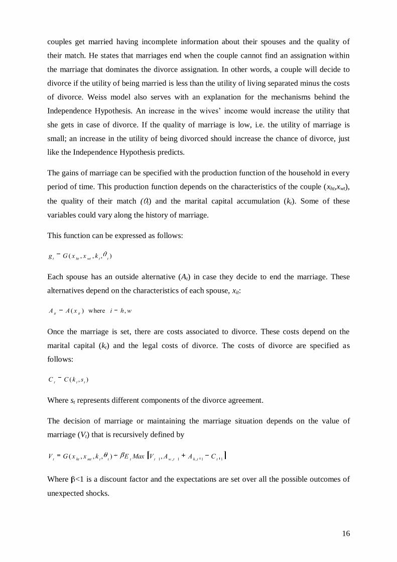
The decision of marriage or maintaining the marriage situation depends on the value of

marriage (Vt) that is recursively defined by

Vt

G ( xht

, xmt

, kt,

t) E

tMax V

t 1, A

w , t 1A

h , t 1C

t 1

Where <1 is a discount factor and the expectations are set over all the possible outcomes of

unexpected shocks.

17

Then, every period, the couple will decide to stay married if the value of marriage exceeds the

sum of the outside opportunities and will get divorced otherwise.

Vt( x

ht, x

mt, k

t,

t) A

wtA

htC

t

The empirical investigation will be framed on the Weiss model. Each of the variables that will

be studied will have relation to either the value of the marriage, Vt, the outside option of the

spouses, Ait, or the costs of divorce, Ct. The hypothesis of this investigation will depend on

how our observable variables affect the utility of marriage, Vt, the outside option, Ait, and the

costs of divorce, Ct.

The insertion of the divorce law in Chile, specifically the inclusion of the law that states that

the divorced wives should be economically compensated in case they ceased to work during

their marriage, should increase the utility of divorce provoking an increase in the probability

of divorce. This means that, under this theoretical framework and similarly to the other

theoretical models, the economic compensation should work in the same way that wives‟

income when increasing the utility of divorce.

Hypothesis

As it was explained above, Chile might be perceived as a relatively conservative country. This

implies that the belief in gender traditionalism and hence the idea that within marriage the

wife and the husband have fixed responsibilities, the former as the provider and the latter as

the housewife, still prevails. The Chilean survey “Voz de Mujer” (Women‟s Voice, 2005)

shows that 61,8 percent of women say that they are the ones in charge of the education and

caring of the children. Moreover, 42,1 percent of the men say that the education and caring is

their couple‟s obligation, because they are in charge of the exercise of authority and

recreation of the children. In relation to the housework routine, 78,3 percent of the women

and 63,9 percent of men say that the general housework, cooking, washing and cleaning is a

women‟s responsibility13

. Evidently, gender traditionalistic attitudes vary throughout the

Chilean society; nevertheless as an aggregate it should have an effect on the outcome of the

investigation. As wives start working and helping out the husbands providing the families it

should be expected that the husbands also start participating in the housework, in order to

maintain the equilibrium in the household‟s division of labour. Considering that the Chilean

society remains very traditional it is likely that the wives perceive household division of

labour as inequitable. This could provoke that the wives‟ perception of marriage decreases

13 “Mujer, Trabajo y Familia: Hacia una Nueva Realidad”, based on the Survey Voz de Mujer (2005), by

Comunidad Mujer.

18

and so does the perceived utility of being married. On the other hand, the economic

independence of wives provides them with the resources to leave those marriages in case they

want to.

In terms of the four perspectives explained above it is likely that, due to the general

characteristics of the Chilean household, the outcome of this investigation approaches the first

perspective. Oppenheimer (1997) states that the positive correlation between wives‟ income

and divorce is based on the Independence Hypothesis, which, in turn, is based on traditional

gender specialization. Since Chile is a country where conventional gender specialization still

prevails, I expect a positive correlation between wives‟ income and probability of divorce.

However, studies from the US, Sweden and Finland (Kesselring et al. 2006, Liu and Vikat,

2004, and Jalovaara, 2003) have had similar results, showing that if the female‟s earnings

become an important proportion of the total family income, the likelihood of divorce

increases even without fixed gender roles. This means that in Scandinavian counties an

increase in wives‟ income relative to their husbands‟ income, i.e. an increase in wives‟

income keeping total household income fixed, has a positive effect on the odds of divorce.

These results contradict what Oppenheimer says because Scandinavian countries usually

stand for egalitarian gender attitudes and these results support the Independence Hypothesis.

I will measure wives‟ economic situation by a level variable – wives‟ total monthly earnings -

and by a ratio variable – wives‟ income as a percentage of total household income. Thereby, I

will be able to test the hypothesis through a „level‟ and a „ratio‟ perspect ive. The level

variable would then represent wives‟ outside option or utility in case of divorce. On the other

hand, the ratio variable would reflect the difference or proportion between the economic

utility of divorce and the economic utility of marriage, where higher values would mean that,

ceteris paribus, the economic gains of marriage are more than the gains from divorce divorce.

In a way, both measures of wives‟ earnings serve to prove the Independence Hypothesis,

nevertheless they differ on the mechanisms that underlie it: wives‟ income reflects the quality

of the outside optionwhile wives‟ percentage income reflects the comparison of the utility of

marriage and divorce.

Since total household income is equivalent to wives‟ income (Ywife) divided by wives‟

percentage of income (%Ywife), the effect of household income is implicit in the model.

The Independence Hypothesis and the mechanisms that underlie it are based on the wife and

her decision to get divorced. These theories simplify marriage and do not analyse how a

change in wives‟ income could affect the husband‟s preferences for divorce. This argument

19

would not be an issue if we had information about which of the spouses made the decision to

get divorced in each of the cases14

. However, the data used in this investigation does not

specify whether the wife or the husband decided to end the marriage. Moreover it just shows

if a couple that was married in period t-1, is still married, divorced or separated in period t.

This means that among the divorced couples there are a percentage of dissolutions where the

husband made the decision, and another percentage where the wife was the one to decide to

break up. Nonetheless, this specific investigation can still be useful to assess whether the

effect that wives‟ income has on divorce is due to the Independence Hypothesis, given a

couple of additional assumptions.

It is likely that an increase in wives‟ income has an effect on the husband‟s preferences

regarding marriage and divorce. An increase in wives‟ income could awaken a feeling of

inferiority or insecurity in the husband because of the traditional gender role that sets the

husband as the main provider of the family. Furthermore, an increase in wives‟ income could

make the husband feel less responsible for his wife and children in case of divorce, both

reasons that could make the husband more prone to finish the marriage. If these where the

causes that make the husband more prone to terminate the marriage, the separation would still

be associated to the wife‟s independence, so it can be regarded as supporting evidence of the

Independence Hypothesis.

As explained above, the „divorce‟ observations include divorces driven by the wife and

divorces driven by the husband. Since we expect an increase in wives‟ income to increase the

chances of divorce in both cases, it is highly probable that the overall effect of an increase in

wives‟ income is positive, nevertheless it is possible that the positive effect is not only due to

the Independence Hypothesis. Moreover, it is impossible to know if an increase in wives‟

income made the wife, the husband or both spouses more prone to divorce. We just observe if

the probability of divorce of the couple increases when wives‟ income increases.

Despite all this, in the text I explain that finding a positive effect of wives‟ income on divorce

would be an argument in favour of the Independence Hypothesis. Yet it is important to

acknowledge that the positive correlation between wives‟ income and the probability of

divorce could be overestimated because of some „husbands‟ effects‟ that are not included in

the stylized model. On the other hand, the main focus of this investigation is to make an

empirical study of the effect of wives‟ income on the probability of divorce, regardless of

14 The onlz paper in the literature that incorpores this information to the analysis is Roggers (2004)

20

what spouse was the one to make the decision of divorce. In this regard, the proof of what

drives the Independence Hypothesis is only secondary to the analysis.

Hypothesis on the Effect of the Divorce Law

The divorce law of 200415

states that in case of divorce the stronger spouse has to compensate

the other one for the time he or she did not work in order to take care of the children or do the

housework. The economic compensation depends positively on, (a) education and age,

because the relation of these variables with the income that the wife would have earned if she

would have worked; (b) years married, because it is correlated to the amount of time the wife

dedicated to the family, and, (c) on the economic situation of the husband (or strongest

spouse) and his capability of paying that compensation. This should provoke that a non-

working housewife that has a vast education, has been married for a long time and has a rich

husband can easily make the decision to get divorced, even if she does not have personal

assets, because her compensation will be considerable.

The expected effect of the divorce law on the outcomes of this investigation is not simple.

Firstly, the economic compensation that the non-working wife will receive after divorce

should make wives‟ economic independence less important for the decision of divorce,

because if she did not work she will be compensated for that. Yet, it is also expected that the

smaller, yet still positive, effect of wives‟ income on the likelihood of divorce should be

counterbalanced by a bigger effect of age (directly and as a proxy of years married16

),

education and total household income on the chance of divorce so that I cannot predict if the

actual rate of marital dissolution would increase or decrease. I expect that in the regression of

the first period, that covers the years where there was no divorce law, the effect of wives‟

income is bigger than in the second regression. The divorce law should also provoke positive

changes in the coefficients of age and education, where it is expected to have bigger

coefficients in the regression that covers the years where the divorce law has been effective.

The change in these coefficients is due to the fact that the compensation depends on those

variables and since the compensation increases the outside option of the wives, these variables

will also increase it. The effect of the divorce law can also be observed through the variable

%Ywife, because it is negatively correlated to the amount of the compensation. Since the

compensation is greater when the household‟s income is bigger, the expected effect of

%Ywife on the odds of divorce in the second period is unclear: On the one hand, it should be

smaller because it is less necessary to have economic independence in case of divorce because

15 Shown in the Appendix. 16 The variable years married is not available in the database.

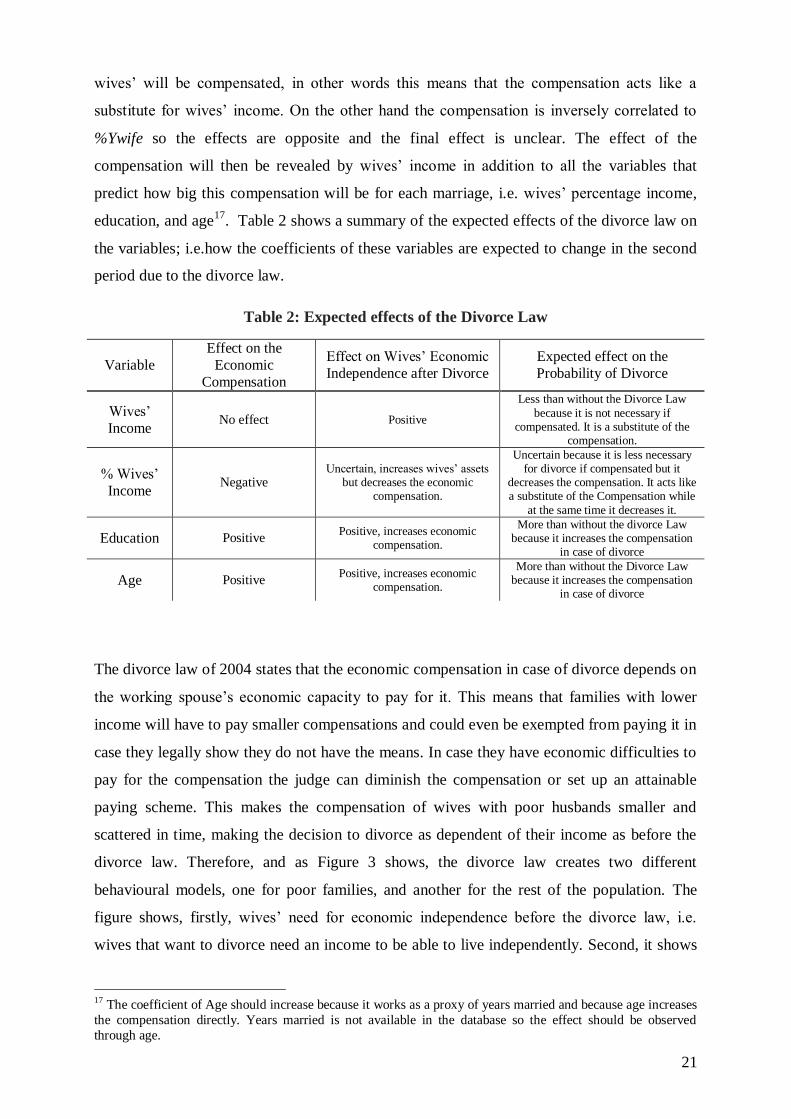
21

wives‟ will be compensated, in other words this means that the compensation acts like a

substitute for wives‟ income. On the other hand the compensation is inversely correlated to

%Ywife so the effects are opposite and the final effect is unclear. The effect of the

compensation will then be revealed by wives‟ income in addition to all the variables that

predict how big this compensation will be for each marriage, i.e. wives‟ percentage income,

education, and age17

. Table 2 shows a summary of the expected effects of the divorce law on

the variables; i.e.how the coefficients of these variables are expected to change in the second

period due to the divorce law.

Table 2: Expected effects of the Divorce Law

Variable

Effect on the

Economic

Compensation

Effect on Wives‟ Economic

Independence after Divorce

Expected effect on the

Probability of Divorce

Wives‟

Income No effect Positive

Less than without the Divorce Law

because it is not necessary if compensated. It is a substitute of the

compensation.

% Wives‟

Income Negative

Uncertain, increases wives‟ assets but decreases the economic

compensation.

Uncertain because it is less necessary for divorce if compensated but it

decreases the compensation. It acts like a substitute of the Compensation while

at the same time it decreases it.

Education Positive Positive, increases economic

compensation.

More than without the divorce Law because it increases the compensation

in case of divorce

Age Positive Positive, increases economic

compensation.

More than without the Divorce Law because it increases the compensation

in case of divorce

The divorce law of 2004 states that the economic compensation in case of divorce depends on

the working spouse‟s economic capacity to pay for it. This means that families with lower

income will have to pay smaller compensations and could even be exempted from paying it in

case they legally show they do not have the means. In case they have economic difficulties to

pay for the compensation the judge can diminish the compensation or set up an attainable

paying scheme. This makes the compensation of wives with poor husbands smaller and

scattered in time, making the decision to divorce as dependent of their income as before the

divorce law. Therefore, and as Figure 3 shows, the divorce law creates two different

behavioural models, one for poor families, and another for the rest of the population. The

figure shows, firstly, wives‟ need for economic independence before the divorce law, i.e.

wives that want to divorce need an income to be able to live independently. Second, it shows

17 The coefficient of Age should increase because it works as a proxy of years married and because age increases

the compensation directly. Years married is not available in the database so the effect should be observed

through age.

22

how this dependency changes after the law. The situation changes with the inclusion of the

divorce law because the economic compensation serves as a substitute for wives‟ income,

nevertheless the economic compensation (that also depends on age, years married and

education) is only considerable for wives with relatively rich husbands. The situation does not

change for wives with poor husbands; therefore the divorce law should not have an effect on

them.

In sum, the divorce law acts like an external shock in the investigation that introduces another

source of economic independence for divorced women: The Economic Compensation.

5 Empirical Approach

The empirical investigation is based on Weiss‟ Model (1997). Weiss states that if the utility of

marriage is more than the utility of getting divorced, i.e. , the

couple will continue to be married, otherwise it will get divorced. For simplicity the left part

of the equation above will be called Mt representing the utility of being married. The right part

of Weiss‟ equation will be called Dt and it will represent the utility of divorce. The probability

of divorce, Yt, will depend on Mt and Dt as latent variables and will be defined as follows:

Figure 3: Wives’ Behavioural Models regarding their need of Economic

Independence to get a Divorce before and after the Divorce Law

23

Mt and Dt are unobservable latent variables while the act of divorce can be observed.

Furthermore, we know what variables affect Mt and Dt so this investigation will study those

variables and test how they affect our observable variable Yt.

This investigation will focus on couples that are confronted to the decision of maintaining

their marriage or end it. Since each wife carries the information of their family (total income,

number of children, if they own a house, etc.) the nucleus of this study will be the wives,

because including the husbands would generate a duplication of the information. Then, each

observation is a woman, which includes information of her family and husband. I will study

the impact of wives‟ economic independence on the conditional probability of getting

divorced in time interval t, given that the couple has not separated until the beginning of

period t. Economic independence will be measured in two different ways: As wives‟ income

capacity and as wives‟ share of the household‟s total income.

The main potential problem of this estimation is the endogeneity of wives‟ income, i.e. wives‟

monthly total income, which includes their wage and other sources of income. Johnson and

Skinner (1986) find that married women react to high odds of marital disruption by increasing

their labour supply. This endogeneity problem could bias the estimates by overestimating the

real effect of wives‟ income on divorce, so it must be corrected. I will use a two-step

estimation method using Instrumental Variables in order to reduce this problem. Burgess et al.

(2003) correct this problem by using the average earnings rate and stripping out the year-to-

year changes in income. They also try to correct the endogeneity by estimating a long run

fixed effect measure of wage rates and income. Booth et al. (1984), on the other hand, try to

correct this problem through a recursive structural equations model where they divide the

independent variables between intervening variables and control variables. The authors

identify each variable in the model through separate equations and the intervening variables

are added to successive equations in a specific order, starting up with the amount of hours a

wife works, because it is the only variable in the model that can be explained only by

exogenous variables. Nunley (2007) studies the effect of household income volatility on

divorce. He also corrects for the simultaneous relationship between household income and the

risk of divorce by using instrumental variables to run an OLS estimation of household income

volatility. He estimates income volatility through several instruments like occupation

24

indicators, individual labour-market characteristics and country-level variables including

education, type of employment and other individual characteristics.

A second potential problem is the selection bias caused by using only married couples. It is

important to note that the decision of divorce depends on the decision of marriage, and both

decisions depend on income. If the study only focuses on married couples the results will not

be accurate because there would be a selection bias. Thus, single women will be considered in

this study as well. The decision of marriage is affected by the economic situation of the

spouses so this has an effect on the decision of divorce. The literature about the decision to

get married indicates that women‟s income is negatively correlated to this decision (Burgess

et al., 2003). Accordingly, married women as an aggregate should have less economic assets

or income than single women. This should introduce selection bias to this investigation if it

only considers married women in the sample.

Single women do not divorce, but if they would get married they would have to make that

kind of decisions. The decision to get divorced implies the decision to get married in the first

place. For this reason, and to correct for a potential selection bias, I will use a specific version

of the Heckman correction model for binary representations proposed by Van de Ven and Van

Praag (1981).

5.1 Empirical Model and Method of Analysis

The idea is to study the relationship between wives‟ income and the probability of divorce

through a probit regression estimating the chance of divorce between 1996 and 2001, subject

to the initial information of 1996. Next, I repeat the same but for the period between 2001 and

2006 using information of 2001. With these two regressions I should be able to investigate

whether the wives‟ income affects the marriage stability and if the divorce law of 2004 had

any effect on that outcome. The equation to be estimated for each period of time is:

P (Y 1 | z) (Z )

With ,

Z0 1

Ywifej 2

%Ywifej 3

Cj

Where Ywifej is wives‟ income, %Ywifej is the wives‟ income as a percentage of total

household income and Cj are the control variables that will be explained in detail in the next

section.

In this study I will deal with the potential endogeneity of wives‟ income through instrumental

variables following the method used by Nunley (2007). The variables “Wives‟ Income” and

25

“Wives‟ Income as a Percentage of Total Household Income” are potentially endogenous. A

simple method of instrumental variables for binary response models will intend to solve the

endogeneity problem. Consequently, the final model will include the residuals of the

estimations of these variables (the residuals of the first stage regressions) together with the

potentially endogenous variables, following the IV method for probit. The estimation of the

wives‟ income will depend on various dummy variables regarding the type of employment of

the wife, i.e. if she works independently, as a public or private employee, as a domestic

employee, as a boss, works in the family without remuneration, or in the armed forces. These

are variables that are correlated to income but are irrelevant for the decision of divorce; hence

they should work as instruments. Nunley (2007) uses type of job as an instrument, so he

includes dummies for doctors, lawyers, gardeners, and other occupations. The database used

in this investigation does not have such information. However, it has the type or level of

employment which is information that is not directly related to the decision of divorce yet it

relates to it only indirectly through income.

The first stage estimation of wives‟ percentage of income (%Ywife) will include the education

of the husband‟s parents and regional dummies because these are variables that predict

%Ywife but are irrelevant for the decision of divorce.

The first-step equations and specification of the instruments will be estimated through OLS

and the residuals of these estimations, together with the potentially endogenous variables, will

be added to the final divorce equation so that the income variable is no longer correlated to

the error term. Wives‟ income (Eq. 1) and wives‟ percentage of income (Eq. 2) will be

estimated as shown below.

Ywifej 0 1

Wj 2

Pj 3

Cj

v1 (1)

%Ywifej 4 5

Wj 6

Pj 7

Cj

v2 (2)

Where Wj are the instruments for wives‟ income which are a set of dummies regarding the

type of employment of the wife; Pj are the instruments for %Ywife which are the husband‟s

parents‟ education and the region of Chile where they live, and Cj are all the control variables

in the divorce equation.

The method of instrumental variables in binary response models is not as straightforward as in

linear models. Instead of including the predictions of the first stage regressions I include the

residuals of it, together with the variables as such (not predicted) as shown below. The

method works as follows: (a) Run an OLS regression of equations (1) and (2) and save the

26

residuals ˆ v 1 and ˆ v

2. Then (b) run the Probit of the probability of divorce on the potentially

endogenous variables, the control variables and the residuals of the first stage regressions

(Ywife, %Ywife, C, ˆ v 1 and ˆ v

2) (Wooldridge, 2001). The probit with the instrumental variables

method will then be,

P (Y 1 | z) (Z )

With ,

Z0 1

Ywifej 2

%Ywifej 1

ˆ v 1 2

ˆ v 2 3

Cj

(3)

With this method I will get consistent estimators of the scaled coefficients 1,

2,

1, and

2.

The usual probit t-statistic on ˆ v 1 and ˆ v

2 is a valid test of the null hypothesis that Ywife and

%Ywife are exogenous. There are two possibilities why 1 or

2 are not statistically

significant. First, their corresponding variable is exogenous to the model and in this case their

corresponding coefficients are correct (not scaled) and consistent. Second, their corresponding

variable is endogenous and instruments are not adequate. If the variables turn out to be

endogenous, this method makes the estimators consistent but scaled so they need to be

transformed (divided by ( ˆ 2ˆ

21)

1 / 2, where ˆ is the coefficient of the residuals of the first

stage regression - ˆ v 1 or ˆ v

2- in the second stage regression‟s outcome, and ˆ

2 is the variance of

ˆ v 1 or ˆ v

2, depending on the case) to get the real consistent estimators of the coefficients.

Heckman Correction for Binary Models (Van de Ven and Van Praag, 1981)

The Heckman correction method is a two-step statistical approach that intends to correct for

non-randomly selected samples. The method is relatively easy to implement and has a firm

basis in statistical theory. It is based on a two-stage estimation method to correct the selection

bias. There is an adaptation of the Heckman selection model for binary choice models

proposed by Van de Ven and Van Praag (1981) that will be very useful for this investigation.

This adaptation is very similar, though rarely used because it is more difficult to implement

computationally than the linear version (Dubin and Rivers, 1989). This method is

conceptually straightforward; it starts by specifying a selection model, in this case the

probability of being married, that results in a bivariate model which, in turn, can be estimated

by maximum likelihood. Two assumptions must be made in order to estimate with maximum

likelihood: First, all the explanatory variables are exogenously determined, and second, that

the observations must be independently and identically distributed, i.e. that the observations

were selected randomly from some population.

27

Before implementing the model it is important to acknowledge its flaws and check if these

disadvantages are important for the investigation. The two-step estimation of the Heckman

correction method assumes that the errors are jointly normal. In the case they are not normal

the estimators could be inconsistent and lead to erroneous conclusions in small samples

Puhani (2000). Puhani also states that in most cases, an exclusion restriction is required to

generate credible estimates. There must be at least one variable in the selection model that is

exogenous to the equation of interest. If no such variable is available, it might be difficult to

correct the sample selection bias. In this case, the variable that should appear with a non-zero

coefficient in the selection equation and that is exogenous to the divorce equation will be

“being more than 18 years old”. In Chile, people cannot get married until they are 18 years

old18

. If they wish to get married before that they need their parents‟ approval. Therefore,

being older than 18 is a variable that is pertinent to the marriage model but not to the divorce

model and for this reason it should work as the exclusion restriction.

5.2 Data, Variable Description and Expected Results

The database that will be used is the Panel Casen (1996, 2001, 2006). This database covers

the regions III, VII, VIII and the Metropolitan Region of Chile. The idea of using a panel data

set is that it increases the accuracy of the study because it provides information about the

timing when the couple divorces, even though the method of investigation is cross section.

Variable Description

Dependent Variable:

Divorce (Y): The dependent variable in this investigation is the probability of getting

divorced, this is, the probability that Y=1. If a couple is married in period t and then is

divorced, annulated or separated in t+1, then Y=1; if the couple that is married in t is still

married in t+1, Y=0. The probability of divorce then is P(Y=1). By “t” it is meant the

beginning of the observed period. The time index “t” will be 1996 in the first period

regressions and 2001 in the second period regressions. Consequently, “t+1” will be 2001 in

the first regressions and 2006 in the second ones.

Explanatory Variables:

We will measure wives‟ income in two different ways to have more accurate results. There

are hypotheses based on wives‟ income measured as actual income (money) and others based

on wives‟ economic situation measured as a percentage of the total household income. The

18 Law 19585, Art. 1º Nº 13

28

proposition of this investigation is to test the „Independence Hypothesis‟ that is based on

wives‟ income. Nevertheless, our study will be complemented by adding wives‟ income as a

percentage of total income as another explanatory variable. Adding wives‟ percentage income

to the study will enable us to compare the level effect (economic independence) and the ratio

effect (inverse of the gains from marriage respect to the outside option) leading the study to

more precise conclusions.

Income Wife (Ywife): Wives‟ income reflects the total income of the wife in period t. It

includes labour income and income from other sources such as rent. The wives‟ income

represents the economic independence of the wife, regardless of the fact whether she works or

not. For this reason not only labour income was included, but instead, all sources of income

were incorporated. In order to be able to compare the results in both periods of time, the

income of both periods is measured in prices of 1996 so the effect of inflation is corrected.

The variable that explains if the wife works or not was not included as a control variable in

the regression because such information is almost perfectly contained in Ywife, in other

words, almost all wives with income are working (the correlation between work income and

total income is 0.86).

Percentage Income Wife (%Ywife): The wives‟ income as a percentage of the total household

income is constructed as the total income of the wife (Ywife) divided by the total household

income. This version of wives‟ economic situation reflects an inverse of the relative gains

from marriage with respect to the outside option, where a low percentage would mean that the

husband supports the wife economically. Values between 40% and 60% would mean that the

household economy depends more or less equally on both spouses and high values of this

variable should reflect that the wife is the main provider of the household.

The regressions will include Ywife and %Ywife at the same time so the variable “Total

Household Income” must not be included in the model.

%YwifeYwife

Yhousehold

As shown above, total household income cannot be included in the model because it would

create perfect collinearity. Nevertheless, since total household income (Yhousehold) is a

combination of %Ywife and Ywife, the information that this variable provides is implicit in the

model.

Control Variables, Ct:

29

Economic Hardship (EconHardship): This variable is defined as the amount of times one

member of the family has been unemployed between t and t+1. For the first period‟s

regression this is between 1996 and 2001 and for the second period, between 2001 and 2006.

It is important to acknowledge that, due to differences in the survey, Economic Hardship in

the first period is measured in a different way than in the second period . For the first period it

is measured as the amount of times somebody in the family was unemployed whereas in the

second period it is the amount of people in the family that where unemployed at least once in

that period. This variable is important because it could be correlated to the decision of getting

divorced and to economic matters.

Age of the wife (AgeW): AgeW is the age of the wife in period t. The age of the wife is an

explanatory variable in the marriage model and in the divorce model. It is important because

it is correlated to income and to the divorce decision.

Number of children under 9 (nChild9): This variable shows the amount of children under 9

years old that are part of the households and live there. The number of children in the family

affects the decision to work so it is correlated to income and it also affects the decision to end

the marriage so it must be included in the model.

Owning a house (House): House is a dummy variable, which is 1 in case the couple owns the

house and 0 otherwise. Owning a house increases the costs of divorce and is also correlated to

income so it has to be a control variable.

Education wife (educW): Education wife is the amount of years of education that the wife

had. Wives‟ education works as an explanatory variable in the divorce equation and in the

marriage selection equation. We will also add dummies to check if having a university degree

or a technical degree affects the probability of divorce (and marriage) besides the number of

years studied.

Education husband (educH): The education of the husband is the number of years of

education that the husband has. Husbands‟ education works as a control variable in the

divorce equation.

Being older than 17 (more18): This is a dummy variable that is 1 if the person is 18 years old

or older and 0 otherwise. It is a crucial variable in the sample selection equation because it is

relevant to the decision of getting married but irrelevant to the decision of getting a divorce.

30

Urban (Urban): Urban is a dummy variable that is 1 if the person lives in an urban area and 0

if she lives in a rural area.

Instrumental Variables:

Region: Region refers to different dummy variables regarding the region where the person

lives. There is one for the 3rd

region, for the Metropolitan region, for the 7th region and for the

8th region, nevertheless the 8

th region will be omitted in the model to prevent perfect

collinearity. Region serves as an instrumental variable (IV) for %Ywife because it predicts

%Ywife and it is irrelevant in the decision of divorce.

Education parents husband: The education of the parents of the husband will be a set of

dummy variables regarding the level of education that the father of the husband achieved.

This is, whether he has a university degree, a technical degree or high school degree, and the

excluded segment would be having less than a high school degree. This variable works as an

IV for %Ywife because it is correlated to the household total income (and hence to the wives‟

percentage of total income) and it is exogenous to the decision of divorce.

Type of Employment of the Wife: Type of employment of the wife refers to several dummy

variables that show the different type of employment of the wife. This could be that she works

as a boss, independently, as a public or private employee, as a domestic employee19

, in the

armed force or works in the family without remuneration. The type of employment that a

women has, clearly explains her wage, nevertheless it has nothing to do with the decision of

divorce and hence serves as an instrument for wives‟ income. The excluded dummy is “not

working”.

Expected effects of the variables

Following Weiss‟ model, a couple will divorce if the utility of being divorced is higher than

the utility of remaining married. Before analysing how each variable should affect the chance

of divorce it is important to check how each variable affects the utility of marriage and the

utility of divorce. This investigation will be based on the study of the observed variables,

specifically the ones regarding the income of the wife, and how these variables make divorce

more or less likely. Beneath there is a summary of the expected effects of each variable on the

utility of marriage and divorce.

19 Working as a domestic employee in Chile is to work in a private house, mainly as a cook, a maid or a nanny.

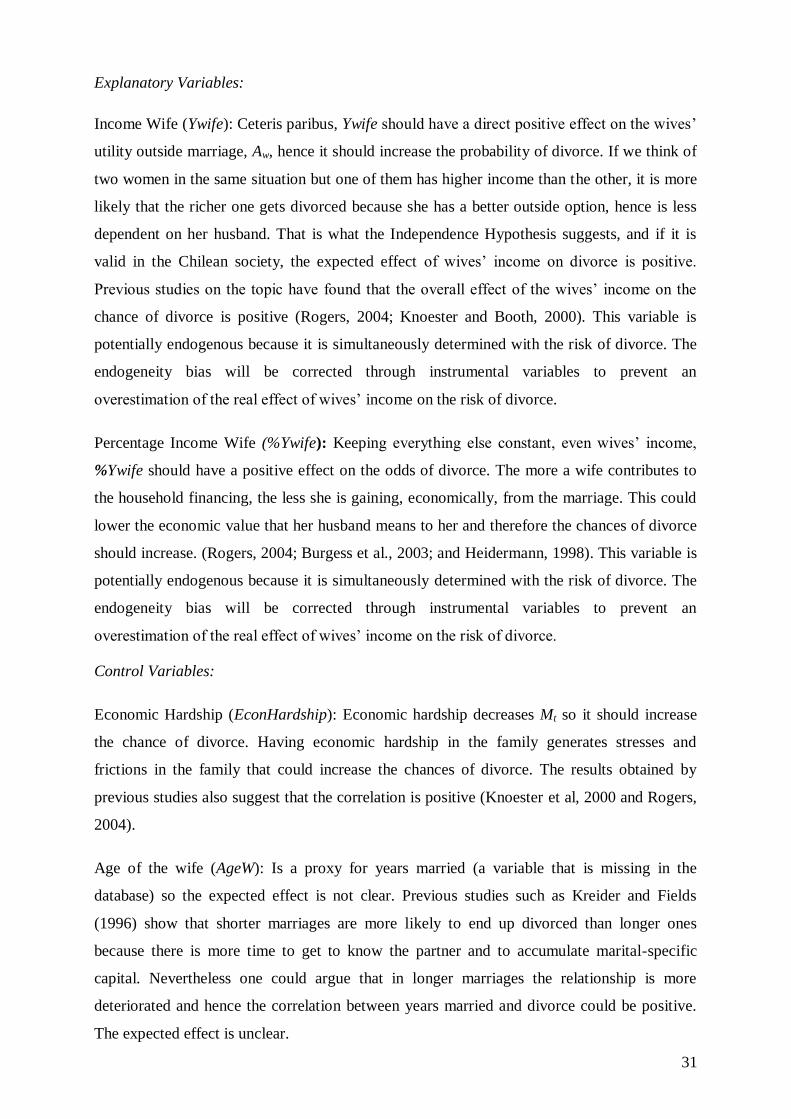
31

Explanatory Variables:

Income Wife (Ywife): Ceteris paribus, Ywife should have a direct positive effect on the wives‟

utility outside marriage, Aw, hence it should increase the probability of divorce. If we think of

two women in the same situation but one of them has higher income than the other, it is more

likely that the richer one gets divorced because she has a better outside option, hence is less

dependent on her husband. That is what the Independence Hypothesis suggests, and if it is

valid in the Chilean society, the expected effect of wives‟ income on divorce is positive.

Previous studies on the topic have found that the overall effect of the wives‟ income on the

chance of divorce is positive (Rogers, 2004; Knoester and Booth, 2000). This variable is

potentially endogenous because it is simultaneously determined with the risk of divorce. The

endogeneity bias will be corrected through instrumental variables to prevent an

overestimation of the real effect of wives‟ income on the risk of divorce.

Percentage Income Wife (%Ywife): Keeping everything else constant, even wives‟ income,

%Ywife should have a positive effect on the odds of divorce. The more a wife contributes to

the household financing, the less she is gaining, economically, from the marriage. This could

lower the economic value that her husband means to her and therefore the chances of divorce

should increase. (Rogers, 2004; Burgess et al., 2003; and Heidermann, 1998). This variable is

potentially endogenous because it is simultaneously determined with the risk of divorce. The

endogeneity bias will be corrected through instrumental variables to prevent an

overestimation of the real effect of wives‟ income on the risk of divorce.

Control Variables:

Economic Hardship (EconHardship): Economic hardship decreases Mt so it should increase

the chance of divorce. Having economic hardship in the family generates stresses and

frictions in the family that could increase the chances of divorce. The results obtained by

previous studies also suggest that the correlation is positive (Knoester et al, 2000 and Rogers,

2004).

Age of the wife (AgeW): Is a proxy for years married (a variable that is missing in the

database) so the expected effect is not clear. Previous studies such as Kreider and Fields

(1996) show that shorter marriages are more likely to end up divorced than longer ones

because there is more time to get to know the partner and to accumulate marital-specific

capital. Nevertheless one could argue that in longer marriages the relationship is more

deteriorated and hence the correlation between years married and divorce could be positive.

The expected effect is unclear.

32

Number of children under 9 (nChild9): Has a direct effect on Mt (the utility of being married)

and Ct (costs of divorce) so it should decrease the chance of divorce. Previous literature on the

subject also finds a negative correlation between the number of children under 9 and the

probability of divorce (Kraft et al., 2009; Rogers, 2004 and Burgess, 2003).

Owning a house (House): Owning a house increases the costs of divorce (Ct) so it should have

a positive effect on the utility of getting a divorce (Dt), and hence a negative effect on P(Y=1)

(Heidemann, 1998).

Education wife and Husband (educW and educH): One could argue that having a higher

education will facilitate people to find a good match and therefore the chances of divorce

should be less. On the other hand, having a good education could make people more critical

towards their marital life and increase the chances of divorce. The evidence from literature is

inconclusive. Kreider and Fields (1996) show that college graduates are more likely to marry

and less likely to divorce. On the other hand, Sanhueza et al. (2007) find a positive correlation

between education and marital disruption when studying Chilean couples. The overall

expected effect of education on the odds of divorce is unclear.

Being older than 17 (more18): This affects the probability of marriage but not the probability

of divorce so it is the variable that allows the use of the Heckman correction model. In Chile

it is compulsory to be older than 18 to get married20

, otherwise the consent of the parents is

needed. Consequently being older than 18 increases the chance of being married and does not

affect the probability of marital disruption.

Urban (Urban): Living in an urban area increases the chances of meeting a better match (after

marriage, because we do not have the information of where the couple lived before being

married) so it could have a positive effect on divorce. Sander (1985) finds that couples living

in an urban area are more likely to divorce than couples living in rural areas. They explain

this, in part, by the stronger sexual division of labour within the farm household, where, they

say, the gains from marriage are higher for farm housewives because they had acquired more

marital-specific capital, relative to their non-farm counterparts. The expected effect is

positive.

20 Law 19585 of the “Ley de Matrimonio Civil” (Law of civil matrimony)

33

Instrumental Variables:

Region: The effect of the region on %Ywife is not clear because it depends on the region but it

is likely that wives‟ living in the Metropolitan region of Chile have a higher percentage of

income than families of the 8th

region because of the higher accessibility of work for women,

in terms of transportation, supply of nursery places, kinder gardens, and female-job offers.

Women from the 3rd

region should have lower percentage of total household income than

women of the 8th

region because of the big amount of jobs for men relative to female jobs due

to the mining sector. The effect of living in the 7th

region should not be significant due to the

similarities of the 7th and 8

th regions. Anyhow, due to the speculative foundation of these

arguments and the lack of previous studies on the topic, the expected effect is unclear.

Education Parents husband: Having the wives‟ income fixed, the education of the husband‟s

parents should have a positive effect on the cultural level of the husband and hence it should

have a positive correlation to total household income. The expected effect of the husband‟s

parent‟s education on %Ywife is negative.

Type of Employment of the Wife: Each dummy variable should have a different effect. For

example, being a boss should have a positive effect on wives‟ income, being a private and

public employee should also be positive but less than being a boss. Working independently

could have a positive effect; nevertheless the magnitude of the effect is not clear because it

covers a wide range of different independent jobs (like being a gardener or having your own

company). Being a domestic employee21

could have a small positive effect because these

particular jobs are not very well paid in Chile. Working without remuneration in the family

should have a negative or no effect on wives´ income because it is an unpaid job so it should

not pay more than not working at all. All of these effects are relative to the excluded dummy

that is that the wife does not work at all.

In general, the idea is to run two probit regressions with Heckman correction for sample

selection, one for each period of time, first for the period between 1996 and 2001 before the

divorce law and then for the period between 2001 and 2006 after the divorce law. This should

enable us to compare the results and see if the law has an effect on the estimates of the

coefficients. Further, it is important to check for the different effects that the divorce law has

on rich and poor families because the economic compensation depends strongly on the

21 Working as a domestic employee in Chile means working in someone else‟s house mainly as a cook, a nanny

or a maid.

34

husband‟s capacity to pay for it. To test this, I will run a LPM22

with the same variables than

before including an interaction between the predicted wives‟ income and a dummy for

families that have an income over $500.00023

(around 1000 USD), Dhy, as a monthly income.

The idea of using the interaction variable is to check if the divorce law affects everybody or

only the part of the population that is able to afford the economic compensation in case they

finish their marriage.

It is expected to have a linear positive relation between both measures of wives‟ income and

divorce, i.e. between Ywife and %Ywife and P(Y=1|Z). If the results turn out as expected, the

partial effect of Ywife on P(Y=1|Z) should be positive and the partial effect of %Ywife on

P(Y=1|Z) should be positive as well. Regarding the interaction variables it is expected to have

a non-significant effect in the first period because I expect high and low income families to

behave equally. In the second period it is expected to have a negative effect, i.e. I expect

couples with higher income to behave significantly different than couples with relatively

lower income. In summary, the equations to be estimated for each period will be

Ywifej 0 1

Wj 2

Pj 3

Cj

v1 (1)

%Ywifej 4 5

Wj 6

Pj 7

Cj

v2 (2)

P (Y 1 | z) (Z )

With ,

Z0 1

Ywifej 2

%Ywifej 1

ˆ v 1 2

ˆ v 2 3

Cj

(3)

And, to test the difference in behaviour,

P (Y 1 | z)0 1

YwifePj 2

%YwifePj 3

YwifePj* Dhy

j 4C

j (4)

Where YwifePj and %YwifePj are the predictions of Ywifej and %Ywifej, estimated by Eq. 1

and Eq.2.

The expected effects of the variables for each period are summarized in Table 3.

22 To test the difference in behaviour it is necessary to add an interaction of the predicted variable Ywife with a

dummy, so for simplicity reasons this specification will be estimated through a LPM instead of a Probit. 23 $500.000 today, which is equivalent to $300.000 of 1996

35

Table 3: Expected Effects of the Variables before and after the Divorce Law

Variable Expected Effect

Before the Law

Expected Effect

After the Law Change

Ywife + + -

%Ywife + + +/-

YWife*Dhy 0 - -

nChild9 - - No

EducW +/- + +

EducH +/- +/- No

EconHard + + No

AgeW +/- + +

House - - No

Urban + + No

6 Results

The descriptive statistics of the main variables are shown below, in table 424

.

It is interesting to see that the divorce rate in both periods is relatively small compared to

what is shown by the national data (INE): This survey shows that up to 1998 more than half

of the marriages end up separated or annulated. Clearly, that data includes the lifetime of

marriages and hence must be greater than the chance of getting a divorce in a period of 5

years, however the 1% rate makes us believe that this particular sample shows fewer marital

disruptions than the national statistics. The low number of divorces in the sample could cause

efficiency problems in the estimations; yet, if the independent variables‟ variance is

sufficiently big, the efficiency problem might not be so critical for the estimations. A

considerable variance of the independent variables within the divorced couples enhances the

reliability of the estimations. The variance of wives‟ income within the cases of divorce

(when Y=1) is considerable (see Table E1 and E2 in the Appendix) so the low amount of

divorces should not affect significantly the efficiency of the estimations.

Table B1a and B1b (in the Appendix) show the outcome of the first stage regression for

wives‟ and total household‟s income. These results correspond to the outcome of the

estimation of equations (1) and (2) for each period of time and will be used in the subsequent

estimations to solve the potential endogeneity problem. As expected, the type of employment

that wives have affects their income, relative to the excluded category that is not working. All

types of employment have positive effects on income because they provide more than not

working, except for “working for the family without remuneration”. Being a boss is the most

profitable type of employment, followed by being a public employee, being a private

employee, working in the armed force, independently and as a domestic employee. As

24 In table A1 of the appendix there is bigger table with the descriptive statistics.

Table 4: Descriptive Statistics of Main Variables

37

expected, working (unpaid) for their families has a negative yet not significant effect on

wives‟ income because they are not remunerated for their jobs. This result is reasonable

because there should not be a significant difference on the income of nonworking wives and

wives that work without remuneration. All the rest of the employment category dummies are

statistically significant from zero for both periods of time and do not affect the decision of

divorce so should serve as instruments for wives‟ income. Not every instrument proposed to

estimate wives‟ income as a percentage of total household income shows to be significant.

Interestingly the husbands‟ parents‟ education does not affect significantly %Ywife. The only

dummy regarding the parents‟ education that appears to affect significantly %Ywife is if the

husband‟s father had a high school degree, where the effect appears to be negative in relation

to the excluded category (that is if the husband‟s father had less than a high school degree) yet

only significant for year 2001. Since the parent‟s education does not serve as an instrument

for %Ywife, the regional dummies need to be significant in order to proceed with the IV

method. The regional dummies are proper instruments for %Ywife because they appear to

have statistically significant effects on %Ywife and do not affect the decision of divorce.

Specifically, living in the 3rd

, 7th, or Metropolitan (13

th) region of Chile affects negatively

wives‟ income as a percentage of total household income, relative to living in the 8th

region.

The negative effect of living in the 3rd

or metropolitan region could be explained by the fact

that in those regions the husbands‟ income is relatively higher than in the 8th

region because

of the regional-specific productive industries, i.e. mining industry in the 3rd

region and

financial industry in the metropolitan region. The negative effect of the 7th region is difficult

to explain through the previous argument because both regions have similar businesses

(forestry, farming, fishing and livestock industries), nevertheless the 7th

region has less than

half of the 8th

region‟s manufacturing, commercial and service-oriented industries. In Chile,

most of the women work in these productive sectors so this could explain that wives‟ income,

as a percentage of household income, is higher when living in the 8th region than in the 7

th

region.

The residuals of these regressions were used in the estimation of the probability of divorce,

equation (3), together with Ywife, %Ywife and the control variables, following the IV

procedure for probit models. It is important to consider that, since the parents‟ education

dummies are not significant and the rest of the instruments are significant for both first stage

equations, the residuals that will be included in the second stage equation are likely to be

collinear. For this reason I report the outcomes of the second stage regression without the

residuals, with the residuals of each first stage equation separately, and with both residuals.

Comparing the outcomes of those four estimations we will be able to decide if the variables

38

are endogenous. The outcomes of all four models for both periods of time are shown in table

C1a and C1b in the appendix. Column 1.1, 1.2, and 1.3 show the outcome of the estimation of

the model without instrumentation. Columns 2.1, 2.2 and 2.3 are the outcomes of the

regression with the inclusion of both first-step equations‟ residuals. The last columns of tables

C1a and C1b show the estimations of the Probit with Heckman‟s correction method with one

of the variables instrumented, first Ywife and then %Ywife. From these last columns we

conclude that Ywife and %Ywife are endogenous in the first period and not in the second

period, even if the estimations of the model that includes both instrumented variables shows

that the residuals are not significant in neither of the periods. This, as explained above, could

be due to the collinearity between the residuals. In the second period (Table C1b) the

residuals are never significant so we can conclude that Ywife and %Ywife are not endogenous

between 2001 and 2006. Consequently, for the rest of the investigation we will not instrument

those variables in the second period in order to increase the efficiency of the estimation.

However, from the outcomes of the estimations of these four models for the first period

(Table C1a), we can conclude that there is enough evidence to say that both Ywife and %Ywife

are endogenous and need to be instrumented in order to have consistent estimations.

Regarding the selection equation, the excluded variable, being older than 17 years old, shows,

as expected, to have a positive and statistically significant effect on the decision to get

married. Considering this, the outcome of this regression also shows that rho is not

significantly different from zero in neither of the periods so, contrary to what expected, there

is no evidence of sample selection. For this reason, and in order to gain efficiency in the next

estimations, the next regressions will use a simpler model that does not correct for sample

selection.

Table 5: Marginal Effects, Endogeneity and Sample Selection Tests of Equation (3) with

Heckman Correction and IV

Variable Marginal Effect Endogeneity Sample

Selection

Income Wife 1996

9.40E-07 Yes No

% Income Wife 1996

-0.233 Yes No

Income Wife 2001

-1.59e-06 No No

% Income Wife 2001

0.356 No No

39

Table 5 shows a summary of the estimations of equation (3) using the Heckman Correction

model and including the residuals of equations (1) and (2) for the period where the variables

are endogenous. There is a positive correlation between wives‟ income and the probability o f

divorce. This result supports the Independence Hypotheses, nevertheless the marginal effect is

not statistically significant and that makes it difficult to tell if this result is conclusive. As

expected, this effect decreases with the inclusion of the divorce law. Differently, the effect of

wives‟ percentage of income is negative in the fist period and positive in the second period,

yet these results are not statistically significant either. It is important to acknowledge that the

reported results are the marginal effects, so the estimations shown illustrate the effect of a

change from 0 to 1 in %Ywife on the probability of divorce, this is, the difference between

paying for all the household expenses or not paying at all. The estimated effect of earning 1%

more of the total household income is then -0.0023 in the first period and 0.00356 in the

second period of study.

It is important to notice that given that the residuals of the fist stage equation do not have a

significant effect on the probability of divorce in the second period, i.e. neither Ywife nor

%Ywife shows to be endogenous in the second period; we do not need to transform the

estimations. However, in the first period both residuals are significantly different from zero.

This means that the marginal effects shown in Table 5 for the first period of time are based on

the estimations of scaled coefficients and they need to be transformed. The complete

regressions are shown in table C1a and C1b in the Appendix.

As explained above, the income variables are endogenous in the first period, therefore the rest

of the estimations will continue using the IV procedure on that period‟s estimations. On the

other hand, we will not follow the IV procedure when the variables are not endogenous

(second period) in order to increase the efficiency of the estimations. Moreover, considering

that there is not enough evidence of sample selection we will estimate equation (3) through a

probit model without Heckman‟s correction method. Table 6 shows a summary of the

marginal effects of wives‟ income on the probability of divorce using the method of

instrumental variables for the first period but not for the second one.

40

Table 6: Marginal Effects and Endogeneity Tests of Probit estimation of Equation (3)

with Instrumental Variables for the first period

Variable Marginal Effect Endogeneity

Income Wife 1996

1.34E-07 Yes

% Income Wife 1996

0.349 Yes

Income Wife 2001

-1.65e-06 -

% Income Wife 2001

0.480* -

The results regarding wives‟ income are, again, as expected. There is a positive effect of

wives‟ income on the odds of divorce. This effect decreases considerably in the second period

and becomes negative. In opposition to the previous results, yet as expected, wives‟

percentage of income has a positive effect on the probability of divorce in the period before

the Divorce law. This effect increases in the second period of time, supporting the results of

the prior regression. Both income variables show to be endogenous in the first period,

however, it is important to add that the marginal effects shown in Table 6 are based on the

real coefficients, i.e. they have already been scaled to be the real ones. The full outcomes of

these estimations are shown in tables C2a, and C2b in the Appendix. The last three columns

of table C2a show the estimations of the probit with IV for 1996-2001, where the first of these

three columns regards the divorce equation, and the other two are the first stage estimations.

Table C2b shows the full outcome of the Probit without IV for the period between 2001 and

2006.

Up to now, considering the outcomes of both specifications, the divorce law shows to

decrease the effect of wives‟ income in the decision of divorce and enhance the effect of

%Ywife. This means that when the divorce law is inserted, wives‟ aren‟t as dependent of their

income to get divorced, nevertheless they become more sensitive to an increase in %Ywife,

maybe because divorce appears to be more accessible. Also, both estimations show a positive

effect of Ywife on the odds of divorce yet the effect of %Ywife appears to be negative in the

first model and positive in the second model. The difference between the first specification

(probit with Heckman‟s correction method) and the second one (probit) is that the first one

includes married and non-married women in the sample whereas the second one only includes

wives. As stated above, rho is not statistically significant, which means that there is not

enough evidence to say that the sample was not randomly selected. However, this does not

mean that rho is null and therefore this could provoke differences in the estimation of the

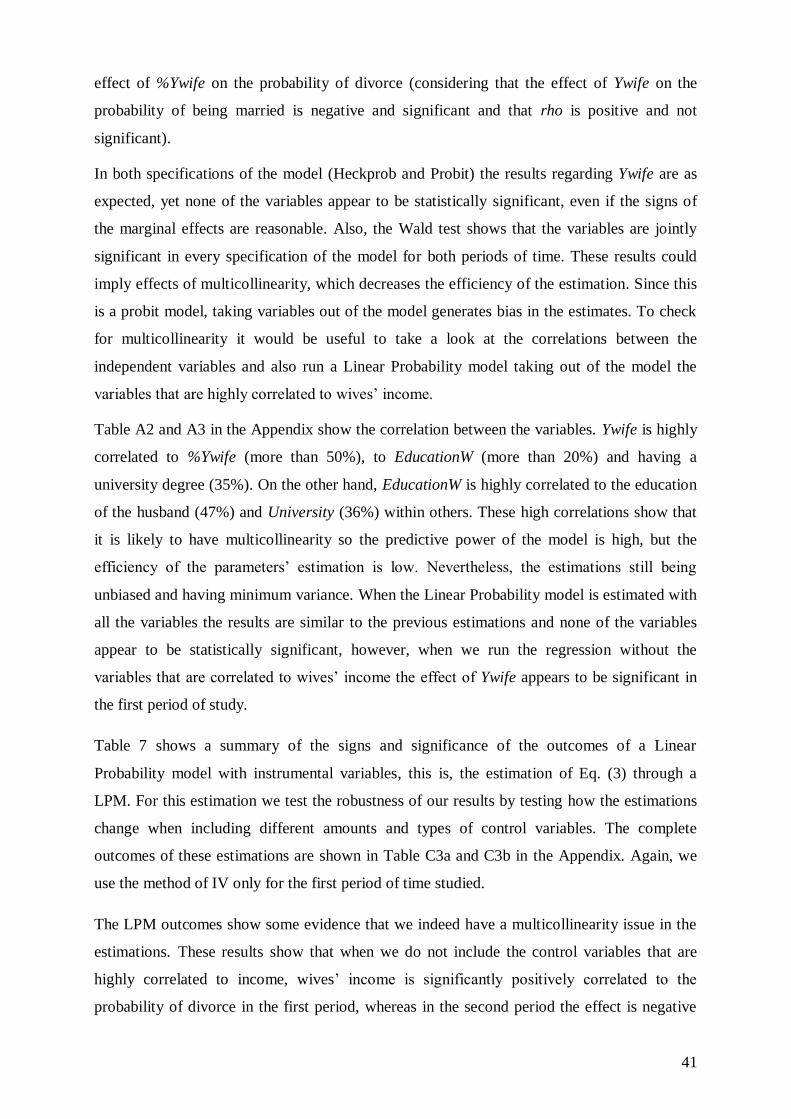
41

effect of %Ywife on the probability of divorce (considering that the effect of Ywife on the

probability of being married is negative and significant and that rho is positive and not

significant).

In both specifications of the model (Heckprob and Probit) the results regarding Ywife are as

expected, yet none of the variables appear to be statistically significant, even if the signs of

the marginal effects are reasonable. Also, the Wald test shows that the variables are jointly

significant in every specification of the model for both periods of time. These results could

imply effects of multicollinearity, which decreases the efficiency of the estimation. Since this

is a probit model, taking variables out of the model generates bias in the estimates. To check

for multicollinearity it would be useful to take a look at the correlations between the

independent variables and also run a Linear Probability model taking out of the model the

variables that are highly correlated to wives‟ income.

Table A2 and A3 in the Appendix show the correlation between the variables. Ywife is highly

correlated to %Ywife (more than 50%), to EducationW (more than 20%) and having a

university degree (35%). On the other hand, EducationW is highly correlated to the education

of the husband (47%) and University (36%) within others. These high correlations show that

it is likely to have multicollinearity so the predictive power of the model is high, but the

efficiency of the parameters‟ estimation is low. Nevertheless, the estimations still being

unbiased and having minimum variance. When the Linear Probability model is estimated with

all the variables the results are similar to the previous estimations and none of the variables

appear to be statistically significant, however, when we run the regression without the

variables that are correlated to wives‟ income the effect of Ywife appears to be significant in

the first period of study.

Table 7 shows a summary of the signs and significance of the outcomes of a Linear

Probability model with instrumental variables, this is, the estimation of Eq. (3) through a

LPM. For this estimation we test the robustness of our results by testing how the estimations

change when including different amounts and types of control variables. The complete

outcomes of these estimations are shown in Table C3a and C3b in the Appendix. Again, we

use the method of IV only for the first period of time studied.

The LPM outcomes show some evidence that we indeed have a multicollinearity issue in the

estimations. These results show that when we do not include the control variables that are

highly correlated to income, wives‟ income is significantly positively correlated to the

probability of divorce in the first period, whereas in the second period the effect is negative

42

and not significant. The Linear Probability Model shows that the effect is positive for both

measures of wives‟ income in the first period. The effect of Ywife gets reduced in the second

period, and the effect of %YWife becomes positive and signifficant.

These results show that the effect of wives‟ income on the chances of divorce in the first

period is positive robust. Nevertheless, even when we take all sources of collinearity out of

the model and we use different specifications, the effect of wives‟ income is not significantly

different from zero in the second period of time so it is possible to conclude that wives‟

income does not significantly affect the probability of divorce after the Divorce Law. Also,

the effect of %Ywife is not significant in the first period of time for every specification (even

when we take all sources of multicollinearity out of the model) so there is not enough

evidence to tell if %Ywife has an effect on the probability of divorce before the law. However

it is interesting to see that the effect of %Ywife becomes positive and significant after the

inclusion of the divorce law.

Table 7: Signs of the Effects of Wives’ Income on the Chance of Divorce using a LPM

with Instrumental Variables

Variable Without

Controls25

With all Controls

Income Wife 1996

+** +

% Income Wife 1996

+ +

Income Wife 2001

- -

% Income Wife 2001

+ +*

Even if the linear probability model is not the ideal model to regress binomial variables

because it could predict outcomes that are bigger than 1 or negative, it has the advantage that

it is possible to test for multicollinearity by taking out the correlated variables. The complete

outcomes of the LPM regressions are shown in tables C3a and C3b of the Appendix.

The estimated effects of each of the control variables are as expected and robust. In every

specification of the model and in every year the number of children and the age of the wife

25 The different specifications of the LPM, using different amount of control variables are in tables C3a and C3b

of the Appendix.

43

affect negatively the probability of divorce. On the other hand, living in an urban area,

education of both wife and husband and economic hardship increase the odds of divorce.

These could be further reasons to think that the variable of interest, i.e. wives‟ economic

situation, does affect the odds of divorce in the first period (before the Divorce Law) even if

the effect appears not to be statistically different from zero.

To test for the hypothesis that the divorce law creates two different behavioural models, one

for poor families and another for the rest of the population, I estimate Eq. (4), a LPM that

instead of only having Ywife as explanatory variable it adds an interaction variable,

Dhy*Ywife. Dhy is a dummy variable that is 1 if the family has an income higher than

$500.000 (1000 USD) and zero otherwise. When including Dhy*Ywife in the model, I can see

if there are two different behavioural models in the sample. Table 8 shows a summary of the

results of the LPM with the interaction variables and the outcome of the complete regression

is shown in table C4a and C4b in the Appendix. As expected, there is a significantly different

effect of the divorce law for poor families because the economic compensation does not fully

apply for them.

Variable Total Household Income

Difference <$500.000 >$500.000

Income Wife 1996

1.55E-07 1.44E-07 -1.14E-08

Income Wife 2001

1.80e-07 -4.50E-08 -2.25e-07*

Effect of Wives’ Income on the Odds of Divorce after the introduction of the divorce law

The analysis of the effect of wives‟ income on the probability of divorce after the introduction

of the divorce law is relatively straightforward. The relationship appears to be positive in the

first period of time and then decrease in the second period only if the family is relatively rich.

If we see the effect that this law has on families with an income over $500.000 (around 1000

USD) the effect decreases substantially in the second period of time (when the new regulation

is inserted). Interestingly, the law has no effect for families with less than $500.000 a month.

The divorce law makes the effect of wives‟ income on the odds of divorce significantly lower

for families with more than $500.000 but it has no effect on the rest of the population, where

the effect keeps being positive and even bigger than in the first period.

Table 8: Sign of the Effect of Wives’ income in the Odds

of Divorce for different Income Segments

44

The next graphs illustrate the different effects that the Divorce Law has on the coefficient of

Ywife in higher and lower income families. The graphs reflect the regression‟s outcomes when

dividing the sample between families with more than $500.000 and less than that amount of

money as total household income.

45

Graph 1: Linear Regression Line of Wives’ Income and the Predicted Probability of

Divorce for the whole sample.

1996-2001 2001-2006

Graph 2: Linear Regression Line of Wives’ Income and the Predicted Probability of

Divorce for families with a Total Income >$300.000.

1996-2001 2001-2006

Graph 3: Linear Regression Line of Wives’ Income and the Predicted Probability of

Divorce for families with a Total Income <$300.000.

1996-2001 2001-2006

As an extra exercise, I also tested if there was a significant difference in the coefficient of

%Ywife between rich and poor families but the results were not as decisive as for the case of

Ywife; moreover, the difference turned out to be negative but not significant so the results are

not reported. In general, and opposing to what was found about the effect of wives‟ income on

the probability of divorce, there is not enough evidence to state if there is an effect of %Ywife

on the probability of divorce or before the divorce law, however in the second period the

effect is positive.

The fact that the results regarding %Ywife are not as conclusive as the findings regarding

Ywife could point out that the behavioural model behind the Independence Hypothesis in

Chile before 2004 (Divorce Law) was more closely related to the Household Bargaining

theory than to Becker‟s theory (Unitary models). This, because it is an increase in the outside

option (threat point) and not a change in the ratio of utility inside and outside marriage, what

makes the probability of divorce increase. However, the inclusion of the law makes the effect

of %Ywife increase, showing evidence of a shift in the model. The insertion of the divorce law

makes more important the ratio between a wife‟s income and her household‟s total income

more important when deciding to get divorce than her earnings as such.

The effects of the divorce law for the whole population are summarized in table 9. As

expected, the results show that the effects of education and age increase with the insertion of

the Divorce Law and the effect of wives‟ income decreases; nevertheless, as stated before,

there is not enough evidence to tell if %Ywife has any effect on the probability of divorce in

the first period.

Overall, the results of this investigation support the Independence Hypothesis when

measuring wives‟ economic independence through their income, and the expected effect of

the divorce law is in line with the hypothesis also.

Method Variable Marginal

Effect 1996 Marginal

Effect 2001 Change

Heckprob

Income Wife 9.40E-07 -1.59e-06 Negative

% Income Wife

-0.233 0.356 Positive

Education 0.0178 0.0312* Positive

Age -0.0188** -0.00885 Positive

Probit

Income Wife 1.34E-07 -1.65e-06 Negative

% Income Wife

0.349 0.480* Positive

Education 0.0121 0.0302* Positive

Age -0.0194*** -0.0101** Negative

LPM

Income Wife 2.08E-08 -7.03e-08 Negative

% Income Wife

0.0157 0.0326* Positive

Education 0.00175 0.00186* Positive

Age -0.000895*** -0.000603** Positive

Table 9: Summary of the Marginal Effects and Changes for

the different specifications of the Model

7 Conclusion

The hypothesis of this investigation is that an increase in wives‟ income will increase the odds

of marital disruption in Chile. The main argument behind this hypothesis is that economic

independence will provide women with the necessary means to leave an unhappy marriage

whereas wives that depend economically on their husband will not. Besides opening the way

out of marriage, an increase in wives‟ economic assets could enhance the perception of

unfairness in the division of labour within the family and deteriorate the marital satisfaction.

The Independence Hypothesis explained above is based on traditional gender specialization,

which means that couples that are used to separate the roles of provision and housework,

loose the marital equilibrium when the one in charge of the housework decides to provide

income as well.

Chile is a country that is relatively close to the idea of traditional gender specialization while

at the same time it is rapidly developing towards gender-egalitarian ideas such as women

joining the working force. These factors make Chile an interesting society to test the

Independence Hypothesis. The actual married generation grew up in families where the

husband worked and the wife did the housework, nevertheless those daughters where

educated in the same way that their brothers. This generation still has a conservative view of

the gender roles; nevertheless, in general, both spouses provide income to the household. The

Independence Hypothesis proposes that these cases are more likely to end up separated unless

the housework role is also shared.

An example of the social development of Chile is the introduction of a law that legally allows

married couples to divorce. This law has come into effect in 2004 and has set a whole new

legal guideline that regulates the divorce procedure. One of the regulations in that law is that

the working spouse has to compensate the other one if he or she ceased, totally or partially, to

work in order to take care of the house or the family. That compensation depends on the hours

of work that the non-working spouse gave up, on their level of education, years married, and

economic situation of the working spouse. The economic compensation should only have an

effect if the wives‟ husbands can afford it. This compensation should have a negative effect

on the income-divorce relation, a result that was tested by comparing the marginal effect of

wives‟ income on the probability of divorce before and after the introduction of the law.

The results show a positive correlation between wives‟ income and divorce, effect that gets

reduced considerably with the divorce law, even becoming negative. The effect of wives‟

49

income on the risk of divorce decreases substantially in the second period for families with a

total household income larger than $500.000, showing no change for the rest of the Chilean

society. These results show that the divorce law does have an effect on the correlation

between wives‟ economic resources and the probability of divorce, but only in relatively

wealthy families because those are the ones that can afford the economic compensation in

case of marital disruption.

In conclusion, this investigation finds empirical support for both of the hypotheses. A rise in

wives‟ income increases the odds of divorce and the divorce law has an effect on that

correlation because the economic compensation protects the non-working women by

providing them with the means that are necessary to finish their marriage if they want to. This

obviously provokes that the effect of the wives‟ income on the risk of divorce is less

important with the divorce law, because the compensation works as a substitute of wives‟

income. However, since the economic compensation only matters in case the husband is able

to pay for it, only rich men‟s wives benefit from the divorce law‟s compensation scheme,

while having no effect on the poor.

The interesting finding of this study is that, due to the specifications of the divorce law, the

obligation to compensate the non-working spouse does not have an effect for everyone;

moreover, it applies only for the part of the society with higher income. This induces

differences of behaviour, when relating marital disruption and income, between rich and poor

families. The part of the society that has weakest incentives to work in case they have

undesirable marriages are the non-working but educated women that are married to rich men,

in fact, they could end up having economic gains in case of divorce. On the other hand, the

most divorce-averse wives, or in other words, the wives that have the stronger incentives to

work in case they have undesirable marriages, are the non-working spouses of poor husbands,

because if they do not work, even if they have undesirable marriages, they don‟t have the

means to leave them.

8 References

Becker, G. (1981). A Treatise on the Family. Harvard University Press.

Bedard, K. and Deschenes, O. (2003). Sex Preferences, Marital Dissolution, and the

Economic Status of Women. Departmental Working Papers, Department of Economics,

UCSB, UC Santa Barbara.

Bergstrom, T. (1993). Marriage Markets and Bargaining Between Spouses. Journal of

Political Economy.

Binmore, K., Rubinstein, A. and Wolinsky, A. (1986). The Nash Bargaining Solution in

Economic Modelling. Rand Journal of Economics. Vol.17, No.2.

Blumberg R. L., & Coleman, M. T. (1989). A Theoretical Look at the Gender Balance of

Power in the American Couple. Journal of Family Issues. Vol. 10, pp. 225-250.

Booth, A., Johnson, D., White, L. and Edwards, J. (1984). Women, Outside Employment, and

Marital Instability. The American Journal of Sociology. Vol. 90, No. 3, pp. 567-583.

Burges, S., Propper, C. and Aassve, A. (2003). The Role of Income in Marriage and Divorce

Transitions among Young Americans. Journal of Population Economics. Vol. 16, No. 3, pp.

455-475.

Chiappori, P.A., Iyigun, M. and Weiss, Y. (2008). An Assignment Model with Divorce and

Remarriage. IZA Discussion Paper. No. 3892. Available at SSRN:

http://ssrn.com/abstract=1318851

Coltrane, S. (1996). Family man: Fatherhood, Housework and Gender Equity. New York:

Oxford University Press.

Dubin, J. and Rivers, D. (1989). Selection bias in Linear Regression, Logit and Probit

Models. Sociological Methods and Research. Vol. 18, Nos. 2 & 3.

Greenstein, T. N. (1990). Marital Disruption and the Employment of Married Women.

Journal of Marriage and the Family. Vol. 52, 657-676.

Heckert, D. A., Nowak, T. C., & Snyder, K. A. (1998). The Impact of Husbands' and Wives'

Relative Earnings on Marital Disruption. Journal of Marriage and the Family. Vol. 60, 690-

703.

51

Heckman, J. J. (1979). Sample Selection Bias as a Specification Error. Econometrica, 47,

151–161.

Hiedemann, B., Suhomlinova, O. and O‟Rand, A. (1998). Economic Independence, Economic

Status, and Empty Nest in Midlife Marital Disruption. Journal Of Marriage and Family. Vol.

60, No. 1, pp. 219-231.

Jalovaara, M. (2003). The joint effects of marriage partners‟ socioeconomic positions on the

risk of divorce. Demography 40(1), 67–81.

Johnson, W. and Skinner, J. (1986). Labor Supply and Marital Separation. The American

Economic Review, Vol. 76, No. 3, pp. 455-469.

Kesselring, R. G. and Bremmer, D. (2006). Female Income and the Divorce Decision:

Evidence from Micro Data”. Applied Economics. Vol. 38(14), pp. 1605-1616.

Knoester, C. and Booth, A. (2000). Barriers to Divorce: When are they effective? When are

they not? Journal of Family Issues. Vol. 21, No. 1, pp. 78-99.

Kraft, K. and Neimann, S. (2009). Labor division between wife and husband and the risk of

divorce: New evidence from Germany. First Draft.

Lehmann, C. and Hinzpeter, X. (1995). Where are the Conservative Forces of the Chilean

Society? Estudios Publicos; vol. 60.

Lehmann, C. (2003). Women, Work and Family: Reality, Perceptions and Challenges:

Analysis based on the CEP Survey of December 20002. Estudios Publicos. Vol. 269.

Liu, G. and Vikat, A. (2004). Does divorce risk depend on spouses' relative income? A

register-based study of first marriages in Sweden in 1981-1998. MPIDR Working Paper WP

2004-010.

Lundberg, S and Pollak, R. (1993). Separate Spheres Bargaining and the Marriage Market.

The Journal of Political Economy. Vol. 101, No. 6, pp. 988-1010.

Manser, M. and Brown, M. (1980). Marriage and Household Decision-making: A Bargaining

Analysis. International Economic Review. Vol. 21, No. 1, pp.31-44.

Manting, D. and Bouman, A.M. (2004). Short- and Long-Term Economic Consequences of

the Dissolution of Marital and Consensual Unions. The Example of the Netherlands. Oxford

University Press. Vol. 22, No. 4, pp. 413-429.

52

McElroy, M. and Horney, M.J. (1981). Nash-bargained Household decisions: Toward a

Generalization of the Theory of Demand. International Economic Review. Vol. 22. No. 2, pp.

333-349.

Nock, S. L. (1995). Commitment and Dependency in Marriage. Journal of Marriage and the

Family. Vol. 57, pp. 503-514.

Nunley, J. (2007). The effect of Household Income Volatility on Divorce. Working Papers,

Middle Tennessee State University, Department of Economics and Finance. No. 200718.

Available at http://econpapers.repec.org/RePEc:mts:wpaper:200718.

Ono, H. (1998) Husbands' and Wives' Resources and Marital Dissolution. Journal of

Marriage and Family. Vol. 60, No. 3, pp. 674-689

Page, M. and Huff, A. (2002). “Will you miss me when I‟m Gone? The Economic

Consequences of Absent Parents”. NBER Working Paper. No. W8786. Available at SSRN:

http://ssrn.com/abstract=300748

Parsons, T. (1959). The social structure of the family. In R.N. Anshen (Ed.), The family: Its

function and destiny, Harper; pp. 241-273.

Risman, B . J., & Johnson-Sumerford, D. (1998). Doing it fairly: A study of post gender

marriages. Journal of Marriage and the Family. Vol. 60, pp. 23-40.

Rogers, S. (2004). Dollars, Dependency, and Divorce: Four Perspectives on the role of wives‟

income. Journal of Marriage and Family; vol. 66, No. 1, pp. 59-74.

Sander, W. (1985). Women, work and Divorce. The American Economic Review. Vol. 75, No.

3, pp. 519-523

Sanhueza, C., Bravo, D. and Quijada, S. (2007). An Empirical Analysis of the Socioeconomic

Determinants of Marital Dissolution in Chile. University of Chile Working Papers; vol. 250.

Sayer, L. C. and Bianchi, S. M. (2000). Women's Economic Independence and the Probability

of Divorce. Journal of Family Issues. Vol. 21(7); pp. 906-943.

Spitze, G. and South, S. J. (1985). Women's Employment, Time Expenditure, and Divorce.

Journal of Family Issues. Vol. 6(3), pp. 307-329.

Tzeng, J. M. and Mare, R. D. (1995). Labor market and Socioeconomic effects on Marital

Stability. Social Science Research. Vol. 24(4), pp. 329-351

53

Van de Ven, W. and Van Praag, B. (1981). The Demand for Deductibles in Private Health

Insurance : A Probit Model with Sample Selection. Journal of Econometrics. Vol. 17(2), pp.

229-252.

Wooldridge, Jeffrey. (2001). Econometric Analysis of Cross Section and Panel Data. The MIT

Press, Cambridge, Massachusetts.

9 Appendix

Ley De Matrimonio Civil (1884)

Capítulo III.

1. De la separación de hecho

Artículo 21.- Si los cónyuges se separaren de hecho, podrán, de común acuerdo, regular sus

relaciones mutuas, especialmente los alimentos que se deban y las materias vinculadas al

régimen de bienes del matrimonio. En todo caso, si hubiere hijos, dicho acuerdo deberá

regular también, a lo menos, el régimen aplicable a los alimentos, al cuidado personal y a la

relación directa y regular que mantendrá con los hijos aquél de los padres que no los tuviere

bajo su cuidado. Los acuerdos antes mencionados deberán respetar los derechos conferidos

por las leyes que tengan el carácter de irrenunciables.

Artículo 22.- El acuerdo que conste por escrito en alguno de los siguientes instrumentos

otorgará fecha cierta al cese de la convivencia:

a) escritura pública, o acta extendida y protocolizada ante notario público;

b) acta extendida ante un Oficial del Registro Civil, o

c) transacción aprobada judicialmente.

No obstante lo dispuesto en el inciso anterior, si el cumplimiento del acuerdo requiriese una

inscripción, subinscripción o anotación en un registro público, se tendrá por fecha del cese de

la convivencia aquélla en que se cumpla tal formalidad. La declaración de nulidad de una o

más de las cláusulas de un acuerdo que conste por medio de alguno de los instrumentos

señalados en el inciso primero, no afectará el mérito de aquél para otorgar una fecha cierta al

cese de la convivencia.

Artículo 23.- A falta de acuerdo, cualquiera de los cónyuges podrá solicitar que el

procedimiento judicial que se sustancie para reglar las relaciones mutuas, como los alimentos

que se deban, los bienes familiares o las materias vinculadas al régimen de bienes del

matrimonio; o las relaciones con los hijos, como los alimentos, el cuidado personal o la

relación directa y regular que mantendrá con ellos el padre o madre que no los tuviere bajo su

cuidado, se extienda a otras materias concernientes a sus relaciones mutuas o a sus relaciones

con los hijos.

Artículo 24.- Las materias de conocimiento conjunto a que se refiere el artículo precedente se

ajustarán al mismo procedimiento establecido para el juicio en el cual se susciten. En la

resolución que reciba la causa a prueba, el juez fijará separadamente los puntos que se

refieran a cada una de las materias sometidas a su conocimiento. La sentencia deberá

pronunciarse sobre todas las cuestiones debatidas en el proceso.

Artículo 25.- El cese de la convivencia tendrá también fecha cierta a partir de la notificación

de la demanda, en el caso del artículo 23. Asimismo, habrá fecha cierta, si no mediare acuerdo

ni demanda entre los cónyuges, cuando, habiendo uno de ellos expresado su voluntad de

poner fin a la convivencia a través de cualquiera de los instrumentos señalados en las letras a)

y b) del artículo 22 o dejado constancia de dicha intención ante el juzgado correspondiente, se

notifique al otro cónyuge. En tales casos, se tratará de una gestión voluntaria y se podrá

comparecer personalmente. La notificación se practicará según las reglas generales.

2. De la separación judicial

55

1. De las causales.

Artículo 26.- La separación judicial podrá ser demandada por uno de los cónyuges si mediare

falta imputable al otro, siempre que constituya una violación grave de los deberes y

obligaciones que les impone el matrimonio, o de los deberes y obligaciones para con los hijos,

que torne intolerable la vida en común. No podrá invocarse el adulterio cuando exista previa

separación de hecho consentida por ambos cónyuges. En los casos a que se refiere este

artículo, la acción para pedir la separación corresponde únicamente al cónyuge que no haya

dado lugar a la causal.

Artículo 27.- Sin perjuicio de lo anterior, cualquiera de los cónyuges podrá solicitar al tribunal

que declare la separación, cuando hubiere cesado la convivencia. Si la solicitud fuere

conjunta, los cónyuges deberán acompañar un acuerdo que regule en forma completa y

suficiente sus relaciones mutuas y con respecto a sus hijos. El acuerdo será completo si regula

todas y cada una de las materias indicadas en el artículo 21. Se entenderá que es suficiente si

resguarda el interés superior de los hijos, procura aminorar el menoscabo económico que

pudo causar la ruptura y establece relaciones equitativas, hacia el futuro, entre los cónyuges

cuya separación se solicita.".

2. Del ejercicio de la acción.

Artículo 28.- La acción de separación es irrenunciable.

Artículo 29.- La separación podrá solicitarse también en el procedimiento a que dé lugar

alguna de las acciones a que se refiere el artículo 23, o una denuncia por violencia

intrafamiliar producida entre los cónyuges o entre alguno de éstos y los hijos.

Artículo 30.- Tratándose de cónyuges casados bajo el régimen de sociedad conyugal,

cualquiera de ellos podrá solicitar al tribunal la adopción de las medidas provisorias que

estime conducentes para la protección del patrimonio familiar y el bienestar de cada uno de

los miembros que la integran. Lo dispuesto en el presente artículo se aplicará sin perjuicio del

derecho que asiste a las partes de solicitar alimentos o la declaración de bienes familiares,

conforme a las reglas generales.

Artículo 31.- Al declarar la separación, el juez deberá resolver todas y cada una de las

materias que se señalan en el artículo 21, a menos que ya se encontraren reguladas o no

procediere la regulación judicial de alguna de ellas, lo que indicará expresamente. Tendrá en

especial consideración los criterios de suficiencia señalados en el artículo 27.

El juez utilizará los mismos criterios al evaluar el acuerdo presentado o alcanzado por los

cónyuges, procediendo en la sentencia a subsanar sus deficiencias o modificarlo si fuere

incompleto o insuficiente. En la sentencia el juez, además, liquidará el régimen matrimonial

que hubiere existido entre los cónyuges, si así se le hubiere solicitado y se hubiere rendido la

prueba necesaria para tal efecto.

3. De los efectos

Artículo 32.- La separación judicial produce sus efectos desde la fecha en que queda

ejecutoriada la sentencia que la decreta. Sin perjuicio de ello, la sentencia ejecutoriada en que

se declare la separación judicial deberá subinscribirse al margen de la respectiva inscripción

matrimonial. Efectuada la subinscripción, la sentencia será oponible a terceros y los cónyuges

adquirirán la calidad de separados, que no los habilita para volver a contraer matrimonio.

Artículo 33.- La separación judicial deja subsistentes todos los derechos y obligaciones

personales que existen entre los cónyuges, con excepción de aquellos cuyo ejercicio sea

incompatible con la vida separada de ambos, tales como los deberes de cohabitación y de

56

fidelidad, que se suspenden.

Artículo 34.- Por la separación judicial termina la sociedad conyugal o el régimen de

participación en los gananciales que hubiere existido entre los cónyuges, sin perjuicio de lo

dispuesto en el artículo 147 del Código Civil.

Artículo 35.- El derecho de los cónyuges a sucederse entre sí no se altera por la separación

judicial. Se exceptúa el caso de aquél que hubiere dado lugar a la separación por su culpa, en

relación con el cual el juez efectuará en la sentencia la declaración correspondiente, de la que

se dejará constancia en la subinscripción.

Tratándose del derecho de alimentos, regirán las reglas especiales contempladas en el Párrafo

V, del Título VI del Libro Primero del Código Civil.

Artículo 36.- No se alterará la filiación ya determinada ni los deberes y responsabilidades de

los padres separados en relación con sus hijos. El juez adoptará todas las medidas que

contribuyan a reducir los efectos negativos que pudiera representar para los hijos la

separación de sus padres.

Artículo 37.- El hijo concebido una vez declarada la separación judicial de los cónyuges no

goza de la presunción de paternidad establecida en el artículo 184 del Código Civil. Con todo,

el nacido podrá ser inscrito como hijo de los cónyuges, si concurre el consentimiento de

ambos.

…

Artículo 107. Los que no hubieren cumplido dieciocho años no podrán casarse sin el

consentimiento expreso de sus padres; si faltare uno de ellos, el del otro padre o madre; o a

falta de ambos, el del ascendiente o de los ascendientes de grado más próximo. En igualdad

de votos contrarios preferirá el favorable al matrimonio. (Ley 19585, Art. 1º Nº 13)

Nueva Ley de Matrimonio Civil (Mayo, 2004)

Párrafo 3º (Capítulo VI)

De los efectos

Artículo 59.- El divorcio producirá efectos entre los cónyuges desde que quede ejecutoriada la

sentencia que lo declare. Sin perjuicio de ello, la sentencia ejecutoriada en que se declare el

divorcio deberá subinscribirse al margen de la respectiva inscripción matrimonial. Efectuada

la subinscripción, la sentencia será oponible a terceros y los cónyuges adquirirán el estado

civil de divorciados, con lo que podrán volver a contraer matrimonio.

Artículo 60.- El divorcio pone fin a las obligaciones y derechos de carácter patrimonial cuya

titularidad y ejercicio se funda en la existencia del matrimonio, como los derechos sucesorios

recíprocos y el derecho de alimentos, sin perjuicio de lo dispuesto en el Párrafo 1 del Capítulo

siguiente.

Capítulo VII

De las reglas comunes a ciertos casos de separación, nulidad y divorcio

Párrafo 1º

De la compensación económica

Artículo 61.- Si, como consecuencia de haberse dedicado al cuidado de los hijos o a las

labores propias del hogar común, uno de los cónyuges no pudo desarrollar una actividad

57

remunerada o lucrativa durante el matrimonio, o lo hizo en menor medida de lo que podía y

quería, tendrá derecho a que, cuando se produzca el divorcio o se declare la nulidad del

matrimonio, se le compense el menoscabo económico sufrido por esta causa.

Artículo 62.- Para determinar la existencia del menoscabo económico y la cuantía de la

compensación, se considerará, especialmente, la duración del matrimonio y de la vida en

común de los cónyuges; la situación patrimonial de ambos; la buena o mala fe; la edad y el

estado de salud del cónyuge beneficiario; su situación en materia de beneficios previsionales

y de salud; su cualificación profesional y posibilidades de acceso al mercado laboral, y la

colaboración que hubiere prestado a las actividades lucrativas del otro cónyuge. Si se

decretare el divorcio en virtud del artículo 54, el juez podrá denegar la compensación

económica que habría correspondido al cónyuge que dio lugar a la causal, o disminuir

prudencialmente su monto.

Artículo 63.- La compensación económica y su monto y forma de pago, en su caso, serán

convenidos por los cónyuges, si fueren mayores de edad, mediante acuerdo que constará en

escritura pública o acta de avenimiento, las cuales se someterán a la aprobación del tribunal.

Artículo 64.- A falta de acuerdo, corresponderá al juez determinar la procedencia de la

compensación económica y fijar su monto. Si no se solicitare en la demanda, el juez

informará a los cónyuges la existencia de este derecho durante la audiencia preparatoria.

Pedida en la demanda, en escrito complementario de la demanda o en la reconvención, el juez

se pronunciará sobre la procedencia de la compensación económica y su monto, en el evento

de dar lugar a ella, en la sentencia de divorcio o nulidad.

Artículo 65.- En la sentencia, además, el juez determinará la forma de pago de la

compensación, para lo cual podrá establecer las siguientes modalidades:

1.- Entrega de una suma de dinero, acciones u otros bienes. Tratándose de dinero, podrá ser

enterado en una o varias cuotas reajustables, respecto de las cuales el juez fijará seguridades

para su pago.

2.- Constitución de derechos de usufructo, uso o habitación, respecto de bienes que sean de

propiedad del cónyuge deudor. La constitución de estos derechos no perjudicará a los

acreedores que el cónyuge propietario hubiere tenido a la fecha de su constitución, ni

aprovechará a los acreedores que el cónyuge beneficiario tuviere en cualquier tiempo.

Artículo 66.- Si el deudor no tuviere bienes suficientes para solucionar el monto de la

compensación mediante las modalidades a que se refiere el artículo anterior, el juez podrá

dividirlo en cuantas cuotas fuere necesario. Para ello, tomará en consideración la capacidad

económica del cónyuge deudor y expresará el valor de cada cuota en alguna unidad

reajustable. La cuota respectiva se considerará alimentos para el efecto de su cumplimiento, a

menos que se hubieren ofrecido otras garantías para su efectivo y oportuno pago, lo que se

declarará en la sentencia.

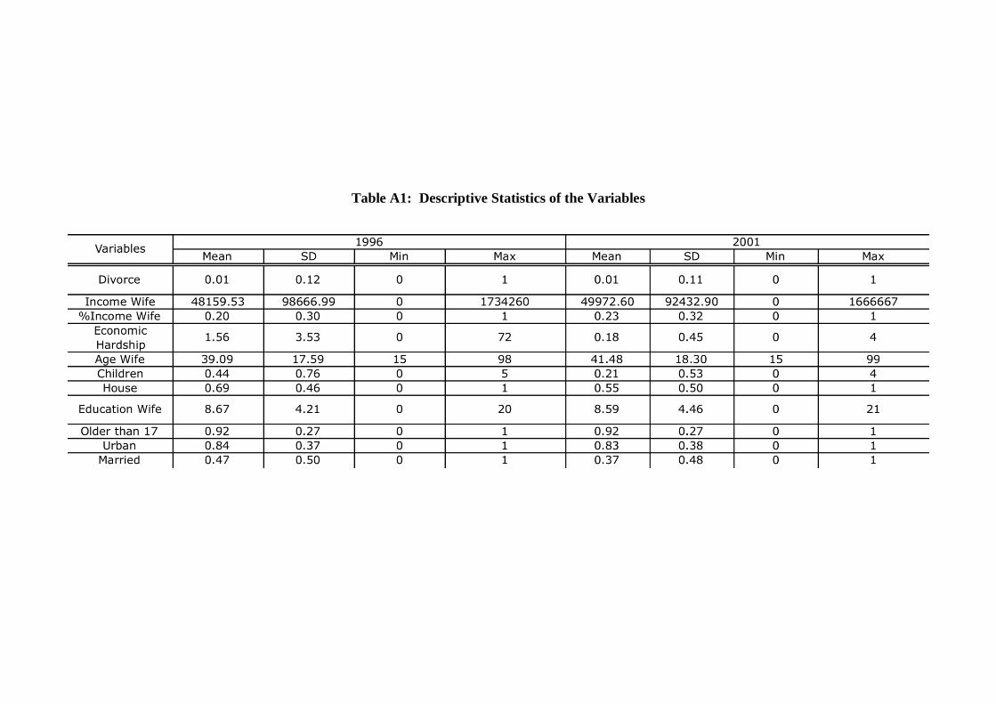
Table A1: Descriptive Statistics of the Variables

Table A2: Correlations Matrix for all the Variables in the model of period 1996

Table A3: Correlations Matrix for all the Variables in the model of period 2001

60

Table B1a (1996): First Stage OLS Estimation for Wives’ Income in 1996

VARIABLES OLS

Estimations

Boss 277,291*** (14,702)

Independent 67,930***

(4,978)

Public Employee 153,262*** (5,815)

Private Employee 126,615***

(3,662) Armed Force 100,450**

(40,603)

Family Work -15,647 (14,207)

Domestic Employee 58,634***

(5,345)

3rd Region -9,872* (5,303)

7th Region -1,017

(3,331) Metrop. Region 11,879***

(2,741)

HParent University Degree 54,662*** (15,509)

HParent Technical Degree -5,941

(28,767)

HParent Highschool Degree -15,838*** (4,726)

Children 1,656

(1,627) Urban -2,852

(3,124)

AgeW 1,496***

(77.57) EducationW 4,096***

(352.1)

Economic Hardship -782.3** (308.5)

Owns House -8,641***

(2,540) EducationH 677.8***

(230.4)

Constant -74,643***

(5,693)

Observations 5,084

R-squared 0.408

Standard errors in parentheses

*** p<0.01, ** p<0.05, * p<0.1

61

Table B1a (2001): First Stage OLS Estimation for Wives’ Income in 2001

VARIABLES OLS

Estimations

Boss 197,809***

(10,655)

Independent 77,486***

(4,469)

Public Employee 150,767***

(4,907)

Private Employee 105,921***

(3,162)

Armed Force 101,446

(75,260)

Family Work -12,508

(11,812)

Domestic Employee 61,610***

(5,392)

3rd Region -7,583

(4,702)

7th Region -6,856**

(3,054)

Metrop. Region -607.2

(2,437)

HParent University Degree 37,834***

(11,428)

HParent Technical Degree 1,536

(20,918) HParent Highschool Degree -22,286***

(2,433)

Children -107.0

(1,852)

Urban 3,165

(2,940)

AgeW 1,953***

(77.32)

EducationW 4,680***

(332.9)

Economic Hardship -5,517***

(2,044)

Owns House -13,153***

(2,518)

EducationH 297.9

(202.7)

Constant -89,322***

(6,058)

Observations 5,309

R-squared 0.400

Standard errors in parentheses

*** p<0.01, ** p<0.05, * p<0.1

62

Table B1b (1996): First Stage OLS Estimation for Wives’ Income as a Percentage of Total Household

Income in 1996

VARIABLES OLS

Estimations

3rd Region -0.0322**

(0.0154)

7th Region -0.0234** (0.00968)

Metrop. Region -0.0161**

(0.00799) HParent University Degree 0.0385

(0.0458)

HParent Technical Degree 0.0865

(0.0834) HParent Highschool Degree -0.00779

(0.0138)

Boss 0.338*** (0.0426)

Independent 0.269***

(0.0144) Public Employee 0.418***

(0.0169)

Private Employee 0.380***

(0.0106) Armed Force 0.570***

(0.118)

Family Work -0.0324 (0.0412)

Domestic Employee 0.317***

(0.0155) Children -0.00870*

(0.00474)

Urban 0.0440***

(0.00908) AgeW 0.00639***

(0.000226)

EducationW 0.00257** (0.00103)

Economic Hardship -0.00316***

(0.000898)

Owns House -0.0967*** (0.00741)

EducationH -0.00829***

(0.000673) Constant -0.0390**

(0.0166)

Observations 5,248

R-squared 0.413

Standard errors in parentheses

*** p<0.01, ** p<0.05, * p<0.1

63

Table B1b (2001): First Stage OLS Estimation for Wives’ Income as a Percentage of Total Household

Income in 2001

VARIABLES OLS

Estimations

3rd Region -0.0244

(0.0158)

7th Region -0.0336*** (0.0103)

Metrop. Region -0.0160*

(0.00822) HParent University Degree 0.0340

(0.0387)

HParent Technical Degree 0.0722

(0.0701) HParent Highschool Degree -0.0138*

(0.00820)

Boss 0.360*** (0.0357)

Independent 0.303***

(0.0150) Public Employee 0.421***

(0.0165)

Private Employee 0.390***

(0.0106) Armed Force 0.916***

(0.252)

Family Work -0.116*** (0.0396)

Domestic Employee 0.311***

(0.0181) Children -0.00942

(0.00625)

Urban 0.0489***

(0.00990) AgeW 0.00753***

(0.000260)

EducationW 0.00293*** (0.00113)

Economic Hardship 0.00696

(0.00687)

Owns House -0.148*** (0.00849)

EducationH -0.00798***

(0.000691) Constant -0.0440**

(0.0205)

Observations 5,248

R-squared 0.407

Standard errors in parentheses

*** p<0.01, ** p<0.05, * p<0.1

64

Table C1a: Marginal Effects Probit with Heckman’s Correction with (and without) Instrumented Variables for the period between 1996-2001

VARIABLES

Marginal Effects HeckProb no Instrumented Variables

Marginal Effects HeckProb with both Instrumented Variables

Marginal Effects HeckProb with Ywife as Instrumented Variable

Marginal Effects HeckProb with %Ywife as Instrumented Variable

Divorce Marriage Athrho Divorce Marriage Athrho Divorce Marriage Athrho Divorce Marriage Athrho

%Ywife -0.409 -1.851*** -0.233 -1.866*** -0.934* -1.866*** 0.0710 -1.866*** (0.445) (0.0738) (0.817) (0.0827) (0.517) (0.0827) (0.542) (0.0827) Ywife 2.40e-07 6.06e-07*** 9.40e-07 8.28e-07*** 2.53e-06** 8.28e-07*** -7.19e-08 8.28e-07*** (5.84e-07) (2.07e-07) (1.99e-06) (2.24e-07) (1.23e-06) (2.24e-07) (7.11e-07) (2.24e-07) Residual Ywife -1.07e-06 -2.71e-06** (2.04e-06) (1.27e-06) Residual %Ywife -0.979 -1.307** (0.820) (0.551) Children -0.0811 0.413*** -0.0272 0.388*** -0.0457 0.388*** -0.0213 0.388***

(0.0951) (0.0226) (0.105) (0.0248) (0.106) (0.0248) (0.104) (0.0248) Urban 0.200 -0.0498 0.175 -0.110** 0.225 -0.110** 0.159 -0.110** (0.149) (0.0448) (0.174) (0.0473) (0.170) (0.0473) (0.170) (0.0473) AgeW -0.0144** 0.0185*** -0.0188** 0.0146*** -0.0154** 0.0146*** -0.0193** 0.0146*** (0.00627) (0.00119) (0.00784) (0.00130) (0.00718) (0.00130) (0.00781) (0.00130) EducationW 0.0203 0.0108** 0.0178 -0.0438*** 0.0148 -0.0438*** 0.0213 -0.0438*** (0.0172) (0.00503) (0.0220) (0.00552) (0.0214) (0.00552) (0.0210) (0.00552) Ecnomic Hardship 0.00677 0.0111 0.0100 0.0108

(0.0113) (0.0127) (0.0126) (0.0127) Owns House 0.0462 0.127 0.0467 0.151 (0.102) (0.138) (0.121) (0.131) University Degree -0.0563 0.425*** -0.163 1.143*** -0.183 1.143*** -0.132 1.143*** (0.265) (0.101) (0.336) (0.105) (0.340) (0.105) (0.331) (0.105) Technical Degree 0.109 -0.0287 -0.00194 0.563*** 0.00334 0.563*** 0.0133 0.563*** (0.247) (0.104) (0.274) (0.106) (0.275) (0.106) (0.273) (0.106) EducationH 0.000616 0.00558 -0.00283 0.00871

(0.0107) (0.0148) (0.0129) (0.0132) Older than 17 2.099*** 1.971*** 1.971*** 1.970*** (0.139) (0.154) (0.154) (0.154) Constant -1.809*** -2.733*** 0.198 -1.934*** -2.225*** 0.358 -1.847*** -2.225*** 0.341 -1.999*** -2.225*** 0.367 (0.452) (0.150) (0.344) (0.433) (0.165) (0.374) (0.429) (0.165) (0.374) (0.410) (0.165) (0.376) Observations 7,373 7,373 7,373 6,296 6,296 6,296 6,296 6,296 6,296 6,296 6,296 6,296

Standard errors in parentheses

*** p<0.01, ** p<0.05, * p<0.1

65

Table C1b: Marginal Effects Probit with Heckman’s Correction with (and without) Instrumented Variables for the period between 2001-2006

VARIABLES

Marginal Effects HeckProb no Instrumented Variables

Marginal Effects HeckProb with both Instrumented Variables

Marginal Effects HeckProb with Ywife as Instrumented Variable

Marginal Effects HeckProb with %Ywife as Instrumented Variable

Divorce Marriage Athrho Divorce Marriage Athrho Divorce Marriage Athrho Divorce Marriage Athrho

%Ywife 0.356 -1.661*** 0.280 -1.661*** 0.320 -1.661*** 0.319 -1.661*** (0.444) (0.0761) (0.548) (0.0761) (0.446) (0.0761) (0.548) (0.0761) Ywife -1.59e-06 3.20e-07 -1.49e-06 3.20e-07 -1.55e-06 3.20e-07 -1.53e-06 3.20e-07 (1.10e-06) (2.63e-07) (1.18e-06) (2.63e-07) (1.09e-06) (2.63e-07) (1.19e-06) (2.63e-07) Residual Ywife 7.25e-09 7.23e-09 (6.31e-09) (6.31e-09)

Residual %Ywife 0.0586 0.0533 (0.461) (0.460) Children -0.0163 0.482*** -0.0159 0.482*** -0.0132 0.482*** -0.0188 0.482*** (0.115) (0.0356) (0.117) (0.0356) (0.115) (0.0356) (0.117) (0.0356) Urban 0.142 -0.0495 0.144 -0.0494 0.141 -0.0494 0.145 -0.0495 (0.148) (0.0511) (0.150) (0.0511) (0.148) (0.0511) (0.150) (0.0511) AgeW -0.00885 0.0126*** -0.00854 0.0126*** -0.00878 0.0126*** -0.00863 0.0126*** (0.00614) (0.00150) (0.00642) (0.00150) (0.00614) (0.00150) (0.00642) (0.00150)

EducationW 0.0312* 0.0108* 0.0314* 0.0108* 0.0311* 0.0108* 0.0314* 0.0108* (0.0176) (0.00576) (0.0177) (0.00576) (0.0176) (0.00576) (0.0177) (0.00576) Ecnomic Hardship 0.236*** 0.240*** 0.239*** 0.237*** (0.0817) (0.0822) (0.0818) (0.0821) Owns House 0.0470 0.0425 0.0502 0.0400 (0.125) (0.140) (0.126) (0.139) University Degree 0.0610 0.134 0.0706 0.134 0.0724 0.134 0.0591 0.134 (0.324) (0.115) (0.323) (0.115) (0.323) (0.115) (0.324) (0.115) Technical Degree -0.263 -0.0856 -0.251 -0.0856 -0.252 -0.0856 -0.263 -0.0855

(0.324) (0.109) (0.324) (0.109) (0.324) (0.109) (0.324) (0.109) EducationH -0.00804 -0.00925 -0.00883 -0.00843 (0.0110) (0.0116) (0.0111) (0.0115) Older than 17 1.267*** 1.267*** 1.267*** 1.267*** (0.0931) (0.0931) (0.0931) (0.0931) Constant -1.967*** -1.497*** 0.112 -1.958*** -1.497*** 0.107 -1.964*** -1.497*** 0.110 -1.962*** -1.497*** 0.109 (0.470) (0.122) (0.343) (0.473) (0.122) (0.344) (0.471) (0.122) (0.344) (0.472) (0.122) (0.343)

Observations 5,248 5,248 5,248 5,248 5,248 5,248 5,248 5,248 5,248 5,248 5,248 5,248

Standard errors in parentheses

*** p<0.01, ** p<0.05, * p<0.1

Table C2a: Marginal Effects Probit with Instrumented Variables for the period

between 1996-2001

VARIABLES

Marginal Effects

PROBIT with Ywife as Instrumented Variable

Marginal Effects

PROBIT with %Ywife as Instrumented Variable

Marginal Effects

PROBIT with Ywife and %Ywife as Instrumented Variables

Divorce Ywife Divorce %Ywife Divorce %Ywife Ywife

Ywife 3.67e-06** -1.25e-06 5.40e-07*** 1.34e-07 (1.57e-06) (8.03e-07) (6.66e-08) (2.12e-06) %Ywife -1.135** 147,120*** 0.798* 0.349 (0.514) (15,403) (0.413) (0.751) Children -0.114* -494.7 -0.119** 0.00706*** -0.118* 0.00736*** 554.6

(0.0595) (1,717) (0.0594) (0.00266) (0.0601) (0.00276) (1,787) Urban 0.203 -1,953 0.203 0.00234 0.207 0.00136 -1,798 (0.145) (2,013) (0.147) (0.00645) (0.148) (0.00677) (2,135) AgeW -0.0177*** 368.2*** -0.0191*** 0.00183*** -0.0194*** 0.00221*** 693.6*** (0.00438) (104.9) (0.00449) (0.000221) (0.00460) (0.000236) (104.2) EducationW 0.00486 2,500*** 0.0158 -0.000433 0.0121 0.00103 2,688*** (0.0195) (590.0) (0.0190) (0.00107) (0.0193) (0.00109) (607.3) Economic

Hardship

0.00683 -25.19 0.00646 -0.000529 0.00655 -0.000592 -112.8

(0.00967) (190.7) (0.00992) (0.000555) (0.0100) (0.000588) (205.6) Owns House 0.0335 259.7 0.0563 -0.0155*** 0.0521 -0.0167*** -2,202 (0.103) (2,761) (0.103) (0.00523) (0.104) (0.00542) (2,888) University Degree

-0.397 81,985*** -0.0985 -0.0195 -0.206 0.0273 86,481***

(0.315) (18,213) (0.283) (0.0185) (0.346) (0.0188) (19,007) Technical

Degree

0.0245 21,859 0.152 -0.0372** 0.115 -0.0274* 18,035

(0.283) (16,325) (0.271) (0.0156) (0.290) (0.0150) (16,617) EducationH -0.00518 946.8*** 0.00442 -0.00366*** 0.00203 -0.00342*** 444.7* (0.00984) (261.0) (0.00956) (0.000500) (0.0104) (0.000527) (269.9) High School 0.0527 -9,389*** 0.0177 0.00571 0.0296 0.000635 -9,369*** (0.110) (3,456) (0.111) (0.00584) (0.112) (0.00599) (3,555) Boss 246,607*** 0.157*** 0.317*** 296,882*** (48,503) (0.0299) (0.0303) (50,521)

Independent Employee

52,329*** 0.239*** 0.291*** 95,710***

(7,494) (0.0133) (0.0127) (7,762) Public Employee

67,663*** 0.360*** 0.430*** 129,390***

(13,173) (0.0195) (0.0174) (11,926) Private employee

78,238*** 0.298*** 0.369*** 131,726***

(7,785) (0.0148) (0.0117) (7,360) Armed Force 77,288*** 0.238*** 0.305*** 123,602*** (24,898) (0.0505) (0.0636) (32,561) Domestic Employee

13,773** 0.299*** 0.334*** 63,321***

(6,133) (0.0196) (0.0198) (3,510) 3rd Region -1,107 -0.00590 -0.00753 -2,658 (4,484) (0.00937) (0.0101) (4,854) 7th Region 2,820 -0.00981 -0.00931 1,211

(2,700) (0.00637) (0.00672) (2,857) Metrop. Region 8,260*** -0.0146*** -0.0114** 6,360** (2,665) (0.00529) (0.00559) (2,788) HParent University

5,209 0.0316 0.0315 4,085

(28,955) (0.0477) (0.0509) (29,876) HParent Technical

-34,211* 0.0925 0.0812 -22,245*

(19,849) (0.0707) (0.0665) (13,476) Constant -1.332*** -44,448*** -1.547*** 0.00314 -1.499*** -0.0227 -47,782*** (0.300) (6,938) (0.275) (0.0144) (0.289) (0.0148) (7,138) Observations 3,482 3,482 3,482 3,482 3,482 3,482 3,482

Standard errors in parentheses *** p<0.01, ** p<0.05, * p<0.1

67

Table C2b: Marginal Effects Probit with no Instrumented Variables for the period

between 2001-2006

VARIABLES Marginal Effects

PROBIT

Ywife -1.65e-06

(1.09e-06)

%Ywife 0.480*

(0.250)

Children -0.0446

(0.0809)

Urban 0.147

(0.147)

AgeW -0.0101**

(0.00482)

EducationW 0.0302*

(0.0174)

Economic Hardship 0.236***

(0.0820)

Owns House 0.0474

(0.126)

University Degree 0.0549

(0.324)

Technical Degree -0.258

(0.325)

EducationH -0.00781

(0.0111)

Constant -1.849***

(0.328)

Observations 2,712

Standard errors in parentheses

*** p<0.01, ** p<0.05, * p<0.1

Table C3a: Linear Probability Model with Instrumental Variables for the period between

1996 and 2001

VARIABLES 1 2 3 4 5 6

YwifePred 1.20e-07** 2.23e-07* 1.88e-07* 1.15e-07 2.08e-08

(5.62e-08) (1.16e-07) (1.12e-07) (1.05e-07) (9.77e-08)

%YwifePred 0.0419 -0.0526 -0.0405 -0.0202 0.0157 (0.0256) (0.0515) (0.0491) (0.0443) (0.0409)

Children 0.00144 -0.00800 -0.00804

(0.00360) (0.00502) (0.00496) Urban 0.0130** 0.0128* 0.0106

(0.00659) (0.00691) (0.00709)

AgeW -0.00105*** -0.000895***

(0.000287) (0.000316) EducationW 0.00175

(0.00133)

Economic Hardship

0.000352 0.000394

(0.000860) (0.000848)

Owns House 0.000713 0.00120 (0.00841) (0.00832)

University

Degree

-0.0279

(0.0201) Technical Degree -0.00278

(0.0254)

EducationH 0.000125 0.000192 (0.000718) (0.000702)

Constant 0.0217*** 0.0218*** 0.0242*** 0.0132** 0.0620*** 0.0442**

(0.00351) (0.00415) (0.00441) (0.00593) (0.0176) (0.0206)

Observations 2,431 2,405 2,405 2,405 2,405 2,405

Robust standard errors in parentheses

*** p<0.01, ** p<0.05, * p<0.1

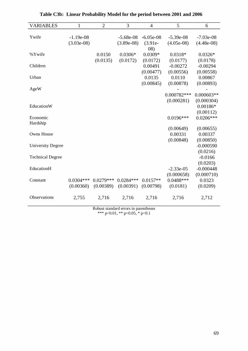
69

Table C3b: Linear Probability Model for the period between 2001 and 2006

VARIABLES 1 2 3 4 5 6

Ywife -1.19e-08 -5.68e-08 -6.05e-08 -5.39e-08 -7.03e-08 (3.03e-08) (3.89e-08) (3.91e-

08)

(4.05e-08) (4.48e-08)

%Ywife 0.0150 0.0306* 0.0309* 0.0318* 0.0326* (0.0135) (0.0172) (0.0172) (0.0177) (0.0178) Children 0.00491 -0.00272 -0.00294 (0.00477) (0.00556) (0.00558) Urban 0.0135 0.0110 0.00867 (0.00845) (0.00878) (0.00893) AgeW -

0.000782***

-

0.000603** (0.000281) (0.000304) EducationW 0.00186* (0.00112) Economic

Hardship 0.0196*** 0.0206***

(0.00649) (0.00655) Owns House 0.00331 0.00337 (0.00848) (0.00850) University Degree -0.000590 (0.0216) Technical Degree -0.0166 (0.0203) EducationH -2.33e-05 -0.000448 (0.000658) (0.000710) Constant 0.0304*** 0.0279*** 0.0284*** 0.0157** 0.0488*** 0.0323 (0.00360) (0.00389) (0.00391) (0.00798) (0.0181) (0.0209) Observations 2,755 2,716 2,716 2,716 2,716 2,712

Robust standard errors in parentheses *** p<0.01, ** p<0.05, * p<0.1

70

Table C4a: Linear Probability Model with Instrumental Variables for the period between

1996 and 2001, including Interactions of the Income variables with Total Household

Income Dummies.

(1)

VARIABLES Divorce

Ywife 1.55e-07

(1.98e-07)

Ywife*Dhy -1.14e-08

(8.55e-08)

%Ywife -0.0245

(0.0637)

Children -0.00836*

(0.00489)

Urban 0.0128

(0.00904)

AgeW -0.00101***

(0.000336)

EducationW 0.000264

(0.00127)

Economic Hardship 0.000449

(0.000835)

Owns House -0.000314

(0.00887)

EducationH -0.000175

(0.000977)

Constant 0.0618***

(0.0223)

Observations 2,431

R-squared 0.011

Standard errors in parentheses

*** p<0.01, ** p<0.05, * p<0.1

71

Table C4b: Linear Probability Model for the period between 2001 and 2006, including

Interactions of the Income variables with Total Household Income Dummies.

(1)

VARIABLES Divorce

Ywife 1.80e-07

(1.56e-07)

Ywife*Dhy -2.25e-07*

(1.34e-07)

%Ywife 0.00458

(0.0242)

Children -0.00293

(0.00558)

Urban 0.00834

(0.00891)

AgeW -0.000601**

(0.000302)

EducationW 0.00160

(0.00104)

Economic Hardship 0.0207***

(0.00654)

Owns House 0.00328

(0.00849)

EducationH -0.000376

(0.000711)

Constant 0.0333

(0.0205)

Observations 2,712

R-squared 0.011

Standard errors in parentheses

*** p<0.01, ** p<0.05, * p<0

Table E1: Variance-Covariance matrix for cases of Marital Disruption (if Y=1) for 1996-2001

Ywife %Ywife AgeW EducationW EducationH House EconHard

Ywife 1.00E+10

%Ywife 13923.1 0.048155

AgeW 314430 0.875879 135.145

EducationW 175942 0.222052 -4.78417 14.8409

EducationH 188071 0.09393 -7.24739 11.1445 27.8931

House 4961.28 -0.001914 0.28286 -0.143764 0.462939 0.218727

EconHard -17216.7 0.052872 0.427745 -3.52763 -4.17746 0.133962 12.5137

Table E2: Variance-Covariance matrix for cases of Marital Disruption (if Y=1) for 2001-2006

Ywife %Ywife AgeW EducationW EducationH House EconHard

Ywife 7.90E+09

%Ywife 20927.9 0.096362

AgeW 149402 0.776587 160.69

EducationW 93678.4 0.168513 -16.9383 13.2527

EducationH 157944 0.178764 -17.3209 8.12894 29.4781

House -888.642 -0.01311 1.32247 -0.087668 0.298046 0.173382

EconHard 1146.37 0.005948 -0.164957 0.019658 0.34188 0.035897 0.495726