Skewed Business Cycles

Sergio Salgado

⇤Fatih Guvenen

†Nicholas Bloom

‡

July 14, 2016

Preliminary and Incomplete. Comments Welcome.

Abstract

This paper studies how the distribution of the growth rate of macro- and micro-level variables changes over the business cycle. At the micro level, we use firm paneldata for more than 30 countries to show that skewness is strongly procyclical, drivenby a large left tail of negative growth rates during recessions. At the macro level,analyzing the growth rates of GDP and stock market returns, we find a similarphenomenon of procyclical skewness. These results are robust to different selectioncriteria, across countries, industries, and measures, suggesting that a wideningleft tail—and, consequently, a more negative skewness—is a basic stylized fact ofbusiness cycles.

⇤University of Minnesota; salga010@umn.edu.†University of Minnesota, FRB of Minneapolis, and NBER; guvenen@umn.edu‡Stanford University and NBER; nbloom@stanford.edu

1

1 Introduction

This paper studies the cyclicality of the distribution of the growth rate of firm-level and macroeconomic-level outcomes. In the prior literature, recessions have beencharacterized as a combination of a negative first-moment (mean) shock and a positivesecond-moment (uncertainty) shock.1 In this paper, we document that recessions are alsoaccompanied by negative third-moment (skewness) shocks which implies that, duringeconomic downturns, a subset of firms and countries does extremely badly, leading toa left tail of very negative outcomes. Consequently, the skewness of growth rates areprocyclical.

As a simple illustration, figure 1 displays the empirical density of the distributionof sales growth for a sample of Compustat firms. We show with (dashed) black linesthe density of the growth of sales between 2007q1 and 2008q1—just before the GreatRecession—while the (solid) red line is the density of the same variable between 2008q1and 2009q1—during the Great Recession. From left to right, the vertical lines are the10th and the 90th percentiles of each distribution. In the figure, both densities areadjusted to have zero mean and unit variance so one can directly compare the changesin the tails of the distribution. We can see clearly that, between 2008q1 and 2009q1, thedispersion of the sales growth distribution increased (the difference between the 90th and10th percentiles widened from 0.41 to 0.64). However, this increase in dispersion is drivenmostly by a widening of the left tail of the distribution, which in turn generates a decreasein the skewness. The drop in the skewness can be quantified using Kelly’s measure, whichis defined as the difference between the 90th to 50th percentiles spread, a measure ofdispersion in the right tail, and the spread between the 50th and the 10th percentiles, ameasure of dispersion in the left tail, divided by the distance between the 90th and the10th percentiles, which is a measure of the total dispersion of the distribution. Hence,for a distribution with a compressed upper half and a dispersed lower half (i.e., a left-tailskew), Kelly’s measure will be negative. We find that the skewness between these twoperiods dropped from 0.1 to –0.25. A value of 0.1 in 2007–2008 means that the righttail accounted for approximately 55% of the overall dispersion, whereas the lower tailaccounted for the remaining 45%, while the figure of –0.26 in the Great Recession meansthat the upper tail accounted for only 37% of the total dispersion and the lower tailaccounted for 63%. This is a rapid change in the relative sizes of each tail in just one

1See the literature surveyed in Bloom (2014).

1

Figure 1 – The Distribution of Sales Growth of US Public Firms BecameMore Negatively Skewed During The Great Recession

0.2

.4.6

.81

Den

sity

-2.5 -2 -1.5 -1 -.5 0 .5 1 1.5 2 2.5Normalized sales growth rate

2008q1 2009q1

Note: Figure 1 shows the empirical density of the growth rate of real quarterly sales in US dollars over a panel of publiclytraded firms with 25+ years of data from the Compustat/CRSP merged database. The growth rate is defined as arc-percentchange between quarter t and the same quarter of the following year.

year. Although the histogram in Figure 1 pertains to a short period covering just a fewquarters, we show that the same patterns highlighted here are robust across the entiresample we examine, both within the United States and in a large sample (more thanforty) of countries, across firm size categories, and across industries.

Our second empirical finding is that skewness is also strongly procyclical at themacroeconomic level. That is, within a country, the left tail of the distribution of ag-gregate measures of economic activity, such as GDP growth or stock market returns,stretches out and becomes thicker during recessions. Hence, at both the micro andmacro level, periods of low economic activity are characterized by an increase in theprobability of very large negative shocks at the firm and aggregate level.

Although the visual evidence provided in Figure 1 suggests that recessions are ac-companied by large, asymmetric changes in the mass of the distribution of growth rates,there are several reasons to perform a careful empirical and quantitative analysis forboth micro- and macro-level outcomes. First, it is important to disentangle the relativecontribution of the tails to the increase in dispersion that is observed during periods oflow economic activity, because this provides insight into the nature of the risk that firmsand individuals face during economic downturns. A symmetric increase in dispersion im-

2

plies that once we have controlled by changes in the mean, the risk is equally distributedbetween the tails (i.e., the probability of getting a very good outcome is similar to theprobability of getting a negative outcome of the same magnitude). However, the evi-dence that we present here suggests that, during recessions, the increase in dispersion isasymmetrically distributed with a higher weight on negative outcomes (i.e., an increasein the probability of observing very negative outcomes without an equivalent increase inthe probability of observing positive outcomes of the same magnitude). Second, to theextent that frictions and nonlinearities of individual decision rules are responsible for theprocyclicality of the skewness that we document in this paper, our evidence can serve asa way to evaluate competing mechanisms, because a model that is unable to account forthe large swings in the skewness of macro- and micro-level outcomes falls short in beinga good representation of the firm and macro-level dynamics that are observed duringa recession. Third, the large drop in economic activity that occurred during the GreatRecession has been difficult to account for in most of the commonly used macroeco-nomic models, which typically assume that macro and micro shocks follow a symmetricdistribution. This difficulty has motivated the surge in interest of studying models withnon-Gaussian shocks. Here, we present evidence that suggest that at the macro andmicro level, shocks depart largely from the typical Gaussian assumption.

This paper is related to several strands of literature. First, a growing body of researchstudies how macroeconomic models respond to non-Gaussian shocks. For instance, sev-eral authors have suggested that rare disasters—presumably arising from an asymmetricdistribution of shocks—are useful in explaining large fluctuations in economic activity,such as the Great Recession and account for the movement of real and financial vari-ables. Reviving the ideas introduced first by Rietz (1988), Barro (2006) uses a panel ofcountries to estimate the probability of large macroeconomic disasters and argues thatthese low-probability events can have substantial implications for asset pricing. Basedon this evidence, Gourio (2012) extends the standard dynamic stochastic general equi-librium model to include the probability of a small risk of a large negative shock. Hefinds that an increase in the probability of a disaster induces a contraction in output,employment, and especially, investment. Kilic and Wachter (2015) study the effects ofa disaster shock in the context of a search and matching model. They show that in-cluding disaster risk dramatically improves the performance of the model in terms ofunemployment dispersion, without resorting to large and volatile productivity shocks.We contribute to this literature in two ways. First, we show that tail risk is an intrinsic

3

part of the business cycle not only at the macroeconomic or sectoral level but also at themicroeconomic level. And second, the existing literature only considers how aggregatedisaster risk affects the decision of a representative firm, whereas in our case we con-sider an economy with a large number of heterogeneous firms subject to idiosyncraticproductivity shocks and aggregate risk in the form of shocks to the mean, variance, andskewness of the idiosyncratic productivity process.

Second, our paper relates directly to the study of the effects of uncertainty on firms’decisions. Bloom (2009) and Bloom et al. (2011), among others, show that an increase inthe dispersion of firms’ shocks can lead to a recession. The main propagation mechanismis a real-option channel: in the presence of fixed adjustment costs or irreversibility, anuncertainty shock makes firms more cautious and less willing to invest or hire becauseof the irreversible cost induced by these decisions, generating a drop in aggregate eco-nomic activity. Arellano et al. (2012) find that an increase in uncertainty can lead to areduction in employment and output in a model where firms are financially constrained,whereas Gilchrist et al. (2014) evaluate quantitatively which of these channels—financialfrictions or the wait-and-see behavior generated by the adjustment costs of capital andlabor—is more important in accounting for the empirical evidence. Our paper adds tothis literature in two ways: first, by documenting that the surge in dispersion observedduring recessions is related to an increase in the probability of large negative shocks,and second, by studying how asymmetric changes in risk could generate larger effects ineconomic activity than those found so far in the literature.

Finally, a growing literature analyzes the behavior of skewness in different contexts.For example, Guvenen et al. (2014) study the characteristics of individual earnings risk.They find that idiosyncratic shocks do not show any countercyclical variation in disper-sion but do exhibit strong procyclical skewness. That is, during recessions the upper tailof the earnings growth rates distribution collapses, while the left tail becomes thicker,implying a greater probability of observing large negative shocks. Busch et al. (2015)find similar results for the Sweden and Germany. Our analysis is in the same spiritas theirs but focuses on firm- and macro-level variables instead of workers’ wages. Ilutet al. (2014) study the asymmetric response of firms to news. Their analysis predictsthat the distribution of growth rates of employment should be negatively skewed, whichis confirmed by census data. We find similar results; however, our focus is the variabilityof the skewness of different firm and macro level outcomes and how it moves during thebusiness cycle. Decker et al. (2015) document the declining trend in the skewness of the

4

firm growth rate distribution in the United States. They find that this decline is dueto the drop in the number of young high-growth firms, especially during the post-2000period. Distante et al. (2013) characterize the distribution of firm-level growth using aquantile regression approach. As in our paper, they find strong procyclical skewness,whereas changes in the dispersion are of second-order importance.

2 Skewness over the Business Cycle

Our analysis is based on three large data sets. The first comprises firm-level paneldata across 44 countries that contain annual sales and annual employment informationbetween 1986 and 2014 obtained from the Bureau van Dijk’s Osiris data set. To ensurethat changes in the sample of firms do not bias our results, we focus on firms that arepresent in the sample for 10 years or more. Additionally, we restrict our sample tocountry/year cells with more than 100 firms, countries with at least 10 years of data,and years with 5 countries or more. We complement this data set with information onfirm-level stock prices obtained from the Global Compustat data set which contains dailystock price information for firms in 23 countries from 1986 to 2014.

Second, we extract a panel of firms from the CRSP-Compustat merged data set,which contains information on sales, employment, stock prices, and so on. Here we usedata on quarterly sales, daily stock prices, and annual employment from 1964 to 2014,and we restrict attention to a sample of firms with more than 25 years of data to avoidthe types of compositional issues identified in Davis and Haltiwanger (1995). The thirddata set is a panel of countries with information on quarterly GDP growth and dailyreturns data on a stock price index. Data on quarterly GDP are obtained from theOECD data sets, while daily stock price indexes are collected from the correspondingofficial source.

At the firm level, we calculate the growth rate of real variables (sales, employment,inventories, and others) as the log difference between two consecutive years, while dailystock returns are calculated as the log difference between two consecutive trading days.As an alternative measure of growth we use the arc percentage change between years(quarters) t and t + 1 (t + 4). The arc percentage change is defined for annual obser-vations as 2 (xi,t+1 � xi,t) / (xi,t+1 + xi,t). This measure has been popularized in the firmdynamics literature by Davis and Haltiwanger (1992) and has the advantage that, whileit is similar to a percentage change measure, it allows for entry/exit by including both

5

time t and t+ 1 measures in the denominator, one of which is allowed to be zero.

Our main measure of dispersion is the cross-sectional spread between the 90th and10th percentiles, denoted by P9010. In addition, we use the difference between the 90thand 50th percentiles, denoted by P9050, and the difference between the 50th and 10thpercentiles, denoted by P5010, as measures of dispersion in the upper and lower partsof the distribution. Finally, our preferred measure of skewness is the Kelly’s measure,which is defined as

KSK =(P90� P50)� (P50� P10)

P90� P102 [�1, 1].

Relative to the third standardized moment (which is another measure of skewness), thismeasure has the advantage of being robust to potential outliers. A negative value ofthis measure indicates that more than 50% of the total dispersion is coming from theleft tail and the skewness is negative. In the same way, a positive number indicates apositive skewed distribution, with more dispersion coming from the right tail. Clearly,this measure is equal to 0 if the distribution is symmetric, such as for the Normaldistribution.2

At the macro level, we calculate the dispersion and skewness of the growth rate ofGDP per capita and daily stock returns over a trailing window of three years. Hence,the moments of the distribution of macroeconomic variables in period t are calculatedusing only the information available up to that period. Additional details on the dataconstruction, selection criteria, and moment calculation can be found in Appendix A.

2.1 Cross-Country Evidence

Here we show that the within-country skewness of the growth rate of macro- andmicro-level variables is procyclical. First, we use firm-level data over a panel of countriesto show that the skewness at a microeconomic level positively comoves with the businesscycle. Figure 2 displays the empirical density of the distribution of the growth rateof annual real sales (in US dollars as of 2005) for a panel of firms spanning across 44countries over the period 1986 to 2013.3

To construct the figure, we start by pooling all the firms available in the panel andthen normalize the distribution to have zero mean and unit variance. The solid red line

2Other robust measures of skewness can be found in Kim and White (2004).3Table A.3 in Appendix A shows the number of years and firm-level data available for each of the

countries in the sample.

6

is the density of sales growth during recession periods, where a recession is defined as ayear in which the annual growth rate of GDP is in the first decile of the country-specificGDP growth distribution.4 The dashed black line is the density of sales growth duringexpansion periods (years in which GDP growth is above the first decile). The verticalsolid (dashed) lines, from left to right, are the 10th, 50th, and 90th percentiles of thedistribution of sales growth during recession (expansion) periods.

First, observe that the median of the distribution drops during recessions (in this case,from –0.03 to –0.07), and second, the dispersion increases as the difference between the90th and the 10th percentiles of the distribution widens (from 1.73 to 1.95, an increaseof 22 log points). This increase, however, is mostly attributable to a change in the lefttail of the distribution that stretches out, with a corresponding increase in the spreadbetween the 50th and 50th percentiles (from 0.77 to 0.94, or an increase of 17 log points)which is almost three times as large as the increase in the spread between the 90th and50th percentiles (it increases from 0.96 to 1.02, or 6 log points). A consequence of thisuneven increase in dispersion is a large drop in the skewness: Kelly’s measure drops from0.10 to 0.04.

These two related business cycle facts—the increase of dispersion below the medianand the drop in skewness—are not limited to the sales growth distribution but, as weshow here and discuss in the following sections, they hold for several other variables, atboth firm and aggregate level, within different countries, and across different industries.The first evidence of the generality of our results is shown in Figure 3, which is based onan unbalanced panel of countries for which we have firm- and aggregate-level data.

To construct the graph, each country/period is placed into a bin based on the decilesof the country-specific distribution of the growth rate of annual GDP with bins, from 1to 10, where 1 is the lowest decile of growth and 10 is the highest decile. So, for example,for the United States, bin 1 is for growth rates below –1.2%, bin 2 is for growth ratesbetween –1.2% and 0.1% and so on, whereas for the United Kingdom, the first bin is forgrowth rates below –1.1%, the second bin is for growth rates between –1.1% and 0.2%,and so on. The skewness measure plotted for each bin are averages over each country-year in the bin. In each decile, we plot the Kelly’s measure of skewness for four differentdistributions—with each measure normalized to a mean 0 and standard deviation of 1:the within-country cross-sectional distribution of firm-level real sales growth, the within-

4This particular definition of a recession period allows us to have uniform criteria across countriesand samples.

7

Figure 2 – The Distribution of Firm Sales Growth Rates Becomes MoreNegatively Skewed During Recessions, Pooled Panel of 44 Countries

0.2

.4.6

.81

Den

sity

-2.5 -2 -1.5 -1 -.5 0 .5 1 1.5 2 2.5Normalized sales growth rate

Expansions Recessions

Note: Figure 2 shows the the empirical density of the growth rate of annual sales in US dollars over a panel of firms in44 countries between 1986 and 2013. To construct the figure, we first adjust the sales growth distribution within eachcountry to have mean zero and unit variance. Then, the red solid line is the empirical density over all the observationsof firms during recession periods (77,137 observations) while the black line pools all the observations during non-recessionperiods (418,256 observations).

country cross-sectional distribution of firm-level daily stock returns, the within-countrydistribution of the growth rate of GDP, and the within country distribution of the dailyreturns of a stock price index.

For all these variables, the skewness is low when country growth is lower, particularlywhen the growth rate of GDP is in its lowest decile, which is typically during a recession.This highlights the generality of the link between recessions and skewness. In a similarway, we can ask if the dispersion of the distribution of sales, stock returns, and GDPgrowth is countercyclical, as has been previously documented (see Bloom (2009) and thesubsequent literature). This is shown in Figure 4, which displays the spread of the 90thto the 10th percentiles in each of the distributions of micro- and macro-level outcomes.As expected, the P9010 is countercyclical, staying well above the mean during periodsof low economy activity and falling fast as we move to higher deciles of the GDP growthdistribution. For further evidence, Figure A.3 in Appendix B shows a similar decliningtrend for the dispersion on the left tail measured by the P5010.

Table I evaluates more systematically the relationship of our micro (firm-level) mea-

8

Figure 3 – Skewness of Growth Rates is Procyclical, Pooled Panel of 44Countries

−3−2

−10

12

Skew

ness

: Kel

ly(n

orm

aliz

ed to

mea

n 0,

SD

1)

1 2 3 4 5 6 7 8 9 10GDP growth deciles

Micro Sales Micro ReturnsMacro GDP Macro Returns

Note: Figure 3 is based on annual, quarterly, and daily data for a sample of developed and developing countries over theperiod 1985 to 2013. Each country-year cell is placed into a bin based on the decile of the country-specific distribution ofthe growth rate of annual real GDP, where 1 is the lowest decile of growth and 10 is the highest. The skewness measuresshown are averages for each country-year in the bin. Each decile shows four different measures of skewness, two macro,the KSK of the growth rate of GDP growth and the KSK of daily returns of a stock price index, and two micro, theKSK of the within-country cross sectional distribution of firm-level sales growth and the KSK of the within- countrycross sectional distribution of firm-level daily stock returns. Each measure has been normalized to mean 0 and standarddeviation 1.

sures of skewness and dispersion with the economic activity. In columns (1) to (4) weregress the growth rate of GDP of country i in period t, on different moments of thecross-sectional distribution of sales growth calculated over all the firms in country i inperiod t and a full set of country and year fixed effects. In particular, we run the followinglinear specification:

g

GDPit = �i + �t + �xit + ✏it,

where xit is a cross-sectional moment of the sales growth distribution of firms in countryi during period t. Column (1) of Table I shows that the dispersion of firms’ sales growthis negatively correlated with the country’s business cycle. However, given the evidencein figure 2, one might suspect that the increase in dispersion comes mostly from changesin the left tail of the distribution whereas the right tail does not change much with theeconomic cycle. Columns (2) and (3) show that this is indeed the case, because the

9

Figure 4 – Dispersion of Growth Rates is Countercyclical, Panel of 44Countries

−10

12

3

Dis

pers

ion:

P90−P

10(n

orm

aliz

ed to

mea

n 0,

SD

1)

1 2 3 4 5 6 7 8 9 10GDP growth deciles

Micro Sales Micro ReturnsMacro GDP Macro Returns

Note: Figure 4 is based on annual, quarterly, and daily data for a sample of developed and developing countries over theperiod 1985 to 2013. Each decile shows four different measures of dispersion, two macro, the P9010 of the growth rateof GDP growth and the P9010 of daily returns of a stock price index, and two micro, the P9010 of the within-countrycross sectional distribution of firm-level sales growth and the P9010 of the within–country cross sectional distribution offirm–level daily stock returns. See notes in Figure 3 for additional details.

within-country spread between the 50th and the 10th percentiles is negatively correlatedwith the GDP growth whereas the gap between the 90th and 50th percentiles is onlyweakly correlated with the cycle.

Finally, column (4) shows the main result of this section: we find that the within-country skewness of the sales growth distribution is positively correlated with the businesscycle. We find a positive and statistically significant coefficient of 0.028 (a t-statistic of3.34). This implies that a drop in the skewness of 0.36, which is equal to a drop of twostandard deviations in the sample, is associated with a drop of 1% in the growth rate ofGDP.5

In columns (5) to (8) we provide additional firm-level results considering the cross-sectional moments of the distribution of daily stock returns. In column (5) we examinethe cross-sectional dispersion, which reflects the volatility of news about overall firmperformance. Here again we find that dispersion is countercyclical, similar to previousresults (see, for instance, Campbell et al. (2001)). We also find a positive and statisticallysignificant relation between the business cycle and the skewness of the distribution of

5This drop in the Kelly’s measure of skewness of 0.36 is also similar to what we observe in a typicalUS recession. See Figure A.1 in Appendix B for further details.

10

daily returns.

In Table II we report an additional set of results on the relation between dispersionand skewness and the business cycle but now using macroeconomic (rather than firm-level) data. In column (1) of Table II, we regress the growth rate of quarterly GDP on theP9010 of the GDP growth distribution, calculated over a trailing window of three yearsof data (we use a trailing window to avoid using future data to account for current GDPgrowth). Here again, we find strong countercyclicality of dispersion. Comparing columns(2) and (3), we find that the the countercyclicality at the left tail of the distribution ismuch stronger than the cyclicality at the right tail. Consequently, in column (4), wefind a strong and positive relation between the business cycle and the skewness of thegrowth rate of GDP. This implies that recessions are periods characterized by unusuallylarge drops in economic activity, which echoes the work of Barro (2006), Gourio (2012),and the “disaster” shocks literature. In line with our previous results, the skewness ofthe daily returns in the stock market is positively correlated with the business cycle, asshown in column (8) of Table II.

In summary, in this section we have shown that slowdowns in economic activityare accompanied by large declines in the skewness of the within-country distributionof macro- and microeconomic outcomes. The skewness dives because the left tail ofthe distribution expands during recessions as a disproportionate number of firms andcountries get hit with large negative shocks.

In the following sections, we provide evidence of the robustness of our results, showingthat they hold if we focus on the US economy only, when we consider different industries,and for different firm-level outcomes.

2.2 Results for the United States

In this section, we provide the first robustness check of our results using macro- andfirm-level data for the US economy. Focusing on the United States allows us to compareour results with the existing literature more directly and study a larger set of firm-leveloutcomes, which are not available for the cross-country panel of firms. First, similarlyto the previous section, in Figure 5 we plot the empirical density of the distribution ofthe growth rate of real sales for recession and expansion periods for a sample of publiclytraded firms. In the figure, we pool all the firm-quarter observations from 1970 to 2014,and we normalize the distribution to have zero mean and unit variance. Then, the solid

11

Tab

leI

–W

ithi

n-C

oun

try

Dis

pers

ion

and

Skew

ness

of

Mic

roLev

elO

utco

mes

(1)

(2)

(3)

(4)

(5)

(6)

(7)

(8)

Dependent

Variable:

Grow

th

Rate

of

GD

Pw

ithin

each

country

Distribution:

Grow

th

Rate

of

Sales

Daily

Stock

Returns

P9010

i,t

–0.017**

–0.243***

(0.008)

(0.085)

P5010

i,t

–0.048**

–0.556***

(0.019)

(0.184)

P9050

i,t

0.004

–0.366***

(0.014)

(0.141)

KSK

i,t

0.028***

0.064***

(0.008)

(0.018)

R2

0.51

00.

523

0.50

60.

523

0.71

70.

721

0.71

30.

714

N76

076

076

076

017

9317

9317

9317

93Fr

eq.

Ann

ual

Ann

ual

Ann

ual

Ann

ual

Qua

rter

lyQ

uart

erly

Qua

rter

lyQ

uart

erly

Yea

rs19

85-2

012

1985

-201

219

85-2

012

1985

-201

219

86-2

014

1986

-201

419

86-2

014

1986

-201

4U

nder

.Sa

mpl

e50

5,73

550

5,73

550

5,73

550

5,73

572

,799

,363

72,7

99,3

6372

,799

,363

72,7

99,3

63C

ount

ry-T

ime

FEY

esY

esY

esY

esY

esYes

Yes

Yes

Clu

ster

ing

Cou

ntry

Cou

ntry

Cou

ntry

Cou

ntry

Cou

ntry

Cou

ntry

Cou

ntry

Cou

ntry

Not

e:E

ach

colu

mn

repo

rts

the

resu

lts

from

aco

untr

y-ye

arO

LS

pane

lre

gres

sion

incl

udin

ga

full

set

ofco

untr

yan

dti

me

fixed

effec

ts(y

earl

yfix

edeff

ects

for

colu

mns

(1)

to(4

)an

dqu

arte

rly

fixed

effec

tsfo

rco

lum

ns(5

)to

(8))

.In

colu

mns

(1)

to(4

),th

ede

pend

ent

vari

able

isth

egr

owth

rate

ofre

alG

DP

inU

Sdo

llars

asof

2005

ofco

untr

yi

betw

een

year

tan

dt+

1,

and

betw

een

quar

tert

and

t+

4in

colu

mns

(5)

to(8

).In

colu

mns

(1)

to(4

),th

ein

depe

nden

tva

riab

les

are

mom

ents

ofth

ew

ithi

n-co

untr

ycr

oss-

sect

iona

ldi

stri

buti

onof

sale

sgr

owth

for

asa

mpl

efir

ms

inco

untr

yi

inpe

riod

tfr

omth

eO

siri

sda

taba

se.

To

calc

ulat

eth

em

omen

ts,

inea

chco

untr

yw

edr

opal

lth

efir

ms

wit

hle

ssth

an10

year

sof

data

,w

edr

opea

chco

untr

y-ye

arce

llw

ith

less

than

100

firm

s,w

edr

opal

lco

untr

ies

wit

hle

ssth

an10

year

sof

data

,an

dw

edr

opal

lth

eye

ars

wit

hle

ssth

an5

coun

trie

s.In

colu

mns

(5)

to(8

),th

ein

depe

nden

tva

riab

les

are

cros

sse

ctio

nalm

omen

tsof

the

wit

hin-

coun

try

cros

sse

ctio

nald

istr

ibut

ion

ofda

ilyst

ock

retu

rns

for

asa

mpl

eof

firm

sin

coun

tryiin

peri

odtfr

omG

loba

lCom

pust

at.

To

calc

ulat

eth

em

omen

ts,i

nea

chco

untr

yw

eco

nsid

erfir

ms

wit

hap

prox

imat

ely

10ye

ars

ofda

ta(m

ore

than

2000

trad

ing

days

),an

dw

eal

soco

nsid

erqu

arte

r-co

untr

yce

llsw

ith

mor

eth

an10

0fir

ms,

and

quar

ters

wit

hda

tafr

omat

leas

t5

coun

trie

s.St

anda

rder

rors

,sh

own

inpa

rent

hese

sbe

low

the

poin

tes

tim

ates

,ar

ecl

uste

red

atth

eco

untr

yle

vel.

⇤⇤⇤

deno

tes

1%,⇤⇤

deno

tes

5%,an

d⇤

deno

tes

10%

sign

ifica

nce,

resp

ecti

vely

.

12

Tab

leII

–W

ithi

n-C

oun

try

Dis

pers

ion

and

Skew

ness

of

Mac

roLev

elO

utco

mes

(1)

(2)

(3)

(4)

(5)

(6)

(7)

(8)

Dependent

Variable:

Grow

th

Rate

of

GD

Pw

ithin

each

country

Distribution:

Grow

th

Rate

of

GD

PD

aily

Returns

of

Stock

Price

Index

P9010

i,t

–0.1

50**

*–0

.253

***

(0.0

48)

(0.0

81)

P5010

i,t

–0.1

94**

*–0

.620

***

(0.0

59)

(0.1

57)

P9050

it–0

.165

*–0

.362

**

(0.0

88)

(0.1

59)

KSK

i,t

0.00

5**

0.04

7***

(0.0

02)

(0.0

11)

R2

0.65

00.

650

0.64

20.

641

0.72

30.

723

0.72

20.

723

N57

4657

4657

4657

4628

7828

7828

7828

78Fr

eq.

Qua

rter

lyQ

uart

erly

Qua

rter

lyQ

uart

erly

Qua

rter

lyQ

uart

erly

Qua

rter

lyQ

uart

erly

Yea

rs19

70-2

014

1970

-201

419

70-2

014

1970

-201

419

70-2

014

1970

-201

419

70-2

014

1970

-201

4C

ount

ry-Q

trFE

Yes

Yes

Yes

Yes

Yes

Yes

Yes

Yes

Clu

ster

ing

Cou

ntry

Cou

ntry

Cou

ntry

Cou

ntry

Cou

ntry

Cou

ntry

Cou

ntry

Cou

ntry

Not

e:E

ach

colu

mn

repo

rts

the

resu

lts

from

aco

untr

y-qu

arte

rO

LS

pane

lre

gres

sion

incl

udin

ga

full

set

ofco

untr

yan

dqu

arte

rfix

edeff

ects

.In

each

colu

mn,

the

depe

nden

tva

riab

leis

the

grow

thra

teof

real

GD

Pin

US

dolla

rsas

of20

05of

coun

tryi

betw

een

quar

tert

and

the

sam

equ

arte

rof

the

next

year

.T

hein

depe

nden

tva

riab

les

inco

lum

ns(1

)to

(4)

are

mom

ents

ofth

ew

ithi

n-co

untr

ydi

stri

buti

onof

the

grow

thra

teof

quar

terl

yG

DP.

The

inde

pend

ent

vari

able

sin

colu

mns

(5)

to(8

)ar

em

omen

tsof

the

dist

ribu

tion

ofda

ilyre

turn

sof

ast

ock

pric

ein

dex

ofco

untr

yi.

The

n,to

calc

ulat

eth

em

omen

tsof

the

GD

Pgr

owth

dist

ribu

tion

(dai

lyre

turn

s)in

quar

tert,

we

pool

allt

heob

serv

atio

nsbe

twee

nqu

arte

rst�

12

andt

tom

ake

ato

talo

f13

quar

ters

.St

anda

rder

rors

,sho

wn

inpa

rent

hese

sbe

low

the

poin

tes

tim

ates

,ar

ecl

uste

red

atth

eco

untr

yle

vel.

⇤⇤⇤

deno

tes

1%,⇤

⇤de

note

s5%

,and

⇤de

note

s10

%si

gnifi

canc

e,re

spec

tive

ly.

13

Figure 5 – The Distribution of Firm Sales Growth Rates Becomes MoreNegatively Skewed During Recessions, United States

0.2

.4.6

.8D

ensi

ty

-2.5 -2 -1.5 -1 -.5 0 .5 1 1.5 2 2.5Normalized sales growth rate

Expansions Recessions

Note: Figure 5 shows the empirical density of the growth rate of real quarterly sales in US dollars over a panel of publiclytraded firms with 25+ years of data between 1970 and 2014. The red line is the empirical density over all the observationsof firms during recession periods (18 quarters and 24,300 firm-quarter observations) while the black line pools all theobservations for non-recession periods (162 quarters and 235,092 firm-quarter observations).

red line shows the empirical density of the sales growth distribution during recessionperiods. Here we define a recession period as a quarter in which the growth rate of GDPis in the first decile of the quarterly GDP growth distribution.

On the other hand, the dashed black line shows the density of the sales growthdistribution during expansion periods. The vertical solid (dashed) lines, from left toright, are the 10th, 50th, and 90th percentiles of the distribution of sales growth duringrecession (expansion) periods.6 Here the differences between recession and expansionperiods are even larger than in the previous section: the spread between the 90th and10th percentiles increases (from 1.62 to 2.09, an increase of 47 log points) but this increaseis largely explained by a change in the left tail of the distribution, because the differencebetween the 90th and 50th percentiles rises by only 6 log points (0.86 to 0.92) whilethe spread between the 50th and 10th increases by 41 log points (0.77 to 1.18). Hence,Kelly’s measure of skewness drops from 0.04 to –0.12.

6The results do not depend on this particular selection of recession periods and remain the same ifwe use a more standard definition such as the NBER dates.

14

Figure 6 – Skewness of Growth Rates is Procyclical, United States

−2−1

01

2

Skew

ness

: Kel

ly(n

orm

aliz

ed to

mea

n 0,

SD

1)

1 2 3 4 5 6 7 8 9 10GDP growth deciles

Micro Sales Micro ReturnsMacro GDP Macro Returns

Note: Figure 6 is based on quarterly firm-level sales data, firm-level daily stock returns, quarterly GDP growth, and dailyreturns of the S&P500 index over the period 1970 to 2014. Each quarter is placed into a bin based on the decile of theannual growth rate of quarterly GDP, with bins from 1 to 10, where 1 is the lowest decile growth and 10 is the highest.So for example, bin 1 is growth rates below 0, corresponding to periods such as 1980q3, with a growth rate of -1.6% or2009q1, with a growth rate of -3.5%. The skewness measures plotted for each bin are averages for each quarter in thebin. Each decile shows four measures of skewness, two macro, the KSK of the growth rate of GDP and the KSK ofdaily returns of the S&P500, and two micro, the KSK of the distribution of quarterly sales growth and the KSK of thedistribution of daily stock returns, with each measure normalized to a mean of 0 and standard deviation of 1.

Next, we proceed in a similar fashion as before and construct the US time series ofdispersion and skewness at both the micro and macro level, and then average differentperiods according to their position in the quarterly GDP growth distribution. Figure 6shows that skewness is strongly procyclical at both the macro and micro level, stayingwell below the mean at low levels of GDP growth and increasing almost monotonicallyfor all our measures as we move to higher levels of economic activity. Figure 7 showshow our preferred measure of dispersion, the P9010, changes across different deciles ofthe distribution of quarterly GDP growth. Here we also find countercyclical dispersionat both the macro and micro level. Figure A.4 in Appendix B complements these resultsby showing how the dispersion in the left and right tails changes across different decilesof the GDP growth distribution.

The strong procyclicality of macro- and micro-level outcomes in the United States isalso evident in our regression results. First, columns (1) to (4) in Table III show a seriesof regressions for the growth rate of quarterly GDP per capita on different measures of

15

Figure 7 – Dispersion of Growth Rates is Countercyclical, United States

−2−1

01

2

Dis

pers

ion:

P90

− P

10(n

orm

aliz

ed to

mea

n 0,

SD

1)

1 2 3 4 5 6 7 8 9 10GDP growth deciles

Micro Sales Micro ReturnsMacro GDP Macro Returns

Note: Figure 7 is based on firm-level quarterly sales data, firm-level daily stock returns, quarterly GDP growth for theUnited States, and daily returns of the S&P500 index over the period 1970 to 2014. Each decile shows four measuresof dispersion, two macro, the P9010 of the distribution of the growth rate of GDP and the P9010 of the distributiondaily returns of the S&P500, and two micro, the P9010 of the distribution of quarterly sales growth and the P9010 of thedistribution of daily stock returns, with each measure normalized to a mean of 0 and standard deviation of 1. See notesin Figure 6 for additional details.

dispersion and skewness of the distribution of sales growth, a constant, and a linear trend.Column (1) shows the expected strong and negative relation between economic activityand dispersion, while columns (2) and (3) show that most of the countercyclicality ofdispersion is accounted for by the left tail of the distribution of sales growth. Thecorrelation between the P5010 is negative and highly significant, while the P9050, ourmeasure of dispersion above the median, is positively correlated with GDP growth.

Given these asymmetric changes in the tails of the distribution over the business cycleand our previous results, we expect to find a strong and positive correlation between theskewness of the growth rate of sales and the growth rate of GDP, as shown in column (4).A coefficient of 0.08 indicates that a decrease in the skewness of 30%, similar to whatwas observed during the Great Recession, is associated with a decline in GDP of 2.4%,which is a very large number considering that the standard deviation of GDP growth isaround 2.2%. As we show in Appendix B, these results are also evident when we lookdirectly to the time series of dispersion and skewness (Appendix figures A.1 and A.2),when we relax the selection criteria to allow firms with 10 or more years of data (Table

16

A.6), or when we consider a strictly balanced panel of firms (Table A.7). Finally, column(8) examines the relation between the skewness of the stock returns and the businesscycle, and again, we find that it is strongly procyclical.

In addition to the evidence using micro-level data, in Table IV we report a set ofresults using macroeconomic series. In columns (1) to (4) we run a set of regressions ofthe growth rate of quarterly GDP on different moments of the distribution of the growthrate of GDP. Columns (5) to (8) do the same but use moments of the distribution of dailyreturns of the S&P500. Here again, we find countercyclical dispersion and procyclicalskewness.

3 Robustness

In this section, we discuss several robustness checks that show the generality of theresults presented in the previous sections.

3.1 Grouping Countries by Income

First, we show that our results remain robust if we separate our sample into developedand developing countries as measure by their level of income per capita. Figure A.8 inAppendix B displays the average measure of skewness within deciles of the GDP growthdistribution for these two groups. We classify as developed all the countries in the upperhalf of the distribution of GDP per capita in the year 2000 (in US dollars as in 2005),and the rest are classified as developing countries. We find that skewness at both themicro and macro level is procyclical within both groups. Dispersion is countercyclical asshown in Figure A.9.

3.2 Industry

We can gain additional insight by desegregating our sample of US firms by industry.For consistency with the previous results, we use the sample of firms with more than25 years of data and separate firms in seven broad categories based on the SIC codesreported in CRSP/Compustat. Table A.8 in Appendix B shows the number of firm-quarter observations in each of the sectors and a set of cross sectional moments of thesales growth distribution. To study whether our main results hold at the industry level,we first look at the same set of plots discussed in the previous section. We first constructtime series of skewness and dispersion of the sales growth distribution and daily stock

17

Tab

leII

I–

Dis

pers

ion

and

Skew

ness

of

Mic

roLev

elO

utco

mes

inth

eU

nite

dSt

ates

(1)

(2)

(3)

(4)

(5)

(6)

(7)

(8)

Dependent

Variable

Grow

th

Rate

of

GD

P

Distribution

Grow

th

Rate

of

Sales

Daily

Stock

Returns

P9010

t–0

.056

**–0

.262

***

(0.0

22)

(0.0

95)

P5010

t–0

.157

***

–0.7

06**

*(0

.033

)(0

.208

)

P9050

t0.

067*

*–0

.263

(0.0

33)

(0.1

83)

KSK

t0.

078*

**0.

095*

**(0

.013

)(0

.023

)

N20

020

020

020

020

020

020

020

0Fr

eque

ncy

Qua

rter

lyQ

uart

erly

Qua

rter

lyQ

uart

erly

Qua

rter

lyQ

uart

erly

Qua

rter

lyQ

uart

erly

Und

er.

Sam

ple

266,

485

266,

485

266,

485

266,

485

31,2

30,0

3631

,230

,036

31,2

30,0

3631

,230

,036

Yea

rs19

64-2

013

1964

-201

319

64-2

013

1964

-201

319

64-2

013

1964

-201

319

64-2

013

1964

-201

3

Not

e:E

ach

colu

mn

repo

rts

adi

ffere

ntti

me

seri

esO

LS

regr

essi

onin

clud

ing

aco

nsta

ntan

da

linea

rtr

end.

Inea

chco

lum

n,th

ede

pend

ent

vari

able

isth

egr

owth

rate

ofre

alG

DP

per

capi

tabe

twee

nqu

arte

rt

and

the

sam

equ

arte

rof

the

follo

win

gye

ar.

The

inde

pend

ent

vari

able

sin

colu

mns

(1)

to(4

)ar

ecr

oss-

sect

iona

lm

omen

tsof

the

dist

ribu

tion

ofth

egr

owth

rate

ofqu

arte

rly

sale

sfo

ra

sam

ple

ofC

ompu

stat

firm

sw

ith

25or

mor

eye

ars

ofda

ta(1

00qu

arte

rs).

The

inde

pend

ent

vari

able

sfr

omco

lum

ns(5

)to

(8)

are

cros

s-se

ctio

nalm

omen

tsof

the

dist

ribu

tion

ofda

ilyre

turn

sfo

ra

sam

ple

ofC

ompu

stat

firm

sw

ith

25or

mor

eye

ars

ofda

ta(5

000

trad

ing

days

).To

calc

ulat

eth

ecr

oss-

sect

iona

lm

omen

tsof

the

sale

sgr

owth

dist

ribu

tion

(dai

lyre

turn

s)in

quar

tert,

we

pool

allth

eob

serv

atio

nsof

quar

tert.

New

ey-W

est

stan

dard

erro

rsar

eap

plie

din

each

colu

mn

toco

ntro

lfor

auto

corr

elat

ion

(max

of1

lag)

.⇤⇤⇤

deno

tes

1%,⇤

⇤de

note

s5%

,and

⇤de

note

s10

%si

gnifi

canc

e,re

spec

tive

ly.

18

Tab

leIV

–D

ispe

rsio

nan

dSk

ewne

ssof

Mac

roLev

elO

utco

mes

inth

eU

nite

dSt

ates

(1)

(2)

(3)

(4)

(5)

(6)

(7)

(8)

Dependent

Variable

Grow

th

Rate

of

GD

P

Distribution

Grow

th

Rate

of

GD

PD

aily

Returns

of

Stock

Price

Index

P9010

t–0

.141

–0.7

71**

*(0

.093

8)(–

3.03

)

P5010

t–0

.328

**–1

.888

***

(0.1

31)

(–4.

08)

P9050

t0.

092

–0.8

74(0

.168

)(–

1.59

)

KSK

t0.

011*

*0.

123*

**(1

.98)

(4.8

3)

N20

420

420

420

420

420

420

420

4Fr

eque

ncy

Qua

rter

lyQ

uart

erly

Qua

rter

lyQ

uart

erly

Qua

rter

lyQ

uart

erly

Qua

rter

lyQ

uart

erly

Yea

rs19

64-2

014

1964

-201

419

64-2

014

1964

-201

419

64-2

014

1964

-201

419

64-2

014

1964

-201

4

Not

e:E

ach

colu

mn

repo

rts

adi

ffere

ntti

me

seri

esO

LS

regr

essi

onin

clud

ing

aco

nsta

ntan

da

linea

rtr

end.

Inea

chco

lum

n,th

ede

pend

ent

vari

able

isth

egr

owth

rate

ofre

alG

DP

indo

llars

betw

een

quar

tert

and

the

sam

equ

arte

rof

the

follo

win

gye

ar.

The

inde

pend

ent

vari

able

sin

colu

mns

(1)

to(4

)ar

em

omen

tsof

the

dist

ribu

tion

ofth

egr

owth

rate

ofG

DP.

The

inde

pend

ent

vari

able

sin

colu

mns

(5)

to(8

)ar

em

omen

tsof

the

dist

ribu

tion

ofda

ilyre

turn

sof

the

S&P

500

inde

x.To

calc

ulat

eth

em

omen

tsof

the

GD

Pgr

owth

dist

ribu

tion

(dai

lyre

turn

s)in

quar

tert

we

pool

allt

heob

serv

atio

nsbe

twee

nqu

arte

rst�

12

andt

tom

ake

ato

talo

f13

quar

ters

ofda

ta.

New

ey-W

est

stan

dard

erro

rsar

eap

plie

din

each

colu

mn

toco

ntro

lfor

auto

corr

elat

ion

(max

of1

lag)

.⇤⇤⇤

deno

tes

1%,⇤

⇤de

note

s5%

,and

⇤de

note

s10

%si

gnifi

canc

e,re

spec

tive

ly.

19

returns. Then, we separate the sample in bins depending on the deciles of the growthrate of aggregate GDP, and finally we plot the within-industry average of the measuresof skewness and dispersion for each of the bins. As shown in Figure A.5 in AppendixB, the skewness measures of the within-industry distribution of sales growth and stockreturns both increase as one moves from lower to higher deciles of the distribution ofGDP growth, while the dispersion (Figure A.6 in Appendix B) decreases as one movesto higher levels of economic activity.

To complete the analysis, we run a set of industry panel regressions in which thedependent variable is the median value of the distribution of sales growth across all firmsin industry i in quarter t, denoted by P50it, while the independent variables are within-industry measures of dispersion and skewness of the distribution of sales growth or dailystock returns, a full set of industry fixed effects, and a quadratic in time. To be moreprecise, the regression specification that we run is

P50it = �i + ↵1t+ ↵2t2 + �xit + ✏it.

As shown in more detail in Table A.9 in Appendix B, the skewness of the within-industrydistribution of sales growth is positively and strongly correlated with the industry busi-ness cycle. We find similar results when we consider moments of the distribution stockreturns. So, at both the aggregate and industry level, slowdowns are associated with adecrease in the cross-sectional skewness of the sales growth and stock returns distribu-tions.

3.3 Entry and exit

How much would our results change if we consider the entry and exit of firms? Inorder to study this, we use the arc percentage measure of growth, which takes intoaccount entry and exit. In particular, upon entry, this measure of growth is equal to2, while in the period of exit it is equal to –2. Then we recalculate the same set ofcross-sectional moments for this measure of growth over the same sample of firms with10 or more years of data. Table A.12 repeats the analysis of Table III, but in this casethe cross-sectional measures of dispersion and skewness take into account the entry andexit of firms. Here again we find procyclicality of skewness.

20

3.4 Employment, profits and inventories moments

Additionally, we can ask whether the skewness of other firm-level outcomes, such asthe growth rate of employment, profits, or the value of inventories, is also procyclical.To see if this is the case, we run a series of regressions in which the dependent variableis the growth rate of GDP per capita and the independent variable is the cross sectionalskewness of the distribution of growth rates of annual employment, quarterly inventories,or quarterly profits. As shown in Table A.10 in Appendix B, we robustly find that theskewness of these firm-level outcomes drops during recession periods.

3.5 Firm size

Is the cyclical behavior of the skewness of sales growth different for small and largefirms? To answer this question, we use a sample of Compustat/CRSP firms with 10 ormore years of data.7 Since publicly traded firms are typically large, we split the sampleaccording to industry-specific size groups. That is, in each year, we consider as small allthe firms in the first quartile of the industry-specific distribution of employment. Firmsof medium size are those in the second quartile, and so on. Then we pool together all thefirms in the size category and calculate different moments of the sales growth distributionacross all the firms in the group. As we show in Figure A.7 in Appendix B, variations inthe skewness of the sales growth distribution are quite similar across different firm-sizeclasses. This is also evident from the regression results shown in Table A.11 in appendixB.

Thus in summary, it seems that the procyclicality of the skewness of the distributionof firm-level outcomes is a robust phenomenon, which is evident if we look at differentgroups of countries, within firms of different sizes or industries, and for several firm-leveloutcomes.

4 Conclusions

This paper studies how the distribution of the growth rate of macro- and micro-levelvariables changes over the business cycle. At the micro level, we use firm panel datafor more than 30 countries to show that skewness is strongly procyclical, driven by alarge left tail of negative growth rates during recessions. At the macro level, analyzing

7The results are similar when we use a sample of firms with 25 years or more, but using this dataset significantly reduces the variability between firm-size groups.

21

the growth rates of GDP and stock market returns, we find a similar phenomenon ofprocyclical skewness. These results are robust to different selection criteria, across coun-tries, industries, and measures, suggesting that a widening left tail—and, consequently,a more negative skewness—is a basic stylized fact of business cycles.

22

References

Arellano, C., Bai, Y. and Kehoe, P. J. (2012). Financial Frictions and Fluctuationsin Volatility. Staff Report 466, Federal Reserve Bank of Minneapolis.

Barro, R. J. (2006). Rare disasters and asset markets in the twentieth century. Quar-terly Journal of Economics, 121 (3), 823–866.

Bloom, N. (2009). The Impact of Uncertainty Shocks. Econometrica, 77 (3), 623–685.

— (2014). Fluctuations in Uncertainty. Journal of Economic Perspectives, 28 (2), 153–76.

—, Floetotto, M., Jaimovich, N., Saporta-Eksten, I. and Terry, S. J. (2011).Really Uncertain Business Cycles. Working paper, Stanford University.

Busch, C., Domeij, D., Guvenen, F. and Madeira, R. (2015). Higher-Order IncomeRisk and Social Insurance Policy Over the Business Cycle. Working paper, Universityof Minnesota.

Campbell, J. Y., Lettau, M., Malkiel, B. and Xu, Y. (2001). Have individualstocks become more volatile? an empirical exploration of idiosyncratic risk. Journalof Finance, 56 (1), 1–43.

Davis, S. J. and Haltiwanger, J. (1992). Gross job creation, gross job destruction,and employment reallocation. Quarterly Journal of Economics, 107 (3), 819–863.

— and — (1995). Employer Size and The Wage Structure in U.S. Manufacturing. NBERWorking Paper 5393.

Decker, R., Haltiwanger, J., Jarmin, R. and Miranda, J. (2015). Where has allthe skewness gone? the decline in highgrowth (young) firms in the u.s. Working Paper.

Distante, R., Petrella, I. and Santoro, E. (2013). Asymmetry reversals and thebusiness cycle. Working Paper.

Gilchrist, S., Sim, J. and Zakrajsek, E. (2014). Uncertainty, financial frictions andinvestment dynamics. NBER Working Paper 20038.

23

Gourio, F. (2012). Disaster risk and business cycle. American Economic Review,102 (6), 2734–2766.

Guvenen, F., Ozkan, S. and Song, J. (2014). The Nature of Countercyclical IncomeRisk. Journal of Political Economy, 122 (3), 621–660.

Ilut, C., Kehring, M. and Schneider, M. (2014). Slow to hire, quick to fire: Em-ployment dynamics with asymmetric responses to news. Working Paper.

Kilic, M. and Wachter, J. A. (2015). Risk, Unemployment, and the Stock Market:A Rare-Event-Based Explanation of Labor Market Volatility. NBER Working Paper21575.

Kim, T.-H. and White, H. (2004). On more robust estimation of skewness and kurtosis.Finance Research Letters, 1 (1), 56–73.

Rietz, T. A. (1988). The equity risk premium: a solution. Journal of Monetary Eco-nomics, 22 (1), 117–131.

24

A Data Sources and Variable Construction

This appendix describes the data sources and sample selection. Firm-level data for theUnited States come from the CRSP/Compustat merged data files. For the cross-country com-parison, we use firm-level data available in the Bureau van Dijk’s Osiris database and GlobalCompustat. Finally, the panel data of macroeconomic series is constructed by using time seriesof the quarterly GDP from the OECD databases and stock market indexes, retrieved from thecorresponding official websites for each country in our sample. In this appendix we explainin detail the data sources, sample selection, and construction of the different moments of thedistribution of micro- and macro-level output used in the main body of the text.

A.1 Firm-Level Data for the US Sample

For the United States, we construct time series of cross-sectional dispersion and skewnessof the sales growth distribution and the distribution of daily stock returns. To construct thetime series of the cross sectional moments of sales growth we proceed as follows. We beginby retrieving firm-level data of net sales, inventories, and cost of sold goods at a quarterlyfrequency, and employment at an annual frequency, from the CRSP/Compustat merged dataset from 1964q1 to 2014q4 available at WRDS database. The raw data of sales contain morethan 930,000 quarter-firm observations with an average of approximately 4,660 firms per quarter.From here we drop all observations with negative sales and repeated observations. We also dropall observations that do not have a SIC classification or where the classification is above 90.Then, we transform nominal sales into real sales dividing by the CPI, and we calculate thegrowth rate of sales as the log difference and the arc percentage change between quarter t andt�4. This leaves us with 815,990 sales growth (log difference) observations. For our main results,we consider firms with at least 25 years of data on quarterly sales (100 quarters, not necessarilycontinuous), which further reduces the sample to 266,485 observations, with an average of 1,336firms per quarter. Finally, in each quarter we calculate the different cross-sectional momentsdiscussed in the main body of this document. For robustness, we provide additional results inwhich we relax these restrictions by extending the sample to firms with at least 10 years of data(40 quarter) and one year of data (4 quarters). Table A.1 shows the number of observations foreach of these samples as well as some cross-sectional moments of the sales growth distribution.When accounting for entry and exit of firms using the arc percentage change, for each we add anobservation upon entry (equal to 2) and one additional observation upon exit (equal -2) underthe assumption that before and after exit, the firm would have a value of sales equal to 0. Weconsider entry firms as newly listed firms, while exiting firms are those delisted in a particularperiod, independent of the reason (M&A, bankruptcy, or any other).

Table A.1 – Sample Size and Cross-Sectional Moments of the SalesGrowth Distribution

N Mean S.D. Min Q1 Q2 Q3 Max25 years + 266,485 0.08 0.34 -8.28 -0.02 0.08 0.18 8.8410 years + 642,813 0.09 0.44 -12.32 -0.03 0.08 0.2 12.432 years + 812,912 0.09 0.50 -12.32 -0.04 0.08 0.22 12.431 year + 815,990 0.09 0.50 -12.32 -0.04 0.08 0.22 12.43

25

To construct the quarterly time series of the moments of the distribution of the daily stockprice returns we start by downloading daily stock price data from the CRSP/Compustat mergeddatabase from 1964 to 2014. The raw data contain more than 75 million day-firm observations.To keep the results as comparable as possible with the sample of sales growth, we restrict thesame to firms with 25 or more years of data on the stock price variable (that is, firms with atleast 200 ⇥ 25 observations, where 200 is an approximate number of trading days). Then, foreach firm we calculate daily returns as the log difference between two consecutive trading days.This leaves us with a sample of 31,230,036 observations, with roughly 153,000 observations perquarter. Then, we calculate different moments of the cross-sectional distribution over all theobservations in each quarter. Table A.2 shows the number of observations in each sample andsome cross-sectional moments of daily stock returns.

Table A.2 – Sample Size and Cross-Sectional Moments of the Daily StockReturns

N Mean S.D. Min Q1 Q2 Q3 Max25 years + 31,230,036 -0.00 0.04 -6.32 -0.01 0.00 0.01 6.1710 years + 73,670,235 -0.00 0.04 -6.32 -0.01 0.00 0.01 6.17

A.2 Firm-Level Data for the Cross-Country Sample

Here we describe the construction of the cross-sectional moments of the sales growth dis-tribution and daily stock returns for the panel of countries. Sales data come from the Bureauvan Dijk’s Osiris database. Osiris is a database of globally listed public companies, commodityproducing firms, banks, and insurance companies from over 190 countries. The combined indus-trial company data set contains standardized and as reported financial information, includingrestated accounts, for up to 20 years over 80,000 companies. However, we focus on the industrialdata set only and we do not perform any analysis using the data on banks or other financialinstitutions. The raw data contain 873,882 country/firm/year observations from 1982 to 2014over 148 countries. Then we drop all observations with missing or negative sales and we cleanall duplicated observations. We transform all observations to US dollars using the exchangerate reported in the same database. Then, we transform sales into real sales using annual CPIand calculate the growth rate of real sales as the log change and arc percentage change betweenyears t and t + 1. This leaves us with 858,915 observations. We further restrict the sampleto country/year cells with more than 100 observations, countries with more than 10 years ofdata, and years with more than 5 countries. This sample selection reduces the total numberof observations to 619,918 in 44 countries. Table A.3 shows the countries in the sample, thenumber of years and observations available for each of them, and some cross-sectional statisticsof the sales growth distribution. We complement this data with real GDP in US dollars fromWorld Bank’s World Development Indicators database.

26

Table A.3 – Countries and Cross-Sectional Moments of Sales GrowthDistribution

Country Start End N Mean S.D. Min Max Q1 Q2 Q3

ARG 2000 2012 2,326 0.05 0.59 -9.19 4.19 -0.07 0.07 0.21

AUS 1985 2013 14,476 0.15 0.62 -3.39 4.57 -0.09 0.10 0.32

BEL 1997 2012 2,512 0.07 0.42 -4.74 7.13 -0.08 0.05 0.20

BMU 1993 2013 9,750 0.04 0.55 -2.89 3.81 -0.14 0.05 0.23

BRA 1995 2012 8,057 0.09 0.37 -3.17 3.24 -0.11 0.09 0.27

CAN 1985 2013 37,649 0.16 0.62 -4.02 3.92 -0.08 0.10 0.34

CHE 1991 2012 4,062 0.05 0.28 -2.92 4.06 -0.07 0.05 0.16

CHL 1992 2012 7,643 0.06 0.39 -3.98 5.19 -0.07 0.07 0.19

CHN 1998 2012 23,188 0.16 0.30 -2.67 2.15 0.01 0.15 0.30

COL 2002 2011 1,586 0.06 0.42 -3.36 3.60 -0.06 0.08 0.19

CYM 1999 2013 7,868 0.19 0.57 -3.90 6.69 -0.04 0.17 0.38

DEU 1985 2012 12,667 0.06 0.34 -2.85 2.32 -0.09 0.05 0.18

DNK 1993 2012 2,625 0.06 0.34 -4.51 3.06 -0.08 0.05 0.18

EGY 2002 2012 2,919 0.05 0.51 -7.02 6.66 -0.12 0.05 0.22

ESP 1998 2012 2,472 0.07 0.50 -6.80 6.71 -0.08 0.05 0.20

FIN 1999 2012 2,407 0.06 0.27 -1.52 2.54 -0.08 0.04 0.18

FRA 1985 2012 13,714 0.07 0.27 -3.89 5.13 -0.07 0.06 0.18

GBR 1985 2013 31,839 0.11 0.39 -2.63 3.26 -0.07 0.07 0.23

GRC 1999 2012 2,593 0.03 0.35 -5.76 3.59 -0.13 0.03 0.20

HKG 1994 2012 4,006 0.06 0.52 -4.06 4.61 -0.11 0.05 0.22

IDN 2002 2012 3,401 0.09 0.40 -2.15 4.30 -0.06 0.09 0.24

IND 1998 2013 32,062 0.05 0.58 -3.42 3.67 -0.14 0.06 0.26

IRN 2002 2013 2,005 -0.01 0.44 -1.81 3.45 -0.13 0.06 0.21

ISR 1996 2012 6,064 0.10 0.50 -4.27 4.01 -0.08 0.08 0.24

ITA 1996 2012 3,471 0.06 0.38 -5.39 7.01 -0.09 0.04 0.18

JOR 2002 2012 1,633 0.04 0.63 -4.88 5.38 -0.14 0.04 0.20

JPN 1990 2013 71,168 0.01 0.18 -1.24 1.45 -0.10 0.00 0.11

KOR 1990 2012 33,721 0.09 0.33 -4.56 4.34 -0.06 0.08 0.23

MEX 1995 2012 3,560 0.05 0.51 -8.20 7.92 -0.07 0.06 0.16

MYS 1985 2013 14,673 0.04 0.38 -2.96 2.76 -0.12 0.05 0.20

NLD 1988 2012 4,231 0.07 0.28 -1.73 2.20 -0.07 0.05 0.19

NOR 1995 2012 2,919 0.11 0.53 -5.14 6.28 -0.07 0.08 0.25

NZL 2002 2013 1,873 0.13 0.48 -4.27 6.34 -0.05 0.08 0.22

PAK 1998 2012 2,727 0.05 0.39 -6.74 3.79 -0.10 0.05 0.20

PER 1997 2012 2,487 0.07 0.38 -4.17 2.73 -0.07 0.07 0.20

PHL 2000 2012 2,125 0.07 0.57 -4.62 6.23 -0.10 0.06 0.22

RUS 2003 2012 3,212 0.09 0.40 -2.53 4.29 -0.07 0.09 0.23

SGP 1987 2013 8,774 0.08 0.37 -4.25 2.87 -0.10 0.07 0.23

SWE 1993 2012 5,862 0.11 0.46 -3.33 4.28 -0.08 0.08 0.23

THA 1995 2012 6,552 0.09 0.34 -1.90 3.08 -0.05 0.08 0.23

TUR 2003 2012 2,271 0.07 0.69 -11.32 14.09 -0.13 0.07 0.23

TWN 1997 2012 24,795 0.03 0.28 -1.17 1.81 -0.11 0.02 0.18

USA 1985 2013 127,538 0.14 0.48 -2.35 3.24 -0.05 0.07 0.25

ZAF 1996 2013 4,147 0.08 0.47 -3.21 12.06 -0.10 0.05 0.22

27

Table A.4 – Countries and Cross-Sectional Moments of the Daily ReturnsDistribution

Country Start End N Mean S.D. Q1 Q2 Q2

AUS 1988q4 2014q4 2,507,095 0.00 0.19 -0.01 0.00 0.01

BEL 2001q3 2013q2 412,435 0.00 1.34 -0.01 0.00 0.01

BRA 2001q1 2014q4 429,362 0.00 0.26 -0.02 0.00 0.02

CHE 1993q3 2014q4 833,941 0.00 0.39 -0.01 0.00 0.01

DEU 1988q3 2014q4 2,606,624 0.00 0.19 -0.01 0.00 0.01

DNK 2001q2 2014q4 418,823 0.00 0.21 -0.01 0.00 0.01

ESP 1997q2 2011q3 526,412 0.00 0.13 -0.01 0.00 0.01

FIN 2001q4 2014q4 392,801 0.00 0.28 -0.01 0.00 0.01

FRA 1989q1 2014q4 2,023,102 0.00 0.31 -0.01 0.00 0.01

GBR 1986q1 2014q4 4,836,660 0.00 0.35 -0.01 0.00 0.01

GRC 1999q2 2014q4 765,160 0.00 0.09 -0.01 0.00 0.01

IDN 1994q3 2014q4 661,664 0.00 0.83 -0.01 0.00 0.01

IND 1996q2 2014q4 2,555,536 0.00 0.37 -0.02 0.00 0.02

ISR 1999q4 2014q4 621,181 0.00 0.18 -0.01 0.00 0.01

ITA 1990q3 2014q4 955,105 0.00 0.27 -0.01 0.00 0.01

JPN 1986q1 2014q4 13,800,000 0.00 0.13 -0.01 0.00 0.01

KOR 1989q1 2014q4 3,736,246 0.00 0.41 -0.02 0.00 0.02

NLD 1992q3 2014q4 679,452 0.00 0.34 -0.01 0.00 0.01

POL 1998q4 2014q4 521,611 0.00 0.11 -0.01 0.00 0.01

SWE 1998q1 2014q4 780,881 0.00 0.36 -0.01 0.00 0.01

TUR 1996q1 2014q4 923,139 0.00 0.34 -0.02 0.00 0.02

USA 1986q1 2014q4 31,100,000 0.00 0.03 -0.01 0.00 0.01

ZAF 1995q3 2014q4 712,133 0.00 0.48 -0.01 0.00 0.01

The data on daily stock prices come from the Global Compustat database, which providesstandardized information on publicly traded firms for several countries at annual, quarterly, anddaily frequencies. The raw data contain firm-level observations of daily stock prices between1986 and 2014 for 48 countries. We drop all duplicated observations and drop all firms with lessthan 2000 observations (approximately 10 years of data depending on the number of tradingdays) . Then we calculate daily price returns as the log difference of the stock price between twoconsecutive trading days. We further restrict our sample to quarter/country periods with morethan 100 firms. This produces reduces the sample to 24 countries. Then, within each quarter,we calculate different cross-sectional moments of the daily stock price distribution. Table A.4shows the number of observations per country, the period that our sample covers, and somecross sectional moments of the daily stock price distribution within each country.

A.3 Macro-Level Data

To construct our measures of macroeconomic dispersion and skewness, we construct a panelof countries for which we collect information on quarterly GDP growth and daily prices of the

28

main stock price index of the corresponding country. Real GDP is obtained from the quarterlynational accounts in the OECD data-base (historical GDP expenditure approach). The rawdata contain information for about 66 countries starting in different points at time. To keepthe sample as homogeneous as possible, we only consider observations between 1970 and 2014.This gives us a panel of 44 countries with an average of 130 observations per country. Columns(1) to (4) of Table A.5 show the countries and periods for which we have quarterly GDP data.We calculate the growth rate as the log difference of the real GDP between quarter t and thesame quarter of the following year. Then, for each country i, we calculate a time series of thedifferent moments of the GDP growth distribution over a trailing window of 13 quarters (thecorresponding quarter and the observations in the previous 3 years).

The moments of the stock price index returns are constructed in a similar fashion. Firstwe collect daily price index values for several countries. Stock prices are not readily availablein a particular data set, especially for developing countries, and therefore, we took the datadirectly from the official sources when available. Columns (5) to (8) of Table A.5 show theset of countries and period of time for which have collected stock price data. Then, for eachcountry i we calculate daily returns as the log difference of the index between two consecutivetrading days. Finally, we calculate the moments of the stock returns distribution for a particularcountry i in quarter t over a trailing window that contains the corresponding quarter and the3 previous years to make a total of 13 quarters. This generates a sample of 30 countries withan average sample size of 96 observations.

29

Tab

leA

.5–

Coun

trie

s,Sa

mpl

eSi

ze,an

dC

ross

-Sec

tiona

lM

om

ents

of

the

Mac

roT

ime

Seri

es

Rea

lGD

PSt

ock

Pri

ceIn

dex

Cou

ntry

Star

tE

ndN

Cou

ntry

Star

tE

ndN

Cou

ntry

Star

tE

ndN

(1)

(2)

(3)

(4)

(1)

(2)

(3)

(4)

(5)

(6)

(7)

(8)

Arg

enti

na19

97q1

2014

q471

Net

herl

ands

1971

q320

14q4

173

Aus

tral

ia19

86q1

2014

q411

5A

ustr

alia

1971

q320

14q4

173

New

Zeal

and

1971

q320

14q4

173

Aus

tria

1994

q220

14q4

82A

ustr

ia19

71q3

2014

q417

3N

orw

ay19

71q3

2014

q417

3B

elgi

um19

92q4

2014

q488

Bel

gium

1971

q320

14q4

173

Pola

nd19

99q1

2014

q463

Can

ada

1979

q320

14q4

141

Bra

zil

2000

q120

14q4

59Po

rtug

al19

71q3

2014

q417

3C

hile

2003

q320

14q4

45C

anad

a19

71q3

2014

q417

3R

ussi

a19

99q1

2014

q463

Den

mar

k19

91q2

2014

q494

Chi

le19

99q1

2014

q463

Slov

akR

epub

lic19

97q1

2014

q471

Finl

and

1988

q320

14q4

105

Col

ombi

a20

04q1

2014

q443

Slov

enia

2000

q120

14q4

59Fr

ance

1991

q320

14q4

93C

osta

Ric

a19

95q1

2014

q479

Sout

hA

fric

a19

71q3

2014

q417

3G

erm

any

1992

q220

14q4

90C

zech

Rep

ublic

1999

q120

14q4

63Sp

ain

1971

q320

14q4

173

Hun

gary

1996

q320

14q4

73D

enm

ark

1971

q320

14q4

173

Swed

en19

71q3

2014

q417

3In

done

sia

1991

q320

14q4

93E

ston

ia19

99q1

2014

q463

Swit

zerl

and

1971

q320

14q4

173

Irel

and

1984

q320

14q4

121

Finl

and

1971

q320

14q4

173

Turk

ey19

71q3

2014

q417

3Is

rael

1996

q320

14q4

73Fr

ance

1971

q320

14q4

173

Uni

ted

Kin

gdom

1971

q320

14q4

173

Ital

y19

99q3

2014

q461

Ger

man

y19

71q3

2014

q417

3U

nite

dSt

ates

1971

q320

14q4

173

Japa

n19

85q3

2014

q411

7G

reec

e19

71q3

2014

q417

3K

orea

1981

q320

14q4

133

Hun

gary

1999

q120

14q4

63Lu

xem

bour

g20

00q3

2014

q457

Icel

and

1971

q320

14q4

173

Mex

ico

1995

q320

14q4

77In

dia

2000

q220

14q4

58N

ethe

rlan

ds19

84q3

2014

q412

1In

done

sia

1994

q120

14q4

83N

ewZe

alan

d19

93q3

2014

q485

Irel

and

1971

q320

14q4

173

Nor

way

1997

q320

14q4

69Is

rael

1999

q120

14q4

63Po

land

1996

q320

14q4

73It

aly

1971

q320

14q4

173

Port

ugal

1989

q320

14q4

101

Japa

n19

71q3

2014

q417

3So

uth

Afr

ica

1997

q120

14q4

71K

orea

1974

q120

14q4

163

Spai

n19

88q3

2014

q410

5La

tvia

1999

q120

14q4

63Sw

eden

1988

q220

14q4

106

Lith

uani

a19

99q1

2014

q463

Swit

zerl

and

1990

q120

14q4

99Lu

xem

bour

g19

71q3

2014

q417

3Tu

rkey

1989

q320

14q4

101

Mex

ico

1971

q320

14q4

173

Uni

ted

Kin

gdom

1985

q320

14q4

117

30

B Additional Results

B.1 Time Series Evidence for the United States and Different

Sample Selection

As we showed in the main body of the text, swings in the shape of the distribution of salesgrowth are highly correlated with the business cycle. Here we look at the same evidence from amore standard point of view by using the time series of skewness and dispersion more directly.The left panel of Figure A.1 shows a time series plot of the skewness of the cross-sectionaldistribution of sales growth. The shaded areas indicate NBER recession dates. The first point tonote is that skewness displays significant variation over time. This finding is important becauseif recessions were periods characterized mostly by a decrease in overall economic activity (first-moment shocks) and by an increase in the dispersion of firm-level outcomes (second-momentshocks), higher order moments of the distribution would be irrelevant and the skewness wouldbounce around a constant number, presumably zero. This is clearly not the case. A secondpoint to note is that movements in skewness are synchronized with the business cycle, showingstrong procyclical variation, staying mostly positive during expansions and declining sharplyduring recessions.

To get a sense of the magnitude of these changes, consider the Great Recession. Immedi-ately before the recession, sales growth displayed positive skewness. Kelly’s measure was 0.10,implying that the upper tail, P9050, made up 55% of the overall P9010 dispersion, leaving a45% gap for P5010. With the onset of the recession, not only did average sales dive, whichis to be expected, bus the skewness also displayed a strongly negative swing. Kelly’s measurewas –0.28 in 2009, implying that P5010 made up 64% of the overall sales growth distribution,leaving only 36% for the P9050. This represents a large swing in the relative sizes of the twotails in the span of a few quarters.

Remarkably, the Great Recession is not an outlier but in fact looks typical for the changesin skewness. The 2000-2001 recession displayed an even larger swing in skewness (from a Kellymeasure of 0.22 down to –0.24), and the recessions of 1970, 1973, and 1982 displayed swings ofsimilar magnitudes to the Great Recession.

We next turn to the second moment, measured in the right panel of Figure A.1 as the P9010.The dispersion of sales growth is countercyclical, a result well known in the literature. However,it is useful to ask whether the rise in dispersion happens through a symmetric expansion of thefirm sales growth distribution or is driven by one tail more than the other. In light of the resultson skewness just discussed, we might strongly suspect the latter to be the case. To provide acloser look, the left panel of Figure A.2 displays the P9050 while the right panel displays theP5010 differential. Notice that the dispersion above the median is only weakly correlated withthe cycle, and therefore, all the countercyclicality observed in the right panel of figure A.1 mustcome from the lower section of the distribution, as is shown in the left panel of figure A.2. Inother words, recessions are not characterized by an overall increase in dispersion but mostly bya large increase in the variability in the lower part of the distribution with little change in theupper half. That is, most of the increase in the volatility that happens during periods of loweconomic activity is coming from a disproportionate number of firms that are observing verynegative shocks compared with the median.

31

Tab

leA

.6–

Mic

ro-L

evel

Res

ults

for

the

Uni

ted

Stat

es–

Fir

ms

wit

h10

or

more

year

sof

data

(1)

(2)

(3)

(4)

(5)

(6)

(7)

(8)

Dependent

Variable

Grow

th

Rate

of

GD

P

Distribution

Grow

th

Rate

of

Sales

Daily

Returns

of

Stock

Prices

P9010

t-0

.018

-0.1

01(0

.013

1)(0

.074

)

P5010

t-0

.118

***

-0.3

40**

(0.0

288)

(0.1

36)

P9050

t0.

061*

*-0

.000

(0.0

25)

(0.1

64)

KSK

t0.

102*

**0.

093*

**(0

.015

)(0

.022

)

N20

020

020

020

020

020

020

020

0Fr

eque

ncy

Qua

rter

lyQ

uart

erly

Qua

rter

lyQ

uart

erly

Qua

rter

lyQ

uart

erly

Qua

rter

lyQ

uart

erly

Und

er.

Sam

ple

642,

812

642,

812

642,

812

642,

812

73,6

70,2

3573

,670

,235

73,6

70,2

3573

,670

,235

Yea

rs19

64-2

013

1964

-201

319

64-2

013

1964

-201

319

64-2

013

1964

-201

319

64-2

013

1964

-201

3

Not

e:E

ach

colu

mn

repo

rts

adi

ffere

ntti

me

seri

esO

LS

regr

essi

onin

clud

ing

aco

nsta

ntan

da

linea

rtr

end.

Inea

chco

lum

n,th

ede

pend

ent

vari

able

isth

egr

owth

rate

ofG

DP

per

capi

tabe

twee

nqu

arte

rt

and

the

sam

equ

arte

rof

the

follo

win

gye

ar.

The

inde

pend

ent

vari

able

sin

colu

mns

(1)

to(4

)ar

ecr

oss-

sect

iona

lm

omen

tsof

the

dist

ribu

tion

ofth

egr

owth

rate

ofqu

arte

rly

sale

sfo

ra

sam

ple

ofC

ompu

stat

firm

sw

ith

mor

eth

an10

year

sof

data

(40

quar

ters

).T

hein

depe

nden

tva

riab

les

from

colu

mns

(5)

to(8

)ar

ecr

oss-

sect

iona

lm

omen

tsof

the

dist

ribu

tion

ofda

ilyre

turn

sov

era

sam

ple

ofC

ompu

stat

firm

sw

ith

mor

eth

an10

year

sof

data

(200

0tr

adin

gda

ys).

To

calc

ulat

eth

em

omen

tsof

the

sale

sgr

owth

dist

ribu

tion

(dai

lyre

turn

s)in

quar

tert,

we

pool

allt

heob

serv

atio

nsof

the

quar

ter.

New

ey-W

est

stan

dard

erro

rsar

eap

plie

din

each

colu

mn

toco

ntro

lfor

auto

corr

elat

ion

(max

of1

lag)

.⇤⇤⇤

deno

tes

1%,⇤

⇤de

note

s5%

,and

⇤de

note

s10

%si

gnifi

canc

e,re

spec

tive

ly.

32

Tab

leA

.7–

Sale

sG

row

thD

istr

ibut

ion

Uni

ted

Stat

es–

Wei

ghe

dan

dB

alan

ced

Pan

els

(1)

(2)

(3)

(4)

(5)

(6)

(7)

(8)

Dependent

Variable

Grow

th

Rate

of

GD

P

Distribution

Grow

th

Rate

of

Sales

Grow

th

Rate

of

Sales

Weighed

Panel

Balanced

Panel

P9010

t-0

.071

***

-0.0

92**

(0.0

21)

(0.0

44)

P5010

t-0

.155

***

-0.1

76**

*(0

.025

)(0

.043

)

P9050

t-0

.021

0.10

7**

(0.0

31)

(0.0

48)

KSK

t0.

045*

**0.

081*

**(0

.012

)(0

.019

)

N20

020

020

020

096

9696

96Fr

eque

ncy

Qua

rter

lyQ

uart

erly

Qua

rter

lyQ

uart

erly

Qua

rter

lyQ

uart

erly

Qua

rter

lyQ

uart

erly

Und

er.

Sam

ple

266,

485

266,

485

266,

485

266,

485

86,9

9986

,999

86,9

9986

,999

Yea

rs19

64-2

013

1964

-201

319

64-2

013

1964

-201

319

90-2

013

1990

-201

319

90-2

013

1990

-201

3

Not

e:E

ach

colu

mn

repo

rts

adi

ffere

ntti

me

seri

esO

LS

regr

essi

onin

clud

ing

aco

nsta

ntan

da

linea

rtr

end.

Inea

chco

lum

n,th

ede

pend

ent

vari

able

isth

egr

owth

rate

ofG

DP

per

capi

tabe

twee

nqu

arte

rtan

dth

esa

me

quar

ter

ofth

efo

llow

ing

year

.T

hein

depe

nden

tva

riab

les

inco

lum

ns(1

)to

(4)

are

size

-wei

ghed

cros

s-se

ctio

nalm

omen

tsof

the

dist

ribu

tion

ofth

egr

owth

rate

ofqu

arte

rly

sale

sof

asa

mpl

eof

Com

pust

atfir

ms

wit

hm

ore

than

25ye

ars

ofda

ta(1

00qu

arte

rs).

The

inde

pend

ent

vari

able

sin

colu

mns

(5)

to(1

0)ar

ecr

oss-

sect

iona

lmom

ents

ofth

esa

les

grow

thdi

stri

buti

onov

era

bala

nced

pane

loffir

ms

betw

een

1990

to20

13.

New

ey-W

est

stan

dard

erro

rsar

eap

plie

din

each

colu

mn

toco

ntro

lfor

auto

corr

elat

ion

(max

of1

lag)

.⇤⇤⇤

deno

tes

1%,⇤

⇤de

note

s5%

,and

⇤de

note

s10

%si

gnifi

canc

e,re

spec

tive

ly.

33

Figure A.1 – Time Series of Skewness and Dispersion of the Sales GrowthDistribution

−.05

0.0

5.1

GD

P G

row

th

−.35

−.2

−.05

.1.2

5.4

Kelly

Ske

wne

ss

1970q1 1980q1 1990q1 2000q1 2010q1

Kelly Skewness GDP Growth

corr = 0.47

−.05

0.0

5.1

GD

P G

row

th

.3.4

.5.6

.7P9

010

1970q1 1980q1 1990q1 2000q1 2010q1

P9010 GDP Growth

corr = −0.51

Note: Figure A.1 shows the time series of the skewness (KSK in the left panel) and dispersion (P9010 in the right panel)of the cross-sectional distribution of the growth rate of sales. The growth rate is calculated as the arc percentage differencebetween quarter t and the same quarter of the following year. In each plot the dashed black line is the growth rate ofquarterly real GDP. At the top of each plot, we report the sample correlation between the two time series. The gray barsshow the NBER recession dates.

Figure A.2 – Time Series of the Right- and Left-Tail Dispersion of theSales Growth Distribution

−.05

0.0

5.1

GD

P G

row

th

.15

.25

.35

P905

0

1970q1 1980q1 1990q1 2000q1 2010q1

P9050 GDP Growth

corr = 0.01

−.05

0.0

5.1

GD

P G

row

th

.1.2

.3.4

P501

0

1970q1 1980q1 1990q1 2000q1 2010q1

P5010 GDP Growth

corr = −0.55

Note: Figure A.2 shows the time series of the right-tail (P9050 in the left panel) and left-tail dispersion (P5010 in theright panel) of the cross-sectional distribution of the growth rate of sales. See notes in figure A.1 for additional details.

Table A.8 – Distribution of Observations by Industry

Observations Mean S.D. Min Q1 Q2 Q3 MaxAgriculture and Extraction 13,863 0.13 0.44 -2.0 -0.05 0.13 0.32 2.0Construction 3,952 0.13 0.34 -1.98 -0.03 0.15 0.31 2.0Manufacturing 137,453 0.11 0.28 -2.0 0.01 0.11 0.22 2.0Transportation and Utilities 38,428 0.12 0.24 -2.0 0.04 0.11 0.2 2.0Trade 25,445 0.12 0.25 -2.0 0.04 0.12 0.21 2.0FIRE 31,320 0.11 0.36 -2.0 0.01 0.11 0.23 2.0Services 22,387 0.13 0.33 -2.0 0.02 0.12 0.23 2.0

34

Figure A.3 – Left-Tail Dispersion is Countercyclical Across Countries

−10

12

3

Left

Tail

Dis

pers

ion:

P50

− P

10(n

orm

aliz

ed to

mea

n 0,

SD

1)

1 2 3 4 5 6 7 8 9 10GDP growth deciles

Micro Sales Micro ReturnsMacro GDP Macro Returns

Note: Figure A.3 is based on data for 44 developed and developing countries over the period 1970 to 2014. Each decileshows four measures of left-tail dispersion, two macro (the P5010 of the distribution of the growth rate of GDP and theP5010 of the distribution of daily returns of a stock pride index) and two micro (the P5010 of the distribution of annualsales growth and the P5010 of the distribution of daily stock returns). See notes in Figure 3 for additional details.

Figure A.4 – Left-Tail Dispersion is Countercyclical in the United States

−2−1

01

2

Left

Tail

Dis

pers

ion:

P50

− P

10(n

orm

aliz

ed to

mea

n 0,

SD

1)

1 2 3 4 5 6 7 8 9 10GDP growth deciles

Micro Sales Micro ReturnsMacro GDP Macro Returns

Note: Figure A.4 is based on quarterly sales data, daily stock returns, and quarterly GDP growth for the United States overthe period 1970 to 2014. Each decile shows four measures of left-tail dispersion, two macro (the P5010 of the distributionof the growth rate of GDP and the P5010 of the distribution of daily returns of the S&P500) and two micro (the P5010of the distribution of quarterly sales growth and the P5010 of the distribution of daily stock returns). See notes in Figure6 for additional details.

35

Figure A.5 – Skewness is Procyclical Across Different Sectors

−2−1

01

2

Skew

ness

: Kel

ly(n

orm

aliz

ed to

mea

n 0,

SD

1)

1 2 3 4 5 6 7 8 9 10GDP growth deciles

Skewness of Quarterly Sales Growth

Ag/Mi Con FIRE Man Trade Ser Tran

−2−1

01

2

Skew

ness

: Kel

ly(n

orm

aliz

ed to

mea

n 0,

SD

1)

1 2 3 4 5 6 7 8 9 10GDP growth deciles

Skewness of Daily Stock Returns

Ag/Mi Con FIRE Man Trade Ser Tran

Note: Figure A.5 is based on quarterly sales data and daily stock returns data for a sample of publicly traded firms fromCRSP/Compustat over the period 1970 to 2014. The skewness measures (the KSK) plotted in each bin are averagesfor each industry-quarter in the bin. Each decile shows a measure of skewness for seven different industries in thefollowing order: Agriculture, Mining and Forestry (Agro/Min), Construction (Con), Financial and Real State (FIRE),Manufacturing (Man), Retail and Wholesale Trade (Trade), Services (Ser), and Transportation and Communication (Tran),with each measure normalized to a mean of 0 and standard deviation of 1.

36

Figure A.6 – Dispersion is Countercyclical Across Different Sectors

−20

2

Dis

pers

ion:

P90

− P

10(n

orm

aliz

ed to

mea

n 0,

SD

1)

1 2 3 4 5 6 7 8 9 10GDP growth deciles

Quarterly Sales Growth

Ag/Mi Con FIRE Man Trade Ser Tran

−2−1

01

2

Dis

pers

ion:

P90

− P

10(n

orm

aliz

ed to

mea

n 0,

SD

1)

1 2 3 4 5 6 7 8 9 10GDP growth deciles

Daily Stock Returns

Ag/Mi Con FIRE Man Trade Ser Tran

Note: Figure A.6 is based on quarterly sales data and daily stock returns data for a sample of publicly trade firms fromCRSP/Compustat over the period 1970 to 2014. The dispersion measures (the P9010) plotted for each bin are averagesfor each industry-quarter in the bin. See notes in figure A.5 for additional details.

37

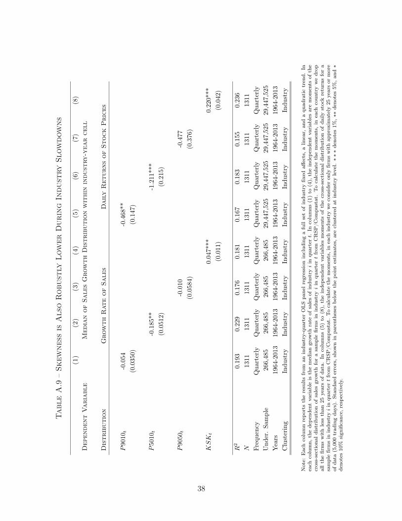
Tab

leA

.9–

Skew

ness

isA

lso

Robu

stly

Low

erD

urin

gIn

dus

try

Slow

dow

ns

(1)

(2)

(3)

(4)

(5)

(6)

(7)

(8)

Dependent

Variable

Median

of

Sales

Grow

th

Distribution

within

industry-year

cell

Distribution

Grow

th

Rate

of

Sales

Daily

Returns

of

Stock

Prices

P9010

t-0

.054

-0.4

68**

(0.0

350)

(0.1

47)

P5010

t-0

.185

**-1

.211

***

(0.0

512)

(0.2

15)

P9050

t-0

.010

-0.4

77(0

.058

4)(0

.376

)

KSK

t0.

047*

**0.

220*

**(0

.011

)(0

.042

)

R2

0.19

30.

229

0.17

60.

181

0.16

70.

183

0.15

50.

236

N13

1113

1113

1113

1113

1113

1113

1113

11Fr

eque

ncy

Qua

rter

lyQ

uart

erly

Qua

rter

lyQ

uart

erly

Qua

rter

lyQ

uart

erly

Qua

rter

lyQ

uart

erly

Und

er.

Sam

ple

266,

485

266,

485

266,

485

266,

485

29,4

47,5

2529

,447

,525

29,4

47,5

2529

,447

,525

Yea

rs19

64-2

013

1964

-201

319

64-2

013

1964

-201

319

64-2

013

1964

-201

319

64-2

013

1964

-201

3C

lust

erin

gIn

dust

ryIn

dust

ryIn

dust

ryIn

dust

ryIn

dust

ryIn

dust

ryIn

dust

ryIn

dust

ry

Not

e:E

ach

colu

mn

repo

rts

the

resu

lts

from

anin

dust

ry-q

uart

erO

LS

pane

lre

gres

sion

incl

udin

ga

full

set

ofin

dust

ryfix

edaff

ects

,a

linea

r,an

da

quad

rati

ctr

end.

Inea

chco

lum

n,th

ede

pend

ent

vari

able

isth

em

edia

ngr

owth

rate

ofsa

les

ofin

dust

ryi

inqu

arte

rt.

Inco

lum

ns(1

)to

(4),

the

inde

pend

ent

vari

able

sar

em

omen

tsof

the

cros

s-se

ctio

naldi

stri

buti

onof

sale

sgr

owth

for

asa

mpl

efir

ms

inin

dust

ryi

inqu

arte

rt

from

CR

SP/C

ompu

stat

.To

calc

ulat

eth

em

omen

ts,in

each

coun

try

we

drop

allth

efir

ms

wit

hle

ssth

an25

year

sof

data

.In

colu

mns

(5)

to(8

),th

ein

depe

nden

tva

riab

les

mom

ents

ofth

ecr

oss-

sect

iona

ldi

stri

buti

onof

daily

stoc

kre

turn

sfo

ra

sam

ple

firm

sin

indu

stry

iin

quar

tertfr

omC

RSP

/Com

pust

at.

To

calc

ulat

eth

em

omen

ts,i

nea

chin

dust

ryw

eco

nsid

eron

lyfir

ms

wit

hap

prox

imat

ely

25ye

ars

orm

ore

ofda

ta(5

,000

trad

ing

days

).St

anda

rder

rors

,sho

wn

inpa

rent

hese

sbe

low

the

poin

tes

tim

ates

,are

clus

tere

dat

indu

stry

leve

l.⇤⇤⇤

deno

tes

1%,⇤

⇤de

note

s5%

,and

⇤de

note

s10

%si

gnifi

canc

e,re

spec

tive

ly.

38

Tab

leA

.10

–Sk

ewne

ssis

Robu

stly

Pro

cycl

ical

for

Seve

ral

Fir

m-L

evel

Out

com

es

(1)

(2)

(3)

(4)

Dep

enden

tVar

iabl

eG

row

thR

ate

of

GD

P

Dis

trib

utio

nSa

les

Gro

wth

Pro

fits

Gro

wth

Inve

ntori

esG

row

thEm

ploy

men

tG

row

th

KSK

t0.

078*

**0.

039*

**0.

044*

*0.

095*

**(0

.013

)(0

.015

)(0

.022

)(0

.020

)

N20

019

312

050

Freq

uenc

yQ

uart

erly

Qua

rter

lyQ

uart

erly

Ann

ual

Und

er.

Sam

ple

266,

485

266,

485

266,

485

266,

485

Year

s19

64-2

013

1964

-201

319

80-2

013

1964

-201

3

Not

e:E

ach

colu

mn

repo

rts

adi

ffere

ntti

me

seri

esO

LS

regr

essi

onin

clud

ing

aco

nsta

ntan

da

linea

rtr

end.

Inea

chco

lum

n,th

ede

pend

ent

vari

able

isth

egr

owth

rate

ofG

DP

per

capi

tabe

twee

nqu

arte

rt

and

the

sam

equ

arte

rof

the

follo

win

gye

ar.

The

inde

pend

ent

vari

able

sar

em

omen

tsof

the

cros

s-se

ctio

nald

istr

ibut

ion

ofth

egr

owth

rate

ofre

alqu

arte

rly

sale

s(c

olum

n(1

)),

real

quar

terl

ypr

ofits

(col

umn

(2))

,re

alva

lue

ofqu

arte

rly

inve

ntor

ies

(col

umn

(3))

,an

dan

nual

grow

thra

teof

empl

oym

ent

(col

umn

(4))

ofa

sam

ple

ofC

ompu

stat

firm

sw

ith

mor

eth

an25

year

sof

data

(100

quar

ters

).In

vent

ory

data

star

tsin

1971

,bu

tth

esa

mpl

eis

very

smal

lto

have

am

eani

ngfu

lm

easu

reof

skew

ness

.E

mpl

oym

ent

ison

lyav

aila

ble

atan

annu

alfr

eque

ncy

soth

ere

gres

sion

,us

esan

nual

GD

Pgr

owth

.N

ewey

–Wes

tst

anda

rder

rors

are

appl

ied

inea

chco

lum

nto

cont

rolf

orau

toco

rrel

atio

n(m

axof

1la

g).⇤⇤⇤

deno

tes

1%,⇤

⇤de

note

s5%

,and

⇤de

note

s10

%si

gnifi

canc

e,re

spec

tive

ly.

39

Figure A.7 – Skewness is Procyclical for different firm-size groups

−3−2

−10

1

Skew

ness

: Kel

ly(n

orm

aliz

ed to

mea

n 0,

SD

1)

1 2 3 4 5 6 7 8 9 10GDP growth deciles

Skewness of the Quarterly Sales Growth

Small Medium Medium/Large Large

−2−1

01

2

Skew

ness

: Kel

ly(n

orm

aliz

ed to

mea

n 0,

SD

1)

1 2 3 4 5 6 7 8 9 10GDP growth deciles

Skewness of the Daily Stock Returns

Small Medium Medium/Large Large

Note: The figure is based on quarterly sales data and daily stock returns data for the United States over the period 1970to 2014. Each quarter is placed into a bin based on the decile of the annual growth rate of quarterly GDP, with binsfrom 1 to 10, where 1 is the lowest decile growth and 10 is the highest. Size classes are constant within a year and aredefined by the quartiles of the industry-specific distribution of average employment defined by the average employmentbetween period t � 1 and t � 3. Industries are defined as in Figures A.5 and A.6. Both the cross-sectional moments andthe industry-specific size distribution are calculated over a sample of publicly traded firms from the CRSP/Compustatdata set with 10 or more years of data (40 quarters in the case of sales data and 2000 trading days in the case of stockprices).

40

Tab

leA

.11

–Sk

ewne

ssis

Robu

stly

Low

erD

urin

gSl

owdow

nsW

ithi

nFir

m-S

ize

Gro

ups

(1)

(2)

(3)

(4)

(5)

(6)

(7)

(8)

Dependent

Variable

Median

of

the

Sales

Grow

th

Distribution

within

the

size

class-quarter

cell

Distribution

Sales

Grow

th

Within

Size

Class-Q

uarter

Cell

Daily

Stock

Returns

Within

Size

Class-Q

uarter

Cell

P9010

t-0

.234

***

-0.9

16**

*(0

.019

)(0

.087

)

P5010

t-0

.392

***

-1.5

27**

*(0

.034

)(0

.171

)

P9050

t-0

.023

***

-1.8

98**

*(0

.003

)(0

.162

)

KSK

t0.

158*

**0.

113*

**(0

.008

)(0

.003

)

R2

694

694

694

694

694

694

694

694

N0.

277

0.39

60.

0912

0.39

60.

197

0.16

50.

219

0.12

7Fr

eque

ncy

Qua

rter

lyQ

uart

erly

Qua

rter

lyQ

uart

erly

Qua

rter

lyQ

uart

erly

Qua

rter

lyQ

uart

erly

Und

er.

Sam

ple

511,

122

511,

122

511,

122

511,

122

41,6

43,4

6641

,643

,466

41,6

43,4

6641

,643

,466

Yea

rs19

70-2

013

1970

-201

319

70-2

013

1970

-201

319

70-2

013

1970

-201

319

70-2

013

1970

-201

3C

lust

erin

gSi

zeC

lass

Size

Cla

ssSi

zeC

lass

Size

Cla

ssSi

zeC

lass

Size

Cla

ssSi

zeC

lass

Size

Cla

ss

Not

e:E

ach

colu

mn

repo

rts

the

resu

lts

from

asi

zecl

ass-

quar

ter

OLS

pane

lre

gres

sion

incl

udin

ga

full

set

ofsi

ze-c

lass

fixed

effec

ts,a

linea

r,an

da

quad

rati

ctr

end.

Inea

chco

lum

n,th

ede

pend

ent

vari

able

isth

em

edia

ngr

owth

rate

ofsa

les

ofsi

ze-c

lass

iin

quar

tert.

Inco

lum

ns(1

)to

(4),

the

inde

pend

ent

vari

able

sar

em

omen

tsof

the

cros

s-se

ctio

nald

istr

ibut

ion

ofsa

les

grow

thfo

ra

sam

ple

firm

sin

the

size

-cla

ssiin

quar

tertfr

omC

RSP

/Com

pust

at.

Inco

lum

ns(5

)to

(8),

the

inde

pend

ent

vari

able

sar

em

omen

tsof

the

cros

s-se

ctio

naldi

stri

buti

onof

daily

stoc

kre

turn

sof

asa

mpl

efir

ms

inin

dust

ryi

inqu

arte

rt

from

CR

SP/C

ompu

stat

.Si

zecl

asse

sar

eco

nsta

ntw

ithi

na

year

and

are

defin

edby

the

quar

tile

sof

the

indu

stry

-spe

cific

dist

ribu

tion

ofav

erag

eem

ploy

men

tde

fined

byth

eav

erag

eem

ploy

men

tbe

twee

npe

riod

t�

1an

dt�

3.

Indu

stri

esar

ede

fined

asin

Fig

ures

A.5

and

A.6

.B

oth

the

cros

s-se

ctio

nalm

omen

tsan

dth

ein

dust

ry-s

peci

ficsi

zedi

stri

buti

onar

eca

lcul

ated

over

asa

mpl

eof

publ

icly

trad

edfir

ms

from

the

CR

SP/C

ompu

stat

data

set

wit

h10

orm

ore

year

sof

data

(40

quar

ters

inth

eca

seof

sale

sda

taan

d20

00tr

adin

gda

ysin

the

case

ofst

ock

pric

es).

Stan

dard

erro

rs,s

how

nin

pare

nthe

ses

belo

wth

epo

int

esti

mat

es,a

recl

uste

red

atth

esi

ze-c

lass

leve

l.⇤⇤⇤

deno

tes

1%,⇤

⇤de

note

s5%

,and

⇤de

note

s10

%si

gnifi

canc

e,re

spec

tive

ly.

41

Figure A.8 – Skewness is Procyclical Within Different Groups of Coun-tries

−3−2

−10

12

Skew

ness

: Kel

ly(n

orm

aliz

ed to

mea

n 0,

SD

1)

1 2 3 4 5 6 7 8 9 10GDP growth deciles

Developing Countries

Sales Growth Stock ReturnsGDP Growth Index Returns

−3−2

−10

12

Skew

ness

: Kel

ly(n

orm

aliz

ed to

mea

n 0,

SD

1)

1 2 3 4 5 6 7 8 9 10GDP growth deciles

Developed Countries

Sales Growth Stock ReturnsGDP Growth Index Returns

Note: Each panel of Figure A.8 is based on annual, quarterly, and daily data for a sample of developed and developingcountries over the period 1986 to 2014. Developing countries are those in the upper half of the distribution of GDP percapita in the year 2000 (i.e. Germany, United States, etc.) while developing countries are those in the lower half of thedistribution (i.e. Argentina, Chile, etc.).

42

Figure A.9 – Dispersion is CounterCyclical Within Groups of Countries

−10

12

3

Dis

pers

ion:

P90

− P

10(n

orm

aliz

ed to

mea

n 0,

SD

1)

1 2 3 4 5 6 7 8 9 10GDP growth deciles

Developing CountriesSales Growth Stock ReturnsGDP Growth Index Returns

−2−1

01

2

Dis

pers

ion:

P90

− P

10(n

orm

aliz

ed to

mea

n 0,

SD

1)

1 2 3 4 5 6 7 8 9 10GDP growth deciles

Developed Countries

Sales Growth Stock ReturnsGDP Growth Index Returns

Note: Each panel of Figure A.9 is based on annual, quarterly, and daily data for a sample of developed and developingcountries over the period 1986 to 2014. Developing countries are those in the upper half of the distribution of GDP percapita in the year 2000 (i.e. Germany, United States, etc.) while developing countries are those in the lower half of thedistribution (i.e. Argentina, Chile, etc.).

43

Table A.12 – Moments of Sales Growth Distribution with Entry and Exit

(1) (2) (3) (4)Dependent Variable Growth rate of GDP

Distribution Sales Growth

P9010t 0.001(0.005)

P5010t –0.158***(0.034)

P9050t 0.004(0.005)

KSKt 0.031***(0.010)

N 200 200 200 200Frequency Quarterly Quarterly Quarterly QuarterlyUnder. Sample 266,485 266,485 266,485 266,485Years 1964-2013 1964-2013 1964-2013 1964-2013

Note: Each column reports a different time series OLS regression including a constant and a linear trend (robust standarderrors in parentheses below the point estimates). In each column, the dependent variable is the growth rate of the GDPper capita between quarter t and the same quarter of the following year. The independent variables are moments of thecross-sectional distribution of the arc percentage growth rate of quarterly sales for a sample of Compustat firms with 10years or more of data (40 quarters). Newey-West standard errors are applied in each column to control for auto correlation(max of 1 lag). ⇤ ⇤ ⇤ denotes 1%, ⇤⇤ denotes 5%, and ⇤ denotes 10% significance, respectively.

44