Embed Size (px)
Citation preview

53
American Economic Journal: Macroeconomics 2 (October 2010): 53–87http://www.aeaweb.org/articles.php?doi=10.1257/mac.2.4.53
Macroeconomists need reliable empirical estimates of the extent to which household consumption is insulated from income fluctuations for at least
two reasons. First, imperfect risk sharing is at the heart of heterogeneous-agents, incomplete-markets models. Thus, the availability of a simple empirical measure of consumption insurance would allow researchers to compare, parsimoniously, the predictions of different incomplete-markets models along their most salient dimen-sion. Second, macroeconomic models are routinely used for policy evaluation and design. For example, a reform from a progressive to a flat tax system is judged on the basis of the gains from reduced distortions and the losses from lower redistribution. But the size of the latter margin depends on how much smoothing agents can do on their own, through private risk sharing. Getting this magnitude right in the model is a key requisite if the model is to deliver reliable predictions for policy experiments.
Today, the measurement of consumption insurance against earnings shocks acquires particular salience in the US economy because of the recent sharp increase in cross-sectional wage dispersion. Understanding the macroeconomic and welfare implications of this dramatic change in the wage structure requires models with the correct degree of risk-sharing.1
1 Dirk Krueger and Fabrizio Perri (2006); Jonathan Heathcote, Kjetil Storesletten, and Violante (2008b); and Fatih Guvenen and Burhanettin Kuruscu (2009) offer alternative views in this debate.
* Kaplan: Federal Reserve Bank of Minneapolis, 90 Hennepin Avenue, Minneapolis, MN 55401, and University of Pennsylvania (e-mail: [email protected]); Violante: New York University, 19 West Fourth Street, New York, NY 10013, Centre for Economic Policy Research, Institute for Fiscal Studies (IFS), and National Bureau of Economic Research (e-mail: [email protected]). We thank Richard Blundell, Eric French, Luigi Pistaferri and three anonymous ref-erees for useful suggestions. Violante is grateful to the National Science Foundation (grant SES-0418029) for financial support. The views expressed here are those of the authors and not necessarily those of the Federal Reserve Bank of Minneapolis or the Federal Reserve System. Previous versions of the paper circulated with the title “How Much Insurance in Bewley Models?”
† To comment on this article in the online discussion forum, or to view additional materials, visit the articles page at http://www.aeaweb.org/articles.php?doi=10.1257/mac.2.4.53.
How Much Consumption Insurance Beyond Self-Insurance?†
By Greg Kaplan and Giovanni L. Violante*
We assess the degree of consumption smoothing implicit in a cali-brated life-cycle version of the standard incomplete-markets model, and we compare it to the empirical estimates of Richard Blundell, Luigi Pistaferri, and Ian Preston (2008) (BPP hereafter) on US data. Households in the data have access to more consumption insurance against permanent earnings shocks than in the model. BPP estimate that 36 percent of permanent shocks are insurable, whereas the model’s counterpart of the BPP estimator varies between 7 percent and 22 percent, depending on the tightness of debt limits. We also show that the BPP estimator has a downward bias that grows as bor-rowing limits become tighter. (JEL D31, D91, E21).
ContentsHow Much Consumption Insurance Beyond Self-Insurance?† 53
I. A Framework for Measuring Insurance 57A. Insurance Coefficients 57B. BPP Methodology 58II. A Model to Interpret the BPP Findings 61A. The Economy 61B. Calibration 63III. Results 65A. Consumption and Wealth Over the Life Cycle 66B. BPP Insurance Coefficients in the Data and the Model 67C. Accuracy of the BPP Methodology 67D. Age Profiles of Insurance Coefficients 69E. Sensitivity Analysis 71IV. Advance Information 73A. Short-run Anticipation of Permanent Shocks 75B. Long-Run Foreknowledge of Income Paths 77V. Persistent Income Shocks 78A. Comparison with Storesletten-Telmer-Yaron 82VI. Conclusions 84REFERENCES 85

54 AMERIcAn EcOnOMIc JOURnAL: MAcROEcOnOMIcS OctOBER 2010
The empirical assessment of the transmission of income shocks into consump-tion is undermined by two difficulties. First, one needs both longitudinal data on income and on a comprehensive measure of consumption. In the United States, such a dataset is not available. As a result, authors have either opted for using Panel Study of Income Dynamics (PSID) and Consumer Expenditure Survey (CEX) data alone (Robert E. Hall and Frederic S. Mishkin 1982; Joseph G. Altonji and Aloysius Siow 1987; John H. Cochrane 1991; Barbara J. Mace 1991; Susan Dynarski and Jonathan Gruber 1997), or opted for constructing synthetic cohorts to merge high-quality cross-sectional income and consumption data (Orazio Attanasio and Steven J. Davis 1996). Second, one needs to identify individual income shocks in the data. From the shape of the empirical autocovariance function of individual income, it is well known that income changes are best described by a combination of highly persis-tent and highly transitory shocks (Thomas E. MaCurdy 1982; John M. Abowd and David Card 1989; Blundell and Preston 1998). However, in panel data, one observes only the total income change and cannot disentangle the realization of the shocks of different persistence. As a consequence, some authors have chosen to simply measure the response of consumption to total income changes (Altonji and Siow 1987; Krueger and Perri 2005, 2008), whereas others have used proxies for perma-nent and transitory income changes (e.g., disability and short unemployment spells, respectively) in an attempt to separately identify the two shocks (Cochrane 1991; Dynarski and Gruber 1997). Finally, a large literature tries to estimate the consump-tion response of households to tax rebates (Nicholas S. Souleles 1999; Matthew D. Shapiro and Joel Slemrod 2003). Often unclear is whether such tax rebates are perceived as a permanent or transitory change in income by households. Moreover, consumers’ response to the rebate depends on whether they expect a simultaneous change in government purchases.
In a recent paper, BPP make some important progress in overcoming these two difficulties. First, the authors construct a new panel dataset for the United States with household information on income and nondurable consumption.2 Next, they use this dataset to estimate consumption insurance coefficients for permanent and transitory idiosyncratic income shocks, i.e., the fraction of the shocks that does not translate into movements in consumption. We return to the details of their methodology later. They find that 36 percent of permanent shocks and 95 percent of transitory shocks to disposable (i.e., post taxes and transfers) labor income are insurable. These find-ings are qualitatively consistent with a large literature that rejects full insurance in the US economy (Cochrane 1991; Attanasio and Davis 1996; Fisher and Johnson 2006), and with the “excess smoothness” finding (i.e., consumption reacts to per-manent shocks less than what is predicted by the permanent income hypothesis) in
2 The key step is, following Jonathan Skinner (1987), the imputation of a measure for nondurable consumption for each individual/year observation in the PSID by exploiting the fact that food consumption is available in both the PSID and the CEX. From the CEX, one can estimate a relationship between food and nondurable consump-tion expenditures—a food demand function—and then invert the demand function and implement the imputa-tion procedure at the household level, based on the reported value for food consumption in the PSID records. In Jonathan D. Fisher and David S. Johnson (2006), a recent implementation of this strategy is applied to the study of consumption mobility.

VOL. 2 nO. 4 55kAPLAn And VIOLAntE: cOnSUMPtIOn InSURAncE
the context of aggregate and individual consumption (John Y Campbell and Angus Deaton 1989; Attanasio and Nicola Pavoni 2007).
In light of the previous discussion, we argue that the BPP insurance coefficients should become central in quantitative macroeconomics. They provide a yardstick to measure whether current incomplete-markets macroeconomic frameworks used for quantitative analysis admit the right amount of household insurance. In this paper, we begin this investigation within what is, arguably, the standard incomplete mar-kets (SIM) model, a world where households have no access to state-contingent claims, but can self-insure by trading a non-state-contingent bond. In the last decade, this model has become the leading tool for quantitative analysis in macroeconom-ics.3 We choose a life-cycle version of the model with capital in positive net supply where households have constant relative risk aversion (CRRA) utility, are subject to permanent and transitory shocks to earnings while they work, and during retire-ment receive social security benefits through a scheme that closely mimics the US system. Households smooth shocks by borrowing, as long as their accumulated debt is below a pre-specified limit. We consider two extreme cases: a natural borrowing limit and a zero borrowing limit. They also save for life-cycle and precautionary rea-sons, and their wealth helps to absorb income shocks. The calibration of the model uses standard parameter values in this literature.
By simulating an artificial panel from the model, we address two questions:
• How does the BPP empirical estimate for consumption smoothing compare to its SIM model counterpart? Put differently, how much consumption insur-ance is there in the data, over and beyond self-insurance?
• Does the BPP methodology yield reliable estimates of insurance coefficients?
Answering this last question is possible because in the model we can compute both the true insurance coefficient and the value for the BPP (2008)estimator.
Our findings can be summarized as follows. First, the model counterpart of the BPP insurance coefficient for transitory shocks is 94 percent in the natural borrow-ing constraint (NBC) economy and 82 percent in the zero borrowing constraint (ZBC) economy, and hence close to the empirical estimate of 95 percent. The insurance coefficient for permanent shocks is 22 percent in the NBC economy and only 7 percent in the ZBC economy. In both cases, the model contains less insur-ance with respect to permanent shocks relative to the BPP empirical estimate of 36 percent, even though this point estimate is quite imprecise. Moreover, the life-cycle pattern of insurance coefficients for permanent shocks is sharply increasing and convex, whereas BPP find no evidence of a clear age profile. This discrepancy sug-gests that the model generates too much consumption smoothing for older workers nearing retirement, but too little smoothing for workers in the early stages of their life cycle.
Second, we assess the reliability of the estimator proposed by BPP to identify insurance for each type of shock. We find that the estimator works very well for
3 See Heathcote, Storesletten, and Violante (2009) for a recent survey of this literature.

56 AMERIcAn EcOnOMIc JOURnAL: MAcROEcOnOMIcS OctOBER 2010
transitory shocks, but it tends to systematically underestimate the true coefficient for permanent shocks, which are 23 percent in both the NBC and the ZBC economies. The reason is that the estimation procedure, analogous to an instrumental variables approach, exploits an orthogonality condition between consumption growth and a particular linear combination of past and future income shocks. The bias results from the fact that this orthogonality condition holds only approximately in the model. When borrowing constraints are loose, the bias is negligible, but when they are tight, this failure becomes severe. If we correct for this bias, the empirical insur-ance coefficients could be even larger than those estimated.
In light of these two findings, we explore two alternative ways in which SIM models could generate less sensitivity of consumption to permanent shocks. We first allow agents to have some foresight about future income realizations. We model this advance information in two ways. When we let agents know a fraction of the permanent shock one period ahead of time (short-run foreknowledge), we show that the BPP estimator of insurance coefficients is, in essence, invariant to the amount of advanced information. When we assume that earnings have an individ-ual-specific deterministic trend that is known by the agent from “birth” (long-run foreknowledge), then the BPP estimator reflects a mix of insurance and foresight, and increases with the amount of advance information. However, we argue that for plausibly calibrated heterogeneity in income profiles, the estimated coefficients remain lower than in the data. Overall, advance information does not bridge the gap between model and data.
Next, we generalize the statistical process for earnings. Instead of restricting it to an I(1) as assumed by BPP, we posit that the persistent component of the income process is AR(1). We first show that the BPP method performs quite well, even under this misspecification error, for high degrees of persistence (ρ). Next, we docu-ment that for ρ between 0.93 and 0.97, depending on the tightness of the constraint, the insurance coefficient for persistent shocks in the model can, on average, achieve its empirical value. However, its life-cycle profile remains quite steep. We discuss some modifications of the model that either shift wealth holdings from the old to the young, allowing the former to self-insure more effectively, or introduce explicit insurance against labor market shocks for younger agents.
Finally, we contrast the concept of insurance coefficient as a measure of risk shar-ing with another norm for risk sharing proposed by Deaton and Christina Paxson (1994) and Storesletten, Christopher I. Telmer, and Amir Yaron (2004) and used extensively in the literature, the steepness of life-cycle consumption dispersion. There is no contradiction between our result that the model stops short of replicat-ing the empirical insurance coefficient and their finding that it generates the right increase in consumption inequality over the life cycle.
The rest of the paper is organized as follows. Section I introduces a general frame-work for measuring insurance and describes the BPP methodology as a special case. Section II outlines the version of the SIM model we use for our experiments and describes its parametrization. Section III contains the results from our benchmark economies and from a series of sensitivity analyses. Section IV introduces advance information into the model. Section V analyzes the robustness of our findings to the degree of persistence of income shocks. Section VI concludes the paper.

VOL. 2 nO. 4 57kAPLAn And VIOLAntE: cOnSUMPtIOn InSURAncE
I. A Framework for Measuring Insurance
A. Insurance coefficients
Income Process.—Suppose that residual (i.e., deviations from a deterministic and predictable experience profile common across all households) log-earnings yit for household i of age t can be represented as a linear combination of current and lagged shocks
(1) yit = ∑j=0
t
a j ′x i,t−j ,
where xi,t−j is an (m ×1) vector of shocks with generic element xit, and aj is an (m ×1) vector of coefficients. The shocks are independently and identically dis-tributed in the population and over time. Let σ = (σ1, … , σm)′ be the corresponding vector of variances for these shocks. This formulation is extremely general and incor-porates, for example, linear combinations of ARIMA processes with fixed effects.
Insurance coefficients.—Let cit be log consumption for household i at age t. We define the insurance coefficient for shock xit as
(2) ϕx = 1 − cov(Δcit, xit)_
var(xit) ,
where the variance and covariance are taken cross-sectionally over the entire popu-lation of households. One can similarly define the insurance coefficient at age t(denoted by ϕ t
x ), where variance and covariance are taken conditionally on all house-holds of age t. The insurance coefficient in (2) has an intuitive interpretation; it is the share of the variance of the x shock that does not translate into consumption growth.
Identification and Estimation.—In any given model, it is straightforward to cal-culate (2) by simulation, since the shocks are observable in the model. However, identifying and estimating (2) from the data poses a crucial difficulty. The individual shocks are not directly observed and cannot be identified from a finite panel of income data.4
Suppose panel data on households’ income and consumption are available. Let yi be the vector of income realizations for individual i at all ages t = 0, … , t, and let g t
x (yi) index measurable functions of this income history, one for each t and for each shock x. Identification and estimation of insurance coefficients for shock x can be achieved by finding functions g t
x such that
(3) var(xit) = cov(Δyit, g t x (yi)),
cov(Δcit, xit) = cov(Δcit, g t x (yi)),
4 Note that it is not sufficient to identify the variances of the different shocks, i.e., the vector σ. Rather, the realizations of the shocks must be identified, household by household. With a very long sequence of observations, realizations may be identified using filtering techniques. However the pervasive heterogeneity and the short time dimension of commonly available panel datasets are likely to make filtering techniques unreliable in this context.

58 AMERIcAn EcOnOMIc JOURnAL: MAcROEcOnOMIcS OctOBER 2010
and then constructing ϕ x as
(4) ϕx = 1 − cov(Δcit, g t
x (yi))__cov(Δyit, g t
x (yi)).
Verifying the first condition in (3) only requires knowledge of the true income pro-cess, but verifying the second condition also requires knowledge of how the empiri-cal consumption allocation depends on the entire income vector (past and future realizations of the shocks). Thus, it requires knowing the true data-generating pro-cess (i.e., the model) for consumption.
This approach is best thought of in terms of instrumental variables regressions. If g t
x (yi) satisfies the conditions in (3), then the resulting expression for 1 − ϕx is equivalent to the coefficient from an instrumental variables regression of consump-tion changes on income changes, using g t
x (yi) as an instrument. In general, the cor-rect choice of instrument depends on the particular specification of the income process, and the underlying true model for consumption. To progress further, one has to make assumptions about both.
B. BPP Methodology
One can view the BPP methodology precisely as a choice of a particular income process and consumption allocation.
BPP (2008)Income Process.—BPP choose the sum of a random walk (perma-nent) and an MA(1) component as their income process. In what follows, to avoid keeping track of an extra state variable in the model’s computation, we simplify the latter component to an independently and identically distributed shock.5 This choice corresponds to setting m = 2, xit = (ηit, εit)′, a0 = (1, 1)′, and aj= (1, 0)′ for j ≥1 in (1), which yields
(5) yit = zit + εit ,
where zit follows a unit root process with shock ηit, and εit is an independently and identically distributed income shock with variances ση and σε, respectively.6 It fol-lows that income growth can be written as
(6) Δyit = ηit + Δεit .
5 This simplification means that our transitory component is slightly more short-lived compared to the BPP component. One should keep this in mind when comparing the insurance coefficients for transitory shocks obtained by simulating the model with the BPP counterpart. We conjecture this effect is quantitatively minor. Moreover, it has no bearing on the analysis of permanent shocks, which is the main focus of our study.
6 BPP (2008)allow the variances of the shocks to be time-varying in their estimation. Once again, we chose an income process with constant variances of the shocks to keep the computation of the model manageable. In Section III, we show that our results are robust to plausible changes in the magnitude of permanent and transitory volatility, so this simplification is innocuous.
VOL. 2 nO. 4 59kAPLAn And VIOLAntE: cOnSUMPtIOn InSURAncE
This is a very common income process in the empirical labor literature, at least since MaCurdy (1982) and Abowd and Card (1989), who showed that this specification is parsimonious and yet fits income data well. In Section V, we verify the robustness of our results to more general specifications of the income process.
BPP consumption Model.—BPP assume that the following pair of orthogonality conditions hold for the true consumption allocation:
(NF) cov(Δcit, ηi, t +1) = cov(Δcit, εi,t +1) = 0,
(SM) cov(Δcit, ηi,t−1) = cov(Δcit, εi,t −2) = 0.
The first assumption means that the agent has “No Foresight” (or no advanced infor-mation) about future shocks. The second assumption translates into “Short Memory” (or short history dependence) of the consumption allocation with respect to shocks.7
Under these assumptions, BPP propose a strategy to identify and estimate the insurance coefficients. For the transitory shock ε, they set g t
ε (yi) = Δyi, t +1 and note that
(7) cov(Δyit , Δyi, t +1) = −var(εit),
cov(Δcit, Δyi, t +1) = −cov(Δcit, εit),
whereas for the permanent shocks η, they set g t η (yi) = Δyi, t −1 + Δyit + Δyi, t +1 and
note that
(8) cov(Δyit, Δyi, t −1 + Δyit + Δyi, t +1) = var(ηit),
cov(Δcit, Δyi, t −1 + Δyit + Δyi, t +1) = cov(Δcit, ηit).
Combining (4) with (7) and (8) confirms that these instruments do correctly iden-tify the insurance coefficients (ϕη, ϕε). It is easy to verify that only the orthogonality condition in (NF) is required for the identification of the insurance coefficients for transitory shocks, whereas both (NF) and (SM) are needed for permanent shocks.
In what follows, we call ϕ BPP x the insurance coefficient estimator based on the
BPP methodology. When the orthogonality conditions hold, ϕ BPP x = ϕx, but when
they do not there will be a bias in ϕ BPP x .8
7 To be precise, BPP start off their analysis from the consumption growth allocation Δcit
= πit η ηit + π it ε εit + ξit,
where πit η and π it ε are the marginal propensity to consume out of permanent and transitory shocks, and ξit is a resid-
ual component. The choice of this specification is motivated by the fact that, according to BPP, it approximates well the solution of a life cycle optimization problem where agents have CRRA utility. The assumption implicit in the BPP study is that (πit η , π it
ε , ξit) are all independent of income innovations at every relevant lead and lag.8 In their estimation, BPP make use of the entire variance-covariance matrix of (Δcit, Δyit). However, even
with this more complex estimation procedure, identification crucially hinges upon the (NF) and (SM) assump-tions stated earlier.

60 AMERIcAn EcOnOMIc JOURnAL: MAcROEcOnOMIcS OctOBER 2010
Generality of the BPP Approach.—The obvious question, at this point, is: how general are assumptions (NF) and (SM)? In the absence of advance information about future earnings realizations, (NF) holds. But, in certain instances, it fails. An example is in the presence of individual-specific predictable age-earnings profiles, a common class of income processes in the empirical labor literature introduced by Lee A. Lillard and Yoram Weiss (1979). We return to this point in Section IV.
With respect to assumption (SM), one can verify whether it holds in general only in models where the consumption allocation has a closed form. In the absence of a closed form, as in the standard incomplete-markets economy that we study in this paper, one must rely on model simulations.
The consumption literature offers few closed-form solutions. It is easy to see that complete-markets and autarkic economies satisfy (SM). Under complete markets, idiosyncratic shocks do not affect consumption, hence cov(Δcit, xit) = 0 and ϕx = 1. In autarky, Δcit = Δyit, hence, cov(Δcit, xit) = var(xit) and ϕx = 0. Note that in these two extreme cases, the value of ϕx is independent of the durability of the shock.
The strict version of the life-cycle, rational expectations, permanent income hypothesis (PIH), where agents have quadratic utility, live for t periods, and can borrow and save at a constant risk-free rate r equal to the discount rate, generates the following rule for changes in consumption, when combined with the income process in (5) specified in levels
Δcit = ηit + χtεit ,
where χt= (r/(1 + r))(1/(1 − (1 + r)−(t−t+1))).9 Hence, the PIH satisfies the BPP assumptions, and the insurance coefficients (defined in terms of levels rather than logs) for a PIH economy are ϕ t
η = 0 and ϕ t ε = 1 − χt . These values imply full
transmission of permanent shocks to consumption and a smoothing coefficient for transitory shocks that starts near one and decreases monotonically toward zero as the end of life becomes nearer. In what follows, we call this latter result the “horizon effect.”10
Finally, one can verify that the BPP assumptions hold in the partial insurance economy developed by Heathcote, Storesletten, and Violante (2007) and in the moral-hazard economy studied by Attanasio and Pavoni (2007), both of which pro-vide closed-form solutions.
These examples demonstrate that, in a wide variety of economic environments, it is possible to justify consumption allocations that are consistent with (NF) and (SM) and the BPP estimator is unbiased. But is this true also for standard incomplete-markets models? We answer this question in detail in the next sections.
9 We use upper case letters to denote variables in levels and lower case letters to denote variables in logs.10 In the context of the PIH, this structural identification approach based on closed forms has a long history.
Pioneering work by Thomas J. Sargent (1978) on aggregate data, and Hall and Mishkin (1982) on longitudinal PSID data, exploits restrictions across income and consumption processes implied by the PIH to estimate the model’s parameters. A more recent example is Blundell and Preston (1998).
VOL. 2 nO. 4 61kAPLAn And VIOLAntE: cOnSUMPtIOn InSURAncE
BPP Findings.—Straightforward application of a minimum distance algorithm allows estimation of the cross-sectional covariances in (7) and (8).11 BPP reach three main findings. First, when labor income is defined as household earnings after tax and transfers, the insurance coefficient for permanent shocks ϕ BPP η
is estimated to be 0.36 (standard error 0.09). Second, the insurance coefficient for transitory shocks ϕ BPP ε is estimated to be 0.95 (standard error 0.04). Third, BPP find no clear evidence of a significant age profile in the insurance coefficients for permanent shocks.12 In order to assess the robustness of this result, we split BPP’s sample into two groups based on age, and repeated their empirical procedure. We found that for the younger half of the sample (30–47 years old) the insurance coefficient is 0.43 (standard error 0.12), whereas for the older group (48–65 years old) the insurance coefficient is 0.19 (standard error 0.19). The large standard errors that arise from reducing the sample size by half mean that one cannot reject a null hypothesis that the coeffi-cients for the two groups are equal. We conclude that there is no strong evidence to support a significant age profile in ϕ BPP η
.
II. A Model to Interpret the BPP Findings
In this section, we outline and calibrate a life-cycle SIM economy (Deaton 1991; R. Glenn Hubbard, Jonathan Skinner, and Stephen P. Zeldes 1995; Ayse Imrohoroglu, Selahattin Imrohoroglu, and Douglas H. Joines 1995; José-Víctor Ríos-Rull 1995; Mark Huggett 1996; Christopher D. Carroll 1997). We then simu-late an artificial panel of household income and consumption from the model, and calculate the model’s counterpart of the BPP insurance coefficients. By comparing them to the empirical values estimated by BPP,we can learn whether the observed amount of consumption insurance can be replicated in an environment where agents self-insure by borrowing and saving through a risk-free asset.
Moreover, since, in the model, we can compute both the true insurance coef-ficients and those based on the BPP instruments, we are also in a position to assess the reliability of the BPP methodology. We will find out if and when assumptions (NF) and (SM) are violated.
A. the Economy
There is no aggregate uncertainty. The economy is populated with a continuum of households, indexed by i. Agents work until age t ret, at which time they enter into retirement. The unconditional probability of surviving to age t is denoted by ξt. We assume that ξt = 1 for the first t ret − 1 periods, so that there is no chance of dying before retirement. After retirement, ξt < 1 and all agents die by age t with cer-tainty. Altruism is assumed away. In order to focus solely on income uncertainty, we
11 Note that the model can only be estimated from panel data with at least four consecutive observations on both household income and consumption. None of the currently available US surveys have this feature. As dis-cussed in the introduction, BPP cleverly merge the CEX and PSID and construct a long panel with nondurable consumption and income observations. See BPP (2004, 2008) for details.
12 They allow for a linear age trend in ϕ BPP η and estimate a small, positive slope that is not significantly dif-
ferent from zero.
62 AMERIcAn EcOnOMIc JOURnAL: MAcROEcOnOMIcS OctOBER 2010
assume that there exist perfect annuity markets so that households are completely insured against survival risk.
Households have time-separable expected utility given by
E 0∑t=1
t
β t−1ξt u(cit).
During the working years, households receive labor income Yit which comprises three components in logs
log Yit = κt + yit
yit = zit + εit ,
where κt is a deterministic experience profile that is common across all households, and yit is the stochastic portion of income; zit is a permanent component; and εit is a transitory component. The component zit follows a random walk
zit = zi,t−1 + ηit,
where zi0 is drawn from an initial Normal distribution with mean zero and variance σ z 0 . The shocks εit and ηit have mean zero, are normally distributed with variances σε and ση, are orthogonal to each other, and are independent over time and across households in the economy. This is precisely the BPP income process.
The concept of labor income that we adopt in the model for Yit is households’ earnings after taxes and transfers, the same used by BPP in the calculation of the insurance coefficients. However, it is useful to also define gross (or pre-government) labor income as
Y it, with
Y it = G(Yit). For now, it suffices to think of the G function
as the inverse of a tax function. In the calibration section, we explain in detail how we obtain G.
Retired households receive after-tax social security transfers P(
Y i) from the government, which are a function of the entire individual vector of gross earnings realizations ˜
Y i = {
Y i1, … ,
Y it, … ,
Y i, t ret −1 }.
Households can trade a risk-free, one-period bond which pays a constant after-tax rate of return, 1 + r. We denote by Ai,t +1 the amount of this asset carried over by individual i from time t to t + 1. As usual in these models, this asset has the twin role of a store of value and of a vehicle of self-insurance. Households begin their life with initial wealth Ai0 drawn from the distribution H(Ai0) and face a lower bound A ≤0 on their asset position.
The household’s budget constraint in this economy is, therefore,
(9) cit + Ai,t +1 = (1 + r)Ait + Yit , if t < t ret
cit + aξt _ξt +1 bAi,t +1 = (1 + r)Ait + P(
Y i), if t ≥ t ret.

VOL. 2 nO. 4 63kAPLAn And VIOLAntE: cOnSUMPtIOn InSURAncE
Finally, it is useful to note that in the version of the model with A = 0, house-holds behave close to the buffer-stock, no-debt consumers characterized by Carroll (1997)—the only difference being the retirement period and the social security system.
For reasons we explain in the next section, in solving the model we do not impose restrictions that would correspond to a closed-economy general equilibrium of a production economy. However, our allocations of the baseline economy can also be interpreted as equilibrium outcomes.13
B. calibration
We calibrate the model parameters to reproduce certain key features of the US economy. Our parametrization is standard for this class of economies.
demographics.—The model period is one year. Households enter the labor mar-ket at age 25. We set t ret = 35 and t = 70. Thus, workers retire at age 60 and die with certainty at age 95. The survival rates ξt are obtained from the National Center for Health Statistics (1992).
Preferences.—We choose a CRRA specification for u(cit) with risk aversion parameter γ = 2. We explore the sensitivity of our results to values of γ in the range [1, 15].
discount Factor and Interest Rate.—The size of the stock of accumulated assets directly affects the extent to which income shocks are smoothed. Hence, it is impor-tant to ensure that the wealth to income ratio in the model is similar to that in the US economy. We set β to match an aggregate wealth-income ratio of 2.5. This is, approximately, the average wealth to average income ratio computed from the 1989 and 1992 Survey of Consumers Finances (SCF), when wealth is defined as total net worth, income is pre-tax labor earnings plus capital income, and the top 5 percent of households in the wealth distribution are excluded.14 The reason for this exclusion is comparability with the PSID and the CEX, the key sources of the BPPestimates. It is well known that both the PSID and the CEX severely undersample the top of the wealth distribution.15 We choose 1989 and 1992 as benchmark years for consistency with the sample period used by BPP. We study the sensitivity of our finding to the choice of the capital-income ratio target.
13 In particular, any chosen value for the interest rate can be rationalized as the equilibrium marginal product of capital with the appropriate value of the technology parameters (depreciation and capital share). The govern-ment budget constraint can be thought of as holding exactly by assuming that the residual between tax revenues and pension benefits represents nonvalued government consumption, and aggregate initial transfers to newborn agents distributed based on the function H (Ai0).
14 Later, we explain how, in the model, we translate after-tax income Yit into a measure of pre-tax, or gross, income
Y it that is needed to calibrate the wealth-income ratio and to determine social security benefits paid to
each household.15 Edward N. Wolff (1999,table 6) documents that the PSID and the SCF agree upon the amount of wealth
held by the median household, and by the bottom four quintiles, but large discrepancies are found at the top. As a result, in 1992 average wealth in the SCF is 50 percent higher than in the PSID, which is precisely the share of net worth held by the top 5 percent in the SCF.
64 AMERIcAn EcOnOMIc JOURnAL: MAcROEcOnOMIcS OctOBER 2010
Since our benchmark model is calibrated to generate only half of the total wealth in the US economy, we do not determine the interest rate in equilibrium. Instead, we set r = 3 percent and report results for different values of r in our robustness analysis.
Income Process.—We calibrate the common deterministic age profile for log income κt using PSID data.16 For the stochastic components of the income process, three parameters are required. These are the variance of the two shocks, σε and ση, and the cross-sectional variance of the initial value of the permanent component σ z 0 . In our benchmark calibration, we set the variance of permanent shocks to be 0.01 to match the rise in earnings dispersion over the life cycle in the PSID from age 25 to age 60. The initial variance of the permanent shocks is set at 0.15 to match the dispersion of household earnings at age 25. We set the variance of transitory shocks to be 0.05, at the BPP (2008)point estimate. We also report results from various sensitivity analyses on these values.17
Initial Wealth.—In the benchmark calibration, we assume that all households start their economic life with zero wealth, i.e., Ai0= 0. We also consider an environment in which initial wealth levels are drawn from a distribution calibrated to replicate the empirical distribution of wealth for young households in the data.18
Borrowing Limit.—We consider two alternative borrowing limits.19 We allow for borrowing subject only to the restriction that with probability one, households who live up to age t do not die in debt (i.e., the “natural debt limit”). This assump-tion represents an upper bound on the amount agents can borrow.20 We also study the self-insurance possibilities of agents when the other extreme of no borrowing, A = 0, is imposed.21
Social Security Benefits.—Social security benefits are a function of lifetime average individual gross earnings
Y i SS =(1/(t ret−1))∑t=1
t ret −1
Y it . This function is designed to mimic the actual US system. This is achieved by specifying that ben-efits are equal to 90 percent of average past earnings up to a given bend point, 32
16 The estimated profile peaks after 21 years of labor market experience at roughly twice the initial value, and then it slowly declines to about 80 percent of the peak value.
17 In particular, we run a set of simulations with ση =0.02, which is the BPP estimate for the variance of the permanent component. Such value implies an excessive rise of earnings dispersion over the life cycle. Nevertheless, it is the point estimate that is typically obtained when the permanent-transitory income process is estimated using moments in first-differences, as in BPP.
18 Precisely, we target the empirical distribution of financial wealth-earnings ratios in the population of house-holds aged 20–30 in the SCF. We assume that the initial draw of earnings is independent of the initial draw of this ratio, since in the data the empirical correlation is 0.02.
19 The model displays precautionary saving both because of prudence as defined by Miles S. Kimball (1990) and because households save to avoid hitting the debt limit (Huggett 1993).
20 The level of the natural debt limit depends on the discretization of the income process, through the level of the lowest possible income realization. In the benchmark economy, the natural borrowing limit decreases from approximately 5.8 times average annual earnings at age 25 to 2.5 times average earnings at age 50.
21 In a typical simulation of our economy with A =0, about 7 percent of households are at the constraint. These are primarily very young households. The fraction constrained decreases from 44 percent at age 26 to almost zero around age 45, but it rises again during retirement, since the optimal consumption path is downward sloping (at rate βR) and the pension income path is constant.

VOL. 2 nO. 4 65kAPLAn And VIOLAntE: cOnSUMPtIOn InSURAncE
percent from this first bend point to a second bend point, and 15 percent beyond that. The two bend points are set at, respectively, 0.18 and 1.10 times cross-sectional average gross earnings, based on the US legislation and individual earnings data for 1990. Benefits are then scaled proportionately so that a worker earning average labor income each year is entitled to a replacement rate of 45 percent (Olivia S. Mitchell and John W. R. Phillips 2006).
To compute social security benefits for each household, we need to translate net earnings Yit, our primitive earnings concept entering the working households’ budget constraint, into gross earnings
Y it. We do it by inverting the nonlinear tax function
estimated by Miguel Gouveia and Robert P. Strauss (1994)and used, for example, by Ana Castaneda, Javier Diaz-Gimenez, and Ríos-Rull (2003). The explicit func-tional form is given by
(10) τ(
Y it) = τ b S
Y it − A
Y it − τ ρ + τs B − 1 _
τ ρ T.
The values for τ b and τρ are taken from Gouveia and Strauss (1994) and set atτ b = 0.258 and τ ρ= 0.768, their estimates for 1989, the latest year available.22 The value for τs is then chosen so that the ratio of total personal current tax receipts on labor income (not including social security contributions) to total labor income is the same as for the US economy in 1990, i.e., roughly 25 percent. Given a realiza-tion for after-tax earnings Yit, we compute the corresponding gross earnings
Y it as
the solution to the equation
Y it − τ(
Y it) = Yit, which, implicitly, determines the G function defined earlier.
As in the US system, in the model the government taxes 85 percent of benefits through the function τ(·), hence, P(
Y i) in the retiree’s budget constraint (9) repre-
sents net benefits.
III. Results
All our results are based on simulating, from the invariant distribution of the model economy, an artificial panel of 50,000 households for 70 periods, a full life cycle. We have verified that increasing the sample size further does not lead to any change in the results.23 Our two benchmark economies are calibrated as described in Section IIB, and differ only through the borrowing constraint (and therefore the discount factor). The first economy has the loosest possible debt limit, the second has the tightest (zero). We refer to these two models as the NBC and the ZBC economies.
22 We exclude social security tax from the Gouveia-Strauss tax function because it is not subtracted from the net earnings definition of BPP.
23 The model is solved using the method of endogenous grid points developed by Carroll (2006) with 100 exponentially spaced grid points for assets. The grid for lifetime average earnings has 19 points. The decision rule is constrained to be linear between grid points. The permanent component is approximated using a discrete Markov chain with 39 equally spaced points on an age-varying grid chosen to match the age-specific uncondi-tional variances. The transitory component is approximated with 19 equally spaced points. We have verified that further increasing the cardinality of the grids does not affect our conclusions.
66 AMERIcAn EcOnOMIc JOURnAL: MAcROEcOnOMIcS OctOBER 2010
A. consumption and Wealth Over the Life cycle
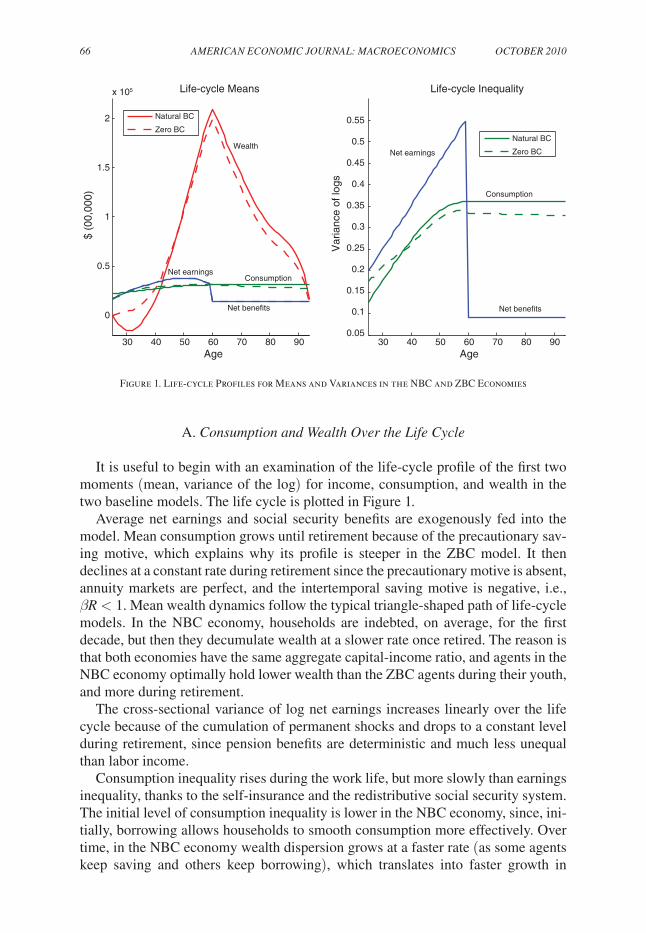
It is useful to begin with an examination of the life-cycle profile of the first two moments (mean, variance of the log) for income, consumption, and wealth in the two baseline models. The life cycle is plotted in Figure 1.
Average net earnings and social security benefits are exogenously fed into the model. Mean consumption grows until retirement because of the precautionary sav-ing motive, which explains why its profile is steeper in the ZBC model. It then declines at a constant rate during retirement since the precautionary motive is absent, annuity markets are perfect, and the intertemporal saving motive is negative, i.e., βR < 1. Mean wealth dynamics follow the typical triangle-shaped path of life-cycle models. In the NBC economy, households are indebted, on average, for the first decade, but then they decumulate wealth at a slower rate once retired. The reason is that both economies have the same aggregate capital-income ratio, and agents in the NBC economy optimally hold lower wealth than the ZBC agents during their youth, and more during retirement.
The cross-sectional variance of log net earnings increases linearly over the life cycle because of the cumulation of permanent shocks and drops to a constant level during retirement, since pension benefits are deterministic and much less unequal than labor income.
Consumption inequality rises during the work life, but more slowly than earnings inequality, thanks to the self-insurance and the redistributive social security system. The initial level of consumption inequality is lower in the NBC economy, since, ini-tially, borrowing allows households to smooth consumption more effectively. Over time, in the NBC economy wealth dispersion grows at a faster rate (as some agents keep saving and others keep borrowing), which translates into faster growth in
30 40 50 60 70 80 90
2
1.5
1
0.5
0
x 105
Age30 40 50 60 70 80 90
Age
$ (0
0,00
0)Life-cycle Means
0.55
0.5
0.45
0.4
0.35
0.3
0.25
0.2
0.15
0.1
0.05V
aria
nce
of lo
gs
Life-cycle Inequality
Natural BC
Zero BCWealth
ConsumptionNet earnings
Net benefits
Consumption
Net earnings
Net benefits
Natural BC
Zero BC
Figure 1. Life-cycle Profiles for Means and Variances in the NBC and ZBC Economies

VOL. 2 nO. 4 67kAPLAn And VIOLAntE: cOnSUMPtIOn InSURAncE
consumption inequality. In the absence of binding borrowing limits, cross-sectional consumption inequality should remain constant during retirement, as consumption growth would be the same for every agent (and equal to βR). This is essentially the case for the NBC economy, whereas in the ZBC economy the fraction of agents at the constraint gradually rises during retirement, which slowly reduces the cross-sectional consumption dispersion.
B. BPP Insurance coefficients in the data and the Model
We now turn to the insurance coefficients. To be consistent with the BPP approach, when computing insurance coefficients, log consumption and log after-tax earnings are defined as residuals from a common age profile and denoted as (cit, yit).
In all tables and figures that follow, columns labeled “Data BPP” report the BPP empirical estimates (with associated standard errors) from the merged PSID/CEX dataset (1980–1992). Columns labeled “Model BPP” refer to the estimates of the model’s insurance coefficients calculated using the instrumental variables approach described in Section IA, i.e., ϕ BPP x
. The difference between Data BPP and Model BPP is informative on the extent of consumption insurance in the model relative to the data, since these are measured in exactly the same way. In other words, that difference tells us how much consumption insurance there is in the data beyond self-insurance.
Average Insurance coefficients.—Table 1 shows that applying the BPP method-ology to the simulated panel of consumption and income generates insurance coef-ficients of 0.22 for permanent shocks and 0.94 for transitory shocks in the economy with natural borrowing limits (NBC). In the economy with zero borrowing (ZBC), these two coefficients are 0.07 and 0.82, respectively. These numbers compare to estimates of insurance coefficients of 0.36 and 0.95, respectively, in the US data.
Hence, the model generates the right amount of insurance with respect to transi-tory shocks in the NBC economy and 87 percent of its data counterpart in the ZBC economy. In this respect, the model is successful. However, the amount of insur-ance against permanent shocks is substantially less than in the US economy, around 60 percent of its empirical value in the NBC economy and 20 percent in the ZBC economy. In this respect, the model admits substantially less insurance than the US economy against permanent earnings shocks. Even though the BPPestimates are imprecise, the model coefficient for the ZBC economy is outside a 90 percent con-fidence interval around the point estimate.24
C. Accuracy of the BPP Methodology
We now assess the accuracy of the BPP methodology for estimating insurance coefficients. This can be done by comparing the columns labeled “Model BPP”
24 A previous draft contained a welfare calculation, based on Heathcote, Storesletten, and Violante (2008a), which established that the discrepancy between ϕ =0.36 (data) and ϕ =0.23 (model) is equivalent, in welfare terms, to around 3 percent of lifetime consumption.

68 AMERIcAn EcOnOMIc JOURnAL: MAcROEcOnOMIcS OctOBER 2010
and “Model TRUE.” This latter label refers to the model’s insurance coefficients ϕx calculated directly from the realizations of the individual shocks instead of the instruments.
Table 1 reveals that whereas the BPP methodology works extremely well for transitory shocks, it tends to systematically underestimate the amount of insurance for permanent shocks. The bias is very small for the NBC economy, just 0.01, but it is large for the ZBC economy, about 0.16. This result suggests that the unbiased empirical estimate of the insurance coefficient for permanent shocks ϕ BPP η
may be even higher than 0.36, which is the BPP point estimate for the US economy.25
Failure of Orthogonality conditions.—This downward bias in the BPPestimator for permanent shocks is exacerbated in the ZBC economy. The reason for the large bias in ϕ BPP η
is that the orthogonality conditions in (SM) may fail when agents are near the liquidity constraint.26 It turns out that both covariances in (SM) contrib-ute to the negative bias. However, the quantitatively more important factor is that cov(Δcit, εi,t−2) < 0.
To gain intuition for why this covariance may be negative near the borrowing limit, consider a household who receives a negative transitory shock at t−2 (i.e., εt−2 < 0). Such a household would like to borrow (or dissave) to smooth the nega-tive shock. However, for a household close to its borrowing limit, even a small reduction in wealth can have a large expected utility cost because of the possibil-ity of becoming constrained in the future. This smoothing entails an optimal drop in consumption at t−2. The closer agents are to the borrowing constraint, the larger this drop. This leads to a positive expected change in consumption in the next period, i.e., cov(Δct−1, εt−2) < 0 as consumption returns to its baseline level. Since agents prefer smooth paths for consumption, this adjustment takes place gradually and cov(Δct, εt−2) < 0 as well.27
25 Authors’ calculations suggest that the absolute size of biases is largely independent of the level of the true value. Hence, unbiased point estimates of ϕ BPP η
for the US economy, once accounting for the downward bias, could be anywhere between 0.37 and 0.52 depending how constrained US households are.
26 Recall that assumption (SM) is required for identification of insurance coefficients for permanent shocks, but not for transitory shocks.
27 With a longer panel, it may be possible to reduce the downward bias in ϕ BPP η by adding additional lags of
income growth to the instrument. For example, using g t η (yi)=Δyi,t−2 + Δyi,t−1 +Δyit +Δyi,t+1 changes the
required short memory assumption to cov(cit, ηi,t−2)=cov(cit, ηi,t−1)=cov(cit, εi,t−3)=0. The cost of using this modified instrument is the additional year of income data required and the associated increase in measurement error.
Table 1—Results from the Benchmark Models with NBC and ZBC
Permanent shock Transitory shock
Data BPP
Model BPP
Model TRUE
Data BPP
Model BPP
Model TRUE
Natural BC 0.36 0.22 0.23 0.95 0.94 0.94(0.09) (0.04)
Zero BC 0.36 0.07 0.23 0.95 0.82 0.82(0.09) (0.04)
VOL. 2 nO. 4 69kAPLAn And VIOLAntE: cOnSUMPtIOn InSURAncE
Small-Sample Bias.—Even though we have mainly interpreted the data-model discrepancy in the BPP coefficients as a failure of the orthogonality conditions assumed by BPP, there is an additional source of discrepancy. Although in the model’s simulations we use a very large sample, the BPP estimates are based on a smaller sample of about 17,000 household/year observations, or roughly 1,300 households per year. To assess the magnitude of the small-sample bias, we have run 50 simulations of samples with 1,300 households each. The means of both the true and the BPP coefficients are virtually unchanged, so we conclude that the small-sample bias is negligible.
D. Age Profiles of Insurance coefficients
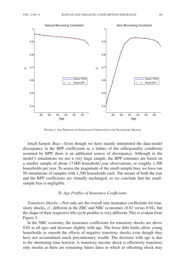
transitory Shocks.—Not only are the overall true insurance coefficients for tran-sitory shocks, ϕε, different in the ZBC and NBC economies (0.82 versus 0.94), but the shape of their respective life-cycle profiles is very different. This is evident from Figure 2.
In the NBC economy, the insurance coefficients for transitory shocks are above 0.85 at all ages and decrease slightly with age. The loose debt limits allow young households to smooth the effects of negative transitory shocks even though they have not accumulated much precautionary wealth. The decrease with age is due to the shortening time horizon. A transitory income shock is effectively transitory only insofar as there are remaining future dates in which an offsetting shock may
30 35 40 45 50 55
Age30 35 40 45 50 55
Age
ϕε ϕε
Natural Borrowing Constraint Zero Borrowing Constraint
Model TRUE
Model BPP
Model TRUE
Model BPP
1
0.9
0.8
0.7
0.6
0.5
0.4
1
0.9
0.8
0.7
0.6
0.5
0.4
Figure 2. Age Profiles of Insurance Coefficients for Transitory Shocks

70 AMERIcAn EcOnOMIc JOURnAL: MAcROEcOnOMIcS OctOBER 2010
be received. This is the horizon effect that we discussed in Section IIIB in reference to the PIH. Finally, note that the BPP estimator is extremely accurate at every age.
When we impose a no-borrowing constraint, the age pattern of the transitory insurance coefficients changes dramatically; it starts at around 0.40 at age 25 and increases sharply in a concave fashion to 0.93 by age 45. As explained, young work-ers have little wealth and cannot borrow. As such, they are unable to smooth negative transitory shocks until they have accumulated enough precautionary savings. Once this point is reached, the profile starts declining as the horizon effect kicks in. In the ZBC case too, the BPP estimator is consistently accurate.
Permanent Shocks.—The true average value of the insurance coefficient ϕη is vir-tually the same in the two economies, 0.23.28 It may seem puzzling that, when bor-rowing constraints are tightened, insurance does not worsen. However, when doing this thought experiment, total wealth is kept constant. Therefore, wealth shifts from old to young households in the form of higher precautionary saving, which increases insurance coefficients for the young.
BPP report that when they allow the insurance coefficient for permanent shocks to vary linearly with age, they estimate a slope that is positive but not significantly different from zero.29 Figure 3 reveals a much starker scenario for both economies. In the NBC economy, ϕ t
η are mildly decreasing at young ages, but are increasing steadily after age 35 and are markedly convex in age. The BPP estimator is always very close to its true value, except at young ages, where agents have the largest debt and are close to their natural limit. The overall shape of the profile in the ZBC economy is similar, except for the initial decrease. As one could have anticipated, the BPP methodology severely underestimates ϕ t
η at young ages, because a large fraction of households is at the constraint. The bias gradually reaches zero only around age 45.
The general shape of the true insurance coefficient is driven by two forces. First, there is the wealth composition effect. As agents accumulate financial wealth, for precautionary and life-cycle reasons, they consume more out of financial wealth and less out of human wealth (i.e., the expected discounted value of their earnings), so permanent shocks to earnings have a smaller impact on consumption. As a result, insurance coefficients have a strong tendency to rise with age. This also explains why, in the NBC economy, insurance coefficients decline in the early part of the life cycle. The deterministically increasing age profile for earnings provides a strong incentive to borrow early in life to smooth consumption, and, as explained, insur-ance coefficients for permanent shocks are increasing in net financial wealth.30
28 This insurance coefficient implies a “marginal propensity to consume” out of permanent shocks of roughly 0.77. Based on his buffer-stock model of consumption, Carroll (2001) explains that the “conventional intuition” that this marginal propensity should be one (as in the strict version of the PIH) is flawed in a life-cycle model.
29 BPP also estimate a larger insurance coefficient for the cohorts born in the 1930s compared to those born in the 1940s but, once again, the difference is statistically insignificant.
30 We have uncovered that the true insurance coefficient ϕ t η may go slightly negative over the first decade. A
negative value for ϕ t η is obtained when cov(Δcit, ηit)>var(ηit), i.e., consumption responds more than one-for-one
to a particular shock. The reason this may happen is due to the interaction of transitory shocks and permanent shocks in the model, as explained by Carroll (1997). With σε >0, households will accumulate a target level of wealth which they use to buffer the effects of transitory shocks. When a positive permanent shock hits, transitory shocks become a smaller component of lifetime income, both in the current period and in all future periods.

VOL. 2 nO. 4 71kAPLAn And VIOLAntE: cOnSUMPtIOn InSURAncE
Second, there is the time horizon effect. By definition, permanent shocks rescale the entire earnings profile during the work life, and also have an effect on retirement income, whose size is inversely proportional to the progressivity of the pension sys-tem. As households get closer to retirement, less of their human wealth is affected in this way by permanent shocks.31
E. Sensitivity Analysis
Tables 2 and 3 report a wide set of sensitivity analysis on the baseline economy with NBC and ZBC, respectively. In each of these experiments, we recalibrate the economy (i.e., we reset β) in order to maintain a wealth-income ratio of 2.5. The corresponding value of β is reported in each row.
The right-hand side of the tables shows that our computed insurance coefficient against transitory shocks is extremely robust across different parameterizations. The left-hand side of the tables reports results for the permanent shock. Allowing for an initial wealth distribution—calibrated on the asset holdings of the young in the
Hence, the utility cost of not being able to smooth transitory shocks falls. Households reduce the optimal level of wealth they desire to buffer transitory shocks. Consumption may thus respond to the full effect of the positive per-manent shock, plus an additional amount that is the decrease in the optimal precautionary wealth level. A similar logic applies to negative permanent shocks. We have verified that when we simulate the model without transitory shocks (σε =0), then ϕ t
η is always positive.31 Interestingly, the true insurance coefficients for both permanent and transitory shock at retirement are equal
(see Figures 2 and 3). In the absence of any pension system (or in presence of the most redistributive system, where benefits are a lump sum disconnected from lifetime earnings), both insurance coefficients at retirement should be approximately one. Since in the model, social security benefits depend also on income in the last year of work, we find that they are both slightly less than one.
Figure 3. Age Profiles of Insurance Coefficients for Permanent Shocks
ϕη ϕη
Age30 35 40 45 50 5530 35 40 45 50 55
Age
Natural Borrowing Constraint Zero Borrowing Constraint
Model TRUE
Model BPP
Model TRUE
Model BPP
1
0.8
0.6
0.4
0.2
0
−0.2
−0.4
−0.6
1
0.8
0.6
0.4
0.2
0
−0.2
−0.4
−0.6

72 AMERIcAn EcOnOMIc JOURnAL: MAcROEcOnOMIcS OctOBER 2010
Table 2—Sensitivity Analysis for the Model with NBC
Permanent shock Transitory shock
Data0.36
(0.09)0.95
(0.04)
Model TRUE Model BPP Model TRUE Model BPP βBenchmark 0.23 0.22 0.94 0.94 0.971
Initial wealth distribution 0.23 0.22 0.94 0.94 0.971
Risk aversion: γ= 1 0.22 0.21 0.94 0.94 0.973 γ= 5 0.27 0.24 0.93 0.93 0.945 γ= 10 0.32 0.29 0.92 0.92 0.855 γ= 15 0.37 0.32 0.92 0.92 0.740
Social security: Replacement ratio = 0.25 0.19 0.17 0.93 0.93 0.958 Replacement ratio = 0.65 0.27 0.26 0.94 0.94 0.982
Variance permanent shock: ση = 0.02 0.25 0.24 0.93 0.93 0.963 ση = 0.005 0.22 0.20 0.94 0.94 0.975 σηage specific 0.24 0.24 0.94 0.94 0.971
Variance initial permanent: σz0 = 0.2 0.23 0.22 0.94 0.94 0.971 σz0 = 0.1 0.24 0.22 0.94 0.94 0.972
Variance transistory shock σε = 0.075 0.24 0.22 0.94 0.94 0.971 σε = 0.025 0.23 0.22 0.94 0.94 0.971
Table 3—Sensitivity Analysis for the Model with ZBC
Permanent shock Transitory shock
Data0.36
(0.09)0.95
(0.04)
Model TRUE Model BPP Model TRUE Model BPP βBenchmark 0.23 0.07 0.82 0.82 0.964
Initial wealth distribution 0.24 0.09 0.83 0.83 0.963
Risk aversion: γ= 1 0.23 0.05 0.81 0.81 0.969 γ= 5 0.23 0.12 0.85 0.85 0.933 γ= 10 0.29 0.19 0.88 0.88 0.838 γ= 15 0.33 0.23 0.88 0.88 0.712
Social security: Replacement ratio = 0.25 0.21 −0.00 0.78 0.78 0.947 Replacement ratio = 0.65 0.25 0.13 0.86 0.85 0.977
Variance permanent shock: ση = 0.02 0.23 0.15 0.83 0.83 0.957 ση = 0.005 0.23 −0.09 0.82 0.82 0.968 σηage specific 0.24 0.08 0.82 0.82 0.964
Variance initial permanent: σz0 = 0.2 0.23 0.07 0.82 0.82 0.964 σz0 = 0.1 0.24 0.08 0.83 0.83 0.965
Variance transitory shock σε = 0.075 0.24 0.00 0.83 0.83 0.963 σε = 0.025 0.23 0.14 0.82 0.82 0.966
VOL. 2 nO. 4 73kAPLAn And VIOLAntE: cOnSUMPtIOn InSURAncE
SCF—has very little effect on the insurance coefficients. Households with high lev-els of risk aversion are less tolerant of consumption fluctuation. Thus, as γ rises, the insurance coefficients for permanent shocks also increase. However, only for values of γ beyond 15, do we reach insurance coefficients close to those estimated in the data. When we reduce the average replacement ratio of the social security system from 0.45 to 0.25, insurance coefficients drop, and when we increase it to 0.65 they increase, as expected.
Interestingly, the amount of insurance in the model does not depend on the size of the shocks when the latter is varied within a plausible range. We also allowed the variance of permanent shocks to be age-specific (we kept its average equal to 0.01), and results are unaltered, i.e., the average insurance coefficient and its age profile are virtually unchanged.32 The reason, as we explain in Section IA, is that ϕη is a “ relative metric,” i.e., it is largely independent of the variance of the shock ση since it is normalized by this variance.
In the NBC economy, the bias in the BPP estimator is always of the same order of magnitude and rather small, except for the high γ case. In the ZBC economy, the bias is always large and particularly so in some cases. For example, with large tran-sitory uncertainty, the borrowing limit will bind more often. With a small replace-ment rate, financial wealth shifts from young workers, who are subject to income shocks, to retirees who are not.
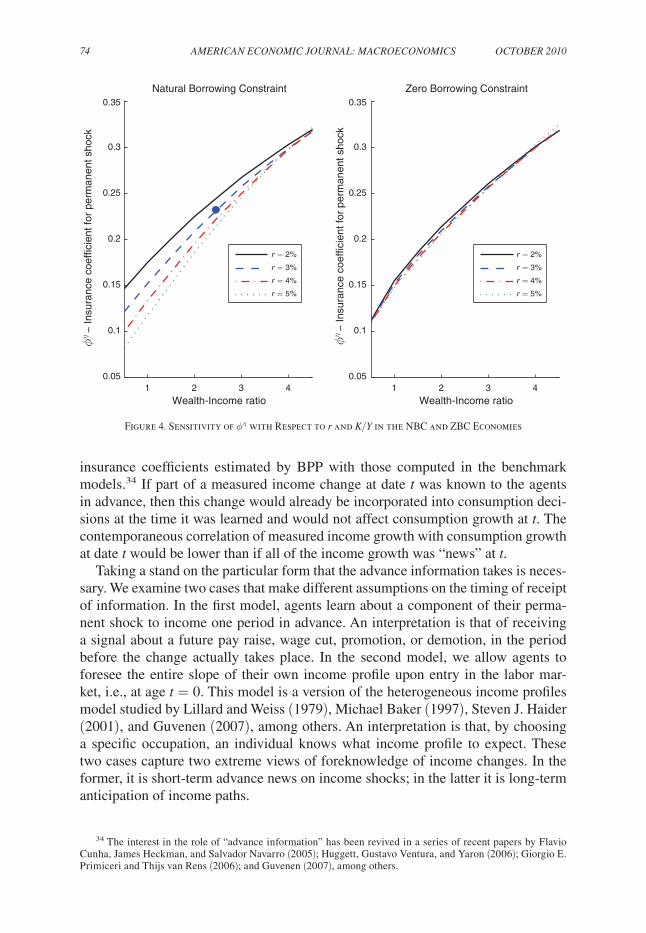
Interest Rate and k/Y Ratio.—Figure 4 plots the values of ϕη as a function of var-ious wealth-income ratios (obtained by changing β) and of various values of r in the two economies. Higher wealth-income ratios map into larger asset holdings that can be used to smooth income shocks, and hence into higher values for ϕη. The idea that patient consumers can self-insure effectively goes back to Menahem E. Yaari (1976) in partial equilibrium and Carroll (1997) and David K. Levine and William R. Zame (2002) in general equilibrium.33 Lower interest rates increase insurance coefficients in the NBC economy, as they loosen the borrowing limit, and the effect is therefore stronger in an economy with low aggregate wealth. In the ZBC economy, lower interest rates reduce the cost of precautionary saving. Qualitatively, consumption smoothing goes up, but we find that quantitatively the effects are negligible.
IV. Advance Information
In this section, we assess whether allowing the agents to know more about their future income growth than the econometrician can reconcile the gap between the
32 Specifically, we used the PSID dataset from Heathcote, Perri, and Violante (2009) to construct a sample of households with the same broad features of the sample selected by BPP for the period 1978–1992. More impor-tantly, we defined income as disposable household income minus financial income, and we dropped records with income growth above 500 percent and below − 80 percent. We estimated the variance of permanent shocks at age a as
σ η a = var(Δyia) + cov(Δyia, Δyi,a−1) + cov(Δyi,a+1, Δyia),
and we smoothed the resulting estimates of σ η a with a cubic polynomial in age. The smooth permanent variances
are markedly U shaped, and the lowest value (around age 45) is roughly half of the highest values, at ages 25 and 60.
33 As expected, we also find that the bias in the BPP coefficient grows as the wealth-income ratios are reduced.
74 AMERIcAn EcOnOMIc JOURnAL: MAcROEcOnOMIcS OctOBER 2010
insurance coefficients estimated by BPP with those computed in the benchmark models.34 If part of a measured income change at date t was known to the agents in advance, then this change would already be incorporated into consumption deci-sions at the time it was learned and would not affect consumption growth at t. The contemporaneous correlation of measured income growth with consumption growth at date t would be lower than if all of the income growth was “news” at t.
Taking a stand on the particular form that the advance information takes is neces-sary. We examine two cases that make different assumptions on the timing of receipt of information. In the first model, agents learn about a component of their perma-nent shock to income one period in advance. An interpretation is that of receiving a signal about a future pay raise, wage cut, promotion, or demotion, in the period before the change actually takes place. In the second model, we allow agents to foresee the entire slope of their own income profile upon entry in the labor mar-ket, i.e., at age t = 0. This model is a version of the heterogeneous income profiles model studied by Lillard and Weiss (1979), Michael Baker (1997), Steven J. Haider (2001), and Guvenen (2007), among others. An interpretation is that, by choosing a specific occupation, an individual knows what income profile to expect. These two cases capture two extreme views of foreknowledge of income changes. In the former, it is short-term advance news on income shocks; in the latter it is long-term anticipation of income paths.
34 The interest in the role of “advance information” has been revived in a series of recent papers by Flavio Cunha, James Heckman, and Salvador Navarro (2005); Huggett, Gustavo Ventura, and Yaron (2006); Giorgio E. Primiceri and Thijs van Rens (2006); and Guvenen (2007), among others.
1 2 3 4
0.35
0.3
0.25
0.2
0.15
0.1
0.05
0.35
0.3
0.25
0.2
0.15
0.1
0.05
Wealth-Income ratio
ϕη −
Insu
ranc
e co
effic
ient
for
perm
anen
t sho
ck
Natural Borrowing Constraint
1 2 3 4Wealth-Income ratio
Zero Borrowing Constraint
r = 2%
r = 3%
r = 4%
r = 5%
r = 2%
r = 3%
r = 4%
r = 5%
ϕη − In
sura
nce
coef
ficie
nt fo
r pe
rman
ent s
hock
Figure 4. Sensitivity of ϕη with Respect to r and K/Y in the NBC and ZBC Economies

VOL. 2 nO. 4 75kAPLAn And VIOLAntE: cOnSUMPtIOn InSURAncE
We are also interested in knowing what the BPP estimator captures in these two cases. BPP are aware that, in the presence of advanced information, their identification strategy may fail and state that, in such case, “the estimated coefficient has to be inter-preted as reflecting a combination of insurance and information” (BPP 2008,1899). We will show that although this is exactly true in the second model, in the first model only the insurance component is reflected in the value of ϕ BPP η
. Put differently, “long-run” foreknowledge seriously compromises identifiability of insurance coefficients of permanent shocks, whereas the “short-run” type makes little difference.
A. Short-run Anticipation of Permanent Shocks
Consider a modification of the information set of the agent whereby the perma-nent change in income at date t, ηit, consists of two additive orthogonal components, η it
s and η it
a . The component η it
s is the true shock that becomes known to the agent only
at date t and affects income at date t. The component η it a is already in the agent’s
information set at date t−1, but it is only incorporated into income at date t. The permanent component of earnings is given by
zit = zi,t−1 + η it s + η it
a ,
where E(η it s ) = E(η it
a ) = 0, and the variances of the two components are varied in a
way that keeps var(ηit) = var(η it s + η it
a ) constant at its baseline value of 0.01.
Permanent Shocks.—In the economy with NBC, from the definition of the insur-ance coefficient for permanent shocks,
(11) ϕη = 1 − cov(Δcit, ηit)_
var (ηit) = 1 −
cov(Δcit, η it s + η it
a )__
var(η it s + η it
a )
= (1 − α)ϕ η s + α ϕ η a
≈ (1 − α)ϕ η s + α,
where ϕ η s and ϕ η a are “insurance coefficients” with respect to the two components of permanent earnings growth (the shock and the change known in advance), and α is the share of the variance of permanent earnings growth that is known one period ahead (i.e., the advance information ratio). The approximate equality in the last line holds because, when borrowing constraints are unimportant, as for the NBC economy, cov(Δcit, η it
a ) ≈ 0, since η it
a is fully incorporated in consumption growth at
t−1. It follows that the true insurance coefficient ϕη is a combination of smoothing (ϕ η s ) and advance information, whose relative magnitude is regulated by α.
However, when the BPP methodology is used to estimate insurance coefficients for permanent shocks, we reach a different conclusion. In what follows, it is useful to ignore the (small in the NBC economy) downward bias discussed in Section IIIC due to the failure of assumption (SM) and associated to the covariance between Δcit and shocks εi,t−2 and η i,t−1 s
.

76 AMERIcAn EcOnOMIc JOURnAL: MAcROEcOnOMIcS OctOBER 2010
From the definition of ϕ BPP η , we have
(12) ϕ BPP η = 1 − cov(Δcit, Δyi,t−1 + Δyit + Δyi,t+1)___cov(Δyit, Δyi,t−1 + Δyit + Δyi,t+1)
≈ 1 − cov(Δcit, η it
s + η i,t+1 a
)__var(η it
s + η it
a )
= 1 − cov(Δcit, η it
s )_
var(η it s ) c var(η it
s )_
var(η it s + η it
a )d
− cov(Δcit, η i,t+1 a
)__var(η it
a ) c var(η it
a )_
var(η it s + η it
a )d
= (1 − α)ϕ η s + αc1 − cov(Δcit, η i,t+1 a
)__var(η it
a ) d
≈ ϕ η s .
The second line uses the fact that cov(Δcit, η it a ) ≈ 0. As evident from the fifth line,
the BPP estimator is a weighted average of the insurance coefficient for the current shock (ϕ η s ) and a term that looks like an insurance coefficient for the component of the t + 1 earnings growth that is known at t. This last term enters the expression through the component Δyi,t+1 of the BPP instrument, i.e., assumption (NF ) fails to hold. Since, in the NBC economy, consumption growth Δcit should react equally to η it
s and to η i,t +1 a
(except for a minor difference due to discounting), we have ϕ BPP η
≈ ϕ η s , as stated in the last line.35
We conclude that, whereas the true insurance coefficient ϕη reflects a combi-nation of insurance and advance information as seen in (11), the BPP coefficient ϕ BPP η
is roughly independent of the amount of foresight. As a result, this form of advance information cannot account for the data-model discrepancy.
transitory Shocks.—For transitory shocks, we have exactly the opposite result. The true insurance coefficients ϕε are unaffected by the presence of advanced infor-mation because the response of consumption growth to transitory shocks is invariant to the timing of news about permanent shocks. However, the BPP estimator ϕ BPP ε has an upward bias that increases with the size of α. To understand this bias, note that
(13) ϕ BPP ε = 1 − cov(Δcit, Δyi,t+1)__cov(Δyit, Δyi,t +1)
= ϕε + cov(Δcit, η i,t+1 a
)__var(εit)
≈ ϕε + α(1 − ϕ η s )cvar(ηit)_var(εit)
d,
35 Katja Kaufmann and Pistaferri (2009) contains a similar derivation of the BPP insurance coefficient in the presence of advance information of this type. However, they assume that all news about ηt+1 accrues before date t. Because of this assumption, they conclude that ϕ BPP η =(1 − α)ϕηs <ϕηs , as is clear from the next-to-last row in (11), and they are led to think that advance information induces an attenuation bias in the BPP estimator.
VOL. 2 nO. 4 77kAPLAn And VIOLAntE: cOnSUMPtIOn InSURAncE
where the second line uses the fact that cov(Δcit, η i,t +1 a )≈cov(Δcit, η it
s ). The
upward bias results from a failure of the identification assumption (NF ), since a fraction of next period permanent income growth in Δyi,t +1 is known in advance and transmits to consumption growth at date t. Quantitatively, this upward bias is small. Since the variance of the permanent innovation is 1/5 of that of transitory shocks, with α = 1/3 the bias would be around 0.05.36
B. Long-Run Foreknowledge of Income Paths
Consider a generalization of the income process in (5) that includes heteroge-neous slopes in individual income profiles:
yit = βi t + zit + εit
zit = zi,t−1 + ηit,
with E(βi) = 0 in the cross section, and var(βi) = σβ.37 We assume that βi is in the information set of the agents at age zero. In the experiments that follow, we keep σε as in the benchmark calibration, gradually change the value for σβ, and set ση residu-ally so that the overall rise in the cross-sectional variance of log earnings from age 25 to age 60 is unchanged.
The results of this experiment for the two economies are reported in Table 4. To get a sense of the size of advance information in each experiment, in the first column of Table 4 we report the fraction of the variance in log earnings at age 60 that is already known by the agents upon entering the labor market.38
The true insurance coefficients for permanent and transitory shocks (ϕη, ϕε) are unchanged from the benchmark model. The reason is that the full effect of knowl-edge about βi is incorporated into the level consumption from the outset, but insur-ance coefficients are a measure of how much consumption growth responds to contemporaneous shocks. This response is not affected by the presence of heteroge-neous slopes known at t = 0.
We now turn to the implications for the BPP coefficients. Table 4 shows that the downward bias in the BPP estimator decreases (and eventually becomes positive) as the amount of advance information is increased. The source of this additional upward bias is as follows. Ignoring the usual sources of downward bias due to the failure of assumption (SM ), the BPP insurance coefficient is given by
36 Simulations confirm these results and show that in the ZBC economy, the usual severe downward bias is always at work, but qualitatively the findings are the same.
37 We retain the unit root specification for the permanent component of the income process, notwithstanding the empirical evidence for substantially lower persistence when heterogeneous slopes are present. We do this to provide a clean analysis of the effects of heterogeneous slopes without confounding the effects of lower persis-tence. We separately analyze the issue of persistence in Section V.
38 The fraction of dispersion at age t known at birth is computed as (σβt 2 )/var(yit).

78 AMERIcAn EcOnOMIc JOURnAL: MAcROEcOnOMIcS OctOBER 2010
(14) ϕ BPP η = 1 −
cov(Δcit, Δyi,t−1 + Δyit + Δyi,t+1)___cov(Δyit, Δyi,t−1 + Δyit + Δyi,t+1)
= 1 − cov(Δcit, ηit + 3βi)__var(ηit) + 3var(βi)
= (1 − α)ϕη + αc1 − cov(Δcit, βi)_
var(βi) d
≈ (1 − α)ϕη + αϕβ,
where α = 3var(βi)/[var(ηit) + 3var(βi)] is another version of the advance informa-tion ratio.
In the NBC model, the term ϕβ is close to one, since Δcit should be roughly invariant to βi at any t. This is a source of upward bias in the BPP estimator, and the bias is larger the larger is α. However, Table 4 shows that only in the case where 80 percent of the variance of income at age 60 is known already at age 25, arguably an upper bound for advance information, is the BPP coefficient in the model at the level of its empirical counterpart.39
In the ZBC economy, ϕβ is close to zero. This induces a further source of down-ward bias, which worsens as one increases the amount of advance information in the economy. As σβ grows, the economy is populated by a larger fraction of agents with steep income profiles who would like to borrow against their future income but are liquidity constrained. As already explained, the larger the fraction of constrained agents, the stronger the downward bias.
V. Persistent Income Shocks
Following BPP, we have focused on a particular income process that restricts shocks to be either fully permanent or fully transitory. There is no scope for income
39 In the NBC model, as the fraction of information known in advance approaches 100 percent, the BPP estimator should approach 1.0. Simulations confirm this prediction.
Table 4—Results for the Model with Heterogeneous Income Slopes
Permanent shock Transitory shock
0.36(0.09)
0.95(0.04)
βData Model TRUE Model BPP Model TRUE Model BPP
Natural BC 40 percent 0.23 0.25 0.94 0.94 0.975 60 percent 0.23 0.28 0.94 0.94 0.978 80 percent 0.22 0.37 0.94 0.94 0.980
Zero BC 40 percent 0.23 − 0.01 0.82 0.82 0.966 60 percent 0.23 − 0.10 0.82 0.82 0.968 80 percent 0.23 − 0.31 0.82 0.82 0.969

VOL. 2 nO. 4 79kAPLAn And VIOLAntE: cOnSUMPtIOn InSURAncE
shocks that have lasting but not permanent effects on income. In this section, we relax this assumption. One plausible explanation for why we find higher insurance coefficients in the data than in the model is that, in reality, shocks are not purely permanent. Persistent shocks are easier to smooth by precautionary saving and borrowing.
Consider a variant of the income process whereby zt follows an AR(1) process with parameter ρ < 1:
(15) zit = ρzit−1 + ηit.
In the terminology of the more general model in equation (1), we now have a0= (1, 1) and aj= (ρj, 0)′, j ≥0.
Identification.—With this income process, the identification strategy of Section IA is no longer valid. We propose two new g t
x (y) functions that identify the two insur-ance coefficients for x = {η, ε}. In order to do this, we assume that an external esti-mate of ρ is available.40
Define the quasi-difference of log income as ˜
Δ yt ≡yt − ρyt−1. Identification of the two insurance coefficients can be achieved by setting g t
ε (y) = ˜
Δ yt +1 and g t η (y)
= ρ2
Δ yt−1 + ρ ˜
Δ yt + ˜
Δ yt +1. For the transitory shock, we have
cov(
Δ yit, ˜
Δ yi,t +1) = − ρvar (εit),
cov(Δcit, ˜
Δ yi,t +1) = − ρcov(Δcit, εit),
and for the persistent shock,
cov(
Δ yit, ρ2
Δ yi,t−1 + ρ ˜
Δ yit + ˜
Δ yi,t+1) = ρvar(ηit),
cov(Δcit, ρ2
Δ yi,t−1 + ρ ˜
Δ yit + ˜
Δ yi,t+1) = ρcov(Δcit, ηit).
Thus, in both cases, expression (4) yields a consistent estimator of ϕx, under exactly the same pair of assumptions (NF ) and (SM ).
Results.—In Table 5, we present insurance coefficients from the NBC and the ZBC models, where zit follows the process in (15). As we decrease ρ, we increase ση in order to keep the rise in the variance of log earnings over the life cycle unchanged and equal to the data counterpart. The column headed “Model TRUE” reports insurance coefficients calculated using the realized values of the shocks. The col-umn headed “Model BPP” reports estimates using the estimation procedure just described. Finally, the column headed “Model BPP Misspecified” reports the esti-mates that would obtain if one were to use the (invalid) instruments from the model
40 This is a reasonable assumption, since p can be identified using panel data on income alone, and thus can be estimated in a separate first stage, before the estimation of insurance coefficients. Obviously, with short panels, distinguishing between a unit root and a stationary but very persistent AR(1) is challenging.

80 AMERIcAn EcOnOMIc JOURnAL: MAcROEcOnOMIcS OctOBER 2010
with permanent shocks. This last column is the correct model counterpart of the BPP estimates.
The coefficients obtained with the misspecified BPP (2008)instruments are very close to those obtained with the correct instruments, at all levels of ρ. This is true for the models both with and without tight borrowing constraint, so the bias that results from applying the instruments from the permanent shock case on data generated by an AR(1) process, is not at all severe. It is thus justified to take the empirical BPP estimate of 0.36 seriously, even in the case where it was estimated under a misspeci-fied income process.
Of course, it is still true that the BPP methodology underestimates true insurance coefficients, but the bias is not increased by the income process misspecification. On the contrary, in the ZBC economy, as ρ decreases, the downward bias in the BPP estimator vanishes. With shocks that are less durable than the unit root, precautionary savings are more useful. Agents start accumulating wealth right away and move far from the debt constraint early in life, which explains why the bias is now very small.
The insurance coefficients for persistent shocks quickly increase as ρ declines. In the NBC economy, with an autoregressive parameter as high as 0.97, the amount of insurance against persistent shocks in the model is roughly consistent with that in the data. In the ZBC economy, not surprisingly, one needs to lower ρ somewhat further, to 0.93. These findings imply that a model economy with a highly persistent (but not permanent) income process can generate, on average, the right level of insurance against persistent shocks.
Turning to insurance coefficients for the transitory shocks, here the model with persistent shocks is slightly less successful. The reason for why the model generates less smoothing with respect to transitory shocks is that now agents shift the use of savings from the smoothing of transitory shocks to the smoothing of persistent shocks, and are willing to tolerate larger fluctuations in consumption due to transi-tory shocks.
Table 5—Results from the Models with Persistent Earnings Shocks
Persistent shock Transitory shock
0.36(0.09)
0.95(0.04)
DataModel TRUE
Model BPP
Model BPP
misspecifiedModel TRUE
Model BPP
Model BPP
misspecified βNatural BC: ρ = 0.99 0.30 0.28 0.28 0.93 0.93 0.93 0.966 ρ = 0.98 0.35 0.34 0.34 0.93 0.93 0.92 0.963 ρ = 0.97 0.39 0.39 0.39 0.93 0.93 0.92 0.960 ρ = 0.95 0.47 0.46 0.46 0.93 0.93 0.90 0.955 ρ = 0.93 0.52 0.53 0.52 0.92 0.93 0.88 0.953
Zero BC: ρ = 0.99 0.27 0.17 0.16 0.82 0.82 0.82 0.960 ρ = 0.98 0.30 0.24 0.22 0.82 0.82 0.81 0.955 ρ = 0.97 0.33 0.28 0.27 0.81 0.81 0.81 0.951 ρ = 0.95 0.38 0.35 0.33 0.81 0.81 0.80 0.945 ρ = 0.93 0.42 0.42 0.38 0.81 0.82 0.78 0.940

VOL. 2 nO. 4 81kAPLAn And VIOLAntE: cOnSUMPtIOn InSURAncE
Figure 5 plots the age profiles of insurance coefficients for persistent shocks in the two economies. Relative to the model with permanent shocks, the age profile of insurance coefficients is now less steep (and thus more consistent with the data). This is because the difference between a permanent and a highly persistent shock is more pertinent for a young household with many periods ahead.
Age-Wealth Profiles.—Even though the model with ρ < 1 is, on average, suc-cessful in replicating the BPP estimates, the age profile is too steep relative to the data. The model has too little insurance for young agents and too much for old agents. Figure 6 provides an explanation for this result. In the data, the distribution of wealth is much less concentrated at retirement than in the model.
In this paper, we have chosen to focus on the baseline life-cycle model with stan-dard preferences and income risk alone, and make a first step toward understanding the data-model gap. Extensions of the SIM model that incorporate saving motives for young (e.g., down payment constraints) and for older households (e.g., bequest) would shift wealth in the right way and help the model to reproduce flatter age-insurance profiles. Additional precautionary saving associated to medical expendi-tures shocks and survival risk would also work, qualitatively, in the right direction (Hubbard, Skinner, and Zeldes 1995).41 Similarly, allowing for a consumption floor in the budget constraint—a simple way to capture some US social insurance program—would mechanically increase consumption smoothing for the poor. The
41 A key difficulty is that the BPP measures of consumption include out-of-pocket medical expenses, which are usually modeled as part of the budget constraint but not in preferences.
30 35 40 45 50 55
1
0.8
0.6
0.4
0.2
0
−0.2
−0.4
−0.6
1
0.8
0.6
0.4
0.2
0
−0.2
−0.4
−0.6
Age30 35 40 45 50 55
Age
ϕηNatural Borrowing Constraint
ϕη
Zero Borrowing Constraint
Model TRUE
Model BPP missp.
Model TRUE
Model BPP missp.
ρ= 0.97
ρ= 1
ρ= 0.93
ρ= 1
Figure 5. Age Profiles of Insurance Coefficients in the NBC and ZBC Economies
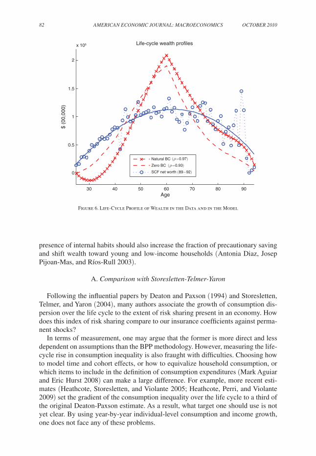
82 AMERIcAn EcOnOMIc JOURnAL: MAcROEcOnOMIcS OctOBER 2010
presence of internal habits should also increase the fraction of precautionary saving and shift wealth toward young and low-income households (Antonia Diaz, Josep Pijoan-Mas, and Ríos-Rull 2003).
A. comparison with Storesletten-telmer-Yaron
Following the influential papers by Deaton and Paxson (1994) and Storesletten, Telmer, and Yaron (2004), many authors associate the growth of consumption dis-persion over the life cycle to the extent of risk sharing present in an economy. How does this index of risk sharing compare to our insurance coefficients against perma-nent shocks?
In terms of measurement, one may argue that the former is more direct and less dependent on assumptions than the BPP methodology. However, measuring the life-cycle rise in consumption inequality is also fraught with difficulties. Choosing how to model time and cohort effects, or how to equivalize household consumption, or which items to include in the definition of consumption expenditures (Mark Aguiar and Eric Hurst 2008) can make a large difference. For example, more recent esti-mates (Heathcote, Storesletten, and Violante 2005; Heathcote, Perri, and Violante 2009) set the gradient of the consumption inequality over the life cycle to a third of the original Deaton-Paxson estimate. As a result, what target one should use is not yet clear. By using year-by-year individual-level consumption and income growth, one does not face any of these problems.
Figure 6. Life-Cycle Profile of Wealth in the Data and in the Model
30 40 50 60 70 80 90
2
1.5
1
0.5
0
x 105
Age
$ (0
0,00
0)
Life-cycle wealth profiles
Natural BC
Zero BC
SCF net worth (89−92)
(ρ=0.97)(ρ=0.93)
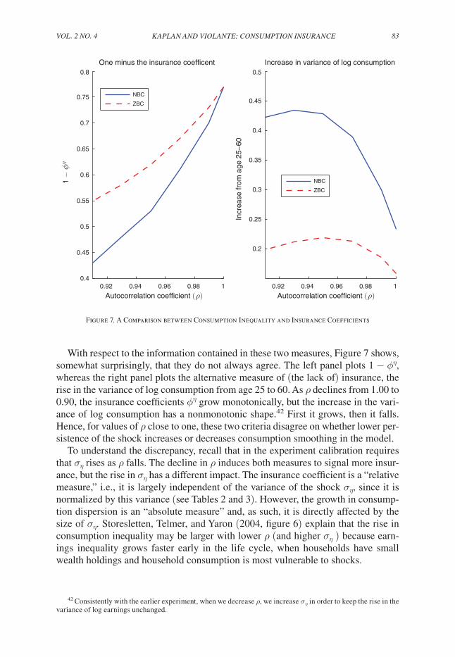
VOL. 2 nO. 4 83kAPLAn And VIOLAntE: cOnSUMPtIOn InSURAncE
With respect to the information contained in these two measures, Figure 7 shows, somewhat surprisingly, that they do not always agree. The left panel plots 1 − ϕη, whereas the right panel plots the alternative measure of (the lack of) insurance, the rise in the variance of log consumption from age 25 to 60. As ρ declines from 1.00 to 0.90, the insurance coefficients ϕη grow monotonically, but the increase in the vari-ance of log consumption has a nonmonotonic shape.42 First it grows, then it falls. Hence, for values of ρ close to one, these two criteria disagree on whether lower per-sistence of the shock increases or decreases consumption smoothing in the model.
To understand the discrepancy, recall that in the experiment calibration requires that ση rises as ρ falls. The decline in ρ induces both measures to signal more insur-ance, but the rise in ση has a different impact. The insurance coefficient is a “relative measure,” i.e., it is largely independent of the variance of the shock ση, since it is normalized by this variance (see Tables 2 and 3). However, the growth in consump-tion dispersion is an “absolute measure” and, as such, it is directly affected by the size of ση. Storesletten, Telmer, and Yaron (2004, figure 6) explain that the rise in consumption inequality may be larger with lower ρ (and higher ση ) because earn-ings inequality grows faster early in the life cycle, when households have small wealth holdings and household consumption is most vulnerable to shocks.
42 Consistently with the earlier experiment, when we decrease ρ, we increase ση in order to keep the rise in the variance of log earnings unchanged.
0.92 0.94 0.96 0.98 1
0.8
0.75
0.7
0.65
0.6
0.55
0.5
0.45
0.4
0.5
0.45
0.4
0.35
0.3
0.25
0.2
Autocorrelation coefficient (ρ)0.92 0.94 0.96 0.98 1
Autocorrelation coefficient (ρ)
1 −
ϕηOne minus the insurance coefficent
NBC
ZBC
Incr
ease
from
age
25−
60
Increase in variance of log consumption
NBC
ZBC
Figure 7. A Comparison between Consumption Inequality and Insurance Coefficients

84 AMERIcAn EcOnOMIc JOURnAL: MAcROEcOnOMIcS OctOBER 2010
VI. Conclusions
This paper is inspired by the important empirical findings by BPP. BPP estimate that, in the US economy, 36 percent of the variance of permanent income shocks and 95 percent of the variance of transitory shocks to after-tax household earnings is insured away by households, i.e., do not translate into contemporaneous consump-tion growth. These two numbers, we argue, should become central in quantitative macroeconomics. They represent a yardstick to measure whether current incom-plete-markets macroeconomic models used for quantitative analysis admit the right amount of household insurance.
In this paper, we make a step forward in this direction by addressing two ques-tions. First, is the standard incomplete-markets (SIM) model—arguably the work-horse of heterogeneous agents macroeconomics—able to replicate such findings? In this respect, our paper is an investigation into one of the central properties of these models. Second, does the BPP methodology provide an unbiased estimator of true insurance coefficients, under the hypothesis that the US economy is accurately described by a SIM model? In this respect, the paper is an investigation into the reliability of the most up-to-date and exhaustive empirical measure of consumption insurance for US households.
We have found that when the log-income process is the sum of a permanent and a transitory component, as assumed by BPP, then a plausibly calibrated environment where households self-insure by trading a risk-free bond displays less consumption insurance than the data against permanent shocks, and about the same as the data against transitory shocks. The model’s shortcoming is particularly stark in environ-ments when borrowing limits are tight. We have shown that this conclusion is robust across a series of sensitivity analysis, including allowing for advance information. We have also shown that allowing for a mean-reverting shock with autocorrelation around 0.95, instead of the permanent component, goes a long way toward reconcil-ing model and data.
We have also assessed the accuracy of the estimation method proposed by BPP by generalizing their approach and clarifying that its validity depends on two key orthog-onality conditions: “no foresight,” and “short memory” of the consumption growth allocation. Estimates of insurance coefficients are, in general, downward biased, with the bias exacerbated whenever households are close to their borrowing constraint. Put differently, the actual insurability of shocks in the US economy may be higher than what was measured by BPP, especially for young and poor households. Moreover, we also showed that in an economy with loose borrowing limits, where the income process contains an individual-specific slope known to the agent (a case of “long-run foreknowledge”), there is a strong source of upward bias in the BPP estimator which stems from the violation of the no advance information assumption. Perhaps surpris-ingly, if the income process is misspecified—as a unit root instead of a very persistent AR(1)—the BPP identification method works very well.
Our investigation suggests several important avenues for future research.Extending the empirical and theoretical analysis to different income definitions
(e.g., hourly wages, individual earnings, pre-government household earnings) would shed light on the relative importance of the various insurance mechanisms

VOL. 2 nO. 4 85kAPLAn And VIOLAntE: cOnSUMPtIOn InSURAncE
to which households have access, beyond self-insurance through borrowing/saving (e.g., individual labor supply, intra-household insurance, government redistribution, interpersonal transfers).43
The question that motivates our paper—whether the standard incomplete-mar-kets model built around “self-insurance” features the right amount of consumption smoothing—could be approached differently. For example, one could rely on the large literature on the consumers’ response to tax rebates (Souleles 1999, Shapiro and Slemrod 2003) to replicate in detail one of the latest refunds (2001 or 2008) and compare the model’s prediction to the econometric and survey-based estimates.
The misalignment between the age profile of insurance coefficients in the model and the data is particularly acute for young individuals. This suggests that modifica-tions of the model that flatten its age-wealth profile, bringing it closer to the data, would also improve its performance in this dimension. Alternatively, future research should try to identify additional sources of insurance against permanent shocks for the young, over and above borrowing and saving. Greg Kaplan (2008), who explores the role of co-residence decisions for unskilled youths, is a promising example.
Finally, future research should explore whether endogenously incomplete-mar-kets models (e.g., environments with limited enforcement or private information) can replicate the two key BPP empirical estimates of the degree of household insur-ance against permanent and transitory shocks. Krueger and Perri (2005), Attanasio and Pavoni (2007), Kruegr and Perri (2008), and Tobias Broer (2009) already made progress in this direction.
REFERENCES
Abowd, John M., and David Card. 1989. “On the Covariance Structure of Earnings and Hours Changes.” Econometrica, 57(2): 411–45.
Aguiar, Mark, and Eric Hurst. 2008. “Deconstructing Lifecycle Expenditure.” Unpublished.Altonji, Joseph G., and Aloysius Siow. 1987. “Testing the Response of Consumption to Income
Changes with (Noisy) Panel Data.” Quarterly Journal of Economics, 102(2): 293–328.Attanasio, Orazio, and Steven J. Davis. 1996. “Relative Wage Movements and the Distribution of
Consumption.” Journal of Political Economy, 104(6): 1227–62.Attanasio, Orazio, and Nicola Pavoni. 2007. “Risk Sharing in Private Information Models with Asset
Accumulation: Explaining the Excess Smoothness of Consumption.” Unpublished.Baker, Michael. 1997. “Growth-Rate Heterogeneity and the Covariance Structure of Life-Cycle Earn-
ings.” Journal of Labor Economics, 15(2): 338–75.Blundell, Richard, and Ian Preston. 1998. “Consumption Inequality and Income Uncertainty.” Quar-
terly Journal of Economics, 113(2): 603–40.Blundell, Richard, Luigi Pistaferri, and Ian Preston. 2008. “Consumption Inequality and Partial
Insurance.” American Economic Review, 98(5): 1887–1921.Broer, Tobias. 2009. “Partial Insurance with Limited Commitment.” Unpublished.Campbell, John Y., and Angus Deaton. 1989. “Why Is Consumption So Smooth?” Review of Eco-
nomic Studies, 56(3): 357–73.Carroll, Christopher D. 1997. “Buffer-Stock Saving and the Life Cycle/Permanent Income Hypoth-
esis.” Quarterly Journal of Economics, 112(1): 1–55.Carroll, Christopher D. 2001. “Precautionary Saving and the Marginal Propensity to Consume out of
Permanent Income.” National Bureau of Economic Research Working Paper 8233.Carroll, Christopher D. 2006. “The Method of Endogenous Gridpoints for Solving Dynamic Stochas-
tic Optimization Problems.” Economics Letters, 91(3): 312–20.
43 Heathcote, Perri, and Violante (2009) document the time-series of cross-sectional US inequality in all these different definitions of income, and in consumption, since the late 1960s.

86 AMERIcAn EcOnOMIc JOURnAL: MAcROEcOnOMIcS OctOBER 2010
Castaneda, Ana, Javier Diaz-Gimenez, and José-Víctor Ríos-Rull. 2003. “Accounting for the U.S. Earnings and Wealth Inequality.” Journal of Political Economy, 111(4): 818–57.
Cochrane, John H. 1991. “A Simple Test of Consumption Insurance.” Journal of Political Economy, 99(5): 957–76.
Cunha, Flavio, James Heckman, and Salvador Navarro. 2005. “Separating Uncertainty from Hetero-geneity in Life Cycle Earnings.” Oxford Economic Papers, 57(2): 191–261.
Deaton, Angus. 1991. “Saving and Liquidity Constraints.” Econometrica, 59(5): 1221–48.Deaton, Angus, and Christina Paxson. 1994. “Intertemporal Choice and Inequality.” Journal of Polit-
ical Economy, 102(3): 437–67.Diaz, Antonia, Josep Pijoan-Mas, and José-Víctor Ríos-Rull. 2003. “Precautionary Savings and
Wealth Distribution under Habit Formation Preferences.” Journal of Monetary Economics, 50(6): 1257–91.
Dynarski, Susan, and Jonathan Gruber. 1997. “Can Families Smooth Variable Earnings?” Brookings Papers on Economic Activity, (1): 229–303.
Fisher, Jonathan D., and David S. Johnson. 2006. “Consumption Mobility in the United States: Evi-dence from Two Panel Data Sets.” B. E. Journal of Economic Analysis and Policy: topics in Eco-nomic Analysis and Policy, 6(1): 1–36.
Gouveia, Miguel, and Robert P. Strauss. 1994. “Effective Federal Individual Income Tax Functions: An Exploratory Empirical Analysis.” national tax Journal, 47(2): 317–39.
Guvenen, Fatih. 2007. “Learning Your Earning: Are Labor Income Shocks Really Very Persistent?” American Economic Review, 97(3): 687–712.
Guvenen, Fatih, and Burhanettin Kuruscu. 2009. “A Quantitative Analysis of the Evolution of the U.S. Wage Distribution: 1970–2000.” In nBER Macroeconomics Annual 2009, Volume 24, ed. Daron Acemoglu, Kenneth Rogoff, and Michael Woodford, 227–76. Chicago: University of Chi-cago Press.
Haider, Steven J. 2001. “Earnings Instability and Earnings Inequality of Males in the United States: 1967–1991.” Journal of Labor Economics, 19(4): 799–836.
Hall, Robert E., and Frederic S. Mishkin. 1982. “The Sensitivity of Consumption to Transitory Income: Estimates from Panel Data on Households.” Econometrica, 50(2): 461–81.
Heathcote, Jonathan, Fabrizio Perri, and Giovanni L. Violante. 2010. “Unequal We Stand: An Empirical Analysis of Economic Inequality in the United States, 1967–2006.” Review of Eco-nomic dynamics, 13(1): 15–51.
Heathcote, Jonathan, Kjetil Storesletten, and Giovanni L. Violante. 2005. “Two Views of Inequality over the Life Cycle.” Journal of the European Economic Association, 3(2–3): 765–75.
Heathcote, Jonathan, Kjetil Storesletten, and Giovanni L. Violante. 2007. “Consumption and Labour Supply with Partial Insurance: An Analytical Framework.” Centre for Economic and Policy Research (CEPR) Discussion Paper 6280.
Heathcote, Jonathan, Kjetil Storesletten, and Giovanni L. Violante. 2008a. “Insurance and Opportu-nities: A Welfare Analysis of Labor Market Risk.” Journal of Monetary Economics, 55(3): 501–25.
Heathcote, Jonathan, Kjetil Storesletten, and Giovanni L. Violante. Forthcoming. “The Macroeco-nomic Implications of Rising Wage Inequality in the United States.” Journal of Political Economy.
Heathcote, Jonathan, Kjetil Storesletten, and Giovanni L. Violante. 2009. “Quantitative Macroeco-nomics with Heterogeneous Households.” Annual Review of Economics, 1(1): 319–54.
Hubbard, R. Glenn, Jonathan Skinner, and Stephen P. Zeldes. 1995. “Precautionary Saving and Social Insurance.” Journal of Political Economy, 103(2): 360–99.
Huggett, Mark. 1993. “The Risk-Free Rate in Heterogeneous-Agent Incomplete-Insurance Econo-mies.” Journal of Economic dynamics and control, 17(5–6): 953–69.
Huggett, Mark. 1996. “Wealth Distribution in Life-Cycle Economies.” Journal of Monetary Eco-nomics, 38(3): 469–94.
Huggett, Mark, Gustavo Ventura, and Amir Yaron. 2006. “Human Capital and Earnings Distribution Dynamics.” Journal of Monetary Economics, 53(2): 265–90.
Imrohoroglu, Ayse, Selahattin Imrohoroglu, and Douglas H. Joines. 1995. “A Life Cycle Analysis of Social Security.” Economic theory, 6(1): 83–114.
Kaplan, Greg. 2008. “Moving Back Home: Insurance Against Labor Market Risk.” Unpublished.Kaufmann, Katja, and Luigi Pistaferri. 2009. “Disentangling Insurance and Information in Intertem-
poral Consumption Choices.” American Economic Review, 99(2): 387–92.Kimball, Miles S. 1990. “Precautionary Saving in the Small and in the Large.” Econometrica, 58(1):
53–73.

VOL. 2 nO. 4 87kAPLAn And VIOLAntE: cOnSUMPtIOn InSURAncE
Krueger, Dirk, and Fabrizio Perri. 2005. “Understanding Consumption Smoothing: Evidence from the U.S. Consumer Expenditure Data.” Journal of the European Economic Association, 3(2–3): 340–49.
Krueger, Dirk, and Fabrizio Perri. 2006. “Does Income Inequality Lead to Consumption Inequality? Evidence and Theory.” Review of Economic Studies, 73(1): 163–93.
Krueger, Dirk, and Fabrizio Perri. 2008. “How Do Households Respond to Income Changes?” Unpublished.
Levine, David K., and William R. Zame. 2002. “Does Market Incompleteness Matter?” Economet-rica, 70(5): 1805–39.
Lillard, Lee A., and Yoram Weiss. 1979. “Components of Variation in Panel Earnings Data: Ameri-can Scientists, 1960–70.” Econometrica, 47(2): 437–54.
Mace, Barbara J. 1991. “Full Insurance in the Presence of Aggregate Uncertainty.” Journal of Politi-cal Economy, 99(5): 928–56.
MaCurdy, Thomas E. 1982. “The Use of Time Series Processes to Model the Error Structure of Earn-ings in a Longitudinal Data Analysis.” Journal of Econometrics, 18(1): 83–114.
Mitchell, Olivia S., and John W. R. Phillips. 2006. “Social Security Replacement Rates for Alterna-tive Earnings Benchmarks.” Benefits Quarterly, (4): 37–47.
Primiceri, Giorgio E., and Thijs van Rens. 2006. “Heterogeneous Life-Cycle Profiles, Income Risk and Consumption Inequality.” Centre for Economic and Policy Research (CEPR) Discussion Paper 5881.
Ríos-Rull, José-Víctor. 1995. “Models with Heterogeneous Agents.” In Frontiers of Business cycles Research, ed. Thomas F. Cooley, 98–125. Princeton: Princeton University Press.
Sargent, Thomas J. 1978. “Rational Expectations, Econometric Exogeneity, and Consumption.” Jour-nal of Political Economy, 86(4): 673–700.
Shapiro, Matthew D., and Joel Slemrod. 2003. “Consumer Response to Tax Rebates.” American Eco-nomic Review, 93(1): 381–96.
Skinner, Jonathan. 1987. “A Superior Measure of Consumption from the Panel Study of Income Dynamics.” Economics Letters, 23(2): 213–16.
Souleles, Nicholas S. 1999. “The Response of Household Consumption to Income Tax Refunds.” American Economic Review, 89(4): 947–58.
Storesletten, Kjetil, Christopher I. Telmer, and Amir Yaron. 2004. “Consumption and Risk Sharing over the Life Cycle.” Journal of Monetary Economics, 51(3): 609–33.
Wolff, Edward N. 1999. “The Size Distribution of Wealth in the United States: A Comparison among Recent Household Surveys.” In Wealth, Work, and Health: Innovations in Measurement in the Social Sciences: Essays in Honor of F. thomas Juster, ed. James P. Smith and Robert J. Willis, 209–32. Ann Arbor: University of Michigan Press.
Yaari, Menahem E. 1976. “A Law of Large Numbers in the Theory of Consumer’s Choice under Uncertainty.” Journal of Economic theory, 12(2): 202–17.

This article has been cited by:
1. A. Fuster, P. S. Willen. 2011. Insuring Consumption Using Income-Linked Assets. Reviewof Finance . [CrossRef]
2. Tullio Jappelli, Luigi Pistaferri. 2011. Financial Integration and Consumption Smoothing*.The Economic Journal no-no. [CrossRef]