SANDIA REPORTSAND2010-3628Unlimited ReleasePrinted June 2010

SIRHEN: a data reduction programfor photonic Doppler velocimetrymeasurementsTommy Ao and Daniel H. Dolan

Prepared bySandia National LaboratoriesAlbuquerque, New Mexico 87185 and Livermore, California 94550

Sandia National Laboratories is a multi-program laboratory operated by Sandia Corporation,a wholly owned subsidiary of Lockheed Martin Corporation, for the U.S. Department of Energy’sNational Nuclear Security Administration under contract DE-AC04-94AL85000.

Approved for public release; further dissemination unlimited.

Issued by Sandia National Laboratories, operated for the United States Department of Energyby Sandia Corporation.

NOTICE: This report was prepared as an account of work sponsored by an agency of the UnitedStates Government. Neither the United States Government, nor any agency thereof, nor anyof their employees, nor any of their contractors, subcontractors, or their employees, make anywarranty, express or implied, or assume any legal liability or responsibility for the accuracy,completeness, or usefulness of any information, apparatus, product, or process disclosed, or rep-resent that its use would not infringe privately owned rights. Reference herein to any specificcommercial product, process, or service by trade name, trademark, manufacturer, or otherwise,does not necessarily constitute or imply its endorsement, recommendation, or favoring by theUnited States Government, any agency thereof, or any of their contractors or subcontractors.The views and opinions expressed herein do not necessarily state or reflect those of the UnitedStates Government, any agency thereof, or any of their contractors.

Printed in the United States of America. This report has been reproduced directly from the bestavailable copy.

Available to DOE and DOE contractors fromU.S. Department of EnergyOffice of Scientific and Technical InformationP.O. Box 62Oak Ridge, TN 37831

Telephone: (865) 576-8401Facsimile: (865) 576-5728E-Mail: reports@adonis.osti.govOnline ordering: http://www.osti.gov/bridge

Available to the public fromU.S. Department of CommerceNational Technical Information Service5285 Port Royal RdSpringfield, VA 22161

Telephone: (800) 553-6847Facsimile: (703) 605-6900E-Mail: orders@ntis.fedworld.govOnline ordering: http://www.ntis.gov/help/ordermethods.asp?loc=7-4-0#online

DE

PA

RT

MENT OF EN

ER

GY

• • UN

IT

ED

STATES OFA

M

ER

IC

A

2

SAND2010-3628Unlimited ReleasePrinted June 2010

SIRHEN: a data reduction programfor photonic Doppler velocimetry measurements

Tommy AoDaniel H. Dolan

Dynamic Material Properties

Sandia National LaboratoriesP.O. Box 5800

Albuquerque, NM 87185

Abstract

SIRHEN (Sandia InfraRed HEtrodyne aNalysis) is a program for reducing data from photonicDoppler velocimetry (PDV) measurements. SIRHEN uses the short-time Fourier transform methodto extract velocity information. The program can be run in MATLAB (2008b or later) or as aWindows executable.

3

Acknowledgments

The authors would like to thank following people for obtaining the data used to test the SIRHENprogram: Aaron Bowers and Andy Shay for building the targets, Randy Hickman and Jesse Lynchfor operating the gas gun, and Sheri Payne for fielding the PDV diagnostic.

4

Contents

1 Introduction 11

1.1 Program summary . . . . . . . . . . . . . . . . . . . . . . . . . . . . . . . . . . . . . . . . . . . . . . . . . . . 12

1.2 Overview of report . . . . . . . . . . . . . . . . . . . . . . . . . . . . . . . . . . . . . . . . . . . . . . . . . . . 12

2 Theoretical background 13

2.1 Photonic Doppler velocimetry . . . . . . . . . . . . . . . . . . . . . . . . . . . . . . . . . . . . . . . . . . 13

2.1.1 Displacement mode . . . . . . . . . . . . . . . . . . . . . . . . . . . . . . . . . . . . . . . . . . . . 13

2.1.2 Velocity mode . . . . . . . . . . . . . . . . . . . . . . . . . . . . . . . . . . . . . . . . . . . . . . . . 16

2.2 Analysis . . . . . . . . . . . . . . . . . . . . . . . . . . . . . . . . . . . . . . . . . . . . . . . . . . . . . . . . . . . 16

2.2.1 Window functions . . . . . . . . . . . . . . . . . . . . . . . . . . . . . . . . . . . . . . . . . . . . . 17

2.2.2 Peak finding methods . . . . . . . . . . . . . . . . . . . . . . . . . . . . . . . . . . . . . . . . . . 21

2.3 PDV configurations . . . . . . . . . . . . . . . . . . . . . . . . . . . . . . . . . . . . . . . . . . . . . . . . . . 26

2.3.1 Standard . . . . . . . . . . . . . . . . . . . . . . . . . . . . . . . . . . . . . . . . . . . . . . . . . . . . 26

2.3.2 Frequency-conversion . . . . . . . . . . . . . . . . . . . . . . . . . . . . . . . . . . . . . . . . . . 26

3 Program overview 29

3.1 Installing and running SIRHEN . . . . . . . . . . . . . . . . . . . . . . . . . . . . . . . . . . . . . . . . . 29

3.1.1 MATLAB version . . . . . . . . . . . . . . . . . . . . . . . . . . . . . . . . . . . . . . . . . . . . . 29

3.1.2 Windows executable . . . . . . . . . . . . . . . . . . . . . . . . . . . . . . . . . . . . . . . . . . . 30

3.2 Analysis outline . . . . . . . . . . . . . . . . . . . . . . . . . . . . . . . . . . . . . . . . . . . . . . . . . . . . 30

3.3 Graphical user interface . . . . . . . . . . . . . . . . . . . . . . . . . . . . . . . . . . . . . . . . . . . . . . . 33

3.3.1 Figures . . . . . . . . . . . . . . . . . . . . . . . . . . . . . . . . . . . . . . . . . . . . . . . . . . . . . . 33

3.3.2 Menu bar . . . . . . . . . . . . . . . . . . . . . . . . . . . . . . . . . . . . . . . . . . . . . . . . . . . . 33

5

3.3.3 Toolbar . . . . . . . . . . . . . . . . . . . . . . . . . . . . . . . . . . . . . . . . . . . . . . . . . . . . . 36

4 Using SIRHEN 39

4.1 Standard PDV examples . . . . . . . . . . . . . . . . . . . . . . . . . . . . . . . . . . . . . . . . . . . . . . 39

4.1.1 Velocity step . . . . . . . . . . . . . . . . . . . . . . . . . . . . . . . . . . . . . . . . . . . . . . . . . 39

4.1.2 Velocity ramp . . . . . . . . . . . . . . . . . . . . . . . . . . . . . . . . . . . . . . . . . . . . . . . . 45

4.2 Frequency-conversion PDV examples . . . . . . . . . . . . . . . . . . . . . . . . . . . . . . . . . . . . 51

4.2.1 Velocity step . . . . . . . . . . . . . . . . . . . . . . . . . . . . . . . . . . . . . . . . . . . . . . . . . 51

4.2.2 Velocity ramp . . . . . . . . . . . . . . . . . . . . . . . . . . . . . . . . . . . . . . . . . . . . . . . . 51

5 Summary 61

5.1 Program features . . . . . . . . . . . . . . . . . . . . . . . . . . . . . . . . . . . . . . . . . . . . . . . . . . . . 61

5.2 Future releases . . . . . . . . . . . . . . . . . . . . . . . . . . . . . . . . . . . . . . . . . . . . . . . . . . . . . . 61

References 62

6

List of Figures

2.1 Conceptual diagram of PDV measurement . . . . . . . . . . . . . . . . . . . . . . . . . . . . . . . . 14

2.2 Window functions . . . . . . . . . . . . . . . . . . . . . . . . . . . . . . . . . . . . . . . . . . . . . . . . . . . 19

2.3 Spectral response of window functions . . . . . . . . . . . . . . . . . . . . . . . . . . . . . . . . . . . 20

2.4 DFT analysis with no zero padding . . . . . . . . . . . . . . . . . . . . . . . . . . . . . . . . . . . . . . 23

2.5 DFT analysis with zero padding . . . . . . . . . . . . . . . . . . . . . . . . . . . . . . . . . . . . . . . . 24

2.6 PDV configurations . . . . . . . . . . . . . . . . . . . . . . . . . . . . . . . . . . . . . . . . . . . . . . . . . . 28

3.1 SIRHEN analysis stages . . . . . . . . . . . . . . . . . . . . . . . . . . . . . . . . . . . . . . . . . . . . . . 31

3.2 SIRHEN operational schematic . . . . . . . . . . . . . . . . . . . . . . . . . . . . . . . . . . . . . . . . . 32

3.3 SIRHEN Selection Screen . . . . . . . . . . . . . . . . . . . . . . . . . . . . . . . . . . . . . . . . . . . . . 34

3.4 SIRHEN Analysis Screen . . . . . . . . . . . . . . . . . . . . . . . . . . . . . . . . . . . . . . . . . . . . . 35

4.1 Example A-1 . . . . . . . . . . . . . . . . . . . . . . . . . . . . . . . . . . . . . . . . . . . . . . . . . . . . . . . 40

4.2 Example A-1 Selection Screen . . . . . . . . . . . . . . . . . . . . . . . . . . . . . . . . . . . . . . . . . 42

4.3 Example A-1 Analysis Screen . . . . . . . . . . . . . . . . . . . . . . . . . . . . . . . . . . . . . . . . . . 43

4.4 Example A-1 extracted velocities . . . . . . . . . . . . . . . . . . . . . . . . . . . . . . . . . . . . . . . 44

4.5 Example A-2 . . . . . . . . . . . . . . . . . . . . . . . . . . . . . . . . . . . . . . . . . . . . . . . . . . . . . . . 47

4.6 Example A-2 Selection Screen . . . . . . . . . . . . . . . . . . . . . . . . . . . . . . . . . . . . . . . . . 48

4.7 Example A-2 Analysis Screen . . . . . . . . . . . . . . . . . . . . . . . . . . . . . . . . . . . . . . . . . . 49

4.8 Example A-2 extracted velocities . . . . . . . . . . . . . . . . . . . . . . . . . . . . . . . . . . . . . . . 50

4.9 Examples B-1 and B-2 . . . . . . . . . . . . . . . . . . . . . . . . . . . . . . . . . . . . . . . . . . . . . . . . 52

4.10 Example B-1 Selection Screen . . . . . . . . . . . . . . . . . . . . . . . . . . . . . . . . . . . . . . . . . . 53

4.11 Example B-1 Analysis Screen . . . . . . . . . . . . . . . . . . . . . . . . . . . . . . . . . . . . . . . . . . 54

7

4.12 Example B-1 extracted velocities . . . . . . . . . . . . . . . . . . . . . . . . . . . . . . . . . . . . . . . . 55

4.13 Example B-2 Selection Screen . . . . . . . . . . . . . . . . . . . . . . . . . . . . . . . . . . . . . . . . . . 57

4.14 Example B-2 Analysis Screen . . . . . . . . . . . . . . . . . . . . . . . . . . . . . . . . . . . . . . . . . . 58

4.15 Example B-2 extracted velocities . . . . . . . . . . . . . . . . . . . . . . . . . . . . . . . . . . . . . . . . 59

8

List of Tables

2.1 Window functions . . . . . . . . . . . . . . . . . . . . . . . . . . . . . . . . . . . . . . . . . . . . . . . . . . . 18

2.2 Peak finding methods . . . . . . . . . . . . . . . . . . . . . . . . . . . . . . . . . . . . . . . . . . . . . . . . . 21

9

10

Chapter 1

Introduction

Time-resolved velocimetry is one of the primary measurements in dynamic material studies. Tra-ditionally, optical diagnostics such as velocity interferometer system for any reflector (VISAR) [1]and Fabry-Perot interferometer system [2] have been used to measure material velocities in shockwave experiments. Each of those diagnostics have their advantages and disadvantages.

In VISAR measurements, Doppler shifted light from a moving target is split along two differentpaths (a reference leg and a delay leg of an interferometer), then recombined and recorded ondigitizers. The velocity of the target is measured by comparing Doppler shifted light at time t withDoppler shifted light at time t− τ , where τ is the delay time. A chief advantage of VISAR is thatlarge velocities (> 1 km/s) can be tracked with modest diagnostic bandwidth. On the other hand,VISAR uses absolute intensities to obtain velocity information which is disadvantageous as thelight intensity changes substantially. Fabry-Perot interferometry is an alternative to VISAR thatis more robust to extreme changes in light intensity, but has lower optical efficiency and is morecostly and complex. Fabry-Perot systems record data on streak cameras which have limited recordlengths and are susceptible to image distortions. The main advantage of the Fabry-Perot systemis its ability to measure multiple discrete velocities simultaneously and velocity dispersion over alimited range, which VISAR cannot do. However, both systems are vulnerable to abrupt velocitychanges and require having an additional backup system to resolve fringe jump ambiguities.

Photonic Doppler velocimetry (PDV), also known as heterodyne velocimetry [3], is a compactdisplacement interferometer system that is rapidly becoming a standard diagnostic in dynamiccompression research. It has many of the advantages of VISAR and the Fabry-Perot systems,while avoiding some their disadvantages. A PDV system is essentially a fiber-based Michelsoninterferometer, utilizing recent advances in near-infrared (λ0 = 1550 nm) detector technology andfast digitizers to record beat frequencies in the gigahertz range. While fluctuations in the lightintensity returned from the surface are observed in the data, PDV is robust against large variations.The use of Fourier transform techniques in the analysis of PDV data enable resolving multiplediscrete velocities and even velocity dispersion. Additional advantages of PDV include simpleassembly and operation, readily available components, and the lack of an intrinsic delay time.

This report describes the new Sandia InfraRed HEtrodyne aNalysis program (SIRHEN; pro-nounced “siren”) that has been developed for efficient and robust analysis of PDV data. The pro-gram was designed for easy use within Sandia’s dynamic compression community.

11

1.1 Program summary

The SIRHEN program is completely self-contained and employs a simple graphical user inter-face (GUI) to guide the user through the analysis process. It is written in MATLAB and canoperate on any platform (Mac OS X, Windows XP/Vista, and Linux) with MATLAB version2008b or later. For non-MATLAB users, a compiled executable is also available for WindowsXP. The SIRHEN program can be obtained by contacting Tommy Ao (tao@sandia.gov) or DanDolan (dhdolan@sandia.gov).

1.2 Overview of report

Chapter 2 provides a theoretical background on photonic Doppler velocimetry and the analysis pro-cedures used in the SIRHEN program. An overview of the operation of SIRHEN and its graphicaluser interface are presented in Chapter 3. In Chapter 4, several example problems are presented togive the user experience with the program. Chapter 5 summarizes the program’s capabilities anddiscusses future releases.

12

Chapter 2

Theoretical background

This chapter reviews theoretical concepts used in the SIRHEN program. First, the conceptualoperation of photonic Doppler velocity is described. Next, the analysis procedures employed inSIRHEN are presented. Finally, various PDV configurations are discussed.

2.1 Photonic Doppler velocimetry

PDV data may be analyzed in terms of either a displacement or a velocity framework [4]. Thedisplacement mode analysis is more fundamental and provides a helpful starting point for thediscussion. However, the velocity mode analysis described in the subsequent section is the actualbasis of operation for the SIRHEN program.

2.1.1 Displacement mode

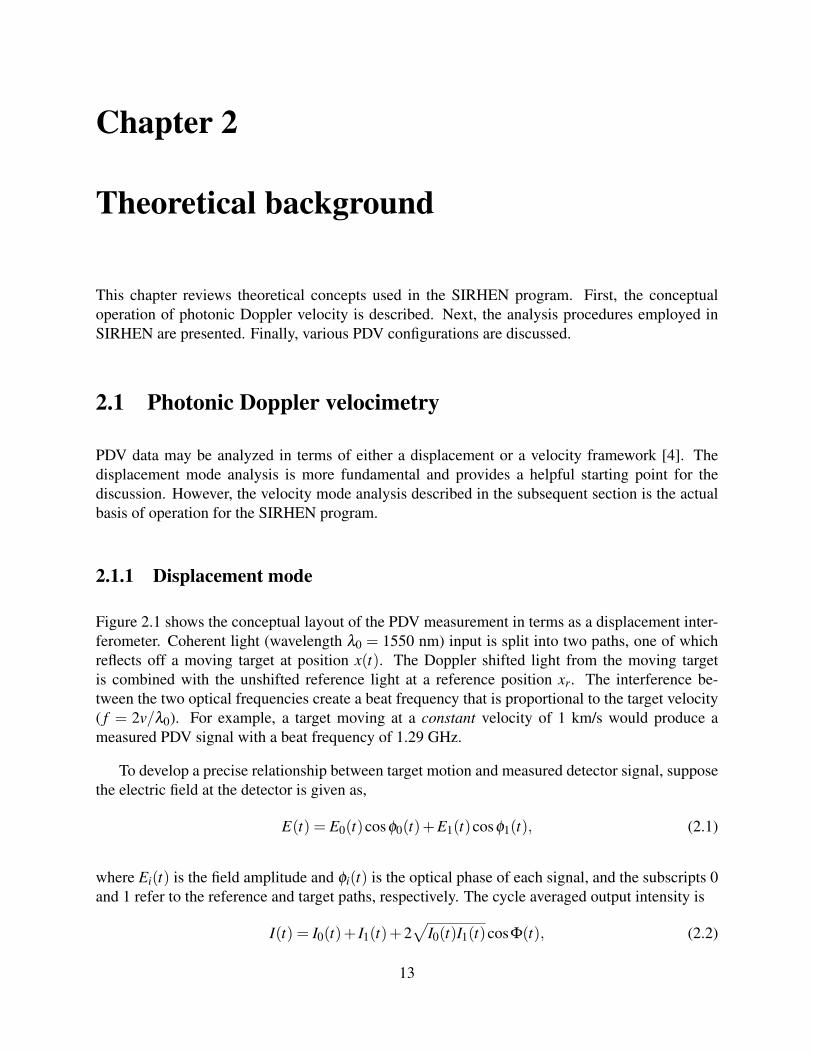
Figure 2.1 shows the conceptual layout of the PDV measurement in terms as a displacement inter-ferometer. Coherent light (wavelength λ0 = 1550 nm) input is split into two paths, one of whichreflects off a moving target at position x(t). The Doppler shifted light from the moving targetis combined with the unshifted reference light at a reference position xr. The interference be-tween the two optical frequencies create a beat frequency that is proportional to the target velocity( f = 2v/λ0). For example, a target moving at a constant velocity of 1 km/s would produce ameasured PDV signal with a beat frequency of 1.29 GHz.

To develop a precise relationship between target motion and measured detector signal, supposethe electric field at the detector is given as,

E(t) = E0(t)cosφ0(t)+E1(t)cosφ1(t), (2.1)

where Ei(t) is the field amplitude and φi(t) is the optical phase of each signal, and the subscripts 0and 1 refer to the reference and target paths, respectively. The cycle averaged output intensity is

I(t) = I0(t)+ I1(t)+2√

I0(t)I1(t)cosΦ(t), (2.2)

13

input

output

target

xr x(t)

v(t)

Figure 2.1. Conceptual diagram of PDV measurement.

14

where the optical phase difference is Φ(t) = φ1(t)−φ0(t), which describes the interference of lighttraveling along the two different paths. The output intensity is recorded using an optical detectorthat converts it to an electrical signal s(t). Changes in optical phase difference lead to variations inthe electrical signal which in turn relate to the motion of the reflecting target. For a monochromaticsource (angular frequency ω0 = 2πc/λ0), the input optical phase is a linear function of time,

φin(t) = ω0t +δin. (2.3)

The reference and reflected optical phases are time delayed versions of the input signal in whichthe reference signal time delay (T0) is constant while the reflected signal time delay (2T1) varieswith the target position. The factor of 2 in the reflected signal delay is due to the round trip transitbetween the reference position xr and the target postion x(t). The output optical phases are givenas,

φ0(t) = φin(t−T0), (2.4)

φ1(t) = φin[t−2T1(t))]−δm, (2.5)

where the phase change caused by reflection δm is assumed to be constant. Referring to Fig. 2.1,the reflection delay time is given as,

T1(t)≈xr− x [t−T1(ti)]

c; (v� c), (2.6)

where T1(ti) is the initial transit time. Omitting the constant time shift between Φ(t) and x(t), theoptical phase difference is related to the target’s position relative to the reference position at timeti,

Φ(t) = Φ(ti)+4πx(t)− x(ti)

λ0, (2.7)

where Φ(ti) is the initial phase difference, and x(ti) = xr. Thus, the electrical signal of a detectormeasuring the output intensity is given as,

s(t) = aI0(t)+bI1(t)+2√

abI0(t)I1(t)cos[

Φ(ti)+4πx(t)− x(ti)

λ0

](2.8)

where the constants a and b represent a collection of coupling factors from the reference and targetpaths, respectively and the detector’s sensitivity. The target displacement can be determined byinverting Eq. 2.8, which may give ambiguous results due to the symmetry and periodicity of thecosine function; similar concerns led to the use of quadrature in VISAR [5]. To obtain velocityinformation, numerical differentiation is required which could result in substantial noise amplifi-cation [6].

15

2.1.2 Velocity mode

Numerical differentiation may be avoided using a velocity mode analysis. When the target un-dergoes a slow velocity change such that over a time interval τ , its instantaneous position may beapproximated as

x(t)≈ x(t)+ v(t)[t− t]; (|t− t| ≤ τ/2) , (2.9)

where v represents the average interval velocity, and t is the center of the time interval. The opticalphase difference within this interval is

Φ(t)≈Φ(t1)−ω(t)[t− t], (2.10)

where ω = 4πv/λ0. The output electrical signal the detector may be given as,

s(t) = Acos(Φ−ω[t− t]

), (2.11)

where ω represents the radial beat frequency within the signal. This frequency can be determinedby calculating the electrical power spectrum using a short-time Fourier transform (STFT),

S(ω, t) =∫

∞

−∞

s(t)w(t)e−iωtdt, (2.12)

where w(t) is a window function, discussed in the following section. At each time of interest twithin an interval of time duration τ , the beat frequency is extracted from the peak of the powerspectrum. The average velocity in each interval is given as

v =λ0

2f =

λ0

4πω, (2.13)

where the velocity resolution is defined by how well the frequency peak can be resolved.

2.2 Analysis

In the SIRHEN program, a discrete Fourier transform (DFT) analysis is used to transform the inputfunction s(t) (detector signal in the time domain) into an output function S( f ) called the frequencydomain representation. DFT is a specific kind of Fourier transform where the input function isdiscrete and whose non-zero values have a limited (finite) duration. This is precisely the type ofdata created by digitizing at a finite sampling rate a continuous PDV electrical signal,

s(t)[Fs]−→ sn, (2.14)

where Fs is the sampling frequency, and sn is the discrete signal. DFTs can be computed efficientlyusing a fast Fourier transform (FFT) algorithm [7].

16

Unlike the discrete-time Fourier transform (DTFT), DFT only evaluates enough frequencycomponents to reconstruct the finite segment that was analyzed. Using the DFT implies that thefinite segment analyzed is one period of an infinitely extended periodic signal. Since that is nottrue of real experimental signals, a window function has to be used to reduce the artifacts in thespectrum. From Eq. 2.12, the previously described STFT analysis can be given as

S( f ) =N−1

∑n=0

snwne−i2π f n, (2.15)

where wn is a discrete window function.

2.2.1 Window functions

Spectral leakage is an effect in frequency analysis of finite-length signals or finite-length segmentsof infinite signals where it appears as if some energy has “leaked” out of the original signal spec-trum into other frequencies. Typically the leakage shows up as a series of frequency “side-lobes”.Windows are weighting functions applied to data to reduce the spectral leakage associated withfinite observation intervals.

When a signal (data) is multiplied by a window function wn, the product is zero-valued outsidethe interval so all that is remains is the signal segment “viewed” through the window. The maincriteria for the spectral response of a window are:

1. the width of the main-lobe,

2. the attenuation at the maximum height of a side-lobe, generally the first side lobe, and

3. the rate at which the peaks of the side-lobes fall-off.

Ideally, the spectral response of the window consists of:

1. a narrow main-lobe (corresponding to high frequency resolution),

2. a low first-side-lobe (corresponding to noise suppression), and

3. rapid fall-off of the remaining side-lobes.

A vast collection of window functions have been developed for DFT analysis [7, 8]. Fourcommon window functions are available in the SIRHEN program: Boxcar, Hann, Hamming, andBlackman, which are shown in Fig. 2.2. The corresponding spectral response of the windowsare shown in Fig. 2.3 and summarized in Table 2.1. The subsequent window descriptions use thefollowing FFT algorithm terminology:

17

• N represents the width (total number of samples) of the discrete window function.

• n is an integer with values: 0≤ n≤ N−1.

Highest Side-lobeWindow Side-lobe Fall Off Comments

Level (dB) (dB/oct)Boxcar -13 -6 sensitive to signal phaseHann -32 -18 preferable with low noise (1%)

Hamming -43 -6 preferable with moderate noise (5-10%)Blackman -58 -18 widest main-lobe

Table 2.1. Spectral response of window functions.

Boxcar

The “Boxcar” or rectangular or Dirichlet window is the simplest window,

wn = 1. (2.16)

It extracts a segment of the signal without any other modification at all, which leads to disconti-nuities at the endpoints. Using a normalized coordinates with sample period T = 1.0 so that ω isperiodic in 2π and hence identified as θ , the spectral response of the Boxcar is given as,

W (θ) = exp(−i

N−12

θ

)sin[N

2 θ]

sin[1

2θ] , (2.17)

whose magnitude is shown in Fig. 2.3(a). The width of its main-lobe is quite narrow, but its first-side-lobe is only −13 dB down from the main-lobe peak and the remaining side-lobes fall-offgradually at about −6 dB/octave.

Hann

The “Hann” or sometimes mistakenly called “Hanning” window is a raised cosine named afterJulius von Hann,

wn = 0.5[

1− cos(

2πnN−1

)]. (2.18)

Not only is this window continuous, but so is its first derivative. As shown in Fig. 2.3(b), its first-side-lobe is −32 dB from the main-lobe peak and has a steeper side-lobe fall-off of about −18dB/octave. However, its main-lobe is wider than the Boxcar’s.

18

N-1

Figure 2.2. Window functions.

19

(a) (b)

(c) (d)

Figure 2.3. Spectral response of window functions: (a) Boxcar,(b) Hann, (c) Hamming, and (d) Blackman.

20

Hamming

The “Hamming” window, proposed by Richard W. Hamming, is also a raised cosine,

wn = 0.54−0.46cos(

2πnN−1

). (2.19)

It is optimized to minimize the first-side-lobe (−43 dB), whose height is about one-tenth that ofthe Hann window’s first-side-lobe, as shown in Fig. 2.3(c). The Hamming window has a main-lobewidth similar to the Hann window, while it has a gradual side-lobe fall-off (−6 dB/octave) like theBoxcar window.

Blackman

R. B. Blackman developed the “Blackman” window,

wn = 0.42−0.5cos(

2πnN−1

)+0.08cos

(4πn

N−1

). (2.20)

As shown in Fig. 2.3(d), its first-side-lobe is down to about −58 dB and has a steep side-lobefall-off (−18 dB/octave), but it also has the widest main-lobe of the 4 described windows.

2.2.2 Peak finding methods

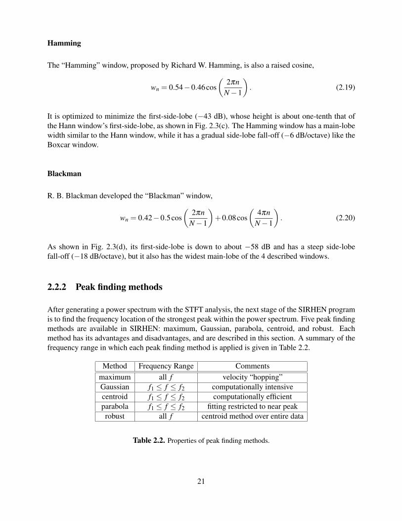
After generating a power spectrum with the STFT analysis, the next stage of the SIRHEN programis to find the frequency location of the strongest peak within the power spectrum. Five peak findingmethods are available in SIRHEN: maximum, Gaussian, parabola, centroid, and robust. Eachmethod has its advantages and disadvantages, and are described in this section. A summary of thefrequency range in which each peak finding method is applied is given in Table 2.2.

Method Frequency Range Commentsmaximum all f velocity “hopping”Gaussian f1 ≤ f ≤ f2 computationally intensivecentroid f1 ≤ f ≤ f2 computationally efficientparabola f1 ≤ f ≤ f2 fitting restricted to near peakrobust all f centroid method over entire data

Table 2.2. Properties of peak finding methods.

21

Maximum

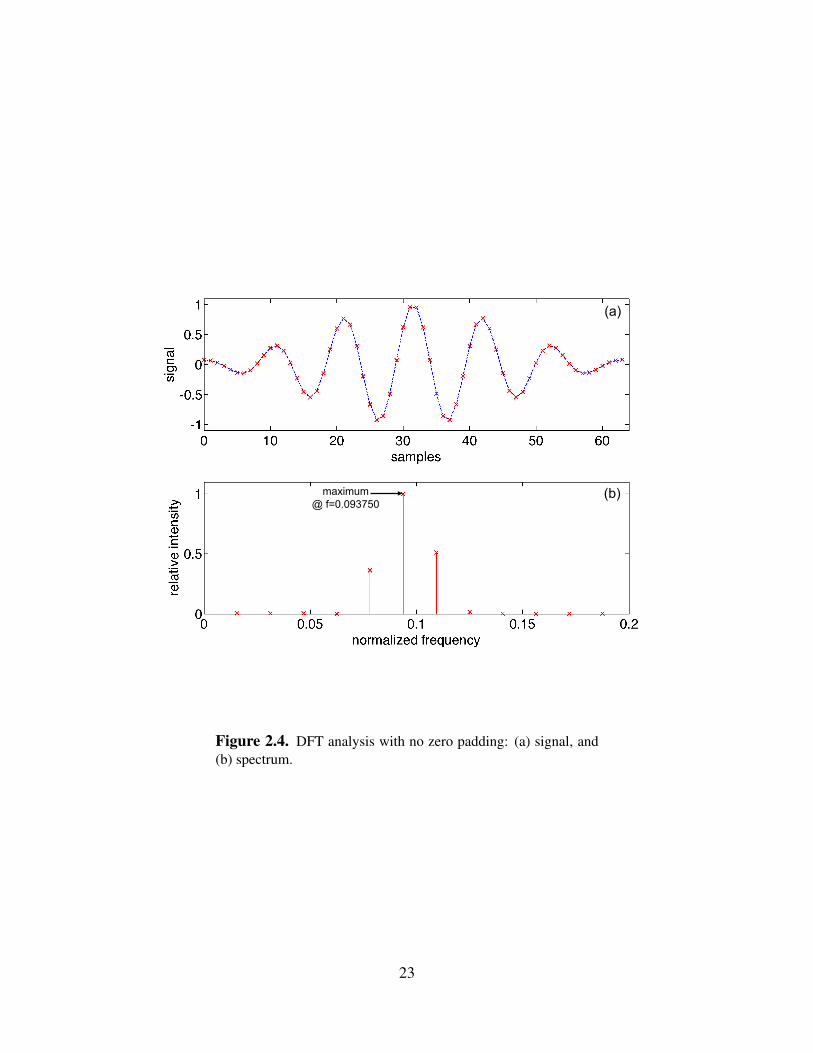
The most obvious peak finding algorithm is to simply locate the frequency of the global maximumwithin the spectrum. While this method will always produce a result, the accuracy of the frequencyvalue is dependent on the number of frequency points used in the STFT calculation. Consider thefollowing example, a sinusoidal signal sampled at N = 64 points,

sn = cos(

2π6n

N−1

), (2.21)

and windowed with a Hamming window function, as shown Fig. 2.4(a). This example signal has anormalized frequency of

f =6

2π(64−1)= 0.095238. (2.22)

Taking a FFT of the signal produces the power spectrum shown Fig. 2.4(b). Because of the limitednumber of sample points in the signal, the spectral peak only contains 3 frequency points. Using themaximum peak finding method, the normalized frequency of the peak is found to be f = 0.093750,which results in peak finding error of ∼ 1.5%.

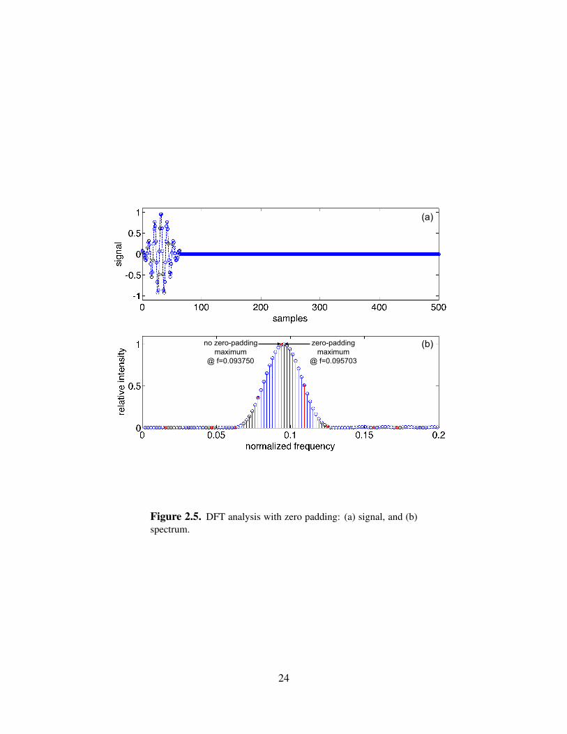
The procedure of appending zero value samples to the end of the signal (in this case Nz = 448points and shown in Fig. 2.5(a)), otherwise known as “zero-padding”, generates more frequencypoints in the spectrum, as shown in Fig. 2.5(b). Because appending zeros does not change the inputsampling rate, Fs, the frequency span of the FFT output will remain the same and evenly distributedset of samples spread over 0 to Fs/2. The sample spacing of the new output must decrease to fitmore samples over the same frequency range and corresponds to a resolution increase in thosesamples. However, it is important to note that only the frequency grid of the analysis is improved,but not the frequency peak width; the only way to do improve the latter is to increase the timeduration of the block of signal that is examined. In any case, using the maximum method again onthe zero-padding signal, a more accurate normalized frequency is obtained, f = 0.095703, whichreduces the peak finding error to ∼ 0.5%.

However, it should also be noted that large amounts of zero-padding slow the analysis consid-erably. In addition, the maximum method has problems during rapid transitions between low andhigh velocities as the intensities of the two different spectral peaks compete in magnitude. Themaximum method tends to “hop” between the two extreme frequency values which producing ajagged velocity history. Thus, other more efficient peak finding methods that provide smoothertransitions have been explored, and made available in the SIRHEN program. The following threemethods (Gaussian, parabola, and centroid) uses an initial maximum method to center ( f0) andlimit the data range ( f1 ≤ f ≤ f2) for their subsequent peak finding algorithms.

22

maximum @ f=0.093750

(a)

(b)

Figure 2.4. DFT analysis with no zero padding: (a) signal, and(b) spectrum.

23

(a)

(b) no zero-padding maximum

@ f=0.093750

zero-padding maximum

@ f=0.095703

Figure 2.5. DFT analysis with zero padding: (a) signal, and (b)spectrum.

24

Gaussian

One of the most widely used peak finding algorithms is to fit the spectral peak with a Gaussiancurve,

S( f ) = Aexp(−( f − f )2

2σ2

)+S0, (2.23)

where the fitting parameters are the amplitude A, the width σ , and the center frequecny f of theGaussian peak, and the background signal level S0. Even using just 3 points within the spectralpeak, the Gaussian method noticeably improves peak frequency location accuracy over the max-imum method. Certainly, having at least a moderate amount of zero-padding to the signal giveseven better results. However, since the algorithm involves 2 linear and 2 nonlinear parameters in aleast squares fitting, it may also be computationally intensive.

Parabola

Another peak finding method fits the spectral peak to a simple polynomial curve, namely a parabola,

S( f ) = A( f − f )2. (2.24)

This fitting algorithm is more efficient than the Gaussian fitting since it uses the built-in polynomialfitting routine of MATLAB on a limited range of data restricted near the peak.

Centroid

Alternatively, instead of fitting the spectral peak to a curve, the profile is integrated to find itscentroid location,

f =

∫ f2

f1f S( f )d f∫ f2

f1S( f )d f

. (2.25)

This method tends to be less sensitive to any skewness in the spectral profile compared to theGaussian and Parabola methods, and is very computationally efficient.

Robust

The final peak finding method, referred to as the “robust” method, uses the above centroid algo-rithm. However, instead of limiting the integrals to within a certain data range ( f1 ≤ f ≤ f2), therobust method applies them over the entire signal.

25

2.3 PDV configurations

2.3.1 Standard

In a typical (standard) PDV configuration, a single laser light source is used to illuminate a tar-get and provide an unshifted reference light for interference with the target light, as shown inFig. 2.6(a). When the target is stationary, no beating within the PDV signal occurs since the re-flected light from the target also remains unshifted.

The relationship between the time duration τ and characteristic peak width ∆ f follows theuncertainly product,

(∆ f )(τ)≥ 14π

. (2.26)

For example, to achieve a velocity precision ∆v = 10 m/s, the minimum time duration neededin the STFT analysis is τ = 6 ns. For measured velocities that are reasonably large (> 1 km/s),the relative velocity precision (∆v/v < 1%) is sufficient to investigate many dynamic materialproperties. However, low velocity (< 100 m/s) transients can be difficult to resolve with standardPDV since the beat period of the feature of interest may be longer than the time duration of theanalysis. Also, in order to improve the poor relative velocity precision (∆v/v ∼ 10% ), τ must beincreased, thus sacrificing time precision.

2.3.2 Frequency-conversion

To provide optimal velocity and time precision measurements, a frequency-conversion PDV con-figuration has recently been developed where the reference light is preset at a slightly differentfrequency (wavelength) than the target light frequency. This is achieved by either using an acousto-optic (AO) frequency shifter to modify the reference light frequency, as shown in Fig. 2.6(b), orby using two separate laser sources at slightly different frequencies, as shown in Fig. 2.6(c). Inthis configuration, the PDV signal contains an underlying beat frequency even when the target isstationary. Thus, the low velocity features now have a shorter beat period than in the standard PDVconfiguration, which enables the use of a small time duration while maintaining sufficient velocityprecision.

Suppose the target light before Doppler shift has wavelength λT , and the reference source haswavelength λR. The phase difference Φ(t) = φT (t)−φR(t), where

φR(t) =2πc0

λRt +δR, (2.27)

φT (t) =2πc0

λT[t−2T (t)]+δT −δm, (2.28)

26

T (t)≈ xr− x(t)c0

, (2.29)

becomes

Φ(t) = 2πc0

[1

λT− 1

λR

]t +

4πx(t)λT

+δT −δm−δR−4πxr

λT. (2.30)

The fringe shift F(t) (defined from a reference position x0 at t = 0) is

F(t) =[

1− λT

λR

]c0tλT

+2

λT(x(t)− x0) . (2.31)

The time derivative of the fringe shift is the apparent frequency of the PDV signal,

dFdt

=[

1− λT

λR

]c0

λT+

2vλT

. (2.32)

Thus, when λT > λR the frequency conversion acts in opposition to the Doppler shift, creatinglower frequencies with increasing velocity (until crossing, at which point the frequency increases).In the opposite case (λT < λR), the frequency increases with positive velocity.

27

1X2

detector

target circulator

fiber coupler

2X1 reference

laser fiber

coupler

(a)

detector

target circulator

2X1 reference

laser 2

laser 1

fiber coupler

(c)

1X2

detector

target

AO frequency

shifter 2X1

reference

laser

fiber coupler

fiber coupler

circulator

(b)

Figure 2.6. PDV configurations: (a) standard, (b) frequency-conversion with AO frequency shifter, and (c) frequency-conversion with 2 lasers.

28

Chapter 3

Program overview

An overview of the SIHREN program is presented in this chapter. First, program installation andexecution instructions are given. Next, the program’s operational stages are defined. Finally, thefeatures of the graphical user interface are presented.

3.1 Installing and running SIRHEN

SIRHEN exists in two formats:

1. MATLAB version which runs within the MATLAB program, and

2. Windows executable version which may be used on Windows systems without the MATLABprogram.

Installation of each version is different and are described separately in the following sections.

3.1.1 MATLAB version

The MATLAB version of SIRHEN is intended for MATLAB version 2008b or later. A valid MAT-LAB license (http://www.mathworks.com) is required. First, copy the folder matlabSIRHEN,which contains all files and subdirectories of the MATLAB version of SIRHEN to a local directoryof the machine. Next, startup the MATLAB program. To install SIRHEN, add the matlabSIRHENdirectory to the MATLAB path, using either the “addpath” command or the “Set path” tool onthe “File” menu. Only the main folder itself, not the private subdirectory, should be added tothe path. After installation is complete, the program can be started by typing “SIRHEN” at thecommand line.

29

3.1.2 Windows executable

The executable version of SIRHEN is intended for Windows XP. The program may operate inolder versions of Windows but is not supported. Also, the executable version of SIRHEN hasnot been tested on Windows Vista and Windows 7 but should presumably work. After the con-tents of the winexe folder has been copied to a local directory of the machine, double click theMCRInstaller2008b.exe program and accept all default choices in the installation. This processinstalls necessary libraries and support functions for SIRHEN, and needs to be performed once foreach machine where the program is to be used. When the MCR installer is complete, SIRHENcan be launched by double clicking on the SIRHEN.exe executable. The initial launch of the pro-gram will be somewhat slow as the various routines are unpacked for the first time, but subsequentlaunches should be considerably faster.

3.2 Analysis outline

Figure 3.1 outlines the analysis stages of the SIRHEN program. The PDV signal is cropped tothe time range of interest for the experiment. The experiment signal is multiplied with a windowfunction and analyzed with a short-time Fourier transform (STFT) over a certain time duration atdiscrete time points to generate a power spectrum of the signal. At each time point, the frequencyof spectral peak is obtained with a peak finding algorithm. The peak frequencies are converted tovelocity values which are collected to form a velocity history of the experiment.

An operational schematic of SIRHEN is shown in Fig. 3.2. All actions of the first stage aredone within the “Selection Screen”, while all actions of the second stage are done in the “AnalysisScreen”. The SIRHEN program opens with the Selection Screen (see Fig. 3.3) and begins with theuser selecting a signal data file to import into SIRHEN with the “Load data” menu action. Afterthe signal data is loaded, it is displayed in the top figure of the Selection Screen. Meanwhile, acoarse STFT is performed on the full signal and its STFT image is presented in the bottom figure.The signal may be shifted along the time axis with the “Shift signal” menu action. The time regionof experimental interest is selected with the “Experiment region” menu action. A time region priorto the experiment region used for a reference calculation is chosen with the “Reference region”menu action.

To continue onto the second stage of operation, the user clicks on the “Next” button whichreplaces the Selection Screen with the Analysis Screen (see Fig. 3.4). The STFT is performed onthe selected experiment region of the signal and its STFT image is displayed in the top figure of theAnalysis Screen. Meanwhile, using a set of default parameters, the velocity history is calculatedfrom the locations of the peaks of the STFT power spectrum and is presented in the bottom figure.Refinement of the velocity history is performed with the “Calculate history” menu action. Thevelocity history is saved as a text file with the “Export history” menu action. The STFT image issaved as a text file with the “Export STFT image” menu action. To go back to the Selection Screen,the user clicks on the “Previous” button.

30

crop signal

PDV signal

power spectrum

experiment signal window function

STFT

peak finding

velocity history

spectral peak

Figure 3.1. SIRHEN analysis stages.

31

Load signal

Selection Screen

Reference region

Experiment region

Shift signal

Calculate history

Export STFT image

Export history

Analysis Screen

next

previous

Figure 3.2. SIRHEN operational schematic.

32

3.3 Graphical user interface

This section describes the graphical user interface (GUI) of SIRHEN, as shown in Figs. 3.3 & 3.4.Each screen has two figures, a menu bar, and a toolbar.

3.3.1 Figures

In the Selection Screen, the top figure displays the loaded PDV signal and the bottom figure showsa STFT image over the full signal. In the Analysis Screen, the top figure displays a STFT imageover the experiment region of the signal and the bottom image shows the corresponding calculatedvelocity history. Right clicking on the vertical axis label of the figures in the Analysis Screenallows the y-axis to be given in terms of absolute frequency, relative frequency, and velocity. Rightclicking on the colorbar allows the display of the STFT image to be adjusted.

3.3.2 Menu bar

Each screen in SIRHEN has the common “Program” menu, “Help” menu, and “Options” menu.Meanwhile, the “Data” menu contains different actions for the separate screens.

Program and Help

The Program menu allows the user to restart and exit the program. “Restart” closes and relaunchesthe program, clearing all entries and returning the program to its default state. “Exit” closes theprogram. The Help menu provides general information about SIRHEN and briefly summarizes theoperations that can be performed.

Options

The Options menu has the following actions:

1. General- Set parameters for PDV wavelength, velocity scale factor, and velocity level offset.

2. STFT- Set parameters for STFT calculation including number of time points, number of frequencypoints, overlap between time durations, window type, normalization, and DC removal.

3. Display- Set parameters for displaying the STFT image including scale range, color scaling, andcolor map.

33

Figure 3.3. SIRHEN Selection Screen.

34

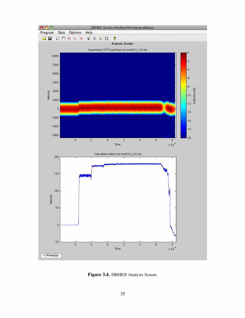
Figure 3.4. SIRHEN Analysis Screen.

35

Data

In the Selection Screen, the Data menu has the following actions:

1. Load signal- Select data file to import into the SIRHEN program. Supported file types include text files(*.txt, *.dat, *.csv), Tektronix binary files (*.wfm), and NTS binary files (*.dig).

2. Shift signal- Signal shifting along time axis (x-axis).

3. Reference region- Select time region for reference calculation.

4. Experiment region- Select time region of experimental interest.

In the Analysis Screen, the Data menu has the following actions:

1. Calculate history- Set parameters for calculating the velocity history including analysis duration, skip interval,minimum number of frequency points, and peak location method.

2. Export history- Save the calculated velocity history to an text file.

3. Export STFT image- Save the STFT image to a text file.

3.3.3 Toolbar

Each screen in SIRHEN contains a toolbar with the following actions:

1. Set working directory- Change the current directory using a dialog box.

2. Save figure- Save figure as a MATLAB *.fig file or a graphic file (*.pdf, *.jpg, etc.).

3. Zoom- Zoom in with mouse click or click and drag.- Zoom out with shift-click; double-click to restore original view.- Press right mouse button (control-click) for additional options.

36

4. Pan- Click and drag to pan over an axes; double-click to restore original view.- Press right mouse button (control-click) for additional options.

5. Auto scale axes- Click on axes to set auto limits.- Shift-click to auto scale all figure axes.

6. Tight scale axes- Click on axes to set tight limit.- Shift-click to tight scale all figure axes.

7. Manual scale axes- Click on axes to manually set limits.

8. Data cursor- Click on data to display (x,y,z) coordinates.- Press right mouse button (control-click) for additional options.

9. Region of interest (ROI) statistics- Click and drag to specify a region of interest.- Local statistics in this region will be displayed.

10. Overlay (x,y) data- Click on axes to overlay (x,y) data from a file.- Right-click overlays to make adjustments.

11. Clone axes- Click on axes to clone to another figure.

12. Toolbar help- Displays the above tools operations.

37

38

Chapter 4

Using SIRHEN

This chapter describes the practical use of the SIRHEN program using several example problems,which are located within the examples directory. The user is guided through the analysis of theseexamples in the following sections. The first section presents examples based on the standard PDVconfiguration, while the second section deals with examples using the frequency-conversion PDVconfiguration. The example data signals are synthesized under ideal conditions: noise-free andover-sampled by a 32-bit digitizer at 10× the Nyquist limit (20 samples/cycle).

4.1 Standard PDV examples

4.1.1 Velocity step

Example A-1 is based on an instantaneous velocity step at time t = 0 from an initial zero velocityto a final velocity v1 = 387.5 m/s (see Fig. 4.1(a)),

v ={

0, t < 0;v1, t ≥ 0.

(4.1)

The example file exA-1.txt contains the synthetic standard PDV signal for this velocity history,as shown in Fig. 4.1(b). Notice when there is no velocity (t < 0), the signal has no beat frequencyand is ideally flat (under noise-free conditions). At t = 0, the signal immediately begins oscillatingat the constant final beat frequency.

After starting the SIRHEN program, load the data file exA-1.txt using the Load signal actionunder the Data menu. The Selection Screen will display the full signal record and an initial STFTanalysis of the signal. Adjust the program by setting the following Data menu parameters:

• Reference region: -Inf, -Inf;

• Experiment region: -5.00e-8, 4.00e-7.

Next, under the Options menu set the following General parameters:

39

(a)

(b)

Figure 4.1. Example A-1 velocity step: (a) velocity profile, and(b) standard PDV signal.

40

• Wavelength: 1.550e-6,

• Velocity scale factor: 1,

• Velocity level offset: 0,

and the following STFT parameters:

• Number time points: 1024,

• Number frequency points: 1024,

• Overlap ratio: 4,

• Window type: Hamming,

• Normalization: global,

• DC removal: no,

and the following Display parameters:

• Scale range (min max): -40 0,

• Color scale: log,

• Color map: jet.

The Selection Screen should now look like Fig. 4.2. Click on the Next button to move to theAnalysis Screen. Under the Data menu, set the following Calculate history parameters:

• Analysis duration: 5.0e-9,

• Skip interval: 2.0e-10,

• Minimum # frequency points: 2048,

• Peak location method: maximum.

The Analysis Screen should look like Fig. 4.3. Under the Data menu, select the Export historyaction to save the extracted velocity profile.

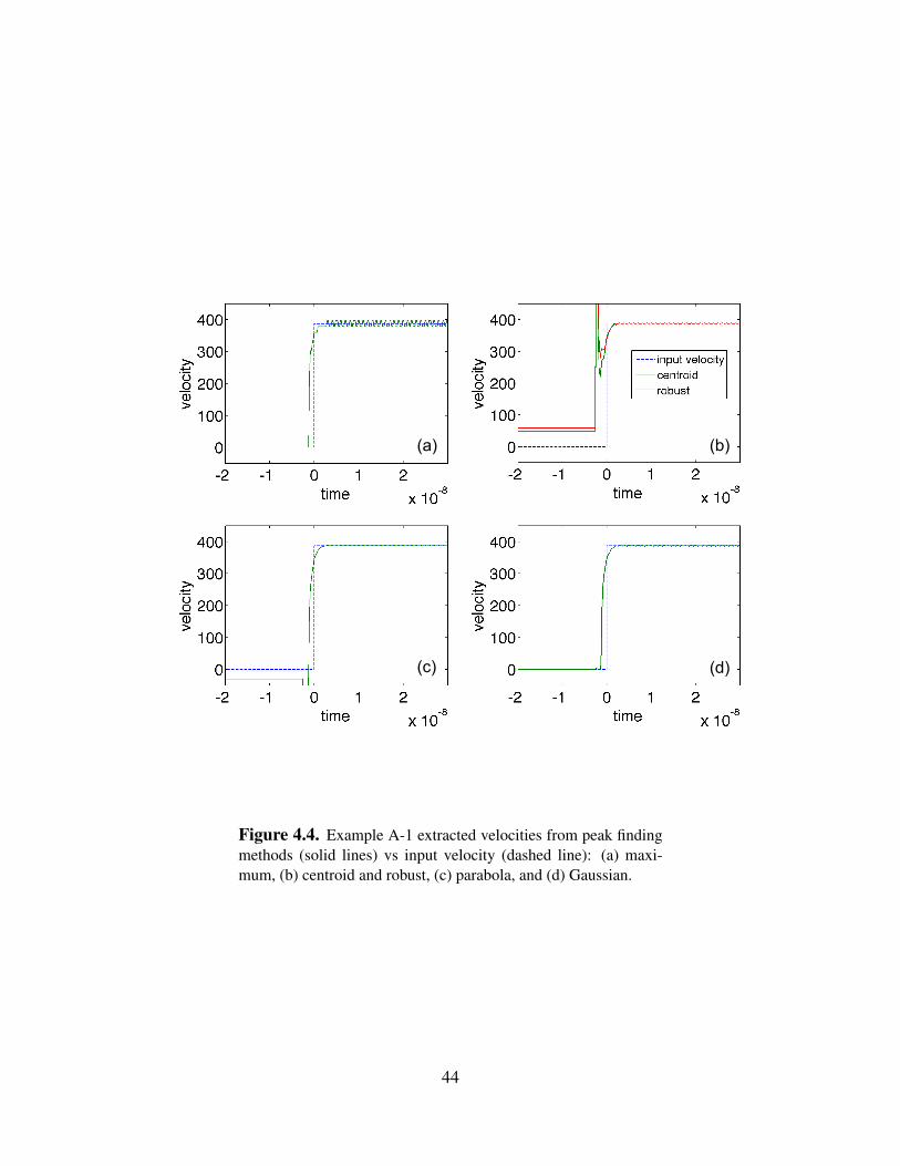
A comparison of the various peak finding methods is shown in Fig. 4.4, where in each caseonly the “Peak location method” parameter was changed. Within each of the subplots, the inputvelocity profile (dashed line) used to obtain the example signal data is also shown. The maximummethod gives the correct zero initial velocity, but has noticeable ringing (oscillations) during the

41

Figure 4.2. Example A-1 Selection Screen.

42

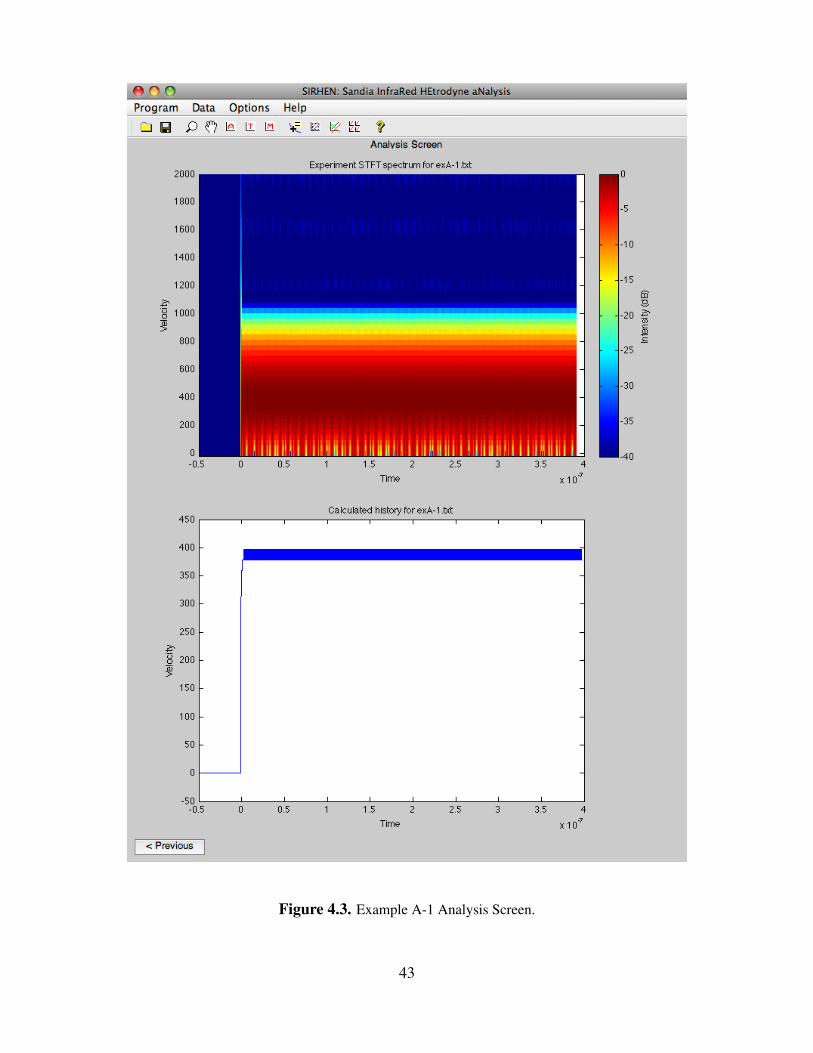
Figure 4.3. Example A-1 Analysis Screen.

43

(c)

(a) (b)

(d)

Figure 4.4. Example A-1 extracted velocities from peak findingmethods (solid lines) vs input velocity (dashed line): (a) maxi-mum, (b) centroid and robust, (c) parabola, and (d) Gaussian.

44

final velocity plateau. The centroid and robust methods both reduce the final velocity ringing,but each has a large positive velocity spike during the step transition and an incorrect positivefinite initial velocity. The parabola method also reduces the final velocity ringing, but has a largenegative velocity spike and an incorrect negative initial velocity. The Gaussian method gives thecorrect zero initial velocity and a relatively flat final velocity.

The risetime of the velocity step is related to the analysis duration used (τ = 5 ns), thus it canbe slightly improved by shrinking the analysis duration. However, the analysis duration should notbe made less than the beat period of the signal which for this example is T = 2 ns.

4.1.2 Velocity ramp

Example A-2 is based on the following linear ramp profile (see Fig. 4.5(a)),

v =

0, t < 0;at, 0≤ t ≤ t1;v1, t > t1.

(4.2)

The example file exA-2.txt contains the synthetic standard PDV signal for this velocity historyunder ideal conditions, as shown in Fig. 4.5(b). Load the example file exA-2.txt, and set thesame program parameters as in the previous example. The Selection Screen should now look likeFig. 4.6.

In the Analysis Screen under the Data menu, set the following Calculate history parameters:

• Analysis duration: 15.0e-9,

• Skip interval: 2.0e-10,

• Minimum # frequency points: 2048,

• Peak location method: maximum.

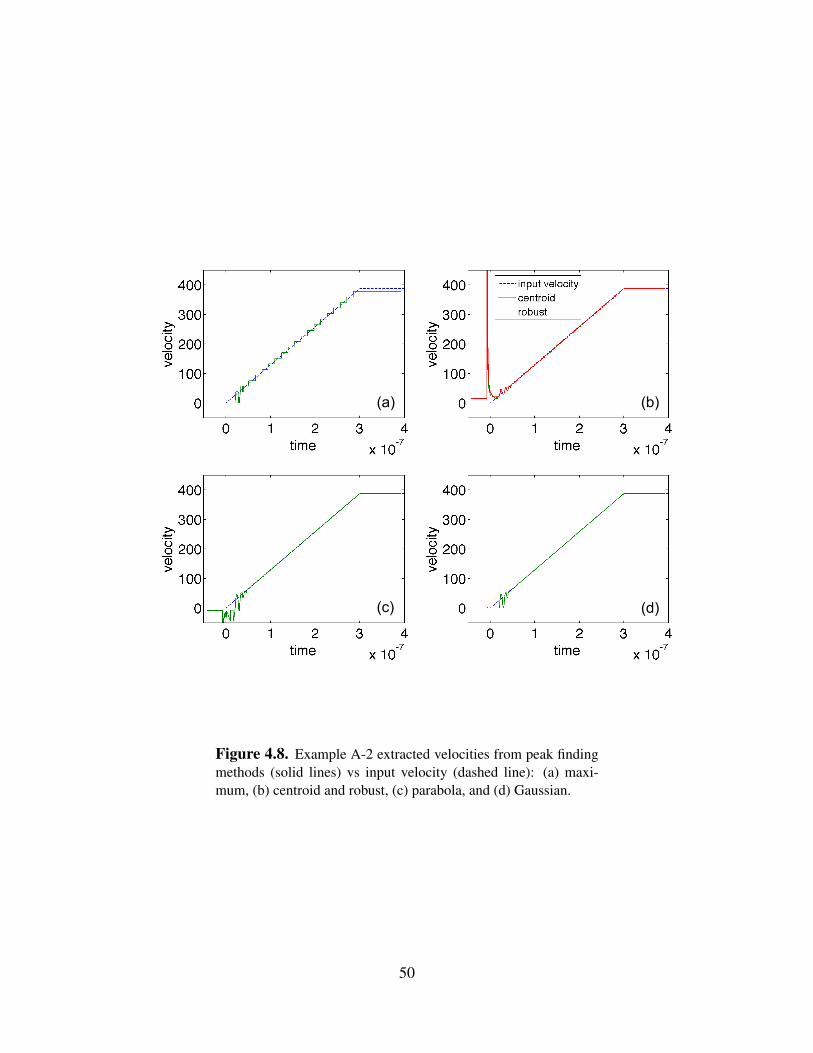
The Analysis Screen should now look like Fig. 4.7. Under the Data menu, select the Export historyaction to save the extracted velocity profile. A comparison of the various peak finding methods isshown in Fig. 4.8, where in each case only the “Peak location method” parameter was changed.The maximum method gives the correct zero initial velocity, but produces large discrete stepswithin the ramp profile and an incorrect low final velocity plateau. Both the centroid and robustmethod reduce the discreteness of the ramp profile and give the correct final velocity, but haveincorrect positive finite initial velocities and positive velocity spikes. The parabola method alsoreduces the discreteness of the ramp profile and gives the correct final velocity, but has an incorrectnegative initial velocity and a negative velocity spike. The Gaussian method gives the correctinitial velocity and final velocity, and a smooth ramp profile, but like all of the other methods hasnoticeable oscillations at low velocities.

45

The inability of all the methods to resolve the low velocity portion of the ramp is really due tothe shortcoming of standard PDV, which consequently has led to the development of frequency-conversion PDV, and illustrated in the next section’s examples.

46

(a)

(b)

Figure 4.5. Example A-2 velocity ramp: (a) velocity profile, and(b) standard PDV signal.

47

Figure 4.6. Example A-2 Selection Screen.

48

Figure 4.7. Example A-2 Analysis Screen.

49

(c)

(a) (b)

(d)

Figure 4.8. Example A-2 extracted velocities from peak findingmethods (solid lines) vs input velocity (dashed line): (a) maxi-mum, (b) centroid and robust, (c) parabola, and (d) Gaussian.

50

4.2 Frequency-conversion PDV examples

As in the previous section, similar velocity step and velocity ramp examples are presented here.However, an underlying beat frequency ( f0 = 0.5 GHz) is now contained within each of the exam-ple PDV signals.

4.2.1 Velocity step

Example B-1 is the frequency-conversion PDV velocity step example. The example file exB-1.txtcontains the frequency-conversion PDV signal for a velocity step, as shown in Fig. 4.9(a). At timest < 0, the signal displays only the underlying beat frequency or “reference frequency” of 0.5 GHz.At t = 0, a noticeable jump in the signal’s frequency is observed at the onset of target motion.Load the example file exB-1.txt, and in the Selection Screen adjust the program by setting thefollowing Data menu parameters:

• Reference region: -9.00e-8, -1.00e-8;

• Experiment region: -5.00e-8, 4.00e-7.

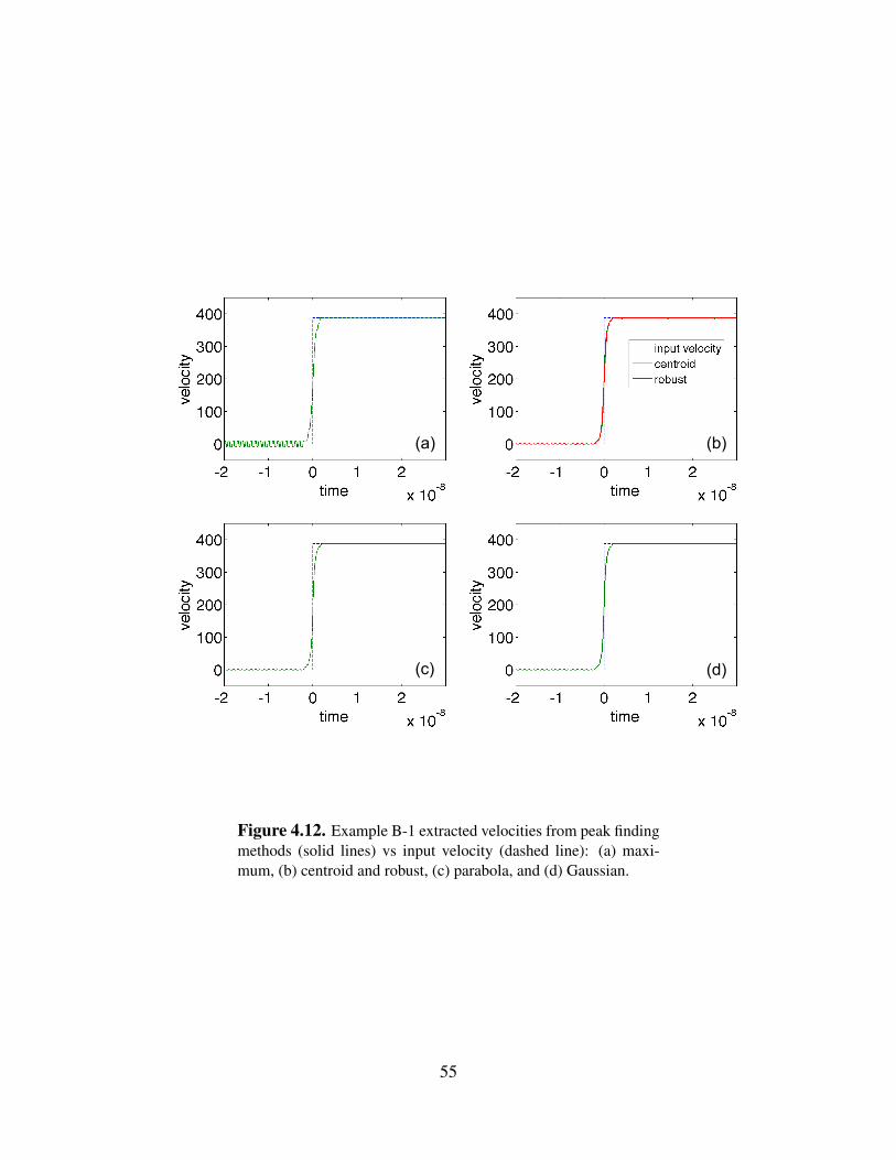
The Selection Screen should look like Fig. 4.10 and the Analysis Screen should look like Fig. 4.11.Under the Data menu, select the Export history action to save the extracted velocity profile. Acomparison of the various peak finding methods is shown in Fig. 4.12, where in each case onlythe “Peak location method” parameter was changed. The maximum method gives the correct finalvelocity, but produces some ringing around the zero initial velocity. The centroid, robust, parabola,and Gaussian methods all reduce the initial ringing and give almost identical velocity profiles.

4.2.2 Velocity ramp

Example B-2 is the frequency-conversion PDV velocity ramp example. The example file exB-2.txtcontains the frequency-conversion PDV signal for a velocity ramp, as shown in Fig. 4.9(b). It mightbe less obvious than the previous step velocity example, but a careful examination does reveal anoticeable increase the signal’s frequency starting at t = 0 due to the onset of target motion. Loadthe example file exB-2.txt, and and set the same program parameters as in the previous example.The Selection Screen should look like Fig. 4.13. In the Analysis Screen under the Data menu, setthe following Calculate history parameters:

• Analysis duration: 15.0e-9,

• Skip interval: 2.0e-10,

• Minimum # frequency points: 2048,

51

(a)

(b)

Figure 4.9. Examples B-1 and B-2: (a) B-1, frequency-conversion PDV signal of velocity step, (b) B-2, frequency-conversion PDV signal of velocity ramp.

52

Figure 4.10. Example B-1 Selection Screen.

53

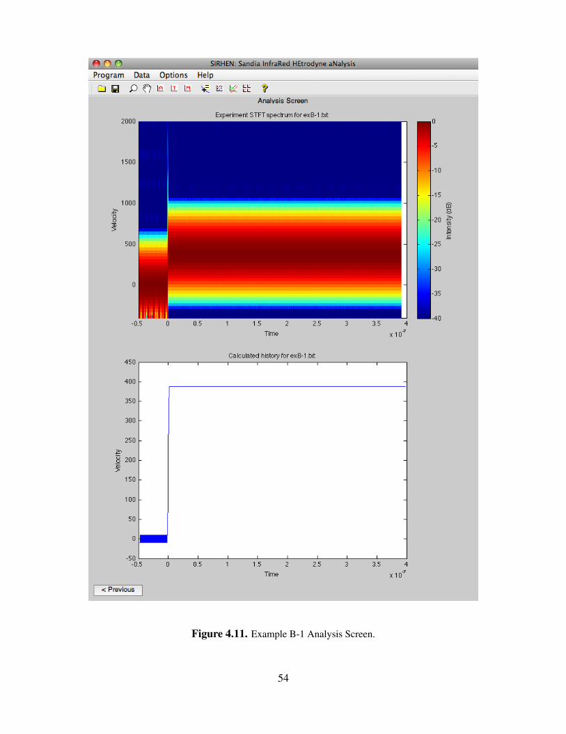
Figure 4.11. Example B-1 Analysis Screen.

54

(c)

(a) (b)

(d)

Figure 4.12. Example B-1 extracted velocities from peak findingmethods (solid lines) vs input velocity (dashed line): (a) maxi-mum, (b) centroid and robust, (c) parabola, and (d) Gaussian.

55

• Peak location method: maximum.

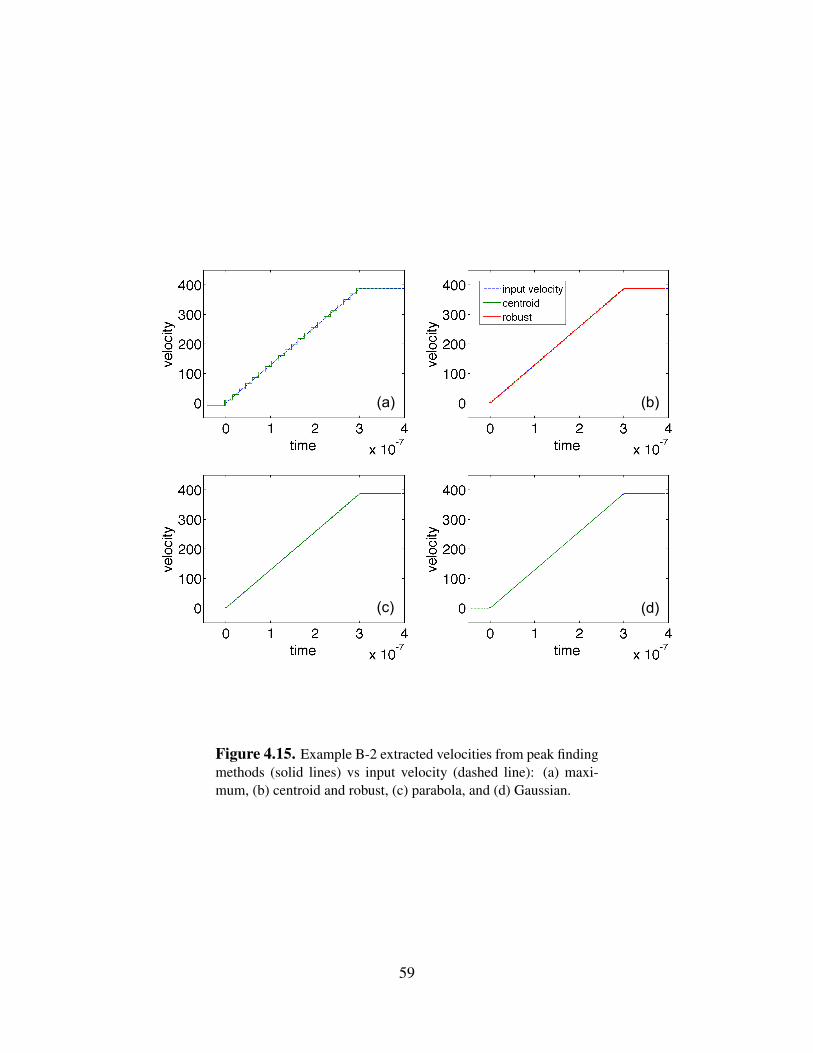
The Analysis Screen should now look like Fig. 4.14. Under the Data menu, select the Exporthistory action to save the extracted velocity profile. A comparison of the various peak findingmethods is shown in Fig. 4.15, where in each case only the “Peak location method” parameter waschanged. The maximum method gives a correct final velocity, but has an incorrect negative initialvelocity and discrete steps within the ramp profile. The centroid, robust, parabola, and Gaussianmethods all reduce the discreteness of the ramp profile, and have the correct initial zero velocity.Finally, the oscillations at the foot of the ramp observed in the earlier standard PDV example areeliminated in the frequency-conversion PDV example.

56

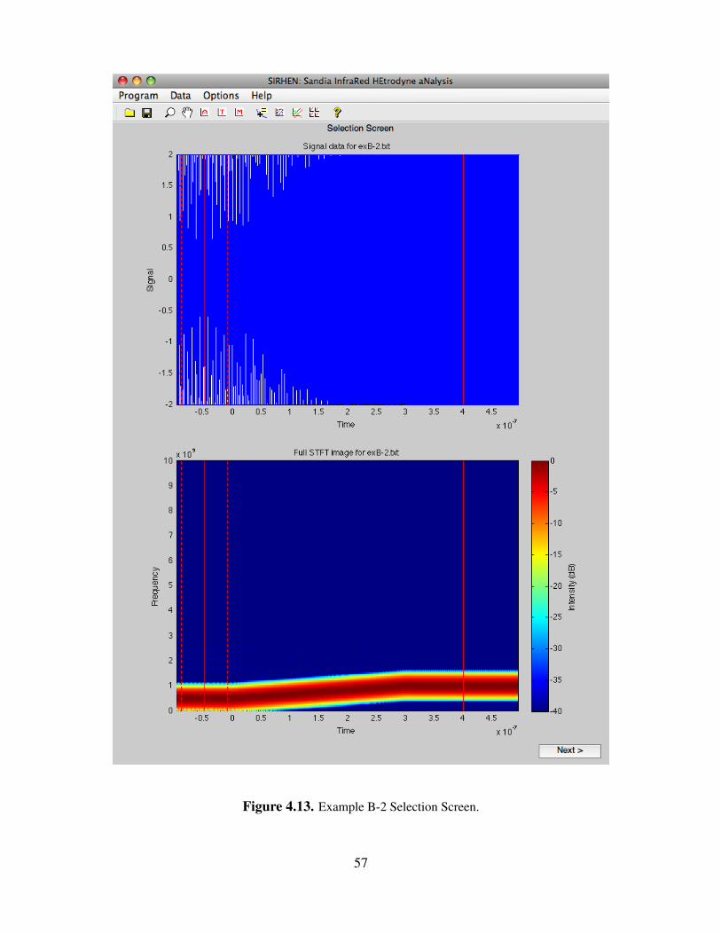
Figure 4.13. Example B-2 Selection Screen.

57

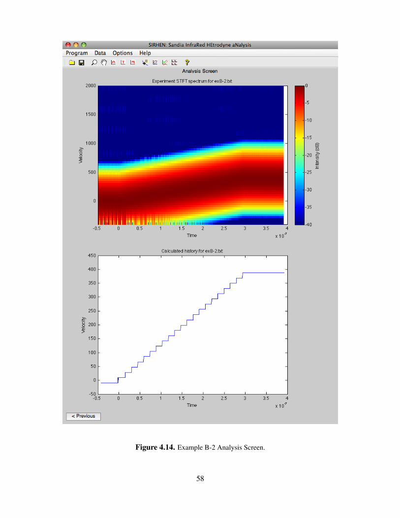
Figure 4.14. Example B-2 Analysis Screen.

58

(c)

(a) (b)

(d)

Figure 4.15. Example B-2 extracted velocities from peak findingmethods (solid lines) vs input velocity (dashed line): (a) maxi-mum, (b) centroid and robust, (c) parabola, and (d) Gaussian.

59

60

Chapter 5

Summary

5.1 Program features

The SIRHEN program reduces a photonic Doppler velocimetry (PDV) signal into a velocity his-tory. SIRHEN accepts a single data file in either text or binary format. Users may specify areference time range (over which an underlying beat frequency is characterized) and an experi-ment range (over which the analysis is performed). A short-time Fourier transform analysis is usedto generate the frequency spectrum of the PDV signal. The velocity history is extracted from thefrequency spectrum using a peak finding method. Data generated by SIRHEN can be exported toa text file for post-processing or saved in various graphical formats.

5.2 Future releases

Users should contact Tommy Ao (tao@sandia.gov) and/or Dan Dolan (dhdolan@sandia.gov) withquestions, bug reports, and feature requests. Bug fixes will be made as necessary and will bedistributed by email. No scheduled updates to SIRHEN is planned at this time, but new releaseswill be considered based on users’ feedback.

61

62

References

[1] L. M. Barker and R. E. Hollenbach, “Laser interferometer for measuring high velocities of anyreflecting surface,” Journal of Applied Physics, vol. 43, p. 4669, November 1972.

[2] C. F. McMillan, D. R. Goosman, N. L. Parker, L. L. Steinmetz, H. H. Chau, T. Huen, R. K.Whipkey, and S. J. Perry, “Velocimetry of fast surfaces using Fabry-Perot interferometry,”Review of Scientific Instruments, vol. 59, p. 1, 1988.

[3] O. T. Strand, D. R. Goosman, C. Martinez, and T. L. Whitworth, “Compact system for high-speed velocimetry using hetrodyne techniques,” Review of Scientific Instruments, vol. 77,p. 083108, August 2006.

[4] B. J. Jensen, D. B. Holtkamp, P. A. Rigg, and D. H. Dolan, “Accuracy limits and windowcorrections for photon Doppler velocimetry,” Journal of Applied Physics, vol. 101, p. 013523,August 2007.

[5] W. F. Hemsing, “Velocity sensing interferometer (VISAR) modification,” Review of ScientificInstruments, vol. 50, no. 1, pp. 73–78, 1979.

[6] D. H. Dolan, “THRIVE: a data reduction program for three-phase PDV/PDI and VISAR meau-rements,” Sandia report SAND2008-3871, Sandia National Laboratories, June 2008.

[7] A. V. Oppenheim and R. W. Schafer, Discrete-time signal processing. Prentice Hall, 1989.

[8] F. Harris, “On the use of windows for hamonic analysis with the discrete Fourier transform,”in Proceedings of the IEEE, vol. 66, pp. 51–83, IEEE, January 1978.

63

DISTRIBUTION:

1 MS 0425 S. C. Jones, 545

1 MS 0826 W. M. Trott, 1512

1 MS 0836 M. R. Baer, 1500

10 MS 1106 T. Ao, 1646

5 MS 1133 M. U. Anderson, 59165 MS 1133 J. Podsednik, 5916

1 MS 1157 K. J. Fleming, 54341

1 MS 1186 M. Herrmann, 1640

1 MS 1189 M. P. Desjarlais, 1640

1 MS 1193 R. G. Hacking, 165611 MS 1193 S. L. Payne, 16561

1 MS 1195 J. R. Asay, 16461 MS 1195 C. S. Alexander, 16461 MS 1195 J.-P. Davis, 16465 MS 1195 D. H. Dolan, 16461 MS 1195 D. G. Dalton, 16461 MS 1195 M. D. Furnish, 16461 MS 1195 R. J. Hickman, 16461 MS 1195 M. D. Knudson, 16461 MS 1195 B. V. Oliver, 16561 MS 1195 S. Root, 16461 MS 1195 W. D. Reinhart, 16461 MS 1195 J. L. Wise, 1646

1 MS 1205 C. A. Hall, 5902

1 MS 1454 M. D. Willis, 2552

1 MS 9042 T. J. Vogler, 8246

1 MS 0899 Technical Library, 9536 (electronic copy)

64