Embed Size (px)
Citation preview
Singular Solutions to the Monge-Ampere Equation
Connor Mooney
Submitted in partial fulfillment of the
requirements for the degree
of Doctor of Philosophy
in the Graduate School of Arts and Sciences
COLUMBIA UNIVERSITY
2015

c©2015
Connor Mooney
All Rights Reserved
ABSTRACT
Singular Solutions to the Monge-Ampere Equation
Connor Mooney
This thesis contains the author’s results on singular solutions to the Monge-Ampere equation
detD2u = 1.
We first prove that solutions are smooth away from a small closed singular set of Hausdorff n− 1
dimensional measure zero. We also construct solutions with a singular set of Hausdorff dimension
n− 1, showing that this result is optimal. As a consequence we obtain unique continuation for the
Monge-Ampere equation. Finally, we prove an interior W 2,1 estimate for singular solutions, and
we construct an example to show that this estimate is optimal.
Table of Contents
List of Figures iii
1 Introduction 1
1.1 Structure of the equation . . . . . . . . . . . . . . . . . . . . . . . . . . . . . . . . . 2
1.2 Previous results . . . . . . . . . . . . . . . . . . . . . . . . . . . . . . . . . . . . . . . 3
1.3 Singular solutions . . . . . . . . . . . . . . . . . . . . . . . . . . . . . . . . . . . . . . 4
1.4 Main results . . . . . . . . . . . . . . . . . . . . . . . . . . . . . . . . . . . . . . . . . 6
2 Examples 9
2.1 The Pogorelov example . . . . . . . . . . . . . . . . . . . . . . . . . . . . . . . . . . 9
2.2 Generalizations of the Pogorelov example . . . . . . . . . . . . . . . . . . . . . . . . 12
3 Preliminaries 18
3.1 Alexandrov solutions . . . . . . . . . . . . . . . . . . . . . . . . . . . . . . . . . . . . 18
3.2 General results on convex sets and functions . . . . . . . . . . . . . . . . . . . . . . . 19
3.3 Localization properties of sections . . . . . . . . . . . . . . . . . . . . . . . . . . . . 21
3.4 Previous results on singularities . . . . . . . . . . . . . . . . . . . . . . . . . . . . . . 23
4 Partial Regularity 26
4.1 Proof of Theorem 1.4.1 . . . . . . . . . . . . . . . . . . . . . . . . . . . . . . . . . . . 27
4.2 Example showing optimality of Theorem 1.4.1 . . . . . . . . . . . . . . . . . . . . . . 34
5 Unique Continuation 38
5.1 Unique continuation for linear equations . . . . . . . . . . . . . . . . . . . . . . . . . 38
i
5.2 Proof of Theorem 1.4.2 . . . . . . . . . . . . . . . . . . . . . . . . . . . . . . . . . . . 43
5.3 Counterexample . . . . . . . . . . . . . . . . . . . . . . . . . . . . . . . . . . . . . . 45
6 W 2,1 Estimate 49
6.1 W 2,1+ε estimate for strictly convex solutions . . . . . . . . . . . . . . . . . . . . . . . 50
6.2 W 2,1 regularity . . . . . . . . . . . . . . . . . . . . . . . . . . . . . . . . . . . . . . . 52
6.3 Proof of Theorem 1.4.3 . . . . . . . . . . . . . . . . . . . . . . . . . . . . . . . . . . . 54
6.4 Example showing optimality of Theorem 1.4.3 . . . . . . . . . . . . . . . . . . . . . . 68
Bibliography 72
ii
List of Figures
2.1 Graph of the Pogorelov solution restricted to a plane through the xn axis. . . . . . . 10
2.2 The image of the gradient map for solutions of the form u = rαf(xn). . . . . . . . . 12
2.3 Graph of a Lipschitz singular solution. . . . . . . . . . . . . . . . . . . . . . . . . . . 14
2.4 The image of the gradient map for solutions of the form u = r + rαf(xn). . . . . . . 15
4.1 The cone above xn = Chk generated by xk and the John ellipsoid of Svhk,0(0) has
a base containing a ball of radius at least (δ/2− C(a, δ)/Rk)h1/2k . . . . . . . . . . . . 32
4.2 ∇v(Brk(x)) contains an rk/2-neighborhood of the surface ∇v(Swk ), which projects in
the e1 direction (down) to a set of H2 measure at least cδ rk. . . . . . . . . . . . . . . 34
6.1 ∇v(Sk) contains an r/2-neighborhood of the surface ∇v(Sw(k+1/2)r), which projects
in the xn direction to a set of Hn−1 measure at least cγn/2−1. . . . . . . . . . . . . . 57
6.2 Swh (y) satisfies property F if the tangent plane at y, lifted by h, lies above h at 0. . . 59
6.3 . . . . . . . . . . . . . . . . . . . . . . . . . . . . . . . . . . . . . . . . . . . . . . . . 62
6.4 Lifting the tangent plane at y by h∗ = h + det(A)−2/nh we obtain a section of w
satisfying property F . . . . . . . . . . . . . . . . . . . . . . . . . . . . . . . . . . . . 63
6.5 For the case n = 3, the above figure implies that |Swh∗(y)| > ch∗/H. This, combined
with the volume estimate |Swh∗(y)| < C(h∗)3/2 and the upper bound on H from the
contradiction hypothesis give a lower bound of c| log h|−Cε for h∗. . . . . . . . . . . . 64
6.6 By convexity 2γ is at least h/H, giving a quantitative modulus of continuity for ∇w
near 0 which we exploit in Step 2 to obtain a contradiction. . . . . . . . . . . . . . . 65
6.7 ∇(u+|x|2/2)(Br(0)) contains an r/2-neighborhood of the surface∇(u+|x|2/2)(Swh (y)),
which projects in the xn direction to a set of Hn−1 measure at least crn−2| log r|(n−2)α1 . 67
iii
Acknowledgments
I would like to thank my thesis advisor Ovidiu Savin for his patient guidance and support. I
would also like to thank my previous teachers Simon Brendle and Leon Simon for their encourage-
ment. I am grateful to the analysis group at Columbia, especially Toti Daskalopoulos, Daniela De
Silva, and Yu Wang, for many helpful conversations. Finally, I would like to thank the mathemat-
ics department, especially Terrance Cope and Mary Young, for its hospitality, my friends Karsten
Gimre, Joao Guerreiro, Jordan Keller, Vivek Pal, Dan Rubin, and many others for making my stay
in New York so pleasant, Bogdan Apetri for many fun tennis games, and my parents for moral
support.
iv

to my parents
v
CHAPTER 1. INTRODUCTION
Chapter 1
Introduction
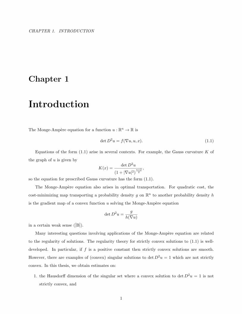
The Monge-Ampere equation for a function u : Rn → R is
detD2u = f(∇u, u, x). (1.1)
Equations of the form (1.1) arise in several contexts. For example, the Gauss curvature K of
the graph of u is given by
K(x) =detD2u
(1 + |∇u|2)n+2
2
,
so the equation for prescribed Gauss curvature has the form (1.1).
The Monge-Ampere equation also arises in optimal transportation. For quadratic cost, the
cost-minimizing map transporting a probability density g on Rn to another probability density h
is the gradient map of a convex function u solving the Monge-Ampere equation
detD2u =g
h(∇u)
in a certain weak sense ([B]).
Many interesting questions involving applications of the Monge-Ampere equation are related
to the regularity of solutions. The regularity theory for strictly convex solutions to (1.1) is well-
developed. In particular, if f is a positive constant then strictly convex solutions are smooth.
However, there are examples of (convex) singular solutions to detD2u = 1 which are not strictly
convex. In this thesis, we obtain estimates on:
1. the Hausdorff dimension of the singular set where a convex solution to detD2u = 1 is not
strictly convex, and
1
CHAPTER 1. INTRODUCTION
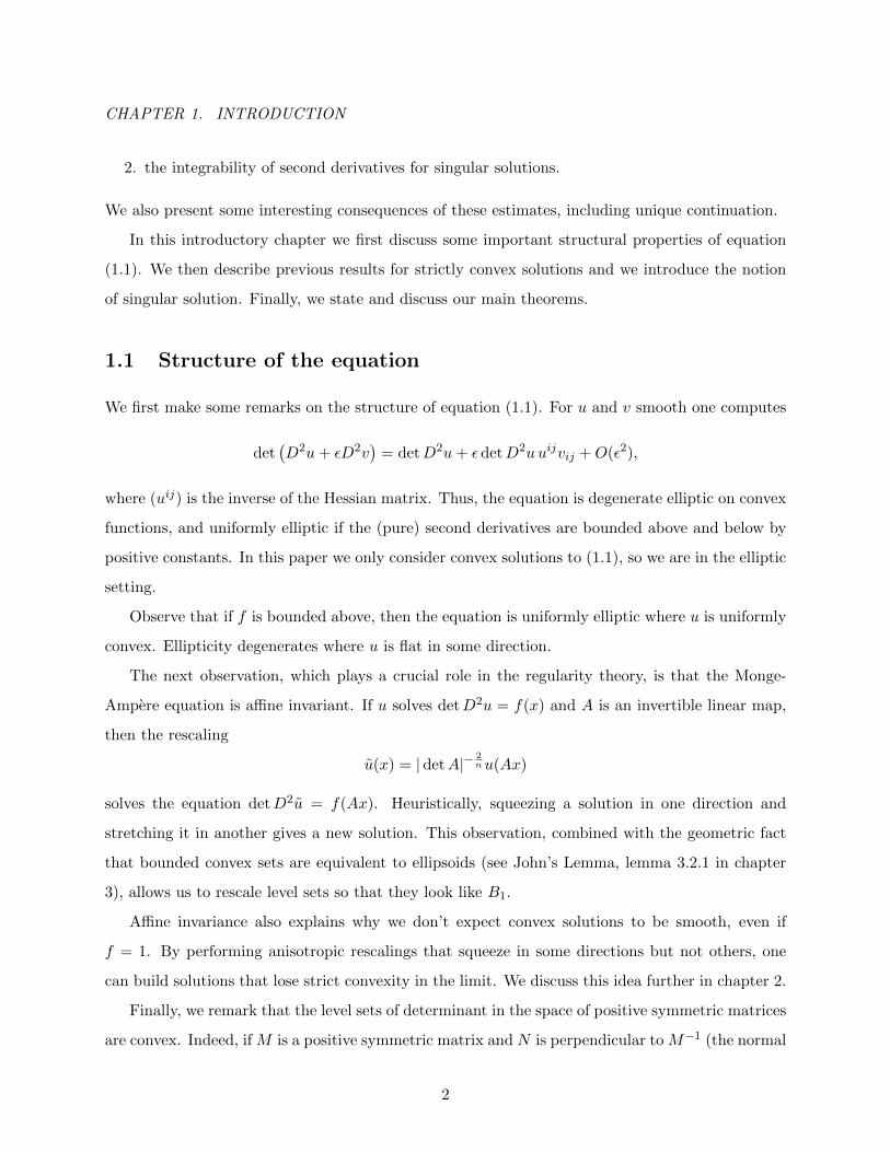
2. the integrability of second derivatives for singular solutions.
We also present some interesting consequences of these estimates, including unique continuation.
In this introductory chapter we first discuss some important structural properties of equation
(1.1). We then describe previous results for strictly convex solutions and we introduce the notion
of singular solution. Finally, we state and discuss our main theorems.
1.1 Structure of the equation
We first make some remarks on the structure of equation (1.1). For u and v smooth one computes
det(D2u+ εD2v
)= detD2u+ εdetD2uuijvij +O(ε2),
where (uij) is the inverse of the Hessian matrix. Thus, the equation is degenerate elliptic on convex
functions, and uniformly elliptic if the (pure) second derivatives are bounded above and below by
positive constants. In this paper we only consider convex solutions to (1.1), so we are in the elliptic
setting.
Observe that if f is bounded above, then the equation is uniformly elliptic where u is uniformly
convex. Ellipticity degenerates where u is flat in some direction.
The next observation, which plays a crucial role in the regularity theory, is that the Monge-
Ampere equation is affine invariant. If u solves detD2u = f(x) and A is an invertible linear map,
then the rescaling
u(x) = | detA|−2nu(Ax)
solves the equation detD2u = f(Ax). Heuristically, squeezing a solution in one direction and
stretching it in another gives a new solution. This observation, combined with the geometric fact
that bounded convex sets are equivalent to ellipsoids (see John’s Lemma, lemma 3.2.1 in chapter
3), allows us to rescale level sets so that they look like B1.
Affine invariance also explains why we don’t expect convex solutions to be smooth, even if
f = 1. By performing anisotropic rescalings that squeeze in some directions but not others, one
can build solutions that lose strict convexity in the limit. We discuss this idea further in chapter 2.
Finally, we remark that the level sets of determinant in the space of positive symmetric matrices
are convex. Indeed, if M is a positive symmetric matrix and N is perpendicular to M−1 (the normal
2
CHAPTER 1. INTRODUCTION
to the level set through M), then
det(M + εN) = detM − ε2 detMM ikM jlNijNkl +O(ε3).
Since M is positive the second term is negative. Thus, we can apply Evans-Krylov techniques to
the Monge-Ampere equation.
1.2 Previous results
Now we describe previous results on the regularity of solutions to detD2u = 1.
One consequence of the above observations is that if f = 1 and D2u > γI for some γ > 0, then
we have interior apriori estimates (in terms of γ) on all the derivatives. Indeed, using the equation
we see that the second derivatives of u are bounded above and below, so the equation is uniformly
elliptic. The Evans-Krylov theorem for concave uniformly elliptic equations (see e.g. [CC]) says
that the second derivatives are in fact continuous. (Actually, the first result in this direction is due
to Calabi ([Cal]), see remark 1.2.1). By Schauder theory we have second derivative estimates for
the linearized equation, and we can bootstrap to get estimates for all derivatives.
Remark 1.2.1. Using the equation more carefully, Calabi ([Cal]) obtained an estimate on the third
derivatives at a point in terms of the maximum of the second derivates in a neighborhood of
this point. Thus, once the second derivatives are bounded, they are Lipschitz. Interestingly, in
dimensions five or smaller, Calabi’s techniques control the third derivatives at a point in terms of
the second derivatives at that point. This gives a Liouville theorem (global solutions to detD2u = 1
are paraboloids) in dimensions five or smaller which doesn’t rely on a C2 estimate.
Thus, the regularity problem for f = 1 is reduced to the problem of bounding the second
derivatives. The key result in this direction, due to Pogorelov ([P]), bounds D2u above on a level
set of u in terms of the geometry of the approximating ellipsoid of this level set, and the maximum
of |∇u| on this set. The idea is that by the concavity of the equation, the pure second derivatives
uee are subsolutions to the linearized equation and thus cannot have local maxima. Pogorelov
applies the maximum principle to the quantity
log(uee) + log |u|+ 1
2u2e
on the zero level set. The second term acts as a cutoff function.
3
CHAPTER 1. INTRODUCTION
Remark 1.2.2. Pogorelov’s estimate roughly says that we can control all the derivatives of a solution
to detD2u = 1 on the interior of a domain Ω ⊂ Rn in terms of a modulus of strict convexity for
the solution. Indeed, if u is strictly convex then any supporting plane that touches u on the
interior lies strictly below the boundary data, so we can lift it a little to carve out a level set (up
to subtracting a linear function) whose geometry depends only on the modulus of convexity of
u. However, Pogorelov’s estimate requires the solution to be C4 apriori since we differentiate the
equation twice.
This statement was not made rigorous until Caffarelli, Nirenberg and Spruck ([CNS]) solved the
Dirichlet problem on uniformly convex domains with C3 boundary and C3 boundary data. They
accomplish this by obtaining apriori C2,α estimates up to the boundary and using the method
of continuity. Interior regularity for any strictly convex solution follows by solving the Dirichlet
problem on smooth approximations to level sets and using the interior derivative estimates.
Remark 1.2.3. One actually needs C3 boundary and boundary data to get second derivative es-
timates up to the boundary. The idea is to use the cubic expansion to show that the tangential
second derivatives at a boundary point are strictly positive. Combining this with the equation, one
obtains bounds on all the second derivatives up to the boundary.
To show necessity, look for a solution u(x, y) on y > x2 with the homogeneity
u(x, y) =1
λ3u(λx, λ2y),
which has C2,1 boundary data growing cubically in the tangential directions at 0. Letting
u(t, 1) = f(t)
we have u(x, y) = y3/2f(xy−1/2
), and we get the example if f solves the ODE
(3f + tf ′)f ′′ − f ′2 = 4.
1.3 Singular solutions
We now discuss the notion of singular solution. Pogorelov showed by example that solutions to
detD2u = 1 are not always strictly convex ([P]). Write x = (x′, xn). The Pogorelov solution has
the form
u(x′, xn) = |x′|2−2/nf(xn), n ≥ 3,
4
CHAPTER 1. INTRODUCTION
and it solves detD2u = 1 in |xn| < ρ for some small ρ. We will discuss the Pogorelov example
and more complicated constructions in detail in chapter 2. For now we highlight the important
features.
First, one way to motivate this example comes from affine invariance. It is invariant under
cylindrical rescalings:
u(x′, xn) =1
λ2−2/nu(λx′, xn).
One can think of u as the rescaling limit of some classical solution in the slab |xn| < ρ. There
are similar solutions, due to Caffarelli ([C3]), which are invariant under transformations preserving
subspaces of any dimension strictly less than n2 . We discuss these examples in chapter 2.
Remark 1.3.1. Caffarelli also shows in [C3] that the agreement set between a solution to detD2u = 1
and a tangent plane has dimension strictly less than n2 , so his examples are optimal. We give a
short new proof of this result (see lemma 3.4.4) in chapter 3. This implies in particular that in two
dimensions, solutions are strictly convex, hence smooth. The strict convexity of solutions in two
dimensions is a classical result (see e.g. [Al]).
Second, this example agrees with its tangent plane on the xn axis. If a supporting plane agrees
with a solution at more than one point, we call the agreement set a “singularity,” and we say that
the solution is a “singular solution.” The Pogorelov solution has a singularity along the xn axis. It
is smooth away from the singularity and C1,1−2/n in |xn| < ρ, and as we approach the xn axis the
radial (x′) second derivatives blow up while the second derivatives in the en direction go to zero.
Singular solutions cannot be classical because at any point on a singularity, one of the pure
second derivatives would be zero. However, singular solutions are weak solutions in for example
the viscosity and Alexandrov senses (see chapter 3 for a precise definition).
Finally, an important observation is that this example is not global (it is only defined in
|xn| < ρ) and the singularity extends to the boundary. Caffarelli ([C1]) showed that the (convex)
agreement set between a solution to 0 < λ ≤ detD2u ≤ 1λ and a tangent plane has no interior
extremal points; if it is not a single point, then it must extend to the boundary, and it has only
“flat edges” in the interior. This observation, along with affine invariance, allows one to control
the geometry of level sets. It facilitated the proof of a C1,α estimate for strictly convex solutions to
λ ≤ detD2u ≤ 1λ , and gave a modulus of strict convexity when the boundary data are C1,β for any
5
CHAPTER 1. INTRODUCTION
β > 1 − 2/n. In light of the Pogorelov example, this gave a more or less optimal characterization
of when solutions to detD2u = 1 are strictly convex, hence smooth.
Remark 1.3.2. Caffarelli’s results also allowed the extension of perturbation results and covering ar-
guments from uniformly elliptic theory to strictly convex solutions to the Monge-Ampere equation.
In particular, he obtained interior C2,α estimates when the right side is Cα, and W 2,p estimates
when the right side has small oscillation depending on p ([C2]).
1.4 Main results
The above results give context to the work in this thesis, which gives estimates for singular solutions
to detD2u = 1 which are not strictly convex.
Since there are many examples of singular solutions (see chapter 2), a natural problem is to
find the largest possible Hausdorff dimension of the singular set. Our first theorem addresses this
problem. We say a convex function u is strictly convex at x0 if there exists a supporting plane L
such that
u = L = x0.
Our first theorem is:
Theorem 1.4.1. Assume u is an Alexandrov solution to
detD2u ≥ 1
in B1 ⊂ Rn. Then u is strictly convex away from a singular set Σ with
Hn−1(Σ) = 0.
We also construct examples of solutions to detD2u = 1 with a singular set of Hausdorff dimen-
sion as close as we like to n− 1, which shows that this estimate is optimal.
By the previous discussion, this theorem implies that solutions to detD2u = 1 are smooth away
from a closed singular set of Hausdorff n− 1 dimensional measure zero.
The key new idea is to show that u separates from its tangent plane much faster than quadrat-
ically in at least two directions perpendicular to a singular line. We do this by examining the
geometry of level sets of u+ |x|2 near points in Σ.
6
CHAPTER 1. INTRODUCTION
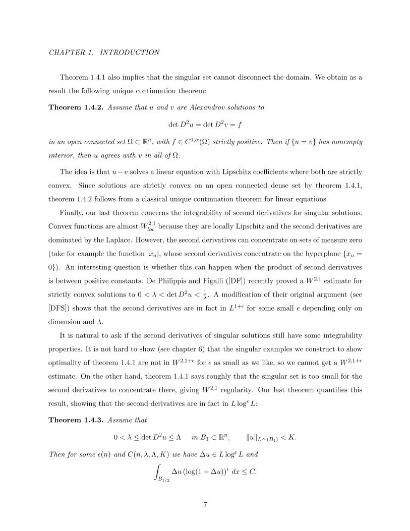
Theorem 1.4.1 also implies that the singular set cannot disconnect the domain. We obtain as a
result the following unique continuation theorem:
Theorem 1.4.2. Assume that u and v are Alexandrov solutions to
detD2u = detD2v = f
in an open connected set Ω ⊂ Rn, with f ∈ C1,α(Ω) strictly positive. Then if u = v has nonempty
interior, then u agrees with v in all of Ω.
The idea is that u−v solves a linear equation with Lipschitz coefficients where both are strictly
convex. Since solutions are strictly convex on an open connected dense set by theorem 1.4.1,
theorem 1.4.2 follows from a classical unique continuation theorem for linear equations.
Finally, our last theorem concerns the integrability of second derivatives for singular solutions.
Convex functions are almost W 2,1loc because they are locally Lipschitz and the second derivatives are
dominated by the Laplace. However, the second derivatives can concentrate on sets of measure zero
(take for example the function |xn|, whose second derivatives concentrate on the hyperplane xn =
0). An interesting question is whether this can happen when the product of second derivatives
is between positive constants. De Philippis and Figalli ([DF]) recently proved a W 2,1 estimate for
strictly convex solutions to 0 < λ < detD2u < 1λ . A modification of their original argument (see
[DFS]) shows that the second derivatives are in fact in L1+ε for some small ε depending only on
dimension and λ.
It is natural to ask if the second derivatives of singular solutions still have some integrability
properties. It is not hard to show (see chapter 6) that the singular examples we construct to show
optimality of theorem 1.4.1 are not in W 2,1+ε for ε as small as we like, so we cannot get a W 2,1+ε
estimate. On the other hand, theorem 1.4.1 says roughly that the singular set is too small for the
second derivatives to concentrate there, giving W 2,1 regularity. Our last theorem quantifies this
result, showing that the second derivatives are in fact in L logε L:
Theorem 1.4.3. Assume that
0 < λ ≤ detD2u ≤ Λ in B1 ⊂ Rn, ‖u‖L∞(B1) < K.
Then for some ε(n) and C(n, λ,Λ,K) we have ∆u ∈ L logε L and∫B1/2
∆u (log(1 + ∆u))ε dx ≤ C.
7
CHAPTER 1. INTRODUCTION
The key idea is to refine our techniques from theorem 1.4.1 to show that u separates from its
tangent plane logarithmically faster than quadratic in at least two directions perpendicular to a
singular line. We also construct a singular solution to detD2u = 1 whose second derivatives are
not in L logM L for some M , showing that theorem 1.4.3 is almost optimal.
Remark 1.4.4. All of our three main theorems are new even in the case f = 1. The difficulties
of the proofs come from the degeneracy of level sets near singularities. The hypotheses on f in
theorems 1.4.2 and 1.4.3 are simply those required to apply the appropriate regularity results for
strictly convex solutions away from the singular set.
The paper is organized as follows. In chapter 2 we present some important examples of singular
solutions to detD2u = 1. These include the well-known Pogorelov example and some general-
izations. In chapter 3 we prove some results from convex analysis and use them to prove useful
localization properties of level sets. We also prove some previous results on the geometry of singu-
larities. In chapter 4 we use the results from chapter 3 to prove theorem 1.4.1, and we construct
solutions to detD2u = 1 with singular sets of Hausdorff dimension as close as we like to n − 1,
showing that theorem 1.4.1 is optimal. In chapter 5 we prove theorem 1.4.2 by applying a classi-
cal unique continuation theorem in the set of strict convexity. We also discuss the linear theory.
Finally, in chapter 6 we prove theorem 1.4.3 and we construct a singular example showing it is
optimal.
8
CHAPTER 2. EXAMPLES
Chapter 2
Examples
In this chapter we present some instructive examples of singular solutions to detD2u = 1. We begin
by closely examining the well-known example of Pogorelov. We then discuss more complicated
examples, which are constructed in a similar way.
2.1 The Pogorelov example
Harmonic functions on some domain are smooth in the interior even if the boundary data are
irregular. In contrast, we do not expect a purely local regularity theory for the Monge-Ampere
equation due to affine invariance. Indeed, if we have a smooth solution to
detD2u = 1
in |xn| < 1 then the anisotropic rescaling
uλ(x′, xn) =1
λ2−2/nu(λx′, xn)
is also a solution. As λ gets large, the second derivatives in the x′ directions blow up on the xn-axis,
and we lose strict convexity there.
To construct the well-known Pogorelov solution one searches for functions that are invariant
under this rescaling:
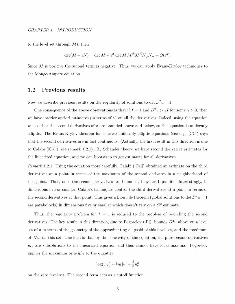
u(x′, xn) = |x′|2−2/nf(xn), n ≥ 3.
9
CHAPTER 2. EXAMPLES
¿x ' ¿=0
| x ' |=0
u ( x ' , xn)
rr 2−2/n
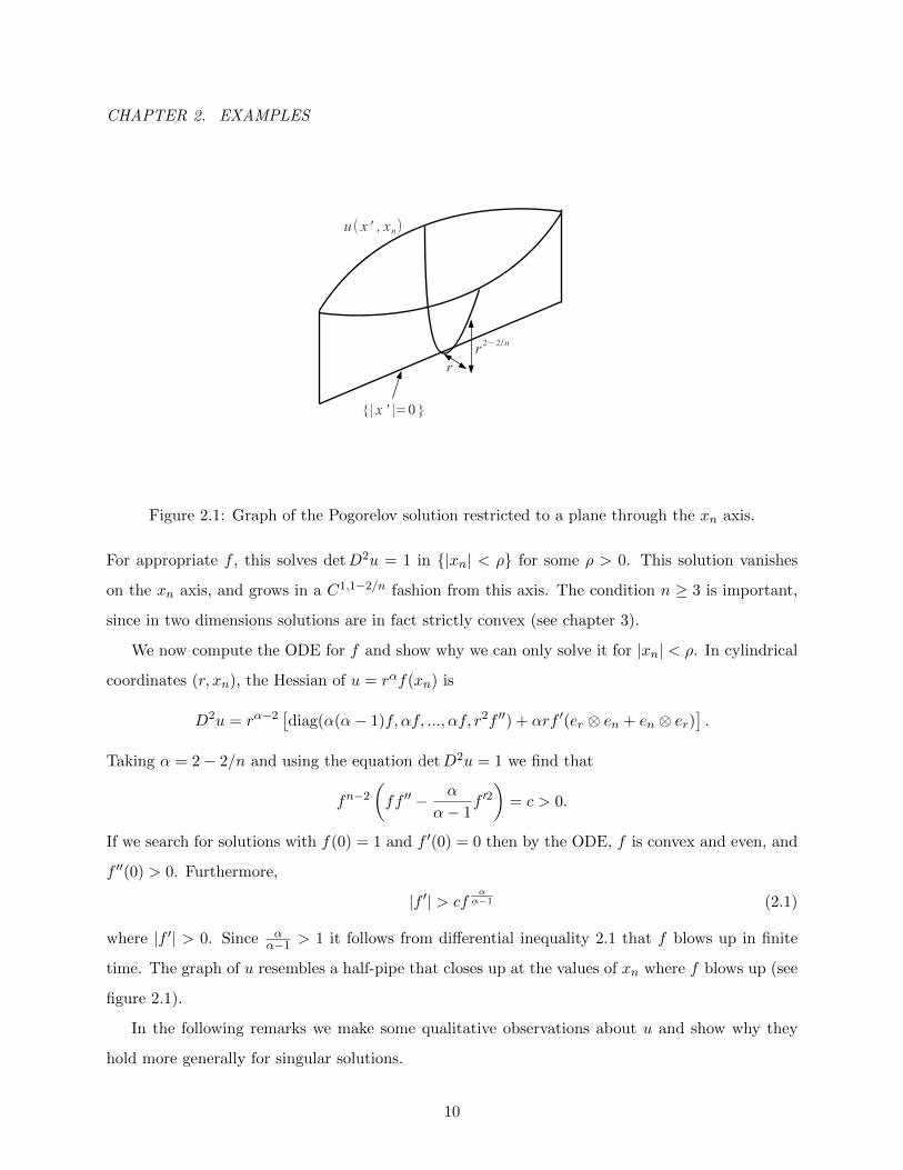
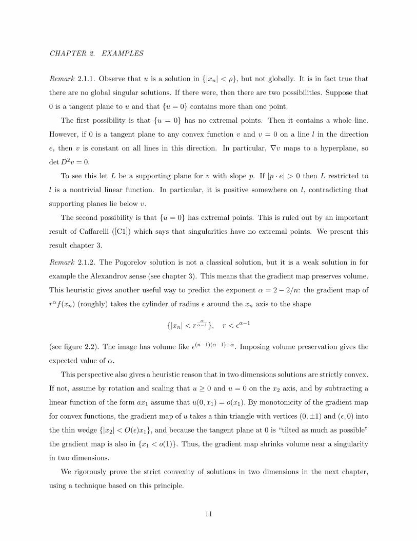
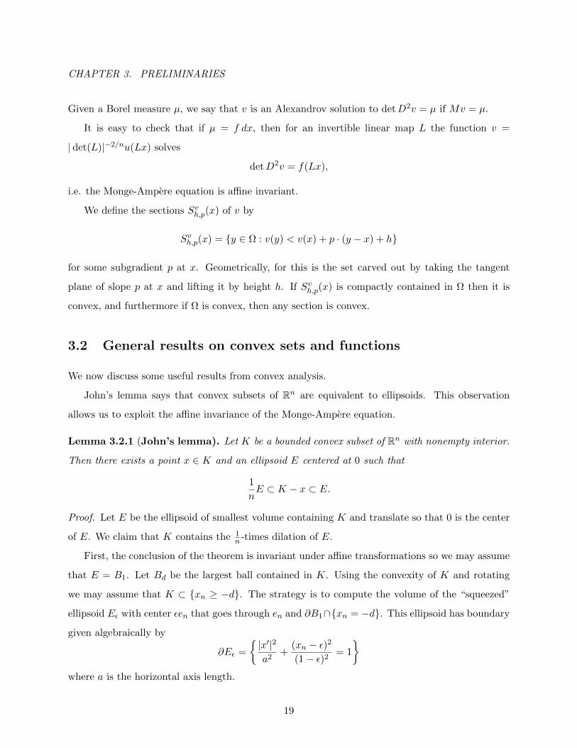
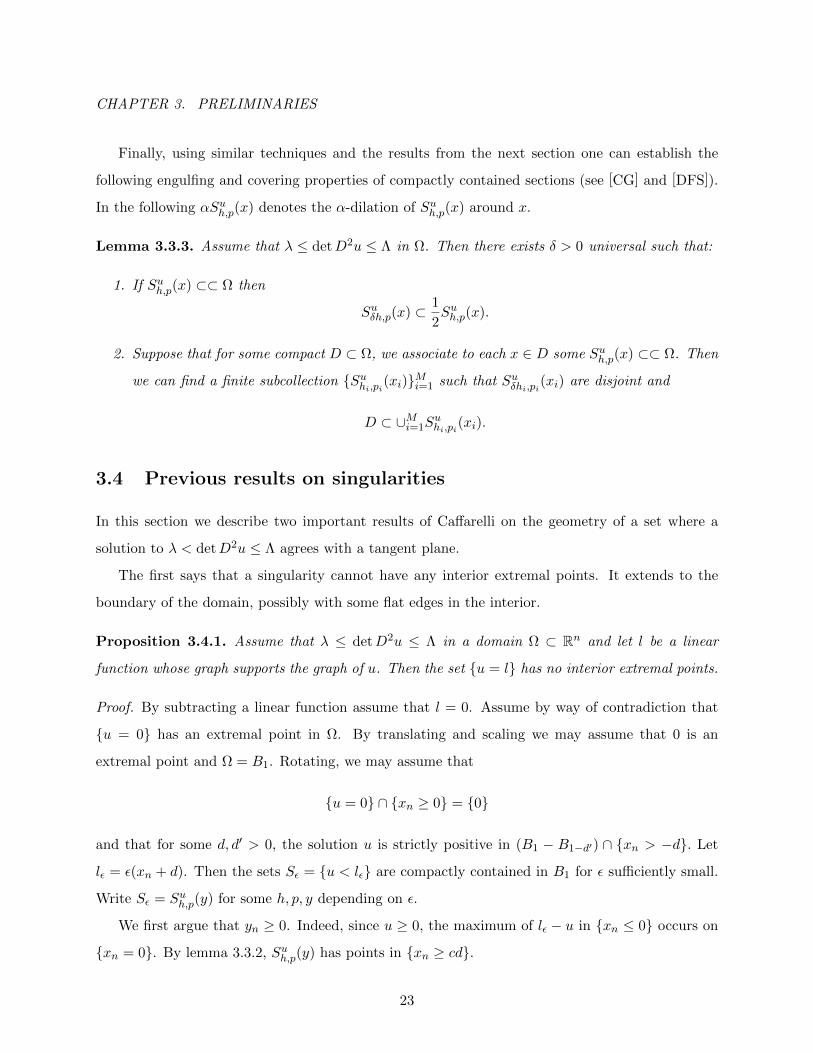
Figure 2.1: Graph of the Pogorelov solution restricted to a plane through the xn axis.
For appropriate f , this solves detD2u = 1 in |xn| < ρ for some ρ > 0. This solution vanishes
on the xn axis, and grows in a C1,1−2/n fashion from this axis. The condition n ≥ 3 is important,
since in two dimensions solutions are in fact strictly convex (see chapter 3).
We now compute the ODE for f and show why we can only solve it for |xn| < ρ. In cylindrical
coordinates (r, xn), the Hessian of u = rαf(xn) is
D2u = rα−2[diag(α(α− 1)f, αf, ..., αf, r2f ′′) + αrf ′(er ⊗ en + en ⊗ er)
].
Taking α = 2− 2/n and using the equation detD2u = 1 we find that
fn−2
(ff ′′ − α
α− 1f ′2)
= c > 0.
If we search for solutions with f(0) = 1 and f ′(0) = 0 then by the ODE, f is convex and even, and
f ′′(0) > 0. Furthermore,
|f ′| > cfαα−1 (2.1)
where |f ′| > 0. Since αα−1 > 1 it follows from differential inequality 2.1 that f blows up in finite
time. The graph of u resembles a half-pipe that closes up at the values of xn where f blows up (see
figure 2.1).
In the following remarks we make some qualitative observations about u and show why they
hold more generally for singular solutions.
10
CHAPTER 2. EXAMPLES
Remark 2.1.1. Observe that u is a solution in |xn| < ρ, but not globally. It is in fact true that
there are no global singular solutions. If there were, then there are two possibilities. Suppose that
0 is a tangent plane to u and that u = 0 contains more than one point.
The first possibility is that u = 0 has no extremal points. Then it contains a whole line.
However, if 0 is a tangent plane to any convex function v and v = 0 on a line l in the direction
e, then v is constant on all lines in this direction. In particular, ∇v maps to a hyperplane, so
detD2v = 0.
To see this let L be a supporting plane for v with slope p. If |p · e| > 0 then L restricted to
l is a nontrivial linear function. In particular, it is positive somewhere on l, contradicting that
supporting planes lie below v.
The second possibility is that u = 0 has extremal points. This is ruled out by an important
result of Caffarelli ([C1]) which says that singularities have no extremal points. We present this
result chapter 3.
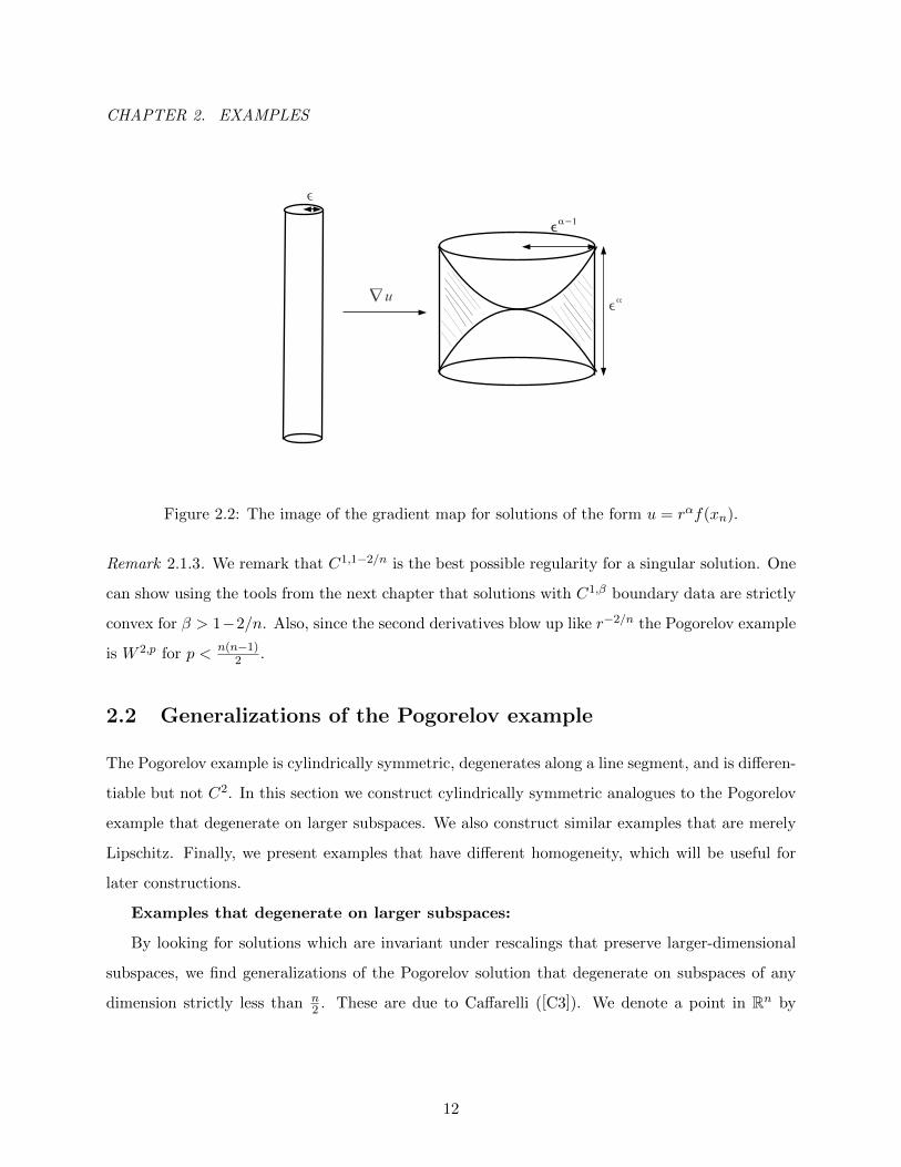
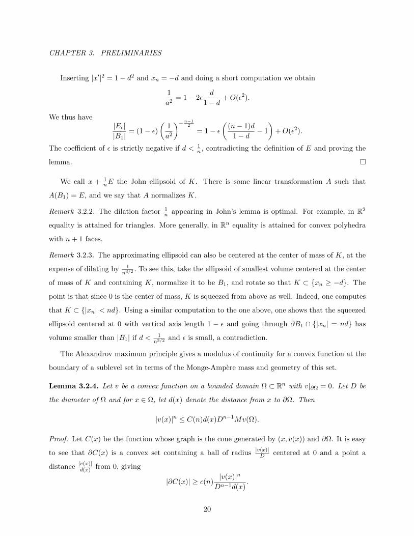
Remark 2.1.2. The Pogorelov solution is not a classical solution, but it is a weak solution in for
example the Alexandrov sense (see chapter 3). This means that the gradient map preserves volume.
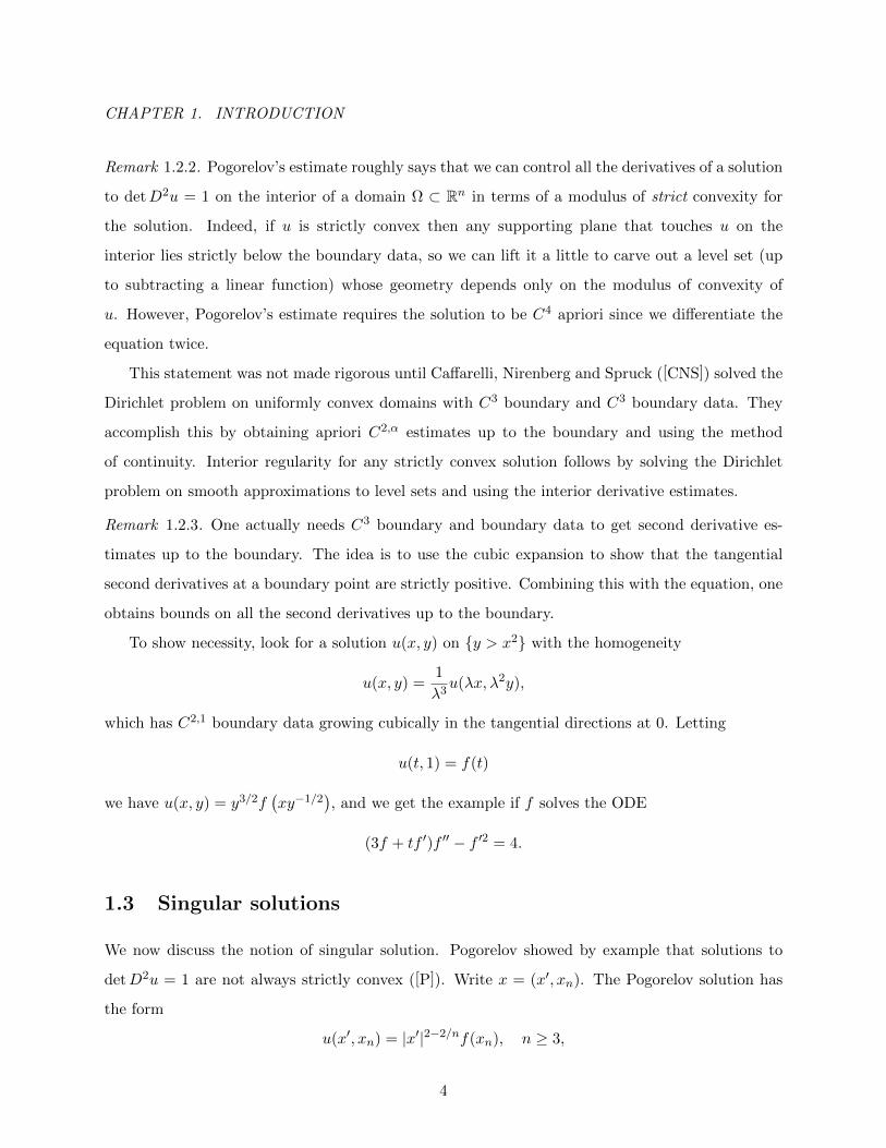
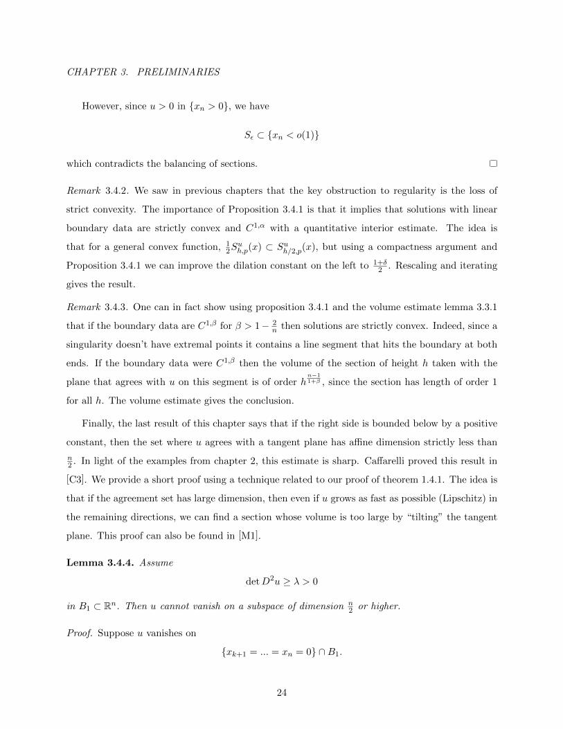
This heuristic gives another useful way to predict the exponent α = 2− 2/n: the gradient map of
rαf(xn) (roughly) takes the cylinder of radius ε around the xn axis to the shape
|xn| < rαα−1 , r < εα−1
(see figure 2.2). The image has volume like ε(n−1)(α−1)+α. Imposing volume preservation gives the
expected value of α.
This perspective also gives a heuristic reason that in two dimensions solutions are strictly convex.
If not, assume by rotation and scaling that u ≥ 0 and u = 0 on the x2 axis, and by subtracting a
linear function of the form ax1 assume that u(0, x1) = o(x1). By monotonicity of the gradient map
for convex functions, the gradient map of u takes a thin triangle with vertices (0,±1) and (ε, 0) into
the thin wedge |x2| < O(ε)x1, and because the tangent plane at 0 is “tilted as much as possible”
the gradient map is also in x1 < o(1). Thus, the gradient map shrinks volume near a singularity
in two dimensions.
We rigorously prove the strict convexity of solutions in two dimensions in the next chapter,
using a technique based on this principle.
11
CHAPTER 2. EXAMPLES
ϵ
∇ u
ϵα−1ϵα−1
ϵα
Figure 2.2: The image of the gradient map for solutions of the form u = rαf(xn).
Remark 2.1.3. We remark that C1,1−2/n is the best possible regularity for a singular solution. One
can show using the tools from the next chapter that solutions with C1,β boundary data are strictly
convex for β > 1−2/n. Also, since the second derivatives blow up like r−2/n the Pogorelov example
is W 2,p for p < n(n−1)2 .
2.2 Generalizations of the Pogorelov example
The Pogorelov example is cylindrically symmetric, degenerates along a line segment, and is differen-
tiable but not C2. In this section we construct cylindrically symmetric analogues to the Pogorelov
example that degenerate on larger subspaces. We also construct similar examples that are merely
Lipschitz. Finally, we present examples that have different homogeneity, which will be useful for
later constructions.
Examples that degenerate on larger subspaces:
By looking for solutions which are invariant under rescalings that preserve larger-dimensional
subspaces, we find generalizations of the Pogorelov solution that degenerate on subspaces of any
dimension strictly less than n2 . These are due to Caffarelli ([C3]). We denote a point in Rn by
12
CHAPTER 2. EXAMPLES
(x, y) with x ∈ Rn−k and y ∈ Rk, and we write r = |x|, t = |y|. These solutions have the form
u(x, y) = r2− 2kn f(t), n ≥ 3, k <
n
2.
Let α = 2− 2kn . In these coordinates the Hessian is
D2u = rα−2
α(α− 1)f 0 · · · 0 0 · · · 0 αrf ′
0 αf 0 · · · 0 0 · · · 0
0 0 · · · αf 0 0 · · · 0
0 0 · · · 0 r2
t f′ 0 0 0
0 0 · · · 0 0 · · · · · · 0
0 0 · · · 0 · · · · · · r2
t f′ · · ·
αrf ′ 0 · · · 0 0 · · · 0 r2f ′′
.
One computes
detD2u = cfn−k−1f ′k−1
tk−1
(ff ′′ − α
α− 1f ′2).
Taking for example f(t) = 1 + t2 we can produce a solution with smooth right hand side bounded
between two positive constants for t bounded.
Remark 2.2.1. These solutions vanish on subspaces of dimension k for any k < n2 . They are C1, 1− 2k
n ,
and W 2,p for p < n(n−k)2k . In [C3] Caffarelli shows this dimension is optimal. We give a new proof
(see also [M1]) in the next chapter.
Remark 2.2.2. It is not hard to build solutions which vanish on subspaces of dimension k with
k < n2 and right hand side exactly 1. Let w be the solution constructed above, multiplied by a
large constant so that detD2w > 1 in the cylinder Q = r < 1, t < 1. Then solve the Dirichlet
problem (see e.g. [Gut])
detD2u = 1, u|∂Q = w.
Since w is a subsolution we have w ≤ u. It follows that u ≥ 0 when r = 0. On the other hand, u = 0
on ∂Q ∩ r = 0, so by convexity u vanishes when r = 0. This shows explicitly that solutions to
the Monge-Ampere equation can have singularities that “propagate from boundary irregularities,”
unlike harmonic functions which become smooth as soon as we step away from the boundary.
Lipschitz examples:
13
CHAPTER 2. EXAMPLES
¿x ' ¿=0
| x ' |=0
u ( x ' , xn)
r
r n /2
| x ' |
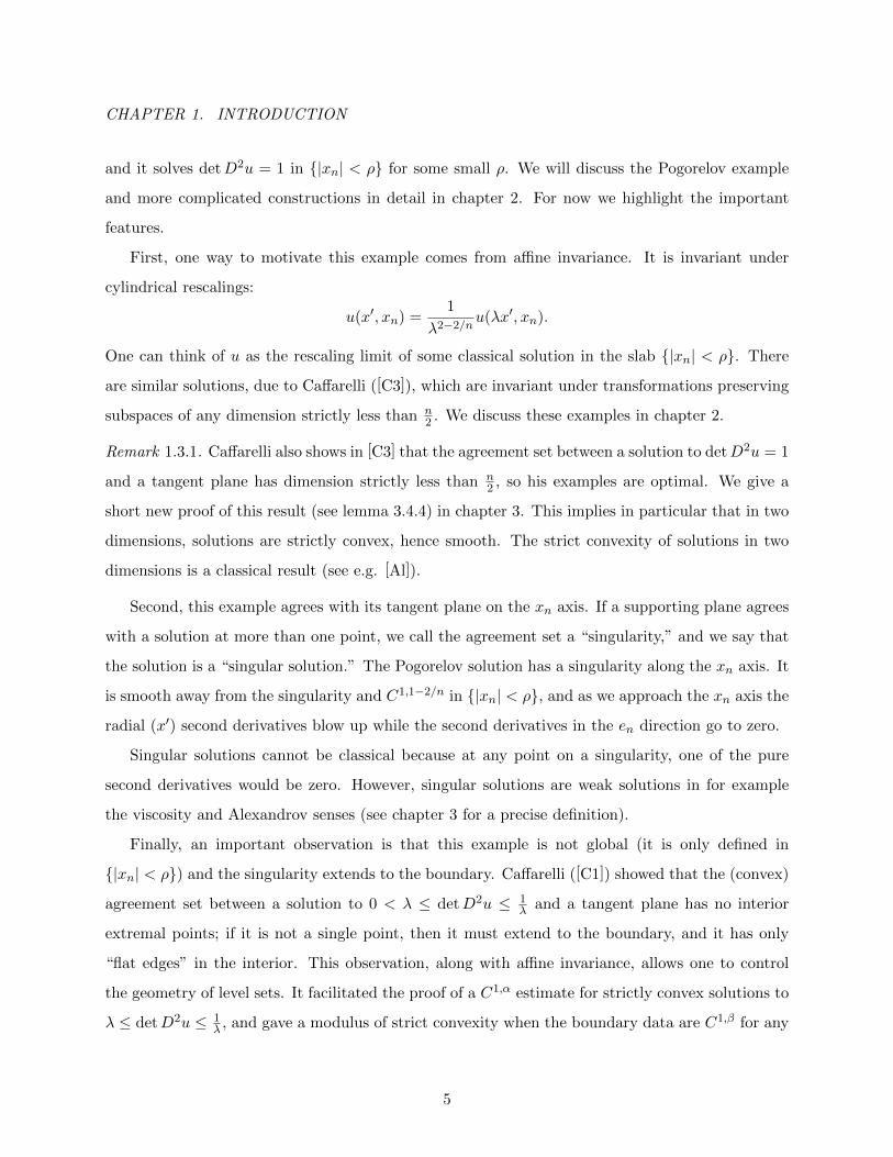
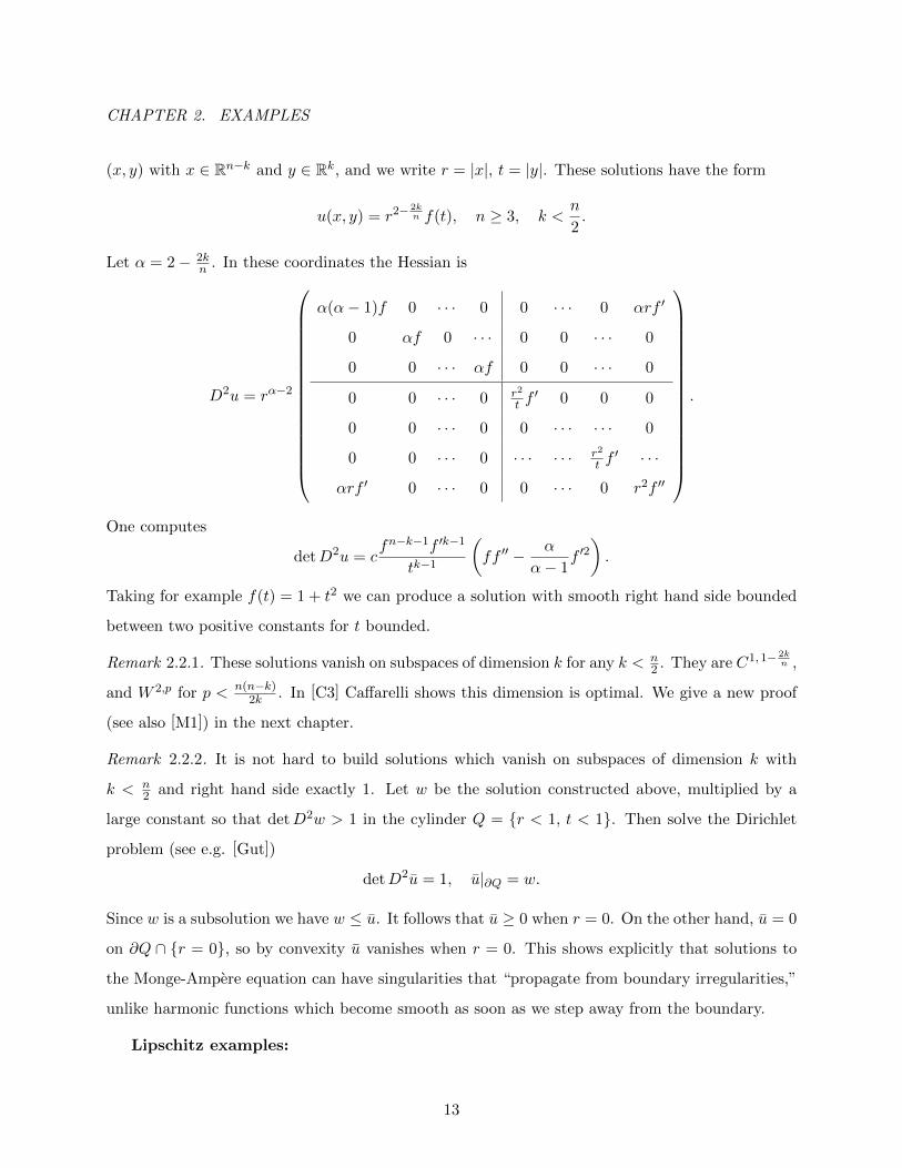
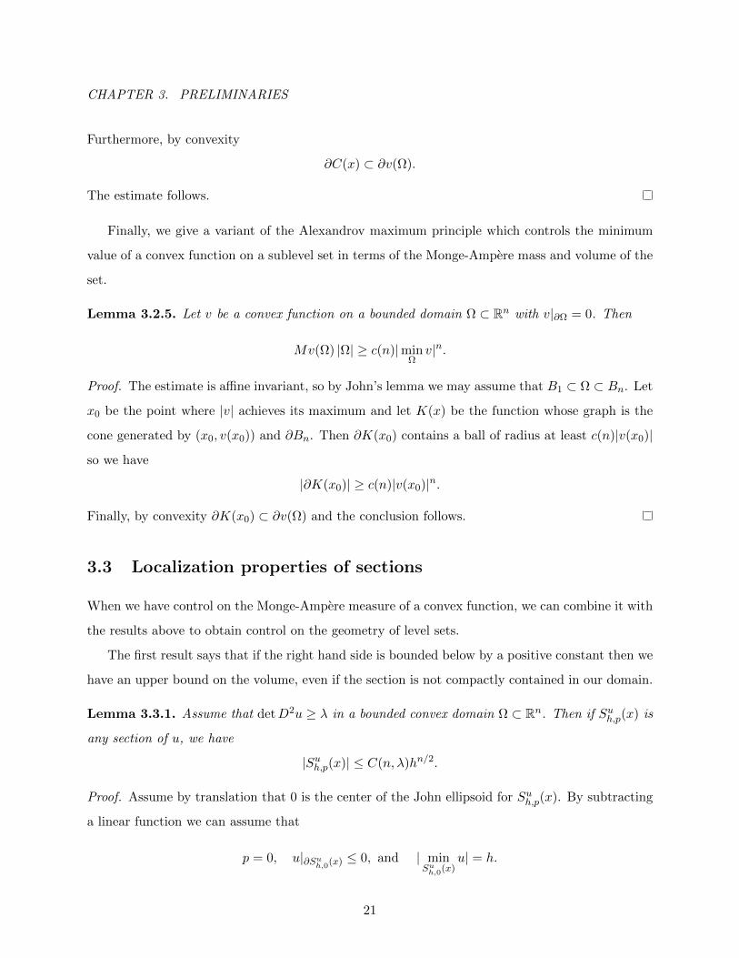
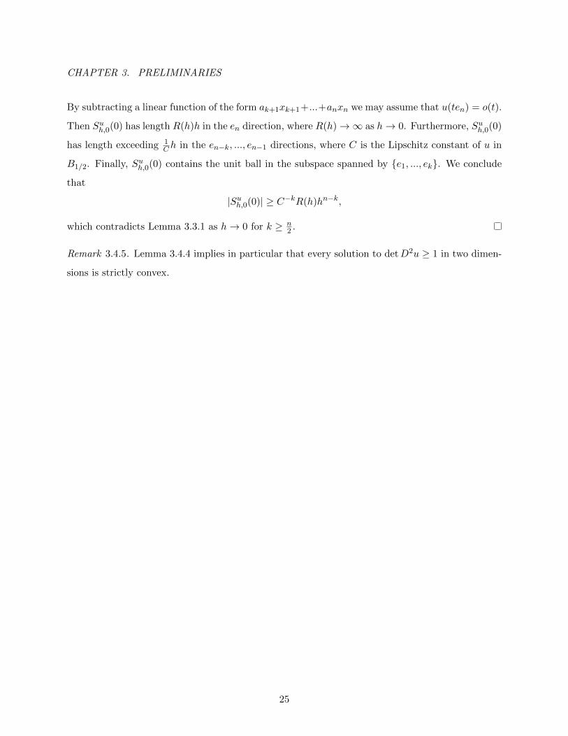
Figure 2.3: Graph of a Lipschitz singular solution.
The examples presented so far are differentiable. We now present a singular solution which is
merely Lipschitz, the least possible regularity for a convex function. For x = (x′, xn) with |x′| = r
and xn = t it has the form
u(x′, xn) = r + rn2 g(t), n ≥ 3.
Let α = n2 . The Hessian is
D2u =1
rdiag
(α(α− 1)rα−1g, 1 + αrα−1g, ..., 1 + αrα−1g, rα+1g′′
)+ αrα−1g′(er ⊗ en + en ⊗ er).
One computes
detD2u = c(1 + αrα−1g)n−2
(gg′′ − α
α− 1g′2),
so we get solutions in B1 to an equation with right hand side bounded between two positive
constants. The graphs of these solutions are tangent to the graph of |x′| on the xn axis, and
separate from |x′| like rn/2 (see figure 2.3).
Remark 2.2.3. Again, when we solve the Dirichlet problem with constant right side and the same
boundary data as u, the solution “inherits” the Lipschitz singularity of u.
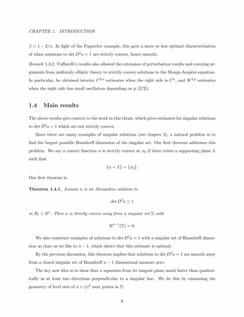
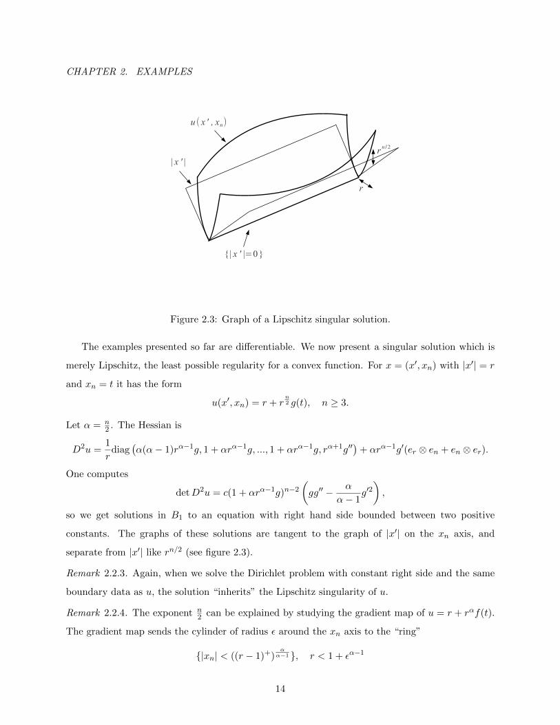
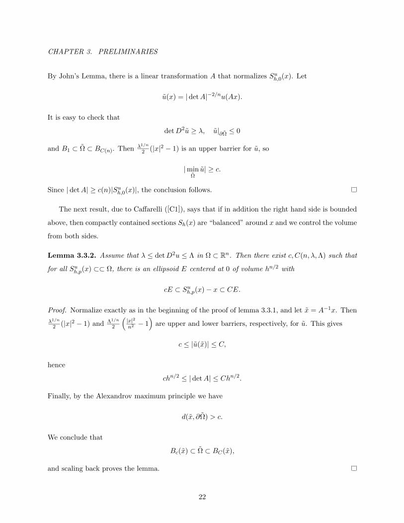
Remark 2.2.4. The exponent n2 can be explained by studying the gradient map of u = r + rαf(t).
The gradient map sends the cylinder of radius ε around the xn axis to the “ring”
|xn| < ((r − 1)+)αα−1 , r < 1 + εα−1
14
CHAPTER 2. EXAMPLES
ϵ
∇ u
ϵα−1
ϵα
Figure 2.4: The image of the gradient map for solutions of the form u = r + rαf(xn).
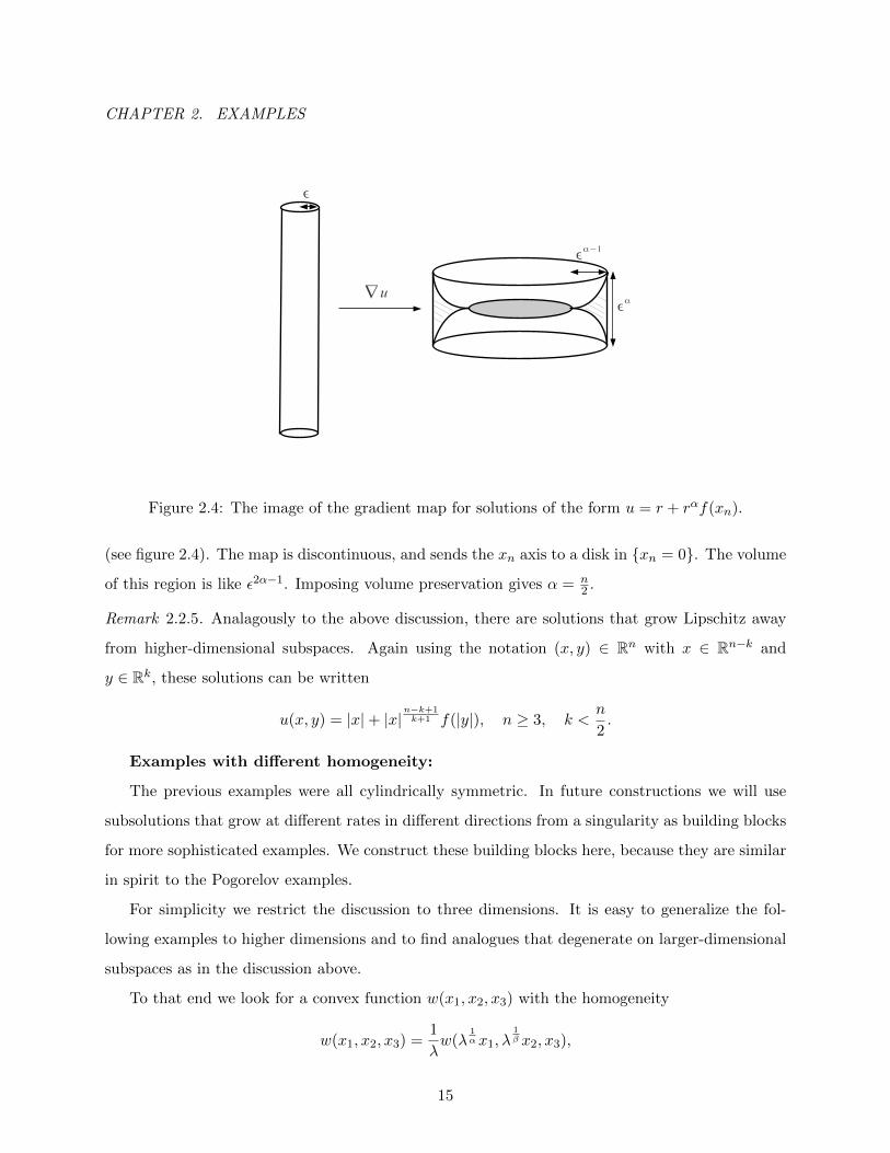
(see figure 2.4). The map is discontinuous, and sends the xn axis to a disk in xn = 0. The volume
of this region is like ε2α−1. Imposing volume preservation gives α = n2 .
Remark 2.2.5. Analagously to the above discussion, there are solutions that grow Lipschitz away
from higher-dimensional subspaces. Again using the notation (x, y) ∈ Rn with x ∈ Rn−k and
y ∈ Rk, these solutions can be written
u(x, y) = |x|+ |x|n−k+1k+1 f(|y|), n ≥ 3, k <
n
2.
Examples with different homogeneity:
The previous examples were all cylindrically symmetric. In future constructions we will use
subsolutions that grow at different rates in different directions from a singularity as building blocks
for more sophisticated examples. We construct these building blocks here, because they are similar
in spirit to the Pogorelov examples.
For simplicity we restrict the discussion to three dimensions. It is easy to generalize the fol-
lowing examples to higher dimensions and to find analogues that degenerate on larger-dimensional
subspaces as in the discussion above.
To that end we look for a convex function w(x1, x2, x3) with the homogeneity
w(x1, x2, x3) =1
λw(λ
1αx1, λ
1β x2, x3),
15
CHAPTER 2. EXAMPLES
where α and β satisfy 1 < α, β < 2 and
1
α+
1
β=
3
2.
We chose this constant so that the homogeneity respects the scaling of the Monge-Ampere equation:
detD2w(x1, x2, x3) = λ2(
1α
+ 1β
)−3
detD2w(λ1αx1, λ
1β x2, x3).
Note that the rescaling (x1, x2)→ (λ1αx1, λ
1β x2) preserves the curves x2 = mx
α/β1 .
Let f(x) denote 1 + x2. An obvious candidate for w is
w(x1, x2, x3) = (xα1 + xβ2 )f(x3).
One checks that
detD2w = |x1|2α−2|x2|β−2(2αβ(α− 1)(β − 1)f2 − 4α2β(β − 1)fx2
3
)+ |x1|α−2|x2|2β−2
(2αβ(α− 1)(β − 1)f2 − 4αβ2(α− 1)fx2
3
).
Then for x3 small depending on α, β we have
detD2w ≥ c(α, β)(|x1|2α−2|x2|β−2 + |x1|α−2|x2|2β−2).
Along the curves x2 = mxα/β1 , we compute
detD2w ≥ c(|m|β−2 + |m|2β−2) ≥ c(α, β),
since 1 < β < 2.
Thus, up to rescaling the x3-axis and multiplying by a constant, we have
detD2w ≥ 1 in Ω = |x′| < 1 × (−1, 1).
In chapter 4 we construct a function g on ∂Ω such that translations and “tiltings” of w touch
g from below at many pairs of points on the top and bottom of Ω. The solution to the Dirichlet
problem detD2u = 1, u|∂Ω = g inherits the singularity of w on the lines connecting such pairs. By
taking α very close to 2, we can produce singular sets of any Hausdorff dimension less than n− 1.
Theorem 1.4.1 shows that this is optimal.
In addition, for any ε > 0, by taking α close enough to 2 we produce solutions that are not in
W 2,1+ε, which shows that W 2,1 regularity is the best we can expect (see chapter 6). See also [M1]
for proofs of these results.
16
CHAPTER 2. EXAMPLES
Remark 2.2.6. One can also construct subsolutions that grow just logarithmically faster than
quadratic away from a singularity in some direction. These subsolutions are
w(x′, x3) = g(x′)
(1 +
x23
| log g(x′)|
),
where
g(x1, x2) = x21| log x1|α +
|x2|| log x2|β
.
In chapter 6 we use these to construct singular solutions to detD2u = 1 with a singular set with
Hausdorff dimension exactly n − 1, and which have second derivatives in L logc L for c small but
not L log20 L, which shows that Theorem 1.4.3 is optimal. See also [M2] for these results.
17
CHAPTER 3. PRELIMINARIES
Chapter 3
Preliminaries
In this chapter we combine the affine invariance of the Monge-Ampere equation with convexity to
obtain some useful localization properties of level sets.
In the first section of this chapter we recall the definition of Alexandrov solutions. In the second
section we prove some results from convex analysis including John’s lemma on the equivalence of
convex sets to ellipsoids, and the Alexandrov maximum principle. We combine these results with
the affine invariance of the Monge-Ampere equation in the third section to control the geometry of
level sets for solutions with certain bounds on the right hand side. Finally, in the last section we
use these observations to prove some previous results on the geometry of singularities.
3.1 Alexandrov solutions
We first recall the notions of Alexandrov solution and sections of convex functions.
Let v be a convex function on Ω ⊂ Rn. We say p ∈ Rn is a subgradient of v at x if it is the
slope of some supporting hyperplane to the graph of v at x. The function v has an associated Borel
measure Mv, called the Monge-Ampere measure, defined by
Mv(A) = |∂v(A)|
where |∂v(A)| represents the Lebesgue measure of the set of subgradients of v in A (see [Gut] for
details). If v ∈ C2, then
|∂v(A)| =∫A
detD2v dx.
18
CHAPTER 3. PRELIMINARIES
Given a Borel measure µ, we say that v is an Alexandrov solution to detD2v = µ if Mv = µ.
It is easy to check that if µ = f dx, then for an invertible linear map L the function v =
| det(L)|−2/nu(Lx) solves
detD2v = f(Lx),
i.e. the Monge-Ampere equation is affine invariant.
We define the sections Svh,p(x) of v by
Svh,p(x) = y ∈ Ω : v(y) < v(x) + p · (y − x) + h
for some subgradient p at x. Geometrically, for this is the set carved out by taking the tangent
plane of slope p at x and lifting it by height h. If Svh,p(x) is compactly contained in Ω then it is
convex, and furthermore if Ω is convex, then any section is convex.
3.2 General results on convex sets and functions
We now discuss some useful results from convex analysis.
John’s lemma says that convex subsets of Rn are equivalent to ellipsoids. This observation
allows us to exploit the affine invariance of the Monge-Ampere equation.
Lemma 3.2.1 (John’s lemma). Let K be a bounded convex subset of Rn with nonempty interior.
Then there exists a point x ∈ K and an ellipsoid E centered at 0 such that
1
nE ⊂ K − x ⊂ E.
Proof. Let E be the ellipsoid of smallest volume containing K and translate so that 0 is the center
of E. We claim that K contains the 1n -times dilation of E.
First, the conclusion of the theorem is invariant under affine transformations so we may assume
that E = B1. Let Bd be the largest ball contained in K. Using the convexity of K and rotating
we may assume that K ⊂ xn ≥ −d. The strategy is to compute the volume of the “squeezed”
ellipsoid Eε with center εen that goes through en and ∂B1∩xn = −d. This ellipsoid has boundary
given algebraically by
∂Eε =
|x′|2
a2+
(xn − ε)2
(1− ε)2= 1
where a is the horizontal axis length.
19
CHAPTER 3. PRELIMINARIES
Inserting |x′|2 = 1− d2 and xn = −d and doing a short computation we obtain
1
a2= 1− 2ε
d
1− d+O(ε2).
We thus have|Eε||B1|
= (1− ε)(
1
a2
)−n−12
= 1− ε(
(n− 1)d
1− d− 1
)+O(ε2).
The coefficient of ε is strictly negative if d < 1n , contradicting the definition of E and proving the
lemma.
We call x + 1nE the John ellipsoid of K. There is some linear transformation A such that
A(B1) = E, and we say that A normalizes K.
Remark 3.2.2. The dilation factor 1n appearing in John’s lemma is optimal. For example, in R2
equality is attained for triangles. More generally, in Rn equality is attained for convex polyhedra
with n+ 1 faces.
Remark 3.2.3. The approximating ellipsoid can also be centered at the center of mass of K, at the
expense of dilating by 1n3/2 . To see this, take the ellipsoid of smallest volume centered at the center
of mass of K and containing K, normalize it to be B1, and rotate so that K ⊂ xn ≥ −d. The
point is that since 0 is the center of mass, K is squeezed from above as well. Indeed, one computes
that K ⊂ |xn| < nd. Using a similar computation to the one above, one shows that the squeezed
ellipsoid centered at 0 with vertical axis length 1 − ε and going through ∂B1 ∩ |xn| = nd has
volume smaller than |B1| if d < 1n3/2 and ε is small, a contradiction.
The Alexandrov maximum principle gives a modulus of continuity for a convex function at the
boundary of a sublevel set in terms of the Monge-Ampere mass and geometry of this set.
Lemma 3.2.4. Let v be a convex function on a bounded domain Ω ⊂ Rn with v|∂Ω = 0. Let D be
the diameter of Ω and for x ∈ Ω, let d(x) denote the distance from x to ∂Ω. Then
|v(x)|n ≤ C(n)d(x)Dn−1Mv(Ω).
Proof. Let C(x) be the function whose graph is the cone generated by (x, v(x)) and ∂Ω. It is easy
to see that ∂C(x) is a convex set containing a ball of radius |v(x)|D centered at 0 and a point a
distance |v(x)|d(x) from 0, giving
|∂C(x)| ≥ c(n)|v(x)|n
Dn−1d(x).
20
CHAPTER 3. PRELIMINARIES
Furthermore, by convexity
∂C(x) ⊂ ∂v(Ω).
The estimate follows.
Finally, we give a variant of the Alexandrov maximum principle which controls the minimum
value of a convex function on a sublevel set in terms of the Monge-Ampere mass and volume of the
set.
Lemma 3.2.5. Let v be a convex function on a bounded domain Ω ⊂ Rn with v|∂Ω = 0. Then
Mv(Ω) |Ω| ≥ c(n)|minΩv|n.
Proof. The estimate is affine invariant, so by John’s lemma we may assume that B1 ⊂ Ω ⊂ Bn. Let
x0 be the point where |v| achieves its maximum and let K(x) be the function whose graph is the
cone generated by (x0, v(x0)) and ∂Bn. Then ∂K(x0) contains a ball of radius at least c(n)|v(x0)|
so we have
|∂K(x0)| ≥ c(n)|v(x0)|n.
Finally, by convexity ∂K(x0) ⊂ ∂v(Ω) and the conclusion follows.
3.3 Localization properties of sections
When we have control on the Monge-Ampere measure of a convex function, we can combine it with
the results above to obtain control on the geometry of level sets.
The first result says that if the right hand side is bounded below by a positive constant then we
have an upper bound on the volume, even if the section is not compactly contained in our domain.
Lemma 3.3.1. Assume that detD2u ≥ λ in a bounded convex domain Ω ⊂ Rn. Then if Suh,p(x) is
any section of u, we have
|Suh,p(x)| ≤ C(n, λ)hn/2.
Proof. Assume by translation that 0 is the center of the John ellipsoid for Suh,p(x). By subtracting
a linear function we can assume that
p = 0, u|∂Suh,0(x) ≤ 0, and | minSuh,0(x)
u| = h.
21
CHAPTER 3. PRELIMINARIES
By John’s Lemma, there is a linear transformation A that normalizes Suh,0(x). Let
u(x) = |detA|−2/nu(Ax).
It is easy to check that
detD2u ≥ λ, u|∂Ω ≤ 0
and B1 ⊂ Ω ⊂ BC(n). Then λ1/n
2 (|x|2 − 1) is an upper barrier for u, so
|minΩu| ≥ c.
Since |detA| ≥ c(n)|Suh,0(x)|, the conclusion follows.
The next result, due to Caffarelli ([C1]), says that if in addition the right hand side is bounded
above, then compactly contained sections Sh(x) are “balanced” around x and we control the volume
from both sides.
Lemma 3.3.2. Assume that λ ≤ detD2u ≤ Λ in Ω ⊂ Rn. Then there exist c, C(n, λ,Λ) such that
for all Suh,p(x) ⊂⊂ Ω, there is an ellipsoid E centered at 0 of volume hn/2 with
cE ⊂ Suh,p(x)− x ⊂ CE.
Proof. Normalize exactly as in the beginning of the proof of lemma 3.3.1, and let x = A−1x. Then
λ1/n
2 (|x|2 − 1) and Λ1/n
2
(|x|2n2 − 1
)are upper and lower barriers, respectively, for u. This gives
c ≤ |u(x)| ≤ C,
hence
chn/2 ≤ |detA| ≤ Chn/2.
Finally, by the Alexandrov maximum principle we have
d(x, ∂Ω) > c.
We conclude that
Bc(x) ⊂ Ω ⊂ BC(x),
and scaling back proves the lemma.
22
CHAPTER 3. PRELIMINARIES
Finally, using similar techniques and the results from the next section one can establish the
following engulfing and covering properties of compactly contained sections (see [CG] and [DFS]).
In the following αSuh,p(x) denotes the α-dilation of Suh,p(x) around x.
Lemma 3.3.3. Assume that λ ≤ detD2u ≤ Λ in Ω. Then there exists δ > 0 universal such that:
1. If Suh,p(x) ⊂⊂ Ω then
Suδh,p(x) ⊂ 1
2Suh,p(x).
2. Suppose that for some compact D ⊂ Ω, we associate to each x ∈ D some Suh,p(x) ⊂⊂ Ω. Then
we can find a finite subcollection Suhi,pi(xi)Mi=1 such that Suδhi,pi(xi) are disjoint and
D ⊂ ∪Mi=1Suhi,pi
(xi).
3.4 Previous results on singularities
In this section we describe two important results of Caffarelli on the geometry of a set where a
solution to λ < detD2u ≤ Λ agrees with a tangent plane.
The first says that a singularity cannot have any interior extremal points. It extends to the
boundary of the domain, possibly with some flat edges in the interior.
Proposition 3.4.1. Assume that λ ≤ detD2u ≤ Λ in a domain Ω ⊂ Rn and let l be a linear
function whose graph supports the graph of u. Then the set u = l has no interior extremal points.
Proof. By subtracting a linear function assume that l = 0. Assume by way of contradiction that
u = 0 has an extremal point in Ω. By translating and scaling we may assume that 0 is an
extremal point and Ω = B1. Rotating, we may assume that
u = 0 ∩ xn ≥ 0 = 0
and that for some d, d′ > 0, the solution u is strictly positive in (B1 − B1−d′) ∩ xn > −d. Let
lε = ε(xn + d). Then the sets Sε = u < lε are compactly contained in B1 for ε sufficiently small.
Write Sε = Suh,p(y) for some h, p, y depending on ε.
We first argue that yn ≥ 0. Indeed, since u ≥ 0, the maximum of lε − u in xn ≤ 0 occurs on
xn = 0. By lemma 3.3.2, Suh,p(y) has points in xn ≥ cd.
23
CHAPTER 3. PRELIMINARIES
However, since u > 0 in xn > 0, we have
Sε ⊂ xn < o(1)
which contradicts the balancing of sections.
Remark 3.4.2. We saw in previous chapters that the key obstruction to regularity is the loss of
strict convexity. The importance of Proposition 3.4.1 is that it implies that solutions with linear
boundary data are strictly convex and C1,α with a quantitative interior estimate. The idea is
that for a general convex function, 12S
uh,p(x) ⊂ Suh/2,p(x), but using a compactness argument and
Proposition 3.4.1 we can improve the dilation constant on the left to 1+δ2 . Rescaling and iterating
gives the result.
Remark 3.4.3. One can in fact show using proposition 3.4.1 and the volume estimate lemma 3.3.1
that if the boundary data are C1,β for β > 1− 2n then solutions are strictly convex. Indeed, since a
singularity doesn’t have extremal points it contains a line segment that hits the boundary at both
ends. If the boundary data were C1,β then the volume of the section of height h taken with the
plane that agrees with u on this segment is of order hn−11+β , since the section has length of order 1
for all h. The volume estimate gives the conclusion.
Finally, the last result of this chapter says that if the right side is bounded below by a positive
constant, then the set where u agrees with a tangent plane has affine dimension strictly less than
n2 . In light of the examples from chapter 2, this estimate is sharp. Caffarelli proved this result in
[C3]. We provide a short proof using a technique related to our proof of theorem 1.4.1. The idea is
that if the agreement set has large dimension, then even if u grows as fast as possible (Lipschitz) in
the remaining directions, we can find a section whose volume is too large by “tilting” the tangent
plane. This proof can also be found in [M1].
Lemma 3.4.4. Assume
detD2u ≥ λ > 0
in B1 ⊂ Rn. Then u cannot vanish on a subspace of dimension n2 or higher.
Proof. Suppose u vanishes on
xk+1 = ... = xn = 0 ∩B1.
24
CHAPTER 3. PRELIMINARIES
By subtracting a linear function of the form ak+1xk+1+...+anxn we may assume that u(ten) = o(t).
Then Suh,0(0) has length R(h)h in the en direction, where R(h)→∞ as h→ 0. Furthermore, Suh,0(0)
has length exceeding 1Ch in the en−k, ..., en−1 directions, where C is the Lipschitz constant of u in
B1/2. Finally, Suh,0(0) contains the unit ball in the subspace spanned by e1, ..., ek. We conclude
that
|Suh,0(0)| ≥ C−kR(h)hn−k,
which contradicts Lemma 3.3.1 as h→ 0 for k ≥ n2 .
Remark 3.4.5. Lemma 3.4.4 implies in particular that every solution to detD2u ≥ 1 in two dimen-
sions is strictly convex.
25
CHAPTER 4. PARTIAL REGULARITY
Chapter 4
Partial Regularity
Recall that we say that a convex function u is strictly convex at x if some supporting plane touches
u only at x. In this chapter we prove theorem 1.4.1, which says that if detD2u is bounded below
by a positive constant, then u is strictly convex away from a small singular set of Hausdorff n− 1
dimensional measure zero.
Previous results on the singularities of convex functions include those of Alberti, Ambrosio and
Cannarsa (see [A], [AAC]), who show that the nondifferentiability set of a semi-convex function
is n − 1 rectifiable. Theorem 1.4.1 may be viewed as a strengthening of this result when we have
positive lower and upper bounds on detD2u, in which case Caffarelli’s regularity theory gives
differentiability at points of strict convexity (see chapter 3). In fact, if detD2u = 1 then Σ is
precisely the set where u is not smooth. However, it is important to note that points in Σ may
still be points of differentiability for u (see for example the Pogorelov solutions in chapter 2), and
without an upper bound on detD2u the points of non-differentiability for u may not be in Σ (take
for example u = |x|2 + |xn|, which solves detD2u ≥ 1 and is strictly convex everywhere).
The chapter is organized as follows. In the first section we prove theorem 1.4.1 using the results
on section geometry from chapter 3 and the useful technique of replacing u by u+ 12 |x|
2. The key
estimate shows that u grows much faster than quadratically in at least two directions perpendicular
to a singular line. In the last section we construct, for any δ small, a solution to detD2u = 1 with
a singular set of Hausdorff dimension n− 1− δ, which shows that our partial regularity theorem is
optimal.
26
CHAPTER 4. PARTIAL REGULARITY
4.1 Proof of Theorem 1.4.1
In this section assume that
detD2u ≥ 1
in B1 ⊂ Rn. Fix x ∈ Σ and a subgradient p at x. By translation and subtracting a linear function
assume that x = p = 0. Then u = 0 contains a line segment of some length l. By Lemma 3.3.1,
|Suh,0(0)| ≤ C(n)hn/2
for all h > 0.
Letting v = u+ 12 |x|
2, it follows that
|Svh,0(0)| ≤ C(n)
lhn+1
2
for all h small. In fact, for any x0 ∈ Σ and subgradient p0 to v at x0 we have
|Svh,p0(x0)| < Ch
n+12
for some C which may depend on x0 and p0. Indeed, p0 can be written as p+x0 for some subgradient
p of u at x0, and one easily checks that
Svh,p0(x0) = S
u+ 12|x−x0|2
h,p (x0),
so by subtracting a linear function with slope p and translating we are in the situation described
above.
Theorem 1.4.1 thus follows from the following more general result:
Theorem 4.1.1. Let v be any convex function on B1 ⊂ Rn with sections Svh,p, and let Σv denote
the set of points x such that for all subgradients p at x, there is some Cx,p such that
|Svh,p(x)| < Cx,phn+1
2
for all h small. Then
Hn−1(Σv) = 0.
27
CHAPTER 4. PARTIAL REGULARITY
Proof of Theorem 1.4.1: Let v = u + 12 |x|
2. By the discussion preceding the statement of
Theorem 4.1.1, Σ ⊂ Σv. The conclusion follows from Theorem 4.1.1.
We briefly discuss the main ideas of the proof. Fix x ∈ Σv and a subgradient p at x. In
the following analysis c, C will denote small and large constants depending on n and Cx,p. If
Svh,p(x) ⊂⊂ B1 then the definition of Σv and Lemma 3.2.5 give
Mv(Svh(x)) ≥ chn−1
2 = c(h1/2)n−1 (4.1)
for all h small.
An important technique of the proof is to replace v by v + 12 |x|
2. Since adding a quadratic can
only decrease section volume, we have
Σv ⊂ Σv+ 12|x|2
and it suffices to prove Theorem 4.1.1 for this case. Then all of the sections are compactly contained
in B1 for h small, and the diameter of sections is at most h1/2. By replacing the sections Svh,p(x)
by B√h(x) and using a covering argument, we easily obtain that Σv has Hausdorff dimension at
most n− 1.
Lemmas 4.1.2 and 4.1.3 improve this result as follows. We aim to rule out behavior like
|x|2 + |xn|,
which has a singular hyperplane. For this example, the sections at xn = 0 have the correct
growth when we take supporting slopes with no xn-component, but the sections are too large when
we take supporting slopes with xn-component 1.
In the first lemma we use that the sections are small for all supporting planes at x ∈ Σv to
show that v must grow much faster than quadratically in at least two directions, unlike the example
above:
Lemma 4.1.2. Assume that v = v0 + 12 |x|
2 for some convex function v0. Fix x ∈ Σv. For a
supporting slope p of v at x, let
d1(h) ≥ d2(h) ≥ ... ≥ dn(h)
28
CHAPTER 4. PARTIAL REGULARITY
denote the axis lengths of the John ellipsoid of the section Svh,p(x). Then
dn−1(h)
h1/2→ 0 as h→ 0.
The heuristic idea is that if not, then u resembles |x|2 + xn in some system of coordinates, and
by tilting the tangent plane we get sections whose volumes are too large.
In the second lemma we use the above observation about the Monge-Ampere mass of v (inequal-
ity 4.1) in the directions where v grows much faster than quadratically from x. Since we replaced
v by v + 12 |x|
2 we also know that v grows at least quadratically in the remaining directions. This
allows us to cover Σv with balls in which the Monge-Ampere mass of v is much larger than the
radius to the n− 1, giving the desired improvement.
Lemma 4.1.3. Assume that v = v0 + 12 |x|
2 for some convex function v0. Fix x ∈ Σv. For any
ε > 0, there is a sequence rk → 0 such that
Mv(Brk(x)) >1
εrn−1k .
The proof of Theorem 4.1.1 follows easily from Lemma 4.1.3.
Proof of Theorem 4.1.1: Since Σv ⊂ Σv+ 12|x|2 , we may assume without loss of generality that v
has the form v0 + 12 |x|
2 with v0 convex.
Fix ε small. By Lemma 4.1.3, for each x ∈ Σv we can choose an arbitrarily small r such that
Mv(Br(x)) >1
εrn−1.
Cover Σv ∩ B1/2 with such balls, and choose a Vitali subcover Bri(xi)Ni=1, i.e. a disjoint subcol-
lection such that B3ri(xi) cover Σv ∩B1/2. Then
N∑i=1
(3ri)n−1 ≤ Cε
N∑i=1
Mv(Bri(xi))
≤ Cε,
since v is locally Lipschitz and the Bri are disjoint. This means exactly that
Hn−1(Σv ∩B1/2) = 0.
29
CHAPTER 4. PARTIAL REGULARITY
The above reasoning also gives Hn−1(Σv ∩B1−β) = 0 for any β small, but not necessarily for β = 0
since we only know v is locally Lipschitz. To get
Hn−1(Σv ∩B1) = 0,
use that Σv ∩B1 = ∪∞k=1Σv ∩B1−1/k and apply countable subadditivity.
We now prove Lemmas 4.1.2 and 4.1.3.
Proof of Lemma 4.1.2: By translating and subtracting a linear function assume that x = p = 0.
Assume by way of contradiction that we can find hk → 0 and some δ > 0 such that
dn−1(hk) > δh1/2k (4.2)
for all k. We first show that v is trapped by two tangent planes at 0.
Let x1,k and x2,k be the points on ∂Svhk,0(0) where the hyperplanes perpendicular to the shortest
axis of the John ellipsoid become tangent to ∂Svhk,0(0), and let p1,k and p2,k denote subgradients at
these points. Since
d1(hk)d2(hk)...dn(hk) < Chn+1
2k ,
we have by the inequality 4.2 that dn(hk) <C
δn−1hk for all k. By this observation and convexity we
can rotate and pass to a subsequence such that
p1,k → c1(δ)en, p2,k → −c2(δ)en.
Then v is trapped by the planes ±c(δ)xn. We conclude that
Svhk,0(0) ⊂ |xn| < C(δ)hk.
To complete the proof, we show that the volumes of sections obtained with tilted supporting
planes are too large. Take the largest a such that v ≥ axn and consider the sections
Sk = Sv(1+aC(δ))hk,aen(0).
Then Sk engulf Svhk,0(0). Furthermore,
sup|xn| : x ∈ Sk = Rkhk,
30
CHAPTER 4. PARTIAL REGULARITY
where Rk → ∞ as k → ∞. Indeed, if not, then for some small ε and a sequence bi → 0 we would
have v(x′, bi) > (a+ ε)bi for all x′. Convexity and v(0) = 0 imply that v > (a+ ε)xn for all xn > bi,
which in turn implies that
v > (a+ ε)xn,
contradicting the definition of a.
Finally, let xk = (x′k, Rkhk) ∈ Sk be the point in Sk furthest in the en direction. Since v grows
at least quadratically away from every tangent plane, we have
|x′k| < C(δ, a)h1/2k . (4.3)
Explicitly, since aen is a subgradient at 0 and v is of the form v0 + 12 |x|
2 with v0 convex, we have
that aen is a subgradient of v0 at 0, giving
axn +1
2|x|2 ≤ v ≤ C(δ, a)hk + axn
in Sk, giving the desired bound on |x′k|.
Recall that
Svhk,0(0) ⊂ |xn| < C(δ)hk ∩Bh1/2k
(0).
Take any two points y, z in |xn| < C(δ)hk ∩Bh1/2k
(0) a distance δh1/2k apart, take the lines from
these points to (x′k, Rkhk) and denote the intersections of these lines with xn = C(δ)hk by y and
z. Since |yn − zn| < Chk and |y − z| > δh1/2k , it is obvious that |y′ − z′| > δ
2h1/2k for k large. By
similar triangles and inequality 4.3, we also have
|y′ − y′| = C
Rk|y′ − x′k| ≤
C
Rkh
1/2k ,
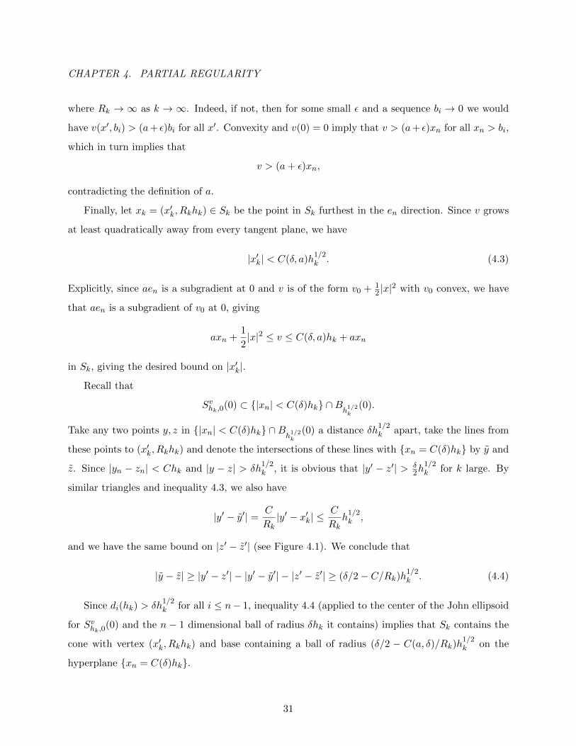
and we have the same bound on |z′ − z′| (see Figure 4.1). We conclude that
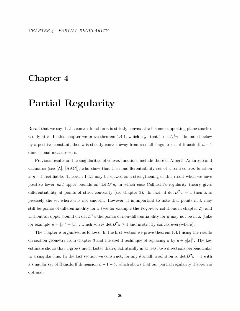
|y − z| ≥ |y′ − z′| − |y′ − y′| − |z′ − z′| ≥ (δ/2− C/Rk)h1/2k . (4.4)
Since di(hk) > δh1/2k for all i ≤ n− 1, inequality 4.4 (applied to the center of the John ellipsoid
for Svhk,0(0) and the n− 1 dimensional ball of radius δhk it contains) implies that Sk contains the
cone with vertex (x′k, Rkhk) and base containing a ball of radius (δ/2 − C(a, δ)/Rk)h1/2k on the
hyperplane xn = C(δ)hk.
31
CHAPTER 4. PARTIAL REGULARITY
<Ch k1 /2
<Ch k1 /2 /Rk
>δhk1 /2
>(δ /2)hk1 /2
Rk hk
C hk
S hk ,0v
(0)
yzzzy
x k
Figure 4.1: The cone above xn = Chk generated by xk and the John ellipsoid of Svhk,0(0) has a
base containing a ball of radius at least (δ/2− C(a, δ)/Rk)h1/2k .
We conclude that
|Sk| ≥ c(δ, a)Rkhn+1
2k ,
contradicting our definition of Σv for k large.
Proof of Lemma 4.1.3: Fix a subgradient p at x and let d1(h), ..., dn(h) be defined as in the
statement of Lemma 4.1.2. Let
I = min
i :di(h)
h1/2→ 0 as h→ 0
.
Fix δ small. Then we can find a sequence hk → 0 and η depending only on p such that
dI(hk) < δh1/2k , (4.5)
and
di(hk) > ηh1/2k (4.6)
for all i < I. Rotate the axes so that the ei are the axes for the John ellipsoid of Svhk,p(x) and
assume by translation that x = 0.
32
CHAPTER 4. PARTIAL REGULARITY
Take the restriction of v to the subspace spanned by eI , ..., en, and call this restriction w. Let
Swk = Svhk,p(x) ∩ x1 = ... = xI−1 = 0,
the slice of the section Svhk,p(x) in this subspace. Then since
d1(hk)d2(hk)...dn(hk) ≤ Chn+1
2k
and v grows at most quadratically in the first I − 1 directions (inequality 4.6), we have
|Swk |Hn−I+1 ≤C
ηI−1hn+2−I
2k .
Using this and Lemma 3.2.5,
Mw(Swk ) ≥ cηI−1hn−I
2k . (4.7)
Finally, let rk = C(n)dI(hk), with C(n) taken large enough that
Swk ⊂ Brk/2(x).
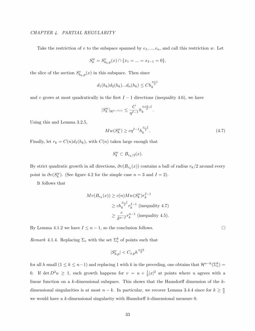
By strict quadratic growth in all directions, ∂v(Brk(x)) contains a ball of radius rk/2 around every
point in ∂v(Swk ). (See figure 4.2 for the simple case n = 3 and I = 2).
It follows that
Mv(Brk(x)) ≥ c(n)Mw(Swk )rI−1k
≥ chn−I
2k rI−1
k (inequality 4.7)
≥ c
δn−Irn−1k (inequality 4.5).
By Lemma 4.1.2 we have I ≤ n− 1, so the conclusion follows.
Remark 4.1.4. Replacing Σv with the set Σkv of points such that
|Svh,p| < Cx,phn+k
2
for all h small (1 ≤ k ≤ n−1) and replacing 1 with k in the preceding, one obtains that Hn−k(Σkv) =
0. If detD2u ≥ 1, such growth happens for v = u + 12 |x|
2 at points where u agrees with a
linear function on a k-dimensional subspace. This shows that the Hausdorff dimension of the k-
dimensional singularities is at most n − k. In particular, we recover Lemma 3.4.4 since for k ≥ n2
we would have a k-dimensional singularity with Hausdorff k-dimensional measure 0.
33
CHAPTER 4. PARTIAL REGULARITY
B r k /2( y)
S kw ∇(v )
∇(v )(S kw)
∇(v )(B r k/2( y))
B r k( x) , r k2 << h
Figure 4.2: ∇v(Brk(x)) contains an rk/2-neighborhood of the surface ∇v(Swk ), which projects in
the e1 direction (down) to a set of H2 measure at least cδ rk.
4.2 Example showing optimality of Theorem 1.4.1
In this section we construct examples of solutions to detD2u = 1 in R3 such that Σ has Hausdorff
dimension as close to 2 as we like. A small modification produces the analagous examples in Rn.
For this section, fix δ > 0 small. We construct our examples in several steps, which we briefly
describe:
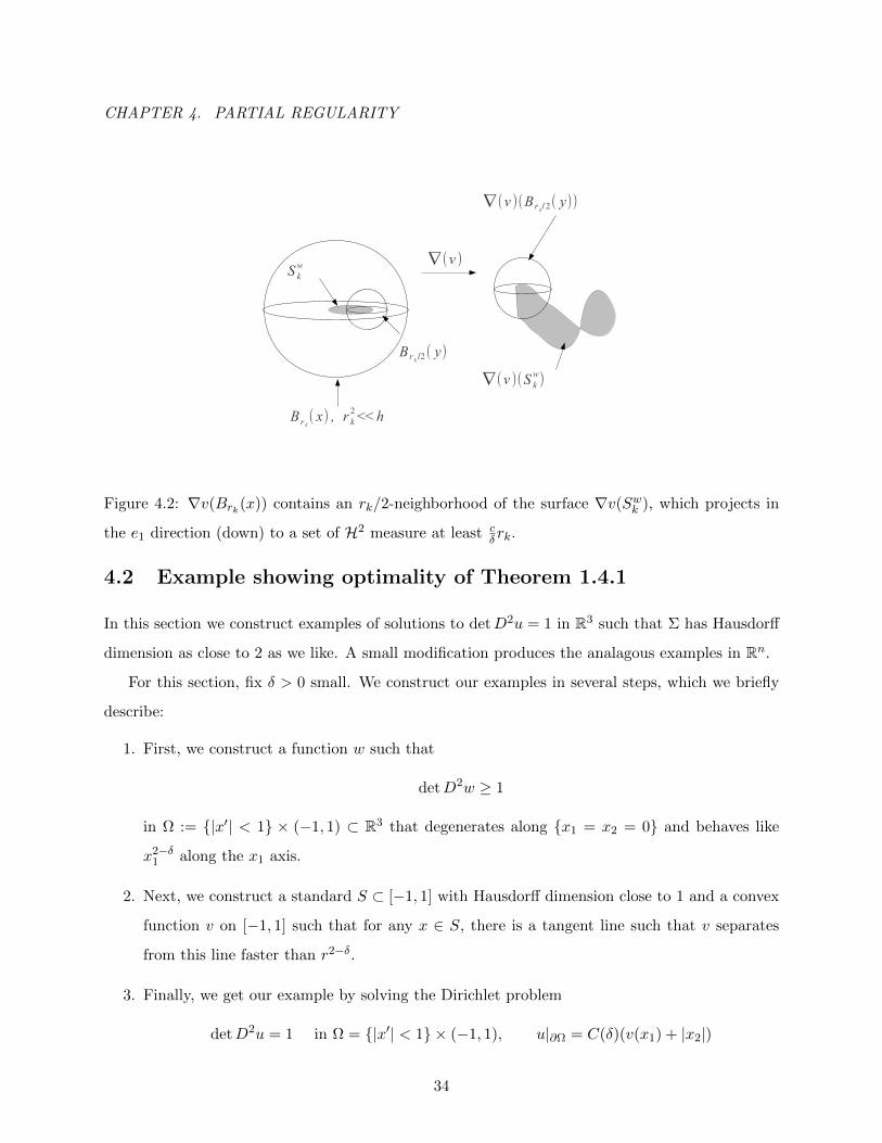
1. First, we construct a function w such that
detD2w ≥ 1
in Ω := |x′| < 1 × (−1, 1) ⊂ R3 that degenerates along x1 = x2 = 0 and behaves like
x2−δ1 along the x1 axis.
2. Next, we construct a standard S ⊂ [−1, 1] with Hausdorff dimension close to 1 and a convex
function v on [−1, 1] such that for any x ∈ S, there is a tangent line such that v separates
from this line faster than r2−δ.
3. Finally, we get our example by solving the Dirichlet problem
detD2u = 1 in Ω = |x′| < 1 × (−1, 1), u|∂Ω = C(δ)(v(x1) + |x2|)
34
CHAPTER 4. PARTIAL REGULARITY
and comparing with w at points in S × 0 × ±1.
In the following analysis c and C will denote small and large constants depending on δ.
Construction of w: Let w be the subsolution constructed at the end of chapter 2 with
α = 2− δ. (Recall that w is a rescaling of the function C(xα1 + xβ2 )(1 + x23) with 1
α + 1β = 3
2). Then
detD2w ≥ 1 in Ω and has the desired growth in the x1 direction.
Construction of S: Let ε > 0 be a small constant we will choose shortly depending on
δ. Construct a self-similar set in [−1/2, 1/2] as follows: First, remove an open interval of length
γ = 1 − 2−3ε from the center. Proceed inductively by removing intervals a fraction γ of each of
those that remains. Denote the centers of the intervals removed at stage k by xi,k2k−1
i=1 , and the
intervals by Ii,k. Finally, let
S = [−1/2, 1/2]− ∪i,kIi,k.
It is easy to check that |Ii,k+1| = γ2−(1+3ε)k and that S has Hausdorff dimension 11+3ε .
Construction of v: Let
v0(x) =
|x| |x| ≤ 1
2|x| − 1 |x| > 1
We add rescalings of v0 together to produce the desired function:
v(x) =
∞∑k=1
2k−1∑i=1
2−2(1+2ε)kv0(2γ−12(1+3ε)k(x− xi,k)).
We now check that v satisfies the desired properties:
1. v is convex, as the sum of convex functions. Furthermore,
|v(x)| ≤ C∞∑k=1
2k−1∑i=1
2−(1+ε)k
≤ C∞∑k=1
2−εk,
so v is bounded.
2. Let x ∈ S. We aim to show that v separates from a tangent line more than r2−δ a distance r
from x. By subtracting a line assume that v(x) = 0 and that 0 is a subgradient at x. Assume
further that x + r < 1/2 and that 2−(1+3ε)k < r ≤ 2−(1+3ε)(k−1). There are two cases to
examine:
35
CHAPTER 4. PARTIAL REGULARITY
Case 1: There is some y ∈ (x+ r/2, x+ r) ∩ S. Then by the construction of S it is easy to
see that there is some interval Ii,k+2 such that Ii,k+2 ⊂ (x, x + r). On this interval, v grows
by
2−2(1+2ε)(k+2) ≥ cr2 1+2ε1+3ε = cr2−δ,
where we choose ε so that
δ =2ε
1 + 3ε.
Case 2: Otherwise, there is an interval Ii,j of length exceeding r/2 such that (x+r/2, x+r) ⊂
Ii,j . In particular, j ≤ k + 2. Then at the left point of Ii,j , the slope of v jumps by at least
2−(1+ε)(k+2). It follows that at x+ r, v is at least
r
22−(1+ε)(k+2) ≥ cr2−δ.
Thus, v has the desired properties.
Construction of u: We recall the following lemma on the solvability of the Monge-Ampere
equation (see [Gut],[Har]).
Lemma 4.2.1. If Ω is open, bounded and convex, µ is a finite Borel measure on Ω and g is
continuous and convex in Ω then there exists a unique convex solution u ∈ C(Ω) to the Dirichlet
problem
detD2u = µ, u|∂Ω = g.
Let g(x1, x2, x3) = C(v(x1) + |x2|) for a constant C depending on δ we will choose shortly, and
obtain u by solving the Dirichlet problem
detD2u = 1 in Ω = |x′| < 1 × [−1, 1], u|∂Ω = g.
Take z = (z1, 0, 0) for z1 ∈ S, and let az be a subgradient of v at z1. Let
wz(x) = g(z) + az(x1 − z1) + w(x− z).
Since
w(x− z) ≤ C0(|x1 − z1|2−δ + |x2|β)
36
CHAPTER 4. PARTIAL REGULARITY
for some C0, we can take C large so that
g(x1, x2,±1) ≥ g(z) + az(x1 − z1) + C(|x1 − z1|2−δ + |x2|) ≥ wz(x1, x2,±1)
on the top and bottom of Ω. Furthermore, since g is independent of x3 and for any fixed x′ we
know wz takes its maxima at (x′,±1), we have g ≥ wz on all of ∂Ω. Thus, u ≥ wz in all of Ω. Since
u takes the value g(z) at (z1, 0,±1) and wz(z1, 0, x3) = g(z) for all |x3| < 1, we have by convexity
that u = g(z) along (z1, 0, x3).
We conclude that Σ contains S×0×(−1, 1), which has Hausdorff dimension 1+ 11+3ε = 2− 3
2δ.
Remark 4.2.2. To get the analagous example in Rn, take
u(x1, x2, x3) + x24 + ...+ x2
n.
Observe that this solution has exactly the behavior described by Lemma 4.1.2, which says that u
must grow faster than quadratically in two directions. In chapter 6 we show that for any ε, we can
take δ small enough that these examples are not in W 2,1+ε.
37
CHAPTER 5. UNIQUE CONTINUATION
Chapter 5
Unique Continuation
In this chapter we show that if two (Alexandrov) solutions to detD2u = 1 on B1 agree on a set with
nonempty interior, then they agree everywhere. The difference between the solutions solves a linear
equation with coefficients depending on their second derivatives. If the solutions are smooth then
the coefficients are smooth, and the result follows from a classical unique continuation theorem for
linear equations. However, solutions to the Monge-Ampere equation are not smooth everywhere.
The idea is that by theorem 1.4.1, solutions are smooth on an open dense connected set, so the
classical unique continuation theorem still suffices.
In the first section we discuss the unique continuation theorem for linear equations and prove
one version via Carleman estimates. The key hypothesis is that the coefficients are Lipschitz.
In the next section we use it to prove theorem 1.4.2. Finally, in the last section we construct a
counterexample to linear unique continuation when the coefficients are not Lipschitz.
The first and third sections of this chapter are expository. They included to keep this paper as
self-contained as possible.
5.1 Unique continuation for linear equations
In the first section we discuss a classical unique continuation theorem for linear equations (see e.g.
[H]).
Theorem 5.1.1. Assume that Ω is a connected open domain in Rn and that u solves
aij(x)uij = 0
38
CHAPTER 5. UNIQUE CONTINUATION
in Ω, where 0 < λI ≤ (aij) ≤ 1λI. Assume further that aij are Lipschitz. Then if u = 0 has
nonempty interior, then u vanishes identically.
Remark 5.1.2. In R2, the theorem holds true without any regularity hypotheses on aij . However,
there are counterexamples in higher dimensions (see the last section of this chapter). Unique
continuation also holds when there are lower-order terms with for example bounded coefficients.
Remark 5.1.3. The result is also true if sup∂Br |u| = O(rk) for all k. This property is known as
strong unique continuation. It is not hard to modify the discussion below to obtain this result.
Remark 5.1.4. For linear equations with Lipschitz coefficients, any two solutions which agree on a
set with nonempty interior must agree everywhere. For fully nonlinear uniformly elliptic equations
of the form
F (D2u) = 0
with F in C1,1, the same result is known provided we know one of the two solutions is smooth
([AS]). The idea is to reduce problem to the linear case by showing that the solution is very
close to a paraboloid near some point in the boundary of the agreement set. One can then use
a small-perturbations regularity result of Savin ([S]) to conclude that the solution is smooth in a
neighborhood of this point, and apply theorem 5.1.1 to the linearized equation.
We will discuss a version of unique continuation in which the solution vanishes in a half space to
emphasize ideas and simplify computations. These ideas are not hard to adapt to a radial geometry
to prove strong unique continuation (see remark 5.1.8).
To motivate the idea, consider a harmonic function u on R2 vanishing on the boundary of the
strip 0 ≤ x1 ≤ π. We can “decompose u into frequencies,” writing
u(x′, xn) =∑k
ak sin(kx1)ekx2 .
If |u| is very small for x2 < 0 then the dominant terms oscillate rapidly in x1 and grow rapidly in x2
(i.e. k is large), and if u vanishes near x2 = 0 then there are no nonzero terms in the expansion.
We aim to adapt these ideas to a proof that does not use analyticity.
Assume now that u is harmonic on Rn. The heuristic idea of the Carleman estimates is to
show that the dominant frequency in u is “increasing with xn”. If u vanishes in xn ≤ 0 then its
frequency is “infinite” near xn = 0, so this estimate would imply that u also vanishes for xn > 0.
39
CHAPTER 5. UNIQUE CONTINUATION
To that end, we multiply u by the weights e−λxn , giving a function v whose amplitude (roughly)
represents how much u oscillates with frequency λ, and compute the equation for v. A short
computation gives
0 = e−λxn∆u = ∆v + λ2v + 2λvn.
Let Q denote the cylinder |x′| < 1 × (−1, 1) and assume that u vanishes in Q ∩ xn ≤ 0.
Assume further that u is supported away from ∂Q∩xn ≤ a for some a > 0. We will show that u
vanishes for xn ≤ a, i.e. we can push the zero set a little further up. The strategy is to square the
equation for v and integrate by parts. Pairing vn with the other terms gives only boundary terms
involving some quadratic (vector-valued) polynomial P in λ3/2v and λ1/2∇v. We thus have
λ4
∫Qv2 dx+
∫Q
(∆v)2 dx+ 2λ2
∫Qv∆v dx+ 4λ2
∫Qv2n dx =
∫∂QP (λ3/2v, λ1/2∇v) · ν ds.
Observe that if n = 1 then the last two terms are positive plus a boundary term of the same form.
This gives the inequality
λ4
∫ 1
−1e−2λxu2 dx ≤ Cλ3e−2λ
where C depends on u and its derivative, but not λ. Taking λ to ∞ implies unique continuation
because e−2λx is much larger than e−2λ for x < 1.
In higher dimensions, if we somehow squeezed another µλ4∫Q v
2 dx in this computation, we
could swallow the third term by the first two using that
2λ2|v∆v| ≤ (1− µ/2)(∆v)2 +λ4
1− µ/2v2.
This would give the inequality
λ4
∫Qe−2λxnu2 dx ≤ Cλ3e−2λa
where C depends on u, its derivatives, and µ. Again, taking λ to ∞ would give continuation of the
zero set to xn ≤ a because
e−2λxn >> e−2λa
where xn < a.
We can in fact obtain such an estimate by making the weight slightly concave: we replace e−λxn
by e−λφ(xn) where
φ(xn) = xn −x2n
2.
40
CHAPTER 5. UNIQUE CONTINUATION
This is the main subtlety in the Carleman estimate: to modify the weight so that we get a favorable
term in our integration by parts.
We now state and prove the precise inequality motivated above, for harmonic functions. It
is straightforward to adapt the argument to Lipschitz coefficients and to a radial geometry. We
indicate how in remarks 5.1.7 and 5.1.8.
Proposition 5.1.5. Assume that ∆u = 0 in Q := |x′| < 1 × (−1, 1) and let φ be defined as
above. Then for all λ large we have
λ3
∫Qe−2λφu2 dx ≤
∫∂Qe−2λφP (λ3/2u, λ1/2∇u) · ν ds
where P is some quadratic polynomial.
Note that the homogeneity in λ on the left side is one less than what appears in the discussion
above. If u vanishes in Q ∩ xn ≤ 0 and is supported away from ∂Q ∩ xn ≤ a, then taking λ to
∞, we get continuation of the zero set to xn ≤ a.
The strategy to prove proposition 5.1.5 is the same as that outlined above. We compute the
equation for v = e−λφu, square and integrate by parts. A short computation gives
e−λφ∆u = ∆v + λ2φ′2v2 + λ(2φ′vn − v).
Proposition 5.1.5 follows easily from the following key computation.
Lemma 5.1.6. The following identity holds for any smooth function v, with φ defined as above:∫Q
(∆v + λ2φ′2v + λ(2φ′vn − v))2 dx =
∫Q
(∆v + λ2φ′2v − λ(2φ′vn − v))2 dx
+ 8λ
∫Q
(λ2φ′2v2 + v2n) dx
+ 4λ
∫∂Q
[(2φ′vn − v)∇v + (λ2φ′3v2 − φ′|∇v|2)en)] · ν ds.
Proof. We compute ∫Q
(∆v + λ2φ′2v)(2φ′vn − v).
Pairing the first term in each expression and moving a derivative from ∆v gives
2
∫Qφ′vn∆v dx = 2
∫∂Qφ′vn∇v · ν dx−
∫Qφ′∂n|∇v|2 dx+ 2
∫Qv2n dx
=
∫∂Q
(2φ′vn∇v − φ′|∇v|2en) · ν ds+ 2
∫Qv2n dx−
∫Q|∇v|2 dx.
41
CHAPTER 5. UNIQUE CONTINUATION
Pairing the first term from the first expression and the last from the second gives
−∫Qv∆v dx = −
∫∂Qv∇v · ν +
∫Q|∇v|2 dx.
Pairing the second term from the first expression with the first term from the second expression
gives
λ2
∫Qφ′3∂n(v2) dx = λ2
∫∂Qφ′3v2en · ν ds+ 3λ2
∫Qφ′2v2 dx.
Finally, the last term is
−λ2
∫Qφ′2v2 dx.
Summing them all gives the identity.
Proof of proposition 5.1.5. Let v(x) = e−λφ(xn)u(x). Then the left hand side of identity 5.1.6
is zero, and the boundary term has the desired form.
Remark 5.1.7. The above argument is easy to adapt to the case that aij are Lipschitz. By scaling
we may assume that |aij − δij | < ε and that |∇aij | < ε for some small ε. Computing the equation
for v = e−λφ(xn)u, squaring and integrating by parts, we get the same thing as before plus a small
error of the form
O(ε)
∫Q
(λ3v2 + λ|∇v|2) dx.
The reason we don’t have second derivative errors appearing is because terms of the form AD2v ·Dv
can be rewritten as AD(Dv ·Dv) via integration by parts, up to an error of O(ε)|∇v|2. By using
the favorable terms in the key computation a little more carefully we can cancel this error to get
proposition 5.1.5 for Lipschitz coefficients.
Remark 5.1.8. The previous discussion can be adapted to a radial geometry, and in fact to give
strong unique continuation. The idea is that if u is harmonic then it can be decomposed into
homogeneous harmonic polynomials rkYk(ω) (with r = |x| and ω ∈ ∂B1) whose radial growth rate
corresponds to their “frequency on the sphere.” To measure how much u oscillates spherically with
frequency λ, examine the function
v = ϕ(r)−λu
where ϕ(r) is a perturbation of r chosen to give the correct terms when integrating the equation
for v by parts. One computes
0 =ϕ
ϕ′φ−λ∆u =
ϕ
ϕ′∆v + λ2ϕ
′
ϕv + 2α
ϕ′
ϕw
42
CHAPTER 5. UNIQUE CONTINUATION
where
w =ϕ
ϕ′vr +
1
2
(ϕ′′
ϕ+
(n− 1)ϕ
rϕ′− 1
)v.
Taking ϕ such that ϕrϕ′ = er, and provided sup∂Br |u| = O(rk) for some k > λ, we can square the
equation and integrate by parts to get an analogue to our key computation. This gives a Carleman
estimate of the form ∫B1
ϕ−2λu2 dx ≤ C∫∂B1
ϕ−2λP (λ, u,∇u) ds
where P is some polynomial. If u vanishes to infinite order at 0 we can take λ to ∞, and conclude
that u vanishes identically.
5.2 Proof of Theorem 1.4.2
Assume that u, v satisfy the hypotheses of Theorem 1.4.2. For our proof of unique continuation
we apply theorem 5.1.1 to the difference of u and v, which solves a linear equation where u and
v are sufficiently regular. Indeed, suppose u and v are C2 in a neighborhood of x and let wt be
the convex combination tu + (1 − t)v. Let (Wt)ij be the matrix of cofactors for D2wt. Then by
expanding 0 =∫ 1
0ddt detD2wtdt we get
aij(x)(u− v)ij = 0,
where
aij(x) =
∫ 1
0(Wt)
ij(x)dt.
If the right side is sufficiently regular, then the coefficients are Lipschitz. In particular, f ∈ C1,α
suffices by Caffarelli’s perturbation theory for strictly convex solutions:
Theorem 5.2.1. Assume
detD2u = f in Ω, u|∂Ω = 0
where f ∈ C1,α(Ω) is strictly positive. Then
u ∈ C3,α(Ω).
Finally, we observe that open sets whose complements have zero Hausdorff n − 1 dimensional
measure are connected.
43
CHAPTER 5. UNIQUE CONTINUATION
Lemma 5.2.2. Assume K ⊂ Rn is closed, and assume further that Hn−1(K) = 0. Then Rn −K
is pathwise connected.
Proof. Assume by way of contradiction that D = Rn −K is not pathwise connected. Since D is
open, by rotation, translation and scaling we can assume that the points ±Ren ∈ D cannot be
connected by any continuous path through D and that
|x′| < 1 × ±R ⊂ D.
Let K ′ be the projection of K onto xn = 0 and let B′1 = B1 ∩ xn = 0. If B′1 −K ′ 6= ∅, this
would violate the contradiction hypothesis because then we could find a point x′ ∈ B′1 such that
(x′, t) ∈ D for all t ∈ R and take our path to be the straight lines from −Ren to (x′,−R) to (x′, R)
to Ren.
We conclude that for any cover of K by balls Bri(xi)∞i=1, we have
∑i
rn−1i ≥ 1,
contradicting that Hn−1(K) = 0.
The proof of unique continuation follows easily from these observations and our partial regularity
result theorem 1.4.1.
Proof of Theorem 1.4.2: Let Σu and Σv be the singular sets of u and v respectively, and let
A = Ω− (Σu ∪ Σv). Since A is dense in Ω, it suffices to show that u = v on A.
By Caffarelli’s theory ([C1]), A is an open set. Indeed, for x ∈ A we can find some p in Rn
and h small such that Suh,p(x) ⊂⊂ Ω, and since f is bounded in this section Caffarelli gives that
u is strictly convex in a neighborhood of x. (The same reasoning gives that v is strictly convex in
a neighborhood of x.) By Theorem 1.4.1, the complement of A has Hausdorff n − 1 dimensional
measure zero, so by Lemma 5.2.2, A is connected. By Theorem 5.2.1, the difference u− v satisfies
the linear equation
aij(x)(u− v)ij = 0
on A, where aij are locally uniformly elliptic and C1,α in A. The conclusion follows from Theorem
5.1.1.
44
CHAPTER 5. UNIQUE CONTINUATION
5.3 Counterexample
In this last section we indicate how to build a counterexample to unique continuation for the
equation
aij(x)uij = 0
when aij are Cα for any α < 1 but not Lipschitz. We construct the example in R3 and we write
x = (x, y, t).
The first counterexample to unique continuation with Holder coefficients is due to Plis ([Pl]).
The example described below is similar to the counterexample for divergence form equations from
[Mi].
Remark 5.3.1. In R2, unique continuation holds with bounded measurable coefficients. We discuss
in remark 5.3.3 the reasons that our strategy to build examples of nonunique continuation fail in
R2.
Strategy:
We first outline the idea of the construction. Suppose we can construct a “building block”
solution u0 to a uniformly elliptic equation in R2 × [0, D] that starts off as the harmonic function
e−t cos(x) for t small and ends up as the harmonic function e−2t cos(2x) for t close to D. Then it
is easy to build an example of nonunique continuation with discontinuous coefficients by stacking
rescalings of u0 on top of each other in t. Indeed, let uk be the shifted rescalings of u0 given by
uk(x) = e−2kDu0(2k(x− (0, 0, (2− 21−k)D))).
Let u = uk for (2− 21−k)D ≤ t < (2− 2−k)D, and let u = 0 for t ≥ 2D. Then u decays to zero for
t ≥ 2D, and
|Dlu| ≤ Ce−k(2D−l)
a distance 2−kD from t = 2D. Thus, u is smooth away from t = 2D and u ∈ CM (Rn) for some
M large depending on D. Furthermore, u solves an elliptic equation whose coefficients oscillate by
the same amount during each time we stack a new rescaling of u0, so the coefficients are bounded
and measurable. (In fact, they are discontinuous on t = 2D and smooth otherwise).
We can improve the regularity of the coefficients and of u with some easy modifications, with
the price that the solutions aren’t self-similar. We need the oscillation of the coefficients to decay
45
CHAPTER 5. UNIQUE CONTINUATION
each time we stack. To that end, we construct uk whose frequency increases from λk to λk+1 over
a distance Dk. Rescaling by factor λk, this is equivalent to constructing a building block uk that
boosts frequency from 1 to µk =λk+1
λkin distance λkDk. Heuristically, if uk goes from frequency 1
to µk over a distance λkDk, then the second derivatives oscillate by ak = maxµ2k−1, 1
λkDk. Thus,
we expect to pay for increasing frequency by making the coefficients oscillate by ak.
Taking Dk as large as possible so that the sum converges, like
Dk =1
k log2(k),
and taking
λk = k3,
we get that µ2k − 1 ∼ 1
k and 1λkDk
< µ2k − 1 for k large, so
ak ∼1
k.
Thus, the coefficients for the solution built by “stacking” uk oscillate by roughly 1/k over a distance
1k log2 k
, giving Lipschitz·Log(Lipschitz) regularity for the coefficients. Furthermore, the solution and
its derivatives are exponentially decaying in k, but the distance from the vanishing set at stage k
is ∼ 1log(k) , so it is smooth.
Remark 5.3.2. It is natural to ask why we cannot get Lipschitz regularity of the coefficients with
this strategy. The point is that with Lipschitz coefficients we would need infinite space to boost
the frequency to ∞. Indeed, if λk to go to ∞, we must have∑k
log(µ2k) = 2
∑k
(log(λk+1)− log(λk)) =∞
and the left side is dominated by∑
k(µ2k − 1), i.e. the total variation of the coefficients in t must
blow up, which precludes the possibility that u vanishes in finite distance with Lipschitz coefficients.
Construction of building block:
As noted above, we can construct the desired example provided we can build a solution u that
starts off as the harmonic function e−t cos(x) near t = 0 and ends as e−µt cos(µx) where t is larger
than 1µ2−1
, with µ− 1 > 0 small.
For the first step, take
u = e−t(cos(x) + η(t) cos(µy))
46
CHAPTER 5. UNIQUE CONTINUATION
where η starts of identically 0 and ends up identically 1, with |η′|, |η′′| = O(µ2 − 1). The idea is to
slowly introduce a rotated component oscillating with a slightly higher frequency. The rotation is
important; see remark 5.3.3.
While η is zero, modify the coefficients from δij to (a0ij) = diag
(1, 1, 1
µ2
). Then let
(aij) = (a0ij) + aex ⊗ ex + b(ex ⊗ et + et ⊗ ex).
We compute
aijuij = e−t(−a cos(x) + 2b sin(x) +O(µ2 − 1)
).
Since cos(x) and sin(x) don’t simultaneously vanish we can choose a and b of order µ2 − 1 so that
(aij) are uniformly elliptic and the equation holds. Furthermore, we can choose them to vanish for
t large.
It is easy to slowly remove the component oscillating in x in a similar fashion, and finally to
slowly increase the decay rate to e−µt to complete the construction of the building block (up to a
rotation) and complete the counterexample.
Remark 5.3.3. We require a rotation to construct the building block. This is related to the reason
we cannot build counterexamples in two dimensions. We examine why the natural attempts fail in
this remark.
First imagine working in just two dimensions and introducing a cos(µx) component instead. It
is easy to compute that detD2u > 0 at some points, so that u cannot possibly solve an elliptic
equation. Geometrically, the level lines u = 0 start off spaced evenly at intervals of length π
at t = 0, but eventually branch off and have higher frequency for larger t, and continue to do so.
Thus, the level lines close around bounded regions, precluding the maximum principle.
Another attempt to increase the frequency in two dimensions while preventing branching of the
level lines might take the form e−φ(t) sin(φ(t)x) where φ(t) increases to ∞ over finite distance in
t. Then the zero set consists of paths fanning out from some point (0, t0) intersecting horizontal
lines at evenly spaced points, which indicates rapid oscillation in t as x gets large. Indeed, one
computes that this function cannot solve an elliptic equation for x large, and this example only
works in (roughly) a triangle.
Finally, one might think of taking a building block that is positive in the slab 0 ≤ t ≤ 1 and 0
on the boundary, with smaller normal derivative at t = 1 than at t = 0, and then stack rescalings.
47
CHAPTER 5. UNIQUE CONTINUATION
However, the Harnack inequality implies exponential growth in the horizontal directions, and we
cannot match the horizontal growth rates of the rescalings.
48
CHAPTER 6. W 2,1 ESTIMATE
Chapter 6
W 2,1 Estimate
If u is convex then it is locally Lipschitz, and ‖D2u‖ ≤ ∆u. It follows that D2u is a locally finite
measure, but it doesn’t rule out the possibility that D2u concentrates on sets of measure zero. Take
for example the function |xn|, whose second derivatives concentrate on the hyperplane xn = 0.
In this chapter we examine the integrability of second derivatives for solutions to
0 < λ ≤ detD2u ≤ 1
λ.
The first result in this direction, due to De Philippis and Figalli ([DF]), shows that if u is strictly
convex then D2u is in L logk L for all k > 0. The idea is to show that, in any section, ∆u is
controlled above and below in measure by quantities depending only section geometry. A variant
of this technique shows that D2u is in fact L1+ε for some ε depending on n, λ ([DFS]). This result
is optimal in light of counterexamples due to Wang ([W]) obtained by seeking solutions on R2 with
the homogeneity
u(x, y) =1
λ2+αu(λx, λ1+αy).
We prove the W 2,1+ε estimate for strictly convex solutions in the first section.
A natural question is whether these estimates extend to singular solutions which are not strictly
convex. In the second section we show using theorem 1.4.1 that the second derivatives are L1.
The idea is that the singular set is too small for the second derivatives to concentrate there, and
the solutions are W 2,1loc away from the singular set. However, we also show that the solutions to
detD2u = 1 constructed in chapter 4 are not in W 2,1+ε for ε as small as we like. Thus, we cannot
extend the strongest result for strictly convex solutions to singular solutions.
49
CHAPTER 6. W 2,1 ESTIMATE
We show in the third section that the second derivatives are in fact L logε L for some ε(n).
The key idea is to refine the techniques from chapter 4 to show that solutions grow logarithmically
faster than quadratic in at least two directions perpendicular to a singularity. We combine this
estimate in long, thin sections near singularities with the estimate for strictly convex solutions in
large sections to obtain theorem 1.4.3.
Finally, in the last section we construct examples of singular solutions to detD2u = 1 such that
∆u is not L logM L for M large, showing the optimality of our result.
For simplicity of notation, and since we will not need to “tilt planes” in this chapter, we denote
Suh,p(x) by Sh(x).
6.1 W 2,1+ε estimate for strictly convex solutions
In this section we prove the following estimate of De Philippis, Figalli and Savin ([DFS]):
Theorem 6.1.1. Assume that λ < detD2u < 1λ in S1(0) and that B1 ⊂ S1(0) ⊂ Bn. Then there
exist ε > 0 and C depending only on n, λ such that∫S1/2(0)
(∆u)1+ε dx ≤ C.
The strategy of the proof is to show polynomial decay of the truncated L1-norms of u:∫∆u>t∩S1/2(0)
∆u < Ct−δ
for t > 1. The theorem then follows easily from Fubini:∫S1/2(0)
(∆u)1+ε dx =1
ε
∫S1/2(0)
∆u
(∫ ∆u
0tε−1 dt
)dx
≤ C
(1 +
∫ ∞1
tε−1
(∫∆u>t∩S1/2(0)
∆u dx
)dt
),
which is bounded provided ε < δ.
The key estimate controls the mass of ∆u in a section by the mass in a smaller section where
∆u is controlled, in terms of the geometry of the section. Below δ is the universal constant from
lemma 3.3.3. Recall that any compactly contained section Sh(x) is equivalent to an ellipsoid of the
form AhBh1/2 where | detAh| = 1. Let dh be the smallest eigenvalue of Ah.
50
CHAPTER 6. W 2,1 ESTIMATE
Proposition 6.1.2. Assume that λ < detD2u < 1λ in a section S2(0). Then∫
S1(0)∆u dx ≤ C
∫c0d−2
1 <∆u<c−10 d−2
1 ∩Sδ(0)∆u dx
where C and c0 are large and small constants depending only on n, λ.
Proof. In the case that A1 = I we have ∫S1(0)
∆u dx < C
by integration by parts and the fact that u is convex, hence locally Lipschitz. It follows that for
some small c0,|∆u > c−1
0 ∩ Sδ||Sδ|
<1
2.
Thus, for c0 small we have D2u < c−10 I in at least half of Sδ. Using the equation and taking c0
smaller if necessary we have the inequality D2u > c0I in this set as well. Thus,∫Sδ∩c0I≤D2u≤c−1
0 I∆u dx ≥ c
∫S1
∆u dx. (6.1)
By affine invariance we can reduce to the case A1 = I, treated above. Indeed, let
u(x) = u(A1x).
Since (A−11 )TD2u(A−1
1 ) = D2u, we have
A1
(c0I < D2u < c−1
0 I)⊂ c0d
−21 < ∆u < c−1
0 d−21
(up to shrinking c0 on the right side) and A1 is volume preserving. It follows that∫c0I<D2u<c−1
0 I∩A−11 (Sδ)
∆u dx ≤ Cd21
∫c0d−2
1 <∆u<c−10 d−2
1 ∩Sδ∆u dx
and
d21
∫S1(0)
∆u dx ≤∫A−1
1 (S1(0))∆u dx.
Applying inequality 6.1 to u gives the proposition.
It is clear that under the rescaling u(x) = 1hu(h1/2x) (which preserves second derivatives) that
the above estimate also holds in smaller sections:
51
CHAPTER 6. W 2,1 ESTIMATE
Proposition 6.1.3. Assume that λ < detD2u < 1λ in Ω with S2h(x) ⊂⊂ Ω. Then∫
Sh(x)∆u dx ≤ C
∫c0d−2
h <∆u<c−10 d−2
h ∩Sδh(x)∆u dx.
Finally, we can prove the desired decay of truncated L1-norms of ∆u by using a covering
argument at just the right scale.
Proof of theorem 6.1.1. Let M be large to be chosen and let Ak = ∆u > Mk ∩ S1/2(0) with
k ≥ 1. By definition, for each x ∈ Ak we have that d−2h ∼M
k for h small, and we have dδ uniformly
bounded above and below for all x ∈ S1/2. Thus, we can choose h at each x so that c0d−2h > Mk−1
and c−10 d−2
h < Mk, provided M is large compared to c−10 .
Take a Vitali subcover as in the statement of lemma 3.3.3. Applying proposition 6.1.3 in each
of these sections and summing we obtain∫Ak−1−Ak
∆u dx ≥ c∫Ak
∆u dx
and the theorem follows.
6.2 W 2,1 regularity
In this section we obtain W 2,1 regularity for singular solutions to the Monge-Ampere equation.
Furthermore, by examining the examples from the last section of chapter 4 we show that we cannot
improve this result to W 2,1+ε regularity for an ε depending on λ,Λ and n.
Let u solve 0 < λ ≤ detD2u ≤ Λ in B1. Theorem 6.1.1 gives local W 2,1 regularity on B1 − Σ.
By Theorem 1.4.1, for any η > 0 we can cover Σ ∩B1/2 by balls Bri(xi) with ri < 1/4 such that
∞∑i=1
rn−1i < η.
Let A = ∪∞i=1Bri(xi). Since u is a convex function, the second derivatives are controlled by ∆u. It
52
CHAPTER 6. W 2,1 ESTIMATE
follows that ∫A‖D2u‖ dx ≤
∫A
∆u dx
≤∞∑i=1
∫∂Bri
uν ds
≤ C∞∑i=1
rn−1i
≤ Cη,
where C is the Lipschitz constant of u in B3/4. This shows that the second derivatives cannot
concentrate on Σ.
We now examine the integrability of ∆u for the singular examples from chapter 4. Fix a small
δ, where δ is the parameter used in constructing those examples. We will show that for some ε
small depending on δ, we have ∆u /∈ L1+ε.
On any ball Br, by Holder’s inequality we have∫Br
(∆u)1+ε dx ≥ c(n)r−εn(∫
Br
∆u dx
)1+ε
.
Recall from the construction that at points in Σ, u grows from its tangent plane faster than
xβ2 = x1+ δ
4−3δ
2 in the x2 direction (at singular points, a translation and modification of w by a linear
function touches u by below). It follows that for x ∈ Σ and lx a tangent plane to u at x, we have
sup∂Br(x)
(u− lx) ≥ rβ.
Applying convexity, ∫Br(x)
(∆u)1+ε dx ≥ c(n)r−εn(∫
∂Br
uν ds
)1+ε
≥ c(n)r(n+β−2)(1+ε)−εn
≥ c(n)rn−1−ε+(1+ε) δ3 .
Fix η small and cover S × 0 × (−1, 1)n−2 with balls of radius ri < η. Take a Vitali subcover
Bri∞i=1. It follows that ∫B1
(∆u)1+ε dx ≥ c(n)
∞∑i=1
rn−1−ε+(1+ε) δ
3i .
53
CHAPTER 6. W 2,1 ESTIMATE
Taking ε = 4δ above, we conclude that∫B1
(∆u)1+ε dx ≥ c(n)∞∑i=1
rn−1−3δi ,
where the expression on the right goes to ∞ as η → 0 because the Hausdorff dimension of S ×
0 × (−1, 1)n−2 is n− 1− 32δ. Thus, ∆u is not L1+ε for ε ≥ 4δ.
Remark 6.2.1. In the next section we present a more precise version of Theorem 1.4.1 which gives
L logε L regularity of second derivatives of singular solutions to
λ ≤ detD2u ≤ Λ.
6.3 Proof of Theorem 1.4.3
We first state the key proposition and use it to prove Theorem 1.4.3. In chapter 4 we show that
the Monge-Ampere mass of u + 12 |x|
2 in small balls around singular points is large compared to
the mass of ∆u. The proposition is a more precise, quantitative version of this statement for long,
thin sections. Let h(x) ≥ 0 be the largest h such that Sh(x) ⊂⊂ B1. We say that Sh(x)(x) is the
maximal section at x. If h(x) = 0 then x is a singular point.
Proposition 6.3.1. If u ∈ Dn,λ,Λ,K , v = u + 12 |x|
2, x ∈ B1/2 and h > h(x) then there exist η(n)
and c universal such that for some r with
| log r| > c| log h|1/2,
we have
Mv(Br(x)) > crn−1| log r|η.
Remark 6.3.2. Let Σ denote the singular set of u, where h = 0. It follows from proposition 6.3.1
and a covering argument that
infδ>0
∞∑i=1
rn−1i | log ri|η : Bri(xi)∞i=1 cover Σ, ri < δ
= 0
for some small η(n), giving a quantitative version of the main theorem in chapter 4 for solutions to
λ ≤ detD2u ≤ Λ.
54
CHAPTER 6. W 2,1 ESTIMATE
We will give a proof of Proposition 6.3.1 later in this section by closely examining the geometric
properties of maximal sections.
The idea of the proof of Theorem 1.4.3 is to apply Proposition 6.3.1 in the thin maximal sections,
and then apply the W 2,1+ε estimate of [DFS] in the larger sections to show the following decay of
the integral of ∆u over its level sets:∫∆u>t
∆u dx ≤ C
| log t|ε, (6.2)
for some ε(n). Assuming this is true, theorem 1.4.3 follows easily by Fubini:∫B1/2
∆u(log(1 + ∆u))ε/2 dx ≤ C∫B1/2
∆u
∫ 1+∆u
1
1
t(log t)1−ε/2 dt dx
≤ C + C
∫ ∞2
1
t(log t)1−ε/2
∫∆u>t
∆u dx dt
≤ C + C
∫ ∞2
1
t(log t)1+ε/2dt
≤ C(ε).
To prove (6.2), we use the rescaled version of theorem 6.1.1 in the larger maximal sections.
Lemma 6.3.3. If u ∈ Dn,λ,Λ,K with x ∈ B1/2 and Sh(x) ⊂⊂ B1, then for C universal and ε(n, λ,Λ)
we have ∫Sh/2(x)∩∆u>t
∆u dx < Chn/2−1−εt−ε.
Proof. By subtracting a linear function and translating assume that x = 0 and u|∂Sh(0) = 0. Let
u(x) = (detA)2/nu(A−1x)
where A normalizes Sh(x) and u has height H. Then
D2u(x) = C|Sh(0)|2/n(A−1)D2u(A−1x)(A−1)T .
Applying the estimate on |Sh(0)| from Lemma 3.3.2 and letting d denote the length of the smallest
axis for the John ellipsoid of Sh(0), it follows that
∆u(x) ≤ C(h
d2
)∆u(A−1x).
55
CHAPTER 6. W 2,1 ESTIMATE
Using change of variables and Theorem 6.1.1 we obtain that∫Sh/2(0)∩∆u>t
∆u dx ≤ C(detA)
(h
d2
)∫SH/2(0)∩∆u>c d2
ht
∆u(y) dy
≤ C(detA)
(h
d2
)1+ε
t−ε.
Since detA = hn/2 up to a universal constants and d > ch since u is locally Lipschitz, the conclusion
follows.
Let Fγ = x ∈ B1/2 : γ2 ≤ h(x) < γ.
Lemma 6.3.4. Let u ∈ Dn,λ,Λ,K . Then there is some C universal and ε(n, λ,Λ) such that∫Fγ∩∆u>t
∆u dx < Cγ−εt−ε
Proof. By Lemma 3.3.3 we can take a cover of Fγ by sections Shi(xi)/2(xi)Mγ
i=1 with xi ∈ Fγ and
Sδhi(xi)(xi) disjoint for some universal δ. Then∫Fγ∩∆u>t
∆u dx ≤ CMγγn/2−1−εt−ε
by Lemma 6.3.3. We need to estimate the number of sections Mγ in our Vitali cover of Fγ .
Take x ∈ Fγ and consider Sh(x)(x), which touches ∂B1. By translation and subtracting a linear
function assume that x = 0 and u|∂Sδ2h(0)(0) = 0. By rotating and applying Lemma 3.3.2 assume
that Sδ2h(0)(0) contains the line segment from −cen to cen, with c universal.
Let wt be the restriction of u to xn = t and let
Swt = Sδ2h(0)(0) ∩ xn = t
be the slice of Sδ2h(0)(0) at xn = t. Since |Sδ2h(0)(0)| ≤ Cγn/2 and this section has length 2c in the
en direction, it follows from convexity that
|Swt |Hn−1 ≤ Cγn/2.
By convexity, u(ten) < −δ2h(0)/2 for −c/2 ≤ t ≤ c/2. Applying Lemma 3.2.5, we conclude that
for t ∈ [−c/2, c/2],
Mwt(Swt) > cγn/2−1.
56
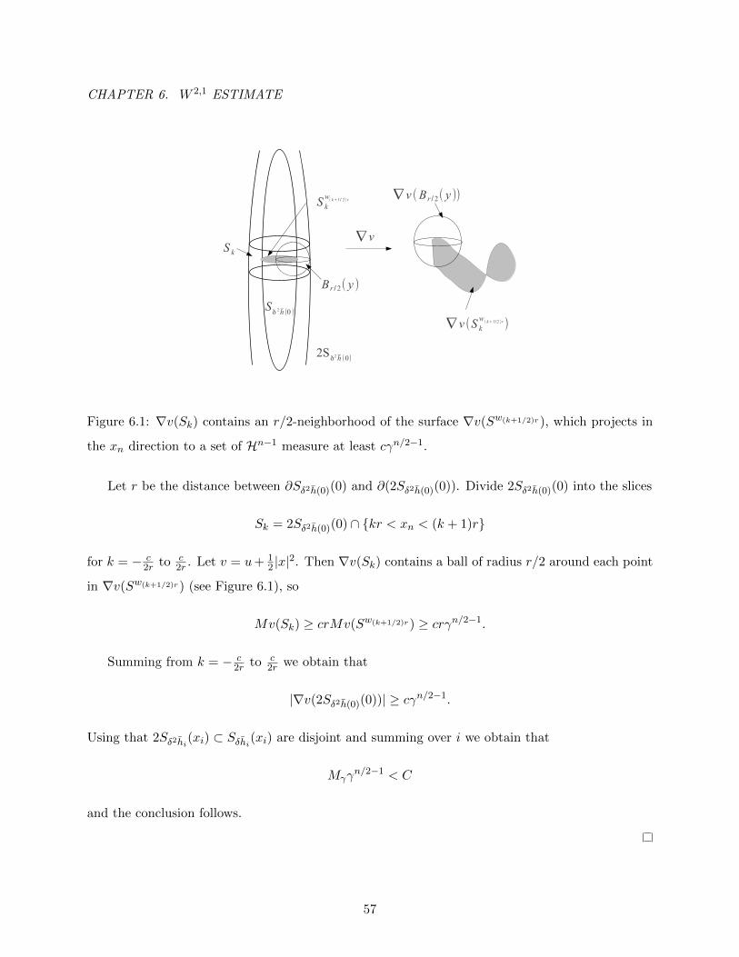
CHAPTER 6. W 2,1 ESTIMATE
S k
S kw
( k+1/ 2) r
∇ v (S kw
( k+1/2 )r )
∇ v
Sδ 2 h (0 )
2Sδ2 h (0)
B r /2( y )
∇ v (B r /2( y ))
Figure 6.1: ∇v(Sk) contains an r/2-neighborhood of the surface ∇v(Sw(k+1/2)r), which projects in
the xn direction to a set of Hn−1 measure at least cγn/2−1.
Let r be the distance between ∂Sδ2h(0)(0) and ∂(2Sδ2h(0)(0)). Divide 2Sδ2h(0)(0) into the slices
Sk = 2Sδ2h(0)(0) ∩ kr < xn < (k + 1)r
for k = − c2r to c
2r . Let v = u+ 12 |x|
2. Then ∇v(Sk) contains a ball of radius r/2 around each point
in ∇v(Sw(k+1/2)r) (see Figure 6.1), so
Mv(Sk) ≥ crMv(Sw(k+1/2)r) ≥ crγn/2−1.
Summing from k = − c2r to c
2r we obtain that
|∇v(2Sδ2h(0)(0))| ≥ cγn/2−1.
Using that 2Sδ2hi(xi) ⊂ Sδhi(xi) are disjoint and summing over i we obtain that
Mγγn/2−1 < C
and the conclusion follows.
57
CHAPTER 6. W 2,1 ESTIMATE
Proof of Theorem 1.4.3. We first consider the set where h(x) ≤ 1t1/2
. At any point in this set,
by Proposition 6.3.1, we can find some r > 0 such that | log r| > c| log t|1/2 and
Mv(Br(x)) > crn−1(log t)η/2.
We conclude that ∫Br(x)
∆u dx ≤ Crn−1 ≤ C
(log t)η/2Mv(Br(x)).
Covering ∆u > t ∩ h(x) ≤ 1t1/2 with these balls and taking a Vitali subcover Bri(xi), we
obtain that ∫∆u>t∩h(x)< 1
t1/2
∆u dx ≤ C
(log t)η/2
∑i
Mv(Bri(xi)) ≤C
(log t)η/2,
giving the desired bound over the “near-singular” points.
We now study the integral of ∆u over the remaining subset of ∆u > t. Take k0 so that
2k0−1 ≤ t1/2 < 2k0 .
Applying Lemma 6.3.4 we obtain that∫∆u>t∩h(x)> 1
t1/2
∆u dx ≤k0∑i=0
∫∆u>t∩F2−i
∆u dx
≤ Ct−εk0∑i=1
2εi
≤ Ct−ε/2,
giving the desired bound.
We next closely examine the geometric properties of maximal sections of solutions in Dn,λ,Λ,K
to prove Proposition 6.3.1.
Let u ∈ Dn,λ,Λ,K and fix x ∈ B1/2. Then for any h > h(x), Sh(x) is not compactly contained in
∂B1. If h(x) > 0, then by Lemma 3.3.2, Sh(x)(x) contains an ellipsoid E centered at x with a long
axis of universal length 2c.
If h(x) = 0 and L is the tangent to u at x then u = L has no extremal points (see chapter 3),
and in particular for any h > 0 we know Sh(x) contains a line segment (independent of h) exiting
∂B1 at both ends.
58
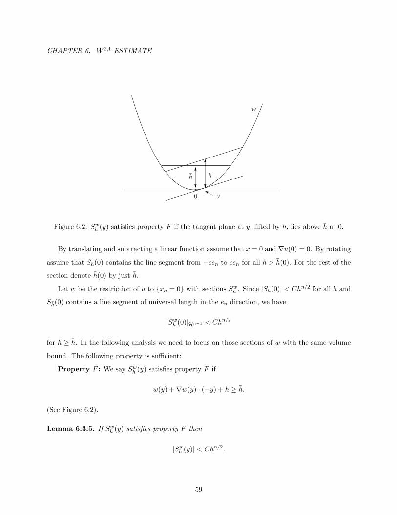
CHAPTER 6. W 2,1 ESTIMATE
h h
y
w
0.
Figure 6.2: Swh (y) satisfies property F if the tangent plane at y, lifted by h, lies above h at 0.
By translating and subtracting a linear function assume that x = 0 and ∇u(0) = 0. By rotating
assume that Sh(0) contains the line segment from −cen to cen for all h > h(0). For the rest of the
section denote h(0) by just h.
Let w be the restriction of u to xn = 0 with sections Swh . Since |Sh(0)| < Chn/2 for all h and
Sh(0) contains a line segment of universal length in the en direction, we have
|Swh (0)|Hn−1 < Chn/2
for h ≥ h. In the following analysis we need to focus on those sections of w with the same volume
bound. The following property is sufficient:
Property F : We say Swh (y) satisfies property F if
w(y) +∇w(y) · (−y) + h ≥ h.
(See Figure 6.2).
Lemma 6.3.5. If Swh (y) satisfies property F then
|Swh (y)| < Chn/2.
59
CHAPTER 6. W 2,1 ESTIMATE
Proof. The plane u(y) +∇u(y) · (z− y) +h is greater than h along z = ten for either t > 0 or t < 0.
Since u < h on the segment from −cen to cen, it follows that Sh(y) contains the line segment from
0 to cen or −cen. Since |Sh(y)| < Chn/2 the conclusion follows.
The first key lemma says that w grows logarithmically faster than quadratic in at least two
directions at a level comparable to h. Let
dy1(h) ≥ dy2(h) ≥ ... ≥ dyn−1(h)
denote the axis lengths of the John ellisoid for Swh (y).
Lemma 6.3.6. For any h > h there exist ε(n), C0 universal, h0 < e−| log h|1/2 and y such that
Swh0(y) satisfies property F and
dyn−2(h0) < C0h1/20 | log h0|−ε.
The next lemma says that if w grows logarithmically faster than quadratic in at least two
directions up to height h then the Monge-Ampere mass of u+ 12 |x|
2 is logarithmically larger than
the mass of ∆u in a ball with radius comparable to h1/2.
Lemma 6.3.7. Fix ε > 0 and assume that for some h > 0, Swh (y) satisfies property F . Then there
exist η1, η2(n, ε) and C depending on universal constants and ε such that if
dyn−2(h) < h1/2| log h|−ε
then for some r < Ch1/2| log h|−η1 we have
M
(u+
1
2|x|2)
(Br(0)) > C−1rn−1| log r|η2 .
These lemmas combine to give the key proposition:
Proof of Proposision 6.3.1: By Lemma 6.3.6, there is some Sh(y) satisfying property F with
dyn−2(h) < C0h1/2| log h|−ε,
with ε(n), C0 universal and h < e−| log(δ+h(x))|1/2 for any δ. The conclusion follows from Lemma
6.3.7.
60
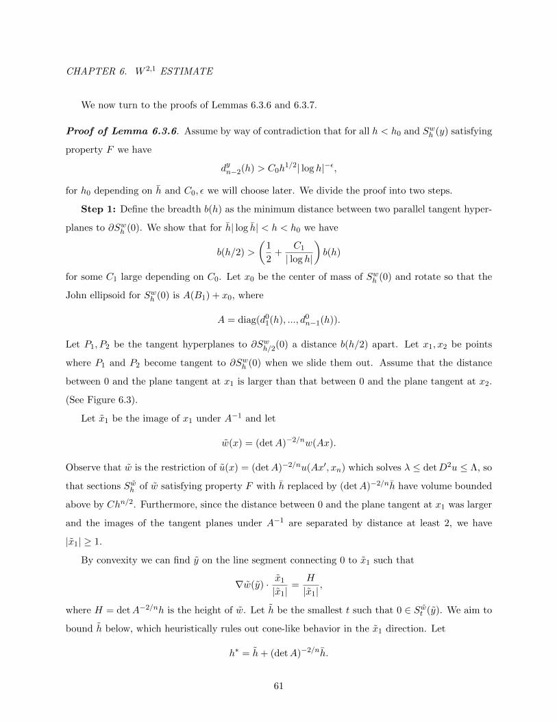
CHAPTER 6. W 2,1 ESTIMATE
We now turn to the proofs of Lemmas 6.3.6 and 6.3.7.
Proof of Lemma 6.3.6. Assume by way of contradiction that for all h < h0 and Swh (y) satisfying
property F we have
dyn−2(h) > C0h1/2| log h|−ε,
for h0 depending on h and C0, ε we will choose later. We divide the proof into two steps.
Step 1: Define the breadth b(h) as the minimum distance between two parallel tangent hyper-
planes to ∂Swh (0). We show that for h| log h| < h < h0 we have
b(h/2) >
(1
2+
C1
| log h|
)b(h)
for some C1 large depending on C0. Let x0 be the center of mass of Swh (0) and rotate so that the
John ellipsoid for Swh (0) is A(B1) + x0, where
A = diag(d01(h), ..., d0
n−1(h)).
Let P1, P2 be the tangent hyperplanes to ∂Swh/2(0) a distance b(h/2) apart. Let x1, x2 be points
where P1 and P2 become tangent to ∂Swh (0) when we slide them out. Assume that the distance
between 0 and the plane tangent at x1 is larger than that between 0 and the plane tangent at x2.
(See Figure 6.3).
Let x1 be the image of x1 under A−1 and let
w(x) = (detA)−2/nw(Ax).
Observe that w is the restriction of u(x) = (detA)−2/nu(Ax′, xn) which solves λ ≤ detD2u ≤ Λ, so
that sections Swh of w satisfying property F with h replaced by (detA)−2/nh have volume bounded
above by Chn/2. Furthermore, since the distance between 0 and the plane tangent at x1 was larger
and the images of the tangent planes under A−1 are separated by distance at least 2, we have
|x1| ≥ 1.
By convexity we can find y on the line segment connecting 0 to x1 such that
∇w(y) · x1
|x1|=
H
|x1|,
where H = detA−2/nh is the height of w. Let h be the smallest t such that 0 ∈ Swt (y). We aim to
bound h below, which heuristically rules out cone-like behavior in the x1 direction. Let
h∗ = h+ (detA)−2/nh.
61
CHAPTER 6. W 2,1 ESTIMATE
x1
x2
b (h /2)
P1
P2
S hw (0)
S h/2w (0) 0.
Figure 6.3:
We have chosen h∗ so that Swh∗(y) and Swδ (y) = A(Swh∗(y)) satisfy property F , where δ = (detA)2/nh∗.
(See Figure 6.4). It follows that
|Swh∗(y)| < C(h∗)n/2.
We now bound the volume of Swh∗(y) by below. Since 0, x1 are in this section, it has diameter
at least 1. Since w has height H it has interior Lipschitz constant CH , so the smallest axis of the
John ellipsoid for Swh∗(y) has length at least ch∗
H . We turn to the remaining axes.
Let Ey be the John ellipsoid for Swδ (y). By contradiction hypothesis for any n− 2 dimensional
plane P passing through the center of Ey, we can find a n − 3 dimensional plane P ′ contained in
P such that P ′ ∩ Ey is an n− 3 dimensional ellipsoid with axes dy1,P ′ ≥ ... ≥ dyn−3,P ′ satisfying
dyn−3,P ′ > C0δ1/2| log δ|−ε.
Take P such that A−1(P ) is perpendicular to the segment connecting 0 and x1. By using the
hypothesis and that w is locally Lipschitz we have
d0n−2(h)d0
n−1(h) > cC0h3/2| log h|−ε.
Since
d01(h)...d0
n−1(h) < Chn2 ,
62
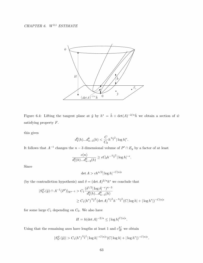
CHAPTER 6. W 2,1 ESTIMATE
w
x1
h
y(det A)−2 /n h
H
. ..0
Figure 6.4: Lifting the tangent plane at y by h∗ = h + det(A)−2/nh we obtain a section of w
satisfying property F .
this gives
d01(h)...d0
n−3(h) <C
C0hn−3
2 | log h|ε.
It follows that A−1 changes the n− 3 dimensional volume of P ′ ∩ Ey by a factor of at least
c(n)
d01(h)...d0
n−3(h)≥ cC0h
−n−32 | log h|−ε.
Since
detA > chn/2| log h|−C(n)ε
(by the contradiction hypothesis) and δ = (detA)2/nh∗ we conclude that
|Swh∗(y) ∩A−1(P ′)|Hn−3 > C1(δ1/2| log δ|−ε)n−3
d01(h)...d0
n−3(h)
≥ C1(h∗)n−3
2 (detA)n−3n h−
n−32 (C| log h|+ | log h∗|)−C(n)ε
for some large C1 depending on C0. We also have
H = h(detA)−2/n ≤ | log h|C(n)ε.
Using that the remaining axes have lengths at least 1 and ch∗
H we obtain
|Swh∗(y)| > C1(h∗)n−1
2 | log h|−C(n)ε(C| log h|+ | log h∗|)−C(n)ε.
63
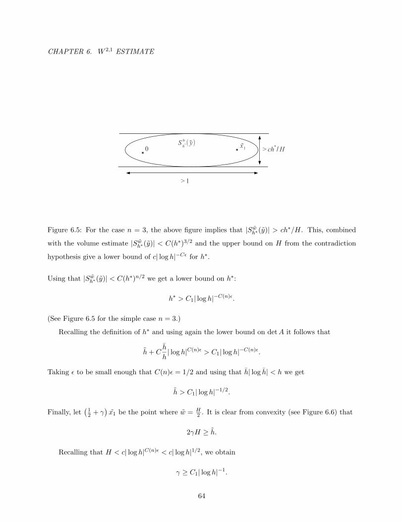
CHAPTER 6. W 2,1 ESTIMATE
Sh*w ( y)
> ch*/Hx1
> 1
0 ..
Figure 6.5: For the case n = 3, the above figure implies that |Swh∗(y)| > ch∗/H. This, combined
with the volume estimate |Swh∗(y)| < C(h∗)3/2 and the upper bound on H from the contradiction
hypothesis give a lower bound of c| log h|−Cε for h∗.
Using that |Swh∗(y)| < C(h∗)n/2 we get a lower bound on h∗:
h∗ > C1| log h|−C(n)ε.
(See Figure 6.5 for the simple case n = 3.)
Recalling the definition of h∗ and using again the lower bound on detA it follows that
h+ Ch
h| log h|C(n)ε > C1| log h|−C(n)ε.
Taking ε to be small enough that C(n)ε = 1/2 and using that h| log h| < h we get
h > C1| log h|−1/2.
Finally, let(
12 + γ
)x1 be the point where w = H
2 . It is clear from convexity (see Figure 6.6) that
2γH ≥ h.
Recalling that H < c| log h|C(n)ε < c| log h|1/2, we obtain
γ ≥ C1| log h|−1.
64
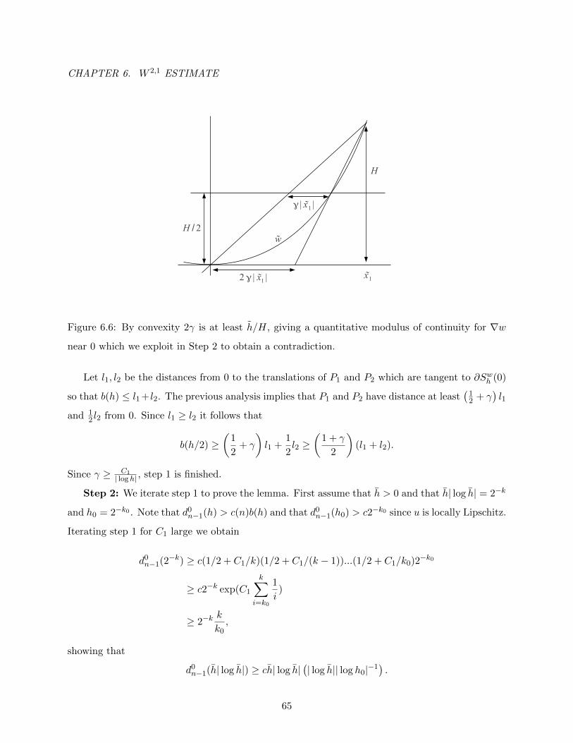
CHAPTER 6. W 2,1 ESTIMATE
γ | x1 |
2 γ | x1 |
w
H
H / 2
x1
Figure 6.6: By convexity 2γ is at least h/H, giving a quantitative modulus of continuity for ∇w
near 0 which we exploit in Step 2 to obtain a contradiction.
Let l1, l2 be the distances from 0 to the translations of P1 and P2 which are tangent to ∂Swh (0)
so that b(h) ≤ l1 + l2. The previous analysis implies that P1 and P2 have distance at least(
12 + γ
)l1
and 12 l2 from 0. Since l1 ≥ l2 it follows that
b(h/2) ≥(
1
2+ γ
)l1 +
1
2l2 ≥
(1 + γ
2
)(l1 + l2).
Since γ ≥ C1| log h| , step 1 is finished.
Step 2: We iterate step 1 to prove the lemma. First assume that h > 0 and that h| log h| = 2−k
and h0 = 2−k0 . Note that d0n−1(h) > c(n)b(h) and that d0
n−1(h0) > c2−k0 since u is locally Lipschitz.
Iterating step 1 for C1 large we obtain
d0n−1(2−k) ≥ c(1/2 + C1/k)(1/2 + C1/(k − 1))...(1/2 + C1/k0)2−k0
≥ c2−k exp(C1
k∑i=k0
1
i)
≥ 2−kk
k0,
showing that
d0n−1(h| log h|) ≥ ch| log h|
(| log h|| log h0|−1
).
65
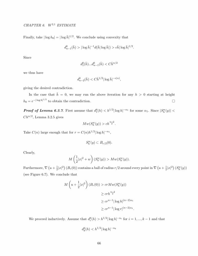
CHAPTER 6. W 2,1 ESTIMATE
Finally, take | log h0| = | log h|1/2. We conclude using convexity that
d0n−1(h) > | log h|−1d(h| log h|) > ch| log h|1/2.
Since
d01(h)...d0
n−1(h) < Chn/2
we thus have
d0n−2(h) < Ch1/2| log h|−ε(n),
giving the desired contradiction.
In the case that h = 0, we may run the above iteration for any h > 0 starting at height
h0 = e−| log h|1/2 to obtain the contradiction.
Proof of Lemma 6.3.7. First assume that dy1(h) < h1/2| log h|−α1 for some α1. Since |Swh (y)| <
Chn/2, Lemma 3.2.5 gives
Mw(Swh (y)) > chn−2
2 .
Take C(n) large enough that for r = C(n)h1/2| log h|−α1 ,
Swh (y) ⊂ Br/2(0).
Clearly,
M
(1
2|x|2 + w
)(Swh (y)) > Mw(Swh (y)).
Furthermore,∇(u+ 1
2 |x|2)
(Br(0)) contains a ball of radius r/2 around every point in∇(u+ 1
2 |x|2)
(Swh (y))
(see Figure 6.7). We conclude that
M
(u+
1
2|x|2)
(Br(0)) > crMw(Swh (y))
≥ crhn−2
2
≥ crn−1| log h|(n−2)α1
≥ crn−1| log r|(n−2)α1 .
We proceed inductively. Assume that dyi (h) > h1/2| log h|−αi for i = 1, ..., k − 1 and that
dyk(h) < h1/2| log h|−αk
66
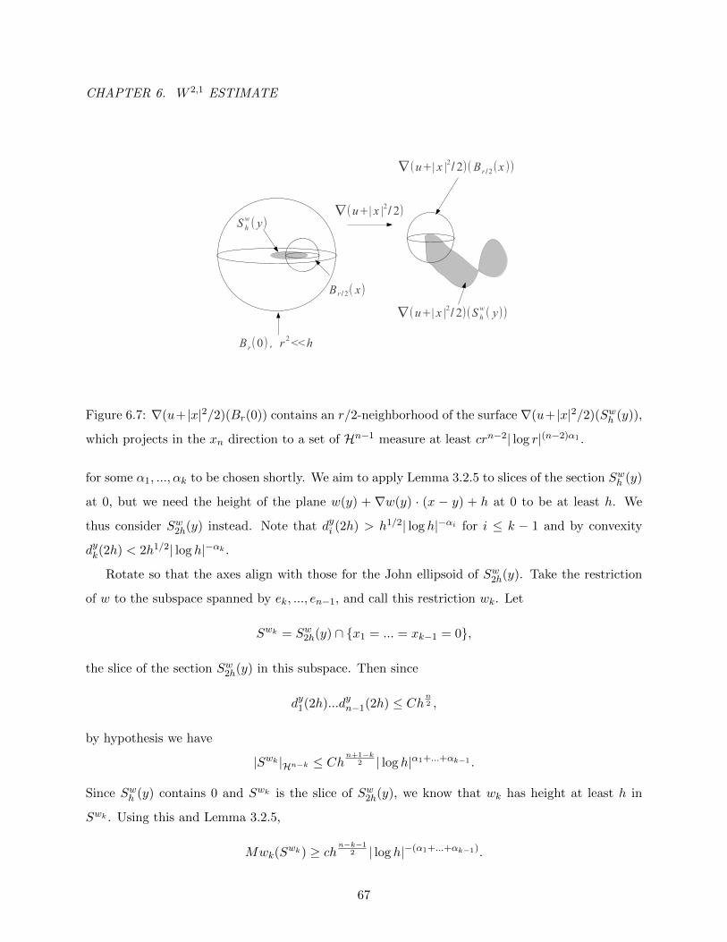
CHAPTER 6. W 2,1 ESTIMATE
B r /2( x)
S hw ( y)
∇(u+| x |2/ 2)
∇(u+| x |2/ 2)(S hw ( y))
∇(u+| x |2/ 2)(B r /2(x ))
B r(0) , r 2 <<h
Figure 6.7: ∇(u+ |x|2/2)(Br(0)) contains an r/2-neighborhood of the surface ∇(u+ |x|2/2)(Swh (y)),
which projects in the xn direction to a set of Hn−1 measure at least crn−2| log r|(n−2)α1 .
for some α1, ..., αk to be chosen shortly. We aim to apply Lemma 3.2.5 to slices of the section Swh (y)
at 0, but we need the height of the plane w(y) + ∇w(y) · (x − y) + h at 0 to be at least h. We
thus consider Sw2h(y) instead. Note that dyi (2h) > h1/2| log h|−αi for i ≤ k − 1 and by convexity
dyk(2h) < 2h1/2| log h|−αk .
Rotate so that the axes align with those for the John ellipsoid of Sw2h(y). Take the restriction
of w to the subspace spanned by ek, ..., en−1, and call this restriction wk. Let
Swk = Sw2h(y) ∩ x1 = ... = xk−1 = 0,
the slice of the section Sw2h(y) in this subspace. Then since
dy1(2h)...dyn−1(2h) ≤ Chn2 ,
by hypothesis we have
|Swk |Hn−k ≤ Chn+1−k
2 | log h|α1+...+αk−1 .
Since Swh (y) contains 0 and Swk is the slice of Sw2h(y), we know that wk has height at least h in
Swk . Using this and Lemma 3.2.5,
Mwk(Swk) ≥ ch
n−k−12 | log h|−(α1+...+αk−1).
67
CHAPTER 6. W 2,1 ESTIMATE
Finally, take C(n) large enough that for r = C(n)h1/2| log h|−αk we have
Swk ⊂ Br/2(0).
By strict quadratic growth, ∇(u+ 1
2 |x|2)
(Br(0)) contains a ball of radius r/2 around every point
in ∇(u+ 12 |x|
2)(Swk). It follows that
M
(u+
1
2|x|2)
(Br(0)) ≥ cMwk(Swk)rk
≥ chn−k−1
2 | log h|−(α1+...+αk−1)rk
≥ crn−1| log r|(n−k−1)αk−(α1+...+αk−1).
Choose βi so that (n − k − 1)βk − (β1 + ... + βk−1) = 1 and let αi = cβi, with c chosen so that
αn−2 = ε. If dy1(h) < h1/2| log h|−α1 , we are done by the first step, so assume not. Then apply the
inductive step for i = 2, ..., n− 2 to conclude the proof.
6.4 Example showing optimality of Theorem 1.4.3
In this section we construct a solution to detD2u = 1 in R3 with a singular set of Hausdorff
dimension exactly 2. A small modification gives the analagous example in Rn with a singular set
of Hausdorff dimension n − 1. This shows that the estimate on the Hausdorff dimension of the
singular set in chapter 4 cannot be improved to n− 1− δ for any δ.
We then show that the second derivatives of this solution are not in L logM L for M large,
showing that theorem 1.4.3 is optimal.
We proceed in several steps:
1. The key step is to construct a subsolution w in R3 satisfying detD2w ≥ 1 that degenerates
along x1 = x2 = 0 and grows logarithmically faster than quadratic in the x1 direction, in
particular like x21| log x1|4.
2. Next, we construct S ⊂ [−1, 1] of Hausdorff dimension 1 and a convex function v on [−1, 1]
such that v separates from its tangent line faster than r2| log r|4 at each point in S.
3. Finally, we obtain our example by solving the Dirichlet problem
detD2u = 1 in Ω = |x′| < 1 × (−1, 1), u|∂Ω = C(v(x1) + |x2|)
68
CHAPTER 6. W 2,1 ESTIMATE
and comparing with w at points in S × 0 × ±1.
In the following analysis c, C will denote small and large constants respectively.
Construction of w: We first seek a function with just faster than quadratic growth in one
direction and sections Sh(0) with volume smaller than h3/2. To that end, let
g(x1, x2) = x21| log x1|α +
|x2|| log x2|β
for some α, β to be chosen shortly. It is tempting to guess w = g(x1, x2)(1 + x23). However, the
dominant terms in the determinant of the Hessian near the x2 axis are
| log x1|α
| log x2|2β
(1
| log g|− x2
3
),
where the first comes from the diagonal entries and the second from the mixed derivatives. Thus,
this function is not convex. This motivates the following modification:
w(x′, x3) = g(x′)
(1 +
x23
| log g(x′)|
).
It is straightforward to check that the leading terms in the determinant of the Hessian (taking x3
small) arex2
1| log x1|2α
|x2(log x2)β+1 log g|+
| log x1|α
|(log x2)1+2β log g|,
since now the mixed derivative terms have the same homogeneity in log(g) as the diagonal terms.
For |x′| small, the first term is large in |x2| < |x1|3, and by taking α = 2 + 2β the second term is
bounded below by a positive constant in |x2| ≥ |x1|3. Thus, up to rescaling and multiplying by
a constant we have
detD2w ≥ 1
in Ω = |x′| < 1 × (−1, 1). For convenience, we take β = 1 and α = 4 for the rest of the example.
Construction of S: Start with the interval [−1/2, 1/2]. For the first step remove an open
interval of length 56 from the center. At the kth step, remove intervals a fraction 5
k+5 of the length
of the remaining 2k intervals from their centers. Denote the centers of the removed intervals by
xi,k2k
i=1, and the intervals by Ii,k. Finally, let
S = [−1, 1]− ∪i,kIi,k.
69
CHAPTER 6. W 2,1 ESTIMATE
Let lk = |Ii,k|. It is easy to check
lk =10
k + 52−k
(1− 5
k + 4
)...
(1− 5
6
)≤ C
k62−k.
One checks similarly that the length of the remaining intervals after the kth step is at least
2−kk−15.
It follows that
inf
∞∑i=1
ri| log(ri)|15 : Bri(xi) cover S, ri < δ
> c (6.3)
for all δ > 0. In particular, the Hausdorff dimension of S is exactly 1.
Construction of v: Let
f(x) =
|x| |x| ≤ 1
2|x| − 1 |x| > 1
We add rescalings of f together to produce the desired function:
v(x) =
∞∑k=1
k4l2kf(l−1k (x− xi,k)).
We now check that v satisfies the desired properties:
1. v is convex, as the sum of convex functions. Furthermore, using that lk < C2−kk−6 we have
|v(x)| ≤ C∞∑k=1
2k∑i=1
k4lk
≤ C∞∑k=1
k−2
≤ C
so v is bounded.
2. Let x ∈ S. We aim to show that v separates from a tangent line more than r2| log(r)|4 a
distance r from x. By subtracting a line assume that v(x) = 0 and that 0 is a subgradient at
x. Assume further that x+ r < 1/2 and that lk < r ≤ lk−1. There are two cases to examine:
70
CHAPTER 6. W 2,1 ESTIMATE
Case 1: There is some y ∈ (x+ r/2, x+ r) ∩ S. Then by the construction of S it is easy to
see that there is some interval Ii,k such that Ii,k ⊂ (x, x+ r). On this interval, v grows by
k4l2k ≥ cl2k| log(lk)|4 ≥ cr2| log(r)|4.
Case 2: Otherwise, there is an interval Ii,j of length exceeding r/2 such that (x+r/2, x+r) ⊂
Ii,j . Then at the left point of Ii,j , the slope of v jumps by at least k4lk. It follows that at
x+ r, v is at least
crk4lk ≥ cr2| log(r)|4.
Thus, v has the desired properties.
Construction of u: Let ϕ(x1, x2, x3) = C(v(x1)+ |x2|) for a constant C we will choose shortly,
and obtain u by solving the Dirichlet problem
detD2u = 1 in Ω = |x′| < 1 × [−1, 1], u|∂Ω = ϕ.
Take x ∈ S × 0 × ±1. By translating and subtracting a linear function assume that x1 = 0
and 0 is a subgradient for ϕ at x. Taking C large we guarantee that
ϕ(x1, x2,±1) > C(x21| log(x1)|4 + |x2|) > w(x1, x2,±1)
for all x1, x2, and that that ϕ > w on the sides of Ω. Thus, u ≥ w in all of Ω. Since u = 0 at both
(0, 0,±1) and w(0, 0, x3) = 0 for all |x3| < 1, we have by convexity that u = 0 along (0, 0, x3).
This shows that for these examples
Σ ⊂ S × 0 × (−1, 1),
which has Hausdorff dimension exactly 2.
Remark 6.4.1. To get the analagous example in Rn, take
u(x1, x2, x3) + x24 + ...+ x2
n.
71
CHAPTER 6. W 2,1 ESTIMATE
We now examine the integrability of the second derivatives for the singular solution constructed
above. In chapter 4 we construct, for any ε, solutions to detD2u = 1 in Rn that are not in W 2,1+ε,
but as ε→ 0 these examples blow up. We aim to improve this by showing that the example above
is not in W 2,1+ε for any ε, and in fact the second derivatives are not in L logM L for M large.
Let φ(x) = (1 + x)(log(1 + x))M for some M large. Then φ is convex for x ≥ 0, so for any
nonnegative integrable function f and ball Br we have by Jensen’s inequality that∫Br
φ(rnf(x)) dx ≥ crnφ(∫
Br
f(x) dx
).
Taking f(x) = r−n∆u(x) we obtain∫Br
(1 + ∆u)(log(1 + ∆u))M dx ≥ c(∫
Br
∆u dx
)(log
(r−n
∫Br
∆u dx
))M.
Recall that at points x ∈ S × 0 × (−1, 1)n−2 the subsolutions w touch u by below, and that w
grows like |x2|| log x2|−1 at x. It follows that
sup∂Br(x)
(u− u(x)) ≥ cr| log r|−1.
Applying convexity we conclude that
∫Br(x)
(1 + ∆u) (log(1 + ∆u))M dx ≥ c
(∫∂Br(x)
uν
)(log
(r−n
∫∂Br(x)
uν
))M≥ crn−1| log r|−1
(log(cr−1| log(r)|−1)
)M≥ crn−1| log r|M−1.
Cover Σ ∩B1/2 with balls of radius less than δ and take a Vitali subcover BriNi=1. We then have
∫B1/2
(1 + ∆u) (log(1 + ∆u))M dx ≥ cN∑i=1
rn−1i | log ri|M−1,
and for M large the right side goes to ∞ as δ → 0 by equation 6.3.
Thus, the second derivatives of u are not in L logM L for M large, and in particular u is not in
W 2,1+ε for any ε > 0.
72
BIBLIOGRAPHY
Bibliography
[A] Alberti, G. On the structure of singular sets of convex functions. Calc. Var. Partial Differ-ential Equations 2 (1994), no. 1, 17-27.
[AAC] Alberti, G.; Ambrosio, L.; Cannarsa, P. On the singularities of convex functions.Manuscripta Math. 76 (1992), no. 3-4, 421-435.
[Al] Alexandrov, A. D. Smoothness of the convex surface of bounded Gaussian curvature. C. R.(Doklady) Acad. Sci. URSS (N. S.) 36 (1942), 195-199.
[AS] Armstrong, S.; Silvestre, L. Unique continuation for fully nonlinear elliptic equations. Math.Res. Lett. 18 (2011), no. 5, 921-926.
[B] Brenier, Y. Polar factorization and monotone rearrangement of vector-valued functions.Comm. Pure Appl. Math. 44 (1991), no. 4, 375-417.
[C1] Caffarelli, L. A localization property of viscosity solutions to the Monge-Ampere equationand their strict convexity. Ann. of Math. 131 (1990), 129-134.
[C2] Caffarelli, L. Interior W 2,p estimates for solutions of Monge-Ampere equation. Ann. of Math.131 (1990), 135-150.
[C3] Caffarelli, L. A note on the degeneracy of convex solutions to the Monge-Ampere equation.Comm. Partial Differential Equations 18 (1993), 1213-1217.
[CC] Caffarelli, L.; Cabre, X. Fully Nonlinear Elliptic Equations. Colloquium Publications 43.Providence, RI: American Mathematical Society (1995).
[CG] Caffarelli, L.; Gutierrez, C. Properties of solutions of the linearized Monge-Ampere equation.Amer. J. Math 119 (1997), 423-465.
[CNS] Caffarelli L.; Nirenberg, L.; Spruck, J. Dirichlet problem for nonlinear second order ellipticequations I, Monge-Ampere equations. Comm. Pure Appl. Math. 37 (1984), 369-402.
[Cal] Calabi, E. Improper affine hyperspheres of convex type and a generalization of a theoremby K. Jorgens. Michigan Math. J. 5 (1958), 105-126.
[DF] De Philippis, G.; Figalli, A. W 2,1 regularity for solutions of the Monge-Ampere equation.Invent. Math. 192 (2013), 55-69.
73
BIBLIOGRAPHY
[DFS] De Philippis, G.; Figalli, A.; Savin, O. A note on interior W 2,1+ε estimates for the Monge-Ampere equation. Math. Ann. 357 (2013), 11-22.
[GL] Garofalo, N. ; Lin, F. H. Unique continuation for elliptic operators: a geometric-variationalapproach. Comm. Pure Appl. Math. 40 (1987), no. 3, 347-366.
[Gut] Gutierrez, C. “The Monge-Ampere Equation,” Progress in Nonlinear Differential Equationsand their Applications 44, Birkhauser Boston, Inc., Boston, MA, 2001.
[Har] Hartenstine, D. The dirichlet problem for the Monge-Ampere equation in convex (but notstrictly convex) domains. Electron. J. Differential Equations (2006), No. 138, 1-9.
[H] Hormander, L. The Analysis of Linear Partial Differential Operators III, PseudodifferentialOperators. Grundlehren der Mathematischen Wissenschaften, 274. Springer-Verlag, Berlin,1985.
[Mi] Miller, K. Nonunique continuation for uniformly parabolic and elliptic equations in self-adjoint divergence form with Holder continuous coefficients. Arch. Rational Mech. Anal. 54(1974), 105-117.
[M1] Mooney, C. Partial regularity for singular solutions to the Monge-Ampere equation. Comm.Pure Appl. Math, to appear.
[M2] Mooney, C. W 2,1 estimate for singular solutions to the Monge-Ampere equation. Ann. Sc.Norm. Sup. Pisa Cl. Sc., to appear.
[Pl] Plis, A. On non-uniqueness in Cauchy problem for an elliptic second order differential oper-ator. Bull. Acad. Polon. Sci. 11 (1963), 95-100.
[P] Pogorelov, A. The regularity of the generalized solutions of the equation det(
∂2u∂xi∂xj
)=
ϕ(x1, x2, ..., xn) > 0. (Russian) Dokl. Akad. Nauk SSSR 200 (1971), 534-537.
[S] Savin, O. Small perturbation solutions to elliptic equations. Comm. Partial DifferentialEquations 32 (2007), no. 4-6, 557-578.
[W] Wang, X. J. Regularity for Monge-Ampere equation near the boundary. Analysis 16 (1996)101-107.
74


![Multigrid for Elliptic Monge Amp ere Equation · Multigrid for Elliptic Monge Amp ere ... Monge-Amp ere equations were rst studied by Gaspard Monge in 1784 [3] and later by Andre-Marie](https://img.pdfslide.us/doc/110x75/5c45b40693f3c34c50612fad/multigrid-for-elliptic-monge-amp-ere-equation-multigrid-for-elliptic-monge-amp.jpg)

![a priori arXiv:1212.5617v1 [math.AP] 21 Dec 2012 · Monge-Amp ere equation, singular perturbation, vanishing moment method, con- ... put the vanishing moment method on a solid footing](https://img.pdfslide.us/doc/110x75/5e3fae42dc1e8a24ee2c5205/a-priori-arxiv12125617v1-mathap-21-dec-2012-monge-amp-ere-equation-singular.jpg)


![Analytic Methods in Algebraic Geometrydemailly/...4 Analytic Methods in Algebraic Geometry [Dem93b], obtained by means of analytic techniques and Monge-Amp`ere equations with isolated](https://img.pdfslide.us/doc/110x75/5ed5e855f6ea6c673b148dc1/analytic-methods-in-algebraic-geometry-demailly-4-analytic-methods-in-algebraic.jpg)