BIT manuscript No.(will be inserted by the editor)

Spline element method for Monge-Ampere equations

Gerard Awanou

Received: date / Accepted: date

Abstract We analyze the convergence of an iterative method for solving thenonlinear system resulting from a natural discretization of the Monge-Ampereequation with smooth approximations. We make the assumption, supportedby numerical experiments for the two dimensional problem, that the discreteproblem has a convex solution. The method we analyze is the discrete ver-sion of Newton’s method in the vanishing moment methodology. Numericalexperiments are given in the framework of the spline element method.

Keywords iterative methods · Monge-Ampere · C1 conforming approxima-tions

Mathematics Subject Classification (2000) 65N30 · 35J25

1 Introduction

This paper addresses the numerical solution of the Dirichlet problem for theMonge-Ampere equation

detD2u = f inΩ, u = g on ∂Ω. (1)

Here D2u =

((∂2u)/(∂xi∂xj)

)i,j=1,...,n

is the Hessian of u and f, g are given

functions with f ≥ c0 > 0 for a constant c0. The domain Ω ⊂ Rn, n = 2, 3is assumed to be bounded and convex with a polygonal boundary and ∂Ωdenotes its boundary.

Gerard AwanouDepartment of Mathematics, Statistics, and Computer Science (M/C 249), University ofIllinois at Chicago, Chicago, IL, 60607-7045Tel.: +1-312-413-2167Fax: +1-312-996-1491E-mail: awanou@uic.edu

2 Gerard Awanou

Let Vh denote a finite dimensional space of C1 functions which are piecewisepolynomials of degree d at least 2, and let us assume that f ∈ L1(Ω). Weconsider the discrete problem: find uh ∈ Vh such that∫

Ω

vh detD2uh dx =

∫Ω

fvh dx,∀vh ∈ Vh ∩H10 (Ω)

uh = ghon ∂Ω,

(2)

where gh is the natural interpolant in Vh of a smooth extension of g. In thispaper, we make the assumption that (2) has a strictly convex solution uh.We analyze the convergence of the following iterative method. Given an initialguess u0h ∈ Vh with u0h = gh on ∂Ω, find uk+1

h ∈ Vh such that uk+1h = gh on ∂Ω

and such that for ε > 0 we have ∀vh ∈ Vh ∩H10 (Ω)

ε

∫Ω

∆uk+1h ∆vh dx+

∫Ω

[(cof D2ukh)Duk+1h ] ·Dvh dx = −

∫Ω

fvh dx

+ ε3∫∂Ω

∂vh∂n∂Ω

ds+n− 1

n

∫Ω

[(cof D2ukh)Dukh] ·Dvh dx.(3)

We use the notation Dv to denote the gradient vector of the function v andrecall that cof A denotes the matrix of cofactors of the matrix A. The maindifficulties of the numerical resolution of (1) is that when it does not have asmooth solution, Newton’s method (i.e. (3) with ε = 0) breaks down.

In [5] we show that (2) is well defined and has a strictly convex solutionwhen (1) has a smooth strictly convex solution. Less restrictive conditionsunder which (2) has a strictly convex solution are addressed in [6] in theframework of the Aleksandrov theory of the Monge-Ampere equation. Theassumption of existence of a strictly convex solution of (2) is supported in thispaper by numerical experiments in two dimension. We prove the convergenceof the iterations (3) to a limit uε,h which solves a discrete variational problem.With that result, one may prove a quadratic convergence rate for (3) as aniterative method converging to uε,h, using for example the techniques of [5].That issue is not addressed in this paper since (3) is not a direct method forsolving (2).

For C1 conforming approximations, we use the spline element method [2,8,9,13,37,3]. It uses piecewise polynomials of arbitrary degree and Lagrangemultipliers to enforce continuity and smoothness conditions as well as con-straints. However, unlike other methods which also use Lagrange multipliers,the constraints here are enforced exactly. More details are given in Section 4.1.An alternative to the spline element method is the Argyris finite element forthe two dimensional problem or concepts from isogeometric analysis [50]. Thestudy of C1 conforming approximations provides a natural setting for presen-ting techniques for proving results on the numerical analysis of Monge-Ampereequations. These techniques may be extended to the setting of isogeometricanalysis, mixed finite elements, Lagrange elements or the standard finite dif-ference method.

Methods for Monge-Ampere equation 3

1.1 Relation with other work

The first rigorous treatment of the numerical resolution of the Monge-Ampereequation was given in [46]. See also the references therein for some heuristicarguments previously proposed for the balance equation of dynamic meteo-rology, a Monge-Ampere type equation. The work of Oliker and Prussner in[46] is based on the notion of weak solution of (1) in the sense of Aleksan-drov. Dean and Glowinski [23–25,34] suggested that the numerical resolutionof (1), for the notion of weak solution in the viscosity sense, can be approachedthrough standard discretizations of the finite element or finite difference type.It is known [35] that the notions of viscosity and Aleksandrov solutions of(1) are equivalent for f > 0 and continuous on Ω. The analysis of numericalmethods for (1) under the assumption that the solution is smooth was firstinitiated in [17,15,18,19]. In particular, Bohmer analyzed the discretization(2). Bohmer proved the quadratic convergence of Newton’s method for solving(2), [15, Theorem 9.1] and his method has been implemented only recently[22]. Oberman in [45] constructed finite difference schemes which satisfy theconditions of monotonicity, stability and consistency of convergence of nume-rical schemes to viscosity solutions. His approach through viscosity solutionswas later generalized in [31,33]. Feng and Neilan proposed the notion of vani-shing moment methodology [27,29,30,41]. The latter has been recently shownto be valid for strictly convex radial viscosity solutions [26]. The formal limitof the vanishing moment methodology turns out, in the case of the Monge-Ampere equation, to be the method recently proposed by Lakkis and Pryer in[39]. Neilan analyzed the method of Lakkis and Pryer for the two-dimensionalproblem under the assumption that the solution is smooth in [42]. Awanouand Li provided a unified analysis for both dimensions from a different pointof view in [10]. Several other numerical methods for (1) have been proposed,e.g. by Mohammadi [40] and by Zheligovsky et al [51].

In [5,1,6,4] we started the study of the numerical resolution of (1) fromthe point of view of compatible discretizations. Our point of view is that,after regularization of the data, the discretization of (1) leads to a sequence ofdiscrete problems, the solution of which are discrete strictly convex functions ina sense that has to be defined for each type of discretization. For (2), the notionof convexity used in [5] is the usual notion of convexity while in [1] we requiredthe approximations to be piecewise strictly convex. For another example, in[4] for the (non monotone) standard finite discretization, we required a certaindiscrete Hessian to be positive definite. Our approach is detailed in [6] andis based on the notion of Aleksandrov solution of (1), the characterization ofAleksandrov solution based on approximation by smooth functions [49], andthe technique of considering a smooth uniformly convex exhaustion of thedomain. The conclusion is that for the numerical analysis of robust methodsfor (1), one only needs to understand how the methods perform when (1) isassumed to have a smooth strictly convex solution.

To the best of our knowledge the theoretical convergence, even for smoothsolutions, of the methods proposed by Dean and Glowinski, Mohammadi, and

4 Gerard Awanou

Zheligovsky, is not understood. It is also not known whether the vanishingmoment methodology approach is valid for non radial viscosity solutions of(1). We propose to analyze these methods from the new point of view weembraced in [5,1,6,4]. The goal is thus to understand how these methodsperform when (1) is assumed to have a strictly convex smooth solution. Thereare several motivations for pursuing this line of investigation. For example,the method of Mohammadi is known to be robust even when the right handside f is not positive. The vanishing moment methodology allows to use aNewton type iterative method for the resolution of (2). Although this featureis shared with the mixed method approach, a complete understanding of thevanishing moment methodology could lead to the development of even morerobust algorithms. We recall that the vanishing moment methodology consistsin the singular perturbation problem

−ε∆2uε + det D2uε = f, in Ω, uε = g, ∆uε = ε2 on ∂Ω, ε > 0. (4)

In [27,29,30,41], it was assumed that if f > 0, (4) has a unique strictly convexsolution uε and uε converges uniformly on Ω to the unique convex viscositysolution of (1). Moreover, it was assumed that

||uε||j = O(ε−j−12 ), j = 2, 3; ||uε||2,∞ = O(ε−1)

|| cof D2uε||∞ = O(ε−1); ||(D2uε)i,j ||0 = O(ε−12 ), i, j = 1, . . . , n.

(5)

In (5), we used standard Sobolev norms notation recalled in section 2. Werecall that the above assumptions were proved for radial solutions in [26]. Asa consequence of these assumptions, the problem: find uε,h ∈ Vh such thatuε,h = gh on ∂Ω and for all vh ∈ Vh ∩H1

0 (Ω),

ε

∫Ω

∆uε,h∆vh dx−∫Ω

(detD2uε,h)vh dx = −∫Ω

fvh dx+ ε3∫∂Ω

∂vh∂n∂Ω

ds,

(6)

can be shown to be well posed and error estimates were derived. Feng andNeilan mentioned the convexity of uε,h as a major open problem, [28, Remark3.2].

It is not very difficult to see that if one replaces the nonlinear operatordet in (4) by the Laplace operator, one obtains a singular perturbation prob-lem similar to the one analyzed in [44]. It is therefore reasonable to expectthat the techniques in [44] can be extended to the vanishing moment metho-dology. Since the ultimate goal of the methodology is to produce numericalapproximations for (1), we analyze in this paper directly the iterative method(3) which is Newton’s method applied to problem (6). It turns out that atthe discrete level the strategies used in [44, Lemma 5.1] take a simpler form.We wish to address the proof of the assumptions made in [27,29,30,41] inthe framework of the Aleksandrov theory of the Monge-Ampere equation [6],taking into account the above remarks, in a separate work.

The contributions of this paper are therefore

Methods for Monge-Ampere equation 5

– the validation of the vanishing moment methodology for the numericalresolution of (1), an issue which has been open for more than 7 years, ifone takes into account the work in [6]. It validates the method for smoothnot necessarily radial solutions if one takes only into account the work in[5] or alternatively the work of Bohmer [15]

– the convexity of the numerical solution in the vanishing moment methodo-logy is established

– an increase in the understanding of numerical methods for Monge-Amperetype equations. In particular this paper links the vanishing moment me-thodology to the unifying point of view presented in [5,1,6,4].

The interested reader may recover, using the strategies of this paper, the resultsof [29] from the ones in [42,10]. The analysis for non smooth solutions of themixed methods discussed in [39,43,10] will be discussed in [7].

1.2 Organization of the paper

The paper is organized as follows: in the second section, we introduce somenotation and give some preliminary results. In section 3 we prove the conver-gence of Newton’s method in the vanishing moment methodology. The lastsection is devoted to numerical experiments.

2 Notation and Preliminaries

We use the usual notation Lp(Ω), 1 ≤ p ≤ ∞ for the Lebesgue spaces andW k,p(Ω) for the Sobolev spaces with norms ||.||k,p and semi-norm |.|k,p. Inparticular, Hk(Ω) = W k,2(Ω) and in this case, the norm and semi-norms willbe denoted respectively by ||.||k and |.|k. For two n×n matrices A,B, we recallthe Frobenius inner product A : B =

∑ni,j=1AijBij , where Aij and Bij refer

to the entries of the corresponding matrices. For a matrix field A, we denoteby divA the vector obtained by taking the divergence of each row. We will usethe notation

||A||∞ := maxi,j|aij |,

for a matrix A = (aij)i,j=1,...,n and denote by n∂Ω the unit outward normalvector to ∂Ω. We make the usual convention of denoting constants by C. Ourresults hold for h sufficiently small. We will thus state them for h ≤ h0 ≤ 1where h0 is a constant which may change from occurrences.

We require our approximation spaces Vh to satisfy the following property:there exists an interpolation operator Ih mapping W l+1,p(Ω) into the spaceVh for 1 ≤ p ≤ ∞, 0 ≤ l ≤ d such that

||v − Ihv||k,p ≤ Chl+1−k||v||l+1,p, (7)

for 0 ≤ k ≤ l and the inverse estimates

||v||s,p ≤ Chl−s+min(0,np−nq )||v||l,q,∀v ∈ Vh, (8)

6 Gerard Awanou

and for 0 ≤ l ≤ s, 1 ≤ p, q ≤ ∞.The above assumptions are known to be satisfied for standard finite element

spaces [20]. For the spline spaces used in the computations, (7) is known tohold [38]. One may view (8) as a consequence of Markov inequality, [38, p. 2],and [16, section 4.2.6] for details.

It follows from (7) that

||Ihv||k,p ≤ C||v||k,p,

for 1 ≤ p ≤ ∞ and 0 ≤ k ≤ d.We will need the following lemma whose proof can be found in [5].

Lemma 1 We have

detD2v =1

n(cof D2v) : D2v =

1

ndiv((cof D2v)Dv

).

And for F (v) = detD2v we have

F ′(v)(w) = (cof D2v) : D2w = div((cof D2v)Dw

),

for v, w sufficiently smooth.

Let us denote by λ1(D2v) and λn(D2v) the smallest and largest eigenvalues re-spectively of D2v, for v piecewise smooth. We make in this paper the followingassumption

Assumption 1 We assume that (2) has a strictly convex solution uh with 0 <2C0 ≤ λ1(D2uh) ≤ λn(D2uh) ≤ C00/2 for constants C0 and C00 independentof h.

We define for ρ > 0

Bρ(uh) = vh ∈ Vh, ||vh − uh||1 ≤ ρ ,

and we have

Lemma 2 Under Assumption 1, there exists a constant Cconv such that forρ ≤ Cconvh

1+n/2 and for vh ∈ Bρ(uh), vh is strictly convex with λ1(D2vh) ≥C0.

Proof By the continuity of the eigenvalues of a (symmetric) matrix as a func-tion of its entries, [48] Appendix K, or [36], there exists δ > 0 such that for|vh − uh|2,∞ ≤ δ we have |λ1(D2vh(x))− λ1(D2uh(x))| < C0 for all x ∈ Ω.

By the inverse estimate (8), we have |vh−uh|2,∞ ≤ Cinvh−1−n/2||vh−uh||1.Thus taking Cconv = δ/(2Cinv) we obtain for ||vh − uh||1 ≤ Cconvh

1+n/2, weget for all x ∈ Ω, |λ1(D2vh(x)) ≥ λ1(D2uh(x))−C0 ≥ C0. Since vh is piecewiseconvex and vh ∈ C1(Ω), vh is convex, [21, section 5]. This completes the proof.

Arguing as in the proof of Lemma 2, one shows that if the exact smoothsolution u of (1) is strictly convex, i.e. for f ≥ c0 > 0, then Ihu is also strictlyconvex and the solution uh of (2) is also strictly convex. See [5] for details.

Methods for Monge-Ampere equation 7

3 Convergence of the discrete vanishing moment methodology

In this section, we make the assumption that

ρ ≤ Cconvh1+n/2.

By Lemma 1, we have for wh ∈ Bρ(uh) and vh ∈ Vh ∩H10 (Ω),∫

Ω

[(cof D2wh)Dwh] ·Dvh dx = −∫Ω

div[(cof D2wh)Dwh]vh dx

= −n∫Ω

(detD2wh)vh dx.

(9)

Thus, we can rewrite (3) as

ε

∫Ω

∆uk+1h ∆vh dx+

∫Ω

[(cof D2ukh)Duk+1h ] ·Dvh dx = ε3

∫∂Ω

∂vh∂n∂Ω

ds

+

∫Ω

pkhvh dx,

(10)

for all vh ∈ Vh ∩H10 (Ω) with

pkh = −f − (n− 1) detD2ukh.

Given ukh ∈ Bρ(uh), with ukh = gh on ∂Ω, let uk+1h satisfy uk+1

h = gh on∂Ω and for all vh ∈ Vh ∩H1

0 (Ω),∫Ω

[(cof D2ukh)Duk+1h ] ·Dvh dx =

∫Ω

pkhvh dx. (11)

We note that since ukh is strictly convex, the existence of uk+1h follows from

the Lax-Milgram lemma. The following theorem identifies uk+1h as the result

of one step of Newton’s method applied to (2) starting with ukh.

Theorem 1 Given ukh ∈ Bρ(uh), ρ ≤ Cconvh1+n/2, the solution uk+1

h of (11)solves∫

Ω

[div((cof D2ukh)D(uk+1h − ukh)]vh dx = −

∫Ω

(detD2ukh − f)vh dx

uk+1h = ghon ∂Ω,

(12)

∀vh ∈ Vh ∩H10 (Ω). Moreover there exists h0 ≤ 1 such that for h ≤ h0

||uk+1h − uh||1 ≤ C||ukh − uh||21. (13)

8 Gerard Awanou

Proof The result follows from integration by parts and taking into account (9).Explicitly, using the expression of the Frechet derivative of the determinant ofLemma 1, we obtain (12) as one step of Newton’s method applied to (2). Wethen obtain by an integration by parts

−∫Ω

[(cof D2ukh)Duk+1h ] ·Dvh dx+

∫Ω

[(cof D2ukh)Dukh] ·Dvh dx

= −∫Ω

(detD2ukh − f)vh dx.

By (9), we obtain

−∫Ω

[(cof D2ukh)Duk+1h ] ·Dvh dx− n

∫Ω

(detD2ukh)vh dx

= −∫Ω

(detD2ukh − f)vh dx,

from which (11) follows.The inequality (13) is nothing but a consequence of a Newton’s step for

C1 conforming approximations of the Monge-Ampere equation. The quadraticconvergence rate of Newton’s method follows for example from [15, Theorem9.1]. For the two dimensional problem, (13) can also be inferred from [43].

Remark 1 In a more general setting, we analyzed in [5] the pseudo-transientiterative method, one step of which, starting with ukh, is given by

−ν∫Ω

(Duk+1h −Dukh) ·Dvh dx

+

∫Ω

[div((cof D2ukh)D(uk+1h − ukh)]vh dx = −

∫Ω

(detD2ukh − f)vh dx

uk+1h = ghon ∂Ω,

for ν ≥ 0. For ν = 0, we recover one step of Newton’s method, the quadraticconvergence rate of which follows from [5, 3.10]. See [5, Remark 3.2]. In bothcases discussed above, the rate of convergence is mesh dependent. In particular,[5, Remark 3.3], we have

||uk+1h − uh||1 ≤ Cnewtonh−1−

n2 ||ukh − uh||21. (14)

We will use (14) in the remaining part of this paper.

We define

a = min

Cconv,

1

2Cnewton

.

Corollary 1 There exists a constant C1 < 1 such that given ukh ∈ Bρ(uh), ρ ≤a h1+n/2, we have for h ≤ h0 for a constant h0 ≤ 1

||uk+1h − uh||1 ≤ C1||ukh − uh||1. (15)

Methods for Monge-Ampere equation 9

Proof From (14), we obtain

||uk+1h − uh||1 ≤ Cnewtonh−1−

n2 ||ukh − uh||21

≤ Cnewtonh−1−n2 ρ ||ukh − uh||1

≤ 1

2||ukh − uh||1,

and we obtain the result.

Lemma 3 There exists h0 ≤ 1 such that for h ≤ h0, ukh ∈ Bρ(uh) and ρ ≤a h1+n/2 we have

||uk+1h − uk+1

h ||1 ≤ C3h−1ε3 + C4εh

−2(ρ+ ||uh||1), (16)

for positive constants C3 and C4. Moreover, for ε satisfying

ε ≤ min

((1− C1)hρ

3C3

) 13

,(1− C1)h2

3C4,

(1− C1)h2ρ

3C4||uh||1

, (17)

we have||uk+1

h − uk+1h ||1 ≤ (1− C1)ρ. (18)

Proof We view this step as a correction of a Newton step with the regulariza-tion. Substituting (11) into (10), we obtain

ε

∫Ω

(∆uk+1h −∆uk+1

h )∆vh dx+

∫Ω

[(cof D2ukh)D(uk+1h − uk+1

h )] ·Dvh dx

= ε3∫∂Ω

∂vh∂n∂Ω

ds− ε∫Ω

∆uk+1h ∆vh dx.

Substituting vh = uk+1h − uk+1

h in the above equation, and using the strictconvexity of ukh, we obtain using a trace estimate and inverse inequalities

ε||∆(uk+1h − uk+1

h )||20 + C2|uk+1h − uk+1

h |21 ≤ Cε3(∫

∂Ω

∣∣∣∣ ∂vh∂n∂Ω

∣∣∣∣2 ds) 12

+ ε||∆uk+1h ||0||∆vh||0

≤ Cε3||vh||2 + Cε||∆uk+1h ||0||∆vh||0

≤ Ch−1ε3||vh||1+ Cεh−2||uk+1

h ||1||vh||1.

We conclude that

||uk+1h − uk+1

h ||1 ≤ C3h−1ε3 + C4εh

−2(ρ+ ||uh||1).

We obtain (18) if we choose ε such that (17) is satisfied.

We can now state the main result of this paper.

10 Gerard Awanou

Theorem 2 There exists h0 ≤ 1 such that the sequence ukh defined by (3)converges to the solution uh of (2) as k → ∞ and ε → 0, for h ≤ h0 and aninitial guess u0h ∈ Bρ(uh), ρ ≤ a h1+n/2. Moreover, as k →∞, the sequence ukhconverges to the unique convex solution uε,h of (6) in Bρ(uh) for ε satisfyingcondition (17). We also have ||uε,h − uh||1 → 0 as ε→ 0.

Proof By (15) and (18) we have

||uk+1h − uh||1 ≤ ||uk+1

h − uk+1h ||1 + ||uk+1

h − uh||1 ≤ (ρ− C1ρ) + C1ρ ≤ ρ.

We conclude that given an initial guess u0h in Bρ(uh), we have ukh ∈ Bρ(uh) forall k. Therefore, there exists a subsequence, which is also denoted ukh, whichconverges to an element uε,h of Bρ(uh). By Lemma 2, uε,h ∈ Vh is a convexfunction.

We first show that uε,h = gh on ∂Ω and for all vh ∈ Vh ∩H10 (Ω), (6) holds,

i.e.

ε

∫Ω

∆uε,h∆vh dx−∫Ω

(detD2uε,h)vh dx = −∫Ω

fvh dx+ ε3∫∂Ω

∂vh∂n∂Ω

ds.

We then prove that the above problem has a unique solution in Bρ(uh). There-fore the whole sequence ukh must converge to uε,h. Finally we prove the con-vergence of ukh to uh as k → ∞ and ε → 0 and the convergence of uε,h to uhas ε→ 0.

Step 1: Passage to the limit in (3). By an inverse estimate or the equiva-lence of norms in a finite dimensional space, the sequence ukh is also boundedin W 2,n(Ω) and hence converges (up to a subsequence) in W 2,n(Ω) to a limituε,h. Passing in the limit in (3), we obtain (6) as follows. For vh ∈ Vh∩H1

0 (Ω),we have ∣∣∣∣ ∫

Ω

(∆uε,h −∆uk+1h )∆vh dx

∣∣∣∣ ≤ ||∆uε,h −∆uk+1h ||0||∆vh||0

≤ C||uε,h − uk+1h ||2||vh||2

→ 0 as k →∞.

Put

A1 =

∫Ω

[(cof D2ukh − cof D2uε,h)Duk+1h ] ·Dvh dx,

and

A2 =

∫Ω

[(cof D2uε,h)(Duk+1h −Duε,h)] ·Dvh dx.

We have by Cauchy-Schwarz inequality and the inverse estimate (8)

|A2| ≤ C||uε,h||n−12,∞ ||uk+1h − uε,h||1||vh||1

≤ Ch−(n−1)(2+n2 )||uε,h||2||uk+1

h − uε,h||1||vh||1→ 0 as k →∞.

Methods for Monge-Ampere equation 11

Let us denote by (cof)′ the Frechet derivative of the mapping A→ cof A. Since(cof)′(A)(B) is the sum of terms which are products of n − 2 components ofA and is linear in the components of B, we have

||(cof)′(D2v)(D2w)||0,∞ ≤ C||D2v||n−22,∞ ||D2w||2,∞.

It follows that

|A1| ≤ C∑K∈Th

||ukh − uε,h||2,∞||uk+1h ||1,K ||vh||1,K

≤ C||ukh − uε,h||2,∞||uk+1h ||1||vh||1

≤ Ch−(2+n2 )||ukh − uε,h||2||uk+1

h ||1||vh||1→ 0 as k →∞,

since the convergent sequence ||uk+1h ||1 is bounded. Finally∣∣∣∣ ∫

Ω

[(cof D2ukh)Duk+1h ] ·Dvh dx−

∫Ω

[(cof D2uε,h)Duε,h] ·Dvh dx∣∣∣∣ = |A1 +A2|

→ 0 as k →∞.

Passing in the limit in (3), we have

ε

∫Ω

∆uε,h∆vh dx+

∫Ω

[(cof D2uε,h)Duε,h] ·Dvh dx = −∫Ω

fvh dx

+ ε3∫∂Ω

∂vh∂n∂Ω

ds+n− 1

n

∫Ω

[(cof D2uε,h)Duε,h] ·Dvh dx.

By (9) we obtain (6).Step 2: Pointwise convergence of boundary data. Since uk+1

h = gh on ∂Ω,

it follows that uk+1h is bounded on ∂Ω. Passing to a subsequence, we conclude

that uε,h = gh on ∂Ω as well.Step 3: Unicity of the solution of (6) in Bρ(uh). By Assumption 1 and

Lemma 2, for vh ∈ Bρ(uh), ρ ≤ Cconvh1+n/2, we have λ1(D2vh) ≥ C0. Again,

by the continuity of the eigenvalues of a matrix as a function of its entries, wehave, if necessary by taking h smaller, |λn(D2vh(x))− λn(D2uh(x))| < C00/2for all x ∈ Ω. It follows that λn(D2vh) ≤ C00. Using the definition of λ1(D2vh)and λn(D2vh) through the Rayleigh quotient [5], we get for each element Kand w ∈ H1(K)

C0|w|21,K ≤∫K

[(cof D2vh(x))Dw(x)] ·Dw(x) dx ≤ C00|w|21,K . (19)

We recall that the constants C0 and C00 are independent of h. Let uε,h and vε,hbe two solutions of (6) in Bρ(uh). For all t ∈ [0, 1], tuε,h+(1− t)vε,h ∈ Bρ(uh).Thus with wh = uε,h − vε,h, we obtain

ε||∆wh||20 −∫Ω

(detD2uε,h − detD2vε,h)wh dx = 0.

12 Gerard Awanou

Thus by the mean value theorem, we have for some t ∈ [0, 1]

ε||∆wh||20 −∫Ω

[div((cof(tD2uε,h + (1− t)D2vε,h))Dwh(x))] ·Dwh(x) dx = 0

ε||∆wh||20 +

∫Ω

[cof(tD2uε,h + (1− t)D2vε,h)Dwh(x)] ·Dwh(x) dx = 0.

Using (19), we obtain

0 = ε||∆wh||20 +

∫Ω

[(cof D2wh(x))Dwh(x)] ·Dwh(x) dx

≥ ε||∆wh||20 + C0|wh|21.

Thus |wh|1 = 0 and since wh = 0 on ∂Ω, we obtain wh = 0, the uniqueness ofthe discrete solution and the proof of the claim.

Since (6) has a unique solution in Bρ(uh), we conclude that the wholesequence defined by (3) converges to the unique local solution of (6).

Step 4: Convergence of ukh to uh as k → ∞ and ε → 0 and of uε,h to uhas ε→ 0. We have by (15) and (16)

||uk+1h − uh||1 ≤ ||uk+1

h − uk+1h ||1 + ||uk+1

h − uh||1≤ C3h

−1ε3 + C4εh−2(ρ+ ||uh||1) + C1||ukh − uh||1.

(20)

Taking the limit as ε→ 0, we obtain

||uk+1h − uh||1 ≤ C1||ukh − uh||1,

and we recall that C1 < 1. It follows that ukh converges to uh as k → ∞ andε→ 0. Finally, since by definition ||ukh−uε,h||1 → 0 as k →∞, we obtain from(20)

||uε,h − uh||1 ≤ C3h−1ε3 + C4εh

−2(ρ+ ||uh||1) + C1||uε,h − uh||1.

It follows that ||uε,h − uh||1 ≤ 1/(1−C1)(C3h−1ε3 +C4εh

−2(ρ+ ||uh||1)) andwe conclude that ||uε,h − uh||1 → 0 as ε→ 0. This completes the proof.

Remark 2 The convexity of the solution of the discrete variational problemobtained in the vanishing moment methodology, namely (6), has long been anopen problem, [28, Remark 3.2].

4 Numerical results

The iterative method (3) depends on a parameter ε which has to be carefullychosen. It takes about 5 iterations to converge. As an alternative to (3), wepresent numerical results for a parameter independent iterative method. Thelatter is delicate to analyze and one can only expect a linear convergence rate.The numerical results are presented in order to illustrate some open problemsin the numerical resolution of Monge-Ampere equations.

Methods for Monge-Ampere equation 13

4.1 Spline element method

The spline element method has been described in [2,8,9,13,37] under dif-ferent names and more recently in [3]. It can be described as a conformingdiscretization implementation with Lagrange multipliers. We first outline themain steps of the method, discuss its advantages and possible disadvantages.We then give more details of this approach but refer to the above referencesfor explicit formulas.

First, start with a representation of a piecewise discontinuous polynomialas a vector in RN , for some integer N > 0. Then express boundary condi-tions and constraints including global continuity or smoothness conditions aslinear relations. In our work, we use the Bernstein basis representation, [2,3]which is very convenient to express smoothness conditions and very popular incomputer aided geometric design. Hence the term “spline” in the name of themethod. Splines are piecewise polynomials with smoothness properties. Onethen writes a discrete version of the equation along with a discrete version ofthe spaces of trial and test functions. The boundary conditions and constraintsare enforced using Lagrange multipliers. We are lead to saddle point problemswhich are solved by an augmented Lagrangian algorithm (sequences of linearequations with size N × N). The approach here should be contrasted withother approaches where Lagrange multipliers are introduced before discretiza-tion, i.e. the approach in [12] or the discontinuous Galerkin methods.

The spline element method, stands out as a robust, flexible, efficient andaccurate method. It can be applied to a wide range of PDEs in science andengineering in both two and three dimensions; constraints and smoothness areenforced exactly and there is no need to implement basis functions with therequired properties; it is particularly suitable for fourth order PDEs; no inf-supcondition is needed for the approximation of Lagrange multipliers which arisedue to the constraints, e.g. the pressure term in the Navier-Stokes equations;one gets in a single implementation approximations of variable order. Otheradvantages of the method include the flexibility of using polynomials of differ-ent degrees on different elements [37], the facility of implementing boundaryconditions and the simplicity of a posteriori error estimates since the methodis conforming for many problems. A possible disadvantage of this approachis the high number of degrees of freedom and the need to solve saddle pointproblems.

For illustration, we consider a general variational problem: Find u ∈ Wsuch that

a(u, v) = 〈l, v〉 for all v ∈ V,

where W and V are respectively the space of trial and test functions. We willassume that the form l is bounded and linear and a is a continuous mappingin some sense on W × V which is linear in the argument v.

Let Wh and Vh be conforming subspaces of W and V respectively. We canwrite

Wh = c ∈ RN , Rc = G, Vh = c ∈ RN , Rc = 0,

14 Gerard Awanou

for a suitable vector G and a suitable matrix R which encodes the constraintson the solution, e.g. smoothness and boundary conditions.

The condition a(u, v) = 〈l, v〉 for all v ∈ V translates to

K(c)d = LT d ∀d ∈ Vh, that is for all d with Rd = 0,

for a suitable matrix K(c) which depends on c and L is a vector of coefficientsassociated to the linear form l. If for example 〈l, v〉 =

∫Ωfv, then LT d =

dTMF where M is a mass matrix and F a vector of coefficients associated tothe spline interpolant of f . In the linear case K(c) can be written cTK.

Introducing a Lagrange multiplier λ, the functional

K(c)d− LT d+ λTRd,

vanishes identically on Vh. The stronger condition

K(c) + λTR = LT ,

along with the side condition Rc = G form the discrete equations to be solved.

By a slight abuse of notation, after linearization by Newton’s method, theabove nonlinear equation leads to solving systems of type

cTK + λTR = LT .

The approximation c of u ∈ W is thus a limit of a sequence of solutions ofsystems of type [

KT RT

R 0

] [cλ

]=

[LG

].

It is therefore enough to consider the linear case. If we assume for simplicitythat V = W and that the form a is bilinear, symmetric, continuous and V -elliptic, existence of a discrete solution follows from Lax-Milgram lemma. Onthe other hand, the ellipticity assures uniqueness of the component c which canbe retrieved by a least squares solution of the above system [2]. The Lagrangemultiplier λ may not be unique. To avoid systems of large size, a variant of theaugmented Lagrangian algorithm is used. For this, we consider the sequenceof problems (

KT RT

R −µM

)[c(l+1)

λ(l+1)

]=

[L

G− µMλ(l)

],

where λ(0) is a suitable initial guess for example λ(0) = 0, M is a suitablematrix and µ > 0 is a small parameter taken in practice in the order of 10−5.It is possible to solve for c(l+1) in terms of c(l). A uniform convergence rate inµ for this algorithm was shown in [11].

Methods for Monge-Ampere equation 15

4.2 Subharmonicity preserving iterations

We also give numerical results for the following iterative method. Given aninitial guess u0h ∈ Vh with u0h = gh on ∂Ω, find uk+1

h ∈ Vh such that uk+1h = gh

on ∂Ω and ∀vh ∈ Vh ∩H10 (Ω)∫

Ω

Duk+1h ·Dvh dx = −

∫Ω

((∆ukh)n + nn(f − detD2ukh))1n vh dx. (21)

The iterative method (21) is the discrete analogue of the iterative method

∆uk+1 = ((∆uk)n + nn(f − detD2uk))1n inΩ, uk+1 = g on ∂Ω. (22)

Since

detD2uk ≤ 1

nn(∆uk)n, (23)

it follows from (22) that ∆uk+1 ≥ 0. Hence, starting with an initial guess u0

with ∆u0 ≥ 0, (22) preserves subharmonicity. At the formal limit, detD2u =f ≥ 0. Thus convexity is enforced for the two dimensional problem (at thecontinuous level). The iterative method (22) generalizes the method

∆uk+1 = ((∆uk)2 + 2(f − detD2uk))12 inΩ, uk+1 = g on ∂Ω. (24)

proposed in [14]. In [31,32], the following generalization was proposed

∆uk+1 = ((∆uk)n + n!(f − detD2uk))12 inΩ, uk+1 = g on ∂Ω. (25)

It is clear that (22) and (25) are different. Moreover, (22) is better since (25)may not converge for a class of smooth functions as we now show. For n > 2,the method (25) can only converge for solutions of (1) which also satisfies(∆u)2 = (∆u)n. Thus even for smooth solutions, the generalization we proposeis better.

Let a be such that 0 < a ≤ nn. Then by (23), we have

adetD2v ≤ (∆v)n,

and we can equally consider the iterative method

∆uk+1 = ((∆uk)n + a(f − detD2uk))1n ,

For n = 2 and a = 2 we get the one used in [14]. It will be referred to as theBFO iterative method.

In three dimension, we can also consider

∆uk+1 = ((∆uk)3 + 9(f − detD2uk))13 , (26)

corresponding to a = 9.However, the formulation (22), which shall henceforth be referred to as na-

tural iterative method, appears to be better and this is supported numericallyby a 2D example.

16 Gerard Awanou

h nit L2 norm rate H1 norm rate1/21 35 1.3558 10−5 1.1212 10−4

1/22 36 9.2704 10−7 3.87 5.5654 10−6 4.331/23 35 5.8359 10−8 3.99 3.0329 10−7 4.201/24 35 3.6861 10−9 3.98 1.8180 10−8 4.06

Table 1 BFO iterative method (24) for Test 1, Lagrange elements d = 5

h nit L2 norm rate H1 norm rate1/21 14 3.4383 10−6 8.8363 10−5

1/22 17 1.1022 10−7 4.96 3.1305 10−6 4.821/23 18 7.5096 10−9 3.87 1.0762 10−7 4.861/24 18 4.9561 10−10 3.92 4.1682 10−9 4.69

Table 2 Natural iterative method (22) for Test 1, Lagrange elements d = 5

4.3 Initial guess for the iterative methods

The initial guess for the subharmonicity preserving iterations is taken as thespline approximation of the solution of the Poisson equation∆u = nnf1/n, n =2, 3 inΩ, u = g on ∂Ω. The initial guess for the discrete vanishing moment me-thodology is taken as the spline approximation of the biharmonic regulariza-tion of a Poisson equation, −ε∆2u + ∆u = nf1/n n = 2, 3 inΩ, u = g,∆u =ε2 on ∂Ω.

4.4 Two dimensional computational results

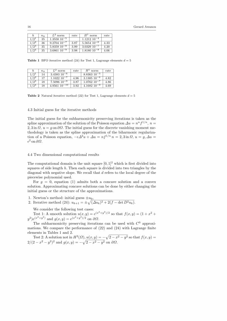
The computational domain is the unit square [0, 1]2 which is first divided intosquares of side length h. Then each square is divided into two triangles by thediagonal with negative slope. We recall that d refers to the local degree of thepiecewise polynomial used.

For g = 0, equation (1) admits both a concave solution and a convexsolution. Approximating concave solutions can be done by either changing theinitial guess or the structure of the approximations.

1. Newton’s method: initial guess ±u0,2. Iterative method (24): uk+1 = ±

√(∆uk)2 + 2(f − detD2uk).

We consider the following test cases:Test 1: A smooth solution u(x, y) = e(x

2+y2)/2 so that f(x, y) = (1 + x2 +

y2)e(x2+y2) and g(x, y) = e(x

2+y2)/2 on ∂Ω.The subharmonicity preserving iterations can be used with C0 approxi-

mations. We compare the performance of (22) and (24) with Lagrange finiteelements in Tables 1 and 2.

Test 2: A solution not inH2(Ω), u(x, y) = −√

2− x2 − y2 so that f(x, y) =

2/(2− x2 − y2)2 and g(x, y) = −√

2− x2 − y2 on ∂Ω.

Methods for Monge-Ampere equation 17

h L2 norm H1 norm1/21 7.6680 10−3 7.4491 10−2

1/22 1.4536 10−3 3.9244 10−2

1/23 9.8727 10−3 2.5112 10−1

1/24 5.6819 10−3 2.4927 10−1

1/25 1.9830 10+4 1.1812 10+6

h L2 norm H1 norm1/21 7.8254 10−3 9.3184 10−2

1/22 1.0646 10−2 9.5201 10−2

1/23 1.1306 10−2 9.6154 10−2

1/24 1.1500 10−2 9.1336 10−2

1/25 1.1625 10−2 8.7785 10−2

1/26 1.1681 10−2 8.5632 10−2

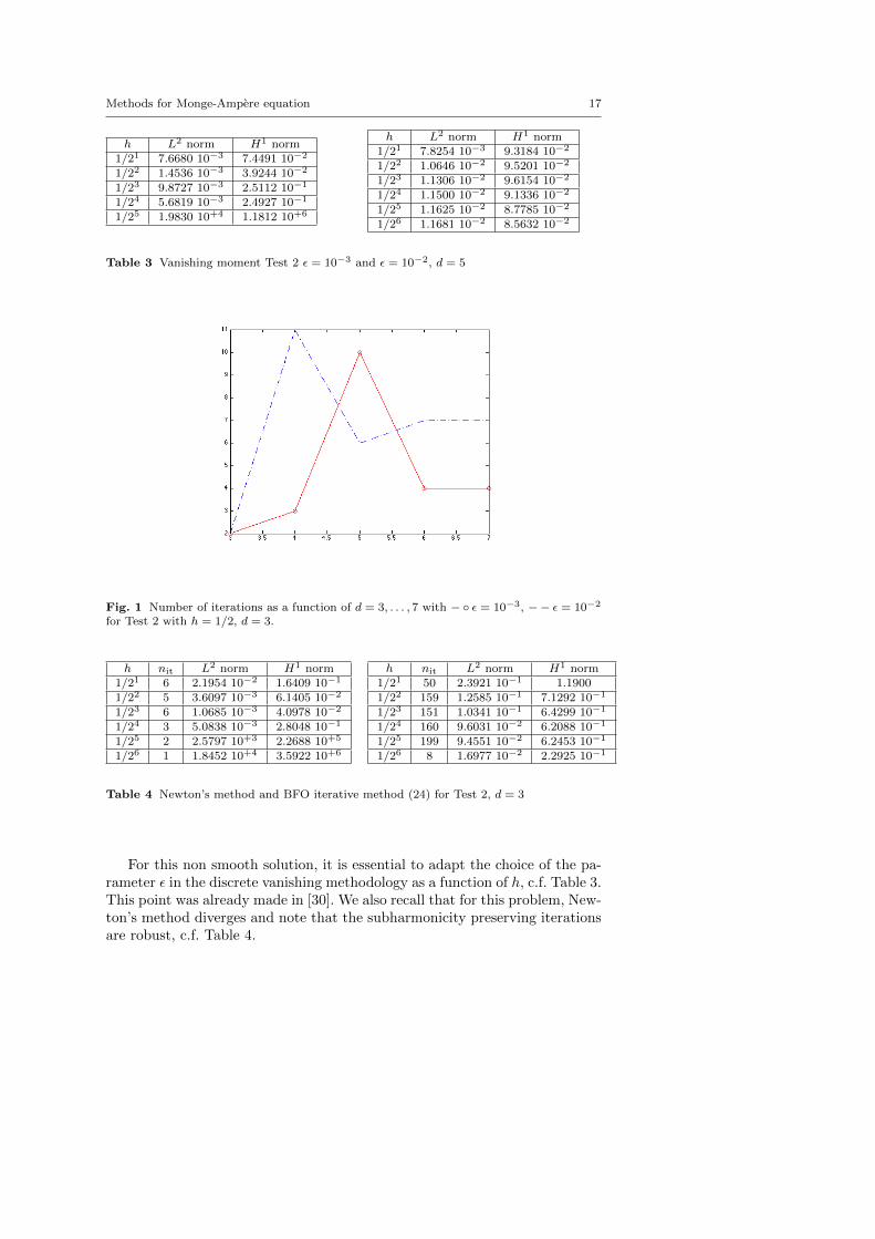
Table 3 Vanishing moment Test 2 ε = 10−3 and ε = 10−2, d = 5

Fig. 1 Number of iterations as a function of d = 3, . . . , 7 with − ε = 10−3, −− ε = 10−2

for Test 2 with h = 1/2, d = 3.

h nit L2 norm H1 norm1/21 6 2.1954 10−2 1.6409 10−1

1/22 5 3.6097 10−3 6.1405 10−2

1/23 6 1.0685 10−3 4.0978 10−2

1/24 3 5.0838 10−3 2.8048 10−1

1/25 2 2.5797 10+3 2.2688 10+5

1/26 1 1.8452 10+4 3.5922 10+6

h nit L2 norm H1 norm1/21 50 2.3921 10−1 1.19001/22 159 1.2585 10−1 7.1292 10−1

1/23 151 1.0341 10−1 6.4299 10−1

1/24 160 9.6031 10−2 6.2088 10−1

1/25 199 9.4551 10−2 6.2453 10−1

1/26 8 1.6977 10−2 2.2925 10−1

Table 4 Newton’s method and BFO iterative method (24) for Test 2, d = 3

For this non smooth solution, it is essential to adapt the choice of the pa-rameter ε in the discrete vanishing methodology as a function of h, c.f. Table 3.This point was already made in [30]. We also recall that for this problem, New-ton’s method diverges and note that the subharmonicity preserving iterationsare robust, c.f. Table 4.

18 Gerard Awanou

d nit L2 norm H1 norm H2 norm3 1 1.2338 10−2 7.6984 10−2 4.4411 10−1

4 3 1.6289 10−3 1.4719 10−2 1.3983 10−1

5 4 1.5333 10−3 8.7312 10−3 6.0412 10−2

6 5 1.2324 10−4 9.7171 10−4 1.0584 10−2

Rate 0.18 0.25d−1 4.58 0.25d 59.96 0.3d+1

Table 5 Newton’s method Test 3, Domain 1 on T1, h = 1

d nit L2 norm H1 norm H2 norm3 1 3.1739 10−3 2.3005 10−2 2.4496 10−1

4 7 3.2786 10−4 3.5626 10−3 5.2079 10−2

5 5 2.4027 10−5 3.9210 10−4 8.8868 10−3

6 6 1.3821 10−6 2.2369 10−5 6.0918 10−4

Rate 0.65 0.075d−1 28.96 0.1d 849.85 0.14d+1

Table 6 Newton’s method Test 3, Domain 1 on T2, h = 1/2

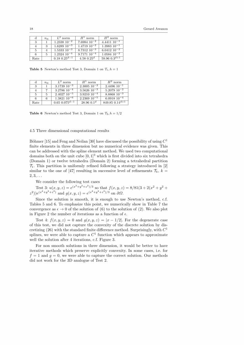
4.5 Three dimensional computational results

Bohmer [15] and Feng and Neilan [30] have discussed the possibility of using C1

finite elements in three dimension but no numerical evidence was given. Thiscan be addressed with the spline element method. We used two computationaldomains both on the unit cube [0, 1]3 which is first divided into six tetrahedra(Domain 1) or twelve tetrahedra (Domain 2) forming a tetrahedral partitionT1. This partition is uniformly refined following a strategy introduced in [2]similar to the one of [47] resulting in successive level of refinements Tk, k =2, 3, . . .

We consider the following test cases

Test 3: u(x, y, z) = e(x2+y2+z2)/3 so that f(x, y, z) = 8/81(3 + 2(x2 + y2 +

z2))e(x2+y2+z2) and g(x, y, z) = e(x

2+y2+z2)/3 on ∂Ω.

Since the solution is smooth, it is enough to use Newton’s method, c.f.Tables 5 and 6. To emphasize this point, we numerically show in Table 7 theconvergence as ε→ 0 of the solution of (6) to the solution of (2). We also plotin Figure 2 the number of iterations as a function of ε.

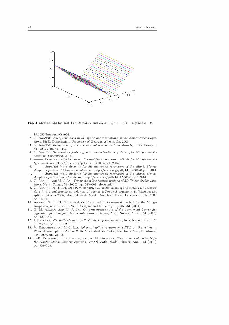
Test 4: f(x, y, z) = 0 and g(x, y, z) = |x − 1/2|. For the degenerate caseof this test, we did not capture the convexity of the discrete solution by dis-cretizing (26) with the standard finite difference method. Surprisingly, with C1

splines, we were able to capture a C1 function which appears to approximatewell the solution after 4 iterations, c.f. Figure 3.

For non smooth solutions in three dimension, it would be better to haveiterative methods which preserve explicitly convexity. In some cases, i.e. forf = 1 and g = 0, we were able to capture the correct solution. Our methodsdid not work for the 3D analogue of Test 2.

Methods for Monge-Ampere equation 19

ε L2 norm H1 norm H2 norm10−1 6.6870 10−2 3.9292 10−1 2.885210−2 1.8832 10−2 1.3137 10−1 1.588210−3 2.4237 10−3 2.5273 10−2 5.3206 10−1

10−4 2.5661 10−4 3.2633 10−3 7.9936 10−2

10−5 3.1058 10−5 5.0367 10−4 1.2543 10−2

10−6 2.3519 10−5 3.9165 10−4 8.9744 10−3

10−7 2.3964 10−5 3.9193 10−4 8.8921 10−3

10−10 2.4027 10−5 3.9210 10−4 8.8868 10−3

0 2.4027 10−5 3.9210 10−4 8.8868 10−3

Table 7 3D numerical robustness Test 3, Domain 1 on T2, h = 1/2, d = 5

Fig. 2 Number of iterations as a function of j = 1, . . . , 10 with ε = 10−j for Test 3 withh = 1/2, d = 5 on Domain 1.

Acknowledgements

The author would like to thank the referees for a careful reading of the paperand their suggestions which lead to a better paper. This work began when theauthor was supported in part by a 2009-2013 Sloan Foundation Fellowship andcontinued while the author was in residence at the Mathematical Sciences Re-search Institute (MSRI) in Berkeley, California, Fall 2013. The MSRI receivesmajor funding from the National Science Foundation under Grant No. 0932078000. The author was partially supported by NSF DMS grant No 1319640.

References

1. G. Awanou, Standard finite elements for the numerical resolution of the ellip-tic Monge-Ampere equation: classical solutions. IMA J Numer Anal (2014) doi:

20 Gerard Awanou

Fig. 3 Method (26) for Test 4 on Domain 2 and I3, h = 1/8, d = 5, r = 1, plane z = 0.

10.1093/imanum/dru028.2. G. Awanou, Energy methods in 3D spline approximations of the Navier-Stokes equa-

tions, Ph.D. Dissertation, University of Georgia, Athens, Ga, 2003.3. G. Awanou, Robustness of a spline element method with constraints, J. Sci. Comput.,

36 (2008), pp. 421–432.4. G. Awanou, On standard finite difference discretizations of the elliptic Monge-Ampere

equation. Submitted, 2014.5. , Pseudo transient continuation and time marching methods for Monge-Ampere

type equations. http://arxiv.org/pdf/1301.5891v4.pdf, 2014.6. , Standard finite elements for the numerical resolution of the elliptic Monge-

Ampere equation: Aleksandrov solutions. http://arxiv.org/pdf/1310.4568v3.pdf, 2014.7. , Standard finite elements for the numerical resolution of the elliptic Monge-

Ampere equation: mixed methods. http://arxiv.org/pdf/1406.5666v1.pdf, 2014.8. G. Awanou and M.-J. Lai, Trivariate spline approximations of 3D Navier-Stokes equa-

tions, Math. Comp., 74 (2005), pp. 585–601 (electronic).9. G. Awanou, M.-J. Lai, and P. Wenston, The multivariate spline method for scattered

data fitting and numerical solution of partial differential equations, in Wavelets andsplines: Athens 2005, Mod. Methods Math., Nashboro Press, Brentwood, TN, 2006,pp. 24–74.

10. Awanou, G., Li, H.: Error analysis of a mixed finite element method for the Monge-Ampere equation. Int. J. Num. Analysis and Modeling 11, 745–761 (2014)

11. G. M. Awanou and M. J. Lai, On convergence rate of the augmented Lagrangianalgorithm for nonsymmetric saddle point problems, Appl. Numer. Math., 54 (2005),pp. 122–134.

12. I. Babuska, The finite element method with Lagrangian multipliers, Numer. Math., 20(1972/73), pp. 179–192.

13. V. Baramidze and M.-J. Lai, Spherical spline solution to a PDE on the sphere, inWavelets and splines: Athens 2005, Mod. Methods Math., Nashboro Press, Brentwood,TN, 2006, pp. 75–92.

14. J.-D. Benamou, B. D. Froese, and A. M. Oberman, Two numerical methods forthe elliptic Monge-Ampere equation, M2AN Math. Model. Numer. Anal., 44 (2010),pp. 737–758.

Methods for Monge-Ampere equation 21

15. K. Bohmer, On finite element methods for fully nonlinear elliptic equations of secondorder, SIAM J. Numer. Anal., 46 (2008), pp. 1212–1249.

16. K. Bohmer, Numerical methods for nonlinear elliptic differential equations: a synopsis,Oxford University Press, USA, 2010.

17. M. Bouchiba and F. B. Belgacem, Numerical solution of Monge-Ampere equation,Math. Balkanica (N.S.), 20 (2006), pp. 369–378.

18. S. C. Brenner, T. Gudi, M. Neilan, and L.-Y. Sung, C0 penalty methods for thefully nonlinear Monge-Ampere equation, Math. Comp., 80 (2011), pp. 1979–1995.

19. S. C. Brenner and M. Neilan, Finite element approximations of the three dimensionalMonge-Ampere equation, ESAIM Math. Model. Numer. Anal., 46 (2012), pp. 979–1001.

20. S. C. Brenner and L. R. Scott, The mathematical theory of finite element methods,vol. 15 of Texts in Applied Mathematics, Springer-Verlag, New York, second ed., 2002.

21. W. Dahmen, Convexity and Bernstein-Bezier polynomials, in Curves and surfaces(Chamonix-Mont-Blanc, 1990), Academic Press, Boston, MA, 1991, pp. 107–134.

22. Davydov, O., Saeed, A.: Numerical solution of fully nonlinear elliptic equations byBohmer’s method. J. Comput. Appl. Math. 254, 43–54 (2013)

23. E. J. Dean and R. Glowinski, Numerical solution of the two-dimensional ellipticMonge-Ampere equation with Dirichlet boundary conditions: an augmented Lagrangianapproach, C. R. Math. Acad. Sci. Paris, 336 (2003), pp. 779–784.

24. , Numerical solution of the two-dimensional elliptic Monge-Ampere equation withDirichlet boundary conditions: a least-squares approach, C. R. Math. Acad. Sci. Paris,339 (2004), pp. 887–892.

25. E. J. Dean and R. Glowinski, Numerical methods for fully nonlinear elliptic equationsof the Monge-Ampere type, Comput. Methods Appl. Mech. Engrg., 195 (2006), pp. 1344–1386.

26. Feng, X., Neilan, M.: Convergence of a fourth-order singular perturbation of the n-dimensional radially symmetric Monge–Ampere equation. Appl. Anal. 93(8), 1626–1646(2014)

27. X. Feng and M. Neilan, Error analysis for mixed finite element approximations ofthe fully nonlinear Monge-Ampere equation based on the vanishing moment method,SIAM J. Numer. Anal., 47 (2009), pp. 1226–1250.

28. X. Feng and M. Neilan, A modified characteristic finite element method for a fullynonlinear formulation of the semigeostrophic flow equations, SIAM J. Numer. Anal.,47 (2009), pp. 2952–2981.

29. X. Feng and M. Neilan, Vanishing moment method and moment solutions for secondorder fully nonlinear partial differential equations, J. Sci. Comput., 38 (2009), pp. 74–98.

30. X. Feng and M. Neilan, Analysis of Galerkin methods for the fully nonlinear Monge-Ampere equation, J. Sci. Comput., 47 (2011), pp. 303–327.

31. B. Froese and A. Oberman, Convergent finite difference solvers for viscosity solutionsof the elliptic Monge-Ampere equation in dimensions two and higher, SIAM J. Numer.Anal., 49 (2011), pp. 1692–1714.

32. B. D. Froese and A. M. Oberman, Fast finite difference solvers for singular solutionsof the elliptic Monge-Ampere equation, J. Comput. Phys., 230 (2011), pp. 818–834.

33. B. D. Froese and A. M. Oberman, Convergent filtered schemes for the Monge-Amperepartial differential equation, SIAM J. Numer. Anal., 51 (2013), pp. 423–444.

34. R. Glowinski, Numerical methods for fully nonlinear elliptic equations, in ICIAM 07—6th International Congress on Industrial and Applied Mathematics, Eur. Math. Soc.,Zurich, 2009, pp. 155–192.

35. C. E. Gutierrez, The Monge-Ampere equation, Progress in Nonlinear DifferentialEquations and their Applications, 44, Birkhauser Boston Inc., Boston, MA, 2001.

36. G. Harris and C. Martin, The roots of a polynomial vary continuously as a functionof the coefficients, Proc. Amer. Math. Soc., 100 (1987), pp. 390–392.

37. X.-L. Hu, D.-F. Han, and M.-J. Lai, Bivariate splines of various degrees for numericalsolution of partial differential equations, SIAM J. Sci. Comput., 29 (2007), pp. 1338–1354 (electronic).

38. M.-J. Lai and L. L. Schumaker, Spline functions on triangulations, vol. 110 of Ency-clopedia of Mathematics and its Applications, Cambridge University Press, Cambridge,2007.

22 Gerard Awanou

39. O. Lakkis and T. Pryer, A finite element method for nonlinear elliptic problems,SIAM J. Sci. Comput., 35 (2013), pp. A2025–A2045.

40. B. Mohammadi, Optimal transport, shape optimization and global minimization, C. R.Math. Acad. Sci. Paris, 344 (2007), pp. 591–596.

41. M. Neilan, A nonconforming Morley finite element method for the fully nonlinearMonge-Ampere equation, Numer. Math., 115 (2010), pp. 371–394.

42. Neilan, M.: Finite element methods for fully nonlinear second order PDEs based on adiscrete Hessian with applications to the Monge–Ampere equation. J. Comput. Appl.Math. 263, 351–369 (2014)

43. M. Neilan, Quadratic finite element approximations of the Monge-Ampere equation,J. Sci. Comput., 54 (2013), pp. 200–226.

44. T. K. Nilssen, X.-C. Tai, and R. Winther, A robust nonconforming H2-element,Math. Comp., 70 (2001), pp. 489–505.

45. A. M. Oberman, Wide stencil finite difference schemes for the elliptic Monge-Ampereequation and functions of the eigenvalues of the Hessian, Discrete Contin. Dyn. Syst.Ser. B, 10 (2008), pp. 221–238.

46. V. I. Oliker and L. D. Prussner, On the numerical solution of the equation(∂2z/∂x2)(∂2z/∂y2) − ((∂2z/∂x∂y))2 = f and its discretizations. I, Numer. Math.,54 (1988), pp. 271–293.

47. M. E. G. Ong, Uniform refinement of a tetrahedron, SIAM J. Sci. Comput., 15 (1994),pp. 1134–1144.

48. A. M. Ostrowski, Solution of equations and systems of equations, Pure and AppliedMathematics, Vol. IX. Academic Press, New York-London, 1960.

49. J. Rauch and B. A. Taylor, The Dirichlet problem for the multidimensional Monge-Ampere equation, Rocky Mountain J. Math., 7 (1977), pp. 345–364.

50. A.-V. Vuong, C. Heinrich, and B. Simeon, ISOGAT: a 2D tutorial MATLAB codefor isogeometric analysis, Comput. Aided Geom. Design, 27 (2010), pp. 644–655.

51. V. Zheligovsky, O. Podvigina, and U. Frisch, The Monge-Ampere equation: variousforms and numerical solution, J. Comput. Phys., 229 (2010), pp. 5043–5061.