Embed Size (px)
Citation preview

AFFINE MANIFOLDS, SYZ GEOMETRY AND THE“Y” VERTEX
JOHN LOFTIN, SHING-TUNG YAU, AND ERIC ZASLOW
Abstract. We study the real Monge-Ampere equation in two andthree dimensions, both from the point of view of the SYZ conjec-ture, where solutions give rise to semi-flat Calabi-Yau’s and inaffine differential geometry, where solutions yield parabolic affinesphere hypersurfaces. We find explicit examples, connect the holo-morphic function representation to Hitchin’s description of specialLagrangian moduli space, and construct the developing map ex-plicitly for a singularity corresponding to the type In elliptic fiber(after hyper-Kahler rotation). Following Baues and Cortes, weshow that various types of metric cones over two-dimensional ellip-tic affine spheres generate solutions of the Monge-Ampere equationin three dimensions. We then prove a local and global existencetheorem for an elliptic affine two-sphere metric with prescribedsingularities. The metric cone over the two-sphere minus threepoints yields a parabolic affine sphere with singularities along a“Y”-shaped locus. This gives a semi-flat Calabi-Yau metric in aneighborhood of the “Y” vertex.
1. Introduction
The basic question we would like to understand is, What does the ge-ometry of a Calabi-Yau manifold look like near (or “at”) the large com-plex structure limit point? In order to answer this question, one firstfixes the ambiguity of rescaling the metric by an overall constant. Gro-mov proved that Ricci-flat manifolds with fixed diameter have a limitunder the Gromov-Hausdorff metric (on the space of metric spaces).
Now by the conjecture of [25], one expects that near the limit, theCalabi-Yau has a fibration by special Lagrangian submanifolds whichare getting smaller and smaller (than the base). The reason can befound by looking at the mirror large radius limit. Fibers are mirror tothe zero brane, and the base is mirror to the 2n brane, which becomeslarge at large radius. Metrically, the Calabi-Yau geometry should beroughly a fibration over the moduli space of special Lagrangian tori (T ).The dual fibration is by dual tori, Hom (π1(T ),R)/Hom (π1(T ),Z).The flat fiber geometry of the dual torus fibration has a flat fiber dual,
1
AFFINE MANIFOLDS, SYZ GEOMETRY AND THE “Y” VERTEX 2
which is not the same as the original geometry, but should be the sameafter corrections by disk instantons. These should get small in the limitof small tori, though. Namely, we expect that the Gromov-Hausdorfflimit of a fixed-diameter Calabi-Yau manifold approaching a maximal-degeneration point carries the same geometry as the moduli space ofspecial Lagrangian tori. That is, it is a manifold (and an affine manifoldat that) of half the dimension.
Further, the Calabi-Yau near the limit should be “asymptoticallyclose” to the standard flat torus fibration over special Lagrangian torimoduli space, whose fibers are the flat tori (we get this from dual torusconsiderations applied to the mirror manifold). This space is a quotientof the tangent space of the moduli space (which is Hessian), and theCalabi-Yau condition means that the limiting affine manifold metricshould be Monge-Ampere (det (Hess Φ) = 1). Global considerationsrequire that the lattice defining the torus (generated by the vectorsassociated to the Hessian coordinates) is well-defined, meaning thatthe Monge-Ampere manifold has affine transition functions in the semi-direct product of SL(n,Z) with Rn translations.
The above is an informal (read: “physical”) explanation behind theconjecture made independently by Gross-Wilson [13] and Kontsevich-Soibelman [16] (it appears in the work of Fukaya [9] as well), and provedby Gross-Wilson for the special case of K3 surfaces [13]. Their proofuses the Ooguri-Vafa [21] metric in the neighborhood of a torus degen-eration to build an approximate Ricci-flat metric on the entirety of anelliptic K3 with 24 singular fibers (with an elliptic-fibration/stringy-cosmic-string metric outside the patches describing degenerations).
Another aspect of the conjecture is that the limiting manifold hassingularities in codimension two, with monodromy transformations de-fined for each loop about the singular set. Gross has shown the exis-tence of a limiting singular set of codimension two for (non-Lagrangian)torus fibrations on toric three-fold Calabi-Yau’s, and further has shownthat the limiting singular set has the structure of a trivalent graph.Taking our cue from this work, then in three dimensions a point onthe limiting manifold may be a smooth point, a point near an intervalsingularity, or the trivalent vertex of a “Y”-shaped singularity locus(these vertices have a subclassification based on the monodromies nearthe vertex). Examples of explicit Monge-Ampere metrics for points ofthe first two types are known, the interval singularity reducing to thean interval times the two-fold point singularity. The absence of a localmetric model of a trivalent vertex singularity limits our ability to provethis conjecture in three dimensions. Even if we had such a model, itmight not suffice to prove the conjectures about the limiting metric,
AFFINE MANIFOLDS, SYZ GEOMETRY AND THE “Y” VERTEX 3
just as the non-Ooguri-Vafa elliptic fibration metric does not sufficeeven in the two-dimensional case. Still, we regard the existence of asemi-flat Calabi-Yau metric near the “Y” vertex as an important firststep in addressing these conjectures in three dimensions.1
We therefore concern ourselves with studying Monge-Ampere man-ifolds in low dimensions, with the goal of finding a local model for atrivalent degeneration of special Lagrangian tori. Taking our modelto be a metric cone over a thrice-punctured two-sphere, we have, byan argument of Baues and Cortes, that the sphere metric should bean elliptic affine sphere on S2 with three singularities. The singularitytype of the metric at the three points is fixed by the pole behaviorof a holomorphic cubic form. Our main result is a proof of the exis-tence of such an elliptic affine sphere, hence its cone, which solves theMonge-Ampere equation with the desired singular locus.
The plan of attack is as follows. We study the Monge-Ampere equa-tion and Hessian manifolds in Section 2, exhibiting a few new solutionsin three-dimensions. In Section 3, we study the relation between el-liptic fibrations (“stringy cosmic string”) and Hessian coordinates intwo dimensions. In Section 4, we construct two-dimensional Monge-Ampere solutions as parabolic affine two-spheres in R3, using affinedifferential geometry techniques developed by Simon and Wang. Wefind the affine coordinates and calculate the monodromy for some ofour solutions in Section 5. In Section 6 we discuss parabolic affinespheres which occur as radial (“cone”) metrics, generalizing Baues andCortes’s result to some new examples. Simon and Wang’s techniquesalso give equations for singular elliptic affine spheres, the cone overwhich yields three-dimensional Monge-Ampere solutions. In Section 7we employ this technique and study the local structure near a singu-larity of the elliptic affine sphere. Using this local analysis, we turn toglobal case and complete the existence proof. The Calabi-Yau metricnear the “Y” vertex is then constructed as a cone.
2. Hessian Metrics and the Monge-Ampere Equation
We recall that a metric is of Hessian type if in coordinates xi ithas the form ds2 = Φijdx
i ⊗ dxj, where Φij = ∂2Φ/∂xi∂xj. Hitchinproved [14] that natural metric (“McLean” or “Weil-Petersson”) onmoduli space of special Lagrangian submanifolds naturally has this
1This vertex is not the same as the topological vertex of [1], which appears at acorner of the toric polyhedron describing the Calabi-Yau. The relation between thetoric description of the Calabi-Yau and the singularities of the special Lagrangiantorus fibration has been discussed in [12].
AFFINE MANIFOLDS, SYZ GEOMETRY AND THE “Y” VERTEX 4
structure, and the semi-flat metric on the complexification (by flatbundles) defined by the Kahler potential Φ is Ricci flat if
(1) det (Φij) = 1.
In Hessian coordinates we can compute the Christoffel symbols Γijk =12ΦilΦjkl (where ∇j∂k = Γijk∂i), and defining the curvature tensor
Rijkl = ∂iΓ
kjl + ΓkimΓmjl − (i↔ j) by [∇i,∇j]∂k = Rij
kl∂l, we find
(2) Rijkl = −1
4Φab[ΦikaΦjlb − ΦjkaΦilb].
2.1. Hessian Coordinate Transformations. One asks, what coor-dinate transformations preserve the Hessian form of the metric? Ifwe try to write ds2 = Φijdx
idxj = Ψabdyadyb = Ψaby
aiybjdx
idxj,then the consistency equations Φijk = Φkji yield conditions on thecoordinate transformation y(x). Specifically, we have ∂k(Ψaby
aiybj) =
∂i(Ψabyaky
bj), which is equivalent to
Ψab(yaiybjk − yakybij) = 0.
In two dimensions, for example, there can be many solutions to theseequations. In Euclidean space Ψab = δab with coordinates ya, if weput y1 = f(x1 + x2) + g(x1 − x2) and y2 = f(x1 + x2) − g(x1 − x2),then the equations are solved and we can find Φ(x). For example, iff(s) = g(s) = s2/2, we find Φ(x) = [(x1)4 + 6x1x2 + (x2)4]/12.
Note that this transformation is not affine. Thus Hessian metricsmay exist on non-affine manifolds. Hessian manifolds can be charac-terized as locally having an abelian Lie algebra of gradient vector fieldsacting simply transitively [23]. Though Hessian manifolds are moregeneral than affine manifolds, a Hessian manifold appearing as a mod-uli space of special Lagrangian tori must have an affine structure. Wetherefore focus on affine Hessian manifolds in this paper.
2.2. Examples of Monge-Ampere Metrics. As we will see in Sec-tion 3, there are many Monge-Ampere metrics in two dimensions, buta paucity of examples in three or more dimensions. Here we provide afew solutions.
Example 1. In dimension d consider the ansatz Φ = Φ(r), wherer =
√∑i(x
i)2. As shown by Calabi, the equation (1) is solved if
(3) Φ(r) =
∫(1 + rd)1/d.
The rescalings r → cr and Φ→ cΦ also have constant det(Hess Φ). Forexample, in two dimensions (d = 2), Φ(r) = sinh−1(r) + r
√1 + r2 is a
solution.

AFFINE MANIFOLDS, SYZ GEOMETRY AND THE “Y” VERTEX 5
Example 2. We now take d = 3 and make the axial ansatz Φ =Φ(ρ, z), where ρ =
√x2 + y2. One computes det(Hess Φ) = Φρ
ρ[ΦzzΦρρ−
(Φρz)2]. We search for a solution of the form Φ(ρ, z) = A(ρ)B(z), which
leads to the equation
AA′A′′B2B′′ − (A′)3B(B′)2 = ρ.
We take A = 34ρ4/3, so (A′)3 = ρ and AA′A′′ = ρ/4. This gives the
equation B2B′′ − 4B(B′)2 = 4. The substitution B = −21/3v−1/3 leadsto the equation v′′ = 6v2. This equation is satisfied by the Weierstrassp-function corresponding to a Weierstrass elliptic curve with g2 = 0 andg3, a constant of integration, real (so that p is real). The full solutionis then
Φ(ρ, z) = −3 · 2−5/3ρ4/3pτ (z + c)−1/3,
where τ = τ(g2 = 0, g3 < 0) and c is an arbitrary constant. In orderfor this function to define a metric, its Hessian matrix must be positivedefinite. One checks that all diagonal minors are positive as long asp < 0 and g3 < 0 (hence the condition above).
Example 3. In three dimensions, when Φ = Φ(t) for some functiont(x1, x2, x3), there is sometimes simplification of the Monge-Ampereequation – for example, t = r leads to the simple solution (3). ForΦ = Φ(t(x)), we compute:
det(Φij) = (Φ′)3det(tij) +
(Φ′)2(Φ′′)[t21(t22t33 − t223) + t22(t33t11 − t213)+
t23(t11t22 − t212) + 2t1t2(t13t23 − t12t33) +
2t2t3(t12t13 − t11t23) + 2t1t3(t12t23 − t22t13)] .
We reduce to an ODE when det(tij) and the term in brackets can bewritten in terms of t alone.
For example, if t = xyz we find det(tij) = 2t, and the term inbrackets is 3t2. This leads to (Φ′)3(3t2) + (Φ′)2(Φ′′)(2t) = 1, whichis solved by putting y = (Φ′)3. Then (yt2)′ = 1, which leads to Φ =∫
(Ct−2 + t−1)1/3dt. One calculates that Hess(Φ) is positive definite ift < 0 and |C| > |t|.Example 4. For another example of the type in Ex. 3, we put t =xy + yz + zx, then det(tij) = 2 and the term in brackets is 4t. We findΦ =
∫(1/2+Ct−3/2)1/3dt. This solution is also convex in a C-dependent
region.
AFFINE MANIFOLDS, SYZ GEOMETRY AND THE “Y” VERTEX 6
3. Monge-Ampere Metrics and the Stringy Cosmic String
Using a hyper-Kahler rotation we can treat any elliptic surface asa special Lagrangian fibration and try to find its associated Hessiancoordinates and – if the fibers are flat – the corresponding solution tothe Monge-Ampere equation.
In the case of the stringy cosmic string, we begin with a semi-flatfibration with torus fiber coordinates t ∼ t + 1 and x ∼ x + 1. As aholomorphic fibration, the stringy cosmic string is defined by a holo-morphic modulus τ(z). One can derive the Kahler potential through theGibbons-Hawking ansatz (with ∂/∂t as Killing vector) using connectionone-form A = −τ1dx and potential V = τ2 (so ∗dA = dV ), then solvingfor the holomorphic coordinate. One finds ξ = t+τ(z)x = t+τ1x+iτ2x.The hyper-Kahler structure is specified by the forms
ω1 = dx ∧ dt+ (i
2)τ2dz ∧ dz
ω2 + iω3 = dz ∧ dξ.
The stringy cosmic string solution starts directly from the Kahler po-tential K(z, ξ) = ξ2/τ2 + k(z, z), where ∂z∂zk = τ2.
We seek the Hessian coordinates for the base of the semi-flat specialLagranian torus fibration. In coordinates (x, t, z1, z2) the metric hasthe block diagonal form
(4) Q⊕R ≡ 1
τ2
(|τ |2 τ1
τ1 1
)⊕(τ2 00 τ2
).
For a semi-flat fibration over a Hessian manifold in Hessian coordinates,the base-dependent metric on the fiber looks the same as the metric onthe base. Therefore, we would need to find coordinates u1(z, z), u2(z, z)so that the metric in u-space looks like Q in (4). This is accomplishedif the change of basis matrix Mij = ∂zi/∂uj obeys MTM = Q/τ2. A
calculation reveals the general solution to be M = OM, where M =
1τ2
(τ2 τ1
0 1
), and O is an orthogonal matrix. The same result can be
obtained using Hitchin’s method, which we now review.Hitchin [14] obtains Hessian coordinates on the moduli space of spe-
cial Lagrangian submanifolds from period integrals. In order to applythis technique here we first make a hyper-Kahler rotation, so that thefibration is special Lagrangian, by putting ω = ω2, ImΩ = ω3. Ex-plicitly, for each base coordinate zi we construct closed one forms onthe Lagrangian L, defined by ι∂/∂ziω = θi and compute the periodsλij =
∫Aiθj, where Ai is a basis for H1(L,Z). In our case we readily
AFFINE MANIFOLDS, SYZ GEOMETRY AND THE “Y” VERTEX 7
find θ1 = dt+ τ1dx, θ2 = −τ2dx, and, using the basis A1 = t→ t+ 1,A2 = −x→ x+ 1, we get
λij =
(1 0−τ1 τ2
).
The forms λijdzj are closed on the base and we set them equal to dui.This defines the coordinates dui up to constants, and we find u1 = z1,u2 = −Reφ, where ∂zφ = τ. To connect with the solution above, one
easily inverts the matrix λij = ∂ui/∂zj to find the matrix ∂zi/∂uj = M.
Remark. The change of coordinates u2 ↔ −u2 preserves the Monge-Ampere equation, and we sometimes use the latter in what follows.
Legendre dual coordinates vi are defined as follows. Define (d− 1)-forms ψi (here d = 2 so the ψ’s are also one-forms) by putting Ω =dzi ∧ ψi and compute the periods µij =
∫Biψj, where Bj ∈ Hd−1(L,Z)
are Poincare dual to the Ai. In our example, ψ1 = τ2dx, ψ2 = dt+τ1dx,B1 = x→ x+ 1, B2 = t→ t+ 1, and
µij =
(τ2 τ1
0 1
).
(Note λTµ is symmetric, as required.) Setting dvi = µijdzj we findv1 = Imφ and v2 = z2.
Hitchin showed that the coordinates ui and vi are related by theLegendre transformation defined by the function Φ whose Hessian givesthe metric. Namely, vi = ∂Φ/∂ui. We can think of Φ as a function ofthe zi(uj) and differentiate with respect to uj using the chain rule. (Wefind ∂zi/∂uj by inverting the matrix of derivatives ∂ui/∂zj.) One finds
Φz1 = Im φ− τ1z2, Φz2 = τ2z2.
(For the transformed potential Ψ we have Ψz1 = τ2z1 and Ψz2 =τ1z1−Reφ.) The solution can be given in terms of another holomorphicantiderivative,2 χ, such that ∂zχ = φ.
Φ = −z2Reφ + Imχ.
Note, then, that being able to write down the explicit Hessian potentialdepends only on our ability to integrate τ and invert the functionsui(zj). The Legendre-transformed potential is Ψ = z1Imφ− Imχ.
2V. Cortes has found a generalization of this potential as the defining function ofparabolic affine hyperspheres – equivalently, Hessian manifolds obeying the Monge-Ampere equation – described by holomorphic data. The example above is thesimplest instance of his more general approach, and is due to Blaschke.
AFFINE MANIFOLDS, SYZ GEOMETRY AND THE “Y” VERTEX 8
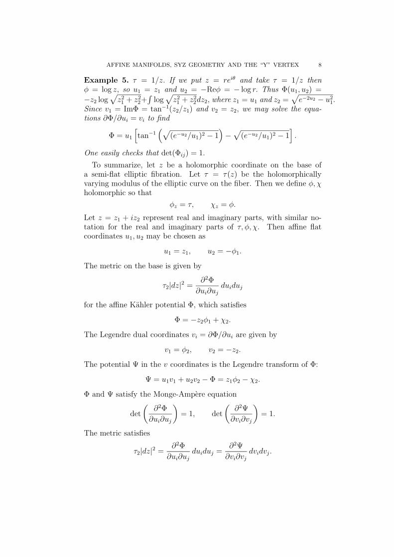
Example 5. τ = 1/z. If we put z = reiθ and take τ = 1/z thenφ = log z, so u1 = z1 and u2 = −Reφ = − log r. Thus Φ(u1, u2) =
−z2 log√z2
1 + z22+∫
log√z2
1 + z22dz2, where z1 = u1 and z2 =
√e−2u2 − u2
1.Since v1 = ImΦ = tan−1(z2/z1) and v2 = z2, we may solve the equa-tions ∂Φ/∂ui = vi to find
Φ = u1
[tan−1
(√(e−u2/u1)2 − 1
)−√
(e−u2/u1)2 − 1].
One easily checks that det(Φij) = 1.
To summarize, let z be a holomorphic coordinate on the base ofa semi-flat elliptic fibration. Let τ = τ(z) be the holomorphicallyvarying modulus of the elliptic curve on the fiber. Then we define φ, χholomorphic so that
φz = τ, χz = φ.
Let z = z1 + iz2 represent real and imaginary parts, with similar no-tation for the real and imaginary parts of τ, φ, χ. Then affine flatcoordinates u1, u2 may be chosen as
u1 = z1, u2 = −φ1.
The metric on the base is given by
τ2|dz|2 =∂2Φ
∂ui∂ujduiduj
for the affine Kahler potential Φ, which satisfies
Φ = −z2φ1 + χ2.
The Legendre dual coordinates vi = ∂Φ/∂ui are given by
v1 = φ2, v2 = −z2.
The potential Ψ in the v coordinates is the Legendre transform of Φ:
Ψ = u1v1 + u2v2 − Φ = z1φ2 − χ2.
Φ and Ψ satisfy the Monge-Ampere equation
det
(∂2Φ
∂ui∂uj
)= 1, det
(∂2Ψ
∂vi∂vj
)= 1.
The metric satisfies
τ2|dz|2 =∂2Φ
∂ui∂ujduiduj =
∂2Ψ
∂vi∂vjdvidvj.
AFFINE MANIFOLDS, SYZ GEOMETRY AND THE “Y” VERTEX 9
4. Explicit Solutions for the Developing Map
This is a model of a 2-dimensional parabolic affine sphere. At firstwe work from the structure equations, to find an ODE problem tosolve. We find a family of solutions indexed by an integer k. The k = 0case has monodromy, and is found to be equivalent to the holomorphicrepresentation seen earlier. with τ = 2i log z. The ODE approach ismore difficult, but is probably all that’s available in the elliptic affinesphere case. Moreover, the ODE approach has been used successfullyto calculate monodromy for hyperbolic affine spheres [19], and also for aglobal existence result for parabolic affine spheres on S2 minus singularpoints [20]. (Recall we are interested in elliptic affine spheres since acone over an elliptic affine sphere in dimension two is a parabolic affinesphere in dimension three.)
4.1. Simon and Wang’s developing map. U. Simon and C.P. Wang[24] formulate the condition for a two-dimensional surface to be anaffine sphere in terms of the conformal geometry given by the affinemetric. Since we rely heavily on this work, we give a version of thearguments here for the reader’s convenience. For basic background onaffine differential geometry, see Calabi [6], Cheng-Yau [7] and Nomizu-Sasaki [22].
Consider a 2-dimensional parabolic affine sphere in R3. Then theaffine metric gives a conformal structure, and we choose a local confor-mal coordinate z = x+ iy on the hypersurface. Then the affine metricis given by h = eψ|dz|2 for some function ψ. Parametrize the surface
by f : D → R3, with D a domain in C. Since e− 1
2ψfx, e
− 12ψfy is
an orthonormal basis for the tangent space, the affine normal ξ mustsatisfy this volume condition (see e.g. [22])
(5) det(e−12ψfx, e
− 12ψfy, ξ) = 1,
which implies
(6) det(fz, fz, ξ) = 12ieψ.
Now only consider parabolic affine spheres. In this case, the affinenormal ξ is a constant vector, and we have
(7)
DXY = ∇XY + h(X,Y )ξ
DXξ = 0
Here D is the canonical flat connection on R3, ∇ is a flat connection,and h is the affine metric.
It is convenient to work with complexified tangent vectors, and weextend ∇, h and D by complex linearity. Consider the frame for the
AFFINE MANIFOLDS, SYZ GEOMETRY AND THE “Y” VERTEX 10
tangent bundle to the surface e1 = fz = f∗(∂∂z
), e1 = fz = f∗(∂∂z
).Then we have
(8) h(fz, fz) = h(fz, fz) = 0, h(fz, fz) = 12eψ.
Consider θ the matrix of connection one-forms
∇ei = θji ej, i, j ∈ 1, 1,
and θ the matrix of connection one-forms for the Levi-Civita connec-tion. By (8)
(9) θ11 = θ1
1 = 0, θ11 = ∂ψ, θ1
1 = ∂ψ.
The difference θ − θ is given by the Pick form. We have
θji − θji = Cj
ikρk,
where ρ1 = dz, ρ1 = dz is the dual frame of one-forms. Now wedifferentiate (6) and use the structure equations (7) to conclude
θ11 + θ1
1 = dψ.
This implies, together with (9), the apolarity condition
C11k + C 1
1k = 0, k ∈ 1, 1.
Then, when we lower the indices, the expression for the metric (8)implies that
C11k + C11k = 0.
Now Cijk is totally symmetric on three indices [7, 22]. Therefore, theprevious equation implies that all the components of C must vanishexcept C111 and C111 = C111.
This discussion completely determines θ:
(10)
(θ1
1 θ11
θ11 θ1
1
)=
(∂ψ C1
11dz
C 111dz ∂ψ
)=
(∂ψ Ue−ψdz
Ue−ψdz ∂ψ
),
where we define U = C 111e
ψ.Recall that D is the canonical flat connection induced from R
3.(Thus, for example, Dfzfz = D ∂
∂zfz = fzz.) Using this statement,
together with (8) and (10), the structure equations (7) become
(11)
fzz = ψzfz + Ue−ψfzfzz = Ue−ψfz + ψzfz
fzz = 12eψξ
AFFINE MANIFOLDS, SYZ GEOMETRY AND THE “Y” VERTEX 11
Then, together with the equations ξz = ξz = 0, these form a linearfirst-order system of PDEs in ξ, fz and fz:
∂
∂z
ξfzfz
=
0 0 00 ψz Ue−ψ
12eψ 0 0
ξfzfz
,(12)
∂
∂z
ξfzfz
=
0 0 012eψ 0 00 Ue−ψ ψz
ξfzfz
.(13)
In order to have a solution of the system (11), the only condition is thatthe mixed partials must commute (by the Frobenius theorem). Thuswe require
ψzz + |U |2e−2ψ = 0,(14)
Uz = 0.
The system (11) is an initial-value problem, in that given (A) a base
point z0, (B) initial values f(z0) ∈ R3, fz(z0) and fz(z0) = fz(z0), and(C) U holomorphic and ψ which satisfy (14), we have a unique solutionf of (11) as long as the domain of definition D is simply connected.We then have that the immersion f satisfies the structure equations(7). In order for ξ to be the affine normal of f(D), we must also havethe volume condition (6), i.e. det(fz, fz, ξ) = 1
2ieψ. We require this at
the base point z0 of course:
(15) det(fz(z0), fz(z0), ξ) = 12ieψ(z0).
Then use (11) to show that the derivatives with respect to z and zof det(fz, fz, ξ)e
−ψ must vanish. Therefore the volume condition issatisfied everywhere, and f(D) is a parabolic affine sphere with affinenormal ξ.
Using (11), we compute
(16) det(fz, fzz, ξ) = 12iU,
which implies that U transforms as a section of K3, and Uz = 0 meansit is holomorphic.
Note that equation (14) is in local coordinates. In other words, if wechoose a local conformal coordinate z, then the Pick form U = U dz3,and the metric is h = eψ|dz|2. Then plug U, ψ into (14). In a patchwith a new holomorphic coordinate w(z), the metric will have the form
eψ|dw|2, with cubic form Udw3. Then ψ(w), U(w) will satisfy (14).It will be useful to write the relations in real coordinates. Note that
fz = 12(fx − ify), and fzz = 1
4(fxx − fyy − 2ifxy), fzz = 1
4(fxx + fyy).
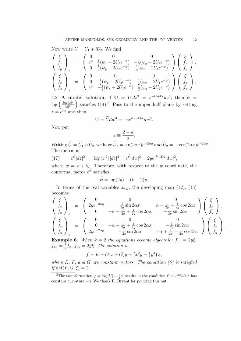
AFFINE MANIFOLDS, SYZ GEOMETRY AND THE “Y” VERTEX 12
Now write U = U1 + iU2. We find ξfxfy
x
=
0 0 0eψ 1
2(ψx + 2U1e
−ψ) −12(ψy + 2U2e
−ψ)0 1
2(ψy − 2U2e
−ψ) 12(ψx − 2U1e
−ψ)
ξfxfy
,
ξfxfy
y
=
0 0 00 1
2(ψy − 2U2e
−ψ) 12(ψx − 2U1e
−ψ)eψ −1
2(ψx + 2U1e
−ψ) 12(ψy + 2U2e
−ψ)
ξfxfy
.
4.2. A model solution. If U = U dz3 = z−(1+k) dz3, then ψ =
log(| log |z|2||z|k
)satisfies (14).3 Pass to the upper half plane by setting
z = eiw and then
U = Udw3 = −iei(2−k)wdw3.
Now put
α ≡ 2− k2
.
Writing U = U1+iU2, we have U1 = sin(2αx)e−2αy and U2 = − cos(2αx)e−2αy.The metric is
(17) eψ|dz|2 = | log |z|2| |dz|2 = eψ|dw|2 = 2ye(k−2)y|dw|2,where w = x + iy. Therefore, with respect to the w coordinate, the
conformal factor eψ satisfies
ψ = log(2y) + (k − 2)y.
In terms of the real variables x, y, the developing map (12), (13)becomes ξ
fxfy
x
=
0 0 02ye−2αy 1
2ysin 2αx α− 1
2y+ 1
2ycos 2αx
0 −α + 12y
+ 12y
cos 2αx − 12y
sin 2αx
ξfxfy
,
ξfxfy
y
=
0 0 00 −α + 1
2y+ 1
2ycos 2αx − 1
2ysin 2αx
2ye−2αy − 12y
sin 2αx −α + 12y− 1
2ycos 2αx
ξfxfy
.
Example 6. When k = 2 the equations become algebraic: fxx = 2yξ,fxy = 1
yfx, fyy = 2yξ. The solution is
f = E + (Fx+G)y +(x2y + 1
3y3)ξ,
where E, F, and G are constant vectors. The condition (5) is satisfiedif det(F,G, ξ) = 2.
3The transformation ϕ = log |U | − 12ψ results in the condition that e2ϕ|dz|2 has
constant curvature −4. We thank R. Bryant for pointing this out.
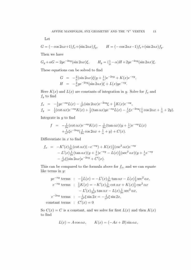
AFFINE MANIFOLDS, SYZ GEOMETRY AND THE “Y” VERTEX 13
Let
G = (− cos 2αx+1)fx+(sin 2αx)fy, H = (− cos 2αx−1)fx+(sin 2αx)fy.
Then we have
Gy+αG = 2ye−2αy(sin 2αx)ξ, Hy = ( 1y−α)H+2ye−2αy(sin 2αx)ξ.
These equations can be solved to find
G = − 2α
(sin 2αx)ξ(y + 1α
)e−2αy +K(x)e−αy,
H = − 2αye−2αy(sin 2αx)ξ + L(x)ye−αy.
Here K(x) and L(x) are constants of integration in y. Solve for fx andfy to find
fx = −12ye−αyL(x)− 1
α2 (sin 2αx)e−2αyξ + 12K(x)e−αy,
fy = 12(cotαx)e−αyK(x) + 1
2(tanαx)ye−αyL(x)− 1
αξe−2αy( 1
αcos 2αx + 1
α+ 2y).
Integrate in y to find
f = − 12α
(cotαx)e−αyK(x)− 12α
(tanαx)(y + 1α
)e−αyL(x)
+ 1α2 ξe
−2αy( 12α
cos 2αx + 1α
+ y) + C(x).
Differentiate in x to find
fx = −K ′(x) 12α
(cotαx)(−e−αy) +K(x)12(csc2 αx)e−αy
− L′(x) 12α
(tanαx)(y + 1α
)e−αy − L(x)12(sec2 αx)(y + 1
αe−αy
− 1α2 ξ(sin 2αx)e−2αy + C ′(x).
This can be compared to the formula above for fx, and we can equatelike terms in y:
ye−αy terms : −12L(x) = −L′(x) 1
2αtanαx− L(x)1
2sec2 αx,
e−αy terms : 12K(x) = −K ′(x) 1
2αcotαx +K(x)1
2csc2 αx
− L′(x) 12α2 tanαx− L(x) 1
2αsec2 αx,
e−2αy terms : − 1α2 ξ sin 2x = − 1
α2 ξ sin 2x,
constant terms : C ′(x) = 0
So C(x) = C is a constant, and we solve for first L(x) and then K(x)to find
L(x) = A cosαx, K(x) = (−Ax+B) sinαx,
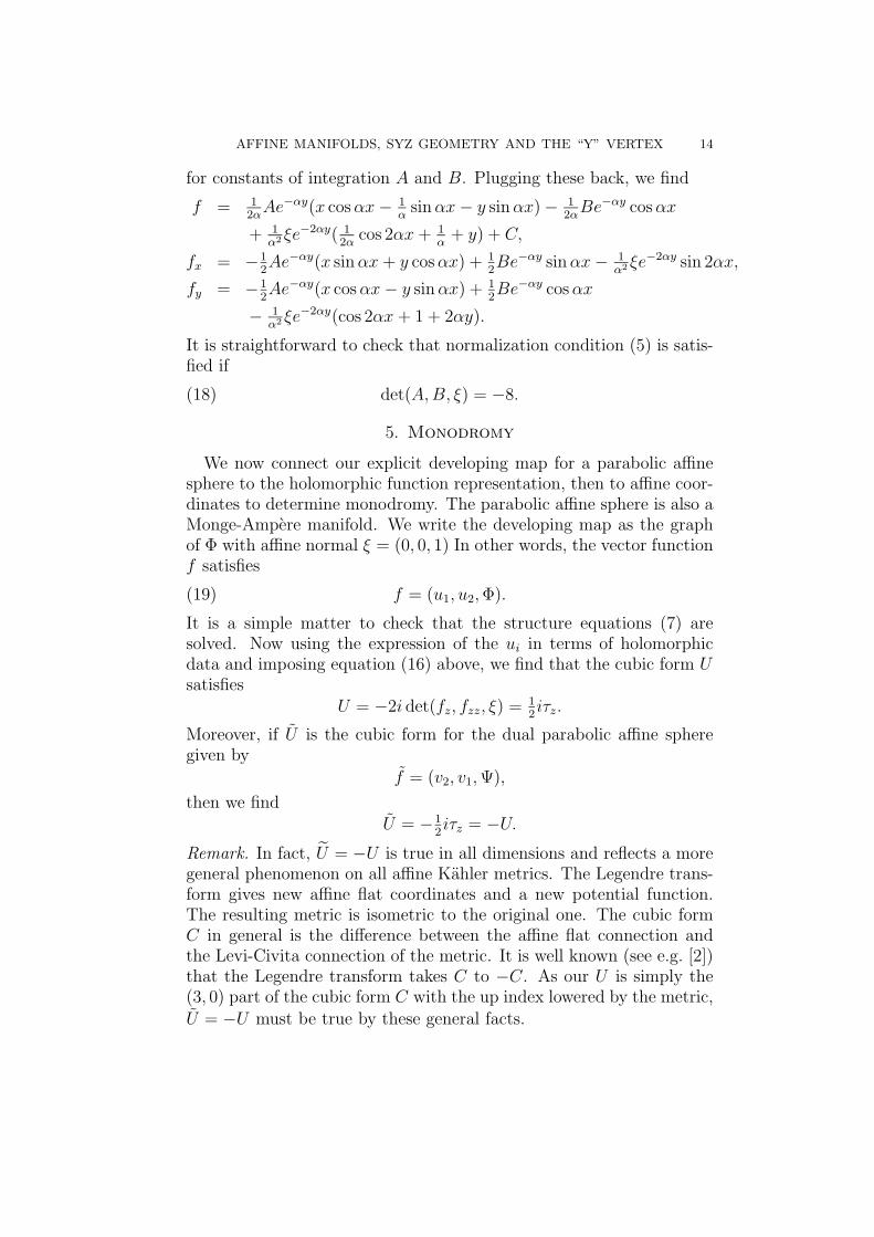
AFFINE MANIFOLDS, SYZ GEOMETRY AND THE “Y” VERTEX 14
for constants of integration A and B. Plugging these back, we find
f = 12αAe−αy(x cosαx− 1
αsinαx− y sinαx)− 1
2αBe−αy cosαx
+ 1α2 ξe
−2αy( 12α
cos 2αx + 1α
+ y) + C,
fx = −12Ae−αy(x sinαx + y cosαx) + 1
2Be−αy sinαx− 1
α2 ξe−2αy sin 2αx,
fy = −12Ae−αy(x cosαx− y sinαx) + 1
2Be−αy cosαx
− 1α2 ξe
−2αy(cos 2αx + 1 + 2αy).
It is straightforward to check that normalization condition (5) is satis-fied if
(18) det(A,B, ξ) = −8.
5. Monodromy
We now connect our explicit developing map for a parabolic affinesphere to the holomorphic function representation, then to affine coor-dinates to determine monodromy. The parabolic affine sphere is also aMonge-Ampere manifold. We write the developing map as the graphof Φ with affine normal ξ = (0, 0, 1) In other words, the vector functionf satisfies
(19) f = (u1, u2,Φ).
It is a simple matter to check that the structure equations (7) aresolved. Now using the expression of the ui in terms of holomorphicdata and imposing equation (16) above, we find that the cubic form Usatisfies
U = −2i det(fz, fzz, ξ) = 12iτz.
Moreover, if U is the cubic form for the dual parabolic affine spheregiven by
f = (v2, v1,Ψ),
then we findU = −1
2iτz = −U.
Remark. In fact, U = −U is true in all dimensions and reflects a moregeneral phenomenon on all affine Kahler metrics. The Legendre trans-form gives new affine flat coordinates and a new potential function.The resulting metric is isometric to the original one. The cubic formC in general is the difference between the affine flat connection andthe Levi-Civita connection of the metric. It is well known (see e.g. [2])that the Legendre transform takes C to −C. As our U is simply the(3, 0) part of the cubic form C with the up index lowered by the metric,U = −U must be true by these general facts.
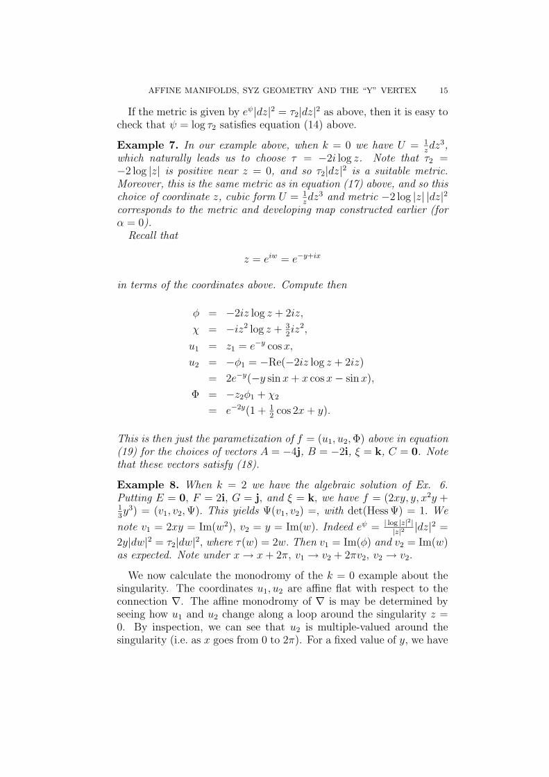
AFFINE MANIFOLDS, SYZ GEOMETRY AND THE “Y” VERTEX 15
If the metric is given by eψ|dz|2 = τ2|dz|2 as above, then it is easy tocheck that ψ = log τ2 satisfies equation (14) above.
Example 7. In our example above, when k = 0 we have U = 1zdz3,
which naturally leads us to choose τ = −2i log z. Note that τ2 =−2 log |z| is positive near z = 0, and so τ2|dz|2 is a suitable metric.Moreover, this is the same metric as in equation (17) above, and so thischoice of coordinate z, cubic form U = 1
zdz3 and metric −2 log |z| |dz|2
corresponds to the metric and developing map constructed earlier (forα = 0).
Recall that
z = eiw = e−y+ix
in terms of the coordinates above. Compute then
φ = −2iz log z + 2iz,
χ = −iz2 log z + 32iz2,
u1 = z1 = e−y cosx,
u2 = −φ1 = −Re(−2iz log z + 2iz)
= 2e−y(−y sin x+ x cosx− sin x),
Φ = −z2φ1 + χ2
= e−2y(1 + 12
cos 2x+ y).
This is then just the parametization of f = (u1, u2,Φ) above in equation(19) for the choices of vectors A = −4j, B = −2i, ξ = k, C = 0. Notethat these vectors satisfy (18).
Example 8. When k = 2 we have the algebraic solution of Ex. 6.Putting E = 0, F = 2i, G = j, and ξ = k, we have f = (2xy, y, x2y +13y3) = (v1, v2,Ψ). This yields Ψ(v1, v2) =, with det(Hess Ψ) = 1. We
note v1 = 2xy = Im(w2), v2 = y = Im(w). Indeed eψ = | log |z|2||z|2 |dz|
2 =
2y|dw|2 = τ2|dw|2, where τ(w) = 2w. Then v1 = Im(φ) and v2 = Im(w)as expected. Note under x→ x+ 2π, v1 → v2 + 2πv2, v2 → v2.
We now calculate the monodromy of the k = 0 example about thesingularity. The coordinates u1, u2 are affine flat with respect to theconnection ∇. The affine monodromy of ∇ is may be determined byseeing how u1 and u2 change along a loop around the singularity z =0. By inspection, we can see that u2 is multiple-valued around thesingularity (i.e. as x goes from 0 to 2π). For a fixed value of y, we have
AFFINE MANIFOLDS, SYZ GEOMETRY AND THE “Y” VERTEX 16
in the x, y coordinates.
f(0, y) = (0, e−y, e−2y(32
+ y)),
f(2π, y) = (4πe−y, e−y, e−2y(32
+ y)),
fx(0, y) = (−2ye−y, 0, 0),
fx(2π, y) = (−2ye−y, 0, 0),
fy(0, y) = (0,−e−y,−2e−2y(1 + y)),
fy(2π, y) = (−4πe−y,−e−y,−2e−2y(1 + y)).
The monodromy of the connection ∇ around a loop around the sin-gularity at z = 0 is computed by integrating the initial value problemto find f = (u1, u2,Φ). Let dev = (u1, u2) (this is the developing mapof the affine flat structure—see e.g. [20]). In the w coordinates, thismeans to calculate how dev changes as x 7→ x + 2π. In general, thereis a coordinate change
dev 7→M dev +N
for M ∈ GL(2,R), N ∈ R2. Differentiate this coordinate change interms of x and y, and then plug in at some point (0, y), y 0, to findthe equations
dev(2π, y) = M dev(0, y) +N,
devx(2π, y) = M devx(0, y),
devy(2π, y) = M devy(0, y).
The computations above imply that
M =
(1 2π
y
0 1
), N =
(00
).
This action is simpler in the coordinates ui. If we define ∂i ≡ ∂∂ui
then under x 7→ x + 2π, y 7→ y, we find ∂1 7→ ∂1 − 4π∂2, ∂2 7→ ∂2,the linear part of the monodromy given by an SL(2,Z) matrix. Thetranslation part (represented by N above) is 0.
6. A Radial Model for Parabolic Affine Spheres
In this section we generalize the model of Baues and Cortes for par-abolic affine spheres to two other cases. Recall the standard parabolicaffine sphere has potential Φ = ‖x‖2/2 and can be thought of in termsof a cone over the standard elliptic affine sphere ‖x‖ = 1. Baues andCortes show that this can be done with any elliptic affine sphere.
AFFINE MANIFOLDS, SYZ GEOMETRY AND THE “Y” VERTEX 17
The first generalization still involves a cone over an elliptic affinesphere. For the standard elliptic affine sphere, we recover the radiallysymmetric model in Rn+1 (3)
Φ =
∫(rn+1 + 1)
1n+1dr.
We present an analogue of this for any elliptic affine sphere.The second generalization is for part of a cone (for radial coordinate
r close to 0) over a hyperbolic affine sphere of even dimension. (Wewant the hyperbolic affine sphere to have dimension 2, so the ambientspace has dimension 3.)
The motivation for this section is to find more local models of para-bolic affine spheres in dimension 3. It may take considerable flexibilityof the local models in order to piece together appropriate global modelsof parabolic affine spheres on an affine structure on S3 minus singular-ities.
The model for these calculations may be found in [18].Consider an affine Kahler metric
gij dxidxj =
∂2Φ
∂xi∂xjdxidxj
on a domain in Rn+1. Let
X = xi∂
∂xi
be the radial vector field. Assume the metric potential Φ satisfies theansatz
(20) xi∂Φ
∂xi= XΦ = f(Φ).
This will ensure that under gij, the hypersurfaces Φ = c are orthog-onal to the radial direction X.
Apply ∂∂xj
to (20) to get
(21) xi∂2Φ
∂xi∂xj=
[df
dΦ− 1
]∂Φ
∂xjfor j = 1, . . . , n.
Consider a vector Y tangent to the hypersurface Hc = Φ = c. (SoY Φ = 0.) Then (21) shows that
g(X, Y ) = xi∂2Φ
∂xi∂xjyj =
[df
dΦ− 1
]∂Φ
∂xjyj =
[df
dΦ− 1
]Y Φ = 0,
and also
g(X,X) = xi∂2Φ
∂xi∂xjxj =
[df
dΦ− 1
]XΦ = f
[df
dΦ− 1
].
AFFINE MANIFOLDS, SYZ GEOMETRY AND THE “Y” VERTEX 18
Now we’ll show that the g restricts to a constant multiple of thecentroaffine metric on Hc.
Let D be the canonical flat connection on Rn+1. Then our affineKahler metric g is given by
(22) g(A,B) = (DAdΦ, B)
where A,B are vectors and (· , ·) is the pairing between one forms andvectors. Assume X is transverse to Hc. So at x ∈ Hc, R
n+1 = Tx(Rn+1)
splits into Tx(Hc)⊕ 〈X〉. Then we have
(23) DYZ = ∇YZ + h(Y, Z)X
where Y, Z are tangent vectors to Hc, ∇ is a connection on T (Hc), andthe centroaffine second fundamental form h is a symmetric (0, 2) tensoron Hc.
Now consider
0 = Y (dΦ, Z)
= (dΦ, DYZ) + (DY dΦ, Z)
= f h(Y, Z) + g(Y, Z)
by (20), (22) and (23). Therefore, g(Y, Z) = −f h(Y, Z) for Y, Z tan-gent to Hc. All together we have
Proposition 1. Under the metric g, each level set of the potential Φis perpendicular to the radial direction X. Furthermore,
g(X,X) = f
[df
dΦ− 1
], g(Y, Z) = −f h(Y, Z),
where Y and Z are tangent to Hc and h is the centroaffine secondfundamental form of Hc.
It is useful to introduce a radial parameter r. Let H = H1 and foliatea region in Rn+1 by ⋃
r>0
rH.
Our ansatz (20) implies that the potential Φ = Φ(r) and
(24)dΦ
dr=
1
rXΦ =
f
r,
and that each rH is a level set of Φ.Choose a basis of tangent vectors Yini=1 to H so that
(25) det(X,Y1, . . . , Yn) = 1.
AFFINE MANIFOLDS, SYZ GEOMETRY AND THE “Y” VERTEX 19
We are interested in the case g is a parabolic affine sphere metric. Inother words, we require for a positive constant k,
k = det1≤i,j≤n+1
gij
= g(X,X) det1≤i,j≤n
g(Yi, Yj)
= f
[df
dΦ− 1
](−f)n det
1≤i,j≤nh(Yi, Yj)(26)
This is because (25) and Proposition 1.We will solve this differential equation for f as a function of r. To
achieve this, we need to see how deth(Yi, Yj) scales. Let X denote the
position vector for a point in H = H1. Then X = rX is on anotherlevel set Hc, and if Yi = r−
1nYi S, then X, Yi satisfy (25). (The scaling
transformation S : X 7→ 1rX.) Then plug into (23)
DYiYj = (Yi, dYj)
= r−2n (Yi,S∗dYj)
= r−n+2n DYiYj
= r−n+2n [∇YiYj + h(Yi, Yj)X]
= r−n+2n ∇YiYj + r−
2n+2n h(Yi, Yj)X
Therefore, h(Yi, Yj) = r−2n+2n h(Yi, Yj) and
det1≤i,j≤n
h(Yi, Yj) = r−2n−2 det1≤i,j≤n
h(Yi, Yj).
Our differential equation is then
Kr2n+2 = fn+1
[df
dΦ− 1
]= fn+1
[df
dr
/dΦ
dr− 1
]= rfn
df
dr− fn+1
by (24). On H = H1, K is the constant (−1)nk/ deth(Yi, Yj). K isconstant on H by (26), and we extend K to be constant on the wholecone
⋃r>0 rH. We have taken care of the scaling by using the factor
r2n+2.If f = r2ψ then the equation is
ψn+1 + rψndψ
dr= K,
AFFINE MANIFOLDS, SYZ GEOMETRY AND THE “Y” VERTEX 20
which can be solved so that for a real constant A,
ψ =(K + Ar−n−1
) 1n+1 ,
f = r2(K + Ar−n−1
) 1n+1 ,
Φ =
∫r(K + Ar−n−1
) 1n+1 dr(27)
=
∫ (Krn+1 + A
) 1n+1 dr.
So far we’ve just dealt with the radial direction. Now we see whatconditions this ansatz imposes on the hypersurfaces Hc. We are inter-ested near the origin (as r → 0+).
Since g(Y, Z) = −f h(Y, Z), then we must require the centroaffinesecond fundamental form h to be definite in order for g to be positivedefinite. This means that the hypersurfaces Hc must be locally strictlyconvex. If Hc points away from the origin (i.e. if the origin and thehypersurface are on opposite sides of the tangent plane), then h ispositive definite. If Hc points toward the origin (i.e. if the origin andthe hypersurface are on the same side of the tangent plane), then h isnegative definite.
We apply the technique in Nomizu-Sasaki [22, p. 45] to show that Xis a multiple of the affine normal and therefore Hc is an affine sphere.The technique gives a formula for constructing the affine normal ξ toa hypersurface Hc given a transverse vector field X. We will find afunction φ and a tangent vector field W so that ξ = φX + W . Thetechnique is this: First compute
φ =
∣∣∣∣ det1≤i,j≤n
(h(Yi, Yj))
∣∣∣∣ 1n+2
=
∣∣∣∣∣kf−n−1
[df
dΦ− 1
]−1∣∣∣∣∣
1n+2
for Yi chosen as above in (25). Then—since the transverse vector fieldX is equiaffine—we have
(28) W = wi∂
∂ti= −hij ∂φ
∂tj∂
∂ti= 0.
Here hij is the inverse matrix of the second fundamental form hij =h(∂∂ti, ∂∂tj
)as in (23). The formula follows since φ is constant on Hc.
Therefore, the affine normal ξ = φX and Hc is a proper affine sphere.Assuming it’s locally strictly convex, it is an elliptic affine sphere if it
AFFINE MANIFOLDS, SYZ GEOMETRY AND THE “Y” VERTEX 21
points toward the origin and a hyperbolic affine sphere if it points awayfrom the origin.
Now consider different cases for signs of A in our exact solution (27)above. To evaluate the metric we will need below
g(X,X) = f
[df
dΦ− 1
]= f
[df
dr
/dΦ
dr− 1
]= f
[2K + Ar−n−1
K + Ar−n−1− 1
]= r2K(K + Ar−n−1)−
nn+1 .
Case 1: A > 0. In this case as r → 0+, f > 0, g(X,X) > 0 as longas K > 0, and
g(Y, Z) = −f h(Y, Z).
Therefore, we must have h negative definite (which makes K > 0). Inthis case, the hypersurface H points toward the origin and we have anelliptic affine sphere.
Example 9. For the standard elliptic affine sphere H = ‖x‖ = r =1, this example is the radially symmetric example (3).
Case 2: A = 0. In this case
g(Y, Z) = −r2K1
n+1 h(Y, Z), g(X,X) = r2K1
n+1 .
So we must have K = (−1)nk/ deth(Yi, Yj) > 0 and h negative definite(which implies K > 0). So then the Hc are elliptic affine spheres. Thisis the case that Baues and Cortes did.
Example 10. The standard parabolic affine sphere comes from thepotential Φ = 1
2‖x‖2 = 1
2
∑(xi)2. In this case we have
gij = δij,
H = ‖x‖2 = 2,
Φ =1
2r2,
f = 2Φ = r2,
k = 1,
K = 1,
g(X,X) = 2Φ = r2.
We may easily check that this example satisfies all the equations above.
AFFINE MANIFOLDS, SYZ GEOMETRY AND THE “Y” VERTEX 22
To be concrete, a function u : Rn → R obeying det (Hess(u)) =u−(n+2) determines an elliptic affine sphere, S, given by x 7→ y(x) =(x, u(x)). Then the mapping (r, x) 7→ y(r, x) = (rx, ru(x)) is locallyinvertible and thus we can write r = r(y). Then Φ(y) = r(y)2/2 is aHessian potential for a parabolic affine sphere (i.e. det (Hess(Φ)) = 1)with cone metric over S. In the (r, x) coordinates we have ds2 = dr2 +r2uijdx
idxj, a cone over S.
Case 3: A < 0. In this case as r → 0+, we must have n even in orderfor (27) to make sense. (We are interested in the case n = 2.) Thenwe must have
K = (−1)nk/ deth(Yi, Yj) > 0
to make g(X,X) > 0. For n even, this happens when h is eitherpositive or negative definite. Also, f < 0 for r → 0+. Therefore,g(Y, Z) = −f h(Y, Z) implies that h must be positive definite. In otherwords, H points away from the origin and is a hyperbolic affine sphere.
Example 11. For this case, consider n = 2 and the standard hyperbolicaffine sphere in R3
H = x3 =√
1 + (x1)2 + (x2)2.
Then r =√
(x3)2 − (x1)2 − (x2)2. Let A = −1 and K = 1. Then
Φ =
∫ (r3 − 1
) 13 dr.
Compute the metric gij =∂2Φ
∂xi∂xjto be
1
r3(r3 − 1)23
−r5 + r2 + (x1)2 x1x2 −x1x3
x1x2 −r5 + r2 + (x2)2 −x2x3
−x1x3 −x2x3 r5 − r2 + (x3)2
.
It is straightforward to check that det gij = 1. Also,
g(X,X) = r2(1− r−3)−23 , g(Y, Z) = −r2(1− r−3)
13 h(Y, Z).
So this metric is positive definite only for 0 < r < 1. It is incompleteas r → 0 and as r → 1.
7. Elliptic Affine Spheres and the “Y” Vertex
In this section we will prove the existence of elliptic affine two-spheremetrics with singularities – first locally near a singularity, then globallyon S2 minus three points. The metric cone yields a parabolic affinesphere metric near the “Y” vertex.
AFFINE MANIFOLDS, SYZ GEOMETRY AND THE “Y” VERTEX 23
7.1. Local Analysis. It is a simple matter to mimic the constructionof section 4 in the case of an elliptic affine sphere, for which the normalvector can be taken to point to the origin: ξ = −f. The second struc-ture equation in (7) is then DXξ = −f∗X. With this modification, theintegrability condition (Eq. (14)) becomes Uz = 0 and
(29) ψzz + |U |2e−2ψ +1
2eψ = 0.
Since we can construct a parabolic affine sphere on the cone over an el-liptic sphere, a solution to this equation on the thrice-punctured spherewill lead to a parabolic affine sphere on R3 minus a Y-shaped set –whence a semiflat special Lagrangian torus fibration over this base.We will prove that a solution ψ exists to Eq. (29) in a certain functionspace. This will allow us to study monodromy, as in section 5. Wethen discuss the more global setting of the thrice-punctured sphere.
For definiteness, we consider the case U = z−2 and make the ansatzψ = ψ(|z|). We look near z = 0, so we make the change of variablest = − log |z|, t ∈ (T,∞), T 0. This leads to the equation
(30) N(ψ) := ∂2t ψ + 4e−2(ψ−t) + 2eψ−2t = 0.
We put ψ = ψ0 + φ, where ψ0 = t + log(2t) is the solution to theparabolic equation (14). Note that the last term is O(te−t) for thisfunction. We want to solve N(ψ0 + φ) = 0, which we expand as
(31) N(ψ0 + φ) = N(ψ0) + dN(φ)|ψ0 +Q(φ)|ψ0 ,
where Q(φ) contains quadratic and higher terms. Explicitly,
Q(φ) =1
t2(e−2φ − (1− 2φ)
)+ 4te−t
(eφ − (1 + φ)
).
Note that Q is not even a differential operator. One calculates
N(ψ0) = 4te−t,
dN(φ)|ψ0 =: Lφ :=[∂2t + V (ψ0)
]φ,
where
V (ψ0) = −8e−2(ψ0−t) + 2eψ0−2t = − 2
t2+ 4te−t.
Thus Lφ = (∂2t − 2
t2+ 4te−t)φ = (L0 + 4te−t)φ, where L0 = ∂2
t − 2t2.
The equation (29) is now
Lφ = f −Q(φ),
with f = −4te−t. The idea will be to find an appropriate Green functionG for L, in terms of which a solution to this equation becomes a fixedpoint of the mapping φ → G(f − Q(φ))—then to find a range of φ

AFFINE MANIFOLDS, SYZ GEOMETRY AND THE “Y” VERTEX 24
where this is a contraction map, whence a solution by the fixed pointtheorem.
We claim that this map is a contraction for φ ∼ O(te−t). Morespecifically, consider for a value of T > 2 to be determined later, theBanach space B of continuous functions on [T,∞) with norm
‖f‖B = supt≥T
f(t)
te−t.
Showing the map φ → G(f − Q(φ)) is a contraction map involvesestimating Gf and GQφ. In fact, since Q is a quadratic, nonderivativeoperator, it is easy to see that Qφ is order te−t (even smaller). Wethen show that G preserves the condition O(te−t) by showing Gf ∈ B(recall that f ∈ B, too). To find G, we write L = L0 − δL, whereδL = −4te−t, so that G = L−1 = L−1
0 + L−10 δLL
−10 + .... To solve the
equation Lu = f, we first note that the change of variables v = u + 1leads to the equation Lv = − 2
t2. Let v0 = L−1
0 (− 2t2
) = 1. Then define
vk+1 = L−10 δLvk. Then v =
∑∞k=0 vk and Gf = u =
∑∞k=1 vk.
Lemma 2. |vk(t)| < (16te−t)k pointwise.
Proof. It is true for k = 0. To compute vk+1 one solves the differ-ential equation by the method of variation of parameters,4 using thehomogeneous solution t2 or t−1. We have
vk+1(t) = t2∫ ∞t
t−41
∫ ∞t1
t22(−4t2e−t2vk(t2)dt2dt1.
One computes v1(t) = −4(t+2+2/t)e−t, and therefore |v1(t)| < 16te−t
for t > 2. Now assume |vk(t)| < (16te−t)k for some k ≥ 1. Firstcompute for a, b ∈ N, t > a/b and t > 2:∫ ∞
t
sae−bsds = −1
b
[sa +
a
bsa−1 +
a(a− 1)
b2sa−2 + ...
]e−bs
∣∣∣∣∞t
≤ 1
bta(1 + (a/bt) + (a/bt)2 + ...)e−bt
≤ t
b(t− 1)tae−bt ≤ 2tae−bt.
4We can write G0h(t) =∫∞TK0(t, s)h(s)ds, where K0(t, s) = 1
3 ( s2
t −t2
s ) fors > t and zero otherwise (this form of the kernel is relevant to the condition ofgood functional behavior at infinity). One can also use the equivalent G0h(t) =t2∫∞tt−41
∫∞t1s2h(t2)dt2dt1, which appears in the text.
AFFINE MANIFOLDS, SYZ GEOMETRY AND THE “Y” VERTEX 25
Therefore,
|vk+1(t)| ≤ 4t2∫ ∞t
t−41
∫ ∞t1
t32e−t2vk(t2)dt2dt1
≤ 4t2∫ ∞t
t−41
∫ ∞t1
t32e−t2(16)ktk2e
−kt2dt2dt1
≤ (16)k · 4 · 2t2∫ ∞t
tk+3−41 e−(k+1)t1dt1
≤ (16)k+1tk+1e−(k+1)t
and the lemma is proven.5 It now follows that u < C(1 − 4te−t)−14te−t ≤ C ′te−t for some
constant C ′. The space S = f(t) : |f(t)| ≤ 2C ′te−t forms a closedsubset of B on which we apply the contraction mapping theorem.
Proposition 3. There is a constant T > 0 so that for t ≥ T , theequation (29) has a solution of the form log(2t) + t+O(te−t).
Proof. We now show the mapping φ → Aφ ≡ Gf − GQφ is acontraction. First, Gf lies within S and Qφ is small since Q is aquadratic nondifferential operator. More specifically, for some T > 0,the sup norm of φ on [T,∞) can be made arbitrarily small. Therefore,on [T,∞), ‖Qφ‖B ‖φ‖B. As a result, A maps S to S. Further, note‖Aφ1 − Aφ2‖B = ‖GQφ1 − GQφ2‖B = ‖G(Qφ1 − Qφ2)‖B, since G islinear. Since Q is quadratic and φ is small, ‖Qφ1−Qφ2‖B ‖φ1−φ2‖B,and A is a contraction since in the operator norm ‖G‖ < C ′/4 by theprevious lemma. Thus we can clearly find a T > 0 so that for a fixedθ < 1, ‖Aφ1 −Aφ2‖B ≤ θ‖φ1 − φ2‖B for φ1, φ2 ∈ S. By the fixed pointtheorem, there exists φ such that Aφ = φ. φ is smooth by standardbootstrapping. Then log(2t) + t+ φ(t) solves (29).
In the next section, we will require the local form of our global func-tion to be consistent with the log | log |z|2|−log |z|+O(|z| log |z|) behav-ior of this local solution. The dominant term is − log |z| which comesfrom the form of U and determines the residue at the singularity.
7.2. Global Existence. The coordinate-independent version of Eq.(29) for a general background metric, is
(32) ∆u+ 4‖U‖2e−2u + 2eu − 2κ0 = 0
on S2, where norms, gradients, integrals, etc., are taken with respectto the background metric. U is a holomorphic cubic differential, whichwe take to have exactly 3 poles of order 2 and thus no zeroes, and u is
5Note that we needed k − 1 ≥ 0 to bound a/b from above. That the k = 1 termis the proper order follows from some fortuitous cancellation.
AFFINE MANIFOLDS, SYZ GEOMETRY AND THE “Y” VERTEX 26
taken to have a prescribed singularity structure such that∫
∆u = 6π,which follows from our local analysis in Section 7.1.
Near each pole of U , there is a local coordinate z so that the poleis at z = 0, and U = z−2dz3 exactly. We call this z the canonicalholomorphic coordinate. In a neighborhood of each pole, we take
(33) u0 = log | log |z|2| − log |z|
and the background metric to be |dz|2. The background metric and u0
are extended smoothly to the rest of CP1. Note that∫
∆u0 = 6π (eachpole contributes 2π). All integrals in this section will be evaluated withrespect to the background metric.
To implement the required singularity structure, we write u = u0 +ηfor η in the Sobolev space H1. Note this implies
∫∆η = 0. We define
the functional
(34)J(η) =
∫ (12|∇η|2 + (2κ0 −∆u0)η + 1
23 · 4‖U‖2e−2u0e−2η
)−2π log
∫(4‖U‖2e−2u0e−2η + 2eu0eη) .
(We note that it is necessary to separate η from u0 as ∇u0 is not in L2.)J is not defined for all functions η ∈ H1. One problem is that ∆u0 /∈ L2.The term
∫∆uoη can be taken care of by integrating by parts (see
the proof of Proposition 5 below). A more serious problem is that4‖U‖2e−2u0 /∈ Lp for any p > 1. This cannot be fixed by integratingby parts, as the example η = −1
2log | log |z|2| ∈ H1,loc shows. That
said, there is a uniform lower bound on J among all η ∈ H1 so that∫4‖U‖2e−2u0e−2η < ∞ (see the remark after Proposition 5). Thus
we can still talk of taking sequences of η ∈ H1 to minimize J . (Theterm
∫2eu0eη is always finite for η ∈ H1 since eu0 ∈ Lp for p < 2 and
Moser-Trudinger shows that eη ∈ Lq for all q <∞.)We wish to show that J(η) has a minimum. If so, then the minimum
satisfies the Euler-Lagrange equation(35)
∆η−(2κ0−∆u0)+3·4‖U‖2e−2u0e−2η+−2 · 4‖U‖2e−2u0e−2η + 2eu0eη
12π
∫4‖U‖2e−2u0e−2η + 2eu0eη
= 0.
One can easily check by integrating this equation that for a solution η0,the denominator in the last term must be equal to one. Thus u = η0+u0
satisfies the original equation (32). In this case, the equation η0 satisfiesis
(36) ∆η − (2κ0 −∆u0) + 4‖U‖2e−2u0e−2η + 2eu0eη = 0.
AFFINE MANIFOLDS, SYZ GEOMETRY AND THE “Y” VERTEX 27
This is equivalent to equation (29), the equation for the metric of anelliptic affine sphere: for the background metric h, write eu0+ηh =eψ|dz|2. Then η satisfies (36) if and only if ψ satisfies (29).
Definition 1. We call η admissible if η ∈ H1 and∫
4‖U‖2e−2u0e−2η <∞.
In order to analyze the functional J , for an admissible η, considerJ(η + k) for k a constant. J(η + k) has the form
(indep. of k) + 2πk + 3πAe−2k − 2π log[2π(Ae−2k +Bek)],
where
(37) A = A(η) ≡ 1
2π
∫4‖U‖2e−2u0e−2η, B = B(η) ≡ 1
2π
∫2eu0eη.
Thus upon setting (∂/∂k)J(η + k) = 0, we find a critical point only ifAe−2k +Bek = 1, and this can only happen if
AB2 ≤ 4
27.
If AB2 > 4/27, then the infimum occurs as k → +∞, and if AB2 <4/27, there are two finite critical points: a local minimum for whichB(η+k) = Bek < 2/3 and a local maximum for which B(η+k) > 2/3.With that in mind, we formulate the following variational problem:
LetQ = η ∈ H1 : A+B ≤ 1.
We will minimize J for η ∈ Q. Note that this will avoid the potentialproblem at k → +∞, where B(η + k) → +∞. Also, the inequalityin the definition of Q will be important. It will allow us to use theKuhn-Tucker conditions to control the sign of the Lagrange multiplierin the Euler-Lagrange equations. The discussion above about addinga constant k can be summarized in
Lemma 4. If η ∈ Q, then the minimizer of
J(η + k) : k constant, η + k ∈ Qoccurs for k so that A(η+k)+B(η+k) = 1, B(η+k) ≤ 2/3, and k ≤ 0.If A(η) + B(η) < 1, then the minimizer k < 0 and B(η + k) < 2/3.Moreover, if A(η) +B(η) = 1 and B(η) ≤ 2/3, then k = 0.
Proof. Compute (∂/∂k)J(η + k) and use the first derivative test.
Proposition 5. There are positive constants γ and R so that for allη ∈ Q,
J(η) ≥ γ
∫|∇η|2 −R.
AFFINE MANIFOLDS, SYZ GEOMETRY AND THE “Y” VERTEX 28
Remark. We can also prove the same result for all admissible η ∈ H1.In this case, we must also control potential minimizers at k = +∞.For admissible ρ ∈ H1 so that
∫ρ = 0, consider the functional
J(ρ) = limk→∞
J(ρ+ k).
We bound J from below much the same as the following argument,although there also is an extra term in J that must be handled usingthe Moser-Trudinger estimate.
Proof. As above, u0 = log | log |z|2|− log |z| in the canonical coordinatez near each pole of U . Since ∆u0 /∈ L2, we should integrate by partsto handle the −
∫∆u0 η term in J . Let u′0 = log | log |z|2| near each
pole of U and smooth elsewhere. Then ∆u0 = ∆u′0 near each pole andthe difference ∆u0 − ∆u′0 is smooth on CP1. Then if we let ζ be thesmooth function 2κ0 −∆(u0 − u′0),
J(η) =
∫[1
2|∇η|2 + ζη −∆u′0 η] + 3πA− 2π log 2π(A+B)
>
∫[1
2|∇η|2 + ζη +∇u′0 · ∇η]− 2π log 2π
≥ C +
∫ [1
2|∇η|2 − 1
4εζ2 − εη2 − 1
4ε|∇u′0|2 − ε|∇η|2
]≥ Cε +
∫ (1
2− δ)|∇η|2
Here δ = ( 1λ1
+ 1)ε, for λ1 the first nonzero eigenvalue of the Laplacianof the background metric, and we’ve used the facts that A > 0 andA+B ≤ 1.
Here is another useful lemma.
Lemma 6. For any η ∈ H1,
AB2 ≥ L = 2π−3
(∫‖U‖
23
)3
.
If AB2 = L, then there is a constant C such that
η = C + 23
log ‖U‖ − u0.
Proof. Let f = (4‖U‖2)13 e−
23
(u0+η), g = e23
(u0+η). Apply Holder’s in-equality
∫fg ≤ ‖f‖3‖g‖ 3
2. The last statement follows from the case of
equality in Holder’s inequality.
AFFINE MANIFOLDS, SYZ GEOMETRY AND THE “Y” VERTEX 29
Remark. The bound L in the previous lemma does not depend on thebackground metric; it depends only on the conformal structure on CP1
and the cubic form U .
An admissible η ∈ H1 is a weak solution of (36) if η is a solution of(36) in the sense of distributions.
Proposition 7. Assume that U is such that L < 4/27. Then anyminimizer η of J(η) : η ∈ Q is a weak solution of (36).
Proof. Recall Q = η : A+B ≤ 1.Case 1: The minimizer η satisfies A + B < 1. Since the constraint
A + B ≤ 1 is slack, η must satisfy the Euler-Lagrange equation (35).Then as above, we may integrate to find that the denominator A + Bin (35) must be equal to 1. Thus this case cannot occur.
Case 2: The minimizer η satisfies A + B = 1. In this case, we haveLagrange multipliers [µ0, µ1] ∈ RP1 so that η weakly satisfies
µ0
[∆η − (2κ0 −∆u0) + 3 · 4‖U‖2e−2u0e−2η +
−2 · 4‖U‖2e−2u0e−2η + 2eu0eη
A+B
]= µ1(−2 · 4‖U‖2e−2u0e−2η + 2eu0eη),
and A+B = 1. Thus,
(38) µ0[∆η − (2κ0 −∆u0) + a+ b] = µ1(−2a+ b)
for
a = 4‖U‖2e−2u0e−2η, b = 2eu0eη.
Note then that A =∫a/2π, B =
∫b/2π.
Also note the constraint the Kuhn-Tucker conditions place on theLagrange multipliers. Recall that if we minimize a function f subjectto the constraint g ≤ 1, and if the minimum occurs on the boundaryg = 1, then we have µ0∇f = µ1∇g for µ0µ1 ≤ 0. This is exactly oursituation for f = J and g = A+B.
Thus we have three cases: if µ1 = 0, then equation (38) becomesequation (36) and we’ve proved the proposition.
In the second case, if µ0 = 0, then the Euler-Lagrange equation (38)may be solved explicitly for η to find
η = 13
log(4‖U‖2)− u0.
Near each pole of U , there is a coordinate z so that ‖U‖ = |z|−2 andu0 = log | log |z|2| − log |z|. So
η = 13
log 4− 13
log |z| − log | log |z|2|
there and so η /∈ H1.

AFFINE MANIFOLDS, SYZ GEOMETRY AND THE “Y” VERTEX 30
Finally, we consider where µ = µ1/µ0 < 0. We will analyze the sec-ond variation at any critical point to show that there are no minimizersin this case.
Integrate (38) to find
−2π + 2πA+ 2πB = µ(−2 · 2πA+ 2πB).
Then since A+B = 1, we have 2A = B, since we are in the case µ 6= 0.So A = 1/3 and B = 2/3. We analyze the second variation to showthat for L < 4/27, there is no minimizer at A = 1/3, B = 2/3 (unlesspossibly if µ1 = 0).
Let η satisfy (38) and A = 1/3, B = 2/3. Consider a variation
η+ εα+ ε2
2β so that η satisfies A+B = 1 to second order when ε = 0.6
We assume α is a constant. Then the first variation
∂
∂ε(A+B)
∣∣∣∣ε=0
= −2αA + αB = 0
for A = 1/3, B = 2/3. So to first order η + α satisfies A + B = 1 andα is tangent to A+B = 1.
Now we require
0 = 2π∂2
∂ε2(A+B)
∣∣∣∣ε=0
=
∫a(4α2 − 2β) + b(α2 + β)
= α22π(4A+B) +
∫β(−2a+ b)
= 2π · 2α2 +
∫β(−2a+ b).(39)
6This corresponds to an actual variation in Q by standard Implicit FunctionTheorem arguments—see [17]. Let X be the Banach space H1 ∩ C0. Then letg : X → R, g(ν) = A(η + ν) + B(η + ν). It is straightforward to show that g isC1 in the Banach space sense. Moreover, for 2a 6= b (which holds for any η ∈ H1),we can check that dg : X → R is nonzero. So then Y = g−1(1) = A + B = 1is a Banach submanifold of X near ν = 0. So for any element α ∈ ker dg0, thereis a curve in Y tangent to α. Along such a curve, we compute restrictions on thesecond-order term β.
AFFINE MANIFOLDS, SYZ GEOMETRY AND THE “Y” VERTEX 31
Now for this variation J = J(η + εα + ε2
2β), compute
∂2J
∂ε2
∣∣∣∣ε=0
=
∫∇η · ∇β + |∇α|2 + (2κ0 −∆u0)β + 3
2
∫a(4α2 − 2β)
− 2π
∫a(4α2 − 2β) + b(α2 + β)∫
a+ b+ 2π
(∫a(−2α) + bα
)2(∫a+ b
)2
=
∫[∇η · ∇β + (2κ0 −∆u0)β − 3aβ] + 2π · 6α2A
− 2π · α2(4A+B)−∫β(−2a+ b)
=
∫[∇η · ∇β + (2κ0 −∆u0)β − 3aβ] + 2π · 2α2(40)
Here we’ve used the following facts to get from the first line to thesecond: ∇α = 0 since α is constant,
∫(a + b)/2π = A + B = 1, and
the last term vanishes since α is constant and 2A = B. The third linefollows from the second by the constraint (39) and the fact A = 1/3.
Now we use the Euler-Lagrange equation (38). Recall µ0 6= 0 andµ = µ1/µ0. Then∫∇η · ∇β = −
∫(∆η)β =
∫[−(2κ0 −∆u0) + a+ b− µ(−2a+ b)]β.
Plug this into (40) to find
∂2J
∂ε2
∣∣∣∣ε=0
= (1− µ)
∫(−2a+ b)β + 2π · 2α2
= 2π · 2µα2.
Here the last line follows from (39). Thus if we choose α 6= 0, then thesecond variation along this path is negative since µ < 0. Therefore,there is no minimizer for our variational problem satisfying µ < 0.
Now we show that there is a minimizer.
Lemma 8. Assume L < 4/27. Then there is a constant δ > 0 so thatA,B ∈ (δ, 1/δ) for all η ∈ Q.
Proof. Lemma 6 implies that AB2 ≥ L. Since 0 < L < 4/27, A > 0,B > 0, and A+B ≤ 1, this proves the lemma.
Lemma 9. There are constants K1, K2 so that for all admissible η ∈H1, and for c = (
∫η)/(
∫1),
logA ≥ K1 − 2c, logB ≥ K2 + c.

AFFINE MANIFOLDS, SYZ GEOMETRY AND THE “Y” VERTEX 32
Proof. Since exp is convex, Jensen’s inequality gives
logA = − log 2π + log
∫4‖U‖2e−2u0e−2η
≥ − log 2π +
∫log 4‖U‖2 − 2u0 − 2η∫
1+ log
∫1.
The case for B is the same.
Lemma 10. Let ηi be a sequence in Q so that limi J(ηi) = infη∈Q J(η).Then there is a positive constant C so that ‖ηi‖H1 ≤ C for all i.
Proof. First we note that Lemmas 8 and 9 show that the average valuec = (
∫η)/(
∫1) is uniformly bounded above and below for all η ∈ Q.
Proposition 5 shows that J(η) ≥ γ∫|∇η|2 − R for γ,R > 0 uni-
form constants. Thus for any minimizing sequence,∫|∇η|2 must be
uniformly bounded. Then write η = ρ+c for∫ρ = 0, c constant. Then
‖η‖L2 ≤ ‖ρ‖L2 + ‖c‖L2 ≤ λ− 1
21 ‖∇ρ‖L2 +K = λ
− 12
1 ‖∇η‖L2 +K
for K a uniform constant and λ1 the first nonzero eigenvalue of theLaplacian. This shows the H1 norm of η in the minimizing sequence isuniformly bounded.
Now given a minimizing sequence ηi ⊂ Q, Lemma 4 shows thatwe can assume A(ηi) + B(ηi) = 1, B(ηi) ≤ 2/3. Then there is a sub-sequence, which we still refer to as ηi, which is weakly convergent to afunction η∞ ∈ H1 (the weak compactness of the unit ball in a Hilbertspace), strongly convergent to η∞ in Lp for p < ∞ (Sobolev embed-ding), convergent pointwise almost everywhere to η∞ (Lp convergenceimplies subsequential almost-everywhere convergence), and so that eηi
is strongly convergent to eη∞ in Lp for p <∞ (Moser-Trudinger). Re-call
J(η) =
∫[12|∇η|2 + (2κ0 −∆u0)η] + 3πA− 2π log 2π(A+B).
Then the second term in the integral converges by strong convergencein L1 and weak convergence in H1 (see the proof of Proposition 5 forthe integration by parts trick). The term
∫12|∇η|2 is lower semicontin-
uous (the norm in a Hilbert space is lower semicontinuous under weakconvergence). Lower semicontinuity is enough since we are seeking aminimizer. B converges by Moser-Trudinger: eu0 ∈ Lp for p < 2. Thensince eηi converges in Lq for 1
p+ 1
q= 1, B =
∫2eu0eη converges.
AFFINE MANIFOLDS, SYZ GEOMETRY AND THE “Y” VERTEX 33
That leaves the term A. Fatou’s lemma and the almost-everywhereconvergence of ηi then show
A(η∞) ≤ lim infi→∞
A(ηi).
We want to rule out the case of strict inequality. Note A(η∞)+B(η∞) ≤limA(ηi) + B(ηi) = 1, and so η∞ ∈ Q. Also, since A(ηi) + B(ηi) = 1and B(ηi)→ B(η∞), limA(ηi) = 1−B(η∞).
Consider the constant k so that η∞ + k minimizes
J(η∞ + k) : η∞ + k ∈ Q.Note that Lemma 4 shows that e−2kA(η∞) + ekB(η∞) = 1. Now com-pute
limi→∞
J(ηi) ≥∫ [
12|∇η∞|2 + (2κ0 + ∆u0)η∞
]+ 3π [1−B(η∞)] ,
J(η∞ + k) =
∫ [12|∇η∞|2 + (2κ0 + ∆u0)(η∞ + k)
]+ 3πe−2kA(η∞).
Now substitute e−2kA(η∞) = 1− ekB(η∞) to show
(41) limi→∞
J(ηi)− J(η∞ + k) ≥ −2πk + 3πB(η∞)(ek − 1)
We prove A(η∞) = limA(ηi) by contradiction. If on the contraryA(η∞) < limA(ηi), Lemma 4 and the fact A(ηi)+B(ηi) = 1 imply thatk < 0. Then it is straightforward to check that the right-hand side of(41) is strictly positive (it is zero if k = 0, and its derivative with respectto k is negative for k < 0—use the fact B(η∞) = limB(ηi) ≤ 2/3.) Thisshows lim J(ηi) > J(η∞ + k) and so contradicts the fact that ηi is aminimizing sequence for J .
The same analysis shows that lim∫|∇ηi|2 =
∫|∇η∞|2. So J(η∞) =
lim J(ηi), and η∞ is a minimizer of J(η) : η ∈ Q.Theorem 1. If L < 4/27 then a weak solution to (36) exists. Con-versely, if L ≥ 4/27, then there is no weak solution to (36).
Proof. The preceding paragraphs, together with Proposition 7, proveexistence in the case L < 4/27. We address the nonexistence in twocases:
Case L > 4/27. If η solves (36), then we can integrate (36) to findA + B = 1. On the other hand, A > 0, B > 0, and Lemma 6 showsthat AB2 ≥ L > 4/27. Simple calculus shows that there is no suchpair (A,B) in this case.
Case L = 4/27. As in Case 1, we must have A+ B = 1 and AB2 ≥L = 4/27. The only way this can happen is if A = 1/3, B = 2/3, so
AFFINE MANIFOLDS, SYZ GEOMETRY AND THE “Y” VERTEX 34
that AB2 = 4/27. In this case, Lemma 6 forces η = C + 23
log ‖U‖−u0
for some constant C. Since u0 = log | log |z|2| − log |z| and ‖U‖ = |z|−2
near each pole of U , η = C − log | log |z|2| − 13
log |z| near each pole ofU . Thus η /∈ H1.
Proposition 11. Any weak solution η to (36) is smooth away from thepoles of U .
Proof. In a neighborhood bounded away from the poles of U , the quan-tities ‖U‖2 and u0 are smooth and bounded. Since η ∈ H1, Moser-Trudinger shows that eη, e−2η ∈ Lp for all p < ∞. Therefore, (36)implies ∆η ∈ Lploc. Since η ∈ Lp by Sobolev embedding, the Lp elliptic
theory [10] shows that η ∈ W 2,ploc . Sobolev embedding shows η ∈ C0,α
loc ,
and so ∆η ∈ C0,αloc . The Schauder theory then shows η ∈ C2,α
loc . Furtherbootstrapping implies η is smooth.
7.3. A metric for the “Y” vertex. Let Σ be the universal cover ofΣ = S2 \ p1, p2, p3. Lifting the appropriate objects to the cover we
find a solution to (32) on Σ. Since the equation (32) is the integrability
condition for the developing map, we have a solution f : Σ→ R3, with
monodromies of Σ acting as equiaffine deck transformations fixing thenormal vector ξ and acting by isometry. The quotient by the decktransformations gives an elliptic affine sphere structure on Σ as well asthe locally defined developing map f. Then the map F : (Σ × R+) →R
3 defined by F (x, r) = rf(x) =: (y1, y2, y3) maps the cone over Σto R3 and is locally invertible (so we may express r = r(y)). Thepotential function Φ(y) = r2/2 defines a parabolic affine sphere on aneighborhood of the “Y” vertex, by the result of Baues and Cortes (seeExample 10). This is our main result.
Remark. The monodromy group of this metric determines the affine flatstructure. We have not yet determined this monodromy group, thuscannot verify that the metric is one predicted by Gross and Siebert[12].
Acknowledgments
We would like to thank Rafe Mazzeo for stimulating discussions. Thework of S.-T. Yau was supported in part by the National Science Foun-dation (DMS-0244464, DMS-0074328, DMS-0306600, DMS-9803347).The work of E. Z. was supported in part by the National Science Foun-dation (DMS-0072504) and by the Alfred P. Sloan Foundation.
AFFINE MANIFOLDS, SYZ GEOMETRY AND THE “Y” VERTEX 35
References
[1] M. Aganagic, A. Klemm, M. Marino, and C. Vafa, “The Topological Vertex,”hep-th/0305132.
[2] S. Amari and H. Nagaoka, Methods of Information Geometry, The AmericanMathematical Society, Providence, 2000.
[3] O. Baues and V. Cortes, “Proper Affine Hyperspheres which fiber over Pro-jective Special Kaehler Manifolds,” math.DG/0205308.
[4] V. Cortes, “A Holomorphic Representation formula for parabolic hypersphers,”math.DG/0107037.
[5] E. Calabi, “A Construction of Nonhomogeneous Einstein Metrics,” Proc. ofSymp. in Pure Mathematics 27, AMS, Providence (1975) 17-24.
[6] E. Calabi, “Complete Affine Hypersurfaces I,” in Symposia Mathematica X,Academic Press, London (1972) 19-38.
[7] S.-Y. Cheng and S.-T. Yau. Complete affine hyperspheres. part I. The com-pleteness of affine metrics. Communications on Pure and Applied Mathematics,39(6):839–866, 1986.
[8] S. K. Donaldson and R. P. Thomas, “Gauge Theory in Higher Dimensions,”The Geometric Universe (Oxford, 1996), Oxford Univ. Press, Oxford (1998)pp. 31-47.
[9] K. Fukaya, “Multivalued Morse Theory, Asymptotic Analysis, andMirror Symmetry,” preprint available at http://www.math.kyoto-u.ac.jp/ fukaya/fukaya.html
[10] D. Gilbarg and N. Trudinger, Elliptic Partial Differential Equations of SecondOrder, Springer-Verlag, Berlin, 1983.
[11] M. Gross, “Topological Mirror Symmetry,” Invent. Math. 144 (2001) 75–137;and “Special Lagrangian Fibrations I: Topology,” in Winter School on MirrorSymmetry, Vector Bundles and Lagrangian Submanifolds, C. Vafa and S.-T.Yau, eds., AMS/International Press (2001) 65–93.
[12] M. Gross and B. Siebert, “Affine Manifolds, Log Structures, and Mirror Sym-metry,” Turkish Journal of Mathematics 27 (2003) 33-60; “Mirror Symmetryvia Logarithmic Degeneration Data I,” math.AG/0309070.
[13] M. Gross and P. M. H. Wilson, “Large Complex Structure Limits of K3 Sur-faces,” J. Diff. Geom. 55 (2000) 475-546. math.DG/0008018.
[14] N. Hitchin, “The Moduli Space of Special Lagrangian Submanifolds,” dedi-cated to Ennio De, Ann. Scuola Norm. Sup. Pisa Cl. Sci. 25 (1997) 503–515.
[15] N. Hitchin, “Lectures on Special Lagrangian Submanifolds,”math.DG/9907034.
[16] M. Kontsevich and Y. Soibelman, “Homological Mirror Symmetry and TorusFibrations,” in Symplectic Geometry and Mirror Symmetry, World Scientific(2001) 203–263.
[17] S. Lang, Differential Manifolds, Springer-Verlag, New York, 1985.[18] J. Loftin, “Affine Spheres and Kahler-Einstein Metrics,” Math. Res. Lett. 9(4)
425–432.[19] J. Loftin, “The Compactification of the Moduli Space of RP2 Surfaces, I,”
math.DG/0311052.[20] J. Loftin, “Singular Semi-Flat Calabi-Yau Metrics on S2,” math.DG/0403218.[21] H. Ooguri and C. Vafa, “Summing up D-Instantons,” Phys. Rev. Lett. 77
(1996) 3296-3298.
AFFINE MANIFOLDS, SYZ GEOMETRY AND THE “Y” VERTEX 36
[22] K. Nomizu and T. Sasaki, Affine Differential Geometry, Cambridge UniversityPress, Cambridge, 1994.
[23] V. Ruuska, “Riemannian Polarizations,” Ann. Acad. Sci. Fenn. Math. Diss.,106 (1996), 38 pp.
[24] U. Simon and C.-P. Wang. Local theory of affine 2-spheres. In DifferentialGeometry: Riemannian geometry (Los Angeles, CA, 1990), volume 54-3 ofProceedings of Symposia in Pure Mathematics, pages 585–598. American Math-ematical Society, 1993.
[25] A. Strominger, S.-T. Yau, and E. Zaslow, “Mirror Symmetry is T-Duality,”Nuclear Physics B479 (1996) 243-259.
[26] C. Vafa, “Extending Mirror Conjecture to Calabi-Yau with Bundles,” hep-th/9804131.
John Loftin, Department of Mathematics, Rutgers University, Newark, NJ 07102.
Shing-Tung Yau, Department of Mathematics, Harvard University, Cambridge, MA
01238. ([email protected])
Eric Zaslow, Department of Mathematics, Northwestern University, Evanston, IL 60208.