SIMULATION OF WELDING RESIDUAL STRESSES FROM THEORY …

Mathematical Modelling of Weld Phenomena 12

1

SIMULATION OF WELDING RESIDUAL

STRESSES – FROM THEORY TO PRACTICE

S. GKATZOGIANNIS*, P. KNOEDEL* and T. UMMENHOFER*

*Karlsruhe Institute of Technology, KIT Steel & Lightweight Structures - Research Center for Steel, Timber & Masonry,

Otto-Ammann-Platz 1, 76131, Karlsruhe, Germany, [email protected]

DOI 10.3217/978-3-85125-615-4-21

ABSTRACT

The present study reviews previous and new simulations of welding residual stresses with the finite

element method. The influence of modelling mechanical boundary conditions, erroneous prediction of the

weld heat source coefficient, the influence of microstructural changes in aluminium welds and the

consideration of strain-rate sensitivity of steel are investigated. The results are analysed so that sound

conclusions regarding the investigated factors, acting as recommendations for the practitioner, can be

presented.

Keywords: Weld simulation, strain-rate dependency, boundary conditions, heat input, aluminum welding

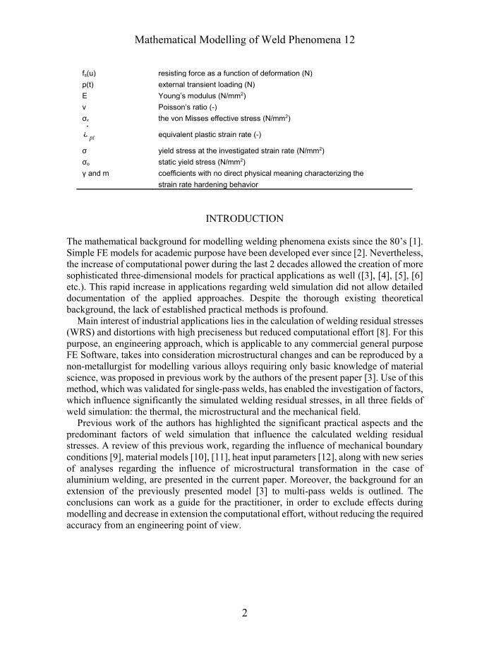
List of Notations

fr heat fraction deposited in the rear quadrant of Goldak’s heat

source (J)

ff heat fraction deposited in the front quadrant of Goldak’s heat

source (J)

Q thermal power or energy input rate (Watt or J/s)

C characteristic radius of flux distribution (m)

v welding source travel (m/s)

t time (s)

τ lag factor (“phase shift”) needed to define the position of weld heat

source source at time t = 0

V voltage (V)

I current of the weld metal arc (A)

η weld metal arc efficiency (-)

ρ density (Kg/m3)

c specific heat (J/(kg K))

T temperature (K)

Kxx, Kyy, Kzz thermal conductivity in the element’s x, y, and z directions (W/(m

K))

Q heat generation rate per unit volume (W/m3)

αse temperature dependent coefficient of thermal expansion

Tref reference temperature for thermal strains (°C)


2

fs(u) resisting force as a function of deformation (N)

p(t) external transient loading (N)

E Young’s modulus (N/mm2)

ν Poisson’s ratio (-)

σε the von Misses effective stress (N/mm2)

pl equivalent plastic strain rate (-)

σ yield stress at the investigated strain rate (N/mm2)

σο static yield stress (N/mm2)

γ and m coefficients with no direct physical meaning characterizing the

strain rate hardening behavior

INTRODUCTION

The mathematical background for modelling welding phenomena exists since the 80’s [1].

Simple FE models for academic purpose have been developed ever since [2]. Nevertheless,

the increase of computational power during the last 2 decades allowed the creation of more

sophisticated three-dimensional models for practical applications as well ([3], [4], [5], [6]

etc.). This rapid increase in applications regarding weld simulation did not allow detailed

documentation of the applied approaches. Despite the thorough existing theoretical

background, the lack of established practical methods is profound.

Main interest of industrial applications lies in the calculation of welding residual stresses

(WRS) and distortions with high preciseness but reduced computational effort [8]. For this

purpose, an engineering approach, which is applicable to any commercial general purpose

FE Software, takes into consideration microstructural changes and can be reproduced by a

non-metallurgist for modelling various alloys requiring only basic knowledge of material

science, was proposed in previous work by the authors of the present paper [3]. Use of this

method, which was validated for single-pass welds, has enabled the investigation of factors,

which influence significantly the simulated welding residual stresses, in all three fields of

weld simulation: the thermal, the microstructural and the mechanical field.

Previous work of the authors has highlighted the significant practical aspects and the

predominant factors of weld simulation that influence the calculated welding residual

stresses. A review of this previous work, regarding the influence of mechanical boundary

conditions [9], material models [10], [11], heat input parameters [12], along with new series

of analyses regarding the influence of microstructural transformation in the case of

aluminium welding, are presented in the current paper. Moreover, the background for an

extension of the previously presented model [3] to multi-pass welds is outlined. The

conclusions can work as a guide for the practitioner, in order to exclude effects during

modelling and decrease in extension the computational effort, without reducing the required

accuracy from an engineering point of view.


3

THEORETICAL BACKGROUND

MODELLING OF WELDING RESIDUAL STRESSES AND DISTORTION

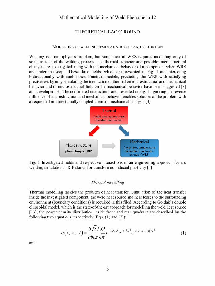
Welding is a multiphysics problem, but simulation of WRS requires modelling only of

some aspects of the welding process. The thermal behavior and possible microstructural

changes are investigated along with the mechanical behavior of a component when WRS

are under the scope. These three fields, which are presented in Fig. 1 are interacting

bidirectionally with each other. Practical models, predicting the WRS with satisfying

preciseness by only simulating the interaction of thermal on microstructural and mechanical

behavior and of microstructural field on the mechanical behavior have been suggested [8]

and developed [3]. The considered interactions are presented in Fig. 1. Ignoring the reverse

influence of microstructural and mechanical behavior enables solution of the problem with

a sequential unidirectionally coupled thermal–mechanical analysis [3].

Fig. 1 Investigated fields and respective interactions in an engineering approach for arc

welding simulation, TRIP stands for transformed induced plasticity [3]

Thermal modelling

Thermal modelling tackles the problem of heat transfer. Simulation of the heat transfer

inside the investigated component, the weld heat source and heat losses to the surrounding

environment (boundary conditions) is required in this filed. According to Goldak’s double

ellipsoidal model, which is the state-of-the-art approach for modelling the weld heat source

[13], the power density distribution inside front and rear quadrant are described by the

following two equations respectively (Eqn. (1) and (2)):

( )2 2 2 2 2 23 / 3 / 3[ ( )] /

6 3, , ,

f x a y b z v t cf Q

q x y z t e e eabc

− − − + −= (1)

and


4

( )2 2 2 2 2 23 / 3 / 3[ ( )] /6 3

, , , x a y b z v t crf Qq x y z t e e e

abc

− − − + −= . (2)

The effective energy input rate (thermal power, equal to the electric power of the arc

minus the losses) is predicted according to the following Eqn. (3) [3]

Q VI= . (3)

Heat input h is calculated by dividing Eqn. (3) with the welding speed. Proposed values

for the η coefficient for various weld types are proposed in [14]. Nevertheless, different

values usually in a range of ±10 % for same welding types are found elsewhere (see [2]

etc.). Combining the first thermodynamics law (conservation of energy) with Fourier’s law

for heat conduction and neglecting the fluid flow in the weld pool, the transient heat transfer

Eqn. (4) which governs the heat transfer inside the component is calculated [15]:

G

T T T Tc Q Kx Ky Kz

t x x y y z z

= + + +

. (4)

Heat losses are modelled according to Newton’s law of cooling (Eqn. (5))

( )f s b

qh T T

A= − . (5)

A transient thermal analysis is carried out, whereby the temperature history of the nodes

of the FE model are saved at each solution step.

Microstructural modelling

Various models have been proposed in the past, in order to predict the metallurgical

transformations during a weld thermal cycle ([16], [17] etc.). A straightforward engineering

approach, which was proposed by the authors of the present study [3], provided results with

sufficient preciseness. The method is applicable for the simulation of various materials [9],

[12], [10]. Main feature of the approach lies on the assignment of material models to the

finite elements inside the fusion zone (FZ) and the heat-affected zone (HAZ) during cooling

down based on predominant parameters of the thermal cycle, in order to simulate the

modified mechanical behavior of the transformed microstructure. The considered

parameters are the the maximum reached temperature inside a thermal cycle Tmax, the time

needed for the temperature to drop from 800 °C to 500 °C during cooling down inside a

thermal cycle t85, and the austenitization time ta, during which the temperature is above the

austenitization temperature (Ac1) inside a thermal cycle.

In the case of single-pass butt-welds the austinetization time is similar in all areas around the weld [2], [3]. Austinetization time influences the proportion of the parent material,

which is transformed to austenite during warm up and is subsequent to metallurgical

transformations during cooling down. This proportion is as well influenced by the


5

maximum achieved temperature. The coupled influence of these two parameters on the

proportion of the austenitized temperature, can be expressed only by the Tmax, if the

retardation effect is taken into consideration. When high heating rates and thus, short

austenitization times, are present the temperature at which full austenitization is achieved

(Ac3) is higher than the respective theoretically predicted value (for “static” slow warm

up). This effect was firstly mentioned by Leblond [16] and was integrated to the weld

modelling approach by the authors of the present paper [3] based on measurements of

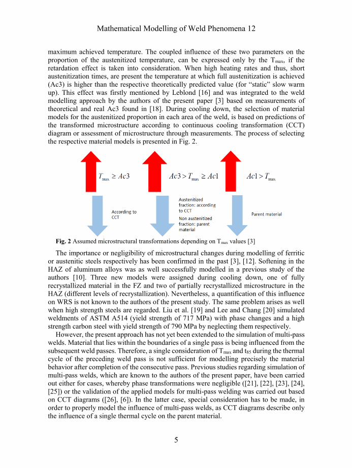
theoretical and real Ac3 found in [18]. During cooling down, the selection of material

models for the austenitized proportion in each area of the weld, is based on predictions of

the transformed microstructure according to continuous cooling transformation (CCT)

diagram or assessment of microstructure through measurements. The process of selecting

the respective material models is presented in Fig. 2.

Fig. 2 Assumed microstructural transformations depending on Tmax values [3]

The importance or negligibility of microstructural changes during modelling of ferritic

or austenitic steels respectively has been confirmed in the past [3], [12]. Softening in the

HAZ of aluminum alloys was as well successfully modelled in a previous study of the

authors [10]. Three new models were assigned during cooling down, one of fully

recrystallized material in the FZ and two of partially recrystallized microstructure in the

HAZ (different levels of recrystallization). Nevertheless, a quantification of this influence

on WRS is not known to the authors of the present study. The same problem arises as well

when high strength steels are regarded. Liu et al. [19] and Lee and Chang [20] simulated

weldments οf ASTM A514 (yield strength of 717 MPa) with phase changes and a high

strength carbon steel with yield strength of 790 MPa by neglecting them respectively.

However, the present approach has not yet been extended to the simulation of multi-pass

welds. Material that lies within the boundaries of a single pass is being influenced from the

subsequent weld passes. Therefore, a single consideration of Tmax and t85 during the thermal

cycle of the preceding weld pass is not sufficient for modelling precisely the material

behavior after completion of the consecutive pass. Previous studies regarding simulation of

multi-pass welds, which are known to the authors of the present paper, have been carried

out either for cases, whereby phase transformations were negligible ([21], [22], [23], [24],

[25]) or the validation of the applied models for multi-pass welding was carried out based on CCT diagrams ([26], [6]). In the latter case, special consideration has to be made, in

order to properly model the influence of multi-pass welds, as CCT diagrams describe only

the influence of a single thermal cycle on the parent material.


6

Modelling of mechanical behaviour

During modelling of the mechanical field, the nodal temperature history from the prior

transient thermal analysis is applied as body force nodal loads (thermal strains εth), which

are calculated based on the temperature dependent coefficient of thermal expansion αse [15]

( ) ( )th se

refa T T T = − . (6)

Solution takes place in a quasi-static structural analysis, whereby temperature dependent

material parameters and the restraints applied to the real welded component are modelled

[3]. Quasi-static structural analysis is governed by the following equation:

( ) ( ) 0sf u p t− = . (7)

Usually, components are clamped down during welding. Fixing of the respective nodes

in the FE models is a common approach of modelling but deviates from physical restraining

reality. An alternative approach applied elsewhere [9] is the use of linear spring elements,

restraining the respective nodes (see Fig. 4). The free edge of the spring is then fixed parallel

to its length direction. Therewith, only very small displacements are allowed, which

coincides with the situation in real “clamping”.

In most cases, mechanical solution is based on classical theory of strain-rate independent

plasticity [27]. Total mechanical strain is decomposed to elastic and plastic parts (Eqn. (8)).

mech

tot el pl = +

. (8)

The stress σ is proportional to the elastic strain εel according to Hooke’s law for linear

isotropic material behaviour, which is presented in terms of Young’s modulus and

Poisson’s ratio and in index notation in the following equation (Eqn. (9)),

1( ( )),ij ij kk ij ijv

E = − −

(9)

where δij is the Kronecker delta. Von Mises yield criterion (Eqn. (10)

( , ) 0,y e yf = − =

(10)

is widely applied for metallic materials, where σε is the von Misses effective stress

23 1: ( )

2 3e s tr

= −

. (11)


7

Isotropic hardening is usually applied, during welding simulations, as theoretically,

heating the material up to near melting temperature erases previous hardening history and

the material deforms as virgin [23], [28]. Nevertheless, kinematic hardening provided better

results elsewhere [9], [12]. In some cases, even mixed hardening models are proposed [28].

Lindgren [8] proposed that during weld simulation, when very high accuracy is required,

strain-rate dependent plasticity should be considered, without providing though any

information regarding the order of magnitude of the influence on calculated WRS. Previous

analyses of the authors of the present paper have showed that in the heat affected zone

(HAZ) and the fusion zone (FZ) of a 3-pass butt-weld, strain rates of up to 0.122 s-1 are

present [11]. Although this value lies clearly lower than the classical dynamic cases such

as modelling of ballistic tests or car crash simulation (100 s-1), still clearly deviates from

the static case ( 0 → ). Several models have been proposed in the past for modelling of

the strain-rate dependent behavior of steel. The following model proposed by Perzyna in

1966 [29] is appropriate for implicit FE simulations like in the present case (Eqn. 12)

. (12)

REVIEWING THE INLUEFNCE OF INPUT PARAMETERS

Results from previous and new FE analyses, which were all carried out according to the

above-described theoretical background, are presented in the current study in order to

review specific aspects of weld simulation. FE commercial software ANSYS [15] was

applied in all cases. Solid 8 node elements “solid 90” and “solid 180” were applied for the

transient thermal and the static structural analyses respectively in all cases. Mesh element

dimensions were 0.4 mm x 0.4 mm x 5 mm (width x height x length) in the FZ and the

HAZ in all cases. The following aspects were investigated:

A: MODELLING OF MECHANICAL BOUNDARY CONDITIONS (BC)

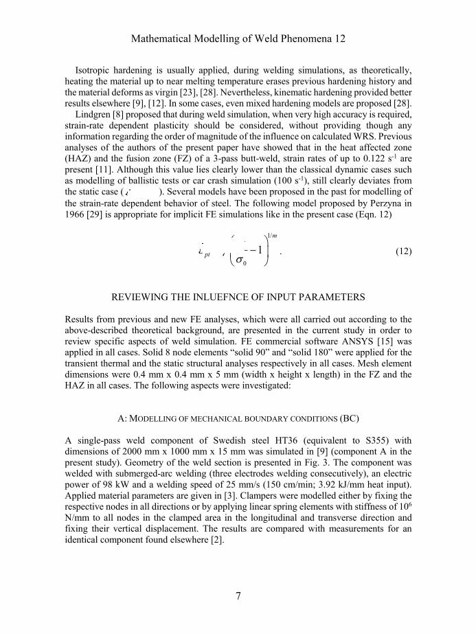
A single-pass weld component of Swedish steel HT36 (equivalent to S355) with

dimensions of 2000 mm x 1000 mm x 15 mm was simulated in [9] (component A in the

present study). Geometry of the weld section is presented in Fig. 3. The component was

welded with submerged-arc welding (three electrodes welding consecutively), an electric

power of 98 kW and a welding speed of 25 mm/s (150 cm/min; 3.92 kJ/mm heat input).

Applied material parameters are given in [3]. Clampers were modelled either by fixing the

respective nodes in all directions or by applying linear spring elements with stiffness of 106

N/mm to all nodes in the clamped area in the longitudinal and transverse direction and

fixing their vertical displacement. The results are compared with measurements for an

identical component found elsewhere [2].

1/

0

1

m

pl

= −


8

Fig. 3 Investigated component A

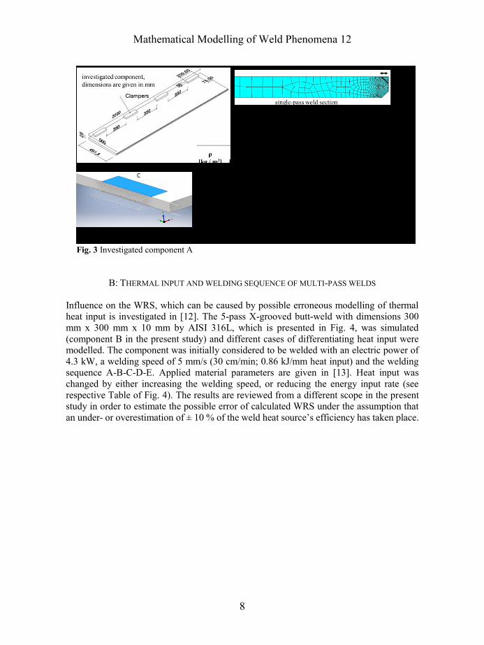
B: THERMAL INPUT AND WELDING SEQUENCE OF MULTI-PASS WELDS

Influence on the WRS, which can be caused by possible erroneous modelling of thermal

heat input is investigated in [12]. The 5-pass X-grooved butt-weld with dimensions 300

mm x 300 mm x 10 mm by AISI 316L, which is presented in Fig. 4, was simulated

(component B in the present study) and different cases of differentiating heat input were

modelled. The component was initially considered to be welded with an electric power of

4.3 kW, a welding speed of 5 mm/s (30 cm/min; 0.86 kJ/mm heat input) and the welding

sequence A-B-C-D-E. Applied material parameters are given in [13]. Heat input was

changed by either increasing the welding speed, or reducing the energy input rate (see

respective Table of Fig. 4). The results are reviewed from a different scope in the present

study in order to estimate the possible error of calculated WRS under the assumption that

an under- or overestimation of ± 10 % of the weld heat source’s efficiency has taken place.


9

Fig. 4 Investigated component B

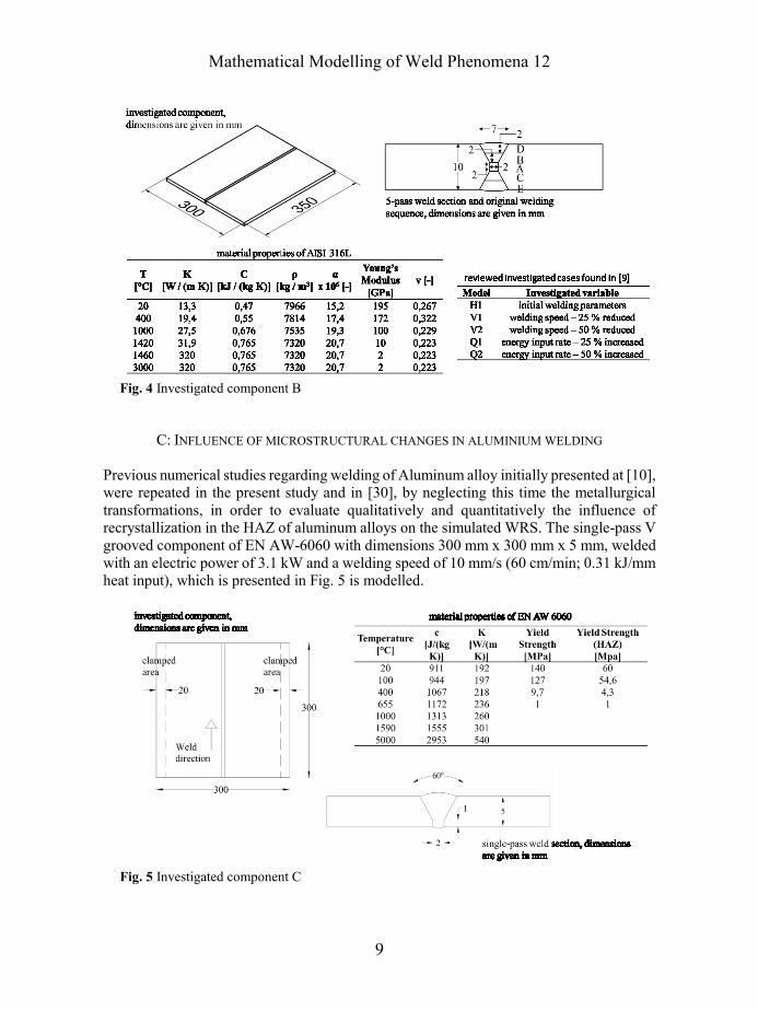
C: INFLUENCE OF MICROSTRUCTURAL CHANGES IN ALUMINIUM WELDING

Previous numerical studies regarding welding of Aluminum alloy initially presented at [10],

were repeated in the present study and in [30], by neglecting this time the metallurgical

transformations, in order to evaluate qualitatively and quantitatively the influence of

recrystallization in the HAZ of aluminum alloys on the simulated WRS. The single-pass V

grooved component of EN AW-6060 with dimensions 300 mm x 300 mm x 5 mm, welded

with an electric power of 3.1 kW and a welding speed of 10 mm/s (60 cm/min; 0.31 kJ/mm

heat input), which is presented in Fig. 5 is modelled.

Fig. 5 Investigated component C


10

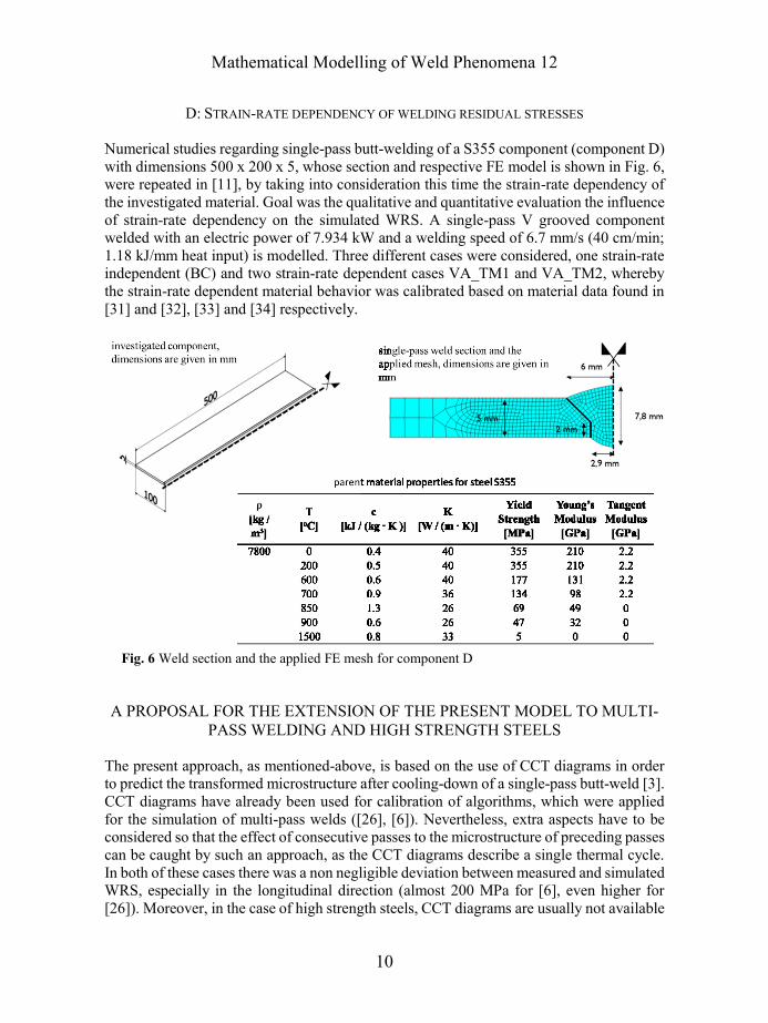
D: STRAIN-RATE DEPENDENCY OF WELDING RESIDUAL STRESSES

Numerical studies regarding single-pass butt-welding of a S355 component (component D)

with dimensions 500 x 200 x 5, whose section and respective FE model is shown in Fig. 6,

were repeated in [11], by taking into consideration this time the strain-rate dependency of

the investigated material. Goal was the qualitative and quantitative evaluation the influence

of strain-rate dependency on the simulated WRS. A single-pass V grooved component

welded with an electric power of 7.934 kW and a welding speed of 6.7 mm/s (40 cm/min;

1.18 kJ/mm heat input) is modelled. Three different cases were considered, one strain-rate

independent (BC) and two strain-rate dependent cases VA_TM1 and VA_TM2, whereby

the strain-rate dependent material behavior was calibrated based on material data found in

[31] and [32], [33] and [34] respectively.

Fig. 6 Weld section and the applied FE mesh for component D

A PROPOSAL FOR THE EXTENSION OF THE PRESENT MODEL TO MULTI-

PASS WELDING AND HIGH STRENGTH STEELS

The present approach, as mentioned-above, is based on the use of CCT diagrams in order

to predict the transformed microstructure after cooling-down of a single-pass butt-weld [3].

CCT diagrams have already been used for calibration of algorithms, which were applied

for the simulation of multi-pass welds ([26], [6]). Nevertheless, extra aspects have to be

considered so that the effect of consecutive passes to the microstructure of preceding passes

can be caught by such an approach, as the CCT diagrams describe a single thermal cycle.

In both of these cases there was a non negligible deviation between measured and simulated

WRS, especially in the longitudinal direction (almost 200 MPa for [6], even higher for

[26]). Moreover, in the case of high strength steels, CCT diagrams are usually not available


11

in literature although the research interest on these materials is increasing in the last years

(see [35]).

With the present approach, in the case, whereby a CCT diagram is available, it can be

assumed that succeeding weld passes carry on the austenitization of the boundary areas of

previous passes, if there was no full austenitization, or that there is a reaustenitization of

the previously fully-austenitized materials. In both cases it can be assumed as well that the

investigated material’s cooling down behaviour still can be described by the CCT diagram

of the parent material despite the thermal treatment of the preceding passes.

An alternative approach would be the use of hardness measurements on the macro

sections of welded components. This measurements could be applied either as a validation

of the modelling approach based on the CCT diagrams validating the above-mentioned

assignments or as direct input for the material behaviour of various areas of the weld

section. The relation of hardness and yield strength of steel has been proven in several cases

in the past and various equations have been proposed such as in [36] and [37]. Moreover,

the hardness of the individual steel phases at room temperature as a function of the chemical

composition can be analytically calculated [38]. Knowing the proportion of the

metallurgical phases and the yield strength and hardness, it could be possible to calculate

the proportion of phases at each area of the macro section based on the hardness

measurements.

RESULTS AND DISCUSSION

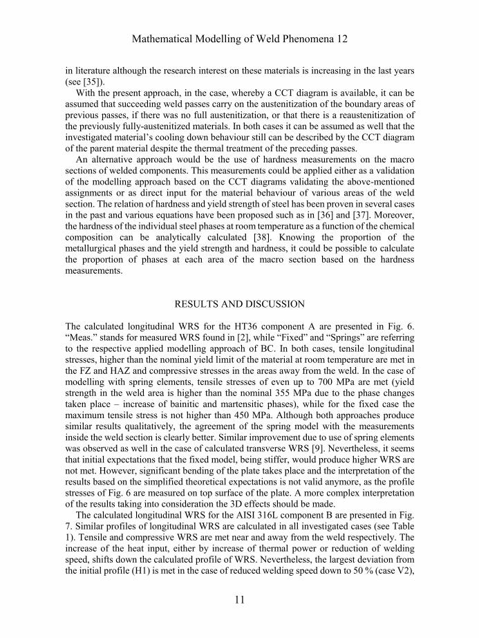
The calculated longitudinal WRS for the HT36 component A are presented in Fig. 6.

“Meas.” stands for measured WRS found in [2], while “Fixed” and “Springs” are referring

to the respective applied modelling approach of BC. In both cases, tensile longitudinal

stresses, higher than the nominal yield limit of the material at room temperature are met in

the FZ and HAZ and compressive stresses in the areas away from the weld. In the case of

modelling with spring elements, tensile stresses of even up to 700 MPa are met (yield

strength in the weld area is higher than the nominal 355 MPa due to the phase changes

taken place – increase of bainitic and martensitic phases), while for the fixed case the

maximum tensile stress is not higher than 450 MPa. Although both approaches produce

similar results qualitatively, the agreement of the spring model with the measurements

inside the weld section is clearly better. Similar improvement due to use of spring elements

was observed as well in the case of calculated transverse WRS [9]. Nevertheless, it seems

that initial expectations that the fixed model, being stiffer, would produce higher WRS are

not met. However, significant bending of the plate takes place and the interpretation of the

results based on the simplified theoretical expectations is not valid anymore, as the profile

stresses of Fig. 6 are measured on top surface of the plate. A more complex interpretation

of the results taking into consideration the 3D effects should be made.

The calculated longitudinal WRS for the AISI 316L component B are presented in Fig.

7. Similar profiles of longitudinal WRS are calculated in all investigated cases (see Table

1). Tensile and compressive WRS are met near and away from the weld respectively. The

increase of the heat input, either by increase of thermal power or reduction of welding

speed, shifts down the calculated profile of WRS. Nevertheless, the largest deviation from

the initial profile (H1) is met in the case of reduced welding speed down to 50 % (case V2),


12

which equals to an increase of heat input up to 100%. A difference of up to 150 MPa or 28

% between the peak tensile stresses of those two cases is observed. Similar but not so

significant differentiation of the transverse WRS profiles was observed as well [13].

Fig. 7 Longitudinal WRS – left: Component A (HT36) – right: Component B (316L),

resulting WRS on the top of the component, for the investigated cases presented in Table 1

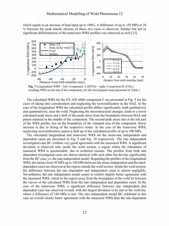
The calculated WRS for the EN AW 6060 component C are presented in Fig. 5 for the

cases of taking into consideration and neglecting the recrystallization in the HAZ. In the

case of the longitudinal WRS the calculated profile differs significantly, both qualitatively

and quantitatively, near the weld. Neglecting the microstructural changes, leads to a lower

calculated peak stress and a shift of this peak stress from the boundaries between HAZ and

parent material in the middle of the component. The second peak stress met at the left part

of the WRS profile, lies on the boundaries of the clamped area of the component. Stress

increase is due to fixing of the respective nodes. In the case of the transverse WRS,

neglecting recrystallization causes a shift up of the calculated profile of up to 100 MPa.

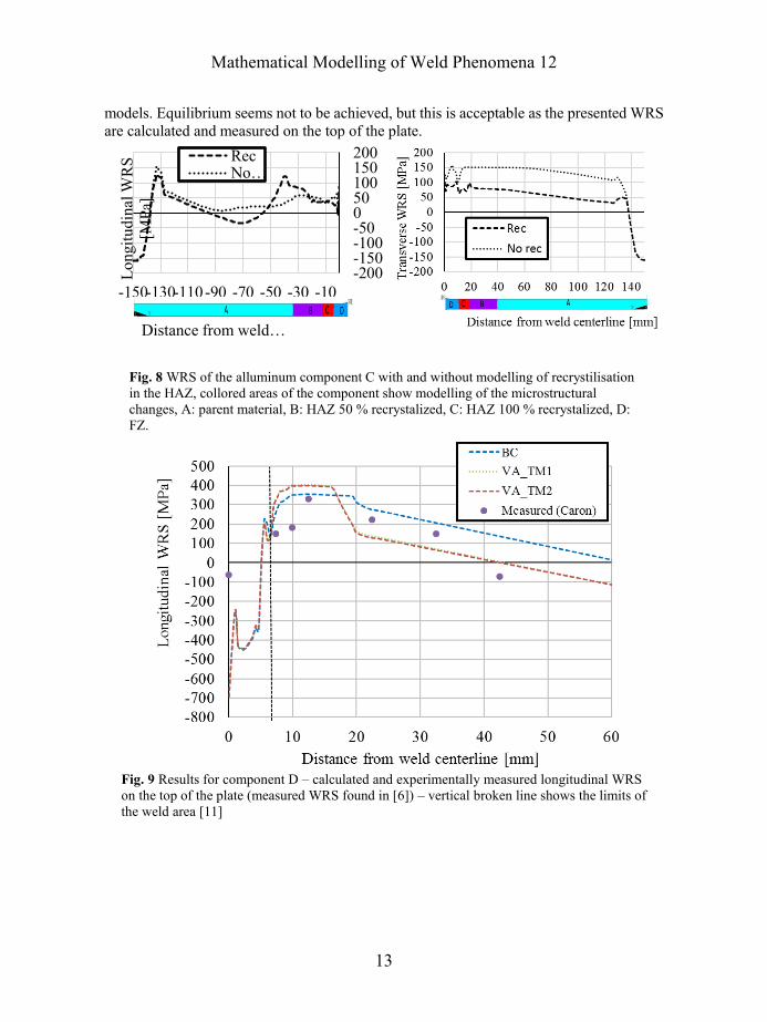
The calculated longitudinal and transverse WRS for the strain-rate independent and

dependent cases are presented in Fig. 9 and Fig. 10 respectively. The rate independent

investigated case BC exhibits very good agreement with the measured WRS. A significant

deviation is observed only inside the weld section, a region where the robustness of

measured WRS is questionable, due to technical reasons. The profiles from both rate

dependent investigated cases are almost identical with each other but deviate significantly

from the BC case, i.e. the rate-independent model. Regarding the profiles of the longitudinal

WRS, deviations from 50 MPa up to 100 MPa between the strain-independent and the rated-

dependent cases are observed at the region outside the weld section. Inside the weld section,

the difference between the rate dependent and independent cases is almost negligible.

Nevertheless, the rate independent model seems to exhibit slightly better agreement with

the measured WRS, which in the region away from the boundaries of the weld lie between

the curves of the calculated WRS from the rate independent and dependent cases. In the

case of the transverse WRS, a significant difference between rate independent and

dependent case was observed overall, with the largest deviation to be met at the weld toe, where a difference of 140 MPa is met. The rate independent model BC exhibited in this

case an overall clearly better agreement with the measured WRS than the rate-dependent


13

models. Equilibrium seems not to be achieved, but this is acceptable as the presented WRS

are calculated and measured on the top of the plate.

Fig. 8 WRS of the alluminum component C with and without modelling of recrystilisation

in the HAZ, collored areas of the component show modelling of the microstructural

changes, A: parent material, B: HAZ 50 % recrystalized, C: HAZ 100 % recrystalized, D:

FZ.

Fig. 9 Results for component D – calculated and experimentally measured longitudinal WRS

on the top of the plate (measured WRS found in [6]) – vertical broken line shows the limits of

the weld area [11]

-200-150-100-50050100150200

-150-130-110-90 -70 -50 -30 -10

Lo

ngit

udin

al W

RS

[MP

a]

Distance from weld …

RecNo…


14

Fig. 10 Results for component D – calculated and experimentally measured transverse WRS on

the top of the plate (measured WRS found in [6]) – vertical broken line shows the limits of the

weld area [11]

CONCLUSIONS AND FUTURE WORK

The following conclusions were drawn, based on the above-presented results:

Applied approach for modelling of clampers during a weld simulation can have a

significant effect on the calculated WRS, at least in the case of butt-welds. The use of spring

elements for modelling the longitudinal and transverse restraints in the clamped area

produces results that show better agreement with experimentally measured WRS.

Moreover, as higher tensile WRS are calculated, this approach lies on the safe side. This

modelling approach is therefore suggested for adoption in practical applications as well.

A possible erroneous modelling of the weld heat source could lead to an underestimation

of the WRS and therefore non-conservative results. An increase of 100 % of the heat input

led to a reduction of 28 % of the peak tensile stress (worst case scenario). Assuming a linear

behavior, an overestimation of 10 % of the heat source coefficient would lead to an

underestimation of 2.8 % of the peak tensile stresses. This deviation lies in the boundaries

of the acceptable numerical error, of practical weld simulations (± 10 % [3]). Therefore,

applying values for the weld metal arc efficiency from literature or previous measurements

during the simulation of WRS, is considered valid.

Aluminum welding simulations neglecting the recrystallization in the HAZ, produce

erroneous results. A lower longitudinal peak stress is calculated and is present at the middle

of the component. Simulations considering the microstructural changes show that the peak

stress is met on the boundaries of the HAZ, exhibiting a much more crucial case, regarding

fatigue strength of the investigated component. Therefore, neglecting recrystallization in


15

the HAZ of aluminum weld during weld simulation is not conservative and should be

avoided.

Applying strain rate dependent material models during a weld simulation produces

significant deviation in the profiles of calculated WRS in comparison with the classical

static material models. A deviation of up to 150 MPa was observed in the present case

between rate independent and dependent cases. Therefore, strain rate dependency cannot

be neglected during weld simulation when high accuracy is required. Nevertheless, the

strain-rate independent case provided results with better agreement in the case of transverse

WRS and this incompatibility has to be clarified.

The present method has been proven to provide accurate results with less computational

effort and increased simplicity in comparison with previous modeling approaches for single

pass-welds [3]. A validation of the above-mentioned extension for the case of multi-pass

welds and high strength steels is therefore dictated. Comparison with measured WRS of

real multi-pass welds has to be carried out and the effectiveness should be compared with

other approaches [26], [6].

ACKNOWLEDGEMENTS

The above presented work was carried out as a part of the framework of [39].

REFERENCES

[1] J. H. ARGYRIS, J. SJIMMAT AND K. J. WILLAM: ‘Computational Aspects of Welding Stress

Analysis’, Computer Methods in Applied Mechanics and Engineering, Vol. 33, No. 1-3, pp.

635-665, 1982.

[2] B. ANDERSSON: ‘Thermal Stresses in a Submerged-Arc Welded Joint Considering Phase

Transformations’, Trans. ASME, Vol. 100, pp. 356-362, 1978.

[3] P. KNOEDEL, S. GKATZOGIANNIS AND T. UMMENHOFER: ‘Practical Aspects of Welding

Residual Stress Simulation’, Journal of Constructional Steel Research, Vol. 132, pp. 83-96,

2017.

[4] P. DONG: ‘Residual Stress Analyses of a Multi-Pass Girth Weld: 3-D Special Shell Versus

Axisymmetric Models’, Journal of Pressure Vessel Technology, Vol. 123, No. 2, pp. 207-213,

2001.

[5] D. DENG AND H. MURAKAWA: ‘Numerical simulation of temperature field and residual stress

in multi-pass welds in stainless steel pipe and comparison with experimental measurements’,

Computational Materials Science, Vol. 37, pp. 269-277, 2006.

[6] C. HEINZE, C. SCHWENK, M. RETHMEIER AND J. CARON: ‘Numerical Sensitivity Analysis of

Welding-Induced Residual Stress Depending on Variations in Continuous Cooling

Transformation Behavior’, Front. Mater. Sci., Vol. 5, No. 2, pp. 168-178, 2011.

[7] A. A. BHATTI, Z. BARSOUM, H. MURAKAWA AND I. BARSOUM: ‘Influence of Thermo-

Mechanical Material Properties of Different Steel Grades on Welding Residual Stresses and

Angular Distortion’, Materials and Design, Vol. 65, pp. 878-889, 2015.

[8] L. E. LINDGREN: Computational Welding Mechanics – Thermomechanical and Microstructural

Simulations, 1st Edition, Woodhead Publishing, Cambridge, England, 2007.

[9] S. GKATZOGIANNIS, P. KNOEDEL AND T. UMMENHOFER: ‘FE Welding Residual Stress

Simulation – Influence of Boundary Conditions and Material Models’, EUROSTEEL 2017,

September 13–15, 2017, Copenhagen, Denmark, Ernst & Sohn, CE/papers, 2017.


16

[10] P. KNOEDEL, S. GKATZOGIANNIS AND T. UMMENHOFER: ‘FE Simulation of Residual Welding

Stresses: Aluminum and Steel Structural Components’, Key Engineering Materials, Vol. 710,

pp. 268-274, 2016.

[11] S. GKATZOGIANNIS, P. KNOEDEL AND T. UMMENHOFER: ‘Strain-Rate Dependency of Simulated

Welding Residual Stresses’, Journal of Material Performance and Engineering, 2017.

[12] S. GKATZOGIANNIS, P. KNOEDEL AND T. UMMENHOFER: ‘Influence of Welding Parameters on

the Welding Residual Stresses’, Proceedings of the VII International Conference on Coupled

Problems in Science and Engineering, Rhodes Island, Greece, June 12 – 14, pp. 767-778, 2017.

[13] J. A. GOLDAK, A. CHAKRAVARTI AND M. BIBBY: ‘A New Finite Element Model for Welding

Heat Sources’, Metall. Trans. B, Vol. 15, pp. 299-305, 1984.

[14] J. N. DUPONT AND A. R. MARDER: ‘Thermal Efficiency of Arc Welding Processes’, Weld. J.,

pp. 406-416, 1995.

[15] ANSYS® Academic Research, Release 18.2, Help System, ANSYS, Inc., 2018.

[16] J. B. LEBLOND AND J. DEVAUX: ‘A New Kinetic Model for Anisothermal Metallurgical

Transformations in Steels including Effect of Austenite Grain Size’, ACTA Metall., Vol. 32,

pp. 137-146, 1984.

[17] D. P. KOISTINEN AND R. E. MARBURGER: ‘A General Equation Prescribing the Extent of the

Austenite-Martensite’, ACTA Metall., Vol. 7, pp. 59-61, 1959.

[18] M. Q. MACEDO, A. B. COTA AND F. G. DA S. ARAÚJO: ‘The Kinetics of Austenite Formation at

High Heating Rates’, Metal. E Mater., Vol. 64, pp. 163-167, 2011.

[19] W. LIU, J. MA, F. KONG, S. LIU AND R. KOVACEVIC: ‘Numerical Modeling and Experimental

Verification of Residual Stress in Autogenous Laser Welding of High-Strength Steel’, Lasers

Manuf. Mater. Process. 2, pp. 24-42, 2015.

[20] C. H. LEE AND K .H. CHANG: ‘Prediction of Residual Stresses in High Strength Carbon Steel

Pipe Weld Considering Solid-State Phase Transformation Effects’, Computers and Structures,

Vol. 89, pp. 256-265, 2015.

[21] B. BRICKSTAD AND B. L. JOSEFSON: ‘A Parametric Study of Residual Stresses in Multi-Pass

Butt-Welded Stainless Steel Pipes’, International Journal of Pressure Vessels and Piping, Vol.

75, pp. 11-25, 1998.

[22] D. E. KATSAREAS, C. OHMS AND A. G. YOUTSOS: ‘Finite Element Simulation of Welding in

Pipes: A Sensitivity Analysis’, Proceedings of a Special Symposium held within the 16th

European Conference of Fracture - ECF16, Alexandroupolis, Greece, 3-7 July, 2006, pp. 15-

26, 2006.

[23] H. WOHLFAHRT, T. NITSCHKE-PAGEL, K. DILGER, D. SIEGELE, M. BRAND, J. SAKKIETTIBUTRA

AND T. LOOSE: ‘Residual Stress Calculations and Measurements - Review and Assessment of

the IIR Round Robin Results’, Welding in the World, Vol. 56, pp. 120-140, 2012.

[24] S. NAKHODOCHI, A. SHOKUFAR, S. A. IRAJ AND B. G. THOMAS: ‘Residual Stress Calculations

and Measurments- Review and Assessment of the IIR Round Robin Results’, Journal of

Pressure Vessel Technology, Vol. 137, 2015.

[25] C. K. LEE, S. P. CHIEW AND J. JIANG: ‘3D Residual Stress Modelling of Welded High Strength

Steel Plate-to-Plate Joints’, Journal of Constructional Steel Research, Vol. 84, pp. 94-104,

2013.

[26] L. BÖRJESSON AND L. E. LINDGREN: ‘Simulation of Multipass Welding With Simultaneous

Computation of Material Properties’, Journal of Engineering Materials and Technology, Vol.

123, pp. 106-111, 2001.

[27] J. LUBLINER: ‘Plasticity Theory’, Dover Publications, 3d Edition, New York, USA, 2008.

[28] J. MULLINS AND J. GUNNARS: ‘Influence of Hardening Model on Weld Residual Stress

Distribution’, Research Report 2009:16, Inspecta Technology AB, Stockholm, Sweden, 2009.


17

[29] P. PERZYNA: ‘Fundamental Problems in Viscoplasticity’, Advances in Applied Mechanics, Vol.

5, pp. 243-377, 1966.

[30] S. GKATZOGIANNIS, P. KNOEDEL AND T. UMMENHOFER: ‘Reviewing the Influence of Welding

Setup on FE-simulated Welding Residual Stresses’, Proceedings of the 10th European

Conference on Residual Stresses - ECRS10, Leuven, Belgium, on 11-14 September, 2018.,

accepted for publication.

[31] N. JONES: Structural Impact, 2nd Edition, Cambridge University Press, New York, USA, 2012.

[32] D. FORNI, B. CHIAIA AND E. CADONI: ‘Strain Rate Behaviour in Tension of S355 Steel: Base

for progressive collapse analysis’, Engineering Strcutrures, Vol. 119, pp. 167-173, 2016.

[33] M. KNOBLOCH, J. PAULI, M. FONTANA: ‘Influence of The Strain Rate on the Mechanical

Properties of Mild Carbon Steel at Elevated Temperatures’, Materials and Design, Vol. 49, pp.

553-565, 2013.

[34] D. FORNI, B. CHIAIA AND E. CADONI: ‘High Strain Rate Response of S355 at High

Temperatures’, Materials and Design, Vol. 94, pp. 467-478, 2016.

[35] J. SCHUBNEL, S. GKATZOGIANNIS, M. FARAJIAN, P. KNOEDEL, T. LUKE AND T. UMMENHOFER:

‘Rechnergestütztes Bewertungstool zum Nachweis der Lebensdauerverlängerung von mit dem

Hochfrequenz-Hämmerverfahren (HFMI) behandelten Schweißverbindungen aus hochfesten

Stählen’, Research Project DVS 09069 – IGF 19227 N, 2018 (in progress).

[36] E. J. PAVLINA AND C.J. VAN TYNE: ‘Correlation of Yield Strength and Tensile Strength with

Hardness for Steels’, Journal of Materials Engineering and Performance, Vol. 17, No. 6, pp.

888-893, 2008.

[37] P. ZHANG, S. X. LI AND Z. F. ZHANG: ‘General Relationship Between Strength and Hardness’,

Materials Science and Engineering A, Vol. 529, No. 6, pp. 62-73, 2011.

[38] J. HILDEBRAND: ‘Numerische Schweißsimulation: Bestimmung von Temperatur, Gefüge und

Eigenspannung an Schweißverbindungen aus Stahl- und Glaswerkstoffen‘, Dissertation,

Bauhaus-Universität Weimar, 2008.

[39] S. GKATZOGIANNIS: ‘Finite Element Simulation of High Frequency Hammer Peening’,

Doctoral Thesis , KIT, Karlsruhe Institute of Technology, 2018 (in progress).

Documents

SIMULATION OF WELDING RESIDUAL STRESSES FROM THEORY …