SIMULATION OF IBM 3494 AUTOMATED TAPE LIBRARY …media.aero.und.edu/cs.und.edu/documents/ShantiSwarupa.pdf · SIMULATION OF IBM 3494 AUTOMATED TAPE LIBRARY ... Level 0 Data Flow Diagram

SIMULATION OF IBM 3494 AUTOMATED TAPE LIBRARY

AND TAPE ROBOT, IN CSIM 17

by

Shanti Pinreddy Swarupa Bachelor of Technology, Kakatiya Institute of Technology and Sciences, 1995

Master of science, university of North Dakota, 2000

A project

Submitted to the Graduate Faculty

of the

University of North Dakota

in partial fulfillment of the requirements

for the degree of

Master of Science

Grand Forks, North Dakota December 2002

iii

TABLE OF CONTENTS

LIST OF FIGURES .............................................................................................................v LIST OF TABLES .............................................................................................................. vi ACKNOWLEDGEMENTS ............................................................................................... vii ABSTRACT.......................................................................................................................viii CHAPTER

I INTRODUCTION................................................................................................1

1.1 Problem Statement .................................................................................1

1.2.Requirements .........................................................................................2

1.3 Structure of This Report.........................................................................3

II SCOPE OF THE PROJECT, HPSS, ARM, 3494 TAPE LIBRARY...............4

2.1 Scope......................................................................................................4

2.2 Overview of HPSS storage servers with respect to ARM .....................6

2.3 ARM (Atmospheric Radiation Measurement ........................................8

2.3.1 ARM archive usage Statistics useful for the model..............10

2.4 Details of tape libraries IBM 3494 Magstar Tape Library...................12

III SOFTWARE ENGINEERING TECHNIQUES, DESIGN AND

IMPLEMENTATION................................................................................18

3.1 Project Process ....................................................................................18

3.1.1 Incremental Design ...............................................................18

3.2 System Engineering Models ...............................................................21

3.2.1 Data Flow Diagrams (DFD)..................................................22

3.3 Implementation ...................................................................................24

3.4 Verification and validation..................................................................37

IV EXPERIMENTAL DESIGN ...........................................................................38

4.1 Production Runs ..................................................................................38

V CONCLUSIONS AND FUTURE WORK ......................................................42

APPENDIX A........................................................................................................45

iv

USER MANUAL...................................................................................................46

APPENDIX B........................................................................................................49

IMPLEMENTATION CODE................................................................................50

REFERENCES ......................................................................................................55

v

LIST OF FIGURES

1. System Architecture supported by HPSS ........................................................................7

2. Measurements gathered by the ARM archive..................................................................9

3. Request statistics of the ARM archive for Get Requests ..............................................11

4. Request statistics of the ARM archive for Put Requests ...............................................12

5. The IBM 3494 Automated Tape Library. .....................................................................13

6. Control Flow Diagram ..................................................................................................20

7. Level 0 Data Flow Diagram...........................................................................................22

8. Level 1 Data Flow Diagram...........................................................................................23

9. The Implementation Model............................................................................................27

vi

LIST OF TABLES

1. Details of IBM 3494 Automated Tape Library..............................................................24

2. Results of Production Runs for experiments 1 and 2.....................................................40



vi

ACKNOWLEDGEMENTS I would like to thank my advisor, Dr.Thomas Wiggen for the great support and guidance

provided to me in every step of the project.

Thanks to my graduate director for the helpful tips provided for my project.

I would like to thank the staff of the department of Computer Science for their care and

help.

I would also like to thank the reviewers for the helpful comments.

Thanks to my parents for the love and support they have given me.

vii

ABSTRACT

Lately there has been great advancement in computational speed in high performance

computing. Relatively there is less improvement in I/O performance. Greater processing

speeds have created the need for faster and more efficient I/O as well as for the storage and

retrieval of vast amounts of data. Robotic Storage Libraries are most important components

of the mass storage devices, which aid in the efficient storage and retrieval of such huge

amounts of data. This paper presents results of a queuing model. The effects of interactive

Get, Put requests, migration of requests at the ARM (Atmospheric Radiation Measurement)

archive using the IBM 3494 Robotic Tape Libraries are studied with the intention of

predicting the factors to have better I/O performance. The model is experimented with

different configurations of drive allocations, tape sizes and data transfer rates. The results

predict that, with the increase in number of drives dedicated to the Get requests there is a

substantial improvement in response times of the Get drives along with a great reduction in

queue sizes. Increase in data transfer rates and tape sizes also provide better performance.

The final conclusions have been made keep cost as an important criterion. The model is

developed though the use of discrete event simulation, in CSIM17, to be embedded into a

developing model for HPSS (High Performance Storage System).

1

CHAPTER I

INTRODUCTION

1.1 problem statement

Scientific projects like the Earth Observing System (EOS), magnetic energy fusion

modeling and climate modeling, generate terabytes of data that must be archived and

made available for further processing and analysis. Data management systems designed

to manage data of this order of magnitude employ a storage hierarchy to provide

efficient and cost effective access to data. The hierarchical mass storage systems consist

of three layers of storage. The first (i.e. online storage) consists of magnetic disks, which

provide fast access time, but at a relatively high cost per byte. The second layer (i.e. near

line storage) utilizes robotic tape libraries (RTL), and the third layer (i.e. offline storage)

consists of freestanding tape libraries with human operators performing the mounting and

unmounting of tapes from the drives. The most common type of device used to form the

second layer of the storage hierarchy of mass storage systems is RTL, which is very

popular because it combines a very low cost/byte ratio with a relatively low average

access time. These complex storage systems must be configured to handle the flow of

data efficiently with which must faster I/O speeds. There are no simple mathematical

models to study such systems. My model analyses the performance of such systems using

IBM 3494 as the standard RTL and predicts the optimal requirements for faster I/O and

low cost.

2

1.2 Requirements

The outcome of the system engineering process is the specification of a computer-based

system or product at the different levels. It provides an appropriate way of understanding

the needs of the customer, analyzing need, assessing feasibility, finding a reasonable

solution, validating the specification and managing the requirements as they are

transformed into an operational system.

The work products of this phase are:

1. Statement of need.

2. Scope for the system.

3. List of customers.

4. Description of the system in technical environment.

5. Set of usage scenarios and prototypes.

The specification is the final work product produced by the system and requirements

engineers. It serves as the foundation for HW engineering, SW engineering and human

engineering. It describes the information (data and control) that is input to and output

from the system. Requirements validation examines the specification to ensure that the

system requirements have been stated unambiguously, inconsistencies, omissions, errors

have been detected and corrected and that the work products confirm to the standards.

1.Statement of need

This simulation model developed in CSIM analyses the performance of the IBM 3494

Tape Libraries for archiving and retrieving the ARM (Atmospheric Radiation

Measurement) data with the intention to configure and allocate I/O resources better.

2. Scope for the system.

3

The model considers the operation of the tape library only, but the interface to the outside

world is not modeled. Refer Section 2.1 for further details.

3. List of Customers.

There are no real customers for the model being developed at present. The model is

developed for the ARM (Atmospheric Radiation Measurement) data, Refer to Section

3.2.

4. Description of the System in technical environment.

Refer to Section 2.4 .

1.3 Structure of This Report

The problem and requirements are dealt in the first section of the report. Chapter II deals

with High Performance Storage System servers and the Atmospheric Radiation

Measurement program. Chapter III describes the Software Engineering principles that

were applied during development of this simulation model and the implementation steps.

Chapter IV describes the final model and verification and validation process. Chapter V

analyses the outputs of our production runs, draws conclusions and provides some ideas

for future work.

4

CHAPTER II

SCOPE OF THE PROJECT, HPSS, ARM, 3494 TAPE LIBRARY

2.1 Scope

The improvements in computational speeds have increased the gap between

processor and computational speed. The current storage systems can transfer only tens of

megabytes of data per second. As a result scientists have to spend hours to retrieve huge

amount of data required for their supercomputer applications. Therefore there is need for

systems that can transfer 100 megabytes of data per second. Also we may need devices

capable of transferring gigabytes of data per second, in near future. There is technology

available for increasing the I/O, which are high-speed networks, and I/O channels as well

as high capacity storage media. Therefore storage of vast amounts of information and its

transfer over high-speed networks have become major challenge in high performance

computing [4].

As storage requirements are growing rapidly and since network computing has

become the norm in most computer centers, there is a great demand for mass storage

servers, integrated systems consisting of a number of network attached storage devices

whose function is to provide cheap and rapid access to vast amounts of data. The HPSS

is an example of this. There is always a tradeoff between the access speed and device

costs. As a consequence of this tradeoff, the devices are usually organized in a hierarchy,

with more frequently accessed data stored on faster but more expensive devices towards

the top of the hierarchy. Tapes are a form of cheap but slow media that usually are used

for storing either infrequently accessed files or files that are too large to fit on secondary

5

storage. There is still a demand for rapid response time. Fast but expensive devices are

available to satisfy these response times, such as the drives used in Ampex DST800 [7].

To be economically viable, their costs should be amortized over a multitude of tapes.

Hence, robotically controlled tape libraries should be components of a mass storage

system [8]. They vary in size and speed but can usually store terabytes of information.

Such large data repositories should be prepared to handle large file transfers for

the reasons: (1) Many scientific applications request data in large chunks and (2) Large

retrievals are a customary approach to amortizing high latency costs that are typically

associated with the tape storage systems. High latency is a result of sequential nature of

the tape media as well as the lack of dedicated devices in robotic libraries. Since tapes

share devices, a certain amount of latency is associated with tape switches, which involve

a) Unloading the tape currently occupying the device b) Placing it back in the library c)

fetching the new tape d) Loading the new tape in the device.

The analysis and evaluation of the performance of tape libraries has become the

object of several studies and recently attracted increased attention in the research

community. In [9,10,6] the authors use a closed queuing network model to analyze the

performance of hierarchical mass storage systems that include robotic tape libraries. In

[11] the authors analyze the performance of striped tape array using event driven

simulation of robotic tape libraries. In [11] the authors use a closed queuing networks to

model a mass storage system with network attached devices and develop an

approximation for dealing with the synchronization present during tape to disk transfers.

In [12] the author models a robotic tape library using an Mx/G/c model and develops

6

expressions for computing the mean and coefficient of variation of the service time

distributions.

The model presented in this paper is used to investigate the effects of interactive retrieval

(get) and storage (put) requests, migration workload on a robotic tape library for the

ARM (Atmospheric Radiation Measurement) Archive.

2.2 Overview of HPSS storage servers with respect to ARM (Atmospheric Radiation

Measurement)

The HPSS architecture is based on the IEEE Mass Storage Reference Model: version 5

and is network-centered, including a high-speed network for data transfer and a separate

network for control (Figure 1). It is hierarchical storage software to handle storage

capacity and throughput requirements of most supercomputers and high-speed networks.

It is scalable in terms of data capacity (petabytes), data transfer rate (GB/sec), number of

files (billions), max. file- size(2^64 bytes) and geographic distribution of software

components and storage devices.

7

Figure 1. System Architecture supported by HPSS

The control network uses the DCE's Remote Procedure Call technology. In actual

implementation, the control and data transfer networks may be physically separate or

shared.

An important feature of HPSS is its support for both parallel and sequential input/output

(I/O) and standard interfaces for communication between processors (parallel or

otherwise) and storage devices. In typical use, clients direct a request for data to an HPSS

server. The HPSS server directs the network-attached storage devices to transfer data

directly, sequentially, or in parallel to the client node(s) through the high-speed data

transfer network.

The system can support any network environment that provides either socket or IPI-3

interfaces. While TCP/IP sockets and IPI-3 over High Performance Parallel Interface

8

(HIPPI) are being utilized today, Fiber Channel Standard (FCS) or Asynchronous

Transfer Mode (ATM) will be supported in the future. Through its parallel storage

support by data striping, HPSS performance will continue to scale upward as additional

storage devices and controllers are added to a site installation.

2.3 ARM (Atmospheric Radiation Measurement)

The Atmospheric Radiation Measurement (ARM) Program is an important part of the

U.S. Department of Energy's (DOE's) strategy to understand global climate change.

Scientists gather and use the data from these sites to study the effects of sunlight, radiant

energy, and clouds on temperatures, weather, and climate. ARM's goal is to characterize

the physical and dynamical structure of the atmospheric column well enough to

significantly improve the modeling of the radiative flux of the Earth. This entails

measuring radiative fluxes and a wide range of atmospheric conditions at a few highly

instrumented sites distributed worldwide. The ARM Program has established three

outdoor research sites called Cloud and Radiation Testbeds (CARTs), around the world.

Each site collects data from all its instruments for transmission to the ARM archive,

which serve as the storage site for the terabytes of data expected, and as the distribution

point for this data to the scientific community. The Archive uses a mass storage system

architecture based on the National Storage Laboratory (NSL) architecture, using a

relatively small computer to control a group of mass storage devices linked by a high-

speed data network.

ARM is a continuation of a decade-long effort to improve general circulation model

GSM, reliable simulations of regional and long-term climate change in response to

9

increasing greenhouse gases. The ARM Program is collaborating extensively with

existing Global Change programs at other agencies

This diagram attempts to present the different types of measurements that the ARM

Program gathers. The gathering methods (e.g., land-based instruments, ships, and

satellites) are also represented.

Figure2. Measurements gathered by the ARM archive

Since its inception in June 1992, the ARM Archive has collected about 16 terabytes in

over 5,000,000 files, with more arriving daily. Users of the Archive retrieve 80-150,000

data files per month from the stored file collection. The ARM Archive is located in the

10

Environmental sciences Division at Oak Ridge National Laboratory in Oak Ridge,

Tennessee, U.S.A.

The ARM Archive contains more than 500,000 data files formatted in more than 800

types of data streams. The user interface for the Archive is designed to facilitate the

identification of specific ARM data files that should be retrieved for a data user's request

without going through numerous, very long, lists of obscure filenames. The magnitude of

the ARM data collection requires that data be stored in a Mass Storage System (MSS: a

collection of computers and automated tape libraries containing 1000's of tape

cartridges). Because the data files are not 'on-line', the user interface processes 'directory'

information from an on-line database to identify the availability of data files. Secondary

processing by the Archive computers copies requested data files from the MSS to an

accessible FTP site. Users are notified by e-mail when all requested files are available at

the FTP site. Accessibility to the data files is completed when the user has copied the

files via FTP to their own system. Processing of requests greater than 600 MB is

suspended until the Archive staff confirms the availability of online storage. Requests

greater than 2000 MB may cause software errors in the user interface.

2.3.1 ARM archive usage Statistics useful for the model.

Archive of User Requests (October 1995 - February 2002)

• Cumulative number of files and size (in MB) requested

Source: http://www.archive.arm.gov/stats/request3.html

11

Archive of File Storage (October 1995 - February 2002)

• Cumulative number of files and size (in MB) stored

Source: http://www.archive.arm.gov/stats/storage2.html

Figure 3. Request statistics of the ARM archive for Get Requests

From the above cummulative graph, a total of 6,500,000MB of file size needs to be

stored on 4,000,000 files.

Therefore the file size is 6,500,000 /4,000,000 = 1.625 MB (average file size)

Range of File sizes stored: 1 MB to 1.625 MB.

Interarrival Time of Get Requests = Time/Number of files requested

= 6*365*24*60*60/6500000 = 48 sec

12

Figure 4. Request statistics of the ARM archive for Put Requests

From the above cummulative graph, a total of 16,000,000MB file size needs 5,000,000

files to store.

Therefore the file size is 16000000/5000000 = 3.2MB (average file size)

The range of file sizes stored are : 0.5 MB to 4.0 MB

Interarrival Time of Put Requests = Time/Number of files requested

= 6*365*24*60*60/65000000 = 38 sec

2.4 Details of tape libraries IBM 3494 Magstar Tape Library

An RTL generally consists of a single robotic arm, a small number of tape drives and a

very large number of tapes. The capacity of an RTL is the product of capacity of the

storage media and the size of the storage rack. Magnetic tapes are have a capacity of the

order of 10 GB. Storage rack sizes range from 10 to 1000 media. The time to fetch and

13

mount the media which holds the requested file can be a large component of the access

latency.

The analysis of the performance of an RTL can be quite complex. This is because

different components of RTL can have varied performance characteristics. Also, the

performance of the mass storage system depends to a large extent, on the performance of

the RTL.

The IBM Magstar 3494 Tape Library provides a cost-effective, highly reliable, and

space-efficient tape automation solution for a variety of user environments

figure 5. The IBM 3494 Automated Tape Library

It is a high-performance automated library for IBM Magstar 3590 and 3490E tape drives

which provides multiple connectivity options , maximizing investment across the

enterprise. It enables exceptional expandability from one to 16 frame units; from one to

76 Magstar 3590 (with ESCON and FICON) or 32 3490E tape transports and from 160 to

6,210 cartridges (up to 748 TB with 3:1 compaction). The accessor can perform up to 305

14

cartridge exchanges per hour. It also allows two active accessors for increased

performance of 610 exchanges per hour. The exchange capability of the accessor can

decrease as the number of frames increases because of increased accessor travel. The

average mount-access time in a single frame Magstar 3494 is only seven seconds. It has

high-speed search speed of 5 m/sec. Has a leading edge streaming and start/stop

performance. It uses a bi-directional longitudinal serpentine recording technique, and a

second-generation magneto-resistive head that reads and writes 16 data tracks at a time

(128 total). The high-capacity input/output facility options enable easy removal of large

quantities of cartridges. The new Magstar Virtual Tape Server, integrated with the

Magstar 3494, can utilize the capacity of the Magstar 3590 high-performance tape

cartridges, reducing the costs associated with tape operations. Arrays to cache data and

then efficiently fill 3590 tapes. This helps to reduce the requirement for tape drive,

automation devices, media and floor space. Magstar 3590 metal particle tape can store

upto 20 GB of data when using the Magstar 3590 Model E1A tape drive and Magstar

3590 High Performance Cartridge Tape. The Enhanced capacity can store upto 2.4 GB

with compacted data and 800 MB for uncompacted data. Magstar 3494 contains a

cartridge accessor, a library manager, space for tape cartridges, with the options for

Magstar 3590,3490 E tape drives, and a Magstar Virtual Tape Server. Magstar 3494

consists of 4 basic building blocks that are flexible in configuration, starting from one

control unit, adding drive units, storage units, Magstar Virtual Tape Server unit upto a

max. of 16 unit. Magstar 3590 and 3490 E tape drives can be intermixed in the same

library along with their tape cartridges. 3494 RTL attaches to AS/400, RISC

Systems/6000,ES/9000, ES/3090, S/390 enterprise Servers and many more. Inventory

15

time for each library unit (control, drive, storage unit) is about 4 minutes. Magstar 3590

has a max. transfer rate of 9MB/sec in uncompacted mode, 20 m/sec on a SCSI interface

and 17 MB/sec on a ESCON Channel. Two optional convenience I/O stations provide the

capability to add or remove 10 or 30 cartridges at a time. The operator can also add

cartridges by opening the door and inserting cartridges. Host Operating Systems send

data to Magstar 3590 tape drives through SCSI or ESCON attachment and to 3490 tape

drives through ESCON, parallel or SCSI attachment. The commands given to the 3494

Library Manager are say volume/drive mount.

The building blocks of 3494 Tape Library.

Control Unit: It is the heart of Magstar 3494. It consists of the following components.

1.Library Manager.

2.Console.

3.Cartridge accessor.

4.Optional convenience I/O stations.

5.Optional Tape units.

6.Barcode Reader.

7. Optional ESCON controller.

8. Upto 240 cartridge storage cells.

16

The 3 models of Control Unit are L10, L12 and L14.

Drive Unit: Drive Units provide the capability for adding tape units and upto 400

cartridge storage cells. The 3 models of drive units are D10, D12, and D14.

Storage Unit: It provides the capability for adding cartridge storage of upto 400 cells.

Library Manager: It controls the following functions;

1. Accessing of Cartridges

2. Placement of Cartridges in racks.

3. Movement of Cartridges.

4. Atomatic drive cleaning

5. Performance optimization

6. Tape handling priorities

7. Error Recovery

8. Error Longing

Cartridge Accessor:

It can access all cartridges and drives. It has barcode reader which enables rapid

inventory management by optically scanning the barcodes on cartridges. The dual gripper

increases the performance by 40% and improves availability but reduces the capacity by

10%.

17

Some figures of the tape library used in the model.

Data Transfer Rate: 9MB/sec = 36 blocks/sec

Cartridge Capacity: 1GB =1000MB = 4,000blocks

Tape Access Time: 6 sec

File Access Time: 16 sec

Load (mount) Time: 7 sec

Unload (Unmount) Time: 7 sec

Average Seek Time: 26 sec

Average Rewind Time: 26 sec

Search Speed: 5 m/sec

Length of Tape = 1050 feet = 320 m

Total Tape Access Time = 320/5 = 64 sec

Dual Gripper can exchange 305 times/hr, so average service time of Robot

= 60*60/305 = 12 sec

18

CHAPTER III

SOFTWARE ENGINEERING TECHNIQUES, DESIGN AND

IMPLEMENTATION

3.1 Project Process

A software process is a series of predictable steps, which are followed when a product or

system is built. It provides stability, control, and organization to an activity that can if left

uncontrolled, become chaotic. The process adapted depends on the nature of the project,

the methods and tools to be used, and the controls and deliverables that are required. The

work products from the process used are programs, data and documents. The quality,

timeliness and the viability of the product built are the best indicators of the efficacy of

the process used.

The process model used in my project is Incremental Model. The incremental model

combines the elements of the linear sequential model (applied repetitively) with the

iterative philosophy of prototyping. Each linear sequence produces a deliverable

increment of the software.

3.1.1 Incremental Design

In the first increment, the model only identified the get and put requests and transferred

control to two different processes in order to handle them. The processes did not handle

the requests in the real sense. They displayed some information to show that the process

to which the control was transferred was the right one. This first stage can be depicted by

19

Level 0 DFD which implies that the basic functionality is clear though the processing is

not clear yet.

Ref: figure 5. Level 0 DFD

In the second increment, the arrival of the get and put requests was captured using printf

statements to print to the standard output the exact sequence and pattern of distribution of

the get and put requests in the queues.

Ref: figure 6. Level 1 DFD

In the third increment, the get and put requests were prioritized so that they could be

handled one at a time if both of them arrived at the same instant. The migration interval

for the put requests was set and reset in order to move the put requests into a migration

queue to handle them in batches.

20

The flowchart below illustrates the flow of control for the design.

Figure 6. Control Flow Diagram

Start

FTP Server

Is it Get??

Robot busy?? wait

Wait for migration time

yes no

Get a free drive

Use robot to load the tape with file

Mount and position to transfer

Place tape back

on rack

tape has space??

Rewind tape

Use robot to put the tape back

Move the put queue to another queue

Load empty tape into free get drive

Write file to tape

yes no

yes

no

21

In the subsequent increments, the random number generators for the generation of the

store and retrieve requests were defined using distributions, which would closely match

the real time request statistics of the ARM, archive.

The final version of the model ensured that the put drives did not have to mount and

unmount the tapes for every new file, which needed to be archived. For maintaining a

record of the free space on the tape, an array variable called freespace [number of drive]

was used so that once an empty tape was filled completely, it could be removed and a

new one could be loaded.

3.2 System Engineering Models

Software engineering occurs as a consequence of a process called System Engineering.

Instead of concentrating solely on software, System Engineering focuses on a variety of

elements, analyzing, designing, and organizing those elements into a system that can be a

product, a service, or a technology for the transformation of information or control.

System engineering process begins with a worldview, i.e., the entire business or product

domain is examined. It is refined to focus on the specific domain of interest. Within the

specific domain, the analysis, design and construction of the targeted system element are

initiated. During this phase several models are created to describe the data structures,

function and behaviour of the system. This project uses the data flow diagram to

highlight the functionality of the system simulated.

22

3.2.1 Data Flow Diagrams ( DFD )

The Data Flow Diagram enables the software engineer to develop models of the

information domain and the functional domain at the same time. As the DFD is refined

into greater levels of detail, there is an implicit functional decomposition of the system.

The steps followed in drawing DFD’s are:

1.The level 0 data flow diagram depicts software/system as a single bubble.

2.The primary input and output is noted.

3.Refinement is begun by isolating candidate processes, data objects, and stores to

be represented at the next level.

4.Information flow continuity is maintained from level to level.

5.All arrows and bubbles are named with meaningful names.

6.One bubble is refined each time.

Figure 7. Level 0 Data Flow Diagram

The DFD shown above implies that when the requests for file retrieval or storage arrive

at the FTP server of the ARM archive, the Automated Tape Library processes them. This

Date storage and retrieval by IBM 3494 Automated Tape Library and Tape Robot

Requests for file storage or retrieval at the FTP server, of the ARM archive

Data Transfer and Storage

23

leads to the transfer of the requested data to the scientific community and the storage of

the other files for future use.

Figure 8. Level 1 Data Flow Diagram The Level 1 Data Flow Diagram goes one step further in refining the single bubble

shown in the Level 0 DFD. It shows that the process of storage and retrieval of data at

the ARM archive are two distinct processes, which make use of the single robot in order

to transfer data over network and to store the data on empty tapes, in the storage rack of

the Automated Tape Library, for future use.

FTP Server of ARM archive

Requests for file storage or retrieval at the FTP server, of the ARM archive

Get Request processed by Robot using drives dedicated to get requests

Put Request processed by Robot using drives dedicated to Put requests

Data Transfer over network

Data Stored on empty tapes in the Library

24

3.3 Implementation

In this section, the actual implementation of the model from the programming

point of view is discussed. The workloads taken into consideration are:

1.Get Requests

2.Put Requests

3. Migration in a fixed interval

Table 1. Details of IBM 3494 Tape Library

IBM 3494 Number of drives 5 Number of robot arms 1 Number of tapes 400 Transfer rate 9 MB/sec Overall Capacity 40,000GB The model consists of 3 queues. Two of them belong to the Put requests and one of them

belongs to the Get requests. The Get requests are handled one after the other as they

arrive at the queue. The Put requests wait in the migration queue for the migration

interval before they can be handled. Get requests are given a higher priority compared

with the Put requests.

There is a single robotic arm, which fetches the empty tapes, places the full ones on the

shelves, loads, unloads the drives. It is modeled as a facility. The arm of the robot takes

approximately 12 sec to do any single job, for instance, removing an unmounted tape and

25

placing on the shelf. The arm is assumed to be capable enough to detect the tape in the

drive and place it on the exact location on the shelf of RTL.

The 2 Get Drives or the drives capable of reading are modeled as multiserver facility. It’s

a feature of this facility, which makes it possible to detect the empty, and busy drives. An

empty drive is automatically assigned to the tape with the file. The function used to

reserve is reserve (facility), hold (t) and release (facility). The time t, to mount and fetch

the file on the tape. i.e. seek time, unmount time and the data transfer times are calculated

and hold(t) function of CSIM is used to model the delay occurred in the process.

Similarly the time taken for the robot to load or unload a tape is modeled using the use

(facility, t) function.

The put drives are also modeled as multiserver facility. The experiment consists of

analysis of the various parameters by using one or two put drives, three or two and

comparing the results. A put drive is meant to write the incoming data file to a tape.

More than one tape can be written on a single empty tape. As such we need to monitor

the free space on the tape, which is currently mounted on the drive. A variable is used to

keep track of this on both the drives if 2 drives are being used. If the freespace (drive_p)

is less than the file size of the current put request, then the tape is unmounted by the robot

and an empty tape is loaded. If not, the file is written on to the same tape by moving the

head to the exact location where it can be written. The estimated time for the entire

process is used to add delay to the process.

26

This process of handling the Get and Put requests gives rise to a variety of conditions.

These situations are handled using different experiments as follows.

1. Default situation

2. Increase in number of Get Drives

3. Decrease in number of Put Drives

4. Change in Average Tape Size

5. Change the Transfer Rate of Tape Drives

The CSIM program for the simulation has a routine named sim (), which generates the

main () routine and performs the necessary initialization.

The various components of the model are:

1.Robot Arm

2.Get Request Queue

3.Put Request Queue

4.Migration Queue

5.Get Drives

6.Put Drives

The robot arm is implemented as a “facility”. A Facility is used to model a resource, one

that provides service to a process. A simple facility consists of a single sever and a single

queue. Any one time, only one process can be using the server. A multi-server facility

contains a single queue and multiple servers.

27

Figure 7. shows the queuing model of RTL with 4 tape drives. Two of them are dedicated

to serve the Get requests and the other two for Put Requests. The model is analyzed for 2

cases of Put Drives- namely one or two of them. The files, which arrive since the last

File Server

RTL

G1 P2

P1 G2

Data Transfer Data Transfer RTL

Get req. queue

Initial Put Queue

After migration, Put Queue

Get and Put req. arrive at

file server

Figure 9. The Implementation Model

28

migration, are queued at the initial Put queue and are moved to another queue after the

next migration interval. The interarrival times for the get and put requests are

approximated using exponential distribution. Each request is assumed to be a file of

approximately fixed size. The file size is based on the workload statistics of request logs

from ARM. The model is flexible. Most of the parameters can be varied to see the effects

on the overall system.

Other assumptions are

1. No contention for the robot between the queues.

2. Disk cache does not affect the file access times to a considerable extent this is because

of very less probability of meeting the requests for files from the disc cache.

3. That there is a freespace monitoring device for the put drives which monitors the free

space on the tape to which the files are being written.

A CSIM process is a C procedure which executes the “create” statement. The create

statement establishes the procedure which executes the statement as an independent,

ready-to-run process and returns the control to the calling process.

The basic processes used in the model are:

Sim ( ),end_timer ( ), migration_timer ( ),gen_gets ( ),gen_puts ( ), process_gets ( ),

process_put ().

Sim()

Sim() process is used to initialize facilities, events, qtables, streams etc. It has a control

structure, which generates the sim process as many times as the value given to the

29

variable NUM_RUNS. The streams used in the model are initialized to widely separate

seed values so that the values generated by the streams do not overlap.

Max_processes(100000) sets the allowable processes to 1000000.The events are set to the

not occurred state. The process also calls the processes end_timer (), migration_timer (),

gen_gets (), gen_puts (). The statement wait(done) causes the sim process to wait till the

global event “done” is set by the end_timer() event. The report_facilities() and

report_tables() are the CSIM output statements. They are discussed in detail in the User

Manual.

robot = facility("Robot"); drive_get = facility_ms("drive_get", NDRIVES_GET); .. migrate = global_event("migrate"); .. q_tot_rsp_tm_g = qtable("Total_rsm_tm_g"); .. z = max_processes(1000000.0); for(irun=1;irun <= NUM_RUNS; irun++) { create("sim"); seed = 1000*irun; f_size_g= stream_init(seed); .. clear(migrate); .. finished = 0; end_timer(); migration_timer(); gen_gets(); wait(done); report_facilities(); report_tables(); rerun();

30

end_timer process()

This process tells CSIM program to allow d minutes to pass before the process continues.

It then sets the variable finished to true. The global event ‘done’ is set to the occurred

state after the model is simulated for the duration d. A Global event is an event declared

and initialized in the sim (first) process and is globally accessible. A local event is

assumed to be local to the declaring process.

Migration_timer()

The model to process the put requests in batches uses this process. The put requests are

queued in an initial put queue as they arrive at the ftp server. After regular intervals,

called MIGRATION_TIME, which is around 5 minutes or 300 seconds in my model, the

put requests from the initial put queue are moved into the migration queue. They are then

processed in batches. The process checks the value of the finished variable to see if the

process needs to be simulated, i.e. if there are more requests to be processed. If there are

more requests, the statement timed_wait (migrate,MIGRATION_TIME) makes the

process to wait for the migrate event to happen within a specified interval. The result of

this statement could be EVENT_OCCURRED, if the migrate occurred else

TIMED_OUT if the time expired. The result EVENT_OCCURRED and TIMED_OUT

are of type long. The value can be printed each time to see the state of the migrate event.

create("end_timer"); hold(DURATION(d)); finished = 1; set(done);

31

The migrate event is then set to the occurred state so that the put_process (i) can process

the put request as shown further below. The migrate event is then set to the not occurred

state after this, so that the initial put queue can be initialized again for the next migration

to take place.

gen_gets()

This process is used to generate the get requests for the model. It checks to see if the

model needs to be simulated for any remaining time. If yes, the process_get (++I)

statement calls the process to process the request. The variable I keeps track of the

request number. The stream_expnt (arr_g, IATG) statement uses the exponential stream

arr_g (initialized with a seed value in the sim process) with a mean interarriaval time of

IATG (Interarrival time for the get requests). IATG is calculated in Chapter II, section

2.3. Exponential distribution best fits the nature of the requests of the ARM archive. The

statement hold (iat) is used to delay the next get request by ‘iat’ seconds so that the

model simulates the actual get requests of the ARM archive.

create("timer"); while (finished == 0) {

/*Wait for the migrate event,but,only till migration_time*/ r = timed_wait(migrate, MIGRATION_TIME); set(migrate); clear(migrate);

create("gen_gets"); while (finished == 0) { process_get(++i); iat=stream_expntl(arr_g,IATG); hold(iat);

32

gen_puts()

This process is used to generate the put requests for the model. It checks to see if the

model needs to be simulated for any remaining time. If yes, the process_put (++I)

statement calls the process to process the request. The variable I keeps track of the

request number. The stream_expnt (arr_p, IATP) statement uses the exponential stream

arr_p (initialized with a seed value in the sim process) with a mean interarriaval time of

IATP (Interarrival time for the put requests). IATP is calculated in Chapter II, section 2.3.

Exponential distribution best fits the nature of the requests of the ARM archive. The

statement hold (iat) is used to delay the next get request by ‘iat’ seconds so that the

model simulates the actual get requests of the ARM archive.

process_get (i)

This process is used to process the get requests. The get requests are given a higher

priority of the put requests when both of them arrive at the same time. To generate the

file sizes as in real time requests, the uniform stream is used. It uses f_size =

stream_uniform (f_size_g,BLOCKS(1),BLOCKS(3.2)); statement to generate files of

sizes between the 1MB and 3.2 MB. These minimum and maximum values have been

collected from figure 3 in CHAPTER II, Section 2.3. The transfer time for the file is

calculated using getXferTime (f_size) function. The function computes transfer time by

create("gen_puts"); while (finished == 0) { process_put(++i); iat=stream_expntl(arr_g,IATP); hold(iat);

33

using f_size/transfer rate and the return type is seconds. Seek time is computed by using

the uniform random number generator, uniform(0,TOTAL_TAPE_ACCESS_TIME).

TOTAL_TAPE_ACCESS_TIME is calculated as 64 sec from CHAPTER II, section 2.2.

The time to load the tape with the file onto a free drive is accounted by the time to mount

the tape, seek to the exact file location, read the file and transfer to the network

simulataneously, rewind to the beginning and then unmount the tape from the drive. The

statement unit = reserve (drive_get) reserves a free drive to mount the tape. The variable

unit has the index value of the server, which is used to load the tape. The use

(robot,MNSVTMROB) statement is used to use the robot to load the tape into the drive.

The use statement is similar to reserve,followed by hold and release, in that it acquires a

server, allows simulated time to pass and then releases the server. The difference is that

all become one atomic operation. The MNSVTMROB is the time, which the robot in the

get process takes to load the tape in the drive. The hold (t1) statement causes the t1

amount of time to pass before the process continues. Time t1 is the time to load the tape,

transfer the data and unload the tape. The robot then unloads the tape. The statement

used for this is use (robot,MNSVTMROB), the same as loading the tape.

Some statistics are collected on queues using note_entry (qt) and note_exit (qt). When

note_entry is called, the queue data is updated and the current queue length is increased

by one. This statement may be used before a reserve or use is done on a facility. When

note_exit is called, the queue data is updated and the current queue length is decreased.

This statement may be used after a reserve or use is done on a facility

34

process_put(i)

This process is used to process the put requests. The put requests are given a lower

priority over get requests when both of them arrive at the same time. To generate the file

sizes as in realtime requests, the uniform stream is used. It uses f_size =

stream_uniform(f_size_p,BLOCKS(0.5),BLOCKS(7.5)) statement to generate files of

sizes between the 1MB and 7.5MB. These minimum and maximum values have been

collected from figure 4 in CHAPTER II, Section 2.3. The transfer time for the file is

calculated using getXferTime (f_size) function. The function computes transfer time by

using f_size/transfer rate and the return type is seconds. Seek time is computed by using

the uniform random number generator,uniform (0,TOTAL_TAPE_ACCESS_TIME).

TOTAL_TAPE_ACCESS_TIME is calculated as 64 sec from CHAPTER II, section 2.2.

The significance of wait (migrate) is that if the migrate event has already occurred , then

create("get"); set_priority(1); /*Set priority for the get process*/ f_size = stream_uniform(f_size_g,BLOCKS(1),BLOCKS(3.2)); XferTime = getXferTime(f_size); SeekTime = getSeekTime(); RewindTime = SeekTime; t1 = MNMOUNT_TIME+SeekTime+XferTime+RewindTime+MNUNMOUNT_TIME; note_entry(q_tot_rsp_tm_g); note_entry(q_get_drive); unit = reserve(drive_get); /*reserve a tape drive for get request*/ note_exit(q_get_drive); use(robot,MNSVTMROB); /*use the robot to load the tape */ hold(t1); use(robot,MNSVTMROB); release_server(drive_get, unit); note_exit(q_tot_rsp_tm_g);

35

the process continues to execute and the migrate event is set to the not occurred state. If

the migrate event has not occurred, the process is suspended and placed on a queue of

other waiting processes waiting for the migrate event to happen. When the

migration_timer () process does a set operation on the migrate event, all of the waiting

put processes are allowed to continue processing. The variable freespace [unit] keeps

track of the free space on the tape which is loaded in the drive, where unit is the index of

the drive modeled as a server. Before writing a file onto a tape, the feespace [unit] is

checked to see if there it is less than the file size of the file to be written to the drive. If it

is less, the tape is rewound and the empty tape is loaded. Else, the file is written to the

location where the write head is currently placed. The freespace [unit] is then reduced by

the size of the file which is written on the tape to indicate the reduction in the freespace.

This way more than one file can be written to an empty tape.

create("put"); f_size = stream_uniform(f_size_p,BLOCKS(0.5),BLOCKS(7.5)); XferTime = getXferTime(f_size); set_priority(0); /*Set priority for the put process*/ note_entry(q_tot_rsp_tm_p); wait(migrate); note_entry(q_put_drive); unit = reserve(drive_put); if (freespace[unit]<f_size) { /* store full tape, mount new tape */ // printf("Output tape full ... reloading\n"); hold (64); /* rewind the tape */ hold(MNUNMOUNT_TIME); use(robot,MNSVTMROB); /* robot unloads the tape*/ use(robot,MNSVTMROB); /* robot loads new tape into drive */ hold(MNMOUNT_TIME); freespace[unit] = TAPE_SIZE(ts); /* reset remaining tape capacity */ } hold(XferTime); freespace[unit] = freespace[unit] - f_size; release_server(drive_put, unit); note_exit(q_put_drive); note_exit(q_tot_rsp_tm_p); }

36

The values of some of the variables used in the model have been derived using the

following calculations.

Number of robot Arms = 1, because a single arm services all the requests.

Number of runs is dependent on the user who simulates the model, a default of 3 runs is

used in my model to eliminate the effect of initial transients.

Interarrival time of Get requests = 6 years/Total requests

= 6*365*24*60*60/4000000= 48 sec

Interarrival time of Put requests = 6 years/Total requests

= 6*365*24*60*60/5000000= 38 sec

Tape access time = Tape Length/Access speed = 320m/5m/sec

= 64 sec

Transfer rate = 9MB/sec (from web site specs of IBM 3494)

Seek time is determined using a uniform random number generator with the lower and

upper limits as 0 and total tape access time calculated as 64 sec.

File size for get requests is generated using a uniform stream. The lower and upper limits

of the stream are calculated from figure 3 as 1 and 3.2.

File size for get requests is generated using a uniform stream. The lower and upper limits

of the stream are calculated from figure 4 as 0.5 and 7.5.

File transfer time = File size / transfer rate

Migration time = 300 sec

Mount/unmount time= 7 sec from the specifications of IBM 3494 on web site

Rewind time = seek time

37

3.4 Verification and Validation

Verification implies a set of activities that ensure that software correctly implements a

specific function. Validation implies a different set of activities that ensures that that the

software that has been built is traceable to the customer requirements. Verification in

other words answers the question “Are we building the product right?” and validation

answers the question “Are we building the right product?”-Bhoem

There was no formal verification plan for this project, but the model was tested

under a variety of conditions (different workloads, different tape drive allocations,

different tape sizes, different data transfer rates) and the results were checked to make

sure the performance changed in the right direction (better or worse).

38

CHAPTER IV

EXPERIMENT DESIGN

4.1 Production Runs

The results of running the model 3 times for each experiment are summarized in the table

below. The 6 experiments are conducted with the following configurations

Experiments 1 and 2 are used to analyze the system with a large tape size using 2

different type of drive allocations.

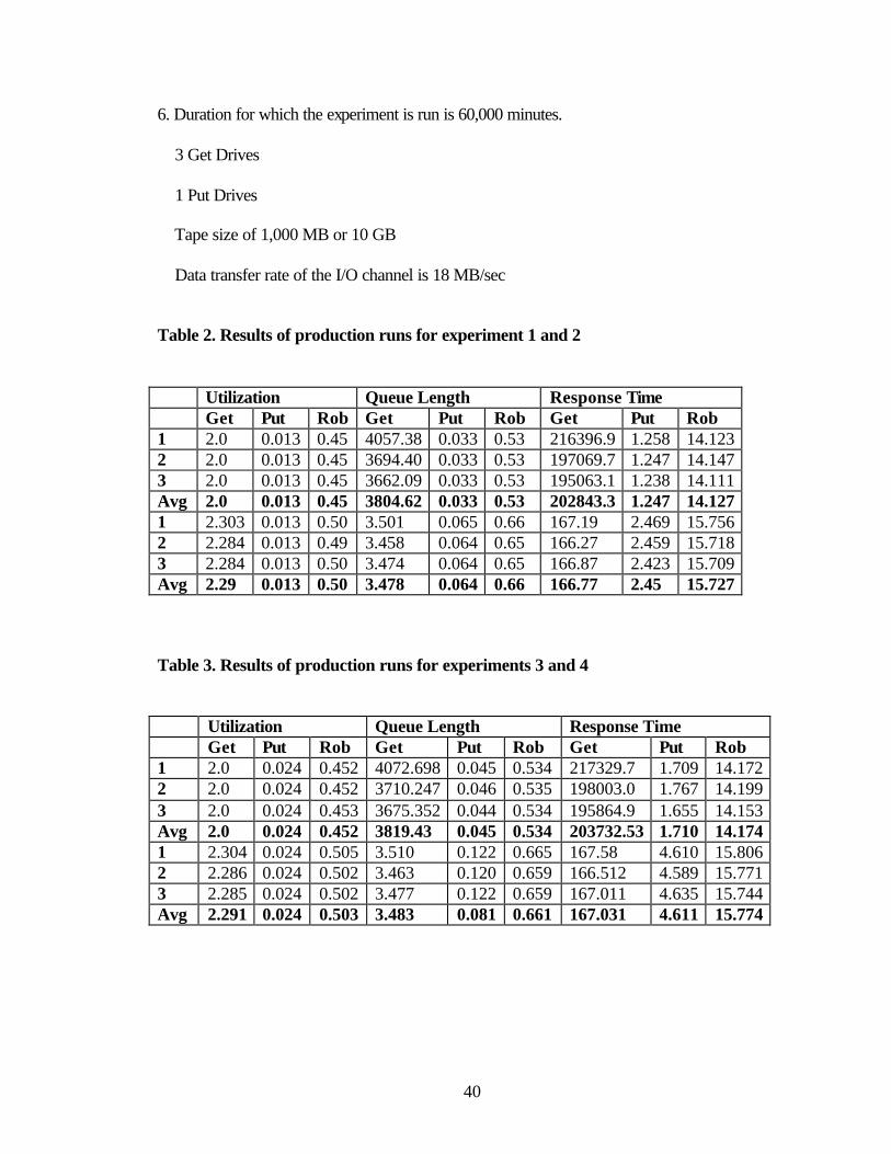
1. Duration for which the experiment is run is 60,000 minutes.

2 Get Drives

2 Put Drives

Tape size of 10,000 MB or 10 GB

Data transfer rate of the I/O channel is 9 MB/sec


3 Get Drives

1 Put Drives



39

Experiments 3 and 4 are used to analyze the system with a small tape size using 2

different type of drive allocations.


2 Get Drives

2 Put Drives




3 Get Drives

1 Put Drives



Experiments 5 and 6 are used to analyze the system with a faster data transfer speed of

the I/O channel compared to all the previous experiments, using 2 different type of drive

allocations.


2 Get Drives

2 Put Drives



40


3 Get Drives

1 Put Drives



Table 2. Results of production runs for experiment 1 and 2 Utilization Queue Length Response Time Get Put Rob Get Put Rob Get Put Rob 1 2.0 0.013 0.45 4057.38 0.033 0.53 216396.9 1.258 14.123 2 2.0 0.013 0.45 3694.40 0.033 0.53 197069.7 1.247 14.147 3 2.0 0.013 0.45 3662.09 0.033 0.53 195063.1 1.238 14.111 Avg 2.0 0.013 0.45 3804.62 0.033 0.53 202843.3 1.247 14.127 1 2.303 0.013 0.50 3.501 0.065 0.66 167.19 2.469 15.756 2 2.284 0.013 0.49 3.458 0.064 0.65 166.27 2.459 15.718 3 2.284 0.013 0.50 3.474 0.064 0.65 166.87 2.423 15.709 Avg 2.29 0.013 0.50 3.478 0.064 0.66 166.77 2.45 15.727 Table 3. Results of production runs for experiments 3 and 4 Utilization Queue Length Response Time Get Put Rob Get Put Rob Get Put Rob 1 2.0 0.024 0.452 4072.698 0.045 0.534 217329.7 1.709 14.172 2 2.0 0.024 0.452 3710.247 0.046 0.535 198003.0 1.767 14.199 3 2.0 0.024 0.453 3675.352 0.044 0.534 195864.9 1.655 14.153 Avg 2.0 0.024 0.452 3819.43 0.045 0.534 203732.53 1.710 14.174 1 2.304 0.024 0.505 3.510 0.122 0.665 167.58 4.610 15.806 2 2.286 0.024 0.502 3.463 0.120 0.659 166.512 4.589 15.771 3 2.285 0.024 0.502 3.477 0.122 0.659 167.011 4.635 15.744 Avg 2.291 0.024 0.503 3.483 0.081 0.661 167.031 4.611 15.774

41

Table 4. Results of production runs for experiments 5 and 6 Utilization Queue Length Response Time Get Put Rob Get Put Rob Get Put Rob 1 2.0 0.007 0.451 4021.127 0.017 0.531 214218.9 0.660 14.124 2 2.0 0.007 0.451 3657.108 0.017 0.531 194863.8 0.65 14.146 3 2.0 0.007 0.451 3626.924 0.017 0.531 192989.9 0.644 14.118 Avg 2.0 0.007 0.451 3768.3 0.017 0.531 200690.9 0.651 14.129 1 2.300 0.007 0.503 3.492 0.036 0.660 166.726 1.369 15.756 2 2.282 0.007 0.499 3.448 0.036 0.654 165.784 1.361 15.718 3 2.282 0.007 0.500 3.465 0.035 0.655 166.442 1.320 15.712 Avg 2.288 0.007 0.500 3.468 0.035 0.656 166.31 1.35 15.728

42

CHAPTER IV

CONCLUSIONS AND FUTURE WORK

From table 2.0 some conclusions are drawn as follows.

1. The first experiment with 2 Get drives and 2 Put drives shows that the Get and Put

drives are busy all the time. Also, the queue lengths for the Get Drives are

exceptionally long. The Response times for the get requests are too large to get

any of the requests processed. As a result this configuration cannot handle the

workload at the FTP server.

2. In the 2nd experiment, the number of Get drives is increased by 1 to a total of 3

Get drives. This results in the Get drives being busy for less percent of time. The

utilization of the Put drives remains almost the same, though the Robot gets busy

by a negligible amount as it has to handle the more number of get drives now.

The Queue length for the Get drives reduced by almost 1100 times. This is a

substantial improvement over experiment one . Also, the response time

decreases by 1200 times. With the reduction in the number of Put drives, the

response times of the Put drives increases, but, is negligible compared to the Get

Drives. The Response times of the Robot increases by a negligible amount. As a

result more number of Get drives is bound to give a better performance.


1. From experiment 3, it is clear that the configuration of 2 Get and 2 Put drives with

a reduction in tape size cannot handle the workload due to long queue lengths and

a huge response time, which is larger compared to the larger tape size.

43

2. From experiment 4, with a smaller tape size, the utilization of the Put drives gets

almost doubled. The reason for this increase is because the empty tape needs to be

mounted and unmounted more number of times as less number of files can be

written on to a smaller tape. At the same time, the queue lengths increases, as

more number of requests have to wait in the Put queue to be processed. The

response times gets almost doubled for smaller tapes. The reason for this is the

time spent in mounting and unmounting the tape for few files each time. Thus, it

can be concluded from these 2 experiments with different tape sizes, that the

larger tape size decreases the utilization, queue length and response times of the

Put drives by 2 fold. Therefore, if the larger tapes are just as expensive as the

smaller tapes it is ideal to use a larger size tape compared to the smaller one. On

the other hand if the larger size makes the tapes very expensive, it is better to use

the smaller tapes, as the results will not vary by a large size.


1. From experiment 5, we can see that the configuration is unsuitable even if the

data transfer rates are doubled. This is because of the large queue sizes and the

huge response time.

2. By comparing experiment 6 with experiment 2 it is clear that the utilization of the

Put drives decreases by almost half as much, i.e, they become less busy, the queue

lengths also get reduced in length by almost half, also the response times get

reduced by half. For the Get drives, the utilization, queue lengths get reduced by a

negligible amount. Therefore, larger data transfer rates do improve the

performance.

44

The overall conclusion drawn from all the above experiments is that, when cost is

the criteria, it is best to increase the number of Get drives to get the best

results. If cost is not that important, it is better to increase the data transfer rates

along with the tape size, to get better performance.

The future work in this area, could concentrate on conducting more number of

experiments with a variety of other configurations of drive allocations and

varying many other parameters which have been used as constants in the

experiment. Also, the model only simulates the tape library, it is better to add the

external elements like disc cache and experiment the model as a whole to see the

effects of caching.

45

APPENDIX A

46

USER MANUAL

The model is simulated using only one file named model.c in the UNIX environment. It

has all the functions to handle the ARM archive requests using the IBM 3494 Automated

Tape library.

At the Unix prompt type:

<Agassiz:~/csim/examples>$ sh robot

The file robot is a script file, the contents of the file are as below.

./csim model.c

./a.out<dat>outfile

./a.out<dat1>>outfile




The dat, dat1, dat2…. files are the data files used as various input cases for the model.

The contents of the dat file are

60000 2 2 10000 9

This implies that the model is simulated for 60000 minutes, using 2 get drives, 2 put

drives with 10000 MB tape size and a transfer rate of 9 MB/sec. The data file makes it

easier to run the model more than once.

The statement ./a.out<dat>outfile writes the output to the outfile.

47

CSIM produces reports indicating usage and queing information on facilities and storage

blocks. It also collects summary information from tables, qtables, histograms and

qhistograms, if any were created in the program.

The model generates reports on facilities and tables using report_facilities() and

report_tables(). Report_facilities() prints the usage statistics for all facilities defined in

the model namely robot(single server facility), get drives and put drives(multi-server

facility).

The subparts of the report_facilities() command are as follows.

Output Heading Facility Usage Statistics

General Information

facility Name (for a facility set , the index is appended).eg. Robot

srv Server number (for facilities with multiple servers).eg.0,1

disp Service discipline (when one was defined) eg. fcfs by default.

Means

Serv_tm Mean service time per request

util Mean utilization(busy time devided by elapsed time)

tput Mean throughput rate(completions per unit time)

qlen Mean number of requests waiting or in service

resp mean time at facility (both waiting and in service)

Counts

cmp Number of requests completed

pre Number of preemptions which occurred

48

Report_Tables Output

Qtables and Qhistograms ( also output by report_qtable(qt)

Mean queue length Mean number of processes in queue (note_entry has

occurred, but a note_exit has not)

Mean time in queue Mean time between note_entry and note_exit

Max queue length Maximum number of processes in queue

Number of entries Number of note_entry’s and note_exit’s devided by 2

Similarly dat2 looks like 60000 3 1 10000 9

Dat3 looks like 60000 2 2 1000 9

Dat4 looks like 60000 3 1 1000 9

Dat5 looks like 60000 2 2 10000 18

Dat6 looks like 60000 3 1 10000 18

By observing the usage statistics collected by the program results are concluded.

49

APPENDIX B

50

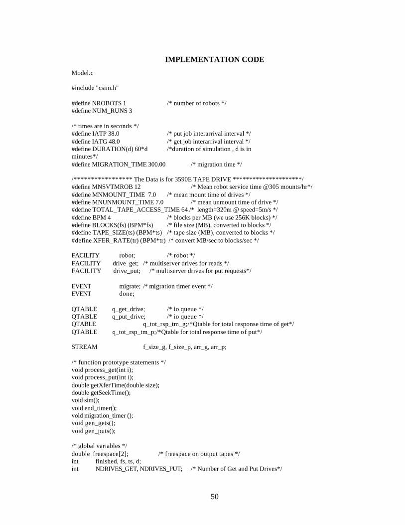
IMPLEMENTATION CODE

Model.c #include "csim.h" #define NROBOTS 1 /* number of robots */ #define NUM_RUNS 3 /* times are in seconds */ #define IATP 38.0 /* put job interarrival interval */ #define IATG 48.0 /* get job interarrival interval */ #define DURATION(d) 60*d /*duration of simulation , d is in minutes*/ #define MIGRATION_TIME 300.00 /* migration time */ /***************** The Data is for 3590E TAPE DRIVE *********************/ #define MNSVTMROB 12 /* Mean robot service time @305 mounts/hr*/ #define MNMOUNT_TIME 7.0 /* mean mount time of drives */ #define MNUNMOUNT_TIME 7.0 /* mean unmount time of drive */ #define TOTAL_TAPE_ACCESS_TIME 64 /* length=320m @ speed=5m/s */ #define BPM 4 /* blocks per MB (we use 256K blocks) */ #define BLOCKS(fs) (BPM*fs) /* file size (MB), converted to blocks */ #define TAPE_SIZE(ts) (BPM*ts) /* tape size (MB), converted to blocks */ #define XFER_RATE(tr) (BPM*tr) /* convert MB/sec to blocks/sec */ FACILITY robot; /* robot */ FACILITY drive_get; /* multiserver drives for reads */ FACILITY drive_put; /* multiserver drives for put requests*/ EVENT migrate; /* migration timer event */ EVENT done; QTABLE q_get_drive; /* io queue */ QTABLE q_put_drive; /* io queue */ QTABLE q_tot_rsp_tm_g;/*Qtable for total response time of get*/ QTABLE q_tot_rsp_tm_p;/*Qtable for total response time of put*/ STREAM f_size_g, f_size_p, arr_g, arr_p; /* function prototype statements */ void process_get(int i); void process_put(int i); double getXferTime(double size); double getSeekTime(); void sim(); void end_timer(); void migration_timer (); void gen_gets(); void gen_puts(); /* global variables */ double freespace[2]; /* freespace on output tapes */ int finished, fs, ts, d; int NDRIVES_GET, NDRIVES_PUT; /* Number of Get and Put Drives*/

51

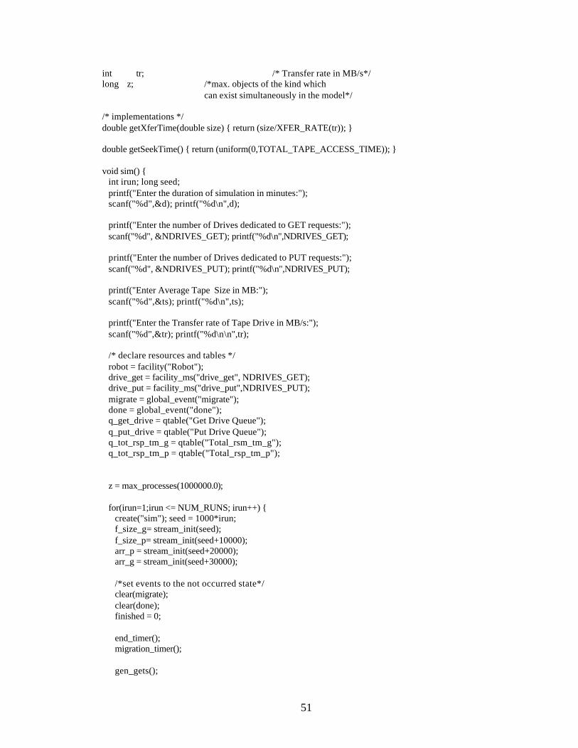
int tr; /* Transfer rate in MB/s*/ long z; /*max. objects of the kind which can exist simultaneously in the model*/ /* implementations */ double getXferTime(double size) { return (size/XFER_RATE(tr)); } double getSeekTime() { return (uniform(0,TOTAL_TAPE_ACCESS_TIME)); } void sim() { int irun; long seed; printf("Enter the duration of simulation in minutes:"); scanf("%d",&d); printf("%d\n",d); printf("Enter the number of Drives dedicated to GET requests:"); scanf("%d", &NDRIVES_GET); printf("%d\n",NDRIVES_GET); printf("Enter the number of Drives dedicated to PUT requests:"); scanf("%d", &NDRIVES_PUT); printf("%d\n",NDRIVES_PUT); printf("Enter Average Tape Size in MB:"); scanf("%d",&ts); printf("%d\n",ts); printf("Enter the Transfer rate of Tape Drive in MB/s:"); scanf("%d",&tr); printf("%d\n\n",tr); /* declare resources and tables */ robot = facility("Robot"); drive_get = facility_ms("drive_get", NDRIVES_GET); drive_put = facility_ms("drive_put",NDRIVES_PUT); migrate = global_event("migrate"); done = global_event("done"); q_get_drive = qtable("Get Drive Queue"); q_put_drive = qtable("Put Drive Queue"); q_tot_rsp_tm_g = qtable("Total_rsm_tm_g"); q_tot_rsp_tm_p = qtable("Total_rsp_tm_p"); z = max_processes(1000000.0); for(irun=1;irun <= NUM_RUNS; irun++) { create("sim"); seed = 1000*irun; f_size_g= stream_init(seed); f_size_p= stream_init(seed+10000); arr_p = stream_init(seed+20000); arr_g = stream_init(seed+30000); /*set events to the not occurred state*/ clear(migrate); clear(done); finished = 0; end_timer(); migration_timer(); gen_gets();

52

gen_puts(); wait(done); printf("=============================\n"); printf("*****Run Number = %d*****\n", irun); printf("=============================\n"); report_facilities(); report_tables(); rerun(); } //end of for loop } void end_timer() { create("end_timer"); hold(DURATION(d)); finished = 1; set(done); } void migration_timer() { long r; create("timer"); while (finished == 0) { /*Wait for the migrate event,but,only till migration_time*/ r = timed_wait(migrate, MIGRATION_TIME); set(migrate); clear(migrate); } } void gen_gets() { int i=0; double iat; create("gen_gets"); while (finished == 0) { process_get(++i); iat=stream_expntl(arr_g,IATG); hold(iat); } } void gen_puts() { double iat; int i=0; create("gen_puts"); while (finished == 0) { process_put(++i); iat=stream_expntl(arr_p,IATP); hold(iat); } } void process_get(int i) {

53

double t1, f_size, XferTime,SeekTime,RewindTime; long unit; create("get"); set_priority(1); /*Set priority for the get process*/ f_size = stream_uniform(f_size_g,BLOCKS(1),BLOCKS(3.2)); XferTime = getXferTime(f_size); SeekTime = getSeekTime(); RewindTime = SeekTime; t1 = MNMOUNT_TIME+SeekTime+XferTime+RewindTime+MNUNMOUNT_TIME; note_entry(q_tot_rsp_tm_g); note_entry(q_get_drive); unit = reserve(drive_get); /*reserve a tape drive for get request*/ note_exit(q_get_drive); use(robot,MNSVTMROB); /*use the robot to load the tape */ hold(t1); use(robot,MNSVTMROB); release_server(drive_get, unit); note_exit(q_tot_rsp_tm_g); } void process_put(int i) { long unit; double f_size, XferTime,SeekTime; create("put"); f_size = stream_uniform(f_size_p,BLOCKS(0.5),BLOCKS(7.5)); XferTime = getXferTime(f_size); set_priority(0); /*Set priority for the put process*/ note_entry(q_tot_rsp_tm_p); wait(migrate); note_entry(q_put_drive); unit = reserve(drive_put); if (freespace[unit]<f_size) { /* store full tape, mount new tape */ hold (64); /* rewind the tape */ hold(MNUNMOUNT_TIME); use(robot,MNSVTMROB); /* robot unloads the tape*/ use(robot,MNSVTMROB); /* robot loads new tape into drive */ hold(MNMOUNT_TIME); freespace[unit] = TAPE_SIZE(ts); /* reset remaining tape capacity */ } hold(XferTime); freespace[unit] = freespace[unit] - f_size; release_server(drive_put, unit); note_exit(q_put_drive); note_exit(q_tot_rsp_tm_p); }

54

Script file: robot ./csim model.c ./a.out<dat1>outfile ./a.out<dat2>>outfile ./a.out<dat3>>outfile ./a.out<dat4>>outfile ./a.out<dat5>>outfile ./a.out<dat6>>outfile Dat files Dat1 60000 2 2 10000 9 Dat2 60000 3 1 10000 9 Dat3 60000 2 2 1000 9 Dat4 60000 3 1 1000 9 Dat5 60000 2 2 10000 18 Dat6 60000 3 1 10000 18

55

REFERENCES

[1] Tugrul Dayar,Odysseas I.Pentakalos,and A.B.Stephens: Analytical modeling of

Robotic Tape Libraries using stochastic Automata

[2] Toshihiro Nemoto,Mesaru Kitsuregawa,Mikio Takagi :Design and Implementation of

Scalable Tape Archiver

[3] Theodore Johnson: Queuing Models of Tertiary Storage

[4] Leana Golubchik and Richard R. Muntz : Analysis of Striping Techniques in Robotic

Storage Libraries

[5] Theodore Johnson : Analysis of the Request patterns to the NSSDC On-line Archive

[6] Odysseas I. Pentakalos,Daniel A. Menasce, Milt Halem, Yalena Yesha : Analytical

Performance Modeling of Hierachical Mass Storage Systems

[7] Product Description. Ampex DST800 automated catridge library.

[8] S.Ranade,ed., Jukebox and Robotic Libraries for Computer Mass Storage ,Meckler,

1992.

[9] Elias Drakopoulos and Matt J. Merges: Performance Analysis of Client –Server

Storage systems ,IEEE Transactions on Computers ,Vol.41,No.11,pp.1442-1452,19992.

[10] Daniel A. Menasce, Odyseas I. Pentakalos,and Yalena Yesha: An Analytical Model

of Hierarchical Mass Storage Systems with Network-Attached Storage Devices “ in

SIGMETRICS 96,Philadelphia,PA,May 23-26,pp.180-189,1996.

[10] Elias Drakopoulos and Matt J. Merges : Performance Study of Client-Server Storage

Systems in Eleventh IEEE symposium on Mass Storage Systems,Monterey ,

California,pp. 67-72,1991.

56

[11] Ann L. Drapeau and Randy H. Katz: Striped Tape Arrays, in Twelth IEEE

Symposium on Mass storage Systems,Monterey, California,pp.257-265,1993.

[12] Theodore Johnson: An Analytical Performance Model of Robotic Storage Libraries,

in Performance 96,Lausanne,Switzerland, October 7-11 1996.

[13] http://www.archive.arm.gov/stats/ for Atmospheric Radiation Measurement data and

usage statistics.

[14] http://www.storage.ibm.com/hardsoft/tape/3494/ for specification of IBM 3494 Tape

Library.

[15] http://www.storage.ibm.com/hardsoft/tape/3494/prod_data/g225-6601.html for

information on IBM Magstar 3494 Tape Library.

[16] http://www.sdsc.edu/hpss/hpss1.html for a tutorial on High Performance Storage

System.

[17] http://www.sdsc.edu/hpss/HPSS_overview.html for an overview on HPSS.

[18] Software Engineering – Roger S Pressman for Software Engineering techniques,

design and implementation.

[19] Measuring Tape Drive Performance, Theodore Johnson, att.tjohnson.981013

[20] http://www-hppc.final.gov/rip/tapetests/results.html for Tape Drive Measured

Results

Documents

SIMULATION OF IBM 3494 AUTOMATED TAPE LIBRARY …media.aero.und.edu/cs.und.edu/documents/ShantiSwarupa.pdf · SIMULATION OF IBM 3494 AUTOMATED TAPE LIBRARY ... Level 0 Data Flow Diagram