Embed Size (px)
Citation preview
Degree project
Simulation of 3ph induction motor in Matlab
with Direct and Soft starting methods
Author: Mohamad Moulham Abboud
Supervisor: Matz Lenells
Examiner: Pieternella Cijvat
Date: 15-06-04
Course code: 2ED14E, 15 hp
Topic: Electrical Engineering
Level: Bachelor of Science
Department of Physics and
Electrical Engineering
Faculty of Technology

1

2
Abstract
Asynchronous machines are considered nowadays the most commonly used electrical
machines, which are mainly used as electrical induction motors. Starting the induction motor
is the most important and dangerous step. The theory behind this project is based on
representing the real motor by a set of equations and values in Matlab using the subsystem
feature, forming a corresponding idealistic motor in a way where all the physical effects are
similar. The motor is started under different loads in two methods: Direct and Soft starting.
Each method is studied and discussed using supporting simulation of currents, torque, speed,
efficiency and power factor curves.
Keywords: 3ph-induction motor, Matlab, Model, Simulation, Direct starting, Soft starting.

3
Acknowledgement
I am grateful to God for the support, good health and wellbeing that were necessary to
complete this project. I feel deeply honored expressing my sincere thanks to Matz Lenells for
providing valuable insights leading to the successful completion of my project. I take this
opportunity to express gratitude to all of the department faculty members for their help and
support. I also thank my loving family and friends for the encouragement, support and
attention through this venture.
4
Table of contents
Abstract ……………………………………………………………………...……..………….…2
Acknowledgment……………………………………………………..…………………….…….3
1. Introduction ………………………………………………………………………………….5
Problem formulation ……… ……………………………………………………..…………….5
2. A General Outline of Induction Motors ………………………………………….…………6
2,1. The 3ph induction motor structure ………..…….…….......…………………….....6
2.2. Basic Theory of Three Phase Induction Motors....................................…...............8
3. The general theory of electrical machines ………………………...……………….............11
4. Simulating and starting the 3ph induction motor in Matlab…………….…………..….…...13
4.A. The induction motor model...................................................................................13
4. B. Simulating starting curves in No-load \ Load cases……...…………...…...........16
4. C. Direct starting method………………………………….………………..….......17
4. C.1. Direct starting curves in the No-load case……………….……..........18
4. C.2 Direct starting curves in the 75% of nominal load case ………...........19
4. C.3 Direct starting curves in the nominal load case.………...……............22
5. Soft staring method………………………………………………………………..……......25
5.1 Soft starting curves in the nominal load case……………….…………………....26
5.2 Soft starting curves in the 75% of nominal load case…….………………….......29
5.3 Soft starting curves in the 50% of nominal load case……….……………….......31
5.4 Soft starting curves in the 25% of nominal load case…….……………………...34
6. Conclusions and discussion…...……………………………………….……………...…...37
References ……………………………………....………………………...………………....39
Appendix 1………….……………………………………..……………………………...…..40
Notes……………………………………………………………………………….....40
Matlab code……………………………………………………………………....…..40
Glossary of symbols……………………………………………...…………………..41
Appendix 2………….……………………………………..……………………………...…..42
5
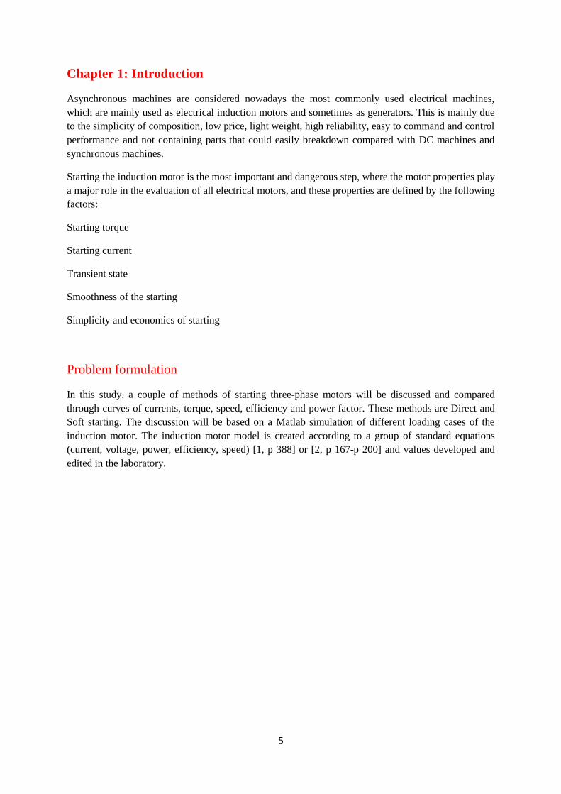
Chapter 1: Introduction
Asynchronous machines are considered nowadays the most commonly used electrical machines,
which are mainly used as electrical induction motors and sometimes as generators. This is mainly due
to the simplicity of composition, low price, light weight, high reliability, easy to command and control
performance and not containing parts that could easily breakdown compared with DC machines and
synchronous machines.
Starting the induction motor is the most important and dangerous step, where the motor properties play
a major role in the evaluation of all electrical motors, and these properties are defined by the following
factors:
Starting torque
Starting current
Transient state
Smoothness of the starting
Simplicity and economics of starting
Problem formulation
In this study, a couple of methods of starting three-phase motors will be discussed and compared
through curves of currents, torque, speed, efficiency and power factor. These methods are Direct and
Soft starting. The discussion will be based on a Matlab simulation of different loading cases of the
induction motor. The induction motor model is created according to a group of standard equations
(current, voltage, power, efficiency, speed) [1, p 388] or [2, p 167-p 200] and values developed and
edited in the laboratory.
6
Chapter 2: A General Outline of Induction Motors
2.1 The 3ph induction motor structure:
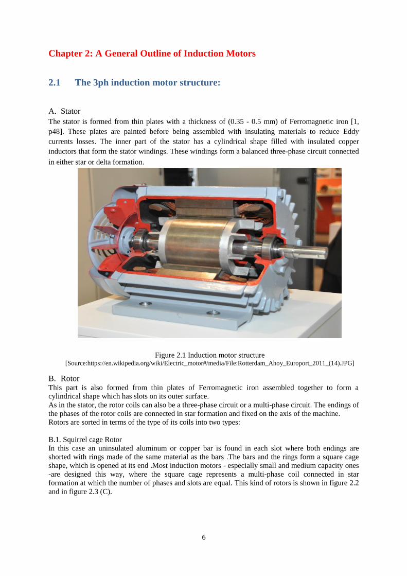
A. Stator
The stator is formed from thin plates with a thickness of (0.35 - 0.5 mm) of Ferromagnetic iron [1,
p48]. These plates are painted before being assembled with insulating materials to reduce Eddy
currents losses. The inner part of the stator has a cylindrical shape filled with insulated copper
inductors that form the stator windings. These windings form a balanced three-phase circuit connected
in either star or delta formation.
Figure 2.1 Induction motor structure [Source:https://en.wikipedia.org/wiki/Electric_motor#/media/File:Rotterdam_Ahoy_Europort_2011_(14).JPG]
B. Rotor This part is also formed from thin plates of Ferromagnetic iron assembled together to form a
cylindrical shape which has slots on its outer surface.
As in the stator, the rotor coils can also be a three-phase circuit or a multi-phase circuit. The endings of
the phases of the rotor coils are connected in star formation and fixed on the axis of the machine.
Rotors are sorted in terms of the type of its coils into two types:
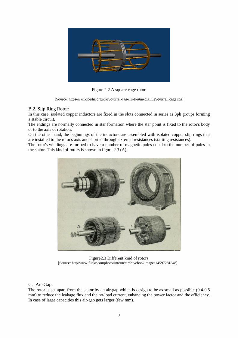
B.1. Squirrel cage Rotor
In this case an uninsulated aluminum or copper bar is found in each slot where both endings are
shorted with rings made of the same material as the bars .The bars and the rings form a square cage
shape, which is opened at its end .Most induction motors - especially small and medium capacity ones
-are designed this way, where the square cage represents a multi-phase coil connected in star
formation at which the number of phases and slots are equal. This kind of rotors is shown in figure 2.2
and in figure 2.3 (C).
7
Figure 2.2 A square cage rotor
[Source: httpsen.wikipedia.orgwikiSquirrel-cage_rotor#mediaFileSquirrel_cage.jpg]
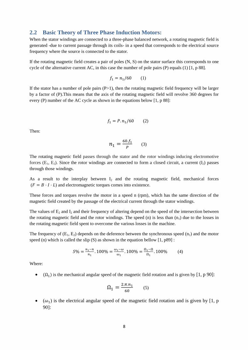
B.2. Slip Ring Rotor: In this case, isolated copper inductors are fixed in the slots connected in series as 3ph groups forming
a stable circuit.
The endings are normally connected in star formation where the star point is fixed to the rotor's body
or to the axis of rotation.
On the other hand, the beginnings of the inductors are assembled with isolated copper slip rings that
are installed to the rotor's axis and shorted through external resistances (starting resistances).
The rotor's windings are formed to have a number of magnetic poles equal to the number of poles in
the stator. This kind of rotors is shown in figure 2.3 (A).
Figure2.3 Different kind of rotors [Source: httpswww.flickr.comphotosinternetarchivebookimages14597281848]
C. Air-Gap: The rotor is set apart from the stator by an air-gap which is design to be as small as possible (0.4-0.5
mm) to reduce the leakage flux and the no-load current, enhancing the power factor and the efficiency.
In case of large capacities this air-gap gets larger (few mm).
8
2.2 Basic Theory of Three Phase Induction Motors: When the stator windings are connected to a three-phase balanced network, a rotating magnetic field is
generated -due to current passage through its coils- in a speed that corresponds to the electrical source
frequency where the source is connected to the stator.
If the rotating magnetic field creates a pair of poles (N, S) on the stator surface this corresponds to one
cycle of the alternative current AC, in this case the number of pole pairs (P) equals (1) [1, p 88].
𝑓1 = 𝑛1/60 (1)
If the stator has a number of pole pairs (P>1), then the rotating magnetic field frequency will be larger
by a factor of (P).This means that the axis of the rotating magnetic field will revolve 360 degrees for
every (P) number of the AC cycle as shown in the equations below [1, p 88]:
𝑓1 = 𝑃. 𝑛1/60 (2)
Then:
𝑛1 =60.𝑓1
𝑃 (3)
The rotating magnetic field passes through the stator and the rotor windings inducing electromotive
forces (E1, E2). Since the rotor windings are connected to form a closed circuit, a current (I2) passes
through those windings.
As a result to the interplay between I2 and the rotating magnetic field, mechanical forces
(𝐹 = 𝐵 · 𝐼 · 𝐿) and electromagnetic torques comes into existence.
These forces and torques revolve the motor in a speed n (rpm), which has the same direction of the
magnetic field created by the passage of the electrical current through the stator windings.
The values of E2 and I2 and their frequency of altering depend on the speed of the intersection between
the rotating magnetic field and the rotor windings. The speed (n) is less than (n1) due to the losses in
the rotating magnetic field spent to overcome the various losses in the machine.
The frequency of (E1, E2) depends on the deference between the synchronous speed (n1) and the motor
speed (n) which is called the slip (S) as shown in the equation bellow [1, p89] :
𝑆% =𝑛1−𝑛
𝑛1. 100% =
𝜔1−𝜔
𝜔1. 100% =
Ω1−Ω
Ω1. 100% (4)
Where:
(Ω1) is the mechanical angular speed of the magnetic field rotation and is given by [1, p 90]:
Ω1 =2.𝜋.𝑛1
60 (5)
(𝜔1) is the electrical angular speed of the magnetic field rotation and is given by [1, p
90]:
9
𝜔1 = Ω1. 𝑃 =2.𝜋.𝑛1
60. 𝑃 = 2. 𝜋. 𝑓1 (6)
( ) is the mechanical angular speed of the motor and is given by [1, p 90]:
Ω =2.𝜋.𝑛
60 (7)
(𝜔) is the electrical angular speed of the motor. Therefore [1, p91]:
𝑛 = (1 − 𝑆). 𝑛1 (8)
𝜔 = (1 − 𝑆).𝜔1 (9)
The rotor does not revolve synchronically with the magnetic field (𝑛 ≠ 𝑛1) and this is where the name
"Asynchronous motors" comes from. This type of motors is also called "induction motors" because the
current that passes through the rotor is created in an inductive way that is not given from an external
source.
In order to calculate (𝑓2) for (E2), (I2) and a speed (𝑛1 − 𝑛) it is found that [1, p92]:
𝑓2 =(𝑛1−𝑛).𝑃
60 (10)
But:
𝑆 =𝑛1−𝑛
𝑛1 (11)
Therefore:
𝑓1 =𝑃.𝑛1
60 (12)
The electromotive forces (emf) induced in the stator and rotor winding are given by the equations [1, p
95]:
𝐸1 = 4.44 ∙ 𝑓1 ∙ 𝑊𝑝ℎ1 ∙ 𝜙 ∙ 𝐾𝑊1 (13)
𝐸2𝑆 = 4.44 ∙ 𝑓2 ∙ 𝑊𝑝ℎ2 ∙ 𝜙 ∙ 𝐾𝑊2 (14)
Where (𝐸2𝑆) is the emf induced in the rotor windings when revolving with a slip (S) and is also given
by the equation [1, p 95]:
𝐸2𝑆 = 4.44 ∙ 𝑓2 ∙ 𝑊𝑝ℎ2 ∙ 𝜙 ∙ 𝐾𝑊2=4.44 ∙ 𝑆 ∙ 𝑓1 ∙ 𝑊𝑝ℎ2 ∙ 𝜙 ∙ 𝐾𝑊2 = 𝑆 ∙ 𝐸2 (15)
The values of the slip (S) are determined by the mechanical load applied to the rotation axis. It
increases proportionally with the load (the speed decreases).
10
But if the motor would revolve in the synchronous speed (𝑛 = 𝑛1) and in the same direction (𝑆 = 0),
the magnetic field would not have crossed the rotor winding, therefore no emf would have been
induced in the rotor and no current would have passed in the rotor windings. Thus, neither
mechanical forces nor rotating torques would have come into existence.
As a conclusion, the induction motor should revolve in a speed less than the synchronous speed in
order for it to work as a motor, therefore its domain is limited by the following conditions [1, p
96]:
𝑛1 > 𝑛 > 0 (16)
1 > 𝑆 > 0 (17)
11
Chapter 3: The general theory of electrical machines:
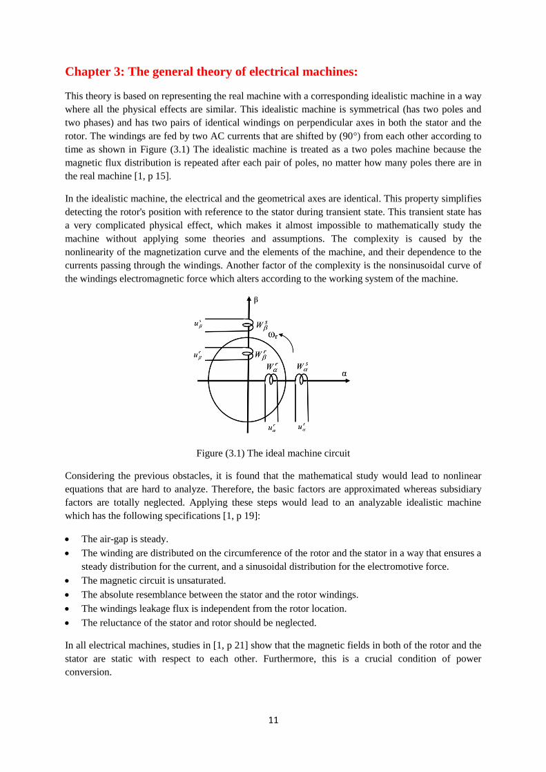
This theory is based on representing the real machine with a corresponding idealistic machine in a way
where all the physical effects are similar. This idealistic machine is symmetrical (has two poles and
two phases) and has two pairs of identical windings on perpendicular axes in both the stator and the
rotor. The windings are fed by two AC currents that are shifted by (90°) from each other according to
time as shown in Figure (3.1) The idealistic machine is treated as a two poles machine because the
magnetic flux distribution is repeated after each pair of poles, no matter how many poles there are in
the real machine [1, p 15].
In the idealistic machine, the electrical and the geometrical axes are identical. This property simplifies
detecting the rotor's position with reference to the stator during transient state. This transient state has
a very complicated physical effect, which makes it almost impossible to mathematically study the
machine without applying some theories and assumptions. The complexity is caused by the
nonlinearity of the magnetization curve and the elements of the machine, and their dependence to the
currents passing through the windings. Another factor of the complexity is the nonsinusoidal curve of
the windings electromagnetic force which alters according to the working system of the machine.
Figure (3.1) The ideal machine circuit
Considering the previous obstacles, it is found that the mathematical study would lead to nonlinear
equations that are hard to analyze. Therefore, the basic factors are approximated whereas subsidiary
factors are totally neglected. Applying these steps would lead to an analyzable idealistic machine
which has the following specifications [1, p 19]:
The air-gap is steady.
The winding are distributed on the circumference of the rotor and the stator in a way that ensures a
steady distribution for the current, and a sinusoidal distribution for the electromotive force.
The magnetic circuit is unsaturated.
The absolute resemblance between the stator and the rotor windings.
The windings leakage flux is independent from the rotor location.
The reluctance of the stator and rotor should be neglected.
In all electrical machines, studies in [1, p 21] show that the magnetic fields in both of the rotor and the
stator are static with respect to each other. Furthermore, this is a crucial condition of power
conversion.
12
When running electrical machines, a few phenomena occur and it is required to represent these
phenomena as mathematical equations in order to study the machine. These equations depend on each
other, but one can, anyway, consider them to belong to one of three groups which describe [1, p 22]:
The windings voltages.
The torques on the axis of the machine.
The mechanical motion.
In order for these equations to be written in a standard way, it is important to consider the following
[1, p 23]:
The positive direction of the current passing through the windings is from the windings ending
towards its beginning.
The electromotive force has the same positive direction as the current.
The positive direction of the magnetic flux is the direction of the flux coming out of the rotor.
The positive direction of the winding axes and the electromagnetic force is the same positive
direction of the current.
The positive direction of the machine revolution, the electromotive force and the angles
calculation is counter clockwise.
To be able to study the mathematical model, it is customary to choose one of the following rectangular
coordinates that are commonly used in this case [1, p 24]:
1. The coordinates system of (α) and (β) which is fixed on the stator.
2. The coordinates system of (d) and (q) which is fixed on the rotor and revolves with it in the same
speed.
3. The coordinates system of (u) and (v) which is fixed on optional coordinates and revolves in an
optional speed as well.
The power conversion process in electrical machines does not depend on choosing the coordinates
system. However, it is preferred to use the (α) and (β) coordinates system to study power conversion
equations, because the voltage equations in the stator have a minimum number of terms.
Furthermore, the observer is static in reference to the stator and the frequency of the network voltage
in this coordinates system.
13
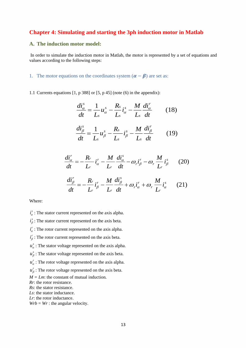
Chapter 4: Simulating and starting the 3ph induction motor in Matlab
A. The induction motor model: In order to simulate the induction motor in Matlab, the motor is represented by a set of equations and
values according to the following steps:
1. The motor equations on the coordinates system (𝜶 − 𝜷) are set as:
1.1 Currents equations [1, p 388] or [5, p 45] (note (6) in the appendix):
(18) 1
dt
di
L
Mi
L
Ru
Ldt
di r
s
s
s
ss
s
s
(19) 1
dt
di
L
Mi
L
Ru
Ldt
di r
s
s
s
ss
s
s
(20) s
rr
r
r
s
r
r
r
rr
iL
Mi
dt
di
L
Mi
L
R
dt
di
(21) s
rr
r
r
s
r
r
r
rr
iL
Mi
dt
di
L
Mi
L
R
dt
di
Where:
si : The stator current represented on the axis alpha.
si : The stator current represented on the axis beta.
ri : The rotor current represented on the axis alpha.
ri : The rotor current represented on the axis beta.
su : The stator voltage represented on the axis alpha.
su : The stator voltage represented on the axis beta.
ru : The rotor voltage represented on the axis alpha.
ru : The rotor voltage represented on the axis beta.
M = Lm: the constant of mutual induction.
Rr: the rotor resistance.
Rs: the stator resistance.
Ls: the stator inductance.
Lr: the rotor inductance.
Wrb = Wr : the angular velocity.
14
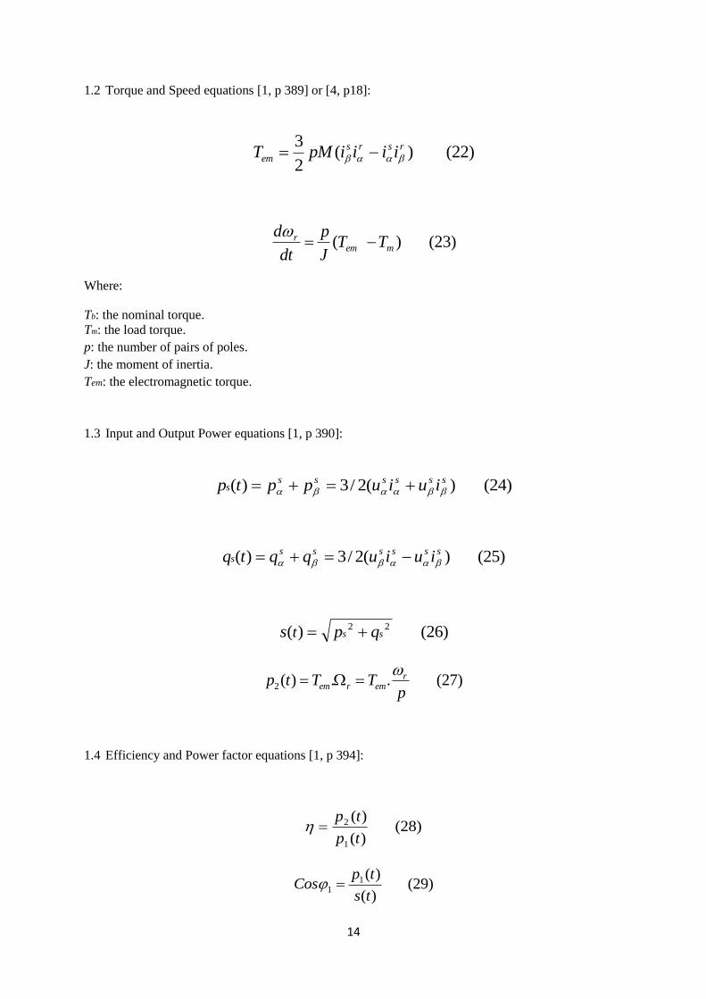
1.2 Torque and Speed equations [1, p 389] or [4, p18]:
(22) )(2
3 rsrs
em iiiipMT
(23) )( memr TT
J
p
dt
d
Where:
Tb: the nominal torque.
Tm: the load torque.
p: the number of pairs of poles.
J: the moment of inertia.
Tem: the electromagnetic torque.
1.3 Input and Output Power equations [1, p 390]:
(24) )(2/3)( sssssss iuiupptp
(25) )(2/3)( sssssss iuiuqqtq
(26) )( 22ss qps t
(27) ..)(2p
TTtp remrem
1.4 Efficiency and Power factor equations [1, p 394]:
(28) )(
)(
1
2
tp
tp
(29) )(
)(11
ts
tpCos
15
Where:
Pn: real power in kw. sp : The stator real power represented on the axis alpha.
sp : The stator real power represented on the axis beta.
q: reactive power. sq : The stator reactive power represented on the axis alpha.
sq : The stator reactive power represented on the axis beta.
s: apparent power.
p1(t): the electrical power (input of the motor).
p2(t): the mechanical power (output of the motor).
1Cos : the power factor.
: the efficiency.
r :the mechanical angular speed.
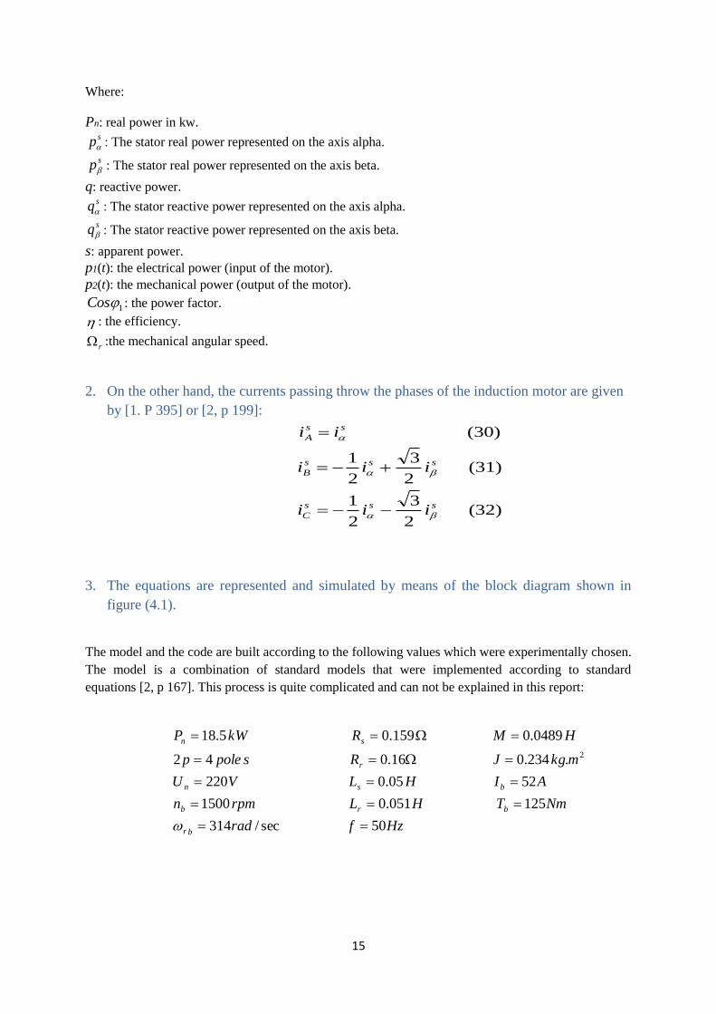
2. On the other hand, the currents passing throw the phases of the induction motor are given
by [1. P 395] or [2, p 199]:
3. The equations are represented and simulated by means of the block diagram shown in
figure (4.1).
The model and the code are built according to the following values which were experimentally chosen.
The model is a combination of standard models that were implemented according to standard
equations [2, p 167]. This process is quite complicated and can not be explained in this report:
Hzfrad
NmTHLrpmn
AIHLVU
mkgJRspolep
HMRkWP
br
brb
bsn
r
sn
50 sec/314
125 051.0 1500
52 05.0 220
.234.0 16.0 42
0489.0 159.0 5.18
2
(32) 2
3
2
1
(31) 2
3
2
1
(30)
sss
C
sss
B
ss
A
iii
iii
ii
16
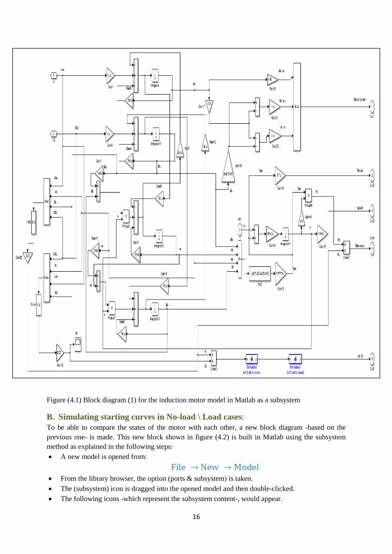
Figure (4.1) Block diagram (1) for the induction motor model in Matlab as a subsystem
B. Simulating starting curves in No-load \ Load cases:
To be able to compare the states of the motor with each other, a new block diagram -based on the
previous one- is made. This new block shown in figure (4.2) is built in Matlab using the subsystem
method as explained in the following steps:
A new model is opened from:
From the library browser, the option (ports & subsystem ( is taken.
The (subsystem) icon is dragged into the opened model and then double-clicked.
The following icons -which represent the subsystem content-, would appear.
17
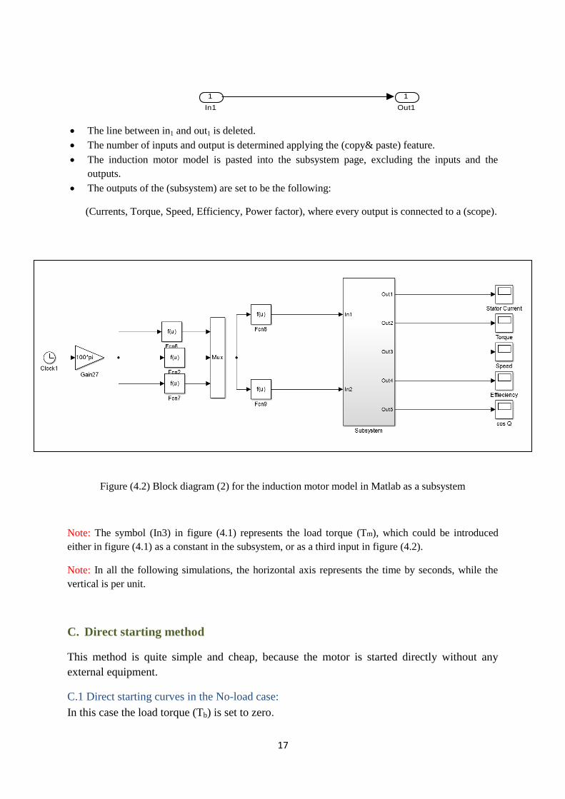
The line between in1 and out1 is deleted.
The number of inputs and output is determined applying the (copy& paste) feature.
The induction motor model is pasted into the subsystem page, excluding the inputs and the
outputs.
The outputs of the (subsystem) are set to be the following:
(Currents, Torque, Speed, Efficiency, Power factor), where every output is connected to a (scope).
Figure (4.2) Block diagram (2) for the induction motor model in Matlab as a subsystem
Note: The symbol (In3) in figure (4.1) represents the load torque (Tm), which could be introduced
either in figure (4.1) as a constant in the subsystem, or as a third input in figure (4.2).
Note: In all the following simulations, the horizontal axis represents the time by seconds, while the
vertical is per unit.
C. Direct starting method
This method is quite simple and cheap, because the motor is started directly without any
external equipment.
C.1 Direct starting curves in the No-load case:
In this case the load torque (Tb) is set to zero.
1
Out1
1
In1
18
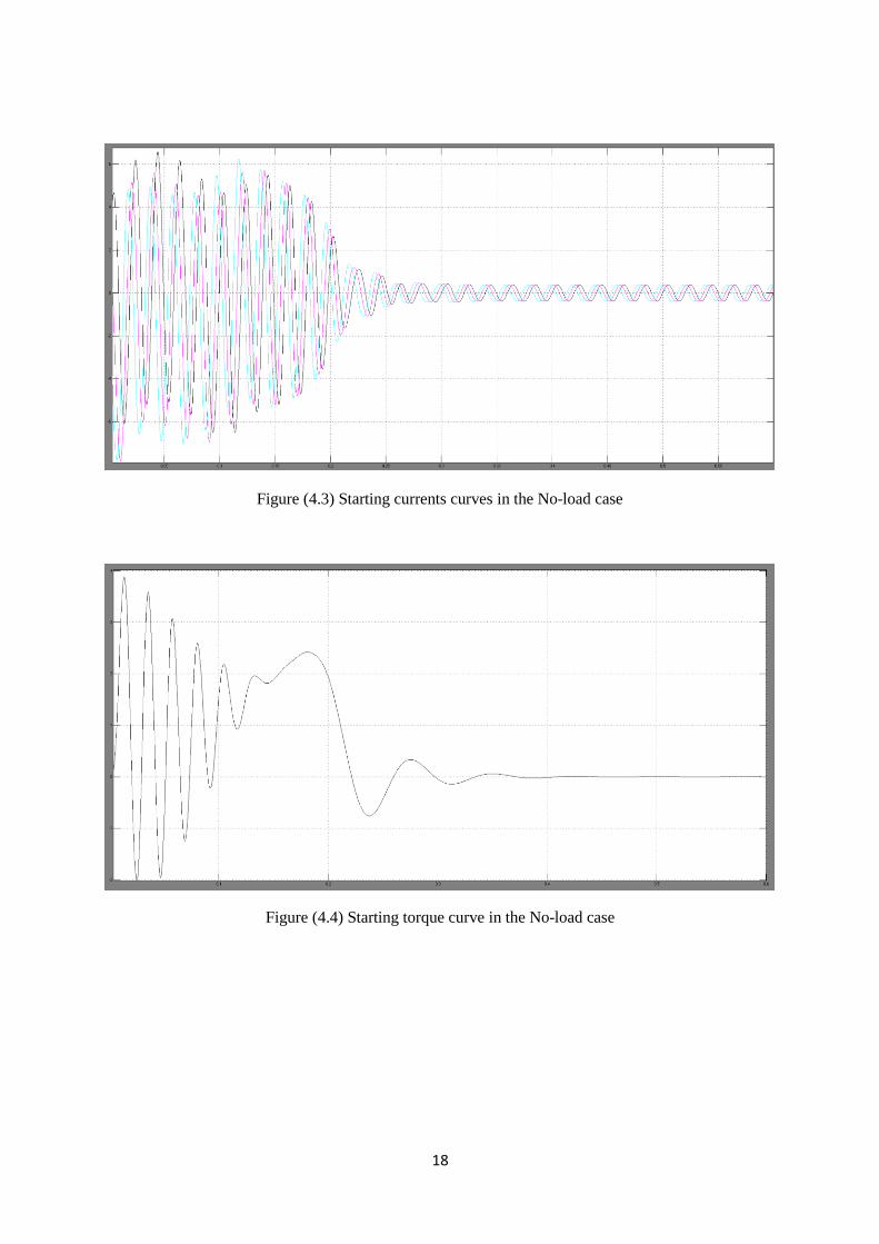
Figure (4.3) Starting currents curves in the No-load case
Figure (4.4) Starting torque curve in the No-load case
19
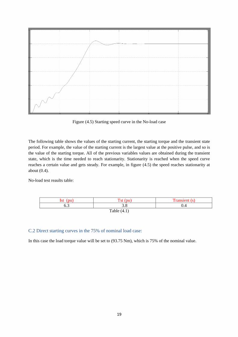
Figure (4.5) Starting speed curve in the No-load case
The following table shows the values of the starting current, the starting torque and the transient state
period. For example, the value of the starting current is the largest value at the positive pulse, and so is
the value of the starting torque. All of the previous variables values are obtained during the transient
state, which is the time needed to reach stationarity. Stationarity is reached when the speed curve
reaches a certain value and gets steady. For example, in figure (4.5) the speed reaches stationarity at
about (0.4).
No-load test reaults table:
Ist (pu) Tst (pu) Transient (s)
6.3 3.8 0.4
Table (4.1)
C.2 Direct starting curves in the 75% of nominal load case:
In this case the load torque value will be set to (93.75 Nm), which is 75% of the nominal value.
20
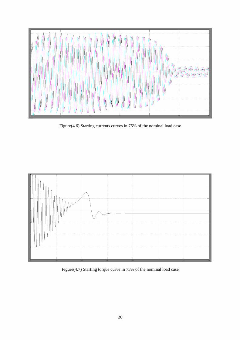
Figure(4.6) Starting currents curves in 75% of the nominal load case
Figure(4.7) Starting torque curve in 75% of the nominal load case
21
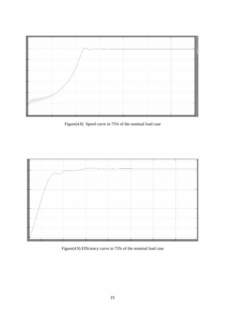
Figure(4.8) Speed curve in 75% of the nominal load case
Figure(4.9) Efficiency curve in 75% of the nominal load case
22
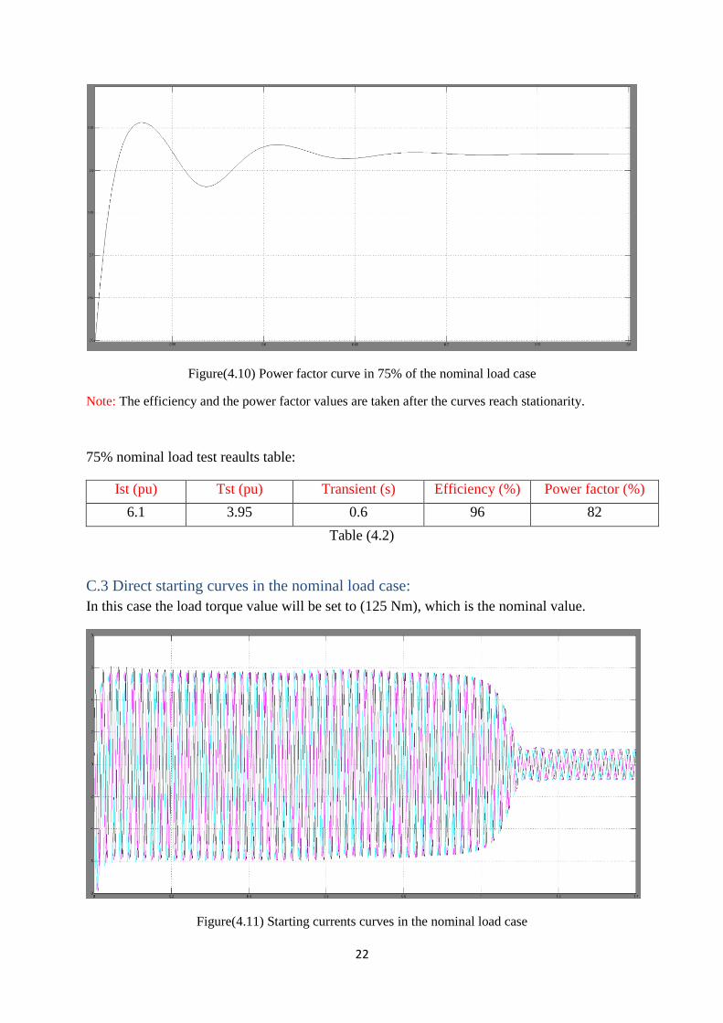
Figure(4.10) Power factor curve in 75% of the nominal load case
Note: The efficiency and the power factor values are taken after the curves reach stationarity.
75% nominal load test reaults table:
Ist (pu) Tst (pu) Transient (s) Efficiency (%) Power factor (%)
6.1 3.95 0.6 96 82
Table (4.2)
C.3 Direct starting curves in the nominal load case:
In this case the load torque value will be set to (125 Nm), which is the nominal value.
Figure(4.11) Starting currents curves in the nominal load case
23
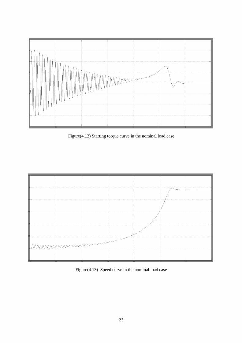
Figure(4.12) Starting torque curve in the nominal load case
Figure(4.13) Speed curve in the nominal load case
24
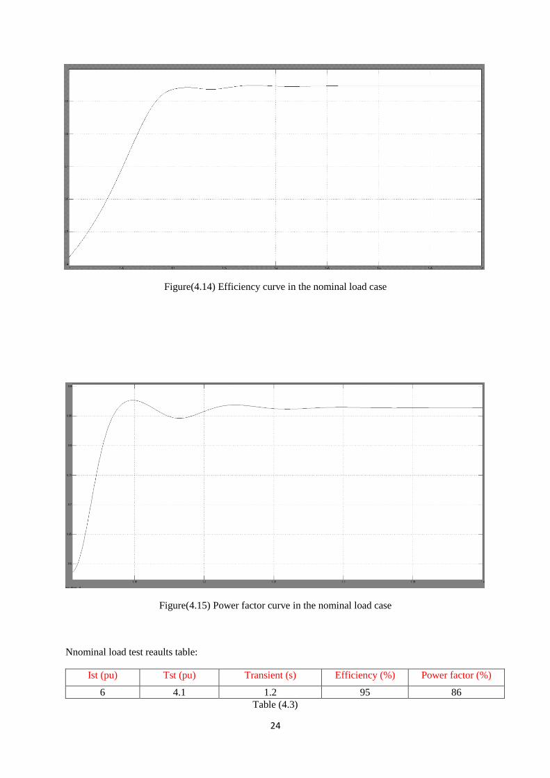
Figure(4.14) Efficiency curve in the nominal load case
Figure(4.15) Power factor curve in the nominal load case
Nnominal load test reaults table:
Ist (pu) Tst (pu) Transient (s) Efficiency (%) Power factor (%)
6 4.1 1.2 95 86
Table (4.3)
25
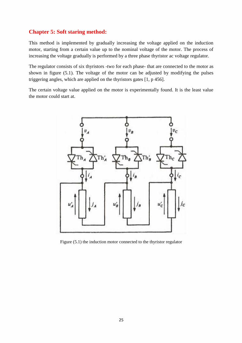
Chapter 5: Soft staring method:
This method is implemented by gradually increasing the voltage applied on the induction
motor, starting from a certain value up to the nominal voltage of the motor. The process of
increasing the voltage gradually is performed by a three phase thyristor ac voltage regulator.
The regulator consists of six thyristors -two for each phase- that are connected to the motor as
shown in figure (5.1). The voltage of the motor can be adjusted by modifying the pulses
triggering angles, which are applied on the thyristors gates [1, p 456].
The certain voltage value applied on the motor is experimentally found. It is the least value
the motor could start at.
Figure (5.1) the induction motor connected to the thyristor regulator
26
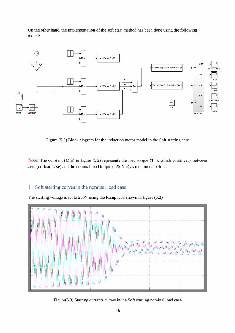
On the other hand, the implementation of the soft start method has been done using the following
model:
Figure (5.2) Block diagram for the induction motor model in the Soft starting case
Note: The constant (Mm) in figure (5.2) represents the load torque (Tm), which could vary between
zero (no-load case) and the nominal load torque (125 Nm) as mentioned before.
1. Soft starting curves in the nominal load case:
The starting voltage is set to 200V using the Ramp icon shown in figure (5.2)
Figure(5.3) Starting currents curves in the Soft starting nominal load case
27
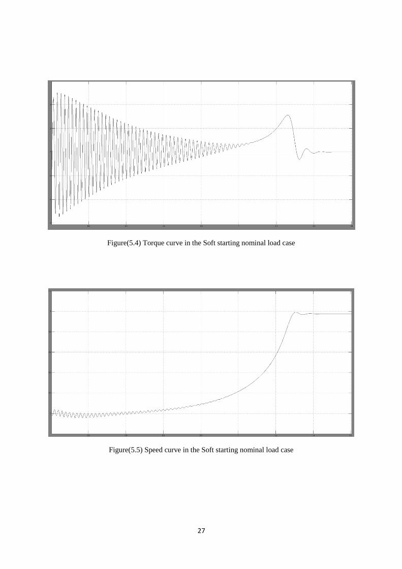
Figure(5.4) Torque curve in the Soft starting nominal load case
Figure(5.5) Speed curve in the Soft starting nominal load case
28
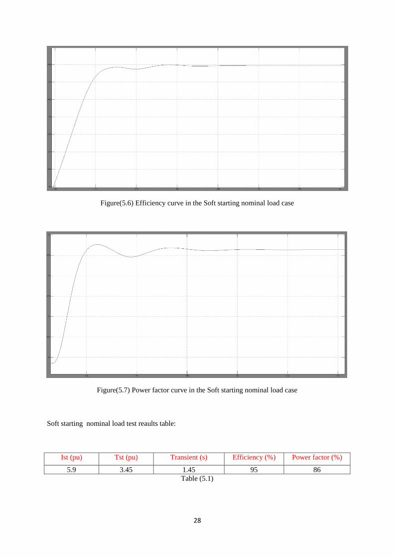
Figure(5.6) Efficiency curve in the Soft starting nominal load case
Figure(5.7) Power factor curve in the Soft starting nominal load case
Soft starting nominal load test reaults table:
Ist (pu) Tst (pu) Transient (s) Efficiency (%) Power factor (%)
5.9 3.45 1.45 95 86
Table (5.1)
29
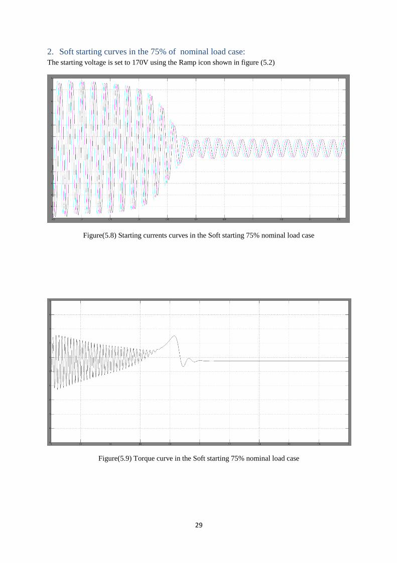
2. Soft starting curves in the 75% of nominal load case:
The starting voltage is set to 170V using the Ramp icon shown in figure (5.2)
Figure(5.8) Starting currents curves in the Soft starting 75% nominal load case
Figure(5.9) Torque curve in the Soft starting 75% nominal load case
30
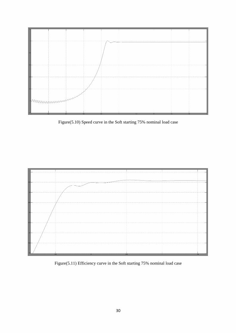
Figure(5.10) Speed curve in the Soft starting 75% nominal load case
Figure(5.11) Efficiency curve in the Soft starting 75% nominal load case
31
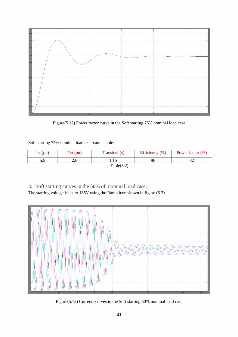
Figure(5.12) Power factor curve in the Soft starting 75% nominal load case
Soft starting 75% nominal load test reaults table:
Ist (pu) Tst (pu) Transient (s) Efficiency (%) Power factor (%)
5.8 2.6 1.15 96 82
Table(5.2)
3. Soft starting curves in the 50% of nominal load case:
The starting voltage is set to 135V using the Ramp icon shown in figure (5.2)
Figure(5.13) Currents curves in the Soft starting 50% nominal load case
32
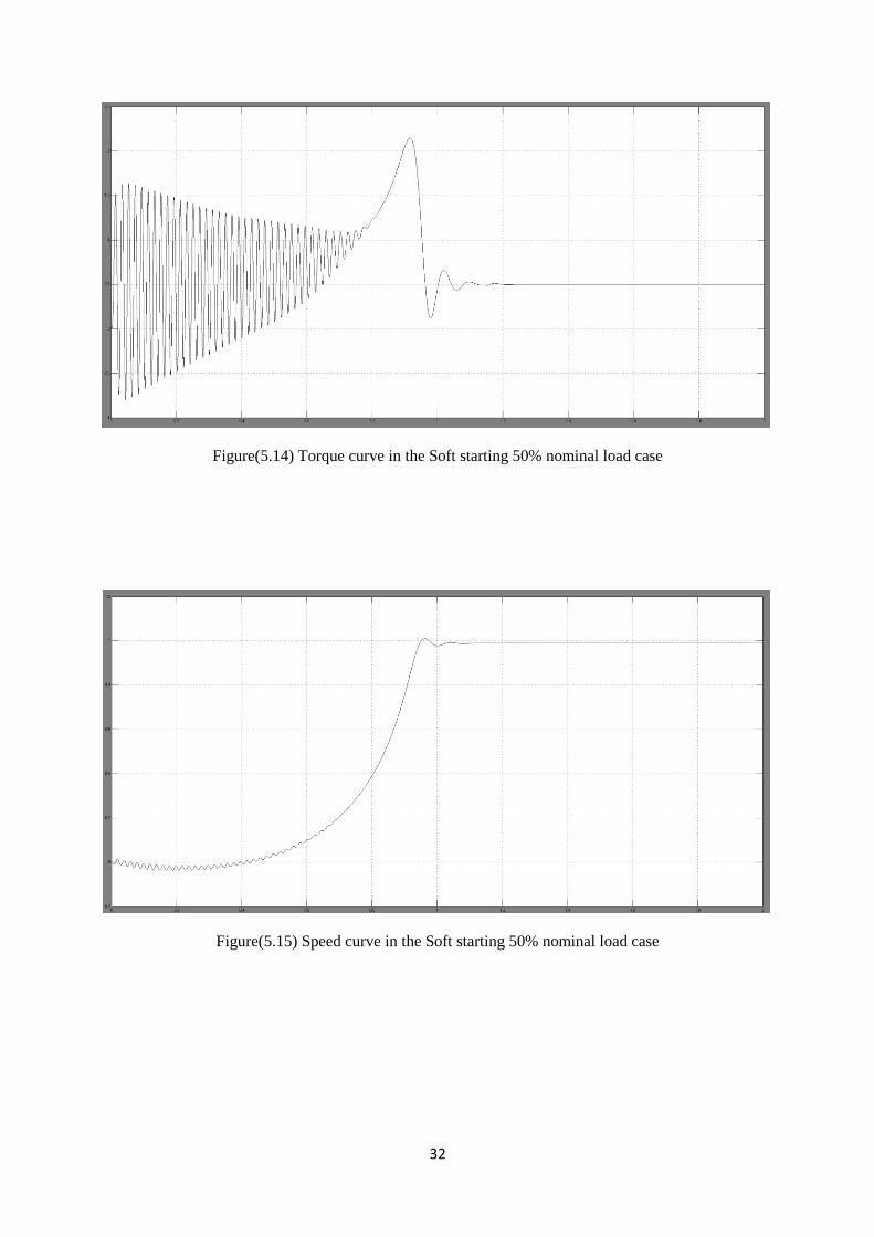
Figure(5.14) Torque curve in the Soft starting 50% nominal load case
Figure(5.15) Speed curve in the Soft starting 50% nominal load case
33
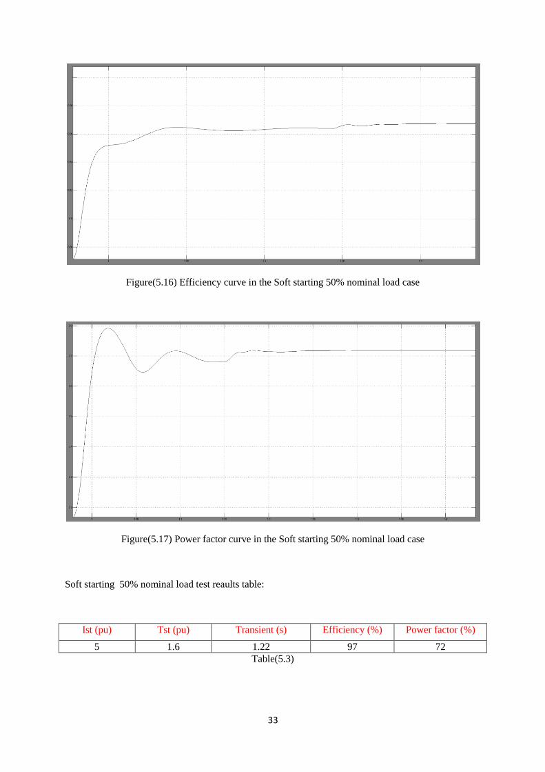
Figure(5.16) Efficiency curve in the Soft starting 50% nominal load case
Figure(5.17) Power factor curve in the Soft starting 50% nominal load case
Soft starting 50% nominal load test reaults table:
Ist (pu) Tst (pu) Transient (s) Efficiency (%) Power factor (%)
5 1.6 1.22 97 72
Table(5.3)
34
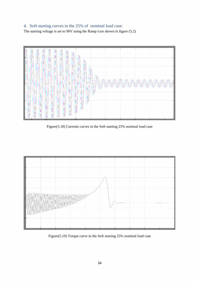
4. Soft starting curves in the 25% of nominal load case:
The starting voltage is set to 90V using the Ramp icon shown in figure (5.2)
Figure(5.18) Currents curves in the Soft starting 25% nominal load case
Figure(5.19) Torque curve in the Soft starting 25% nominal load case
35
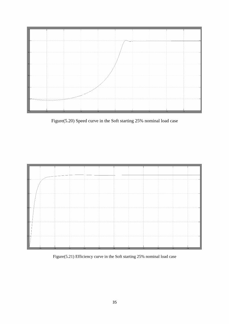
Figure(5.20) Speed curve in the Soft starting 25% nominal load case
Figure(5.21) Efficiency curve in the Soft starting 25% nominal load case
36
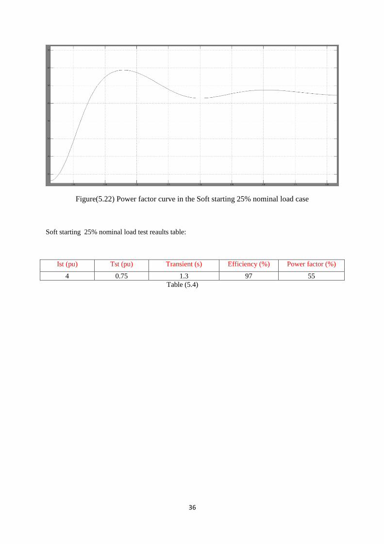
Figure(5.22) Power factor curve in the Soft starting 25% nominal load case
Soft starting 25% nominal load test reaults table:
Ist (pu) Tst (pu) Transient (s) Efficiency (%) Power factor (%)
4 0.75 1.3 97 55
Table (5.4)
37
Chapter 6: conclusions and discussion
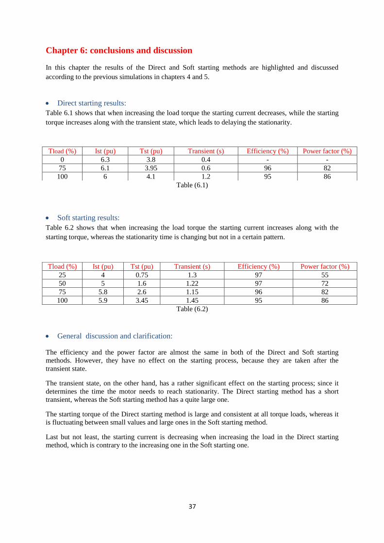
In this chapter the results of the Direct and Soft starting methods are highlighted and discussed
according to the previous simulations in chapters 4 and 5.
Direct starting results:
Table 6.1 shows that when increasing the load torque the starting current decreases, while the starting
torque increases along with the transient state, which leads to delaying the stationarity.
Table (6.1)
Soft starting results:
Table 6.2 shows that when increasing the load torque the starting current increases along with the
starting torque, whereas the stationarity time is changing but not in a certain pattern.
Table (6.2)
General discussion and clarification:
The efficiency and the power factor are almost the same in both of the Direct and Soft starting
methods. However, they have no effect on the starting process, because they are taken after the
transient state.
The transient state, on the other hand, has a rather significant effect on the starting process; since it
determines the time the motor needs to reach stationarity. The Direct starting method has a short
transient, whereas the Soft starting method has a quite large one.
The starting torque of the Direct starting method is large and consistent at all torque loads, whereas it
is fluctuating between small values and large ones in the Soft starting method.
Last but not least, the starting current is decreasing when increasing the load in the Direct starting
method, which is contrary to the increasing one in the Soft starting one.
Tload (%) Ist (pu) Tst (pu) Transient (s) Efficiency (%) Power factor (%)
0 6.3 3.8 0.4 - -
75 6.1 3.95 0.6 96 82
100 6 4.1 1.2 95 86
Tload (%) Ist (pu) Tst (pu) Transient (s) Efficiency (%) Power factor (%)
25 4 0.75 1.3 97 55
50 5 1.6 1.22 97 72
75 5.8 2.6 1.15 96 82
100 5.9 3.45 1.45 95 86

38
Conclusions:
The previous results showed that the Direct starting method requires a large starting current which
causes a disturbance to voltages on the supply lines. In other words, the large starting current produces
a severe voltage drop which affects the operation of other equipment. Other than that, it is a quite good
method because it provides a large starting torque in a short transient state, without the need of
external equipment to help starting the motor. The previous features make the Direct starting method
the most common one to start a 3ph induction motor.
The Soft starting method requires a reasonable starting current to generate a small starting torque at a
long transient state, not to mention the need of external thyristor voltage regulator which means extra
costs. On the other hand, it provides a smooth startup without any jerks along with a controlled
flawless acceleration. These features give the Soft starting method a reliable accuracy with less current
needed at the expense of stationarity delay and external equipment charges.

39
References:
[1] H. Boghos and A. Al Jazi, Asynchronous Machines. Damascus, Syria: DU, 2007.
[2] C. Ong, Dynamic Simulation of Electric Machinery. West Lafayette, Indiana: Upper Saddle River,
N.J. : Prentice Hall PTR, 1998
[3] Krause, P. C., ‘Simulation of symmetrical induction machinery’, IEEE T rans. Power Apparatus
Systems, Vol. PAS-84, No. 11, (1965)
[4] P. Stekl, 3-Phase AC Indudction Vector Control Drive with Single Shunt Current Sensing. Czech
Republic: Freescale Czech Systems Laboratories, 2007
[5] N. Mohan, Advanced electric drives analysis control and modeling using matlab / simulink.
Hoboken, New Jersey: John Wiley & Sons,Inc, 2014.
[6] http://publications.lib.chalmers.se/records/fulltext/64463/64463.pdf

40
Appendix 1
Notes: The simulations are not run by the m-file but are run by the Simulink models. However, the process
goes by these steps:
1. The m-file is opened and run, which stores the values at Matlab datasheet to be used when needed
in the Model.
2. Then the model is opened and run as well, and the parameters which are not defined in the model
are taken as values from the datasheet.
3. The main system in figure 3.2 has three inputs and five outputs, while the subsystem has only two
inputs and five outputs. The main system inputs are the three phase voltages implemented as
equations. The objective is to represent these voltages on Alpha Beta coordinates system as two
voltages, using simple conversion equations.
4. The subsystem -on the other hand - represents the equations found on pages (10, 11) as blocks, to
process and preview them as outputs. For instance, the current si can be easily substituted by a
simple integration and 3 gains (1/Ls, Rs/Ls, M/Ls), and then its value could be taken from the current
curves since each current has a unique color. The same method is used on all the blocks to produce the
outputs, which can be previewed by double clicking on the wanted icon in the main system.
5. If the reader would like to run the tests again he should make the changes (in the starting voltage for
example) in the model instead of the code since there is no code. This could be more difficult than the
standard way, but it is easier when making the simulations for the first time.
6. Regarding the current equations found on page 10, they are slightly different from the ones found in
reference number [5] since it has introduced the equations according to (qd) coordinates. Note that in
order to use [5] equations the axis (Alpha) should be considered as the axis (d) and the axis (Beta) as
(q). For instance, si corresponds to
s
di and si corresponds to
s
qi and so on.
Matlab simulation code
%DATA OF A THREE PHASE INDUCTION MOTOR
%Pn=18.5 kw;
M=0.0489; %H the constant of exchanged induction
Rr=0.16; %ohm the rotor resistance
Ls=0.05; %H the stator inductance
Lr=0.051; %H the rotor inductance
Rs=0.159; %ohm the stator resistance
P=2; % the number of pairs of poles
J=0.234%K.GM2 % moment of inertia
Wrb=314; % 2πf
Tb=125; % the nominal torque
Ib=52; % the nominal current
Tfactor1=((3/2)*M*P);
Tfactor2=(p/(J))
41
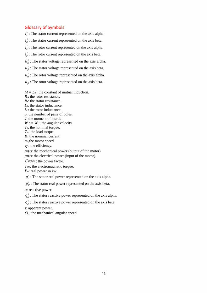
Glossary of Symbols si : The stator current represented on the axis alpha.
si : The stator current represented on the axis beta.
ri : The rotor current represented on the axis alpha.
ri : The rotor current represented on the axis beta.
su : The stator voltage represented on the axis alpha.
su : The stator voltage represented on the axis beta.
ru : The rotor voltage represented on the axis alpha.
ru : The rotor voltage represented on the axis beta.
M = Lm: the constant of mutual induction.
Rr: the rotor resistance.
Rs: the stator resistance.
Ls: the stator inductance.
Lr: the rotor inductance.
p: the number of pairs of poles.
J: the moment of inertia.
Wrb = Wr : the angular velocity.
Tb: the nominal torque.
Tm: the load torque.
Ib: the nominal current.
nb: the motor speed.
: the efficiency.
p2(t): the mechanical power (output of the motor).
p1(t): the electrical power (input of the motor).
1Cos : the power factor.
Tem: the electromagnetic torque.
Pn: real power in kw. sp : The stator real power represented on the axis alpha.
sp : The stator real power represented on the axis beta.
q: reactive power. sq : The stator reactive power represented on the axis alpha.
sq : The stator reactive power represented on the axis beta.
s: apparent power.
r :the mechanical angular speed.
42
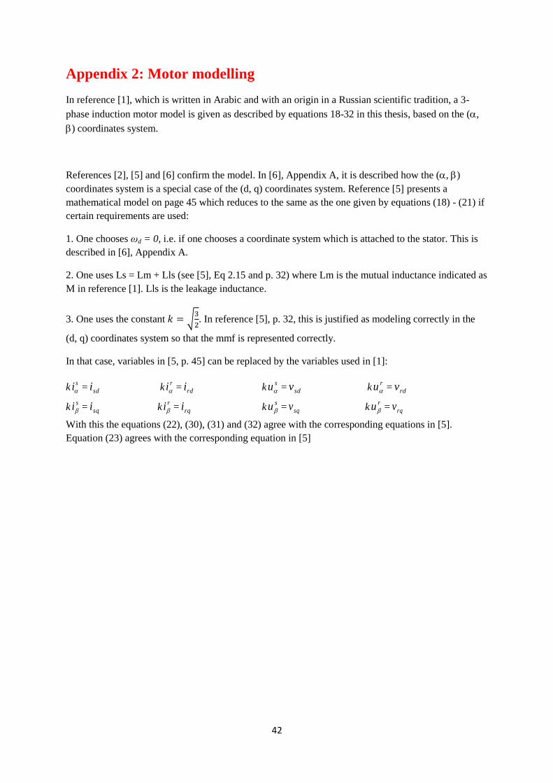
Appendix 2: Motor modelling
In reference [1], which is written in Arabic and with an origin in a Russian scientific tradition, a 3-
phase induction motor model is given as described by equations 18-32 in this thesis, based on the (,
) coordinates system.
References [2], [5] and [6] confirm the model. In [6], Appendix A, it is described how the (, )
coordinates system is a special case of the (d, q) coordinates system. Reference [5] presents a
mathematical model on page 45 which reduces to the same as the one given by equations (18) - (21) if
certain requirements are used:
1. One chooses ωd = 0, i.e. if one chooses a coordinate system which is attached to the stator. This is
described in [6], Appendix A.
2. One uses Ls = Lm + Lls (see [5], Eq 2.15 and p. 32) where Lm is the mutual inductance indicated as
M in reference [1]. Lls is the leakage inductance.
3. One uses the constant 𝑘 = √3
2. In reference [5], p. 32, this is justified as modeling correctly in the
(d, q) coordinates system so that the mmf is represented correctly.
In that case, variables in [5, p. 45] can be replaced by the variables used in [1]:
ksi = sdi k
ri = rdi ksu = sdv k
ru = rdv
ksi = sqi k
ri = rqi ksu = sqv k
ru = rqv
With this the equations (22), (30), (31) and (32) agree with the corresponding equations in [5].
Equation (23) agrees with the corresponding equation in [5]

43


![Ghid Selectie - Ups 3ph - [en]](https://img.pdfslide.us/doc/110x75/577cde091a28ab9e78ae432a/ghid-selectie-ups-3ph-en.jpg)