Embed Size (px)
Citation preview
Simulation approach in Matlab/Simulink forthe main components of a positioning unitin a closed-loop hydraulic circuit
BENJAMIN WOLFSetembro de 2016
“Simulation approach in Matlab/Simulink for the main
components of a positioning unit in a closed-loop
hydraulic circuit”
Master’s Thesis
by
Benjamin Wolf
born: 18th August 1987
in
Halle/Saale
Student Number: 1150120
Supervisor: Prof. Doutor Antonio Ferreira da Silva
Porto, December 2015 – September 2016

Statement of Authorship
I truthfully assure that I prepared this master’s thesis on my own independently. I quoted all
used tools completely and accurately and I marked everything what was taken unchanged or
with modifications from the work of others.
Porto, 26th September 16 …………………..…………………………….
(Benjamin Wolf)

Danksagung
Ich möchte meinen Eltern danken, die mich während meiner gesamten studentischen Aus-
bildung stets unterstützt haben, sowohl in moralischer wie auch finanzieller Hinsicht. Ohne
euch wäre das nicht möglich gewesen.
Ein besonderer Dank gilt meiner Freundin Susann. Du hast mich auch in schweren Zeiten
immer aufgerichtet und warst immer ein positiver Einfluss, der mir neue Kraft gegeben hat.
Table of Content
Formula Symbols .................................................................................................................... i
Abbreviations and Indices ..................................................................................................... iii
List of Figures ........................................................................................................................ iv
List of Tables ......................................................................................................................... vi
Abstract ................................................................................................................................. 1
1 Introduction .................................................................................................................... 2
2 Fundamentals ................................................................................................................ 4
2.1 Dynamic Behavior of Hydraulic Systems ................................................................. 4
2.2 Functionality of Proportional Valves ........................................................................ 6
2.3 Forced Oscillations of a Second Order System ....................................................... 8
2.4 Relationship between Time and Frequency Domain ...............................................13
3 Modelling of the Circuit ..................................................................................................20
4 Hydraulic Oil ..................................................................................................................21
5 Pipes .............................................................................................................................22
6 Cylinder .........................................................................................................................23
6.1 Theoretical Equations .............................................................................................23
6.2 Modelling with Simulink ..........................................................................................26
6.3 Results ...................................................................................................................28
7 Pressure Relief Valve ....................................................................................................29
7.1 Theoretical Considerations .....................................................................................29
7.2 Pressure Relief Valve Model with Matlab/Simulink .................................................33
7.3 Results ...................................................................................................................39
8 Proportional Directional Control Valve ...........................................................................41
8.1 Dynamic Model ......................................................................................................41
8.1.1 Signal Filtering ................................................................................................47
8.1.2 Finding Intersection .........................................................................................50
8.1.3 Determining Zero-Matrixes ..............................................................................53
8.1.4 Compute Amplitude and Phase Shift ...............................................................60
8.1.5 Optimization ....................................................................................................65
8.2 Static Model ...........................................................................................................71
8.3 Results ...................................................................................................................78
9 Summary and Discussion ..............................................................................................79
10 Recommendations for Future Work ...........................................................................82
11 Reference List............................................................................................................83
12 Appendix ....................................................................................................................85
12.1 Pipe Model .............................................................................................................85
12.2 Subsystems of Cylinder Model ...............................................................................86
12.3 Initializing Data for PRV .........................................................................................88
12.4 Simulink Model of Pressure Relief Valve ................................................................89
12.5 Measured Amplitude and Phase Data Points for 4WRSE-10 ..................................90
12.6 Measured Amplitude Data Points for KBSDG4V-3 Valve .......................................91
12.7 Simulink Model of Proportional Valve .....................................................................92
i
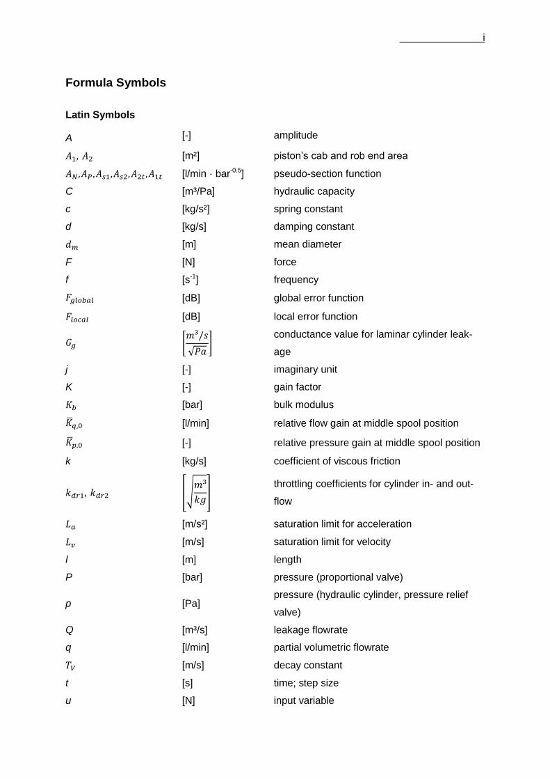
Formula Symbols
Latin Symbols
A [-] amplitude
𝐴1, 𝐴2 [m²] piston’s cab and rob end area
𝐴𝑁,𝐴𝑃,𝐴𝑠1,𝐴𝑠2,𝐴2𝑡,𝐴1𝑡 [l/min · bar-0.5] pseudo-section function
C [m³/Pa] hydraulic capacity
c [kg/s²] spring constant
d [kg/s] damping constant
𝑑𝑚 [m] mean diameter
F [N] force
f [s-1] frequency
𝐹𝑔𝑙𝑜𝑏𝑎𝑙 [dB] global error function
𝐹𝑙𝑜𝑐𝑎𝑙 [dB] local error function
𝐺𝑔 [𝑚³/𝑠
√𝑃𝑎]
conductance value for laminar cylinder leak-
age
j [-] imaginary unit
K [-] gain factor
𝐾𝑏 [bar] bulk modulus
�̅�𝑞,0 [l/min] relative flow gain at middle spool position
�̅�𝑝,0 [-] relative pressure gain at middle spool position
k [kg/s] coefficient of viscous friction
𝑘𝑑𝑟1, 𝑘𝑑𝑟2 [√𝑚³
𝑘𝑔]
throttling coefficients for cylinder in- and out-
flow
𝐿𝑎 [m/s²] saturation limit for acceleration
𝐿𝑣 [m/s] saturation limit for velocity
l [m] length
P [bar] pressure (proportional valve)
p [Pa] pressure (hydraulic cylinder, pressure relief
valve)
Q [m³/s] leakage flowrate
q [l/min] partial volumetric flowrate
𝑇𝑉 [m/s] decay constant
t [s] time; step size
u [N] input variable
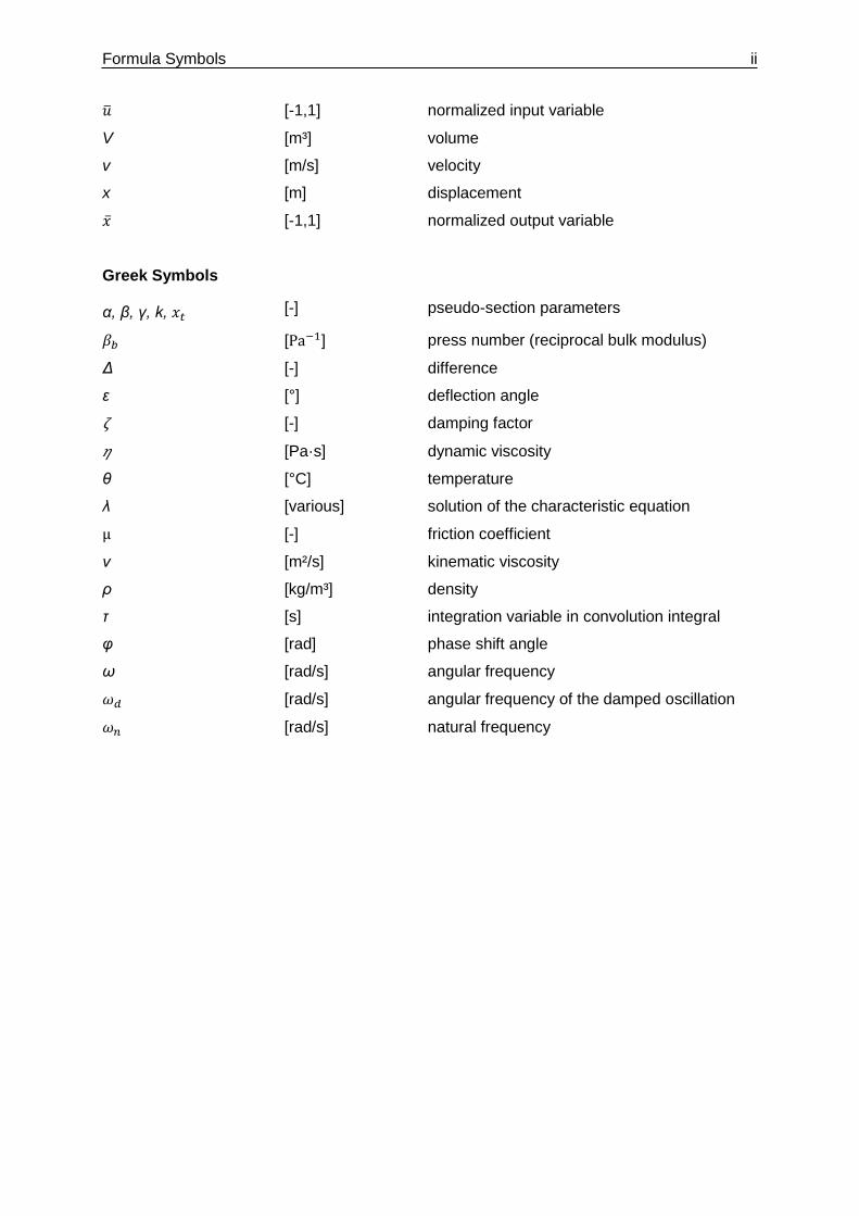
Formula Symbols ii
�̅� [-1,1] normalized input variable
V [m³] volume
v [m/s] velocity
x [m] displacement
�̅� [-1,1] normalized output variable
Greek Symbols
α, β, γ, k, 𝑥𝑡 [-] pseudo-section parameters
𝛽𝑏 [Pa−1] press number (reciprocal bulk modulus)
Δ [-] difference
ε [°] deflection angle
ζ [-] damping factor
𝜂 [Pa·s] dynamic viscosity
θ [°C] temperature
λ [various] solution of the characteristic equation
µ [-] friction coefficient
ν [m²/s] kinematic viscosity
ρ [kg/m³] density
τ [s] integration variable in convolution integral
φ [rad] phase shift angle
ω [rad/s] angular frequency
𝜔𝑑 [rad/s] angular frequency of the damped oscillation
𝜔𝑛 [rad/s] natural frequency
iii
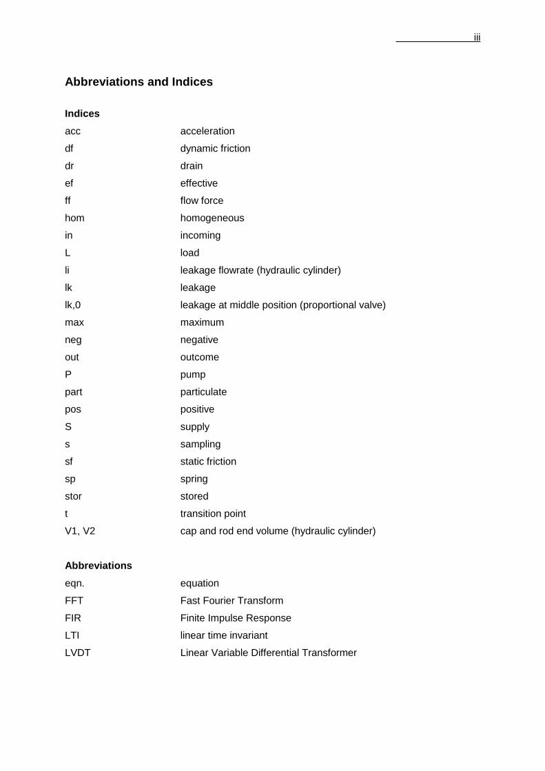
Abbreviations and Indices
Indices
acc acceleration
df dynamic friction
dr drain
ef effective
ff flow force
hom homogeneous
in incoming
L load
li leakage flowrate (hydraulic cylinder)
lk leakage
lk,0 leakage at middle position (proportional valve)
max maximum
neg negative
out outcome
P pump
part particulate
pos positive
S supply
s sampling
sf static friction
sp spring
stor stored
t transition point
V1, V2 cap and rod end volume (hydraulic cylinder)
Abbreviations
eqn. equation
FFT Fast Fourier Transform
FIR Finite Impulse Response
LTI linear time invariant
LVDT Linear Variable Differential Transformer
iv
List of Figures
Figure 2:1 Proportional Directional Valve Bosch Rexroth 4WRSE [5] .................................... 7
Figure 2:2 LVDT (1) [21] ........................................................................................................ 8
Figure 2:3 LVDT (2) [21] ........................................................................................................ 8
Figure 2:4 Spring-Mass-Damper System [20] ........................................................................ 8
Figure 2:5 Free Damped Oscillation .....................................................................................11
Figure 2:6 Superposition of natural and excitation frequency [7] ...........................................13
Figure 2:7 Spectrum of the Rectangle Function [9] ...............................................................14
Figure 2:8 Phase Shift in Complex Plane .............................................................................15
Figure 2:9 Convolution in time domain of LTI System [10] ....................................................16
Figure 2:10 Bode Diagram of Linear Second Order System .................................................17
Figure 2:11 Input and Output Signal for Different Excitation Frequencies .............................19
Figure 3:1 Hydraulic Circuit ..................................................................................................20
Figure 5:1 March of Pressure ...............................................................................................22
Figure 6:1 Cylinder Model ....................................................................................................23
Figure 6:2 Double Acting Cylinder Simulink Model ...............................................................27
Figure 6:3 Piston Displacement ............................................................................................28
Figure 7:1 Schematic Pressure relief Valve [2, p. 251] .........................................................29
Figure 7:2 Qualitative Pressure Relief Curves ......................................................................32
Figure 7:3 PRV Curves from Datasheet ...............................................................................32
Figure 7:4 Block Diagram PRV .............................................................................................33
Figure 7:5 Assembly Drawing Pressure Relief Valve [14] .....................................................33
Figure 7:6 Valve Catridge .....................................................................................................34
Figure 7:7 Dimensions Valve Housing ..................................................................................34
Figure 7:8 Spool Dimensions ................................................................................................35
Figure 7:9 Diameter Dimensions ..........................................................................................36
Figure 7:10 Limiting Velocity.................................................................................................38
Figure 7:11 PRV Pressure Response ...................................................................................39
Figure 7:12 PRV Displacement Response ...........................................................................39
Figure 7:13 PRV Drain Flow Response ................................................................................39
Figure 7:14 Real Static PRV Curve ......................................................................................40
Figure 7:15 General Static PRV Curve .................................................................................40
Figure 8:1 Amplitude and phase response curves [5] ...........................................................42
Figure 8:2 Linear Second Order Model .................................................................................43
Figure 8:3 Non-Linear Valve Model ......................................................................................43
Figure 8:4 Optimization of Dynamic Model ...........................................................................45
List of Figures v
Figure 8:5 Time and Frequency Domain (I) ..........................................................................48
Figure 8:6 Time and Frequency Domain (II) .........................................................................48
Figure 8:7 Filtering in Frequency Domain (II) ........................................................................49
Figure 8:8 Filtering in Frequency Domain (I) .........................................................................49
Figure 8:9 Filtered Signal in Time Domain (I) .......................................................................49
Figure 8:10 Filtered Signal in Time Domain (II).....................................................................49
Figure 8:11 Positive and Negative Intersections ...................................................................51
Figure 8:12 Computing Intersection Values ..........................................................................52
Figure 8:13 Flow Chart of Computing Signal Characteristic Arrays.......................................57
Figure 8:14 Flow Chart of Computing the Row Dimension ...................................................58
Figure 8:15 Flow Chart of Computing Zero Matrixes ............................................................59
Figure 8:16 Superposed Signal ............................................................................................60
Figure 8:17 Positive Matrix Array ..........................................................................................61
Figure 8:18 Negative Matrix Array ........................................................................................61
Figure 8:19 Checking for Steady-State Amplitude Behavior .................................................61
Figure 8:20 Non-Steady-State Oscillation (2) .......................................................................62
Figure 8:21 Non-Steady-State Oscillation (1) .......................................................................62
Figure 8:22 Computation of Phase Shift ...............................................................................63
Figure 8:23 Influence of Phase Shift .....................................................................................64
Figure 8:24 Optimization Results Linear System ..................................................................65
Figure 8:25 Determination of Velocity Saturation Parameters ...............................................66
Figure 8:26 Amplitude Response KBSDG4V-3 (I) ................................................................68
Figure 8:27 Amplitude Response KBSDG4V-3 (II) ...............................................................69
Figure 8:28 Amplitude Response 4WRSE-10 .......................................................................69
Figure 8:29 Pseudo-Section Function of Spool Position .......................................................72
Figure 8:30 Static Spool Position Model [17] ........................................................................73
Figure 8:31 Pressure Characteristic Curve ...........................................................................75
Figure 8:32 Flow Characteristic Curve ..................................................................................76
Figure 8:33 Leakage Flow ....................................................................................................76
Figure 8:34 Pseudo-Section Function of Valve 4WRSE-10 ..................................................78
Figure 12:1 Pipe Model ........................................................................................................85
vi
List of Tables
Table 2-1 Fluidic Energy Storages and State Variables [2, p. 121] ........................................ 5
Table 2-2 Block Diagram Notation [2, p. 120] ........................................................................ 6
Table 7-1 Valve Housing Dimensions (I) [14] ........................................................................35
Table 7-2 Valve Housing Dimensions (II) [14] .......................................................................35
Table 7-3 Spool Dimensions.................................................................................................35
Table 8-1 Sampling Frequency .............................................................................................47
Table 8-2 Signal Characteristic .............................................................................................54
Table 8-3 Column Dimension Case 1 ...................................................................................55
Table 8-4 Column Dimension Case 2 ...................................................................................55
Table 8-5 Column Dimension Case 3 ...................................................................................55
Table 8-6 Column Dimension Case 4 ...................................................................................56
Table 8-7 Optimization Results for Vickers Valve .................................................................67
Table 8-8 Initial Values for Optimization of 4WRSE-10 .........................................................70
1
Abstract
The replacement of on-off solenoids with solenoids which can adjust the spool position of a
directional valve proportionally to their input voltage was the groundwork for the development
of proportional valve technology. Due to their robustness and well-priced properties, propor-
tional valves are a good alternative to conventional servo-solenoid valves. Indeed, servo-
solenoid valves are highly precise but that makes them highly expensive as well. Additional-
ly, they place great demands on maintenance and industrial surroundings. Hence propor-
tional valves are widely-used in automation engineering. A common application is the posi-
tioning of actuators. Thus, a closed-loop circuit is necessary. In doing so, the proportional
valve’s input voltage is the manipulated value which enables a certain area for the oil to pass
through the valve. Therefore the flow rate to the actuator can be changed to control the actu-
ator position with high precision. In this thesis the main components of a hydraulic positioning
unit shall be modelled and simulated using the software Matlab/Simulink. That includes the
actuator, the pressure relief valve, connecting pipes and of course the proportional direction-
al control valve. With this model the positioning unit can be tested under different conditions
to make predictions on how the system is going to react.
Due to the fact that it was not possible to collect measured data from the several compo-
nents, measured data from the datasheets have been used to verify the models. For the ac-
tuator was no datasheet available. Consequently only a general model could be created. The
dynamic behavior of the pressure relief valve could be obtained by using the dimensions giv-
en in the datasheet. However, the datasheet does not provide any curves related to dynamic
behavior. Therefore only the static behavior was verifiable. The simulation of the proportional
directional control valve was divided into a static and a dynamic part. Based on flow, pres-
sure and leakage curves given by the manufacturer, pseudo-section functions have been
created. These functions characterize the relationship between normalized spool position
and flow rate. For simulating the dynamic behavior, a nonlinear Simulink model was created.
The model was fitted to nonlinear frequency response data points by using a Nelder-Mead
simplex optimization algorithm. Methodologies and models were subsequently tested with
used data from the manufacturer. The good quality of the results seems to support the ap-
proach. Nevertheless, the Simulink model has to be adjusted more properly to the measure-
ment curves.
All important components of a hydraulic positioning unit have been modelled. It is recom-
mended to make further improvements to adjust the Simulink model more properly to the
given curves in the datasheet. Subsequently, all components can be connected together to
implement the closed-loop circuit.
2
1 Introduction
Hydraulic positioning units are widely-used in technical applications. In general, the position-
ing unit consists of an actuator, a pressure relief valve, a proportional directional control
valve, connecting pipes and the pump. Due to the complex friction influence at the piston of a
hydraulic cylinder, the positioning unit has to be implemented as a closed-loop circuit. In this
thesis the named components of a hydraulic positioning unit shall be modelled and simulated
with Matlab/Simulink. A deeper understanding about the dynamic behavior for each compo-
nent is needed to be able to connect them and to develop an appropriate control law. There-
fore it is possible to make predictions about the system’s reaction under different conditions.
To describe the dynamic behavior of a technical system, it is important to determine its state
variables and energy storages. For this reason, typical energy storages and state variables
shall be determined with regard to hydraulic systems. Valves are used to control hydraulic
systems. Depending on their spool position they uncover a certain area the oil can pass
through. When the valve opens, a force acts on the spool. That can cause oscillations. Being
able to analyze the dynamic characteristics, forces oscillations of mechanical systems shall
be enlarged. Especially for proportional valves, manufacturers provide frequency response
curves in their datasheet to give information about the dynamic behavior. These amplitude
and phase ratio curves are given in frequency domain. Thus, the relationship of time and
frequency domain shall be discussed.
For the simulation of a hydraulic circuit, oil is an important factor. That’s why the most im-
portant properties of the oil shall be enlarged. Furthermore, it has to be discussed how they
can be computed and used in the simulation.
Finally, static and dynamic relations have to be found. Based on these relations models shall
be created and simulated in Matlab/Simulink. Subsequently, the results will be discussed.
In chapter 2, necessary fundamentals for are covered. It is discussed which energy storages
and state variables are common in hydraulic systems, how they can be identified from a sim-
plified in- and output model and why this is important for creating a dynamic simulation in
hydraulics. Furthermore the functionality of proportional directional control valves is ex-
plained. Their oscillation characteristics can be described with a damped second order sys-
tem which is also enlarged in this chapter. Due to the fact that valve manufacturers illustrate
the dynamical behavior with frequency response plots, the relationship between time and
frequency domain is discussed.
In chapter 3, the characteristics and functionality of the whole circuit is explained. It is de-
scribed which components exist in the circuit and how the work together.
Introduction 3
In chapter 4, all important parameters for developing an oil model are presented. Thereby it
is discussed which parameters can be assumed constant.
In chapter 5, the pipe system is modelled. The pipes connect all other main components to-
gether which makes them important for the circuit. The march of pressure is shown when oil
gets pumped into a pipe system with outlet.
In chapter 6, the hydraulic cylinder model is presented. It is shown how the cylinder can be
simplified and how energy storages, state variables, balance as well as static equations can
be determined from that. Furthermore, the simulation results are presented.
In chapter 7, the pressure relief valve is discussed. It is shown that the pressure relief valve
is simulated dynamically based on the given dimensions from the datasheet. As an alterna-
tive, a model is presented which describes the static relationship between pressure and flow
rate.
In chapter 8, the proportional directional control valve is simulated. It is explained why the
simulation had to split up into a dynamic and a static part. To simulate the dynamical behav-
ior, several functions were implemented in Matlab. Furthermore, it is shown how a Nelder-
Mead algorithm based optimizing function was used to find the best parameters for a non-
linear Simulink model which characterizes the valve behavior. The static valve behavior
when the spool is in fixed position is explained by the static model. Therefore it is shown how
the needed parameters can be obtained from the datasheet.
In chapter 9 and 10, the summary and conclusion is presented as well as the recommenda-
tions for the future work.
4
2 Fundamentals
2.1 Dynamic Behavior of Hydraulic Systems
A simulation is an important tool in modern technology and it is particularly used in engineer-
ing. What makes them so meaningful is the ability to reproduce a real system and make vir-
tual improvements to examine what the impact would be. The real system can be tested un-
der several conditions to make sure that it works appropriately for a particular application. An
immense advantage is that systems can be tested before being built without the strict need
of a prototype, which saves time and money. Furthermore, it allows the analysis of variant
model setups for the behavior of an individual parameter which clarifies its impact on the final
result. Simulations also allow observing the behavior of a system over a very short as well as
a very long period of time. Another important factor is that most real systems cannot be ana-
lyzed with adequate accuracy due to high complexity.
In this section, the five important steps of creating a simulation model shall be introduced in
relation to hydraulic systems. These are:
1) Drawing a schematic with all in- and output signals and coefficients
2) Identifying the energy storages and their state variables
3) Setting up balance equations
4) Complementing missing relations with static equations
5) Drawing a block diagram
As the first point makes clear, the starting step is drawing a schematic with all important sig-
nals coming in or going out of the system. In the context of hydraulics, pressures and flow
rates are the most common. The schematic provides a good view on the system and points
out why the dynamic system is accelerating.
In a second step, the energy storages of the system have to be identified. These indicate
where the dynamic system stores the energy contained in the system. A dynamic technical
system has one or more energy storages depending on the complexity. Storages can be di-
vided into concentrated and spatially distributed [1]. Dynamic systems with concentrated en-
ergy storages are represented by state variables which depend on time. Whereas spatially
distributed storages are described by state variables which depends on time and position.
Hence concentrated storages are used more often due to less complexity. The state varia-
bles are closely connected to the storages because they describe the amount of energy
which is contained in the systems storage elements [2, p. 120]. The state parameters are
also of high interest because they describe the dynamic behavior of the system and cannot
change abruptly. The following table gives an overview of all relevant energy storages used
in hydraulics.
Fundamentals 5
Table 2-1 Fluidic Energy Storages and State Variables [2, p. 121]
Process Type
of
Energy
Typical
Storage
State
Variable Energy
Function
of State
Variable
Mechanical
(translational)
Potential
Energy
spring constant
𝑐
(transl. spring)
dis-
placement 𝑥
1
2 𝑐 𝑥² 𝑥 = ∫ �̇�𝑑𝑡
Kinetic
Energy
mass
𝑚 velocity �̇�
1
2 𝑚 �̇�² �̇� =
1
𝑚∫𝐹𝑎𝑐𝑐𝑑𝑡
Mechanical
(rotational)
Potential
Energy
spring constant
𝑐𝑇
(rotat. spring)
angle 𝜑 1
2 𝑐𝑇 𝜑² 𝜑 = ∫𝜔𝑑𝑡
Kinetic
Energy
mass moment
of inertia J
angular fre-
quency 𝜔
1
2 𝐽 𝜔² 𝜔 =
1
𝐽∫𝑀𝑎𝑐𝑐𝑑𝑡
Fluidic
Pressure-
Volume-
Energy
capacity
𝐶𝑦 of a fluid
volume
pressure 𝑝 1
2𝐶𝑦 𝑝² 𝑝 =
1
𝐶𝑦∫𝑄𝑠𝑡𝑜𝑟𝑑𝑡
The last column in Table 2-1 illustrates the connection between state variables and the ener-
gy storages. A state variable is always proportional to the integral of certain input parame-
ters. These input parameters are the inputs for the integration blocks in the simulation and at
the same time they are part of balance equations. For this reason it is important to determine
the balance equations. Force and momentum balance equations on translational and rota-
tional masses as well as volume flow rate balances in capacities play a major role in hydrau-
lics. It is beneficial to bring them in a specific shape which is shown below.
𝐹𝑎𝑐𝑐 =∑𝐹𝑎𝑐𝑡𝑖𝑛𝑔 (2-1)
𝑀𝑎𝑐𝑐 =∑𝑀𝑎𝑐𝑡𝑖𝑛𝑔 (2-2)
𝐹𝑎𝑐𝑐 is the sum of all forces acting on the mass. That contains i.e. forces generated by pres-
sures, springs, friction or load. These forces can have positive or negative signs depending
on their direction. The same considerations can be applied to momentum balance eqn. (2-2).
Volumetric flow rate balance equations can be determined as following:
𝑄𝑠𝑡𝑜𝑟 =∑𝑄𝑖𝑛 − ∑𝑄𝑜𝑢𝑡 (2-3)
As eqn. (2-3) indicates, the stored volumetric flow rate is the difference between in- and out-
flowing oil from a certain capacity. From fluidic state variable computation (Table 2-1) can be
concluded that the pressure change 𝑑𝑝/𝑑𝑡 is proportional to 𝑄𝑠𝑡𝑜𝑟 when capacity is constant.
The fourth step is to complement missing relations with static equations to complete the
model. Static equations express the behavior for stabilized conditions. Finally, the block dia-
Fundamentals 6
gram can be drawn based on the shown equations. By the block diagram the simulation
model can be created with Matlab/Simulink.
Table 2-2 Block Diagram Notation [2, p. 120]
Name Function Block Diagram
Integration �̇�𝑜𝑢𝑡 = 𝑥𝑖𝑛; �̇�𝑜𝑢𝑡 = ∫𝑥𝑖𝑛𝑑𝑡
Linear statical
transfer element �̇�𝑜𝑢𝑡 = 𝐾𝑃 · 𝑥𝑖𝑛
Static non-linearity �̇�𝑜𝑢𝑡 = 𝑥𝑖𝑛1 · sin (𝑥𝑖𝑛2)
Balance equation �̇�𝑜𝑢𝑡 = 𝑥𝑖𝑛1 + 𝑥𝑖𝑛2 − 𝑥𝑖𝑛2
2.2 Functionality of Proportional Direction Control Valves
To master the general requirements of today’s hydraulic applications, valves are indispensa-
ble. Valves satisfy different tasks in hydraulics. The main function of hydraulic valves is to
regulate and control the magnitude of a hydraulic variable. This can be pressure or flow. Also
the circuit topology can be controlled by changing the fluid’s direction or by blocking it. That’s
why they are categorized in four different classes. These are pressure valves, flow valves,
directional valves and check valves [3, p. 110].
Pressure valves limit or restrict a certain pressure level respectively a pressure difference.
Flow-control valves spread or restrict the flow rate as required for the application. Directional
valves are used to control the direction of the flow rate. Check valves block the flow rate in
one or even both directions and repeal it under some specific circumstances. Each of these
four classes is also divided in many more sub types, which won’t be discussed further at this
point. The last valve group is the electrical operated hydraulic valves. These are directional
valves with the improvement of customized control electronics. The control electronics
makes sure that the spool can be adjusted continuously and with very high accuracy by an
input voltage or current. This characteristic is necessary to have when used in hydraulic con-
trol circuits as control element. The electrical operated valves can be divided into directional
servo valves and proportional valves. A torque motor is used to control the directional servo
valve’s spool position by having various amplifying stages. Generally it has two or three of
them to use very low input signals to control huge output signals. [4, p. 193]
Fundamentals 7
This type of valve is used in highly-precise applications and creates high demands on the
working environment. To get precision in the valve’s functionality, the manufacturing has to
be precise as well, what makes this type expensive. By contrast, proportional valves are ef-
fectively a further development of directional valves with simple switching solenoids. Propor-
tional valves are widely spread in automation engineering because of their robustness and
cheapness compared to servo valves. Due to the high precision it is possible when using
servo vales to achieve an adjustment of all four control edges around the working point at the
same time, whereas proportional valves adjust only one control edge. The others are either
closed or opened to ensure that the restricting effect doesn’t have an impact compared to the
relevant control edge. That allows higher manufacturing tolerances when producing the con-
trol edges. The proportional valve technology is used in proportional direction, pressure and
flow. However, when using proportional directional control valves it is necessary to have
stroke-controlled magnets which are able to adjust the spool position continuously without
any problems. Additionally, this permits to have the function of a flow control valve additional-
ly which is important to achieve a correct actuator position in position control applications. In
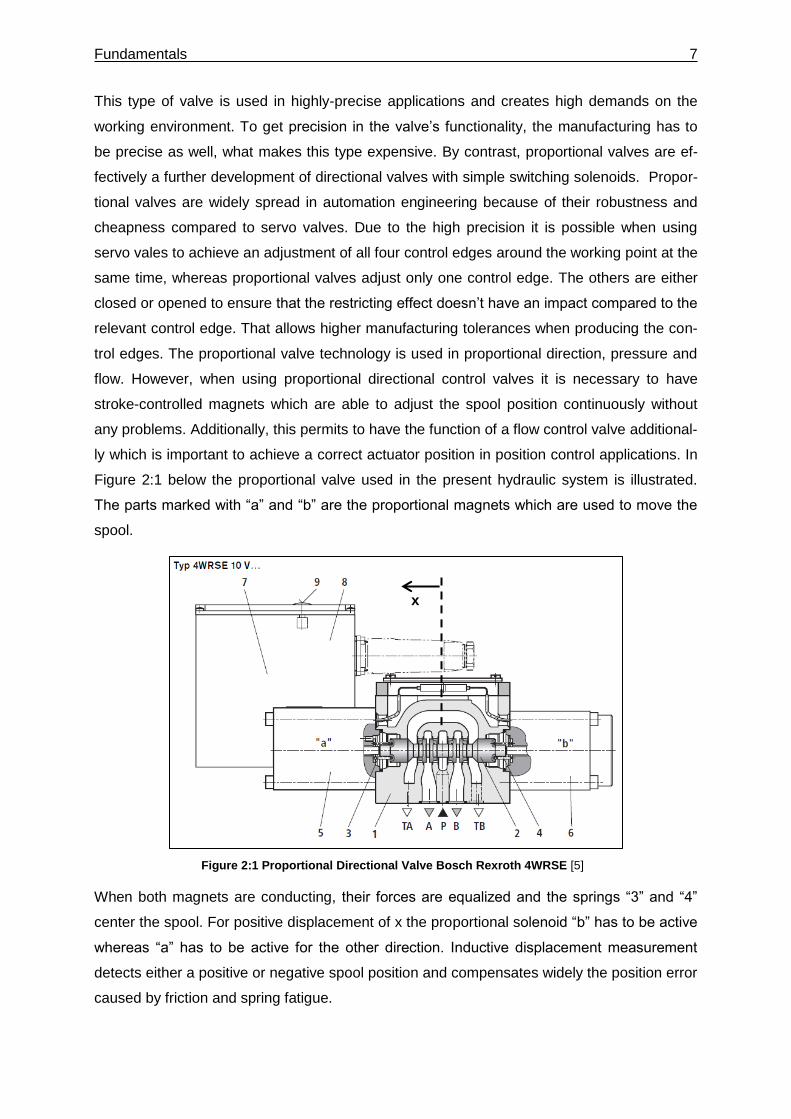
Figure 2:1 below the proportional valve used in the present hydraulic system is illustrated.
The parts marked with “a” and “b” are the proportional magnets which are used to move the
spool.
Figure 2:1 Proportional Directional Valve Bosch Rexroth 4WRSE [5]
When both magnets are conducting, their forces are equalized and the springs “3” and “4”
center the spool. For positive displacement of x the proportional solenoid “b” has to be active
whereas “a” has to be active for the other direction. Inductive displacement measurement
detects either a positive or negative spool position and compensates widely the position error
caused by friction and spring fatigue.
x
Fundamentals 8
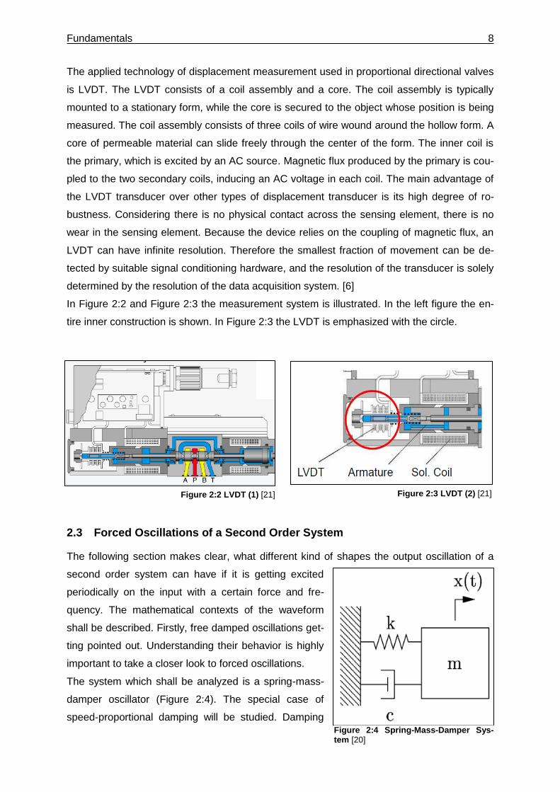
The applied technology of displacement measurement used in proportional directional valves
is LVDT. The LVDT consists of a coil assembly and a core. The coil assembly is typically
mounted to a stationary form, while the core is secured to the object whose position is being
measured. The coil assembly consists of three coils of wire wound around the hollow form. A
core of permeable material can slide freely through the center of the form. The inner coil is
the primary, which is excited by an AC source. Magnetic flux produced by the primary is cou-
pled to the two secondary coils, inducing an AC voltage in each coil. The main advantage of
the LVDT transducer over other types of displacement transducer is its high degree of ro-
bustness. Considering there is no physical contact across the sensing element, there is no
wear in the sensing element. Because the device relies on the coupling of magnetic flux, an
LVDT can have infinite resolution. Therefore the smallest fraction of movement can be de-
tected by suitable signal conditioning hardware, and the resolution of the transducer is solely
determined by the resolution of the data acquisition system. [6]
In Figure 2:2 and Figure 2:3 the measurement system is illustrated. In the left figure the en-
tire inner construction is shown. In Figure 2:3 the LVDT is emphasized with the circle.
2.3 Forced Oscillations of a Second Order System
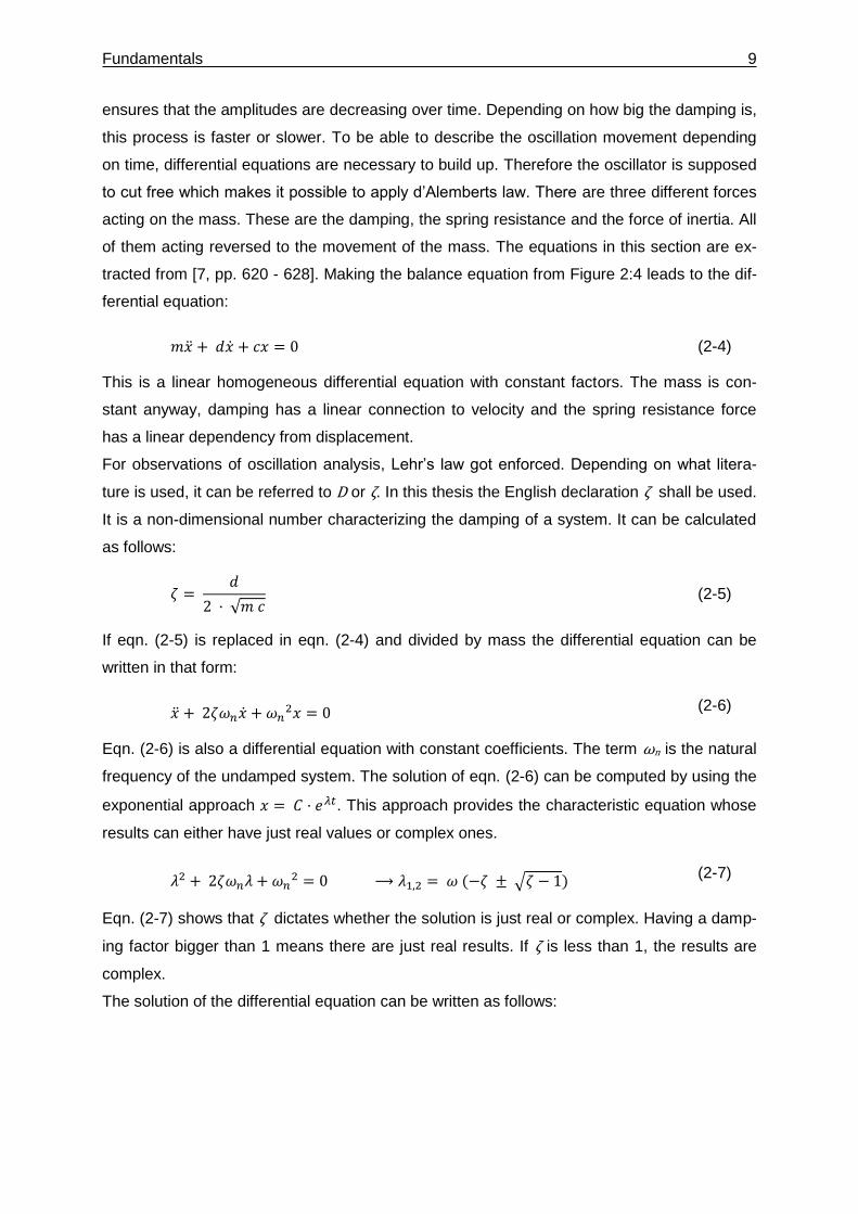
The following section makes clear, what different kind of shapes the output oscillation of a
second order system can have if it is getting excited
periodically on the input with a certain force and fre-
quency. The mathematical contexts of the waveform
shall be described. Firstly, free damped oscillations get-
ting pointed out. Understanding their behavior is highly
important to take a closer look to forced oscillations.
The system which shall be analyzed is a spring-mass-
damper oscillator (Figure 2:4). The special case of
speed-proportional damping will be studied. Damping
Figure 2:4 Spring-Mass-Damper Sys-tem [20]
Figure 2:3 LVDT (2) [21] Figure 2:2 LVDT (1) [21]
Fundamentals 9
ensures that the amplitudes are decreasing over time. Depending on how big the damping is,
this process is faster or slower. To be able to describe the oscillation movement depending
on time, differential equations are necessary to build up. Therefore the oscillator is supposed
to cut free which makes it possible to apply d’Alemberts law. There are three different forces
acting on the mass. These are the damping, the spring resistance and the force of inertia. All
of them acting reversed to the movement of the mass. The equations in this section are ex-
tracted from [7, pp. 620 - 628]. Making the balance equation from Figure 2:4 leads to the dif-
ferential equation:
𝑚�̈� + 𝑑�̇� + 𝑐𝑥 = 0 (2-4)
This is a linear homogeneous differential equation with constant factors. The mass is con-
stant anyway, damping has a linear connection to velocity and the spring resistance force
has a linear dependency from displacement.
For observations of oscillation analysis, Lehr’s law got enforced. Depending on what litera-
ture is used, it can be referred to D or ζ. In this thesis the English declaration ζ shall be used.
It is a non-dimensional number characterizing the damping of a system. It can be calculated
as follows:
𝜁 = 𝑑
2 · √𝑚 𝑐 (2-5)
If eqn. (2-5) is replaced in eqn. (2-4) and divided by mass the differential equation can be
written in that form:
�̈� + 2𝜁𝜔𝑛�̇� + 𝜔𝑛2𝑥 = 0 (2-6)
Eqn. (2-6) is also a differential equation with constant coefficients. The term ωn is the natural
frequency of the undamped system. The solution of eqn. (2-6) can be computed by using the
exponential approach 𝑥 = 𝐶 · 𝑒𝜆𝑡. This approach provides the characteristic equation whose
results can either have just real values or complex ones.
𝜆2 + 2𝜁𝜔𝑛𝜆 + 𝜔𝑛2 = 0 ⟶ 𝜆1,2 = 𝜔 (−𝜁 ± √𝜁 − 1)
(2-7)
Eqn. (2-7) shows that ζ dictates whether the solution is just real or complex. Having a damp-
ing factor bigger than 1 means there are just real results. If ζ is less than 1, the results are
complex.
The solution of the differential equation can be written as follows:
Fundamentals 10
𝑥 = 𝐶1𝑒𝜆1𝑡 + 𝐶2𝑒
𝜆2𝑡 = 𝑒−𝜁𝜔0𝑡 · (𝐶1𝑒𝜔𝑛√𝜁
2−1 𝑡 + 𝐶2𝑒𝜔𝑛√𝜁
2−1 𝑡) (2-8)
The factor before the brackets provides an asymptotic decay to zero. Having a damping fac-
tor of ζ = 1 results in a double solution with real values for λ. This case in particular is re-
ferred to a aperiodic limiting case. Under consideration of eqn. (2-8) follows:
𝑥 = 𝐶1𝑒𝜆𝑡 + 𝐶2𝑡 𝑒
𝜆𝑡 = 𝑒−𝜁𝜔0𝑡 · (𝐶1 + 𝐶2 𝑡) (2-9)
In this case the oscillation is dying out completely after half a period. Only in case ζ < 1 there
is going to be an oscillation at all. In boundaries of 0 < ζ < 1 exist a low damping which has
two conjugate-complex solutions for λ. Therefore Euler’s transformation is used:
𝑒𝑗𝑧 = cos(𝑧) + 𝑗 sin (𝑧) (2-10)
That means:
𝑥 = 𝐶1𝑒𝜆1𝑡 + 𝐶2𝑒
𝜆2𝑡
= 𝑒−𝜁𝜔𝑛𝑡 · (𝐶1𝑒𝜔𝑛 𝑗 √1 − 𝜁
2 𝑡 + 𝐶2𝑒−𝜔𝑛 𝑗 √1− 𝜁
2 𝑡) (2-11)
with:
𝜔𝑑 = ± 𝜔𝑛 √1 − 𝜁2
(2-12)
follows:
𝑥 = 𝑒−𝜁𝜔𝑛𝑡 · (𝐶1𝑒𝑗 𝜔𝑑 𝑡 + 𝐶2𝑒
−𝑗 𝜔𝑛 𝑡) (2-13)
= 𝑒−𝜁𝜔𝑛𝑡 · [𝐶1(cos (𝜔𝑑𝑡) + 𝑗 𝑠𝑖𝑛(𝜔𝑑𝑡) + 𝐶2(cos (𝜔𝑑𝑡) − 𝑗 𝑠𝑖𝑛(𝜔𝑑𝑡)] (2-14)
= 𝑒−𝜁𝜔𝑛𝑡 · [𝐴1(cos (𝜔𝑑𝑡) + 𝐴2 𝑠𝑖𝑛(𝜔𝑑𝑡)]
(2-15)
= 𝐶 · 𝑒−𝜁𝜔𝑛𝑡 · cos (𝜔𝑑𝑡 − 𝜑)
(2-16)
The qualitative characteristic for a free damped oscillation is illustrated in Figure 2:5 below.
Figure 2:5 acknowledges what also can already be read out from eqn. (2-16). The argument
of the cosine function characterizes the oscillation’s equation of motion depending on time.
This is forced to die out exponentially for t ⟶ ∞ with the increase of time due to term
𝐶 · 𝑒−𝜁𝜔𝑛𝑡. Thus, this term can be understood as envelopes of the function. These envelopes
are illustrated in the figure below as 𝑥𝑜 and 𝑥𝑢. These curves touch the function at those
points where the cosine function has their extreme values. However these points are not the
amplitudes of the damped function.
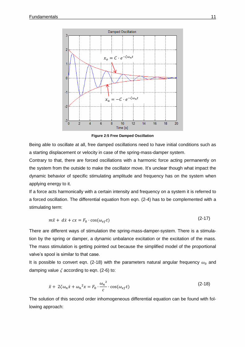
Fundamentals 11
Figure 2:5 Free Damped Oscillation
Being able to oscillate at all, free damped oscillations need to have initial conditions such as
a starting displacement or velocity in case of the spring-mass-damper system.
Contrary to that, there are forced oscillations with a harmonic force acting permanently on
the system from the outside to make the oscillator move. It’s unclear though what impact the
dynamic behavior of specific stimulating amplitude and frequency has on the system when
applying energy to it.
If a force acts harmonically with a certain intensity and frequency on a system it is referred to
a forced oscillation. The differential equation from eqn. (2-4) has to be complemented with a
stimulating term:
𝑚�̈� + 𝑑�̇� + 𝑐𝑥 = 𝐹0 · cos (𝜔𝑒𝑓𝑡) (2-17)
There are different ways of stimulation the spring-mass-damper-system. There is a stimula-
tion by the spring or damper, a dynamic unbalance excitation or the excitation of the mass.
The mass stimulation is getting pointed out because the simplified model of the proportional
valve’s spool is similar to that case.
It is possible to convert eqn. (2-18) with the parameters natural angular frequency 𝜔0 and
damping value ζ according to eqn. (2-6) to:
�̈� + 2𝜁𝜔𝑛�̇� + 𝜔𝑛2𝑥 = 𝐹0 ·
𝜔𝑛²
𝑐· cos (𝜔𝑒𝑓𝑡)
(2-18)
The solution of this second order inhomogeneous differential equation can be found with fol-
lowing approach:
𝑥𝑜 = 𝐶 · 𝑒−𝜁𝜔𝑛𝑡
𝑥𝑢 = −𝐶 · 𝑒−𝜁𝜔𝑛𝑡
Fundamentals 12
𝑥 = 𝑥ℎ𝑜𝑚 + 𝑥𝑝𝑎𝑟𝑡 (2-19)
Therefore the solution of the homogeneous term can be copied from eqn. (2-16) due to the
fact that there is no change in the systems setup. But the particulate solution which only re-
fers to excitation term has to be found as well. The following approach can be applied:
𝑥𝑝𝑎𝑟𝑡 = 𝐴 cos (𝜔𝑒𝑓𝑡 − 𝜑) (2-20)
and replaced into eqn.(2-18):
(−
𝐹0𝜔𝑛2
𝑐⁄ − 𝐴 𝜔𝑒𝑓2 cos(𝜑) + 2𝐴𝜁𝜔𝑛𝜔𝑒𝑓 sin(𝜑) + 𝐴 𝜔𝑛
2 cos(𝜑)) 𝑐𝑜𝑠(𝜔𝑒𝑓𝑡)
+ (−𝐴 𝜔𝑒𝑓2 sin(𝜑) + 2𝐴𝜁𝜔𝑛𝜔𝑒𝑓 cos(𝜑) + 𝐴 𝜔𝑛
2 sin(𝜑))𝑠𝑖𝑛(𝜔𝑒𝑓𝑡) = 0
(2-21)
Eqn. (2-21) is just able to be zero for any value of t if both brackets on the left side get set
zero. Therefore, both brackets getting set to zero. Doing so for the second bracket results in
the following calculation for φ:
𝑡𝑎𝑛(𝜑) = 2𝜁𝜔𝑛𝜔𝑒𝑓
𝜔𝑛2 −𝜔𝑒𝑓
2⁄ = 2𝜁 (
𝜔𝑒𝑓𝜔𝑛
)
1 − (𝜔𝑒𝑓𝜔𝑛
) ²⁄
(2-22)
Setting the first bracket to zero leads after some conversions to the last missing value of A:
𝐴 =
𝐹0𝑐
√[1 − (𝜔𝑒𝑓𝜔𝑛
) ²] + 4𝜁² (𝜔𝑒𝑓𝜔𝑛
) ²⁄ (2-23)
With eqn. (2-22) and eqn. (2-23) the solution of the particulate part is complete. Hence, the
general solution of the oscillation’s differential equation can be described. By looking at the
homogeneous and inhomogeneous part of the solution it can be determined that both of
them include a cosine function. That’s why the overall solution can be understood as a inter-
fering of two oscillations. According to eqn. (2-19), the final function is as follows:
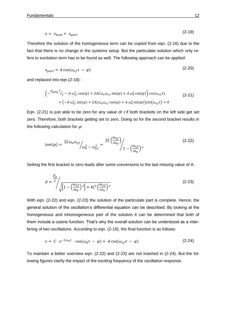
𝑥 = 𝐶 · 𝑒−𝜁𝜔𝑛𝑡 · cos (𝜔𝑑𝑡 − 𝜑) + 𝐴 cos (𝜔𝑒𝑓𝑡 − 𝜑) (2-24)
To maintain a better overview eqn. (2-22) and (2-23) are not inserted in (2-24). But the fol-
lowing figures clarify the impact of the exciting frequency of the oscillation response.
Fundamentals 13
Figure 2:6 Superposition of natural and excitation frequency [7]
Figure 2:6 clarifies that depending on the excitation frequency the output oscillation has a
different shape. Due to the negative exponential function, the natural frequency dies out. Af-
terwards the system oscillates just with the excitation frequency.
2.4 Relationship between Time and Frequency Domain
Manufactures normally announce the behavior of proportional valves by illustrating the Bode
diagram in their data sheets. A Bode diagram helps to understand how the valve behaves in
terms of phase and amplitude at a certain frequency. This section shall show why this is
necessary to know in order to examine the valve’s behavior in the time domain.
Basically, the Bode diagram consists of two different plots which is on the one hand ampli-
tude ratio over frequency and on the other hand phase shift over frequency. In contrast to
that, dynamic simulations are related to the time domain what brings out the necessity of
converting one into the other to be able to extract the information needed. Therefore, the
Fourier transform shall be introduced.
If an input is getting supplied to a system this signal can be transformed to frequency domain
using the Fourier transform. Hence eqn. (2-25) shows the forward Fourier transform whereas
(2-26) shows the inverse.
Fundamentals 14
𝑠(𝑡) ⊶ 𝑆(𝑓) = ∫ 𝑠(𝑡) · 𝑒−𝑗2𝜋𝑓𝑡+∞
−∞
𝑑𝑡 (2-25) [8]
𝑆(𝑓) ⊶ 𝑠(𝑡) = ∫ 𝑠(𝑡) · 𝑒−𝑗2𝜋𝑓𝑡+∞
−∞
𝑑𝑡 (2-26) [8]
Doing that is possible due to the fact that every periodical function respectively signal can be
reconstructed with a sum of sinusoids added up one after another. That allows looking at a
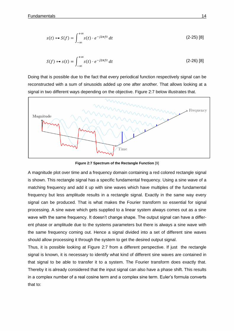
signal in two different ways depending on the objective. Figure 2:7 below illustrates that.
Figure 2:7 Spectrum of the Rectangle Function [9]
A magnitude plot over time and a frequency domain containing a red colored rectangle signal
is shown. This rectangle signal has a specific fundamental frequency. Using a sine wave of a
matching frequency and add it up with sine waves which have multiples of the fundamental
frequency but less amplitude results in a rectangle signal. Exactly in the same way every
signal can be produced. That is what makes the Fourier transform so essential for signal
processing. A sine wave which gets supplied to a linear system always comes out as a sine
wave with the same frequency. It doesn’t change shape. The output signal can have a differ-
ent phase or amplitude due to the systems parameters but there is always a sine wave with
the same frequency coming out. Hence a signal divided into a set of different sine waves
should allow processing it through the system to get the desired output signal.
Thus, it is possible looking at Figure 2:7 from a different perspective. If just the rectangle
signal is known, it is necessary to identify what kind of different sine waves are contained in
that signal to be able to transfer it to a system. The Fourier transform does exactly that.
Thereby it is already considered that the input signal can also have a phase shift. This results
in a complex number of a real cosine term and a complex sine term. Euler’s formula converts
that to:
Fundamentals 15
𝑒𝑗𝑡 = cos(𝑡) + 𝑗 𝑠𝑖𝑛(𝑡) (2-27) [10]
Using this form makes it easier to compute the complex number. This is already included in
eqn. (2-25) and (2-26) as it is shown above.
Figure 2:8 below shows the relationship between phase shift and the assumption of a com-
plex number.
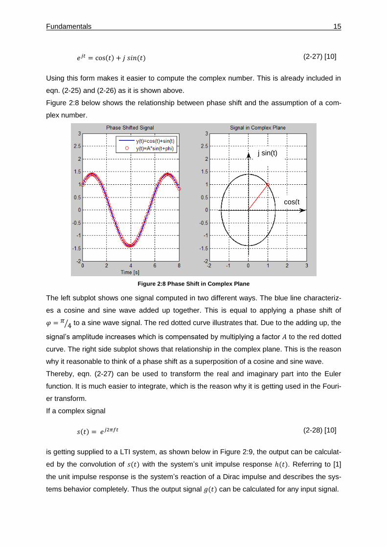
Figure 2:8 Phase Shift in Complex Plane
The left subplot shows one signal computed in two different ways. The blue line characteriz-
es a cosine and sine wave added up together. This is equal to applying a phase shift of
𝜑 = 𝜋 4⁄ to a sine wave signal. The red dotted curve illustrates that. Due to the adding up, the
signal’s amplitude increases which is compensated by multiplying a factor 𝐴 to the red dotted
curve. The right side subplot shows that relationship in the complex plane. This is the reason
why it reasonable to think of a phase shift as a superposition of a cosine and sine wave.
Thereby, eqn. (2-27) can be used to transform the real and imaginary part into the Euler
function. It is much easier to integrate, which is the reason why it is getting used in the Fouri-
er transform.
If a complex signal
𝑠(𝑡) = 𝑒𝑗2𝜋𝑓𝑡 (2-28) [10]
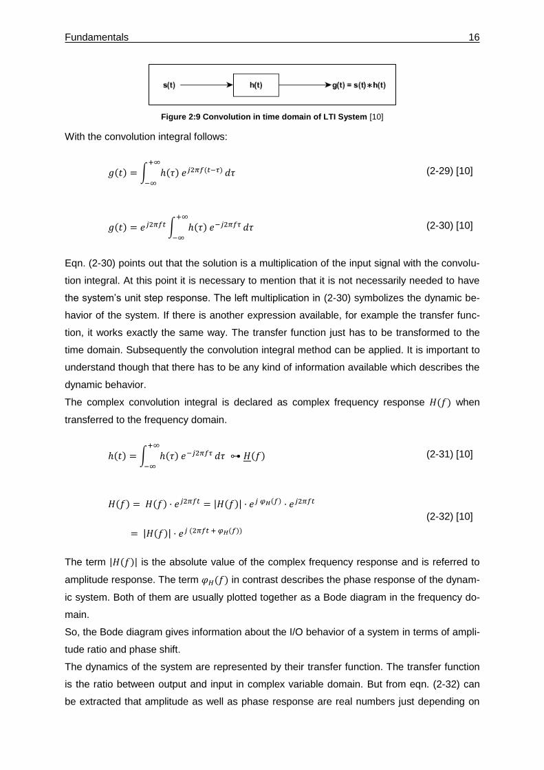
is getting supplied to a LTI system, as shown below in Figure 2:9, the output can be calculat-
ed by the convolution of 𝑠(𝑡) with the system’s unit impulse response ℎ(𝑡). Referring to [1]
the unit impulse response is the system’s reaction of a Dirac impulse and describes the sys-
tems behavior completely. Thus the output signal 𝑔(𝑡) can be calculated for any input signal.
j sin(t)
cos(t
)
Fundamentals 16
Figure 2:9 Convolution in time domain of LTI System [10]
With the convolution integral follows:
𝑔(𝑡) = ∫ ℎ(𝜏) 𝑒𝑗2𝜋𝑓(𝑡−𝜏)+∞
−∞
𝑑𝜏 (2-29) [10]
𝑔(𝑡) = 𝑒𝑗2𝜋𝑓𝑡∫ ℎ(𝜏) 𝑒−𝑗2𝜋𝑓𝜏+∞
−∞
𝑑𝜏 (2-30) [10]
Eqn. (2-30) points out that the solution is a multiplication of the input signal with the convolu-
tion integral. At this point it is necessary to mention that it is not necessarily needed to have
the system’s unit step response. The left multiplication in (2-30) symbolizes the dynamic be-
havior of the system. If there is another expression available, for example the transfer func-
tion, it works exactly the same way. The transfer function just has to be transformed to the
time domain. Subsequently the convolution integral method can be applied. It is important to
understand though that there has to be any kind of information available which describes the
dynamic behavior.
The complex convolution integral is declared as complex frequency response 𝐻(𝑓) when
transferred to the frequency domain.
ℎ(𝑡) = ∫ ℎ(𝜏) 𝑒−𝑗2𝜋𝑓𝜏+∞
−∞
𝑑𝜏 ⊶ 𝐻(𝑓) (2-31) [10]
𝐻(𝑓) = 𝐻(𝑓) · 𝑒𝑗2𝜋𝑓𝑡 = |𝐻(𝑓)| · 𝑒𝑗 𝜑𝐻(𝑓) · 𝑒𝑗2𝜋𝑓𝑡
= |𝐻(𝑓)| · 𝑒𝑗 (2𝜋𝑓𝑡 + 𝜑𝐻(𝑓))
(2-32) [10]
The term |𝐻(𝑓)| is the absolute value of the complex frequency response and is referred to
amplitude response. The term 𝜑𝐻(𝑓) in contrast describes the phase response of the dynam-
ic system. Both of them are usually plotted together as a Bode diagram in the frequency do-
main.
So, the Bode diagram gives information about the I/O behavior of a system in terms of ampli-
tude ratio and phase shift.
The dynamics of the system are represented by their transfer function. The transfer function
is the ratio between output and input in complex variable domain. But from eqn. (2-32) can
be extracted that amplitude as well as phase response are real numbers just depending on
Fundamentals 17
the frequency which gets supplied to the system. For further explanations, Figure 2:10 shall
be introduced.
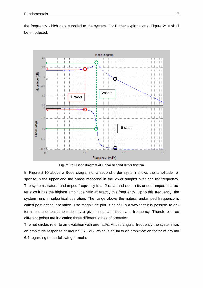
Figure 2:10 Bode Diagram of Linear Second Order System
In Figure 2:10 above a Bode diagram of a second order system shows the amplitude re-
sponse in the upper and the phase response in the lower subplot over angular frequency.
The systems natural undamped frequency is at 2 rad/s and due to its underdamped charac-
teristics it has the highest amplitude ratio at exactly this frequency. Up to this frequency, the
system runs in subcritical operation. The range above the natural undamped frequency is
called post-critical operation. The magnitude plot is helpful in a way that it is possible to de-
termine the output amplitudes by a given input amplitude and frequency. Therefore three
different points are indicating three different states of operation.
The red circles refer to an excitation with one rad/s. At this angular frequency the system has
an amplitude response of around 16.5 dB, which is equal to an amplification factor of around
6.4 regarding to the following formula:
1 rad/s
6 rad/s
2rad/s
Fundamentals 18
𝐴[𝑑𝐵] = 20 · 𝑙𝑜𝑔10 (𝐴𝑜𝑢𝑡𝑝𝑢𝑡𝐴𝑖𝑛𝑝𝑢𝑡
) (2-33)
Thus it appears that if this system is getting excited by a force, acting periodically with 1 rad/s
on the system, the input amplitude is getting increased by factor 6.4. Following the red
dashed line, a phase response of -6° can be read out. These observations are valid for
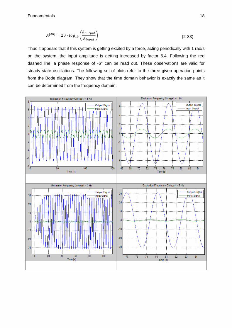
steady state oscillations. The following set of plots refer to the three given operation points
from the Bode diagram. They show that the time domain behavior is exactly the same as it
can be determined from the frequency domain.
Fundamentals 19
Figure 2:11 Input and Output Signal for Different Excitation Frequencies
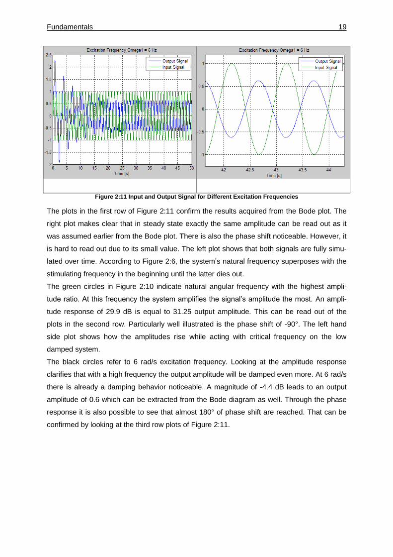
The plots in the first row of Figure 2:11 confirm the results acquired from the Bode plot. The
right plot makes clear that in steady state exactly the same amplitude can be read out as it
was assumed earlier from the Bode plot. There is also the phase shift noticeable. However, it
is hard to read out due to its small value. The left plot shows that both signals are fully simu-
lated over time. According to Figure 2:6, the system’s natural frequency superposes with the
stimulating frequency in the beginning until the latter dies out.
The green circles in Figure 2:10 indicate natural angular frequency with the highest ampli-
tude ratio. At this frequency the system amplifies the signal’s amplitude the most. An ampli-
tude response of 29.9 dB is equal to 31.25 output amplitude. This can be read out of the
plots in the second row. Particularly well illustrated is the phase shift of -90°. The left hand
side plot shows how the amplitudes rise while acting with critical frequency on the low
damped system.
The black circles refer to 6 rad/s excitation frequency. Looking at the amplitude response
clarifies that with a high frequency the output amplitude will be damped even more. At 6 rad/s
there is already a damping behavior noticeable. A magnitude of -4.4 dB leads to an output
amplitude of 0.6 which can be extracted from the Bode diagram as well. Through the phase
response it is also possible to see that almost 180° of phase shift are reached. That can be
confirmed by looking at the third row plots of Figure 2:11.
20
3 Modelling of the Circuit
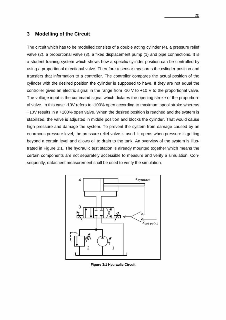
The circuit which has to be modelled consists of a double acting cylinder (4), a pressure relief
valve (2), a proportional valve (3), a fixed displacement pump (1) and pipe connections. It is
a student training system which shows how a specific cylinder position can be controlled by
using a proportional directional valve. Therefore a sensor measures the cylinder position and
transfers that information to a controller. The controller compares the actual position of the
cylinder with the desired position the cylinder is supposed to have. If they are not equal the
controller gives an electric signal in the range from -10 V to +10 V to the proportional valve.
The voltage input is the command signal which dictates the opening stroke of the proportion-
al valve. In this case -10V refers to -100% open according to maximum spool stroke whereas
+10V results in a +100% open valve. When the desired position is reached and the system is
stabilized, the valve is adjusted in middle position and blocks the cylinder. That would cause
high pressure and damage the system. To prevent the system from damage caused by an
enormous pressure level, the pressure relief valve is used. It opens when pressure is getting
beyond a certain level and allows oil to drain to the tank. An overview of the system is illus-
trated in Figure 3:1. The hydraulic test station is already mounted together which means the
certain components are not separately accessible to measure and verify a simulation. Con-
sequently, datasheet measurement shall be used to verify the simulation.
Figure 3:1 Hydraulic Circuit
𝑥𝑐𝑦𝑙𝑖𝑛𝑑𝑒𝑟
𝑥𝑠𝑒𝑡 𝑝𝑜𝑖𝑛𝑡
1 2
3
4
21
4 Hydraulic Oil
To simulate a hydraulic circuit, the characteristics of the oil are necessary to determine, be-
cause of its impact on the dynamic behavior. It is not determinable which hydraulic oil is used
in the circuit. For this reason the used hydraulic oil is assumed as HLP 46.
The most important properties of hydraulic oils are viscosity, density and compressibility. All
these parameters depend on temperature and pressure. The consideration of temperature
dependence is hard to implement and is therefore assumed to have a constant temperature.
This assumption can be made because the system runs only in short time periods.
The density dependence on pressure and temperature is less than the viscosity dependence
on pressure and temperature. Hence density can be assumed as a constant in practical cal-
culations [4]. According to [11] the density was measured at 15°C and has 880 kg/m³. Other
than density the viscosity changes under high pressure influence. To simplify the simulation,
dynamic viscosity is assumed as a constant as well. According to [11] the kinematic viscosity
is 𝜈 = 46 𝑚𝑚²/𝑠. From that follows:
𝜂 = 𝜈 · 𝜌 (4-1)
The compressibility of real fluids is responsible for the density-pressure-relationship. Incom-
pressible fluids are just assumed as a model. A decreased volume due to pressure impact is
characterized by following equation:
𝛥𝑉 = −𝑉 · 𝛥𝑝
𝐾𝑏 (4-2) [2]
The bulk modulus K for fluids is equivalent to the modulus of elasticity for solid structures.
The dependence of 𝛥𝑉
𝑉= 𝑓(𝑝) is not linear which means K is not a constant. According to [12]
K can be assumed to:
𝐾𝑏(𝑝(𝑡)) = 𝐾𝑏,𝑚𝑎𝑥(1 − 𝑒−𝑛·𝑝(𝑡)) (4-3)
Therefor 𝐾𝑚𝑎𝑥 is set to 1.2 · 109 𝑃𝑎 [4, p. 19] whereas 𝑛 = 4.6052 · 10−6. These values can
be transferred to Matlab.
22
5 Pipes
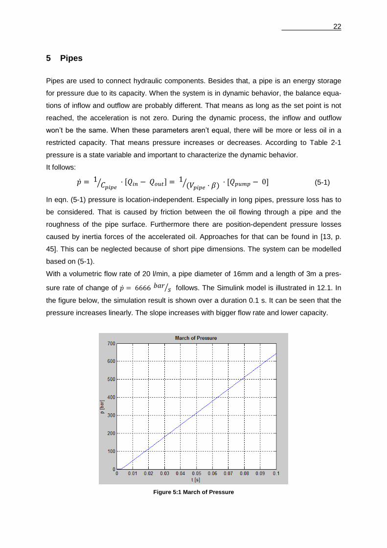
Pipes are used to connect hydraulic components. Besides that, a pipe is an energy storage
for pressure due to its capacity. When the system is in dynamic behavior, the balance equa-
tions of inflow and outflow are probably different. That means as long as the set point is not
reached, the acceleration is not zero. During the dynamic process, the inflow and outflow
won’t be the same. When these parameters aren’t equal, there will be more or less oil in a
restricted capacity. That means pressure increases or decreases. According to Table 2-1
pressure is a state variable and important to characterize the dynamic behavior.
It follows:
�̇� = 1 𝐶𝑝𝑖𝑝𝑒⁄ · [𝑄𝑖𝑛 − 𝑄𝑜𝑢𝑡] =
1(𝑉𝑝𝑖𝑝𝑒 · 𝛽)⁄ · [𝑄𝑝𝑢𝑚𝑝 − 0] (5-1)
In eqn. (5-1) pressure is location-independent. Especially in long pipes, pressure loss has to
be considered. That is caused by friction between the oil flowing through a pipe and the
roughness of the pipe surface. Furthermore there are position-dependent pressure losses
caused by inertia forces of the accelerated oil. Approaches for that can be found in [13, p.
45]. This can be neglected because of short pipe dimensions. The system can be modelled
based on (5-1).
With a volumetric flow rate of 20 l/min, a pipe diameter of 16mm and a length of 3m a pres-
sure rate of change of �̇� = 6666 𝑏𝑎𝑟 𝑠⁄ follows. The Simulink model is illustrated in 12.1. In
the figure below, the simulation result is shown over a duration 0.1 s. It can be seen that the
pressure increases linearly. The slope increases with bigger flow rate and lower capacity.
Figure 5:1 March of Pressure
23
6 Cylinder
In this section the theoretical considerations about the dynamic behavior of the cylinder shall
be explained. Based on these considerations the model can be created and finally the results
shall be discussed. In the circuit a differential cylinder with the dimension 200-100-500 is
used. Thereby the piston diameter is 200mm, the rod diameter is 100mm and the stroke is
500mm.
6.1 Theoretical Equations
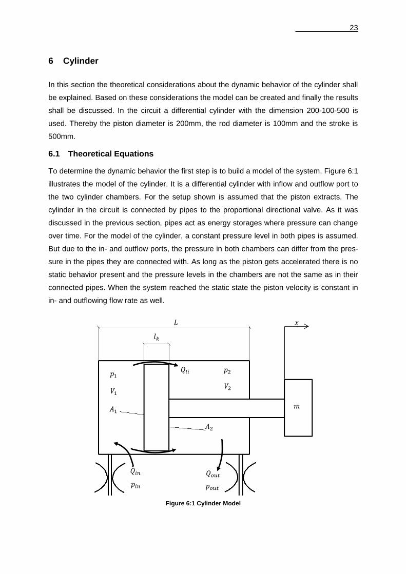
To determine the dynamic behavior the first step is to build a model of the system. Figure 6:1
illustrates the model of the cylinder. It is a differential cylinder with inflow and outflow port to
the two cylinder chambers. For the setup shown is assumed that the piston extracts. The
cylinder in the circuit is connected by pipes to the proportional directional valve. As it was
discussed in the previous section, pipes act as energy storages where pressure can change
over time. For the model of the cylinder, a constant pressure level in both pipes is assumed.
But due to the in- and outflow ports, the pressure in both chambers can differ from the pres-
sure in the pipes they are connected with. As long as the piston gets accelerated there is no
static behavior present and the pressure levels in the chambers are not the same as in their
connected pipes. When the system reached the static state the piston velocity is constant in
in- and outflowing flow rate as well.
Figure 6:1 Cylinder Model
𝑙𝑘
𝐿
𝑚
𝐴2
𝐴1
𝑉1
𝑝1 𝑝2
𝑉2
𝑄𝑙𝑖
𝑄𝑖𝑛
𝑝𝑖𝑛
𝑄𝑜𝑢𝑡
𝑝𝑜𝑢𝑡
𝑥
Cylinder 24
The cylinder’s energy storages are the chambers and the piston mass. The chambers store
fluidic energy where pressure can be obtained from. Whereas the piston mass stores kinetic
energy where acceleration, velocity and displacement can be obtained from. For the deriva-
tives of pressure 𝑝1 and 𝑝2 can be written:
�̇�1 =
1
𝐶1∫𝑄𝑠𝑡𝑜𝑟1
(6-1)
�̇�2 =1
𝐶2∫𝑄𝑠𝑡𝑜𝑟2 (6-2)
Thereby 𝑄𝑠𝑡𝑜𝑟1 respectively 𝑄𝑠𝑡𝑜𝑟2 are the sums of flow rates which stream in and out of each
chamber. The following equations can be written for the flow rate balances:
𝑄𝑠𝑡𝑜𝑟1 = 𝑄𝑖𝑛 − 𝑄𝑉1 − 𝑄𝑙𝑖 (6-3)
𝑄𝑠𝑡𝑜𝑟2 = 𝑄𝑉2 + 𝑄𝑙𝑖 −𝑄𝑜𝑢𝑡 (6-4)
In chamber 1 𝑄𝑠𝑡𝑜𝑟1 characterizes the sum of in- and outflow. The only incoming flow rate is
𝑄𝑖𝑛 which depends on the restriction and the pressure difference between chamber and pipe.
The inflow has to have the same amount of flow rate than the outflow. When the difference is
not balanced, the pressure increases or decreases due to a constant capacity. When there is
a certain flow rate 𝑄𝑖𝑛 streaming into the chamber, the same amount has to flow out. But
when the pressure level remains the same, capacity has to increase. With the assumption of
an almost constant bulk modulus, capacity can only increase when volume increases. For
this reason flow rate 𝑄𝑉1 has to be considered in that equation. It doesn’t drop out but in-
creases the volume. Likewise, the leakage flow rate 𝑄𝑙𝑖 has to be considered as well. It re-
sults from the pressure difference between the chambers and cannot be avoided because of
dimensional tolerances in the manufacturing process. A laminar flow profile is assumed in
the leakage gap. From these considerations follows:
𝑄𝑖𝑛 = 𝑠𝑖𝑔𝑛(𝑝𝑖𝑛 − 𝑝1) · 𝑘𝑑𝑟1 · 𝐴𝑑𝑟1√|𝑝𝑖𝑛 − 𝑝1| (6-5)
𝑄𝑉1 = �̇� · 𝐴1 (6-6)
𝑄𝑙𝑖 = 𝐺𝑔 · 𝛥𝑝12 = 𝜋 · 𝑑𝑚 · ℎ
3
12 · 𝜂 · 𝑙𝑘· 𝛥𝑝12 (6-7)
In the second chamber, there are the inflows 𝑄𝑉2 and the leakage 𝑄𝑙𝑖. 𝑄𝑉2 is caused by pis-
ton movement similar to 𝑄𝑉1. For a correct balance equation, the outflowing leakage from
chamber one has to be considered as an inflow for chamber two. It follows:
Cylinder 25
𝑄𝑜𝑢𝑡 = 𝑠𝑖𝑔𝑛(𝑝2 − 𝑝𝑜𝑢𝑡) · 𝑘𝑑𝑟2 · 𝐴𝑑𝑟2√|𝑝2 − 𝑝𝑜𝑢𝑡| (6-8)
𝑄𝑉2 = �̇� · 𝐴2 (6-9)
For the capacities can be written:
𝐶1 =
𝐾𝑏(𝑝)
𝑉1=
𝐾𝑏(𝑝)
𝑉1,0 + 𝑥 · 𝐴1
(6-10)
𝐶2 =𝐾𝑏(𝑝)
𝑉2=
𝐾𝑏(𝑝)
𝑉2,0 − 𝑥 · 𝐴2 (6-11)
The volumes 𝑉1,0 and 𝑉2,0 are the particular dead volumes. Both of them are assumed as 1%
of the total piston volume.
In the next step the balance equation of the forces shall be determined. Therefore all relevant
forces have to be considered.
𝑚�̈� = 𝐹1 − 𝐹2 − 𝐹𝑓𝑟 − 𝐹𝐿 (6-12)
With:
𝐹1 = 𝑝1 · 𝐴1 (6-13)
𝐹2 = 𝑝2 · 𝐴2 (6-14)
𝐹𝐿 is the load force and 𝐹𝑓𝑟 represents the friction force. Friction results when the piston dis-
places in the sleeve. This happens due to the contact between piston and the cylinder wall.
Thereby the influence of static, dynamic and viscous frictions has to be considered in the
same way. Viscous friction is caused by the leakage gap between cylinder wall and piston.
According to [13, p. 54] the influence of friction has to be considered especially in feedback
systems. For instance, when the static friction is very high, the system is not able to act on
small pressure differences. Firstly, static friction has to be overcome. For high piston veloci-
ties a huge extract of energy or a high damping can be a result. The exact advance projec-
tion is not possible. For this reason, the friction force is measured on the real system. Differ-
ent pressure differences at diverse speeds have to be collected for only one direction of
movement. With that set of data, the coefficients of a regression polynomial can be deter-
mined in a way that the polynomial fits the real measured behavior. Thereby, the objective is
to determine the dimension of these forces. During the simulation, certain values can be var-
ied to obtain better results. When high accuracy is needed, a polynomial for each direction of
movement has to be created. Another approach is illustrated in eqn. (6-15). According to [13,
p. 54] the friction force on a piston can be characterized as following:
Cylinder 26
𝐹𝑓𝑟 = 𝑠𝑖𝑔𝑛(�̇�) [𝐹𝑑𝑓 + 𝐹𝑠𝑓 · 𝑒−|�̇�|𝑇𝑉] + 𝑘 · �̇� (6-15)
With: 𝐹𝑑𝑓 - dynamic friction
𝐹𝑠𝑓 - static friction
𝑇𝑉 - decay constant
k - coefficient of viscous friction
The term of static friction decays exponentially with increasing velocity. The part of viscous
friction is constant and proportional to velocity. Due to the assumption of a laminar flow pro-
file in the leakage gap, factor k can be determined as following:
𝑘 = 𝐴 · 32 ·𝜂 · 𝑙𝑘
𝑑𝑚2 (6-16)
Due to the fact that it is not possible to measure the friction force of the real cylinder, eqn.
(6-15) shall be used. The static and dynamic friction forces shall be determined based on
normal force. The normal force of the piston is 330N. The friction coefficients are µ𝑠𝑓 = 0.12
and µ𝑑𝑓 = 0.05. From that follows:
𝐹𝑠𝑓 = µ𝑠𝑓 · 𝐹𝑁 (6-17)
𝐹𝑑𝑓 = µ𝑑𝑓 · 𝐹𝑁 (6-18)
6.2 Modelling with Simulink
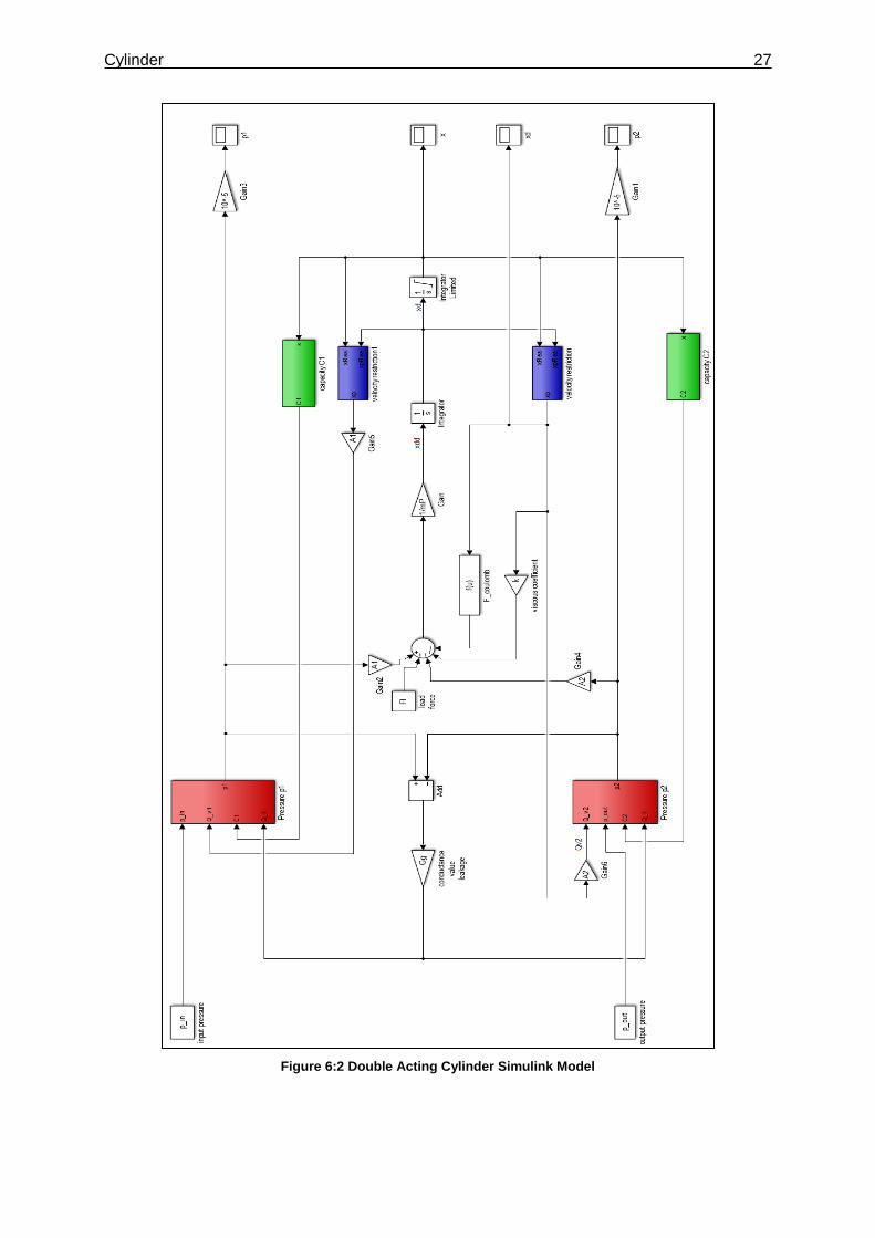
Based on the theoretical equations from the previous section, the model is created in Sim-
ulink. It is assumed that the proportional valve has already reached a fixed position. Conse-
quently the pressure levels in the input and output pipe are assumed to be constant. The
Simulink model of the actuator is shown in Figure 6:2 below. Equations (6-5) to (6-7) charac-
terize the input in the left chamber. Pressure builds up and the piston extends. Similar con-
siderations can be made for the right piston chamber. To model the march of pressure, eqn.
(6-1) respectively (6-2) is used. Pressure 𝑝1 and 𝑝2 are each modelled in a subsystem. The
capacity is modelled in a subsystem as well. It changes with a different spool position. The
maximum spool position was determined to 0.49m. The input for the capacity subsystems is
the limited velocity. The limited velocity also gets computed separately. Two switch-case
blocks are used to set the velocity to zero when the spool position is out of range of motion.
All subsystems are illustrated in 12.2.
Cylinder 27
Figure 6:2 Double Acting Cylinder Simulink Model
Cylinder 28
6.3 Results
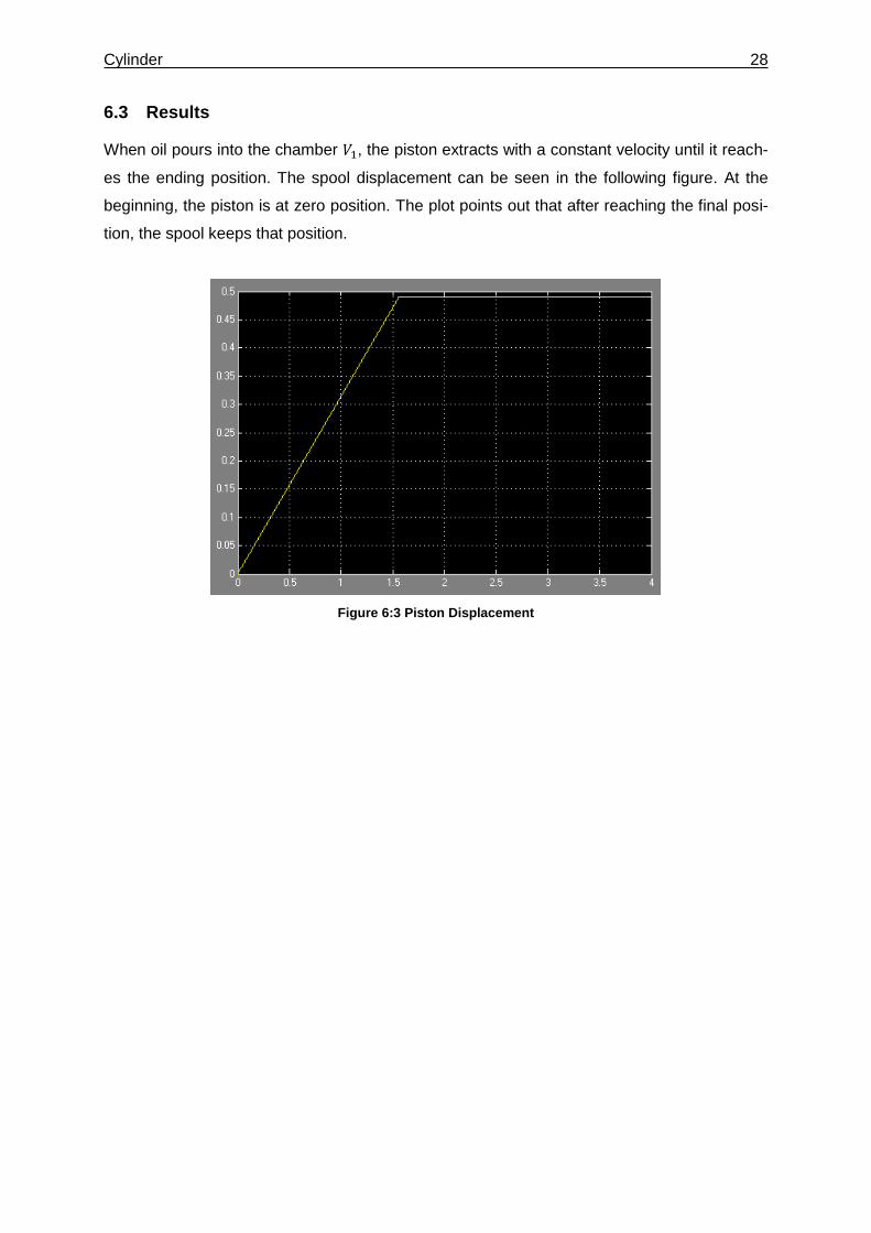
When oil pours into the chamber 𝑉1, the piston extracts with a constant velocity until it reach-
es the ending position. The spool displacement can be seen in the following figure. At the
beginning, the piston is at zero position. The plot points out that after reaching the final posi-
tion, the spool keeps that position.
Figure 6:3 Piston Displacement
29
7 Pressure Relief Valve
In this section the function, theoretical modelling and simulating of the pressure relief valve
(PRV) used in the circuit shall be explained. As already mentioned in section 2.2, pressure
relief vales are one main group of hydraulic valves. But they can be subdivided in pressure
relief, pressure reducing, differential pressure and pressure ratio valves [4, p. 152]. In the
circuit, the direct operated pressure relief valve “DBD NG10” is used which is produced by
Bosch Rexroth AG. It is direct operated because pressure has a straight connection to the
spool to act against the spring. The pressure relief valve acts in the hydraulic circuit as a se-
curity element and protects especially the pump from too high pressure levels. For this rea-
son there is a pressure relief valve mounted parallel to the pump in every hydraulic circuit.
7.1 Theoretical Considerations
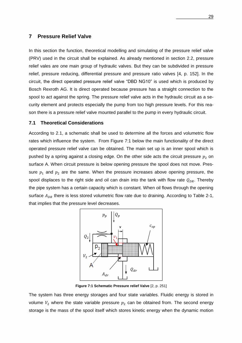
According to 2.1, a schematic shall be used to determine all the forces and volumetric flow
rates which influence the system. From Figure 7:1 below the main functionality of the direct
operated pressure relief valve can be obtained. The main set up is an inner spool which is
pushed by a spring against a closing edge. On the other side acts the circuit pressure 𝑝2 on
surface A. When circuit pressure is below opening pressure the spool does not move. Pres-
sure 𝑝1 and 𝑝2 are the same. When the pressure increases above opening pressure, the
spool displaces to the right side and oil can drain into the tank with flow rate 𝑄𝐷𝑅. Thereby
the pipe system has a certain capacity which is constant. When oil flows through the opening
surface 𝐴𝐷𝑅 there is less stored volumetric flow rate due to draining. According to Table 2-1,
that implies that the pressure level decreases.
Figure 7:1 Schematic Pressure relief Valve [2, p. 251]
The system has three energy storages and four state variables. Fluidic energy is stored in
volume 𝑉2 where the state variable pressure 𝑝2 can be obtained from. The second energy
storage is the mass of the spool itself which stores kinetic energy when the dynamic motion
x
𝑄𝑝
𝑄𝑑𝑟 𝐴𝑑𝑟
𝑉2
𝑄2
𝑐𝑠𝑝
𝑣1
𝑝𝑝
Pressure Relief Valve 30
starts. This storage is connected to the state variable spool acceleration �̈�. From acceleration
the other state variables spool velocity �̇� and displacement 𝑥 can be determined. Also con-
nected to state variable displacement is the spring which stores potential energy. Now, the
equations for all energy storages shall be determined to obtain the state variables needed.
Firstly, the state variable 𝑝2 shall be determined. According to Table 2-1 the following ex-
pression can be found:
�̇�2 =1
𝐶2∫𝑄𝑠𝑡𝑜𝑟 (7-1)
The capacity 𝐶2 can be determined to
𝐶2 = 𝑉2 · 𝛽𝑏 (7-2)
where 𝛽𝑏 is the reciprocal bulk modulus of the hydraulic oil and 𝑉2 the volume which can
change when spool displaces.
𝑉2 = 𝑉2 + 𝑥 · 𝐴 (7-3)
The stored volumetric flow rate in volume 𝑉2 is the difference between outflow and inflow.
When there is more incoming flow rate than flow rate going out, the pressure starts to in-
crease. For the considerations of the pressure relief valve the volume 𝑉2 has to be treated as
a volume. But this can only be related to the PRV itself. This volume is not incorporated in
the considerations of the whole circuit because it is just too small. For the considerations of
the whole circuit the PRV is just seen as an open-loop control element to release pressure
level when needed.
The stored volumetric flow rate can be written as following:
𝑄𝑠𝑡𝑜𝑟 = 𝑄2 − 𝑄𝑉2 (7-4)
with
𝑄𝑉2 = �̇� · 𝐴 (7-5)
𝑄2 = 𝜋 · 𝑑𝑚 · ℎ
3
12 · 𝜂 · 𝑙𝛥𝑝 = 𝐺 · 𝛥𝑝 = 𝐺 · (𝑝𝑝 − 𝑝2)
(7-6,
[4, p. 62])
To flow into volume 𝑉2 the oil has to pass a resistance which is assumed as a thin leakage
gap. Following that assumption it can be concluded that the flow rate in that gap is laminar
which makes it independent from velocity. It only depends on the geometrics and the pres-
sure difference between incoming pressure 𝑝𝑝 and 𝑝2. The geometrics can be summed up to
resistance factor 𝐺.
The overall balance for the flow rates through the valve can be obtained when dynamic mo-
tion is assumed. The drain flow rate 𝑄𝑑𝑟 and 𝑄2 in summation has to be the same as what
comes into the valve.
Pressure Relief Valve 31
𝑄𝑝 = 𝑄2 + 𝑄𝑑𝑟 (7-7)
In the next step the static, dynamic and balance equations to obtain the state variable dis-
placement, velocity and acceleration shall be found. According to Figure 7:1 the static bal-
ance equation can be obtained to:
𝑝2𝐴 = 𝐹𝑝2 = 𝐹𝑠𝑝(𝑥) (7-8)
with the spring force 𝐹𝑠𝑝(𝑥) of:
𝐹𝑠𝑝(𝑥) = 𝑐𝑠𝑝 (𝑥 − 𝑥𝑖𝑛𝑖𝑡) (7-9)
When the pressure force in chamber 𝑉2 overcomes 𝐹𝑠𝑝(𝑥) the valve spool opens. The volu-
metric flow rate 𝑄𝐷𝑅 can be determined to:
𝑄𝑑𝑟 = √1
𝜁 · √
2
𝜌 · 𝐴 · √|𝛥𝑝| = 𝑘𝑑𝑟 𝐴𝑑𝑟 √𝑝𝑝 (7-10)
In (7-10) is assumed that the tank pressure is equal to reference pressure. When the spool
displaces and enables 𝑄𝑑𝑟 to flow through, dynamic behavior takes place. Caused by the
dynamic displacement of the spool, friction force 𝐹𝑓𝑟 and flow force 𝐹𝑓𝑟 act against the open-
ing motion. The flow force has a significant impact on the dynamic behavior of hydraulic
valves in general. Most valves are designed as linear spool valves with several controlling
edges. When the spool starts to open, the inflowing oil exerts radial and axial forces to the
spool. The higher the differential pressure between the two valve ports, the higher the oil’s
velocity is. When the velocity increases the flow force increases as well because flow force
can be determined by using the principle of linear momentum. By assuming oil enters the
valve through an annular gap, the controlling edge deflects the oil in a way that it impacts the
spool under a certain angle 𝜀. That causes a flow force which is aligned with the closing di-
rection. As already mentioned, that flow force has radial and axial components. The radial
components act with the same absolute value on the circumference and become zero.
Whereas the axial components can be obtained for steady flow to:
𝐹𝑓𝑓 = 𝜌 · 𝑄𝑑𝑟 · 𝑣1 · cos(𝜀1) = 𝜌 ·𝑄²𝑑𝑟𝐴𝑑𝑟
· cos(𝜀1) (7-11)
For unsteady flow the dynamic flow force term
𝐹𝑓𝑓,𝑑𝑦𝑛 = 𝜌 · l ·𝑑𝑄𝑑𝑟dt
(7-12)
can be added but according to [4, p. 78] it is relatively small compared to the static term.
Hence only the static flow term in (7-11) shall be used. Another important effect to determine
is the friction force. The spool is installed in sleeve and is directly in contact with it. Due to
manufacturing tolerances there are small gaps between spool and sleeve which are filled
Pressure Relief Valve 32
with leakage oil. Thus, boundary lubrication is present in the system. Friction always de-
pends on the direction motion. It always acts in opposite direction. To determine the friction
force the same approach as in 6.1 shall be used.
𝐹𝑓𝑟 = 𝑠𝑖𝑔𝑛(�̇�) [𝐹𝑑𝑓 + 𝐹𝑠𝑓 · 𝑒−|�̇�|𝑇𝑉] + 𝑘 · �̇�
(7-13,
[13, p. 54])
After determining all the relevant forces the dynamic behavior can be expressed to
𝑚�̈� = 𝐹𝑝2 − 𝐹𝑠𝑝(𝑥) − 𝐹𝑓𝑟(�̇�) − 𝐹𝑓𝑓(𝑥, 𝑝2) (7-14)
Eqn. (7-14) points out that only the pressure force 𝐹𝑝2 acts on the spool in opening direction.
The spring force 𝐹𝑠𝑝, friction force 𝐹𝑓𝑟 and flow force 𝐹𝑓𝑓 act towards closing direction. From
that perspective, the pressure relief valve characteristic can be obtained. 𝐹𝑠𝑝 represents a
static offset for the valve to open while 𝐹𝑓𝑟 is an almost constant value and not absolutely
necessary for the qualitative characteristic. But the flow force is even more relevant. It shows
a quadratic relationship to 𝐹𝑓𝑓. If the flow rate through the valve increases, the flow force in-
creases quadratically. It can be concluded that the pressure level has to increase as well to
maintain that drain flow rate to the tank. That behavior can be observed when looking at the
characteristic curves given by the manufacturer.
Figure 7:2 shows the qualitative characteristics of a direct-operated (a) and a pilot-operated
(b) pressure relief valve. As a comparison, curve c shows an ideal behavior. Figure 7:3
shows the real valve curves for different levels pressure levels. It is illustrated that the flow
force influence is almost not present for high pressure levels. At low pressure levels (curve 1)
almost without non static pressure offset it is remarkably good noticeable that the flow force
plays the main role. Below curve 1, no operation is possible.
Finally, a block diagram can be drawn to determine the connection of all presented equa-
tions. Figure 7:4 illustrates the qualitative block diagram which is built on the found relation-
Figure 7:2 Qualitative Pressure Relief Curves Figure 7:3 PRV Curves from Datasheet
a
b
c
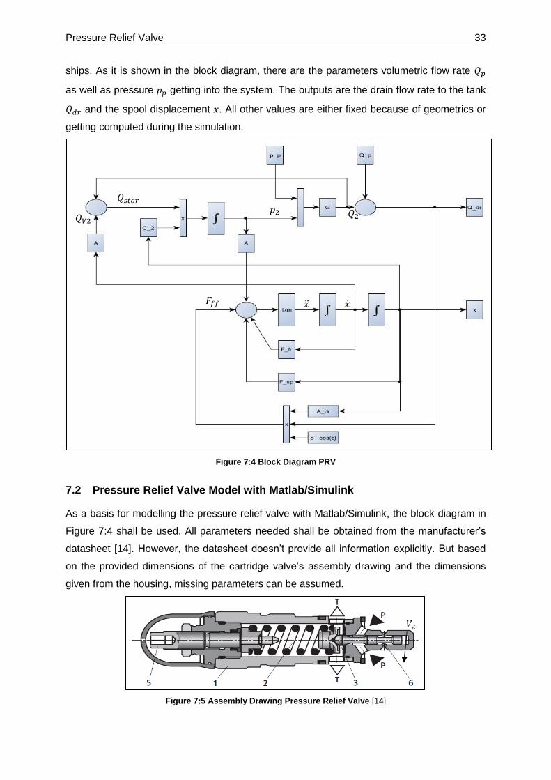
Pressure Relief Valve 33
ships. As it is shown in the block diagram, there are the parameters volumetric flow rate 𝑄𝑝
as well as pressure 𝑝𝑝 getting into the system. The outputs are the drain flow rate to the tank
𝑄𝑑𝑟 and the spool displacement 𝑥. All other values are either fixed because of geometrics or
getting computed during the simulation.
Figure 7:4 Block Diagram PRV
7.2 Pressure Relief Valve Model with Matlab/Simulink
As a basis for modelling the pressure relief valve with Matlab/Simulink, the block diagram in
Figure 7:4 shall be used. All parameters needed shall be obtained from the manufacturer’s
datasheet [14]. However, the datasheet doesn’t provide all information explicitly. But based
on the provided dimensions of the cartridge valve’s assembly drawing and the dimensions
given from the housing, missing parameters can be assumed.
Figure 7:5 Assembly Drawing Pressure Relief Valve [14]
𝑄𝑠𝑡𝑜𝑟 𝑝2 𝑄2
𝐹𝑓𝑓 �̈� �̇�
𝑄𝑉2
𝑉2
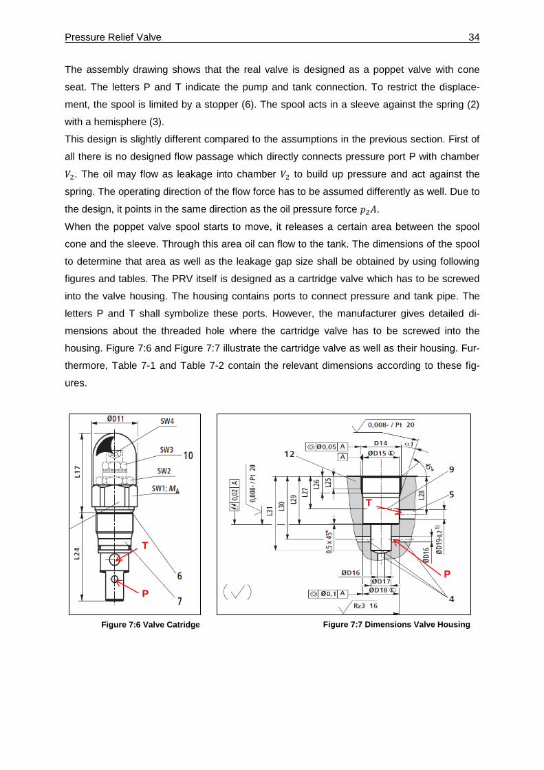
Pressure Relief Valve 34
P
T
P
T
The assembly drawing shows that the real valve is designed as a poppet valve with cone
seat. The letters P and T indicate the pump and tank connection. To restrict the displace-
ment, the spool is limited by a stopper (6). The spool acts in a sleeve against the spring (2)
with a hemisphere (3).
This design is slightly different compared to the assumptions in the previous section. First of
all there is no designed flow passage which directly connects pressure port P with chamber
𝑉2. The oil may flow as leakage into chamber 𝑉2 to build up pressure and act against the
spring. The operating direction of the flow force has to be assumed differently as well. Due to
the design, it points in the same direction as the oil pressure force 𝑝2𝐴.
When the poppet valve spool starts to move, it releases a certain area between the spool
cone and the sleeve. Through this area oil can flow to the tank. The dimensions of the spool
to determine that area as well as the leakage gap size shall be obtained by using following
figures and tables. The PRV itself is designed as a cartridge valve which has to be screwed
into the valve housing. The housing contains ports to connect pressure and tank pipe. The
letters P and T shall symbolize these ports. However, the manufacturer gives detailed di-
mensions about the threaded hole where the cartridge valve has to be screwed into the
housing. Figure 7:6 and Figure 7:7 illustrate the cartridge valve as well as their housing. Fur-
thermore, Table 7-1 and Table 7-2 contain the relevant dimensions according to these fig-
ures.
Figure 7:6 Valve Catridge Figure 7:7 Dimensions Valve Housing
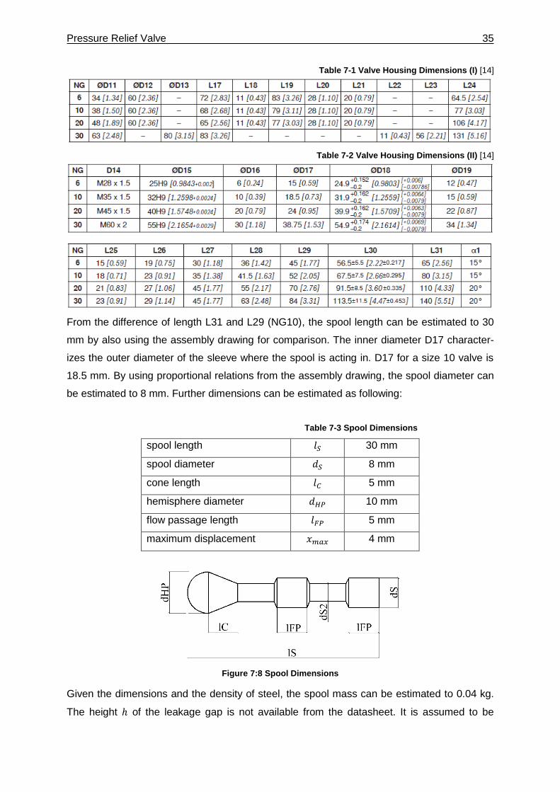
Pressure Relief Valve 35
Table 7-1 Valve Housing Dimensions (I) [14]
Table 7-2 Valve Housing Dimensions (II) [14]
From the difference of length L31 and L29 (NG10), the spool length can be estimated to 30
mm by also using the assembly drawing for comparison. The inner diameter D17 character-
izes the outer diameter of the sleeve where the spool is acting in. D17 for a size 10 valve is
18.5 mm. By using proportional relations from the assembly drawing, the spool diameter can
be estimated to 8 mm. Further dimensions can be estimated as following:
Table 7-3 Spool Dimensions
spool length 𝑙𝑆 30 mm
spool diameter 𝑑𝑆 8 mm
cone length 𝑙𝐶 5 mm
hemisphere diameter 𝑑𝐻𝑃 10 mm
flow passage length 𝑙𝐹𝑃 5 mm
maximum displacement 𝑥𝑚𝑎𝑥 4 mm
Figure 7:8 Spool Dimensions
Given the dimensions and the density of steel, the spool mass can be estimated to 0.04 kg.
The height ℎ of the leakage gap is not available from the datasheet. It is assumed to be
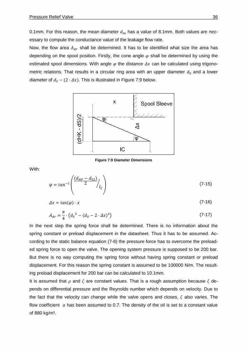
Pressure Relief Valve 36
0.1mm. For this reason, the mean diameter 𝑑𝑚 has a value of 8.1mm. Both values are nec-
essary to compute the conductance value of the leakage flow rate.
Now, the flow area 𝐴𝑑𝑟 shall be determined. It has to be identified what size the area has
depending on the spool position. Firstly, the cone angle 𝜑 shall be determined by using the
estimated spool dimensions. With angle 𝜑 the distance 𝛥𝑥 can be calculated using trigono-
metric relations. That results in a circular ring area with an upper diameter 𝑑𝑆 and a lower
diameter of 𝑑𝑆 − (2 · 𝛥𝑥). This is illustrated in Figure 7:9 below.
Figure 7:9 Diameter Dimensions
With:
𝜑 = 𝑡𝑎𝑛−1(
(𝑑𝐻𝑃 − 𝑑𝑆2)2
𝑙𝐶⁄ ) (7-15)
𝛥𝑥 = tan (𝜑) · 𝑥 (7-16)
𝐴𝑑𝑟 =𝜋
4· (𝑑𝑆
2 − (𝑑𝑆 − 2 · 𝛥𝑥)²) (7-17)
In the next step the spring force shall be determined. There is no information about the
spring constant or preload displacement in the datasheet. Thus it has to be assumed. Ac-
cording to the static balance equation (7-8) the pressure force has to overcome the preload-
ed spring force to open the valve. The opening system pressure is supposed to be 200 bar.
But there is no way computing the spring force without having spring constant or preload
displacement. For this reason the spring constant is assumed to be 100000 N/m. The result-
ing preload displacement for 200 bar can be calculated to 10.1mm.
It is assumed that 𝜌 and 𝜁 are constant values. That is a rough assumption because 𝜁 de-
pends on differential pressure and the Reynolds number which depends on velocity. Due to
the fact that the velocity can change while the valve opens and closes, 𝜁 also varies. The
flow coefficient 𝛼 has been assumed to 0.7. The density of the oil is set to a constant value
of 880 kg/m³.
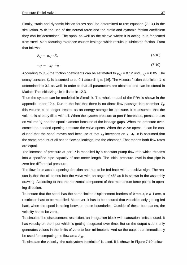
Pressure Relief Valve 37
Finally, static and dynamic friction forces shall be determined to use equation (7-13,) in the
simulation. With the use of the normal force and the static and dynamic friction coefficient
they can be determined. The spool as well as the sleeve where it is acting in is fabricated
from steel. Manufacturing tolerance causes leakage which results in lubricated friction. From
that follows:
𝐹𝑠𝑓 = µ𝑠𝑓 · 𝐹𝑁 (7-18)
𝐹𝑑𝑓 = µ𝑑𝑓 · 𝐹𝑁 (7-19)
According to [15] the friction coefficients can be estimated to µ𝑠𝑓 = 0.12 und µ𝑑𝑓 = 0.05. The
decay constant 𝑇𝑉 is assumed to be 0.1 according to [16]. The viscous friction coefficient 𝑘 is
determined to 0.1 as well. In order to that all parameters are obtained and can be stored in
Matlab. The initializing file is listed in 12.3.
Then the system can be modelled in Simulink. The whole model of the PRV is shown in the
appendix under 12.4. Due to the fact that there is no direct flow passage into chamber 𝑉2,
this volume is no longer treated as an energy storage for pressure. It is assumed that the
volume is already filled with oil. When the system pressure at port P increases, pressure acts
on volume 𝑉2 and the spool diameter because of the leakage gaps. When the pressure over-
comes the needed opening pressure the valve opens. When the valve opens, it can be con-
cluded that the spool moves and because of that 𝑉2 increases on �̇� · 𝐴𝑆. It is assumed that
the same amount of oil has to flow as leakage into the chamber. That means both flow rates
are equal.
The increase of pressure at port P is modelled by a constant pump flow rate which streams
into a specified pipe capacity of one meter length. The initial pressure level in that pipe is
zero bar differential pressure.
The flow force acts in opening direction and has to be fed back with a positive sign. The rea-
son is that the oil comes into the valve with an angle of 45° as it is shown in the assembly
drawing. According to that the horizontal component of that momentum force points in open-
ing direction.
To ensure that the spool has the same limited displacement barriers of 0 𝑚𝑚 ⩽ 𝑥 ⩽ 4 𝑚𝑚, a
restriction hast to be modelled. Moreover, it has to be ensured that velocities only getting fed
back when the spool is acting between these boundaries. Outside of these boundaries, the
velocity has to be zero.
To simulate the displacement restriction, an integration block with saturation limits is used. It
has velocity on the input which is getting integrated over time. But on the output side it only
generates values in the limits of zero to four millimeters. And so the output can immediately
be used for computing the flow area 𝐴𝑑𝑟.
To simulate the velocity, the subsystem ‘restriction’ is used. It is shown in Figure 7:10 below.
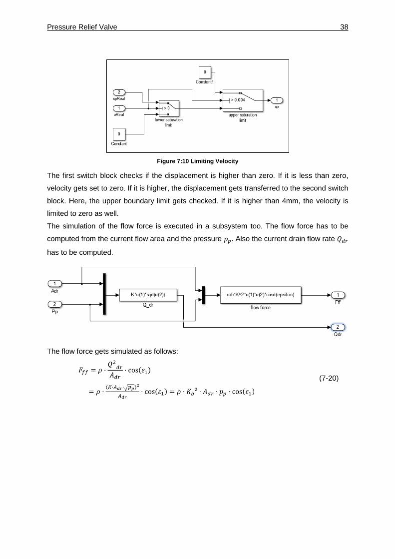
Pressure Relief Valve 38
Figure 7:10 Limiting Velocity
The first switch block checks if the displacement is higher than zero. If it is less than zero,
velocity gets set to zero. If it is higher, the displacement gets transferred to the second switch
block. Here, the upper boundary limit gets checked. If it is higher than 4mm, the velocity is
limited to zero as well.
The simulation of the flow force is executed in a subsystem too. The flow force has to be
computed from the current flow area and the pressure 𝑝𝑝. Also the current drain flow rate 𝑄𝑑𝑟
has to be computed.
The flow force gets simulated as follows:
𝐹𝑓𝑓 = 𝜌 ·𝑄2𝑑𝑟𝐴𝑑𝑟
· cos(𝜀1)
= 𝜌 ·(𝐾·𝐴𝑑𝑟·√𝑝𝑝)
2
𝐴𝑑𝑟· cos(𝜀1) = 𝜌 · 𝐾𝑏² · 𝐴𝑑𝑟 · 𝑝𝑝 · cos(𝜀1)
(7-20)
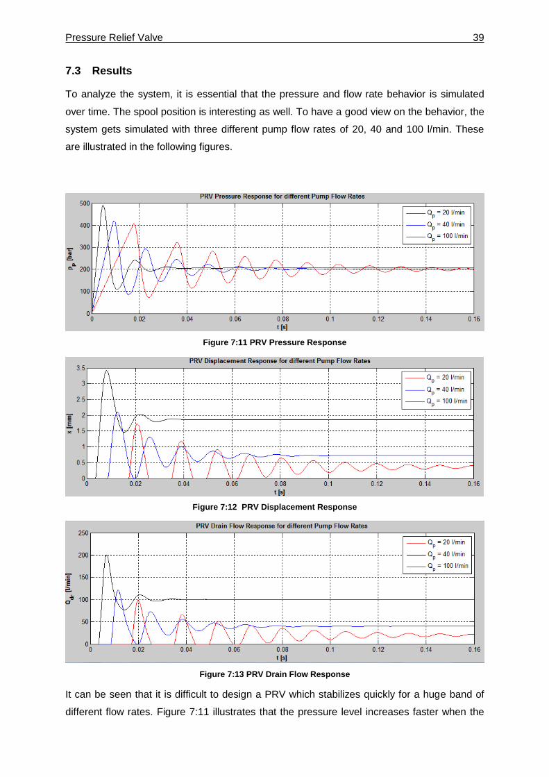
Pressure Relief Valve 39
7.3 Results
To analyze the system, it is essential that the pressure and flow rate behavior is simulated
over time. The spool position is interesting as well. To have a good view on the behavior, the
system gets simulated with three different pump flow rates of 20, 40 and 100 l/min. These
are illustrated in the following figures.
Figure 7:11 PRV Pressure Response
Figure 7:12 PRV Displacement Response
Figure 7:13 PRV Drain Flow Response
It can be seen that it is difficult to design a PRV which stabilizes quickly for a huge band of
different flow rates. Figure 7:11 illustrates that the pressure level increases faster when the
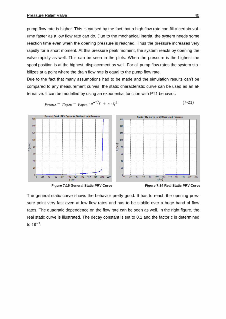
Pressure Relief Valve 40
pump flow rate is higher. This is caused by the fact that a high flow rate can fill a certain vol-
ume faster as a low flow rate can do. Due to the mechanical inertia, the system needs some
reaction time even when the opening pressure is reached. Thus the pressure increases very
rapidly for a short moment. At this pressure peak moment, the system reacts by opening the
valve rapidly as well. This can be seen in the plots. When the pressure is the highest the
spool position is at the highest, displacement as well. For all pump flow rates the system sta-
bilizes at a point where the drain flow rate is equal to the pump flow rate.
Due to the fact that many assumptions had to be made and the simulation results can’t be
compared to any measurement curves, the static characteristic curve can be used as an al-
ternative. It can be modelled by using an exponential function with PT1 behavior.
𝑝𝑠𝑡𝑎𝑡𝑖𝑐 = 𝑝𝑜𝑝𝑒𝑛 − 𝑝𝑜𝑝𝑒𝑛 · 𝑒−𝑄 𝑇⁄ + 𝑐 · 𝑄2 (7-21)
The general static curve shows the behavior pretty good. It has to reach the opening pres-
sure point very fast even at low flow rates and has to be stabile over a huge band of flow
rates. The quadratic dependence on the flow rate can be seen as well. In the right figure, the
real static curve is illustrated. The decay constant is set to 0.1 and the factor c is determined
to 10−7.
Figure 7:14 Real Static PRV Curve Figure 7:15 General Static PRV Curve
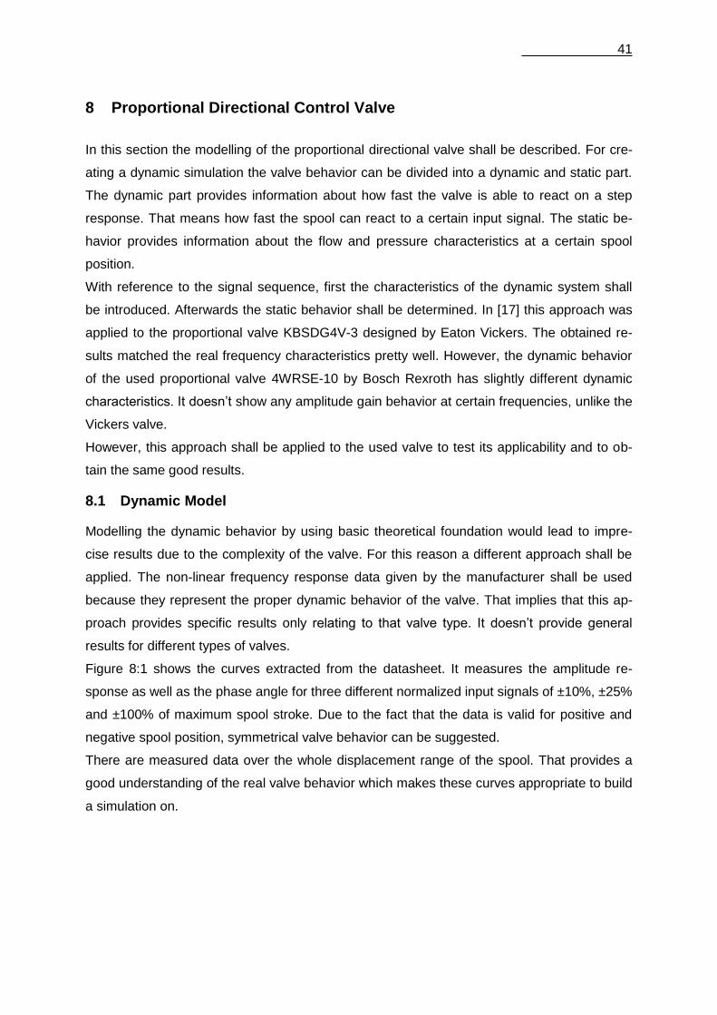
41
8 Proportional Directional Control Valve
In this section the modelling of the proportional directional valve shall be described. For cre-
ating a dynamic simulation the valve behavior can be divided into a dynamic and static part.
The dynamic part provides information about how fast the valve is able to react on a step
response. That means how fast the spool can react to a certain input signal. The static be-
havior provides information about the flow and pressure characteristics at a certain spool
position.
With reference to the signal sequence, first the characteristics of the dynamic system shall
be introduced. Afterwards the static behavior shall be determined. In [17] this approach was
applied to the proportional valve KBSDG4V-3 designed by Eaton Vickers. The obtained re-
sults matched the real frequency characteristics pretty well. However, the dynamic behavior
of the used proportional valve 4WRSE-10 by Bosch Rexroth has slightly different dynamic
characteristics. It doesn’t show any amplitude gain behavior at certain frequencies, unlike the
Vickers valve.
However, this approach shall be applied to the used valve to test its applicability and to ob-
tain the same good results.
8.1 Dynamic Model
Modelling the dynamic behavior by using basic theoretical foundation would lead to impre-
cise results due to the complexity of the valve. For this reason a different approach shall be
applied. The non-linear frequency response data given by the manufacturer shall be used
because they represent the proper dynamic behavior of the valve. That implies that this ap-
proach provides specific results only relating to that valve type. It doesn’t provide general
results for different types of valves.
Figure 8:1 shows the curves extracted from the datasheet. It measures the amplitude re-
sponse as well as the phase angle for three different normalized input signals of ±10%, ±25%
and ±100% of maximum spool stroke. Due to the fact that the data is valid for positive and
negative spool position, symmetrical valve behavior can be suggested.
There are measured data over the whole displacement range of the spool. That provides a
good understanding of the real valve behavior which makes these curves appropriate to build
a simulation on.
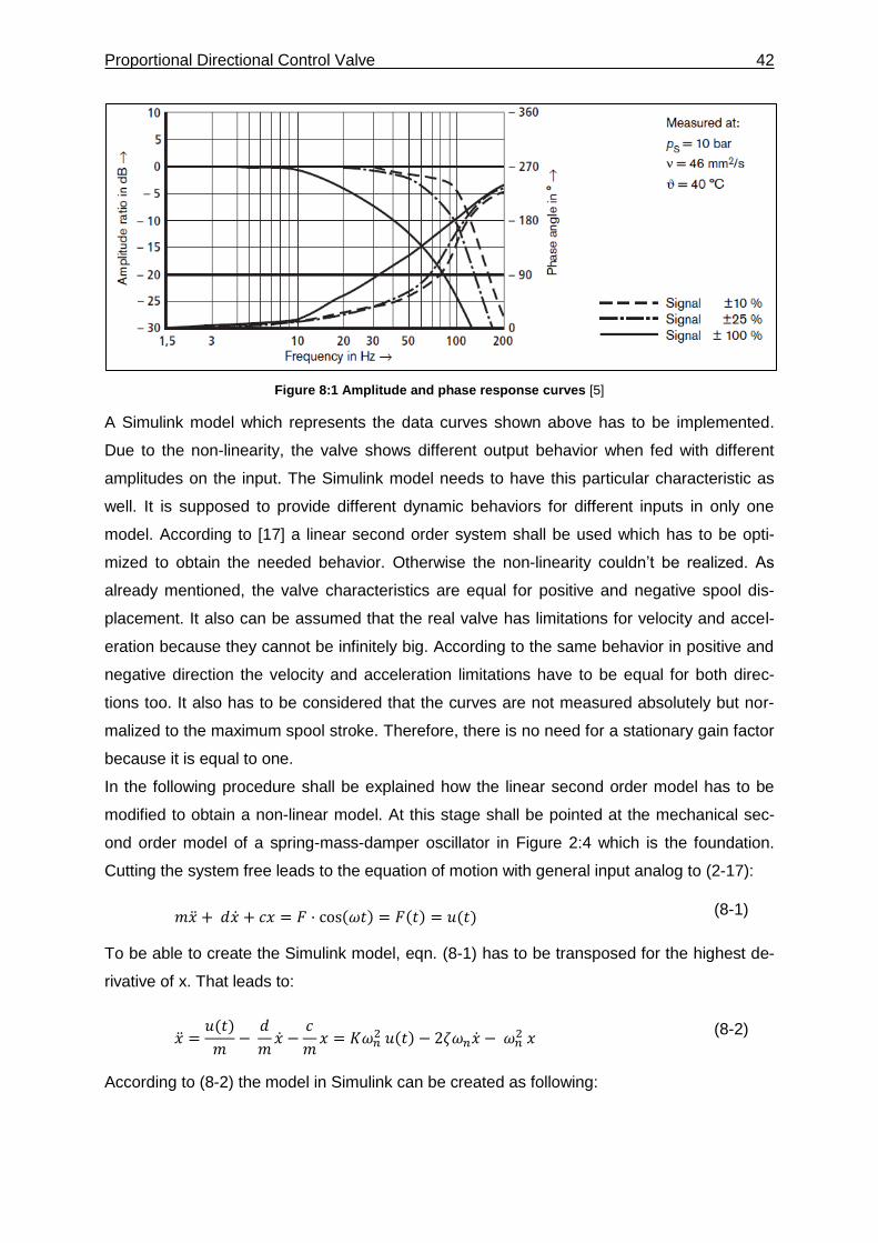
Proportional Directional Control Valve 42
Figure 8:1 Amplitude and phase response curves [5]
A Simulink model which represents the data curves shown above has to be implemented.
Due to the non-linearity, the valve shows different output behavior when fed with different
amplitudes on the input. The Simulink model needs to have this particular characteristic as
well. It is supposed to provide different dynamic behaviors for different inputs in only one
model. According to [17] a linear second order system shall be used which has to be opti-
mized to obtain the needed behavior. Otherwise the non-linearity couldn’t be realized. As
already mentioned, the valve characteristics are equal for positive and negative spool dis-
placement. It also can be assumed that the real valve has limitations for velocity and accel-
eration because they cannot be infinitely big. According to the same behavior in positive and
negative direction the velocity and acceleration limitations have to be equal for both direc-
tions too. It also has to be considered that the curves are not measured absolutely but nor-
malized to the maximum spool stroke. Therefore, there is no need for a stationary gain factor
because it is equal to one.
In the following procedure shall be explained how the linear second order model has to be
modified to obtain a non-linear model. At this stage shall be pointed at the mechanical sec-
ond order model of a spring-mass-damper oscillator in Figure 2:4 which is the foundation.
Cutting the system free leads to the equation of motion with general input analog to (2-17):
𝑚�̈� + 𝑑�̇� + 𝑐𝑥 = 𝐹 · cos(𝜔𝑡) = 𝐹(𝑡) = 𝑢(𝑡) (8-1)
To be able to create the Simulink model, eqn. (8-1) has to be transposed for the highest de-
rivative of x. That leads to:
�̈� =𝑢(𝑡)
𝑚− 𝑑
𝑚�̇� −
𝑐
𝑚𝑥 = 𝐾𝜔𝑛
2 𝑢(𝑡) − 2𝜁𝜔𝑛�̇� − 𝜔𝑛2 𝑥
(8-2)
According to (8-2) the model in Simulink can be created as following:
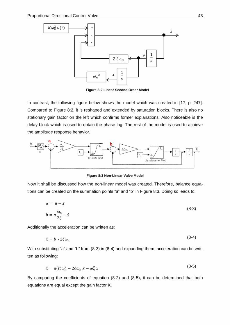
Proportional Directional Control Valve 43
In contrast, the following figure below shows the model which was created in [17, p. 247].
Compared to Figure 8:2, it is reshaped and extended by saturation blocks. There is also no
stationary gain factor on the left which confirms former explanations. Also noticeable is the
delay block which is used to obtain the phase lag. The rest of the model is used to achieve
the amplitude response behavior.
Figure 8:3 Non-Linear Valve Model
Now it shall be discussed how the non-linear model was created. Therefore, balance equa-
tions can be created on the summation points “a” and “b” in Figure 8:3. Doing so leads to:
𝑎 = �̅� − �̅�
𝑏 = 𝑎𝜔𝑛2𝜁− �̇�
(8-3)
Additionally the acceleration can be written as:
�̈� = 𝑏 · 2𝜁𝜔𝑛 (8-4)
With substituting “a” and “b” from (8-3) in (8-4) and expanding them, acceleration can be writ-
ten as following:
�̈� = 𝑢(𝑡)𝜔𝑛2 − 2𝜁𝜔𝑛 �̇� − 𝜔𝑛
2 𝑥 (8-5)
By comparing the coefficients of equation (8-2) and (8-5), it can be determined that both
equations are equal except the gain factor K.
Figure 8:2 Linear Second Order Model
a b
�̈�
�̇�
𝐾𝜔𝑛2 𝑢(𝑡) +
-
-
1
𝑠
1
𝑠 2 ζ 𝜔𝑛
𝜔𝑛² 𝑥
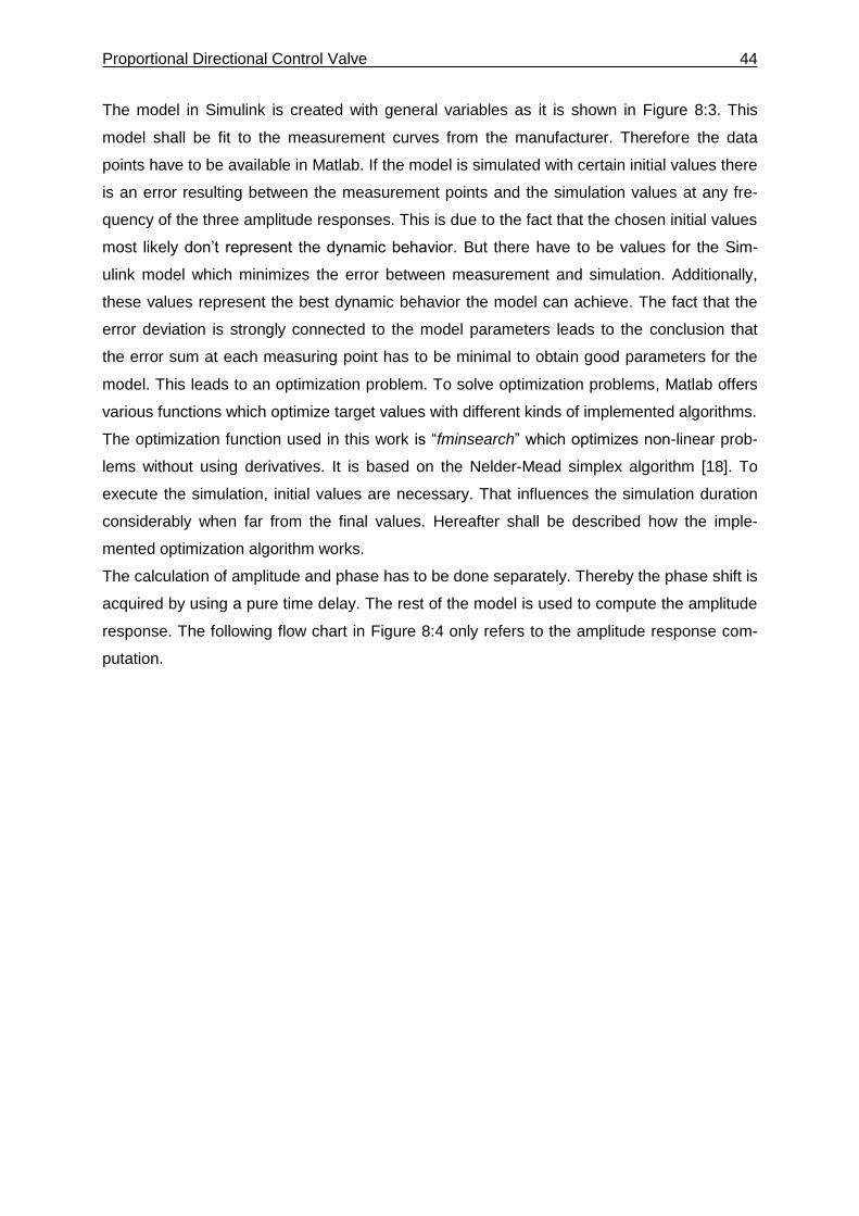
Proportional Directional Control Valve 44
The model in Simulink is created with general variables as it is shown in Figure 8:3. This
model shall be fit to the measurement curves from the manufacturer. Therefore the data
points have to be available in Matlab. If the model is simulated with certain initial values there
is an error resulting between the measurement points and the simulation values at any fre-
quency of the three amplitude responses. This is due to the fact that the chosen initial values
most likely don’t represent the dynamic behavior. But there have to be values for the Sim-
ulink model which minimizes the error between measurement and simulation. Additionally,
these values represent the best dynamic behavior the model can achieve. The fact that the
error deviation is strongly connected to the model parameters leads to the conclusion that
the error sum at each measuring point has to be minimal to obtain good parameters for the
model. This leads to an optimization problem. To solve optimization problems, Matlab offers
various functions which optimize target values with different kinds of implemented algorithms.
The optimization function used in this work is “fminsearch” which optimizes non-linear prob-
lems without using derivatives. It is based on the Nelder-Mead simplex algorithm [18]. To
execute the simulation, initial values are necessary. That influences the simulation duration
considerably when far from the final values. Hereafter shall be described how the imple-
mented optimization algorithm works.
The calculation of amplitude and phase has to be done separately. Thereby the phase shift is
acquired by using a pure time delay. The rest of the model is used to compute the amplitude
response. The following flow chart in Figure 8:4 only refers to the amplitude response com-
putation.
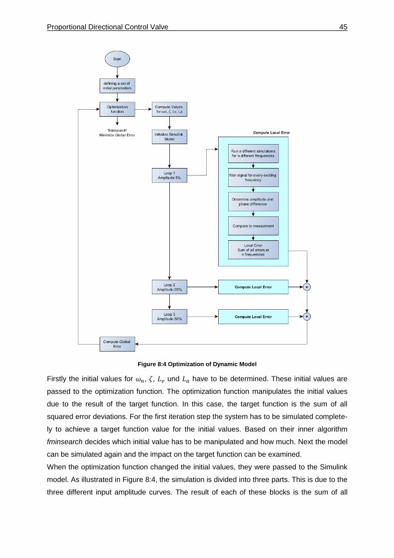
Proportional Directional Control Valve 45
Figure 8:4 Optimization of Dynamic Model
Firstly the initial values for 𝜔𝑛, 𝜁, 𝐿𝑣 und 𝐿𝑎 have to be determined. These initial values are
passed to the optimization function. The optimization function manipulates the initial values
due to the result of the target function. In this case, the target function is the sum of all
squared error deviations. For the first iteration step the system has to be simulated complete-
ly to achieve a target function value for the initial values. Based on their inner algorithm
fminsearch decides which initial value has to be manipulated and how much. Next the model
can be simulated again and the impact on the target function can be examined.
When the optimization function changed the initial values, they were passed to the Simulink
model. As illustrated in Figure 8:4, the simulation is divided into three parts. This is due to the
three different input amplitude curves. The result of each of these blocks is the sum of all
Proportional Directional Control Valve 46
local squared errors from measurement to simulation point at a certain frequency. According
to [17] the global error is computed as following:
𝐹𝑔𝑙𝑜𝑏𝑎𝑙 = 4 · 𝐹𝑙𝑜𝑐𝑎𝑙,10% + 𝐹𝑙𝑜𝑐𝑎𝑙,25% + 𝐹𝑙𝑜𝑐𝑎𝑙,100% (8-6)
The local error deviation 𝐹𝑙𝑜𝑐𝑎𝑙,10% is weighted with a factor of 4. This is why the valve oper-
ates most of the time around the middle position to adjust the flow rate very precisely when
controlling an actuator position. Hence it is necessary to put more effort in a good approxima-
tion of that curve.
To compute the local error, a few steps are important. Firstly, amplitude response measure-
ment data at different frequencies is needed. These have to be extracted from the datasheet.
The used measurement data is illustrated in 12.5. When the Simulink model is supplied with
a sinusoidal signal, nonlinearities occur due to the saturation blocks. The saturation blocks
are essential to fit the model to the non-linear curves but they complicate the optimization as
well. Because of the saturation blocks, the output signal can contain other frequencies in
their spectrum. These harmonics cause an unstable amplitude behavior because of their
superposing with the exciting frequency. That makes it impossible to obtain a steady oscilla-
tion behavior. But according to 2.4 that is necessary to compute the amplitude response. For
this reason, the simulated output signal has to be filtered for the certain exciting frequency.
Following the filtering the output signal is supposed to have steady amplitude. Consecutively
the amplitude ration of output to input at every exciting frequency can be computed by using
eqn. (2-33). That result can be additionally compared with the measurement and the local
error can be determined.
𝐹𝑙𝑜𝑐𝑎𝑙 =∑(𝐴𝑚𝑒𝑎𝑠𝑢𝑟(𝑓(𝑖)) − 𝐴𝑙𝑜𝑐𝑎𝑙(𝑓(𝑖))2
𝑛
𝑖=1
(8-7)
A final solution for the solution vector is found when the optimization function determined a
minimum for the target function. In that case the solution vector values for 𝜔𝑛, 𝜁, 𝐿𝑣 und 𝐿𝑎
can be passed to the Simulink model and the phase shift can be obtained by optimizing the
time delay. The procedure is similar to the amplitude optimization. The measurement data to
compare the optimization result with are the phase response data points.
To filter the output signal and compute amplitude and phase response, various functions are
implemented in Matlab. They need input variables and vectors to execute different computa-
tions. In the next sections they shall be described more precisely.
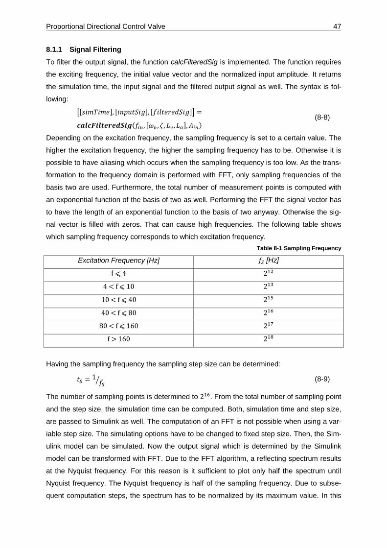
Proportional Directional Control Valve 47
8.1.1 Signal Filtering
To filter the output signal, the function calcFilteredSig is implemented. The function requires
the exciting frequency, the initial value vector and the normalized input amplitude. It returns
the simulation time, the input signal and the filtered output signal as well. The syntax is fol-
lowing:
[[𝑠𝑖𝑚𝑇𝑖𝑚𝑒], [𝑖𝑛𝑝𝑢𝑡𝑆𝑖𝑔], [𝑓𝑖𝑙𝑡𝑒𝑟𝑒𝑑𝑆𝑖𝑔]] =
𝒄𝒂𝒍𝒄𝑭𝒊𝒍𝒕𝒆𝒓𝒆𝒅𝑺𝒊𝒈(𝑓𝑖𝑛, [𝜔𝑛, 𝜁, 𝐿𝑣 , 𝐿𝑎], 𝐴𝑖𝑛) (8-8)
Depending on the excitation frequency, the sampling frequency is set to a certain value. The
higher the excitation frequency, the higher the sampling frequency has to be. Otherwise it is
possible to have aliasing which occurs when the sampling frequency is too low. As the trans-
formation to the frequency domain is performed with FFT, only sampling frequencies of the
basis two are used. Furthermore, the total number of measurement points is computed with
an exponential function of the basis of two as well. Performing the FFT the signal vector has
to have the length of an exponential function to the basis of two anyway. Otherwise the sig-
nal vector is filled with zeros. That can cause high frequencies. The following table shows
which sampling frequency corresponds to which excitation frequency.
Table 8-1 Sampling Frequency
Excitation Frequency [Hz] 𝑓𝑆 [Hz]
f ⩽ 4 212
4 < f ⩽ 10 213
10 < f ⩽ 40 215
40 < f ⩽ 80 216
80 < f ⩽ 160 217
f > 160 218
Having the sampling frequency the sampling step size can be determined:
𝑡𝑆 =1𝑓𝑆⁄ (8-9)
The number of sampling points is determined to 216. From the total number of sampling point
and the step size, the simulation time can be computed. Both, simulation time and step size,
are passed to Simulink as well. The computation of an FFT is not possible when using a var-
iable step size. The simulating options have to be changed to fixed step size. Then, the Sim-
ulink model can be simulated. Now the output signal which is determined by the Simulink
model can be transformed with FFT. Due to the FFT algorithm, a reflecting spectrum results
at the Nyquist frequency. For this reason is it sufficient to plot only half the spectrum until
Nyquist frequency. The Nyquist frequency is half of the sampling frequency. Due to subse-
quent computation steps, the spectrum has to be normalized by its maximum value. In this
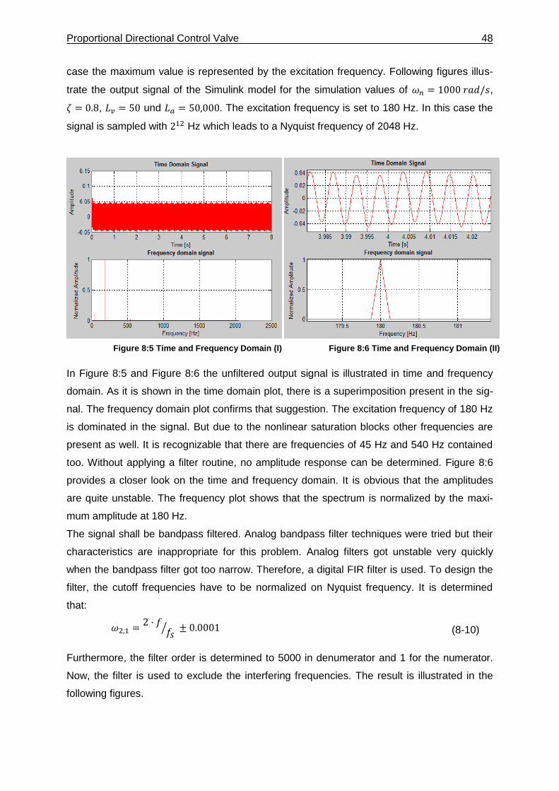
Proportional Directional Control Valve 48
case the maximum value is represented by the excitation frequency. Following figures illus-
trate the output signal of the Simulink model for the simulation values of 𝜔𝑛 = 1000 𝑟𝑎𝑑/𝑠,
𝜁 = 0.8, 𝐿𝑣 = 50 und 𝐿𝑎 = 50,000. The excitation frequency is set to 180 Hz. In this case the
signal is sampled with 212 Hz which leads to a Nyquist frequency of 2048 Hz.
In Figure 8:5 and Figure 8:6 the unfiltered output signal is illustrated in time and frequency
domain. As it is shown in the time domain plot, there is a superimposition present in the sig-
nal. The frequency domain plot confirms that suggestion. The excitation frequency of 180 Hz
is dominated in the signal. But due to the nonlinear saturation blocks other frequencies are
present as well. It is recognizable that there are frequencies of 45 Hz and 540 Hz contained
too. Without applying a filter routine, no amplitude response can be determined. Figure 8:6
provides a closer look on the time and frequency domain. It is obvious that the amplitudes
are quite unstable. The frequency plot shows that the spectrum is normalized by the maxi-
mum amplitude at 180 Hz.
The signal shall be bandpass filtered. Analog bandpass filter techniques were tried but their
characteristics are inappropriate for this problem. Analog filters got unstable very quickly
when the bandpass filter got too narrow. Therefore, a digital FIR filter is used. To design the
filter, the cutoff frequencies have to be normalized on Nyquist frequency. It is determined
that:
𝜔2,1 =2 · 𝑓
𝑓𝑆⁄ ± 0.0001 (8-10)
Furthermore, the filter order is determined to 5000 in denumerator and 1 for the numerator.
Now, the filter is used to exclude the interfering frequencies. The result is illustrated in the
following figures.
Figure 8:5 Time and Frequency Domain (I) Figure 8:6 Time and Frequency Domain (II)
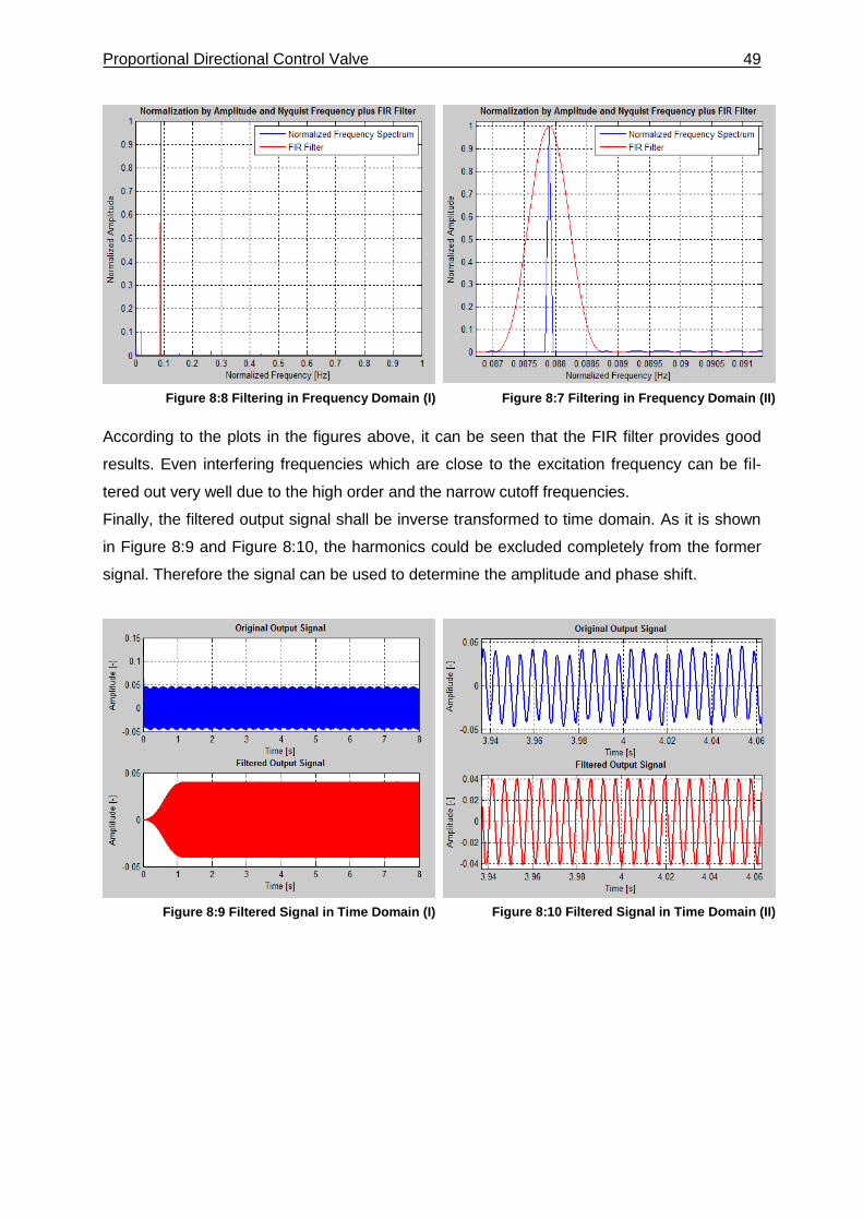
Proportional Directional Control Valve 49
According to the plots in the figures above, it can be seen that the FIR filter provides good
results. Even interfering frequencies which are close to the excitation frequency can be fil-
tered out very well due to the high order and the narrow cutoff frequencies.
Finally, the filtered output signal shall be inverse transformed to time domain. As it is shown
in Figure 8:9 and Figure 8:10, the harmonics could be excluded completely from the former
signal. Therefore the signal can be used to determine the amplitude and phase shift.
Figure 8:8 Filtering in Frequency Domain (I) Figure 8:7 Filtering in Frequency Domain (II)
Figure 8:9 Filtered Signal in Time Domain (I) Figure 8:10 Filtered Signal in Time Domain (II)
Proportional Directional Control Valve 50
8.1.2 Finding Intersection
To determine amplitude and phase response, the output signal has to be analyzed precisely.
The amplitude response can only be computed when steady oscillation behavior is reached.
That is explained in detail in section 2.4. Now the objective is to determine the intersections
of the output signal. Between these intersections positive and negative half-waves are locat-
ed. The half-waves necessarily contain amplitudes. When the amplitudes and areas under-
neath the curve of two consecutive half-waves are nearly the same, steady oscillation is
reached. For this reason the intersections are important for integration limits. Furthermore,
they are needed to compute the phase shift between output and input signal.
A function has been created to detect all time steps in which a zero-crossing occurs in the
signal. Therefore the signal value vector and the time vector have to pass to the function.
The syntax is described below.
[[𝑣𝑒𝑐𝑍𝑒𝑟𝑜], [𝑣𝑒𝑐𝑍𝑒𝑟𝑜𝑃𝑜𝑠], [𝑣𝑒𝑐𝑍𝑒𝑟𝑜𝑁𝑒𝑔], [𝑡𝑍𝑒𝑟𝑜𝑃𝑜𝑠], [𝑡𝑍𝑒𝑟𝑜𝑁𝑒𝑔]] =
𝒄𝒂𝒍𝒄𝒁𝒆𝒓𝒐𝑪𝒓𝒐𝒔𝒔𝒊𝒏𝒈𝒔([𝑠𝑖𝑔𝑛𝑎𝑙 𝑣𝑎𝑙𝑢𝑒𝑠], [𝑡𝑖𝑚𝑒])
(8-11)
With: · 𝑣𝑒𝑐𝑍𝑒𝑟𝑜 ⟶ Vector with all intersection
· 𝑣𝑒𝑐𝑍𝑒𝑟𝑜𝑃𝑜𝑠 ⟶ Vector with only positive intersections
· 𝑣𝑒𝑐𝑍𝑒𝑟𝑜𝑁𝑒𝑔 ⟶ Vector with only negative intersections
· 𝑡𝑍𝑒𝑟𝑜𝑃𝑜𝑠 ⟶ Time span vector for positive intersections
· 𝑡𝑍𝑒𝑟𝑜𝑁𝑒𝑔 ⟶ Time span vector for negative intersections
The zero-crossings of a signal can be described in two different ways. Before the signal is
intersecting the x-axis it can be positive or negative. Therefore, the terms ‘positive zero-
crossing’ and ‘negative zero-crossing’ shall be introduced. When the signal intersects from
positive to negative, a positive zero-crossing can be detected. When the function has a nega-
tive value before intersecting the x-axis, a negative zero-crossing can be detected. This is
illustrated in Figure 8:11 below.
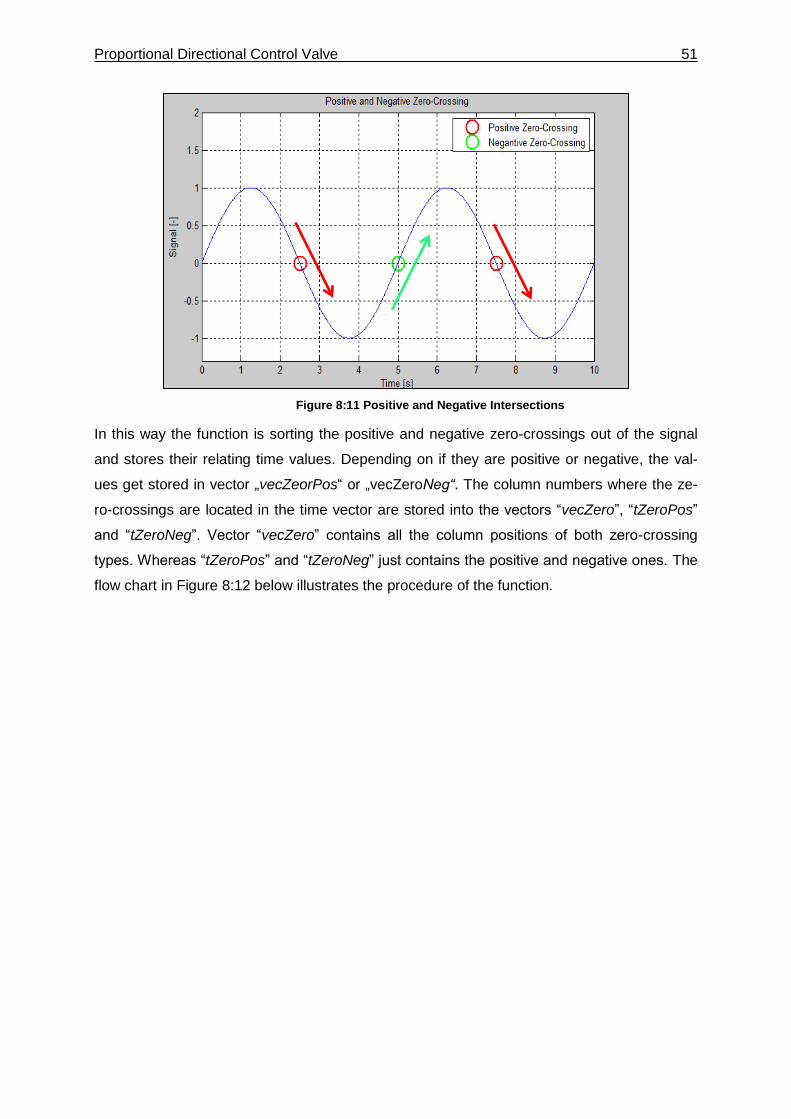
Proportional Directional Control Valve 51
Figure 8:11 Positive and Negative Intersections
In this way the function is sorting the positive and negative zero-crossings out of the signal
and stores their relating time values. Depending on if they are positive or negative, the val-
ues get stored in vector „vecZeorPos“ or „vecZeroNeg“. The column numbers where the ze-
ro-crossings are located in the time vector are stored into the vectors “vecZero”, “tZeroPos”
and “tZeroNeg”. Vector “vecZero” contains all the column positions of both zero-crossing
types. Whereas “tZeroPos” and “tZeroNeg” just contains the positive and negative ones. The
flow chart in Figure 8:12 below illustrates the procedure of the function.
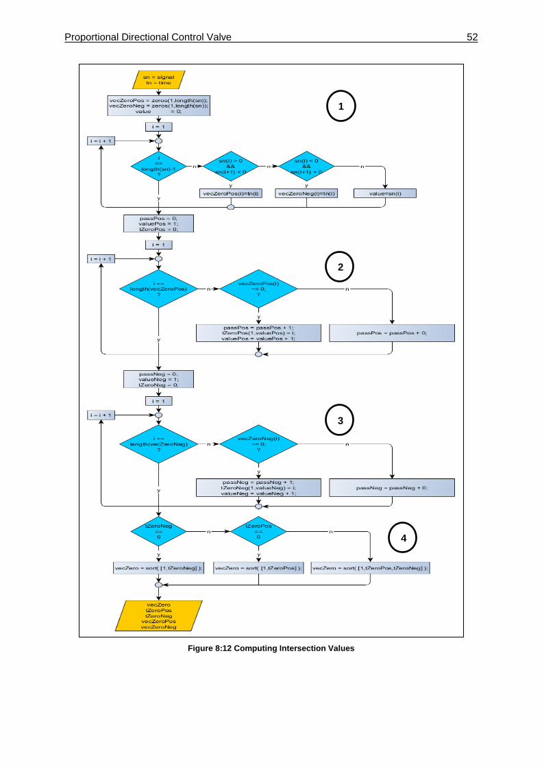
Proportional Directional Control Valve 52
Figure 8:12 Computing Intersection Values
1
2
3
4
Proportional Directional Control Valve 53
At first it has to be looped through signal vector, checking at any position if the current value
is bigger than zero and if the following is less than zero. If so, it detects a positive zero-
crossing and adds this time to the vector vecZeroPos. The same procedure is applied for
negative zero-crossing with switched operators (①).
Then, it has to be checked how many positive and negative zero-crossings occurred. Total
number of both get detected and stored in passPos respectively passNeg. Then the function
loops through the vector vecZeroPos and checks if the current value is not equal to zero. If
so, the value gets stored in vector tZeroPos otherwise the counter increases (②).
To determine the negative zero-crossing, the same procedure as it is described in ② has to
be applied. The positions get stored in tZeroNeg (③).
Finally, the all zero-crossings get stored in one vector one after another (④).
8.1.3 Determining Zero-Matrixes
Building up zero-matrixes is important because Matlab does not fill up an array with an in-
consistent number of vectors by itself. But especially in the beginning, when the natural fre-
quency interferes with the excitation frequency, the resulting frequency can vary. That means
one period in the beginning can have more discrete measured data points. This is why the
length of the different vectors for all the half-waves is going to be different as well. To bring
them all together a zero matrix is needed. The calcZeroMatrixes function has the task of pro-
ducing zero matrixes for the positive and negative half-waves. They were designated as
posMat and negMat. Therefore, it has to be known at which time point a zero-crossing oc-
curs and how many positive and negative half-waves are contained in the signal. For this
reason calcZeroMatrixes also uses the outputs from calcZeroCrossings which is described in
the previous section.
[[𝑝𝑜𝑠𝑀𝑎𝑡], [𝑛𝑒𝑔𝑀𝑎𝑡], [𝑙𝑀𝑎𝑡], [𝑙]] =
𝒄𝒂𝒍𝒄𝒁𝒆𝒓𝒐𝑴𝒂𝒕𝒓𝒊𝒙𝒆𝒔(𝑠𝑤𝑖𝑡𝑐ℎ𝑒𝑟, [𝑣𝑒𝑐𝑍𝑒𝑟𝑜]) (8-12)
With: · 𝑝𝑜𝑠𝑀𝑎𝑡 ⟶ Zero matrix for positive half-waves
· 𝑛𝑒𝑔𝑀𝑎𝑡 ⟶ Zero matrix for negative half-waves
· 𝑙𝑀𝑎𝑡 ⟶ Row dimension of posMat and negMat
· 𝑙 ⟶ Time span vector for positive intersections
· 𝑠𝑤𝑖𝑡𝑐ℎ𝑒𝑟 ⟶ Boolean value which indicates if the first value in the signal is posi-
tive (1) or negative (0)
· 𝑣𝑒𝑐𝑍𝑒𝑟𝑜 ⟶ Vector with all intersection
The column number of the zero matrix has to have the same length as the number of data
points measured for the longest half-period. The number of rows depends on the number of
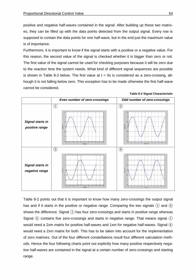
Proportional Directional Control Valve 54
positive and negative half-waves contained in the signal. After building up these two matrix-
es, they can be filled up with the data points detected from the output signal. Every row is
supposed to contain the data points for one half-wave, but in the end just the maximum value
is of importance.
Furthermore, it is important to know if the signal starts with a positive or a negative value. For
this reason, the second value of the signal is checked whether it is bigger than zero or not.
The first value of the signal cannot be used for checking purposes because it will be zero due
to the reaction time the system needs. What kind of different signal sequences are possible
is shown in Table 8-2 below. The first value at t = 0s is considered as a zero-crossing, alt-
hough it is not falling below zero. This exception has to be made otherwise the first half-wave
cannot be considered.
Table 8-2 Signal Characteristic
Even number of zero-crossings Odd number of zero-crossings
Signal starts in
positive range
①
②
Signal starts in
negative range
③
④
Table 8-2 points out that it is important to know how many zero-crossings the output signal
has and if it starts in the positive or negative range. Comparing the two signals ① and ④
shows the difference. Signal ① has four zero-crossings and starts in positive range whereas
Signal ④ contains five zero-crossings and starts in negative range. That means signal ①
would need a 2xm matrix for positive half-waves and 1xm for negative half-waves. Signal ④
would need a 2xm matrix for both. This has to be taken into account for the implementation
of zero matrixes. Out of the four different constellations result four different calculation meth-
ods. Hence the four following charts point out explicitly how many positive respectively nega-
tive half-waves are contained in the signal at a certain number of zero-crossings and starting
range.
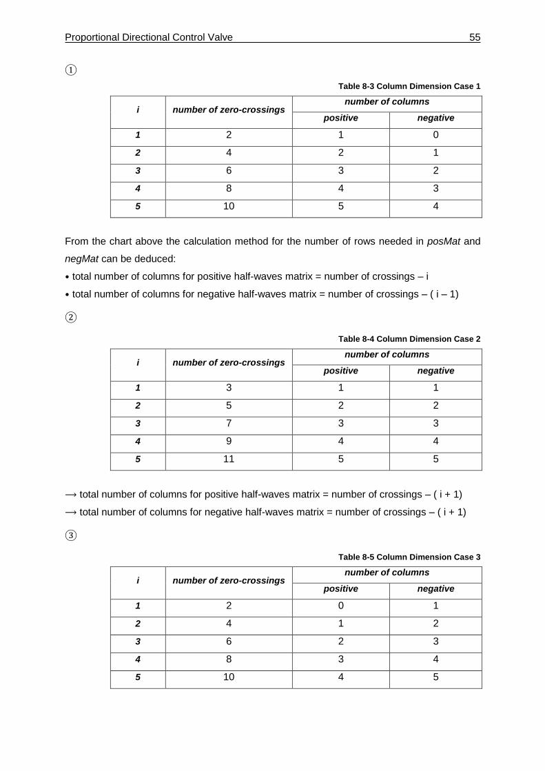
Proportional Directional Control Valve 55
①
Table 8-3 Column Dimension Case 1
i number of zero-crossings number of columns
positive negative
1 2 1 0
2 4 2 1
3 6 3 2
4 8 4 3
5 10 5 4
From the chart above the calculation method for the number of rows needed in posMat and
negMat can be deduced:
• total number of columns for positive half-waves matrix = number of crossings – i
• total number of columns for negative half-waves matrix = number of crossings – ( i – 1)
②
Table 8-4 Column Dimension Case 2
i number of zero-crossings number of columns
positive negative
1 3 1 1
2 5 2 2
3 7 3 3
4 9 4 4
5 11 5 5
⟶ total number of columns for positive half-waves matrix = number of crossings – ( i + 1)
⟶ total number of columns for negative half-waves matrix = number of crossings – ( i + 1)
③
Table 8-5 Column Dimension Case 3
i number of zero-crossings number of columns
positive negative
1 2 0 1
2 4 1 2
3 6 2 3
4 8 3 4
5 10 4 5
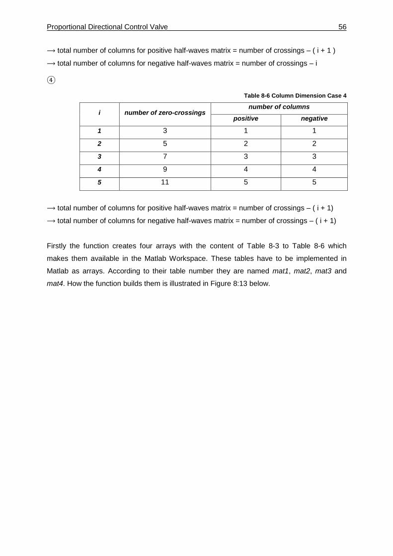
Proportional Directional Control Valve 56
⟶ total number of columns for positive half-waves matrix = number of crossings – ( i + 1 )
⟶ total number of columns for negative half-waves matrix = number of crossings – i
④
Table 8-6 Column Dimension Case 4
i number of zero-crossings number of columns
positive negative
1 3 1 1
2 5 2 2
3 7 3 3
4 9 4 4
5 11 5 5
⟶ total number of columns for positive half-waves matrix = number of crossings – ( i + 1)
⟶ total number of columns for negative half-waves matrix = number of crossings – ( i + 1)
Firstly the function creates four arrays with the content of Table 8-3 to Table 8-6 which
makes them available in the Matlab Workspace. These tables have to be implemented in
Matlab as arrays. According to their table number they are named mat1, mat2, mat3 and
mat4. How the function builds them is illustrated in Figure 8:13 below.
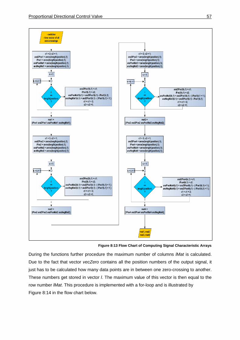
Proportional Directional Control Valve 57
Figure 8:13 Flow Chart of Computing Signal Characteristic Arrays
During the functions further procedure the maximum number of columns lMat is calculated.
Due to the fact that vector vecZero contains all the position numbers of the output signal, it
just has to be calculated how many data points are in between one zero-crossing to another.
These numbers get stored in vector l. The maximum value of this vector is then equal to the
row number lMat. This procedure is implemented with a for-loop and is illustrated by
Figure 8:14 in the flow chart below.
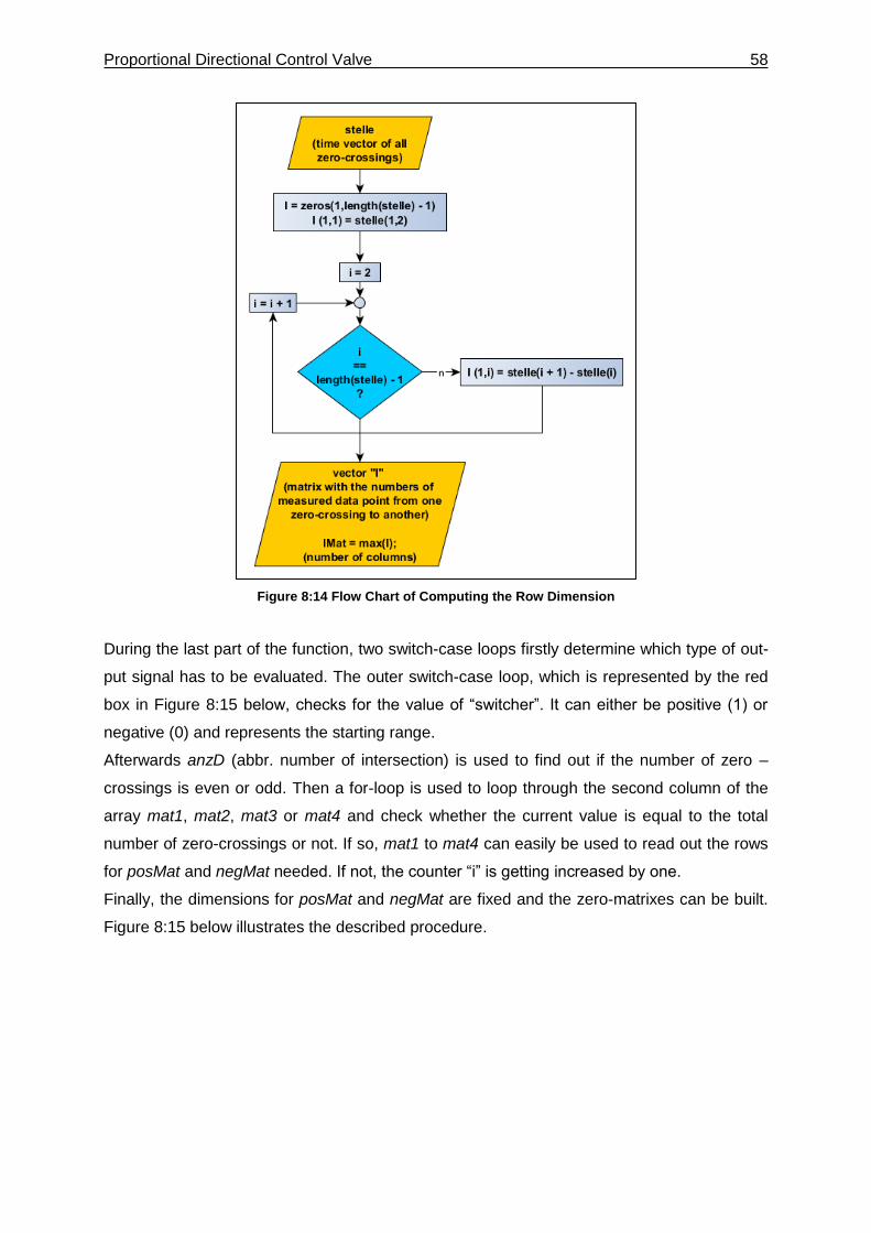
Proportional Directional Control Valve 58
Figure 8:14 Flow Chart of Computing the Row Dimension
During the last part of the function, two switch-case loops firstly determine which type of out-
put signal has to be evaluated. The outer switch-case loop, which is represented by the red
box in Figure 8:15 below, checks for the value of “switcher”. It can either be positive (1) or
negative (0) and represents the starting range.
Afterwards anzD (abbr. number of intersection) is used to find out if the number of zero –
crossings is even or odd. Then a for-loop is used to loop through the second column of the
array mat1, mat2, mat3 or mat4 and check whether the current value is equal to the total
number of zero-crossings or not. If so, mat1 to mat4 can easily be used to read out the rows
for posMat and negMat needed. If not, the counter “i” is getting increased by one.
Finally, the dimensions for posMat and negMat are fixed and the zero-matrixes can be built.
Figure 8:15 below illustrates the described procedure.
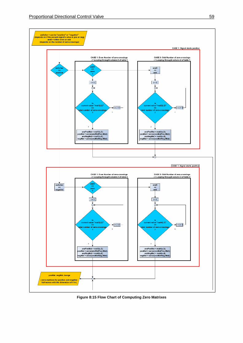
Proportional Directional Control Valve 59
Figure 8:15 Flow Chart of Computing Zero Matrixes
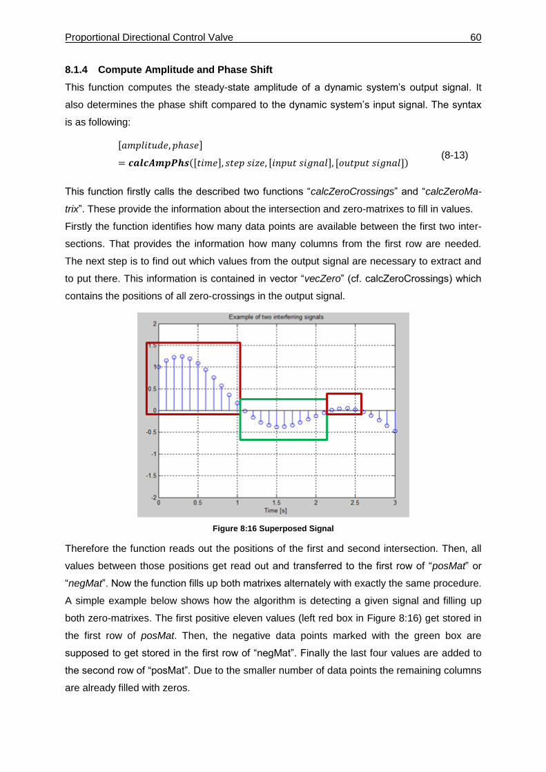
Proportional Directional Control Valve 60
8.1.4 Compute Amplitude and Phase Shift
This function computes the steady-state amplitude of a dynamic system’s output signal. It
also determines the phase shift compared to the dynamic system’s input signal. The syntax
is as following:
[𝑎𝑚𝑝𝑙𝑖𝑡𝑢𝑑𝑒, 𝑝ℎ𝑎𝑠𝑒]
= 𝒄𝒂𝒍𝒄𝑨𝒎𝒑𝑷𝒉𝒔([𝑡𝑖𝑚𝑒], 𝑠𝑡𝑒𝑝 𝑠𝑖𝑧𝑒, [𝑖𝑛𝑝𝑢𝑡 𝑠𝑖𝑔𝑛𝑎𝑙], [𝑜𝑢𝑡𝑝𝑢𝑡 𝑠𝑖𝑔𝑛𝑎𝑙]) (8-13)
This function firstly calls the described two functions “calcZeroCrossings” and “calcZeroMa-
trix”. These provide the information about the intersection and zero-matrixes to fill in values.
Firstly the function identifies how many data points are available between the first two inter-
sections. That provides the information how many columns from the first row are needed.
The next step is to find out which values from the output signal are necessary to extract and
to put there. This information is contained in vector “vecZero” (cf. calcZeroCrossings) which
contains the positions of all zero-crossings in the output signal.
Figure 8:16 Superposed Signal
Therefore the function reads out the positions of the first and second intersection. Then, all
values between those positions get read out and transferred to the first row of “posMat” or
“negMat”. Now the function fills up both matrixes alternately with exactly the same procedure.
A simple example below shows how the algorithm is detecting a given signal and filling up
both zero-matrixes. The first positive eleven values (left red box in Figure 8:16) get stored in
the first row of posMat. Then, the negative data points marked with the green box are
supposed to get stored in the first row of “negMat”. Finally the last four values are added to
the second row of “posMat”. Due to the smaller number of data points the remaining columns
are already filled with zeros.
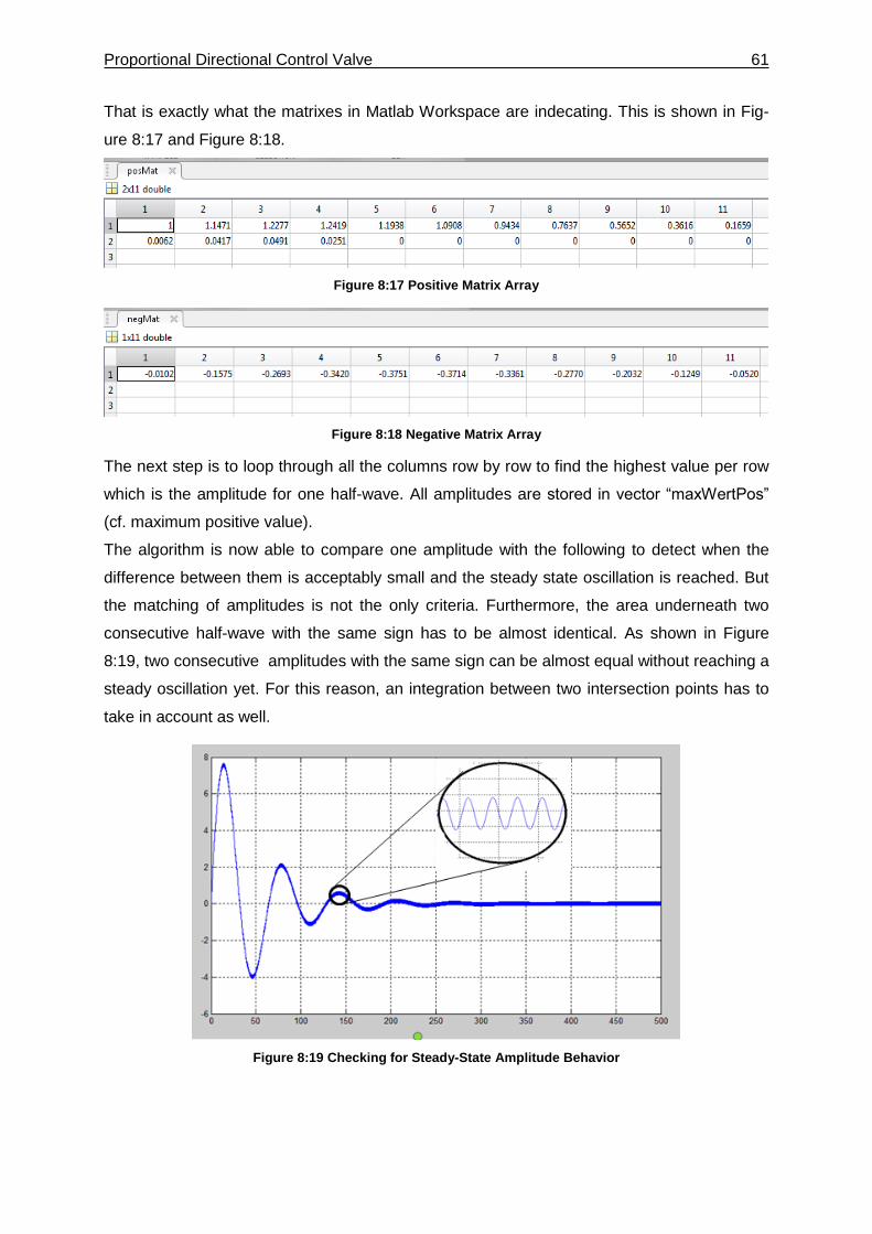
Proportional Directional Control Valve 61
That is exactly what the matrixes in Matlab Workspace are indecating. This is shown in Fig-
ure 8:17 and Figure 8:18.
Figure 8:17 Positive Matrix Array
Figure 8:18 Negative Matrix Array
The next step is to loop through all the columns row by row to find the highest value per row
which is the amplitude for one half-wave. All amplitudes are stored in vector “maxWertPos”
(cf. maximum positive value).
The algorithm is now able to compare one amplitude with the following to detect when the
difference between them is acceptably small and the steady state oscillation is reached. But
the matching of amplitudes is not the only criteria. Furthermore, the area underneath two
consecutive half-wave with the same sign has to be almost identical. As shown in Figure
8:19, two consecutive amplitudes with the same sign can be almost equal without reaching a
steady oscillation yet. For this reason, an integration between two intersection points has to
take in account as well.
Figure 8:19 Checking for Steady-State Amplitude Behavior
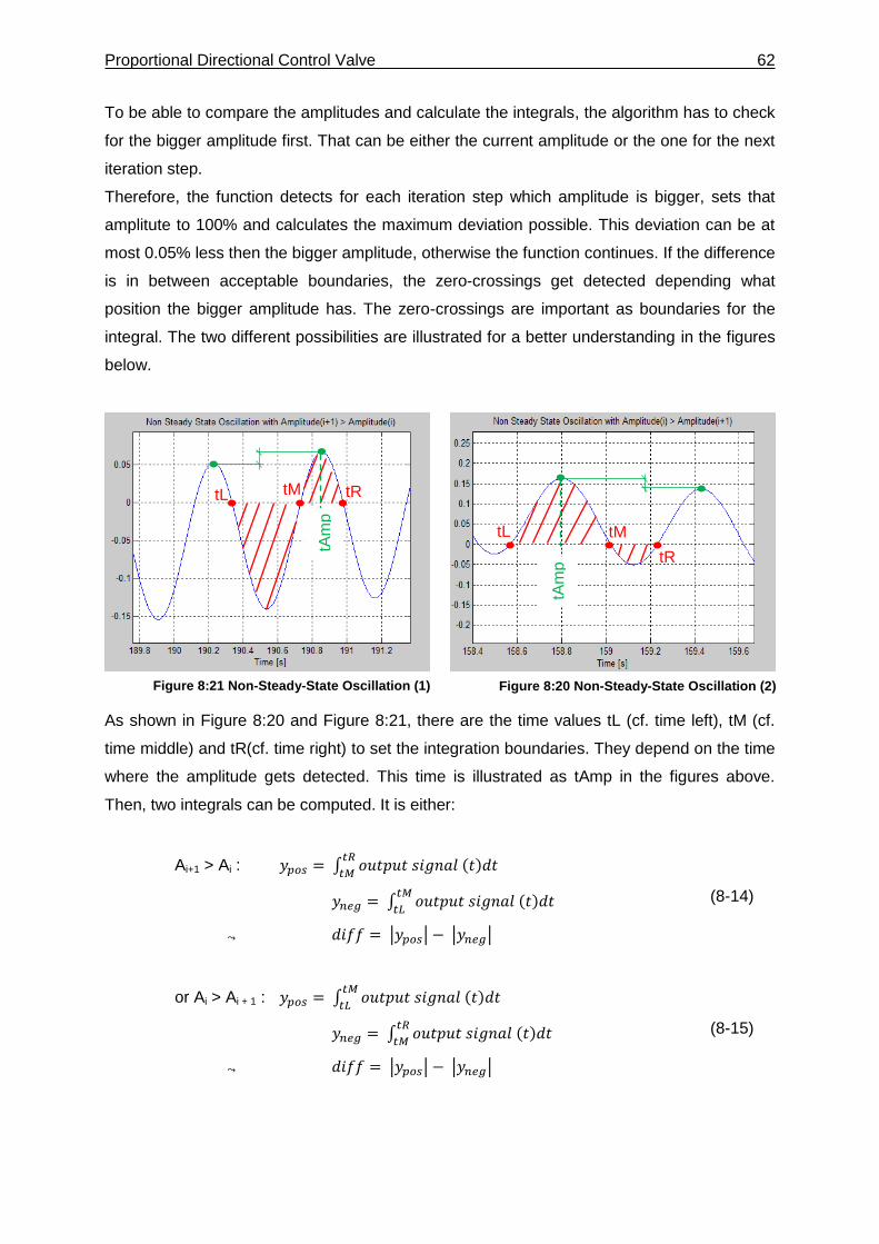
Proportional Directional Control Valve 62
To be able to compare the amplitudes and calculate the integrals, the algorithm has to check
for the bigger amplitude first. That can be either the current amplitude or the one for the next
iteration step.
Therefore, the function detects for each iteration step which amplitude is bigger, sets that
amplitute to 100% and calculates the maximum deviation possible. This deviation can be at
most 0.05% less then the bigger amplitude, otherwise the function continues. If the difference
is in between acceptable boundaries, the zero-crossings get detected depending what
position the bigger amplitude has. The zero-crossings are important as boundaries for the
integral. The two different possibilities are illustrated for a better understanding in the figures
below.
As shown in Figure 8:20 and Figure 8:21, there are the time values tL (cf. time left), tM (cf.
time middle) and tR(cf. time right) to set the integration boundaries. They depend on the time
where the amplitude gets detected. This time is illustrated as tAmp in the figures above.
Then, two integrals can be computed. It is either:
Ai+1 > Ai : 𝑦𝑝𝑜𝑠 = ∫ 𝑜𝑢𝑡𝑝𝑢𝑡 𝑠𝑖𝑔𝑛𝑎𝑙 (𝑡)𝑑𝑡𝑡𝑅
𝑡𝑀
𝑦𝑛𝑒𝑔 = ∫ 𝑜𝑢𝑡𝑝𝑢𝑡 𝑠𝑖𝑔𝑛𝑎𝑙 (𝑡)𝑑𝑡𝑡𝑀
𝑡𝐿
⤳ 𝑑𝑖𝑓𝑓 = |𝑦𝑝𝑜𝑠| − |𝑦𝑛𝑒𝑔|
(8-14)
or Ai > Ai + 1 : 𝑦𝑝𝑜𝑠 = ∫ 𝑜𝑢𝑡𝑝𝑢𝑡 𝑠𝑖𝑔𝑛𝑎𝑙 (𝑡)𝑑𝑡𝑡𝑀
𝑡𝐿
𝑦𝑛𝑒𝑔 = ∫ 𝑜𝑢𝑡𝑝𝑢𝑡 𝑠𝑖𝑔𝑛𝑎𝑙 (𝑡)𝑑𝑡𝑡𝑅
𝑡𝑀
⤳ 𝑑𝑖𝑓𝑓 = |𝑦𝑝𝑜𝑠| − |𝑦𝑛𝑒𝑔|
(8-15)
tL tM
tR
tL tM tR
tAm
p
tAm
p
Figure 8:20 Non-Steady-State Oscillation (2) Figure 8:21 Non-Steady-State Oscillation (1)
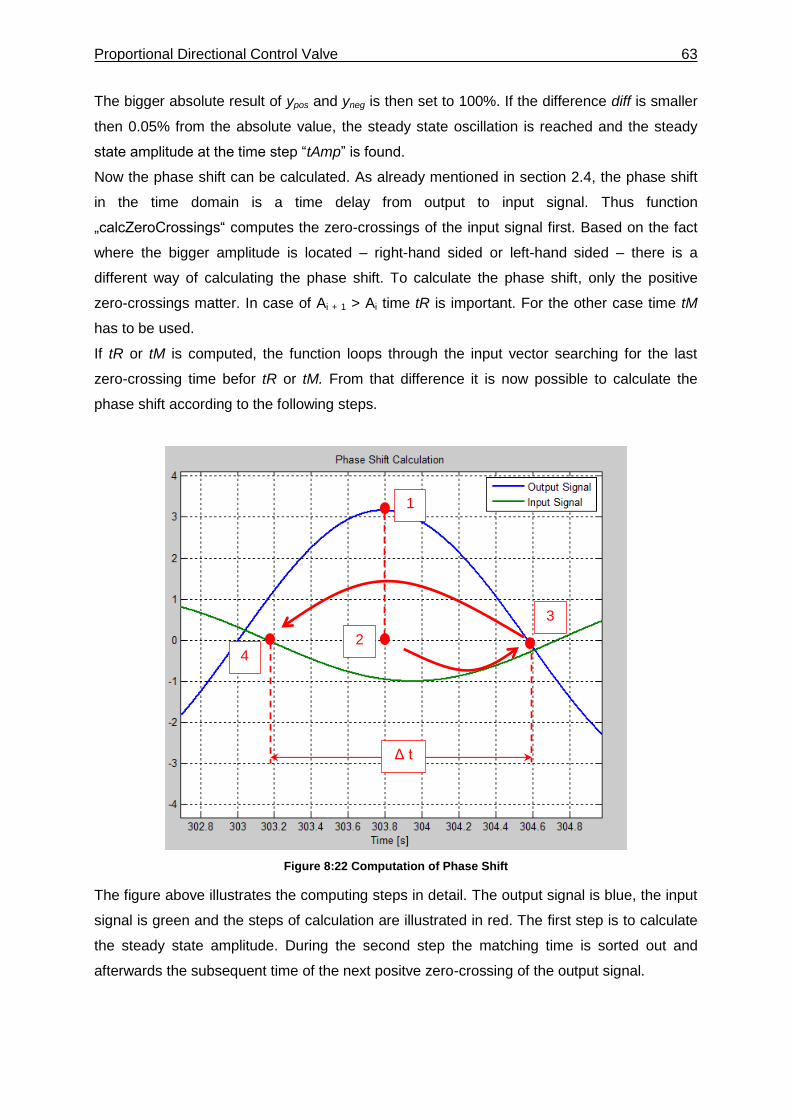
Proportional Directional Control Valve 63
The bigger absolute result of ypos and yneg is then set to 100%. If the difference diff is smaller
then 0.05% from the absolute value, the steady state oscillation is reached and the steady
state amplitude at the time step “tAmp” is found.
Now the phase shift can be calculated. As already mentioned in section 2.4, the phase shift
in the time domain is a time delay from output to input signal. Thus function
„calcZeroCrossings“ computes the zero-crossings of the input signal first. Based on the fact
where the bigger amplitude is located – right-hand sided or left-hand sided – there is a
different way of calculating the phase shift. To calculate the phase shift, only the positive
zero-crossings matter. In case of Ai + 1 > Ai time tR is important. For the other case time tM
has to be used.
If tR or tM is computed, the function loops through the input vector searching for the last
zero-crossing time befor tR or tM. From that difference it is now possible to calculate the
phase shift according to the following steps.
Figure 8:22 Computation of Phase Shift
The figure above illustrates the computing steps in detail. The output signal is blue, the input
signal is green and the steps of calculation are illustrated in red. The first step is to calculate
the steady state amplitude. During the second step the matching time is sorted out and
afterwards the subsequent time of the next positve zero-crossing of the output signal.
1
2
3
4
Δ t
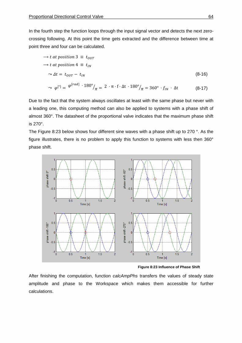
Proportional Directional Control Valve 64
In the fourth step the function loops through the input signal vector and detects the next zero-
crossing following. At this point the time gets extracted and the difference between time at
point three and four can be calculated.
⟶ 𝑡 𝑎𝑡 𝑝𝑜𝑠𝑖𝑡𝑖𝑜𝑛 3 ≡ 𝑡𝑂𝑈𝑇
⟶ 𝑡 𝑎𝑡 𝑝𝑜𝑠𝑖𝑡𝑖𝑜𝑛 4 ≡ 𝑡𝐼𝑁
⤳ 𝛥𝑡 = 𝑡𝑂𝑈𝑇 − 𝑡𝐼𝑁 (8-16)
⤳ 𝜑[°] = 𝜑[𝑟𝑎𝑑] · 180°
𝜋⁄ = 2 · π · f · Δt · 180° 𝜋⁄ = 360° · 𝑓𝐼𝑁 · Δt (8-17)
Due to the fact that the system always oscillates at least with the same phase but never with
a leading one, this computing method can also be applied to systems with a phase shift of
almost 360°. The datasheet of the proportional valve indicates that the maximum phase shift
is 270°.
The Figure 8:23 below shows four different sine waves with a phase shift up to 270 °. As the
figure illustrates, there is no problem to apply this function to systems with less then 360°
phase shift.
Figure 8:23 Influence of Phase Shift
After finishing the computation, function calcAmpPhs transfers the values of steady state
amplitude and phase to the Workspace which makes them accessible for further
calculations.
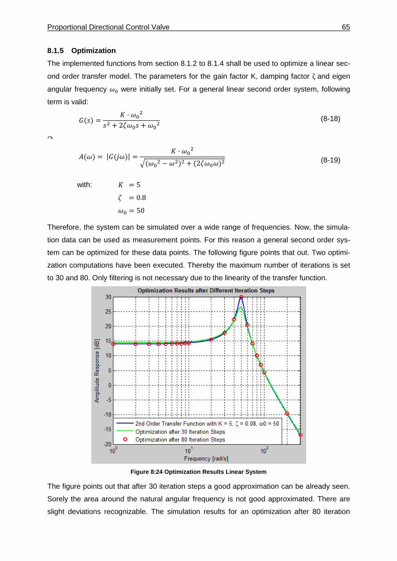
Proportional Directional Control Valve 65
8.1.5 Optimization
The implemented functions from section 8.1.2 to 8.1.4 shall be used to optimize a linear sec-
ond order transfer model. The parameters for the gain factor K, damping factor ζ and eigen
angular frequency 𝜔0 were initially set. For a general linear second order system, following
term is valid:
𝐺(𝑠) =𝐾 · 𝜔0
2
𝑠2 + 2𝜁𝜔0𝑠 + 𝜔02 (8-18)
↷
𝐴(𝜔) = |𝐺(𝑗𝜔)| =
𝐾 · 𝜔02
√(𝜔02 −𝜔2)2 + (2𝜁𝜔0𝜔)
2
(8-19)
with: 𝐾 = 5
𝜁 = 0.8
𝜔0 = 50
Therefore, the system can be simulated over a wide range of frequencies. Now, the simula-
tion data can be used as measurement points. For this reason a general second order sys-
tem can be optimized for these data points. The following figure points that out. Two optimi-
zation computations have been executed. Thereby the maximum number of iterations is set
to 30 and 80. Only filtering is not necessary due to the linearity of the transfer function.
Figure 8:24 Optimization Results Linear System
The figure points out that after 30 iteration steps a good approximation can be already seen.
Sorely the area around the natural angular frequency is not good approximated. There are
slight deviations recognizable. The simulation results for an optimization after 80 iteration
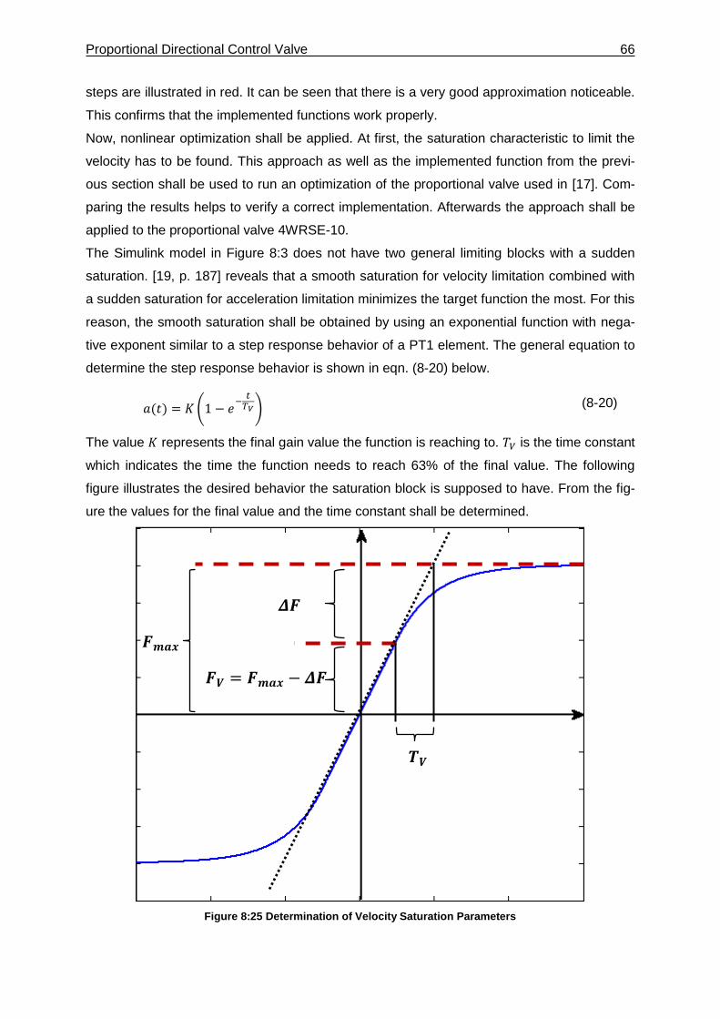
Proportional Directional Control Valve 66
steps are illustrated in red. It can be seen that there is a very good approximation noticeable.
This confirms that the implemented functions work properly.
Now, nonlinear optimization shall be applied. At first, the saturation characteristic to limit the
velocity has to be found. This approach as well as the implemented function from the previ-
ous section shall be used to run an optimization of the proportional valve used in [17]. Com-
paring the results helps to verify a correct implementation. Afterwards the approach shall be
applied to the proportional valve 4WRSE-10.
The Simulink model in Figure 8:3 does not have two general limiting blocks with a sudden
saturation. [19, p. 187] reveals that a smooth saturation for velocity limitation combined with
a sudden saturation for acceleration limitation minimizes the target function the most. For this
reason, the smooth saturation shall be obtained by using an exponential function with nega-
tive exponent similar to a step response behavior of a PT1 element. The general equation to
determine the step response behavior is shown in eqn. (8-20) below.
𝑎(𝑡) = 𝐾 (1 − 𝑒−𝑡𝑇𝑉) (8-20)
The value 𝐾 represents the final gain value the function is reaching to. 𝑇𝑉 is the time constant
which indicates the time the function needs to reach 63% of the final value. The following
figure illustrates the desired behavior the saturation block is supposed to have. From the fig-
ure the values for the final value and the time constant shall be determined.
Figure 8:25 Determination of Velocity Saturation Parameters
𝑭𝑽 = 𝑭𝒎𝒂𝒙 − 𝜟𝑭
𝜟𝑭
𝑻𝑽
𝑭𝒎𝒂𝒙
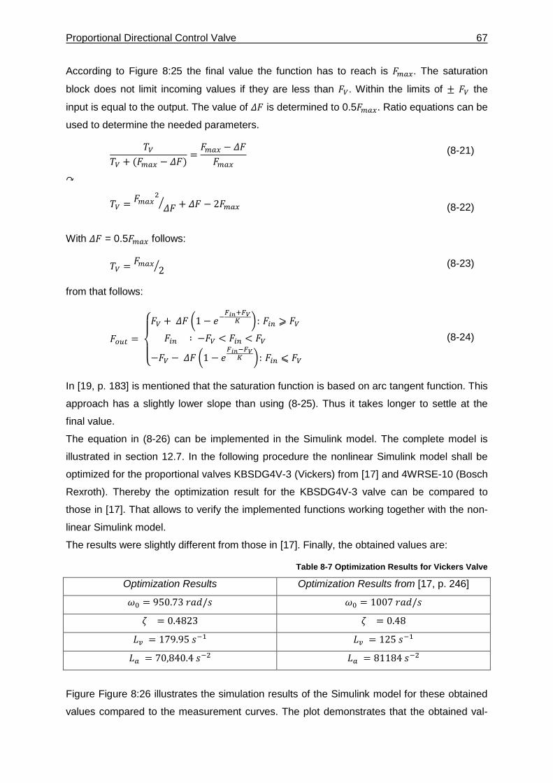
Proportional Directional Control Valve 67
According to Figure 8:25 the final value the function has to reach is 𝐹𝑚𝑎𝑥. The saturation
block does not limit incoming values if they are less than 𝐹𝑉. Within the limits of ± 𝐹𝑉 the
input is equal to the output. The value of 𝛥𝐹 is determined to 0.5𝐹𝑚𝑎𝑥. Ratio equations can be
used to determine the needed parameters.
𝑇𝑉
𝑇𝑉 + (𝐹𝑚𝑎𝑥 − 𝛥𝐹)=𝐹𝑚𝑎𝑥 − 𝛥𝐹
𝐹𝑚𝑎𝑥 (8-21)
↷
𝑇𝑉 =
𝐹𝑚𝑎𝑥2
𝛥𝐹⁄ + 𝛥𝐹 − 2𝐹𝑚𝑎𝑥 (8-22)
With 𝛥𝐹 = 0.5𝐹𝑚𝑎𝑥 follows:
𝑇𝑉 =𝐹𝑚𝑎𝑥
2⁄ (8-23)
from that follows:
𝐹𝑜𝑢𝑡 =
{
𝐹𝑉 + 𝛥𝐹 (1 − 𝑒
−𝐹𝑖𝑛+𝐹𝑉
𝐾 ): 𝐹𝑖𝑛 ⩾ 𝐹𝑉
𝐹𝑖𝑛 ∶ −𝐹𝑉 < 𝐹𝑖𝑛 < 𝐹𝑉
−𝐹𝑉 − 𝛥𝐹 (1 − 𝑒𝐹𝑖𝑛−𝐹𝑉
𝐾 ): 𝐹𝑖𝑛 ⩽ 𝐹𝑉
(8-24)
In [19, p. 183] is mentioned that the saturation function is based on arc tangent function. This
approach has a slightly lower slope than using (8-25). Thus it takes longer to settle at the
final value.
The equation in (8-26) can be implemented in the Simulink model. The complete model is
illustrated in section 12.7. In the following procedure the nonlinear Simulink model shall be
optimized for the proportional valves KBSDG4V-3 (Vickers) from [17] and 4WRSE-10 (Bosch
Rexroth). Thereby the optimization result for the KBSDG4V-3 valve can be compared to
those in [17]. That allows to verify the implemented functions working together with the non-
linear Simulink model.
The results were slightly different from those in [17]. Finally, the obtained values are:
Table 8-7 Optimization Results for Vickers Valve
Optimization Results Optimization Results from [17, p. 246]
𝜔0 = 950.73 𝑟𝑎𝑑/𝑠 𝜔0 = 1007 𝑟𝑎𝑑/𝑠
𝜁 = 0.4823 𝜁 = 0.48
𝐿𝑣 = 179.95 𝑠−1 𝐿𝑣 = 125 𝑠
−1
𝐿𝑎 = 70,840.4 𝑠−2 𝐿𝑎 = 81184 𝑠
−2
Figure Figure 8:26 illustrates the simulation results of the Simulink model for these obtained
values compared to the measurement curves. The plot demonstrates that the obtained val-
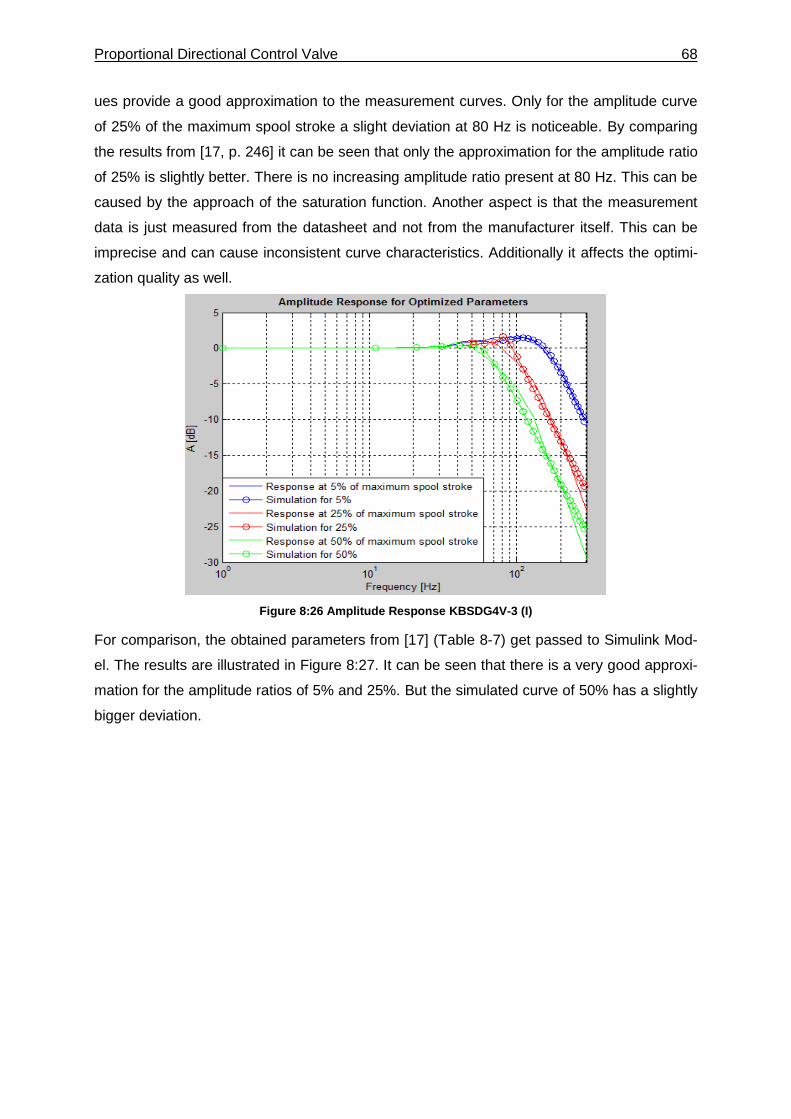
Proportional Directional Control Valve 68
ues provide a good approximation to the measurement curves. Only for the amplitude curve
of 25% of the maximum spool stroke a slight deviation at 80 Hz is noticeable. By comparing
the results from [17, p. 246] it can be seen that only the approximation for the amplitude ratio
of 25% is slightly better. There is no increasing amplitude ratio present at 80 Hz. This can be
caused by the approach of the saturation function. Another aspect is that the measurement
data is just measured from the datasheet and not from the manufacturer itself. This can be
imprecise and can cause inconsistent curve characteristics. Additionally it affects the optimi-
zation quality as well.
Figure 8:26 Amplitude Response KBSDG4V-3 (I)
For comparison, the obtained parameters from [17] (Table 8-7) get passed to Simulink Mod-
el. The results are illustrated in Figure 8:27. It can be seen that there is a very good approxi-
mation for the amplitude ratios of 5% and 25%. But the simulated curve of 50% has a slightly
bigger deviation.
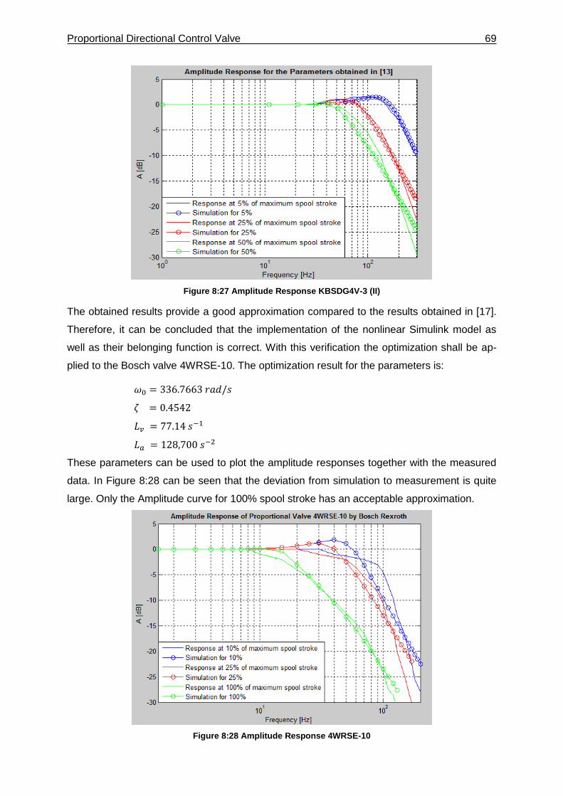
Proportional Directional Control Valve 69
Figure 8:27 Amplitude Response KBSDG4V-3 (II)
The obtained results provide a good approximation compared to the results obtained in [17].
Therefore, it can be concluded that the implementation of the nonlinear Simulink model as
well as their belonging function is correct. With this verification the optimization shall be ap-
plied to the Bosch valve 4WRSE-10. The optimization result for the parameters is:
𝜔0 = 336.7663 𝑟𝑎𝑑/𝑠
𝜁 = 0.4542
𝐿𝑣 = 77.14 𝑠−1
𝐿𝑎 = 128,700 𝑠−2
These parameters can be used to plot the amplitude responses together with the measured
data. In Figure 8:28 can be seen that the deviation from simulation to measurement is quite
large. Only the Amplitude curve for 100% spool stroke has an acceptable approximation.
Figure 8:28 Amplitude Response 4WRSE-10
Proportional Directional Control Valve 70
The target function stabilized at a value of 1020.38 which is 𝐹𝑡𝑎𝑟𝑔𝑒𝑡 = 1020.38 , being quite
large. For a good approximation the target function value is supposed to be between 5 and
40. Different sets of initial values have been tried to exclude local minimum solution. These
are shown in the following Table 8-8.
Table 8-8 Initial Values for Optimization of 4WRSE-10
𝜔0
[𝑟𝑎𝑑/𝑠]
𝜁
[−]
𝐿𝑣
[𝑠−1]
𝐿𝑎
[𝑠−2]
𝐴𝑏𝑜𝑟𝑡 𝐼𝑡𝑒𝑟𝑎𝑡𝑖𝑜𝑛
𝑎𝑡 𝑠𝑡𝑒𝑝
𝐹𝑡𝑎𝑟𝑔𝑒𝑡
[𝑥𝑖𝑛𝑖𝑡1] 900 0.5 100 90,000 140 1052
[𝑥𝑖𝑛𝑖𝑡2] 70 1 200 50,000 135 1073
[𝑥𝑖𝑛𝑖𝑡3] 625 900 70 10,000 142 1020.38
As Table 8-8 illustrates, the different sets of initial values lead all to the same result. The tar-
get function stabilizes at a value of around 1050.
The results for the proportional valve 4WRSE-10 are not as satisfying as those for
KBSDG4V-3. It can be assumed that the reason is the missing amplitude incensement. The
curves of 4WRSE-10 indicate that there is no excitation frequency where the output ampli-
tude gets amplified. The results for KBSDG4V-3 show that the implemented functions work
pretty well. In [19] several Simulink model approaches had to be tested to find an appropriate
model. A different approach for the Simulink model leads to better results more probably.
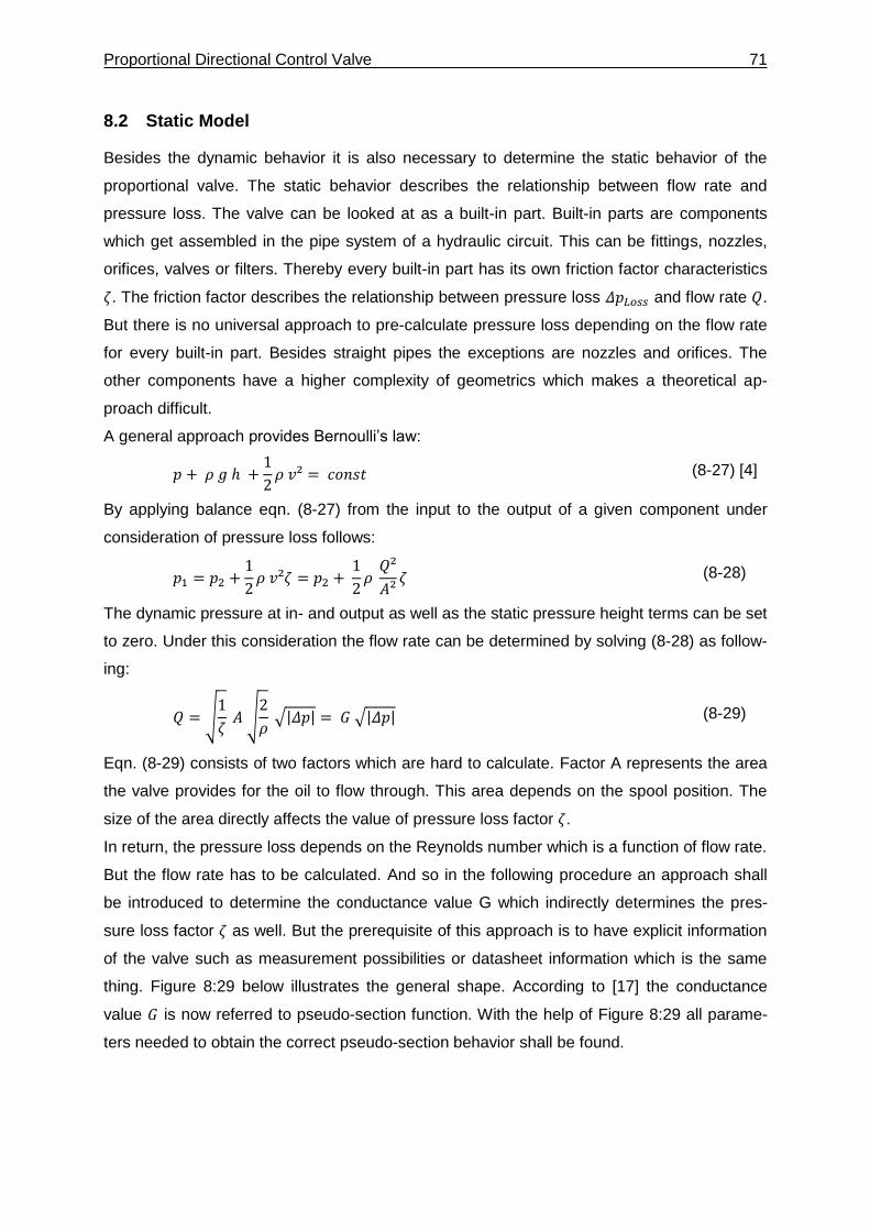
Proportional Directional Control Valve 71
8.2 Static Model
Besides the dynamic behavior it is also necessary to determine the static behavior of the
proportional valve. The static behavior describes the relationship between flow rate and
pressure loss. The valve can be looked at as a built-in part. Built-in parts are components
which get assembled in the pipe system of a hydraulic circuit. This can be fittings, nozzles,
orifices, valves or filters. Thereby every built-in part has its own friction factor characteristics
𝜁. The friction factor describes the relationship between pressure loss 𝛥𝑝𝐿𝑜𝑠𝑠 and flow rate 𝑄.
But there is no universal approach to pre-calculate pressure loss depending on the flow rate
for every built-in part. Besides straight pipes the exceptions are nozzles and orifices. The
other components have a higher complexity of geometrics which makes a theoretical ap-
proach difficult.
A general approach provides Bernoulli’s law:
𝑝 + 𝜌 𝑔 ℎ +1
2𝜌 𝑣² = 𝑐𝑜𝑛𝑠𝑡 (8-27) [4]
By applying balance eqn. (8-27) from the input to the output of a given component under
consideration of pressure loss follows:
𝑝1 = 𝑝2 +1
2𝜌 𝑣²𝜁 = 𝑝2 +
1
2𝜌 𝑄²
𝐴²𝜁 (8-28)
The dynamic pressure at in- and output as well as the static pressure height terms can be set
to zero. Under this consideration the flow rate can be determined by solving (8-28) as follow-
ing:
𝑄 = √1
𝜁 𝐴 √
2
𝜌 √|𝛥𝑝| = 𝐺 √|𝛥𝑝| (8-29)
Eqn. (8-29) consists of two factors which are hard to calculate. Factor A represents the area
the valve provides for the oil to flow through. This area depends on the spool position. The
size of the area directly affects the value of pressure loss factor 𝜁.
In return, the pressure loss depends on the Reynolds number which is a function of flow rate.
But the flow rate has to be calculated. And so in the following procedure an approach shall
be introduced to determine the conductance value G which indirectly determines the pres-
sure loss factor 𝜁 as well. But the prerequisite of this approach is to have explicit information
of the valve such as measurement possibilities or datasheet information which is the same
thing. Figure 8:29 below illustrates the general shape. According to [17] the conductance
value 𝐺 is now referred to pseudo-section function. With the help of Figure 8:29 all parame-
ters needed to obtain the correct pseudo-section behavior shall be found.
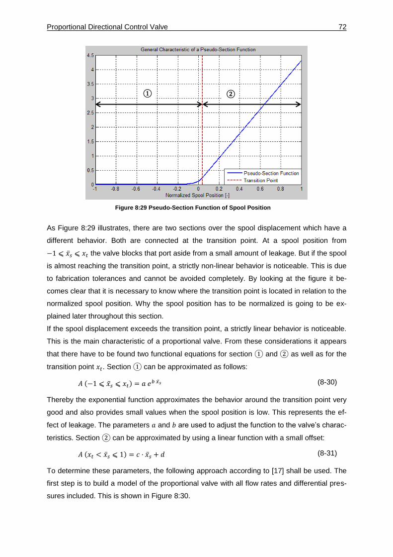
Proportional Directional Control Valve 72
Figure 8:29 Pseudo-Section Function of Spool Position
As Figure 8:29 illustrates, there are two sections over the spool displacement which have a
different behavior. Both are connected at the transition point. At a spool position from
−1 ⩽ �̅�𝑠 ⩽ 𝑥𝑡 the valve blocks that port aside from a small amount of leakage. But if the spool
is almost reaching the transition point, a strictly non-linear behavior is noticeable. This is due
to fabrication tolerances and cannot be avoided completely. By looking at the figure it be-
comes clear that it is necessary to know where the transition point is located in relation to the
normalized spool position. Why the spool position has to be normalized is going to be ex-
plained later throughout this section.
If the spool displacement exceeds the transition point, a strictly linear behavior is noticeable.
This is the main characteristic of a proportional valve. From these considerations it appears
that there have to be found two functional equations for section ① and ② as well as for the
transition point 𝑥𝑡. Section ① can be approximated as follows:
𝐴 (−1 ⩽ �̅�𝑠 ⩽ 𝑥𝑡) = 𝑎 𝑒𝑏 �̅�𝑠 (8-30)
Thereby the exponential function approximates the behavior around the transition point very
good and also provides small values when the spool position is low. This represents the ef-
fect of leakage. The parameters 𝑎 and 𝑏 are used to adjust the function to the valve’s charac-
teristics. Section ② can be approximated by using a linear function with a small offset:
𝐴 (𝑥𝑡 < �̅�𝑠 ⩽ 1) = 𝑐 · �̅�𝑠 + 𝑑 (8-31)
To determine these parameters, the following approach according to [17] shall be used. The
first step is to build a model of the proportional valve with all flow rates and differential pres-
sures included. This is shown in Figure 8:30.
① ②
Proportional Directional Control Valve 73
Figure 8:30 Static Spool Position Model [17]
According to Figure 8:30 there are different flow rates in and out of the valve. In this setup it
can be assumed that 𝑃𝑜𝑟𝑡1 is connected to the cap end of an actuator while 𝑃𝑜𝑟𝑡2 is con-
nected to the rod end. If a certain flow rate is supplied by the pump, oil flows in the cap
chamber under high pressure and the piston extends. The extended piston replaces a certain
volume in the rod chamber due to its displacement. That produces a flow rate through the
valve to the tank with a lower pressure level. The outcome is a pressure difference between
the two chambers of the valve. Therefore, the incoming flow rate generated by the pump
splits up in leakage flow rate 𝑞𝑠2 and 𝑞𝑠1. Thereby 𝑞𝑠2 flows to the low and 𝑞𝑠1 to the high
pressure chamber as shown in (8-32).
𝑄𝑠 = 𝑞𝑠1 + 𝑞𝑠2 (8-32)
The flow rate 𝑄1 which extends the piston is the difference between 𝑞𝑠1 and the loss due to
leakage to the tank:
𝑄1 = 𝑞𝑠1 − 𝑞1𝑡 (8-33)
The flow rate 𝑄2 has to be the sum of the flow rate coming from the actuator and the leakage
from the high pressure chamber:
𝑄2 = 𝑞2𝑡 − 𝑞𝑠2 (8-34)
Finally, the flow rate 𝑄𝑡 which goes back to the tank has to be
𝑄𝑡 = 𝑞1𝑡 + 𝑞2𝑡 (8-35)
From Figure 8:30 emanates that if the spool starts to move in positive or negative direction
there are two control sections open. The other two are closed. According to [17] high perfor-
Proportional Directional Control Valve 74
mance proportional valves are usually designed with matched and symmetrical control orific-
es. That means there might be four different control edge areas but they have the same ge-
ometry. Consequential, only one pseudo-section function has to be specified. But it is rele-
vant that two of them are closing for positive spool displacement whereas the others open-
ing. That leads to:
𝐴𝑠1 = 𝐴2𝑡 = 𝐴𝑃(�̅�𝑠) (8-36)
𝐴𝑠2 = 𝐴1𝑡 = 𝐴𝑁(�̅�𝑠) (8-37)
From that knowledge the inner valve flow rates can be specified to:
𝑞𝑠1 = 𝑠𝑔𝑛(𝛥𝑝𝑠1) 𝐴𝑃(�̅�𝑠) √𝛥𝑝𝑠1 (8-38)
𝑞𝑠2 = 𝑠𝑔𝑛(𝛥𝑝𝑠2) 𝐴𝑁(�̅�𝑠) √𝛥𝑝𝑠2 (8-39)
𝑞1𝑡 = 𝑠𝑔𝑛(𝛥𝑝1𝑡) 𝐴𝑁(�̅�𝑠) √𝛥𝑝1𝑡 (8-40)
𝑞𝑠1 = 𝑠𝑔𝑛(𝛥𝑝2𝑡) 𝐴𝑃(�̅�𝑠) √𝛥𝑝2𝑡 (8-41)
According to [17], the most important operating point is the central spool position because
servo-systems usually operate near this region most of the time. To determine the correct
static spool behavior depending on the spool position, several gain factors have to be intro-
duced. Linear gain factors help to obtain how the displacement infects the system. Important
gain factors for proportional valves are pressure and flow gain as well as the influence due to
leakage. Hereafter shall be explained how certain gain factors can be estimated, which in-
formation have to be extracted from the manufacturers data sheet and how this is useful to
obtain the values of the pseudo-functions needed.
▪ Pressure Gain
Instead of using an absolute gain, the pressure gain is notated relatively based to the sup-
plied pressure at 𝑃𝑜𝑟𝑡𝑆. Thus, the pressure gain can be understood as the derivative of rela-
tive load pressure to spool position.
�̅�𝑝0 = 𝜕∆𝑝𝐿𝑝𝑆
𝜕 �̅�𝑠⁄
|
|
�̅�𝑠=0
(8-42)
The relative load pressure is the ratio of pressure difference between 𝑃𝑜𝑟𝑡1 and 𝑃𝑜𝑟𝑡2. Tak-
ing a look to the datasheet reveals out that the manufacturer provides exactly this measured
characteristic.
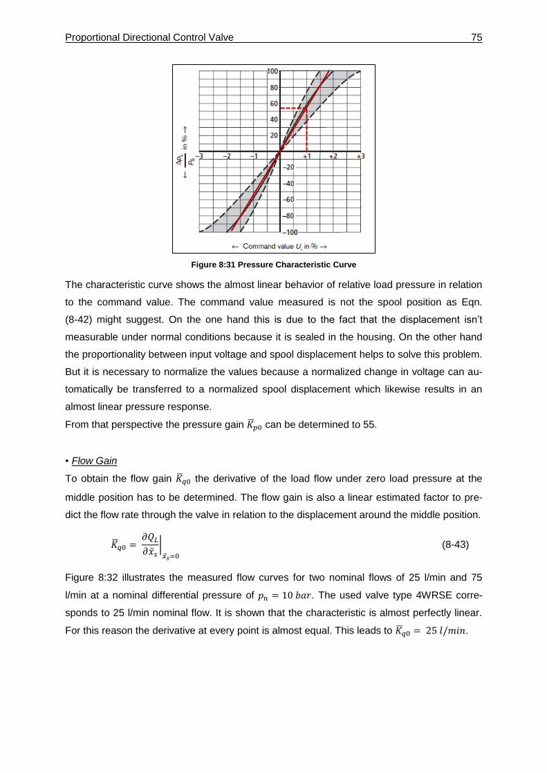
Proportional Directional Control Valve 75
Figure 8:31 Pressure Characteristic Curve
The characteristic curve shows the almost linear behavior of relative load pressure in relation
to the command value. The command value measured is not the spool position as Eqn.
(8-42) might suggest. On the one hand this is due to the fact that the displacement isn’t
measurable under normal conditions because it is sealed in the housing. On the other hand
the proportionality between input voltage and spool displacement helps to solve this problem.
But it is necessary to normalize the values because a normalized change in voltage can au-
tomatically be transferred to a normalized spool displacement which likewise results in an
almost linear pressure response.
From that perspective the pressure gain �̅�𝑝0 can be determined to 55.
▪ Flow Gain
To obtain the flow gain �̅�𝑞0 the derivative of the load flow under zero load pressure at the
middle position has to be determined. The flow gain is also a linear estimated factor to pre-
dict the flow rate through the valve in relation to the displacement around the middle position.
�̅�𝑞0 = 𝜕𝑄𝐿𝜕�̅�𝑠
|�̅�𝑠=0
(8-43)
Figure 8:32 illustrates the measured flow curves for two nominal flows of 25 l/min and 75
l/min at a nominal differential pressure of 𝑝𝑛 = 10 𝑏𝑎𝑟. The used valve type 4WRSE corre-
sponds to 25 l/min nominal flow. It is shown that the characteristic is almost perfectly linear.
For this reason the derivative at every point is almost equal. This leads to �̅�𝑞0 = 25 𝑙/𝑚𝑖𝑛.
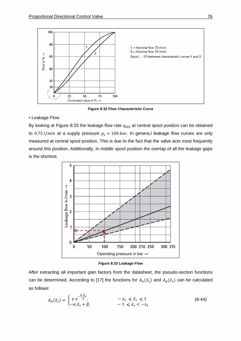
Proportional Directional Control Valve 76
Figure 8:32 Flow Characteristic Curve
▪ Leakage Flow
By looking at Figure 8:33 the leakage flow rate 𝑞𝑙𝑘0 at central spool position can be obtained
to 0.75 𝑙/𝑚𝑖𝑛 at a supply pressure 𝑝𝑠 = 100 𝑏𝑎𝑟. In genera,l leakage flow curves are only
measured at central spool position. This is due to the fact that the valve acts most frequently
around this position. Additionally, in middle spool position the overlap of all the leakage gaps
is the shortest.
Figure 8:33 Leakage Flow
After extracting all important gain factors from the datasheet, the pseudo-section functions
can be determined. According to [17] the functions for 𝐴𝑛(�̅�𝑠) and 𝐴𝑝(�̅�𝑠) can be calculated
as follows:
𝐴𝑛(�̅�𝑠) = {𝛾 𝑒−
𝑘 �̅�𝑠2 , − 𝑥𝑡 ⩽ �̅�𝑠 ⩽ 1
−α �̅�𝑠 + 𝛽, − 1 ⩽ �̅�𝑠 < −𝑥𝑡 (8-44)
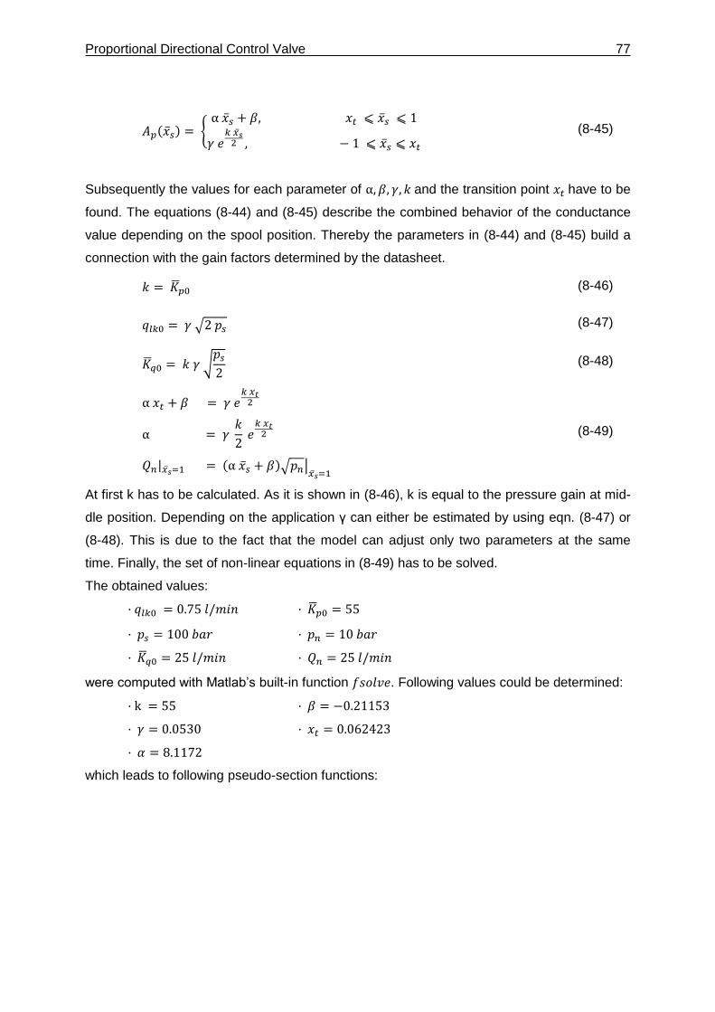
Proportional Directional Control Valve 77
𝐴𝑝(�̅�𝑠) = {α �̅�𝑠 + 𝛽, 𝑥𝑡 ⩽ �̅�𝑠 ⩽ 1
𝛾 𝑒𝑘 �̅�𝑠2 , − 1 ⩽ �̅�𝑠 ⩽ 𝑥𝑡
(8-45)
Subsequently the values for each parameter of α, 𝛽, 𝛾, 𝑘 and the transition point 𝑥𝑡 have to be
found. The equations (8-44) and (8-45) describe the combined behavior of the conductance
value depending on the spool position. Thereby the parameters in (8-44) and (8-45) build a
connection with the gain factors determined by the datasheet.
𝑘 = �̅�𝑝0 (8-46)
𝑞𝑙𝑘0 = 𝛾 √2 𝑝𝑠 (8-47)
�̅�𝑞0 = 𝑘 𝛾 √𝑝𝑠2
(8-48)
α 𝑥𝑡 + 𝛽 = 𝛾 𝑒𝑘 𝑥𝑡2
α = 𝛾 𝑘
2 𝑒𝑘 𝑥𝑡2
𝑄𝑛|�̅�𝑠=1 = (α �̅�𝑠 + 𝛽)√𝑝𝑛|�̅�𝑠=1
(8-49)
At first k has to be calculated. As it is shown in (8-46), k is equal to the pressure gain at mid-
dle position. Depending on the application γ can either be estimated by using eqn. (8-47) or
(8-48). This is due to the fact that the model can adjust only two parameters at the same
time. Finally, the set of non-linear equations in (8-49) has to be solved.
The obtained values:
· 𝑞𝑙𝑘0 = 0.75 𝑙/𝑚𝑖𝑛 · �̅�𝑝0 = 55
· 𝑝𝑠 = 100 𝑏𝑎𝑟 · 𝑝𝑛 = 10 𝑏𝑎𝑟
· �̅�𝑞0 = 25 𝑙/𝑚𝑖𝑛 · 𝑄𝑛 = 25 𝑙/𝑚𝑖𝑛
were computed with Matlab’s built-in function 𝑓𝑠𝑜𝑙𝑣𝑒. Following values could be determined:
· k = 55 · 𝛽 = −0.21153
· 𝛾 = 0.0530 · 𝑥𝑡 = 0.062423
· 𝛼 = 8.1172
which leads to following pseudo-section functions:
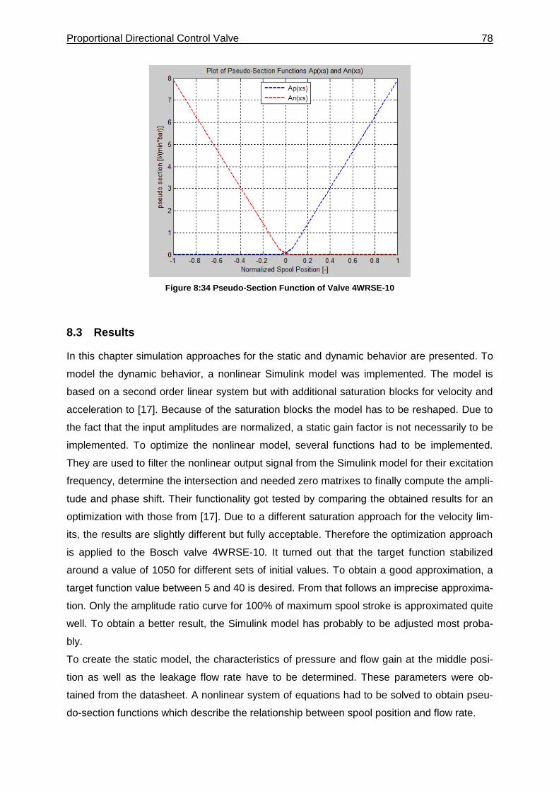
Proportional Directional Control Valve 78
Figure 8:34 Pseudo-Section Function of Valve 4WRSE-10
8.3 Results
In this chapter simulation approaches for the static and dynamic behavior are presented. To
model the dynamic behavior, a nonlinear Simulink model was implemented. The model is
based on a second order linear system but with additional saturation blocks for velocity and
acceleration to [17]. Because of the saturation blocks the model has to be reshaped. Due to
the fact that the input amplitudes are normalized, a static gain factor is not necessarily to be
implemented. To optimize the nonlinear model, several functions had to be implemented.
They are used to filter the nonlinear output signal from the Simulink model for their excitation
frequency, determine the intersection and needed zero matrixes to finally compute the ampli-
tude and phase shift. Their functionality got tested by comparing the obtained results for an
optimization with those from [17]. Due to a different saturation approach for the velocity lim-
its, the results are slightly different but fully acceptable. Therefore the optimization approach
is applied to the Bosch valve 4WRSE-10. It turned out that the target function stabilized
around a value of 1050 for different sets of initial values. To obtain a good approximation, a
target function value between 5 and 40 is desired. From that follows an imprecise approxima-
tion. Only the amplitude ratio curve for 100% of maximum spool stroke is approximated quite
well. To obtain a better result, the Simulink model has probably to be adjusted most proba-
bly.
To create the static model, the characteristics of pressure and flow gain at the middle posi-
tion as well as the leakage flow rate have to be determined. These parameters were ob-
tained from the datasheet. A nonlinear system of equations had to be solved to obtain pseu-
do-section functions which describe the relationship between spool position and flow rate.
79
9 Summary and Discussion
Modelling a hydraulic system, several fundamental observations have to be made. It was
shown which input and output parameters or energy storages are usual in hydraulic systems.
This information is needful to determine balance equations as well as static relations to finally
create a block diagram. On the one hand a block diagram helps to visualize all important
factors which influence the simulated system. On the other hand it is helpful to build up a
model in Simulink.
The proportional directional valve is the most important component in the circuit because of
its controlling performance. Due to that its functionality was described, especially the LVDT.
It was shown how the LVDT translates the input voltage into a linear spool displacement
which is the main requirement for its good controlling abilities. It was pointed out that the
proportional valve can be simplified to a second order spring-mass-damper system. For that
reason, the dynamic behavior of forced oscillations was explained on a linear spring-mass-
damper system in order to understand the dynamic behavior in a better way. It was explained
that in the beginning of the oscillation the excitation frequency superposes with the natural
frequency of the system. Furthermore it was shown that the natural frequency dies out over
time due to the transient effect. Also the impact of a post and subcritical excitation on the
oscillation characteristics was discussed. These considerations are needful to evaluate the
present waveform in a time domain simulation. But usually, hydraulic valve manufacturer use
frequency response curves to illustrate the dynamical behavior of their valves. To be able to
understand these characteristics, frequency response plots were explained precisely. Due to
the fact that the simulation is done in time domain, the connection between time and fre-
quency domain was explained by introducing Fourier transform.
After fundamental considerations, the functionality of all circuit components together as a
system in a closed loop circuit was explained. It is necessary to understand how the system
works and where cutting points exist between the several parts. That helps dividing the main
system into subsystems which simplifies the process of building models and simulating them
due to the lower complexity.
Before subsystems can be created, an oil model needed to be developed. It was assumed
that HLP 46 is used in the circuit. The viscosity, density and compressibility are the key
properties of the oil. They depend from temperature and pressure. Due to the fact that the
positioning unit only operates in short periods of time, the temperature influence was ne-
glected. The density and kinematic viscosity were assumed to be constant. But for the bulk
modulus a model is used which takes into account the dependence on pressure. That means
a higher pressure in a certain capacity causes a higher bulk modulus.
Summary and Discussion 80
After that, the pipe system was the first subsystem which was created. The pipes connect all
the components with each other and they additionally act as pressure energy storage due to
their capacity. From the dimensions and the bulk modulus model, the capacity can be deter-
mined. To simulate the march of pressure, a model of a pump producing a flow rate into a
pipe system without an outlet was created. The simulation result showed a quick and linear
increase of pressure in the pipe system. That increase was faster with a higher pump flow
rate and a lower pipe capacity.
In the next step the hydraulic cylinder was modelled. Due to the fact that there was no
datasheet with specific dimensions available, only a general model could be created. Firstly,
a simplified in- and output flow rate model was created. Using this model, all energy storages
and balance equations could be determined. Additionally, the dynamic balance of forces had
to be incorporated. Thereby the friction force plays an important role. To characterize it
properly, the approach in [13] was used. Among others this approach considers static and
dynamic friction coefficients as well as a decay constant. The friction coefficients were ex-
tracted from [15] whereas it was necessary to make an assumption for the decay constant.
Based on the model, a simulation of the extending piston was made. It could be shown that
the piston extracts with constant velocity and when the end position is reached, it remains
there.
Then, the PRV was modelled based on the dimensions from the manufacturer’s datasheet.
But not all dimensions or material constants which were necessary for the simulation are
pointed out in the datasheet. For this reason the spool dimensions had to be estimated by
the dimensions from the valve housing and the cartridge. Expecting an opening pressure of
200 bar, the spring constant was set to 100000 N/m which led to a preload displacement of
10.1 mm. Based on those assumptions, a model was created in Simulink. The behavior of
the PRV for different pump flow rates in a closed pipe system was examined. It came out that
the valve stabilized quicker the higher the pump flow rate was. But a higher pump flow rate
also caused a higher pressure peak due to the inertia of the system. It can be concluded that
the selected spring constant is well suited for the performance at high pressures. Due to the
fact that the dynamic simulation is mostly based on assumptions, a static model was devel-
oped. Using a PT1 characteristic with a low time constant, the static relationship between
flow rate and pressure could be simulated very well.
Finally, the proportional directional valve was modelled. Due to the non-linear characteristics,
the approach had to be split up into a static and a dynamic valve model. To simulate the non-
linear dynamic behavior, a second order model with velocity and acceleration saturation was
used. All parameters contained in the Simulink model were variable to be able to manipulate
them with Matlab’s optimization function fminsearch. Doing so, the optimization function tries
to find the best possible model parameters to minimize the error between the measured data
Summary and Discussion 81
points given from the frequency response curves and the Simulink model. For that to realize,
the non-linear model had to be simulated for several excitation frequencies. Thereby the sat-
uration blocks cause harmonics. For that reason a filter function was developed in Matlab to
exclude those. Furthermore, functions for finding intersections, determining zero-matrixes
and computing the amplitude and phase shift were developed as well to create simulated
frequency response curves in order to compare simulation with reality. A proper functionality
of those functions was shown for an optimization of a linear second order Simulink model.
Also the optimization for the non-linear hydraulic valve KBSDG4V-3 led to good results when
compared to [17]. Nevertheless, the optimization for the Bosch valve 4WRSE-10 showed big
deviations for the amplitude response of 10% and 25% of maximum spool stroke. This is
reasoned by the Simulink model which has to be adjusted more properly to the frequency
response curves of the 4WRSE-10 valve.
For the static model, pressure, flow and leakage gain as well as supply and nominal pressure
had to be determined from the valve’s datasheet. Thus it was possible to solve several non-
linear equations for values which describe the behavior of positive and negative pseudo-
section functions. These functions can be understood as conductance values which gives
information about the flow rate through the valve at a certain normalized spool position. It has
shown how the gain parameters can be obtained from the datasheet and how the final char-
acteristics look like.
The methodologies and developed models were subsequently tested with manufacturer’s
data. The good quality of results seems to support the adopted approach.
82
10 Recommendations for Future Work
To pursue this work in the future, several tasks have to be complied. As it is mentioned in the
previous chapter, the hydraulic cylinder’s friction force model is based on assumptions which
needed to be made. With this data the friction force model has to be adapted better on the
real behavior. It can be achieved by changing the certain parameters such as decay constant
𝑇𝑉. It is necessary to mention that extending and retracting characteristic is not equal most
likely.
As long as there is no measurement data available for the PRV, static characteristic shall be
used.
The Simulink model for obtaining the dynamic behavior of the proportional directional valve
needs to be adapted better to the curves in the datasheet. Therefore [17] provides ap-
proaches which can be useful for further considerations. Also the time constant needs to be
optimized to determine the phase shift. Finally, the different models have to be connected to
each other.
It will be also important in the future to validate the model the built model by comparison with
a real hydraulic circuit.
83
11 Reference List
[1] J. Lunze, Regelungstechnik 1: Systemtheoretische Grundlagen, Analyse und Entwurf
einschleifiger Regelungen, Springer, 2008.
[2] W. Dieter and G. Norbert, Hydraulik - Grundlagen, Komponenten, Systeme, vol. 6,
Berlin-Heidelberg: Springer Verlag, 2015.
[3] H. Watter, Hydraulik und Pneumatik, Grundlagen und Übungen - Anwendungen und
Simulation, vol. 4, Wiesbaden: Springer Vieweg, 2015.
[4] D. Will, H. Ströhl und N. Gebhardt, Hydraulik - Grundlagen, Komponenten,
Schaltungen, Berlin: Springer, 1999.
[5] "Bosch Rexroth Web Page," Bosch Rexroth, [Online]. Available: https://dc-
us.resource.bosch.com/media/us/products_13/product_groups_1/industrial_hydraulics
_5/pdfs_4/re29067.pdf. [Accessed 15 July 2016].
[6] "National Instruments Web Page," National Instruments, [Online]. Available:
http://www.ni.com/white-paper/3638/en/. [Accessed 10 July 2016].
[7] J. Dankert und H. Dankert, Technische Mechanik, Wiesbaden: Vieweg+Teubner,
2009.
[8] "University of Koblenz," [Online]. Available: https://www.uni-
koblenz.de/~physik/informatik/DSV/Faltung.pdf. [Accessed 28 06 2016].
[9] "Stack Exchange," [Online]. Available: http://i.stack.imgur.com/Ofkna.png. [Accessed
23 06 2016].
[10] M. Werner, Digitale Signalverarbeitung mit Matlab, 4. ed., Wiesbaden:
Vieweg+Teubner, 2009.
[11] "Cartechnik Hydrauliköle," ATR, [Online]. Available:
http://www.atr.de/fileadmin/downloads/Cartechnic/Produktinfos/LM_PB_Hydraulikoel_
HLP_46.pdf. [Accessed 02 07 2016].
[12] T. Pinheiro, "Conceção e pré-dimensionamento de um sistema de frenagem para um
Tuned Mass Damper," Porto, 2014.
[13] P. Beater, Entwurf hydraulischer Maschinen, Berlin Heidelberg: Springer, 1999.
[14] "Homepage Bosch Rexroth," [Online]. Available:
https://www.boschrexroth.com/various/utilities/mediadirectory/index.jsp?publication=N
ET&ccat_id=20000&remindCcat=on&pagesize=50&search_action=submit&language=
de&search_query=25402&MEDIA_TYPE=Datenblatt&History=p545161&DisplayType=
Reference List 84
pict. [Accessed 15 July 2016].
[15] "Coefficient Summary," [Online]. Available: http://www.schweizer-
fn.de/stoff/reibwerte/reibwerte.php. [Accessed 28 07 2016].
[16] B. Bestmann, "Entwicklung eines Simulationsmodells für eine hydraulische
Positioniervorrichtung," Hamburg University of Applied Sciences, 2005.
[17] J. A. Ferreira, F. Gomes de Almeida and M. R. Quintas, "Semi-empirical model for a
hydraulic servo-solenoid valve," IMechE, 2002.
[18] "Mathworks," [Online]. Available:
http://www.mathworks.com/help/matlab/ref/fminsearch.html. [Accessed 03 08 2016].
[19] J. A. F. Ferreira, "Modelacao de Sistemas Hydraulicos para Simulacao com HArdware-
in-the-Loop," 2002.
[20] "MIT Official Home Page," [Online]. Available: http://ocw.mit.edu/courses/mechanical-
engineering/2-003-modeling-dynamics-and-control-i-spring-2005/labs/lab3fig3.gif.
[Accessed 20 June 2016].
[21] N. Hanson. [Online]. Available:
http://www.cmafh.com/enewsletter/PDFs/Hydraulic_Proportional_Closed_Loop_Syste
m_Design.pdf. [Accessed 10 July 2016].
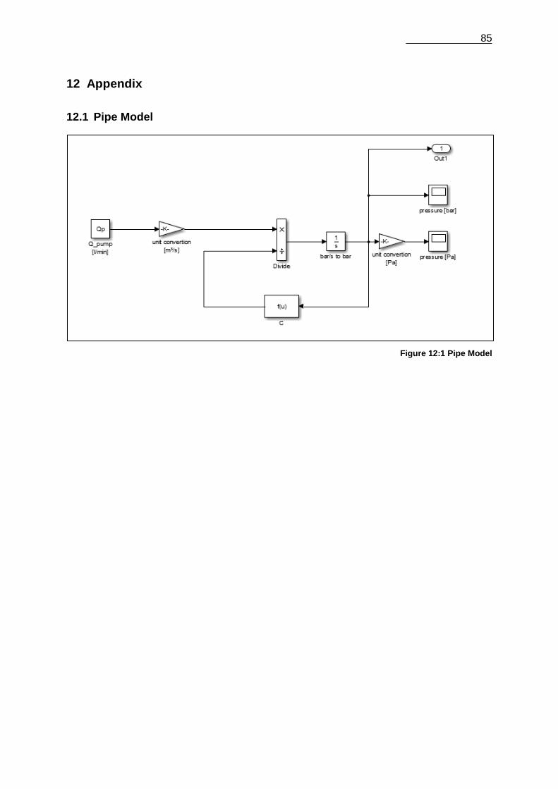
85
12 Appendix
12.1 Pipe Model
Figure 12:1 Pipe Model
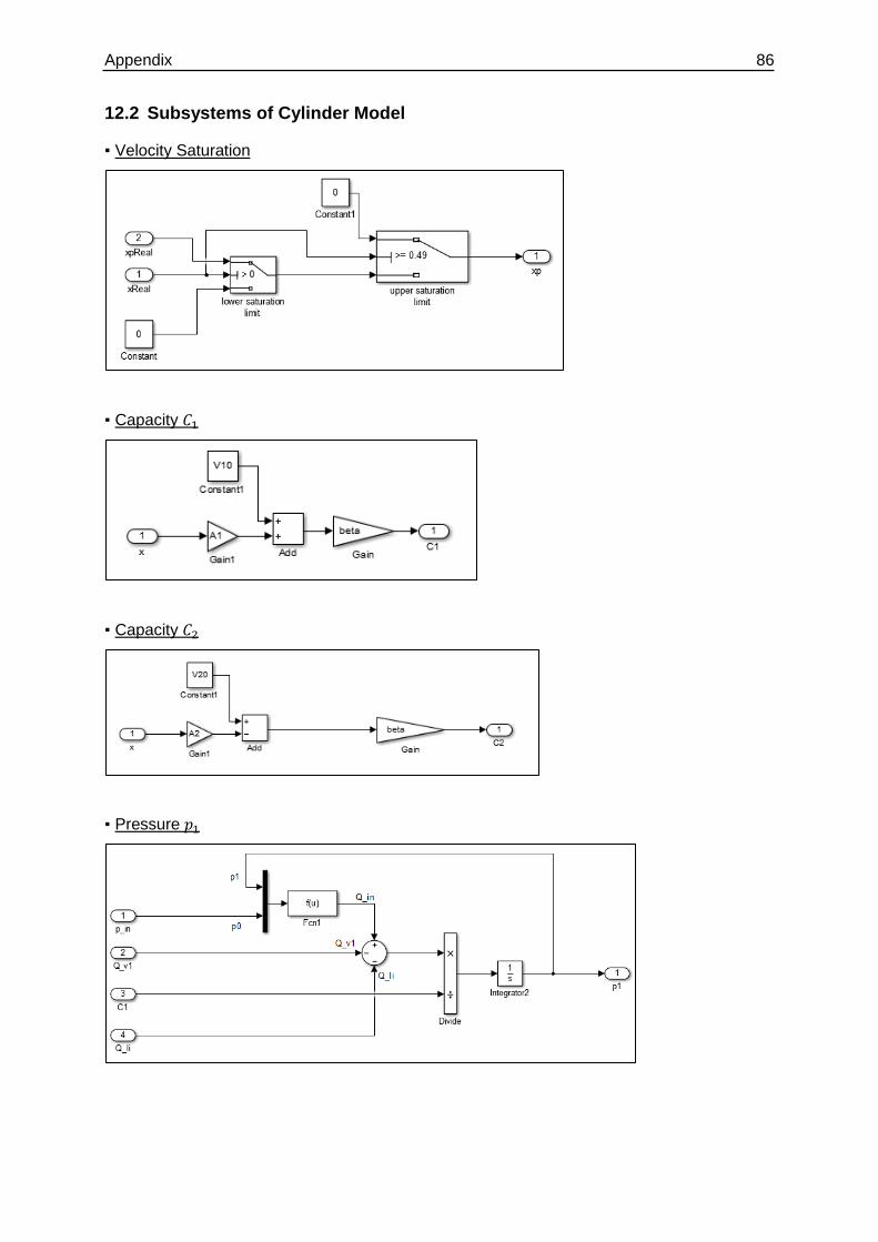
Appendix 86
12.2 Subsystems of Cylinder Model
▪ Velocity Saturation
▪ Capacity 𝐶1
▪ Capacity 𝐶2
▪ Pressure 𝑝1
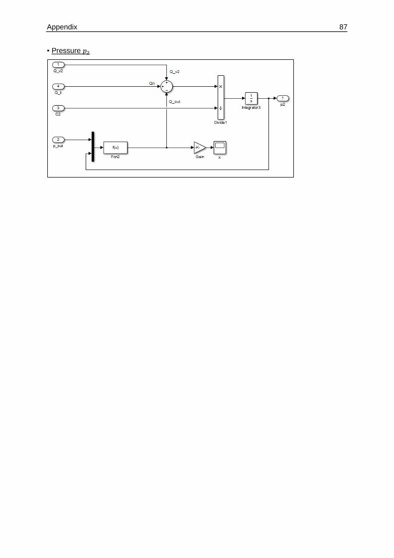
Appendix 87
▪ Pressure 𝑝2
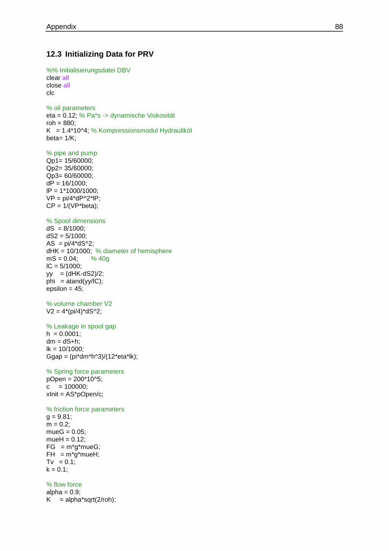
Appendix 88
12.3 Initializing Data for PRV
%% Initialisierungsdatei DBV clear all close all clc % oil parameters eta = 0.12; % Pa*s -> dynamische Viskosität roh = 880; K = 1.4*10^4; % Kompressionsmodul Hydrauliköl beta= 1/K; % pipe and pump Qp1= 15/60000; Qp2= 35/60000; Qp3= 60/60000; dP = 16/1000; lP = 1*1000/1000; VP = pi/4*dP^2*lP; CP = 1/(VP*beta); % Spool dimensions dS = 8/1000; dS2 = 5/1000; AS = pi/4*dS^2; dHK = 10/1000; % diameter of hemisphere mS = 0.04; % 40g lC = 5/1000; yy = (dHK-dS2)/2; phi = atand(yy/lC); epsilon = 45; % volume chamber V2 V2 = 4*(pi/4)*dS^2; % Leakage in spool gap h = 0.0001; dm = dS+h; lk = 10/1000; Ggap = (pi*dm*h^3)/(12*eta*lk); % Spring force parameters pOpen = 200*10^5; c = 100000; xInit = AS*pOpen/c; % friction force parameters g = 9.81; m = 0.2; mueG = 0.05; mueH = 0.12; FG = m*g*mueG; FH = m*g*mueH; Tv = 0.1; k = 0.1; % flow force alpha = 0.9; K = alpha*sqrt(2/roh);
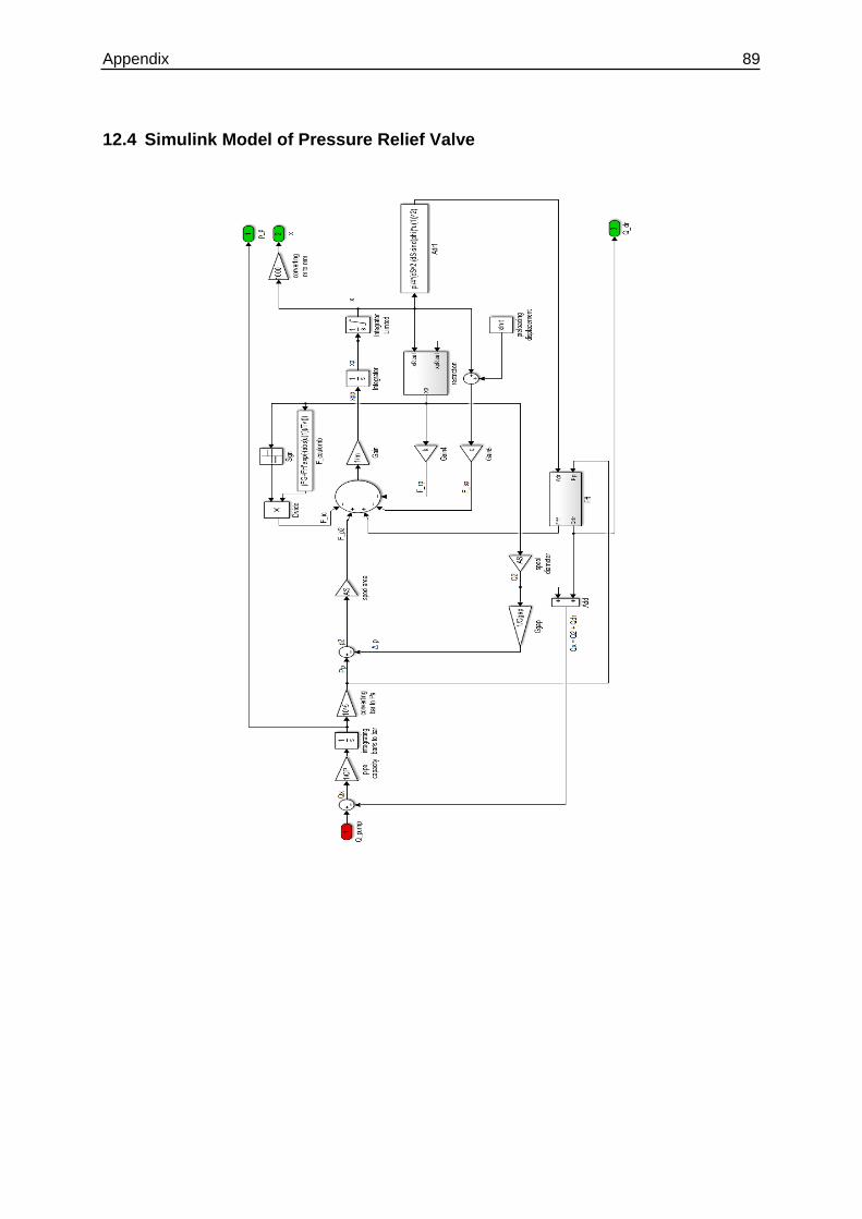
Appendix 89
12.4 Simulink Model of Pressure Relief Valve
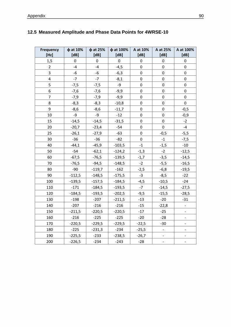
Appendix 90
12.5 Measured Amplitude and Phase Data Points for 4WRSE-10
Frequency [Hz]
φ at 10% [dB]
φ at 25% [dB]
φ at 100% [dB]
A at 10% [dB]
A at 25% [dB]
A at 100% [dB]
1,5 0 0 0 0 0 0
2 -4 -4 -4,5 0 0 0
3 -6 -6 -6,3 0 0 0
4 -7 -7 -8,1 0 0 0
5 -7,5 -7,5 -9 0 0 0
6 -7,6 -7,6 -9,9 0 0 0
7 -7,9 -7,9 -9,9 0 0 0
8 -8,3 -8,3 -10,8 0 0 0
9 -8,6 -8,6 -11,7 0 0 -0,5
10 -9 -9 -12 0 0 -0,9
15 -14,5 -14,5 -31,5 0 0 -2
20 -20,7 -23,4 -54 0 0 -4
25 -26,1 -27,9 -63 0 -0,5 -5,5
30 -36 -36 -82 0 -1 -7,5
40 -44,1 -45,9 -103,5 -1 -1,5 -10
50 -54 -62,1 -124,2 -1,3 -2 -12,5
60 -67,5 -76,5 -139,5 -1,7 -3,5 -14,5
70 -76,5 -94,5 -148,5 -2 -5,5 -16,5
80 -90 -119,7 -162 -2,5 -6,8 -19,5
90 -112,5 -148,5 -175,5 -3 -8,5 -22
100 -139,5 -157,5 -184,5 -4,5 -10,5 -24
110 -171 -184,5 -193,5 -7 -14,5 -27,5
120 -184,5 -193,5 -202,5 -9,5 -15,5 -28,5
130 -198 -207 -211,5 -13 -20 -31
140 -207 -216 -216 -15 -22,8 -
150 -211,5 -220,5 -220,5 -17 -25 -
160 -216 -225 -225 -20 -28 -
170 -220,5 -229,5 -229,5 -22,5 -30 -
180 -225 -231,3 -234 -25,5 - -
190 -225,5 -233 -238,5 -26,7 - -
200 -226,5 -234 -243 -28 - -
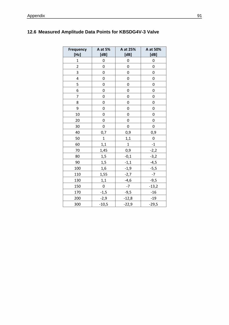
Appendix 91
12.6 Measured Amplitude Data Points for KBSDG4V-3 Valve
Frequency [Hz]
A at 5% [dB]
A at 25% [dB]
A at 50% [dB]
1 0 0 0
2 0 0 0
3 0 0 0
4 0 0 0
5 0 0 0
6 0 0 0
7 0 0 0
8 0 0 0
9 0 0 0
10 0 0 0
20 0 0 0
30 0 0 0
40 0,7 0,9 0,9
50 1 1,1 0
60 1,1 1 -1
70 1,45 0,9 -2,2
80 1,5 -0,1 -3,2
90 1,5 -1,1 -4,5
100 1,6 -1,9 -5,5
110 1,55 -2,7 -7
130 1,1 -4,6 -9,5
150 0 -7 -13,2
170 -1,5 -9,5 -16
200 -2,9 -12,8 -19
300 -10,5 -22,9 -29,5
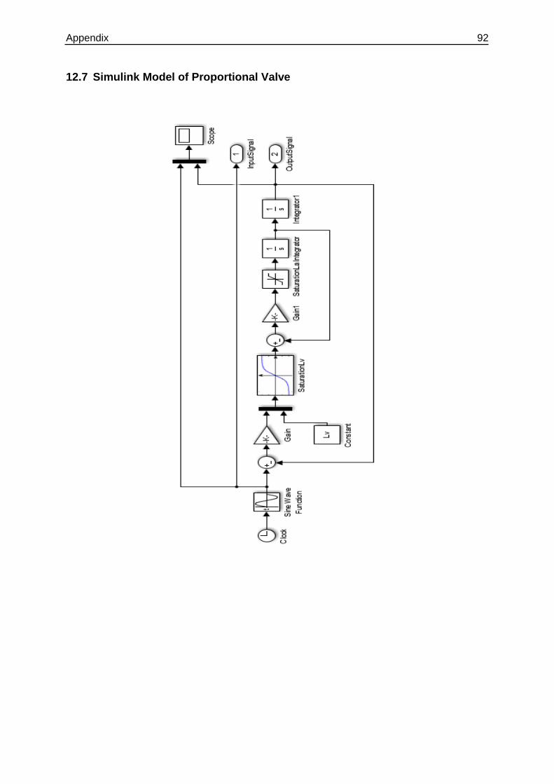
Appendix 92
12.7 Simulink Model of Proportional Valve