Simulating Quadrotor UAVs in Outdoor ScenariosAndrew Symington, Renzo De Nardi, Simon Julier and Stephen Hailes

{a.symington,r.denardi,s.julier,s.hailes}@ucl.ac.uk

Abstract—Motivated by the risks and costs associated withoutdoor experiments, this paper presents a new multi-platformquadrotor simulator. The simulator implements a novel second-order dynamic model for a quadrotor, produced through evo-lutionary programming, and explained by domain knowledge.The model captures the effects of mechanics, aerodynamics,wind and rotational stabilization control on the flight platform.In addition, the simulator implements military-grade modelsfor wind and turbulence, as well as noise models for satellitenavigation, barometric altitude and orientation. The usefulnessof the simulator is shown qualitatively by a comparing howcoloured and white position noise affect the performance ofoffline, range-only SLAM. The simulator is intended to beused for planning experiments, or for stress-testing applicationperformance over a wide range of operating conditions.

Index Terms—Unmanned Aerial Systems, Simulation

I. INTRODUCTION

Unmanned aerial vehicles (UAVs) have received significant

research attention as a result of the numerous military and

civilian applications that they enable. Quadrotors have proven

themselves as favourable platforms for research, since they

are inexpensive, easy to fly, agile and safe to operate [1].

Conducting outdoor experiments with quadrotors requires

ideal weather conditions and compliance with local aviation

regulations, uses significant resources, and puts platforms at

risk. It is therefore preferable to evaluate scenarios in sim-

ulation prior to experimentation, where possible. However,

the suitability of such an approach depends largely on the

fidelity of the simulator. The work in this paper is therefore

motivated by the need for a quadrotor simulator that (i)

enables multiple platforms to be simulated at the application

level, (ii) provides realistic models for dynamics, wind and

sensor noise, and (iii) balances accuracy with speed, thereby

enabling real-time, or near real-time, performance.

A great number of simulators exist as tools to for training

radio control enthusiasts, but not as platforms for research.

Research simulators based on first principles have been devel-

oped for USARSim [2] and Gazebo [3]. Both capture the be-

haviour of an ideal platform’s mechanics and aerodynamics,

but not of the low-level controller used to perform rotational

stabilization control. The design of the stabilization control

algorithm is usually proprietary, and therefore cannot be

modelled by first principles. Although effort has been made

to investigate the effect of wind and turbulence on quadrotor

dynamics [4], such research remains to be integrated into the

widely-used simulators. More recent simulators are based on

the Robotic Operating System (ROS) and include SwarmSim

X [5] and Hector Quadrotor [6], which use a PhysX and

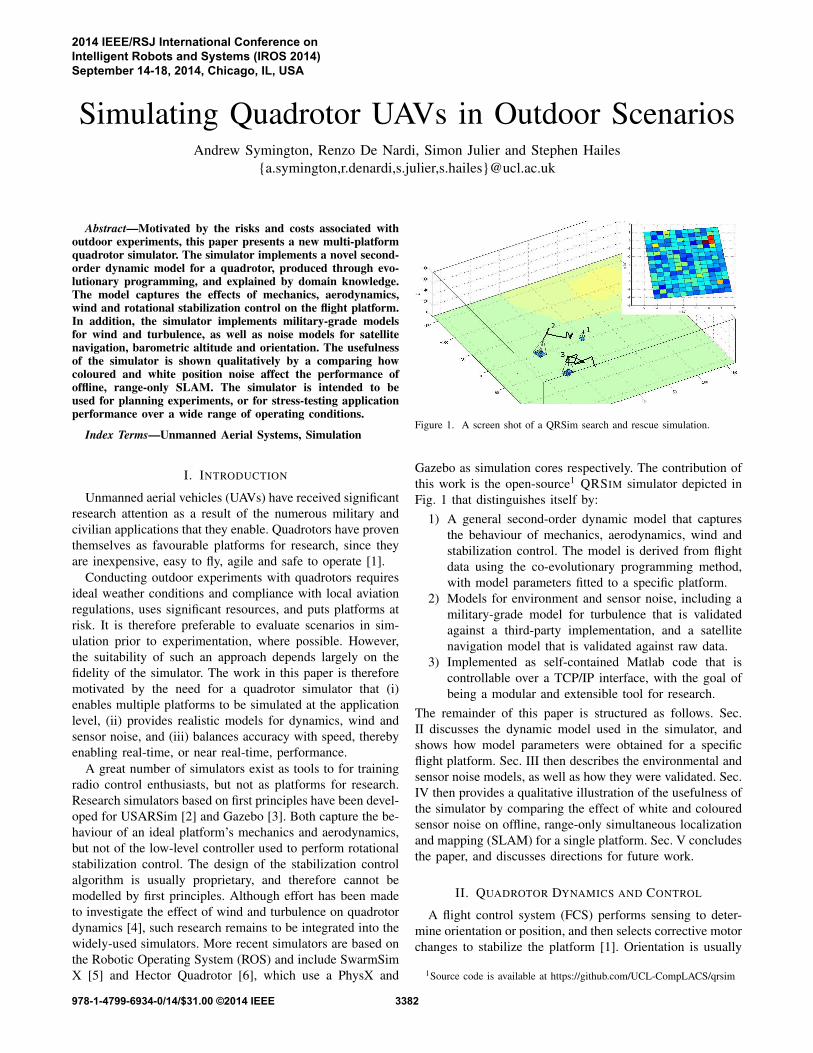
Figure 1. A screen shot of a QRSim search and rescue simulation.

Gazebo as simulation cores respectively. The contribution of

this work is the open-source1 QRSIM simulator depicted in

Fig. 1 that distinguishes itself by:

1) A general second-order dynamic model that captures

the behaviour of mechanics, aerodynamics, wind and

stabilization control. The model is derived from flight

data using the co-evolutionary programming method,

with model parameters fitted to a specific platform.

2) Models for environment and sensor noise, including a

military-grade model for turbulence that is validated

against a third-party implementation, and a satellite

navigation model that is validated against raw data.

3) Implemented as self-contained Matlab code that is

controllable over a TCP/IP interface, with the goal of

being a modular and extensible tool for research.

The remainder of this paper is structured as follows. Sec.

II discusses the dynamic model used in the simulator, and

shows how model parameters were obtained for a specific

flight platform. Sec. III then describes the environmental and

sensor noise models, as well as how they were validated. Sec.

IV then provides a qualitative illustration of the usefulness of

the simulator by comparing the effect of white and coloured

sensor noise on offline, range-only simultaneous localization

and mapping (SLAM) for a single platform. Sec. V concludes

the paper, and discusses directions for future work.

II. QUADROTOR DYNAMICS AND CONTROL

A flight control system (FCS) performs sensing to deter-

mine orientation or position, and then selects corrective motor

changes to stabilize the platform [1]. Orientation is usually

1Source code is available at https://github.com/UCL-CompLACS/qrsim

2014 IEEE/RSJ International Conference onIntelligent Robots and Systems (IROS 2014)September 14-18, 2014, Chicago, IL, USA

978-1-4799-6934-0/14/$31.00 ©2014 IEEE 3382

3383

Z,W, r, 4J

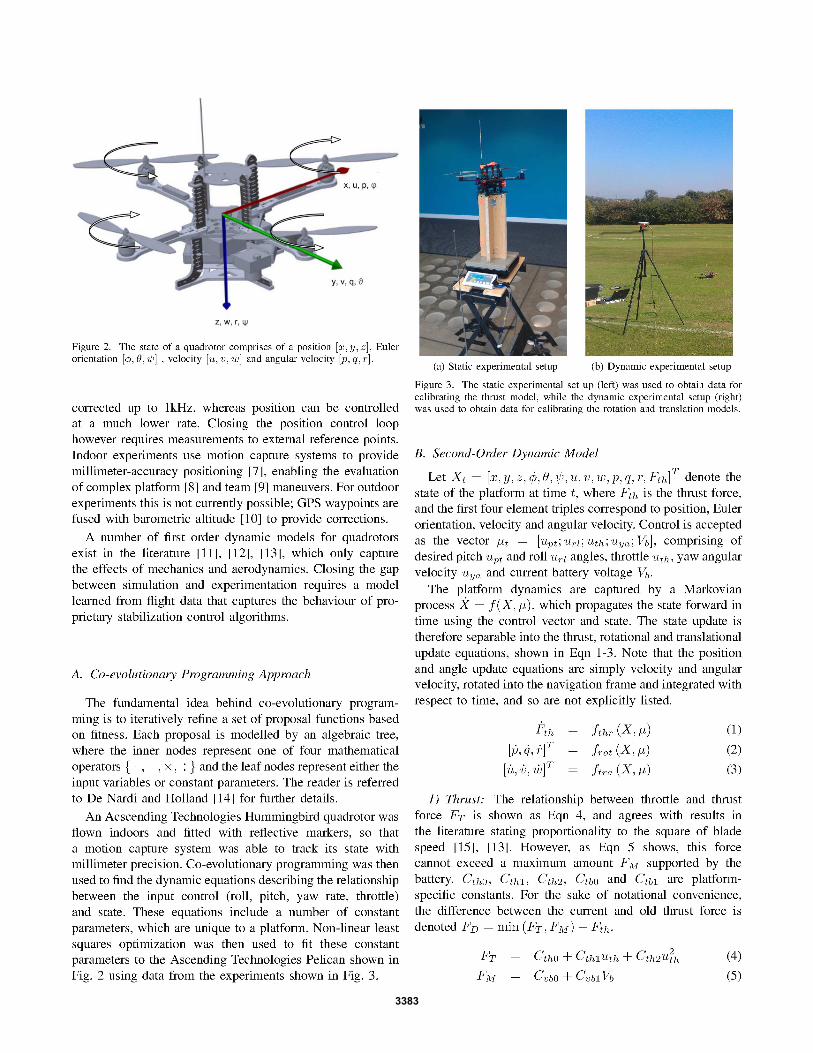
Figure 2. The state of a quadrotor comprises of a position [x, y, z], Eulerorientation [c/J, B, 7jJ] , velocity [u,v, w] and angular velocity [p, q,r].

(a) Static experimental setup (b) Dynamic experimental setup

Figure 3. The static experimental set up (left) was used to obtain data forcalibrating the thrust model, while the dynamic experimental setup (right)was used to obtain data for calibrating the rotation and translation models.

1) Thrust: The relationship between throttle and thrustforce FT is shown as Eqn 4, and agrees with results inthe literature stating proportionality to the square of bladespeed [15], [13]. However, as Eqn 5 shows, this forcecannot exceed a maximum amount FM supported by thebattery. CthO, Cth1, Cth2, CtbO and Ctb1 are platform­specific constants. For the sake of notational convenience,the difference between the current and old thrust force isdenoted F D = min (FT, F M) - Fth.

B. Second-Order Dynamic Model

Let X, = [x,y,z,¢,B,'if;,u,v,w,p,q,r,Fth]T denote thestate of the platform at time t, where F th is the thrust force,and the first four element triples correspond to position, Eulerorientation, velocity and angular velocity. Control is acceptedas the vector Ilt = [Upt; Uri; Uth; Uya; Vb], comprising ofdesired pitch Upt and roll Uri angles, throttle Uth, yaw angularvelocity u ya and current battery voltage Vb.

The platform dynamics are captured by a Markovianprocess X = f(X, Il), which propagates the state forward intime using the control vector and state. The state update istherefore separable into the thrust, rotational and translationalupdate equations, shown in Eqn 1-3. Note that the positionand angle update equations are simply velocity and angularvelocity, rotated into the navigation frame and integrated withrespect to time, and so are not explicitly listed.

CthO+ Cth1Uth + Cth2UZh

c.: + CVb1Vb

(4)

(5)

(1)

(2)

(3)

fthr (X, Il)

frat (X, Il)

ftra (X, Il)

Fth

[p,q,r]T[ ' , ']Tu,v,w

The fundamental idea behind co-evolutionary program­ming is to iteratively refine a set of proposal functions basedon fitness. Each proposal is modelled by an algebraic tree,where the inner nodes represent one of four mathematicaloperators {+, -, x ,~} and the leaf nodes represent either theinput variables or constant parameters. The reader is referredto De Nardi and Holland [14] for further details.

An Acscending Technologies Hummingbird quadrotor wasflown indoors and fitted with reflective markers, so thata motion capture system was able to track its state withmillimeter precision. Co-evolutionary programming was thenused to find the dynamic equations describing the relationshipbetween the input control (roll, pitch, yaw rate, throttle)and state. These equations include a number of constantparameters, which are unique to a platform. Non-linear leastsquares optimization was then used to fit these constantparameters to the Ascending Technologies Pelican shown inFig. 2 using data from the experiments shown in Fig. 3.

corrected up to 1kHz, whereas positron can be controlledat a much lower rate. Closing the position control loophowever requires measurements to external reference points.Indoor experiments use motion capture systems to providemillimeter-accuracy positioning [7], enabling the evaluationof complex platform [8] and team [9] maneuvers. For outdoorexperiments this is not currently possible; GPS waypoints arefused with barometric altitude [10] to provide corrections.

A number of first order dynamic models for quadrotorsexist in the literature [11], [12], [13], which only capturethe effects of mechanics and aerodynamics. Closing the gapbetween simulation and experimentation requires a modellearned from flight data that captures the behaviour of pro­prietary stabilization control algorithms.

A. Co-evolutionary Programming Approach

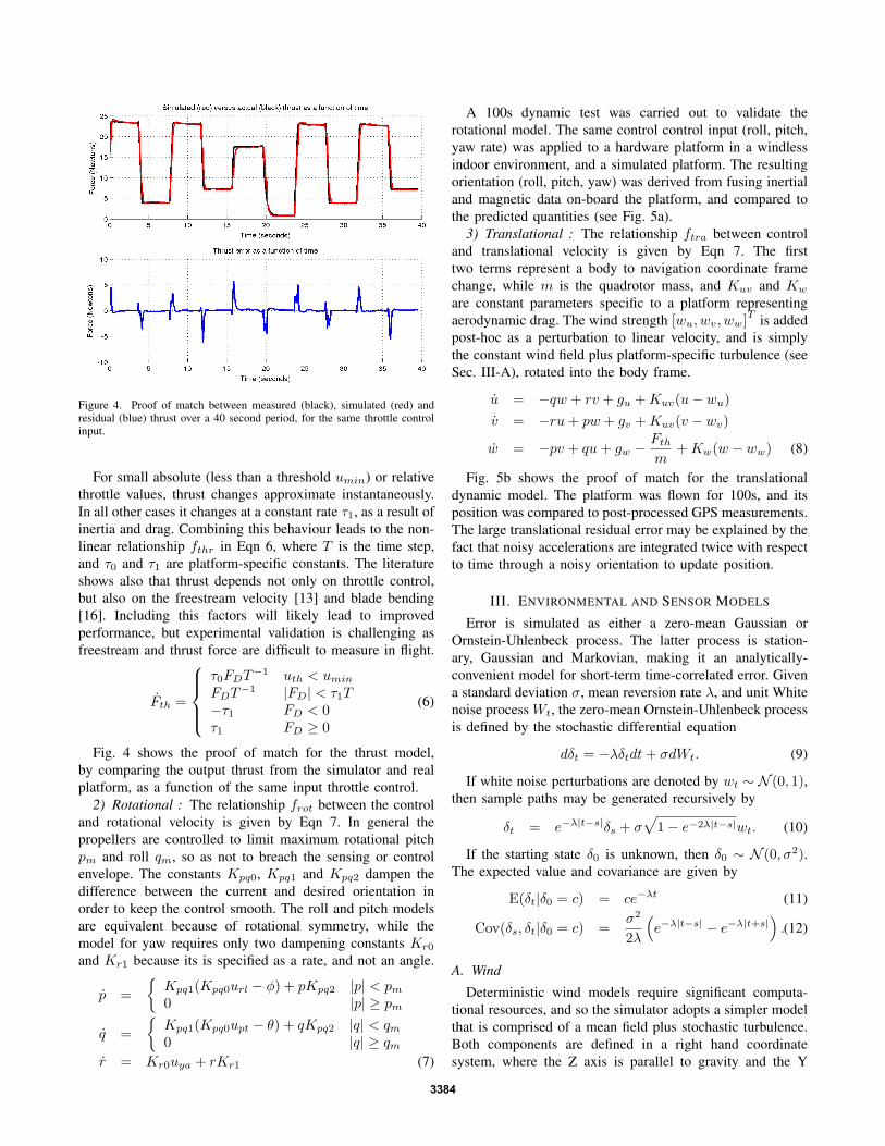
Figure 4. Proof of match between measured (black), simulated (red) andresidual (blue) thrust over a 40 second period, for the same throttle controlinput.

For small absolute (less than a threshold umin) or relative

throttle values, thrust changes approximate instantaneously.

In all other cases it changes at a constant rate τ1, as a result of

inertia and drag. Combining this behaviour leads to the non-

linear relationship fthr in Eqn 6, where T is the time step,

and τ0 and τ1 are platform-specific constants. The literature

shows also that thrust depends not only on throttle control,

but also on the freestream velocity [13] and blade bending

[16]. Including this factors will likely lead to improved

performance, but experimental validation is challenging as

freestream and thrust force are difficult to measure in flight.

Fth =

τ0FDT−1 uth < umin

FDT−1 |FD| < τ1T

−τ1 FD < 0τ1 FD ≥ 0

(6)

Fig. 4 shows the proof of match for the thrust model,

by comparing the output thrust from the simulator and real

platform, as a function of the same input throttle control.

2) Rotational : The relationship frot between the control

and rotational velocity is given by Eqn 7. In general the

propellers are controlled to limit maximum rotational pitch

pm and roll qm, so as not to breach the sensing or control

envelope. The constants Kpq0, Kpq1 and Kpq2 dampen the

difference between the current and desired orientation in

order to keep the control smooth. The roll and pitch models

are equivalent because of rotational symmetry, while the

model for yaw requires only two dampening constants Kr0

and Kr1 because its is specified as a rate, and not an angle.

p =

{

Kpq1(Kpq0url − φ) + pKpq2 |p| < pm0 |p| ≥ pm

q =

{

Kpq1(Kpq0upt − θ) + qKpq2 |q| < qm0 |q| ≥ qm

r = Kr0uya + rKr1 (7)

A 100s dynamic test was carried out to validate the

rotational model. The same control control input (roll, pitch,

yaw rate) was applied to a hardware platform in a windless

indoor environment, and a simulated platform. The resulting

orientation (roll, pitch, yaw) was derived from fusing inertial

and magnetic data on-board the platform, and compared to

the predicted quantities (see Fig. 5a).

3) Translational : The relationship ftra between control

and translational velocity is given by Eqn 7. The first

two terms represent a body to navigation coordinate frame

change, while m is the quadrotor mass, and Kuv and Kw

are constant parameters specific to a platform representing

aerodynamic drag. The wind strength [wu, wv, ww]T

is added

post-hoc as a perturbation to linear velocity, and is simply

the constant wind field plus platform-specific turbulence (see

Sec. III-A), rotated into the body frame.

u = −qw + rv + gu +Kuv(u− wu)

v = −ru+ pw + gv +Kuv(v − wv)

w = −pv + qu+ gw −Fth

m+Kw(w − ww) (8)

Fig. 5b shows the proof of match for the translational

dynamic model. The platform was flown for 100s, and its

position was compared to post-processed GPS measurements.

The large translational residual error may be explained by the

fact that noisy accelerations are integrated twice with respect

to time through a noisy orientation to update position.

III. ENVIRONMENTAL AND SENSOR MODELS

Error is simulated as either a zero-mean Gaussian or

Ornstein-Uhlenbeck process. The latter process is station-

ary, Gaussian and Markovian, making it an analytically-

convenient model for short-term time-correlated error. Given

a standard deviation σ, mean reversion rate λ, and unit White

noise process Wt, the zero-mean Ornstein-Uhlenbeck process

is defined by the stochastic differential equation

dδt = −λδtdt+ σdWt. (9)

If white noise perturbations are denoted by wt ∼ N (0, 1),then sample paths may be generated recursively by

δt = e−λ|t−s|δs + σ√

1− e−2λ|t−s|wt. (10)

If the starting state δ0 is unknown, then δ0 ∼ N (0, σ2).The expected value and covariance are given by

E(δt|δ0 = c) = ce−λt (11)

Cov(δs, δt|δ0 = c) =σ2

2λ

(

e−λ|t−s| − e−λ|t+s|)

.(12)

A. Wind

Deterministic wind models require significant computa-

tional resources, and so the simulator adopts a simpler model

that is comprised of a mean field plus stochastic turbulence.

Both components are defined in a right hand coordinate

system, where the Z axis is parallel to gravity and the Y

3384

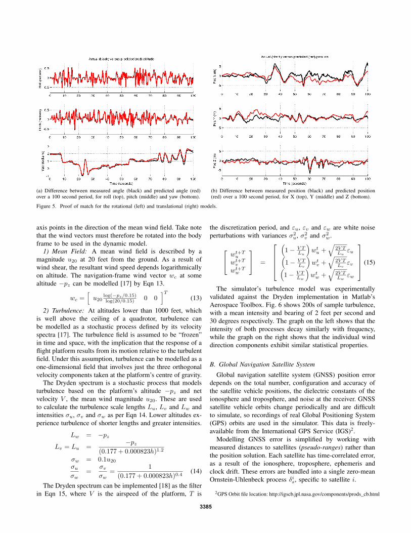
(a) Difference between measured angle (black) and predicted angle (red)over a 100 second period, for roll (top), pitch (middle) and yaw (bottom).

(b) Difference between measured position (black) and predicted position(red) over a 100 second period, for X (top), Y (middle) and Z (bottom).

Figure 5. Proof of match for the rotational (left) and translational (right) models.

axis points in the direction of the mean wind field. Take note

that the wind vectors must therefore be rotated into the body

frame to be used in the dynamic model.

1) Mean Field: A mean wind field is described by a

magnitude u20 at 20 feet from the ground. As a result of

wind shear, the resultant wind speed depends logarithmically

on altitude. The navigation-frame wind vector wc at some

altitude −pz can be modelled [17] by Eqn 13.

wc =[

u20log(−pz/0.15)log(20/0.15) 0 0

]T

(13)

2) Turbulence: At altitudes lower than 1000 feet, which

is well above the ceiling of a quadrotor, turbulence can

be modelled as a stochastic process defined by its velocity

spectra [17]. The turbulence field is assumed to be “frozen”

in time and space, with the implication that the response of a

flight platform results from its motion relative to the turbulent

field. Under this assumption, turbulence can be modelled as a

one-dimensional field that involves just the three orthogonal

velocity components taken at the platform’s centre of gravity.

The Dryden spectrum is a stochastic process that models

turbulence based on the platform’s altitude −pz and net

velocity V , the mean wind magnitude u20. These are used

to calculate the turbulence scale lengths Lu, Lv and Lw and

intensities σu, σv and σw as per Eqn 14. Lower altitudes ex-

perience turbulence of shorter lengths and greater intensities.

Lw = −pz

Lv = Lu =−pz

(0.177 + 0.000823h)1.2

σw = 0.1u20

σu

σw=

σv

σw=

1

(0.177 + 0.000823h)0.4(14)

The Dryden spectrum can be implemented [18] as the filter

in Eqn 15, where V is the airspeed of the platform, T is

the discretization period, and εu, εv and εw are white noise

perturbations with variances σ2u, σ2

v and σ2w.

wt+Tu

wt+Tv

wt+Tw

=

(

1− V TLu

)

wtu +√

2V TLu

εu(

1− V TLv

)

wtv +√

2V TLv

εv(

1− V TLw

)

wtw +√

2V TLw

εw

(15)

The simulator’s turbulence model was experimentally

validated against the Dryden implementation in Matlab’s

Aerospace Toolbox. Fig. 6 shows 200s of sample turbulence,

with a mean intensity and bearing of 2 feet per second and

30 degrees respectively. The graph on the left shows that the

intensity of both processes decay similarly with frequency,

while the graph on the right shows that the individual wind

direction components exhibit similar statistical properties.

B. Global Navigation Satellite System

Global navigation satellite system (GNSS) position error

depends on the total number, configuration and accuracy of

the satellite vehicle positions, the dielectric constants of the

ionosphere and troposphere, and noise at the receiver. GNSS

satellite vehicle orbits change periodically and are difficult

to simulate, so recordings of real Global Positioning System

(GPS) orbits are used in the simulator. This data is freely-

available from the International GPS Service (IGS)2.

Modelling GNSS error is simplified by working with

measured distances to satellites (pseudo-ranges) rather than

the position solution. Each satellite has time-correlated error,

as a result of the ionosphere, troposphere, ephemeris and

clock drift. These errors are bundled into a single zero-mean

Ornstein-Uhlenbeck process δis, specific to satellite i.

2GPS Orbit file location: http://igscb.jpl.nasa.gov/components/prods_cb.html

3385

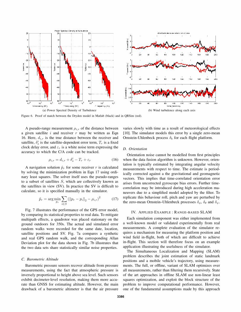
(a) Power Spectral Density of Turbulence (b) Wind turbulence along each axis

Figure 6. Proof of match between the Dryden model in Matlab (black) and in QRSim (red).

A pseudo-range measurement ρi,r of the distance between

a given satellite i and receiver r may be written as Eqn

16. Here, di,r is the true distance between the receiver and

satellite, δis is the satellite-dependent error term, Tr is a fixed

clock delay error, and εr is a white noise term expressing the

accuracy to which the C/A code can be tracked.

ρi,r = di,r + δis − Tr + εr (16)

A navigation solution pr for some receiver r is calculated

by solving the minimization problem in Eqn 17 using ordi-

nary least squares. The solver itself uses the pseudo-ranges

to a subset of satellites S, which are collectively known as

the satellites in view (SV). In practice the SV is difficult to

calculate, so it is specified manually in the simulator.

pr = argminpr

∑

i∈S

(‖pr − pi‖2 − ρi,r)2

(17)

Fig. 7 illustrates the performance of the GPS error model,

by comparing its statistical properties to real data. To mitigate

multipath effects, a quadrotor was placed stationary on the

ground outdoors for 350s. The actual and simulated error

random walks were recorded for the same date, location,

satellite positions and SV. Fig. 7a compares a synthetic

and real GPS random walk, and the corresponding Allan

Deviation plot for the data shown in Fig. 7b illustrates that

the two data sets share statistically similar noise properties.

C. Barometric Altitude

Barometric pressure sensors recover altitude from pressure

measurements, using the fact that atmospheric pressure is

inversely proportional to height above sea level. Such sensors

exhibit decimeter-level resolution, making them more accu-

rate than GNSS for estimating altitude. However, the main

drawback of a barometric altimeter is that the air pressure

varies slowly with time as a result of meteorological effects

[10]. The simulator models this error by a single zero-mean

Ornstein-Uhlenbeck process δb for each flight platform.

D. Orientation

Orientation noise cannot be modelled from first principles

when the data fusion algorithm is unknown. However, orien-

tation is typically estimated by integrating angular velocity

measurements with respect to time. The estimate is period-

ically corrected against a the gravitational and geomagnetic

vectors. This implies that time-correlated orientation error

arises from uncorrected gyroscope bias errors. Further time-

correlation may be introduced during high acceleration ma-

neuvers due to a simplified model adopted by the filter. To

replicate this behaviour roll, pitch and yaw are perturbed by

the zero-mean Ornstein–Uhlenbeck processes δφ, δθ and δψ .

IV. APPLIED EXAMPLE : RANGE-BASED SLAM

Each simulation component was either implemented from

a well-known model or validated experimentally from real

measurements. A complete evaluation of the simulator re-

quires a mechanism for measuring the platform position and

wind field in-flight, both of which are difficult to achieve

in-flight. This section will therefore focus on an example

application illustrating the usefulness of the simulator.

The Simultaneous Localization and Mapping (SLAM)

problem describes the joint estimation of static landmark

positions and a mobile vehicle’s trajectory, using measure-

ments. The full, or offline, variant of SLAM optimizes over

all measurements, rather than filtering them recursively. State

of the art approaches in offline SLAM use non-linear least

squares optimization, and exploit the block structure of the

problem to improve computational performance. However,

one of the fundamental assumptions made by this approach

3386

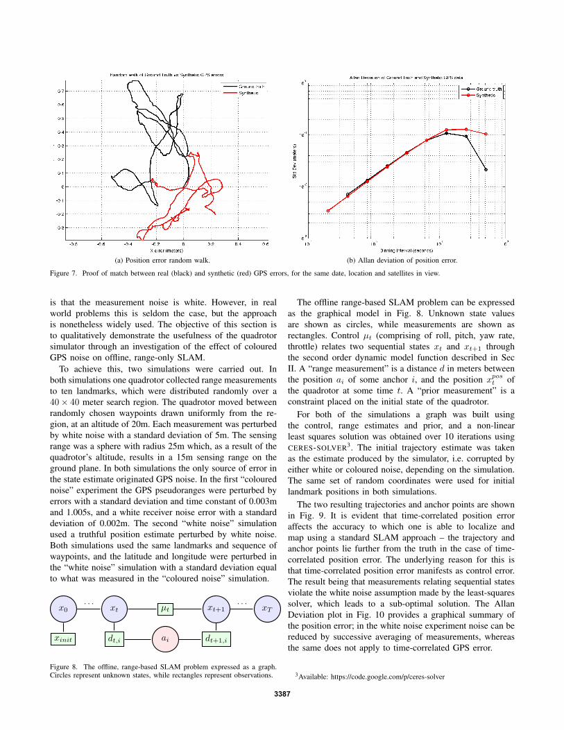
(a) Position error random walk. (b) Allan deviation of position error.

Figure 7. Proof of match between real (black) and synthetic (red) GPS errors, for the same date, location and satellites in view.

is that the measurement noise is white. However, in real

world problems this is seldom the case, but the approach

is nonetheless widely used. The objective of this section is

to qualitatively demonstrate the usefulness of the quadrotor

simulator through an investigation of the effect of coloured

GPS noise on offline, range-only SLAM.

To achieve this, two simulations were carried out. In

both simulations one quadrotor collected range measurements

to ten landmarks, which were distributed randomly over a

40× 40 meter search region. The quadrotor moved between

randomly chosen waypoints drawn uniformly from the re-

gion, at an altitude of 20m. Each measurement was perturbed

by white noise with a standard deviation of 5m. The sensing

range was a sphere with radius 25m which, as a result of the

quadrotor’s altitude, results in a 15m sensing range on the

ground plane. In both simulations the only source of error in

the state estimate originated GPS noise. In the first “coloured

noise” experiment the GPS pseudoranges were perturbed by

errors with a standard deviation and time constant of 0.003m

and 1.005s, and a white receiver noise error with a standard

deviation of 0.002m. The second “white noise” simulation

used a truthful position estimate perturbed by white noise.

Both simulations used the same landmarks and sequence of

waypoints, and the latitude and longitude were perturbed in

the “white noise” simulation with a standard deviation equal

to what was measured in the “coloured noise” simulation.

x0 xt µt xt+1

xinit dt,i ai dt+1,i

xT· · · · · ·

Figure 8. The offline, range-based SLAM problem expressed as a graph.Circles represent unknown states, while rectangles represent observations.

The offline range-based SLAM problem can be expressed

as the graphical model in Fig. 8. Unknown state values

are shown as circles, while measurements are shown as

rectangles. Control µt (comprising of roll, pitch, yaw rate,

throttle) relates two sequential states xt and xt+1 through

the second order dynamic model function described in Sec

II. A “range measurement” is a distance d in meters between

the position ai of some anchor i, and the position xpost of

the quadrotor at some time t. A “prior measurement” is a

constraint placed on the initial state of the quadrotor.

For both of the simulations a graph was built using

the control, range estimates and prior, and a non-linear

least squares solution was obtained over 10 iterations using

CERES-SOLVER3. The initial trajectory estimate was taken

as the estimate produced by the simulator, i.e. corrupted by

either white or coloured noise, depending on the simulation.

The same set of random coordinates were used for initial

landmark positions in both simulations.

The two resulting trajectories and anchor points are shown

in Fig. 9. It is evident that time-correlated position error

affects the accuracy to which one is able to localize and

map using a standard SLAM approach – the trajectory and

anchor points lie further from the truth in the case of time-

correlated position error. The underlying reason for this is

that time-correlated position error manifests as control error.

The result being that measurements relating sequential states

violate the white noise assumption made by the least-squares

solver, which leads to a sub-optimal solution. The Allan

Deviation plot in Fig. 10 provides a graphical summary of

the position error; in the white noise experiment noise can be

reduced by successive averaging of measurements, whereas

the same does not apply to time-correlated GPS error.

3Available: https://code.google.com/p/ceres-solver

3387

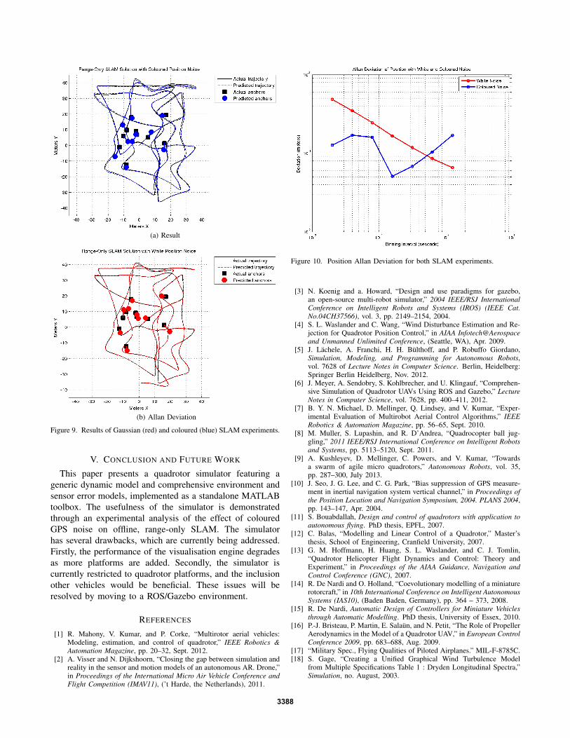
(a) Result

(b) Allan Deviation

Figure 9. Results of Gaussian (red) and coloured (blue) SLAM experiments.

V. CONCLUSION AND FUTURE WORK

This paper presents a quadrotor simulator featuring a

generic dynamic model and comprehensive environment and

sensor error models, implemented as a standalone MATLAB

toolbox. The usefulness of the simulator is demonstrated

through an experimental analysis of the effect of coloured

GPS noise on offline, range-only SLAM. The simulator

has several drawbacks, which are currently being addressed.

Firstly, the performance of the visualisation engine degrades

as more platforms are added. Secondly, the simulator is

currently restricted to quadrotor platforms, and the inclusion

other vehicles would be beneficial. These issues will be

resolved by moving to a ROS/Gazebo environment.

REFERENCES

[1] R. Mahony, V. Kumar, and P. Corke, “Multirotor aerial vehicles:Modeling, estimation, and control of quadrotor,” IEEE Robotics &

Automation Magazine, pp. 20–32, Sept. 2012.[2] A. Visser and N. Dijkshoorn, “Closing the gap between simulation and

reality in the sensor and motion models of an autonomous AR. Drone,”in Proceedings of the International Micro Air Vehicle Conference and

Flight Competition (IMAV11), (’t Harde, the Netherlands), 2011.

Figure 10. Position Allan Deviation for both SLAM experiments.

[3] N. Koenig and a. Howard, “Design and use paradigms for gazebo,an open-source multi-robot simulator,” 2004 IEEE/RSJ International

Conference on Intelligent Robots and Systems (IROS) (IEEE Cat.

No.04CH37566), vol. 3, pp. 2149–2154, 2004.[4] S. L. Waslander and C. Wang, “Wind Disturbance Estimation and Re-

jection for Quadrotor Position Control,” in AIAA Infotech@Aerospace

and Unmanned Unlimited Conference, (Seattle, WA), Apr. 2009.[5] J. Lächele, A. Franchi, H. H. Bülthoff, and P. Robuffo Giordano,

Simulation, Modeling, and Programming for Autonomous Robots,vol. 7628 of Lecture Notes in Computer Science. Berlin, Heidelberg:Springer Berlin Heidelberg, Nov. 2012.

[6] J. Meyer, A. Sendobry, S. Kohlbrecher, and U. Klingauf, “Comprehen-sive Simulation of Quadrotor UAVs Using ROS and Gazebo,” Lecture

Notes in Computer Science, vol. 7628, pp. 400–411, 2012.[7] B. Y. N. Michael, D. Mellinger, Q. Lindsey, and V. Kumar, “Exper-

imental Evaluation of Multirobot Aerial Control Algorithms,” IEEE

Robotics & Automation Magazine, pp. 56–65, Sept. 2010.[8] M. Muller, S. Lupashin, and R. D’Andrea, “Quadrocopter ball jug-

gling,” 2011 IEEE/RSJ International Conference on Intelligent Robots

and Systems, pp. 5113–5120, Sept. 2011.[9] A. Kushleyev, D. Mellinger, C. Powers, and V. Kumar, “Towards

a swarm of agile micro quadrotors,” Autonomous Robots, vol. 35,pp. 287–300, July 2013.

[10] J. Seo, J. G. Lee, and C. G. Park, “Bias suppression of GPS measure-ment in inertial navigation system vertical channel,” in Proceedings of

the Position Location and Navigation Symposium, 2004. PLANS 2004,pp. 143–147, Apr. 2004.

[11] S. Bouabdallah, Design and control of quadrotors with application to

autonomous flying. PhD thesis, EPFL, 2007.[12] C. Balas, “Modelling and Linear Control of a Quadrotor,” Master’s

thesis, School of Engineering, Cranfield University, 2007.[13] G. M. Hoffmann, H. Huang, S. L. Waslander, and C. J. Tomlin,

“Quadrotor Helicopter Flight Dynamics and Control: Theory andExperiment,” in Proceedings of the AIAA Guidance, Navigation and

Control Conference (GNC), 2007.[14] R. De Nardi and O. Holland, “Coevolutionary modelling of a miniature

rotorcraft,” in 10th International Conference on Intelligent Autonomous

Systems (IAS10), (Baden Baden, Germany), pp. 364 – 373, 2008.[15] R. De Nardi, Automatic Design of Controllers for Miniature Vehicles

through Automatic Modelling. PhD thesis, University of Essex, 2010.[16] P.-J. Bristeau, P. Martin, E. Salaün, and N. Petit, “The Role of Propeller

Aerodynamics in the Model of a Quadrotor UAV,” in European Control

Conference 2009, pp. 683–688, Aug. 2009.[17] “Military Spec., Flying Qualities of Piloted Airplanes.” MIL-F-8785C.[18] S. Gage, “Creating a Unified Graphical Wind Turbulence Model

from Multiple Specifications Table 1 : Dryden Longitudinal Spectra,”Simulation, no. August, 2003.

3388