Robust Optimal Control of Quadrotor UAVs

Received February 13, 2013, accepted April 16, 2013, published May 10, 2013.

Digital Object Identifier 10.1109/ACCESS.2013.2260794

Robust Optimal Control of Quadrotor UAVsAYKUT C. SATICI1, HASAN POONAWALA1, AND MARK W. SPONG1,21University of Texas at Dallas, Richardson, TX 75080, USA2Erik Jonsson School of Engineering and Computer Science, University of Texas at Dallas, Richardson, TX 75080, USA

Corresponding author: A. C. Satici ([email protected])

This work was supported in part by the National Science Foundation under Grants ECCS 07-25433 and CMMI-0856368, the University ofTexas STARs Program, and DGIST R&D Program of the Ministry of Education, Science and Technology of Korea under Grant12-BD-0101.

ABSTRACT This paper provides the design and implementation of an L1-optimal control of a quadrotorunmanned aerial vehicle (UAV). The quadrotor UAV is an underactuated rigid body with four propellersthat generate forces along the rotor axes. These four forces are used to achieve asymptotic tracking of fouroutputs, namely the position of the center of mass of the UAV and the heading. With perfect knowledgeof plant parameters and no measurement noise, the magnitudes of the errors are shown to exponentiallyconverge to zero. In the case of parametric uncertainty and measurement noise, the controller yields anexponential decrease of the magnitude of the errors in an L1-optimal sense. In other words, the controller isdesigned so that it minimizes the L∞-gain of the plant with respect to disturbances. The performance of thecontroller is evaluated in experiments and compared with that of a related robust nonlinear controller in theliterature. The experimental data shows that the proposed controller rejects persistent disturbances, which isquantified by a very small magnitude of the mean error.

INDEX TERMS Robust control, optimal control, quadrotor, feedback linearization, unmanned aerial vehicle.

I. INTRODUCTIONQuadrotors have become increasingly popular in recent yearsdue to their ability to hover and maneuver in tight spaces.Stabilizing the quadrotor in its configuration space SE(3) isan interesting and challenging control problem. The challengearises due to the availability of four control inputs to stabi-lize the system that lives in a six dimensional configurationspace and possesses coupled, nonlinear and unstable open-loop dynamics.

The goal of most quadrotor control schemes is either tostabilize the center of mass (CoM) at a desired location orfor the CoM to track a desired trajectory. Practical imple-mentation of these nonlinear control schemes for roboticsystems requires one to take into consideration the issues ofrobustness to parameter uncertainty, external disturbances,and sensor noise. It is well-known that the equations ofmotion of a quadrotor can be partially linearized [1] anddecoupled by appropriate nonlinear feedback. known as themethod of partial feedback linearization. It is very usefulfrom a control viewpoint, since a part of the complex highlycoupled nonlinear dynamics of the quadrotor are replaced bya simple set of second-order linear differential equations. Thepartial feedback linearization results in a controller that hasthe same order of complexity as the model of the system

being controlled. Good control performance requires a highsampling rate at which the desired control can be computed.A desire to maximize quadrotor payloads and performanceresults in a constraint on computational power available forautonomous control. It is highly advantageous therefore toconsider nonlinear feedback based upon simplified modelsand to quantify the performance of such controllers.In this paper the partial feedback linearization method

is applied to the nominal model. A linear compensator forthe resulting partial linear model is then designed using themethod of stable factorizations. The advantages of this controlscheme can be summarized as follows.

• Any linear compensator that stabilizes a linear modelcan be specified using the method of stable factoriza-tion. As a consequence, one is able to conclude whethera compensator designed based on the linear model isable to stabilize the ‘‘true’’ nonlinear system as well,provided the deviation between the modeled and theactual plant satisfies certain bounds.

• If the deviation of the model from the plant does notexceed themaximum allowable, it is possible to achievecorresponding reductions in the effects on the closed-loop performance of the parameter uncertainty, mea-surement noise, available computational power, etc.

VOLUME 1, 2013 2169-3536/$31.00 2013 IEEE 79

A. C. SATICI et al.: Robust Optimal Control of Quadrotor UAVs

The simplest control method involves linearization of thequadrotor dynamics around the hover state and then usingvarious linear control methods to stabilize the system, suchas standard SISO tools in [2], or PID and LQR methodsin [3]. In [4] the authors use a sliding mode control methodto stabilize the linearized dynamics. The work includes a ratelimited PID for control of the height. Controllers designedusing such linear methods may be used to track slowmotions.However, nonlinear control methods are needed to achievehigher performance and to execute more aggressive motions.

The quadrotor dynamics has a cascade structure. The fourmotor inputs are mapped to three independent torques actingon the quadrotor frame and one thrust force. The torqueinputs directly control the orientation dynamics. The orien-tation then affects the thrust vector direction which drives thetranslation dynamics. This cascade structure can be elegantlyexploited by using backstepping control techniques [5], [6] orinner-loop/outer-loop approaches [2], [3], [7]. Thework in [5]modifies the backstepping approach by using sliding modecontrol for one of the cascaded variables, which introducessome robustness to disturbances.

While the position of the CoM is almost always expressedin cartesian coordinates, selection of a representation for theorientation is an important step. All the papers mentioned sofar use an Euler-angle parametrization, which suffers fromsingularities. To address this, the work in [8] representsthe orientation using the rotation matrix itself. This leadsto an orientation tracking controller that is almost globallyattractive. The desired orientation and thrust magnitude aredesigned such that the translation dynamics are linear. Thepaper gives a good summary of the various representations.The samemethodwas implemented in the work of [9] in orderto achieve aggressive motions of a quadrotor.

Feedback linearization [10] is often employed in order tofacilitate the use of linear control methods over a large regionof the state space. The choice for the outputs or states tolinearizemay differ. In [11] the position and heading are takenas the outputs to be linearized whereas in [12] the height andthree Euler angles are linearized. The control inputs to thelinearized dynamics are selected as PD control.

Most nonlinear control methods are highly dependenton the exact knowledge of the system parameters inorder to achieve asymptotic tracking. Various researchershave attempted to address this issue using robust control[13]–[15] or adaptive control [16] and even a combination ofthe two [17]. The performance recovery generally trades offasymptotic stability with uniform ultimate boundedness.

The control method proposed in this paper also uses theidea of controlling the thrust direction to achieve positioncontrol. However, the control of orientation is prone to per-sistent disturbances stemming from uncertain inertial param-eters, misalignment of blade axes, discrepancy between themeasured quadrotor frame and the actual frame. The rejectionof such persistent disturbances is the primary motivation forour control design. Methods addressing this issue were firstdeveloped in [18]–[21].

The method in [21] elegantly determines the optimal lin-ear controller that stabilizes a given plant while rejectingpersistent disturbances. The method relies on the stable fac-torization approach [22] which is applicable only to linearplants. This precludes the methods used in [8] to stabilize thequadrotor since the plant remains nonlinear. The key contri-bution of this work is the parametrization of the orientationand subsequent partial feedback linearization of the dynamicswhich paves the way for applying the L1 optimal robust linearcompensator design for nonlinear robotic systems similarto [20]. Furthermore, we have implemented this controller ona quadrotor in LARS1 at the University of Texas at Dallas,and we have compared the performance of our controller withthat in [15]. The design of the robust controller in [15] is notbest suited for rejecting persistent disturbances, whereas ourcontroller is. The results show that our controller can handlethe effect of modeling errors such as blade misalignment andshifted center of mass location better than that in [15].

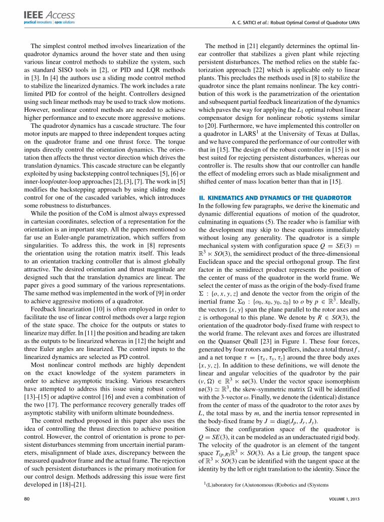
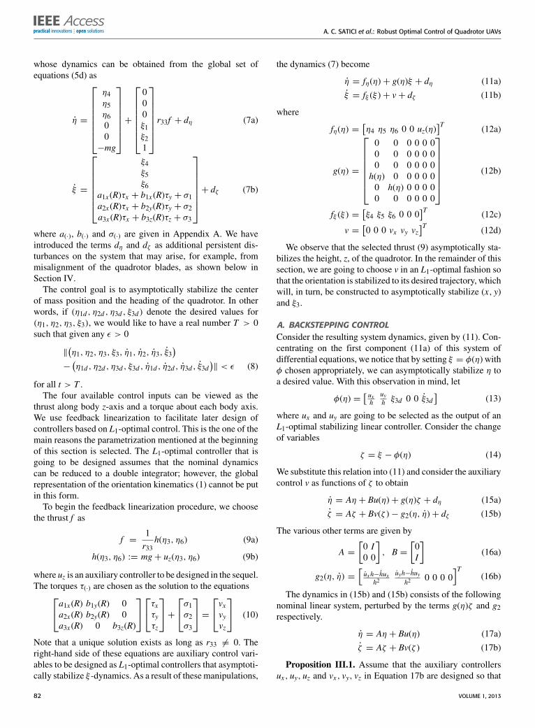
II. KINEMATICS AND DYNAMICS OF THE QUADROTORIn the following few paragraphs, we derive the kinematic anddynamic differential equations of motion of the quadrotor,culminating in equations (5). The reader who is familiar withthe development may skip to these equations immediatelywithout losing any generality. The quadrotor is a simplemechanical system with configuration space Q = SE(3) =R3 n SO(3), the semidirect product of the three-dimensionalEuclidean space and the special orthogonal group. The firstfactor in the semidirect product represents the position ofthe center of mass of the quadrotor in the world frame. Weselect the center of mass as the origin of the body-fixed frame6 : {o, x, y, z} and denote the vector from the origin of theinertial frame 60 : {o0, x0, y0, z0} to o by p ∈ R3. Ideally,the vectors {x, y} span the plane parallel to the rotor axes andz is orthogonal to this plane. We denote by R ∈ SO(3), theorientation of the quadrotor body-fixed frame with respect tothe world frame. The relevant axes and forces are illustratedon the Quanser Qball [23] in Figure 1. These four forces,generated by four rotors and propellers, induce a total thrust f ,and a net torque τ = {τx , τy, τz} around the three body axes{x, y, z}. In addition to these definitions, we will denote thelinear and angular velocities of the quadrotor by the pair(v, �) ∈ R3 n so(3). Under the vector space isomorphismso(3) ' R3, the skew-symmetric matrix � will be identifiedwith the 3-vectorω. Finally, we denote the (identical) distancefrom the center of mass of the quadrotor to the rotor axes byL, the total mass by m, and the inertia tensor represented inthe body-fixed frame by J = diag(Jp, Jr , Jy).

Since the configuration space of the quadrotor isQ = SE(3), it can be modeled as an underactuated rigid body.The velocity of the quadrotor is an element of the tangentspace T(p,R)R3 n SO(3). As a Lie group, the tangent spaceof R3 n SO(3) can be identified with the tangent space at theidentity by the left or right translation to the identity. Since the

1(L)aboratory for (A)utonomous (R)obotics and (S)ystems

80 VOLUME 1, 2013


FIGURE 1. Quanser Qball model.

rotational equations of motion are easier when expressedin the body-fixed frame, we choose to left translate to theidentity, which yields the body-fixed angular velocity

� = RT R (1)

Since the tangent space of R3 is again R3, the kinematics ofthe translational motion is simply v = p.The unforced translational dynamics of the quadrotor is the

same as the dynamics of a particle (center of mass) underthe action of the gravitational potential field. The total thrustf =

∑4i=1 fi acts on the acceleration of this particle in the

direction of the z-axis.The unforced rotational dynamics of the quadrotor are

given by the Lie-Poisson equations of motion of so(3)∗ rel-ative to the rigid body bracket. Following [24], we define theangular momentum in the body frame 5 := J� whence thekinetic energy function on so(3)∗ becomes

K (5) =125T J−15 (2)

Define another set of functionsFi(5) := 5i, i = {1, 2, 3}. SetF to be the vector-valued function with components Fi andapply the Lie-Poisson equations,

F = {F,K } (3a)

5 = −5 · (∇F(5)×∇K (5)) (3b)

= 5× J−15 (3c)

Expressing these equations in body angular velocities andincluding the body torques applied by the rotors,

J ω = Jω × ω + τ (4)

In summary, we have the following equations of motion forthe quadrotor describing the states at each instant in time.

p = v (5a)

mv = (−mg+ f R)e3 (5b)

R = R� (5c)

J ω = Jω × ω + τ (5d)

where e3 is the third standard unit vector in the Cartesiancoordinate system and g is the constant gravitational accel-eration. We have already mentioned that the total thrust isthe sum of the individual forces of the propellers. Sincethe front, back and left, right propellers rotate in oppositedirections, they generate a net torque around the z axis. Whilethe moment arm L and the difference between the forcesf1 and f3 generate a net torque around the y-axis, the differencebetween the forces f2 and f4 generate a net torque around thex-axis. This is summarized with the matrix equation givenbelow

fτx

τy

τz

=

1 1 1 10 −L 0 LL 0 −L 0Kτ Kτ −Kτ −Kτ

f1f2f3f4

. (6)

III. CONTROL DESIGNWe parametrize the 12-dimensional state space of the quadro-tor by selecting six position variables and their time deriva-tives. The first three position variables (x, y, z) specify thecenter of mass, p, of the quadrotor, while the remainingthree position variables

(r13r33,r23r33, arctan2 (−r12, r22)

)spec-

ify the orientation of the quadrotor with respect to theinertial frame. The numbers rij are the elements of therotation matrix R ∈ SO(3). The parametrization of the ori-entation is local and restricted to the connected open subsetU = {R ∈ SO(3) : r33 > 0} of SO(3). The first two orien-tation variables are proportional to the x and y componentsof the thrust vector in the world frame determining the linearhorizontal acceleration of the quadrotor in this frame. The lastorientation variable corresponds to the heading of the bodyx-axis in the world frame, which can also be interpretedas the yaw angle in a Body312 Euler angle representa-tion of the orientation. Unlike the traditional Euler-angleparametrization, the orientation variables in our parametriza-tion above enter linearly in the translation dynamics, asshown below, which facilitates the corresponding controllerdevelopment.In this parametrization of the state space, a point is

specified by the vectors

η = (η1, . . . , η6)T= (x, y, z, x, y, z)T

ξ = (ξ1, . . . , ξ6)T

where

ξ1 =r13r33, ξ2 =

r13r33

ξ3 = arctan2 (−r12, r22), ξ4 =r13r33 − r13r33

r233

ξ5 =r23r33 − r23r33

r233, ξ6 =

r22r12 − r22r12r212 + r

222

VOLUME 1, 2013 81


whose dynamics can be obtained from the global set ofequations (5d) as

η =

η4η5η600−mg

+000ξ1ξ21

r33f + dη (7a)

ξ =

ξ4ξ5ξ6

a1x(R)τx + b1x(R)τy + σ1a2x(R)τx + b2y(R)τy + σ2a3x(R)τx + b3z(R)τz + σ3

+ dζ (7b)

where a(·), b(·) and σ(·) are given in Appendix A. We haveintroduced the terms dη and dζ as additional persistent dis-turbances on the system that may arise, for example, frommisalignment of the quadrotor blades, as shown below inSection IV.

The control goal is to asymptotically stabilize the centerof mass position and the heading of the quadrotor. In otherwords, if (η1d , η2d , η3d , ξ3d ) denote the desired values for(η1, η2, η3, ξ3), we would like to have a real number T > 0such that given any ε > 0

‖(η1, η2, η3, ξ3, η1, η2, η3, ξ3

)−(η1d , η2d , η3d , ξ3d , η1d , η2d , η3d , ξ3d

)‖ < ε (8)

for all t > T .The four available control inputs can be viewed as the

thrust along body z-axis and a torque about each body axis.We use feedback linearization to facilitate later design ofcontrollers based on L1-optimal control. This is the one of themain reasons the parametrization mentioned at the beginningof this section is selected. The L1-optimal controller that isgoing to be designed assumes that the nominal dynamicscan be reduced to a double integrator; however, the globalrepresentation of the orientation kinematics (1) cannot be putin this form.

To begin the feedback linearization procedure, we choosethe thrust f as

f =1r33

h(η3, η6) (9a)

h(η3, η6) := mg+ uz(η3, η6) (9b)

where uz is an auxiliary controller to be designed in the sequel.The torques τ(·) are chosen as the solution to the equationsa1x(R) b1y(R) 0

a2x(R) b2y(R) 0a3x(R) 0 b3z(R)

τxτyτz

+σ1σ2σ3

=vxvyvz

(10)

Note that a unique solution exists as long as r33 6= 0. Theright-hand side of these equations are auxiliary control vari-ables to be designed as L1-optimal controllers that asymptoti-cally stabilize ξ -dynamics. As a result of these manipulations,

the dynamics (7) become

η = fη(η)+ g(η)ξ + dη (11a)

ξ = fξ (ξ )+ v+ dζ (11b)

where

fη(η) =[η4 η5 η6 0 0 uz(η)

]T (12a)

g(η) =

0 0 0 0 0 00 0 0 0 0 00 0 0 0 0 0h(η) 0 0 0 0 00 h(η) 0 0 0 00 0 0 0 0 0

(12b)

fξ (ξ ) =[ξ4 ξ5 ξ6 0 0 0

]T (12c)

v =[0 0 0 vx vy vz

]T (12d)

We observe that the selected thrust (9) asymptotically sta-bilizes the height, z, of the quadrotor. In the remainder of thissection, we are going to choose v in an L1-optimal fashion sothat the orientation is stabilized to its desired trajectory, whichwill, in turn, be constructed to asymptotically stabilize (x, y)and ξ3.

A. BACKSTEPPING CONTROLConsider the resulting system dynamics, given by (11). Con-centrating on the first component (11a) of this system ofdifferential equations, we notice that by setting ξ = φ(η) withφ chosen appropriately, we can asymptotically stabilize η toa desired value. With this observation in mind, let

φ(η) =[ uxh

uyh ξ3d 0 0 ξ3d

](13)

where ux and uy are going to be selected as the output of anL1-optimal stabilizing linear controller. Consider the changeof variables

ζ = ξ − φ(η) (14)

We substitute this relation into (11) and consider the auxiliarycontrol v as functions of ζ to obtain

η = Aη + Bu(η)+ g(η)ζ + dη (15a)

ζ = Aζ + Bv(ζ )− g2(η, η)+ dζ (15b)

The various other terms are given by

A =[0 I0 0

], B =

[0I

](16a)

g2(η, η) =[uxh−hux

h2uyh−huy

h20 0 0 0

]T(16b)

The dynamics in (15b) and (15b) consists of the followingnominal linear system, perturbed by the terms g(η)ζ and g2respectively.

η = Aη + Bu(η) (17a)

ζ = Aζ + Bv(ζ ) (17b)

Proposition III.1. Assume that the auxiliary controllersux , uy, uz and vx , vy, vz in Equation 17b are designed so that

82 VOLUME 1, 2013


the origin of (17b) is exponentially stable. Then, when thedisturbance terms dη and dζ are zero, the origin of the fullsystem 15b is exponentially stable.

Proof: It suffices to show that the perturbation terms in (15)are locally Lipschitz and vanish at the origin (η, ζ ) ≡ (0, 0).This is trivially true for the term g(η)ζ as g(η) is bounded andis continuously differentiable. On the other hand, the secondterm g2(η, η), is comprised of the time derivative of ux

h anduyh . Notice that all of these functions are at least continuouslydifferentiable functions of (η, η) and therefore, are locallyLipschitz. Moreover, since ux , uy are linear functions and h isan affine function of η, the functions ux

h and uyh are identically

zerowhenever η is identically zero. This, in particular, impliesthat under these circumstances, the time derivative of thesefunctions are also identically zero.

From this analysis, we can conclude by [10, p. 341,Lemma 9.1] that the origin of the perturbed system (15) isexponentially stable.Remark 1. In purely model inversion techniques, in order

to feedback linearize equation (15) one would require knowl-edge of g2. However, the computation of g2 is not feasiblesince it requires acceleration level measurements, which areknown to be extremely noisy. In contrast, proposition III-Ameans that to achieve exponential stability we do not need touse this malevolent signal in our control law.

B. L1 OPTIMAL CONTROLIn this section, we present our main result, which is the designof the control inputs u(η) and v(ζ ) for the system (15) usingthe L1-optimal control design procedure from [20] and [21].

We first use the stable factorization approach, given anexposition in [22], that allows one to parametrize the set ofall controllers that stabilize a given (linear) system as well asthe set of all stable transfer matrices that are achievable.

The first step of the approach is to factor the plant transfermatrix G into a ‘‘ratio’’ of the form

G(s) = N (s) [D(s)]−1 =[D(s)

]−1N (s) (18)

where N , D, N , D are stable rational matrices, i.e., everyelement of each matrix is proper and has all of its poles inthe open left half-plane. Next, one solves the so-called Bezoutidentities: [

Y (s) X (s)−N (s) D(s)

] [D(s) −X (s)N (s) Y (s)

]= I (19)

where X , X , Y , Y are also stable rational matrices. It can thenbe shown that the set of all controllers that stabilize G is givenby [22] {

−

(Y − RN

)−1 (X + RD

)}(20)

where R is an arbitrary matrix of appropriate dimensionswhose elements are stable rational functions.

We notice that the nominal plant G(s) of equation (18)given by (17) is a system of double integrators. It is then

routine to determine the various other matrices in (18) and(19) using the techniques of [25]. This gives

G(s) =1s2

[IsI

](21a)

N (s) = N (s) =1

(s+ 1)2

[IsI

](21b)

D(s) =s2

(s+ 1)2· I (21c)

D(s) =1

(s+ 1)2

[(s2 + 2s)I −2I−sI (s2 + 1)I

](21d)

X (s) = X (s) =1

(s+ 1)2[1+ 2s 2+ 4s

]I (21e)

Y (s) =s2 + 4s+ 2(s+ 1)2

· I (21f)

Y (s) =1

(s+ 1)2

[(s2 + 2s+ 2)I 2I

sI (s2 + 4s+ 1)I

](21g)

It is shown in [20] how to choose the ‘‘free’’ parameter R in(20) such that the system error rejects ‘‘uncertainties’’ due tosystem modeling. Thus, the only error that may remain willbe due to the measurement noise. The procedure involves pro-ducing a sequence {Rk} and examining the resulting controller

Ck = −(Y − Rk N

)−1 (X + Rk D

)(22)

and the error dynamics

e = P1kζ + P2kw (23)

where ζ stands for all the persistent disturbances exerted onthe system (15), w denotes the measurement error, and thetransfer matrices P1k and P2k are given by

P1k = N (Y − Rk N ) (24a)

P2k = I − D(Y − Rk N ) (24b)

The sequence {Rk} in the linear compensator expression (22)can be chosen such that as k → ∞, ‖P1k‖A → 0 and‖P2k‖A → 1, with the A norm denoting the L∞-gain ofthe system Pi. As ‖P1k‖A → 0, the rejection of persistentdisturbances gets better and better. Since minimizing theL∞-gain of the operator Pi minimizes the L1-gain of the inputsignal, this procedure amounts to designing an L1-optimalcontroller for the quadrotor. This implies that in the absenceof measurement noise, the mean value of the error over timewill be minimized.

The linear controllers consist of two different transferfunctions that accept position and velocity errors as inputs,respectively. Each yields control forces/torques that are addedtogether to form the final linear controller. The forms of theresulting linear controllers derived using this robust controlframework are given below.

U (s)Ep(s)

=2k1s2 + k1k2s+ k21

s2(25a)

U (s)Ev(s)

=2k2s2 + k22 s+ k1k2

s2(25b)

VOLUME 1, 2013 83


where k1 and k2 positive are gains to be tuned. The tuningprocess is not so difficult to achieve once it is noted thatk1 acts as the proportional (spring) and k2 as the deriva-tive (damping) gain of the system. Each of the controllers{ux , uy, uz, vx , vy, vz} mentioned in the Section III-A are ofthis form with appropriately chosen k1, k2 gains. Particularchoices of these gains, suited for our quadrotor, are given inSection IV.

IV. SIMULATION RESULTSThis section presents simulations of the proposed (LARS)controller on a model of the Quanser Qball quadrotor [23]taking into account the various sources of modeling uncer-tainties. The controller is compared with that presented in [8],which we refer to as RGTC standing for ‘‘Robust GeometricTracking Controller’’. The simulations are required in orderto demonstrate performance for the case when only modeluncertainty is present, whereas in experiment some measure-ment noise is present. We also present simulations whichinclude measurement noise in the model. The Quanser Qballhas the following properties as given in its user manual:

J = diag ([0.03, 0.03, 0.03]) kg ·m2 (26a)

m = 1.4 kg, ω = 15radsec

(26b)

where ω is the actuator bandwidth of each propeller. That is,the force output of each propeller is achieved by passing thecommand through a low-pass filter with 15

2πHz. bandwidth.This, of course, is a huge limitation on the range fast ofmotions achievable. Therefore, we design a simple lead con-troller that moves the pole at ω = 15

2πHz to37.52π Hz. This mini

controller can be expressed in frequency domain as

F(s)U (s)

= C(s) = 2.5s+ 15s+ 37.5

(27)

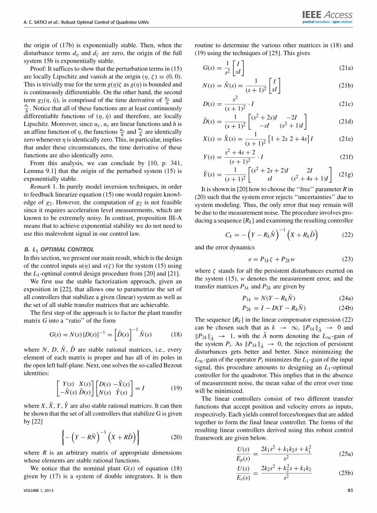
The quadrotor is subject to several kinds of uncertainties,the most straightforward of which are its mass and its inertiatensor. More subtle uncertainties include misalignment of therotors with respect to the quadrotor frame. That is, althoughthe rotors of the blades are supposed to be parallel to theframe of the quadrotor, in reality, they might be slightly tiltedcausing the application of unmodeled forces and moments onthe quadrotor. Such rotor misalignment has been observedon the quadrotor in our laboratory. Moreover, if the centerof mass of the quadrotor is not located exactly at the center,the manner in which the torques enter into the rotationaldynamics is no longer given by (6). The visualization of the‘‘actual’’ quadrotor in Figure 2 sheds light on the derivation ofits ‘‘actual’’ dynamics. In this figure, we see that the plane ofthe quadrotor frame, P, has a normal vector N . In the idealmodel, the forces of each of the propellers are along thisnormal. The direction of these forces deviate from this normalin reality, as depicted in Figure 2, giving rise to the dynamicalequations of motion presented in (28)

FIGURE 2. ‘‘Actual’’ Quadrotor Model: The direction of the thrust forces ofeach of the propellers deviate from the normal vector to the plane of thequadrotor frame. The CoM is not exactly situated at the center of thequadrotor frame.

J ω + ω × Jω =4∑i=1

fi[Kτσ (i)I + pi

]Ri · e3 (28a)

mp =4∑i=4

(−mgI + fiRi) · e3 (28b)

where Ri ∈ SO(3) is the orientation of the ith propellerwith respect to the quadrotor frame, e3 is the third standardCartesian unit vector, pi is the position vector, in the quadrotorframe, from the center of mass C to the center of the ith

propeller. The hat operator ˆ is the usual isomorphism fromR3 to so(3). Lastly, I is the 3 × 3 identity matrix and σ :{1, 2, 3, 4} → {−1, 1} is defined by

σ (i) =

{1 if i = 1, 2−1 if i = 3, 4

The experimentally determined values of Rie3 for the fourrotors are given by

R1e3 =[0.03 0.03 0.9991

]T (29a)

R2e3 =[0.06 0.03 0.9977

]T (29b)

R3e3 =[0.03 0.06 0.9977

]T (29c)

R4e3 =[0.09 0.09 0.9919

]T (29d)

Finally, the measurements of the quadrotor pose and veloc-ity are never perfect. In the simulations, they will be modeledas a Gaussian noise acting on both the linear and angularreadings additively. In what follows, we are going to presentsimulation results of our proposed controller and compareit with one of the most prominent robust controllers in theliterature provided by [15].The value of gain parameters used in our controller is

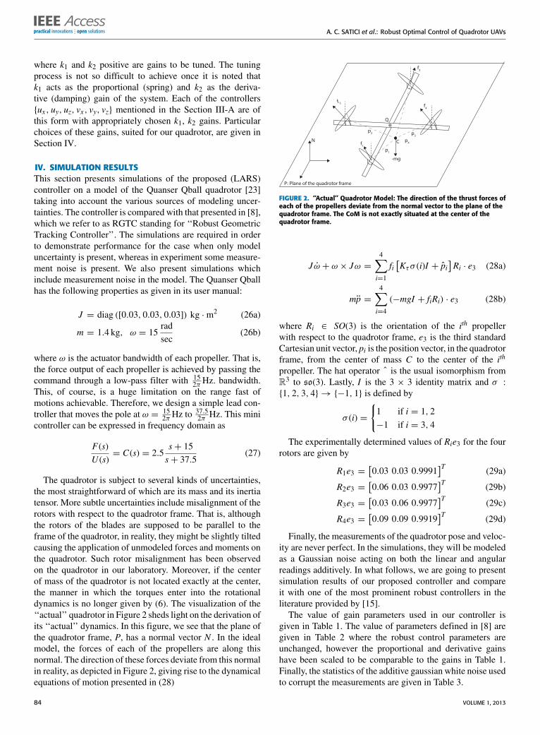
given in Table 1. The value of parameters defined in [8] aregiven in Table 2 where the robust control parameters areunchanged, however the proportional and derivative gainshave been scaled to be comparable to the gains in Table 1.Finally, the statistics of the additive gaussian white noise usedto corrupt the measurements are given in Table 3.

84 VOLUME 1, 2013


TABLE 1. Gains used in our controller.

Loop k1 k2x 3 3.4293

y 3 2.6944

z 3 2.6944

ξ1 176.2000 26.5481

ξ2 176.2000 26.5481

ξ3 26.4300 10.2820

TABLE 2. Parameters from [8].

Parameter Value

KR 5.3394 I3K� 0.7

kx 6

kv 5.4

c1 3.6

c2 0.6

εx 0.04

εR 0.04

TABLE 3. Variances of additive zero mean gaussian white noise.

Parameter Value

σ 2p 10−6

σ 2p 0.01

σ 2R 10−4

σ 2ω 0.01

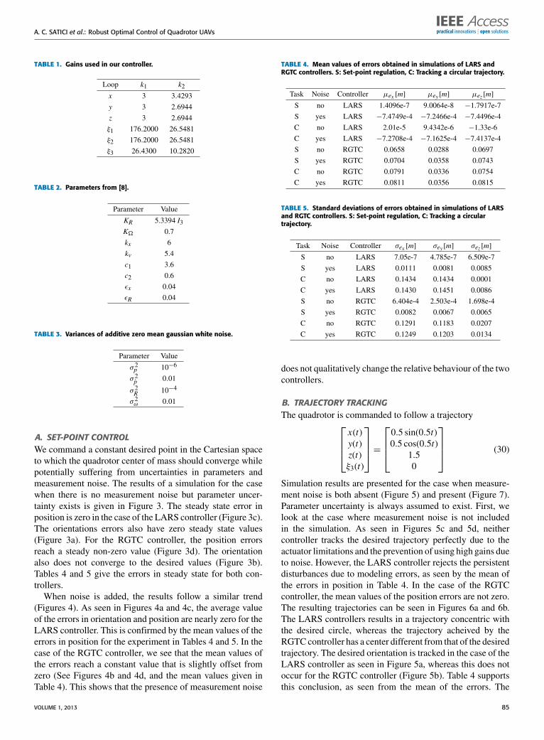
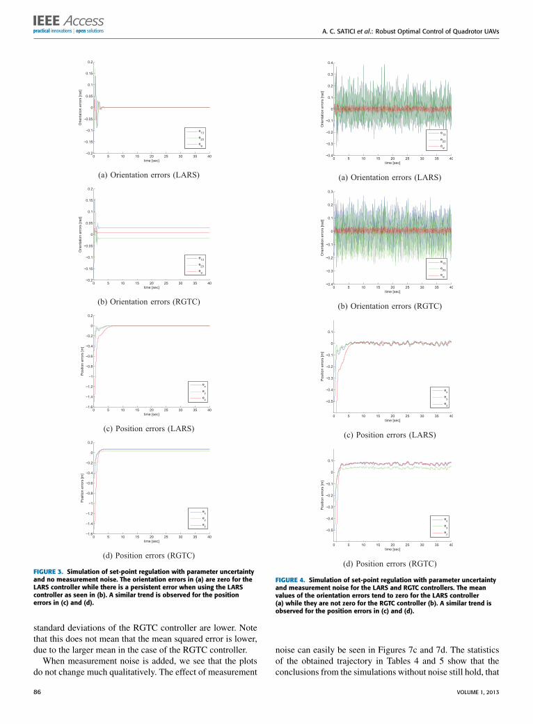
A. SET-POINT CONTROLWe command a constant desired point in the Cartesian spaceto which the quadrotor center of mass should converge whilepotentially suffering from uncertainties in parameters andmeasurement noise. The results of a simulation for the casewhen there is no measurement noise but parameter uncer-tainty exists is given in Figure 3. The steady state error inposition is zero in the case of the LARS controller (Figure 3c).The orientations errors also have zero steady state values(Figure 3a). For the RGTC controller, the position errorsreach a steady non-zero value (Figure 3d). The orientationalso does not converge to the desired values (Figure 3b).Tables 4 and 5 give the errors in steady state for both con-trollers.

When noise is added, the results follow a similar trend(Figures 4). As seen in Figures 4a and 4c, the average valueof the errors in orientation and position are nearly zero for theLARS controller. This is confirmed by the mean values of theerrors in position for the experiment in Tables 4 and 5. In thecase of the RGTC controller, we see that the mean values ofthe errors reach a constant value that is slightly offset fromzero (See Figures 4b and 4d, and the mean values given inTable 4). This shows that the presence of measurement noise

TABLE 4. Mean values of errors obtained in simulations of LARS andRGTC controllers. S: Set-point regulation, C: Tracking a circular trajectory.

Task Noise Controller µex [m] µey [m] µez [m]

S no LARS 1.4096e-7 9.0064e-8 −1.7917e-7

S yes LARS −7.4749e-4 −7.2466e-4 −7.4496e-4

C no LARS 2.01e-5 9.4342e-6 −1.33e-6

C yes LARS −7.2708e-4 −7.1625e-4 −7.4137e-4

S no RGTC 0.0658 0.0288 0.0697

S yes RGTC 0.0704 0.0358 0.0743

C no RGTC 0.0791 0.0336 0.0754

C yes RGTC 0.0811 0.0356 0.0815

TABLE 5. Standard deviations of errors obtained in simulations of LARSand RGTC controllers. S: Set-point regulation, C: Tracking a circulartrajectory.

Task Noise Controller σex [m] σey [m] σez [m]

S no LARS 7.05e-7 4.785e-7 6.509e-7

S yes LARS 0.0111 0.0081 0.0085

C no LARS 0.1434 0.1434 0.0001

C yes LARS 0.1430 0.1451 0.0086

S no RGTC 6.404e-4 2.503e-4 1.698e-4

S yes RGTC 0.0082 0.0067 0.0065

C no RGTC 0.1291 0.1183 0.0207

C yes RGTC 0.1249 0.1203 0.0134

does not qualitatively change the relative behaviour of the twocontrollers.

B. TRAJECTORY TRACKINGThe quadrotor is commanded to follow a trajectory

x(t)y(t)z(t)ξ3(t)

=0.5 sin(0.5t)0.5 cos(0.5t)

1.50

(30)

Simulation results are presented for the case when measure-ment noise is both absent (Figure 5) and present (Figure 7).Parameter uncertainty is always assumed to exist. First, welook at the case where measurement noise is not includedin the simulation. As seen in Figures 5c and 5d, neithercontroller tracks the desired trajectory perfectly due to theactuator limitations and the prevention of using high gains dueto noise. However, the LARS controller rejects the persistentdisturbances due to modeling errors, as seen by the mean ofthe errors in position in Table 4. In the case of the RGTCcontroller, the mean values of the position errors are not zero.The resulting trajectories can be seen in Figures 6a and 6b.The LARS controllers results in a trajectory concentric withthe desired circle, whereas the trajectory acheived by theRGTC controller has a center different from that of the desiredtrajectory. The desired orientation is tracked in the case of theLARS controller as seen in Figure 5a, whereas this does notoccur for the RGTC controller (Figure 5b). Table 4 supportsthis conclusion, as seen from the mean of the errors. The

VOLUME 1, 2013 85


0 5 10 15 20 25 30 35 40−0.2

−0.15

−0.1

−0.05

0

0.05

0.1

0.15

0.2

time [sec]

Orie

nta

tio

n e

rro

rs [ra

d]

e13

e23

eψ

(a) Orientation errors (LARS)

0 5 10 15 20 25 30 35 40−0.2

−0.15

−0.1

−0.05

0

0.05

0.1

0.15

0.2

time [sec]

Orie

nta

tio

n e

rro

rs [ra

d]

e13

e23

eψ

(b) Orientation errors (RGTC)

0 5 10 15 20 25 30 35 40−1.6

−1.4

−1.2

−1

−0.8

−0.6

−0.4

−0.2

0

0.2

time [sec]

Positio

n e

rro

rs [m

]

ex

ey

ez

(c) Position errors (LARS)

0 5 10 15 20 25 30 35 40−1.6

−1.4

−1.2

−1

−0.8

−0.6

−0.4

−0.2

0

0.2

time [sec]

Positio

n e

rro

rs [m

]

ex

ey

ez

(d) Position errors (RGTC)

FIGURE 3. Simulation of set-point regulation with parameter uncertaintyand no measurement noise. The orientation errors in (a) are zero for theLARS controller while there is a persistent error when using the LARScontroller as seen in (b). A similar trend is observed for the positionerrors in (c) and (d).

standard deviations of the RGTC controller are lower. Notethat this does not mean that the mean squared error is lower,due to the larger mean in the case of the RGTC controller.

When measurement noise is added, we see that the plotsdo not change much qualitatively. The effect of measurement

0 5 10 15 20 25 30 35 40−0.4

−0.3

−0.2

−0.1

0

0.1

0.2

0.3

0.4

time [sec]

Orienta

tion

err

ors

[ra

d]

e13

e23

eψ


0 5 10 15 20 25 30 35 40−0.4

−0.3

−0.2

−0.1

0

0.1

0.2

0.3

time [sec]

Orienta

tion

err

ors

[ra

d]

e13

e23

eψ


0 5 10 15 20 25 30 35 40

−0.5

−0.4

−0.3

−0.2

−0.1

0

0.1

time [sec]

Positio

n e

rrors

[m

]

ex

ey

ez


0 5 10 15 20 25 30 35 40

−0.5

−0.4

−0.3

−0.2

−0.1

0

0.1

time [sec]

Positio

n e

rrors

[m

]

ex

ey

ez


FIGURE 4. Simulation of set-point regulation with parameter uncertaintyand measurement noise for the LARS and RGTC controllers. The meanvalues of the orientation errors tend to zero for the LARS controller(a) while they are not zero for the RGTC controller (b). A similar trend isobserved for the position errors in (c) and (d).

noise can easily be seen in Figures 7c and 7d. The statisticsof the obtained trajectory in Tables 4 and 5 show that theconclusions from the simulations without noise still hold, that

86 VOLUME 1, 2013


0 5 10 15 20 25 30 35 40−0.2

−0.15

−0.1

−0.05

0

0.05

0.1

0.15

0.2

0.25

time [sec]

Orie

nta

tio

n e

rro

rs [

rad

]

e13

e23

eψ


0 5 10 15 20 25 30 35 40−0.2

−0.15

−0.1

−0.05

0

0.05

0.1

0.15

time [sec]

Orie

nta

tio

n e

rro

rs [

rad

]

e13

e23

eψ


0 5 10 15 20 25 30 35 40−1.6

−1.4

−1.2

−1

−0.8

−0.6

−0.4

−0.2

0

0.2

0.4

time [sec]

Positio

n e

rro

rs [m

]

ex

ey

ez


0 5 10 15 20 25 30 35 40−1.6

−1.4

−1.2

−1

−0.8

−0.6

−0.4

−0.2

0

0.2

0.4

time [sec]

Po

sitio

n e

rro

rs [m

]

ex

ey

ez


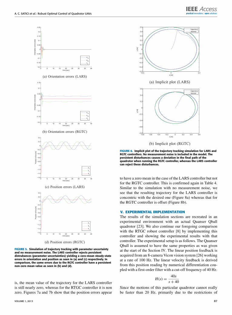
FIGURE 5. Simulation of trajectory tracking with parameter uncertaintyand no measurement noise. The LARS controller rejects persistentdistrubances (parameter uncertainties) yielding a zero-mean steady-stateerrors in orientation and position as seen in (a) and (c) respectively. Incomparison, the same errors due to the RGTC controller have a persistentnon-zero mean value as seen in (b) and (d).

is, the mean value of the trajectory for the LARS controlleris still nearly zero, whereas for the RTGC controller it is nonzero. Figures 7a and 7b show that the position errors appear

−0.5 0 0.5−0.5

−0.4

−0.3

−0.2

−0.1

0

0.1

0.2

0.3

0.4

0.5

x [m]

y [m

]

trajectory

desired

(a) Implicit plot (LARS)

−0.8 −0.6 −0.4 −0.2 0 0.2 0.4 0.6−0.8

−0.6

−0.4

−0.2

0

0.2

0.4

0.6

x [m]y [m

]

trajectory

desired

(b) Implicit plot (RGTC)

FIGURE 6. Implicit plot of the trajectory tracking simulation for LARS andRGTC controllers. No measurement noise is included in the model. Thepersistent disturbances causes a deviation in the final path of thequadrotor when running the RGTC controller, whereas the LARS controllercan reject these disturbances.

to have a zero mean in the case of the LARS controller but notfor the RGTC controller. This is confirmed again in Table 4.Similar to the simulation with no measurement noise, wesee that the resulting trajectory for the LARS controller isconcentric with the desired one (Figure 8a) whereas that forthe RGTC controller is offset (Figure 8b).

V. EXPERIMENTAL IMPLEMENTATIONThe results of the simulation sections are recreated in anexperimental environment with an actual Quanser Qballquadrotor [23]. We also continue our foregoing comparisonwith the RTGC robust controller [8] by implementing thiscontroller and showing the experimental results with thatcontroller. The experimental setup is as follows. The QuanserQball is assumed to have the same properties as was givenat the start of the Section IV. The linear position feedback isacquired from an 8-camera Vicon vision system [26] workingat a rate of 100 Hz. The linear velocity feedback is derivedfrom this position reading by numerical differentiation cou-pled with a first-order filter with a cut-off frequency of 40 Hz.

H (s) =40s

s+ 40

Since the motions of this particular quadrotor cannot reallybe faster than 20 Hz. primarily due to the restrictions of

VOLUME 1, 2013 87


0 5 10 15 20 25 30 35 40−1.6

−1.4

−1.2

−1

−0.8

−0.6

−0.4

−0.2

0

0.2

0.4

time [sec]

Positio

n e

rrors

[m

]

ex

ey

ez

(a) Position errors (LARS)

0 5 10 15 20 25 30 35 40−1.6

−1.4

−1.2

−1

−0.8

−0.6

−0.4

−0.2

0

0.2

0.4

time [sec]

ex

ey

ez

(b) Position errors (RGTC)

0 5 10 15 20 25 30 35 40−0.3

−0.2

−0.1

0

0.1

0.2

0.3

0.4

time [sec]

Orie

nta

tion e

rrors

[ra

d]

e13

e23

eψ

(c) Orientation errors (LARS)

0 5 10 15 20 25 30 35 40−0.4

−0.3

−0.2

−0.1

0

0.1

0.2

0.3

time [sec]

Orie

nta

tion e

rrors

[ra

d]

e13

e23

eψ

(d) Orientation errors (RGTC)

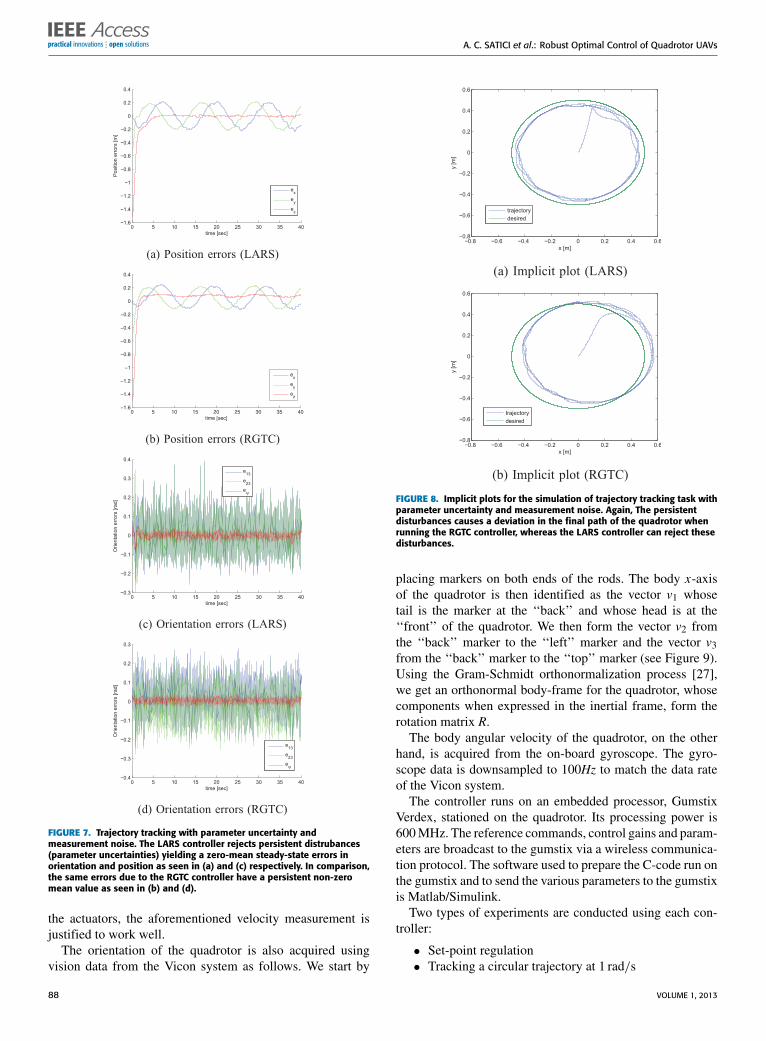
FIGURE 7. Trajectory tracking with parameter uncertainty andmeasurement noise. The LARS controller rejects persistent distrubances(parameter uncertainties) yielding a zero-mean steady-state errors inorientation and position as seen in (a) and (c) respectively. In comparison,the same errors due to the RGTC controller have a persistent non-zeromean value as seen in (b) and (d).

the actuators, the aforementioned velocity measurement isjustified to work well.

The orientation of the quadrotor is also acquired usingvision data from the Vicon system as follows. We start by

−0.8 −0.6 −0.4 −0.2 0 0.2 0.4 0.6−0.8

−0.6

−0.4

−0.2

0

0.2

0.4

0.6

x [m]

y [m

]

trajectory

desired


−0.8 −0.6 −0.4 −0.2 0 0.2 0.4 0.6−0.8

−0.6

−0.4

−0.2

0

0.2

0.4

0.6

x [m]y [m

]

trajectory

desired


FIGURE 8. Implicit plots for the simulation of trajectory tracking task withparameter uncertainty and measurement noise. Again, The persistentdisturbances causes a deviation in the final path of the quadrotor whenrunning the RGTC controller, whereas the LARS controller can reject thesedisturbances.

placing markers on both ends of the rods. The body x-axisof the quadrotor is then identified as the vector v1 whosetail is the marker at the ‘‘back’’ and whose head is at the‘‘front’’ of the quadrotor. We then form the vector v2 fromthe ‘‘back’’ marker to the ‘‘left’’ marker and the vector v3from the ‘‘back’’ marker to the ‘‘top’’ marker (see Figure 9).Using the Gram-Schmidt orthonormalization process [27],we get an orthonormal body-frame for the quadrotor, whosecomponents when expressed in the inertial frame, form therotation matrix R.The body angular velocity of the quadrotor, on the other

hand, is acquired from the on-board gyroscope. The gyro-scope data is downsampled to 100Hz to match the data rateof the Vicon system.The controller runs on an embedded processor, Gumstix

Verdex, stationed on the quadrotor. Its processing power is600MHz. The reference commands, control gains and param-eters are broadcast to the gumstix via a wireless communica-tion protocol. The software used to prepare the C-code run onthe gumstix and to send the various parameters to the gumstixis Matlab/Simulink.Two types of experiments are conducted using each con-

troller:

• Set-point regulation• Tracking a circular trajectory at 1 rad/s

88 VOLUME 1, 2013


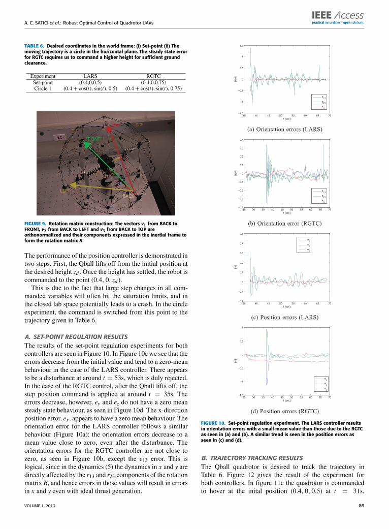
TABLE 6. Desired coordinates in the world frame: (i) Set-point (ii) Themoving trajectory is a circle in the horizontal plane. The steady state errorfor RGTC requires us to command a higher height for sufficient groundclearance.

Experiment LARS RGTCSet-point (0.4,0,0.5) (0.4,0,0.75)Circle 1 (0.4+ cos(t), sin(t), 0.5) (0.4+ cos(t), sin(t), 0.75)

FIGURE 9. Rotation matrix construction: The vectors v1 from BACK toFRONT, v2 from BACK to LEFT and v3 from BACK to TOP areorthonormalized and their components expressed in the inertial frame toform the rotation matrix R

The performance of the position controller is demonstrated intwo steps. First, the Qball lifts off from the initial position atthe desired height zd . Once the height has settled, the robot iscommanded to the point (0.4, 0, zd ).

This is due to the fact that large step changes in all com-manded variables will often hit the saturation limits, and inthe closed lab space potentially leads to a crash. In the circleexperiment, the command is switched from this point to thetrajectory given in Table 6.

A. SET-POINT REGULATION RESULTSThe results of the set-point regulation experiments for bothcontrollers are seen in Figure 10. In Figure 10c we see that theerrors decrease from the initial value and tend to a zero-meanbehaviour in the case of the LARS controller. There appearsto be a disturbance at around t = 53s, which is duly rejected.In the case of the RGTC control, after the Qball lifts off, thestep position command is applied at around t = 35s. Theerrors decrease, however, ey and ez do not have a zero meansteady state behaviour, as seen in Figure 10d. The x-directionposition error, ex , appears to have a zero mean behaviour. Theorientation error for the LARS controller follows a similarbehaviour (Figure 10a): the orientation errors decrease to amean value close to zero, even after the disturbance. Theorientation errors for the RGTC controller are not close tozero, as seen in Figure 10b, except the e13 error. This islogical, since in the dynamics (5) the dynamics in x and y aredirectly affected by the r13 and r23 components of the rotationmatrix R, and hence errors in those values will result in errorsin x and y even with ideal thrust generation.

35 40 45 50 55 60 65 70−1.5

−1

−0.5

0

0.5

1

1.5

t [sec]

[ra

d]

e13

e23

eψ


25 30 35 40 45 50 55 60 65 70−0.4

−0.3

−0.2

−0.1

0

0.1

0.2

0.3

0.4

t [sec]

[ra

d]

e13

e23

eψ

(b) Orientation error (RGTC)

35 40 45 50 55 60 65 70−0.2

−0.1

0

0.1

0.2

0.3

0.4

0.5

t [sec]

[m

]

ex

ey

ez


25 30 35 40 45 50 55 60 65 70−1.5

−1

−0.5

0

0.5

1

t [sec]

[m

]

ex

ey

ez


FIGURE 10. Set-point regulation experiment. The LARS controller resultsin orientation errors with a small mean value than those due to the RGTCas seen in (a) and (b). A similar trend is seen in the position errors asseen in (c) and (d).

B. TRAJECTORY TRACKING RESULTSThe Qball quadrotor is desired to track the trajectory inTable 6. Figure 12 gives the result of the experiment forboth controllers. In figure 11c the quadrotor is commandedto hover at the inital position (0.4, 0, 0.5) at t = 31s.

VOLUME 1, 2013 89


30 40 50 60 70 80 90 100 110 120−4

−3

−2

−1

0

1

2

3

4

t [sec]

[ra

d]

e13

e23

eψ


10 20 30 40 50 60 70 80 90−0.8

−0.6

−0.4

−0.2

0

0.2

0.4

0.6

t [sec]

[ra

d]

e13

e23

eψ


30 40 50 60 70 80 90 100 110 120−1

−0.5

0

0.5

1

1.5

t [sec]

[m

]

ex

ey

ez


10 20 30 40 50 60 70 80 90−1.5

−1

−0.5

0

0.5

1

t [sec]

[m

]

ex

ey

ez


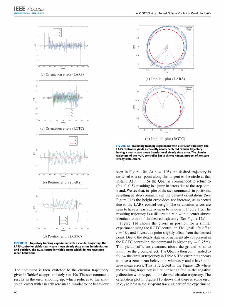
FIGURE 11. Trajectory tracking experiment with a circular trajectory. TheLARS controller yields nearly zero mean steady state errors in orientationand position. The RGTC controller yields errors which do not have zeromean behaviour.

The command is then switched to the circular trajecteorygiven in Table 6 at approximately t = 49s. The step commandresults in the error shooting up, which reduces to the sinu-soidal errors with a nearly zero mean, similar to the behaviour

−1−0.500.511.5

−1

−0.5

0

0.5

1

x [m]

y [

m]

trajectory

desired


−1−0.500.511.5

−1

−0.5

0

0.5

1

x [m]y [

m]

trajectory

desired


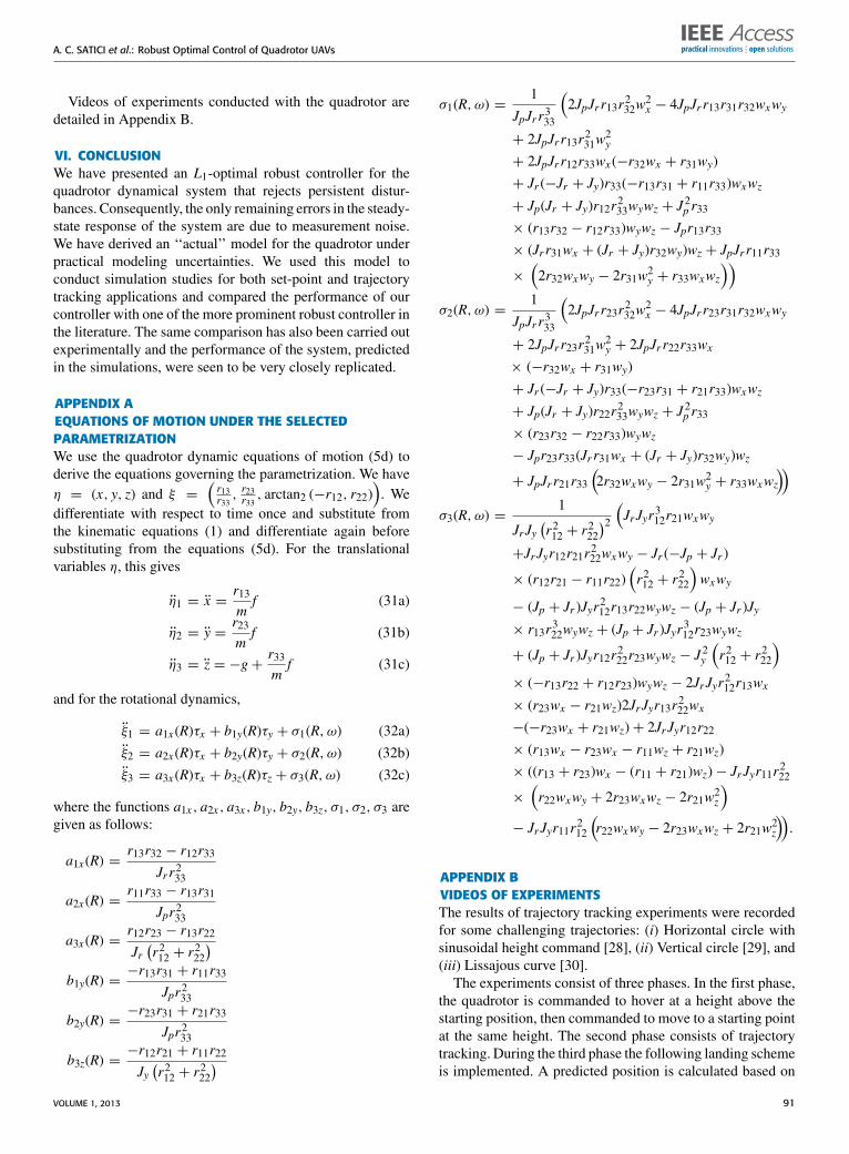
FIGURE 12. Trajectory tracking experiment with a circular trajectory. TheLARS controller yields a correctly nearly centered circular trajectory,having a nearly zero mean translational steady state error. The circulartrajectory of the RGTC controller has a shifted center, product of nonzerosteady state errors.

seen in Figure 10c. At t = 105s the desired trajectory isswitched to a set-point along the tangent to the circle at thatinstant. At t = 115s the Qball is commanded to return to(0.4, 0, 0.5), resulting in a jump in errors due to the step com-mand.We see that, in spite of the step commands in positions,resulting in step commands in the desired orientations (SeeFigure 11a) the height error does not increase, as expecteddue to the LARS control design. The orientation errors areseen to have a nearly zero mean behaviour in Figure 11a. Theresulting trajectory is a distorted circle with a center almostidentical to that of the desired trajectory (See Figure 12a).Figure 11d shows the errors in position for a similar

experiment using the RGTC controller. The Qball lifts off att = 18s, and hovers at a point slightly offset from the desiredpoint. Due to the steady state error in height always present inthe RGTC controller, the command is higher (zd = 0.75m).This yields sufficient clearance above the ground so as tominimize the ground effect. The Qball is then commanded tofollow the circular trajectory in Table 6. The error in x appearsto have a zero mean behaviour, whereas y and z have non-zero mean errors. This is reflected in the Figure 12b wherethe resulting trajectory is circular but shifted in the negativey direction with respect to the desired circular trajectory. Theorientation plot in Figure 11b shows that there is some errorin e23 at least in the set-point tracking part of the experiment.

90 VOLUME 1, 2013


Videos of experiments conducted with the quadrotor aredetailed in Appendix B.

VI. CONCLUSIONWe have presented an L1-optimal robust controller for thequadrotor dynamical system that rejects persistent distur-bances. Consequently, the only remaining errors in the steady-state response of the system are due to measurement noise.We have derived an ‘‘actual’’ model for the quadrotor underpractical modeling uncertainties. We used this model toconduct simulation studies for both set-point and trajectorytracking applications and compared the performance of ourcontroller with one of the more prominent robust controller inthe literature. The same comparison has also been carried outexperimentally and the performance of the system, predictedin the simulations, were seen to be very closely replicated.

APPENDIX AEQUATIONS OF MOTION UNDER THE SELECTEDPARAMETRIZATIONWe use the quadrotor dynamic equations of motion (5d) toderive the equations governing the parametrization. We haveη = (x, y, z) and ξ =

(r13r33,r23r33, arctan2 (−r12, r22)

). We

differentiate with respect to time once and substitute fromthe kinematic equations (1) and differentiate again beforesubstituting from the equations (5d). For the translationalvariables η, this gives

η1 = x =r13mf (31a)

η2 = y =r23mf (31b)

η3 = z = −g+r33mf (31c)

and for the rotational dynamics,

ξ1 = a1x(R)τx + b1y(R)τy + σ1(R, ω) (32a)

ξ2 = a2x(R)τx + b2y(R)τy + σ2(R, ω) (32b)

ξ3 = a3x(R)τx + b3z(R)τz + σ3(R, ω) (32c)

where the functions a1x , a2x , a3x , b1y, b2y, b3z, σ1, σ2, σ3 aregiven as follows:

a1x(R) =r13r32 − r12r33

Jrr233

a2x(R) =r11r33 − r13r31

Jpr233

a3x(R) =r12r23 − r13r22Jr(r212 + r

222

)b1y(R) =

−r13r31 + r11r33Jpr233

b2y(R) =−r23r31 + r21r33

Jpr233

b3z(R) =−r12r21 + r11r22Jy(r212 + r

222

)

σ1(R, ω) =1

JpJrr333

(2JpJrr13r232w

2x − 4JpJrr13r31r32wxwy

+ 2JpJrr13r231w2y

+ 2JpJrr12r33wx(−r32wx + r31wy)

+ Jr (−Jr + Jy)r33(−r13r31 + r11r33)wxwz+ Jp(Jr + Jy)r12r233wywz + J

2p r33

× (r13r32 − r12r33)wywz − Jpr13r33× (Jrr31wx + (Jr + Jy)r32wy)wz + JpJrr11r33

×

(2r32wxwy − 2r31w2

y + r33wxwz))

σ2(R, ω) =1

JpJrr333

(2JpJrr23r232w

2x − 4JpJrr23r31r32wxwy

+ 2JpJrr23r231w2y + 2JpJrr22r33wx

× (−r32wx + r31wy)

+ Jr (−Jr + Jy)r33(−r23r31 + r21r33)wxwz+ Jp(Jr + Jy)r22r233wywz + J

2p r33

× (r23r32 − r22r33)wywz− Jpr23r33(Jrr31wx + (Jr + Jy)r32wy)wz

+ JpJrr21r33(2r32wxwy − 2r31w2

y + r33wxwz))

σ3(R, ω) =1

JrJy(r212 + r

222

)2 (JrJyr312r21wxwy+JrJyr12r21r222wxwy − Jr (−Jp + Jr )

× (r12r21 − r11r22)(r212 + r

222

)wxwy

− (Jp + Jr )Jyr212r13r22wywz − (Jp + Jr )Jy× r13r322wywz + (Jp + Jr )Jyr312r23wywz

+ (Jp + Jr )Jyr12r222r23wywz − J2y

(r212 + r

222

)× (−r13r22 + r12r23)wywz − 2JrJyr212r13wx× (r23wx − r21wz)2JrJyr13r222wx−(−r23wx + r21wz)+ 2JrJyr12r22× (r13wx − r23wx − r11wz + r21wz)

× ((r13 + r23)wx − (r11 + r21)wz)− JrJyr11r222

×

(r22wxwy + 2r23wxwz − 2r21w2

z

)− JrJyr11r212

(r22wxwy − 2r23wxwz + 2r21w2

z

)).

APPENDIX BVIDEOS OF EXPERIMENTSThe results of trajectory tracking experiments were recordedfor some challenging trajectories: (i) Horizontal circle withsinusoidal height command [28], (ii) Vertical circle [29], and(iii) Lissajous curve [30].The experiments consist of three phases. In the first phase,

the quadrotor is commanded to hover at a height above thestarting position, then commanded to move to a starting pointat the same height. The second phase consists of trajectorytracking. During the third phase the following landing schemeis implemented. A predicted position is calculated based on

VOLUME 1, 2013 91


the quadrotor position and velocity at the end of the secondphase and commanded as a set-point. The desired height isdecreased in steps until the quadrotor can be powered downsafely.

The first trajectory is a horizontal circle with a vary-ing height command [28]. The varying height creates anincreased demand on quadrotor actuators. This is furthertested when the frequency of the height command is doubledduring the motion of the quadrotor.

The second experiment demonstrates the controller per-formance when gravity acts as a disturbance non-trivially.This is achieved by requiring the quadrotor to track a verticalcircle [29].

The third experiment shows the performance of the con-troller under a significantly aggressive motion: tracking athree dimensional Lissajous curve. The quadrotor motion isseen to be both stable and smooth throughout the experi-ment [30].

The reader is invited to view further videos on the UTDRobotics channel [31], not all of which use the L1−optimalcontroller. It can be observed that the tracking performance ispoorer and more sluggish when the quadrotor uses naive PIDcontrol.

REFERENCES[1] M. Spong, ‘‘Partial feedback linearization of underactuated mechanical

systems,’’ in Proc. IEEE/RSJ/GI Int. Conf. Intell. Robots Syst. Adv. Robot.Syst. Real World, vol. 1. Sep. 1994, pp. 314–321.

[2] P. Pounds, R. Mahony, P. Hynes, and J. Roberts, ‘‘Design of a four-rotor aerial robot,’’ in Proc. Australasian Conf. Robot. Autom., Nov. 2002,pp. 145–150.

[3] S. Bouabdallah, A. Noth, and R. Siegwart, ‘‘PID vs LQ control techniquesapplied to an indoor micro quadrotor,’’ in Proc. IEEE/RSJ Int. Conf. Intell.Robots Syst., vol. 3. Oct. 2004, pp. 2451–2456.

[4] R. Xu and U. Ozguner, ‘‘Sliding mode control of a quadrotor helicopter,’’in Proc. 45th IEEE Conf. Decision Control, Dec. 2006, pp. 4957–4962.

[5] S. Bouabdallah and R. Siegwart, ‘‘Backstepping and sliding-mode tech-niques applied to an indoor micro quadrotor,’’ in Proc. IEEE Int. Conf.Robot. Autom., Apr. 2005, pp. 2247–2252.

[6] T. Madani and A. Benallegue, ‘‘Backstepping control for a quadrotorhelicopter,’’ in Proc. IEEE/RSJ Int. Conf. Intell. Robots Syst., Oct. 2006,pp. 3255–3260.

[7] S. Bouabdallah, P. Murrieri, and R. Siegwart, ‘‘Design and control of anindoor micro quadrotor,’’ in Proc. IEEE Int. Conf. Robot. Autom., vol. 5.May 2004, pp. 4393–4398.

[8] T. Lee, M. Leoky, and N. McClamroch, ‘‘Geometric tracking control ofa quadrotor UAV on SE(3),’’ in Proc. 49th IEEE Conf. Decision Control,Dec. 2010, pp. 5420–5425.

[9] D. Mellinger and V. Kumar, ‘‘Minimum snap trajectory generation andcontrol for quadrotors,’’ in Proc. IEEE Int. Conf. Robot. Autom., May 2011,pp. 2520–2525.

[10] H. Khalil, Nonlinear Systems. Englewood Cliffs, NJ, USA:Prentice-Hall, 2002.

[11] V. Mistler, A. Benallegue, and N. M’Sirdi, ‘‘Exact linearization and nonin-teracting control of a 4 rotors helicopter via dynamic feedback,’’ in Proc.10th IEEE Int. Workshop Robot Human Interact. Commun., Jan. 2001,pp. 586–593.

[12] A. Mokhtari and A. Benallegue, ‘‘Dynamic feedback controller of eulerangles and wind parameters estimation for a quadrotor unmanned aerialvehicle,’’ in Proc. IEEE Int. Conf. Robot. Autom., vol. 3. May 2004,pp. 2359–2366.

[13] G. V. Raffo, M. G. Ortega, and F. R. Rubio, ‘‘An integral predic-tive/nonlinear control H∞ structure for a quadrotor helicopter,’’ Automat-ica, vol. 46, no. 1, pp. 29–39, Jan. 2010.

[14] A. Mokhtari, A. Benallegue, and B. Daachi, ‘‘Robust feedback lin-earization and GH∞ controller for a quadrotor unmanned aerial vehi-cle,’’ in Proc. IEEE/RSJ Int. Conf. Intell. Robots Syst., Aug. 2005,pp. 1198–1203.

[15] T. Lee, M. Leok, and N. H. McClamroch, ‘‘Nonlinear robust trackingcontrol of a quadrotor UAV on SE(3),’’ Asian J. Control, vol. 15, no. 2,pp. 391–408, Mar. 2013.

[16] C. Diao, B. Xian, Q. Yin, W. Zeng, H. Li, and Y. Yang, ‘‘A nonlinearadaptive control approach for quadrotor uavs,’’ in Proc. 8th Asian ControlConf. (ASCC), May 2011, pp. 223–228.

[17] T. Fernando, J. Chandiramani, T. Lee, and H. Gutierrez, ‘‘Robust adaptivegeometric tracking controls on SO(3) with an application to the attitudedynamics of a quadrotor uav,’’ in Proc. 50th IEEE Conf. Decision ControlEur. Control Conf., Dec. 2011, pp. 7380–7385.

[18] M. Spong and M. Vidyasagar, ‘‘Robust linear compensator design fornonlinear robotic control,’’ in Proc. IEEE Int. Conf. Robot. Autom., vol. 2.Mar. 1985, pp. 954–959.

[19] M. Spong and M. Vidyasagar, ‘‘Robust nonlinear control of robot manip-ulators,’’ in Proc. IEEE Conf. Decision Control, vol. 24. Dec. 1985,pp. 1767–1772.

[20] M. Spong and M. Vidyasagar, ‘‘Robust linear compensator designfor nonlinear robotic control,’’ IEEE J. Robot. Autom., vol. 3, no. 4,pp. 345–351, Aug. 1987.

[21] M. Vidyasagar, ‘‘Optimal rejection of persistent bounded disturbances,’’IEEE Trans. Autom. Control, vol. 31, no. 6, pp. 527–534, Jun. 1986.

[22] M. Vidyasagar, Control System Synthesis: A Factorization Approach (Syn-thesis Lectures on Control and Mechatronics). San Rafael, CA, USA:Morgan & Claypool Publishers, 2011.

[23] Quanser Inc. (2013, Apr.). Quanser Qball-X4, Markham,Canada [Online]. Available: http://www.quanser.com/english/html/UVS_Lab/fs_Qball_X4.htm

[24] J. Marsden and T. Ratiu, Introduction to Mechanics and Symmetry: A BasicExposition of Classical Mechanical Systems (Texts in Applied Mathemat-ics). New York, NY, USA: Springer-Verlag, 1999.

[25] C. Nett, C. Jacobson, andM. Balas, ‘‘A connection between state-space anddoubly coprime fractional representations,’’ IEEE Trans. Autom. Control,vol. 29, no. 9, pp. 831–832, Sep. 1984.

[26] Vicon Motion Systems Ltd. (2012). Vicon MX Giganet GigabitEthernet Controller, Oxford, U.K. [Online]. Available: http://www.vicon.com/products/mxgiganet.html

[27] E. Kreyszig, Differential Geometry (Dover books on advanced mathemat-ics). New York, NY, USA: Dover, 1991.

[28] Laboratory for Autonomous Robotics, UT Dallas. (2012). QuadrotorTracking a Horizontal Circle with Sinusoidal Height Command,Cambridge, MA, USA [Online]. Available: http://www.youtube.com/watch?v=xZwQ3Uis4dc

[29] Laboratory for Autonomous Robotics, UT Dallas. (2012). QuadrotorTracking a Vertical Circle, Cambridge, MA, USA [Online]. Available:http://www.youtube.com/watch?v=TqY4TcJXEcY

[30] Laboratory for Autonomous Robotics, UT Dallas. (2012). QuadrotorTracking a Lissajous Curve, Cambridge, MA, USA [Online]. Available:http://www.youtube.com/watch?v=1lIGlwu3Cic

[31] Laboratory for Autonomous Robotics, UT Dallas. (2012). UTD RoboticsChannel on Youtube, Cambridge, MA, USA [Online]. Available:http://www.youtube.com/UTDRobotics

AYKUT C. SATICI received the B.Sc. and M.Sc.degrees in mechatronics engineering from SabanciUniversity, Istanbul, Turkey, in 2008 and 2010,respectively, and the Masters degree in mathemat-ics from the University of Texas, Dallas, TX, USA,in 2013. He is currently with the Electrical Engi-neering Department, University of Texas at Dal-las. His current research interests include robotics,geometric mechanics, and cooperative control.

92 VOLUME 1, 2013


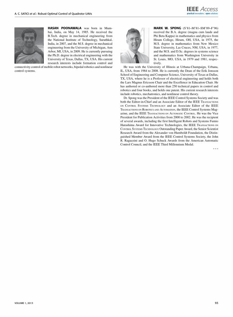
HASAN POONAWALA was born in Mum-bai, India, on May 14, 1985. He received theB.Tech. degree in mechanical engineering fromthe National Institute of Technology, Surathkal,India, in 2007, and the M.S. degree in mechanicalengineering from the University of Michigan, AnnArbor, MI, USA, in 2009. He is currently pursuingthe Ph.D. degree in electrical engineering with theUniversity of Texas, Dallas, TX, USA. His currentresearch interests include formation control and

connectivity control of mobile robot networks, bipedal robotics and nonlinearcontrol systems.

MARK W. SPONG (S’81–M’81–SM’89–F’96)received the B.A. degree (magna cum laude andPhi Beta Kappa) in mathematics and physics fromHiram College, Hiram, OH, USA, in 1975, theM.S. degree in mathematics from New MexicoState University, Las Cruces, NM, USA, in 1977,and the M.S. and D.Sc. degrees in systems scienceand mathematics from Washington University inSt. Louis, MO, USA, in 1979 and 1981, respec-tively.

He was with the University of Illinois at Urbana-Champaign, Urbana,IL, USA, from 1984 to 2008. He is currently the Dean of the Erik JonssonSchool of Engineering and Computer Science, University of Texas at Dallas,TX, USA, where he is a Professor of electrical engineering and holds boththe Lars Magnus Ericsson Chair and the Excellence in Education Chair. Hehas authored or co-authored more than 250 technical papers in control androbotics and four books, and holds one patent. His current research interestsinclude robotics, mechatronics, and nonlinear control theory.

Dr. Spong was the President of the IEEE Control Systems Society and wasboth the Editor-in-Chief and an Associate Editor of the IEEE TRANSACTIONS

ON CONTROL SYSTEMS TECHNOLOGY and an Associate Editor of the IEEETRANSACTIONS ON ROBOTICS AND AUTOMATION, the IEEE Control Systems Mag-azine, and the IEEE TRANSACTIONS ON AUTOMATIC CONTROL. He was the VicePresident for Publication Activities from 2000 to 2002. He was the recipientof several awards, including the first Intelligent Robots and Systems FumioHarashima Award for Innovative Technologies, the IEEE TRANSACTIONS ON

CONTROL SYSTEMSTECHNOLOGYOutstanding Paper Award, the Senior ScientistResearch Award from the Alexander von Humboldt Foundation, the Distin-guished Member Award from the IEEE Control Systems Society, the JohnR. Ragazzini and O. Hugo Schuck Awards from the American AutomaticControl Council, and the IEEE Third Millennium Medal.

VOLUME 1, 2013 93

Documents

Robust Optimal Control of Quadrotor UAVs