Simulating Low Frequency Reverberation in Rooms

IN DEGREE PROJECT MECHANICAL ENGINEERING,SECOND CYCLE, 30 CREDITS

, STOCKHOLM SWEDEN 2020

Simulating Low Frequency Reverberation in Rooms

MATTIAS SVENSSON

KTH ROYAL INSTITUTE OF TECHNOLOGYSCHOOL OF ENGINEERING SCIENCES

2

3

Simulating Low Frequency Reverberation in Rooms

Mattias Svensson

2020-06-07

TRITA-AVE ISSN

KTH Royal Institute of Technology School of Engineering Sciences Department of Aeronautical and Vehicle Engineering SE-100 44 Stockholm, Sweden Examiner: Hans Bodén, KTH Royal Institute of Technology Supervision: Peter Blom, ACAD International AB

4

i

Abstract The aim of this thesis was to make a practical tool for low frequency analysis in room acous-tics. The need arises from Acad’s experience that their results from simulations using ray-tracing software deviate in the lower frequencies when compared to field measurements in rooms. The tool was programmed in Matlab and utilizes the Finite Difference Time Domain (FDTD) method, which is a form of rapid finite element analysis in the time domain.

A number of tests have been made to investigate the practical limitations of the FDTD method, such as numerical errors caused by sound sources, discretization and simulation time. Boundary conditions, with and without frequency dependence, have been analysed by comparing results from simulations of a virtual impedance tube and reverberation room to analytical solutions. These tests show that the use of the FDTD method appears well suited for the purpose of the tool.

A field test was made to verify that the tool enables easy and relatively quick simulations of real rooms, with results well in line with measured acoustic parameters. Comparisons of the results from using the FDTD method, ray-tracing and finite elements (FEM) showed good correlation. This indicates that the deviations Acad experience between simulated results and field measurements are most likely caused by uncertainties in the sound absorption data used for low frequencies rather than by limitations in the ray-tracing software. The FDTD tool might still come in handy for more complex models, where edge diffraction is a more important factor, or simply as a means for a “second opinion” to ray-tracing - in general FEM is too time consuming a method to be used on a daily basis.

Auxiliary tools made for importing models, providing output data in the of room acoustic parameters, graphs and audio files are not covered in detail here, as these lay outside the scope of this thesis.

Keywords: Low frequencies, Room acoustics, Finite Difference Time Domain method, FDTD.

ii

iii

Sammanfattning Målet för detta examensarbete var att undersöka möjligheten att programmera ett praktiskt användbart verktyg för lågfrekvensanalys inom rumsakustik. Behovet uppstår från Acads erfarenhet att resultat från simuleringar med hjälp av strålgångsmjukvara avviker i lågfre-kvensområdet i jämförelse med fältmätningar i färdigställda rum. Verktyget är programme-rat i Matlab och använder Finite Difference Time Domain (FDTD) metoden, vilket är en typ av snabb finita elementanalys i tidsdomänen.

En rad tester har genomförts för att se metodens praktiska begräsningar orsakade av nume-riska fel vid val av ljudkälla, diskretisering och simuleringstid. Randvillkor, med och utan frekvensberoende, har analyserats genom jämförelser av simulerade resultat i virtuella im-pedansrör och efterklangsrum mot analytiska beräkningar. Testerna visar att FDTD-meto-den tycks fungerar väl för verktygets tilltänkta användningsområde.

Ett fälttest genomfördes för att verifiera att det med verktyget är möjligt att enkelt och rela-tivt snabbt simulera resultat som väl matcher uppmätta rumsakustiska parametrar. Jämfö-relser mellan FDTD-metoden och resultat beräknade med strålgångsanalys och finita ele-mentmetoden (FEM) visade även på god korrelation. Detta indikerar att de avvikelser Acad erfar mellan simulerade resultat och fältmätningar troligen orsakas av osäkerheter i den in-gående ljudabsorptionsdata som används för låga frekvenser, snarare än av begränsningar i strålgångsmjukvaran. Verktyget kan fortfarande komma till användning för mer komplexa modeller, där kantdiffraktion är en viktigare faktor, eller helt enkelt som ett sätt att få ett ”andra utlåtande” till resultaten från strålgångsmjukvaran då FEM-analys generellt är en för tidskrävande metod för att användas på daglig basis.

Kringverktyg skapade för t.ex. import av modeller, utdata i form av rumsakustiska paramet-rar, grafer och ljudfiler redovisas inte i detalj i denna rapport eftersom dessa ligger utanför examensarbetet.

Nyckelord:

Rumsakustik, låga frekvenser, Finite Difference Time Domain metoden, FDTD.

iv

Contents Notations ................................................................................................................................. 1

1. Introduction .................................................................................................................... 2

2. Introduction to the Finite Difference Time Domain method ......................................... 3

2.1. Governing equations ................................................................................................ 3

2.2. Discretization ........................................................................................................... 5

2.2.1. Non-staggered example in 1-D ......................................................................... 5

2.2.2. Staggered time scheme example in 1-D ............................................................ 8

2.2.3. Staggered spatial grid and time scheme example in 1-D ................................ 10

2.2.4. The FDTD method in 2-D and 3-D .................................................................. 11

2.3. Stability and the choice of temporal step and element size ................................... 14

2.3.1. Spatial step/element size ................................................................................ 14

2.3.2. Temporal step size .......................................................................................... 15

2.4. Schemes of higher order ........................................................................................ 16

2.4.1. Sound source(s) .............................................................................................. 17

2.4.2. Numerical errors ............................................................................................. 21

3. Boundary conditions ..................................................................................................... 26

3.1. 1-DOF mass, spring and damper boundary condition ........................................... 27

4. Validations .................................................................................................................... 31

4.1. 1-DOF BC at normal incidence ............................................................................... 31

4.2. 1-DOF BC at random incidence.............................................................................. 36

4.3. Directivity of the Botteldooren boundary condition .............................................. 42

4.4. PML and Botteldooren’s boundary condition ........................................................ 44

5. Modelling ...................................................................................................................... 47

6. Simulation of a classroom .............................................................................................48

6.1. Field measurements ...............................................................................................48

6.2. Modelling and importing to Matlab .......................................................................48

6.3. Material parameters ............................................................................................... 50

6.4. Spatial step size and convergation ......................................................................... 50

6.5. Comparison to field measurement results ............................................................. 51

6.6. Comparison to FEM and ray-tracing software ...................................................... 52

7. Concluding remarks .......................................................................................................... 53

7. References ..................................................................................................................... 55

Appendix A ............................................................................................................................ 57

Appendix B ............................................................................................................................ 58

1

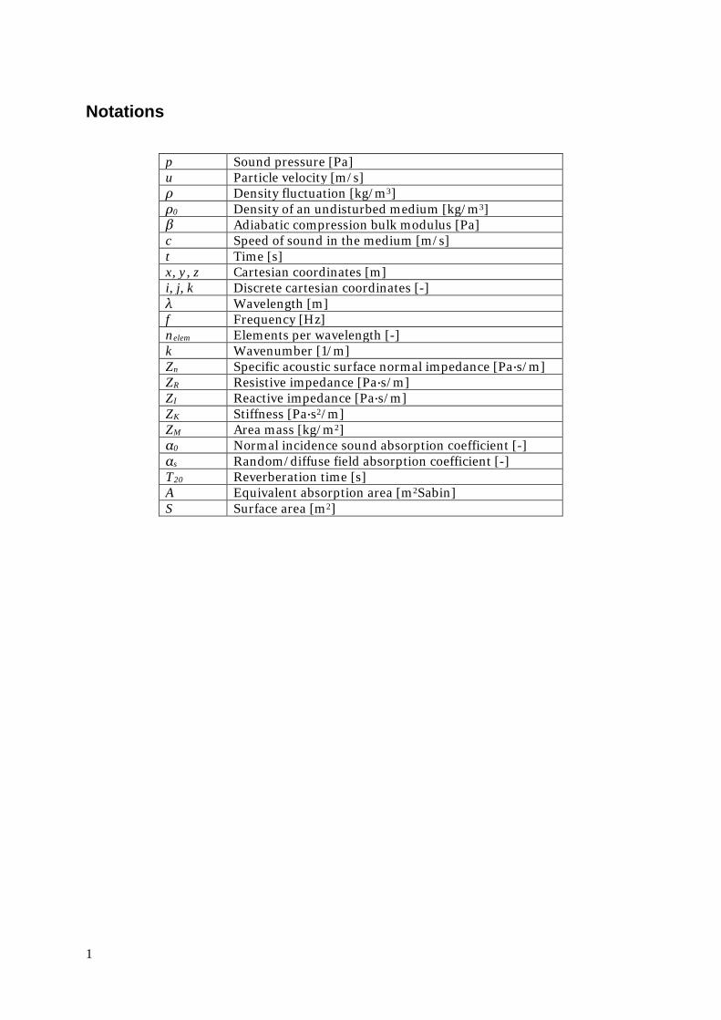
Notations

p Sound pressure [Pa] u Particle velocity [m/s] ρ Density fluctuation [kg/m3] ρ0 Density of an undisturbed medium [kg/m3] β Adiabatic compression bulk modulus [Pa] c Speed of sound in the medium [m/s] t Time [s] x, y, z Cartesian coordinates [m] i, j, k Discrete cartesian coordinates [-] λ Wavelength [m] f Frequency [Hz] nelem Elements per wavelength [-] k Wavenumber [1/m] Zn Specific acoustic surface normal impedance [Pa∙s/m] ZR Resistive impedance [Pa∙s/m] ZI Reactive impedance [Pa∙s/m] ZK Stiffness [Pa∙s2/m] ZM Area mass [kg/m2] α0 Normal incidence sound absorption coefficient [-] αs Random/diffuse field absorption coefficient [-] T20 Reverberation time [s] A Equivalent absorption area [m2Sabin] S Surface area [m2]

2

1. Introduction The ability to correctly predict the acoustics of a room and plan the acoustic treatment right from the start can save a lot of money, time and environmental impact. In Acad’s experience, results from predicted reverberation time from ray-tracing simulations usually match field measurements in the finished room at high frequencies, from the octave band 250 Hz and higher. However, at lower frequencies the measured results usually deviate from the pre-dicted ones. As the reverberation time in the 125 Hz octave band is important for speech intelligibility, a mean to better simulate low frequency behaviour is desired.

Ray-tracing simulations utilizes sound energy, not taking into account the phase infor-mation of the sound “rays”. While this provides good approximations at higher frequencies, especially where the sound field can be considered diffuse, the approach falls short in pre-dicting low frequency phenomena such as standing waves, phase cancellation and diffrac-tion. Commercial FEM software, such as Ansys, is well suited for these calculations, but be-comes unpractically complex in the role of a simple complement to a ray-tracing software FEM as new models must be made and meshed.

The aim of this thesis was to investigate the possibility of making a simple tool to extend the low frequency limit of room acoustics analysis made in ray-tracing software, such as Odeon, utilizing the same 3D-model and material selections.

The Finite Difference Time Domain (FDTD) method was chosen based on its simplicity and its promising ability to simulate low frequency phenomena.

3

2. Introduction to the Finite Difference Time Domain method The Finite Difference Time Domain (FDTD) method is a well-known numerical analysis tech-nique, originally developed for simulating electromagnetic propagation. Formulated by Kane Yee (hence sometimes referred to as the Yee method) in 1966 to solve the Maxwell’s curl equa-tions [1], it has since been adapted for use in optics and acoustics. In its basic form, the method is a finite-difference approximation of both space and time derivatives of the governing equa-tions, using leapfrog scheme in time on staggered Cartesian grids in space for each discrete field component. The groundwork for acoustical applications by the FDTD method was laid by Botteldooren in the paper “Acoustical finite-difference time-domain simulation in a quasi-Car-tesian grid” in 1993 [2].

The strengths of the FDTD method are, for example:

• Numerically simple and easy to understand. • Uses the time domain, thus suitable for auralization and study of transients. • A single prediction can cover a wide range of frequencies. • Capable of simulating low frequency phenomena, like diffraction and phase cancella-

tion. • Capable of simulating time variant systems. • Simple ideally rigid or purely absorbing boundaries are easily implemented.

The challenges of the FDTD method are, for example:

• Requires large numbers of elements/meshes for simulating high frequencies. • Complex boundary conditions are hard to implement, especially if the they are fre-

quency varying (as real boundaries often are).

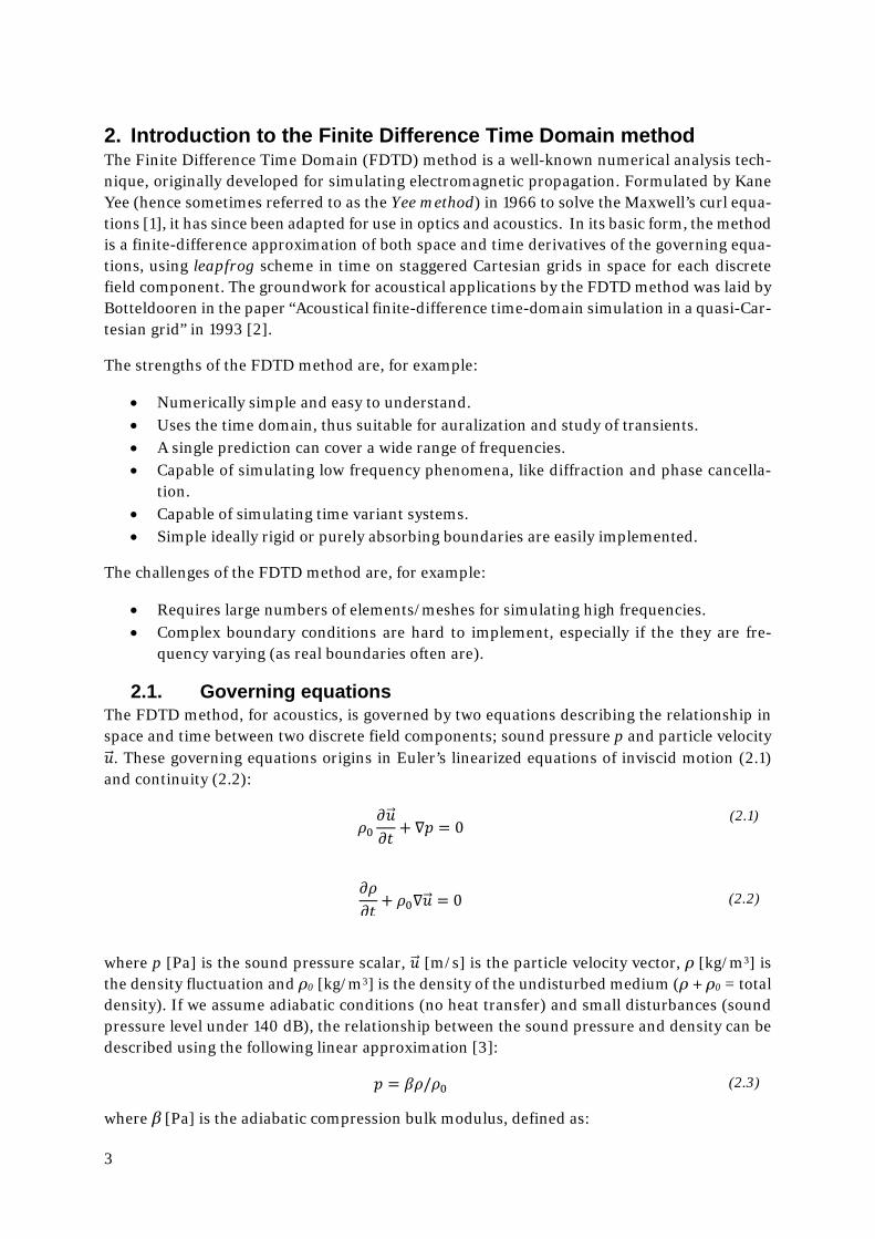
2.1. Governing equations The FDTD method, for acoustics, is governed by two equations describing the relationship in space and time between two discrete field components; sound pressure p and particle velocity 𝑢𝑢�⃗ . These governing equations origins in Euler’s linearized equations of inviscid motion (2.1) and continuity (2.2):

𝜌𝜌0𝜕𝜕𝑢𝑢�⃗𝜕𝜕𝜕𝜕

+ ∇𝑝𝑝 = 0 (2.1)

𝜕𝜕𝜌𝜌𝜕𝜕𝜕𝜕

+ 𝜌𝜌0∇𝑢𝑢�⃗ = 0 (2.2)

where p [Pa] is the sound pressure scalar, 𝑢𝑢�⃗ [m/s] is the particle velocity vector, ρ [kg/m3] is the density fluctuation and ρ0 [kg/m3] is the density of the undisturbed medium (ρ + ρ0 = total density). If we assume adiabatic conditions (no heat transfer) and small disturbances (sound pressure level under 140 dB), the relationship between the sound pressure and density can be described using the following linear approximation [3]:

𝑝𝑝 = 𝛽𝛽𝜌𝜌/𝜌𝜌0 (2.3)

where β [Pa] is the adiabatic compression bulk modulus, defined as:

4

(𝛽𝛽 = 𝑐𝑐2𝜌𝜌0) (2.4)

where c [m/s] is the speed of sound in the medium. Inserting (2.3) into (2.2) yields:

𝜕𝜕𝑝𝑝𝜕𝜕𝜕𝜕

+ 𝛽𝛽∇𝑢𝑢�⃗ = 0 (2.5)

This leaves us with two governing equations for the FDTD method, describing the relationship between the first order time derivative of the particle velocity and the first order spatial deriv-ative of the sound pressure (2.6), and vice versa (2.7):

𝜕𝜕𝑢𝑢�⃗𝜕𝜕𝜕𝜕

= −1𝜌𝜌0∇𝑝𝑝 (2.6)

𝜕𝜕𝑝𝑝𝜕𝜕𝜕𝜕

= −𝛽𝛽∇𝑢𝑢�⃗ (2.7)

Breaking out the velocity vector components (ux, uy and uz) from 𝑢𝑢�⃗ and adding notation for time (n∙∆t [s]) and space in 3-D Cartesian coordinates (i∙∆x, j∙∆y, k∙∆z [m]), equation (2.6) and (2.7) will read:

𝜕𝜕𝜕𝜕𝜕𝜕𝑢𝑢𝑥𝑥𝑛𝑛(𝑖𝑖, 𝑗𝑗,𝑘𝑘) = −

1𝜌𝜌0

𝜕𝜕𝜕𝜕𝜕𝜕

𝑝𝑝𝑛𝑛(𝑖𝑖, 𝑗𝑗,𝑘𝑘) (2.8)

𝜕𝜕𝜕𝜕𝜕𝜕𝑢𝑢𝑦𝑦𝑛𝑛(𝑖𝑖, 𝑗𝑗,𝑘𝑘) = −

1𝜌𝜌0

𝜕𝜕𝜕𝜕𝜕𝜕

𝑝𝑝𝑛𝑛(𝑖𝑖, 𝑗𝑗,𝑘𝑘) (2.9)

𝜕𝜕𝜕𝜕𝜕𝜕𝑢𝑢𝑧𝑧𝑛𝑛(𝑖𝑖, 𝑗𝑗,𝑘𝑘) = −

1𝜌𝜌0

𝜕𝜕𝜕𝜕𝜕𝜕𝑝𝑝𝑛𝑛(𝑖𝑖, 𝑗𝑗,𝑘𝑘) (2.10)

𝜕𝜕𝜕𝜕𝜕𝜕𝑝𝑝𝑛𝑛(𝑖𝑖, 𝑗𝑗,𝑘𝑘) = −𝛽𝛽�

𝜕𝜕𝜕𝜕𝜕𝜕

𝑢𝑢𝑥𝑥𝑛𝑛(𝑖𝑖, 𝑗𝑗, 𝑘𝑘) +𝜕𝜕𝜕𝜕𝜕𝜕

𝑢𝑢𝑦𝑦𝑛𝑛(𝑖𝑖, 𝑗𝑗,𝑘𝑘) +𝜕𝜕𝜕𝜕𝜕𝜕𝑢𝑢𝑧𝑧𝑛𝑛(𝑖𝑖, 𝑗𝑗, 𝑘𝑘)� (2.11)

5

2.2. Discretization The discretization in space (meshing) can be performed in the same manner as in any finite element method by dividing the domain into elements of appropriate shapes and sizes. In the FDTD method as formulated by Yee, the domain is discretized using a structured grid, using quadrilateral elements in 2-D and hexahedron (cubic) elements in 3-D.

In addition to the spatial discretization, the FDTD method also requires discretization in time to simulate transient systems by discrete time stepping.

Yee’s FDTD method uses a staggered grid for the spatial and temporal discretization. The first order derivatives of the governing equations are discretized by central difference approxima-tion of second order accuracy. This choice (and implementation) of a staggered discretization can be a bit hard to follow at a first glance, so a good approach for explaining this might be to start with a simple discretization of a 1-D model using a non-staggered grid (readers familiar with FD operators and their order of accuracy might want to jump ahead to 2.2.4 The FDTD method in 2-D and 3-D):

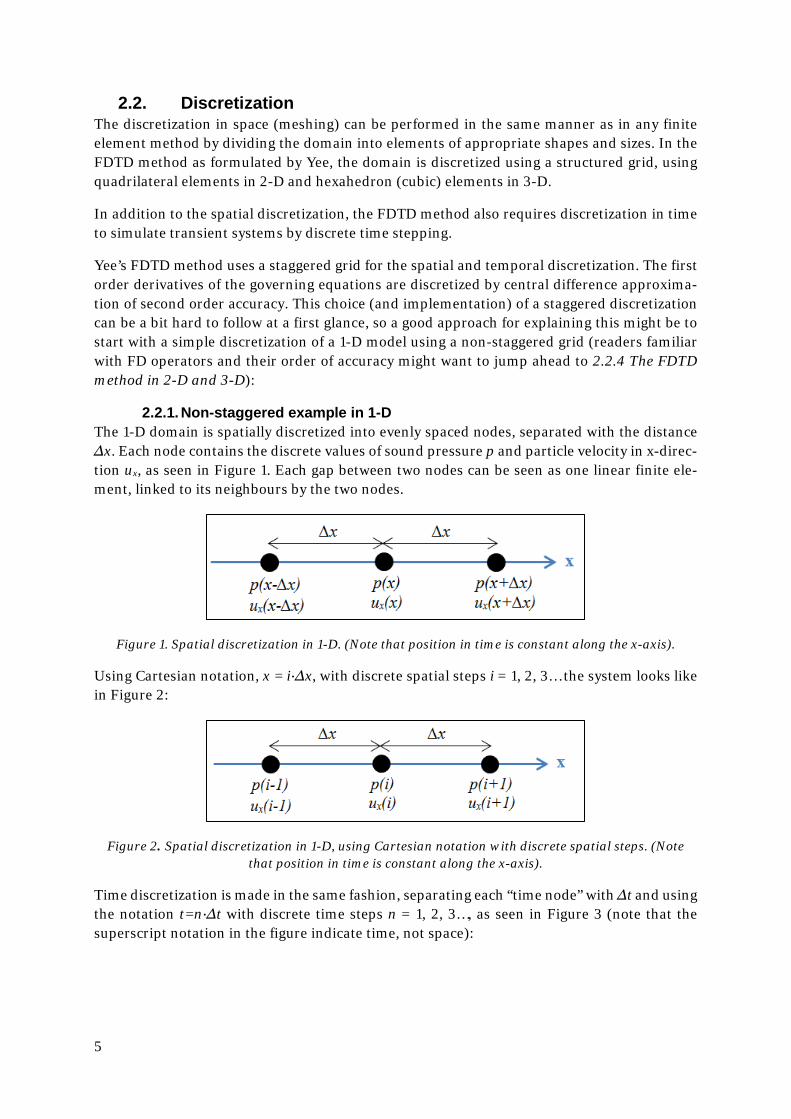
2.2.1. Non-staggered example in 1-D The 1-D domain is spatially discretized into evenly spaced nodes, separated with the distance ∆x. Each node contains the discrete values of sound pressure p and particle velocity in x-direc-tion ux, as seen in Figure 1. Each gap between two nodes can be seen as one linear finite ele-ment, linked to its neighbours by the two nodes.

Figure 1. Spatial discretization in 1-D. (Note that position in time is constant along the x-axis).

Using Cartesian notation, x = i∙∆x, with discrete spatial steps i = 1, 2, 3… the system looks like in Figure 2:

Figure 2. Spatial discretization in 1-D, using Cartesian notation with discrete spatial steps. (Note that position in time is constant along the x-axis).

Time discretization is made in the same fashion, separating each “time node” with ∆t and using the notation t=n∙∆t with discrete time steps n = 1, 2, 3…, as seen in Figure 3 (note that the superscript notation in the figure indicate time, not space):

6

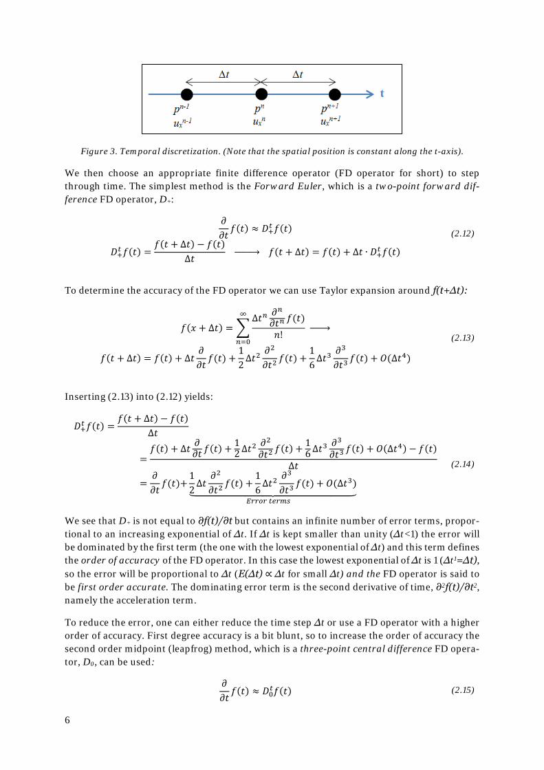
Figure 3. Temporal discretization. (Note that the spatial position is constant along the t-axis).

We then choose an appropriate finite difference operator (FD operator for short) to step through time. The simplest method is the Forward Euler, which is a two-point forward dif-ference FD operator, D+:

𝜕𝜕𝜕𝜕𝜕𝜕𝑓𝑓(𝜕𝜕) ≈ 𝐷𝐷+𝑡𝑡 𝑓𝑓(𝜕𝜕)

𝐷𝐷+𝑡𝑡 𝑓𝑓(𝜕𝜕) =𝑓𝑓(𝜕𝜕 + ∆𝜕𝜕) − 𝑓𝑓(𝜕𝜕)

∆𝜕𝜕

�⎯⎯⎯⎯� 𝑓𝑓(𝜕𝜕 + ∆𝜕𝜕) = 𝑓𝑓(𝜕𝜕) + ∆𝜕𝜕 ∙ 𝐷𝐷+𝑡𝑡 𝑓𝑓(𝜕𝜕)

(2.12)

To determine the accuracy of the FD operator we can use Taylor expansion around f(t+∆t):

𝑓𝑓(𝜕𝜕 + ∆𝜕𝜕) = �∆𝜕𝜕𝑛𝑛 𝜕𝜕

𝑛𝑛

𝜕𝜕𝜕𝜕𝑛𝑛 𝑓𝑓(𝜕𝜕)𝑛𝑛!

∞

𝑛𝑛=0

�⎯⎯�

𝑓𝑓(𝜕𝜕 + ∆𝜕𝜕) = 𝑓𝑓(𝜕𝜕) + ∆𝜕𝜕𝜕𝜕𝜕𝜕𝜕𝜕𝑓𝑓(𝜕𝜕) +

12∆𝜕𝜕2

𝜕𝜕2

𝜕𝜕𝜕𝜕2𝑓𝑓(𝜕𝜕) +

16∆𝜕𝜕3

𝜕𝜕3

𝜕𝜕𝜕𝜕3𝑓𝑓(𝜕𝜕) + 𝑂𝑂(∆𝜕𝜕4)

(2.13)

Inserting (2.13) into (2.12) yields:

𝐷𝐷+𝑡𝑡 𝑓𝑓(𝜕𝜕) =𝑓𝑓(𝜕𝜕 + ∆𝜕𝜕) − 𝑓𝑓(𝜕𝜕)

∆𝜕𝜕

=𝑓𝑓(𝜕𝜕) + ∆𝜕𝜕 𝜕𝜕𝜕𝜕𝜕𝜕 𝑓𝑓(𝜕𝜕) + 1

2∆𝜕𝜕2 𝜕𝜕2𝜕𝜕𝜕𝜕2 𝑓𝑓(𝜕𝜕) + 1

6∆𝜕𝜕3 𝜕𝜕3𝜕𝜕𝜕𝜕3 𝑓𝑓(𝜕𝜕) + 𝑂𝑂(∆𝜕𝜕4) − 𝑓𝑓(𝜕𝜕)

∆𝜕𝜕

=𝜕𝜕𝜕𝜕𝜕𝜕𝑓𝑓(𝜕𝜕)+

12∆𝜕𝜕

𝜕𝜕2

𝜕𝜕𝜕𝜕2𝑓𝑓(𝜕𝜕) +

16∆𝜕𝜕2

𝜕𝜕3

𝜕𝜕𝜕𝜕3𝑓𝑓(𝜕𝜕) + 𝑂𝑂(∆𝜕𝜕3)��

𝐸𝐸𝐸𝐸𝐸𝐸𝐸𝐸𝐸𝐸 𝑡𝑡𝑡𝑡𝐸𝐸𝑡𝑡𝑡𝑡

(2.14)

We see that D+ is not equal to ∂f(t)/∂t but contains an infinite number of error terms, propor-tional to an increasing exponential of ∆t. If ∆t is kept smaller than unity (∆t<1) the error will be dominated by the first term (the one with the lowest exponential of ∆t) and this term defines the order of accuracy of the FD operator. In this case the lowest exponential of ∆t is 1 (∆t1=∆t), so the error will be proportional to ∆t (E(∆t) ∝ ∆t for small ∆t) and the FD operator is said to be first order accurate. The dominating error term is the second derivative of time, ∂2f(t)/∂t2, namely the acceleration term.

To reduce the error, one can either reduce the time step ∆t or use a FD operator with a higher order of accuracy. First degree accuracy is a bit blunt, so to increase the order of accuracy the second order midpoint (leapfrog) method, which is a three-point central difference FD opera-tor, D0, can be used:

𝜕𝜕𝜕𝜕𝜕𝜕𝑓𝑓(𝜕𝜕) ≈ 𝐷𝐷0𝑡𝑡𝑓𝑓(𝜕𝜕) (2.15)

7

𝐷𝐷0𝑡𝑡𝑓𝑓(𝜕𝜕) =𝑓𝑓(𝜕𝜕 + ∆𝜕𝜕) − 𝑓𝑓(𝜕𝜕 − ∆𝜕𝜕)

2∆𝜕𝜕

�⎯⎯⎯⎯� 𝑓𝑓(𝜕𝜕 + ∆𝜕𝜕) = 𝑓𝑓(𝜕𝜕 − ∆𝜕𝜕) + 2∆𝜕𝜕 ∙ 𝐷𝐷0𝑡𝑡𝑓𝑓(𝜕𝜕)

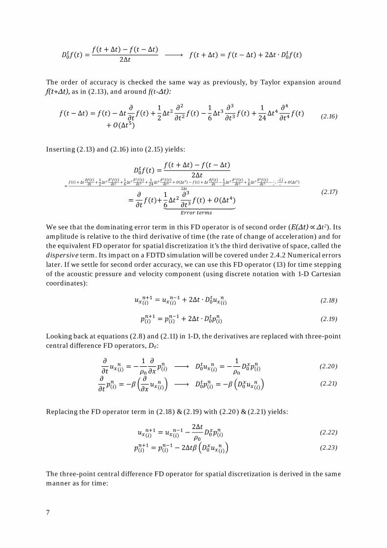
The order of accuracy is checked the same way as previously, by Taylor expansion around f(t+∆t), as in (2.13), and around f(t-∆t):

𝑓𝑓(𝜕𝜕 − ∆𝜕𝜕) = 𝑓𝑓(𝜕𝜕) − ∆𝜕𝜕𝜕𝜕𝜕𝜕𝜕𝜕𝑓𝑓(𝜕𝜕) +

12∆𝜕𝜕2

𝜕𝜕2

𝜕𝜕𝜕𝜕2𝑓𝑓(𝜕𝜕) −

16∆𝜕𝜕3

𝜕𝜕3

𝜕𝜕𝜕𝜕3𝑓𝑓(𝜕𝜕) +

124

∆𝜕𝜕4𝜕𝜕4

𝜕𝜕𝜕𝜕4𝑓𝑓(𝜕𝜕)

+ 𝑂𝑂(∆𝜕𝜕5) (2.16)

Inserting (2.13) and (2.16) into (2.15) yields:

𝐷𝐷0𝑡𝑡𝑓𝑓(𝜕𝜕) =𝑓𝑓(𝜕𝜕 + ∆𝜕𝜕) − 𝑓𝑓(𝜕𝜕 − ∆𝜕𝜕)

2∆𝜕𝜕

=𝑓𝑓(𝜕𝜕) + ∆𝜕𝜕 𝜕𝜕𝑓𝑓(𝜕𝜕)

𝜕𝜕𝜕𝜕 + 12∆𝜕𝜕

2 𝜕𝜕2𝑓𝑓(𝜕𝜕)𝜕𝜕𝜕𝜕2 + 1

6∆𝜕𝜕3 𝜕𝜕3𝑓𝑓(𝜕𝜕)

𝜕𝜕𝜕𝜕3 + 124∆𝜕𝜕

4 𝜕𝜕4𝑓𝑓(𝜕𝜕)𝜕𝜕𝜕𝜕4 + 𝑂𝑂(∆𝜕𝜕5)− 𝑓𝑓(𝜕𝜕) + ∆𝜕𝜕 𝜕𝜕𝑓𝑓(𝜕𝜕)

𝜕𝜕𝜕𝜕 − 12∆𝜕𝜕

2 𝜕𝜕2𝑓𝑓(𝜕𝜕)𝜕𝜕𝜕𝜕2 + 1

6∆𝜕𝜕3 𝜕𝜕3𝑓𝑓(𝜕𝜕)

𝜕𝜕𝜕𝜕3 − 1

24∆𝜕𝜕

4𝜕𝜕

4

𝑓𝑓(𝜕𝜕)𝜕𝜕𝜕𝜕

4+ 𝑂𝑂(∆𝜕𝜕5)

2∆𝜕𝜕

=𝜕𝜕𝜕𝜕𝜕𝜕𝑓𝑓(𝜕𝜕)+

16∆𝜕𝜕2

𝜕𝜕3

𝜕𝜕𝜕𝜕3𝑓𝑓(𝜕𝜕) + 𝑂𝑂(∆𝜕𝜕4)��

𝐸𝐸𝐸𝐸𝐸𝐸𝐸𝐸𝐸𝐸 𝑡𝑡𝑡𝑡𝐸𝐸𝑡𝑡𝑡𝑡

(2.17)

We see that the dominating error term in this FD operator is of second order (E(∆t) ∝ ∆t2). Its amplitude is relative to the third derivative of time (the rate of change of acceleration) and for the equivalent FD operator for spatial discretization it’s the third derivative of space, called the dispersive term. Its impact on a FDTD simulation will be covered under 2.4.2 Numerical errors later. If we settle for second order accuracy, we can use this FD operator (13) for time stepping of the acoustic pressure and velocity component (using discrete notation with 1-D Cartesian coordinates):

𝑢𝑢𝑥𝑥(𝑖𝑖)𝑛𝑛+1 = 𝑢𝑢𝑥𝑥(𝑖𝑖)

𝑛𝑛−1 + 2∆𝜕𝜕 ∙ 𝐷𝐷0𝑡𝑡𝑢𝑢𝑥𝑥(𝑖𝑖)𝑛𝑛 (2.18)

𝑝𝑝(𝑖𝑖)𝑛𝑛+1 = 𝑝𝑝(𝑖𝑖)

𝑛𝑛−1 + 2∆𝜕𝜕 ∙ 𝐷𝐷0𝑡𝑡𝑝𝑝(𝑖𝑖)𝑛𝑛 (2.19)

Looking back at equations (2.8) and (2.11) in 1-D, the derivatives are replaced with three-point central difference FD operators, D0:

𝜕𝜕𝜕𝜕𝜕𝜕𝑢𝑢𝑥𝑥(𝑖𝑖)

𝑛𝑛 = −1𝜌𝜌0

𝜕𝜕𝜕𝜕𝜕𝜕

𝑝𝑝(𝑖𝑖)𝑛𝑛

�⎯⎯� 𝐷𝐷0𝑡𝑡𝑢𝑢𝑥𝑥(𝑖𝑖)

𝑛𝑛 = −1𝜌𝜌0𝐷𝐷0𝑥𝑥𝑝𝑝(𝑖𝑖)

𝑛𝑛 (2.20)

𝜕𝜕𝜕𝜕𝜕𝜕𝑝𝑝(𝑖𝑖)𝑛𝑛 = −𝛽𝛽 �

𝜕𝜕𝜕𝜕𝜕𝜕

𝑢𝑢𝑥𝑥(𝑖𝑖)𝑛𝑛 �

�⎯⎯� 𝐷𝐷0𝑡𝑡𝑝𝑝(𝑖𝑖)

𝑛𝑛 = −𝛽𝛽 �𝐷𝐷0𝑥𝑥𝑢𝑢𝑥𝑥(𝑖𝑖)𝑛𝑛 � (2.21)

Replacing the FD operator term in (2.18) & (2.19) with (2.20) & (2.21) yields:


𝑛𝑛−1 −2∆𝜕𝜕𝜌𝜌0

𝐷𝐷0𝑥𝑥𝑝𝑝(𝑖𝑖)𝑛𝑛 (2.22)


𝑛𝑛−1 − 2∆𝜕𝜕𝛽𝛽 �𝐷𝐷0𝑥𝑥𝑢𝑢𝑥𝑥(𝑖𝑖)𝑛𝑛 � (2.23)

The three-point central difference FD operator for spatial discretization is derived in the same manner as for time:

8

𝜕𝜕𝜕𝜕𝜕𝜕

𝑓𝑓(𝜕𝜕) ≈ 𝐷𝐷0𝑥𝑥𝑓𝑓(𝜕𝜕)

𝐷𝐷0𝑥𝑥𝑓𝑓(𝜕𝜕) =𝑓𝑓(𝜕𝜕 + ∆𝜕𝜕) − 𝑓𝑓(𝜕𝜕 − ∆𝜕𝜕)

2∆𝜕𝜕

(2.24)

which gives:

𝐷𝐷0𝑥𝑥𝑢𝑢𝑥𝑥(𝑖𝑖)𝑛𝑛 =

𝑢𝑢𝑥𝑥(𝑖𝑖+1)𝑛𝑛 − 𝑢𝑢𝑥𝑥(𝑖𝑖−1)

𝑛𝑛

2∆𝜕𝜕 (2.25)

𝐷𝐷0𝑥𝑥𝑝𝑝(𝑖𝑖)𝑛𝑛 =

𝑝𝑝(𝑖𝑖+1)𝑛𝑛 − 𝑝𝑝(𝑖𝑖−1)

𝑛𝑛

2∆𝜕𝜕 (2.26)

Inserting (2.25) & (2.26) into (2.22) & (2.23) gives the two time-step equations needed for the FDTD method:


𝑛𝑛−1 −∆𝜕𝜕𝜌𝜌0∆𝜕𝜕

�𝑝𝑝(𝑖𝑖+1)𝑛𝑛 − 𝑝𝑝(𝑖𝑖−1)

𝑛𝑛 � (2.27)


𝑛𝑛−1 −∆𝜕𝜕𝛽𝛽∆𝜕𝜕

�𝑢𝑢𝑥𝑥(𝑖𝑖+1)𝑛𝑛 − 𝑢𝑢𝑥𝑥(𝑖𝑖−1)

𝑛𝑛 � (2.28)

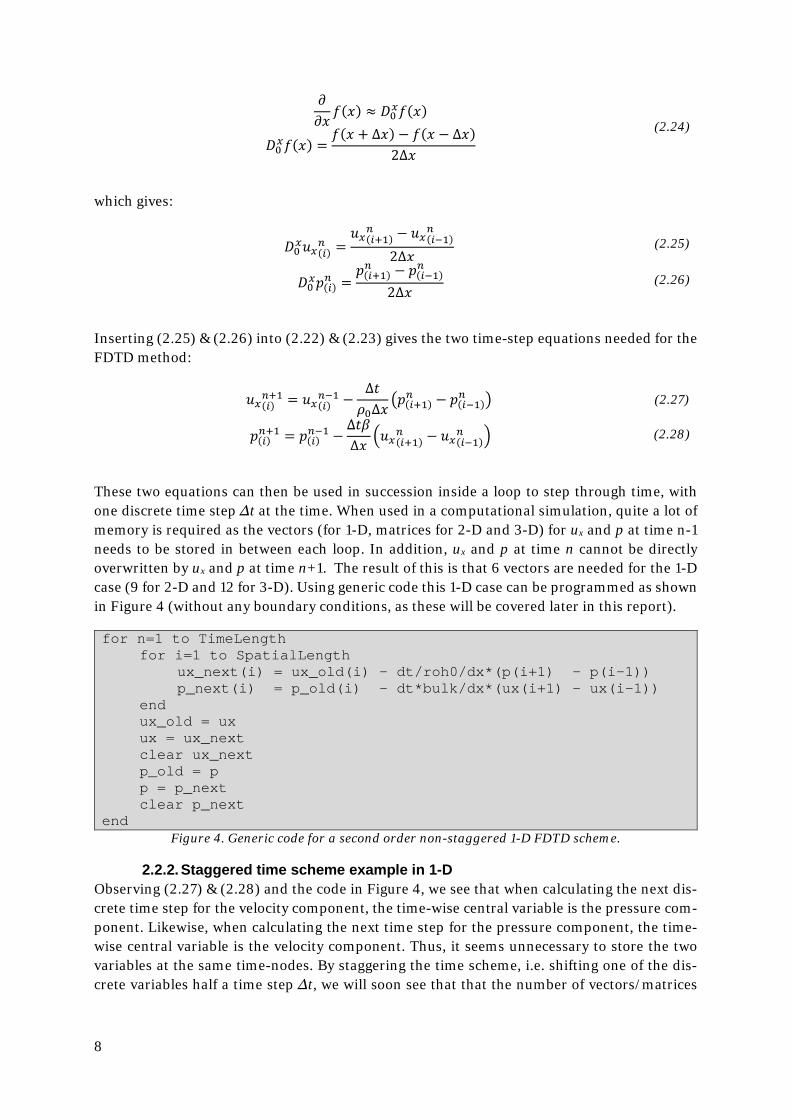
These two equations can then be used in succession inside a loop to step through time, with one discrete time step ∆t at the time. When used in a computational simulation, quite a lot of memory is required as the vectors (for 1-D, matrices for 2-D and 3-D) for ux and p at time n-1 needs to be stored in between each loop. In addition, ux and p at time n cannot be directly overwritten by ux and p at time n+1. The result of this is that 6 vectors are needed for the 1-D case (9 for 2-D and 12 for 3-D). Using generic code this 1-D case can be programmed as shown in Figure 4 (without any boundary conditions, as these will be covered later in this report).

for n=1 to TimeLength for i=1 to SpatialLength ux_next(i) = ux_old(i) – dt/roh0/dx*(p(i+1) - p(i-1)) p_next(i) = p_old(i) – dt*bulk/dx*(ux(i+1) - ux(i-1)) end ux_old = ux ux = ux_next clear ux_next p_old = p p = p_next clear p_next end

Figure 4. Generic code for a second order non-staggered 1-D FDTD scheme.

2.2.2. Staggered time scheme example in 1-D Observing (2.27) & (2.28) and the code in Figure 4, we see that when calculating the next dis-crete time step for the velocity component, the time-wise central variable is the pressure com-ponent. Likewise, when calculating the next time step for the pressure component, the time-wise central variable is the velocity component. Thus, it seems unnecessary to store the two variables at the same time-nodes. By staggering the time scheme, i.e. shifting one of the dis-crete variables half a time step ∆t, we will soon see that that the number of vectors/matrices

9

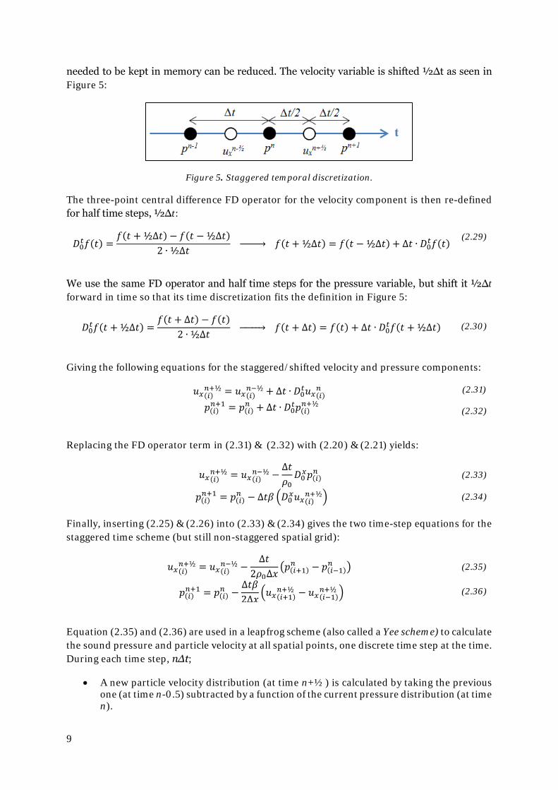
needed to be kept in memory can be reduced. The velocity variable is shifted ½∆t as seen in Figure 5:

Figure 5. Staggered temporal discretization.

The three-point central difference FD operator for the velocity component is then re-defined for half time steps, ½∆t:

𝐷𝐷0𝑡𝑡𝑓𝑓(𝜕𝜕) =𝑓𝑓(𝜕𝜕 + ½∆𝜕𝜕) − 𝑓𝑓(𝜕𝜕 − ½∆𝜕𝜕)

2 ∙ ½∆𝜕𝜕

�⎯⎯⎯⎯� 𝑓𝑓(𝜕𝜕 + ½∆𝜕𝜕) = 𝑓𝑓(𝜕𝜕 − ½∆𝜕𝜕) + ∆𝜕𝜕 ∙ 𝐷𝐷0𝑡𝑡𝑓𝑓(𝜕𝜕)

(2.29)

We use the same FD operator and half time steps for the pressure variable, but shift it ½∆t forward in time so that its time discretization fits the definition in Figure 5:

𝐷𝐷0𝑡𝑡𝑓𝑓(𝜕𝜕 + ½∆𝜕𝜕) =𝑓𝑓(𝜕𝜕 + ∆𝜕𝜕) − 𝑓𝑓(𝜕𝜕)

2 ∙ ½∆𝜕𝜕

�⎯⎯⎯⎯� 𝑓𝑓(𝜕𝜕 + ∆𝜕𝜕) = 𝑓𝑓(𝜕𝜕) + ∆𝜕𝜕 ∙ 𝐷𝐷0𝑡𝑡𝑓𝑓(𝜕𝜕 + ½∆𝜕𝜕) (2.30)

Giving the following equations for the staggered/shifted velocity and pressure components:

𝑢𝑢𝑥𝑥(𝑖𝑖)𝑛𝑛+½ = 𝑢𝑢𝑥𝑥(𝑖𝑖)

𝑛𝑛−½ + ∆𝜕𝜕 ∙ 𝐷𝐷0𝑡𝑡𝑢𝑢𝑥𝑥(𝑖𝑖)𝑛𝑛


𝑛𝑛 + ∆𝜕𝜕 ∙ 𝐷𝐷0𝑡𝑡𝑝𝑝(𝑖𝑖)𝑛𝑛+½

(2.31)

(2.32)

Replacing the FD operator term in (2.31) & (2.32) with (2.20) & (2.21) yields:


𝑛𝑛−½ −∆𝜕𝜕𝜌𝜌0𝐷𝐷0𝑥𝑥𝑝𝑝(𝑖𝑖)

𝑛𝑛 (2.33)


𝑛𝑛 − ∆𝜕𝜕𝛽𝛽 �𝐷𝐷0𝑥𝑥𝑢𝑢𝑥𝑥(𝑖𝑖)𝑛𝑛+½� (2.34)

Finally, inserting (2.25) & (2.26) into (2.33) & (2.34) gives the two time-step equations for the staggered time scheme (but still non-staggered spatial grid):


𝑛𝑛−½ −∆𝜕𝜕

2𝜌𝜌0∆𝜕𝜕�𝑝𝑝(𝑖𝑖+1)

𝑛𝑛 − 𝑝𝑝(𝑖𝑖−1)𝑛𝑛 � (2.35)


𝑛𝑛 −∆𝜕𝜕𝛽𝛽2∆𝜕𝜕

�𝑢𝑢𝑥𝑥(𝑖𝑖+1)𝑛𝑛+½ − 𝑢𝑢𝑥𝑥(𝑖𝑖−1)

𝑛𝑛+½ � (2.36)

Equation (2.35) and (2.36) are used in a leapfrog scheme (also called a Yee scheme) to calculate the sound pressure and particle velocity at all spatial points, one discrete time step at the time. During each time step, n∆t;

• A new particle velocity distribution (at time n+½) is calculated by taking the previous one (at time n-0.5) subtracted by a function of the current pressure distribution (at time n).

10

• A new sound pressure distribution (at time n+1) is calculated by taking the previous one (at time n) subtracted by a function of the current particle velocity distribution (at time n+½).

The scheme is looped until the desired time duration of the simulation is reached. In compu-tational simulations, the sound pressure and/or particle velocity distribution (or any other quantity based on the knowledge of these two) can be visualized in each time step. It should be noted that it is not necessary to keep the previous distributions in memory, so only 2 vectors are needed for the 1-D case (3 for 2-D and 4 for 3-D). Using generic code this 1-D case can be programmed like in Figure 6 (again without any boundary conditions).

for n=1 to TimeLength for i=1 to SpatialLength ux(i) = ux(i) – dt/roh0/2/dx*(p(i+1) - p(i-1)) p(i) = p(i) – dt*bulk/2/dx*(ux(i+1) - ux(i-1)) end end

Figure 6. Generic code for a second order 1-D FDTD scheme, staggered in time but not in space.

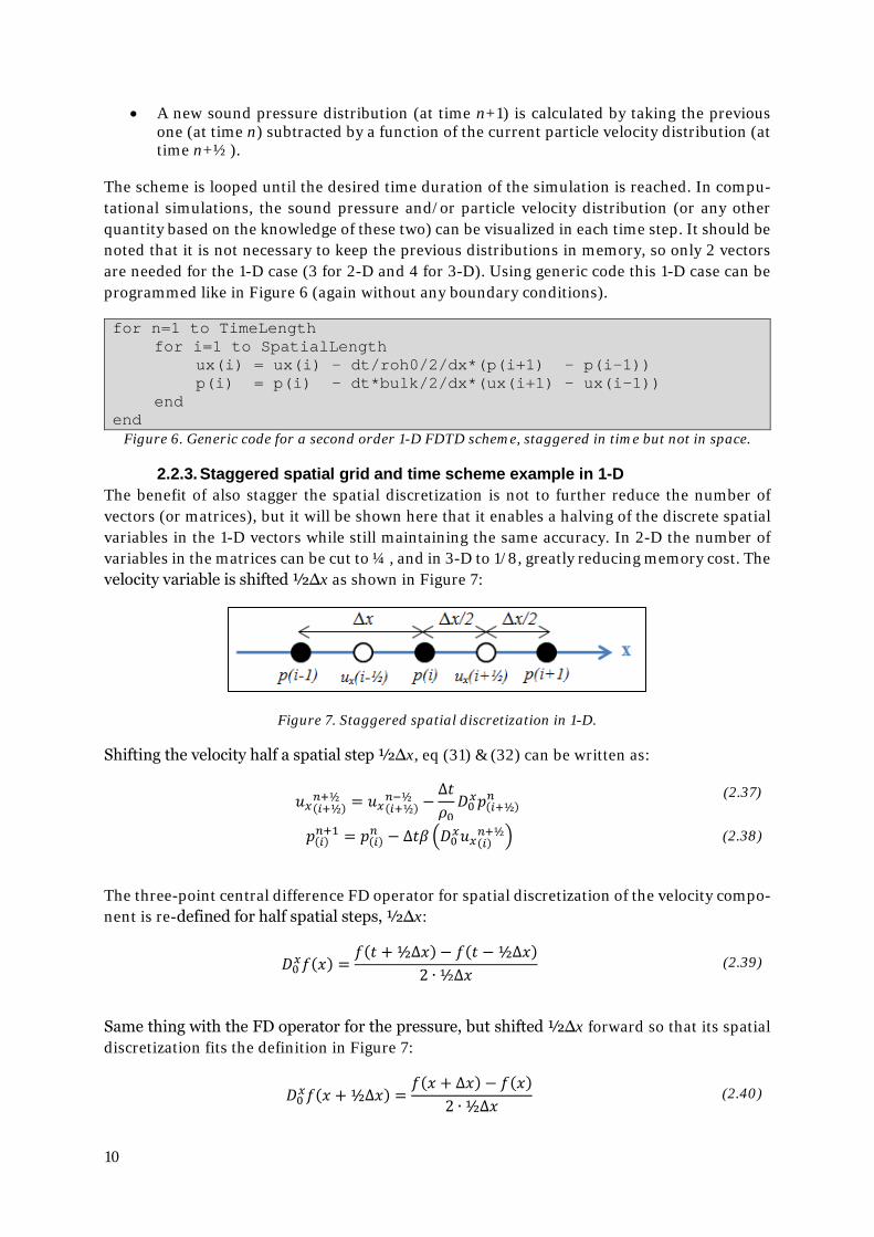
2.2.3. Staggered spatial grid and time scheme example in 1-D The benefit of also stagger the spatial discretization is not to further reduce the number of vectors (or matrices), but it will be shown here that it enables a halving of the discrete spatial variables in the 1-D vectors while still maintaining the same accuracy. In 2-D the number of variables in the matrices can be cut to ¼, and in 3-D to 1/8, greatly reducing memory cost. The velocity variable is shifted ½∆x as shown in Figure 7:

Figure 7. Staggered spatial discretization in 1-D.

Shifting the velocity half a spatial step ½∆x, eq (31) & (32) can be written as:

𝑢𝑢𝑥𝑥(𝑖𝑖+½)𝑛𝑛+½ = 𝑢𝑢𝑥𝑥(𝑖𝑖+½)

𝑛𝑛−½ −∆𝜕𝜕𝜌𝜌0𝐷𝐷0𝑥𝑥𝑝𝑝(𝑖𝑖+½)

𝑛𝑛 (2.37)


𝑛𝑛 − ∆𝜕𝜕𝛽𝛽 �𝐷𝐷0𝑥𝑥𝑢𝑢𝑥𝑥(𝑖𝑖)𝑛𝑛+½� (2.38)

The three-point central difference FD operator for spatial discretization of the velocity compo-nent is re-defined for half spatial steps, ½∆x:

𝐷𝐷0𝑥𝑥𝑓𝑓(𝜕𝜕) =𝑓𝑓(𝜕𝜕 + ½∆𝜕𝜕)− 𝑓𝑓(𝜕𝜕 − ½∆𝜕𝜕)

2 ∙ ½∆𝜕𝜕 (2.39)

Same thing with the FD operator for the pressure, but shifted ½∆x forward so that its spatial discretization fits the definition in Figure 7:

𝐷𝐷0𝑥𝑥𝑓𝑓(𝜕𝜕 + ½∆𝜕𝜕) =𝑓𝑓(𝜕𝜕 + ∆𝜕𝜕) − 𝑓𝑓(𝜕𝜕)

2 ∙ ½∆𝜕𝜕 (2.40)

11

Which gives:

𝐷𝐷0𝑥𝑥𝑢𝑢𝑥𝑥(𝑖𝑖)𝑛𝑛+½ =

𝑢𝑢𝑥𝑥(𝑖𝑖+½)𝑛𝑛+½ − 𝑢𝑢𝑥𝑥(𝑖𝑖−½)

𝑛𝑛+½

∆𝜕𝜕 (2.41)

𝐷𝐷0𝑥𝑥𝑝𝑝(𝑖𝑖+½)𝑛𝑛 =

𝑝𝑝(𝑖𝑖+1)𝑛𝑛 − 𝑝𝑝(𝑖𝑖)

𝑛𝑛

∆𝜕𝜕 (2.42)

Inserting (2.41) & (2.42) into (2.37) & (2.38) gives the two time-step equations for the stag-gered (in space and time) 1-D FDTD scheme:

𝑢𝑢𝑥𝑥(𝑖𝑖+½)𝑛𝑛+½ = 𝑢𝑢𝑥𝑥(𝑖𝑖+½)

𝑛𝑛−½ −∆𝜕𝜕𝜌𝜌0∆𝜕𝜕

�𝑝𝑝(𝑖𝑖+1)𝑛𝑛 − 𝑝𝑝(𝑖𝑖)

𝑛𝑛 � (2.43)


𝑛𝑛 −∆𝜕𝜕𝛽𝛽∆𝜕𝜕

�𝑢𝑢𝑥𝑥(𝑖𝑖+½)𝑛𝑛+½ − 𝑢𝑢𝑥𝑥(𝑖𝑖−½)

𝑛𝑛+½ � (2.44)

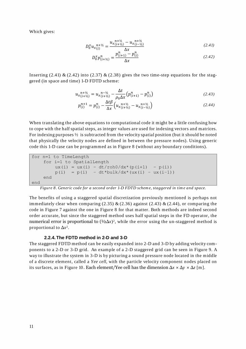
When translating the above equations to computational code it might be a little confusing how to cope with the half spatial steps, as integer values are used for indexing vectors and matrices. For indexing purposes ½ is subtracted from the velocity spatial position (but it should be noted that physically the velocity nodes are defined in between the pressure nodes). Using generic code this 1-D case can be programmed as in Figure 8 (without any boundary conditions).

for n=1 to TimeLength for i=1 to SpatialLength ux(i) = ux(i) – dt/roh0/dx*(p(i+1) - p(i)) p(i) = p(i) – dt*bulk/dx*(ux(i) - ux(i-1)) end end

Figure 8. Generic code for a second order 1-D FDTD scheme, staggered in time and space.

The benefits of using a staggered spatial discretization previously mentioned is perhaps not immediately clear when comparing (2.35) & (2.36) against (2.43) & (2.44), or comparing the code in Figure 7 against the one in Figure 8 for that matter. Both methods are indeed second order accurate, but since the staggered method uses half spatial steps in the FD operator, the numerical error is proportional to (½∆x)2, while the error using the un-staggered method is proportional to ∆x2.

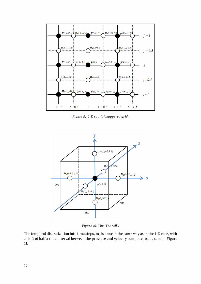
2.2.4. The FDTD method in 2-D and 3-D The staggered FDTD method can be easily expanded into 2-D and 3-D by adding velocity com-ponents to a 2-D or 3-D grid. An example of a 2-D staggered grid can be seen in Figure 9. A way to illustrate the system in 3-D is by picturing a sound pressure node located in the middle of a discrete element, called a Yee cell, with the particle velocity component nodes placed on its surfaces, as in Figure 10. Each element/Yee cell has the dimension ∆x × ∆y × ∆z [m].

12

Figure 9. 2-D spatial staggered grid.

Figure 10. The “Yee cell”.

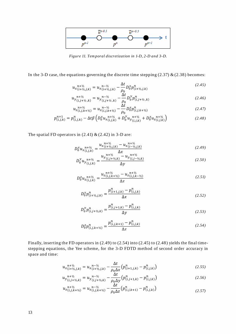
The temporal discretization into time steps, ∆t, is done in the same way as in the 1-D case, with a shift of half a time interval between the pressure and velocity components, as seen in Figure 11.

13

Figure 11. Temporal discretization in 1-D, 2-D and 3-D.

In the 3-D case, the equations governing the discrete time stepping (2.37) & (2.38) becomes:

𝑢𝑢𝑥𝑥(𝑖𝑖+½,𝑗𝑗,𝑘𝑘)𝑛𝑛+½ = 𝑢𝑢𝑥𝑥(𝑖𝑖+½,𝑗𝑗,𝑘𝑘)

𝑛𝑛−½ −∆𝜕𝜕𝜌𝜌0𝐷𝐷0𝑥𝑥𝑝𝑝(𝑖𝑖+½,𝑗𝑗,𝑘𝑘)

𝑛𝑛 (2.45)

𝑢𝑢𝑦𝑦(𝑖𝑖,𝑗𝑗+½ ,𝑘𝑘)𝑛𝑛+½ = 𝑢𝑢𝑦𝑦(𝑖𝑖,𝑗𝑗+½ ,𝑘𝑘)

𝑛𝑛−½ −∆𝜕𝜕𝜌𝜌0𝐷𝐷0𝑦𝑦𝑝𝑝(𝑖𝑖,𝑗𝑗+½ ,𝑘𝑘)

𝑛𝑛 (2.46)

𝑢𝑢𝑧𝑧(𝑖𝑖,𝑗𝑗,𝑘𝑘+½)𝑛𝑛+½ = 𝑢𝑢𝑧𝑧(𝑖𝑖,𝑗𝑗,𝑘𝑘+½)

𝑛𝑛−½ −∆𝜕𝜕𝜌𝜌0𝐷𝐷0𝑧𝑧𝑝𝑝(𝑖𝑖,𝑗𝑗,𝑘𝑘+½)

𝑛𝑛 (2.47)

𝑝𝑝(𝑖𝑖,𝑗𝑗,𝑘𝑘)𝑛𝑛+1 = 𝑝𝑝(𝑖𝑖,𝑗𝑗,𝑘𝑘)

𝑛𝑛 − ∆𝜕𝜕𝛽𝛽 �𝐷𝐷0𝑥𝑥𝑢𝑢𝑥𝑥(𝑖𝑖,𝑗𝑗,𝑘𝑘)𝑛𝑛+½ + 𝐷𝐷0

𝑦𝑦𝑢𝑢𝑦𝑦(𝑖𝑖,𝑗𝑗,𝑘𝑘)𝑛𝑛+½ + 𝐷𝐷0𝑧𝑧𝑢𝑢𝑧𝑧(𝑖𝑖,𝑗𝑗,𝑘𝑘)

𝑛𝑛+½ � (2.48)

The spatial FD operators in (2.41) & (2.42) in 3-D are:

𝐷𝐷0𝑥𝑥𝑢𝑢𝑥𝑥(𝑖𝑖,𝑗𝑗,𝑘𝑘)𝑛𝑛+½ =

𝑢𝑢𝑥𝑥(𝑖𝑖+½,𝑗𝑗,𝑘𝑘)𝑛𝑛+½ − 𝑢𝑢𝑥𝑥(𝑖𝑖−½,𝑗𝑗,𝑘𝑘)

𝑛𝑛+½

∆𝜕𝜕 (2.49)

𝐷𝐷0𝑦𝑦𝑢𝑢𝑦𝑦(𝑖𝑖,𝑗𝑗,𝑘𝑘)

𝑛𝑛+½ =𝑢𝑢𝑦𝑦(𝑖𝑖,𝑗𝑗+½,𝑘𝑘)

𝑛𝑛+½ − 𝑢𝑢𝑦𝑦(𝑖𝑖,𝑗𝑗−½,𝑘𝑘)𝑛𝑛+½

∆𝜕𝜕 (2.50)

𝐷𝐷0𝑧𝑧𝑢𝑢𝑧𝑧(𝑖𝑖,𝑗𝑗,𝑘𝑘)𝑛𝑛+½ =

𝑢𝑢𝑧𝑧(𝑖𝑖,𝑗𝑗,𝑘𝑘+½)𝑛𝑛+½ − 𝑢𝑢𝑧𝑧(𝑖𝑖,𝑗𝑗,𝑘𝑘−½)

𝑛𝑛+½

∆𝜕𝜕 (2.51)

𝐷𝐷0𝑥𝑥𝑝𝑝(𝑖𝑖+½,𝑗𝑗,𝑘𝑘)𝑛𝑛 =

𝑝𝑝(𝑖𝑖+1,𝑗𝑗,𝑘𝑘)𝑛𝑛 − 𝑝𝑝(𝑖𝑖,𝑗𝑗,𝑘𝑘)

𝑛𝑛

∆𝜕𝜕

(2.52)

𝐷𝐷0𝑦𝑦𝑝𝑝(𝑖𝑖,𝑗𝑗+½,𝑘𝑘)

𝑛𝑛 =𝑝𝑝(𝑖𝑖,𝑗𝑗+1,𝑘𝑘)𝑛𝑛 − 𝑝𝑝(𝑖𝑖,𝑗𝑗,𝑘𝑘)

𝑛𝑛

∆𝜕𝜕

(2.53)

𝐷𝐷0𝑧𝑧𝑝𝑝(𝑖𝑖,𝑗𝑗,𝑘𝑘+½)𝑛𝑛 =

𝑝𝑝(𝑖𝑖,𝑗𝑗,𝑘𝑘+1)𝑛𝑛 − 𝑝𝑝(𝑖𝑖,𝑗𝑗,𝑘𝑘)

𝑛𝑛

∆𝜕𝜕 (2.54)

Finally, inserting the FD operators in (2.49) to (2.54) into (2.45) to (2.48) yields the final time-stepping equations, the Yee scheme, for the 3-D FDTD method of second order accuracy in space and time:


𝑛𝑛−½ −∆𝜕𝜕𝜌𝜌0∆𝜕𝜕

�𝑝𝑝(𝑖𝑖+1,𝑗𝑗,𝑘𝑘)𝑛𝑛 − 𝑝𝑝(𝑖𝑖,𝑗𝑗,𝑘𝑘)

𝑛𝑛 � (2.55)

𝑢𝑢𝑦𝑦(𝑖𝑖,𝑗𝑗+½,𝑘𝑘)𝑛𝑛+½ = 𝑢𝑢𝑦𝑦(𝑖𝑖,𝑗𝑗+½,𝑘𝑘)

𝑛𝑛−½ −∆𝜕𝜕𝜌𝜌0∆𝜕𝜕

�𝑝𝑝(𝑖𝑖,𝑗𝑗+1,𝑘𝑘)𝑛𝑛 − 𝑝𝑝(𝑖𝑖,𝑗𝑗,𝑘𝑘)

𝑛𝑛 � (2.56)


𝑛𝑛−½ −∆𝜕𝜕𝜌𝜌0∆𝜕𝜕

�𝑝𝑝(𝑖𝑖,𝑗𝑗,𝑘𝑘+1)𝑛𝑛 − 𝑝𝑝(𝑖𝑖,𝑗𝑗,𝑘𝑘)

𝑛𝑛 �

(2.57)

14


𝑛𝑛 − ∆𝜕𝜕𝛽𝛽 �𝑢𝑢𝑥𝑥(𝑖𝑖+½,𝑗𝑗,𝑘𝑘)

𝑛𝑛+½ − 𝑢𝑢𝑥𝑥(𝑖𝑖−½,𝑗𝑗,𝑘𝑘)𝑛𝑛+½

∆𝜕𝜕+𝑢𝑢𝑦𝑦(𝑖𝑖,𝑗𝑗+½,𝑘𝑘)

𝑛𝑛+½ − 𝑢𝑢𝑦𝑦(𝑖𝑖,𝑗𝑗−½,𝑘𝑘)𝑛𝑛+½

∆𝜕𝜕

+𝑢𝑢𝑧𝑧(𝑖𝑖,𝑗𝑗,𝑘𝑘+½)

𝑛𝑛+½ − 𝑢𝑢𝑧𝑧(𝑖𝑖,𝑗𝑗,𝑘𝑘−½)𝑛𝑛+½

∆𝜕𝜕�

(2.58)

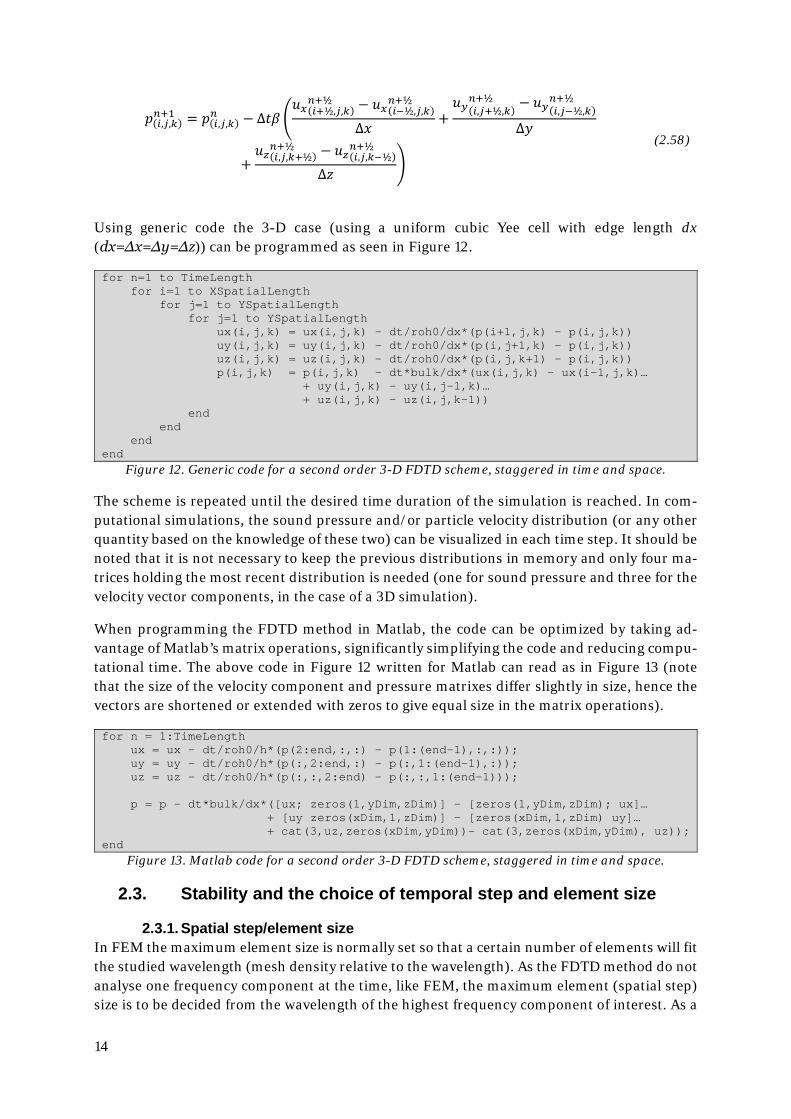
Using generic code the 3-D case (using a uniform cubic Yee cell with edge length dx (dx=∆x=∆y=∆z)) can be programmed as seen in Figure 12.

for n=1 to TimeLength for i=1 to XSpatialLength for j=1 to YSpatialLength for j=1 to YSpatialLength ux(i,j,k) = ux(i,j,k) – dt/roh0/dx*(p(i+1,j,k) - p(i,j,k)) uy(i,j,k) = uy(i,j,k) – dt/roh0/dx*(p(i,j+1,k) - p(i,j,k)) uz(i,j,k) = uz(i,j,k) – dt/roh0/dx*(p(i,j,k+1) - p(i,j,k)) p(i,j,k) = p(i,j,k) – dt*bulk/dx*(ux(i,j,k) - ux(i-1,j,k)… + uy(i,j,k) - uy(i,j-1,k)… + uz(i,j,k) - uz(i,j,k-1)) end end end end

Figure 12. Generic code for a second order 3-D FDTD scheme, staggered in time and space.

The scheme is repeated until the desired time duration of the simulation is reached. In com-putational simulations, the sound pressure and/or particle velocity distribution (or any other quantity based on the knowledge of these two) can be visualized in each time step. It should be noted that it is not necessary to keep the previous distributions in memory and only four ma-trices holding the most recent distribution is needed (one for sound pressure and three for the velocity vector components, in the case of a 3D simulation).

When programming the FDTD method in Matlab, the code can be optimized by taking ad-vantage of Matlab’s matrix operations, significantly simplifying the code and reducing compu-tational time. The above code in Figure 12 written for Matlab can read as in Figure 13 (note that the size of the velocity component and pressure matrixes differ slightly in size, hence the vectors are shortened or extended with zeros to give equal size in the matrix operations).

for n = 1:TimeLength ux = ux - dt/roh0/h*(p(2:end,:,:) - p(1:(end-1),:,:)); uy = uy - dt/roh0/h*(p(:,2:end,:) - p(:,1:(end-1),:)); uz = uz - dt/roh0/h*(p(:,:,2:end) - p(:,:,1:(end-1))); p = p - dt*bulk/dx*([ux; zeros(1,yDim,zDim)] - [zeros(1,yDim,zDim); ux]… + [uy zeros(xDim,1,zDim)] - [zeros(xDim,1,zDim) uy]… + cat(3,uz,zeros(xDim,yDim))- cat(3,zeros(xDim,yDim), uz)); end

Figure 13. Matlab code for a second order 3-D FDTD scheme, staggered in time and space.

2.3. Stability and the choice of temporal step and element size

2.3.1. Spatial step/element size In FEM the maximum element size is normally set so that a certain number of elements will fit the studied wavelength (mesh density relative to the wavelength). As the FDTD method do not analyse one frequency component at the time, like FEM, the maximum element (spatial step) size is to be decided from the wavelength of the highest frequency component of interest. As a

15

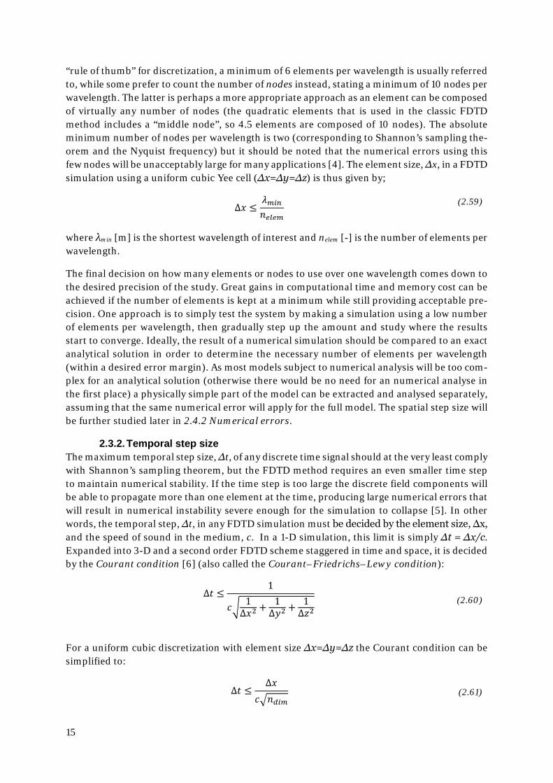
“rule of thumb” for discretization, a minimum of 6 elements per wavelength is usually referred to, while some prefer to count the number of nodes instead, stating a minimum of 10 nodes per wavelength. The latter is perhaps a more appropriate approach as an element can be composed of virtually any number of nodes (the quadratic elements that is used in the classic FDTD method includes a “middle node”, so 4.5 elements are composed of 10 nodes). The absolute minimum number of nodes per wavelength is two (corresponding to Shannon’s sampling the-orem and the Nyquist frequency) but it should be noted that the numerical errors using this few nodes will be unacceptably large for many applications [4]. The element size, ∆x, in a FDTD simulation using a uniform cubic Yee cell (∆x=∆y=∆z) is thus given by;

∆𝜕𝜕 ≤𝜆𝜆𝑡𝑡𝑖𝑖𝑛𝑛

𝑛𝑛𝑡𝑡𝑒𝑒𝑡𝑡𝑡𝑡 (2.59)

where λmin [m] is the shortest wavelength of interest and nelem [-] is the number of elements per wavelength.

The final decision on how many elements or nodes to use over one wavelength comes down to the desired precision of the study. Great gains in computational time and memory cost can be achieved if the number of elements is kept at a minimum while still providing acceptable pre-cision. One approach is to simply test the system by making a simulation using a low number of elements per wavelength, then gradually step up the amount and study where the results start to converge. Ideally, the result of a numerical simulation should be compared to an exact analytical solution in order to determine the necessary number of elements per wavelength (within a desired error margin). As most models subject to numerical analysis will be too com-plex for an analytical solution (otherwise there would be no need for an numerical analyse in the first place) a physically simple part of the model can be extracted and analysed separately, assuming that the same numerical error will apply for the full model. The spatial step size will be further studied later in 2.4.2 Numerical errors.

2.3.2. Temporal step size The maximum temporal step size, ∆t, of any discrete time signal should at the very least comply with Shannon’s sampling theorem, but the FDTD method requires an even smaller time step to maintain numerical stability. If the time step is too large the discrete field components will be able to propagate more than one element at the time, producing large numerical errors that will result in numerical instability severe enough for the simulation to collapse [5]. In other words, the temporal step, ∆t, in any FDTD simulation must be decided by the element size, ∆x, and the speed of sound in the medium, c. In a 1-D simulation, this limit is simply ∆t = ∆x/c. Expanded into 3-D and a second order FDTD scheme staggered in time and space, it is decided by the Courant condition [6] (also called the Courant–Friedrichs–Lewy condition):

∆𝜕𝜕 ≤1

𝑐𝑐� 1∆𝜕𝜕2 + 1

∆𝜕𝜕2 + 1∆𝜕𝜕2

(2.60)

For a uniform cubic discretization with element size ∆x=∆y=∆z the Courant condition can be simplified to:

∆𝜕𝜕 ≤∆𝜕𝜕

𝑐𝑐�𝑛𝑛𝑑𝑑𝑖𝑖𝑡𝑡 (2.61)

16

where ndim [-] is the number of dimensions.

Assuming that the maximum allowed element size from (2.59) is used, the maximum temporal step size can be calculated from:

∆𝜕𝜕 ≤1

𝑓𝑓𝑡𝑡𝑚𝑚𝑥𝑥 ∙ 𝑛𝑛𝑡𝑡𝑒𝑒𝑡𝑡𝑡𝑡 ∙ �𝑛𝑛𝑑𝑑𝑖𝑖𝑡𝑡 (2.62)

where fmax [Hz] is the highest frequency component of interest.

It should be noted that the Courant condition applies for free propagation and will not neces-sarily work after adding boundary conditions to the simulation.

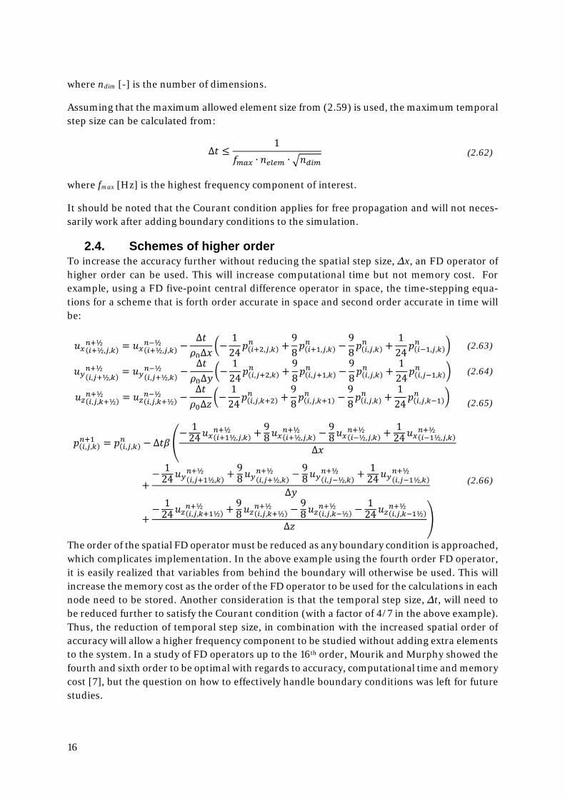
2.4. Schemes of higher order To increase the accuracy further without reducing the spatial step size, ∆x, an FD operator of higher order can be used. This will increase computational time but not memory cost. For example, using a FD five-point central difference operator in space, the time-stepping equa-tions for a scheme that is forth order accurate in space and second order accurate in time will be:


𝑛𝑛−½ −∆𝜕𝜕𝜌𝜌0∆𝜕𝜕

�−1

24𝑝𝑝(𝑖𝑖+2,𝑗𝑗,𝑘𝑘)𝑛𝑛 +

98𝑝𝑝(𝑖𝑖+1,𝑗𝑗,𝑘𝑘)𝑛𝑛 −

98𝑝𝑝(𝑖𝑖,𝑗𝑗,𝑘𝑘)𝑛𝑛 +

124

𝑝𝑝(𝑖𝑖−1,𝑗𝑗,𝑘𝑘)𝑛𝑛 � (2.63)

𝑢𝑢𝑦𝑦(𝑖𝑖,𝑗𝑗+½,𝑘𝑘)𝑛𝑛+½ = 𝑢𝑢𝑦𝑦(𝑖𝑖,𝑗𝑗+½,𝑘𝑘)

𝑛𝑛−½ −∆𝜕𝜕𝜌𝜌0∆𝜕𝜕

�−1

24𝑝𝑝(𝑖𝑖,𝑗𝑗+2,𝑘𝑘)𝑛𝑛 +

98𝑝𝑝(𝑖𝑖,𝑗𝑗+1,𝑘𝑘)𝑛𝑛 −


124

𝑝𝑝(𝑖𝑖,𝑗𝑗−1,𝑘𝑘)𝑛𝑛 � (2.64)


𝑛𝑛−½ −∆𝜕𝜕𝜌𝜌0∆𝜕𝜕

�−1

24𝑝𝑝(𝑖𝑖,𝑗𝑗,𝑘𝑘+2)𝑛𝑛 +

98𝑝𝑝(𝑖𝑖,𝑗𝑗,𝑘𝑘+1)𝑛𝑛 −


124

𝑝𝑝(𝑖𝑖,𝑗𝑗,𝑘𝑘−1)𝑛𝑛 �

(2.65)


𝑛𝑛 − ∆𝜕𝜕𝛽𝛽 �− 1

24𝑢𝑢𝑥𝑥(𝑖𝑖+1½,𝑗𝑗,𝑘𝑘)𝑛𝑛+½ + 9

8𝑢𝑢𝑥𝑥(𝑖𝑖+½,𝑗𝑗,𝑘𝑘)𝑛𝑛+½ − 9

8𝑢𝑢𝑥𝑥(𝑖𝑖−½,𝑗𝑗,𝑘𝑘)𝑛𝑛+½ + 1

24𝑢𝑢𝑥𝑥(𝑖𝑖−1½,𝑗𝑗,𝑘𝑘)𝑛𝑛+½

∆𝜕𝜕

+− 1

24𝑢𝑢𝑦𝑦(𝑖𝑖,𝑗𝑗+1½,𝑘𝑘)𝑛𝑛+½ + 9

8𝑢𝑢𝑦𝑦(𝑖𝑖,𝑗𝑗+½,𝑘𝑘)𝑛𝑛+½ − 9

8𝑢𝑢𝑦𝑦(𝑖𝑖,𝑗𝑗−½,𝑘𝑘)𝑛𝑛+½ + 1

24𝑢𝑢𝑦𝑦(𝑖𝑖,𝑗𝑗−1½,𝑘𝑘)𝑛𝑛+½

∆𝜕𝜕

+− 1

24𝑢𝑢𝑧𝑧(𝑖𝑖,𝑗𝑗,𝑘𝑘+1½)𝑛𝑛+½ + 9

8𝑢𝑢𝑧𝑧(𝑖𝑖,𝑗𝑗,𝑘𝑘+½)𝑛𝑛+½ − 9

8𝑢𝑢𝑧𝑧(𝑖𝑖,𝑗𝑗,𝑘𝑘−½)𝑛𝑛+½ − 1

24𝑢𝑢𝑧𝑧(𝑖𝑖,𝑗𝑗,𝑘𝑘−1½)𝑛𝑛+½

∆𝜕𝜕�

(2.66)

The order of the spatial FD operator must be reduced as any boundary condition is approached, which complicates implementation. In the above example using the fourth order FD operator, it is easily realized that variables from behind the boundary will otherwise be used. This will increase the memory cost as the order of the FD operator to be used for the calculations in each node need to be stored. Another consideration is that the temporal step size, ∆t, will need to be reduced further to satisfy the Courant condition (with a factor of 4/7 in the above example). Thus, the reduction of temporal step size, in combination with the increased spatial order of accuracy will allow a higher frequency component to be studied without adding extra elements to the system. In a study of FD operators up to the 16th order, Mourik and Murphy showed the fourth and sixth order to be optimal with regards to accuracy, computational time and memory cost [7], but the question on how to effectively handle boundary conditions was left for future studies.

17

For the purpose of this thesis, the benefits of using FD operators of higher than second order accuracy is small, as the purpose is to investigate low frequencies with large wavelengths. Thus, increasing the accuracy of the FDTD model beyond second order accuracy will provide minimal gains in accuracy for an increased computational time and memory cost.

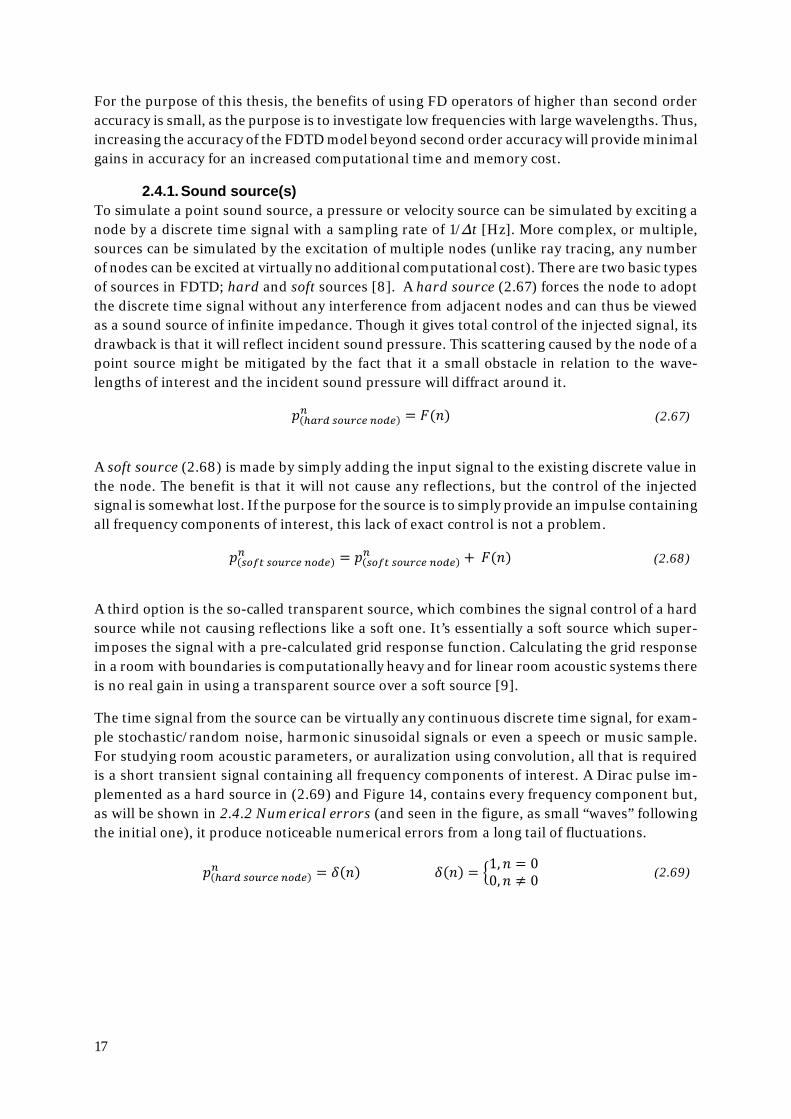
2.4.1. Sound source(s) To simulate a point sound source, a pressure or velocity source can be simulated by exciting a node by a discrete time signal with a sampling rate of 1/∆t [Hz]. More complex, or multiple, sources can be simulated by the excitation of multiple nodes (unlike ray tracing, any number of nodes can be excited at virtually no additional computational cost). There are two basic types of sources in FDTD; hard and soft sources [8]. A hard source (2.67) forces the node to adopt the discrete time signal without any interference from adjacent nodes and can thus be viewed as a sound source of infinite impedance. Though it gives total control of the injected signal, its drawback is that it will reflect incident sound pressure. This scattering caused by the node of a point source might be mitigated by the fact that it a small obstacle in relation to the wave-lengths of interest and the incident sound pressure will diffract around it.

𝑝𝑝(ℎ𝑚𝑚𝐸𝐸𝑑𝑑 𝑡𝑡𝐸𝐸𝑠𝑠𝐸𝐸𝑠𝑠𝑡𝑡 𝑛𝑛𝐸𝐸𝑑𝑑𝑡𝑡)𝑛𝑛 = 𝐹𝐹(𝑛𝑛) (2.67)

A soft source (2.68) is made by simply adding the input signal to the existing discrete value in the node. The benefit is that it will not cause any reflections, but the control of the injected signal is somewhat lost. If the purpose for the source is to simply provide an impulse containing all frequency components of interest, this lack of exact control is not a problem.

𝑝𝑝(𝑡𝑡𝐸𝐸𝑠𝑠𝑡𝑡 𝑡𝑡𝐸𝐸𝑠𝑠𝐸𝐸𝑠𝑠𝑡𝑡 𝑛𝑛𝐸𝐸𝑑𝑑𝑡𝑡)𝑛𝑛 = 𝑝𝑝(𝑡𝑡𝐸𝐸𝑠𝑠𝑡𝑡 𝑡𝑡𝐸𝐸𝑠𝑠𝐸𝐸𝑠𝑠𝑡𝑡 𝑛𝑛𝐸𝐸𝑑𝑑𝑡𝑡)

𝑛𝑛 + 𝐹𝐹(𝑛𝑛) (2.68)

A third option is the so-called transparent source, which combines the signal control of a hard source while not causing reflections like a soft one. It’s essentially a soft source which super-imposes the signal with a pre-calculated grid response function. Calculating the grid response in a room with boundaries is computationally heavy and for linear room acoustic systems there is no real gain in using a transparent source over a soft source [9].

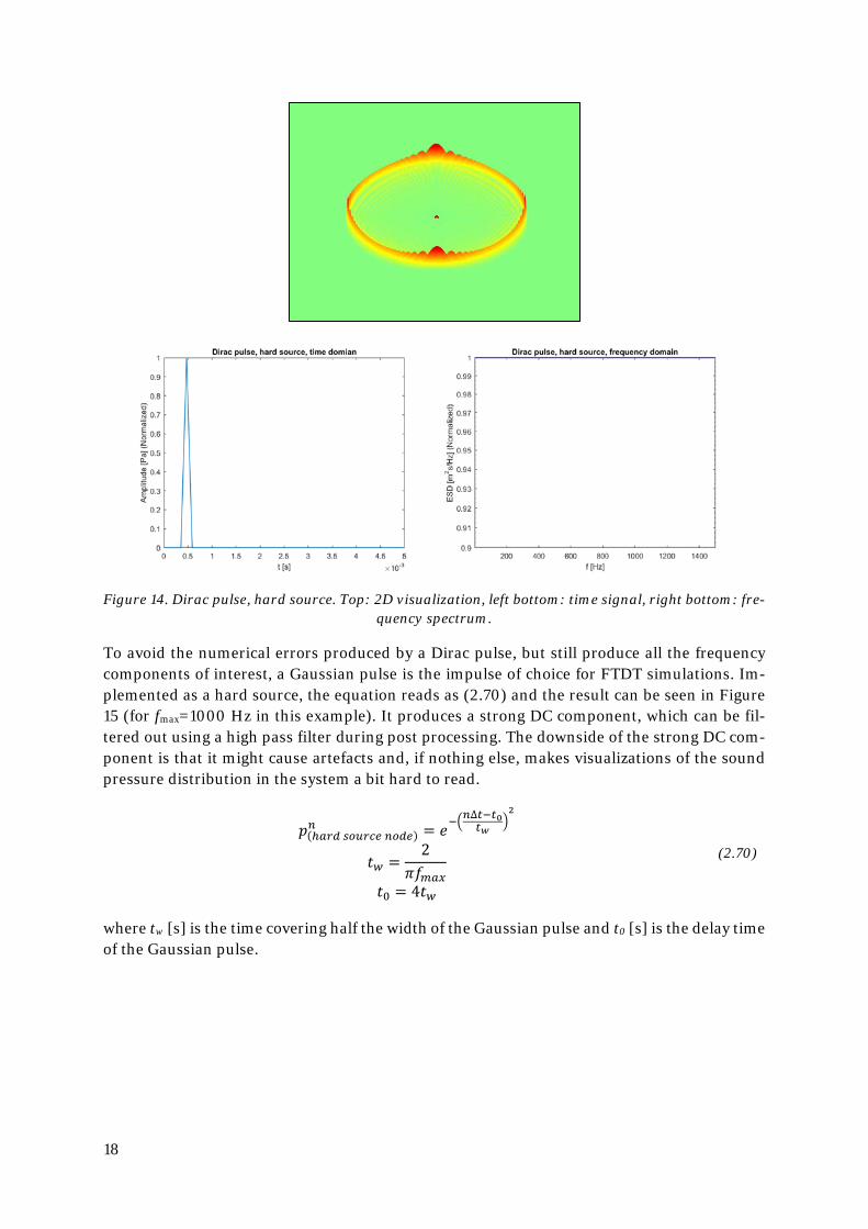
The time signal from the source can be virtually any continuous discrete time signal, for exam-ple stochastic/random noise, harmonic sinusoidal signals or even a speech or music sample. For studying room acoustic parameters, or auralization using convolution, all that is required is a short transient signal containing all frequency components of interest. A Dirac pulse im-plemented as a hard source in (2.69) and Figure 14, contains every frequency component but, as will be shown in 2.4.2 Numerical errors (and seen in the figure, as small “waves” following the initial one), it produce noticeable numerical errors from a long tail of fluctuations.

𝑝𝑝(ℎ𝑚𝑚𝐸𝐸𝑑𝑑 𝑡𝑡𝐸𝐸𝑠𝑠𝐸𝐸𝑠𝑠𝑡𝑡 𝑛𝑛𝐸𝐸𝑑𝑑𝑡𝑡)𝑛𝑛 = 𝛿𝛿(𝑛𝑛) 𝛿𝛿(𝑛𝑛) = �1,𝑛𝑛 = 0

0,𝑛𝑛 ≠ 0 (2.69)

18

Figure 14. Dirac pulse, hard source. Top: 2D visualization, left bottom: time signal, right bottom: fre-quency spectrum.

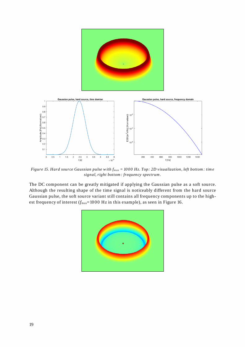
To avoid the numerical errors produced by a Dirac pulse, but still produce all the frequency components of interest, a Gaussian pulse is the impulse of choice for FTDT simulations. Im-plemented as a hard source, the equation reads as (2.70) and the result can be seen in Figure 15 (for fmax=1000 Hz in this example). It produces a strong DC component, which can be fil-tered out using a high pass filter during post processing. The downside of the strong DC com-ponent is that it might cause artefacts and, if nothing else, makes visualizations of the sound pressure distribution in the system a bit hard to read.

𝑝𝑝(ℎ𝑚𝑚𝐸𝐸𝑑𝑑 𝑡𝑡𝐸𝐸𝑠𝑠𝐸𝐸𝑠𝑠𝑡𝑡 𝑛𝑛𝐸𝐸𝑑𝑑𝑡𝑡)𝑛𝑛 = 𝑒𝑒−�

𝑛𝑛∆𝑡𝑡−𝑡𝑡0𝑡𝑡𝑤𝑤

�2

𝜕𝜕𝑤𝑤 =2

𝜋𝜋𝑓𝑓𝑡𝑡𝑚𝑚𝑥𝑥

𝜕𝜕0 = 4𝜕𝜕𝑤𝑤

(2.70)

where tw [s] is the time covering half the width of the Gaussian pulse and t0 [s] is the delay time of the Gaussian pulse.

19

Figure 15. Hard source Gaussian pulse with fmax = 1000 Hz. Top: 2D visualization, left bottom: time signal, right bottom: frequency spectrum.

The DC component can be greatly mitigated if applying the Gaussian pulse as a soft source. Although the resulting shape of the time signal is noticeably different from the hard source Gaussian pulse, the soft source variant still contains all frequency components up to the high-est frequency of interest (fmax=1000 Hz in this example), as seen in Figure 16.

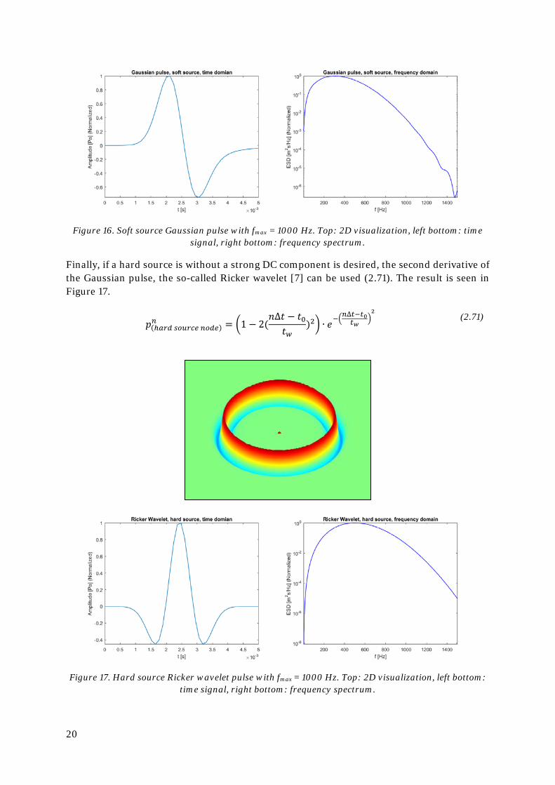
20

Figure 16. Soft source Gaussian pulse with fmax = 1000 Hz. Top: 2D visualization, left bottom: time signal, right bottom: frequency spectrum.

Finally, if a hard source is without a strong DC component is desired, the second derivative of the Gaussian pulse, the so-called Ricker wavelet [7] can be used (2.71). The result is seen in Figure 17.

𝑝𝑝(ℎ𝑚𝑚𝐸𝐸𝑑𝑑 𝑡𝑡𝐸𝐸𝑠𝑠𝐸𝐸𝑠𝑠𝑡𝑡 𝑛𝑛𝐸𝐸𝑑𝑑𝑡𝑡)𝑛𝑛 = �1 − 2(

𝑛𝑛∆𝜕𝜕 − 𝜕𝜕0𝜕𝜕𝑤𝑤

)2� ∙ 𝑒𝑒−�𝑛𝑛∆𝑡𝑡−𝑡𝑡0𝑡𝑡𝑤𝑤

�2

(2.71)

Figure 17. Hard source Ricker wavelet pulse with fmax = 1000 Hz. Top: 2D visualization, left bottom: time signal, right bottom: frequency spectrum.

21

2.4.2. Numerical errors As previously mentioned, using second order accuracy in space and time will cause numerical errors dominated by the third derivative of space and time respectively (proportional to ∆x2 and ∆t2). In a 1-D simulation these two errors will cancel out if ∆t is set to the maximum allowed value by the Courant condition, but when performing 2-D or 3-D simulations they will not cancel out and will cause dispersive errors. These numerical error causes the phase and group velocities among the frequency components to differ, leading to frequency components prop-agating at different speeds [6]. In other words, the speed of sound is no longer the constant c = ω/k but dependent on frequency. The error appears to be the strongest for waves propagating along the Cartesian axes and the weakest when propagating along its diagonals. For a uniform staggered Cartesian grid the numerical error will get severe and cause large dissipation for high enough frequency components, where the spatial discretization gets too coarse (or when reach-ing the Nyquist frequency). The phase error for a wave propagating along one of the Cartesian axes can be calculated using [10]:

𝜑𝜑𝐹𝐹𝐹𝐹𝐹𝐹𝐹𝐹𝜑𝜑𝐴𝐴𝑛𝑛𝑚𝑚𝑒𝑒𝑦𝑦𝑡𝑡𝑖𝑖𝑠𝑠𝑚𝑚𝑒𝑒

= �2arcsin (𝑐𝑐∆𝜕𝜕�𝑠𝑠𝑖𝑖𝑛𝑛2(𝑘𝑘∆𝜕𝜕/2)/∆𝜕𝜕2

𝑐𝑐∆𝜕𝜕√𝑘𝑘2�𝑛𝑛

(2.72)

Along the diagonal, the phase will change according to:

𝜑𝜑𝐹𝐹𝐹𝐹𝐹𝐹𝐹𝐹𝜑𝜑𝐴𝐴𝑛𝑛𝑚𝑚𝑒𝑒𝑦𝑦𝑡𝑡𝑖𝑖𝑠𝑠𝑚𝑚𝑒𝑒

=

⎝

⎛2arcsin (𝑐𝑐∆𝜕𝜕�3𝑠𝑠𝑖𝑖𝑛𝑛2(𝑘𝑘/�3/∆𝜕𝜕/2)/∆𝜕𝜕2

𝑐𝑐∆𝜕𝜕√𝑘𝑘2⎠

⎞

𝑛𝑛

(2.73)

where k [1/m] is the wavenumber of the frequency in question and n [-] is the number of time steps taken.

For auralization purposes, these phase errors will appear as a high frequency “ringing” which should naturally be avoided if a natural sound is desired. For this reason, an upper frequency range “headroom” is required to be able to filter out these artefacts using a low pass filter dur-ing post processing.

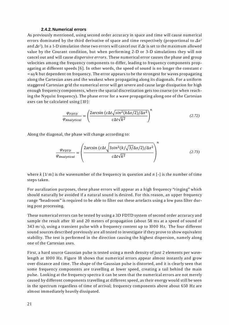
These numerical errors can be tested by using a 3D FDTD system of second order accuracy and sample the result after 10 and 20 meters of propagation (about 58 ms at a speed of sound of 343 m/s), using a transient pulse with a frequency content up to 1000 Hz. The four different sound sources described previously are all tested to investigate if they prove to show equivalent stability. The test is performed in the direction causing the highest dispersion, namely along one of the Cartesian axes.

First, a hard source Gaussian pulse is tested using a mesh density of just 2 elements per wave-length at 1000 Hz. Figure 18 shows that numerical errors appear almost instantly and grow over distance and time. The shape of the Gaussian pulse is distorted, and it is clearly seen that some frequency components are travelling at lower speed, creating a tail behind the main pulse. Looking at the frequency spectra it can be seen that the numerical errors are not merely caused by different components travelling at different speed, as their energy would still be seen in the spectrum regardless of time of arrival; frequency components above about 650 Hz are almost immediately heavily dissipated.

22

Figure 18. Hard source Gaussian pulse with 2 elements/wavelength at 1000 Hz. Left: time signal, right: frequency spectrum.

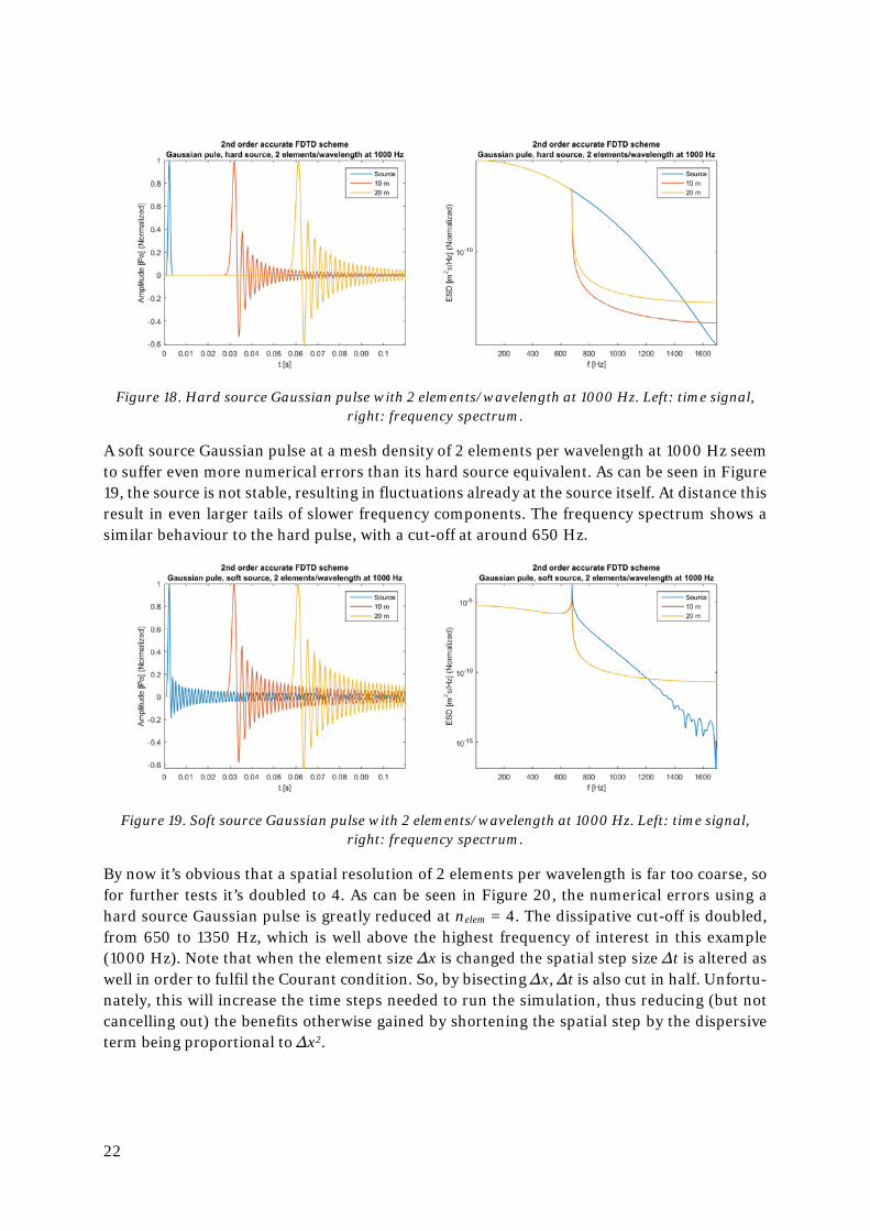
A soft source Gaussian pulse at a mesh density of 2 elements per wavelength at 1000 Hz seem to suffer even more numerical errors than its hard source equivalent. As can be seen in Figure 19, the source is not stable, resulting in fluctuations already at the source itself. At distance this result in even larger tails of slower frequency components. The frequency spectrum shows a similar behaviour to the hard pulse, with a cut-off at around 650 Hz.

Figure 19. Soft source Gaussian pulse with 2 elements/wavelength at 1000 Hz. Left: time signal, right: frequency spectrum.

By now it’s obvious that a spatial resolution of 2 elements per wavelength is far too coarse, so for further tests it’s doubled to 4. As can be seen in Figure 20, the numerical errors using a hard source Gaussian pulse is greatly reduced at nelem = 4. The dissipative cut-off is doubled, from 650 to 1350 Hz, which is well above the highest frequency of interest in this example (1000 Hz). Note that when the element size ∆x is changed the spatial step size ∆t is altered as well in order to fulfil the Courant condition. So, by bisecting ∆x, ∆t is also cut in half. Unfortu-nately, this will increase the time steps needed to run the simulation, thus reducing (but not cancelling out) the benefits otherwise gained by shortening the spatial step by the dispersive term being proportional to ∆x2.

23

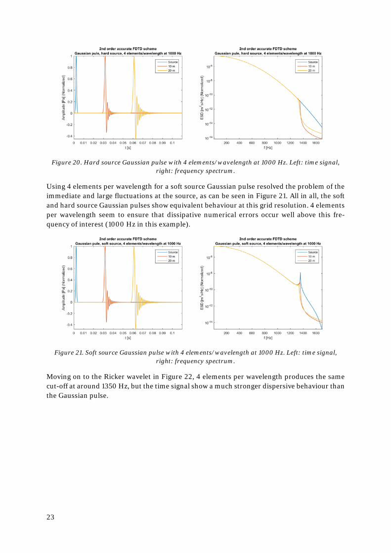
Figure 20. Hard source Gaussian pulse with 4 elements/wavelength at 1000 Hz. Left: time signal, right: frequency spectrum.

Using 4 elements per wavelength for a soft source Gaussian pulse resolved the problem of the immediate and large fluctuations at the source, as can be seen in Figure 21. All in all, the soft and hard source Gaussian pulses show equivalent behaviour at this grid resolution. 4 elements per wavelength seem to ensure that dissipative numerical errors occur well above this fre-quency of interest (1000 Hz in this example).

Figure 21. Soft source Gaussian pulse with 4 elements/wavelength at 1000 Hz. Left: time signal, right: frequency spectrum.

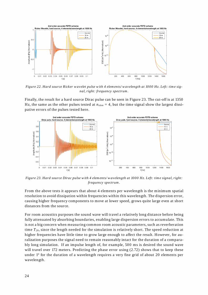
Moving on to the Ricker wavelet in Figure 22, 4 elements per wavelength produces the same cut-off at around 1350 Hz, but the time signal show a much stronger dispersive behaviour than the Gaussian pulse.

24

Figure 22. Hard source Ricker wavelet pulse with 4 elements/wavelength at 1000 Hz. Left: time sig-nal, right: frequency spectrum.

Finally, the result for a hard source Dirac pulse can be seen in Figure 23. The cut-off is at 1350 Hz, the same as the other pulses tested at nelem = 4, but the time signal show the largest dissi-pative errors of the pulses tested here.

Figure 23. Hard source Dirac pulse with 4 elements/wavelength at 1000 Hz. Left: time signal, right: frequency spectrum.

From the above tests it appears that about 4 elements per wavelength is the minimum spatial resolution to avoid dissipation within frequencies within this wavelength. The dispersion error, causing higher frequency components to move at lower speed, grows quite large even at short distances from the source.

For room acoustics purposes the sound wave will travel a relatively long distance before being fully attenuated by absorbing boundaries, enabling large dispersion errors to accumulate. This is not a big concern when measuring common room acoustic parameters, such as reverberation time T20, since the length needed for the simulation is relatively short. The speed reduction at higher frequencies have little time to grow large enough to affect the result. However, for au-ralization purposes the signal need to remain reasonably intact for the duration of a compara-bly long simulation. If an impulse length of, for example, 500 ms is desired the sound wave will travel over 172 meters. Predicting the phase error using (2.72) shows that to keep these under 1° for the duration of a wavelength requires a very fine grid of about 20 elements per wavelength.

25

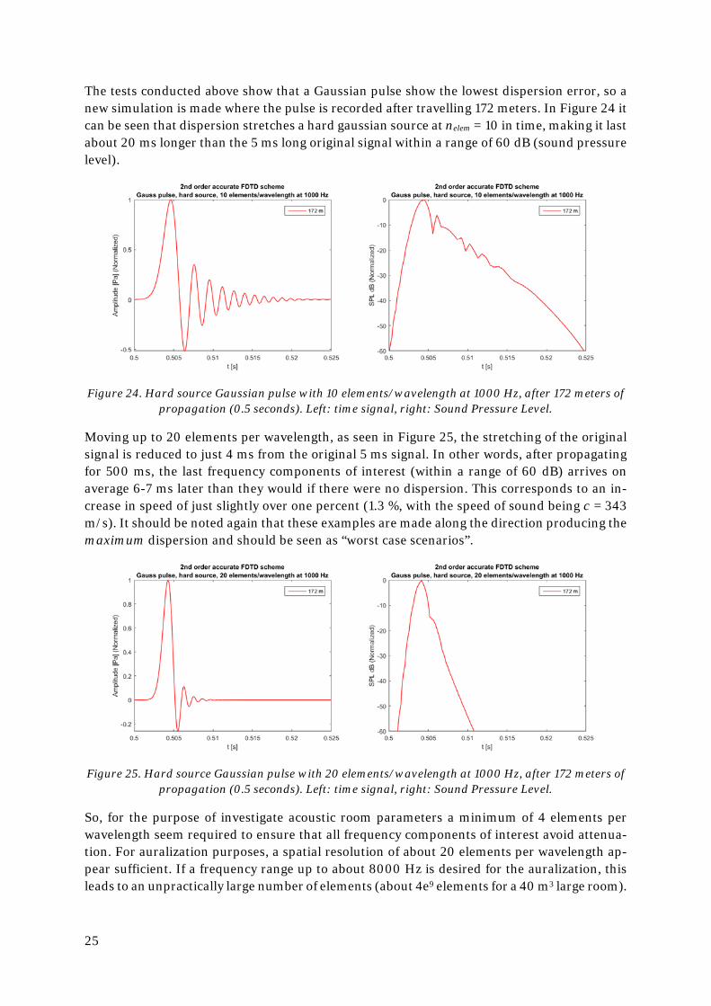
The tests conducted above show that a Gaussian pulse show the lowest dispersion error, so a new simulation is made where the pulse is recorded after travelling 172 meters. In Figure 24 it can be seen that dispersion stretches a hard gaussian source at nelem = 10 in time, making it last about 20 ms longer than the 5 ms long original signal within a range of 60 dB (sound pressure level).

Figure 24. Hard source Gaussian pulse with 10 elements/wavelength at 1000 Hz, after 172 meters of propagation (0.5 seconds). Left: time signal, right: Sound Pressure Level.

Moving up to 20 elements per wavelength, as seen in Figure 25, the stretching of the original signal is reduced to just 4 ms from the original 5 ms signal. In other words, after propagating for 500 ms, the last frequency components of interest (within a range of 60 dB) arrives on average 6-7 ms later than they would if there were no dispersion. This corresponds to an in-crease in speed of just slightly over one percent (1.3 %, with the speed of sound being c = 343 m/s). It should be noted again that these examples are made along the direction producing the maximum dispersion and should be seen as “worst case scenarios”.

Figure 25. Hard source Gaussian pulse with 20 elements/wavelength at 1000 Hz, after 172 meters of propagation (0.5 seconds). Left: time signal, right: Sound Pressure Level.

So, for the purpose of investigate acoustic room parameters a minimum of 4 elements per wavelength seem required to ensure that all frequency components of interest avoid attenua-tion. For auralization purposes, a spatial resolution of about 20 elements per wavelength ap-pear sufficient. If a frequency range up to about 8000 Hz is desired for the auralization, this leads to an unpractically large number of elements (about 4e9 elements for a 40 m3 large room).

26

3. Boundary conditions When a sound wave travel from one medium and reach the surface of another, i.e. reaches a boundary, the relationship between the sound pressure and particle velocity is typically de-scribed by the specific acoustic surface normal impedance Zn [Pa•s/m] [3]:

𝑍𝑍𝑛𝑛 =𝑝𝑝

𝑢𝑢�⃗ ∙ 𝑛𝑛�⃗ (3.1)

where n [-] is the normal of the surface

The most basic type of boundary condition; a perfectly rigid wall, has infinite acoustic surface normal impedance resulting in zero particle velocity at the surface. Modelling a perfectly rigid boundary condition is thus as easy as permanently assigning zero velocity to the velocity nodes at the boundary. In a FDTD model this boundary condition is “automatically” assigned to the end nodes of the simulated fluid domain, as the particle velocity is always zero outside the matrix. Implementing any real-numbered impedance is quite straight forward, but a frequency dependent boundary requires a complex numbered specific acoustic surface normal imped-ance (from now on called just “impedance” for short):

𝑍𝑍𝑛𝑛(𝑓𝑓) = 𝑍𝑍𝑅𝑅 + 𝑖𝑖𝑍𝑍𝐼𝐼(𝑓𝑓) (3.2)

where ZR [Pa•s/m] is the resistive part and ZI [Pa•s/m] the frequency dependent reactive part.

The direct use a complex component for the impedance in a FDTD model is not possible for two reasons; 1) all variables in the FDTD scheme need to be real-numbered, and 2) the discrete sound wave can potentially contain any number of frequency components, thus elimination the possibility to use a frequency dependent reactive part of the impedance. The incident sound wave will hit the boundary one sample per time step, making it impossible to program a fre-quency dependent reactive function.

For room acoustics a versatile boundary condition is naturally desired and there exist a wide range of different ideas on how to best implement a frequency dependent impedance. The ear-liest method I found was from 1992 for electromagnetics studies using FDTD, where Sullivan published a method using Z-transforms [11]. The Z-transform approach has been investigated further for room acoustics applications by for example Jeong and Lam in 2010 [12]. Suzuki et al proposed in a 2006 paper a more hands-on method by simply assigning the density, speed of sound and flow resistance on the bordering medium [13]. The drawback of such method is that to satisfy the Courant condition the global time step of the simulation must be set accord-ing to the medium with the highest speed of sound, in most cases drastically increasing the number of time steps needed. In his first paper on acoustic FDTD methods in 1993, Bottel-dooren describes a method based on a simple complex impedance with a reactive part directly proportional to the frequency [2], and expands it further in a later paper in 1995 [10]. The boundary condition suggested by Botteldooren is essentially a 1-DOF mass, spring and damper system, which might seem a little crude compared to the use of Z-transforms or the 2-DOF system later published by Sakamoto et al. in 2008 [14], but for simulating only a limited range of low frequencies it could prove sufficient. Since it’s easily implemented in a matrix based Matlab code without any big changes to the time stepping scheme and doesn’t require a large number of new matrices for storing the boundary condition parameters, it’s investigated fur-ther as the basic boundary condition in this thesis. This 1-DOF boundary condition is locally

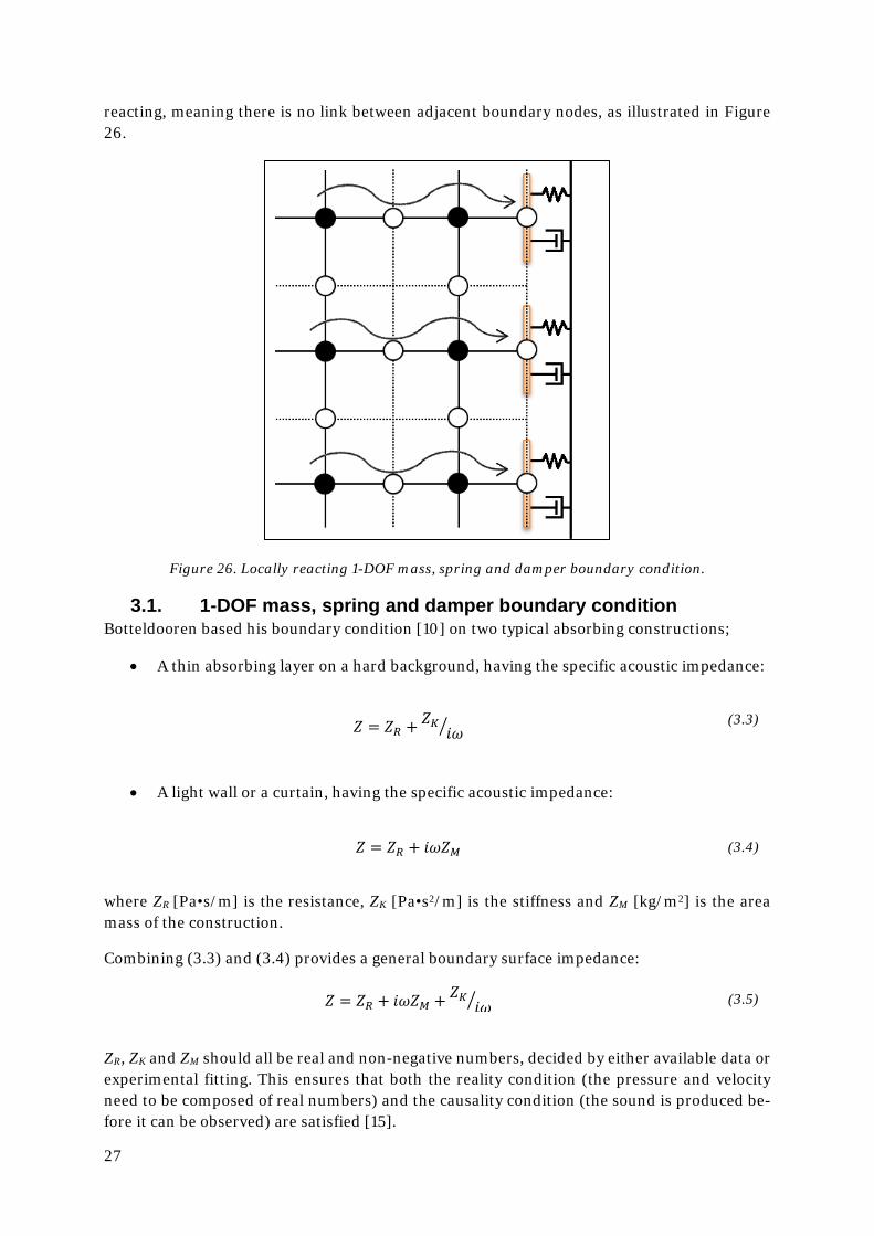
27

reacting, meaning there is no link between adjacent boundary nodes, as illustrated in Figure 26.

Figure 26. Locally reacting 1-DOF mass, spring and damper boundary condition.

3.1. 1-DOF mass, spring and damper boundary condition Botteldooren based his boundary condition [10] on two typical absorbing constructions;

• A thin absorbing layer on a hard background, having the specific acoustic impedance:

𝑍𝑍 = 𝑍𝑍𝑅𝑅 + 𝑍𝑍𝐾𝐾𝑖𝑖𝑖𝑖� (3.3)

• A light wall or a curtain, having the specific acoustic impedance:

𝑍𝑍 = 𝑍𝑍𝑅𝑅 + 𝑖𝑖𝑖𝑖𝑍𝑍𝑀𝑀 (3.4)

where ZR [Pa•s/m] is the resistance, ZK [Pa•s2/m] is the stiffness and ZM [kg/m2] is the area mass of the construction.

Combining (3.3) and (3.4) provides a general boundary surface impedance:

𝑍𝑍 = 𝑍𝑍𝑅𝑅 + 𝑖𝑖𝑖𝑖𝑍𝑍𝑀𝑀 + 𝑍𝑍𝐾𝐾𝑖𝑖𝑖𝑖� (3.5)

ZR, ZK and ZM should all be real and non-negative numbers, decided by either available data or experimental fitting. This ensures that both the reality condition (the pressure and velocity need to be composed of real numbers) and the causality condition (the sound is produced be-fore it can be observed) are satisfied [15].

28

To implement this surface impedance in the time domain of a FDTD system, the relationship between pressure, velocity and impedance at one discrete point is:

𝑝𝑝(𝜕𝜕) = 𝑢𝑢�⃗ (𝜕𝜕) ∙ 𝑍𝑍 = 𝑍𝑍𝑅𝑅𝑢𝑢�⃗ (𝜕𝜕) + 𝑖𝑖𝑖𝑖𝑍𝑍𝑀𝑀𝑢𝑢�⃗ (𝜕𝜕) + 𝑍𝑍𝐾𝐾𝑢𝑢�⃗ (𝜕𝜕)𝑖𝑖𝑖𝑖� (3.6)

Assuming harmonic propagation gives:

𝑢𝑢�⃗ (𝜕𝜕) = 𝑢𝑢�𝑒𝑒𝑖𝑖𝑖𝑖𝑡𝑡 ∙ 𝑛𝑛�⃗ (3.7)

𝑑𝑑𝑢𝑢�⃗ (𝜕𝜕)𝑑𝑑𝜕𝜕

= 𝑖𝑖𝑖𝑖𝑢𝑢�𝑒𝑒𝑖𝑖𝑖𝑖𝑡𝑡 ∙ 𝑛𝑛�⃗ = 𝑖𝑖𝑖𝑖𝑢𝑢�⃗ (𝜕𝜕) (3.8)

� 𝑢𝑢�⃗ (𝜏𝜏)𝑑𝑑𝜏𝜏𝑡𝑡

−∞=𝑢𝑢�𝑒𝑒𝑖𝑖𝑖𝑖𝑡𝑡 ∙ 𝑛𝑛�⃗

𝑖𝑖𝑖𝑖=𝑢𝑢�⃗ (𝜕𝜕)𝑖𝑖𝑖𝑖

(3.9)

Inserting eq (3.8) and (3.9) into (3.6) gives:

𝑝𝑝(𝜕𝜕) = 𝑍𝑍𝑅𝑅𝑢𝑢�⃗ (𝜕𝜕) + 𝑍𝑍𝑀𝑀𝑑𝑑𝑢𝑢�⃗ (𝜕𝜕)𝑑𝑑𝜕𝜕

+ 𝑍𝑍𝐾𝐾 � 𝑢𝑢�⃗ (𝜏𝜏)𝑑𝑑𝜏𝜏𝑡𝑡

−∞ (3.10)

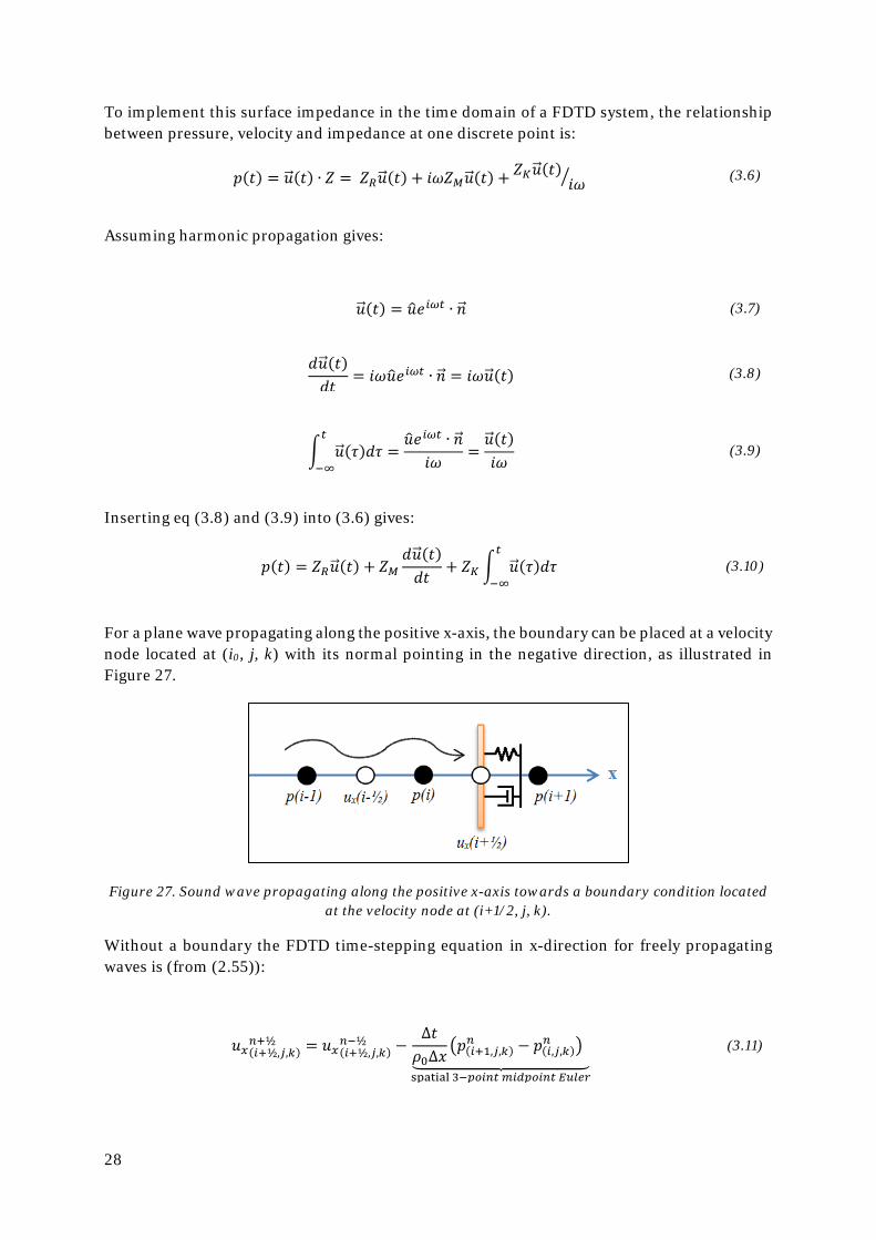
For a plane wave propagating along the positive x-axis, the boundary can be placed at a velocity node located at (i0, j, k) with its normal pointing in the negative direction, as illustrated in Figure 27.

Figure 27. Sound wave propagating along the positive x-axis towards a boundary condition located at the velocity node at (i+1/2, j, k).

Without a boundary the FDTD time-stepping equation in x-direction for freely propagating waves is (from (2.55)):


𝑛𝑛−½ −∆𝜕𝜕𝜌𝜌0∆𝜕𝜕

�𝑝𝑝(𝑖𝑖+1,𝑗𝑗,𝑘𝑘)𝑛𝑛 − 𝑝𝑝(𝑖𝑖,𝑗𝑗,𝑘𝑘)

𝑛𝑛 � ��spatial 3−𝑝𝑝𝐸𝐸𝑖𝑖𝑛𝑛𝑡𝑡 𝑡𝑡𝑖𝑖𝑑𝑑𝑝𝑝𝐸𝐸𝑖𝑖𝑛𝑛𝑡𝑡 𝐸𝐸𝑠𝑠𝑒𝑒𝑡𝑡𝐸𝐸

(3.11)

29

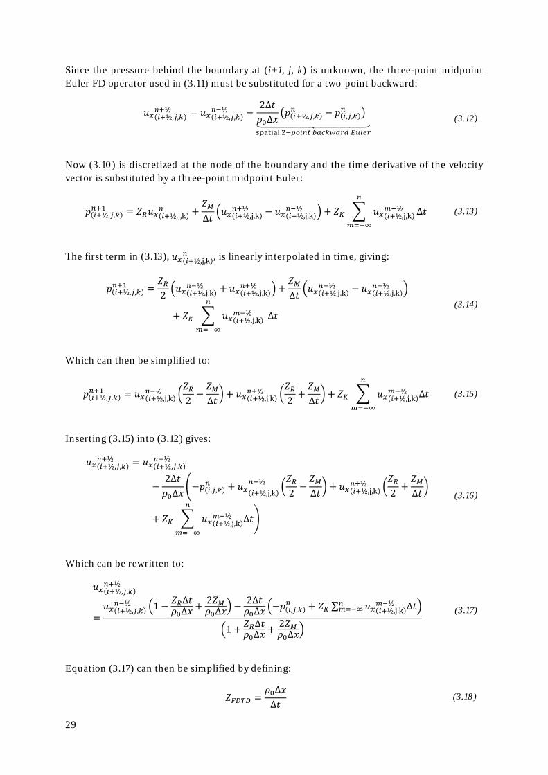
Since the pressure behind the boundary at (i+1, j, k) is unknown, the three-point midpoint Euler FD operator used in (3.11) must be substituted for a two-point backward:


𝑛𝑛−½ −2∆𝜕𝜕𝜌𝜌0∆𝜕𝜕

�𝑝𝑝(𝑖𝑖+½,𝑗𝑗,𝑘𝑘)𝑛𝑛 − 𝑝𝑝(𝑖𝑖,𝑗𝑗,𝑘𝑘)

𝑛𝑛 � ��spatial 2−𝑝𝑝𝐸𝐸𝑖𝑖𝑛𝑛𝑡𝑡 𝑏𝑏𝑚𝑚𝑠𝑠𝑘𝑘𝑤𝑤𝑚𝑚𝐸𝐸𝑑𝑑 𝐸𝐸𝑠𝑠𝑒𝑒𝑡𝑡𝐸𝐸

(3.12)

Now (3.10) is discretized at the node of the boundary and the time derivative of the velocity vector is substituted by a three-point midpoint Euler:

𝑝𝑝(𝑖𝑖+½,𝑗𝑗,𝑘𝑘)𝑛𝑛+1 = 𝑍𝑍𝑅𝑅𝑢𝑢𝑥𝑥(𝑖𝑖+½,j,k)

𝑛𝑛 +𝑍𝑍𝑀𝑀∆𝜕𝜕

�𝑢𝑢𝑥𝑥(𝑖𝑖+½,j,k)𝑛𝑛+½ − 𝑢𝑢𝑥𝑥(𝑖𝑖+½,j,k)

𝑛𝑛−½ �+ 𝑍𝑍𝐾𝐾 � 𝑢𝑢𝑥𝑥(𝑖𝑖+½,j,k)𝑡𝑡−½

𝑛𝑛

𝑡𝑡=−∞

∆𝜕𝜕 (3.13)

The first term in (3.13), 𝑢𝑢𝑥𝑥(𝑖𝑖+½,j,k)𝑛𝑛 , is linearly interpolated in time, giving:

𝑝𝑝(𝑖𝑖+½,𝑗𝑗,𝑘𝑘)𝑛𝑛+1 =

𝑍𝑍𝑅𝑅2�𝑢𝑢𝑥𝑥(𝑖𝑖+½,j,k)

𝑛𝑛−½ + 𝑢𝑢𝑥𝑥(𝑖𝑖+½,j,k)𝑛𝑛+½ �+

𝑍𝑍𝑀𝑀∆𝜕𝜕

�𝑢𝑢𝑥𝑥(𝑖𝑖+½,j,k)𝑛𝑛+½ − 𝑢𝑢𝑥𝑥(𝑖𝑖+½,j,k)

𝑛𝑛−½ �

+ 𝑍𝑍𝐾𝐾 � 𝑢𝑢𝑥𝑥(𝑖𝑖+½,j,k)𝑡𝑡−½

𝑛𝑛

𝑡𝑡=−∞

∆𝜕𝜕 (3.14)

Which can then be simplified to:

𝑝𝑝(𝑖𝑖+½,𝑗𝑗,𝑘𝑘)𝑛𝑛+1 = 𝑢𝑢𝑥𝑥(𝑖𝑖+½,j,k)

𝑛𝑛−½ �𝑍𝑍𝑅𝑅2−𝑍𝑍𝑀𝑀∆𝜕𝜕� + 𝑢𝑢𝑥𝑥(𝑖𝑖+½,j,k)

𝑛𝑛+½ �𝑍𝑍𝑅𝑅2

+𝑍𝑍𝑀𝑀∆𝜕𝜕� + 𝑍𝑍𝐾𝐾 � 𝑢𝑢𝑥𝑥(𝑖𝑖+½,j,k)

𝑡𝑡−½ ∆𝜕𝜕𝑛𝑛

𝑡𝑡=−∞

(3.15)

Inserting (3.15) into (3.12) gives:


𝑛𝑛−½

−2∆𝜕𝜕𝜌𝜌0∆𝜕𝜕

�−𝑝𝑝(𝑖𝑖,𝑗𝑗,𝑘𝑘)𝑛𝑛 + 𝑢𝑢𝑥𝑥(𝑖𝑖+½,j,k)

𝑛𝑛−½ �𝑍𝑍𝑅𝑅2−𝑍𝑍𝑀𝑀∆𝜕𝜕� + 𝑢𝑢𝑥𝑥(𝑖𝑖+½,j,k)

𝑛𝑛+½ �𝑍𝑍𝑅𝑅2

+𝑍𝑍𝑀𝑀∆𝜕𝜕�

+ 𝑍𝑍𝐾𝐾 � 𝑢𝑢𝑥𝑥(𝑖𝑖+½,j,k)𝑡𝑡−½ ∆𝜕𝜕

𝑛𝑛

𝑡𝑡=−∞

�

(3.16)

Which can be rewritten to:

𝑢𝑢𝑥𝑥(𝑖𝑖+½,𝑗𝑗,𝑘𝑘)𝑛𝑛+½

=𝑢𝑢𝑥𝑥(𝑖𝑖+½,𝑗𝑗,𝑘𝑘)

𝑛𝑛−½ �1 − 𝑍𝑍𝑅𝑅∆𝜕𝜕𝜌𝜌0∆𝜕𝜕

+ 2𝑍𝑍𝑀𝑀𝜌𝜌0∆𝜕𝜕

� − 2∆𝜕𝜕𝜌𝜌0∆𝜕𝜕

�−𝑝𝑝(𝑖𝑖,𝑗𝑗,𝑘𝑘)𝑛𝑛 + 𝑍𝑍𝐾𝐾 ∑ 𝑢𝑢𝑥𝑥(𝑖𝑖+½,j,k)

𝑡𝑡−½ ∆𝜕𝜕𝑛𝑛𝑡𝑡=−∞ �

�1 + 𝑍𝑍𝑅𝑅∆𝜕𝜕𝜌𝜌0∆𝜕𝜕

+ 2𝑍𝑍𝑀𝑀𝜌𝜌0∆𝜕𝜕

�

(3.17)

Equation (3.17) can then be simplified by defining:

𝑍𝑍𝐹𝐹𝐹𝐹𝐹𝐹𝐹𝐹 =𝜌𝜌0∆𝜕𝜕∆𝜕𝜕

(3.18)

30

𝛼𝛼 =1 − 𝑍𝑍𝑅𝑅

𝑍𝑍𝐹𝐹𝐹𝐹𝐹𝐹𝐹𝐹+ 2𝑍𝑍𝑀𝑀𝑍𝑍𝐹𝐹𝐹𝐹𝐹𝐹𝐹𝐹∆𝜕𝜕

1 + 𝑍𝑍𝑅𝑅𝑍𝑍𝐹𝐹𝐹𝐹𝐹𝐹𝐹𝐹

+ 2𝑍𝑍𝑀𝑀𝑍𝑍𝐹𝐹𝐹𝐹𝐹𝐹𝐹𝐹∆𝜕𝜕

(3.19)

𝛽𝛽 =2

1 + 𝑍𝑍𝑅𝑅𝑍𝑍𝐹𝐹𝐹𝐹𝐹𝐹𝐹𝐹

+ 2𝑍𝑍𝑀𝑀𝑍𝑍𝐹𝐹𝐹𝐹𝐹𝐹𝐹𝐹∆𝜕𝜕

(3.20)

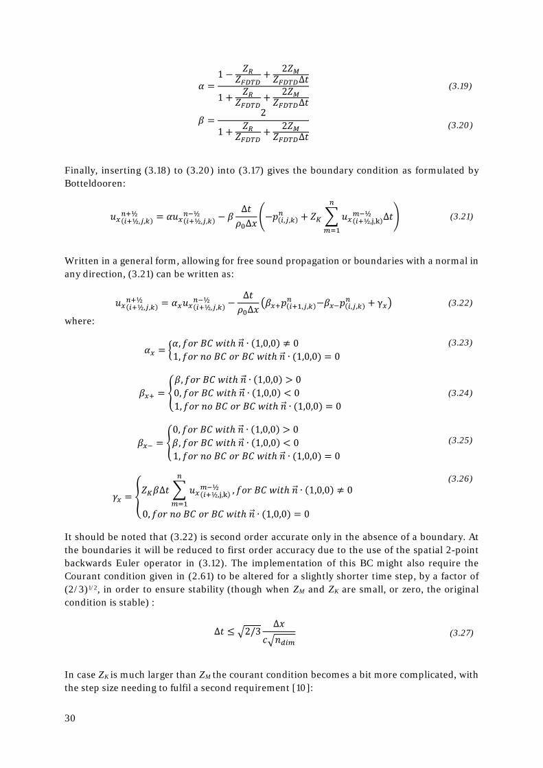
Finally, inserting (3.18) to (3.20) into (3.17) gives the boundary condition as formulated by Botteldooren:

𝑢𝑢𝑥𝑥(𝑖𝑖+½,𝑗𝑗,𝑘𝑘)𝑛𝑛+½ = 𝛼𝛼𝑢𝑢𝑥𝑥(𝑖𝑖+½,𝑗𝑗,𝑘𝑘)

𝑛𝑛−½ − 𝛽𝛽∆𝜕𝜕𝜌𝜌0∆𝜕𝜕

�−𝑝𝑝(𝑖𝑖,𝑗𝑗,𝑘𝑘)𝑛𝑛 + 𝑍𝑍𝐾𝐾 � 𝑢𝑢𝑥𝑥(𝑖𝑖+½,j,k)

𝑡𝑡−½ ∆𝜕𝜕𝑛𝑛

𝑡𝑡=1

� (3.21)

Written in a general form, allowing for free sound propagation or boundaries with a normal in any direction, (3.21) can be written as:

𝑢𝑢𝑥𝑥(𝑖𝑖+½,𝑗𝑗,𝑘𝑘)𝑛𝑛+½ = 𝛼𝛼𝑥𝑥𝑢𝑢𝑥𝑥(𝑖𝑖+½,𝑗𝑗,𝑘𝑘)

𝑛𝑛−½ −∆𝜕𝜕𝜌𝜌0∆𝜕𝜕

�𝛽𝛽𝑥𝑥+𝑝𝑝(𝑖𝑖+1,𝑗𝑗,𝑘𝑘)𝑛𝑛 −𝛽𝛽𝑥𝑥−𝑝𝑝(𝑖𝑖,𝑗𝑗,𝑘𝑘)

𝑛𝑛 + γ𝑥𝑥� (3.22)

where:

𝛼𝛼𝑥𝑥 = �𝛼𝛼,𝑓𝑓𝑓𝑓𝑓𝑓 𝐵𝐵𝐶𝐶 𝑤𝑤𝑖𝑖𝜕𝜕ℎ 𝑛𝑛�⃗ ∙ (1,0,0) ≠ 0 1,𝑓𝑓𝑓𝑓𝑓𝑓 𝑛𝑛𝑓𝑓 𝐵𝐵𝐶𝐶 𝑓𝑓𝑓𝑓 𝐵𝐵𝐶𝐶 𝑤𝑤𝑖𝑖𝜕𝜕ℎ 𝑛𝑛�⃗ ∙ (1,0,0) = 0

(3.23)

𝛽𝛽𝑥𝑥+ = �𝛽𝛽,𝑓𝑓𝑓𝑓𝑓𝑓 𝐵𝐵𝐶𝐶 𝑤𝑤𝑖𝑖𝜕𝜕ℎ 𝑛𝑛�⃗ ∙ (1,0,0) > 0 0,𝑓𝑓𝑓𝑓𝑓𝑓 𝐵𝐵𝐶𝐶 𝑤𝑤𝑖𝑖𝜕𝜕ℎ 𝑛𝑛�⃗ ∙ (1,0,0) < 0 1,𝑓𝑓𝑓𝑓𝑓𝑓 𝑛𝑛𝑓𝑓 𝐵𝐵𝐶𝐶 𝑓𝑓𝑓𝑓 𝐵𝐵𝐶𝐶 𝑤𝑤𝑖𝑖𝜕𝜕ℎ 𝑛𝑛�⃗ ∙ (1,0,0) = 0

(3.24)

𝛽𝛽𝑥𝑥− = �0,𝑓𝑓𝑓𝑓𝑓𝑓 𝐵𝐵𝐶𝐶 𝑤𝑤𝑖𝑖𝜕𝜕ℎ 𝑛𝑛�⃗ ∙ (1,0,0) > 0 𝛽𝛽,𝑓𝑓𝑓𝑓𝑓𝑓 𝐵𝐵𝐶𝐶 𝑤𝑤𝑖𝑖𝜕𝜕ℎ 𝑛𝑛�⃗ ∙ (1,0,0) < 0 1,𝑓𝑓𝑓𝑓𝑓𝑓 𝑛𝑛𝑓𝑓 𝐵𝐵𝐶𝐶 𝑓𝑓𝑓𝑓 𝐵𝐵𝐶𝐶 𝑤𝑤𝑖𝑖𝜕𝜕ℎ 𝑛𝑛�⃗ ∙ (1,0,0) = 0

(3.25)

𝛾𝛾𝑥𝑥 = �𝑍𝑍𝐾𝐾𝛽𝛽∆𝜕𝜕 � 𝑢𝑢𝑥𝑥(𝑖𝑖+½,j,k)

𝑡𝑡−½𝑛𝑛

𝑡𝑡=1

,𝑓𝑓𝑓𝑓𝑓𝑓 𝐵𝐵𝐶𝐶 𝑤𝑤𝑖𝑖𝜕𝜕ℎ 𝑛𝑛�⃗ ∙ (1,0,0) ≠ 0

0,𝑓𝑓𝑓𝑓𝑓𝑓 𝑛𝑛𝑓𝑓 𝐵𝐵𝐶𝐶 𝑓𝑓𝑓𝑓 𝐵𝐵𝐶𝐶 𝑤𝑤𝑖𝑖𝜕𝜕ℎ 𝑛𝑛�⃗ ∙ (1,0,0) = 0

(3.26)

It should be noted that (3.22) is second order accurate only in the absence of a boundary. At the boundaries it will be reduced to first order accuracy due to the use of the spatial 2-point backwards Euler operator in (3.12). The implementation of this BC might also require the Courant condition given in (2.61) to be altered for a slightly shorter time step, by a factor of (2/3)1/2, in order to ensure stability (though when ZM and ZK are small, or zero, the original condition is stable) :

∆𝜕𝜕 ≤ �2/3∆𝜕𝜕

𝑐𝑐�𝑛𝑛𝑑𝑑𝑖𝑖𝑡𝑡 (3.27)

In case ZK is much larger than ZM the courant condition becomes a bit more complicated, with the step size needing to fulfil a second requirement [10]:

31

∆𝜕𝜕 ≤∆x𝑐𝑐��

1 + 2𝑍𝑍𝑀𝑀/𝜌𝜌0∆𝜕𝜕1 + 𝑍𝑍𝐾𝐾∆𝜕𝜕/𝜌𝜌0𝑐𝑐2

� (3.28)

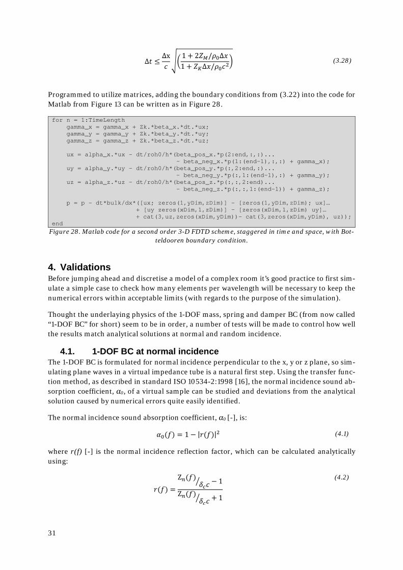
Programmed to utilize matrices, adding the boundary conditions from (3.22) into the code for Matlab from Figure 13 can be written as in Figure 28.

for n = 1:TimeLength gamma_x = gamma_x + Zk.*beta_x.*dt.*ux; gamma_y = gamma_y + Zk.*beta_y.*dt.*uy; gamma_z = gamma_z + Zk.*beta_z.*dt.*uz; ux = alpha_x.*ux - dt/roh0/h*(beta_pos_x.*p(2:end,:,:)... - beta_neg_x.*p(1:(end-1),:,:) + gamma_x); uy = alpha_y.*uy - dt/roh0/h*(beta_pos_y.*p(:,2:end,:)... - beta_neg_y.*p(:,1:(end-1),:) + gamma_y); uz = alpha_z.*uz - dt/roh0/h*(beta_pos_z.*p(:,:,2:end)... - beta_neg_z.*p(:,:,1:(end-1)) + gamma_z); p = p - dt*bulk/dx*([ux; zeros(1,yDim,zDim)] - [zeros(1,yDim,zDim); ux]… + [uy zeros(xDim,1,zDim)] - [zeros(xDim,1,zDim) uy]… + cat(3,uz,zeros(xDim,yDim))- cat(3,zeros(xDim,yDim), uz)); end

Figure 28. Matlab code for a second order 3-D FDTD scheme, staggered in time and space, with Bot-teldooren boundary condition.

4. Validations Before jumping ahead and discretise a model of a complex room it’s good practice to first sim-ulate a simple case to check how many elements per wavelength will be necessary to keep the numerical errors within acceptable limits (with regards to the purpose of the simulation).

Thought the underlaying physics of the 1-DOF mass, spring and damper BC (from now called “1-DOF BC” for short) seem to be in order, a number of tests will be made to control how well the results match analytical solutions at normal and random incidence.

4.1. 1-DOF BC at normal incidence The 1-DOF BC is formulated for normal incidence perpendicular to the x, y or z plane, so sim-ulating plane waves in a virtual impedance tube is a natural first step. Using the transfer func-tion method, as described in standard ISO 10534-2:1998 [16], the normal incidence sound ab-sorption coefficient, α0, of a virtual sample can be studied and deviations from the analytical solution caused by numerical errors quite easily identified.

The normal incidence sound absorption coefficient, α0 [-], is:

𝛼𝛼0(𝑓𝑓) = 1 − |𝑓𝑓(𝑓𝑓)|2

(4.1)

where r(f) [-] is the normal incidence reflection factor, which can be calculated analytically using:

𝑓𝑓(𝑓𝑓) =Z𝑛𝑛(𝑓𝑓)

𝛿𝛿𝑠𝑠𝑐𝑐� − 1

Z𝑛𝑛(𝑓𝑓)𝛿𝛿𝑠𝑠𝑐𝑐� + 1

(4.2)

32

By inserting (4.2) into (4.1) the analytically derived normal incidence sound absorption coeffi-cient, α0, can be calculated:

𝛼𝛼0(𝑓𝑓)𝑚𝑚𝑛𝑛𝑚𝑚𝑒𝑒𝑦𝑦𝑡𝑡𝑖𝑖𝑠𝑠𝑚𝑚𝑒𝑒 = 1 − �Z𝑛𝑛(𝑓𝑓)


Z𝑛𝑛(𝑓𝑓)𝛿𝛿𝑠𝑠𝑐𝑐� + 1

�

2

where Zn is taken from (3.5):

(4.3)

𝑍𝑍𝑛𝑛(𝑓𝑓) = 𝑍𝑍𝑅𝑅 + 𝑖𝑖2𝜋𝜋𝑓𝑓𝑍𝑍𝑀𝑀 + 𝑍𝑍𝐾𝐾𝑖𝑖2𝜋𝜋𝑓𝑓� (4.4)

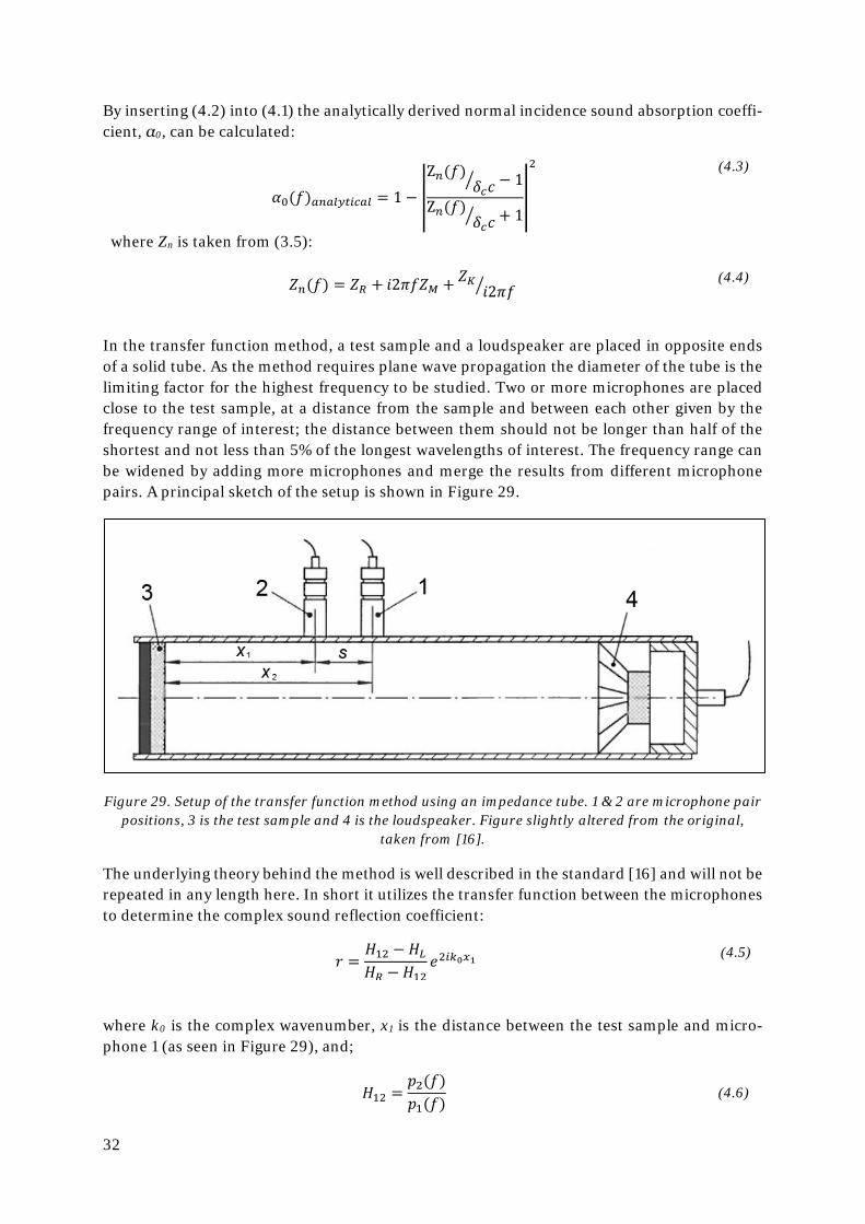
In the transfer function method, a test sample and a loudspeaker are placed in opposite ends of a solid tube. As the method requires plane wave propagation the diameter of the tube is the limiting factor for the highest frequency to be studied. Two or more microphones are placed close to the test sample, at a distance from the sample and between each other given by the frequency range of interest; the distance between them should not be longer than half of the shortest and not less than 5% of the longest wavelengths of interest. The frequency range can be widened by adding more microphones and merge the results from different microphone pairs. A principal sketch of the setup is shown in Figure 29.

Figure 29. Setup of the transfer function method using an impedance tube. 1 & 2 are microphone pair positions, 3 is the test sample and 4 is the loudspeaker. Figure slightly altered from the original,

taken from [16].

The underlying theory behind the method is well described in the standard [16] and will not be repeated in any length here. In short it utilizes the transfer function between the microphones to determine the complex sound reflection coefficient:

𝑓𝑓 =𝐻𝐻12 − 𝐻𝐻𝐿𝐿𝐻𝐻𝑅𝑅 − 𝐻𝐻12

𝑒𝑒2𝑖𝑖𝑘𝑘0𝑥𝑥1 (4.5)

where k0 is the complex wavenumber, x1 is the distance between the test sample and micro-phone 1 (as seen in Figure 29), and;

𝐻𝐻12 =𝑝𝑝2(𝑓𝑓)𝑝𝑝1(𝑓𝑓)

(4.6)

33

𝐻𝐻𝐿𝐿 =𝑝𝑝2𝐿𝐿(𝑓𝑓)𝑝𝑝1𝐿𝐿(𝑓𝑓)

= 𝑒𝑒−𝑖𝑖𝑘𝑘0(𝑥𝑥1−𝑥𝑥2) = 𝑒𝑒−𝑖𝑖𝑘𝑘0𝑡𝑡 (4.7)

𝐻𝐻𝑅𝑅 =𝑝𝑝2𝑅𝑅(𝑓𝑓)𝑝𝑝1𝑅𝑅(𝑓𝑓)

= 𝑒𝑒𝑖𝑖𝑘𝑘0(𝑥𝑥1−𝑥𝑥2) = 𝑒𝑒𝑖𝑖𝑘𝑘0𝑡𝑡 (4.8)

where p1 and p2 [Pa] are the sound pressure measured by the microphone pair and x1, x2 and s [m] distances shown in Figure 29. The normal incidence absorption coefficient, α0, can then be written as a function of frequency as:

𝛼𝛼0(𝑓𝑓) = 1 − |r|2 = 1 − �

𝑝𝑝2(𝑓𝑓)𝑝𝑝1(𝑓𝑓) − 𝑒𝑒−𝑖𝑖2𝜋𝜋𝑠𝑠𝑡𝑡 𝑠𝑠⁄

𝑒𝑒𝑖𝑖2𝜋𝜋𝑠𝑠𝑡𝑡 𝑠𝑠⁄ − 𝑝𝑝2(𝑓𝑓)𝑝𝑝1(𝑓𝑓)

𝑒𝑒𝑡𝑡−𝑖𝑖4𝜋𝜋𝜋𝜋𝑥𝑥1 𝑐𝑐⁄ �

2

(4.9)

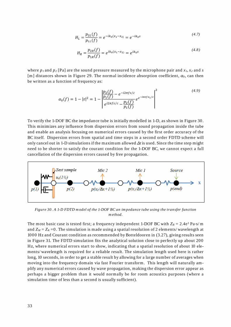
To verify the 1-DOF BC the impedance tube is initially modelled in 1-D, as shown in Figure 30. This minimizes any influence from dispersion errors from sound propagation inside the tube and enable an analysis focusing on numerical errors caused by the first order accuracy of the BC itself. Dispersion errors from spatial and time steps in a second order FDTD scheme will only cancel out in 1-D simulations if the maximum allowed ∆t is used. Since the time step might need to be shorter to satisfy the courant condition for the 1-DOF BC, we cannot expect a full cancellation of the dispersion errors caused by free propagation.

Figure 30. A 1-D FDTD model of the 1-DOF BC an impedance tube using the transfer function method.

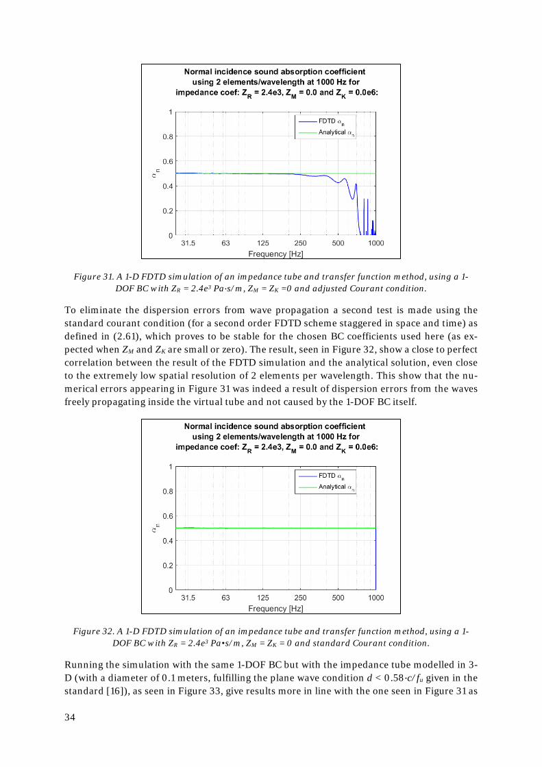
The most basic case is tested first; a frequency independent 1-DOF BC with ZR = 2.4e3 Pa∙s/m and ZM = ZK =0. The simulation is made using a spatial resolution of 2 elements/wavelength at 1000 Hz and Courant condition as recommended by Botteldooren in (3.27), giving results seen in Figure 31. The FDTD simulation fits the analytical solution close to perfectly up about 200 Hz, where numerical errors start to show, indicating that a spatial resolution of about 10 ele-ments/wavelength is required for a reliable result. The simulation length used here is rather long, 10 seconds, in order to get a stable result by allowing for a large number of averages when moving into the frequency domain via fast Fourier transform. This length will naturally am-plify any numerical errors caused by wave propagation, making the dispersion error appear as perhaps a bigger problem than it would normally be for room acoustics purposes (where a simulation time of less than a second is usually sufficient).

34

Figure 31. A 1-D FDTD simulation of an impedance tube and transfer function method, using a 1-DOF BC with ZR = 2.4e3 Pa∙s/m, ZM = ZK =0 and adjusted Courant condition.

To eliminate the dispersion errors from wave propagation a second test is made using the standard courant condition (for a second order FDTD scheme staggered in space and time) as defined in (2.61), which proves to be stable for the chosen BC coefficients used here (as ex-pected when ZM and ZK are small or zero). The result, seen in Figure 32, show a close to perfect correlation between the result of the FDTD simulation and the analytical solution, even close to the extremely low spatial resolution of 2 elements per wavelength. This show that the nu-merical errors appearing in Figure 31 was indeed a result of dispersion errors from the waves freely propagating inside the virtual tube and not caused by the 1-DOF BC itself.

Figure 32. A 1-D FDTD simulation of an impedance tube and transfer function method, using a 1-DOF BC with ZR = 2.4e3 Pa•s/m, ZM = ZK = 0 and standard Courant condition.

Running the simulation with the same 1-DOF BC but with the impedance tube modelled in 3-D (with a diameter of 0.1 meters, fulfilling the plane wave condition d < 0.58∙c/fu given in the standard [16]), as seen in Figure 33, give results more in line with the one seen in Figure 31 as

35

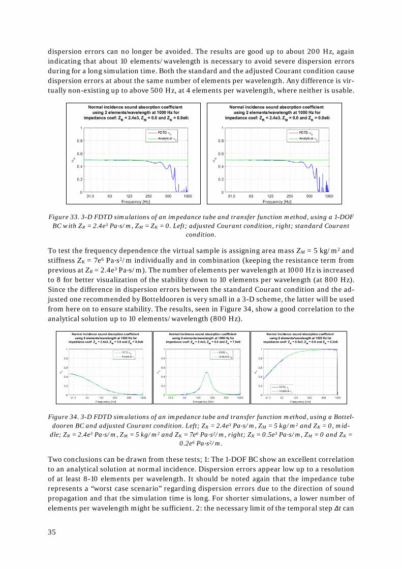
dispersion errors can no longer be avoided. The results are good up to about 200 Hz, again indicating that about 10 elements/wavelength is necessary to avoid severe dispersion errors during for a long simulation time. Both the standard and the adjusted Courant condition cause dispersion errors at about the same number of elements per wavelength. Any difference is vir-tually non-existing up to above 500 Hz, at 4 elements per wavelength, where neither is usable.

Figure 33. 3-D FDTD simulations of an impedance tube and transfer function method, using a 1-DOF BC with ZR = 2.4e3 Pa∙s/m, ZM = ZK = 0. Left; adjusted Courant condition, right; standard Courant

condition.

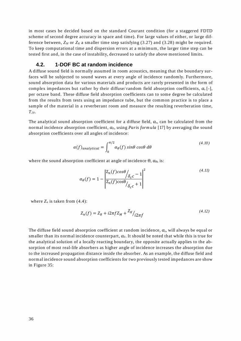
To test the frequency dependence the virtual sample is assigning area mass ZM = 5 kg/m2 and stiffness ZK = 7e6 Pa∙s2/m individually and in combination (keeping the resistance term from previous at ZR = 2.4e3 Pa∙s/m). The number of elements per wavelength at 1000 Hz is increased to 8 for better visualization of the stability down to 10 elements per wavelength (at 800 Hz). Since the difference in dispersion errors between the standard Courant condition and the ad-justed one recommended by Botteldooren is very small in a 3-D scheme, the latter will be used from here on to ensure stability. The results, seen in Figure 34, show a good correlation to the analytical solution up to 10 elements/wavelength (800 Hz).

Figure 34. 3-D FDTD simulations of an impedance tube and transfer function method, using a Bottel-dooren BC and adjusted Courant condition. Left; ZR = 2.4e3 Pa∙s/m, ZM = 5 kg/m2 and ZK = 0, mid-

dle; ZR = 2.4e3 Pa∙s/m, ZM = 5 kg/m2 and ZK = 7e6 Pa∙s2/m, right; ZR = 0.5e3 Pa∙s/m, ZM = 0 and ZK = 0.2e6 Pa∙s2/m.

Two conclusions can be drawn from these tests; 1: The 1-DOF BC show an excellent correlation to an analytical solution at normal incidence. Dispersion errors appear low up to a resolution of at least 8-10 elements per wavelength. It should be noted again that the impedance tube represents a “worst case scenario” regarding dispersion errors due to the direction of sound propagation and that the simulation time is long. For shorter simulations, a lower number of elements per wavelength might be sufficient. 2: the necessary limit of the temporal step ∆t can

36

in most cases be decided based on the standard Courant condition (for a staggered FDTD scheme of second degree accuracy in space and time). For large values of either, or large dif-ference between, ZM or ZK a smaller time step satisfying (3.27) and (3.28) might be required. To keep computational time and dispersion errors at a minimum, the larger time step can be tested first and, in the case of instability, decreased to satisfy the above mentioned limits.

4.2. 1-DOF BC at random incidence A diffuse sound field is normally assumed in room acoustics, meaning that the boundary sur-faces will be subjected to sound waves at every angle of incidence randomly. Furthermore, sound absorption data for various materials and products are rarely presented in the form of complex impedances but rather by their diffuse/random field absorption coefficients, αs [-], per octave band. These diffuse field absorption coefficients can to some degree be calculated from the results from tests using an impedance tube, but the common practice is to place a sample of the material in a reverberant room and measure the resulting reverberation time, T20.

The analytical sound absorption coefficient for a diffuse field, αs, can be calculated from the normal incidence absorption coefficient, α0, using Paris formula [17] by averaging the sound absorption coefficients over all angles of incidence:

𝛼𝛼(𝑓𝑓)𝑚𝑚𝑛𝑛𝑚𝑚𝑒𝑒𝑦𝑦𝑡𝑡𝑖𝑖𝑠𝑠𝑚𝑚𝑒𝑒 = � 𝛼𝛼𝜃𝜃(𝑓𝑓) 𝑠𝑠𝑖𝑖𝑛𝑛𝑠𝑠 𝑐𝑐𝑓𝑓𝑠𝑠𝑠𝑠 𝑑𝑑𝑠𝑠𝜋𝜋/2

0

(4.10)

where the sound absorption coefficient at angle of incidence Ɵ, αƟ, is:

𝛼𝛼𝜃𝜃(𝑓𝑓) = 1 − �Z𝑛𝑛(𝑓𝑓)𝑐𝑐𝑓𝑓𝑠𝑠𝑠𝑠


Z𝑛𝑛(𝑓𝑓)cosθ𝛿𝛿𝑠𝑠𝑐𝑐� + 1

�

2

(4.11)

where Zn is taken from (4.4):

𝑍𝑍𝑛𝑛(𝑓𝑓) = 𝑍𝑍𝑅𝑅 + 𝑖𝑖2𝜋𝜋𝑓𝑓𝑍𝑍𝑀𝑀 + 𝑍𝑍𝐾𝐾𝑖𝑖2𝜋𝜋𝑓𝑓� (4.12)

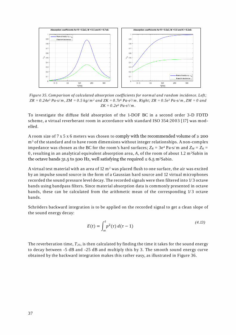
The diffuse field sound absorption coefficient at random incidence, αs, will always be equal or smaller than its normal incidence counterpart, α0. It should be noted that while this is true for the analytical solution of a locally reacting boundary, the opposite actually applies to the ab-sorption of most real-life absorbers as higher angle of incidence increases the absorption due to the increased propagation distance inside the absorber. As an example, the diffuse field and normal incidence sound absorption coefficients for two previously tested impedances are show in Figure 35:

37

Figure 35. Comparison of calculated absorption coefficients for normal and random incidence. Left; ZR = 0.24e3 Pa∙s/m, ZM = 0.5 kg/m2 and ZK = 0.7e6 Pa∙s2/m. Right; ZR = 0.5e3 Pa∙s/m, ZM = 0 and

ZK = 0.2e6 Pa∙s2/m.

To investigate the diffuse field absorption of the 1-DOF BC in a second order 3-D FDTD scheme, a virtual reverberant room in accordance with standard ISO 354:2003 [17] was mod-elled.

A room size of 7 x 5 x 6 meters was chosen to comply with the recommended volume of ≥ 200 m3 of the standard and to have room dimensions without integer relationships. A non-complex impedance was chosen as the BC for the room’s hard surfaces; ZR = 3e4 Pa∙s/m and ZM = ZK = 0, resulting in an analytical equivalent absorption area, A, of the room of about 1.2 m2Sabin in the octave bands 31.5 to 500 Hz, well satisfying the required ≤ 6.5 m2Sabin.

A virtual test material with an area of 12 m2 was placed flush to one surface, the air was excited by an impulse sound source in the form of a Gaussian hard source and 12 virtual microphones recorded the sound pressure level decay. The recorded signals were then filtered into 1/3 octave bands using bandpass filters. Since material absorption data is commonly presented in octave bands, these can be calculated from the arithmetic mean of the corresponding 1/3 octave bands.

Schröders backward integration is to be applied on the recorded signal to get a clean slope of the sound energy decay:

𝐸𝐸(𝜕𝜕) = � 𝑝𝑝2(𝜏𝜏) 𝑑𝑑(𝜏𝜏 − 1)𝑡𝑡

∞

(4.13)

The reverberation time, T20, is then calculated by finding the time it takes for the sound energy to decay between -5 dB and -25 dB and multiply this by 3. The smooth sound energy curve obtained by the backward integration makes this rather easy, as illustrated in Figure 36.

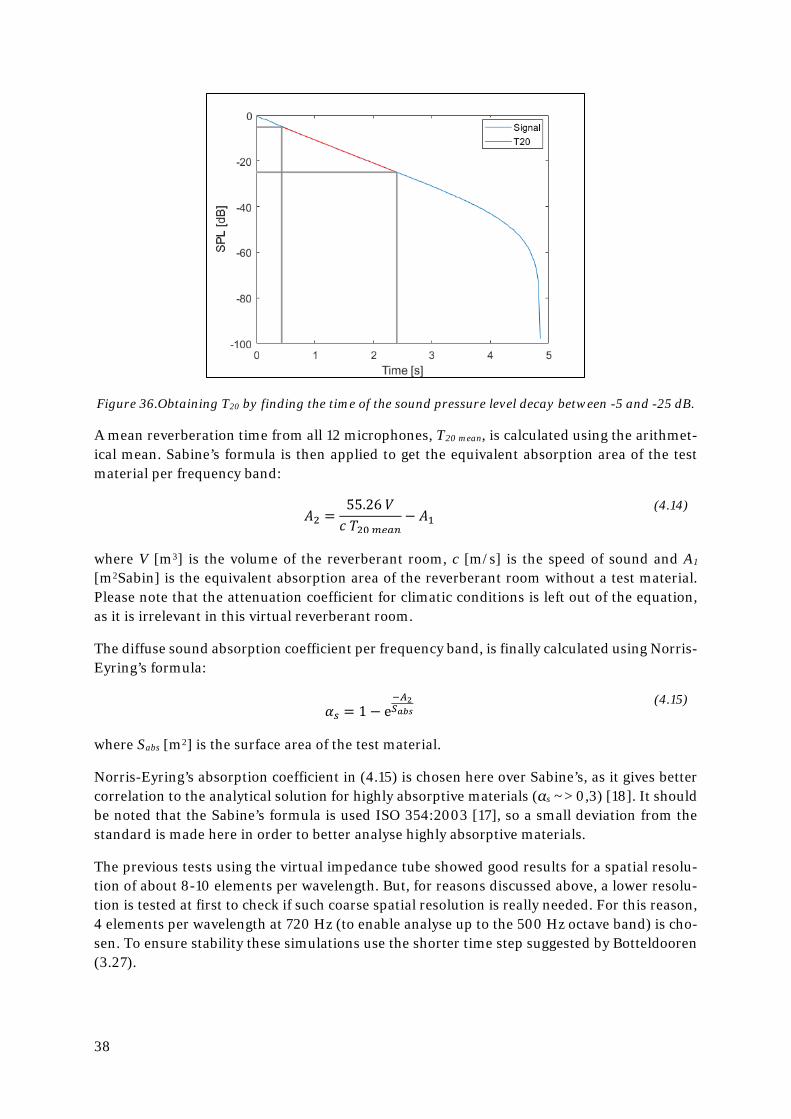
38

Figure 36.Obtaining T20 by finding the time of the sound pressure level decay between -5 and -25 dB.

A mean reverberation time from all 12 microphones, T20 mean, is calculated using the arithmet-ical mean. Sabine’s formula is then applied to get the equivalent absorption area of the test material per frequency band:

𝐴𝐴2 =55.26 𝑉𝑉𝑐𝑐 𝑇𝑇20 𝑡𝑡𝑡𝑡𝑚𝑚𝑛𝑛

− 𝐴𝐴1 (4.14)

where V [m3] is the volume of the reverberant room, c [m/s] is the speed of sound and A1 [m2Sabin] is the equivalent absorption area of the reverberant room without a test material. Please note that the attenuation coefficient for climatic conditions is left out of the equation, as it is irrelevant in this virtual reverberant room.

The diffuse sound absorption coefficient per frequency band, is finally calculated using Norris-Eyring’s formula:

𝛼𝛼𝑡𝑡 = 1 − e−𝐴𝐴2𝑆𝑆𝑎𝑎𝑎𝑎𝑎𝑎

(4.15)

where Sabs [m2] is the surface area of the test material.

Norris-Eyring’s absorption coefficient in (4.15) is chosen here over Sabine’s, as it gives better correlation to the analytical solution for highly absorptive materials (αs ~> 0,3) [18]. It should be noted that the Sabine’s formula is used ISO 354:2003 [17], so a small deviation from the standard is made here in order to better analyse highly absorptive materials.

The previous tests using the virtual impedance tube showed good results for a spatial resolu-tion of about 8-10 elements per wavelength. But, for reasons discussed above, a lower resolu-tion is tested at first to check if such coarse spatial resolution is really needed. For this reason, 4 elements per wavelength at 720 Hz (to enable analyse up to the 500 Hz octave band) is cho-sen. To ensure stability these simulations use the shorter time step suggested by Botteldooren (3.27).

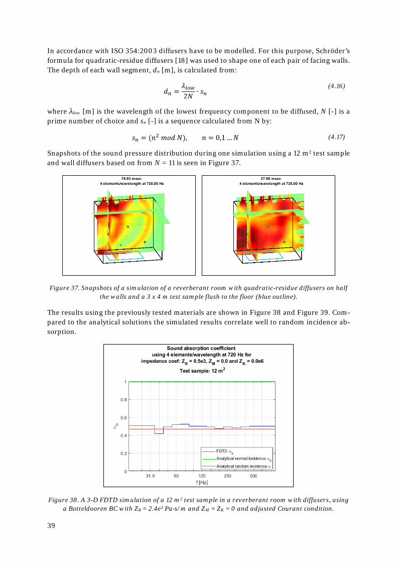
39

In accordance with ISO 354:2003 diffusers have to be modelled. For this purpose, Schröder’s formula for quadratic-residue diffusers [18] was used to shape one of each pair of facing walls. The depth of each wall segment, dn [m], is calculated from:

𝑑𝑑𝑛𝑛 =𝜆𝜆𝑒𝑒𝐸𝐸𝑤𝑤2𝑁𝑁

∙ 𝑠𝑠𝑛𝑛 (4.16)

where λlow [m] is the wavelength of the lowest frequency component to be diffused, N [-] is a prime number of choice and sn [-] is a sequence calculated from N by:

𝑠𝑠𝑛𝑛 = (𝑛𝑛2 𝑚𝑚𝑓𝑓𝑑𝑑 𝑁𝑁), 𝑛𝑛 = 0,1 …𝑁𝑁 (4.17)

Snapshots of the sound pressure distribution during one simulation using a 12 m2 test sample and wall diffusers based on from N = 11 is seen in Figure 37.

Figure 37. Snapshots of a simulation of a reverberant room with quadratic-residue diffusers on half the walls and a 3 x 4 m test sample flush to the floor (blue outline).

The results using the previously tested materials are shown in Figure 38 and Figure 39. Com-pared to the analytical solutions the simulated results correlate well to random incidence ab-sorption.

Figure 38. A 3-D FDTD simulation of a 12 m2 test sample in a reverberant room with diffusers, using a Botteldooren BC with ZR = 2.4e3 Pa∙s/m and ZM = ZK = 0 and adjusted Courant condition.

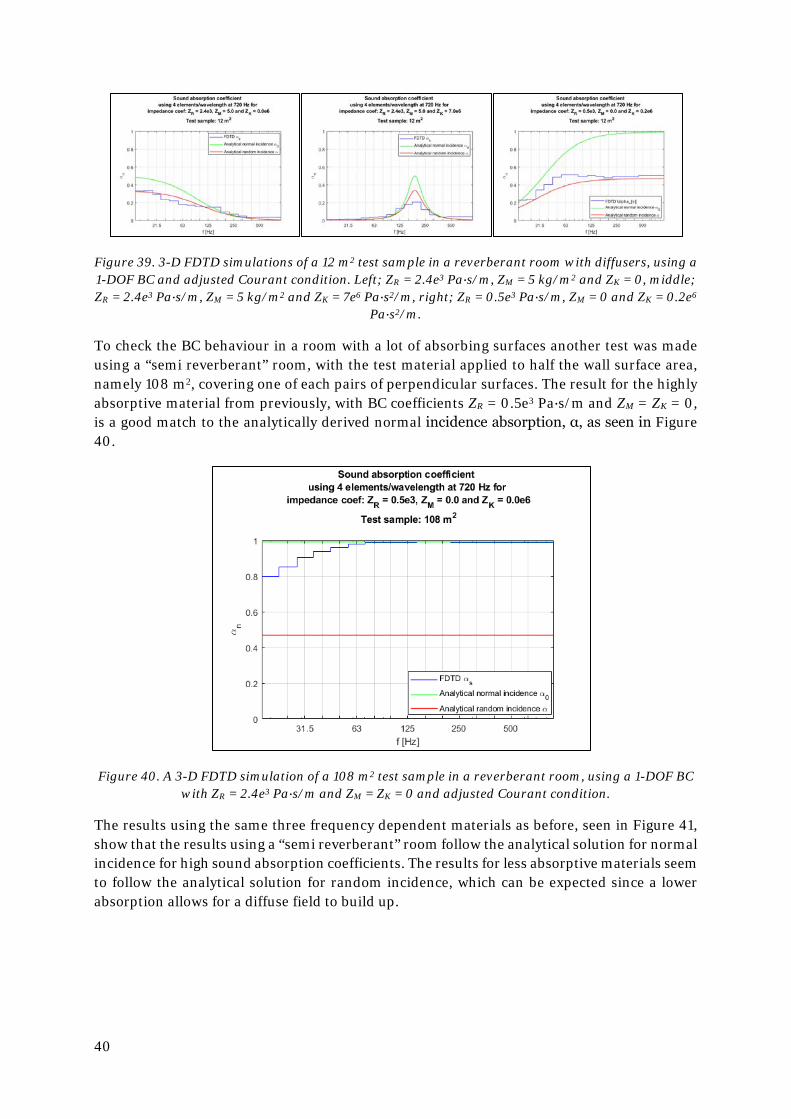
40

Figure 39. 3-D FDTD simulations of a 12 m2 test sample in a reverberant room with diffusers, using a 1-DOF BC and adjusted Courant condition. Left; ZR = 2.4e3 Pa∙s/m, ZM = 5 kg/m2 and ZK = 0, middle; ZR = 2.4e3 Pa∙s/m, ZM = 5 kg/m2 and ZK = 7e6 Pa∙s2/m, right; ZR = 0.5e3 Pa∙s/m, ZM = 0 and ZK = 0.2e6

Pa∙s2/m.

To check the BC behaviour in a room with a lot of absorbing surfaces another test was made using a “semi reverberant” room, with the test material applied to half the wall surface area, namely 108 m2, covering one of each pairs of perpendicular surfaces. The result for the highly absorptive material from previously, with BC coefficients ZR = 0.5e3 Pa∙s/m and ZM = ZK = 0, is a good match to the analytically derived normal incidence absorption, α, as seen in Figure 40.

Figure 40. A 3-D FDTD simulation of a 108 m2 test sample in a reverberant room, using a 1-DOF BC with ZR = 2.4e3 Pa∙s/m and ZM = ZK = 0 and adjusted Courant condition.

The results using the same three frequency dependent materials as before, seen in Figure 41, show that the results using a “semi reverberant” room follow the analytical solution for normal incidence for high sound absorption coefficients. The results for less absorptive materials seem to follow the analytical solution for random incidence, which can be expected since a lower absorption allows for a diffuse field to build up.

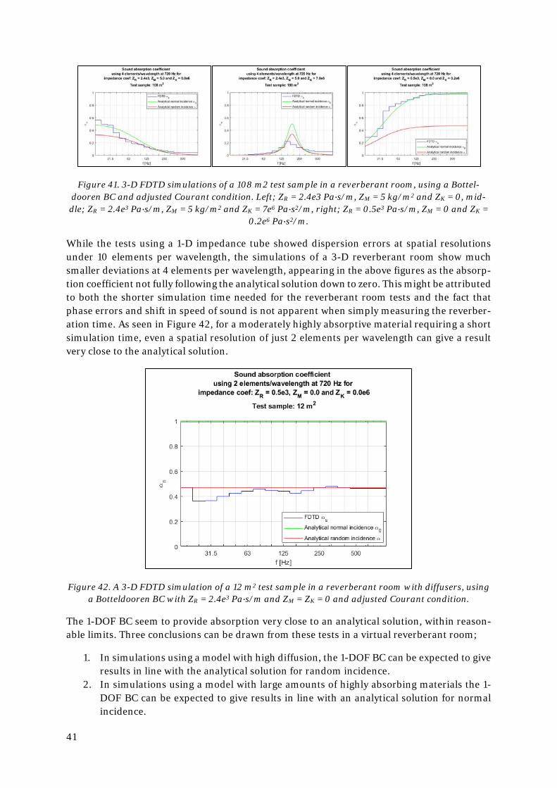
41

Figure 41. 3-D FDTD simulations of a 108 m2 test sample in a reverberant room, using a Bottel-dooren BC and adjusted Courant condition. Left; ZR = 2.4e3 Pa∙s/m, ZM = 5 kg/m2 and ZK = 0, mid-

dle; ZR = 2.4e3 Pa∙s/m, ZM = 5 kg/m2 and ZK = 7e6 Pa∙s2/m, right; ZR = 0.5e3 Pa∙s/m, ZM = 0 and ZK = 0.2e6 Pa∙s2/m.

While the tests using a 1-D impedance tube showed dispersion errors at spatial resolutions under 10 elements per wavelength, the simulations of a 3-D reverberant room show much smaller deviations at 4 elements per wavelength, appearing in the above figures as the absorp-tion coefficient not fully following the analytical solution down to zero. This might be attributed to both the shorter simulation time needed for the reverberant room tests and the fact that phase errors and shift in speed of sound is not apparent when simply measuring the reverber-ation time. As seen in Figure 42, for a moderately highly absorptive material requiring a short simulation time, even a spatial resolution of just 2 elements per wavelength can give a result very close to the analytical solution.

Figure 42. A 3-D FDTD simulation of a 12 m2 test sample in a reverberant room with diffusers, using a Botteldooren BC with ZR = 2.4e3 Pa∙s/m and ZM = ZK = 0 and adjusted Courant condition.

The 1-DOF BC seem to provide absorption very close to an analytical solution, within reason-able limits. Three conclusions can be drawn from these tests in a virtual reverberant room;

1. In simulations using a model with high diffusion, the 1-DOF BC can be expected to give results in line with the analytical solution for random incidence.

2. In simulations using a model with large amounts of highly absorbing materials the 1-DOF BC can be expected to give results in line with an analytical solution for normal incidence.

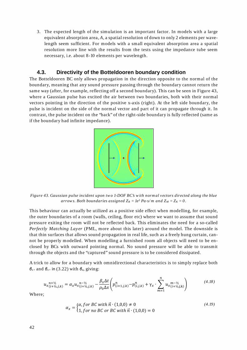
42

3. The expected length of the simulation is an important factor. In models with a large equivalent absorption area, A, a spatial resolution of down to only 2 elements per wave-length seem sufficient. For models with a small equivalent absorption area a spatial resolution more line with the results from the tests using the impedance tube seem necessary, i.e. about 8-10 elements per wavelength.

4.3. Directivity of the Botteldooren boundary condition The Botteldooren BC only allows propagation in the direction opposite to the normal of the boundary, meaning that any sound pressure passing through the boundary cannot return the same way (after, for example, reflecting off a second boundary). This can be seen in Figure 43, where a Gaussian pulse has excited the air between two boundaries, both with their normal vectors pointing in the direction of the positive x-axis (right). At the left side boundary, the pulse is incident on the side of the normal vector and part of it can propagate through it. In contrast, the pulse incident on the “back” of the right-side boundary is fully reflected (same as if the boundary had infinite impedance).

Figure 43. Gaussian pulse incident upon two 1-DOF BC’s with normal vectors directed along the blue arrows. Both boundaries assigned ZR = 1e3 Pa∙s/m and ZM = ZK = 0.

This behaviour can actually be utilized as a positive side effect when modelling, for example, the outer boundaries of a room (walls, ceiling, floor etc) where we want to assume that sound pressure exiting the room will not be reflected back. This eliminates the need for a so-called Perfectly Matching Layer (PML, more about this later) around the model. The downside is that thin surfaces that allows sound propagation in real life, such as a freely hung curtain, can-not be properly modelled. When modelling a furnished room all objects will need to be en-closed by BCs with outward pointing normal. No sound pressure will be able to transmit through the objects and the “captured” sound pressure is to be considered dissipated.

A trick to allow for a boundary with omnidirectional characteristics is to simply replace both βx+ and βx+ in (3.22) with βx, giving:

𝑢𝑢𝑥𝑥(𝑖𝑖+½,𝑗𝑗,𝑘𝑘)𝑛𝑛+½ = 𝛼𝛼𝑥𝑥𝑢𝑢𝑥𝑥(𝑖𝑖+½,𝑗𝑗,𝑘𝑘)

𝑛𝑛−½ −𝛽𝛽𝑥𝑥∆𝜕𝜕𝜌𝜌0∆𝜕𝜕

�𝑝𝑝(𝑖𝑖+1,𝑗𝑗,𝑘𝑘)𝑛𝑛 −𝑝𝑝(𝑖𝑖,𝑗𝑗,𝑘𝑘)

𝑛𝑛 + γ𝑥𝑥 ∙ � 𝑢𝑢𝑥𝑥(𝑖𝑖+½,j,k)𝑡𝑡−½

𝑛𝑛

𝑡𝑡=1

� (4.18)

Where;

𝛼𝛼𝑥𝑥 = �𝛼𝛼, 𝑓𝑓𝑓𝑓𝑓𝑓 𝐵𝐵𝐶𝐶 𝑤𝑤𝑖𝑖𝜕𝜕ℎ 𝑛𝑛�⃗ ∙ (1,0,0) ≠ 0 1,𝑓𝑓𝑓𝑓𝑓𝑓 𝑛𝑛𝑓𝑓 𝐵𝐵𝐶𝐶 𝑓𝑓𝑓𝑓 𝐵𝐵𝐶𝐶 𝑤𝑤𝑖𝑖𝜕𝜕ℎ 𝑛𝑛�⃗ ∙ (1,0,0) = 0

(4.19)

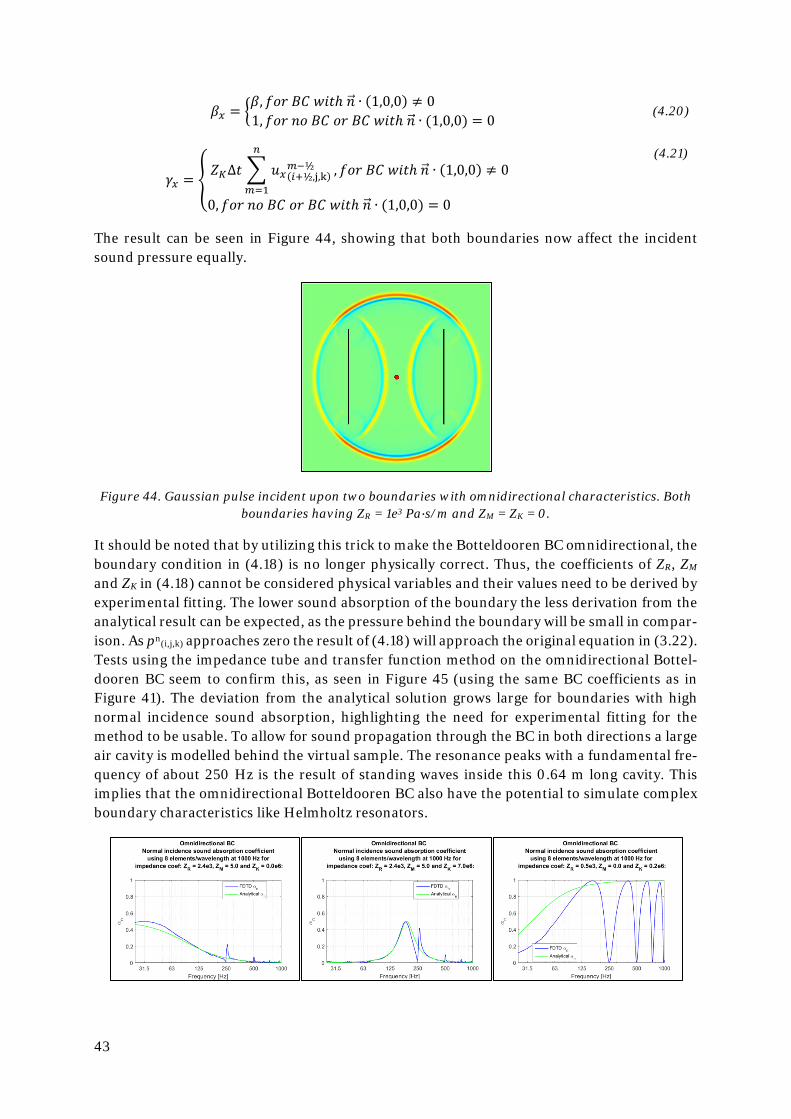
43

𝛽𝛽𝑥𝑥 = �𝛽𝛽,𝑓𝑓𝑓𝑓𝑓𝑓 𝐵𝐵𝐶𝐶 𝑤𝑤𝑖𝑖𝜕𝜕ℎ 𝑛𝑛�⃗ ∙ (1,0,0) ≠ 0 1,𝑓𝑓𝑓𝑓𝑓𝑓 𝑛𝑛𝑓𝑓 𝐵𝐵𝐶𝐶 𝑓𝑓𝑓𝑓 𝐵𝐵𝐶𝐶 𝑤𝑤𝑖𝑖𝜕𝜕ℎ 𝑛𝑛�⃗ ∙ (1,0,0) = 0

(4.20)

𝛾𝛾𝑥𝑥 = �𝑍𝑍𝐾𝐾∆𝜕𝜕 � 𝑢𝑢𝑥𝑥(𝑖𝑖+½,j,k)

𝑡𝑡−½𝑛𝑛

𝑡𝑡=1

,𝑓𝑓𝑓𝑓𝑓𝑓 𝐵𝐵𝐶𝐶 𝑤𝑤𝑖𝑖𝜕𝜕ℎ 𝑛𝑛�⃗ ∙ (1,0,0) ≠ 0

0,𝑓𝑓𝑓𝑓𝑓𝑓 𝑛𝑛𝑓𝑓 𝐵𝐵𝐶𝐶 𝑓𝑓𝑓𝑓 𝐵𝐵𝐶𝐶 𝑤𝑤𝑖𝑖𝜕𝜕ℎ 𝑛𝑛�⃗ ∙ (1,0,0) = 0

(4.21)

The result can be seen in Figure 44, showing that both boundaries now affect the incident sound pressure equally.

Figure 44. Gaussian pulse incident upon two boundaries with omnidirectional characteristics. Both boundaries having ZR = 1e3 Pa∙s/m and ZM = ZK = 0.

It should be noted that by utilizing this trick to make the Botteldooren BC omnidirectional, the boundary condition in (4.18) is no longer physically correct. Thus, the coefficients of ZR, ZM and ZK in (4.18) cannot be considered physical variables and their values need to be derived by experimental fitting. The lower sound absorption of the boundary the less derivation from the analytical result can be expected, as the pressure behind the boundary will be small in compar-ison. As pn(i,j,k) approaches zero the result of (4.18) will approach the original equation in (3.22). Tests using the impedance tube and transfer function method on the omnidirectional Bottel-dooren BC seem to confirm this, as seen in Figure 45 (using the same BC coefficients as in Figure 41). The deviation from the analytical solution grows large for boundaries with high normal incidence sound absorption, highlighting the need for experimental fitting for the method to be usable. To allow for sound propagation through the BC in both directions a large air cavity is modelled behind the virtual sample. The resonance peaks with a fundamental fre-quency of about 250 Hz is the result of standing waves inside this 0.64 m long cavity. This implies that the omnidirectional Botteldooren BC also have the potential to simulate complex boundary characteristics like Helmholtz resonators.

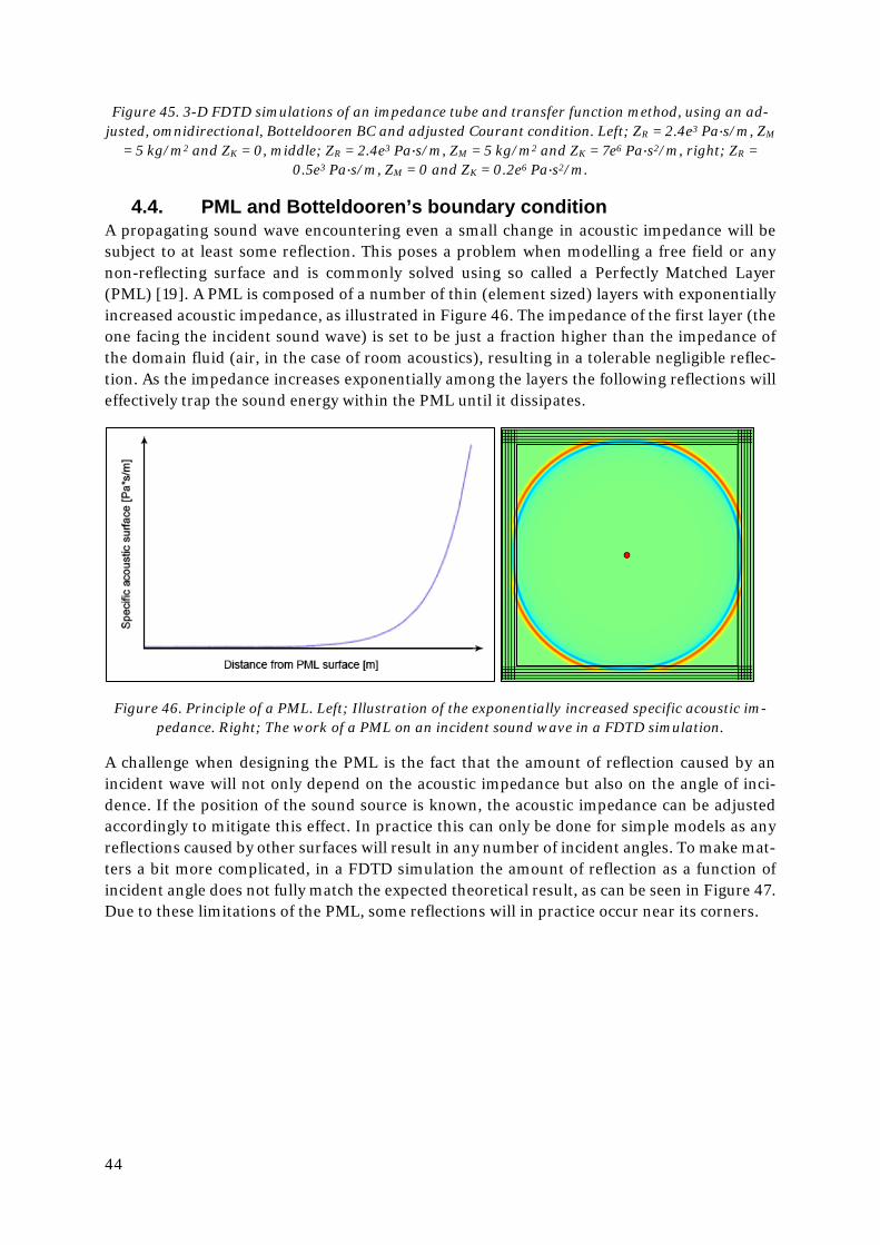
44

Figure 45. 3-D FDTD simulations of an impedance tube and transfer function method, using an ad-justed, omnidirectional, Botteldooren BC and adjusted Courant condition. Left; ZR = 2.4e3 Pa∙s/m, ZM

= 5 kg/m2 and ZK = 0, middle; ZR = 2.4e3 Pa∙s/m, ZM = 5 kg/m2 and ZK = 7e6 Pa∙s2/m, right; ZR = 0.5e3 Pa∙s/m, ZM = 0 and ZK = 0.2e6 Pa∙s2/m.

4.4. PML and Botteldooren’s boundary condition A propagating sound wave encountering even a small change in acoustic impedance will be subject to at least some reflection. This poses a problem when modelling a free field or any non-reflecting surface and is commonly solved using so called a Perfectly Matched Layer (PML) [19]. A PML is composed of a number of thin (element sized) layers with exponentially increased acoustic impedance, as illustrated in Figure 46. The impedance of the first layer (the one facing the incident sound wave) is set to be just a fraction higher than the impedance of the domain fluid (air, in the case of room acoustics), resulting in a tolerable negligible reflec-tion. As the impedance increases exponentially among the layers the following reflections will effectively trap the sound energy within the PML until it dissipates.

Figure 46. Principle of a PML. Left; Illustration of the exponentially increased specific acoustic im-pedance. Right; The work of a PML on an incident sound wave in a FDTD simulation.

A challenge when designing the PML is the fact that the amount of reflection caused by an incident wave will not only depend on the acoustic impedance but also on the angle of inci-dence. If the position of the sound source is known, the acoustic impedance can be adjusted accordingly to mitigate this effect. In practice this can only be done for simple models as any reflections caused by other surfaces will result in any number of incident angles. To make mat-ters a bit more complicated, in a FDTD simulation the amount of reflection as a function of incident angle does not fully match the expected theoretical result, as can be seen in Figure 47. Due to these limitations of the PML, some reflections will in practice occur near its corners.

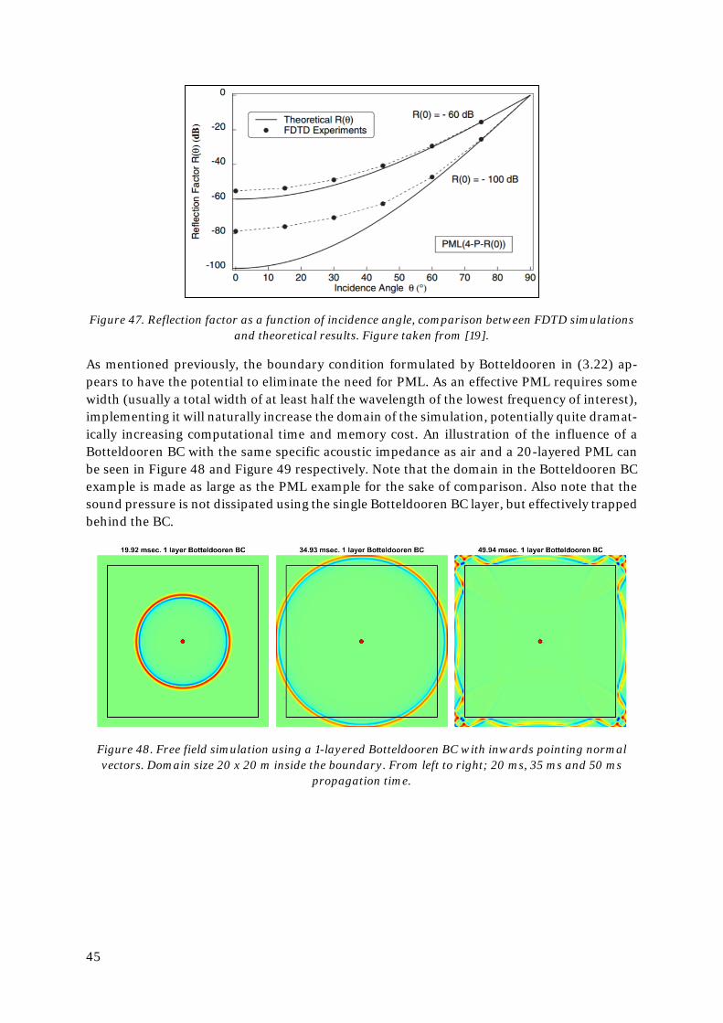
45

Figure 47. Reflection factor as a function of incidence angle, comparison between FDTD simulations and theoretical results. Figure taken from [19].

As mentioned previously, the boundary condition formulated by Botteldooren in (3.22) ap-pears to have the potential to eliminate the need for PML. As an effective PML requires some width (usually a total width of at least half the wavelength of the lowest frequency of interest), implementing it will naturally increase the domain of the simulation, potentially quite dramat-ically increasing computational time and memory cost. An illustration of the influence of a Botteldooren BC with the same specific acoustic impedance as air and a 20-layered PML can be seen in Figure 48 and Figure 49 respectively. Note that the domain in the Botteldooren BC example is made as large as the PML example for the sake of comparison. Also note that the sound pressure is not dissipated using the single Botteldooren BC layer, but effectively trapped behind the BC.

Figure 48. Free field simulation using a 1-layered Botteldooren BC with inwards pointing normal vectors. Domain size 20 x 20 m inside the boundary. From left to right; 20 ms, 35 ms and 50 ms

propagation time.

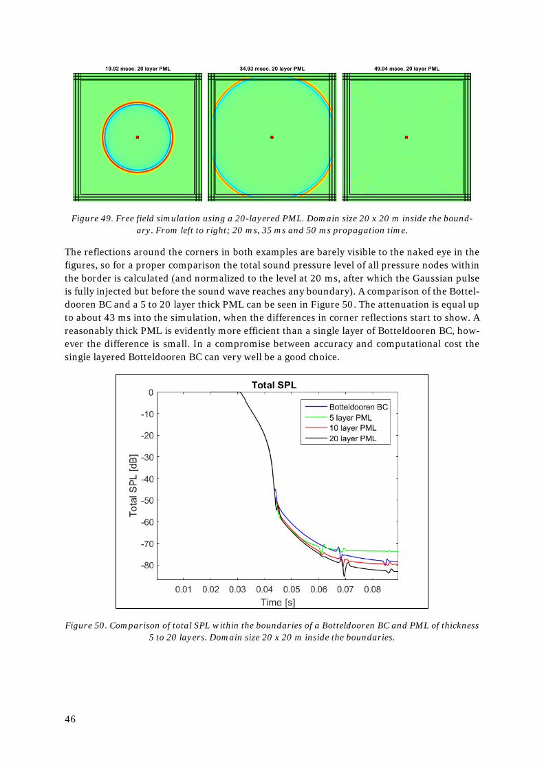
46

Figure 49. Free field simulation using a 20-layered PML. Domain size 20 x 20 m inside the bound-ary. From left to right; 20 ms, 35 ms and 50 ms propagation time.

The reflections around the corners in both examples are barely visible to the naked eye in the figures, so for a proper comparison the total sound pressure level of all pressure nodes within the border is calculated (and normalized to the level at 20 ms, after which the Gaussian pulse is fully injected but before the sound wave reaches any boundary). A comparison of the Bottel-dooren BC and a 5 to 20 layer thick PML can be seen in Figure 50. The attenuation is equal up to about 43 ms into the simulation, when the differences in corner reflections start to show. A reasonably thick PML is evidently more efficient than a single layer of Botteldooren BC, how-ever the difference is small. In a compromise between accuracy and computational cost the single layered Botteldooren BC can very well be a good choice.

Figure 50. Comparison of total SPL within the boundaries of a Botteldooren BC and PML of thickness 5 to 20 layers. Domain size 20 x 20 m inside the boundaries.

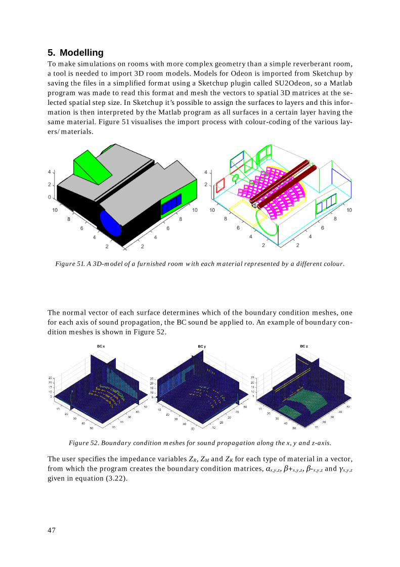
47

5. Modelling To make simulations on rooms with more complex geometry than a simple reverberant room, a tool is needed to import 3D room models. Models for Odeon is imported from Sketchup by saving the files in a simplified format using a Sketchup plugin called SU2Odeon, so a Matlab program was made to read this format and mesh the vectors to spatial 3D matrices at the se-lected spatial step size. In Sketchup it’s possible to assign the surfaces to layers and this infor-mation is then interpreted by the Matlab program as all surfaces in a certain layer having the same material. Figure 51 visualises the import process with colour-coding of the various lay-ers/materials.

Figure 51. A 3D-model of a furnished room with each material represented by a different colour.

The normal vector of each surface determines which of the boundary condition meshes, one for each axis of sound propagation, the BC sound be applied to. An example of boundary con-dition meshes is shown in Figure 52.

Figure 52. Boundary condition meshes for sound propagation along the x, y and z-axis.

The user specifies the impedance variables ZR, ZM and ZK for each type of material in a vector, from which the program creates the boundary condition matrices, αx,y,z, β+x,y,z, β-x,y,z and γx,y,z given in equation (3.22).

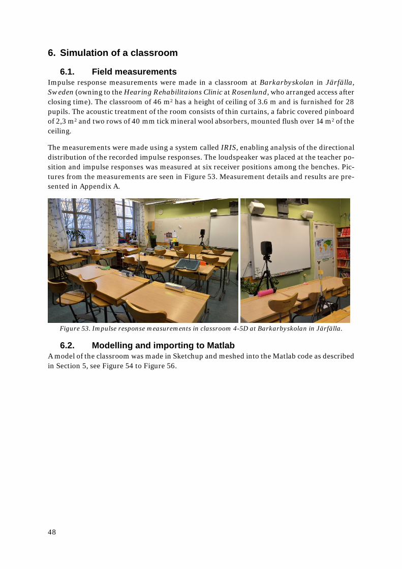
48

6. Simulation of a classroom

6.1. Field measurements Impulse response measurements were made in a classroom at Barkarbyskolan in Järfälla, Sweden (owning to the Hearing Rehabilitaions Clinic at Rosenlund, who arranged access after closing time). The classroom of 46 m2 has a height of ceiling of 3.6 m and is furnished for 28 pupils. The acoustic treatment of the room consists of thin curtains, a fabric covered pinboard of 2,3 m2 and two rows of 40 mm tick mineral wool absorbers, mounted flush over 14 m2 of the ceiling.

The measurements were made using a system called IRIS, enabling analysis of the directional distribution of the recorded impulse responses. The loudspeaker was placed at the teacher po-sition and impulse responses was measured at six receiver positions among the benches. Pic-tures from the measurements are seen in Figure 53. Measurement details and results are pre-sented in Appendix A.

Figure 53. Impulse response measurements in classroom 4-5D at Barkarbyskolan in Järfälla.

6.2. Modelling and importing to Matlab A model of the classroom was made in Sketchup and meshed into the Matlab code as described in Section 5, see Figure 54 to Figure 56.

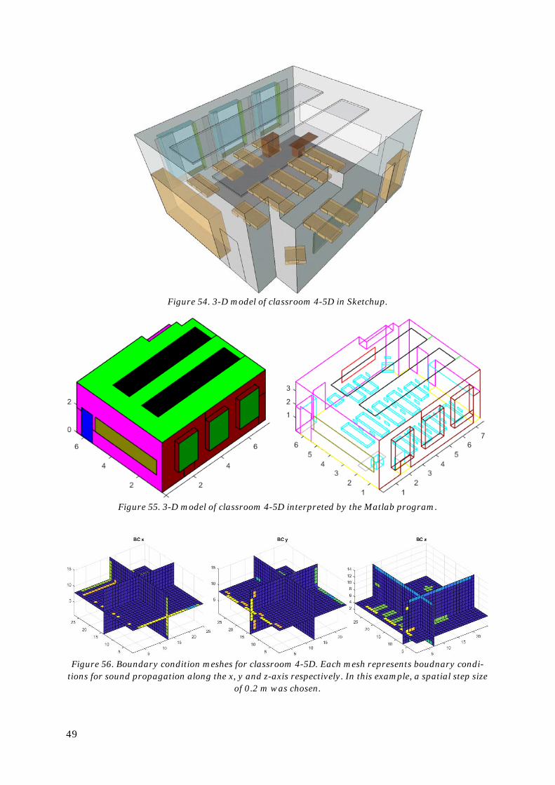
49

Figure 54. 3-D model of classroom 4-5D in Sketchup.

Figure 55. 3-D model of classroom 4-5D interpreted by the Matlab program.

Figure 56. Boundary condition meshes for classroom 4-5D. Each mesh represents boudnary condi-

tions for sound propagation along the x, y and z-axis respectively. In this example, a spatial step size of 0.2 m was chosen.

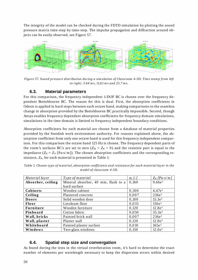
50

The integrity of the model can be checked during the FDTD simulation by plotting the sound pressure matrix time-step by time-step. The impulse propagation and diffraction around ob-jects can be easily observed, see Figure 57.

Figure 57. Sound pressure distribution during a simulation of Classroom 4-5D. Time stamp from left to right; 3.64 ms, 11,61 ms and 25.7 ms.

6.3. Material parameters For this comparison, the frequency independent 1-DOF BC is chosen over the frequency de-pendent Botteldooren BC. The reason for this is dual. First, the absorption coefficients in Odeon is applied in hard steps between each octave band, making comparisons to the seamless change in absorption provided by the Botteldooren BC practically impossible. Second, though Ansys enables frequency dependent absorption coefficients for frequency domain simulations, simulations in the time domain is limited to frequency independent boundary conditions.

Absorption coefficients for each material are chosen from a database of material properties provided by the Swedish work environment authority. For reasons explained above, the ab-sorption coefficient from only one octave band is used for this frequency independent compar-ison. For this comparison the octave band 125 Hz is chosen. The frequency dependent parts of the room’s surfaces BC’s are set to zero (ZM = ZK = 0) and the resistive part is equal to the impedance (ZR = ZN [Pa∙s/m]). The chosen absorption coefficients and the corresponding re-sistance, ZR, for each material is presented in Table 1:

Table 1. Chosen type of material, absorption coefficients and resistance for each material layer in the model of classroom 4-5D.

Material layer Type of material αs [-] ZR [Pa∙s/m] Absorber, ceiling Mineral absorber, 40 mm, flush to a

hard surface 0,160 9.66e3

Cabinets Wooden cabinet 0,300 4.47e3 Ceiling Plastered concrete 0,007 236e3 Doors Solid wooden door 0,100 15.3e3 Floor Linoleum floor 0,035 150e3 Furniture Wooden furniture 0,120 12.8e3 Pinboard Cotton fabric 0,050 35.3e3 Wall, bricks Painted brick wall 0,007 236e3 Wall, plaster Plaster wall 0,120 12.8e3 Whiteboard Painted plaster surface 0,010 165e3 Windows Two-glass windows 0,150 12.0e3

6.4. Spatial step size and convergation As found during the tests in the virtual reverberation room, it’s hard to determine the exact number of elements per wavelength necessary to keep the dispersion errors within desired

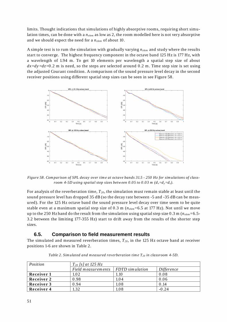
51

limits. Thought indications that simulations of highly absorptive rooms, requiring short simu-lation times, can be done with a nelem as low as 2, the room modelled here is not very absorptive and we should expect the need for a nelem of about 10.

A simple test is to rum the simulation with gradually varying nelem and study where the results start to converge. The highest frequency component in the octave band 125 Hz is 177 Hz, with a wavelength of 1.94 m. To get 10 elements per wavelength a spatial step size of about dx=dy=dz=0.2 m is need, so the steps are selected around 0.2 m. Time step size is set using the adjusted Courant condition. A comparison of the sound pressure level decay in the second receiver positions using different spatial step sizes can be seen in see Figure 58.

Figure 58. Comparison of SPL decay over time at octave bands 31.5 - 250 Hz for simulations of class-room 4-5D using spatial step sizes between 0.05 to 0.03 m (dx=dy=dz).

For analysis of the reverberation time, T20, the simulation must remain stable at least until the sound pressure level has dropped 35 dB (so the decay rate between -5 and -35 dB can be meas-ured). For the 125 Hz octave band the sound pressure level decay over time seem to be quite stable even at a maximum spatial step size of 0.3 m (nelem=6.5 at 177 Hz). Not until we move up to the 250 Hz band do the result from the simulation using spatial step size 0.3 m (nelem=6.5-3.2 between the limiting 177-355 Hz) start to drift away from the results of the shorter step sizes.

6.5. Comparison to field measurement results The simulated and measured reverberation times, T20, in the 125 Hz octave band at receiver positions 1-6 are shown in Table 2.

Table 2. Simulated and measured reverberation time T20 in classroom 4-5D.

Position T20 [s] at 125 Hz Field measurements FDTD simulation Difference

Receiver 1 1.02 1.10 0.08 Receiver 2 0.98 1.04 0.06 Receiver 3 0.94 1.08 0.14 Receiver 4 1.32 1.08 -0.24

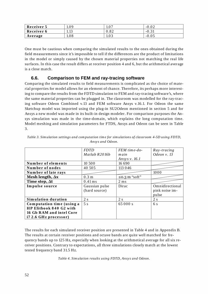
52

Receiver 5 1.09 1.07 -0.02 Receiver 6 1.13 0.82 -0.31 Average 1.08 1.03 -0.05

One must be cautious when comparing the simulated results to the ones obtained during the field measurements since it’s impossible to tell if the differences are the product of limitations in the model or simply caused by the chosen material properties not matching the real life surfaces. In this case the result differs at receiver position 4 and 6, but the arithmetical average is a close match.

6.6. Comparison to FEM and ray-tracing software Comparing the simulated results to field measurements is complicated as the choice of mate-rial properties for model allows for an element of chance. Therefore, its perhaps more interest-ing to compare the results from the FDTD simulation to FEM and ray-tracing software’s, where the same material properties can be plugged in. The classroom was modelled for the ray-trac-ing software Odeon Combined v.13 and FEM software Ansys v.16.1. For Odeon the same Sketchup model was imported using the plug-in SU2Odeon mentioned in section 5 and for Ansys a new model was made in its built-in design modeler. For comparison purposes the An-sys simulation was made in the time-domain, which explains the long computation time. Model meshing and simulation parameters for FTDS, Ansys and Odeon can be seen in Table 3.

Table 3. Simulation settings and computation time for simulations of classroom 4-5D using FDTD, Ansys and Odeon.

FDTD Matlab R2016b

FEM time-do-main Ansys v. 16.1

Ray-tracing Odeon v. 13

Number of elements 10 500 16 690 Number of nodes 40 505 113 046 Number of late rays 1000 Mesh length, ∆x 0.3 m ≤0.3 m “soft” Time step, ∆t 0.41 ms 2 ms Impulse source Gaussian pulse

(hard source) Dirac Omnidirectional

pink noise im-pulse

Simulation duration 2 s 2 s 2 s Computation time (using a HP Elitbook 840 G2 with 16 Gb RAM and intel Core i7 2.6 GHz processor)

5 s 65 000 s 6 s

The results for each simulated receiver position are presented in Table 4 and in Appendix B. The results at certain receiver positions and octave bands are quite well matched for fre-quency bands up to 125 Hz, especially when looking at the arithmetical average for all six re-ceiver positions. Contrary to expectations, all three simulations closely match at the lowest tested frequency band 31.5 Hz.

Table 4. Simulation results using FDTD, Ansys and Odeon.

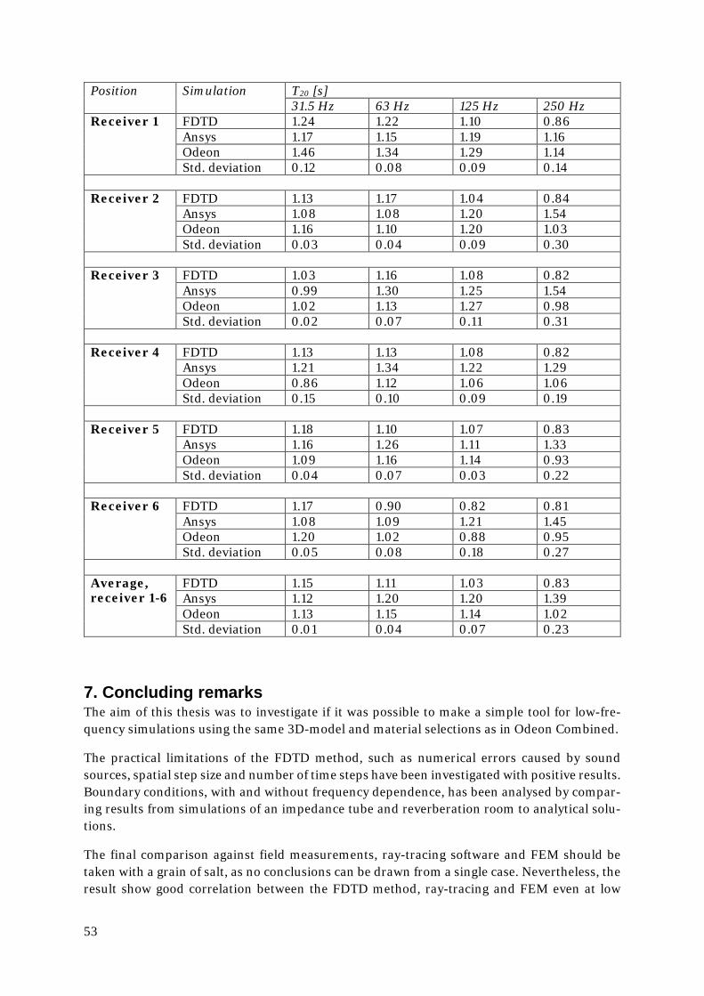
53

Position Simulation T20 [s] 31.5 Hz 63 Hz 125 Hz 250 Hz

Receiver 1 FDTD 1.24 1.22 1.10 0.86 Ansys 1.17 1.15 1.19 1.16 Odeon 1.46 1.34 1.29 1.14 Std. deviation 0.12 0.08 0.09 0.14

Receiver 2 FDTD 1.13 1.17 1.04 0.84

Ansys 1.08 1.08 1.20 1.54 Odeon 1.16 1.10 1.20 1.03 Std. deviation 0.03 0.04 0.09 0.30

Receiver 3 FDTD 1.03 1.16 1.08 0.82


Receiver 4 FDTD 1.13 1.13 1.08 0.82


Receiver 5 FDTD 1.18 1.10 1.07 0.83


Receiver 6 FDTD 1.17 0.90 0.82 0.81


Average, receiver 1-6

FDTD 1.15 1.11 1.03 0.83 Ansys 1.12 1.20 1.20 1.39 Odeon 1.13 1.15 1.14 1.02 Std. deviation 0.01 0.04 0.07 0.23

7. Concluding remarks The aim of this thesis was to investigate if it was possible to make a simple tool for low-fre-quency simulations using the same 3D-model and material selections as in Odeon Combined.

The practical limitations of the FDTD method, such as numerical errors caused by sound sources, spatial step size and number of time steps have been investigated with positive results. Boundary conditions, with and without frequency dependence, has been analysed by compar-ing results from simulations of an impedance tube and reverberation room to analytical solu-tions.

The final comparison against field measurements, ray-tracing software and FEM should be taken with a grain of salt, as no conclusions can be drawn from a single case. Nevertheless, the result show good correlation between the FDTD method, ray-tracing and FEM even at low

54

frequencies down to the 31.5 Hz octave band. This is both good and bad news for the viability of a FDTD tool; the upside is that is seem as accurate as FEM, the downside is that there is no real use for it if ray-tracing in Odeon Combined already cover the behaviour of such low fre-quencies correctly. Opportunities for the use of the FDTD tool might still open for more com-plex models where edge diffraction becomes a more important factor, or simply as a means for a “second opinion”.

The deviations Acad has experienced between simulated results and field measurements might be in part caused by limitations in the ray-tracing software used, but also in part caused by uncertainties in the sound absorption data used for low frequencies. The fact that the results from FDTD and FEM simulations came very close to the results from ray-tracing simulations in low frequencies in the case study indicate the latter.

55

7. References

[1] K. Yee, Numerical solution of initial boundary value problems involving Maxwell's equations in isotropic media, IEEE Transactions on Antennas and Propagation, 1966.

[2] D. Botteldooren, Acoustical finite-difference time-domain simulation in a quasi-Cartesian grid, Laboratory for Electromagnetism and Acoustics, University of Gent, Belgium, 1993.

[3] H. P. Wallin, H. Bodén, U. Carlsson, M. Åbom and R. Glav, Sound and Vibration, KTH Aeronautical and Vehicle engineering, 2014.

[4] S. Marburg, Computational Acoustics of Noise Propagation in Fluids –Finite and Boundary Element Methods, Springer, 2008.

[5] D. M. Sullivan, Electromagnetic simulation using the FDTD method, John Wiley & Sons, 2013.

[6] S. D. Gedney, Introduction to the FDTD Method for Electromagnetics, Morgan & Claypool, 2010.

[7] J. van Mourik and D. Murphy, Explicit Higher-Order FDTD Schemes for 3D Room Acoustic Simulations, IEEE/ACM transactions on audio, speech and language processing, 2014.

[8] J. B. Schneider, Understanding the FDTD method, School of Electrical Engineering and Computer Science, Washington State University, USA, 2010.

[9] J. B. Schneider, C. L. Wagner and O. Ramahi, Implementation of Transparent Sources in FDTD Simulations, IEEE Transactions on antennas and propagation, 1998.

[10] D. Botteldooren, Finite-difference time-domain simulation of low-frequency room acoustic problems, Department of Information Technology, Acoustics Group, University of Gent, Belgium, 1995.

[11] D. M. Sullivan, Frequency-Dependent FDTD Methods Using Z Transforms, IEEE Transactions on antennas and propagation, 1992.

[12] H. Jeong and Y. W. Lam, FDTD modelling of frequency dependent boundary conditions for room acoustics, Acoustics research Centre, University of Salford, UK., 2010.

[13] H. Suzuki, A. Omoto and K. Fujiwara, Treatment of boundary conditions by finite difference time domain method, Acoustic Science and Tech, 2007.

[14] S. Sakamoto, H. Nagatomo, A. Ushiyama and H. Tachibana, Calculation of impulse responses and acoustic parameters in a hall by the finite-difference time-domain method, Acoustic Science and Tech, 2008.

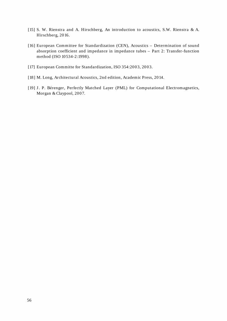
56

[15] S. W. Rienstra and A. Hirschberg, An introduction to acoustics, S.W. Rienstra & A. Hirschberg, 2016.

[16] European Committee for Standardization (CEN), Acoustics – Determination of sound absorption coefficient and impedance in impedance tubes – Part 2: Transfer-function method (ISO 10534-2:1998).

[17] European Committe for Standardization, ISO 354:2003, 2003.

[18] M. Long, Architectural Acoustics, 2nd edition, Academic Press, 2014.

[19] J. P. Bérenger, Perfectly Matched Layer (PML) for Computational Electromagnetics, Morgan & Claypool, 2007.

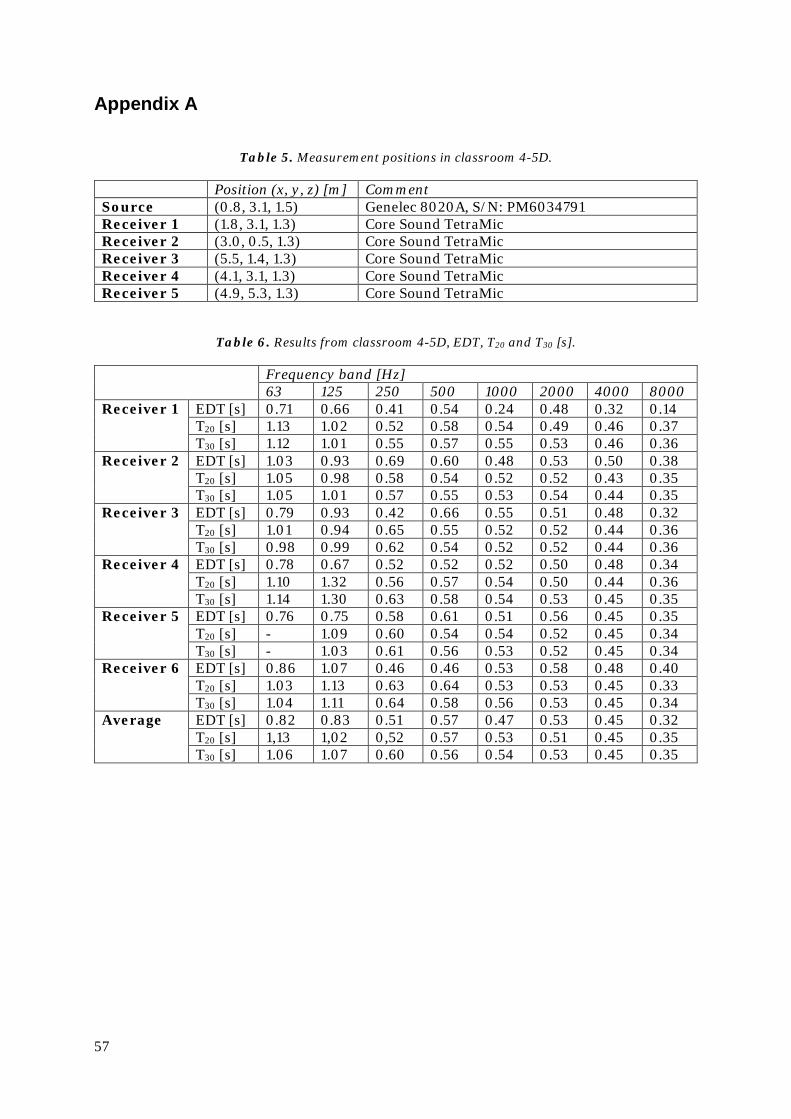
57

Appendix A

Table 5. Measurement positions in classroom 4-5D.

Position (x, y, z) [m] Comment Source (0.8, 3.1, 1.5) Genelec 8020A, S/N: PM6034791 Receiver 1 (1.8, 3.1, 1.3) Core Sound TetraMic Receiver 2 (3.0, 0.5, 1.3) Core Sound TetraMic Receiver 3 (5.5, 1.4, 1.3) Core Sound TetraMic Receiver 4 (4.1, 3.1, 1.3) Core Sound TetraMic Receiver 5 (4.9, 5.3, 1.3) Core Sound TetraMic

Table 6. Results from classroom 4-5D, EDT, T20 and T30 [s].

Frequency band [Hz] 63 125 250 500 1000 2000 4000 8000

Receiver 1 EDT [s] 0.71 0.66 0.41 0.54 0.24 0.48 0.32 0.14 T20 [s] 1.13 1.02 0.52 0.58 0.54 0.49 0.46 0.37 T30 [s] 1.12 1.01 0.55 0.57 0.55 0.53 0.46 0.36




Receiver 5 EDT [s] 0.76 0.75 0.58 0.61 0.51 0.56 0.45 0.35 T20 [s] - 1.09 0.60 0.54 0.54 0.52 0.45 0.34 T30 [s] - 1.03 0.61 0.56 0.53 0.52 0.45 0.34


Average EDT [s] 0.82 0.83 0.51 0.57 0.47 0.53 0.45 0.32 T20 [s] 1,13 1,02 0,52 0.57 0.53 0.51 0.45 0.35 T30 [s] 1.06 1.07 0.60 0.56 0.54 0.53 0.45 0.35

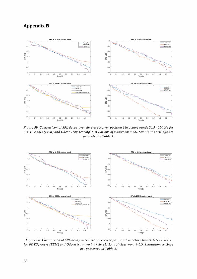
58

Appendix B

Figure 59. Comparison of SPL decay over time at receiver position 1 in octave bands 31.5 - 250 Hz for FDTD, Ansys (FEM) and Odeon (ray-tracing) simulations of classroom 4-5D. Simulation settings are

presented in Table 3.

Figure 60. Comparison of SPL decay over time at receiver position 2 in octave bands 31.5 - 250 Hz for FDTD, Ansys (FEM) and Odeon (ray-tracing) simulations of classroom 4-5D. Simulation settings

are presented in Table 3.

59

Figure 61. Comparison of SPL decay over time at receiver position 3 in octave bands 31.5 - 250 Hz for FDTD, Ansys (FEM) and Odeon (ray-tracing) simulations of classroom 4-5D. Simulation settings are

presented in Table 3.



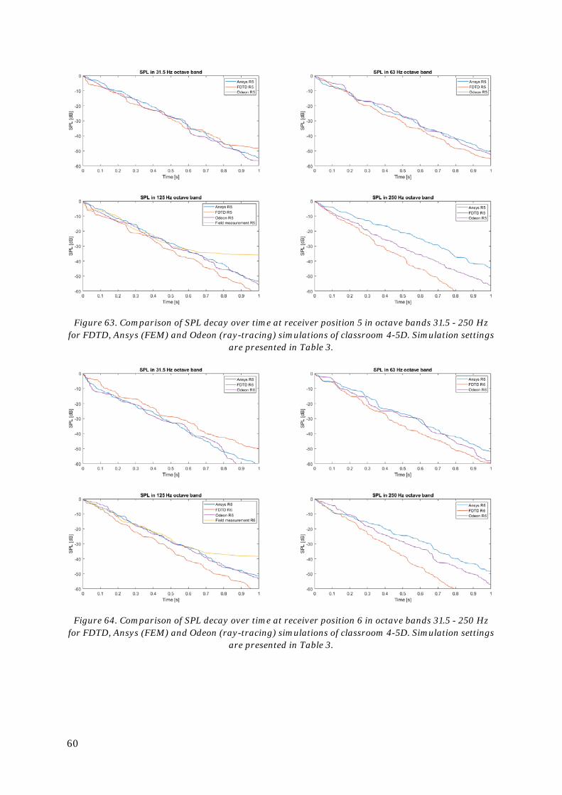
60





www.kth.se

Documents

Simulating Low Frequency Reverberation in Rooms