Embed Size (px)
Citation preview

Journal of Microwaves, Optoelectronics and Electromagnetic Applications, Vol. 15, No. 4, December 2016 DOI: http://dx.doi.org/10.1590/2179-10742016v15i4648
Brazilian Microwave and Optoelectronics Society-SBMO received 11 Apr 2016; for review 13 Apr 2016; accepted 20 Oct 2016
Brazilian Society of Electromagnetism-SBMag © 2016 SBMO/SBMag ISSN 2179-1074
477
Abstract— One of the most recently developed wireless technologies
is Radio Tomographic Imaging (RTI). RTI employs a wireless
sensor network that produces images of the change in the
electromagnetic field of a monitored area using Received Signal
Strength (RSS) measurements. This allows the tracking of device-
free objects such as humans and cars. This paper is the first to
propose and validate a simulation model that simulates RSS
measurements for arbitrary RTI networks, based on the ZigBee
communication protocol. The simulation model allows the
specification of an RTI network from the ground up, including
node positions, network size and geometry and RSS measurement
processing. Furthermore, this paper demonstrates the
implementation of the simulation model to an enhancement of a
recently proposed RTI system, which acts as a roadside
surveillance system. The enhancement includes three newly
proposed techniques, namely a new weight matrix calculation
method, a new node spacing setup and a new vehicle detection
method. The simulation results indicate that it is possible to detect
both one or two family sized cars simultaneously. Using techniques
that reduce RSS variance due to multipath effects and the newly
proposed methods, simulated vehicle detection performance is
demonstrated to be between 95% and 100%.
Index Terms— Radio Tomographic Imaging, Received Signal Strength,
Simulating Wireless Sensor Networks, Vehicle Traffic
I. INTRODUCTION
One of the most recently developed and promising wireless technologies is Radio Tomographic
Imaging (RTI). RTI is a technique that generates an image of the electromagnetic field of a measured
area. Using a mesh network of radios positioned on the borders of the measured area, RTI enables the
localization and tracking of device-free targets. Objects inside the network attenuate the 2.4 GHz ISM
band signals and this attenuation can be measured by obtaining the Received Signal Strength (RSS)
measurements of each link. Retrieved RSS data is used to generate an RTI image, where blobs inside
the image represent the location estimate of a target. Initially developed in 2008 by Patwari et al. [1],
RTI is an emerging and promising technology. Recent relevant RTI research were presented by [2],
[3].
Simulating a Multi-Vehicle Traffic Sensing
System Based on Radio Tomographic Imaging
Jarmo T. Wilkens, Jair A. Silva, Anilton S. Garcia Laboratory of Telecommunications (LabTel), Department of Electrical Engineering, Federal University of
Espírito Santo (UFES), Av. Fernando Ferrari, 514, Campus Goiabeiras, Vitória-ES, Brazil [email protected], [email protected], [email protected]
Journal of Microwaves, Optoelectronics and Electromagnetic Applications, Vol. 15, No. 4, December 2016 DOI: http://dx.doi.org/10.1590/2179-10742016v15i4648
Brazilian Microwave and Optoelectronics Society-SBMO received 11 Apr 2016; for review 13 Apr 2016; accepted 20 Oct 2016
Brazilian Society of Electromagnetism-SBMag © 2016 SBMO/SBMag ISSN 2179-1074
478
Simulating RSS measurements for each link in an RTI system has an important benefit, as it allows
an arbitrary network geometry and size to be evaluated before buying and installing components. This
paper is the first to propose a simulation model that simulates RSS measurements based on a
simulated communication channel in an arbitrary RTI network setup.
Currently, no publications of a proposed simulation model of an RTI system exist. Only two RTI
simulation models exist in literature, which are both proposed in dissertations by Cooke [4] and
Milburn [5]. The simulated RSS data in both cases is reverse engineered using an initial semi-
randomly generated image and mathematical RTI models.
The main limitation of their simulation models is that they lose accuracy of the simulated RSS data
during the process due to their approach of reverse engineering the RSS data. The advantage of the
proposed simulation model over these previous models is that it implements physical layer properties
by simulating a communication channel based on the ZigBee protocol. This makes it possible to
include multipath components and a Rician channel, which both contribute to make the simulated
RSS data more realistic and accurate. Furthermore, it implements the link-channel pair selection
method [3] that reduces multipath effects and RSS behavioral characteristics described in literature to
obtain a more realistic and accurate simulation model. The proposed simulation model allows the
specification of an RTI network from the ground up, including node positions, network size and
geometry, as well as RSS measurement processing using any available or newly developed
techniques. The model is relatively flexible in that it can be used for different types of network
geometries, such as a square geometry as is used in previous works, as well as a front-back geometry
like the one discussed in this paper.
In addition to proposing a new simulation model, this paper presents the implementation of the
simulation model to an enhancement of the recently proposed RTI system by Wilkens et al. [6]. This
RTI system proposes the estimation of the number and velocity of multiple vehicles on a single lane
road segment with radios deployed on the roadside that form an RTI network. The enhancement
includes three newly proposed techniques, namely a new node spacing approach, a new weight matrix
calculation (WMC) method and a new pixel-specific threshold calculation technique for vehicle
detection.
The rest of this paper is organized as follows. Section II discusses the new enhancements
concerning the recently proposed RTI system by Wilkens et al. [6]. Section III describes the proposed
simulation model with validation and implementation of the RTI system. The results after
implementation of the proposed RTI system are presented in section IV and section V concludes this
article.
II. PROPOSED RTI SYSTEM
The proposed RTI system that is simulated is an extension of the RTI system proposed by Wilkens
et al. [6]. Instead of deploying evenly spaced nodes along the roadside, non-linear node spacing was

Journal of Microwaves, Optoelectronics and Electromagnetic Applications, Vol. 15, No. 4, December 2016 DOI: http://dx.doi.org/10.1590/2179-10742016v15i4648
Brazilian Microwave and Optoelectronics Society-SBMO received 11 Apr 2016; for review 13 Apr 2016; accepted 20 Oct 2016
Brazilian Society of Electromagnetism-SBMag © 2016 SBMO/SBMag ISSN 2179-1074
479
chosen to increase link density, and thereby performance, at the sub-network edges. Fig. 1 illustrates
the proposed design as a top view, where the blue circles represent the nodes. Three sub-networks are
displayed, which are justified by Wilkens et al. [6].
Fig. 1. Top view of roadside surveillance proposal
Network scan frequency is dependent on node transmission time and number of channels used. A
trade-off exists between system performance and maximum detectable velocity, where improving
localization accuracy would require using a higher amount of frequency channels due to more reliable
link-channel pairs being selected, which comes at the cost of network scan frequency and thus
maximum detectable velocity. The system proposed by Wilkens et al. [6] has a network scan
frequency of 7 Hz, employs two frequency channels and has a pixel size of 2x2 m2. Fig. 9(a)
visualizes the location of the pixels as blue squares in an arbitrary sub-network.
A. Radio Tomographic Imaging Algorithm
The enhanced algorithm employs the same methods as the recently proposed RTI algorithm [6],
except that it uses a different WMC method, a node-specific path loss model and a new, but similar
pixel-specific threshold technique.
During initialization, the node and pixel locations need to be obtained in order to calculate the
weight matrix W. This weight matrix indicates the extent to which each link represents each pixel.
Node locations are as shown in Fig. 1. The new WMC method is based on placing a circle with radius
0.7 m at the center of each pixel, which is illustrated in Fig. 9(b). All links that pass through the circle
are selected. For the network setup proposed in this paper, this method selects more useful links for
each pixel and thereby leads to improved system performance, as demonstrated in subsection IV.B.1).
Fade level indicates the reliability of a link-channel pair. As demonstrated by Bocca et al. [2], a
higher (lower) fade level generally leads to less (more) RSS link variance. Positive (negative) fade
level links are referred to as anti-fade (deep fade) links, as a result of constructive (destructive)
multipath interference at the receiver. Fade level is calculated using the path loss model and reference
RSS vector. The reference RSS vector is obtained during offline calibration, which is where the
system records RSS data without targets inside the network. To increase accuracy of the fade level,
the path loss model parameters are node specific, as presented by Alippi et al. [3]. In other words,
each node n is modeled to have its own path loss exponent 𝜂𝑛 and transmit reference power 𝑃0𝑛.
Alippi et al. [3] mention that using a node-specific path loss model, the system is more robust against

Journal of Microwaves, Optoelectronics and Electromagnetic Applications, Vol. 15, No. 4, December 2016 DOI: http://dx.doi.org/10.1590/2179-10742016v15i4648
Brazilian Microwave and Optoelectronics Society-SBMO received 11 Apr 2016; for review 13 Apr 2016; accepted 20 Oct 2016
Brazilian Society of Electromagnetism-SBMag © 2016 SBMO/SBMag ISSN 2179-1074
480
hardware variability factors (including relative antenna orientation between communicating radios)
and local environmental differences (like proximity of nodes to dense foliage). The link-channel pair
selection method proposed by Alippi et al. [3] will select the highest quality anti-fade link-channel
pairs that experience least RSS link variance. This filters out unreliable link-channel pairs that
experience deep fading, as well as it filters out the longer distance links that have an average RSS
close to the sensitivity threshold.
The system outputs are the number of detected cars, car location and speed. Every pixel that has an
intensity higher than the pixel-specific threshold is considered to be occupied by a vehicle. This
threshold is new, but similar to the pixel-specific threshold 𝒯𝑣 that was presented by Wilkens et al. [6]
given by:
𝒯v = ρ ( ∑ Fk
k∈𝒜𝑣.
)
1n
(1)
where 𝜌 and n are empirically determined parameters, 𝒜𝑣 is the set of selected link-channel pairs k
covering pixel v and 𝐹𝑘 is the fade level. The basis of this threshold depends on the fact that pixel
intensities in general are lower on network edges than in the network center, due to differences in link
densities respectively, where more (less) RSS information is available in regions with higher (lower)
link densities. Differences in link density along the RTI network can be observed in Fig. 1. Therefore,
the threshold is dependent on amount of selected link-channel pairs given by 𝒜𝑣. A lower threshold is
thus assigned to the border pixels, whereas the center pixels will be given a higher threshold.
Furthermore, the threshold is dependent on fade level, because links with a higher (lower) fade level
lead to a higher (lower) pixel intensity, because they experience more (less) signal attenuation.
Parameters 𝜌 and n shape the threshold curve and are optimized to obtain optimized system
performance. If there are multiple neighboring pixels detected as a car, only the pixel representing the
front part of the car is chosen, so the direction of traffic will need to be known a priori. Vehicle speed
is estimated as the number of pixels displaced per second, multiplied by the pixel width.
The proposed algorithm includes online calibration at the start of each network scan, which helps
reduce RSS time-variance due to random objects being placed inside the network, or weather effects.
III. SIMULATION MODEL
The simulation model is implemented in MATLAB and is based on experimental (raw) data [7] that
Wilson and Patwari published online and which was used in their published article [8]. The
researchers used the Texas Instruments (TI) CC2531 transceiver that communicates through the
ZigBee protocol [9] in the 2.4 GHz ISM band, so the simulation model is based on the ZigBee
protocol (which relies on the IEEE 802.15.4 standard) and the transceiver's properties. The simulation
model is also based on the RSS dynamics outlined by Bocca et al. [2]. Furthermore, this section
Journal of Microwaves, Optoelectronics and Electromagnetic Applications, Vol. 15, No. 4, December 2016 DOI: http://dx.doi.org/10.1590/2179-10742016v15i4648
Brazilian Microwave and Optoelectronics Society-SBMO received 11 Apr 2016; for review 13 Apr 2016; accepted 20 Oct 2016
Brazilian Society of Electromagnetism-SBMag © 2016 SBMO/SBMag ISSN 2179-1074
481
shows how the simulation model can be utilized to implement and evaluate the performance of the
proposed RTI system.
The initialization of the simulation model consists of setting node and pixel locations, calculating
link distances, the weight matrix and regularization matrix. The regularization matrix is further
explained in subsection III.B.5). The simulation model is divided in two sections: subsection III.A
covers the procedure to obtain RSS data, whereas subsection III.B outlines how RSS data is processed
and used to generate new information until a Radio Tomographic Image estimate is obtained. The
procedures detailed in III.A and III.B.1) - III.B.3) only need to be computed once, while III.B.4) -
III.B.6) are repeated for every network scan. The rest of this section demonstrates the model
validation.
A. Obtaining RSS data
The procedure of obtaining RSS data is mainly based on the convolution between a communication
channel, which is modeled as a Rician channel, and a transmitted data signal generated by a simulated
ZigBee protocol for the 2.4 GHz ISM band defined by the IEEE 802.15.4 standard [9]. The output of
the convolution between the transmitted signal (III.A.1) and the Rician channel (III.A.2) with AWGN
is used to obtain the RSS measurements (III.A.3) for each link.
The procedures detailed in this section are repeated for each used frequency channel. In the
simulation model, only the number of frequency channels to be used is specified, rather than the
defining the specific frequency channel.
1) Transmitted signal
Generating a transmitted data signal consists of four stages.
1. The first is to obtain a data frame. The data frame contains the preamble (4 bytes), start frame
delimiter (SFD) (1 byte), frame length field and a reserved bit (total 1 byte) and the data unit. The data
unit contains 2 bytes for the node ID and 1 byte per RSS measured from each node (so 𝑁 − 1 bytes,
where 𝑁 is number of nodes). Therefore, a random (uniformly distributed) binary data sequence of
(7 + 𝑁) × 8 bits is generated.
2. The second stage consists of implementing the Direct Sequence Spread Spectrum (DSSS), by
converting the bits of stage 1 to 4-bit symbols. Afterwards, the symbols are mapped into a 32-chip
pseudorandom (PN) sequence. As the data rate of the original signal is defined to be 250 kb/s [10], the
over-the-air bandwidth after spreading becomes 2 MHz.
3. The third stage modulates the chip sequence with the Offset Quadrature Phase Shift Keying
(OQPSK) modulation scheme.
4. Stage 4 consists of filtering the Q- and I-Phase signals using the Half-Sine pulse shaping filter.
Journal of Microwaves, Optoelectronics and Electromagnetic Applications, Vol. 15, No. 4, December 2016 DOI: http://dx.doi.org/10.1590/2179-10742016v15i4648
Brazilian Microwave and Optoelectronics Society-SBMO received 11 Apr 2016; for review 13 Apr 2016; accepted 20 Oct 2016
Brazilian Society of Electromagnetism-SBMag © 2016 SBMO/SBMag ISSN 2179-1074
482
2) Communication Channel
To model the communication channel, a Rician channel was used, because most of the
communication links are assumed to be Line-of-Sight (LOS), whereas a Rayleigh channel would be
used for non-LOS cases [11].
The number of multipaths is related to the signal bandwidth and coherence bandwidth. Since the
coherence bandwidth is not known a priori, the number of received paths per signal for this simulation
model was chosen to be 3. Therefore, the vectors representing path delays and path gains have three
elements. The first path delay refers to the first arriving path and is set to zero [12]. The subsequent
path delays were set to be random (uniformly distributed) multiples of the sample time of 62.5e-9 s,
where the second path always arrives earlier than the third path.
The path gains are related to the log-distance path loss model parameters found for the "empty area"
data published by Wilson et al. [7]. The parameters found were 𝑃0 = −52.82 dBm at 𝑑0 = 1 m and
𝜂 = 1.57. Around half of all links were simulated to be with positive fade level, which is according to
the data of Wilson et al. [7]. For every link, an initial path gain for the first path was calculated using
the log-distance path-loss model. If that link was detected to be reliable, a gain offset of 5 dB was
added to the initial path gain to give it positive fade level (anti-fade), whereas for unreliable links 5
dB was subtracted from the initial path gain. See section III.C about why a 5 dB gain offset was
chosen. For the subsequent path gains, 2 dB was subtracted from the preceding path gain and a
random (uniformly distributed) decimal value in the interval [-1,1] was added to it. The Rician
channel was then filtered with the transmitted signal. Fig. 5(a) shows the simulated RSS vs. log-
distance and its log-distance path loss model with the same network setup as Wilson et al. [8].
3) Received Signal Strength Measurements
The Received Signal Strength Intensity (RSSI) �̅�𝑙,𝑐 value is obtained by averaging the received
power over the first eight symbols following the SFD directly after the demodulator [9], [10]. Since in
the simulation model the received signal is discrete and shifting from an intermediate frequency to
baseband is not applicable, the RSSI was calculated directly from the received signal without pre-
processing.
B. Processing RSS data
The steps from processing RSS data until a Radio Tomographic Image estimate include computing
fade level, selecting link-channel pairs, calculating thresholds and simulating a vehicle.
1) Fade level
Fade level is dependent on the log-distance path loss model as explained in section II.A. The path
loss parameters 𝜂 and 𝑃0 were calculated by finding the linear model when plotting all simulated RSS
data against the logarithm of corresponding link lengths. Fig. 5(b) shows the fade level of the
simulated RSS with the same network setup as Wilson et al. [7].
Journal of Microwaves, Optoelectronics and Electromagnetic Applications, Vol. 15, No. 4, December 2016 DOI: http://dx.doi.org/10.1590/2179-10742016v15i4648
Brazilian Microwave and Optoelectronics Society-SBMO received 11 Apr 2016; for review 13 Apr 2016; accepted 20 Oct 2016
Brazilian Society of Electromagnetism-SBMag © 2016 SBMO/SBMag ISSN 2179-1074
483
2) Link-channel pair selection
The link-channel pair selection method was first presented by Alippi et al. [3] and contains four
stages.
1. The set of link-channel pairs with positive fade level was obtained.
2. A second set of link-channel pairs was retrieved that contained RSS measurements higher than
the grey region (receiver sensitivity threshold).
3. The intersection between the previously found sets was obtained.
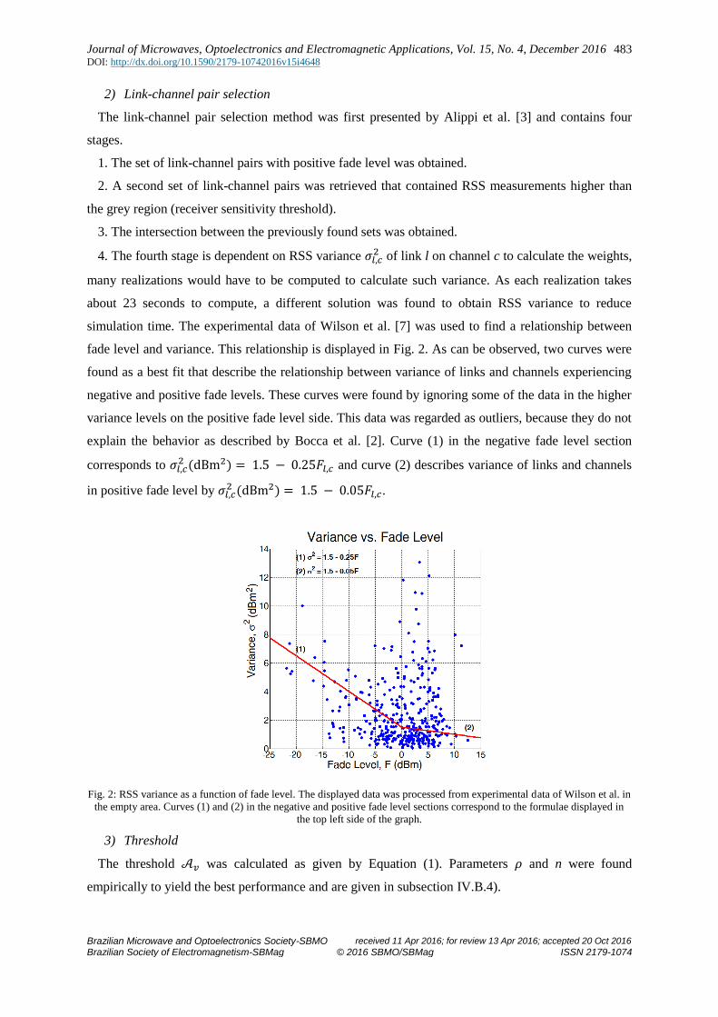
4. The fourth stage is dependent on RSS variance 𝜎𝑙,𝑐2 of link l on channel c to calculate the weights,
many realizations would have to be computed to calculate such variance. As each realization takes
about 23 seconds to compute, a different solution was found to obtain RSS variance to reduce
simulation time. The experimental data of Wilson et al. [7] was used to find a relationship between
fade level and variance. This relationship is displayed in Fig. 2. As can be observed, two curves were
found as a best fit that describe the relationship between variance of links and channels experiencing
negative and positive fade levels. These curves were found by ignoring some of the data in the higher
variance levels on the positive fade level side. This data was regarded as outliers, because they do not
explain the behavior as described by Bocca et al. [2]. Curve (1) in the negative fade level section
corresponds to 𝜎𝑙,𝑐2 (dBm2) = 1.5 − 0.25𝐹𝑙,𝑐 and curve (2) describes variance of links and channels
in positive fade level by 𝜎𝑙,𝑐2 (dBm2) = 1.5 − 0.05𝐹𝑙,𝑐.
Fig. 2: RSS variance as a function of fade level. The displayed data was processed from experimental data of Wilson et al. in
the empty area. Curves (1) and (2) in the negative and positive fade level sections correspond to the formulae displayed in
the top left side of the graph.
3) Threshold
The threshold 𝒜𝑣 was calculated as given by Equation (1). Parameters 𝜌 and n were found
empirically to yield the best performance and are given in subsection IV.B.4).

Journal of Microwaves, Optoelectronics and Electromagnetic Applications, Vol. 15, No. 4, December 2016 DOI: http://dx.doi.org/10.1590/2179-10742016v15i4648
Brazilian Microwave and Optoelectronics Society-SBMO received 11 Apr 2016; for review 13 Apr 2016; accepted 20 Oct 2016
Brazilian Society of Electromagnetism-SBMag © 2016 SBMO/SBMag ISSN 2179-1074
484
4) Vehicle simulation
The procedure described in this subsection contains three stages and was repeated for every network
scan, as it changes the RSS data according to the behavior described by Bocca et al. [2].
1. In the first stage of the simulation model, a vehicle is assumed to be four meters in length, which
corresponds to the length of two neighboring pixels that are a size 2x2 m2 each. All the links chosen
during the weight matrix calculation that represent the pixels occupied by a vehicle are found.
2. All the links in the network are assigned a RSS standard deviation 𝜎𝑙,𝑐 according to the Equations
presented in III.B.2). A new RSS measurement 𝑟𝑙,𝑐 is calculated for each link on each channel by:
rl,c = rl̅,c + σl,c × randn (2)
where �̅�𝑙,𝑐 is the RSS data calculated in III.A.3) and randn is a MATLAB function that generates a
zero mean unit variance random Gaussian variable. This represents the RSS noise, which is assumed
AWGN by Anderson et al. [13].
3. The third stage is where the vehicle is simulated. As shown in an experiment by Bocca et al. [2],
when a target is present on the RSS link in anti-fade, the RSS drops with around 5 dB, while RSS
links in deep fade do not tend to be affected by it due to their high RSS variance. Unfortunately, this
is the only link blocking behavior knowledge available, meaning it was not possible to develop or use
an already existing model to determine the signal attenuation of an arbitrary object size that blocks
links of arbitrary length and fade level. Therefore, a fixed signal attenuation value was used to
subtract from 𝑟𝑙,𝑐 for every anti-fade link-channel pair that is part of the set found in stage 1 of the
described vehicle simulation procedure. The fixed signal attenuation value is set to 8 dB, as it is
assumed that vehicles attenuate signals more than humans do (around 5 dB), but not significantly
more.
5) Obtaining a Radio Tomographic Image estimate
After the RSS vector is updated 𝑟𝑙,𝑐, the change in RSS vector 𝑦𝑙,𝑐 is calculated by 𝑦𝑙,𝑐 = �̅�𝑙,𝑐 − 𝑟𝑙,𝑐.
All the elements in 𝑦𝑙,𝑐 that do not belong to the set of selected link-channel pairs are set to zero.
The radio tomographic image estimate vector �̂� is computed by:
x̂ = Πy (3)
where regularization matrix Π may contain a Tikhonov or covariance matrix [8], [2], where the
former is a more generalized solution and the latter is more specific. For the simulation of the
proposed RTI system, it was chosen to employ general regularization, given by:
Π = (WTW+α(DXTDX+DY
TDY))-1
(4)
where the difference matrices 𝐃X and 𝐃Y are the difference operators for the horizontal and vertical
directions of a 2D image respectively (see [4] for a detailed example). Anderson et al. [13] show that
smoothing parameter 𝛼 can be set to 𝛼 ≈ 0.3 for weak smoothing and 𝛼 ≈ 30 for strong smoothing.

Journal of Microwaves, Optoelectronics and Electromagnetic Applications, Vol. 15, No. 4, December 2016 DOI: http://dx.doi.org/10.1590/2179-10742016v15i4648
Brazilian Microwave and Optoelectronics Society-SBMO received 11 Apr 2016; for review 13 Apr 2016; accepted 20 Oct 2016
Brazilian Society of Electromagnetism-SBMag © 2016 SBMO/SBMag ISSN 2179-1074
485
Removing negative observations in RTI image 𝐱 as proposed by Anderson et al. [13] was
implemented to reduce image noise. This procedure was iterated until the RTI image did not contain
negative pixel intensities anymore, which was never more than one or two iterations.
6) Vehicle detection and speed estimation
The vehicle detection method was implemented exactly as explained in section II.
C. Simulation Validation
To validate the simulation model, all of the data of all 378 links of the experimental RSS data was
combined giving 100,992 measurements. All the RSS data (in voltage) was then shown in one
probability distribution. The application "dfittool" in MATLAB was used to find a distribution that
most closely fits the histogram generated from the RSS data, where the number of bins used was 32.
A distribution was chosen manually and the distribution with highest log likelihood value (calculated
by the application) representing the histogram of the experimental RSS data was selected to represent
the histogram of both experimental and simulated RSS data. It was found that the Burr Type XII
distribution most closely fits the histogram of the experimental RSS data, which are both shown in
Fig. 3.
The next stage in validation was to generate 20 realizations of simulated RSS data, where each
realization contained 100,926 RSS elements. One realization consisted of obtaining one RSS
measurement for each of the 378 links using the method described in section III.A. The rest of the
measurements were simulated by repeating the procedure of the second stage of subsection III.B.4).
All RSS data was converted from dBm to voltage and for each realization, a respective Burr
probability distribution was calculated, which were then averaged to obtain a more generalized result
that is less prone to variations caused by the Rician channel object. The resulting distribution was
validated to the probability distribution of the experimental RSS data according to the Mean Square
Error (MSE) metric of the probability values.
Fig. 3: Histogram of experimental RSS data with its Burr distribution approximation.

Journal of Microwaves, Optoelectronics and Electromagnetic Applications, Vol. 15, No. 4, December 2016 DOI: http://dx.doi.org/10.1590/2179-10742016v15i4648
Brazilian Microwave and Optoelectronics Society-SBMO received 11 Apr 2016; for review 13 Apr 2016; accepted 20 Oct 2016
Brazilian Society of Electromagnetism-SBMag © 2016 SBMO/SBMag ISSN 2179-1074
486
This validation procedure was repeated for four different values of three simulation parameters to
optimize the fit of the simulation distribution to the experimental distribution. The parameters that
were optimized were the path-loss model parameters 𝑃0, 𝜂 and the gain offset, which all affect the
simulated path gains described and hence the shape of the respective RSS probability distribution.
Table 1 presents the MSE values of the three parameters. Fig. 4 presents the optimized simulation
distribution with a MSE of 0.17 × 10⁻⁴ using parameter values 𝑃0 = −50.82 dBm, 𝜂 = 1.37 and
gain offset = 5 dB. Observe that parameter 𝑃0 is the same as obtained from the experimental data, but
parameter 𝜂 was reduced from 1.57 to 1.37. Note that the optimized result presented in this paper is
likely not the best possible result, since only the described parameter values were evaluated. As it
took around 30 minutes to generate one graph, it was left outside the scope of this research to find the
best possible result.
Fig. 4: Burr probability distribution approximation of histogram of experimental RSS data (red line) from Wilson et al. [7]
and simulated data, with path-loss parameters 𝑃0 = −50.82 dBm, 𝜂 = 1.37 and gain offset = 5 dB. MSE = 0.17 × 10⁻⁴
Table 1: Table comparing MSE between Burr probability distribution approximation of histogram of experimental RSS data
and averaged simulated RSS data with different values for 𝑃0, 𝜂 and gain offset
𝜼 MSE (× 𝟏𝟎−𝟒) 𝑷𝟎 (dBm) MSE (× 𝟏𝟎−𝟒) Gain offset (dB) MSE (× 𝟏𝟎−𝟒)
1.17 5.65 -48.82 5.18 1 7.07
1.37 1.85 -49.82 2.46 3 1.82
1.57 4.01 -50.82 1.27 5 0.32
1.77 11.00 -51.82 4.36 7 5.48
Fig. 5(a) and Fig. 5(b) show the simulated RSS vs. log-distance and fade level respectively with the
optimized parameters representing the same network setup as Wilson et al. [8]. As can be observed,
parameters 𝑃0 and 𝜂 are not exactly the same as the optimized parameters, due to the partial
randomness of the Rician channel. Furthermore, the maximum and minimum fade levels
approximately correspond to the experimental fade levels (not presented in this paper).

Journal of Microwaves, Optoelectronics and Electromagnetic Applications, Vol. 15, No. 4, December 2016 DOI: http://dx.doi.org/10.1590/2179-10742016v15i4648
Brazilian Microwave and Optoelectronics Society-SBMO received 11 Apr 2016; for review 13 Apr 2016; accepted 20 Oct 2016
Brazilian Society of Electromagnetism-SBMag © 2016 SBMO/SBMag ISSN 2179-1074
487
(a)
(b)
Fig. 5: Fig. (a) shows simulated RSS (dBm) data versus log-distance (m) and its log-distance path-loss model with
corresponding parameters 𝑃0 and 𝜂 displayed in the graph. Fig. (b) shows the fade level, where the blue and red data points
are the positive and negative fade levels respectively, shown to more easily distinguish between the two levels.

Journal of Microwaves, Optoelectronics and Electromagnetic Applications, Vol. 15, No. 4, December 2016 DOI: http://dx.doi.org/10.1590/2179-10742016v15i4648
Brazilian Microwave and Optoelectronics Society-SBMO received 11 Apr 2016; for review 13 Apr 2016; accepted 20 Oct 2016
Brazilian Society of Electromagnetism-SBMag © 2016 SBMO/SBMag ISSN 2179-1074
488
IV. RESULTS
The results presented in this section demonstrate the implementation of the proposed RTI network
described in section II using the simulation model outlined in section III. In section IV.A, the
optimized result is shown for the implementation of one and two vehicles. How this result was
optimized is covered in section IV.B.
A. Optimized result
This section shows the simulation results of one and two vehicles present inside an arbitrary sub-
network in subsections IV.A.1) and IV.A.2) respectively.
1) Single vehicle
Simulation results of a single family sized car of 4 meters located on each pixel from 1 to 11 in an
arbitrary sub-network is shown in Fig. 6 and Fig. 7, displayed as a line plot and image respectively.
As can be observed in Fig. 6, using the validated simulation model, a car passing through an RTI
network as a roadside surveillance application can clearly be located. A vehicle is detected on any
pixel with pixel intensity higher than the threshold, which, purely by observation, is accurate in each
of 11 cases. The pixel intensities of the car located on the edge of the network is roughly speaking
lower than when it is located in the network's center. This is due to link density, which is lower on the
edge than in the center and the threshold value is adjusted to this characteristic accordingly, showing a
higher value in the middle than on the sides.
Another observation is that the image is still minimally affected by noise, due to RSS link variance
and multipath effects, as seen on the pixels further away from the current vehicle location. Most of the
noise has been filtered out by using the link-channel pair selection method, which is demonstrated in
subsection IV.B.3). The simulation model therefore does not show an ideal case with zero noise, but
rather a more realistic representation of a practical implementation where noise is minimized.
Fig. 7 shows the RTI image version of Fig. 6, where the two brightest neighboring pixels in each
image (a) to (k) represent the location of a vehicle. The pixel intensities are a result of a reconstruction
algorithm given by Equation (3) that uses noisy RSS measurements of selected link-channel pairs.
This is the final output of the RTI technology.

Journal of Microwaves, Optoelectronics and Electromagnetic Applications, Vol. 15, No. 4, December 2016 DOI: http://dx.doi.org/10.1590/2179-10742016v15i4648
Brazilian Microwave and Optoelectronics Society-SBMO received 11 Apr 2016; for review 13 Apr 2016; accepted 20 Oct 2016
Brazilian Society of Electromagnetism-SBMag © 2016 SBMO/SBMag ISSN 2179-1074
489
Fig. 6: Simulated car (black curve) on pixels 1 to 11 (x-axis) shown in Figs. (a) to (k) respectively, where the y-axis
represents pixel intensity. The red dashed curve is the pixel-specific threshold and the arrow indicates the two respective
pixels occupied by the car and the flow direction.
Fig. 7: Simulated car shown as the two brightest neighboring pixels in each image on pixels 1 to 11 shown in Figs. (a) to (k)
respectively. This is the RTI image representation of Fig. 6
2) Two vehicles
This paper proposes the detection and localization of multiple vehicles using the RTI network setup
described in section II. The implementation of this proposal with two vehicles is simulated and
presented in Fig. 8.
The RTI image with two vehicles clearly shows two vehicles located on pixels 2 and 3, and 7 and 8
respectively. The line plot also indicates that the highest intensities are measured on the mentioned
pixels and are all higher than the threshold. This means that in theory, according to the simulation
model and the assumptions made in it, the system would successfully detect the location of both
vehicles in the given scenario. However, system performance is expected to be lower compared to one
vehicle, because some links are blocked by two vehicles at the same time, thereby reducing the
reliability of the respective links.
Journal of Microwaves, Optoelectronics and Electromagnetic Applications, Vol. 15, No. 4, December 2016 DOI: http://dx.doi.org/10.1590/2179-10742016v15i4648
Brazilian Microwave and Optoelectronics Society-SBMO received 11 Apr 2016; for review 13 Apr 2016; accepted 20 Oct 2016
Brazilian Society of Electromagnetism-SBMag © 2016 SBMO/SBMag ISSN 2179-1074
490
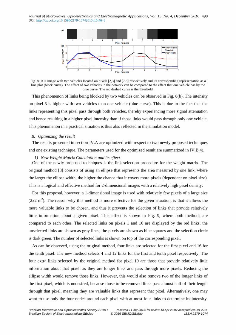
Fig. 8: RTI image with two vehicles located on pixels [2,3] and [7,8] respectively and its corresponding representation as a
line plot (black curve). The effect of two vehicles in the network can be compared to the effect that one vehicle has by the
blue curve. The red dashed curve is the threshold.
This phenomenon of links being blocked by two vehicles can be observed in Fig. 8(b). The intensity
on pixel 5 is higher with two vehicles than one vehicle (blue curve). This is due to the fact that the
links representing this pixel pass through both vehicles, thereby experiencing more signal attenuation
and hence resulting in a higher pixel intensity than if those links would pass through only one vehicle.
This phenomenon in a practical situation is thus also reflected in the simulation model.
B. Optimizing the result
The results presented in section IV.A are optimized with respect to two newly proposed techniques
and one existing technique. The parameters used for the optimized result are summarized in IV.B.4).
1) New Weight Matrix Calculation and its effect
One of the newly proposed techniques is the link selection procedure for the weight matrix. The
original method [8] consists of using an ellipse that represents the area measured by one link, where
the larger the ellipse width, the higher the chance that it covers more pixels (dependent on pixel size).
This is a logical and effective method for 2-dimensional images with a relatively high pixel density.
For this proposal, however, a 1-dimensional image is used with relatively few pixels of a large size
(2x2 m2). The reason why this method is more effective for the given situation, is that it allows the
more valuable links to be chosen, and thus it prevents the selection of links that provide relatively
little information about a given pixel. This effect is shown in Fig. 9, where both methods are
compared to each other. The selected links on pixels 1 and 10 are displayed by the red links, the
unselected links are shown as gray lines, the pixels are shown as blue squares and the selection circle
is dark green. The number of selected links is shown on top of the corresponding pixel.
As can be observed, using the original method, four links are selected for the first pixel and 16 for
the tenth pixel. The new method selects 4 and 12 links for the first and tenth pixel respectively. The
four extra links selected by the original method for pixel 10 are those that provide relatively little
information about that pixel, as they are longer links and pass through more pixels. Reducing the
ellipse width would remove those links. However, this would also remove two of the longer links of
the first pixel, which is undesired, because those to-be-removed links pass almost half of their length
through that pixel, meaning they are valuable links that represent that pixel. Alternatively, one may
want to use only the four nodes around each pixel with at most four links to determine its intensity,

Journal of Microwaves, Optoelectronics and Electromagnetic Applications, Vol. 15, No. 4, December 2016 DOI: http://dx.doi.org/10.1590/2179-10742016v15i4648
Brazilian Microwave and Optoelectronics Society-SBMO received 11 Apr 2016; for review 13 Apr 2016; accepted 20 Oct 2016
Brazilian Society of Electromagnetism-SBMag © 2016 SBMO/SBMag ISSN 2179-1074
491
instead of making use of links that pass through several pixels that just add noise and complexity to
the reconstruction algorithm. In a practical situation, however, it may occur that one or more of these
four links experience deep fade (very unreliable links). Therefore, using only four nodes per pixel,
and filtering out deep fade links, few or maybe no links (in the worst case) may be used to measure
that pixel, thereby making that pixel more inaccurate and vulnerable. See Fig. 5 to notice that short
links are filtered out due to them experiencing deep fade. Hence, as also used in previous RTI works,
it is more desirable to combine information of as much selected link-channel pairs as possible to
measure a pixel. The increased noise and unreliability of links that cover multiple pixels is taken into
account in the more complex weight matrix: shorter links (which cross fewer pixels) are given a larger
weight than longer links.
Vehicle detection performance between the two selection methods is presented in Fig. 10.
Performance was measured by calculating the average detection accuracy (%) of 50 repetitions on
pixels 1 to 11. The output of the performance computation is a 1 or 0 for each repetition, where a 1 is
that the location of the front half of the car is correctly identified and 0 otherwise. In each repetition,
the RSS vector is updated by the procedure described in subsection III.B.4). This process is one
simulation realization, which was repeated 20 times and averaged to obtain a more general result.
Fig. 9: Comparing which links and the amount of links are selected for pixels 1 and 10 using the (a) original and (b) newly
proposed weight matrix calculation (WMC) method. The red and gray lines are the selected and unselected links
respectively, the blue squares are the pixels and the selection circles with radius of 0.7 m are in green.
The performance results indicate that on most pixels, a higher accuracy of between 90% and 100%
is achieved between pixels 1 and 9 using the newly proposed weight matrix calculation (WMC)
method. This already demonstrates that the proposed RTI system will work near perfect according to
the simulation model. Especially a higher accuracy of approximately 100% is yielded on pixels 7 and
8, which are close to the center of the network, due to invaluable links being left out. The edge of the
network shows similar performance between the methods of around 65% to 70%, because in both
cases only 4 links were selected. Pixels 9 and 10 give worst performance, because the pixel intensity
Journal of Microwaves, Optoelectronics and Electromagnetic Applications, Vol. 15, No. 4, December 2016 DOI: http://dx.doi.org/10.1590/2179-10742016v15i4648
Brazilian Microwave and Optoelectronics Society-SBMO received 11 Apr 2016; for review 13 Apr 2016; accepted 20 Oct 2016
Brazilian Society of Electromagnetism-SBMag © 2016 SBMO/SBMag ISSN 2179-1074
492
on pixel 11 is close to the threshold value. When it is higher than the threshold, the system detected
the vehicle location on pixel 11 instead of pixel 10, thereby introducing a False Positive (FP).
Fig. 10: Accuracy (%) of vehicle detection on pixels 1 to 11 with original and new matrix calculation. The data presented are
20 realizations of the original and newly proposed weight matrix calculation (WMC) method and their average.
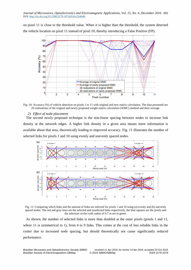
2) Effect of node placement
The second newly proposed technique is the non-linear spacing between nodes to increase link
density at the network edges. A higher link density in a given area means more information is
available about that area, theoretically leading to improved accuracy. Fig. 11 illustrates the number of
selected links for pixels 1 and 10 using evenly and unevenly spaced nodes.
Fig. 11: Comparing which links and the amount of links are selected for pixels 1 and 10 using (a) evenly and (b) unevenly
spaced nodes. The red and gray lines are the selected and unselected links respectively, the blue squares are the pixels and
the selection circles with radius of 0.7 m are in green.
As shown, the number of selected links is more than doubled at the outer pixels (pixels 1 and 11,
where 11 is symmetrical to 1), from 4 to 9 links. This comes at the cost of less reliable links in the
center due to increased node spacing, but should theoretically not cause significantly reduced
performance.

Journal of Microwaves, Optoelectronics and Electromagnetic Applications, Vol. 15, No. 4, December 2016 DOI: http://dx.doi.org/10.1590/2179-10742016v15i4648
Brazilian Microwave and Optoelectronics Society-SBMO received 11 Apr 2016; for review 13 Apr 2016; accepted 20 Oct 2016
Brazilian Society of Electromagnetism-SBMag © 2016 SBMO/SBMag ISSN 2179-1074
493
The effect of node spacing on system performance is illustrated in Fig. 12, which was calculated
using the same performance measuring procedure as in subsection IV.B.1). As can be observed, using
unevenly spaced nodes leads to higher vehicle detection accuracy, especially on the network edges.
This follows exactly the theory of how link density affects performance. System accuracy now is
roughly speaking the same in the edges as in the center of the network, yielding a near perfect
accuracy of between 95 - 100% in the performed experiments.
Fig. 12: Accuracy (%) of vehicle detection on pixels 1 to 11 with evenly and unevenly spaced nodes. The data presented are
20 realizations of the evenly and unevenly spaced nodes (thinner blue and red curves respectively) and their average.
3) Effect of link-channel selection method
According to literature, the more frequency channels that are employed, the higher the quality (with
least RSS variance) of link-channel pairs that are selected.
In the performed simulation experiments shown in Fig. 13, the RTI system demonstrates to be
accurate using only one frequency channel without link-channel pair selection (LCPS), with an
accuracy of between 80% and 90% for all pixels. However, adding a second channel and using the
LCPS method, accuracy for all pixels is significantly improved to between 95% and 100%. A perfect
performance of 100% for all pixels is achieved using four channels and the LCPS method. It is likely
that using three channels would also yield perfect performance, but was not tested for this simulation
comparison. The performance result seen in Fig. 13 can be regarded as another type of simulation
model validation, because the demonstrated performance difference between number of channels used
confirms what is being described in literature.

Journal of Microwaves, Optoelectronics and Electromagnetic Applications, Vol. 15, No. 4, December 2016 DOI: http://dx.doi.org/10.1590/2179-10742016v15i4648
Brazilian Microwave and Optoelectronics Society-SBMO received 11 Apr 2016; for review 13 Apr 2016; accepted 20 Oct 2016
Brazilian Society of Electromagnetism-SBMag © 2016 SBMO/SBMag ISSN 2179-1074
494
Fig. 13: Accuracy (%) of vehicle detection on pixels 1 to 11 without link-channel pair selection (LCPS) and with LCPS (2
and 4 channels). The data presented are 20 realizations of the concerning variables and their average.
The proposed RTI system contains the use of two frequency channels, meaning that in theory, it
performs close to perfect and almost as well as using more than two channels.
Fig. 14 illustrates two RTI images that compare the result of using two and four channels
respectively, with their line plots displayed accordingly. The line plot also shows the result of using
only one channel without LCPS. As expected, the curves with LCPS are very similar to each other
due to their similar system performance, while the curve without LCPS is visibly different. Not only
is the RTI curve different, but also its threshold, which is irregular and seemingly more random as
opposed to the other curved and smooth thresholds. This irregular threshold is likely to have been the
cause of the reduced vehicle detection accuracy. The reason for the irregular threshold is that all fade
levels are included in the calculation, both positive and negative.
Fig. 14: RTI image with vehicle located on pixels 7 and 8 and corresponding line plot without link-channel pair selection
(LCPS) and with LCPS using (a) 2 and (b) 4 channels. The dashed curves in (c) are the thresholds with their color
corresponding to the RTI image they represent.
4) Parameters used for optimized result
The parameters for the threshold 𝜌, 𝑛 and 𝛼 were optimized empirically, by trying out different
values and observing which values yield the best vehicle detection performance. Note that the
optimized values may not be the true best, but merely an approximation, as it is a cumbersome task to
optimize parameters manually. Table 2 summarizes the parameter values used to obtain the optimized
result.

Journal of Microwaves, Optoelectronics and Electromagnetic Applications, Vol. 15, No. 4, December 2016 DOI: http://dx.doi.org/10.1590/2179-10742016v15i4648
Brazilian Microwave and Optoelectronics Society-SBMO received 11 Apr 2016; for review 13 Apr 2016; accepted 20 Oct 2016
Brazilian Society of Electromagnetism-SBMag © 2016 SBMO/SBMag ISSN 2179-1074
495
Table 2: Parameters and their corresponding values and description used for the optimized result.
Parameter Value Description
𝜌 2 Threshold weighting parameter
𝑛 4 Threshold power parameter
𝑟 0.7 Link selection circle radius
𝛼 0.1 Generalized regularization parameter
V. CONCLUSION
This paper proposes a new simulation model that allows the simulation of RSS data in arbitrary RTI
networks. The simulation model was validated by comparing the Burr distribution approximation of
the RSS histograms of the experimental data offered by Wilson et al. [7] and optimized simulated
data. The simulation model was optimized by setting values of three path-loss model parameters that
minimize the MSE between the simulated and reference histograms. An implementation of the
simulation model is presented, which simulates an enhancement of a previously proposed RTI system
by Wilkens et al. [6]. The enhancement includes three newly implemented techniques, namely a new
weight matrix calculation method, a new node spacing setup and a new pixel-specific threshold
calculation approach used for car detection, localization and speed estimation. Simulation results
presented in section IV have demonstrated that the two former newly introduced methods improved
system performance considerably compared to current approaches. The results of the performed
simulated experiments indicate that it is possible to detect both one and two family sized cars
simultaneously in the proposed RTI network setup. Vehicle detection performance is demonstrated to
be between 95% and 100%, which is near perfect, using the new WMC method, new node spacing
setup and using two frequency channels for the link-channel pair selection method. The desired
outcome of this paper is the continuation of the presented research, eventually hoping to deploy the
RTI network as a (complementary) vehicle traffic monitoring structure integrated into an Intelligent
Transport System.
One of the most significant future research is the practical implementation of the proposed RTI
system. To improve simulation model “realisticness”, future research may involve developing a more
sophisticated signal attenuation model. Furthermore, a more advanced technique for vehicle detection
may be implemented using digital image processing techniques. The proposed method of thresholding
is relatively simple and may not perform as well in a practical situation as it did in the simulation
model. Additionally, to minimize RTI system costs, the minimum amount of sensors required to
obtain a given system performance level may be investigated. It would also be interesting to apply
optimization techniques that search for the optimized parameter values automatically.
REFERENCES
[1] N. Patwari and P. Agrawal, "Effects of Correlated Shadowing: Connectivity, Localization, and RF Tomography,"
Information Processing in Sensor Networks, IPSN 2008, pp. 82-93. IEEE, 2008.
[2] M. Bocca, O. Kaltiokallio and N. Patwari, "Radio Tomographic Imaging for Ambient Assisted Living," Evaluating
AAL Systems Through Competitive Benchmarking, pp. 108-130. Springer, 2013.
[3] C. Alippi, M. Bocca, G. Boracchi, N. Patwari and M. Roveri, "RTI Goes Wild: Radio Tomographic Imaging for
Outdoor People Detection and Localization," IEEE, 2014.

Journal of Microwaves, Optoelectronics and Electromagnetic Applications, Vol. 15, No. 4, December 2016 DOI: http://dx.doi.org/10.1590/2179-10742016v15i4648
Brazilian Microwave and Optoelectronics Society-SBMO received 11 Apr 2016; for review 13 Apr 2016; accepted 20 Oct 2016
Brazilian Society of Electromagnetism-SBMag © 2016 SBMO/SBMag ISSN 2179-1074
496
[4] C. Cooke, "Attenuation Field Estimation Using Radio Tomography," Faculty of the Virginia Polytechnic Institute and
State University, Blacksburg, 2011.
[5] A. Milburn, "Algorithms and models for radio tomographic imaging," Leiden University, Leiden, 2014.
[6] J. T. Wilkens and A. S. Garcia, “Design for Multi-Vehicle Roadside Tracking Based on Radio Tomographic
Imaging,” Anais Completo da Programação Técnica. XXXIII Simpósio Brasileiro de Telecomunicações, 2015.
[7] J. Wilson and N. Patwari, "Radio Tomographic Imaging Data Set," Sensing and Processing Across Networks at Utah,
21 Jan 2010. [Online]. Available: http://span.ece.utah.edu/rti-data-set. [Accessed 4 April 2016].
[8] J. Wilson and N. Patwari, "Radio Tomographic Imaging with Wireless Networks," IEEE Transactions on Mobile
Computing, vol. 9, no. 5, pp. 621-632, 2010.
[9] Texas Instruments, "A USB-Enabled System-On-Chip Solution for 2.4-GHz IEEE 802.15.4 and ZigBee
Applications," Texas Instruments, June 2010. [Online]. Available: http://www.ti.com/lit/ds/symlink/cc2531.pdf.
[Accessed 4 April 2016].
[10] IEEE Computer Society, "Part 15.4: Wireless Medium Access Control (MAC) and Physical Layer (PHY)
Specifications for Low-Rate Wireless Personal Area Networks (WPANs)," The Institute of Electrical and Electronics
Engineers, Inc., New York, 2006.
[11] T. S. Rappaport, "Wireless Communications: Principles and Practice. Second Edition," Prentice Hall, 2002, pp. 69-
78, 102-104, 174-176.
[12] MathWorks, "Fading Channels," MathWorks, 2016. [Online]. Available:
http://www.mathworks.com/help/comm/ug/fading-channels.html. [Accessed 4 April 2016].
[13] C. R. Anderson, R. K. Martin, O. T. Walker and R. T. Thomas, "Radio Tomography for Roadside Surveillance,"
IEEE Journal on Selected Topics in Signal Processing, vol. 8, no. 1, pp. 66-79, 2014.
[14] National Instruments, "Pulse-Shape Filtering in Communications Systems," 5 Nov 2014. [Online]. Available:
http://www.ni.com/white-paper/3876/en/. [Accessed 4 April 2016].