Embed Size (px)
Citation preview

1
Simplified Models of the Synchronous Machine
From CC Young’s paper, “Equipment and System Modeling for
Large-Scale Stability Studies,” we read on pg. 1:
and on pg. 2:
And VMAF write (p. 127), that
In a stability study the response of a large number of synchronous machines to a
given disturbance is investigated. The complete mathematical description of the system
would therefore be very complicated unless some simplifications were used. Often only a
few machines are modeled in detail, usually those nearest the disturbance, while others are
described by simpler models. The simplifications adopted depend upon the location of the
machine with respect to the disturbance causing the transient and upon the type of
disturbance being investigated. Some of the more commonly used simplified models are
given in this section. The underlying assumptions as well as the justifications for their use
are briefly outlined. In general, they are presented in the order of their complexity.
Some simplified models have already been presented. In Chapter 2 the classical
representation was introduced. In this chapter, when the saturation is neglected as tacitly
assumed in the current model, the model is also somewhat simplified. An excellent
reference on simplified models is Young [19].
Below is a summary of the different models that we will discuss:

2
Youngs
ID
IEEE ID
(d.q)
Description and relevant
section in the text
G-
cct?
Dmpr
wdgs?
No. of
states
States
Model
III
2.2 Full model with G-cct; see
4.12.
Yes Yes 8 d,F,D,q,
G, Q,,,
2.1 Full model without G-cct. No Yes 7 d,F,D,q,
Q, ,
Model
II
1.1 Machine with solid round
rotor; see 4.15.1.
Yes No 6 d,F,q,G,
,
1.0 E'q model: Same as 1.1 except
for a salient pole machine; see
4.15.1.
No No 5 d,q,E'q,
,
Model
III
2.1 E'' model: for a salient pole
machine & dd/dt= dq/dt=0;
see 4.15.2.
No Yes 5
6 E''d, D,Q,
E'q,,
Model
II
1.1 2-axis model: for a machine
with solid round rotor &
dd/dt= dq/dt=0; see 4.15.3.
Yes No 4 E'd,E'q,,
1.0 One axis model: Same as 2-
axis model (1.1) but without
G-cct; see 4.15.4.
No No 3 E'q,,
Model I 0.0 Classical; see 4.15.5. No No 2 ,
Note that the IEEE ID is useful: d.q, where d indicates how many direct-axis rotor circuits
are modeled (F, D) and q indicates how many quadrature-axis rotor circuits are modeled
(G, Q). Note that these numbers do not include the stator windings (d, q). You can get the
number of electrical states from these numbers according to:
E=d+q+2-N
where “2” is for the d and q winding states and N is the number of states for which the
derivative is assumed zero.
Then, the total number of states is E+M where M=2 is the number of mechanical states.
In the rest of these notes, we summarize the models indicated in
Table 4.6, p. 136, of VMAF (p. 2 of these notes).
Model #
1
2
3
4
5
6
7
8
Observe:
# of states
decrease
from 8
(mod#1) to 2
(mod#8)
First 4 mods
alternate
between rnd-
rot& sal-pole
First 2 mods
have dmprs;
next 2 do not
Mod#5-#8
assume
dd/dt=
dq/dt=0
3
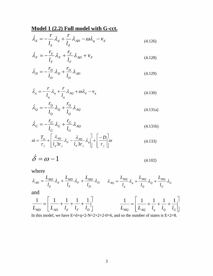
Model 1 (2.2) Full model with G-cct.
(4.126)
(4.128)
(4.129)
(4.130)
(4.131a)
(4.131b)
(4.133)
(4.102)
where
and
In this model, we have E=d+q+2-N=2+2+2-0=6, and so the number of states is E+2=8.
dqAD
d
d
d
d vl
r
l
r
FAD
F
FF
F
FF v
l
r
l
r
AD
D
DD
D
DD
l
r
l
r
qdAQ
q
q
q
q vl
r
l
r
AQ
Q
Q
Q
Q
Q
Ql
r
l
r
AQ
G
GG
G
GG
l
r
l
r
j
q
jd
ADd
jq
AQ
j
m D
ll
T
33
1
D
D
MDF
F
MDd
d
MDAD
l
L
l
L
l
L
G
G
MQ
Q
Q
MQ
q
q
MQ
AQl
L
l
L
l
L
DFdADMD lllLL
11111
GQqAQMQ lllLL
11111

4
Model 2 (2.1): Full model without G-cct.
Same as model 1 except omit the state equation for G (4.131a) &
modify the auxiliary equations, resulting in:
(4.126)
(4.128)
(4.129)
(4.130)
(4.131)
(4.133)
(4.102)
where
and
In this model, we have E=d+q+2-N=2+1+2-0=5, and so the number of states is E+2=7.
dqAD
d
d
d
d vl
r
l
r
FAD
F
FF
F
FF v
l
r
l
r
AD
D
DD
D
DD
l
r
l
r
qdAQ
q
q
q
q vl
r
l
r
AQ
Q
Q
Q
Q
Q
Ql
r
l
r
j
q
jd
ADd
jq
AQ
j
m D
ll
T
33
1
D
D
MDF
F
MDd
d
MDAD
l
L
l
L
l
L Q
Q
MQ
q
q
MQ
AQl
L
l
L
DFdADMD lllLL
11111
QqAQMQ llLL
1111

5
Model 3 (1.1): Machine with solid round rotor. (See page 137)
(No D or Q-axis damper windings).
For this model, VMAF references Kimbark’s Vol. III, saying (p.
137),
“In this model, designated Model 1.1, the G-winding of a solid
round rotor acts as a q axis damper winding, even with the D-
and Q-windings omitted. The mathematical model for this type
of machine will be the same as given in Sections 4.10 and 4.12
with iD or λD omitted and iQ or λQ omitted.”
On checking Kimbark Vol. III, pg. 73, one finds state equations for
both λQ and λD have been dropped, but the G-winding is still there1.
So this model is the same as model 1 except we omit the state
equations for D (4.129) and Q (4.131b), and modify the auxiliary
equations, resulting in:
(4.126)
(4.128)
(4.130)
(4.131a)
(4.133)
(4.102)
1 In the 2nd edition of A&F, the text was assuming no G-winding, whereas Kimbark includes the G-winding.
That is, whereas Kimbark drops both Q and D windings (but retains G), A&F 2nd edition drop only the D
(and retain Q). Thus, A&F 2nd edition implicitly allow the G-winding to substitute for the Q-winding. In both
cases, the model is d.q=1.1, where both have the F-winding which justifies the first “1”; A&F have the Q-
winding (but not G) and Kimbark has the G-winding (but not Q) which justifies (in each case, respectively)
the second “1”. VMAF have reconciled this rather confusing issue by assuming the full model of Sections
4.0 and 4.12 include the G-winding, and the text in VMAF (as quoted above) has been adjusted (relative to
A&F 2nd edition) accordingly.
dqAD
d
d
d
d vl
r
l
r
FAD
F
FF
F
FF v
l
r
l
r
qdAQ
q
q
q
q vl
r
l
r
AQ
G
GG
G
GG
l
r
l
r
j
q
jd
ADd
jq
AQ
j
m D
ll
T
33
1

6
where
and
In this model, we have E=d+q+2-N=1+1+2-0=4, and so the number of states is E+2=6.
Model 4 (1.0): E'q model: Same as #3 except for a salient pole
machine. (See Section 4.15.1, pp. 137-142) (no D- or Q-axis
dampers, and because it is salient pole, omit the G-winding)
One version of this model can be obtained from model 3 (which has
no D- or Q-axis dampers) by omitting the state equation for G
(4.131a) and modifying the Q-axis auxiliary equations
appropriately.
But we may also describe this model in terms of some new “stator-
side” states, E'q, d, and q, which are just scaled versions of three
corresponding rotor quantities. It has been common in the literature
to express machine models in terms of stator-side quantities because
it provides for the ability to efficiently think about (and draw phasor
diagrams for) the magnitudes of the various quantities. VMAF state
(p. 107) “The basis for converting a field quantity to an equivalent
stator EMF is that at open circuit a field current iF A corresponds to
an EMF of iFωReMF V peak” (see p. 17 of perunitization notes).
The three new stator-side quantities are developed below:
E'q is the pu value of the stator equivalent EMF corresponding to
the field flux linkage F, in phase with the q-axis, given by:
(4.203)
This comes about as follows. We call it E’q because it is in phase
with the q-axis. This is the case because it is a voltage due entirely
F
F
MD
d
d
MD
ADl
L
l
L
G
G
MQ
q
q
MQ
AQl
L
l
L
FdADMD llLL
1111
GqAQMQ llLL
1111
F
AD
FqL
LE
3

7
to the field flux, and the field flux is generated along the d-axis.
Because the corresponding induced stator winding voltage is
proportional to dλ/dt, the induced voltage must be 90 degrees out
of phase, meaning it must be along the q-axis.
Its magnitude can be deduced as follows. (This expands on the
discussion in VMAF text, pp. 107-108). Recall that the mutual
inductance between field and a-phase winding (before Park’s
transformation!) is given by tMML FFaF Recoscos (1)
We know that the mutual flux linking the a-phase winding is
FaFaF iL (2)
and that the time derivative of this flux linkage gives the induced
voltage in the a-phase winding, i.e.,
dt
iLd
dt
d FaFaF )(
(3)
Assuming iF is constant, (3) becomes
dt
Ldi
dt
d aFF
aF )(
(4)
Substitution of (1) into (4) yields
tMidt
tMdi
dt
dFF
FF
aFReRe
Re sin)cos(
(5)
and we see that the peak value of the induced a-phase voltage is
ReFFpeak MiE (6)
The RMS value of this voltage would be Vpeak/sqrt(2), i.e.,
Re2
1FFrms MiE (7)
If we multiple both sides by sqrt(3), we get
Re2
33 FFrms MiE (8)
But recall our familiar k=sqrt(3/2), therefore
Re3 FFrms kMiE (9)
To be consistent with the text, we will just use E for Erms, so that
(9) becomes
Re3 FF kMiE (10)
8
Equation (10) is given in your text at the bottom of page 107.
Note that this is the voltage contribution to the a-phase from a
certain value of field current.
VMAF text now considers the case of identifying the a-phase
voltage that results from a certain amount of flux linkage seen by
the field winding λF under steady-state (iQ=iD=0) and open circuit
(id=iq=0) conditions. Under these conditions, the only flux seen
by the field winding is its own flux, and
F
FFFFaF
LiiL
(11)
Substitution of (11) into (10) results in
Re3
F
F
F kML
E (12)
The corresponding voltage is what the book calls E’q, to remind
us that it is a voltage in phase with the q-axis, i.e.,
Re3
F
F
Fq kM
LE (4.59)
We would like to per-unitize the above relation. To do so, recall
the per-unit relations:
FBFBFuFBFuFFBFuFFBFuFBquq ILLLLMkMkMVEE ,,,
Substituting into (4.59), we have that
Re3
FBFu
FBFu
FBFBFuBqu MkM
LL
ILVE
Bring over VB to the right-hand-side & cancel the LFB’s , to obtain
Re3
FBFu
FuB
FBFuqu MkM
LV
IE
Rearranging the right-hand-side
B
FBFBFu
Fu
Fuqu
V
IMkM
LE Re3
Noting that
FBBB
FB
MtV
I 1
we may substitute to obtain

9
Fu
Fu
Fu
FB
FBFu
Fu
Fuqu kM
LMMkM
LE
13
But in pu, kMFu=LAD, and dropping the pu notation results in
AD
F
Fq L
LE
3 (4.203)
We also need to define a “stator-side” quantity corresponding to
the field voltage vF, as vF is our forcing function (and so we need
to obtain the forcing function on the stator-side). This can be
obtained by recognizing that in steady-state, iF=vF/rF. Using (10),
repeated here for convenience,
Re3 FF kMiE
and denoting the stator-side emf as EFD, we have
Re3 F
F
FFD kM
r
vE
Going through a similar process as in previous bullet to convert
to per-unit, we get
(4.209)
Finally, we need to obtain stator-side quantities of
o d, the pu value of the stator equivalent flux linkage
corresponding to the d-winding flux linkage d,
o q, the pu value of the stator equivalent flux linkage
corresponding to the q-winding flux linkage q
o The d- and q- winding voltages vd and vq.
To obtain these, we recall that when we applied Park’s
transformation to a set of balanced a-b-c (stator-side) voltages,
we got:
(4.43)
From (4.203), (4.209), and the (4.43), we conclude that the pu
value of any d or q axis quantity is numerically equal to 3 times
the pu quantity on the stator side. Therefore, the stator-side per-
F
FAD
FDr
vLE
3
cos3
sin3
00
V
V
v
v
v
q
d
10
unit equivalents of rotor side quantities are the rotor side quantity
divided by 3. And so we have:
(4.212)
It is important to realize that E'q (4.203), d, q (4.212), and EFD
(4.209) are given in pu.
With the above relations, we may substitute them into the model 3
state equations and then perform a considerable amount of algebra
to obtain the state equations for the E'q model, given as follows:
In matrix form, equations (4.213-4.215) and (4.219-4.220) become:
We may also generate a block diagram for this model by taking the
LaPlace transform of all equations. The resulting block diagram is
shown in Figures 4.9 and 4.10 of your text, provided below.
3
d
d
3
q
q
3
d
d
vV
3
d
q
vV
1
1
'
1
V
V
01000
00111
000
000
00
0
00
m
j
FD
d
q
d
q
q
d
jdj
q
qd
q
j
dd
d
dd
dd
q
dd
q
q
d
T
EE
D
L
E
LL
L
L
L
LL
L
r
L
r
L
r
E

11
A final comment with respect to this model is that the driving functions
are the inputs EFD (stator-side field voltage which is regulated by the
excitation system), Tm (mechanical power which is regulated by the
turbine-governor system), and the voltages Vd and Vq which are
functions of the external network.
In this model, we have E=d+q+2-N=1+0+2-0=3, and so the number of states is E+2=5.
Comment on dd/dt=dq/dt=0.
Reference to the above table indicates that the E’’ model, the 2-axis
model, the one-axis model, and the classical model all have
dd/dt=dq/dt=0. This issue is addressed in [1, 2], Kundur’s book
Sections 3.7 and 5.1.1 [3], and Krause’s book Chapter 8 [4]. Some
comments about this issue follow:
1. Analysis of a voltage source ( ) sin( )me t E t connected to an
RL circuit will show that the time-domain response of the
current to a short circuit consists of two terms: a transient
unidirectional (DC offset) component and a steady-state
alternating component, i.e., /
1 2( ) sin( )Rt Li t K e K t (*)
2. Each of the three phases of a synchronous machine behave
similarly under the conditions of a bolted three-phase fault

12
applied to the machine terminals at t=0. Kundur [3, p. 107]
illustrates this with the below figure. Here, we observe
a. The DC offset (the dotted line) component decaying
exponentially to zero within about 20 cycles, as represented
in the first term of (*).
b. The fundamental frequency component, as represented in
the second term of (*), except here there is a difference in
that this component has amplitude that also decays with
time to a steady-state value, with
i. the initial rapid decay due to decay of flux linking the
subtransient windings (D and Q) and
ii. the slower decay due to decay of flux linking the
transient windings (F and G).
3. Kundur [3], p. 173, indicates that the effect on power system
stability of the torque corresponding to the DC offset currents
is to produce a DC braking torque which reduces rotor
acceleration following a disturbance. Neglecting it is therefore
conservative; in addition, its effects can be approximated via
another torque term on the right-hand-side of the swing
equation [5], [6, pg. 233-234], [7]. Of most importance,
neglecting it has some major benefits, as follows:
a. There is a similar DC offset effect in the network (it is an
RLC circuit!), but including that effect increases the system
size significantly, contributes high frequency components
(requiring small time steps for numerical integration), and
inhibits use of phasor representation for the network

13
solution part of time-domain simulation. Section 7.3.1 of
VMAF addresses this last point, which is further
characterized by the following statement from [2]: “In stability studies it has been found adequate to represent the network as
a collection of lumped resistances, inductances, and capacitances, and to
neglect the short-lived electrical transients in the transmission
system.[8],[5],[9],[10] As a consequence of this fact, the terminal constraints
imposed by the network appear as a set of algebraic equations which may
be conveniently solved by matrix methods.” b. Neglecting synchronous machine DC offsets and in the
network means that both are being treated consistently.
4. The above figure shows abc (phase) currents. The
corresponding quantities following Park’s transformation are
id and iq, where a. The fundamental frequency components in the phase currents
are reflected as unidirectional components in id and iq. We have
encountered this idea before when we recognized that balanced
steady-state phase (abc) currents transform to DC quantities.
b. The DC offsets in the phase currents are reflected as
fundamental frequency components in id and iq. Neglecting the
DC offset is equivalent to setting did/dt=diq/dt=0, and since our
transformed inductance matrix is constant, setting
did/dt=diq/dt=0 is equivalent to setting dλd/dt=dλq/dt=0.
5. Setting dλd/dt=dλq/dt=0 is referred to in the literature as
“neglecting stator transients” or “neglecting network transients.”
6. Other ways this assumption is expressed include:
a. “transformer voltages are neglected,”
b. “transformer voltages are assumed small compared to
speed voltages” or
c. The stator equations become algebraic.
7. In this case, the state-space equations become, from p. 11 in
“flux linkage equations,” become (changes made to 4.126 and
4.129).
dq
qd

14
0d d AD q d
d d
r rv
l l (4.126)
FAD
F
FF
F
FF v
l
r
l
r (4.128)
0 D D
D D AD
D D
r r
l l (4.129)
qdAQ
q
q
q
q vl
r
l
r (4.130)
AQ
G
GG
G
GG
l
r
l
r
(4.131a)
AQ
Q
Q
Q
Q
Q
Ql
r
l
r
(4.131b)
j
q
jd
ADd
jq
AQ
j
m D
ll
T
33 (4.133)
1 (4.102)

15
Model 5 (2.1): E'' model, for a salient pole machine & dd/dt=
dq/dt=0. See section 4.15.2, p. 142-150.
The intent of this model is to develop a simple model but one that
does account for the effects of both damper windings. So this model
includes both transient and subtransient effects. However, we do not
represent the G-winding, therefore it should only be used for a
salient pole machine.
Recall from our fundamental voltage equations (4.36) that:
(Note the above are in MKS, not per-unit)
An important simplifying assumption for this model is that
(see “Comment on dd/dt=dq/dt=0. on p. 11 of these notes).
We will use E'q as a state, as defined for model 4. But we will also
define one new state:
The d-axis component of the EMF produced by subtransient flux
voltages:
(There is a corresponding q-axis component, defined by e''q=-q,
but it will not be used as a state, since we have E’q.)
There are three basic steps to the development of this model given
in the book. I refer to these steps as Step A, Step B, and Step C. Each
one has several sub-steps, as summarized in what follows:
dqqq
qddd
riv
riv
dq
qd
q d e

16
Step A: Derive the auxiliary equations.
Step A-1: Derive auxiliary equations for e''q and e''d.
1. Substitute expressions for currents id and iq (4.134) into the
equations for ''d and ''q (4.230).
2. Use 3E'q=LADF/LF to write in terms of E'q.
3. Express e''q=q and e''d=-d to get (4.243, 4.245).
Step A-2: Derive the auxiliary equation for E (4.248).
Step A-3: Derive the auxiliary equation for iD.
Step B: Derive the differential equations.
For each of these, we begin from the voltage equation from the
corresponding winding.
Step B-1: D-axis damper: Derive differential equation for D.
Step B-2: Q-axis damper: Derive differential equation for e''d (which
is produced by dq/dt).
Step B-3: Field winding: Derive differential equation for E'q (which
is produced by dF/dt).
State equations are given by (4.263, 4.264, 4.265, 4.267, 4.268).
Step C: Convert to a state-space form:
Step C-1: Convert the state variables to stator-side equivalents by
dividing by 3, and define the constants K1-K4.
Step C-2: Bring in the inertial equations. This results in the
equations of (4.270) in the text, which are written in the LaPlace
domain (with “s” indicating differentiation).
Step C-3: Write equations (4.270) in the time domain and express
them in matrix form to get a state-space model (your book does not
do this part, so you do it).
NOTE: The remainder of these notes are incomplete. Please
read your text p. 142-155.

17
'
''
'
''
q
d
d
q
d
d
E
E
E
E
Note: We have 5 states in this model:
,,E''d,d,E'q
but we are modeling the following windings:
d, q, F, D, Q
With the E'q model (model 4), we only had 3 windings:
d, q, F
but we also had 5 states
,,d,q,E'q
Why is it that we are modeling more windings in the E'' model than
in the E'q model, but we have the same number of states????
Because in the E'' model, we set dd/dt= dq/dt=0, thus eliminating
two stator states.
In this model, we have E=d+q+2-N=2+1+2-2=3, and so the number of states is E+2=5.

18
Model 6 (1.1): “Two-axis model” for a machine with solid round
rotor & dd/dt= dq/dt=0 (pg. 138-140), Section 4.15.3
Overview
This model accounts for the transient effects but not the subtransient
effects. It includes only two rotor circuits, F and G. So we are
neglecting the D- and Q- damper windings. A&F say “The transient
effects are dominated by the rotor circuits which are the field circuit
in the d-axis and an equivalent circuit in the q-axis formed by the
solid rotor.”
The “equivalent circuit in the q-axis formed by the solid rotor” is the
G-circuit (although A&F do not call it that in their second edition).
A&F also write, “An additional assumption made in this model is
that in the stator voltage equations the terms d-dot and q-dot are
negligible compared to the speed voltage terms…” This means that
we let dd/dt= dq/dt=0, as in the E’’ model.
A&F derive two state equations for this model, which are:
0
0
1( ( )
1( )
d d d q q
q
q FD
d
E E x x I
E E E
(4.288), (4.290)
In this model, we have E=d+q+2-N=1+1+2-2=2, and so the number of states is E+2=4.
I will derive the above equations in what follows.
Derivation of (4.288)
From (4.282) we have puG AQ q G GL i L i (4.282)
Differentiating, we obtain: puG AQ q G GL i L i (4.282’)

19
The G-cct voltage equation is 0G G Gr i
Substitute (4.282’) in the G-cct voltage equation to obtain: 0G G AQ q G Gr i L i L i (*)
From (4.286) we have 3 pu
3 (4.286')
3 (4.286'')
d d AQ G
G d
AQ
G d
AQ
E e L i
i EL
i EL
We also have from (4.47) (and see (5.11)) that
3 3q q q qI i I i (4.286’’’)
Substitution of (4.286’), (4.286’’), and (4.286’’’) into (*) results in 3 3
- 3 0G d AQ q G d
AQ AQ
r E L I L EL L
Eliminating the square root of 3, multiplying by -1, and moving
terms to the right-hand-side, results in
G Gd AQ q d
AQ AQ
L rE L I E
L L (#)
Now consider the right-hand equation of (4.287) and its derivative:
( )
( )
d q q d q q
d d q q q
d d q q q
E x I E x I
E E x x I
E E x x I
Substituting into (#) results in
( ) ( )G Gd q q q AQ q d q q q
AQ AQ
L rE x x I L I E x x I
L L
Now expand the terms and then multiply through by LAQ/rG to obtain
2
( ) ( )AQG G
d q q q q d q q q
G G G
LL LE x x I I E x x I
r r r
Now gather terms in qI
21 ( ) ( )G
d G q q AQ q d q q q
G G
LE L x x L I E x x I
r r
and because, in per-unit, xq=Lq and x’q=L’q, we can write the left-
hand-side of the previous expression as

20
21 ( ) ( )G
d G q q AQ q d q q q
G G
LE L L L L I E x x I
r r (*#)
Now we recall from (4.180) that 2
AQ
q q
G
LL L
L (4.180)
Substitution of (4.180) into the left-hand-side of (*#) results in
2
21 ( ) ( )
AQGd G q q AQ q d q q q
G G G
LLE L L L L I E x x I
r r L
which becomes
2 21 ( ) ( )G G
d AQ AQ q d q q q d d q q q
G G G
L LE L L I E x x I E E x x I
r r r
And using 0 /q G GL r from (4.289) we obtain
0q d d q q qE E x x I
which is (4.288) in the A&F text.
QED
Derivation of (4.290)
From (4.280a) puF AD d F FL i L i
Differentiating, we obtain: puF AD d F FL i L i
Substitute the last equation into the voltage equation (4.127)
F F F F F F AD d F F Fr i r i L i L i v (&)
From (4.286) we have 3 3
3 pu
3 pu 3
q AD F F F
AD AD
d d d d
E EE e L i i i
L L
I i I i
(4.286)
And from (4.209),
3 3AD FFD F F FD
F AD
L rE v v E
r L (4.209)
Substitution of these last two relations into (&) results in 3 3
3 3FF AD d F FD
AD AD AD
E E rr L I L E
L L L
Divide through by the square root of 3:
21
FF AD d F FD
AD AD AD
E E rr L I L E
L L L (#0a)
Now recall the left-hand-side of (4.287), and its derivative:
( ) ( )
d d q d d
q d d d q d d d
E x I E x I
E E x x I E E x x I
(#0b)
Substitution of the last two equations in (#0b) into (#0a) results in
( ) ( )F F Fq d d d AD d q d d d FD
AD AD AD
r L rE x x I L I E x x I E
L L L (#0c)
Now, according to the text, just after (4.280), it says: “By
eliminating iF and using (4.174) and (4.203),
3d q d dE L i ” (#1)
Differentiate (#1) to obtain
3d q d dE L i (#2)
But according to the assumptions of this model, 0d , i.e., the left-
hand-side of (#2) is 0, therefore (#2) becomes 3
3q
q d d d
d
EE L i i
L
(#3)
But recall from (4.286) 3 pu 3q q q qI i I i
And so (#3) becomes
q
d
d
EI
L
(#4)
Substitution of (#4) into (#0c) results in
( ) ( )q qF F F
q d d d AD q d d FD
AD d AD d AD
E Er L rE x x I L E x x E
L L L L L
Distributing,
( ) ( )q qF F F F F
q d d d AD q d d FD
AD AD d AD AD d AD
E Er r L L rE x x I L E x x E
L L L L L L L
( ) ( )qF F F F F
q d d d AD d d q FD
AD AD AD d AD AD
Er r L L rE x x I L x x E E
L L L L L L
Bring the first term to the right-hand-side:
FAD d d
AD
TERM A
LL + (x -x ) ( )
L
q F F F Fq FD q d d d
d AD AD AD AD
E L r r rE E E x x I
L L L L L
(#5)

22
Now consider TERM A of (#5), accounting for the fact that in per-
unit, x’d=L’d and xd=Ld, and recalling that L’d=Ld-LAD2/LF:
2 2
F F F FAD d d AD AD AD
AD AD AD AD
L L L LL + (x -x ) L + ( ) L + ( ) L 0
L L L L
AD ADd d d d
F F
L LL L L L
L L
Application of the above TERM A into (#5) results in
( )F F F Fq FD q d d d
AD AD AD AD
L r r rE E E x x I
L L L L (#6)
Multiply through by LAD/LF to obtain
( )F F Fq FD q d d d
F F F
r r rE E E x x I
L L L (#7)
Factor out the rF/LF from the last two terms:
( )F Fq FD q d d d
F F
r rE E E x x I
L L (#8)
Recall from the left-hand-side of (4.287) that ( )q d d dE E x x I
which is recognized in the parentheses of the last term on the right-
hand-side of (#8), so that we have F F
q FD
F F
r rE E E
L L (#9)
Recalling from (4.189) that τ’d0=LF/rF, (#9) becomes
0 0
1 1q FD
d d
E E E
(#10)
which is equation (4.290) in the A&F text.
QED
Model 7 (1.0): One-axis model (4.15.4)
Here, we neglect the dynamics of E’d. In this model, we have E=d+q+2-N=1+0+2-2=1, and so the number of states is E+2=3.
Model 8 (1.0): Classical model.
Here, we assume constant E’q.
In this model, we have E=d+q+2-N=0+0+2-2=0, and so the number of states is E+2=2.

23
[1] Krause, P. C., Nozari, F., Skvarenina, J. L., and Olive, D. W.,
“The Theory of Neglecting Stator Transients,” IEEE Transactions
on PAS, vol. 98, no. 1, pp. 141–148, Jan/Feb 1979.
[2] K. Prabhashankar and W. Janischewsyj, “Digital simulation of
multimachine power systems for stability studies,” IEEE Trans.
Power Apparatus and Systems, Vol. PAS-87, No. 1, January, 1968.
[3] P. Kundur, Power system stability and control, McGraw-Hill,
1994.
[4] P. Krause, O. Wasynczuk, and S. Sudhoff, Analysis of electrical
machinery, IEEE Press, 1994.
[5] R. Harley and B. Adkins, “Calculation of the angular back swing
following a short circuit of a loaded alternator,” Proceedings of the
IEE, Vol. 117, No. 2, pp. 377-386, 1970.
[6] E. Kimbark, Power system stability, Vol. III: Synchronous
Machines, John Wiley, 1956.
[7] D. Mehta and B. Adkins, “Transient torque and load angle of a
synchronous generator following several types of system
disturbance,” Proc. of the IEEE, Vol. 107A, P. 61-74, 1960.