1

Preliminary Fundamentals

1.0 Introduction

In all of our previous work, we assumed a very simple

model of the electromagnetic torque Te (or power) that is

required in the swing equation to obtain the accelerating

torque.

This simple model was based on the assumption that

there are no dynamics associated with the machine

internal voltage. This is not true. We now want to

construct a model that will account for these dynamics.

To do so, we first need to ensure that we have adequate

background regarding preliminary fundamentals, which

include some essential electromagnetic theory, and basics

of synchronous machine construction & operation.

2.0 Some essential electromagnetic theory

2.1 Self inductance

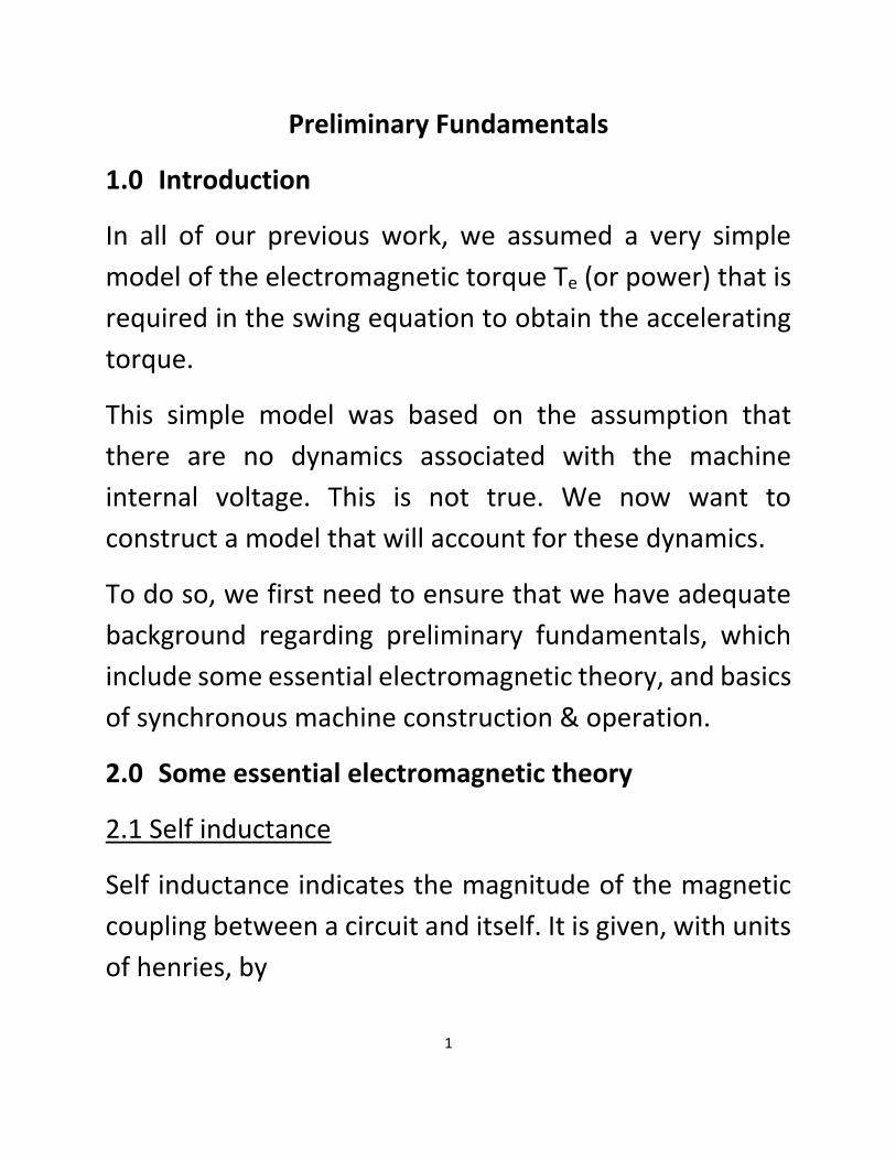
Self inductance indicates the magnitude of the magnetic

coupling between a circuit and itself. It is given, with units

of henries, by

2

1

1111

iL

(1)

We see that the self-inductance L11 is the ratio of

the flux φ11 from coil 1 linking with coil 1, λ11

to the current in coil 1, i1.

Since the flux linkage λ11 is the flux φ11 linking with coil 1,

and since this flux “links” once per turn, and since the

number of turns is N1, then

11111 N (2)

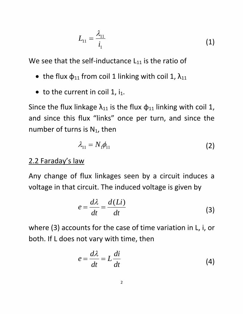
2.2 Faraday’s law

Any change of flux linkages seen by a circuit induces a

voltage in that circuit. The induced voltage is given by

dt

Lid

dt

de

)(

(3)

where (3) accounts for the case of time variation in L, i, or

both. If L does not vary with time, then

dt

diL

dt

de

(4)

3

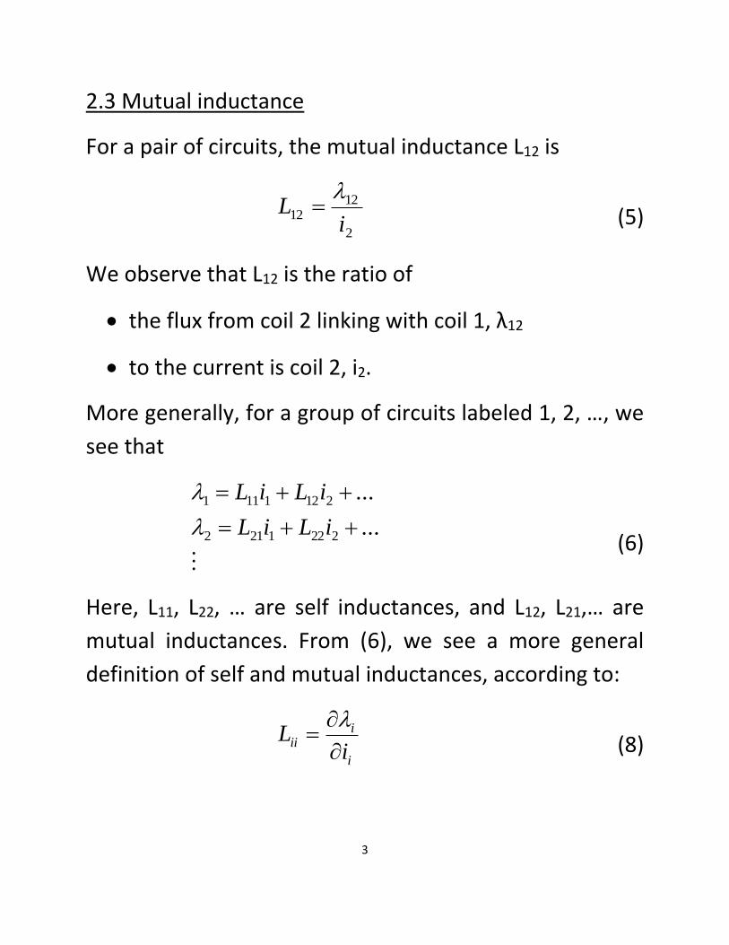
2.3 Mutual inductance

For a pair of circuits, the mutual inductance L12 is

2

1212

iL

(5)

We observe that L12 is the ratio of

the flux from coil 2 linking with coil 1, λ12

to the current is coil 2, i2.

More generally, for a group of circuits labeled 1, 2, …, we

see that

...

...

2221212

2121111

iLiL

iLiL

(6)

Here, L11, L22, … are self inductances, and L12, L21,… are

mutual inductances. From (6), we see a more general

definition of self and mutual inductances, according to:

i

iii

iL

(8)

4

j

iij

iL

(9)

In the case of self inductance, because λi is produced by ii

their directionalities will always be consistent such that

current increases produce flux linkage increases.

Therefore Lii is always positive.

In the case of mutual inductance, whether current

increases in one circuit produce flux linkage increases in

the other circuit depends on the directionality of the

currents and fluxes. The rule we will use is this:

Lij is positive if positive currents in the two circuits produce

self and mutual fluxes in the same direction.

2.4 Inductance and magnetic circuits

We define magnetomotive force (MMF), as the “force”

that results from a current i flowing in N turns of a

conductor. We will denote it with F, expressed by:

NiFMMF (10)

If the conductor is wound around a magnetic circuit

having reluctance R, then the MMF will cause flux to flow

in the magnetic circuit according to

5

RR

NiF (11)

If the cross-sectional area A and permeability μ of the

magnetic circuit is constant throughout, then

A

l

R (12a)

where l is the mean length of the magnetic circuit.

The permeance is given by

RP

1 (12b)

Magnetic circuit relations described above are analogous

to Ohm’s law for standard circuits, in the following way:

FV, φI, RR, PY (13)

So that

R

VI

R

F (14)

We also show in the appendix (see eqs (A8), (A9a)) that

1 2

21 12

N NL L

R 2

111

NL

R (15)

The “F” here should be “F”.

6

2.5 Constant flux linkage theorem

Consider any closed circuit having

finite resistance

flux linkage due to any cause whatsoever

other emf’s e not due to change in λ

no series capacitance

Then

edt

dri

(16)

We know that flux linkages can change, and (16) tells us

how: whenever the balance between the emfs and the

resistance drops become non-zero, i.e.,

riedt

d (17)

But, can they change instantly, i.e., can a certain flux

linkage λ change from 4 to 5 weber-turns in 0 seconds?

To answer this question, consider integrating (16) with

respect to time t from t=0 to t=∆t. We obtain

7

3

0

2

0

1

0

Term

t

Term

t

Term

t

dtedtdt

didtr

(18)

Notice that these terms are, for the interval 0∆t,

Term 1: The area under the curve of i(t) vs. t

Term 2: The area under the curve of dλ/dt vs. t, which is

∆λ(∆t) (read “delta lambda of delta t”).

Term 3: The area under the curve of e(t) vs. t.

Now we know that we can get an instantaneous (step)

change in current

short the circuit or open the circuit,

and we know that we can get an instantaneous (step)

change in voltage

open/close a switch to insert a voltage source into the

circuit.

And so i(t) and/or e(t) may change instantaneously in (18).

But consider applying the limit as Δt0 to (18). In this

case, we have:

8

3

00

2

0

1

00

lim)(limlim

Term

t

t

Term

t

Term

t

tdtetidtr

(19)

Even with a step change in i(t) or e(t), their integrals will

be zero in the limit. Therefore we have:

0)(lim0

2

0

Term

tt

(20)

This implication of (20) is that the flux linkages cannot

change instantaneously. This is the constant-flux-linkage

theorem (CFLT).

CFLT: In any closed electric circuit, the flux linkages will

remain constant immediately after any change in

The current

The voltage

The position of other circuits to which the circuit is

magnetically coupled.

These should be lim as

Δt0 (and not lim as t0).

This should be lim as Δt0

(and not lim as t0).

9

The CFLT is particularly useful when Lii or Lij of a circuit

changes quickly. It allows us to assume λ stays constant so

that we can obtain currents after the change as a function

of currents before the change.

3.0 Basics of synchronous machines

2.1 Basic construction issues

In this section, we present only the very basics of the

physical attributes of a synchronous machine. We will go

into more detail regarding windings and modeling later.

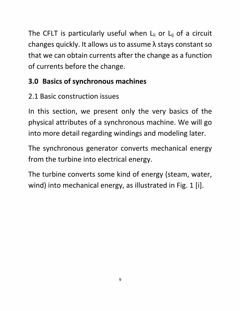
The synchronous generator converts mechanical energy

from the turbine into electrical energy.

The turbine converts some kind of energy (steam, water,

wind) into mechanical energy, as illustrated in Fig. 1 [i].

10

Fig. 1 [i]

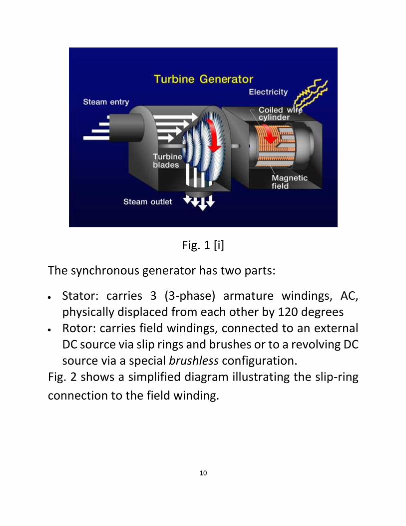
The synchronous generator has two parts:

Stator: carries 3 (3-phase) armature windings, AC, physically displaced from each other by 120 degrees

Rotor: carries field windings, connected to an external DC source via slip rings and brushes or to a revolving DC source via a special brushless configuration.

Fig. 2 shows a simplified diagram illustrating the slip-ring

connection to the field winding.

11

Stator

Stator

winding Slip

rings

Brushes

Rotor

winding

+-

Fig. 2

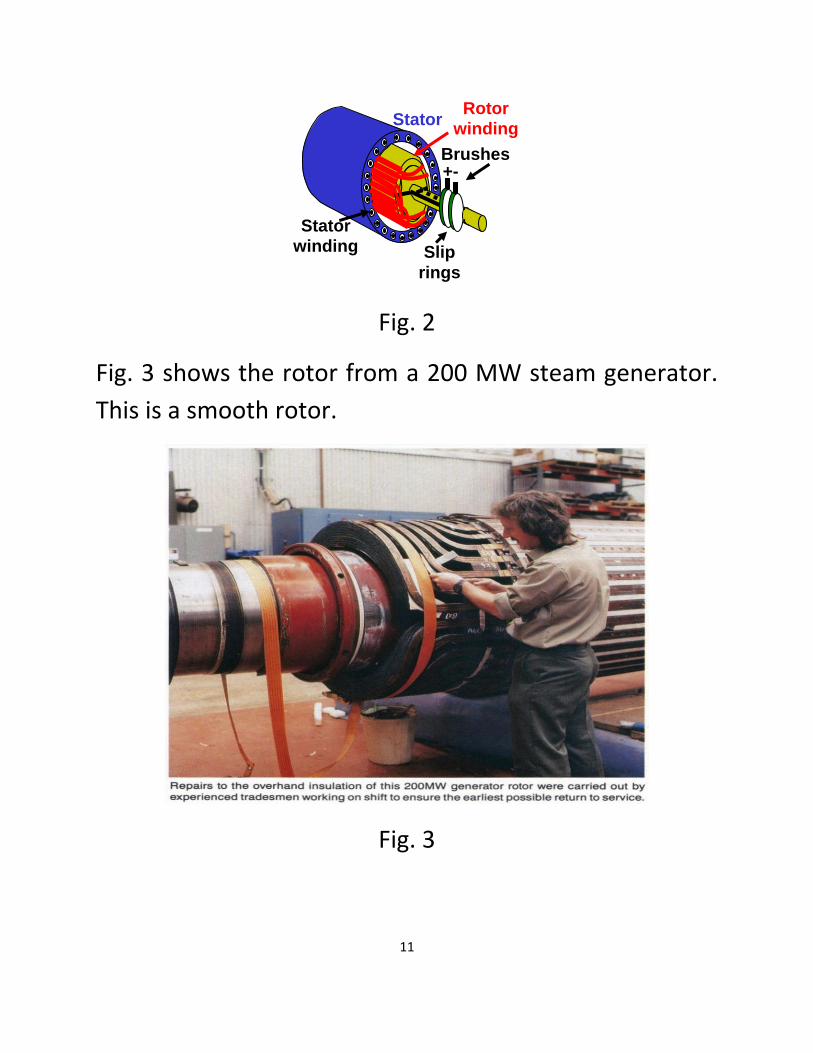
Fig. 3 shows the rotor from a 200 MW steam generator.

This is a smooth rotor.

Fig. 3

12

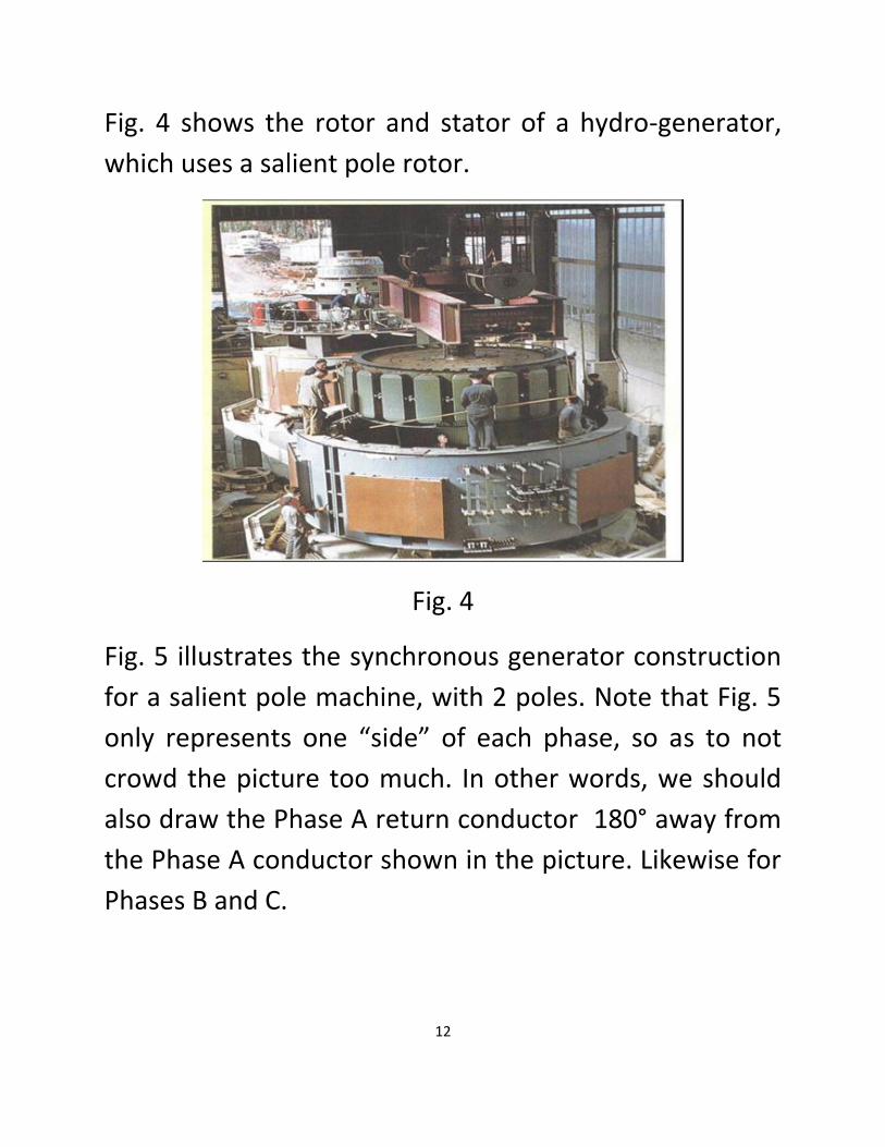
Fig. 4 shows the rotor and stator of a hydro-generator,

which uses a salient pole rotor.

Fig. 4

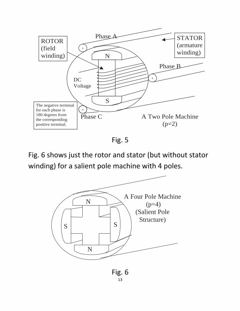
Fig. 5 illustrates the synchronous generator construction

for a salient pole machine, with 2 poles. Note that Fig. 5

only represents one “side” of each phase, so as to not

crowd the picture too much. In other words, we should

also draw the Phase A return conductor 180° away from

the Phase A conductor shown in the picture. Likewise for

Phases B and C.

13

A Two Pole Machine

(p=2)

Salient Pole Structure

N

S

+

+

DC

Voltage

Phase A

Phase B

Phase C

STATOR

(armature

winding)

ROTOR

(field

winding)

The negative terminal

for each phase is

180 degrees from

the corresponding

positive terminal.

+

Fig. 5

Fig. 6 shows just the rotor and stator (but without stator

winding) for a salient pole machine with 4 poles.

A Four Pole Machine

(p=4)

(Salient Pole

Structure)

N

S

N

S

Fig. 6

14

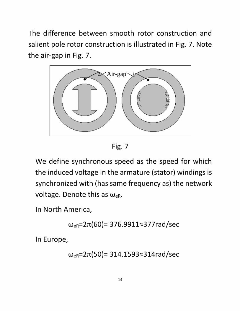
The difference between smooth rotor construction and

salient pole rotor construction is illustrated in Fig. 7. Note

the air-gap in Fig. 7.

Air-gap

Fig. 7

We define synchronous speed as the speed for which

the induced voltage in the armature (stator) windings is

synchronized with (has same frequency as) the network

voltage. Denote this as ωeR.

In North America,

ωeR=2π(60)= 376.9911≈377rad/sec

In Europe,

ωeR=2π(50)= 314.1593≈314rad/sec

15

On an airplane,

ωeR=2π(400)= 2513.3≈2513rad/sec

The mechanical speed of the rotor is related to the

synchronous speed through:

em

p

2

(21)

where both ωm and ωe are given in rad/sec. This may be

easier to think of if we write

me

p

2 (22)

Thus we see that, when p=2, we get one electric cycle

for every one mechanical cycle. When p=4, we get two

electrical cycles for every one mechanical cycle.

If we consider that ωeR must be constant from one

machine to another, then machines with more poles

must rotate more slowly than machines with less.

It is common to express ωmR in RPM, denoted by N; we

may easily derive the conversion from analysis of units:

16

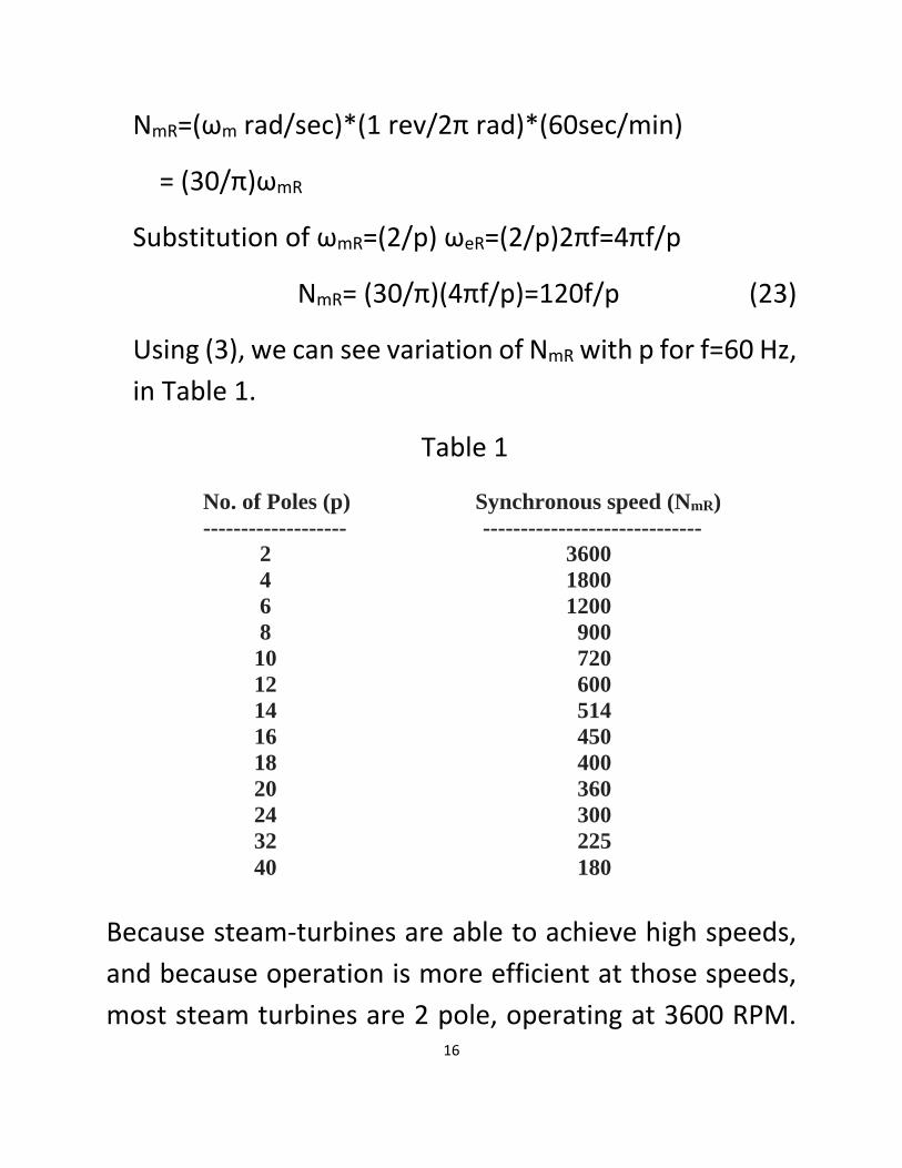
NmR=(ωm rad/sec)*(1 rev/2π rad)*(60sec/min)

= (30/π)ωmR

Substitution of ωmR=(2/p) ωeR=(2/p)2πf=4πf/p

NmR= (30/π)(4πf/p)=120f/p (23)

Using (3), we can see variation of NmR with p for f=60 Hz,

in Table 1.

Table 1

No. of Poles (p) Synchronous speed (NmR)

------------------- -----------------------------

2 3600

4 1800

6 1200

8 900

10 720

12 600

14 514

16 450

18 400

20 360

24 300

32 225

40 180

Because steam-turbines are able to achieve high speeds,

and because operation is more efficient at those speeds,

most steam turbines are 2 pole, operating at 3600 RPM.

17

At this rotational speed, the surface speed of a 3.5 ft

diameter rotor is about 450 mile/hour. Salient poles incur

very high mechanical stress and windage losses at this

speed and therefore cannot be used. All steam-turbines

use smooth rotor construction.

Because hydro-turbines cannot achieve high speeds, they

must use a higher number of poles, e.g., 24 and 32 pole

hydro-machines are common. But because salient pole

construction is less expensive, all hydro-machines use

salient pole construction.

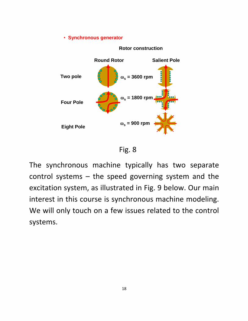
Fig. 8 illustrates several different constructions for smooth

and salient-pole rotors. The red arrows indicate the

direction of the flux produced by the field windings.

18

• Synchronous generator

Rotor construction

Round Rotor Salient Pole

Two pole s = 3600 rpm

Four Poles = 1800 rpm

Eight Poles = 900 rpm

Fig. 8

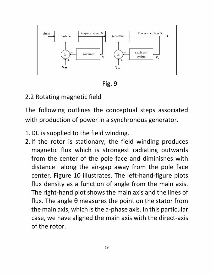
The synchronous machine typically has two separate

control systems – the speed governing system and the

excitation system, as illustrated in Fig. 9 below. Our main

interest in this course is synchronous machine modeling.

We will only touch on a few issues related to the control

systems.

19

Fig. 9

2.2 Rotating magnetic field

The following outlines the conceptual steps associated

with production of power in a synchronous generator.

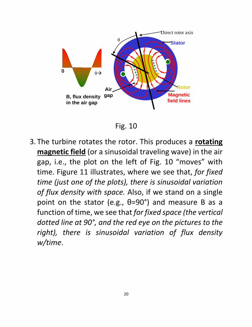
1. DC is supplied to the field winding. 2. If the rotor is stationary, the field winding produces

magnetic flux which is strongest radiating outwards from the center of the pole face and diminishes with distance along the air-gap away from the pole face center. Figure 10 illustrates. The left-hand-figure plots flux density as a function of angle from the main axis. The right-hand plot shows the main axis and the lines of flux. The angle θ measures the point on the stator from the main axis, which is the a-phase axis. In this particular case, we have aligned the main axis with the direct-axis of the rotor.

20

Magnetic

field lines

Stator

RotorAir

gap

0

B, flux density

in the air gap

θ

θ

Direct rotor axis

Fig. 10

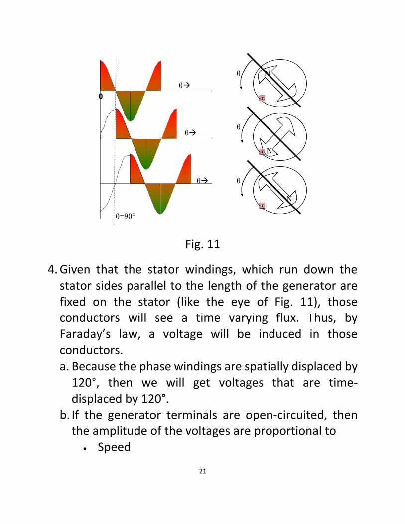
3. The turbine rotates the rotor. This produces a rotating magnetic field (or a sinusoidal traveling wave) in the air gap, i.e., the plot on the left of Fig. 10 “moves” with time. Figure 11 illustrates, where we see that, for fixed time (just one of the plots), there is sinusoidal variation of flux density with space. Also, if we stand on a single point on the stator (e.g., θ=90°) and measure B as a function of time, we see that for fixed space (the vertical dotted line at 90°, and the red eye on the pictures to the right), there is sinusoidal variation of flux density w/time.

21

0

θ

N

N

N

θ

θ

θ

θ

θ

θ=90°

Fig. 11

4. Given that the stator windings, which run down the stator sides parallel to the length of the generator are fixed on the stator (like the eye of Fig. 11), those conductors will see a time varying flux. Thus, by Faraday’s law, a voltage will be induced in those conductors. a. Because the phase windings are spatially displaced by

120°, then we will get voltages that are time-displaced by 120°.

b. If the generator terminals are open-circuited, then the amplitude of the voltages are proportional to

Speed

22

Magnetic field strength And our story ends here if generator terminals are

open-circuited.

5. If, however, the phase (armature) windings are connected across a load, then current will flow in each one of them. Each one of these currents will in turn produce a magnetic field. So there will be 4 magnetic fields in the air gap. One from the rotating DC field winding, and one each from the three stationary AC phase windings.

6. The three magnetic fields from the armature windings will each produce flux densities, and the composition of these three flux densities result in a single rotating magnetic field in the air gap. We develop this here…. Consider the three phase currents:

)240cos(

)120cos(

cos

tIi

tIi

tIi

ec

eb

ea

(24)

Now, whenever you have a current carrying coil, it will

produce a magnetomotive force (MMF) equal to Ni. And

so each of the above three currents produce a time

varying MMF around the stator. Each MMF will have a

23

maximum in space, occurring on the axis of the phase,

of Fam, Fbm, Fcm, expressed as

)240cos()(

)120cos()(

cos)(

tFtF

tFtF

tFtF

emcm

embm

emam

(25)

Recall that the angle θ is measured from the a-phase

axis, and consider points in the airgap. At any time t, the

spatial maximums expressed above occur on the axes of

the corresponding phases and vary sinusoidally with θ

around the air gap. We can combine the time variation

with the spatial variation in the following way:

)240cos()(),(

)120cos()(),(

cos)(),(

tFtF

tFtF

tFtF

cmc

bmb

ama

(26)

Note each individual phase MMF in (26)

varies with θ around the air gap and has an amplitude that varies with time. Substitution of (25) into (26) yields:

24

)240cos()240cos(),(

)120cos()120cos(),(

coscos),(

tFtF

tFtF

tFtF

emc

emb

ema

(27)

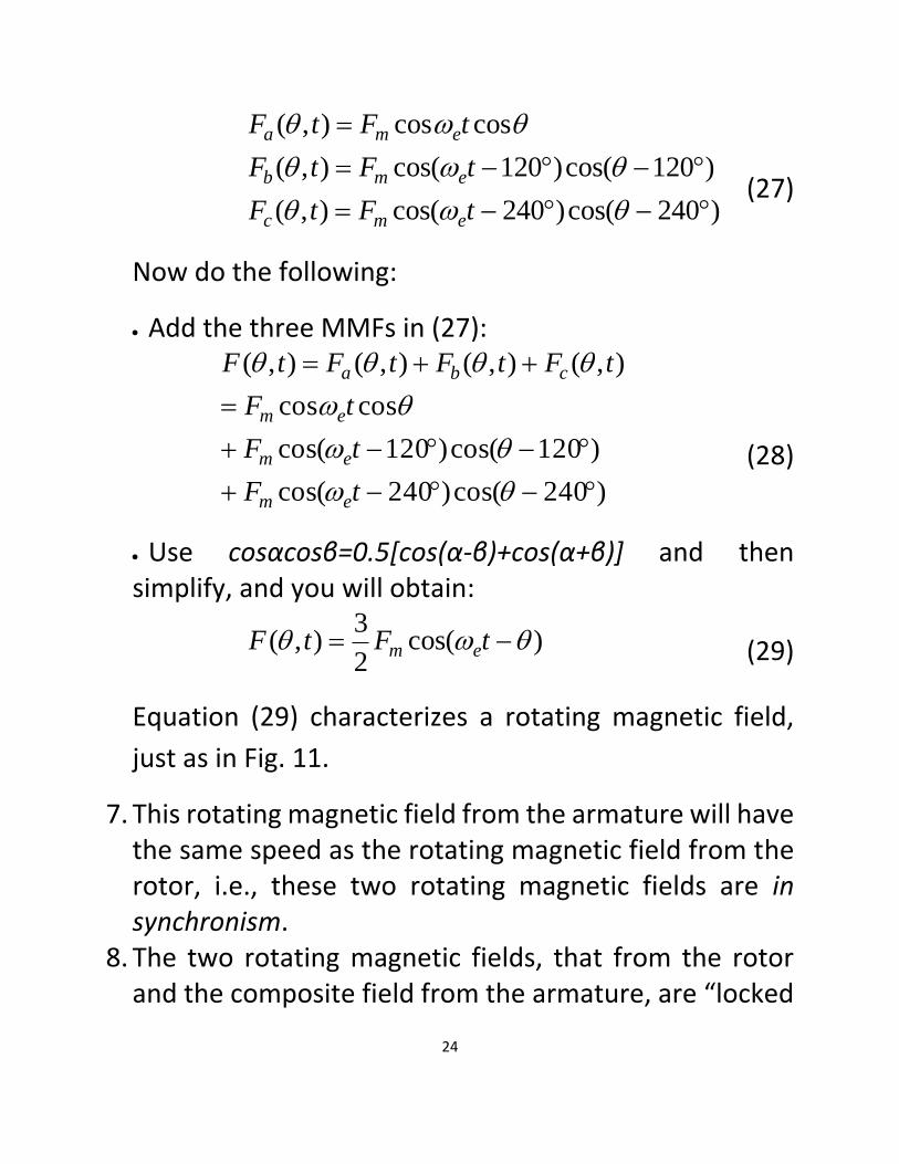
Now do the following:

Add the three MMFs in (27):

)240cos()240cos(

)120cos()120cos(

coscos

),(),(),(),(

tF

tF

tF

tFtFtFtF

em

em

em

cba

(28)

Use cosαcosβ=0.5[cos(α-β)+cos(α+β)] and then simplify, and you will obtain:

)cos(2

3),( tFtF em (29)

Equation (29) characterizes a rotating magnetic field,

just as in Fig. 11.

7. This rotating magnetic field from the armature will have the same speed as the rotating magnetic field from the rotor, i.e., these two rotating magnetic fields are in synchronism.

8. The two rotating magnetic fields, that from the rotor and the composite field from the armature, are “locked

25

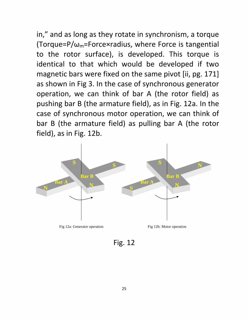
in,” and as long as they rotate in synchronism, a torque (Torque=P/ωm=Force×radius, where Force is tangential to the rotor surface), is developed. This torque is identical to that which would be developed if two magnetic bars were fixed on the same pivot [ii, pg. 171] as shown in Fig 3. In the case of synchronous generator operation, we can think of bar A (the rotor field) as pushing bar B (the armature field), as in Fig. 12a. In the case of synchronous motor operation, we can think of bar B (the armature field) as pulling bar A (the rotor field), as in Fig. 12b.

Fig 12a: Generator operation Fig 12b: Motor operation

N N

S S

Bar A

Bar B

S N

S N

Bar A

Bar B

Fig. 12

26

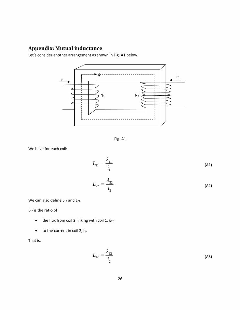
Appendix: Mutual inductance Let’s consider another arrangement as shown in Fig. A1 below.

Fig. A1

We have for each coil:

1

1111

iL

(A1)

2

2222

iL

(A2)

We can also define L12 and L21.

L12 is the ratio of

the flux from coil 2 linking with coil 1, λ12

to the current in coil 2, i2.

That is,

2

1212

iL

(A3)

i1 φ

N1

i2

N2

27

where the first subscript, 1 in this case, indicates “links with coil 1” and the second subscript, 2 in this case,

indicates “flux from coil 2.”

Here, we also have that

2

1211212112

i

NLN

(A4)

Likewise, we have that

1

2121

iL

(A5a)

1

2122121221

i

NLN

(A5b)

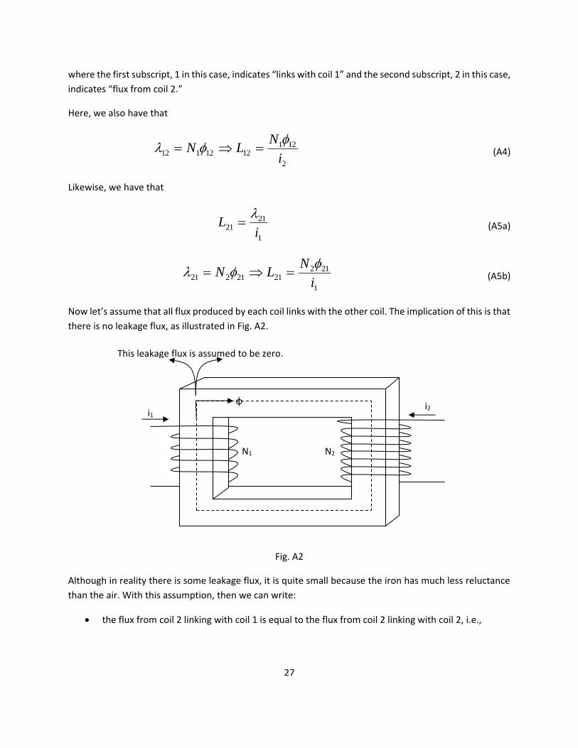
Now let’s assume that all flux produced by each coil links with the other coil. The implication of this is that

there is no leakage flux, as illustrated in Fig. A2.

Fig. A2

Although in reality there is some leakage flux, it is quite small because the iron has much less reluctance

than the air. With this assumption, then we can write:

the flux from coil 2 linking with coil 1 is equal to the flux from coil 2 linking with coil 2, i.e.,

i1 φ

N1

i2

N2

This leakage flux is assumed to be zero.

28

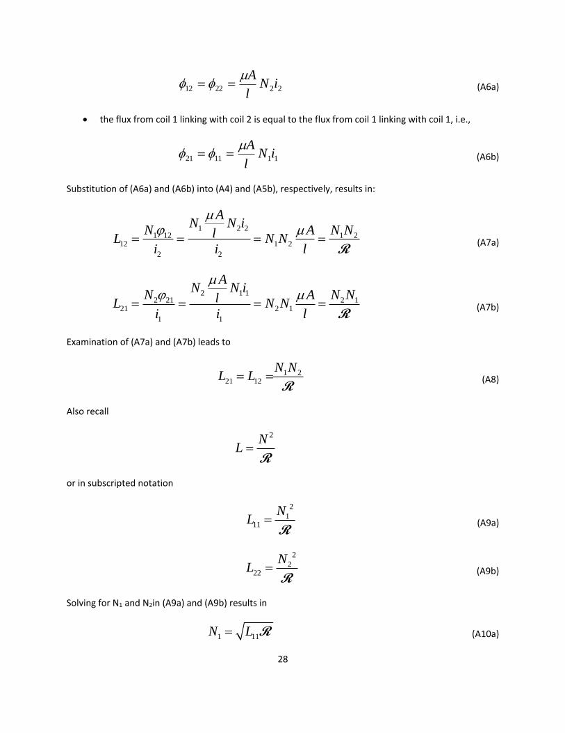
222212 iNl

A (A6a)

the flux from coil 1 linking with coil 2 is equal to the flux from coil 1 linking with coil 1, i.e.,

111121 iNl

A (A6b)

Substitution of (A6a) and (A6b) into (A4) and (A5b), respectively, results in:

1 2 21 12 1 2

12 1 2

2 2

AN N i

N N NAlL N Ni i l

R

(A7a)

2 1 12 21 2 1

21 2 1

1 1

AN N i

N N NAlL N Ni i l

R

(A7b)

Examination of (A7a) and (A7b) leads to

1 221 12

N NL L

R (A8)

Also recall

2NL R

or in subscripted notation

2

111

NL

R (A9a)

2

222

NL

R (A9b)

Solving for N1 and N2in (A9a) and (A9b) results in

1 11N L R (A10a)

29

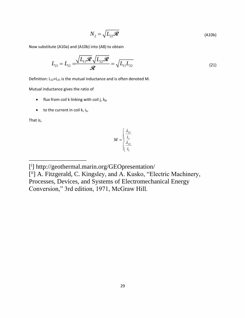
2 22N L R (A10b)

Now substitute (A10a) and (A10b) into (A8) to obtain

11 22

21 12 11 22

L LL L L L

R R

R (21)

Definition: L12=L21 is the mutual inductance and is often denoted M.

Mutual inductance gives the ratio of

flux from coil k linking with coil j, λjk

to the current in coil k, ik,

That is,

1

21

2

12

i

iM

[i] http://geothermal.marin.org/GEOpresentation/

[ii] A. Fitzgerald, C. Kingsley, and A. Kusko, “Electric Machinery,

Processes, Devices, and Systems of Electromechanical Energy

Conversion,” 3rd edition, 1971, McGraw Hill.