Comments Welcome

f thecan beurve

tion isarketsed bye arelar, by

yieldtionsges insimpleshocksodels.micanadian

Bankard of

ish to, Scottf thehuckuciestions.rrors and

Simple Monetary Policy Rules in Canadian Macroeconomic Models:

A Comparison of the Participating Models

by

Denise Côté, John Kuszczak, Jean-Paul Lam, Ying Liu and Pierre St-Amant1

Bank of Canada, Ottawa, Ontario, Canada K1A 0G9

October 2002

Abstract

In this paper, we examine and compare a wide range of private and public sector models oCanadian economy with respect to their paradigm, structure and dynamics properties. The twelve modelsclassified under two economic paradigms. The first one is the “conventional” paradigm (or the Phillips-cparadigm) and the second one is the “money matters” paradigm. Under the conventional paradigm, infladetermined by price adjustments in reaction to inflation expectations and by factor disequilibrium in various m(e.g., the labour market, the goods market). Under the “money matters” paradigm, inflation is mostly determinmovements in monetary aggregates. While most models fall under the “conventional” paradigm, thernevertheless important differences within this paradigm. These differences are represented, in particualternative channels through which monetary policy affects the economy (short-term interest rates or thecurve), by differences in the inflation process (linear/non-linear Phillips curve), by alternative expectaprocesses (backward- or forward-looking expectations), and by the sensitivity of output and inflation to chaninterest rates. We have also examined the dynamic properties of the various models when they use amonetary authority reaction function, such as the one proposed by John Taylor (1993). The eight standardconsidered in our study reveal indeed significant differences in the dynamic properties of the participating mFinally, our comparison of the models’ reaction functions with those of a VAR comprising very little econostructure suggests that some models do a better job than others in reflecting the typical response of the Ceconomy to certain shocks.

1. We would like to thank the following private sector firms and other organizations who have participated in theof Canada project on Taylor Rules including a one-day workshop held on 25 October 2001: Conference BoCanada, DRI-WEFA, IMF, Department of Finance of Canada, OECD and PEAP (University of Toronto). We wthank also Jim day and Samuel Lee for their excellent technical help, Jamie Armour, Ramdane DjoudadHendry, Kevin Moran, Steven Murchison and Bing-Sun Wong for their valuable input and for conducting part osimulations. Finally, we thank Steve Ambler, Don Coletti, Paul Darby, Michael Devereux, Peter Dungan, CFreedman, Alain Guay, Ben Hunt, Douglas Laxton, David Laidler, Andrew Levin, Dale Orr, Benoît Robidoux, LSamson, Jack Selody and all the participants of the “Taylor Rules Workshop” for their comments and suggeThe views expressed in this paper are not those of the Bank of Canada but solely those of the authors. All eomissions are our own.

FR-01-012.

Introduction

hen

y, the

hocks

itted.

one

d of

the

999)

mple

ke it

is to

dian

s in

policy

g key

ty of

nsson

imilar

ntion

tudies

dels fit

of the

simpleof ourCanada

1. Introduction

The monetary authorities must contend with several sources of uncertainty w

conducting monetary policy. The uncertainties they face include the structure of the econom

mechanisms through which monetary policy affects the economy, the nature of the s

affecting that economy and the channels through which these shocks are transm

Consequently, advice regarding monetary policy should be based not solely on

characterization of the economy, but rather on several alternative viewpoints.

When conducting monetary policy, one means of accounting for uncertainty an

mitigating its impact, is to incorporate projections from a variety of different models into

decision-making process. Another approach, proposed by Levin, Wieland and Williams (1

and Taylor (1999) in the context of models of the U.S. economy, consists of using a “si

monetary policy rule”, which yield good results in several models. Such a rule would ma

possible to accommodate uncertainty in economic models. The goal of our research

determine whether we can identify such a rule in the context of models of the Cana

economy.2

Our research is different from the previous literature on simple monetary policy rule

several ways. First, we use a very large number of models to evaluate simple monetary

rules. Second, the models used are very diverse and are all used either for forecastin

variables of the Canadian economy and/or for policy analysis. By considering a large varie

models, we are able to address some of the criticisms, notably by Hetzel (2000) and Sve

(2001), that the models used in the past to evaluate simple monetary policy rules were too s

in structure and did not really constitute a test of robustness of the rules. Third, careful atte

has been paid to how the various models fit the data. Sims (2001) argues that existing s

which use models to evaluate policy rules have not paid enough attention to how these mo

the data. Finally, a robustness check is also performed on the results of our evaluation

monetary policy rules on the basis of a ranking of the participating models.

2. In the fall of 2000, we set out to organize a research framework aim at determining whether we can identify amonetary policy rule in the context of models of the Canadian economy. In the autumn of 2001, the resultsresearch effort were the subject of a Bank of Canada one-day workshop on Taylor Rules (see the Bank ofwebsite at http://www.bankofcanada.ca/workshop2001/).

2 of 41

Introduction

dels

s. This

uent

itled

adian

adian

s, we

in part

cify a

eline

anent)

ted in

modity

k to the

ates.

g and/

rom

re and

ctically

1982,

ructure

ade

s for

ch on

mputer

ations

The goal of this report is to set forth the similarities and differences in the twelve mo

of the Canadian economy with respect to their paradigm, structure and dynamics propertie

will hopefully provide a better understanding of the models in order to facilitate a subseq

evaluation of different simple monetary policy rules, which is subject of another report ent

“The Performance and Robustness of Simple Monetary Policy Rules in Models of the Can

Economy”.

To further understand the structure and properties of the twelve models of the Can

economy, i.e., the way the various models respond to different macroeconomic shock

perform several deterministic simulations. Because output and inflation dynamics depend

on the specification of monetary policy, to compare and evaluate the different models we spe

common policy reaction function. The original Taylor rule is thus imposed as the bas

reaction function in each model. Eight deterministic shocks (seven temporary and one perm

are then simulated in the twelve models. The seven temporary shocks which are simula

these models are as follows: a domestic demand shock, an external shock, a shock to com

prices, a price shock, a wage growth shock, a shock to short-term interest rates, and a shoc

exchange rate. Finally, the deterministic permanent shock is a shock to long-term interest r

The models used in this paper are very diverse and are all used either for forecastin

or for policy analysis. Hence, to find out how and why some or all of the major models differ f

each other is an interesting research avenue in itself. Moreover, recent studies on structu

properties of models of the Canadian economy as well as cross-model comparisons are pra

non-existent. To our knowlegde, the last time that such a study was conducted was in July

when the Bank of Canada and the Department of Finance held a one-day seminar on the st

and properties of nine major Canadian econometric models.3

A number of institutions have since built new models of the Canadian economy or m

major improvements to their models. The passage of time have provided opportunitie

improvements reflecting in part new issues for macroeconomic policy and new resear

economic theory. Also access to new data or more extensive data sets and advances in co

hardware and software and in new algorithms for solving large nonlinear systems of equ

3. See B. O’Reilly, G. Paulin and P. Smith (1983).

3 of 41

Introduction

tunity

ent for

f the

ed on

of a

by the

t and

may

omy.

of

ent

have allowed the creation of more complex models. Our study provides therefore an oppor

to describe the current state of the Canadian macroeconomic models and is a source docum

research studies in macroeconomic modelling in Canada.

The discussion presented in this report, regarding the structure and dynamics o

models of the Canadian economy as well as the analysis of their key properties, is bas

official publications, discussions that we had directly with the participants, the answers

questionnaire on model properties (see Table 1) and on the model responses provided

participants. It is important to keep in mind, however, that the models involved in this projec

described here may still go through ongoing modification. Hence, their current versions

differ from those used in this exercise.

Our study considers twelve private and public sector models of the Canadian econ

Five of them are maintained by private sector organizations. The models are:

i.) CEFM: Canadian Economic and Fiscal Model, Department of Finance Canada;

ii.) DRI: Data Resources of Canada;4

iii.) FOCUS: Policy and Economic Analysis Program (PEAP), Institute for Policy Analysis,University of Toronto;

iv.) FOCUS-CE: the version incorporating forward-looking expectations;

v.) INTERLINK: Organisation for Economic Co-operation and Development;

vi.) MTFM: The Conference Board of Canada’s Medium-Term Forecasting Model;

vii.) WEFA: Wharton Economic Forecasting Associates;

viii.) LPM: Limited Participation Model, Monetary and Financial Analysis Department, BankCanada;

ix.) M1-VECM: Vector-error-correction model, based on the M1 aggregate, Monetary andFinancial Analysis Department, Bank of Canada;

x.) MULTIMOD: International Monetary Fund;

xi.) NAOMI: North American Open-Economy Macroeconometric Integrated Model, Departmof Finance Canada;

xii.) QPM: Quarterly Projection Model, Research Department, Bank of Canada.

4. Data Resources of Canada and Wharton Economic and Forecasting Associates have recently merged.

4 of 41

The Structure and Dynamics of the Models

rtant

he first

While

ences

nnels

rve),

tive

ity of

use a

). The

namic

tions

do a

ertain

more

3, we

inistic

s with

d the

, using

atural

ital, in

Our examination and comparison of the twelve participating models reveal impo

differences among them. The models can be classified under two economic paradigms. T

one is the “conventional” paradigm and the second one is the “money matters” paradigm.

most models fall under the “conventional” paradigm, there are nevertheless important differ

within this paradigm. These differences are represented, in particular, by alternative cha

through which monetary policy affects the economy (short-term interest rates or the yield cu

by differences in the inflation process (linear/non-linear Phillips curve), by alterna

expectations processes (backward- or forward-looking expectations), and by the sensitiv

output and inflation to changes in interest rates.

We have also examined the dynamic properties of the various models when they

simple monetary authority reaction function, such as the one proposed by John Taylor (1993

eight standard shocks considered in our study reveal indeed significant differences in the dy

properties of the participating models. Finally, our comparison of the models’ reaction func

with those of a VAR comprising very little economic structure suggests that some models

better job than others in reflecting the typical response of the Canadian economy to c

shocks.

The remainder of the paper is organized as follows. In Section 2, we examine in

details the twelve models emphasizing the structure and dynamics of each. In Section

discuss the properties of the various models when they are subjected to determ

macroeconomic shocks. In Section 4, we compare some of the models’ response function

those of a vector-autoregressive model. We conclude in Section 5.

2. The Structure and Dynamics of the Models

CEFM

The CEFM5 model incorporates four sectors: firms, households, the government, an

external sector. These sectors are described by a system of 113 estimated equations

61 economic and 52 fiscal variables. Firms maximize profits and use labour, capital, and n

resources to produce goods with a Cobb-Douglas production technology. Demand for cap

5. See Robidoux, B. and B.-S. Wong, 1998. Also see DeSerres, A., B. Robidoux, and B.-S. Wong. 1998.

5 of 41

The Structure and Dynamics of the Models

ction.

dget

r goods

QPM

quidity

hat are

in the

t rate

rated

ict the

illips

vity

turn, is

riable

the

rity’s

nd also

er of

ely the

DRI

nce

upply

rt-term

urve

gap

turn, determines investment in machinery and equipment, and non-residential constru

Consumers maximize utility over an infinite planning horizon subject to an intertemporal bu

constraint. Consequently, consumption, which is disaggregated into purchases of consume

and residential investment, depends on aggregate wealth. As in the MULTIMOD and

models, some consumers are unable to borrow on the basis of future incomes because of li

constraints. The external sector consists of raw materials, finished products, and services t

both exported and imported. The exchange rate is anchored by purchasing-power parity

long run, while deviations from this value are determined by short-term uncovered interes

parity. Compared with the other participating models, the CEFM model has a very elabo

government sector, since one of the principal goals of the Department of Finance is to pred

federal government’s revenue and spending prospects with considerable details.

Inflation, in terms of wage increases, is modelled in CEFM using an augmented Ph

curve with backward-looking inflation expectations. A growth trend in total factor producti

and an unemployment gap are added to these elements. The natural unemployment rate, in

determined by an index of the generosity of the Employment Insurance Program and a va

approximating the level of unionization. The central bank’s instrument for monetary policy is

90-day commercial paper rate. Various reaction functions model the monetary autho

behaviour. Other interest rates are determined through the term structure of interest rates a

exert an influence on the economy’s real variables, such as consumption and investment.

DRI

DRI is a large scale econometric model of about 700 equations with a large numb

variables determined exogenously. The model embodies several sectors which follows clos

National Income and Expenditure Accounts accounting framework. The supply side of the

model is based on an explicit production function yielding potential output. The differe

between actual and potential output is the primary channel through which demand and s

imbalances influences the adjustment of prices. The exchange rate is determined by the sho

uncovered interest rate parity condition and also by movements in real commodity prices.

In DRI, the wage rate is determined in accordance with an extended Phillips c

specification as a function of backward-looking inflation expectations, productivity and the

6 of 41

The Structure and Dynamics of the Models

el, are

ment

ontains

ent of

ations

d by

odel

idered

the IS-

ns.

nt in

ch that

netary

ts of

d as a

urve

lras’s

t rate

age

ation

ation

tations

ns.

between the actual and full-employment unemployment rates. Prices at the producer lev

determined by industrial capacity utilization, the gap between the actual and full-employ

unemployment rates, U.S. wholesale prices and the exchange rate. The financial sector c

several interest rates and the money supply. The 90-day commercial paper rate is the instrum

monetary policy intervention. Longer-term interest rates are determined by the expect

hypothesis and affect real variables such as consumption, housing and investment.

FOCUS

FOCUS6 is a quarterly macroeconomic model of the Canadian economy maintaine

the Policy and Economic Analysis Program (PEAP) of the University of Toronto. The m

consists of a system of some 300 equations and identities. Like most other models cons

here, FOCUS belongs to the neo-classical synthesis. This model’s equations correspond to

LM curve analytical framework and incorporate a Phillips curve with inflation expectatio

Owing to price/wage rigidity, there is a certain trade-off between price and quantity adjustme

the short term. In the long term, however, the model retains a neo-classical character, su

production depends on only real factors and not on variations in aggregate demand. Mo

policy is thus neutral in the long run. Given the large number of equations, the componen

aggregate demand are modelled with considerable detail. Aggregate supply is formulate

Cobb-Douglas production function with decreasing returns to scale. The model’s LM c

defines equilibrium on the money market. Other financial markets are not modelled (Wa

Law). The foreign sector is described with the BP curve, while short-term uncovered interes

parity determines the exchange rate.

In the FOCUS model, the wage adjustment process is similar to that in CEFM. W

changes are modelled using an augmented Phillips curve with backward-looking infl

expectations, to which productivity growth and the unemployment gap are added. Global infl

is thus determined as a markup added to the rate of wage growth. The consistent-expec

version of this model (the “CE” version), incorporates forward-looking inflation expectatio

The instrument of monetary policy intervention is the 90-day commercial paper rate.

6. See Dungan, P. 1997.

7 of 41

The Structure and Dynamics of the Models

short-

ce of

at a

ential

regate

apital

gress.

ent in

s, and

change

rror-

rginal

prices

emand

t from

Wages

epend

edge

te of

GDP

tor and

ward-

paper

affect

as no

INTERLINK

INTERLINK is the OECD’s semi-annual model of the global economy.7 It follows the

tradition of many other macroeconomic models of the neo-classical synthesis, combining

term “keynesian” features with long-term neo-classical properties. In particular, the presen

real and nominal rigidities in the wage and price setting behaviour generally imply th

protracted period of adjustment occurs before output and employment returns to pot

following a shock. The Canadian model, with its 26 equations and 280 identities, has agg

supply determined by a constant-returns-to-scale Cobb-Douglas production function with c

and labour as production factors with the exogenous trend growth rate of technical pro

Aggregate demand is divided into 12 components: private and public consumption, investm

residential and non-residential construction, public sector investment, investment in stock

exports and imports of manufactured and non-manufactured goods and services. The ex

rate is modelled by short-term uncovered interest rate parity.

In INTERLINK, the key price is the business sector GDP deflator, determined in an e

correction framework. In the long-run, prices are determined as a constant mark-up over ma

costs, as calculated from the Cobb-Douglas production function. However, in the short run,

are sensitive to demand pressure and may therefore deviate from trend unit costs. D

pressures also enter through a capacity utilisation term. There is also a short-run effec

import prices of non-manufactures, representing cost pressures from commodity prices.

(including non-wage compensation) come from a reduced-form bargaining model, and so d

on prices, the unemployment rate relative to NAIRU, trend labour productivity, and the w

between consumer and producer prices. Implicitly, the NAIRU is a function of the growth ra

trend labour productivity. Most other prices feed off (are linked to ) the business sector

deflator. For example, the consumption deflator depends on the business sector GDP defla

import prices. Expectations are not specified anywhere in the model except in the back

looking exchange rate equation. Monetary policy operates through the 90-day commercial

rate. Long-term rates have a slightly larger impact than short rates. Long-term interest rates

business investment while short-term interest rates affect consumption. Money growth h

7. See Richardson, P. 1988.

8 of 41

The Structure and Dynamics of the Models

or the

odel

n this

gregate

acity

t-term

-up

output

process

ne: the

shed

to the

mport

nd as

egate

ard-

es in

ent of

ture of

gregate

s of

es. It

ns for

effect in the model and monetary policy does not have a permanent effect on either the level

growth rate of real GDP.

MTFM

The Conference Board of Canada’s MTFM is a large, quarterly, input-output m

comprising about 350 equations. It is estimated on a sample period beginning in 1961. I

model, aggregate demand consists of 70 components. It should be mentioned that ag

supply is not explicitly modelled, although market conditions can be extrapolated from cap

utilization rates by industrial sector. The exchange rate is explained by both uncovered shor

interest rate parity and by commodity price variations.

Global inflation is modelled in the Conference Board’s MTFM using a bottom

approach based on more than 100 different prices whose weights are drawn from input-

tables. Inflationary pressures are established at three main stages of the goods production

(raw materials, intermediate, and finished). Thus, there are three sets of prices to determi

price of raw materials, the price of industrial or transformed products, and the price of fini

products or final demand. At each production stage, price is determined as a markup added

costs of inputs (the marginal cost of labour, the cost of capital, materials, and changes to i

prices). The markup, in turn, is influenced by market conditions, i.e., net aggregate dema

approximated by the utilization rate of production capacity or by the gap between aggr

output and its trend. It should be noted that in MTFM, inflation expectations are backw

looking and, in general, inflation is more sensitive to changes in supply than to chang

aggregate demand. Finally, the central bank uses the treasury bill rate as its instrum

monetary policy. Other rates (e.g., bonds, mortgages) are transmitted over the term struc

interest rates and also play a role, though short-term rates have the greatest impact on ag

demand. Money is neutral in the long term.

WEFA

In many respects, the WEFA model resembles the others. It models four group

economic agents: consumers, firms, budgetary authorities, and monetary authoriti

disaggregates global demand into several components. There are about 10 equatio

9 of 41

The Structure and Dynamics of the Models

lains

t of

s and

y. Note

om

goods-

over

tions

hree-

ructure

of the

onents

three

able),

ough

ney

e the

my’s

ctly

ince

using

consumption and three for investment. A permanent income variable partially exp

consumers’ behaviour. As in the FOCUS, MTFM, and M1-VECM models, the concep

potential output is determined exogenously. As for the financial variables, real interest rate

the exchange rate are linked in the usual manner to short-term uncovered interest rate parit

that this is true of nearly all the models presented in this study.

The WEFA model explains global inflation using a “bottom-up” approach starting fr

several different prices. Inflationary pressures in the economy arise at various stages of the

producing process. Wage increases do not affect prices directly, but rather indirectly

variables for labour income. It should be noted that, in the WEFA model, inflation expecta

are of the backward-looking type. The central bank’s instrument of monetary policy is the t

month treasury bill rate. Other interest rates (e.g., bonds, mortgages) enter over the term st

of interest rates, but do not play a role in the determination of real variables. As in the case

other models, money is neutral in the long term.

LPM

The Limited Participation Model (LPM)8 is a calibrated general-equilibrium model. LPM

decomposes aggregate demand into consumption and investment. Both of these comp

derive from equations of the forward-looking type. In particular, households choose between

classes of consumption goods, two of which are domestic products (tradable and non-trad

while a third is produced abroad. Monetary policy actions affect the real economy thr

frictions generated by agents’ portfolio decisions. More precisely, rigidities in adjusting mo

balances are the main source of the short-run non-neutrality of monetary policy. This is unlik

other participating models, in which the short-term impact of monetary policy on the econo

real variables works over some form of price or wage rigidity. In LPM, prices are perfe

flexible in the short run, implying that the aggregate supply function is vertical. However, s

firms incur debt to finance wages, variations in the interest rate alter supply conditions, ca

the aggregate supply curve to shift.

8. See Hendry, Ho, and Moran, 2001.

10 of 41

The Structure and Dynamics of the Models

is

r key

n the

“money

active

-term

rices

te is

dition

ative

n and

ious

ly. The

and in

is the

ope of

.

el for

odel

hat

term

d-

M1-VECM

The vector-error-correction model (M1-VECM)9 is based on the paradigm that money

at the heart of the monetary policy transmission mechanism. This model comprises fou

equations in which variations in money, production, prices, and interest rates depend o

lagged values of these same variables, on a series of exogenous variables, and on the

gap,” i.e., the difference between money supply and demand. The VECM model assigns an

role to money in the sense that changes in the supply of, relative to the estimated long

demand for, money cause variations in production and in prices in the short term, but only p

in the long term. While the external sector is not explicitly modelled, the exchange ra

determined by uncovered interest rate parity in the short run and anchored in the relative con

of purchasing-power parity in the long run.

M1-VECM assigns an active role to money, in the sense that variations in the rel

supply of, and estimated long-term demand for, money (i.e., the money gap) affect productio

prices jointly. In this model, inflation is measured by core CPI. The money gap in the prev

period and lagged variables for the rate of monetary expansion increase inflation appreciab

lagged output gap, previous variations in the interest rate, in inflation, in the exchange rate,

U.S. interest rates are also accounted for in this model. The monetary policy instrument

overnight fund rate, and the actions of the monetary authorities are transmitted over the sl

the yield curve (overnight rate minus the rate on bonds with maturities exceeding 10 years)

MULTIMOD

MULTIMOD is the IMF’s annual model of the global economy.10 It includes individual

models for each of the seven largest industrialized countries (including Canada), one mod

the remaining 14 industrialized countries, one model for developing countries, and a final m

for countries in transition. Like QPM, MULTIMOD consists of a set of dynamic relationships t

trace the path leading from the starting conditions to the implicit steady-state, or long-

equilibrium, solution. In MULTIMOD,11 consumer behaviour is modelled on the Blanchar

9. See Adam, C. and S. Hendry. 2000.

10. The model is estimated for the 1970–2000 period.

11. See Laxton, D. et al. 1998.

11 of 41

The Structure and Dynamics of the Models

on.

ght of

vary

cycle.

ty to

ed by

sable

l of

uctivity

tively

estic

e

ed by

t rates

te real

sary for

rly

oth

the

the

tions

inear

istent

ed by

ively.

Weil-Buiter paradigm,12 which assumes that economic agents plan within a finite time horiz

Consumers’ lifespans are unknown, and they must plan their consumption and savings in li

this uncertainty. This paradigm is extended with the addition of remuneration profiles that

across age groups and imply different marginal propensities to consume over the life

Moreover, consumers are confronted, in part, with liquidity constraints that restrict their abili

borrow on the basis of future income. Thus, in this model, aggregate consumption is obtain

summing consumption depending on permanent income with that depending on dispo

income.

MULTIMOD models investment with Tobin’s q, which specifies that the desired leve

investment may exceed the steady-state level to the extent that the expected marginal prod

of capital is greater than its replacement cost. The specification of the foreign sector is rela

conventional. Imports are determined by their relative prices and by a measure of dom

activity calibrated on the basis of input-output tables.13 Exports are modelled to be compatibl

with other countries’ imports. In the short term, exchange rates and interest rates are link

uncovered interest rate parity adjusted for risk premiums. As in QPM, real domestic interes

are connected to exogenous foreign values adjusted for risk premiums, while the steady-sta

exchange rate is determined endogenously to generate the trade balance flows neces

overall equilibrium in the economy’s stock of assets.

The MULTIMOD models fundamental inflation (defined as core CPI inflation) simila

to QPM—i.e., using a non-linear Phillips curve with inflation expectations that are b

backward- and forward-looking—except that the disequilibrium factor is approximated by

unemployment gap.14 Global inflation, that is, the overall rise in the CPI, includes changes in

prices of imports of manufactured goods, the rate of growth of the price of oil, previous varia

in global inflation, and the rate of increase in the core CPI. Expected inflation, in turn, is a l

combination of previous values of the growth rate of the CPI, the core CPI, and model-cons

12. Buiter, W.H. 1988.

13. MULTIMOD is a macroeconomic model of the world economy. The share of domestic demand suppliforeign production is established on the basis of input-output tables specific to each country.

14. In MULTIMOD, the backward-looking and forward-looking elements are weighted 0.75 and 0.25, respect

12 of 41

The Structure and Dynamics of the Models

hort-

rget.

1, the

ood

real

model

entire

tion

tput,

real

of the

tor is

ative

nomy

ing

lative

utput

vel of

tary

real

its

values for those two measures. In MULTIMOD, monetary authorities act on the nominal s

term interest rate, i.e., the three-month treasury bill rate, to achieve their inflation-control ta

NAOMI

The North American Open-Economy Macroeconometric Integrated Model15 (NAOMI)

includes six behavioural equations and 18 identities. For the sample period, 1972Q1–2000Q

equation system is estimated simultaneously using the full-information maximum-likelih

(FIML) procedure. The model’s endogenous variables include output growth, inflation, the

exchange rate, the yield curve, and long-term interest rates. Variables exogenous to the

include potential output, U.S. variables, commodity prices, and the budget balance for the

public sector. Like M1-VECM, NAOMI defines aggregate demand in terms of a single equa

(IS curve). In particular, production growth is modelled on increases in potential ou

production growth in the United States, and changes in the yield curve. Variations in the

exchange rate, relative non-energy commodity prices, and the ratio of the budget balance

entire public sector to nominal potential GDP are also incorporated. While the foreign sec

not explicitly modelled, the exchange rate is determined in the long run by the rel

purchasing-power parity condition and plays a leading role in the adjustment of the eco

following external and domestic shocks.

NAOMI explains inflation by price-level adjustments in response to backward-look

inflation expectations, by the level and variation of the output gap, by changes to re

commodity prices, and, finally, by movements in the real exchange rate. Variations in the o

gap are introduced to capture the predictive information it contains concerning the future le

potential production. As in the QPM and M1-VECM models, the actions of the mone

authorities are transmitted over the slope of the yield curve. Monetary policy affects the

economy in the short run because of nominal rigidities, while price flexibility ensures

neutrality in the long run.

15. See Murchison, Stephen, 2001.

13 of 41

The Structure and Dynamics of the Models

y

onsists

), is

cts of

namic

-state

ment

teract

debt,

uch as

es, and

policy

. In the

rity. In

adjusted

balance

rve

mand

is the

er the

. 1996.

QPM

The Quarterly Projection Model16 (QPM) is used by the Bank of Canada both for polic

analysis and for generating economic projections. QPM can be considered a system that c

of two calibrated models. The first, the steady-state or long-term equilibrium model (SSQPM

based on the Blanchard-Weil paradigm with overlapping generations.17 This model is used to

study the determinants of long-term equilibrium in the economy and the permanent effe

economic shocks or policy changes. The second model, QPM, consists of a set of dy

relationships that trace the paths leading from the starting conditions to the implicit steady

solution, or long-term equilibrium.

QPM is designed to explain the behaviour of households, firms, foreigners, govern

(all levels of the public sector), and the central bank. These agents’ optimization decisions in

to determine the final levels of four key stocks: household financial wealth, capital, public

and net foreign assets. These stocks, in turn, are key determinants of related flows, s

consumption expenditure, savings, investment spending, government outlays and revenu

the external balance. In this model, the exchange rate plays a key role in the monetary

transmission mechanism by promoting equilibrium between aggregate demand and supply

short term, the exchange rate and interest rates are linked by uncovered interest rate pa

steady state, real domestic interest rates depend on their exogenous external analogues

for risk premiums, and the real exchange rate adjusts endogenously to generate the trade

flows required for global equilibrium in the economy’s stock of assets.

QPM describes inflation (in terms of core CPI inflation) by a non-linear Phillips cu

with inflation expectations that are both backward- and forward-looking.18 This non-linearity

endows it with the property that price adjustments are larger under conditions of excess de

on goods markets than under excess supply. The instrument of monetary policy intervention

90-day commercial paper rate, while actions of the monetary authorities are propagated ov

slope of the yield curve.

16. See Black, R, D. Laxton, D. Rose, and R. Tetlow. 1994. See also D. Coletti, B. Hunt, D. Rose, and R. Tetlow

17. Blanchard, O.J. 1985. See also Weil, P. 1989.

18. In QPM, the backward-looking and forward-looking elements are weighted 0.7 and 0.3, respectively.

14 of 41

Deterministic Shocks with the Original Taylor Rule

when

y John

ation

, we

s

ue).

by

terest

is the

can

inal

ed by

ules in

els of

3. Deterministic Shocks with the Original Taylor Rule

In this section, we examine the dynamic properties that the various models display

they use a simple reaction function by monetary authorities, such as the one proposed b

Taylor (1993). The Taylor rule is a behavioural rule that monetary authorities apply when infl

diverges from the inflation-control target and output from its potential level. In another study

examine a variety of alternative simple monetary policy rules.19 It is possible that the parameter

of various models are not invariant to changes in monetary policy rules (Lucas’s critiq

Nonetheless, in our study we assume invariance of the parameters.

The original Taylor reaction function for a given inflation-control target, , is defined

equation (1):20

(1)

where is the real interest rate on 90-day commercial paper, is the equilibrium real in

rate on 90-day commercial paper, the inflation gap, and the output gap.

The immediate means, or instrument, whereby monetary authorities act on the economy

nominal interest rate, , which is determined by the Fisher equation. The original Taylor rule

thus be expressed in nominal terms using the following equation:

(2)

where is the nominal interest rate on 90-day commercial paper, = the equilibrium nom

interest rate on 90-day commercial paper.

Equations (1) and (2) represent the monetary authorities’ reaction function, as propos

Taylor.

19. For more information and details, see “The Performance and Robustness of Simple Monetary Policy RModels of the Canadian Economy,” by Côté, Kuszczak, Lam, Liu and Saint-Amant.

20. Note that the value of 0.5 for the coefficients was inferred by Taylor from the properties of large-scale modthe U.S. economy.

πtT

r t r t∗ 0.5+ πt πt

T–( ) 0.5 yt ytp–( )+=

r t r t∗

πt πtT– yt yt

p–

i t

i t i t∗ 1.5+ πt πt

T–( ) 0.5 yt ytp–( )+=

i t i t∗

15 of 41

Deterministic Shocks with the Original Taylor Rule

f the

ion of

hus

riginal

es a

their

of the

hocks,

one

when

even

ck, an

ock to

anent

2 and

shock,

ock to

e the

emium.

dence

n the

e run

ct of

eady-

have

us to

In the context of our study, we seek to understand and compare the properties o

various models. Because output and inflation dynamics depend in part on the specificat

monetary policy, we specify a common policy reaction function. The original Taylor rule is t

imposed as the baseline reaction function in each model. Within each of these models, the o

Taylor rule implies that monetary authorities choose a nominal interest rate that includ

combination of the real interest rate and anticipated inflation. This allows them to attain

target given the structure and dynamics of their model.

For the purpose of understanding the structure and properties of the twelve models

Canadian economy, i.e., the way the various models respond to different macroeconomic s

we submit the models examined to eight deterministic shocks: seven temporary and

permanent. We then run dynamic simulations to examine how equilibrium is reestablished

the behaviour of monetary authorities is described by the original Taylor rule. The s

temporary shocks we introduce into the dynamic simulations are as follows: a demand sho

external shock, a shock to commodity prices, a price shock, a wage-change shock, a sh

short-term interest rates, and a shock to the exchange rate. Finally, the deterministic perm

shock is to long-term interest rates. These deterministic shocks are described in Table

analyzed in detail in the next section. Several of them require some explanation. The price

for example, is interpreted as a temporary change to firms’ profit margins. The temporary sh

short-term interest rates is interpreted as a modification of the inflation-control target, whil

permanent shock to long-term interest rates represents a permanent change in the term pr

Finally, the transitory shock to the exchange rate is interpreted as a temporary loss of confi

by investors in the Canadian economy.

We asked each participant to generate a new control solution for their model whe

monetary authorities’ behavioural rule is approximated by the Taylor rule. The shocks wer

on the models initiating from this new control solution. This allowed us to evaluate the impa

the shocks in isolation.

The shocks are introduced into the dynamic simulations when the economy is in st

state equilibrium. It should be kept in mind that the temporary shocks we are examining here

no impact on the long-run equilibrium of the models. These dynamic simulations thus allow

16 of 41

Deterministic Shocks with the Original Taylor Rule

served

odels,

ions.

r four

er cent,

, the

arters

and

bove

orities

M and

hese

od.

with

RI) in

ency

and

ck on

I and

rate

their

RI and

t handle

see how equilibrium is reestablished subsequent to temporary shocks and to use the ob

reactions to better understand the behaviour and the dynamic structure of the various m

particularly how the original Taylor behavioural rule determines policies under these condit

3.1 Analysis of the Response Functions21

i.) A temporary domestic demand shock

We first introduce a temporary shock to aggregate demand into the models. Ove

quarters, the level of consumption and investment increases by 1.00, 0.75, 0.50, and 0.25 p

respectively. Figures 1.1a to 1.1d illustrate the response functions of real GDP, inflation

nominal short-term interest rate, and the nominal exchange rate in the 11 models for 24 qu

following the beginning of the dynamic simulation.

As expected, the demand shock causes inflation to rise in the short term. In CEFM

MTFM, however, the price increases are particularly small. To the extent that inflation rises a

the target trajectory and production remains greater than potential output, monetary auth

raise the short-term interest rate—by about 25 basis points during the first quarter. The CEF

WEFA models show negligible interest rate hikes during the first four quarters, while t

increases are particularly high in QPM, DRI, INTERLINK, and NAOMI during that same peri

The greater interest rate increases in QPM, DRI, INTERLINK, and NAOMI are consistent

the particularly strong responses of inflation (and the persistence of the output response in D

those models. The non-linearity of the Phillips curve in QPM as well as the large curr

depreciation may largely explain the strong rise in inflation in that model. As to NAOMI

INTERLINK, the cause may be the steeper slope of the Phillips curve in those models.

Finally, we observe that in certain models the impact of the temporary demand sho

production extends beyond the fourth quarter, either by creating secondary cycles (NAOM

QPM) or by generating quasi-permanent effects (WEFA and DRI). Owing to the interest

increase and the appreciation of the currency, production and inflation eventually return to

reference value between the twelfth and sixteenth quarters, on average, except in the D

WEFA models for production and, in the WEFA model only, for inflation.

21. Twelve models are examined. The dynamic properties of LPM are omitted here because this model does nothe shocks considered in this study.

17 of 41

Deterministic Shocks with the Original Taylor Rule

l U.S.

ctively,

enous

ates, as

se

ange

adian

ct on

istent

. The

netary

ver the

uch

se is

ct on

curve

n the

that

ising,

dity

g the

urning

e in U.S.genouse U.S.

ii.) A temporary external shock

The second shock we introduce into the models is a temporary external shock. Rea

GDP is increased by 1 per cent, 0.75 per cent, 0.50 per cent, and 0.25 per cent, respe

during the first four quarters. Note that this temporary shock also incorporates the endog

response of some U.S. macroeconomic variables, such as inflation and short-term interest r

well as the endogenous response of commodity prices.22 Figures 1.2a to 1.2d show the respon

functions of real GDP, inflation, the nominal short-term interest rate, and the nominal exch

rate in the 11 models for 24 quarters following the beginning of the dynamic simulation.

Like the domestic demand shock, this positive external shock stimulates the Can

economy, though to a lesser extent. We notice that the temporary external shock’s impa

domestic production dissipates soon after the fourth quarter. This shock is particularly pers

in the DRI and INTERLINK models, and generates secondary cycles in the other models

temporary increase in foreign demand exerts upward pressure on domestic inflation. Mo

authorities react by increasing the short-term interest rate by about 10 to 20 basis points o

first year, except in the QPM, NAOMI, and INTERLINK models, where the increases are m

more pronounced. As a result of a large increase in inflation, the interest rate increa

particularly steep and persistent in QPM. The magnitude of the direct and indirect impa

prices of the pronounced depreciation and the characteristics of the QPM’s Phillips

contribute to the persistence of inflation in that model when the original Taylor rule is used. I

other models, inflation returns to the target trajectory around the twelfth quarter. Note finally

the strength of the CPI inflation response in the case of WEFA is somewhat surpr

considering that this model shows little response in the case of real Canadian GDP.

iii.) A temporary shock to commodity prices

The third shock we introduce into the 11 models is a temporary shock to commo

prices over eight quarters. During the first quarter, commodity prices rise 4 per cent, durin

second 3.5 per cent, during the third 3 per cent, … , and during the eighth 0.5 per cent, ret

22. As a result of a temporary increase in U.S. GDP, the U.S. vector-autoregressive model predicts an increasoutput up to 11 quarters and a rise in inflation and U.S. interest rates during the first 8 quarters. The endovariables gradually revert to their steady-state values afterwards. See Appendix 1 for more information on thVAR used to generate the endogeneous responses.

18 of 41

Deterministic Shocks with the Original Taylor Rule

nous

rt-term

shock

nsuing

e

f the

ct on

d to

minal

modity

This

odels,

in

eater

ually

ntially

dels.

except

rly

sistent

a fall ins. Thermation

s has acancel

neficial

to their initial value by the ninth quarter. Note that this shock incorporates the endoge

response of several U.S. macroeconomic variables, such as production, inflation, and sho

interest rates.23

The short-term impact on real Canadian GDP is expected to be positive, since this

implies an improvement in Canada’s terms of trade that boosts the value of exports. The e

growth in wealth should, in turn, stimulate consumption.24 This shock may also have a positiv

impact on inflation: directly entering into the CPI and indirectly affecting prices because o

expansion of economic activity, and possibly contributing to inflation expectations. The impa

inflation should only be temporary, however, since monetary authorities are committe

bringing it back onto the target trajectory.

Figures 1.3a to 1.3d present the response functions for real GDP, inflation, the no

short-term interest rate, and the nominal exchange rate to a temporary increase in com

prices in the 11 models for 24 quarters following the beginning of the dynamic simulation.

shock generates a moderate increase in real GDP through eight quarters in most of the m

while MTFM and INTERLINK show a decline. This shock drives a temporary increase

inflation in all but the FOCUS model. We also notice that in general this shock has a gr

impact on prices than on quantities.

In the short term, monetary authorities respond by raising the interest rate, then grad

lowering it as the inflation and output gaps close. The interest rate increases vary substa

from one model to the next reflecting differences in inflation and output gaps among mo

Overall, the production and inflation gaps close between the twelfth and sixteenth quarters,

in the INTERLINK and WEFA models for output. In fact, the response of GDP is particula

persistent in these models. Moreover, in contrast to the other models, QPM predicts a per

depreciation of the Canadian currency.

23. Subsequent to a temporary increase in commodity prices, the U.S. vector-autoregressive model predictsU.S. output for the first 16 quarters and a rise in inflation and U.S. interest rates during the first 10 quarterendogenous variables gradually revert to their steady-state values afterwards. See Appendix 1 for more infoon the U.S. VAR used to generate these endogeneous responses.

24. Although Canada is a net exporter of energy and non-energy commodities, the increase in energy pricenegative impact on the Canadian economy. The higher input prices facing certain industrial sectors more thanout the positive effect on the energy sector. A rise in the prices of non-energy commodities is considered beto the Canadian economy.

19 of 41

Deterministic Shocks with the Original Taylor Rule

, and

.25 per

rter.

t-term

g the

ough

ation

ock’s

prices

t 3-4

nly

erest

e M1-

n of

rates

ntial

Eight

ed to

te of

econd

y 0.25

ation,

for 24

iv.) A temporary shock to price levels

The price-level shock is a temporary increase in the CPI, excluding food, energy

indirect taxes. The price index increases by 1 per cent, 0.75 per cent, 0.50 per cent, and 0

cent, respectively, during the first four quarters, returning to its original level in the fifth qua

Figures 1.4a to 1.4d present the response functions for real GDP, inflation, the nominal shor

interest rate, and the nominal exchange rate in the 11 models for 24 quarters followin

beginning of the dynamic simulation.

This shock can be interpreted as a temporary increase in firms’ profit margins. Alth

this shock is temporary, it may have repercussions on inflation expectations, driving infl

away from its target trajectory. Monetary authorities must therefore act to counter the sh

impact on inflation expectations and to attenuate secondary upward pressures on

originating from the currency depreciation.

Over the course of the first quarter, this shock causes a rise in inflation of abou

percentage points (except in the QPM and MULTIMOD models) and a fall in production (o

M1-VECM yields a short-term increase in output). Monetary authorities react by boosting int

rates as of the first quarter between 50 to 275 basis points depending on the models. In th

VECM and MULTIMOD models, interest rates remain practically unchanged over the horizo

the simulation, though they increase considerably in QPM and WEFA. The rise in interest

puts downward pressure on production and inflation. The falloff in real GDP from its pote

level and the decline in inflation result in interest rate reductions as of the fourth quarter.

quarters after the beginning of the shock, inflation and interest rates have practically return

their control levels, while production fluctuates somewhat before returning to its initial path.

v.) A temporary shock to wage growth

The fifth shock that we introduce into the model is a temporary shock to the growth ra

nominal wages. During the first quarter, these increase by 1 percentage point, during the s

by 0.75 percentage point, during the third by 0.50 percentage point, and during the fourth b

percentage point. The figures labelled 1.5 illustrate the response functions for real GDP, infl

the nominal short-term interest rate, and the nominal exchange rate in the nine models

quarters following the beginning of the dynamic simulation.25

20 of 41

Deterministic Shocks with the Original Taylor Rule

wage

arginal

h”

react

e first

l value

cond

lue, to

tion

nse of

to

y 100

rst four

minal

er time

. The

n. The

year,

all in

etary

enth

erage,

hose

wages.

nge rate

This shock can be interpreted as a standard Keynesian “wage-push” shock, in which

dynamics generate inflation. We assume that this shock raises real wages beyond the m

productivity of labour, i.e., the equilibrium condition. After a short lag, this “wage-pus

generates an increase in inflation and a fall in production in all models. Monetary authorities

by boosting the short-term interest rate, which increases by about 25 basis points during th

quarter and continues to rise thereafter. It eventually peaks 75 basis points above the contro

in the case of MULTIMOD and 225 basis points higher in QPM. Over the course of the se

year of the simulation, the interest rate gradually begins to converge towards its starting va

the extent that inflation and production return to their initial paths. After 24 quarters, infla

returns to the steady-state value in nearly all models. We observe, however, that the respo

inflation is particularly persistent in FOCUS, QPM and MTFM, while production continues

move away from the steady-state solution in WEFA.

vi.) A temporary shock to short-term interest rates26

This shock is a temporary increase in short-term interest rates, which increase b

basis points, 75 basis points, 50 basis points, and 25 basis points, respectively, during the fi

quarters. Figures 1.6a to 1.6d illustrate the response functions for real GDP, inflation, the no

short-term interest rate, and the nominal exchange rate for the 11 models over a 24-quart

horizon.

This shock can be interpreted as a temporary reduction of the inflation-control target

increase in the real interest rate has a negative impact on the output gap and on inflatio

reaction of monetary authorities, which is artificially maintained over the course of the first

accelerates the decline in production and in inflation. After approximately four quarters, the f

inflation, combined with the excess supply generated by the initial shock, prompts mon

authorities to reduce interest rates below their initial level. Between the twelfth and sixte

quarters, output, inflation, and the interest rate have returned to their control values on av

except in the INTERLINK and M1-VECM models. These models yield response functions w

25. The response functions for the NAOMI and the M1-VECM models are omitted because they do not include

26. Table 3 presents a summary of the first four quarters response of real GDP, CPI inflation and the exchafollowing a temporary increase in short-term interest rates.

21 of 41

Deterministic Shocks with the Original Taylor Rule

to the

or the

GDP,

nine

ble to

at a

ase in

ation

react

odels

ns of

ithin

rently

24-

EFM.

ation

over

tive to

-term

e term

porary

magnitudes are greater than those of the other models, which could be partly attributable

higher sensitivity of output to interest rate movements in these models.

vii.) A permanent shock to long-term interest rates

This shock is a permanent increase of 100 basis points in the long-term interest rate f

duration of the simulation. Figures 1.7a to 1.7d illustrate the response functions for real

inflation, the nominal short-term interest rate, and the nominal exchange rate for the

models.27

This shock can be interpreted as a permanent increase in the term premium, attributa

an increased risk of inflation that may result from uncertainty surrounding the probability th

part of the central government’s debt will be monetized.28

Despite the fact that short-term interest rates are below their control values, the incre

the long-term interest rate causes real GDP to fall in all models. After a short delay, infl

drops relative to its steady-state value, except in the case of MTFM. Monetary authorities

with additional reductions to interest rates. The most pronounced declines are observed in m

that show the greatest fall in real GDP and in inflation, such as QPM and the two versio

FOCUS. It is of interest to note that the substantial appreciation of the Canadian currency w

QPM and FOCUS after the eighth quarter of simulation explains a large share of the appa

permanent decline in real GDP in QPM and in inflation in the two versions of FOCUS. After a

quarter simulation, the output gap has practically closed in all models except QPM and C

The fall in inflation relative to its control value does not seem to be absorbed within the simul

time frame in the FOCUS models.

viii.) A temporary shock to the nominal exchange rate29

The final shock we introduce into the 11 models is a temporary exchange rate shock

four quarters. During the first quarter, the Canadian currency depreciates by 1 per cent rela

27. The response functions of the NAOMI and MI-VECM models are omitted because they do not include longinterest rates.

28. The reasons why the term premium may increase are complex. According to liquidity-preference theory, thpremium primarily reflects inflationary risks (second moment).

29. Table 4 presents a summary of the first four quarters response of real GDP and CPI inflation following a temdepreciation in the exchange rate.

22 of 41

Deterministic Shocks with the Original Taylor Rule

t, and

rter.

terest

nning

ssets

rences,

interest

rices.

two

cond,

ase in

rities

g the

y the

, and

ge rate

at vary

QPM

ction,

n on

non-

ese

that of the United States, during the second by 0.75 per cent, during the third by 0.50 per cen

during the fourth by 0.25 per cent, finally returning to its original value during the fifth qua

Figures 1.8a to 1.8d present the response of real GDP, inflation, the nominal short-term in

rate, and the nominal exchange rate, within the 1l models for 24 quarters following the begi

of the dynamic simulation.

This shock may be interpreted as a temporary loss of confidence by investors in a

denominated in Canadian dollars. Since this shock represents a change in investors’ prefe

and not a change in economic fundamentals, monetary authorities need to increase the

rate to counter the effects of the depreciation of the Canadian dollar on domestic p

Depending on the model, the impact of the depreciation will most likely be transmitted over

channels. The first, a direct effect, works over an increase in import prices and the se

indirect, over an increase in net exports.

In all models, the temporary depreciation of the Canadian currency induces an incre

real GDP and inflation over the course of the first year of the simulation. As monetary autho

raise the interest rate, the stimulative impact of the depreciation is quickly dampened. Durin

first year, interest rates rise by less than 25 basis points, diluting the stimulus imparted b

shock. Between the twelfth and sixteenth quarters, production, inflation, interest rates

exchange rates nearly regain their initial level, except in the case of production and exchan

in the WEFA model and in the case of all variables in QPM.

This temporary exchange rate shock suggests production and inflation responses th

widely between the models. The response of the exchange rate, in particular, is higher in the

and WEFA models. However, these two models show very different responses for produ

inflation, and the interest rate. The direct and indirect impact of the currency depreciatio

prices appears particularly pronounced in QPM relative to the other models. In this model,

linearity and forward-looking expectations in the Phillips curve may partially explain th

results.

23 of 41

Comparison of Several of the Models’ Impulse Response Functions with those of a Vector-Autoregressive

a

ion to

tary

what

under

istance

imple

n use

stness

GDP

hock to

tively

us with

del is

els that

, we

riginal

ritten

ules innk of

4. Comparison of Several of the Models’ Impulse Response Functions with those ofVector-Autoregressive Model

Ideally, we would be able to subject each model to a rigorous and detailed examinat

determine how much weight to assign the information it yields for our evaluation of mone

policy rules. However, the number and diversity of the models impose severe constraints on

is achievable in that area. Nevertheless, to explore the extent to which the models

consideration reflect some of the characteristics of the Canadian economy, a measure of d

is computed by comparing some of their response functions with those generated by a s

vector-autoregressive (VAR) model (explained in more details later in this section). We the

this distance measure to rank the various models. This ranking is used to perform a robu

check on the results of our evaluation of the monetary policy rules.30

We use this VAR to estimate the historical response of CPI inflation, real Canadian

and the Canada/U.S. exchange rate to two types of shock: a shock to real U.S. GDP and a s

commodity prices. We select these shocks because their identification is rela

uncontroversial. It is generally acknowledged that these variables can be assumed exogeno

respect to the Canadian economy. This is the hypothesis we retain for identification.31 The

advantage of using a VAR model as the benchmark for comparison is that this type of mo

relatively unconstrained and can thus better reflect the characteristics of the data than mod

have more structure built in so as to yield more theoretical interpretations.

To facilitate comparison of the VAR model’s responses with those of the other models

assume, as in the previous section, that short-term interest rates are determined by the o

Taylor rule.

Vectors of the model’s endogenous and exogenous variables (respectively) can be w

as follows:

30. For more information and details, see “The Performance and Robustness of Simple Monetary Policy RModels of the Canadian Economy”, by Côté, Kuszczak, Lam, Liu and Saint-Amant, available from the BaCanada website at http://www.bankofcanada.ca/workshop2001/.

31. The results of exogeneity tests we ran confirm this assumption. These results are available on demand.

24 of 41

Comparison of Several of the Models’ Impulse Response Functions with those of a Vector-Autoregressive

f real

nada-

, and

aken

nd the

rter of

or of

odel

ime,

ables

to be

. GDP

one of

in the

rposes

and ,

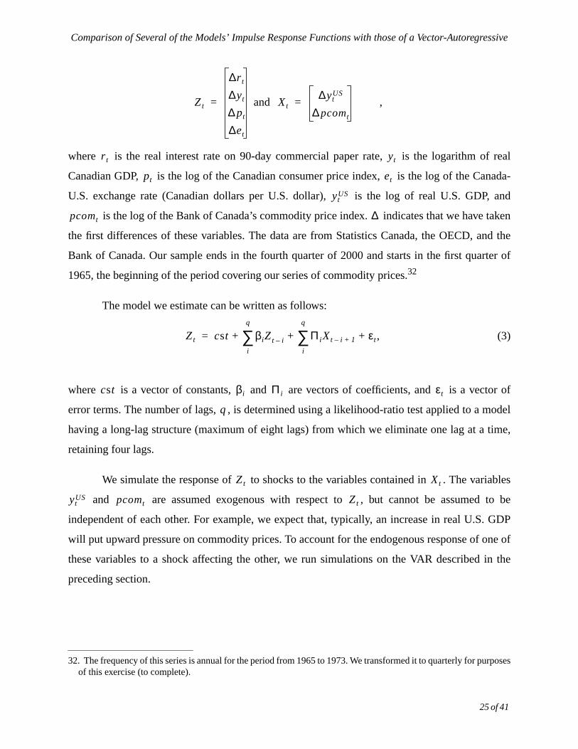
where is the real interest rate on 90-day commercial paper rate, is the logarithm o

Canadian GDP, is the log of the Canadian consumer price index, is the log of the Ca

U.S. exchange rate (Canadian dollars per U.S. dollar), is the log of real U.S. GDP

is the log of the Bank of Canada’s commodity price index. indicates that we have t

the first differences of these variables. The data are from Statistics Canada, the OECD, a

Bank of Canada. Our sample ends in the fourth quarter of 2000 and starts in the first qua

1965, the beginning of the period covering our series of commodity prices.32

The model we estimate can be written as follows:

, (3)

where is a vector of constants, and are vectors of coefficients, and is a vect

error terms. The number of lags, , is determined using a likelihood-ratio test applied to a m

having a long-lag structure (maximum of eight lags) from which we eliminate one lag at a t

retaining four lags.

We simulate the response of to shocks to the variables contained in . The vari

and are assumed exogenous with respect to , but cannot be assumed

independent of each other. For example, we expect that, typically, an increase in real U.S

will put upward pressure on commodity prices. To account for the endogenous response of

these variables to a shock affecting the other, we run simulations on the VAR described

preceding section.

32. The frequency of this series is annual for the period from 1965 to 1973. We transformed it to quarterly for puof this exercise (to complete).

Zt

∆r t

∆yt

∆ pt

∆et

= Xt∆yt

US

∆ pcomt

=

r t yt

pt et

ytUS

pcomt ∆

Zt cst βiZt i– Πi Xt i– 1+ εt+i

q

∑+i

q

∑+=

cst βi Πi εt

q

Zt Xt

ytUS pcomt Zt

25 of 41

Comparison of Several of the Models’ Impulse Response Functions with those of a Vector-Autoregressive

erate a

s using

ation

cond,

adian

. For

may

hird,

at our

d.

odity

rious

ence

r cent,

s the

rt-term

l U.S.

VAR

S,

t the

ed to

becausepositive

These shocks are of the same magnitude as those run with the other models. We gen

95 per cent confidence interval around the VAR’s estimated responses to the various shock

bootstrapping-type simulations.

Our approach has several limitations. First, even though the VAR is a good approxim

of the historical relationship between the affected variables, it remains an approximation. Se

while it is calibrated to closely reflect the importance of the various components to the Can

economy, the commodity price index we use may differ from that used in the other models

example, some models contain several prices, or price indexes, for commodities, which

appear in different equations. The shock to real U.S. GDP is not affected by this problem. T

we consider only two types of shocks and three variables in the comparison. It is possible th

conclusions would have been different had other shocks and other variables been examine

Figures 1.2 and 1.3 in Appendix 2 compare the impact of real U.S. GDP and comm

price shocks on real GDP, CPI inflation, and the Canadian exchange rate in the va

participating models with the corresponding responses from the VAR model. The confid

interval associated with the VAR is indicated with the red dashed line.33

i.) A temporary external shock

Real U.S. GDP is increased by 1 per cent, 0.75 per cent, 0.50 per cent, and 0.25 pe

respectively, during the first four quarters. Note that this temporary shock incorporate

endogenous response of some U.S. macroeconomic variables, such as inflation and sho

interest rates, as well as the endogenous response of commodity prices.

An interesting observation about the reaction of real Canadian GDP to a shock to rea

GDP is that it is often smaller, in the very short run, in the participating models than in the

model. In particular, it responds much less in the CEFM, M1-VECM, MULTIMOD, FOCU

FOCUS-CE and WEFA models than in the VAR model. It is also interesting to note tha

NAOMI model (in the short term) and QPM overestimate the response of inflation compar

the VAR and other models.

33. In the case of a positive shock, the QPM model response is biased upwards compared to the linear VARQPM has a non-linear aggregate supply curve. We therefore took an average of the model’s response to theand negative shocks.

26 of 41

Comparison of Several of the Models’ Impulse Response Functions with those of a Vector-Autoregressive

often

veral

For

of the

1-

the

GDP

ian

5 per

nitial

several

s that

ger

hort-

e in

ever,

s than

his

PM

ble.

tion of

t a

In several models the response of the exchange rate is quite different from, indeed

outside the (wide) estimated confidence interval of, that yielded by the VAR. Incidentally, se

models yield responses of a different sign from the VAR, especially in the short term.

example, while in the VAR, an increase in real U.S. GDP causes a short-term depreciation

Canadian dollar, the MTFM, MULTIMOD, both versions of the FOCUS model, WEFA, M

VECM, and INTERLINK models, predict the opposite. It is also interesting to note that, while

VAR predicts that the exchange rate should return to control following the temporary U.S.

shock, NAOMI, QPM, and INTERLINK predict large long-run depreciations of the Canad

dollar in response to that shock.

ii.) A temporary shock to commodity prices

During the first quarter, commodity prices increase 4 per cent, during the second 3.

cent, during the third 3 per cent, … , and during the eighth 0.5 per cent, returning to their i

value by the ninth quarter. Note that this shock incorporates the endogenous response of

U.S. macroeconomic variables, such as production, inflation, and short-term interest rates.

In several models, the response of real GDP to commodity price shocks resemble

generated by the VAR. MTFM, in the short term, and INTERLINK, in the short and the lon

term, differ most from the VAR. These two models are, in fact, the only ones to predict a s

term fall in production in Canada in response to a positive commodity price shock.

As in the case of the VAR, the response of inflation to this shock is generally positiv

the short term, except in the FOCUS model with backward-looking expectations. How

several models, especially the WEFA model and FOCUS-CE, show much stronger reaction

the VAR in the short term. The MULTIMOD and MTFM models are the closest to the VAR in t

respect.

We find great variation in our results for the exchange rate. DRI, INTERLINK, and Q

are particularly divergent from the VAR (and the other models) with respect to this varia

While the VAR predicts that an increase in commodity prices causes a short-term apprecia

the Canadian dollar, the DRI, MULTIMOD, CEFM, INTERLINK, and QPM models forecas

depreciation.34

27 of 41

Conclusions

sponse

f the

se this

ctions

es of

ks and

e, on

). The

core.

AR

els

my to

to the

del is

a few

ever,

and

spect

omy

under

urve

has onexportsrder to

We calculate a measure of the distance between the results generated by the re

functions of the participating models and the VAR—computed as the sum of squares o

differences between the impulse response functions of the models and the VAR. We then u

distance measure to rank the various models in terms of the distance of their response fun

from those of the VAR. Table 5 presents the results of these calculations for the two typ

shocks and the three variables we consider, along with an aggregate ranking over all shoc

variables. A minimum-rank criterion is used here. The model that is ranked first is the on

average, with the lowest score for the two shocks and three variables (each ranked equally

last-ranked model, i.e., that differing most from the VAR overall, is the one with the highest s

Our comparison of the models’ impulse response functions with those of a V

comprising very little economic structure reveal that the MTFM, NAOMI and CEFM mod

reflect relatively better than the other models the typical response of the Canadian econo

shocks to real U.S. GDP and to commodity prices. Some models yield results that are close

VAR for certain variables and certain shocks, but are much further in other cases. No mo

among the closest to the VAR for all variables and all shocks. Every model contains at least

impulse response functions that diverge significantly from those estimated by the VAR. How

the responses generated by the MTFM are closest to the VAR overall followed by NAOMI

CEFM, and those from M1-VECM, DRI and INTERLINK, the furthest.

5. Conclusions

This report examines and compares twelve models of the Canadian economy with re

to their paradigm, structure and dynamics properties. Although they are all “open econ

models”, the models are nevertheless quite different. The twelve models can be classified

two economic paradigms. The first one is the “conventional” paradigm (or the Phillips-c

paradigm) and the second one is the “money matters” paradigm.

34. The endogenous response of real U.S. GDP to the commodity price shock partially explains the effect itthe exchange rate in QPM. Indeed, real U.S. GDP tends to decline in response to this shock, reducing ourto the United States. To maintain foreign debt at a constant level, the Canadian dollar must depreciate in ostimulate Canadian exports.

28 of 41

Conclusions

ction

rket,

are

ts in

oney

and -

tion

ce of

six

-

lays

in the

the

rices.

ons:

-CE,

e

sistent

del-

etary

ffect

wing

d

cy

etary

Under the conventional paradigm, inflation is determined by price adjustments in rea

to inflation expectations and by factor disequilibrium in various markets (e.g., the labour ma

the goods market). While most models fall under the “conventional” paradigm, there

nevertheless important differences within this paradigm.

Under the “money matters” paradigm, inflation is mostly determined by movemen

monetary aggregates. Two models fall under this category: the M1-VECM in which the m

gap - the disequilibrium between money supply and estimated long-term money dem

influences inflation, while still allowing a role for the output gap, and the Limited Participa

Model (henceforth LPM), in which rigidities in adjusting money balances are the main sour

the short-run non-neutrality of monetary policy.

Within the conventional paradigm, inflation is determined by a linear Phillips curve in

participating models: CEFM, DRI, FOCUS, INTERLINK, WEFA and NAOMI. While the M1

VECM falls under the “money matters” paradigm, the disequilibrium in the product market p

also a role in the adjustment of prices. Asymmetries in the inflation process are introduced

models of FOCUS-CE, MULTIMOD and QPM. On the other hand, the MTFM model of

Conference Board uses a very disaggregated approach to determining the adjustment of p

Eight out of twelve models assume purely backward-looking inflation expectati

CEFM, DRI, FOCUS, INTERLINK, MTFM, WEFA, M1-VECM, and NAOMI while the

following three models also impute model-consistent inflation expectations to them: FOCUS

MULTIMOD, and QPM. In QPM and MULTIMOD, in particular, the hybrid Phillips curv

assigns more weight to backward-looking inflation expectations as compared to model-con

inflation expectations. The LPM is the only calibrated model which incorporates purely mo

consistent behaviour and is optimally derived from microfoundations.

The models can be also differentiated based on the channels through which mon

policy actions affect the economy. In most participating models, monetary policy actions a

the economy through the level of short-term interest rates. This is the case of the follo

models: CEFM, DRI, FOCUS, FOCUS-CE, INTERLINK, MTFM, WEFA, LPM an

MULTIMOD. In other models, such in the M1-VECM, NAOMI and QPM, the monetary poli

transmission mechanism works through the slope of the yield curve. In all models, mon

29 of 41

Conclusions

nd/or

ility.

I is a

nd is

adian

e have

etary

ndard

f the

ck in

ing

EFM

nomy

least a

policy affects the real economy in the short run because of nominal rigidities (wages a

prices, money balances for LPM), but remains neutral in the long term owing to price flexib

Finally, there are also differences in estimation techniques and sizes. For example, NAOM

small estimated model while QPM is a large-scale calibrated model. MTFM, on the other ha

a fairly disaggregated model compared to most of the other models.

To further understand the structure and properties of the twelve models of the Can

economy, i.e., the way the various models respond to different macroeconomic shocks, w

examined the dynamic properties of the various models when they use a simple mon

authority reaction function, such as the one proposed by John Taylor (1993). The eight sta

shocks considered in our study reveal significant differences in the dynamic properties o

participating models. However, we would expect that similar models react to the same sho

the same way—yet that is not what we observe.

Finally, our comparison of the models’ reaction functions with those of a VAR compris

very little economic structure suggests that some models, especially MTFM, NAOMI and C

do a slightly better job than the others of reflecting the typical response of the Canadian eco

to shocks to real U.S. GDP and to commodity prices. Nonetheless, every model contains at

few reaction functions that diverge significantly from those estimated by the VAR.

30 of 41

and

Bank

ing

Bankwa:

oft No.

f the

and

omy.”

y?”

k of

ODtary

licy

ian

References

Adam, C. and S. Hendry. 2000. “The M1 Vector-Error-Correction Model: Some ExtensionsApplications.” In Money, Monetary Policy, and Transmission Mechanisms, 151–80.Proceedings of a conference held by the Bank of Canada, November 1999. Ottawa:of Canada

Armour, J, B. Fung and D. Maclean, “Taylor Rules in the Quarterly Projection Model,” WorkPaper 2002-1, Bank of Canada.

Black, R, D. Laxton, D. Rose, and R. Tetlow. 1994. “The Steady-State Model: SSQPM, Theof Canada’s New Quarterly Projection Model, Part 1,” Technical Report No. 72. OttaBank of Canada.

Blanchard, O.J. 1985. “Debt, Deficits, and Finite Horizons.”Journal of Political Economy93(April): 223–46.

Buiter, W.H. 1988. “Death, Birth, Productivity Growth and Debt Neutrality.”The EconomicJournal 98 (391): 279–93.

Coletti, D., B. Hunt, D. Rose, and R. Tetlow. 1996. “The Dynamic Model: QPM, The BankCanada’s New Quarterly Projection Model, Part 3,” Bank of Canada Technical Repor75.

Côté, D. and J.-P. Lam, “Simple Rules in the M1-VECM,” presented at the 2001 meeting oCanadian Economic Association at McGill University (Montréal).

DeSerres, A., B. Robidoux, and B.-S. Wong. 1998. “CEFM96: Part 2, Dynamic ForecastingSimulation Properties,” July 1998, Working Paper 98–06.

Dungan, P. 1997. “Quarterly Forecasting and User Simulation Model of the Canadian EconInstitute for Policy Analysis, University of Toronto.

Hendry, Scott (1995) "Long-Run Demand for M1", Bank of Canada Working Paper 95-11.

Hendry, Ho, and Moran, 2001. “Policy Rules in Limited Participation Models.”

Hetzel, Robert L., The Taylor Rule: Is it a Useful Guide to Understanding Monetary PolicFederal Reserve Bank of RichmondQuarterly Review, Volume 86, No. 2, 2000.

Kozicki, Sharon, “How Useful are Taylor Rules for Monetary Policy,” Federal Reserve BanKansas CityEconomic Review, 1999.

Laxton Douglas, Peter Isard, Hamid Faruqee, Eswar Prasad and Bart Turtelboom, “MULTIMMark III: The Core Dynamic and Steady-State Models,” 1998, International MoneFund Occasional Paper No. 164.

Levin, Andrew, Volker Wieland and John C. Williams, “Robustness of Simple Monetary PoRules under Model Uncertainty,” in John B. Taylor, ed.,Monetary Policy Rules, Chicago:University of Chicago Press, 1999, 263-299.

Murchison, Stephen, “A New Quarterly Forecasting Model Part II: A Guide to CanadNAOMI,” Dept of Finance Working Paper 2001-25.

31 of 41

s to

el.”

ing

olicy

e

r the

O’Reilly, B, G. Paulin, and P. Smith. 1983. “Responses of Various Econometric ModelSelected Policy Shocks,” Technical Report No. 38. Ottawa: Bank of Canada.

Richardson, P. 1988. “The Structure and Simulation Properties of OECD’s INTERLINK ModOECD Economic Studies, No. 10, Spring.

Robidoux, B. and B.-S. Wong. 1998. “CEFM96: Part 1, Model Structure,” July 1998. WorkPaper 98–05.

Sims Chris, “A Review of Monetary Policy Rules, John B. Taylor, ed.,”Journal of EconomicLiterature, 2001, 39(2).

Svensson, Lars E.O., “Inflation Targeting as a Monetary Policy Rule,”Journal of MonetaryEconomics, 1999, 43, 607-654

Svensson, Lars E.O., “Open-Economy Inflation Targeting,”Journal of International Economics,2000, 50(1), 155-83.

Svensson, Lars E.O, “What Is Wrong with Taylor Rules? Using Judgment in Monetary PThrough Targeting Rules,” 2001, Working Paper.

Taylor, John B., “Discretion Versus Policy Rules in Practice,”Canergie-Rochester ConferencSeries on Public Policy, 1993, 39, 195-214.

Taylor, John B, “The Robustness and Efficiency of Monetary Policy Rules as Guidelines foECB,” European Economic Review, 1999.

Taylor, John B, “The Role of the Exchange Rate in Monetary Policy Rules,”The AmericanEconomic Review, 2001, 91.

Weil, P. 1989. “Overlapping Families of Infinitely-Lived Agents.”Journal of Public Economics38 (March): 183–98.

32 of 41

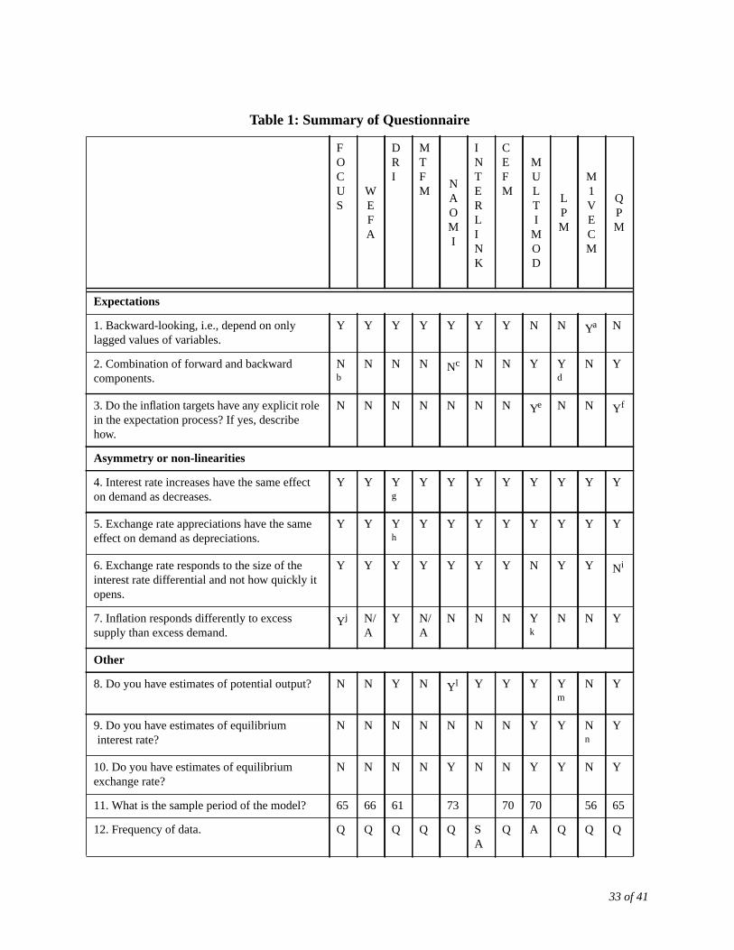
Table 1: Summary of Questionnaire

FOCUS

WEFA

DRI

MTFM

NAOMI

INTERLINK

CEFM

MULTI

MOD

LPM

M1VECM

QPM

Expectations

1. Backward-looking, i.e., depend on onlylagged values of variables.

Y Y Y Y Y Y Y N N Ya N

2. Combination of forward and backwardcomponents.

Nb

N N N Nc N N Y Yd

N Y

3. Do the inflation targets have any explicit rolein the expectation process? If yes, describehow.

N N N N N N N Ye N N Yf

Asymmetry or non-linearities

4. Interest rate increases have the same effecton demand as decreases.

Y Y Yg

Y Y Y Y Y Y Y Y

5. Exchange rate appreciations have the sameeffect on demand as depreciations.

Y Y Yh

Y Y Y Y Y Y Y Y

6. Exchange rate responds to the size of theinterest rate differential and not how quickly itopens.

Y Y Y Y Y Y Y N Y Y Ni

7. Inflation responds differently to excesssupply than excess demand.

Yj N/A

Y N/A

N N N Yk

N N Y

Other

8. Do you have estimates of potential output? N N Y N Yl Y Y Y Ym

N Y

9. Do you have estimates of equilibriuminterest rate?

N N N N N N N Y Y Nn

Y

10. Do you have estimates of equilibriumexchange rate?

N N N N Y N N Y Y N Y

11. What is the sample period of the model? 65 66 61 73 70 70 56 65

12. Frequency of data. Q Q Q Q Q SA

Q A Q Q Q

33 of 41

a. The money gap, however, is supposed to bring some forward-looking dimension to the model.b. Consistent expectation version.c. Monetary policy is forward-looking.d. Model-consistent expectations only.e. No explicit role in expectations other than through the weight on the model-consistent lead of inflation

in the expectation process.f. Forward-looking expectations are model-consistent. If monetary authorities achieve target, then this is

taken into account.g. Small changes have similar effects. The biggest non-linearities occur when economy is in an excess

demand position.h. Small changes have similar effects. The biggest non-linearities occur when economy is in an excess

demand position.i. Uncovered interest differential is the driving effect, so persistence of gap matters. Also, expected future

pfx has a backward-looking component.pfxt - Et(pfxt+1) = 0.25[i* – i]j. Phillips curve is non-linear in usual form.k. Phillips curve is non-linear.l. Potential output is exogenous to model.m. For 8, 9, and 10, use either steady-state values or values arising in a model with no nominal rigidities.n. A steady-state value is imposed.

34 of 41

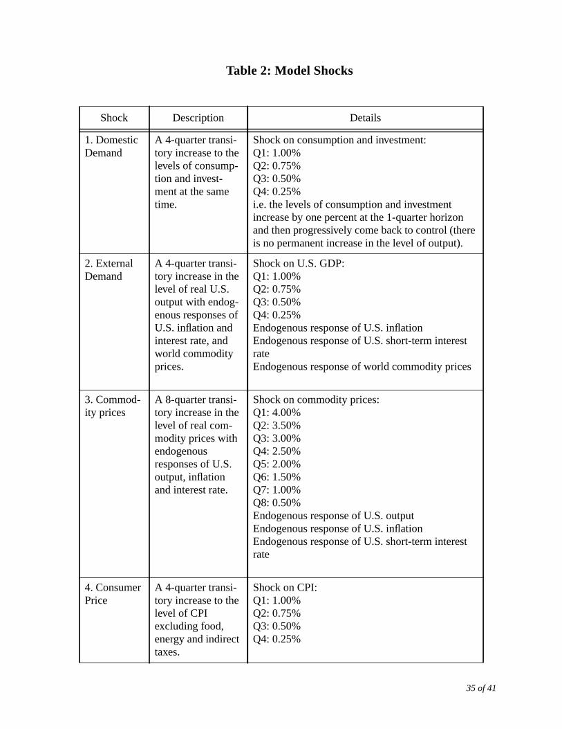
Table 2: Model Shocks

Shock Description Details

1. DomesticDemand

A 4-quarter transi-tory increase to thelevels of consump-tion and invest-ment at the sametime.

Shock on consumption and investment:Q1: 1.00%Q2: 0.75%Q3: 0.50%Q4: 0.25%i.e. the levels of consumption and investmentincrease by one percent at the 1-quarter horizonand then progressively come back to control (thereis no permanent increase in the level of output).

2. ExternalDemand

A 4-quarter transi-tory increase in thelevel of real U.S.output with endog-enous responses ofU.S. inflation andinterest rate, andworld commodityprices.

Shock on U.S. GDP:Q1: 1.00%Q2: 0.75%Q3: 0.50%Q4: 0.25%Endogenous response of U.S. inflationEndogenous response of U.S. short-term interestrateEndogenous response of world commodity prices

3. Commod-ity prices

A 8-quarter transi-tory increase in thelevel of real com-modity prices withendogenousresponses of U.S.output, inflationand interest rate.

Shock on commodity prices:Q1: 4.00%Q2: 3.50%Q3: 3.00%Q4: 2.50%Q5: 2.00%Q6: 1.50%Q7: 1.00%Q8: 0.50%Endogenous response of U.S. outputEndogenous response of U.S. inflationEndogenous response of U.S. short-term interestrate

4. ConsumerPrice

A 4-quarter transi-tory increase to thelevel of CPIexcluding food,energy and indirecttaxes.

Shock on CPI:Q1: 1.00%Q2: 0.75%Q3: 0.50%Q4: 0.25%

35 of 41

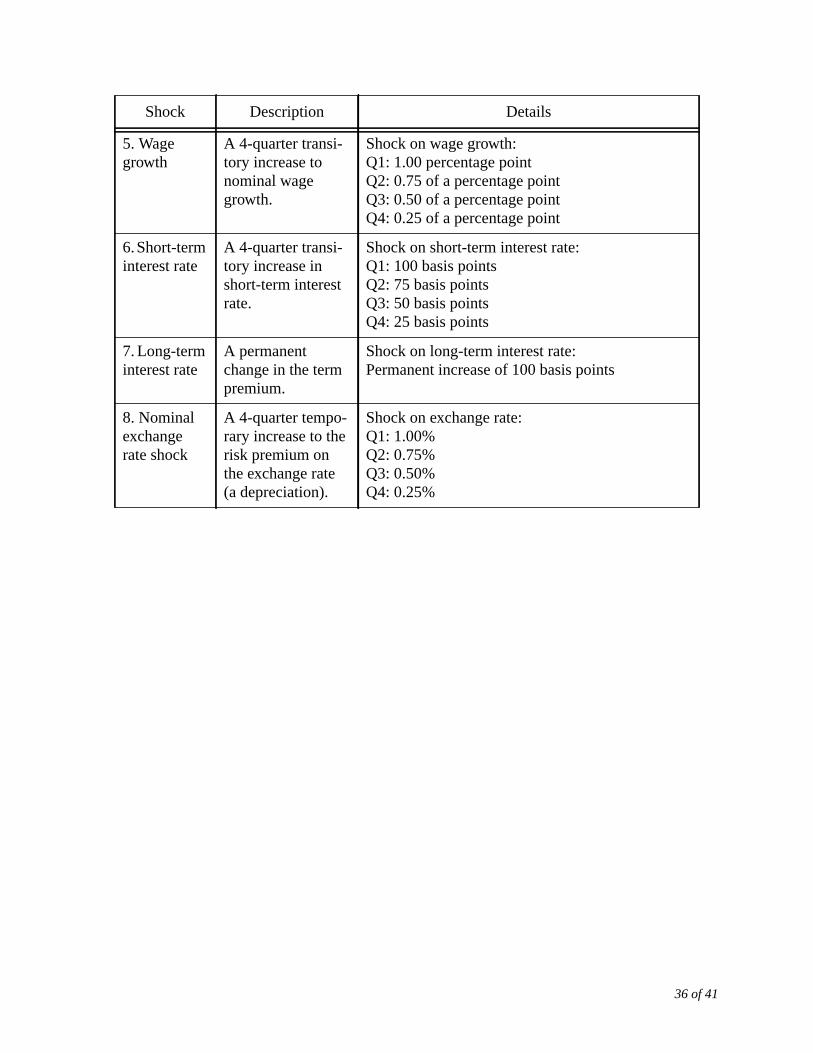
5. Wagegrowth

A 4-quarter transi-tory increase tonominal wagegrowth.

Shock on wage growth:Q1: 1.00 percentage pointQ2: 0.75 of a percentage pointQ3: 0.50 of a percentage pointQ4: 0.25 of a percentage point

6.Short-terminterest rate

A 4-quarter transi-tory increase inshort-term interestrate.

Shock on short-term interest rate:Q1: 100 basis pointsQ2: 75 basis pointsQ3: 50 basis pointsQ4: 25 basis points

7. Long-terminterest rate

A permanentchange in the termpremium.

Shock on long-term interest rate:Permanent increase of 100 basis points

8. Nominalexchangerate shock

A 4-quarter tempo-rary increase to therisk premium onthe exchange rate(a depreciation).

Shock on exchange rate:Q1: 1.00%Q2: 0.75%Q3: 0.50%Q4: 0.25%

Shock Description Details

36 of 41

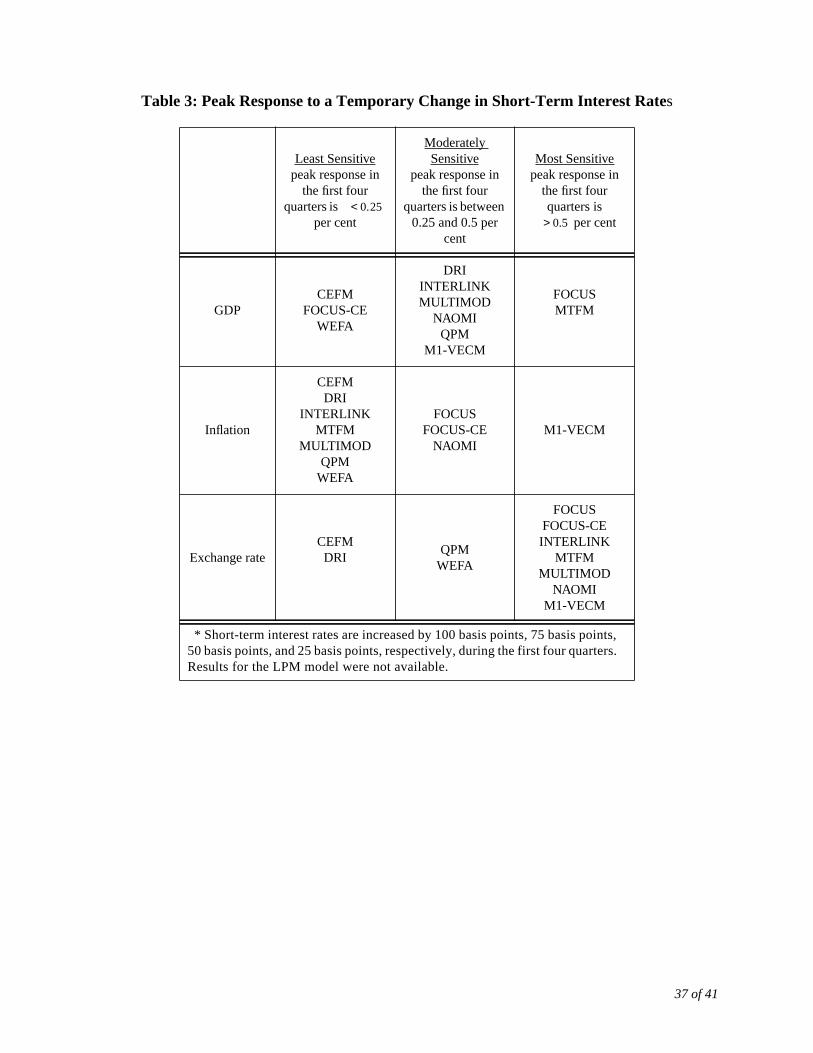
Table 3: Peak Response to a Temporary Change in Short-Term Interest Rates

Least Sensitivepeak response in

the first fourquarters is

per cent

ModeratelySensitive

peak response inthe first four

quarters is between0.25 and 0.5 per

cent

Most Sensitivepeak response in

the first fourquarters is

per cent

GDPCEFM

FOCUS-CEWEFA

DRIINTERLINKMULTIMOD

NAOMIQPM

M1-VECM

FOCUSMTFM

Inflation

CEFMDRI

INTERLINKMTFM

MULTIMODQPM

WEFA

FOCUSFOCUS-CE

NAOMIM1-VECM

Exchange rateCEFMDRI

QPMWEFA

FOCUSFOCUS-CEINTERLINK

MTFMMULTIMOD

NAOMIM1-VECM

* Short-term interest rates are increased by 100 basis points, 75 basis points,50 basis points, and 25 basis points, respectively, during the first four quarters.Results for the LPM model were not available.

0.25<0.5>

37 of 41

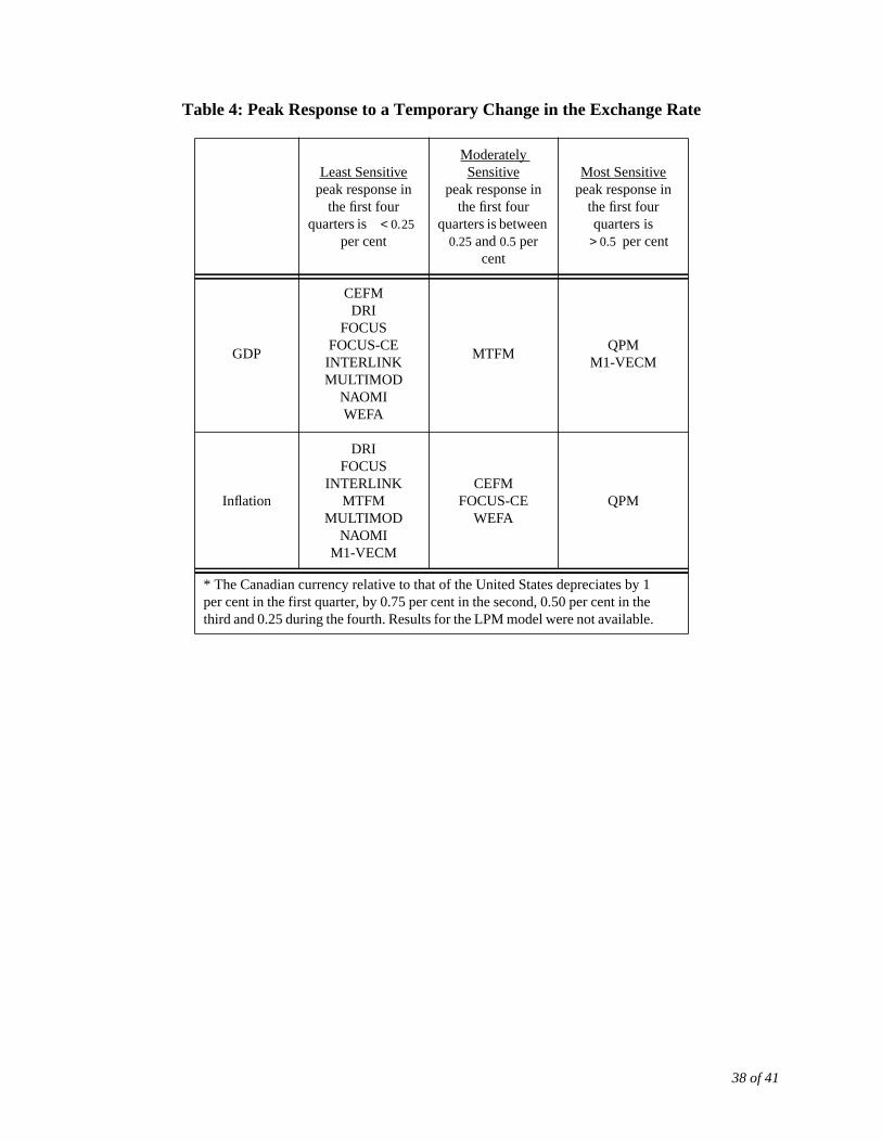
Table 4: Peak Response to a Temporary Change in the Exchange Rate

Least Sensitivepeak response in

the first fourquarters is

per cent

ModeratelySensitive

peak response inthe first four

quarters is between0.25 and0.5 per

cent

Most Sensitivepeak response in

the first fourquarters is

per cent

GDP

CEFMDRI

FOCUSFOCUS-CEINTERLINKMULTIMOD

NAOMIWEFA

MTFMQPM

M1-VECM

Inflation

DRIFOCUS

INTERLINKMTFM

MULTIMODNAOMI

M1-VECM

CEFMFOCUS-CE

WEFAQPM

* The Canadian currency relative to that of the United States depreciates by 1per cent in the first quarter, by 0.75 per cent in the second, 0.50 per cent in thethird and 0.25 during the fourth. Results for the LPM model were not available.

0.25<0.5>

38 of 41

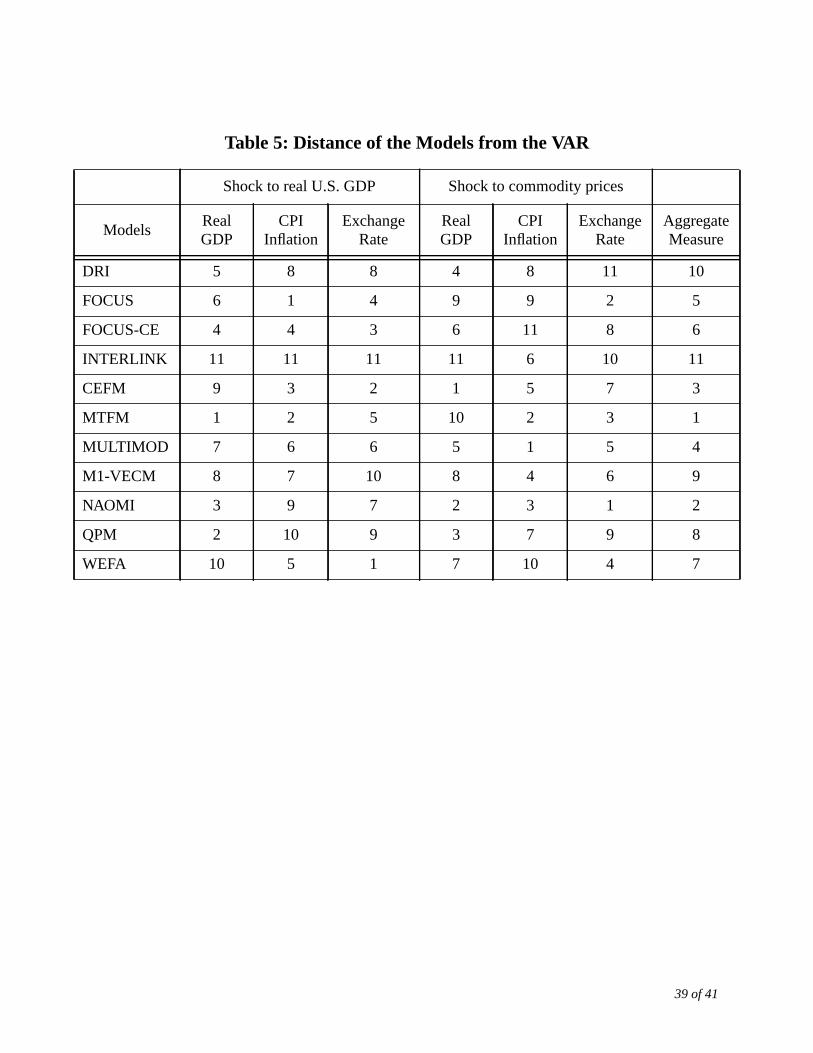
D

F

F

I

C

M

M

M

N

Q

W

Table 5: Distance of the Models from the VAR

Shock to real U.S. GDP Shock to commodity prices

ModelsRealGDP

CPIInflation

ExchangeRate

RealGDP

CPIInflation

ExchangeRate

AggregateMeasure

RI 5 8 8 4 8 11 10

OCUS 6 1 4 9 9 2 5

OCUS-CE 4 4 3 6 11 8 6

NTERLINK 11 11 11 11 6 10 11

EFM 9 3 2 1 5 7 3

TFM 1 2 5 10 2 3 1

ULTIMOD 7 6 6 5 1 5 4

1-VECM 8 7 10 8 4 6 9

AOMI 3 9 7 2 3 1 2

PM 2 10 9 3 7 9 8

EFA 10 5 1 7 10 4 7

39 of 41

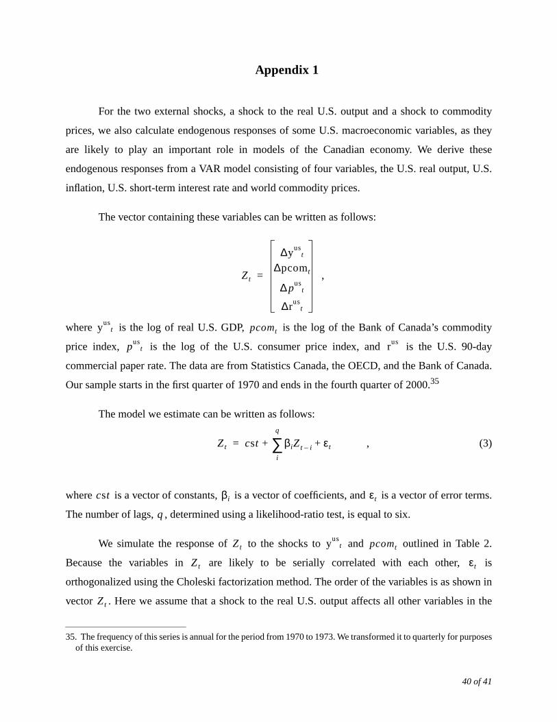
odity

as they

hese

t, U.S.

dity

-day

anada.

rms.

e 2.

is

wn in

in the

rposes

Appendix 1

For the two external shocks, a shock to the real U.S. output and a shock to comm

prices, we also calculate endogenous responses of some U.S. macroeconomic variables,

are likely to play an important role in models of the Canadian economy. We derive t

endogenous responses from a VAR model consisting of four variables, the U.S. real outpu

inflation, U.S. short-term interest rate and world commodity prices.

The vector containing these variables can be written as follows:

,

where is the log of real U.S. GDP, is the log of the Bank of Canada’s commo

price index, is the log of the U.S. consumer price index, and is the U.S. 90

commercial paper rate. The data are from Statistics Canada, the OECD, and the Bank of C

Our sample starts in the first quarter of 1970 and ends in the fourth quarter of 2000.35

The model we estimate can be written as follows:

, (3)

where is a vector of constants, is a vector of coefficients, and is a vector of error te

The number of lags, , determined using a likelihood-ratio test, is equal to six.

We simulate the response of to the shocks to and outlined in Tabl

Because the variables in are likely to be serially correlated with each other,

orthogonalized using the Choleski factorization method. The order of the variables is as sho

vector . Here we assume that a shock to the real U.S. output affects all other variables

35. The frequency of this series is annual for the period from 1970 to 1973. We transformed it to quarterly for puof this exercise.

Zt

∆yust

∆pcomt

∆ pust

∆rust

=

yust pcomt

pust rus

Zt cst βiZt i– εt+i

q

∑+=

cst βi εt

q

Zt yust pcomt

Zt εt

Zt

40 of 41

next

same period, while a shock to the world commodity prices only affects the U.S. output in the

period.

41 of 41