Macroeconomic Modeling for Monetary Policy Evaluation · Macroeconomic Modeling for Monetary Policy Evaluation ... term has probably become the most popular, ... These movements in

Macroeconomic Modeling for MonetaryPolicy Evaluation

Jordi Galı and Mark Gertler

Q uantitative macroeconomic modeling fell out of favor during the 1970sfor two related reasons: First, some of the existing models, like theWharton econometric model and the Brookings model, failed spectac-ularly to forecast the stagflation of the 1970s. Second, leading macro-

economists leveled harsh criticisms of these frameworks. Lucas (1976) and Sargent(1981), for example, argued that the absence of an optimization-based approach tothe development of the structural equations meant that the estimated modelcoefficients were likely not invariant to shifts in policy regimes or other types ofstructural changes. Similarly, Sims (1980) argued that the absence of convincingidentifying assumptions to sort out the vast simultaneity among macroeconomicvariables meant that one could have little confidence that the parameter estimateswould be stable across different regimes. These powerful critiques clarified whyeconometric models fit largely on statistical relationships from a previous era didnot survive the structural changes of the 1970s.

In the 1980s and 1990s, many central banks continued to use reduced-formstatistical models to produce forecasts of the economy that presumed no structuralchange, but they did so knowing that these models could not be used with anydegree of confidence to predict the outcome of policy changes. Thus, monetarypolicymakers turned to a combination of instinct, judgment, and raw hunches to

y Jordi Galı is the Director of the Centre de Recerca en Economia Internacional (CREI) andProfessor of Economics, Universitat Pompeu Fabra, both in Barcelona, Spain. Mark Gertler isHenry and Lucy Moses Professor of Economics, New York University, New York City, NewYork. Their e-mail addresses are �[email protected]� and �[email protected]�, respectively.

Journal of Economic Perspectives—Volume 21, Number 4—Fall 2007—Pages 25–45

assess the implications of different policy paths for the economy. Within the lastdecade, however, quantitative macroeconomic frameworks for monetary policyevaluation have made a comeback. What facilitated the development of theseframeworks were two independent literatures that emerged in response to thedownfall of traditional macroeconomic modeling: New Keynesian theory and realbusiness cycle theory. The New Keynesian paradigm arose in the 1980s as anattempt to provide microfoundations for key Keynesian concepts such as theinefficiency of aggregate fluctuations, nominal price stickiness, and the non-neu-trality of money (for discussion and references, see Mankiw and Romer, 1991). Themodels of this literature, however, were typically static and designed mainly forqualitative as opposed to quantitative analysis. By contrast, real business cycletheory, which was developing concurrently, demonstrated how it was possible tobuild quantitative macroeconomic models exclusively from the “bottom up”—thatis, from explicit optimizing behavior at the individual level (Prescott, 1986). Thesemodels, however, abstracted from monetary and financial factors and thus couldnot address the issues that we just described. In this context, the new frameworksreflect a natural synthesis of the New Keynesian and real business cycle approaches.

Overall, the progress has been remarkable. A decade ago it would have beenunimaginable that a tightly structured macroeconometric model would have muchhope of capturing real-world data, let alone of being of any use in the monetarypolicy process. However, frameworks have been recently developed that forecast aswell as the reduced-form models of an earlier era (for example, Christiano, Eichen-baum, and Evans, 2005; Smets and Wouters, 2003, 2007). Because these modelshave explicit theoretical foundations, they can also be used for counterfactualpolicy experiments. A tell-tale sign that these frameworks have crossed a criticalthreshold for credibility is their widespread use at central banks across the globe.While these models are nowhere close to removing the informal dimension of themonetary policy process, they are injecting an increased discipline to thinking andcommunication about monetary policy.

To be sure, there were some important developments in between the tradi-tional macroeconometric models and the most recent vintage. Frameworks such asTaylor (1979) and Fuhrer and Moore (1995) incorporated several importantfeatures that were missing from the earlier vintage of models: 1) the Phelps/Friedman natural rate hypothesis of no long-run tradeoff between inflation andunemployment, and 2) rational formation of expectations. At the same time,however, the structural relations of these models typically did not evolve fromindividual optimization. The net effect was to make these frameworks susceptible tosome of the same criticisms that led to the demise of the earlier generation ofmodels (for example, Sargent, 1981). It is also relevant that over the last 20 yearsthere have been significant advances in dynamic optimization and dynamic generalequilibrium theory. To communicate with the profession at large, particularly theyounger generations of scholars, it was perhaps ultimately necessary to develop

26 Journal of Economic Perspectives

applied macroeconomic models using the same tools and techniques that havebecome standard in modern economic analysis.

Overall, our goal in this paper is to describe the main elements of this newvintage of macroeconomic models. Among other things, we describe the keydifferences with respect to the earlier generation of macro models. In doing so, wehighlight the insights for policy that these new frameworks have to offer. Inparticular, we will emphasize two key implications of these new frameworks.

1. Monetary transmission depends critically on private sector expectations of the futurepath of the central bank’s policy instrument, the short-term interest rate. Ever since therational expectations revolution, it has been well understood that the effects ofmonetary policy depend on private sector expectations. This early literature, how-ever, typically studied how expectations formation influenced the effect of acontemporaneous shift in the money supply on real versus nominal variables (forexample, Fischer, 1977; Taylor, 1980). In this regard, the new literature differs intwo important ways. First, as we discuss below, it recognizes that central bankstypically employ a short-term interest rate as the policy instrument. Second, withinthe model, expectations of the future performance of the economy enter thestructural equations, since these aggregate relations are built on forward-lookingdecisions by individual households and firms. As a consequence, the current valuesof aggregate output and inflation depend not only on the central bank’s currentchoice of the short-term interest rate, but also on the anticipated future path of thisinstrument. The practical implication is that how well the central bank is able tomanage private sector expectations about its future policy settings has importantconsequences for its overall effectiveness. Put differently, in these paradigms thepolicy process is as much, if not more, about communicating the future intentionsof policy in a transparent way, as it is about choosing the current policy instrument.In this respect, these models provide a clear rationale for the movement towardgreater transparency in intentions that central banks around the globe appear to bepursuing.

2. The natural (flexible price equilibrium) values of both output and the real interest rateprovide important reference points for monetary policy—and may fluctuate considerably.While nominal rigidities are introduced in these new models in a more rigorousmanner than was done previously, it remains true that one can define natural valuesfor output and the real interest rate that would arise in equilibrium if these frictionswere absent. These natural values provide important benchmarks, in part becausethey reflect the (constrained) efficient level of economic activity and also in partbecause monetary policy cannot create persistent departures from the naturalvalues without inducing either inflationary or deflationary pressures. Within tradi-tional frameworks, the natural levels of output and the real interest rate aretypically modeled as smoothed trends. Within the new frameworks they are mod-eled explicitly. Indeed, roughly speaking, they correspond to the values of outputand the real interest rate that a frictionless real business cycle model wouldgenerate, given the assumed preferences and technology. As real business cycle

Jordi Galı and Mark Gertler 27

theory suggests, further, these natural levels can vary considerably, given that theeconomy is continually buffeted by “real” shocks including oil price shocks, shifts inthe pace of technological change, tax changes, and so on. Thus, these new modelsidentify an important challenge for central banks: that of tracking the naturalequilibrium of the economy, which is not directly observable.

In the next section, we lay out a canonical baseline model that captures the keyfeatures of the new macro models and we draw out the corresponding insights formonetary policy. We then discuss some of the policy issues brought by the newmodels. We conclude by discussing some modifications of the baseline model thatare necessary to take it to data, as well as other extensions designed to improve itsrealism.

A Baseline Model

In this section we lay out a baseline framework that captures the keyfeatures of the new vintage macro models and is useful for qualitative analysis.The specific framework we develop is a variant of the canonical model discussedin Goodfriend and King (1997), Clarida, Galı, and Gertler (1999), Woodford(2003), and Galı (forthcoming), among others, but is modified to allow forinvestment.1 As with the real business cycle paradigm, the starting point is astochastic dynamic general equilibrium model. More specifically, it is a stochas-tic version of the conventional neoclassical growth model, modified to allow forvariable labor supply.2 As we suggested above, to make the framework suit-able for monetary policy analysis, it is necessary not only to introducenominal variables explicitly, but also some form of nominal stickiness. In thisregard, three key ingredients that are prominent features of the New Keynesianparadigm are added to the frictionless real business cycle model: money,monopolistic competition, and nominal rigidities. We briefly discuss each inturn.

The key role of money emphasized in the new monetary models is its functionas a unit of account—that is, as the unit in which the prices of goods and assets arequoted. The existence of money thus gives rise to nominal prices. It is important,

1 We have avoided a label for the new frameworks because a variety have been used. Goodfriend andKing employ the term “New Neoclassical Synthesis,” while Woodford uses “NeoWicksellian.” At theinsistence of a referee, in our 1999 paper with Richard Clarida, we used “New Keynesian.” The latterterm has probably become the most popular, though it does not adequately reflect the influence of realbusiness cycle theory.2 We note that the real business cycle model treats shocks to total factor productivity as the main drivingforce of business cycles. By contrast, estimated versions of the new monetary models suggest thatintertemporal disturbances (that is, shocks to either consumption or investment spending) are key. See,for example, Galı and Rabanal (2005), Smets and Wouters (2007), or Primiceri, Schaumberg, andTambalotti (2006).


however, to distinguish between money and monetary policy: Monetary policyaffects real activity in the short run purely through its effect on market interestrates. In particular, the central bank affects aggregate spending by controlling theshort-term interest rate and, through market expectations of its future short ratedecisions, by influencing the full yield curve. To control the short-term interestrate, the central bank adjusts the money supply to accommodate the demand formoney at the desired interest rate. These movements in the money supply, how-ever, exert no independent effect on aggregate demand. Because real moneybalances are a negligible component of total wealth, the models are designed in away that abstracts from wealth effects of money on spending. Thus, while monetarypolicy is central in these models, money per se plays no role other than to providea unit of account.

To introduce price stickiness in a rigorous way, firms must be price setters asopposed to price takers. For this reason, it is necessary to introduce some form ofimperfect competition, where firms face downward-sloping demand curves and,thus, a meaningful price-setting decision. This can be accomplished in a straight-forward way with a version of the Dixit and Stiglitz (1977) model of monopolisticcompetition in which each firm produces a differentiated good and sets the pricefor the good while taking as given all aggregate variables, and this approach hasgenerally been adopted by the new frameworks.

As with traditional models, what ultimately permits monetary policy to haveleverage over the real economy in the short run is the existence of temporarynominal rigidities. Because nominal prices adjust sluggishly, by directly manipulat-ing nominal interest rates, the central bank is able to influence real rates and hencereal spending decisions, at least in the short run. The traditional models introducesluggish price adjustment by postulating a “Phillips curve” relating inflation tosome measure of excess demand, as well as lags of past inflation. By contrast, thesenew vintage models derive an inflation equation—often referred to as the NewKeynesian Phillips curve—explicitly from individual firms’ price-setting behavior,as we describe below.

We now turn to a description of our canonical framework. As with thetraditional framework, it is convenient to organize the system into three blocks:aggregate demand, aggregate supply, and policy. Further, it is possible to representeach subsector by a single equation. In an Appendix available with the onlineversion of this paper (at �http://www.e-jep.org�), we build up the aggregate de-mand and aggregate supply relationships in detail. In what follows, we present thecondensed aggregate demand and supply equations along with an informal moti-vation. By adding an additional relation that describes monetary policy, it is thenpossible to express the model as a three-equation system, similar in spirit to the waytraditional macroeconomic models have been represented. The main differencefrom the traditional framework, of course, is that the new vintage of models arebuilt on explicit micro foundations.

Macroeconomic Modeling for Monetary Policy Evaluation 29

Aggregate Demand/Supply: A Compact RepresentationIn developing this baseline model, it is useful to keep in mind that what

monetary policy can influence is the deviation of economic activity from its naturallevel. Within our baseline model, the natural level of economic activity is definedas the equilibrium that would arise if prices were perfectly flexible and all othercyclical distortions were absent. In the limiting case of perfect price flexibility,accordingly, the framework takes on the properties of a real business cycle model.One difference is that in the current framework, because there is monopolisticcompetition as opposed to perfect competition, the natural level of economicactivity is below the socially efficient level. However, this distinction does not affectthe nature of the associated cyclical dynamics of the natural level of economicactivity which, within our baseline framework, resemble those of a real businesscycle model with similar preferences and technology.

The aggregate demand relation is built up from the spending decisions of arepresentative household and a representative firm. In the baseline model, bothcapital and insurance markets are perfect. Within this frictionless setting, thehousehold satisfies exactly its optimizing condition for consumption/saving deci-sions. It thus adjusts its expected consumption growth positively to movements inthe expected real interest rate. Similarly, with perfect capital markets, the repre-sentative firm satisfies exactly its optimizing condition for investment: it variesinvestment proportionately with Tobin’s q, the ratio of the shadow value of installedcapital to the replacement value.

From the individual spending decisions, it is possible to derive an IS curve–typeequation that relates aggregate demand inversely to the short-term interest rate,similar in spirit to that arising in a traditional framework. In contrast to thetraditional model, however, expectations of the future value of the short-term ratematter as well. They do so by influencing long-term interest rates and asset prices.

In particular, let yt be the percentage gap between real output and its naturallevel, let rr t

l be the gap between the long-term real interest rate and its natural level,and let qt be the corresponding percentage gap in Tobin’s q.3 Then by takinglog-linear approximations of both the baseline model and the flexible price variant,it is possible to derive an aggregate demand equation that relates the output gap,yt, inversely to the real interest rate gap, rr t

l, and positively to the gap in Tobin’s q,qt, as follows:

yt � ��c�rr tl � �i�qt

3 To be clear, we define the natural level of economic activity in any given period to be period t,conditional on the beginning of period capital stock. Monetary policy has no effect on the natural levelof economic activity as we have defined it. Monetary policy can affect the path of the capital stock,though these effects are typically small in percentage terms under reasonable parameterizations of themodel.


where �c and �i are the shares of consumption and investment, respectively, insteady state output; � is the intertemporal elasticity of substitution; and � is theelasticity of the investment–capital ratio with respect to Tobin’s q. In effect, thisequation relates the output gap to the sum of two terms.

The first corresponds to the consumption gap and the second to the invest-ment gap. In particular, the consumption gap moves inversely with the long-termreal interest rate gap rr t

l . Intuitively, if the long-term real rate is above its naturalvalue, households will be induced to save more than in the natural equilibrium and,hence, consumption will be lower. Similarly, if q is above its natural value, firms willbe induced to invest more than they would under flexible prices.

To link aggregate demand to monetary policy, it is useful to define theshort-term real interest rate gap, rrt , as the difference between the short-term realrate and its natural equilibrium value, rrt

n, that is

rrt � �rt � Et�t�1� � rrtn

where rt is the short-term nominal interest rate and �t�1 is the rate of inflationfrom t to t � 1.

Two propositions follow from this relationship. The first proposition is that thelong-term real interest rate gap, rr t

l, depends positively on current and expectedfuture values of the short-term real interest rate gap, rrt . This proposition emergesfrom the link between long-term interest rates and current and expected short-terminterest rates implied by the expectation hypothesis of the term structure. Thesecond proposition is that the gap in Tobin’s q, qt , depends inversely on currentand expected future values of the short-term interest rate gap, rrt . This secondproposition arises because Tobin’s q depends on the discounted returns to capitalinvestment, where the discount rates depend on the expected path of short-termreal interest rates.

Thus, the mechanism through which monetary policy influences aggregatedemand can be thought of as working as follows: Given the sluggish adjustment ofprices, by varying the short-term nominal interest rate, the central bank is able toinfluence the short-term real interest rate and, hence, the corresponding realinterest rate gap. Through its current and expected future policy settings, thecentral bank is able to affect the corresponding path of rrt and, in turn, influencethe long-term real rate gap, rr t

l , and the gap in Tobin’s q, qt.As in the traditional models, the framework can incorporate exogenous fluc-

tuations in government purchases or other aggregate demand components. Thesefluctuations influence both the natural level of output and the natural real interestrate. However, the form of the aggregate demand equation is not affected, sincethis relation is expressed in terms of gap variables.

Finally, we note that the compact form of the aggregate demand curve de-pends on the assumption of perfect capital markets, so that both the permanent


income hypothesis for consumption and the q theory for investment are valid. As wediscuss later, recent work relaxes the assumption of perfect capital markets.

The aggregate supply relation evolves from the price-setting decisions of indi-vidual firms. To capture nominal price inertia, it is assumed that firms set prices ona staggered basis: each period a subset of firms set their respective prices formultiple periods. Under the most common formulation, due to Calvo (1983), eachperiod a firm adjusts its price with a fixed probability that is independent ofhistory.4 This assumption is not an unreasonable approximation of the evidence(Nakamura and Steinsson, 2007; Alvarez, 2007).

Under flexible prices, during each period firms set price equal to a constantmarkup over nominal marginal cost. With staggered price setting, firms that areable to adjust in a given period set price equal to a weighted average of the currentand expected future nominal marginal costs. The weight on a given future nominalmarginal cost depends on the likelihood that the firm’s price will have remainedfixed until that particular period, as well as on the firm’s discount factor. The firmsthat do not adjust prices in the current period simply adjust output to meetdemand, given that the price is above marginal cost. Thus, the nominal pricerigidities permit output to fluctuate about its natural level. Furthermore, given thatfirms’ supply curves slope upward, these demand-induced fluctuations lead tocountercyclical markup behavior.

By combining the log-linear versions of the optimal price-setting decision, theprice index, and the labor market equilibrium, one can obtain the followingstructural aggregate supply relation:

�t � � Et�t�1 � yt � ut

where, following Clarida, Gali, and Gertler (1999), ut is interpretable as a “costpush shock.” The equation has the flavor of a traditional Phillips curve in the sensethat it relates inflation �t to excess demand as measured by yt and also a term thatreflects inflation expectations, in this case � Et�t�1.

In sharp contrast to the traditional Phillips curve, however, the optimization-based approach here places tight structure on the relation. The coefficient onexpected inflation, �, is the household’s subjective discount factor. The slopecoefficient on excess demand, , in turn, is a function of two sets of modelprimitives. The first set reflects the elasticity of marginal cost with respect to output.The less sensitive is marginal cost to output (that is, the flatter are supply curves),the less sensitive will price adjustment be to movements in output (that is, thesmaller will be ). The second set reflects the sensitivity of price adjustment to

4 The idea of using staggering to introduce nominal inertia is due to Fischer (1997) and Taylor (1980),who used it to describe nominal wage setting. A virtue of the Calvo formulation is that it facilitatesaggregation. Because the adjustment probability is independent of how long a firm has kept its pricefixed, it is not necessary to keep track of when different cohorts of firms adjusted their prices.


movements in marginal costs. This includes the parameter that governs the fre-quency of price adjustment. The lower this frequency, the fewer the firms adjustingin any period, and hence the less sensitive inflation will be to marginal cost and thesmaller will be . Also potentially relevant are pricing complementarities that mayinduce firms to minimize the variation in their relative prices. These pricingcomplementarities, known in the literature as “real rigidities,” induce firms that areadjusting prices to want to keep their relative price close to the nonadjusters. Thenet effect of real rigidities is to reduce and thus reduce the overall sensitivity ofinflation to output (Ball and Romer, 1990; Woodford, 2003).5

In addition, the cost push shock ut has a strict theoretical interpretation. In theabsence of market frictions other than nominal price rigidities, ut effectivelydisappears, making yt the exclusive driving force for inflation. Key to this result isthat firms are adjusting price in response to expected movements in marginal cost.In this benchmark case, deviations of real marginal cost from its natural value areapproximately proportionate to yt, effectively making the latter a sufficient statisticfor the former. Roughly speaking, movements in output above the natural levelraise labor demand, inducing an increase in wages and a reduction in the marginalproduct of labor, both of which tend to raise firms’ marginal costs. With other typesof market frictions present, however, variation in firms’ marginal costs need nolonger be simply proportional to excess demand. Suppose, for example, due tosome form of labor market power, real wages rise above their competitive equilib-rium values. Holding constant yt, firms’ marginal costs increase due to the wageincrease, thus fueling inflation. In this instance, the cost push term captures theimpact on inflation. More generally, ut encapsulates variation in real marginal coststhat is due to factors other than excess demand. In the formulation here, we willsimply treat ut as exogenous. However, as we discuss later in this paper (and in theon-line Appendix), more general formulations of this model introduce endoge-nous variation in ut typically by allowing for wage rigidity, introduced much in thesame manner as price rigidity (via staggered nominal wage setting). Indeed, withwage rigidity present, ut will depend on conventional real shocks such as oil shocksand productivity shocks.

Another important way that the new Phillips curve differs from the old is thatit is fully forward looking. Inflation depends not only on the current values of yt andut, but also on the expected discounted sequence of their respective future values.This forward-looking property of inflation implies that a central bank’s success incontaining inflation depends not only on its current policy stance, but also on whatthe private sector perceives that stance will be in the future. We elaborate on thisin the next section.

5 Most of the empirical evidence points to low values for (Galı and Gertler, 1999). However, with realrigidities present, it is possible to reconcile the low estimates with the microeconomic evidence on thefrequency of price adjustment, as recently summarized in Nakumura and Steinsson (2007), among otherpapers.


In the meantime, we note that this forward-looking process for inflationcontrasts sharply with the traditional Phillips curve, which typically relates inflationto lagged values as well as some measure of excess demand, without any explicittheoretical motivation. In the baseline version of the new Phillips curve, arbitrarylags of inflation do not appear.6

The debate over the exact specification of the Phillips curve, of course, hasimportant consequences for the kind of constraints that a central bank faces for itspolicy choices. The traditional Phillips curve implies that the central bank faces ashort-run trade-off between inflation and real activity: since expectations play norole in inflation dynamics, the only way to reduce inflation in the short run is tocontract economic activity. In contrast, with the new Phillips curve expectationsplay a critical role, and as a result, the short-run trade-off emerges in a more subtleway. In particular, absent movements in the cost push term ut, there is no short-runtrade-off so long as the central bank can credibly commit to stabilizing both currentand expected future inflation. To see this, note that when no cost push term exists,inflation depends only on the current and expected future values of the outputgap. Then in this instance, a central bank can maintain price stability by adjustingshort-term interest rates in order to stabilize the output gap. It can do so by settingthe current nominal interest rate equal to the natural real rate and by committingto stick to this policy in the future. Of course, this presumes both that the centralbank can perfectly identify the natural real rate of interest and also that it cancredibly commit to a path for the future nominal rate. We return to this issue in thenext section.

Even with perfect information and perfect credibility, a short-run trade-offbetween the output gap and inflation can emerge if cost push pressures are present.In this instance, inflation depends on current and expected movements in ut as wellas yt. The only way to offset this cost push pressure on inflation is for the centralbank to contract economic activity. We emphasize that this basic insight on howcost pressures may introduce a short-run trade-off carries over to a setting wherethese pressures are endogenous due to nominal wage rigidity (Erceg, Henderson,and Levin, 2000).

Finally, the forward-looking Phillips curve can give rise to a potential credibilityproblem distinct from the one originally emphasized by Kydland and Prescott(1977) and Barro and Gordon (1981). This earlier literature stressed the tempta-tion of central banks to push output unexpectedly above the natural level. Forcentral banks unable to make a credible commitment to keeping inflation low, the

6 In Galı and Gertler (1999) and Galı, Gertler and Lopez-Salido (2005), we estimate a hybrid version ofthe new Phillips curve where inflation depends on both lagged and expected future inflation. Laggedinflation enters because a fraction of firms set prices using a backward-looking rule of thumb. Theestimates suggest a weight of roughly .65 on expected future inflation and .35 on lagged inflation for theUnited States. Thus, while lagged inflation appears a factor in inflation dynamics, forward-lookingbehavior is dominant. Furthermore, Cogley and Sbordone (2005) present evidence to suggest that onceone allows for shifting trend inflation, lagged inflation disappears.


resulting outcome would be an inefficiently high level of inflation. This potentialcredibility problem, known as “inflation bias,” is also explicitly present in the newvintage models since within these frameworks, the natural level of output is ingeneral below the socially efficient level, due to the presence of imperfect compe-tition. However, the forward-looking nature of inflation within these new frame-works suggests another potential pitfall of discretion, known in the literature as“stabilization bias” (Clarida, Galı, and Gertler, 1999; Woodford, 2003). In responseto expected cost pressures, a central bank would like to claim it will be tough in thefuture and will contract output as necessary to fight current inflation withouthaving to contract output below its natural level today. If the central bank couldmake this claim credible, it could reduce current inflation without reducingcurrent output, due to the expectations effect. The problem is that in the absenceof a well-established reputation (or some other way of “tying its hands”), the centralbank’s claim is not likely to be credible: the private sector will recognize that oncethe next period arrives, the central bank will be tempted to delay again contractingthe economy (that is, the initial plans are time-inconsistent).

Thus, the extent to which the central bank is credible regarding its futurepolicies will affect the short-run tradeoff between inflation and output gap stabili-zation. Given the twin problems of inflation and stabilization bias, the new frame-works explicitly suggest a need for central banks to establish credibility in monetarypolicy management.

The representation of this aggregate supply/aggregate demand frameworkcan be reduced to a system of difference equations describing the evolution of theoutput gap and inflation as a function of two exogenous variables (the natural rateof interest and the cost push shock), as well as the path of the nominal short-termrate rt. The latter is determined, directly or indirectly, by the decisions of the centralbank. Thus, to close the model, we need to provide a description of the waymonetary policy is conducted.

Monetary PolicyEach period the central bank chooses a target for the short-term interest rate

as a function of economic conditions. To attain that rate, the central bank adjuststhe money supply to meet the quantity on money demanded at the target interestrate. Why not simply do the reverse: set the nominal money stock and let theinterest rate adjust? One reason is the potential instability of money demandsuggested by the evidence. Under monetary targeting, this instability would trans-late into interest rate volatility that could harm the real economy.7

7 It is important to recognize that the quantity theory of money still holds in the steady state, even withthe interest rate as the policy instrument and a purely passive role for money demand (for example,Woodford, 2006). Under standard specifications of money demand, the ratio of real money balances tooutput is constant in a steady state with constant inflation. Since this ratio is constant, within the steadystate there is a proportionate relation between the growth rate of the money stock and inflation, as thequantity theory suggests, and this is independent of whether the central bank has a monetary target or


A simple interest rate feedback rule that has desirable stabilizing propertiesand also some empirical appeal as a description of what central banks do in practicetakes the following form:

rt � rrt

n � �� t � �y yt

where rt is the central bank’s target for the short-term nominal interest rate and

where �� 1, �y � 0. With zero inflation and no excess demand, the rule has thecentral bank adjust the nominal rate to track movements in the natural realrate, rr t

n.Note that the rule implies that with inflation and the output gap at zero, the

central bank keeps the current and expected future real interest rate gaps at zero.On the other hand, if the economy is “overheating” with a positive output gap andpositive inflation, the rule has the central bank raise nominal rates. The feedbackcoefficient on inflation exceeds unity, implying that nominal rates go up more thanone-for-one with inflation. This ensures that the central bank raises real ratessufficiently to contract demand (by inducing a positive sequence of real interestrate gaps. Conversely, as the economy weakens and inflation declines, the rule hasthe central bank ease sufficiently to provide demand stimulus.

This interest rate rule is often referred to as a “Taylor rule.” The reason is thatafter a period of considerable focus on money growth rules in the academicliterature, Taylor (1993, 1999) argued that an interest rate rule of this type hasdesirable stabilizing properties and avoids the pitfalls of money-based rules thatsome central banks had adopted in the previous decades. Taylor also showed thata version of this rule with a constant natural real interest rate and detrended outputas the measure of the output gap does a good job of describing actual monetarypolicy during the late 1980s. The values of the feedback coefficients in the ruleplotted against the data were �� 1.5 and �y � 0.5. The key feature that Tayloremphasized was that �� safely exceeded unity, thus ensuring that the policy inducesreal rates to move to offset inflationary pressures. This feature has been dubbed the“Taylor principle” (Woodford, 2001). A number of authors, including ourselves inClarida, Galı, and Gertler (1998, 2000), have argued that during the late 1960s and1970s, the major central banks may have failed to abide by the Taylor principle,thus contributing to both the high nominal and real instability over this period.

For the very short sample period Taylor examined in his original paper, it maybe reasonable to treat the natural rate of interest as constant and presume thenatural level of output is captured by a smooth trend. But over a longer sample itwould be unwise for a central bank to do this. In addition, the simple rule thatTaylor studied does not capture central banks’ tendency to smooth interest rates.

not. Outside the steady state, however, the baseline aggregate demand and supply described earliercharacterizes output and inflation dynamics conditional on the expected path of interest rates.


A rule that comes closer to capturing the data has the central banks move interestrates toward the target rate rt

, using the following partial adjustment rule:

rt � �1 � �rt � rt�1

where is a smoothing parameter which is usually estimated to be between 0.6 and0.9 using quarterly data.

Using the Model for Monetary Policy Evaluation

In this section, we show how the model may be used to evaluate differentscenarios for the course of monetary policy. In the process, we illustrate the twomajor implications that the new vintage models have for policy making that weemphasized in the introduction: 1) the importance of managing expectations offuture policy; and 2) the need to track movements in the economy’s naturalequilibrium. To evaluate different policy strategies, of course, one has to have inmind some kind of objective criterion. Here we note that a traditional objective forcentral banks is to maintain price stability and output at its natural level. In the caseof the Federal Reserve, this objective is known as the “dual mandate.” Because thenew vintage of models evolve from individual optimization, it is possible in princi-ple to derive a welfare criterion for the central bank explicitly by taking a quadraticapproximation of the utility function of the representative household. For exam-ple, in one version of our model, one can derive something akin to a dual mandateendogenously; that is, it is possible to derive a loss function for the central bank thatis quadratic in deviations of inflation from zero and deviations of output from thesocially efficient (competitive equilibrium) level (for example, see Rotemberg andWoodford, 1999).

Here we simply presume, as in practice, that the central bank has in mind adual objective in terms of stabilizing inflation and the output gap, without beingoverly precise about the exact form. We presume further that the natural level ofoutput is sufficiently close to the socially efficient value, so that the welfare-relevantgap is simply the deviation of output from its natural level. With this rough criteriain mind, we subject the model economy to several kinds of disturbances and thenevaluate the performance of alternative monetary policy strategies. These experi-ments are representative of the policy evaluation exercises that central banks cando in practice.

We present two numerical simulations of the model. The first illustrates how acentral bank may gain from managing expectations of the future course of mon-etary policy. These gains take the form of improving the short-run tradeoff betweeninflation and output. The second experiment demonstrates the importance to thecentral bank of accounting for movements in the economy’s natural (flexibleprice) equilibrium in making its policy decisions. To perform the simulations, we


need to choose numerical values for the various model parameters. The on-lineAppendix with this paper at �http://www.e-jep.org� lists all the model parametersalong with the values used for the simulations. By and large, the values we use areconventional in the literature. We now turn to the model experiments.

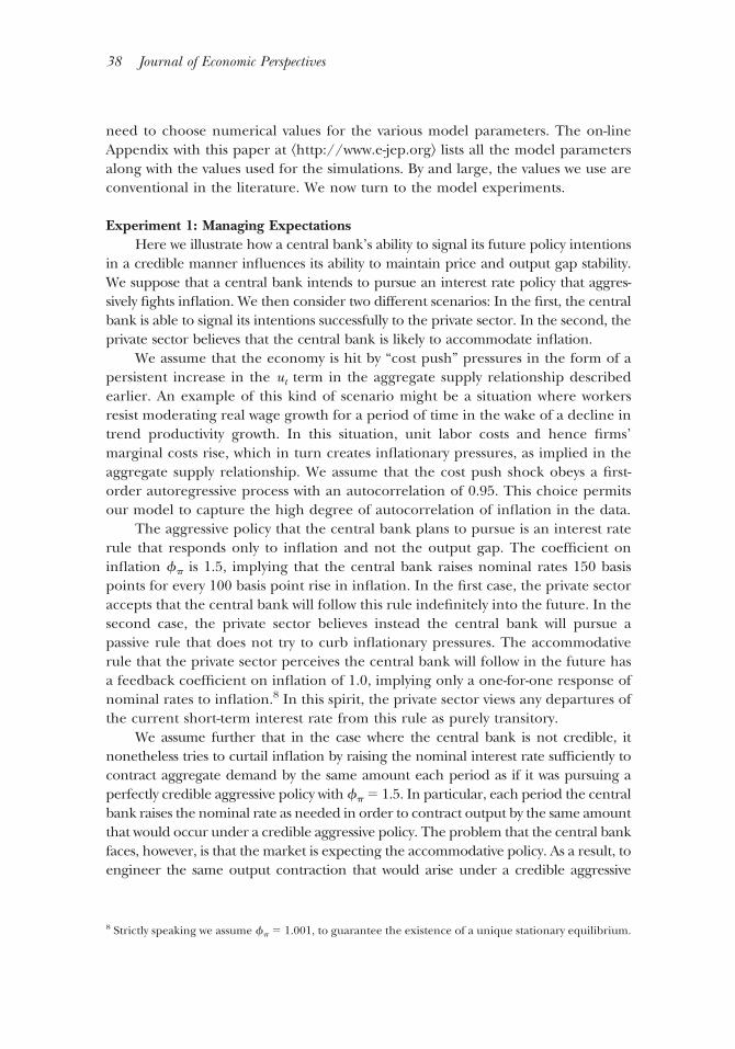
Experiment 1: Managing ExpectationsHere we illustrate how a central bank’s ability to signal its future policy intentions

in a credible manner influences its ability to maintain price and output gap stability.We suppose that a central bank intends to pursue an interest rate policy that aggres-sively fights inflation. We then consider two different scenarios: In the first, the centralbank is able to signal its intentions successfully to the private sector. In the second, theprivate sector believes that the central bank is likely to accommodate inflation.

We assume that the economy is hit by “cost push” pressures in the form of apersistent increase in the ut term in the aggregate supply relationship describedearlier. An example of this kind of scenario might be a situation where workersresist moderating real wage growth for a period of time in the wake of a decline intrend productivity growth. In this situation, unit labor costs and hence firms’marginal costs rise, which in turn creates inflationary pressures, as implied in theaggregate supply relationship. We assume that the cost push shock obeys a first-order autoregressive process with an autocorrelation of 0.95. This choice permitsour model to capture the high degree of autocorrelation of inflation in the data.

The aggressive policy that the central bank plans to pursue is an interest raterule that responds only to inflation and not the output gap. The coefficient oninflation �� is 1.5, implying that the central bank raises nominal rates 150 basispoints for every 100 basis point rise in inflation. In the first case, the private sectoraccepts that the central bank will follow this rule indefinitely into the future. In thesecond case, the private sector believes instead the central bank will pursue apassive rule that does not try to curb inflationary pressures. The accommodativerule that the private sector perceives the central bank will follow in the future hasa feedback coefficient on inflation of 1.0, implying only a one-for-one response ofnominal rates to inflation.8 In this spirit, the private sector views any departures ofthe current short-term interest rate from this rule as purely transitory.

We assume further that in the case where the central bank is not credible, itnonetheless tries to curtail inflation by raising the nominal interest rate sufficiently tocontract aggregate demand by the same amount each period as if it was pursuing aperfectly credible aggressive policy with �� 1.5. In particular, each period the centralbank raises the nominal rate as needed in order to contract output by the same amountthat would occur under a credible aggressive policy. The problem that the central bankfaces, however, is that the market is expecting the accommodative policy. As a result, toengineer the same output contraction that would arise under a credible aggressive

8 Strictly speaking we assume �� 1.001, to guarantee the existence of a unique stationary equilibrium.


policy, the central bank needs to increase sharply the current nominal interest rate.Because the private sector expects reversion to the accommodating policy in the future,to contract demand sufficiently, the central bank must compensate with an extra-largeincrease in the current short-term rate. Put differently, under the credible aggressivepolicy, the central bank exploits its ability to influence expectations over the entireyield curve. It contracts demand today not only by raising the short-term rate today, butalso by creating expectations that future short rates will be sufficiently high as well(inducing expectations of a lower output gap in the future). Without the leverage overmarket expectations, the central bank is left with the current short rate as the only wayto influence current demand.

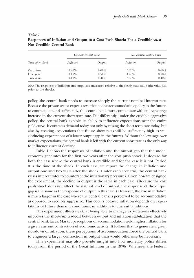
Table 1 shows the responses of inflation and the output gap that the modeleconomy generates for the first two years after the cost push shock. It does so forboth the case where the central bank is credible and for the case it is not. Period0 is the time of the shock. In each case, we report the change in inflation andoutput one and two years after the shock. Under each scenario, the central bankraises interest rates to counteract the inflationary pressures. Given how we designedthe experiment, the decline in output is the same in each case. (Because the costpush shock does not affect the natural level of output, the response of the outputgap is the same as the response of output in this case.) However, the rise in inflationis much larger in the case where the central bank is perceived to be accommodativeas opposed to credibly aggressive. This occurs because inflation depends on expec-tations of future demand conditions, in addition to current conditions.

This experiment illustrates that being able to manage expectations effectivelyimproves the short-run tradeoff between output and inflation stabilization that thecentral bank faces. Market perceptions of accommodation yield higher inflation fora given current contraction of economic activity. It follows that to generate a givenslowdown of inflation, these perceptions of accommodation force the central bankto engineer a larger contraction in output than would otherwise be necessary.

This experiment may also provide insight into how monetary policy differstoday from the period of the Great Inflation in the 1970s. Whenever the Federal

Table 1Responses of Inflation and Output to a Cost Push Shock: For a Credible vs. aNot Credible Central Bank

Time after shock

Credible central bank Not credible central bank

Inflation Output Inflation Output

Zero time 0.20% �0.60% 5.20% �0.60%One year 0.15% �0.50% 4.40% �0.50%Two years 0.10% �0.40% 3.50% �0.40%

Note: The responses of inflation and output are measured relative to the steady state value (the value justprior to the shock).


Reserve attempted to reign in inflation during this earlier period, the effort eitherhad little success or proved costly in terms of output loss. In recent times the reverseseems true. In our view, the explanation for the difference is that in the current era,the Federal Reserve has established a credible long-term commitment to maintainprice stability, which was not the case in the earlier period. This also helps explainwhy the current Federal Reserve places so much emphasis on communicating itsfuture intentions.

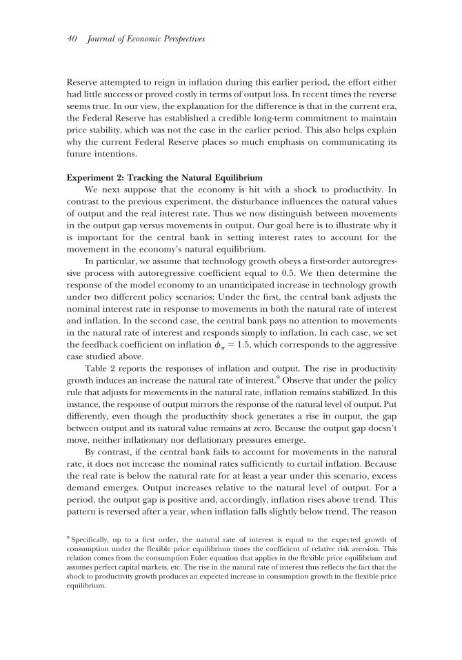
Experiment 2: Tracking the Natural EquilibriumWe next suppose that the economy is hit with a shock to productivity. In

contrast to the previous experiment, the disturbance influences the natural valuesof output and the real interest rate. Thus we now distinguish between movementsin the output gap versus movements in output. Our goal here is to illustrate why itis important for the central bank in setting interest rates to account for themovement in the economy’s natural equilibrium.

In particular, we assume that technology growth obeys a first-order autoregres-sive process with autoregressive coefficient equal to 0.5. We then determine theresponse of the model economy to an unanticipated increase in technology growthunder two different policy scenarios: Under the first, the central bank adjusts thenominal interest rate in response to movements in both the natural rate of interestand inflation. In the second case, the central bank pays no attention to movementsin the natural rate of interest and responds simply to inflation. In each case, we setthe feedback coefficient on inflation �� 1.5, which corresponds to the aggressivecase studied above.

Table 2 reports the responses of inflation and output. The rise in productivitygrowth induces an increase the natural rate of interest.9 Observe that under the policyrule that adjusts for movements in the natural rate, inflation remains stabilized. In thisinstance, the response of output mirrors the response of the natural level of output. Putdifferently, even though the productivity shock generates a rise in output, the gapbetween output and its natural value remains at zero. Because the output gap doesn’tmove, neither inflationary nor deflationary pressures emerge.

By contrast, if the central bank fails to account for movements in the naturalrate, it does not increase the nominal rates sufficiently to curtail inflation. Becausethe real rate is below the natural rate for at least a year under this scenario, excessdemand emerges. Output increases relative to the natural level of output. For aperiod, the output gap is positive and, accordingly, inflation rises above trend. Thispattern is reversed after a year, when inflation falls slightly below trend. The reason

9 Specifically, up to a first order, the natural rate of interest is equal to the expected growth ofconsumption under the flexible price equilibrium times the coefficient of relative risk aversion. Thisrelation comes from the consumption Euler equation that applies in the flexible price equilibrium andassumes perfect capital markets, etc. The rise in the natural rate of interest thus reflects the fact that theshock to productivity growth produces an expected increase in consumption growth in the flexible priceequilibrium.


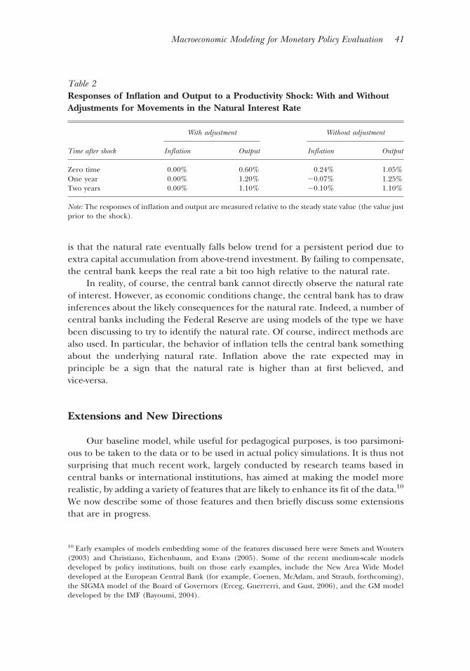
is that the natural rate eventually falls below trend for a persistent period due toextra capital accumulation from above-trend investment. By failing to compensate,the central bank keeps the real rate a bit too high relative to the natural rate.

In reality, of course, the central bank cannot directly observe the natural rateof interest. However, as economic conditions change, the central bank has to drawinferences about the likely consequences for the natural rate. Indeed, a number ofcentral banks including the Federal Reserve are using models of the type we havebeen discussing to try to identify the natural rate. Of course, indirect methods arealso used. In particular, the behavior of inflation tells the central bank somethingabout the underlying natural rate. Inflation above the rate expected may inprinciple be a sign that the natural rate is higher than at first believed, andvice-versa.

Extensions and New Directions

Our baseline model, while useful for pedagogical purposes, is too parsimoni-ous to be taken to the data or to be used in actual policy simulations. It is thus notsurprising that much recent work, largely conducted by research teams based incentral banks or international institutions, has aimed at making the model morerealistic, by adding a variety of features that are likely to enhance its fit of the data.10

We now describe some of those features and then briefly discuss some extensionsthat are in progress.

10 Early examples of models embedding some of the features discussed here were Smets and Wouters(2003) and Christiano, Eichenbaum, and Evans (2005). Some of the recent medium-scale modelsdeveloped by policy institutions, built on those early examples, include the New Area Wide Modeldeveloped at the European Central Bank (for example, Coenen, McAdam, and Straub, forthcoming),the SIGMA model of the Board of Governors (Erceg, Guerrerri, and Gust, 2006), and the GM modeldeveloped by the IMF (Bayoumi, 2004).

Table 2Responses of Inflation and Output to a Productivity Shock: With and WithoutAdjustments for Movements in the Natural Interest Rate

Time after shock

With adjustment Without adjustment

Inflation Output Inflation Output

Zero time 0.00% 0.60% 0.24% 1.05%One year 0.00% 1.20% �0.07% 1.25%Two years 0.00% 1.10% �0.10% 1.10%

Note: The responses of inflation and output are measured relative to the steady state value (the value justprior to the shock).


Taking the Model to DataThe macroeconomic variables within the baseline model appear to display

greater persistence in practice than the basic framework can capture. Forexample, the evidence suggests that a transitory exogenous shift in monetarypolicy produces a delayed hump-shaped response of the key quantity variables:output, consumption, and investment. The baseline model instead predicts aninstantaneous jump in these variables, followed by a monotonic response totrend. The reason for this is the absence of frictions that may slow down theadjustment in either consumption or investment to either current shocks, newsabout the future, or both.

A common way to address this issue is to introduce adjustment costs. In thecase of consumption, a typical approach is to assume the presence of habits inagents’ preferences, by making current utility a function of the deviation ofcurrent consumption from a benchmark usually set to be a (large) fraction oflagged consumption. Similarly, to make the model consistent with the sluggishresponse of investment to shocks, it is sometimes assumed that adjustment costsarise as a result of changes in the level of investment, as opposed to the level ofinvestment itself (relative to the capital stock) as found in the standard Tobin’sq model. (Planning lags in investment expenditure offer a plausible motivationfor this formulation.) The slow adjustment of both consumption and investmentbehavior, in turn, gives rise to hump-shaped output dynamics, consistent withthe evidence.

A further modification considered important for the empirical perfor-mance of the model is the introduction of wage rigidity. In our baseline model,we treated as exogenous the cost push shock and emphasized how variation inthis shock creates variation in inflationary pressures. The quantitative modelsendogenize movements in the cost push shock by introducing sticky nominalwages. A popular approach, due to Erceg, Henderson, and Levin (2000), is tointroduce staggered nominal wage contracting using the same kind of Calvo/Poisson adjustment process that is used to model staggered price setting. In thisenvironment, the cost push shock in the Phillips curve is no longer exogenous,but instead responds endogenously to any shock that affects the gap betweenwages and their natural equilibrium values.

New DirectionsSeveral areas of active research on these issues seem particularly interesting

to us.1. State-dependent pricing. While the models discussed above are optimization-

based, in one key aspect they are still a black box—namely the timing of price-adjustment. As we have discussed, for reasons of tractability, the models restrictattention to time-dependent pricing rules where the frequency of price adjustmentis fixed. Recently, there has been an effort to develop models based on state-dependent pricing where firms face fixed costs of price adjustment and the


adjustment frequency is determined endogenously. Examples include Dotsey, King,and Wolman (1999), Golosov and Lucas (2007), Midrigan (2006), and Gertler andLeahy (2006).

2. Labor market frictions. In existing models, all fluctuations in employmentare along the intensive margin—that is, all the variation is in hours per worker.There is no unemployment, per se. The models thus cannot account for theobserved fluctuations in unemployment and job flows. A recent and rapidlygrowing literature seeks to overcome this shortcoming by developing versions ofthe new Keynesian model that incorporate the kind of labor market frictionsfound in the search and matching literature. Examples include Walsh (2005),Trigari (2005), Blanchard and Galı (2006), and Gertler, Sala, and Trigari(2007).

3. Financial market imperfections. As we have noted earlier, the baseline modelassumes that capital markets are perfect. In many instances, this approximationmay be reasonable. However, in many situations, financial market frictions arehighly relevant considerations. In this regard, there is an on-going effort to incor-porate financial factors within the kind of quantitative macroeconomic frameworkwe have been discussing, with the aim of better understanding the appropriate roleof monetary policy in mitigating the effects of financial crises. Examples includeBernanke, Gertler, and Gilchrist (1999), Christiano, Motto, and Rostagno (2006),Monacelli (2006), and Iacoviello (2006).

Final Thoughts

The models we have described are still works in progress. Despite the recentsuccesses, we cannot be certain without further experience how resilient theseframeworks will prove as new kinds of disturbances hit the economy. Indeed, wefully expect these models to continue to evolve as we accumulate more data, andexperience more economic shocks. It may very well be the case that importantnew features are introduced and that features that seem central for per-formance today become less so in the future. At the same time, while we expectthe models to change, we think the general approach will not; quantitativemacroeconomic modeling along with its role in the policy-making process ishere to stay.

y The authors thank Jim Hines, Andrei Shleifer, Jeremy Stein, and Timothy Taylor for helpfulcomments and suggestions on an earlier draft, and Steve Nicklas for excellent researchassistance. Jordi Galı is grateful to CREA-Barcelona Economics and Ministerio de Educaciony Ciencia. Mark Gertler thanks the NSF and the Guggenheim Foundation.


References

Alvarez, Luis J. 2007. “What Do Micro PriceData Tell Us on the Validity of the New Keyne-sian Phillips Curve?” http://www.uni-kiel.de/ifw/konfer/phillips/alvarez.pdf.

Ball, Laurence, and David H. Romer. 1990.“Real Rigidities and the Nonneutrality ofMoney.” Review of Economic Studies, 57(April),183–203.

Barro, Robert, and David Gordon. 1983. “APositive Theory of Monetary Policy in a NaturalRate Model.” Journal of Political Economy, 91(4):589–610.

Bayoumi, Tam. 2004. “GEM: A New Interna-tional Macroeconomic Model.” IMF OccasionalPaper 239.

Bernanke, Ben, Mark Gertler, and Simon Gil-christ. 1999. “The Financial Accelerator in aQuantitative Business Cycle Framework.” In theHandbook of Macroeconomics, vol. 1C, ed. JohnTaylor and Michael Woodford, chapt. 21. North-Holland.

Blanchard, Olivier J., and Jordi Galı. 2006. “ANew Keynesian Model with Unemployment.”MIT, Department of Economics Working PaperNo. 06-22

Calvo, Guillermo. 1983. “Staggered Price Set-ting in a Utility Maximizing Framework.” Journalof Monetary Economics, 12(3): 383–98.

Christiano, Lawrence J., Martin Eichenbaum,and Charles L. Evans. 2005: “Nominal Rigiditiesand the Dynamic Effects of a Shock to MonetaryPolicy.” Journal of Political Economy, 113(1): 1–45.

Christiano, Lawrence J., Roberto Motto, andMassimo Rostagno. 2006. “Monetary Policyand Stock Market Boom-Bust Cycles.” http://www.ecb.int/events/pdf/conferences/cbc4/ChristianoRostagnoMotto.pdf.

Clarida, Richard, Jordi Galı, and MarkGertler. 1998. “The Financial Accelerator in aQuantitative Business Cycle Framework.” Euro-pean Economic Review, 42(6), 1033–67.

Clarida, Richard, Jordi Galı, and MarkGertler. 1999. “The Science of Monetary Policy:A New Keynesian Perspective.” Journal ofEconomic Literature, 37(4): 1661–1707.

Clarida, Richard, Jordi Galı, and MarkGertler. 2000. “Monetary Policy Rules and Mac-roeconomic Stability: Evidence and Some The-ory.” Quarterly Journal of Economics, 105(1): 147–80.

Coenen, Gunter, Peter McAdam, RolandStraub. Forthcoming. “Tax Reform and LabourMarket Performance in the Euro Area: A Simu-

lation-Based Analysis using the New Area-WideModel.” Journal of Economic Dynamics and Control.

Cogley, Timothy, and Argia M. Sbordone.2005. “A Search for a Structural Phillips Curve.”Staff Reports 203, Federal Reserve Bank of NewYork.

Dixit, Avinash, and Joseph Stiglitz. 1977. “Mo-nopolistic Competition and Optimum ProductDiversity.” American Economic Review, 67(3): 297–308.

Dotsey, Michael, Robert G. King, and Alex-ander L. Wolman. 1999. “State Dependent Pric-ing and the General Equilibrium Dynamics ofMoney and Output.” Quarterly Journal of Econom-ics, 114(2): 655–90.

Erceg, Christopher J., Luca Guerrieri, Chris-topher Gust. 2006. “SIGMA: A New Open Econ-omy Model for Policy Analysis.” InternationalJournal of Central Banking, 2(1): 1–50.

Erceg, Christopher, Dale Henderson, and An-drew Levin. 2000. “Optimal Monetary Policywith Staggered Wage and Price Contracts.” Jour-nal of Monetary Economics, 46(2): 281–313.

Fischer, Stanley. 1977. “Long Term Contracts,Rational Expectations, and the Optimal MoneySupply Rule.” Journal of Political Economy, 85(1):191–205.

Fuhrer, Jeffrey C., and George R. Moore.1995. “Inflation Persistence.” Quarterly Journal ofEconomics, 110(1): 127–159.

Galı, Jordi. Forthcoming. Monetary Policy, In-flation, and the Business Cycle. Princeton Univer-sity Press.

Galı, Jordi, and Mark Gertler. 1999. “InflationDynamics: A Structural Econometric Analysis.”Journal of Monetary Economics, 44(2): 195–222.

Galı, Jordi, Mark Gertler, and David Lopez-Salido. 2005. “Robustness of the Estimates of theHybrid New Keynesian Phillips Curve.” Journal ofMonetary Economics, 52(6): 1107–18.

Galı, Jordi, and Pau Rabanal. 2005. “Technol-ogy Shocks and Aggregate Fluctuations: HowWell Does the RBC Model Fit Postwar U.S.Data?” NBER Macroeconomics Annual 2004, 225–88.

Gertler, Mark, and John Leahy. 2006. “A Phil-lips Curve with an S-s Foundation.” Federal Re-serve Bank of Philadelphia, Working Paper 06-8.

Gertler, Mark, Luca Sala, and AntonellaTrigari. 2007. “An Estimated Monetary DSGEModel with Unemployment and Staggered NashWage Bargaining.” Unpublished paper.

Golosov, Mikhail, and Robert E. Lucas Jr.


2007. “Menu Costs and Phillips Curves.” Journalof Political Economy, 115(2): 171–99.

Goodfriend, Marvin, and Robert G. King.1997. “The New Neoclassical Synthesis and theRole of Monetary Policy.” NBER MacroeconomicsAnnual, pp. 231–82.

Hall, Robert. 2005. “Employment Fluctua-tions with Equilibrium Wage Stickiness.” Ameri-can Economic Review, 95(1): 50–64.

Iacoviello, Matteo. 2006. “House Prices, Bor-rowing Constraints and Monetary Policy in theBusiness Cycle.” American Economic Review, 95(3):739-64.

Klenow, Peter J., and Oleksiy Kryvtsov. 2005.“State-Dependent or Time-Dependent Pricing:Does it Matter for Recent U.S. Inflation?” Na-tional Bureau of Economic Research WorkingPaper 11043.

Kydland, Finn, and Edward C. Prescott. 1977.“Rules Rather Than Discretion: The Inconsis-tency of Optimal Plans.” Journal of PoliticalEconomy, 85(3): 473–91.

Lucas, Robert E. 1976. “Econometric PolicyEvaluation: A Critique.” Carnegie-Rochester Confer-ence Series on Public Policy, vol. 1, pp. 19–46.

Mankiw, N. Gregory, and David Romer. 1991.New Keynesian Economics. MIT Press; Cambridge,MA.

Midrigan, Virgiliu. 2006. “Menu Costs, Multi-Product Firms, and Aggregate Fluctuations.”http://www.ecb.int/events/pdf/conferences/intforum4/Midrigan.pdf.

Monacelli, Tommaso. 2006. “Optimal Mone-tary Policy with Collateralized Household Debtand Borrowing Constraints.” National Bureau ofEconomic Research Working Paper 12470.

Nakamura, Emi, and Jon Steinsson. 2007. “FiveFacts about Prices: A Reevaluation of Menu CostsModels.” http://www.bank-banque-canada.ca/en/conference_papers/frbc_snb/nakamura.pdf.

Prescott, Edward. 1986. “Theory Ahead ofMeasurement.” Federal Reserve Bank of Minneapo-lis Quarterly Review, Fall, pp, 9–22.

Primiceri, Giorgio, Ernst Schaumberg, andAndrea Tambalotti. 2006. “Intertemporal Distur-bances.” National Bureau of Economic ResearchWorking Paper 12243.

Rotemberg, Julio, and Michael Wood-ford.1999. “Interest Rate Rules in an EstimatedSticky Price Model.” In Monetary Policy Rules, ed.J. B. Taylor, chap. 2. University of Chicago Press.

Sargent, Thomas. 1981. “Interpreting Eco-nomic Time Series.” Journal of Political Economy,99(2): 213–48.

Sims, Christopher. 1980. “Macroeconomicsand Reality.” Econometrica, 48(1): 1–48.

Smets, Frank, and Raf Wouters. 2003. “AnEstimated Dynamic Stochastic General Equilib-rium Model of the Euro Area.” Journal of theEuropean Economic Association, 1(5):1123–75.

Smets, Frank, and Raf Wouters. 2007. “Shocksand Frictions in U.S. Business Cycles: A BayesianDSGE Approach.” American Economic Review,97(3): 586–606.

Taylor, John B. 1979. “Estimation and Controlof a Macroeconomic Model with Rational Expec-tations.” Econometrica, 47(5): 1267–86.

Taylor, John B. 1980. “Aggregate Dynamicsand Staggered Contracts.” Journal of PoliticalEconomy, 88(1): 1–23.

Taylor, John B. 1993. “Discretion versus PolicyRules in Practice.” Carnegie-Rochester Series onPublic Policy, vol. 39, pp. 195–214.

Taylor, John B. 1999. “An Historical Analysisof Monetary Policy Rules. In Monetary PolicyRules, ed. J.B. Taylor, chap. 7. University of Chi-cago Press.

Trigari, Antonella. 2005. “Equilibrium Unem-ployment, Job Flows, and Inflation Dynamics.”European Central Bank Working Paper 304.

Walsh, Carl. 2005. “Labor Market Search,Sticky Prices, and Interest Rate Rules.” Review ofEconomic Dynamics, 8(4): 829–49.

Woodford, Michael. 2001. “The Taylor Ruleand Optimal Monetary Policy.” American Eco-nomic Review, 91(2): 232–37.

Woodford, Michael. 2003. Interest and Prices:Foundations of a Theory of Monetary Policy. Prince-ton University Press: Princeton, New Jersey.

Woodford, Michael. 2006. “How Important isMoney in the Conduct of Monetary Policy?“Queen’s University, Department of Economics,Working Paper 1104.


Appendix: A Description of the Monetary Model

The operational model consists of a set of linear stochastic difference equa-tions. These equations are obtained by taking a log-linear approximation of theequilibrium conditions of the original nonlinear model, around the deterministicsteady state. That model is in turn a real business cycle model, augmented withmonopolistic competition and nominal price rigidities.

At a very general level, there are two key differences from a traditionalKeynesian framework. First, all the coefficients of the dynamical system describingthe equilibrium are explicit functions of the primitive parameters of the model, i.e.they are explicitly derived from the underlying theory. Second, expected futurevalues of some variables enter the equilibrium conditions, not only current andlagged ones. In other words, expectations matter.

As with the traditional framework, it is convenient to organize the system intothree blocks: aggregate demand, aggregate supply, and policy. In this appendix wedescribe each block, and its mathematical representation.

Aggregate DemandThe aggregate demand block consists of four equations. A central equation of

that block is given by an aggregate goods market clearing condition, i.e. a conditionequating output to the sum of the components of aggregate demand. In log-linearform we can write it as:

(AD1) yt � �c ct � �i it � dt

where y is output, c is consumption, i is investment, and dt captures the combinedeffect of other demand components (including government purchases and exter-nal demand). For simplicity we take those components as exogenous. The fourvariables are expressed in log deviations from a steady state; �c and �i represent thesteady state shares of consumption and investment in output, respectively.

The other relations characterize the behavior of each endogenous componentof spending, i.e. consumption and investment. We describe the relation for con-sumption first, and then turn to investment.

In the baseline model, both capital and insurance markets are perfect. Arepresentative household makes consumption, saving, and labor supply decisionsin this environment. Within this frictionless setting, the permanent income hypoth-esis holds perfectly. An implication is that the household strictly obeys a conven-tional Euler equation that relates the marginal cost of saving (the foregone mar-ginal utility of consumption) to the expected marginal benefit (the expected

Jordi Galı and Mark Gertler A1

product of the ex post real interest rate and the discounted marginal utility ofconsumption in the next period). Log-linearizing this equation yields a familiarpositive relation between expected consumption growth and the ex ante realinterest rate: Everything else equal, an expected rise in real rates makes the returnto saving more attractive, inducing households to reduce current consumptionrelative to expected future consumption. By rearranging this relation, we obtain thefollowing difference equation for current consumption demand:

(AD2) ct � ��rt � Et�t�1 � � Et ct�1 � �c,t ,

where rt is the nominal interest rate, �t�1 denotes the rate of price inflationbetween t and t � 1, and �c,t is an exogenous preference shock. Et is theexpectational operator conditional on information at time t. Note, in particular,that the previous equation implies that current consumption demand dependsnegatively on the real interest rate and positively on expected future consumption.

Investment is based on Tobin’s q theory. As in the conventional formulation,due to convex costs of adjustment, investment varies exactly with q, the ratio of theshadow value of the marginal unit of installed capital to the replacement value.Sufficient homogeneity is built into both the production and adjustment costtechnology to ensure that average and marginal q are the same. Accordingly, bylog-linearizing the first-order conditions for investment, we obtain a simple linearrelation between the investment–capital ratio and average q. Formally, aggregateinvestment, expressed as a ratio to the capital stock kt, is a function of (log) Tobin’sq and an exogenous disturbance �i,t:

(AD3) it � kt � � qt � �i,t .

We close the aggregate demand sector with an equation describing the evolu-tion of q. Typically, the replacement price of capital is either fixed at unity or givenexogenously. Accordingly, the endogenous variation in q comes from movement inits shadow value, which is in turn given by the discounted stream of expectedreturns to capital. By log-linearizing this relation, one obtains an expression thatrelates q to the expected path of earnings net of the expected path of short-termreal interest rates. Formally,

(AD4) qt � �1 � ��1 � �� Et�yt�1 � kt�1 � �p,t�1� � �rt � Et�t�1� � � Etqt�1,

where �p denotes the (log) price markup. Thus, we see that q depends positively onthe expected returns to investment, which in equilibrium is given by the expectedmarginal product of capital adjusted by the markup (or, equivalently, the equilib-rium rental cost) Et( yt�1 � kt�1 � �p,t�1), and negatively on its opportunity cost,given by the expected real interest rate, rt � Et�t�1.

A2 Journal of Economic Perspectives

Aggregate SupplyThere are six equations in the aggregate supply block. We begin with produc-

tion. There is a single final good, which is produced under perfect competitionusing a simple CES aggregator of intermediate goods. The only significant role ofthe final goods sector (other than transforming all intermediate goods into a singlefinal good) is to generate a downward-sloping demand for each intermediate good.

Each firm in the intermediate goods sector is a monopolistic competitorproducing a differentiated good, which it sells to the final goods sector. Productionof each intermediate good is carried out with a Cobb-Douglas technology that usescapital and labor. Formally, we have

(AS1) yt � at � �kt � �1 � ��nt .

where kt and nt respectively denote (log) capital and (log) hours, and at represents(the log of) total factor productivity. As in real business cycle models, total factorproductivity is assumed to fluctuate over time according to an exogenous process.

Each intermediate goods firm sets the price for its good given the demandcurve for its product and taking as given the wage, the rental cost of capital, and allother aggregate variables. Critically, firms do not get to readjust the price everyperiod. Instead, they set prices on a staggered basis. For simplicity, it is oftenassumed that firms use “time-dependent” pricing strategies, where they set pricesoptimally over an exogenously given horizon. Beyond the significant gain intractability, the main justification for treating the adjustment frequency as exoge-nous is that the evidence suggests that the price adjustment frequencies arereasonably stable in low-inflation economies.1 Of course, this means that themodels are mainly relevant for these kinds of environments and are certainly notappropriate for analyzing high-inflation economies. At the same time, work isunder way to relax the assumption of time-dependent pricing policies and insteadintroduce state-dependent policies where the frequency of adjustment is deter-mined endogenously.

At any point in time, accordingly, a fraction of firms adjust price, and theremaining fraction keep their prices fixed. At any time t, firms that are not settinga new price simply adjust output to meet demand, so long as the markup of priceover marginal cost remains positive. Given that marginal cost varies positively withshifts in aggregate demand, booms that move output above the natural level causeprice markups to decline for firms that do not adjust price, and vice-versa forcontractions that move output below the natural level. Thus, what ultimately makes

1 See, e.g. Klenow and Krystov (2005).

Macroeconomic Modeling for Monetary Policy Evaluation A3

cyclical departures of output from its natural level possible are countercyclicalmovements in markups stemming from price stickiness.2

Firms that are adjusting choose their respective prices optimally, given theconstraint on the frequency of price adjustment. It is typically assumed that theadjustment frequencies obey a simple model originally proposed by Calvo (1983).Each period, a firm is able to adjust its price with probability 1 � �. The realizationof this draw is independent across firms and over time. This setup capturesstaggered price setting in the simplest possible way: in each period, only thefraction 1 � � of firms are adjusting their price. The average amount of time a firmkeeps its price fixed is given by 1/(1 � �), where the parameter � is thus a measureof the degree of price rigidity. Note that � may be fixed to match the microevidenceon price adjustment frequencies.

An important virtue of this approach is that because the adjustment probabilityis independent of the firm’s history, it is not necessary to keep track of differentvintages of firms, which greatly simplifies aggregation. In this instance, to a firstapproximation, the log price level evolves as a weighted average of the log price setby those firms that adjust and the log of the average price for the firms that do notadjust—the weight on the former being simply the fraction that adjusts, 1 � �, whilethe weight on the latter is �. Formally, we have

(AS2) pt � � pt�1 � �1 � �� p*t ,

where p*t is the price set by firms adjusting their price in the current period.3

It is straightforward to show that, to a first approximation, adjusting firmschoose a price equal to a constant markup over a weighted average of current andfuture expected nominal marginal costs. Formally, this can be represented by thedifference equations

(AS3) p*t � �1 � �� wt � �yt � nt� � �� Etp*t�1 ,

where wt denotes the (log) nominal wage, and wt � ( yt � nt) is the (log) nominalmarginal cost.4 Notice that, when solved forward, the above equation (AS3) impliesthat firms choose a price to be equal to a discounted sum of current and expected

2 Because intermediate goods firms are monopolistic competitors, they have a positive desired markup;i.e. if they were free to set price each period, they would always choose a positive markup. Thus, in theflexible price equilibrium, output is below the socially efficient level. With sticky prices, booms pushoutput toward the efficient level and vice-versa for contractions. It is assumed that the boom is neverlarge enough to push output beyond the socially efficient level (i.e. the economy always operates in aregion where price exceeds marginal cost).3 Note that because the fraction that does not adjust is a random draw, the average price of thispopulation is simply last period’s economy-wide average price.4 Observe that since the production technology is Cobb-Douglas, nominal marginal costs correspond tonominal unit labor costs, i.e., nominal wages normalized by labor productivity.


future nominal marginal costs. In that discounted sum, the weight on nominalmarginal cost corresponding to any future period depends on the discountedprobability that the firm will still have its price fixed at that time. In the limiting caseof complete price flexibility (i.e. period-by-period adjustment), the firm simply setsprice as a constant markup over current nominal marginal cost.

The average price markup is given, in logs, by

(AS4) �p,t � pt � �wt � �yt � nt��.

As we noted earlier, the countercyclical markup behavior (along withprocyclical real marginal cost) emerges because nominal prices are sticky. Manyquantitative versions of these models also introduce nominal wage stickiness.This feature is not only consistent with the evidence; including it tends toimprove the overall empirical performance of the model. A common way to addwage rigidity is to assume that there exist monopolistically competitive workerswho set nominal wages on a staggered multi-period basis, in close analogy to theway firms set prices. In this context one can define a “wage markup” as thewedge between the real wage and the household’s marginal rate of substitutionbetween consumption and leisure. This relation can be expressed in log-linearform as follows:

(AS5) �w,t � �wt � pt� � mrst

� �wt � pt� � ��nt � �ct�.

In the frictionless competitive equilibrium this ratio is unity (making the log ofthis ratio zero in this case). If worker’s have some markup power, then this ratioexceeds unity. With nominal wage rigidity, the wage markup will move countercy-clically, similar to the way nominal price rigidities help generate countercyclicalprice markups. For expositional convenience here, we simply take the wage markupas exogenous, but keeping in mind that this is a stand-in for a more explicitformulation.

Finally, there is a relation for the evolution of the capital goods. Next period’scapital depends on the creation of new capital goods and what’s left of the currentcapital after depreciation. This is formalized by means of the capital accumulationequation

(AS6) kt�1 � �1 � ��kt � �it .

As we noted earlier, the creation of new capital involves convex adjustmentcost, giving rise to a variable shadow value of installed capital.

Jordi Galı and Mark Gertler A5

EquilibriumWe let variables with a tilda (˜) denote the deviation from natural values, where

the latter are defined as their equilibrium values in the absence of nominalrigidities. We denote natural variables with an “n” superscript. Thus, xt � xt � xt

n.Furthermore, we assume for simplicity that percent variations in the capital stockare small, which we approximate by setting kt � 0 for all t.

We can thus rewrite (AD2) and (AD4) in terms of gaps as:

ct � �� rt � Et�t�1 � rrtn� � Etct�1

ı t � � qt

Combined with (AD1) they imply

(1) yt � ��crr tl � �i� qt ,

where

rr tl � Et �

i�0

�

�rt�i � �t�1�i � rrt�in �.

Note that (AD3) can be rewritten as

qt � �1 � ��1 � ��Et�yt�1 � �p,t�1� � �rt � Et�t�1 � rrtn� � � Etqt�1 .

Iterating forward, qt may be expressed as

qt � Et �i�0

�

�i Etzt�1�i � �rt�1 � Et�t�1�1 � rrt�in �,

where zt � (1 � �(1 � �))( yt � �p,t). Thus holding constant current and expectedfuture interest rates, the rent to capital and hence Tobin’s q are procyclical. Conversely,holding constant the current and expected future rents to capital, qt moves inverselywith current and expected future movements in the interest rate.

We note that this equation also makes clear why most central banks arereluctant to adjust interest rates to target asset prices (see, e.g., Bernanke andGertler (2001)). First, there is no reason to believe that the central bank is betterable than the private sector to assess the fundamental determinants of asset prices,given by the right-hand side of this equation. Second, there is a circularity problem:qt is highly sensitive to the current and future path of interest rates. Thus a central


bank that mechanically adjusts interest rates to stabilize asset prices may wind upintroducing undesired volatility to either interest rates or asset prices, or both.

Furthermore, combining (AS2), (AS3), and (AS4) we obtain the aggregatesupply equation:

�t � � Et�t�1 � ��p,t ,

where

�p,t � ��

1 � �� yt � ��ct � yt � � �w,t

� ��

1 � ��

�

�c� yt �

�i

�c�� qt � �w,t .

We can thus rewrite the inflation equation in terms of the output gap as

(2) �t � � Et�t�1 � yt � ut ,

where

ut � � ��w,t ��i

�c�� qt� and � � ��

1 � ��

�

�c�.

Finally, we can represent monetary policy by means of a rule of the form:

(3) rt � �1 � ��rrtn � ��t � �yyt� � rt�1 .

Equations (1), (2), and (3) provide the canonical representation of theequilibrium dynamics of the monetary model used in a variety of applications in theliterature.

For the simulations presented in the text, we used the following parametervalues: � � 0.33; � � 0.99; � � 0.99; � � 2.0; � � 1.0; � � 0.75; �c � 0.63; �i � 0.15;� � 0.5; �� 1.5; � 0.80. In addition, we assumed that the autocorrelation of thecost push shock was 0.95.

Macroeconomic Modeling for Monetary Policy Evaluation A7

Documents

Macroeconomic Modeling for Monetary Policy Evaluation · Macroeconomic Modeling for Monetary Policy Evaluation ... term has probably become the most popular, ... These movements in