Simple Contracts with Adverse Selection and MoralHazard∗

Daniel Gottlieb and Humberto Moreira†

October, 2015

Abstract

We study a principal-agent model with moral hazard and adverse selection. Risk-neutralagents with limited liability have arbitrary private information about the distribution of out-puts and the cost of effort. We obtain conditions under which the optimal mechanism offersa small number of contracts. When output is binary, the optimal mechanism always offersthe same contract to all types. More generally, under a multiplicative separability condi-tion, the optimal mechanism offers at most two contracts. If, in addition, the principal’spayoff must be monotone (free disposal) and the distribution of outputs has the monotonelikelihood ratio property, the mechanism offers a single debt contract. Our model suggeststhat offering just one or two contracts may be optimal in environments with adverse selec-tion and moral hazard, where rich menus of contracts provide gaming opportunities to theagent. Therefore, we give an explanation for an old puzzle in contract theory: the scarcityof large menus of contracts.

∗We thank Eduardo Azevedo, Dirk Bergemann, Vinicius Carrasco, Sylvain Chassang, Gonzalo Cisternas, AlexEdmans, Eduardo Faingold, Leandro Gorno, Faruk Gul, Jason Hartline, Tibor Heumann, Bengt Holmström, Jo-hannes Hörner, Ohad Kadan, Lucas Maestri, George Mailath, David Martimort, Stephen Morris, Roger Myerson,Larry Samuelson, Yuliy Sannikov, Jean Tirole, Rakesh Vohra, John Zhu, and seminar audiences at Arizona StateUniversity, FGV, HEC Montreal, Johns Hopkins University, Princeton University, PUC-Rio, Universidad deChile, University of Pennsylvania, University of Pittsburg/Carnegie Mellon University, the Wharton School, YaleUniversity, and the BYU Computational Public Economics, 2013 LAMES, 2013 SBE, 2014 IWGTS, 2014 ESEM,2015 AEA meetings, and 2015 ESWC for comments and suggestions. Rafael Mourão provided outstanding re-search assistance. Gottlieb gratefully acknowledges financial support from the Dorinda and Mark WinkelmanDistinguished Scholar Award. Moreira acknowledges CNPq for financial support.†Gottlieb: John M. Olin School of Business, Washington University in St. Louis dgottlieb@wustl.edu. Moreira:

FGV/EPGE, humberto@fgv.br.

Contents

1 Introduction 1

2 Two Outputs 52.1 Statement of the Problem . . . . . . . . . . . . . . . . . . . . . . . . . . . . . . 52.2 Benchmarks . . . . . . . . . . . . . . . . . . . . . . . . . . . . . . . . . . . . . . 62.3 Contract Simplicity . . . . . . . . . . . . . . . . . . . . . . . . . . . . . . . . . . 8

3 Multiple Outputs 10

4 Free Disposal 13Debt Contracts . . . . . . . . . . . . . . . . . . . . . . . . . . . . . . . . . . . . . . . 15

5 Procurement and Regulation 16

6 Conclusion 19

Appendix 20Proofs . . . . . . . . . . . . . . . . . . . . . . . . . . . . . . . . . . . . . . . . . . . . 20

Theorem 1 . . . . . . . . . . . . . . . . . . . . . . . . . . . . . . . . . . . . . . . 20Theorem 2 . . . . . . . . . . . . . . . . . . . . . . . . . . . . . . . . . . . . . . . 25Proposition 1 . . . . . . . . . . . . . . . . . . . . . . . . . . . . . . . . . . . . . 34Proposition 2 . . . . . . . . . . . . . . . . . . . . . . . . . . . . . . . . . . . . . 37

Examples . . . . . . . . . . . . . . . . . . . . . . . . . . . . . . . . . . . . . . . . . . 39Multiplicative Separability . . . . . . . . . . . . . . . . . . . . . . . . . . . . . . . . . 41

References 47

Online Appendix 51

1 Introduction

Most real-world contracts are much simpler than theory predicts. Differently from standardadverse selection models, contracting parties offer a limited number of contracts, often a singleone. Unlike in standard moral hazard models, similar contracts are offered in fundamentallydifferent environments. As Hart and Holmstrom (1987) and Chiappori and Salanie (2003) arguein their surveys of the literature:

The extreme sensitivity to informational variables that comes across from thistype of modeling is at odds with reality. Real world schemes are simpler than thetheory would dictate and surprisingly uniform across a wide range of circumstances.(Hart and Holmstrom, 1987, pp. 105)

The recent literature (...) provides very strong evidence that contractual formshave large effects on behavior. As the notion that “incentives matter” is one of thecentral tenets of economists of every persuasion, this should be comforting to thecommunity. On the other hand, it raises an old puzzle: if contractual form mattersso much, why do we observe such a prevalence of fairly simple contracts? (Chiapporiand Salanie, 2003 , pp. 34)

In this paper, we propose an answer to this puzzle based on the interaction between adverseselection, moral hazard, and limited liability. Most contracting situations have both adverseselection and moral hazard. Managers, for example, take actions that affect the firm’s profitabil-ity. At the same time, they usually have better knowledge about the efficacy of each action.Moreover, virtually all contracting parties have limited liability. Entrepreneurs raising capitalfrom investors, for example, enjoy limited liability as the value of their equity cannot fall belowzero. Also, anti-slavery laws enforce limited liability in employment contracts.

We consider a principal-agent relationship with bilateral risk neutrality and limited liability.The agent selects an unobserved “effort,” which may consist of a single or multiple tasks. Theagent also has private information, in an arbitrary way, about the distribution of outputs andabout effort costs, resulting in a model where types and efforts are multidimensional (possiblyinfinite dimensional) and unordered. We show that the interaction between adverse selection,moral hazard, and limited liability imposes severe screening costs.

With binary outcomes, the optimal mechanism offers a single contract to all agents regardlessof the type space or the distribution of types. We generalize this result to settings with multipleoutputs under a multiplicative separability condition. This condition – satisfied, for example,under the spanning condition of Grossman and Hart (1983) – is equivalent to assuming thatagents rank the “power” of all contracts equally. The optimal mechanism has at most twocontracts. Additionally, if the output distribution is ordered by first-order stochastic dominance

1

and the principal’s payoff must be monotone (“free disposal”), the optimal mechanism offers asingle contract. If the output distribution also satisfies the monotone likelihood ratio property,this optimal contract consists of the principal taking a single debt contract or, equivalently,giving all agents the same call option.

More broadly, our paper identifies an important downside from offering flexibility to agentsthrough menus of contracts: gaming. This is particularly stark in the model considered here,where both the principal and the agent are risk neutral. Then, the agent always selects thecontract with the highest expected payment conditional on his effort, which is precisely thecontract with the highest cost to the principal. That is, conditional on the effort that the agentchooses, reducing the number of contracts always increases the principal’s profits (for a fixedeffort). In particular, when the principal can identify the contract with the highest and lowestpowers in a mechanism (i.e. when multiplicative separability holds), she can simultaneouslyreduce informational rents and increase efficiency by removing all intermediate contracts.

Although the framework we study has been widely applied to financial contracting, it hasmany other applications. One such application is procurement and regulation. Despite thecentral role that menus of contracts play in the theory of procurement and regulation, they arerarely observed in practice.1 Accordingly, many papers try to identify conditions for simple pro-curement contracts to be close to optimal.2 We generalize the classic model of Laffont and Tirole(1986, 1993) by allowing effort to affect the regulated firm’s costs stochastically and assumingthat the firm has limited liability. We then determine conditions for the optimal mechanism tooffer one or two contracts, and for the optimal contract to be a price cap. Since limited liabilityconstraints are a key aspect of most procurement contracts (see, e.g., Burguet et al., 2012), ourmodel provides an explanation for the absence of menus of contracts in procurement.

Our result on the optimality of simple contracts is related to the robustness intuition ofHolmstrom and Milgrom (1987). However, the notion of robustness in our static model isdifferent from the one in their seminal paper. Here, offering a single contract is robust in that itreduces the agents’ incentives to misrepresent their private information about the environment.In Holmstrom and Milgrom’s model, linear contracts are robust in the sense that they preventthe agent from readjusting effort over time.3 Moreover, as in their work, we also contribute to

1For example, Bajari and Tadelis (2001) argue that “the descriptive engineering and construction managementliterature (...) suggests that menus of contracts are not used. Instead, the vast majority of contracts are variantsof simple fixed-price (FP) and cost-plus (C+) contracts.”

2Using the Laffont-Tirole framework, Rogerson (2003) and Chu and Sappington (2007) show that a pair ofsimple contracts can achieve a large fraction of the surplus under a certain range of parametric settings – 75 or73 percent when costs follow either uniform or power distributions, respectively – for quadratic costs. Bajari andTadelis (2001) assume that there is a fixed cost of specifying each state of nature in the contract to rationalizethe simplicity of observed contracts.

3Edmans and Gabaix (2011) extend the linearity results to a model in which the realization of noise occursbefore the action. Holmstrom’s idea of robustness is different from the one used in the more recent literaturethat identifies contracts that perform well for large classes of priors. Notable contributions include Chassang(2013), who studies a class of calibrated contracts that are detail-free and approximate the performance of the

2

the applied literature by identifying assumptions under which researchers can focus on a simplerset of contracts when solving their models. For example, under the same assumptions as Innes(1990) (and, when there are more than two outputs, a multiplicative separability and an orderingassumption), there is no loss of generality in assuming that the optimal mechanism involves asingle debt contract even if there is adverse selection, making it easy to obtain comparativestatics results.

Related Literature

We consider a principal-agent relationship with bilateral risk neutrality and limited liability,as is commonly studied in corporate finance (c.f. Tirole, 2005). We build on this standardenvironment by adding adverse selection in an arbitrary way and allowing effort to be multi-dimensional. Our work is related to a literature that identifies conditions for contracts to takethe form of debt and for equilibria to have complete pooling.

In a single-task moral hazard setting where contracts must be monotone, Innes (1990) andPoblete and Spulber (2012) show that contracts take the form of debt if the distribution ofoutput satisfies the monotonicity of the likelihood ratio property. Our main focus is on the lackof menus of contracts, which, of course, can only be addressed by introducing adverse selection.Nevertheless, our Theorem 3 is reminiscent of their main result.4

In a signaling model of financial contracting, Nachman and Noe (1994) show that there iscomplete pooling if and only if firm types are strictly ordered by conditional stochastic domi-nance. When firms are ordered by conditional stochastic dominance, capitalists face a lemonsproblem: while they would like to offer better terms to healthier firms, those who are more likelyto accept the contract are precisely the least healthy firms. Our papers emphasize different forcesthat may lead to pooling. In Nachman and Noe (1994), pooling occurs when the distribution oftypes induces a market breakdown for all but the worse contract. In our model, pooling happensbecause of moral hazard and limited liability: giving flexibility to agents requires the principalto leave excessive rents. For example, when output is binary, complete pooling occurs in ourmodel for any parameters of the model (i.e. regardless of whether types are ordered).5

Similarly, Demarzo and Duffie (1999) consider a signaling model of security design and show

best linear contract in dynamic environments when players are patient, and Carroll (Forthcoming), who showsthat the best contract for a principal who faces an agent with uncertain technology and evaluates contracts interms of their worst-case performance is linear.

4See Jewitt et al. (2008) for a general analysis of moral hazard models with limited liability. Moral hazardmodels with bilateral risk neutrality, limited liability, and monotonicity include, for example, Matthews (2001),Dewatripont et al. (2003), Poblete and Spulber (2012), and Chaigneau et al. (2014). Adverse selection models inthis setting include Nachman and Noe (1994), Demarzo and Duffie (1999), DeMarzo (2005), and DeMarzo et al.(2005).

5See footnote 20 for a discussion of Nachman and Noe’s requirement that types be ordered by conditionalstochastic dominance in the context of our model.

3

that, under a uniform-worst case condition and a monotonicity constraint, equilibrium contractstake the form of debt. Using this model, several authors studied whether intermediaries pooldifferent assets in equilibrium. The conclusion depends on whether the security is designedbefore or after firms learn about the asset’s profitability (c.f., DeMarzo (2005), Biais and Mariotti(2005), and Farhi and Tirole (Forthcoming)).

In a one-dimensional adverse selection setting, Guesnerie and Laffont (1984) showed thatoptimal mechanisms are “non-responsive” when the first-best allocation is decreasing. This occursbecause optimality clashes with incentive compatibility, which requires allocations to be non-decreasing. The reason for pooling in our model is quite different from non-responsiveness. Forexample, if the agent only has private information about the distribution of output, the first bestis increasing and therefore implementable in a pure adverse selection environment. Nevertheless,with multiplicative separability, the principal at most two contracts (see footnote 13). Morerelated to our work, Ollier and Thomas (2013) substitute the traditional (interim) participationconstraint by an ex-post constraint in a one-dimensional model with binary outcomes. Theyshow that, under conditions that ensure that the first-order approach holds, there is no benefitfrom screening.

As argued previously, our application to procurement and regulation builds on Laffont andTirole (1986, 1993). In their model, there is both adverse selection and moral hazard. However,because the link between effort, types, and output is deterministic, the model can be reduced toa pure adverse selection model. For this reason, they are often referred to as models with ‘falsemoral hazard’ (c.f. Laffont and Martimort, 2002). We allow effort to affect the regulated firm’scosts stochastically so the problem cannot be reduced to a pure adverse selection model. Picard(1987), Melumad and Reichelstein (1989), and Caillaud et al. (1992) also introduce noise in therelationship between output and effort and show that, under certain conditions, the principalcan achieve the same utility as in the absence of noise. Therefore, unlike in our model, theyfind that there is no cost from moral hazard. Our model differs from theirs in two ways. First,we also allow the agent to have private information about the distribution of output, while theyassume that all private information concerns the cost of effort. Introducing private informationabout the distribution makes moral hazard costly. Second, they do not assume that agents havelimited liability. Limited liability also prevents the principal from eliminating moral hazard atno cost.

In Section 2, we present the model with two outputs and discuss the benchmark cases of pureadverse selection and pure model hazard. In Section 3, we generalize the results for multipleoutputs. In Section 4, we introduce the free disposal constraint and obtain conditions for theoptimality of debt. In Section 5, we present the application of our model to procurement andregulation. Then, Section 6 concludes. All proofs are in the appendix.

4

2 Two Outputs

2.1 Statement of the Problem

We start with a two-output model. There is a risk-neutral principal and a risk-neutral agentwith limited liability. The agent has private information about the environment, captured by atype θ ∈ Θ. From the principal’s perspective, types are distributed according to a distributionµ. We will discuss the assumptions on Θ and µ below.

The agent exerts an effort e ∈ E, which costs cθe. The space of possible efforts E is a compactmetric space. Effort can consist of a single task (E ⊂ R) or multiple tasks (E ⊂ RN). Theleast-costly effort has a non-positive cost: min

e∈Ecθe ≤ 0. This condition is satisfied in standard

frameworks where the lowest effort costs zero, as well as in more general multi-task frameworksthat allow the agent to derive private benefits from certain actions.6

The principal does not observe the effort chosen by the agent. She does, however, observethe output from the partnership x ∈ {xL, xH}, which is stochastically affected by the agent’seffort. We refer to xH as a high output or as success, to xL as a low output or failure, and to∆x := xH − xL > 0 as the incremental output. Given effort e, a high output happens withprobability pθe.

The type space Θ may be discrete or continuous, and types may be finite- or infinite-dimensional. Each type is fully characterized by the the pair of functions

(pθ· , c

θ·)specifying

the probability of success and the cost of each effort.7 For example, if effort is binary, eachtype can be described by the four-dimensional vector (pθ0, p

θ1, c

θ0, c

θ1). If effort is continuous, each

type is described by the infinite-dimensional function(pθ· , c

θ·)

: E → R2. Our model does notrequire the agent to have private information about all of these dimensions, of course. The casewhere the cost of effort e is common knowledge, for example, is accommodated by letting cθe beconstant in θ. Note that we do not impose any order on the space of types and efforts. Successprobabilities and costs may be non-monotone functions and, moreover, types and effort may becomplements, substitutes, or neither in terms of probabilities and costs.

By the revelation principle, we can focus on direct mechanisms. Let B(Θ) denote the Borelσ-field of Θ. A direct mechanism is a triple of B(Θ)-measurable functions (s, b, e) : Θ→ R2×E,consisting of fixed payments s (or salaries), bonuses b, and effort recommendations e. An agentwho reports type θ agrees to exert effort e (θ) and receives s (θ) in case of failure and s (θ)+ b (θ)

in case of success. A pair of payments s(θ) and b(θ) is called a contract.6Allowing the cost of the lowest effort to be positive makes participation random as in Rochet and Stole (2002)

and is beyond the scope of this paper.7We write pθ· to denote the function e 7−→ pθe that keeps θ constant and varies e. Similarly, p·e refers to

θ 7−→ pθe . The same notation is used for other functions.

5

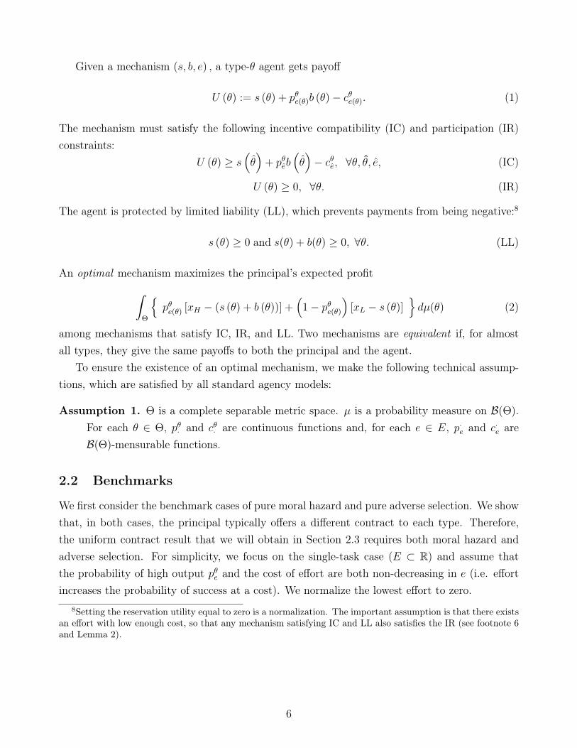
Given a mechanism (s, b, e) , a type-θ agent gets payoff

U (θ) := s (θ) + pθe(θ)b (θ)− cθe(θ). (1)

The mechanism must satisfy the following incentive compatibility (IC) and participation (IR)constraints:

U (θ) ≥ s(θ)

+ pθeb(θ)− cθe, ∀θ, θ, e, (IC)

U (θ) ≥ 0, ∀θ. (IR)

The agent is protected by limited liability (LL), which prevents payments from being negative:8

s (θ) ≥ 0 and s(θ) + b(θ) ≥ 0, ∀θ. (LL)

An optimal mechanism maximizes the principal’s expected profit

ˆΘ

{pθe(θ) [xH − (s (θ) + b (θ))] +

(1− pθe(θ)

)[xL − s (θ)]

}dµ(θ) (2)

among mechanisms that satisfy IC, IR, and LL. Two mechanisms are equivalent if, for almostall types, they give the same payoffs to both the principal and the agent.

To ensure the existence of an optimal mechanism, we make the following technical assump-tions, which are satisfied by all standard agency models:

Assumption 1. Θ is a complete separable metric space. µ is a probability measure on B(Θ).For each θ ∈ Θ, pθ· and cθ· are continuous functions and, for each e ∈ E, p·e and c·e areB(Θ)-mensurable functions.

2.2 Benchmarks

We first consider the benchmark cases of pure moral hazard and pure adverse selection. We showthat, in both cases, the principal typically offers a different contract to each type. Therefore,the uniform contract result that we will obtain in Section 2.3 requires both moral hazard andadverse selection. For simplicity, we focus on the single-task case (E ⊂ R) and assume thatthe probability of high output pθe and the cost of effort are both non-decreasing in e (i.e. effortincreases the probability of success at a cost). We normalize the lowest effort to zero.

8Setting the reservation utility equal to zero is a normalization. The important assumption is that there existsan effort with low enough cost, so that any mechanism satisfying IC and LL also satisfies the IR (see footnote 6and Lemma 2).

6

Pure Moral Hazard

Suppose the principal observes the agent’s type but does not observe effort. Without limitedliability, the principal can implement the first best by “selling the firm” to each agent – i.e.,paying a bonus equal to the incremental output b (θ) = ∆x and offering a fixed payment thatextracts the entire surplus s (θ) = cθe(θ)−pθe(θ)∆x, where e(θ) is the first-best effort. With limitedliability, the principal needs to leave rents to the agent if she wants to sell the firm. Then,it is profitable to distort the bonus downward, reducing the agent’s effort.9 Moreover, limitedliability binds, so the agent gets a zero fixed payment.

Optimal contracts with and without limited liability vary in opposite dimensions: while,without limited liability, they have the same bonus (b = ∆x) and different salaries, optimalcontracts with limited liability have the same salary (s = 0) and different bonuses.10 In bothcases, however, the principal offers different contracts to different types.11 Moreover, thesemechanisms are no longer feasible if types are unobservable. If offered contracts with the samebonus and different salaries, all types would select the one with the highest salary. Similarly, ifoffered the same salary and different bonuses, they would all pick the contract with the highestbonus. The principal can still screen unobservable types by varying both the salary and thebonus. In fact, without limited liability, this is typically optimal. Our main result shows that,with limited liability, the principal prefers not to offer a menu of contracts. Instead, the optimalmechanism offers a single contract despite the presence of many different types.12

Pure Adverse Selection

Now suppose the principal observes the agent’s effort but not his type. If effort costs arecommon knowledge (that is, θ only affects the conditional probability of success), the principalcan implement the first best by fully reimbursing the cost of each effort. The agent would be

9To see this, note that if the principal wants to recommend the lowest effort, she will pay s(θ) = b(θ) = 0and get expected payoff pθ0xH +

(1− pθ0

)xL > xL. Suppose the principal pays b(θ) ≥ ∆x and the agent exerts

effort e. The principal’s payoff is then pθe [xH − b (θ)] +(1− pθe

)xL ≤ pθe(xH −∆x) +

(1− pθe

)xL = xL .

Comparing these two inequalities, we can see that offering b(θ) ≥ ∆x is dominated by paying s = b = 0 andrecommending e = 0. Then, because agents are paid a bonus lower than the incremental output, the efforts ofall types e(θ) lie (weakly) below the first-best effort.

10For example, when there are only two efforts (say, 0 and 1) and the agent has limited liability, the principaloffers a bonus b (θ) =

cθ1pθ1−pθ0

if she recommends the high effort (e (θ) = 1). This bonus is strictly increasing in cθ1and pθ0 and strictly decreasing in pθ1.

11As we will see in Section 2.3, with both adverse selection and moral hazard, the principal offers the samecontract to all types. This optimal contract depends on the principal’s prior distribution over types. This isexpected, since the general model converges to the pure moral hazard model as the principal’s prior becomesconcentrated at a single type.

12If one showed that LL binds for all types when types are not observable, IC would imply that a single contractis offered. However, it is not obvious that the principal refrain from using different salaries and bonuses to screendifferent types. In fact, with risk aversion, LL typically does not bind for all types and the optimal mechanisminvolves menus of contracts (Gottlieb and Moreira, 2014).

7

indifferent between all efforts and would therefore accept to choose the principal’s preferredone.13 The first best can no longer be implemented when the agent has private informationabout effort costs: If the principal offered to fully reimburse the effort costs of all types, theywould all pretend to be the types with the highest costs. Conversely, if the probability of successis common knowledge (θ only affects the cost of effort), the optimal mechanism posts a paymentfor each (observed) effort and agents choose their efforts based on their privately-known costs.

As the next example illustrates, offering a menu of contracts can be optimal if the agent hasprivate information about both probabilities and costs (but effort is still observable):

Example 1. There are two efforts (0 and 1, or “low” and “high”) and two types (A and B). Theeffort costs are cA1 = 1, cB1 = 2

3, and cA0 = cB0 = 0. Given a high effort, the probability of success

for type A is pA1 = 23and for type B is pB1 = 1

3. We assume that the project fails with a high

enough probability if they exert low effort and take xH −xL to be large enough for the principalto want to implement high effort from both types.

In the appendix, we show that the optimal mechanism offers the following payments: s(A) =

0, b(A) = 32, s(B) = 2

3, and b(B) = 0. Notice that the principal uses salaries and bonuses to

screen types: type A, which has a higher probability of success, gets zero salary and a positivebonus, whereas type B, which has a lower probability of success, gets a positive salary but nobonus. Moreover, this mechanism is no longer feasible if effort is not observable, since both typeswould choose e = 0.

2.3 Contract Simplicity

We can now state the simplicity result with binary outcomes, which establishes that the principaloffers a single contract:

Theorem 1. There exists an optimal mechanism that offers a single contract (s, b) to all types,with s = 0 and b < ∆x. Moreover, any optimal mechanism is equivalent to a mechanism thatoffers the same contract to all types.

The proof is based on three lemmas. The first one shows that IC and LL imply that IR neverbinds. This follows from the fact that the agent can always guarantee himself a non-negativepayoff by picking the lowest effort and collecting the non-negative payments. The second lemmashows that any mechanism that pays a bonus greater than the incremental output to some typecannot be optimal. Any such mechanism gives the principal a payoff that is lower than if sheoffered all types a constant payment of zero.

13Note that, unlike in Guesnerie and Laffont (1984), the first-best allocation in this case is non-decreasing andis therefore feasible when the agent is not subject to moral hazard. Complete pooling in our model is due to theinteraction between adverse selection, moral hazard, and limited liability, not because of non-responsiveness.

8

The last lemma establishes that for any mechanism with bonuses lower than the incrementaloutput, if multiple contracts are being offered, the principal can improve by offering all types thecontract with the highest bonus. Since IR never binds, all agents pick this single contract onceother contracts are removed. There are two effects from this migration to the highest-poweredcontract: a reduction of rents and an increase in efficiency. Since agents are risk neutral, theypick the contract that maximizes expected payments conditional on their effort. Thus, holdingeffort fixed, reducing the set of contracts being offered decreases expected payments to the agents(rent extraction effect). Second, because agents now face a higher bonus, they choose an effortwith a higher probability of success. This raises the principal’s profit by the increased probabilityof success times the incremental output net of the bonus paid to the agent:

(pe − pe)(∆x− b),

where e is the agent’s old effort, e is the agent’s new effort, and pe ≥ pe. Since the incrementaloutput exceeds the bonus, both terms are positive. Hence, the efficiency effect is also positive.The proof then concludes by showing that an optimal mechanism exists.

Limited liability and risk neutrality play an important role in Theorem 1. Limited liabilityensures that agents do not leave the mechanism if their contract is removed. Without it, theparticipation constraint would bind for some type. Then, removing low-powered contracts wouldinduce some types to prefer not to participate. Risk neutrality implies that, holding effort fixed,the principal and the agent split a pie of a fixed size. Since the agent always picks the contractwith the highest expected payment, providing more freedom of choice to the agent can only hurtthe principal (holding effort fixed). With risk aversion, different bonuses also affect the size ofthe pie since lower bonuses insure the agent better. Then, removing all but the highest-poweredcontract improves efficiency but worsens risk sharing.

Theorem 1 greatly simplifies the analysis of the optimal mechanism by allowing us to rewritethe principal’s program as a standard optimization problem with a single instrument b ∈ [0,∆x].It is then straightforward to obtain comparative statics results. For example, using a supermod-ularity argument, we can show that the optimal bonus and the success probabilities of all typesare increasing in the incremental output ∆x. Moreover, the probability of success is distorteddownwards relative to the first best. Formally, letting eFB denote a first-best effort, we have:

eFB (θ) ∈ arg maxexL + pθe∆x− cθe and e (θ) ∈ arg max

epθeb− cθe .

Since b < ∆x, it follows by a revealed-preferences argument that pθe(θ) ≤ pθeFB(θ), with strictinequality for some type if the type space is sufficiently rich. Finally, notice that Theorem 1does not depend on the distribution of types or other parameters of the model.

It is straightforward to generalize the analysis above to the case of multiple outputs when

9

contracts are restricted to two-part tariffs, where the fixed part corresponds to a wage that is paidindependent of the output and the variable part corresponds to equity payments that are linear inthe firm’s output. The restriction to two-part tariffs can be motivated by arbitrage opportunitieswhen the principal deals with multiple agents who can costlessly redistribute outputs betweenthemselves. In the next section, we study optimal contracts without this restriction.

3 Multiple Outputs

We now generalize the model to allow for multiple outputs. Let X := {x1, ..., xN} be the setof possible (real-valued) outputs with x1 < ... < xN . As before, the agent’s private informationis described by a type θ ∈ Θ. Types are distributed according to a probability measure µ onB(Θ). Notice that our formulation allows types to be finite- or infinite-dimensional, and theirdistribution may be discrete or continuous.

The agent chooses an unobservable effort e from the compact metric space E. A type-θ agentwho exerts effort e produces output xi with probability pθe (xi) := Pr(x = xi|θ, e). Let cθe denotetype θ’s cost of of effort e. As before, we assume that the least-costly effort has a non-positivecost: mine c

θe ≤ 0 for all θ.

A contract is a function that specifies a transfer to the agent conditional on each possibleoutput. A mechanism specifies a contract and an effort recommendation for each type. That is,a mechanism is a pair of measurable functions w : Θ×X → R and e : Θ→ E, so that a type-θagent is recommended effort e (θ) and gets paid wθ (x) in case of output x.

Given a mechanism (w, e), a type-θ agent gets expected payoff

U (θ) :=N∑i=1

wθ (xi) pθe(θ) (xi)− cθe(θ).

As in the two-output case, the mechanism has to satisfy the following IC, IR, and LL constraints:

U (θ) ≥N∑i=1

wθ (xi) pθe (xi)− cθe, ∀θ, θ, e, (IC)

U (θ) ≥ 0, ∀θ, (IR)

wθ (xi) ≥ 0, ∀θ, i. (LL)

An optimal mechanism maximizes the principal’s expected profit

ˆΘ

N∑i=1

[xi − wθ(xi)

]pθe(θ)(xi)dµ(θ) (3)

10

among mechanisms that satisfy IC, IR, and LL.The main question we address in this section is whether there exists an optimal mechanism

that offers at most two contracts to all types – that is, whether there exist wL and wH such that,for each θ, either wθ(x) = wL(x) for all x or wθ(x) = wH(x) for all x. The example below showsthat, without additional restrictions, the answer is no.

Example 2. There are N ≥ 3 types and N + 1 states: Θ = {1, ..., N} and X = {x0, x1, ..., xN}.There are two efforts, E = {0, 1}, and all types have the same effort costs: cθ0 = 0 and cθ1 = 1

for all θ. The conditional probability of each output is

pθ1(x) =

{12

if x = xθ1

2Nif x 6= xθ

and pθ0(x) =

{1 if x = x0

0 if x 6= x0

.

That is, output always equals x0 if the agent exerts low effort. Any output is possible with higheffort, although each type’s “own output” (xθ) is the most likely outcome. Suppose that x0 islow enough, so that it is optimal for the principal to implement high effort from all types.

As we show in the appendix, the optimal mechanism offers the following contracts:

wθ (x) =

{2 if x = xθ

0 if x 6= xθ.

Each type’s contract pays 2 if the output matches the agent’s own type and zero otherwise.Therefore, the optimal mechanism consists of S different contracts, one for each type.

The example illustrates the main problem in generalizing Theorem 1 to multiple outputs.With two outputs, the only way to incentivize effort is to pay a higher bonus. The power ofany contract is determined by its bonus.14 With multiple outputs, there is one bonus associatedwith each incremental output, so contract power has, in general, only a partial order. A contractthat convinces one type to exert effort may be ineffective in incentivizing another type. In theexample, the cheapest way to incentivize type θ to exert effort was to pay a bonus in case ofoutput xθ.

To rule out cases such as the one in Example 2, where types disagree over the effectivenessof incentives, we need to ensure that types order the power of different contracts in the sameway. Formally, we need the following property to hold. Let w and w be two contracts satisfyingLL. If there exist e0, e0 ∈ E and θ0 ∈ Θ for which

N∑i=1

w(xi)[pθ0e0(xi)− p

θ0e0

(xi)]

=N∑i=1

w(xi)[pθ0e0(xi)− p

θ0e0

(xi)],

14Similarly, when the contract space is restricted to two-part tariffs, we can unequivocally rank the power oftwo contracts by their slopes.

11

then, for all θ ∈ Θ and all e, e ∈ E,

N∑i=1

w(xi)[pθe(xi)− pθe(xi)

]=

N∑i=1

w(xi)[pθe(xi)− pθe(xi)

].

This condition states that if one type has the same incentives to exert two efforts under contractsw and w, so do all other types for any two efforts. In other words, all types agree on the incentivesprovided by each contract. Of course, they may still pick different efforts depending on theirdistributions and effort costs. However, this condition rules out cases such as Example 4, wherethe principal increases effort from each type by offering a contract that pays a higher bonus ina different state.

Although intuitive, this is a somewhat convoluted assumption. As we show in Appendix C,however, this assumption is equivalent to the following multiplicative separability (MS) condi-tion:15

Definition 1. A cumulative distribution F θe satisfies multiplicative separability (MS) if there

exist functions H : X → R and I : E ×Θ→ R such that

F θe (x) + I(e, θ)H(x) = F θ

e (x) + I(e, θ)H (x) ∀e, e, θ, x. (4)

Multiplicative separability always holds when there are only two outputs. It also holdsunder the Linearity of the Distribution Function Condition (Grossman and Hart 1983; Hartand Holmstrom 1987), which is obtained by taking E = [0, 1], I (e, θ) ∈ [0, 1], and H(x) =

F0(x)− F1(x) for some distributions F0 and F1:

F θe (x) = I(e, θ)F1 (x) + [1− I(e, θ)]F0 (x) . (5)

This condition is commonly used in pure moral hazard models, along with the convexity of costs,to justify the first-order approach. Importantly, however, none of our results assume the validityof the first-order approach.16

The following technical conditions, which generalize Assumption 1, guarantee the existenceof an optimal mechanism:17

Assumption 2. i) cθe and pθe(xi) are continuous functions of (e, θ); and15In Appendix C, we also give a graphical characterization of distributions satisfying MS.16There is no relationship between MS and Holmstrom’s (1979) sufficient statistic result. For example, MS

always holds with binary outputs. However, as long as the likelihood ratiopθeH

(x)

pθeL(x)

is not constant in θ for some

efforts eL and eH , x will not be not a sufficient statistic for e given (x, θ). Moreover, because types also affectthe cost of effort, the optimal pure-moral-hazard contract is also a function of θ even if types do not affect thelikelihood ratio (see footnote 10).

17Assumption 2. i requires joint continuity of c and p on (e, θ), which is needed in the proof of Theorem 2. Forour other results, only continuity with respect to e and measurability with respect to θ are required.

12

ii) pθe (xi) ≥ p for some p > 0.

The next theorem shows that whenever MS holds, the optimal mechanism offers at most twocontracts.18 Types who are offered the same contract may still choose different efforts, however,depending on their distributions and effort costs.

Theorem 2. Suppose MS holds. There exists an optimal mechanism that offers at most two con-tracts to all types. Moreover, for any optimal mechanism, there exists an equivalent mechanismthat offers at most two contracts to all types.

Recall that with two efforts, substituting all contracts by the one with the highest bonus hadtwo effects. First, holding effort fixed, it reduced the expected payment to all types. Second, itincreased the probability of success, which raised the principal’s profit because the bonus waslower than the incremental output. The first of these effects remains unchanged with multipleoutputs: holding effort fixed, the principal and the agent split a pie of fixed size (since theyare both risk neutral). Therefore, for any fixed effort, removing a contract from the mechanismcannot hurt the principal.

The main difficulty with multiple outputs is with the second effect. High-powered contractsmay be unprofitable for two reasons. First, a high-powered contract may incentivize an inefficienteffort. Second, because some bonuses may exceed the incremental output (i.e., xi+1 − xi <

wi+1−wi for some i), improving the distribution of outputs may decrease the principal’s profits.Addressing these issues requires the principal to offer two contracts: a high-powered contractto types whose effort she wants to encourage and a low-powered contract to those whose effortshe wants to discourage. We show that if the principal removes from a mechanism all contractsexcept for the ones with the highest and the lowest incentives, types whose effort is profitable pickthe high-powered contract and types whose effort is unprofitable pick the low-powered contract.Therefore, the second effect is also positive.

4 Free Disposal

We now introduce the following free disposal (FD) constraint in the multiple-output environmentfrom Section 3:

y − wθ (y) ≥ x− wθ (x) (FD)

for all θ ∈ Θ and all x, y ∈ X with y ≥ x. Because FD requires the principal’s profit to be non-decreasing, we follow Matthews (2001) and call it a monotonicity constraint.19 As Innes (1990)

18MS can be slightly weakened since it does not need to hold for all efforts, only the ones that principal maywant to implement. For example, Theorem 2 remains unchanged if (4) fails at points where F θ· (x) and cθ· arelocally concave (since such efforts are not implementable).

19FD still allows the agent’s payment wθ(x) to be non-monotonic. All the results from this section continueto hold if we also impose monotonicity on the agent’s side (as well as limited liability on the principal). In

13

argues, FD can be seen as an additional incentive constraint if the principal can costlessly reduceoutput or if the agent can borrow from outside lenders to inflate output. An optimal monotonemechanism maximizes the principal’s expected profit (3) among mechanisms that satisfy IC, IR,LL, and FD.

Let F θ :={F θe : e ∈ E

}be a family of distributions satisfying MS. We say that F θ is ordered

by first-order stochastic dominance (FOSD) if the distributions can be written as in equation (4)and F θ

e (x) first-order stochastically dominates F θe (x) if and only if I(e, θ) ≤ I(e, θ).20 That is,

I(e, θ) orders the output distributions in terms of FOSD. Economically, in a family ordered byFOSD, the order of expected payments under different efforts is the same for any non-decreasingpayments. This is a standard assumption in single-task models, where we typically assume thateffort orders the output distribution in terms of FOSD. This is a less compelling assumption inmulti-task models. It fails, for example, if the agent allocates effort to a safe and a risky task,and effort allocated to the risky task increases both the mean and the variance of output.

Following the same steps as Theorem 2, we can show that the optimal monotone mechanismoffers at most two contracts. We now show that if distributions are ordered by FOSD, theoptimal monotone mechanism offers a single contract:21

Lemma 1. Suppose MS holds and F θ is ordered by FOSD for all θ. Then, there exists anoptimal monotone mechanism that offers the same contract to all types. Moreover, any optimalmonotone mechanism is equivalent to a mechanism that offers the same contract to all types.

Recall that, in general, the principal does not want to encourage effort from all types. Butwhen distributions are ordered by FOSD, the ranking of payments is the same for any non-decreasing payments. Since FD requires the principal’s payment to be non-decreasing, offeringthe contract with the highest incentives is always profitable. Therefore, a single contract sufficesto implement the optimal mechanism.

While Lemma 1 shows that MS and FOSD are sufficient conditions for the optimal mechanismto involve a single contract, they are not necessary. Choosing outputs appropriately in Example2 (so that FD does not bind) shows that the optimal mechanism may involve as many contractsas types if the distribution is ordered by FOSD but does not satisfy MS (see the supplementaryappendix). However, as we show in Appendix D, offering a single contract is optimal under aslightly more general condition than MS.

particular, when debt contracts are optimal (Theorem 3), adding either of these constraints would not modifythe optimal contract.

20In the pure adverse selection model of Nachman and Noe (1994), project types are assumed to be ranked interms of first-order stochastic dominance, which is fundamentally different than assuming that, for each type θ,effort orders outputs in terms of FOSD. We do not require types to be ordered in any way.

21Lemma 1 and Theorem 3 only require that, for each e ∈ E, p·e and c·e are measurable functions in Assumption2 (ii).

14

Debt Contracts

Next, we consider the optimality of debt contracts. The principal gets a debt contract if hispayments x−w (x) equal min {x, x} for some face value x, or, equivalently, if the agent is givena call option w (x) = max {x− x, 0}. Incentive-compatible mechanisms cannot offer more thanone debt contract, since agents would always pick the one with the lowest face value. Therefore,for a mechanism to offer debt contracts only, it needs to offer the same contract to all types.Accordingly, we assume that MS holds and F θ is ordered by FOSD for all θ, so the principaloffers a single contract.

The existing literature established that, in the single-task version of the model (E ⊂ R)with pure moral hazard, the monotone likelihood ratio property (MLRP) is sufficient for theoptimality of debt. In this one-dimensional effort model, a probability mass function pθe satisfiesMLRP if, for any eL, eH with eL < eH , the ratio

pθeL(x)

pθeH(x)

is decreasing in x. Intuitively, MLRPmeans that the “evidence” in favor of higher efforts increases with output. MLRP, which isimplied by FOSD, plays an important role on the monotonicity of contracts (Holmstrom (1979);Grossman and Hart (1983)). Accordingly, we work with the following notion of MLRP:

Definition 2. A distribution satisfying MS has the monotone likelihood ratio property if itcan be written as in equation (4) and

pθeH(x)

pθeL(x)

is increasing in x for any eL, eH , and θ withI(eH , θ) > I(eL, θ).

Our next result establishes that when, in addition to the conditions from Lemma 1(b), thedistributions satisfy MLRP, not only is it optimal to offer only one contract, but this contracttakes the form of debt:

Theorem 3. Suppose MS holds and the distributions satisfy MLRP. There exists an optimalmonotone mechanism that gives the principal a single debt contract. Moreover, any optimalmonotone mechanism is equivalent to a mechanism that gives the principal a single debt contract.

The intuition for the optimality of debt is reminiscent of Innes (1990). With MLRP, higheroutputs are more “indicative” of higher effort. Therefore, transferring payments from lower tohigher outputs relaxes the IC constraints.

In the canonical pure moral hazard model, there is a single IC, preventing the agent fromchoosing a lower effort. Here, because of adverse selection, there is one IC for each type, whichprevents each type from picking a different effort. However, because of multiplicative separabilityand ordering by FOSD, the ICs of all types are aligned, in the sense that if a perturbation raisesone type’s incentives to exert effort, it must also raise the incentives of all types. This observationallows us to summarize all the constraints of the program into a single one, as in the pure moralhazard model.

15

5 Procurement and Regulation

In this section, we adapt our main framework to a setting of procurement and regulation thatbuilds on the classic framework of Laffont and Tirole (1986, 1993). Their model can be reducedto a pure adverse selection model because effort affects the regulated firm’s cost deterministically.Our model incorporates moral hazard in their model by allowing effort to affect the firm’s coststochastically.

A regulated firm produces an indivisible good that generates a consumer surplus of S > 0 ata random monetary cost C ∈ {C1, ..., CN} with C1 < ... < CN . The firm’s manager chooses acost-reducing effort e ∈ E, which is not observed by the regulator. Let pθe denote the probabilitythat the firm’s cost equals C conditional on type θ and effort e.

The firm’s manager has cost of effort cθe, with mine cθe ≤ 0. As argued previously, this

is satisfied if the lowest effort costs zero or if the manager gets private benefits out of someactivities. The firm’s manager has private information about both his ability to cut costs (i.e., theconditional distribution of costs pθe) and the cost of effort cθe. The regulator observes the monetarycost C incurred by the firm but not the manager’s effort e. As an accounting convention, assumethat the regulator reimburses the firm’s monetary costs in addition to paying the firm an amountconditional on the observed cost C.

A contract is a function that specifies a transfer to the firm conditional on each possible costC. A mechanism is a pair of measurable functions w : {C1, ..., CN} × Θ → R and e : Θ → Rspecifying, for each reported type, a recommended effort and a transfer for each cost realization.Given a mechanism (w, e) , a type-θ manager gets payoff

U(θ) :=N∑i=1

wθ (Ci) pθe(θ) (Ci)− cθe(θ). (6)

As usual, the mechanism must satisfy the IC and IR constraints

U (θ) ≥N∑i=1

wθ (Ci) pθe (Ci)− cθe, ∀θ, θ, e, (IC)

U (θ) ≥ 0, ∀θ. (IR)

The manager is protected by limited liability, so that payments are non-negative:

wθ(C) ≥ 0, ∀C. (LL)

We impose the technical conditions from Assumption 2 (with C instead of x).Since, by the accounting convention described above, the regulator fully reimburses the firm’s

16

cost realization, the regulator’s expected payment to type θ equals

N∑i=1

[Ci + wθ (Ci)

]pθe(θ) (Ci) .

Because the government uses distortionary taxation to raise public funds, the regulator faces ashadow cost of public funds λ > 0. The net surplus of consumers/taxpayers is

S − (1 + λ)N∑i=1

[Ci + wθ (Ci)

]pθe(θ) (Ci) . (7)

A utilitarian regulator maximizes the sum of the expected utility of the firm’s manager (6) andthe consumers’ net surplus (7):

S − (1 + λ)N∑i=1

Cipθe(θ) (Ci)− cθe(θ) − λ

N∑i=1

wθ (Ci) pθe(θ) (Ci) .

As the last term of this expression shows, because taxation is distortionary (λ > 0), leaving rentsthe the regulated firm is costly. Moreover, because each dollar reimbursed to the firm has anadditional cost of λ due to distortionary taxation, cutting the firm’s cost increases social surplusby 1 + λ. The first-best effort minimizes (1 + λ)

∑Ni=1Cip

θe (Ci) + cθe.22

The main difference between this model and the principal-agent model considered previouslyis that, while the principal only cares about her own payoff, a utilitarian regulator also caresabout the manager’s payoffs. Therefore, the regulator also internalizes the manager’s effort costso their preferences are not perfectly misaligned. However, to avoid distortionary taxation, theregulator would still like to leave as little rents as possible to the firm’s manager.

We can now state the simplicity result for the case of binary outcomes:

Proposition 1. Suppose there are two possible monetary costs (N = 2). There exists an optimalmechanism that offers the same contract to all types. Moreover, for any optimal mechanism,there exists an equivalent mechanism that offers the same contract to all types.

The proof of Proposition 1 is similar to the one from Theorem 1, with one key difference.Because the regulator internalizes the cost of effort, to show that the bonus must be lower than

22If types were observable and the firm did not have limited liability, the regulator would implement the firstbest by making the firm the residual claimant of the social gain from cutting costs and extracting the entiresurplus:

wθ(Ci) = (1 + λ)

[N∑i=1

CipθeFB(θ)(Ci)− Ci

],

where eFB(θ) is the first-best effort. This violates LL because w is non-degenerate and has mean zero.

17

the one that implements the first best, we substitute contracts by the one that “sells the firm”to the manager (rather than the contract that always pays zero, as in Theorem 1).

Next, we consider the case of multiple outputs N > 2. As in Section 4, contracts must satisfythe following free disposal constraint:

wθ (Cj)− wθ (Ci) ≤ Ci − Cj (FD)

for all j and i with i > j. FD requires the firm’s compensation for cutting costs not to exceedthe amount cut. It must be satisfied, for example, if the firm’s manager can secretly borrowfrom an outside party to inflate firm earnings. An optimal monotone mechanism maximizes theprincipal’s expected profit (3) among mechanisms that satisfy IC, IR, LL, and FD.

As in Section 4, we assume that the cost distributions satisfy MS and are ordered by FOSD.Notice that, differently from output in the principal-agent model, a higher cost decreases theprincipal’s payoff. We therefore say that the cost distribution satisfies MLRP if, for any eL, eH ,and θ with I(eH , θ) > I(eL, θ),

pθeH(C)

pθeL(C)

is decreasing in C. That is, higher costs are indicative of“less effort” (more precisely, they are indicative of a lower I(e, θ)).

Adapting Lemma 1 and Theorem 3, we obtain the following results:

Proposition 2. Suppose MS holds and the family of distributions is ordered by FOSD.a) There exists an optimal monotone mechanism that offers the same contract to all types.Moreover, for any optimal monotone mechanism, there exists an equivalent mechanism thatoffers the same contract to all types.b) Suppose, in addition, that the distributions satisfy MLRP. Then, there exists an optimalmonotone mechanism that offers to all types the contract w (C) = max

{C − C; 0

}, for some

C. Moreover, for any optimal monotone mechanism, there exists an equivalent mechanism thatoffers to all types the contract w (C) = max

{C − C; 0

}, for some C.

The optimal contract in part (b) specifies a “reasonable cost” C and reimburses the regulatedfirm for any cost cuts beyond C. Since, by our accounting convention, the regulator pays thefirm’s cost directly, the firm’s revenues under this contract equal:

w(C) + C = max{C, C

}.

This reimbursement rule consists of a standard price cap except that, because of limited liabil-ity, the regulator must bailout firms with cost realizations above the cap. Price caps are themost common form of incentive regulation. They are used, for example, by the U.S. FederalCommunications Commission (FCC) to regulate the telephone industry. Price caps are oftenused in procurement as well. For example, prospective reimbursement systems commonly usedin health care specify an amount C based on what a service should cost, and let providers keep

18

cost savings C − C to themselves. They are used, for example, by Medicare.

6 Conclusion

The observation that many contracts are simple and relatively uniform across different sectorsis an old puzzle in contract theory. While standard adverse selection models predict that agentswill be offered large menus of contracts, contracting parties typically offer a limited numberof contracts, often a single one. While standard moral hazard models predict that contractsshould be fine tuned to the likelihood ratio of output, similar contracts are offered in differentenvironments.

We argue that these two features endogenously emerge in a general model of moral hazardand adverse selection if contracts must satisfy limited liability. With binary outcomes, theprincipal always offers a single contract regardless of any parameters of the model. The jointpresence of moral hazard and adverse selection is key for this result. When either types oreffort are observed, the principal typically prefers to offer different contracts to different types.With multiple outputs, it is optimal to offer two contracts if the distribution of output satisfiesa separability condition. Moreover, if the marginal distribution satisfies MLRP, this optimalmonotone contract is a debt contract for the principal.

Our paper shows that gaming may be an important downside from giving flexibility to agentsby offering menus of contracts. This is particularly stark with bilateral risk neutrality where,holding effort fixed, the agent always selects the most expensive contract to the principal. Then,reducing the number of contracts offered to the agent always increases the principal’s profits (fora fixed effort). If, in addition, we can identify a most efficient contract from the menu (such aswhen output is binary or when the distribution is multiplicatively separable and ordered), theprincipal can always improve by eliminating other contracts.

The simplicity results rely on the presence of limited liability and bilateral risk neutrality.Limited liability ensures that increasing the power of a contract will not force the agent toabandon the mechanism. Bilateral risk neutrality means that, holding effort fixed, principaland agent are perfectly misaligned so that the principal always benefits by reducing the agent’sflexibility. With risk aversion, their misalignment is no longer perfect because there are potentialgains from risk-sharing. While risk neutrality is a reasonable assumption in many settings (suchas the optimal compensation of wealthy managers, procurement contracts, or the regulation oflarge companies), there are many other settings where they are not (for example, insurancecontracts or sharecropping). In these cases, our results no longer hold. In our companion paper(Gottlieb and Moreira 2014), we study optimal mechanisms in the binary-outcome model whenagents are risk averse and when there are no limited liability constraints. While we obtain somesimplicity results, optimal mechanisms are considerably more complex than they are here.

19

Appendix

A. Proofs

Proof of Theorem 1

We first verify that participation is implied by incentive compatibility and limited liability:

Lemma 2. Let (s, b, e) be a mechanism that satisfies IC and LL. Then, it satisfies IR.

Proof. The IC preventing θ from deviating to e states that U (θ) ≥ s (θ) + pθeb (θ) − cθe. Then,because s(θ) and b(θ)+s(θ) are non-negative (LL) and min

e∈Ecθe ≤ 0, it follows that U (θ) ≥ 0.

The proof of the theorem will use the following result, which states that the bonus does notexceed the incremental output:

Lemma 3. Consider a mechanism (s, b, e) in which b (θ) > ∆x for some θ. Then, there existsanother mechanism that gives the principal a greater payoff than (s, b, e).

Proof. In any optimal mechanism, the limited liability constraint must bind for some type.Otherwise, reducing the fixed payment to all types by a uniform amount maintains feasibilityand increases the principal’s payoff.

Let (s, b, e) be an optimal mechanism with b(θ) > ∆x for some type θ. If all types havebonuses greater than the incremental output (b(θ) > ∆x), the principal’s payoff is strictly lowerthan the one she obtains by offering s = b = 0 to all types, which contradicts optimality.

Suppose there exists a type θ who picks a contract with b(θ) ≤ ∆x. Because LL must bindfor some type θH , this type must pick a contract with bH := b(θH) > ∆x (otherwise, the contract(0, bH) with bH ≤ ∆x would be first-order stochastically dominated by the contract that payss(θ) ≥ 0 and b(θ) > ∆x, which is offered by assumption). Therefore, the mechanism includes atleast one contract (sL, bL) with bL ≤ ∆x and contract (0, bH) with bH > ∆x. We claim that thismechanism gives the principal a lower profit on all types than offering s = b = 0 to all types.

For each θ, let e(θ) ∈ arg mine∈E

cθe. The principal’s profit from a type θ who chooses contract

(0, bH) and exerts effort eH ∈ E is

xL + pθeH (∆x− bH).

Replacing this contract by s = b = 0 changes the principal’s payoff to xL + pθe(θ)

∆x, increasingprofits by

pθe(θ)

∆x+ pθeH (bH −∆x) > 0.

20

The principal’s profit from a type θ who chooses (sL, bL) and exerts effort eL ∈ E is

xL − sL + pθeL(∆x− bL).

By the incentive compatibility constraint of a type who picks (sL, bL) and the fact that bH > ∆x,

pθeL∆x < pθeLbH ≤ sL + pθeLbL.

Adding xL to all terms in this inequality and rearranging, gives

xL + pθeL∆x−(sL + pθeLbL

)< xL.

Add pθe(θ)∆x ≥ 0 to the expression on the right to obtain:

xL + pθeL∆x−(sL + pθeLbL

)< xL + pθe(θ)∆x.

The term on the right is the principal’s profit from the constant-payment contract (s = b = 0)whereas the term on the left is the profit from the original contract. Hence, this replacementalso raises profits from any type who chooses a contract with b(θ) ≤ ∆x.

The next lemma, which is the main step for proving Theorem 1, shows that any feasiblemechanism is weakly dominated by a mechanism that offers a single contract to all types:

Lemma 4. Let (s, b, e) be a mechanism satisfying IC, IR, and LL. There exists a mechanismthat offers a single contract (0, b∗) to all types and gives the principal a (weakly) greater payoffthan (s, b, e).

Proof. Let (s, b, e) be a mechanism that satisfies IC, IR, and LL. By Lemma 3, for any mechanismthat offers a bonus greater than ∆x for some type, there exists another mechanism offeringbonuses lower than ∆x to all types that gives the principal a higher payoff. Thus, there is noloss of generality in assuming that b(θ) ≤ ∆x for all θ ∈ Θ. Fix a type θ ∈ Θ.

Let b∗ ≡ sup{b(θ) : θ ∈ Θ

}and s∗ ≡ inf

{s(θ) : θ ∈ Θ

}denote the “highest” bonus and

the “lowest” fixed payment in the mechanism. If s∗ > 0, reducing all fixed payments uniformlyby s∗ would keep all the constraints satisfied and increase the principal’s payoff. Therefore, wecan assume that s∗ = 0. Moreover, either there exists θ such that s(θ) = 0, b(θ) = b∗ (i.e., (0, b∗)

is offered in the mechanism), or (0, b∗) is a limit point of{(s(θ), b(θ)

); θ ∈ Θ

}.

Consider the alternative mechanism that offers the contract (0, b∗) to all types and let

e∗ (θ) ∈ arg maxe∈E

pθeb∗ − cθe,

21

which exists because the objective function is continuous and E is compact. The principal’spayoff from type θ in the original mechanism is

xL − s(θ) + pθe(θ) [∆x− b(θ)] . (8)

Her payoff in the alternative mechanism is

xL + pθe∗(θ)(∆x− b∗). (9)

Since the contract (0, b∗) either belongs to, or is a limit point of the original mechanism, noagent can be better off by switching to (0, b∗) while holding the recommended effort fixed:

s(θ) + pθe(θ)b(θ)− cθe(θ) ≥ pθe(θ)b∗ − cθe(θ).

(This inequality follows from type θ’s incentive constraint while holding e(θ) fixed). Adding cθe(θ)to both sides, it follows that the expected payment in the alternative mechanism cannot exceedthe one from the original mechanism if effort is held constant:

s(θ) + pθe(θ)b(θ) ≥ pθe(θ)b∗. (10)

That is, if the agent chooses not to change effort (e∗(θ) = e(θ)), the principal obtains a higherpayoff in the alternative mechanism (9) than in the original one (8). Allowing effort to change,the principal’s payoff in the alternative mechanism minus the payoff in the original mechanismbecomes

pθe∗(θ)(∆x− b∗)− pθe(θ) [∆x− b(θ)] + s(θ) =(pθe∗(θ) − pθe(θ)

)(∆x− b∗) + s(θ) + pθe(θ)b (θ)− pθe(θ)b∗

≥(pθe∗(θ) − pθe(θ)

)(∆x− b∗),

(11)where the inequality follows from (10).

By assumption, ∆x ≥ b∗. We claim that pθe∗(θ) ≥ pθe(θ). To wit, by the incentive constraint oftype θ in the original mechanism,

s(θ) + pθe(θ)b(θ)− cθe(θ) ≥ s(θ) + pθe∗(θ)b(θ)− cθe∗(θ),

and, by the definition of e∗(θ),

pθe∗(θ)b∗ − cθe∗(θ) ≥ pθe(θ)b

∗ − cθe(θ).

22

Rearranging both inequalities, we can write them as:

(pθe∗(θ) − pθe(θ)

)b∗ ≥ cθe∗(θ) − cθe(θ) ≥

(pθe∗(θ) − pθe(θ)

)b(θ)

∴(pθe∗(θ) − pθe(θ)

)[b∗ − b(θ)] ≥ 0.

Since b∗ is the supremum of bonuses, b∗ ≥ b(θ). Therefore, pθe∗(θ) ≥ pθe(θ). Hence, (11) impliesthat the principal’s payoff from each type θ is higher in the alternative mechanism even whenthe agent chooses a different effort.

The proof of existence follows arguments similar to Page (1992) and is given in the supple-mentary appendix. To conclude the proof, we now establish that any optimal mechanism isequivalent to a mechanism that offers a single contract.

Lemma 5. Any optimal mechanism is equivalent to a mechanism that offers the same contractto all types.

Proof. Let (s, b, e) be an optimal mechanism. Using the notation of the proof of Lemma 4,consider a mechanism (0, b∗, e∗) that gives the principal a (weakly) greater payoff than (s, b, e)

and b∗ is a constant function. Using the same argument as in the proof of Lemma 4, we canshow that

s(θ) + pθe(θ)b(θ)− cθe(θ) ≥ pθe∗(θ)b∗ − cθe∗(θ) ≥ pθe(θ)b

∗ − cθe(θ) (12)

and

pθe∗(θ)(∆x− b∗)− pθe(θ) [∆x− b(θ)] + s(θ) = [pθe∗(θ) − pθe(θ)](∆x− b∗) + s(θ) + pθe(θ)b (θ)− pθe(θ)b∗

≥ [pθe∗(θ) − pθe(θ)](∆x− b∗) ≥ 0.

(13)If the first inequality of (12) is strict, then the first inequality of (13) is also strict. Since (s, b, e)

is an optimal mechanism, we must have

s(θ) + pθe(θ)b(θ)− cθe(θ) = pθe∗(θ)b∗ − cθe∗(θ)

andpθe(θ) [∆x− b(θ)]− s(θ) = pθe∗(θ)(∆x− b∗)

for all almost all θ ∈ Θ, i.e., the agent’s and principal’s payoffs in mechanisms (s, b, e) and(0, b∗, e∗) are the same almost surely.

Proof of Theorem 2

Let ∆x ≡ xN − x1. The following result will be important in order to establish existence of anoptimal mechanism, since will allow us to restrict the set of possible contracts to a compact set.

23

Lemma 6. Let (w, e) be a mechanism satisfying IC and LL. Suppose that wθ(xi) ≥ ∆xp2

for sometype θ and output xi. Then (w, e) is not optimal.

Proof. The proof has two steps. First, it shows that if an incentive-compatible mechanism offersa high enough payment in one state, then every other contract must also have a high enoughpayment in some state (otherwise, everyone would prefer the former contract). Second, it showsthat any contract that makes a high enough payment in some state is dominated by than thenull contract.Step 1. Suppose the mechanism offers a contract w = (w1, ..., wN) with wi ≥ ∆x

p2for some output

i. Let θ be a type that picks w and exerts effort e. Then, this type’s incentive-compatibilityconstraint gives:

E [w|θ, e]− cθe ≥ E [w|θ, e]− cθe.

Since max {w1, ..., wN} ≥ E [w|θ, e] and wi ≥ 0 for all i, this inequality implies the following:

maxi∈{0,...,N}

{wi} ≥ pwi ≥∆x

p,

where the last inequality uses wi ≥ ∆xp2.

Step 2. We now show that this mechanism gives the principal a lower payoff than offering thecontract that always pays zero to all types. Since the probability is bounded below by p andpayments are non-negative, the principal’s payoff from offering w = (w1, ..., wN) to type θ is

E [x− w|θ, e(θ)] ≤ xN − pwi, ∀i.

Let e0 ∈ arg max cθe. The principal’s payoff from offering type θ a zero payment in all states isE[x|eθ0] > x0. Combining these two inequalities, we obtain the following necessary condition forw to give a higher payoff to the principal than the null contract:

wi <∆x

p, ∀i.

Thus, the principal can profit from offering the null contract instead of w if

wi ≥∆x

p

for some i.

The proof will also use the fact that any contract satisfies IC and LL also satisfies IR (becausemine c

θe ≤ 0). Before presenting the proof, it is useful to introduce some terminology. For

simplicity, we abuse notation and write pθe,i for pθe(xi) and wi for w (xi). The payoff of a type-θ

24

agent who exerts effort e and gets contract w equals

vθe(w) :=N∑i=1

wipθe,i − cθe. (14)

Analogously, the principal’s payoff from such type is

uθe(w) :=N∑i=1

[xi − wi]pθe,i. (15)

By MS, a type-θ agent who switches from effort e to e while keeping the same contract w gains

vθe(w)− vθe(w) = −[I(e, θ)− I(e, θ)]N∑i=1

wihi + cθe − cθe, (16)

where write hi := H (xi)−H (xi−1) for i > 1, H(x0) = 0 and h1 := H(x1). In turn, this switchchanges the principal’s payoff by

uθe(w)− uθe(w) = −[I(e, θ)− I(e, θ)]N∑i=1

[xi − wi]hi. (17)

If I(e, θ) ≥ I(e, θ) the principal (weakly) gains from shifting effort from e to e if and only if

N∑i=1

[xi − wi]hi ≤ 0. (18)

Similarly, the agent’s expected payment (weakly) increases from this shift in efforts if and onlyif∑N

i=1wihi ≤ 0.

The proof shows that the principal can (weakly) profit by removing all but two contracts fromany feasible menu of contracts. Contracts for which the principal would like to “encourage effort”– i.e., equation (18) holds – are substituted by the contract with the highest incentives. Contractsfor which the principal wants to “discourage effort” are substituted by the one with the lowestincentives. Establishing this result requires two steps. First, we verify that this substitutionincreases the principal’s profits if types pick the contract intended for them. Second, we verifythat each type prefers to pick the contract intended for him.

Proof of the theorem. Let (w, e) be a feasible mechanism. Let M :={wθ(·) : θ ∈ Θ

}denote

the set of all contracts in this mechanism. By the previous lemma, there is no loss of generalityin assuming that M is bounded. Its closure, M, is compact. For each type θ, there are two

25

possibilities:N∑i=1

[xi − wθi ]hi ≥ 0 orN∑i=1

[xi − wθi ]hi ≤ 0.

Case 1)∑N

i=1[xi − wθi ]hi ≥ 0. Let w+ be a solution of the following maximization program:

maxw∈M

∑Ni=1wihi,

subject to∑N

i=1[xi − wi]hi ≥ 0.(19)

The set of contracts that satisfy the constraint is non-empty by assumption. Because M iscompact, the objective function is a continuous linear functional and the constraint defines aclosed set, (19) has a solution w+ ∈ M.

Let e+(θ) be an effort that maximizes the agent’s payoff under contract w+ (see the onlineappendix for existence). In particular, the agent’s payoff with the effort in the original mechanisme(θ) cannot exceed the payoff with effort e+(θ):

vθe+(θ)(w+) ≥ vθe(θ)(w

+),

which, by MS, can be written as

[I (e (θ) , θ)− I

(e+(θ), θ

)] N∑i=1

w+i hi ≥ cθe+(θ) − cθe(θ). (20)

Similarly, because e(θ) is the agent’s effort choice with contract wθ,

[I (e (θ) , θ)− I

(e+(θ), θ

)] N∑i=1

wθi hi ≤ cθe+(θ) − cθe(θ). (21)

Combining (20) and (21), we obtain

[I (e (θ) , θ)− I (e+(θ), θ)]∑N

i=1 wθi hi ≤ cθe+(θ) − cθe(θ)

≤ [I (e (θ) , θ)− I (e+(θ), θ)]∑N

i=1 w+i hi.

(22)

Because w+ solves program (19),

N∑i=1

w+i hi ≥

N∑i=1

wθi hi.

Therefore, it follows from (22) that I (e (θ) , θ) ≥ I (e+(θ), θ).We now establish that replacing contract wθ by w+ increases the principal’s payoff from type

26

θ. As in the proof of Theorem 1, we first show that, holding effort fixed, the principal is betteroff with the substitution of contracts. Since w+ is the limit of sequence inM, the agent’s utilityis continuous in the topology, and the original mechanism is incentive compatible, it follows that

vθe(θ)(wθ) ≥ vθe(θ)(w

+). (23)

Substitute the expression for the agent’s payoff, multiply both sides by −1, and add∑N

i=1 xipθe(θ),i

to both sides to write:

N∑i=1

[xi − w+

i

]pθe(θ),i ≥

N∑i=1

[xi − wθi

]pθe(θ),i, (24)

which states that, holding effort e(θ) fixed, the principal gets a higher profit with contract w+

than with wθ.To show that the change in effort also benefits the principal, notice that since I (e(θ), θ) ≥

I (e+(θ), θ) and w+ solves program (19), the following inequality holds:

[I (e (θ) , θ)− I

(e+(θ), θ

)] N∑i=1

(xi − w+

i

)hi ≥ 0.

Use MS to rewrite this inequality as

N∑i=1

(xi − w+

i

)pθe+(θ),i ≥

N∑i=1

(xi − w+

i

)pθe(θ),i, (25)

which states that the principal gains from the change in effort.Combining (24) and (25) establishes that the principal’s profit from θ with the new contract

exceeds her profit with the original contract:

uθe+(θ)(w+) ≥ uθe(θ)(w

θ).

Case 2)∑N

i=1[xi − wθi ]hi ≤ 0. Let w− be the solution of the minimization program:

minw∈M

∑Ni=1wihi,

subject to∑N

i=1[xi − wi]hi ≤ 0.(26)

As in case 1, incentive compatibility yields

[I (e(θ), θ)− I (e− (θ) , θ)]∑N

i=1 wθi hi ≤ cθe−(θ) − cθe(θ)

≤ [I (e(θ), θ)− I (e− (θ) , θ)]∑N

i=1 w−i hi.

(27)

27

Since w− solves program (26),N∑i=1

w−i hi ≤N∑i=1

wθi hi,

so that, by inequality (27), I (e− (θ) , θ) ≥ I (e(θ), θ). As in case 1, incentive compatibilityimplies that, holding effort e(θ) fixed, the principal’s profit is higher with contract w− than withwθ:

N∑i=1

[xi − w−i

]pθe(θ),i ≥

N∑i=1

[xi − wθi

]pθe(θ),i. (28)

Next, we show that the change in effort also benefits the principal. Because I (e−(θ), θ) ≥I (e(θ), θ), and because w− solves (26), the following inequality holds:

[I (e(θ), θ)− I

(e− (θ) , θ

)] N∑i=1

[xi − w−i

]hi ≥ 0.

Use MS to rewrite this inequality as

N∑i=1

[xi − w−i ]pθe−(θ),i ≥N∑i=1

[xi − w−i

]pθe(θ),i, (29)

which shows that the principal gains from the change in effort. Combining (24) and (29) estab-lishes that the principal’s profit from θ with the new contract exceeds her profit with the originalcontract: uθe−(θ)(w

−) ≥ uθe(θ)(wθ).

Consider the mechanism (w, e) determined by

wθ(x) =

{w+(x), if

∑Ni=1[xi − wθi ]hi ≥ 0

w−(x), if∑N

i=1[xi − wθi ]hi < 0

and

e(θ) =

{e+(θ), if

∑Ni=1[xi − wθi ]hi ≥ 0

e−(θ), if∑N

i=1[xi − wθi ]hi < 0,

where, as before, e±(θ) ∈ arg maxe∈E

vθe(w±). From the previous argument, this mechanism raises

the principal’s payoff point-wise (i.e. it raises the principal’s payoff conditional on each type)and, by construction, it satisfies LL. It only remains to show that this mechanism is incentivecompatible.

Since e+ (θ) and e− (θ) maximize type θ′s payoff conditional on each contract, we only need

28

to verify that types with recommended contract w+ do not benefit from picking w−:

N∑i=1

[xi − wθi ]hi > 0 =⇒ vθe+(θ)(w+) ≥ vθe−(θ)(w

−), (30)

and types with recommended contract w− do not deviate to w+:

N∑i=1

[xi − wθi ]hi < 0 =⇒ vθe−(θ)(w−) ≥ vθe+(θ)(w

+). (31)

In order to verify condition (30), let θ and θ be types with

N∑i=1

[xi − wθi ]hi ≥ 0 ≥N∑i=1

[xi − wθi ]hi.

Since type θ chose effort e(θ) in the original mechanism, incentive compatibility of the originalmechanism gives

vθe(θ)(wθ) ≥ vθe−(θ)(w

θ).

Let (θn) be a sequence such that∑N

i=1[xi − wθni ]hi ≤ 0 for all n and (wθn) converges to w−.Again, incentive compatibility of the original mechanism gives

vθe(θ)(wθ) ≥ vθe−(θ)(w

−), (32)

where we are using the continuity of vθe−(θ)(·).Now let (θn) be a sequence such that

∑Ni=1[xi − wθni ]hi ≥ 0 for all n and (wθn) converges to

w+. Since E is a compact metric space, (e(θn)) has a converging subsequence. Let e ∈ E denoteits limit and, with some abuse of notation, let (e(θn)) denote the subsequence itself. We claimthat

limn→∞

vθne(θn)(wθn) = vθe(w

+).

Indeed, by the continuity of c·· , we only need to show the convergence of the integral term in(14). But notice that

∑Ni=1w

θni p

θne(θn),i −

∑Ni=1w

+i p

θe,i =

∑Ni=1w

θni [pθne(θn),i − p

θne,i]

+∑N

i=1

[wθni − w+

i

]pθne,i +

∑Ni=1w

+i

[pθne,i − pθe,i

]By MS, the first term on the right hand side equals

[I(e, θn)− I(e(θn), θn)]N∑i=1

wθni hi,

29

which converges to zero because I(·, ·) is a continuous function. The second and third terms onthe right hand side also converge to zero because (wθn) converges to w+ and

(pθne,i)converges to

pθe,i by the continuity of p·e,i.Since e+(θ) is an optimal effort choice for type θ under contract w+,

vθe+(θ)(w+) ≥ vθe(w

+)

= limn→∞

vθne(θn)(wθn).

Using (32) for θ = θn, we obtain

vθne(θn)(wθn) ≥ vθne−(θn)(w

−)

≥ vθne−(θ)(w−)

.

Substituting this last inequality in the previous one and taking the limit, we verify that (30)holds. The proof of (31) is analogous. Hence, the mechanism (w, e) is incentive compatible.

We still need to verify that an optimal mechanism exists. The proof, which follows argumentssimilar to Page (1992), is given in the supplementary appendix.

Next, we establish the equivalence claim. Let (w, e) be an optimal mechanism and construct(w, e) as done previously. We need to show that, for almost all types, the principal and theagent get the same payoffs in both mechanisms. As before, there are two possible cases for eachθ ∈ Θ:

∑Ni=1[xi−wθi ]hi ≥ 0 and

∑Ni=1[xi−wθi ]hi ≤ 0. We will consider the first case (the second

one is analogous).By construction, uθe+(θ)(w

+) ≥ uθe(θ)(wθ) for all θ. By the optimality of (w, e), this inequality

cannot hold on a set of types with positive measure. Therefore, the principal must be indifferentbetween these mechanisms except for a set of types with measure zero. Now consider the agent’spayoff. Since w+ is the limit of sequence inM, we can proceed as in (23) to obtain:

vθe(θ)(wθ) ≥ vθe+(θ)(w

+) (33)

for all θ. Therefore, we must have

vθe(θ)(wθ) ≥ vθe+(θ)(w

+) ≥ vθe(θ)(w+)

for all θ (where the last inequality follows from incentive compatibility of (w, e)). Let Θ be theset of types for which

vθe(θ)(wθ) > vθe(θ)(w

+).

30

Using the expression for the agent’s utility and rearranging, we obtain

uθe(θ)(w+) =

N∑i=1

[xi − w+

i

]pθe(θ),i ≥

N∑i=1

[xi − wθi

]pθe(θ),i = uθe(θ)(w

θ),

with strict inequality exactly on Θ . Use MS to write

uθe+(θ)(w+)− uθe(θ)(w+) = [I(e (θ) , θ)− I(e+, θ)]

N∑i=1

[xi − w+i ]hi ≥ 0,

where, as in the previous part of the proof, the inequality follows from I(e (θ) , θ) ≥ I(e+(θ), θ)

and∑N

i=1[xi − w+i ]hi ≥ 0. Combine these two inequalities to obtain uθe+(θ)(w

+) ≥ uθe(θ)(wθ) for

all θ, with strict inequality exactly on Θ. Again, by the optimality of mechanism (w, e), Θ musthave zero measure, which concludes the proof.

Proof of Lemma 1

By FSOD, without loss of generality, we can assume that H(x) ≥ 0, for all x. Use summationby parts to write:

N∑i=0

[xi − wi]hi = −N+1∑i=1

(∆xi −∆wi)H(xi),

where hi ≡ H (xi+1) − H (xi), ∆xi ≡ xi − xi−1, ∆wi ≡ wi − wi−1, x0 = w0 and xN+1 = wN+1.By FD, ∆xi ≥ ∆wi and, by FOSD, H(xi) ≥ 0. Thus, only case 2 is possible in the proof ofTheorem 2. Hence, the optimal mechanism can be implemented with a single contract.

Proof of Theorem 3

Before presenting the proof, let us introduce some notation. As in the proof of Lemma 1, lethi ≡ H (xi+1)−H (xi), pθe,i for pθe(xi) and wi for w (xi).

Notice that whenever MS holds and the family of distributions is ordered by FOSD, we canwrite

pθe,i + I(e, θ)hi = pθe,i + I(e, θ)hi, ∀e, e, θ, i.

Rearranging this expression, gives

pθe,ipθe,i− 1 = − [I(e, θ)− I(e, θ)]

hipθe,i

.

Thus, MLRP holds if and only if hipθe,i

is decreasing in i for any e, θ.

31

Since, by Lemma 1, the principal offers a single contract, we can use MS to rewrite IC as

[I(e, θ)− I(e(θ), θ)]N∑i=1

wihi ≥ ce(θ) − ce, ∀e.

In particular, if it is optimal for the agent to pick effort e(θ) when offered contract w, it is alsooptimal to do so it when offered any contract w with

∑Ni=1wihi =

∑Ni=1 wihi.

We are now ready to present the proof:

Proof of the theorem. Let w∗ be an optimal contract. Then, for K =∑N

i=1 w∗i hi, it must also

solve the following program:

min{wi}

N∑i=1

wi

ˆΘ

pθe(θ),idµ(θ)

subject toN∑i=1

wihi = K, (IC’)

wi ≥ 0, (LL)

xi − xi−1 ≥ wi − wi−1. (M)

As argued above, the first constraint ensures that effort e(θ) is still optimal for the agent. Thesecond and third constraints are LL and FD. This is a restricted program: any contract thatsatisfies these constraints is feasible but not every feasible contract satisfies these constraints.Therefore, since w∗ is optimal among all feasible contracts, it must also solve this more restrictedprogram that only includes a subset of feasible contracts.

Let pi ≡´

Θpθe(θ),idµ(θ) denote the marginal distribution of output xi. It is convenient to

rewrite the program in terms of increments. Let ∆w0 ≡ w0, ∆wi ≡ wi − wi−1, ∆x0 ≡ x0, and∆xi ≡ xi − xi−1 for i ≥ 1. The program can then be rewritten as

min{∆wi}

N∑j=0

pj

j∑i=0

∆wi (34)

subject toN∑j=0

hj

j∑i=0

∆wi = K, (IC’)

j∑i=0

∆wi ≥ 0, ∀j (LLj)

∆xj −∆wj ≥ 0, ∀j. (Mj)

32

We claim that if LLj holds with equality, thenMj holds with strict inequality and vice-versa.To see this, notice that if LLj holds with equality, then

j∑i=0

∆wi =

j−1∑i=0

∆wi︸ ︷︷ ︸≥0 by Mj−1

+∆wj = 0 ∴ ∆wj ≤ 0 < ∆xj,

showing that Mj holds with inequality. Conversely, if Mj holds with equality, then

∆xj = ∆wj ∴ ∆wj +

j−1∑i=0

∆wi︸ ︷︷ ︸≥0 by LLj−1

≥ ∆xj > 0,

so LLj holds with inequality.The necessary first-order conditions associated with program (34) are

−N∑j=i

pj + λICN∑j=i

hj +N∑j=i

µLLj − µMi = 0, ∀i (35)

along with the usual complementary slackness conditions.Let ξj ≡ pj − λIChj and notice that

ξj > 0 ⇐⇒ 1

λIC>hjpj.

Notice that MLRP implies thatpθe(θ),j

hjis increasing in j for all θ, so that

´Θ

(pθe(θ),j

hj

)dµ(θ) =

pjhj

is also increasing in j. Hence, hjpj

is decreasing in j, implying that there exists k ∈ {0, ..., N}such that ξj > (≤)0 for all j > (≤)k.

Substituting ξi in (35), we obtain

ξi = µLLi − µMi + µMi+1, i < N

ξN = µLLN − µMN .

There are three cases: (1) ξN > 0, (2) ξN < 0, and (3) ξN = 0.

Case 1) ξN > 0. In this case, LLN binds and MN does not. Because ξi is decreasing, ξi > 0

for all i and, by induction, none of the monotonicity constraints bind. As a result, the solutionis wi = 0 for all i.

33

Case 2) ξN < 0. In this case, MN binds. For N − 1, we have

ξN−1 = µLLN−1 − µMN−1 − ξN ≥ µLLN−1 − µMN−1.

If N − 1 ≥ k so that ξN−1 ≤ 0, it then follows that µLLN−1 − µMN−1 ≤ 0 so that MN−1 binds (andLLN−1 doesn’t). Inductively, it follows that Mi binds for all i ≥ k.

Let j be such that LLj binds (and, therefore µLLj = 0). By the previous argument, it mustbe the case that j < k so that ξj > 0. We have that

0 < ξj−1 = µLLj−1 − µMj−1 + µMj = µLLj−1 − µMj−1.

Then, we must have that LLj−1 binds and Mj−1 doesn’t. Hence, there exists i∗ ∈ {0, ..., N}such that LLi binds on all i ≤ i∗ and Mi binds on all i > i∗. The contract must therefore be anoption with a price between xi∗ and xi∗+1.

Case 3) ξN = 0. In this case, µLLN = µMN . Since we have previously shown that we cannothave both constraints holding with equality, we must have µLLN = µMN = 0. Substituting at thecondition for the previous output gives

ξN−1 = µLLN−1 − µMN−1 > 0,

where we used the fact that ξi is decreasing and µMN = 0. Thus, µLLN−1 > 0 = µMN−1 so thatLLN−1 binds. Substituting inductively shows that all other LL constraints also bind. Hence,the solution in this case is an option contract with a strike price x∗ ∈ {xN−1, xN}.

Proof of Propositions 1 and 2

In order to rewrite the procurement model using similar terminology as in Section 3, performthe change of variables:

xi := S − (1 + λ)Ci.

We will write contracts in terms of the taxpayer’s net surplus x, instead of the firm’s productioncost C by letting W θ(x) := wθ

(S−x1+λ

). The distribution of the taxpayer’s net surplus x is

determined by Gθe(xi) := F θ

e

(S−xi1+λ

). Notice that if F θ

e satisfies MS, so does Gθe; moreover, if{

F θe ; e ∈ E

}is ordered by FOSD, so is

{Gθe; e ∈ E

}. With some abuse of notation, we will write

pθe for the probability distribution function associated with the cumulative distribution functionGθe.

34

The regulator’s payoff isN∑i=1

[xi − λW θ

i

]pθe(θ),i − cθe(θ), (36)

whereas the type-θ manager’s payoff is

N∑i=1

W θi p

θe(θ),i − cθe(θ).

Proof of Proposition 1

Let s(θ) ≡ W1(θ) and b(θ) ≡ W2(θ) − W1(θ). As in Lemma 2, it can be verified that anymechanism that satisfies IC and LL also satisfies IR. The proof will follow from two lemmas,which are similar to Lemmas 3 and 4. The first one shows that any optimal mechanism paysa bonus lower than the one that implements the first-best effort, distorting the probability ofsuccess downward:

Lemma 7. Consider a mechanism (s, b, e) in which b (θ) ≥ ∆x1+λ

for some θ. Then, there existsanother mechanism that gives the principal a greater payoff than (s, b, e).

Proof. The regulator’s payoff from offering contract (s, b) =(0, ∆x

1+λ

)to type θ is

x1 + pθe∗(θ)

∆x

1 + λ− cθe∗(θ), (37)

where e∗(θ) ∈ arg maxe∈E x1 + pθe∆x− (1 + λ) cθe is a first-best effort.We claim that (37) exceeds (36) when b (θ) ≥ ∆x

1+λ. To see this, notice that

b (θ) ≥ ∆x1+λ

⇐⇒ pθe(θ)∆x1+λ− cθe(θ) ≥ pθe(θ) [∆x− λb (θ)]− cθe(θ)

=⇒ pθe∗(θ)∆x1+λ− cθe∗(θ) ≥ pθe(θ) [∆x− λb (θ)]− cθe(θ)

=⇒ x1 + pθe∗(θ)∆x1+λ− cθe∗(θ) ≥ x1 − λs(θ) + pθe(θ) [∆x− λb (θ)]− cθe(θ),

where the first line follows from algebraic manipulations, the second follows from e∗(θ) beingoptimal for the agent when offered a bonus of ∆x

1+λ, and the third line adds x1 to both sides and

subtracts λs(θ) > 0 from the expression on the right hand side.This would conclude the proof if (s, b, e) is such that b (θ) ≥ ∆x

1+λfor all θ. Therefore, suppose

there also exist types with b(θ) < ∆x1+λ

. From the same argument as above, the principal profitsfrom substituting the contract of any type with b(θ) ≥ ∆x

1+λby (0,∆x/(1 + λ)). We now verify

that this substitution is also profitable for those with with b(θ) < ∆x1+λ

.Let θL and θH be types with b(θL) < ∆x

1+λ≤ b(θH) and, without loss of generality, suppose

that s(θH) = 0. Then

35

b(θH) ≥ ∆x1+λ

⇐⇒ pθLe(θL)∆x1+λ− cθLe(θL) ≥ pθLe(θL) [∆x− λb(θH)]− cθLe(θL)

=⇒ pθLe∗(θL)∆x1+λ− cθLe∗(θL) ≥ pθLe(θL) [∆x− λb(θH)]− cθLe(θL)

=⇒ pθLe∗(θL)∆x1+λ− cθLe∗(θL) + λ

[s (θL) + pθLe(θL)b (θL)

]≥ pθLe(θL)∆x− c

θLe(θL)

⇐⇒ x1 + pθLe∗(θL)∆x1+λ− cθLe∗(θL) ≥ x1 − λs (θL) + pθLe(θL) [∆x− λb (θL)]− cθLe(θL),

where the first line follows from algebraic manipulations; the second from the fact that e∗ (θL)

is the agent’s optimal effort when given a bonus of ∆x1+λ

; the third follows from IC – holding efforte(θL) fixed, type θL must prefer (s (θL) , b (θL)) to (0, b(θH)) –; and the last line follows fromalgebraic manipulations. Therefore, the regulator profits from substituting the contracts of alltypes by (0, ∆x

1+λ) if there exists a type with b(θ) ≥ ∆x

1+λ.

The second lemma shows that removing all but the contract with the highest bonus increasesthe regulator’s payoff:

Lemma 8. Let (s, b, e) be a mechanism satisfying IC and LL. There exists a mechanism thatoffers a single contract (0, b∗) to all types and gives the principal a weakly greater payoff than(s, b, e).

Proof. Let (s, b, e) be a mechanism that satisfies IC and LL. By the previous lemma, there is noloss of generality in assuming that b(θ) < ∆x

1+λfor all types.

Fix a type θ ∈ Θ. Let b∗ ≡ sup{b(θ) : θ ∈ Θ

}and s∗ ≡ inf

{s(θ) : θ ∈ Θ

}. Because a

uniform reduction in fixed payments increases the regulator’s payoff while retaining IC and LL,we can assume, without loss of generality, that s∗ = 0. Moreover, either there exists θ such thats(θ) = 0, b(θ) = b∗, or (0, b∗) is a limit point of

{(s(θ), b(θ)

); θ ∈ Θ

}.

Consider the alternative mechanism that offers the contract (0, b∗) to all types and let

e∗ (θ) ∈ arg maxe∈E

pθeb∗ − cθe. (38)

Incentive compatibility establishes that b∗ ≥ b(θ) implies pθe∗(θ) ≥ pθe(θ). Since, by the previouslemma, ∆x

1+λ≥ b∗, we have

(pθe∗(θ) − pθe(θ)

)(∆x− (1 + λ) b∗) ≥ 0. (39)

By (38), it follows thatpθe∗(θ)b

∗ − cθe∗(θ) ≥ pθe(θ)b∗ − cθe(θ).

Thus, adding pθe∗(θ)b∗− cθe∗(θ)− pθe(θ)b∗+ cθe(θ) ≥ 0 to the term on the LHS at (39) establishes that

36

(pθe∗(θ) − pθe(θ)

)(∆x− λb∗) +

(pθe(θ) − pθe∗(θ)

)b∗ + pθe∗(θ)b

∗ − cθe∗(θ) − pθe(θ)b∗ + cθe(θ) ≥ 0,

which can be simplified to

(pθe∗(θ) − pθe(θ)

)(∆x− λb∗) + cθe(θ) − cθe∗(θ) ≥ 0. (40)

As in Lemma 4, use IC to write:

s(θ) + pθe(θ)b(θ) ≥ pθe(θ)b∗. (41)

The regulator’s gain from substituting mechanisms equals

pθe∗(θ) (∆x− λb∗)− pθe(θ) [∆x− λb (θ)] + λs (θ) + cθe(θ) − cθe∗(θ)

=(pθe∗(θ) − pθe(θ)

)(∆x− λb∗) + λ

[s (θ) + pθe(θ) (b (θ)− b∗)

]+ cθe(θ) − cθe∗(θ)

≥(pθe∗(θ) − pθe(θ)

)(∆x− λb∗) + cθe(θ) − cθe∗(θ) ≥ 0,

where the first inequality follows from (41) and the second follows from (39). Thus, that theprincipal improves by substituting all contracts by (0, b∗).

The proposition follows from Lemma 8.

Proof of Proposition 2

Part a) Let (w, e) be a feasible mechanism. It is straightforward to adapt Lemma 6 to show thatthere is no loss of generality in assuming that contracts are uniformly bounded. As in the proofof Theorem 2, letM :=

{W θ(·) : θ ∈ Θ

}denote the set of all contracts in this mechanism, and

let M denote its closure, which is compact.Let

W− ∈ arg minW∈M

N∑i=1

Wihi, (42)

and, for each type, let

e−(θ) ∈ arg maxe

N∑i=1

W−i p

θe,i − cθe. (43)

Existence of W− and e−(θ) follow from the arguments in Theorem 2.

37

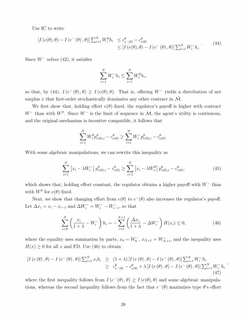
Use IC to write

[I (e(θ), θ)− I (e− (θ) , θ)]∑N

i=1Wθi hi ≤ cθe−(θ) − cθe(θ)

≤ [I (e(θ), θ)− I (e− (θ) , θ)]∑N

i=1 W−i hi

. (44)

Since W− solves (42), it satisfies

N∑i=1

W−i hi ≤

N∑i=1

W θi hi,

so that, by (44), I (e− (θ) , θ) ≥ I (e(θ), θ). That is, offering W− yields a distribution of netsurplus x that first-order stochastically dominates any other contract in M.

We first show that, holding effort e(θ) fixed, the regulator’s payoff is higher with contractW− than with W θ. Since W− is the limit of sequence in M, the agent’s utility is continuous,and the original mechanism is incentive compatible, it follows that

N∑i=1

W θi p

θe(θ),i − cθe(θ) ≥

N∑i=1

W−i p

θe(θ),i − cθe(θ).

With some algebraic manipulations, we can rewrite this inequality as

N∑i=1

[xi − λW−

i

]pθe(θ),i − cθe(θ) ≥

N∑i=1

[xi − λW θ

i

]pθe(θ),i − cθe(θ), (45)

which shows that, holding effort constant, the regulator obtains a higher payoff with W− thanwith W θ for e(θ) fixed.

Next, we show that changing effort from e(θ) to e−(θ) also increases the regulator’s payoff.Let ∆xi = xi − xi−1 and ∆W−

i = W−i −W−

i−1, so that

N∑i=0

(xi

1 + λ−W−

i

)hi = −

N+1∑i=1

(∆xi

1 + λ−∆W−

i

)H(xi) ≤ 0, (46)

where the equality uses summation by parts, x0 = W−0 , xN+1 = W−

N+1, and the inequality usesH(x) ≥ 0 for all x and FD. Use (46) to obtain:

[I (e (θ) , θ)− I (e− (θ) , θ)]∑N

i=1 xihi ≥ (1 + λ) [I (e (θ) , θ)− I (e− (θ) , θ)]∑N

i=1 W−i hi

≥ cθe−(θ) − cθe(θ) + λ [I (e (θ) , θ)− I (e− (θ) , θ)]∑N

i=1 W−i hi

,

(47)where the first inequality follows from I (e− (θ) , θ) ≥ I (e(θ), θ) and some algebraic manipula-tions, whereas the second inequality follows from the fact that e−(θ) maximizes type θ’s effort

38

under contract W− (program 43). Rearranging (47), we obtain:

−[I(e− (θ) , θ

)− I (e (θ) , θ)

] N∑i=1

[xi − λW−

i

]hi ≥ cθe−(θ) − cθe(θ).

Using MS, this inequality can be written as

N∑i=1

(xi − λW−

i

)pθe−(θ),i − cθe−(θ) ≥

N∑i=1

(xi − λW−

i

)pθe(θ),i − cθe(θ), (48)

which establishes that the change in effort from e(θ) to e−(θ) increases the regulator’s payoff.Combining inequalities (45) and (48) concludes the proof.Part b) As in the proof of Theorem 3, let hi ≡ H (xi+1) − H (xi) and, with a slight abuse ofnotation, write pθe,i for pθe(xi) and Wi for W (xi). If (W, e) is an optimal monotone mechanism,it must solve the following program

min{Wi}

N∑i=1

Wi

ˆΘ

pθe(θ),idµ(θ)

subject toN∑i=1

Wihi = K, (IC’)

Wi ≥ 0, (LL)

xi − xi−1

1 + λ≥ Wi −Wi−1. (M)

Using the same arguments as in proof of Theorem 3, it follows that there exists x such that

w(x) =

{0 if x ≤ xx−x1+λ

if x > x.

Rewriting in terms of costs, we obtain w(C) = max{C − C; 0

}, where C ≡ S−x

1+λ.

B. Examples

Screening with Pure Adverse Selection (continuation)

Given a high effort, the probability of success for type A is pA1 = 23and for type B is pB1 = 1

3. We

assume that the project fails with a high enough probability if they exert low effort and we takexH − xL to be large enough for the principal to want to implement high effort from both types.

39

Let wij denote type i’s payment in state j. The optimal mechanism must solve the followingprogram:

minwiH ,w

iL≥0

2wAH + wAL + wBH + 2wBL

subject to 2wAH + wAL ≥ 2wBH + wBLwBH + 2wBL ≥ wAH + 2wAL2wAH + wAL ≥ 3

wBH + 2wBL ≥ 2.

The two first constraints require A and B to prefer to report their types truthfully (IC con-straints). Because effort is observable, the principal does not need to worry about deviations oneffort. Then, it is no longer the case that LL implies IR. The last two constraints are preciselythe IR constraints.

Example 2 (continuation)

Consider the relaxed program:

minwji≥0

N∑i=1

µiwii

2

subject to1

2

(wii +

∑j 6=iw

ji

N

)≥ 1.

This is a relaxed program in that it only considers the “pure moral hazard” ICs. The solution is

wθ (xi) =

{2 if x = xθ

0 if x 6= xθ.

The proof concludes by verifying that this solution satisfies the omitted ICs. The ICs preventingeach type from deviating in both effort and contracts are satisfied with equality:

0 =1

2· 2− 1 = wi0 = 0.

The ICs preventing each type from picking a different contracts while exerting high effort holdwith inequality:

0 =1

2· 2− 1 >

1

N· 2− 1.

Thus, all omitted ICs are satisfied.

40

C. Multiplicative Separability

This appendix examines the multiplicative separability condition (MS). We provide two results.The first is a characterization of MS in terms of the ordering of incentives. The second one is agraphical interpretation of how distributions satisfying MS change with effort.

Recall the condition presented in the text, which allows contracts to be ranked by theirincentives:

Definition 3. A distribution of outputs is ordered in terms of incentives if, for any w and w

satisfying LL,N∑i=1

w(xi)(pθ0e0(xi)− p

θ0e0

(xi))

=N∑i=1

w(xi)(pθ0e0(xi)− p

θ0e0

(xi))

for some e0, e0 ∈ E and θ0 ∈ Θ, then

N∑i=1

w(xi)(pθe(xi)− pθe(xi)

)=

N∑i=1

w(xi)(pθe(xi)− pθe(xi)

)for all θ ∈ Θ and e, e ∈ E.

Substitution shows that any distribution that satisfies MS must be ordered in terms ofincentives. The next proposition shows that the reverse is also true, so these are equivalentconditions:

Proposition 3. The following statements are equivalent:1. The distribution of outputs pθe(x) is ordered in terms of incentives.2. The distribution of outputs pθe(x) satisfies MS.3. For all i, j, there exist constants φi,j (that depend on the outputs xi and xj but not on

type or effort) such thatpθe(xi)− pθe(xi)pθe(xj)− pθe(xj)

= φi,j (49)

whenever pθe(xj)− pθe(xj) 6= 0.

Proof. We first show the equivalence between (2) and (3). From Definition 1, a distributionsatisfies MS if and only if, for all (x, θ, e, e),

pθe(x)− pθe(x) = [I(e, θ)− I(e, θ)]H(x). (50)

Since (2) and (3) trivially hold if pθe(xi) = pθe(xi) for all x, θ, e, and e, it suffices to consider thecase where pθe(xj) 6= pθe(xj) for some (xj, θ, e, e).

41

Suppose MS holds. Then, we must have H(xj) 6= 0. Multiplying both sides of equation (50)by H(xi)

H(xj), we obtain:

[pθe(xj)− pθe(xj)

] H(xi)

H(xj)= [I(e, θ)− I(e, θ)]H(xi) = pθe(xi)− pθe(xi).

Setting φi,j ≡ H(xi)H(xj)

establishes the equation in the statement. Conversely, when property (3)does not hold, it is impossible to find H and I that satisfy (50).

Next, we establish that (3) implies (1). To do so, suppose that (3) holds, and let w and wbe two payment vectors satisfying LL such that

N∑i=1

w(xi)[pθ0e0

(xi)− pθ0e0(xi)] =N∑i=1

w(xi)[pθ0e0

(xi)− pθ0e0(xi)] (51)

for some e0, e0 ∈ E and θ0 ∈ Θ. Without loss of generality, suppose that pθ0e0(xj) 6= pθ0e0(xj)

for some (xj, θ0, e0, e0) (the distribution would immediately be ordered in terms of incentives ifpθe(xi) = pθe(xi) for all (xi, θ, e, e). For notational simplicity (relabeling if needed), let j = 1.

Use equation (49) to write:

N∑i=1

w(xi)[pθ0e0

(xi)− pθ0e0(xi)] = [pθ0e0(x1)− pθ0e0(x1)]N∑i=1

w(xi)φi,1,

andN∑i=1

w(xi)[pθ0e0

(xi)− pθ0e0(xi)] = [pθ0e0(x1)− pθ0e0(x1)]N∑i=1

w(xi)φi,1.

Substitute these equations in (51):

[pθ0e0(x1)− pθ0e0(x1)]N∑i=1

w(xi)φi,1 = [pθ0e0(x1)− pθ0e0(x1)]N∑i=1

w(xi)φi,1,

which, since pθ0e0(x1) 6= pθ0e0(x1), implies:

N∑i=1

w(xi)φi,1 =N∑i=1

w(xi)φi,1.

For each θ, e, and e, multiply both sides by pθe(x1)− pθe(x1) to obtain:

[pθe(x1)− pθe(x1)]N∑i=1

w(xi)φi,1 = [pθe(x1)− pθe(x1)]N∑i=1

w(xi)φi,1.

42

Then, using condition (49) again, gives:

N∑i=1

w(xi)[pθe(xi)− pθe(xi)] =

N∑i=1

w(xi)[pθe(xi)− pθe(xi)],

which establishes (1).It remains to show that (1) implies in (3). Notice that if a distribution is ordered in terms

of incentives, then either pθe(·)− pθe(·) is identical to zero for each θ, e, and e, which immediatelyimplies condition (49), or there exists a non-null vector pθ0e0(·) − p

θ0e0

(·), for some θ0, e0 and e0,such that

{w ∈ RN ;w · (pθ0e0 − pθ0e0

) = 0} ⊂ {w ∈ RN ;w · (pθe − pθe) = 0},

for all θ, e and e, where · represents the canonical inner product of RN . Therefore, the orthogonalcomplement of pθe−pθe in RN contains the orthogonal complement of pθ0e0−p

θ0e0, which means that

pθe − pθe is collinear to pθ0e0 − pθ0e0

for all θ, e and e. Therefore,

pθe(xi)− pθe(xi) = φi,j(pθe(xj)− pθe(xj)

)where

φi,j =pθ0e0(xi)− p

θ0e0

(xi)

pθ0e0(xj)− pθ0e0(xj)

for pθ0e0(xj)− pθ0e0

(xj) 6= 0.

Proposition 3 shows the equivalence between three properties of a probability distribution.As discussed in the main text, property (1) states that if one type has the same incentives toexert two efforts under contracts w and w, so do all other types. In other words, all contractscan be ranked in terms of the incentives that they provide. Property 2 is the MS condition usedin the text.

Property 3 provides a straightforward graphic interpretation of what it means for a dis-tribution to be multiplicatively separable. It means that, for all types, changing effort has aproportional effect on the probability of each outcome. For example, suppose there are threeoutputs so that the probabilities conditional on each type and effort lie on the two-dimensionalsimplex. Because probabilities add up to 1, one of the equalities in (49) is redundant, and adistribution satisfies MS if and only if

pθe(x2)− pθe(x2) = φ[pθe(x3)− pθe(x3)

]for some constant φ. This condition is represented in Figure 1. Each point is the graph corre-sponds to the probability distribution conditional on a type and an effort. We draw two points

43

Figure 1: Multiplicative Separability with three outputs.

with the same color if they correspond to the same type but different efforts. MS requires thelines connecting these points to have the same slope (φ).

D. Generalized Multiplicative Separability

Definition 4. Let (T , ω) be finite probability space. The distribution of outputs satisfies gen-eralized multiplicative separability (GMS) if there exist a function H : X × T → R+ andmeasurable function I : E ×Θ× T → R such that

F θe (x) +

T∑t=1

H (x, t) I(e, θ, t)ωt = F θe (x) +

T∑t=1

H (x, t) I (e, θ, t)ωt, ∀e, e, θ, x, (GMS)

andI(e, θ, t) ≥ I(e, θ, t)⇐⇒ I(e, θ, t) ≥ I(e, θ, t)

for all e, e, t, t, θ.

Example 3. We say that the distribution of outputs satisfies the Generalized Linearity of theDistribution Function Condition if

F θe (x) =

T∑t=0

I(e, θ, t)Ft(x) = −T∑t=1

I(e, θ, t)H(x, t) + F0(x), (52)

where{Ft(x); t = 1, ..., T

}is a family of cumulative distributions, I(e, θ, t) ≥ 0,

∑Tt=1 I(e, θ, t) =

1 and H(x, t) = F0(x) − Ft(x). If E = [0, 1], Ft first-order stochastically dominates F0 and

44

I(·, θ, t) is non-decreasing for all t and θ, then the distribution of outputs satisfies GMS.

Theorem 4. Suppose that GMS holds. There exists an optimal mechanism that offers a singlecontract to all types. Moreover, for any optimal mechanism, there exists an equivalent mechanismthat offers a single contract.

Proof. By Lemma 6, there is no loss of generality in assuming that all contracts are uniformlybounded. By GMS, a type-θ agent who switches from effort e to e while keeping the samecontract w gains

vθe(w)− vθe(w) =T∑t=1

[I(e, θ, t)− I(e, θ, t)]N∑i=1

wihi(t)ωt + cθe − cθe. (53)

In turn, this switch changes the principal’s payoff by

uθe(w)− uθe(w) =T∑t=1

[I(e, θ, t)− I(e, θ, t)]N∑i=1

[xi − wi]hi(t)ωt. (54)

Let (w, e) be a feasible mechanism. The set of all bonuses in this mechanism,

M :={wθ : θ ∈ Θ

},

is well defined and is composed of uniformly bounded functions. Therefore, its closureM is acompact set.

Let w∗ be a solution of the following maximization program:

maxw∈M,t∈T

N∑i=1

wihi(t). (55)

Since M is compact and S is finite, the objective function is a continuous linear functionaland the constraint defines a closed set, (55) has a solution w∗ ∈ M.

Let e∗(θ) be an effort that maximizes the agent’s payoff under contract w∗:

vθe∗(θ)(w∗) ≥ vθe(θ)(w

∗),

which, by GMS, can be written as

T∑t=1

[I(e(θ), θ, t)− I(e∗(θ), θ, t)]N∑i=1

w∗i hi (t)ωt ≥ cθe∗(θ) − cθe(θ). (56)

45

Similarly, because e(θ) is his effort choice with contract wθ(x),

T∑t=1

[I(e(θ), θ, t)− I(e∗(θ), θ, t)]N∑i=1

wθi hi (t)ωt ≤ cθe∗(θ) − cθe(θ). (57)

Combining (56) and (57), we obtain

∑Tt=1 [I(e(θ), θ, t)− I(e∗(θ), θ, t)]

∑Ni=1w

θi hi (t)ωt ≤ cθe∗(θ) − cθe(θ) ≤∑T

t=1 [I(e(θ), θ, t)− I(e∗(θ), θ, t)]∑N

i=1w∗i hi (t)ωt.

(58)

Since w∗ solves program (55), we have

N∑i=1

w∗i hi(t) ≥N∑i=1

wθi hi(t), for all t ∈ T .

Therefore, it follows from GMS and (58) that I(e(θ), θ, t) ≥ I(e∗(θ), θ, t), for all t ∈ T .We now establish that replacing contract wθ by w∗ increases the principal’s payoff from type

θ. As in the proof of Theorem 2, we first show that, holding effort fixed, the principal is betteroff with the substitution of contracts. Since w∗ is the limit of sequence inM, the agent’s utilityis continuous, and the original mechanism is incentive compatible, it follows that

vθe(θ)(wθ) ≥ vθe(θ)(w

∗). (59)

Multiply both sides by −1 and add∑N

i=0 xipθe(θ),i to both sides of this inequality to obtain:

N∑i=1

[xi − w∗i ] pθe(θ),i ≥N∑i=1

[xi − wθi

]pθe(θ),i, (60)

which states that, holding effort e(θ) fixed, the principal gets a higher profit with contract w∗

than with wθ.Next, we show that the change in effort also benefits the principal. Notice first that FD

implies that the function x → x − w∗(x) is non-decreasing. Therefore, applying integration byparts and using GMS and FD, we conclude that

N∑i=0

[xi − w∗i ]hi(t) = −N+1∑i=1

[∆xi −∆w∗i ]H(xi, t) ≤ 0, for all t,

where ∆xi = xi − xi−1, ∆w∗i = w∗i − w∗i−1 and x0 = w∗0 and xN+1 = w∗N+1. Hence, since

46

I(e(θ), θ, t) ≥ I(e∗(θ), θ, t), for all t, we have that

[I(e(θ), θ, t)− I(e∗(θ), θ, t)]N∑i=1

[xi − w∗i ]hi (t) ≤ 0, for all t.

Using again GMS, we can rewrite this last inequality as

N∑i=1

[xi − w∗i ]pθe∗(θ),i ≥N∑i=1

[xi − w∗i ] pθe(θ),i, (61)

which shows that the principal gains from the change in effort.Combining (60) and (61) establishes that the principal’s profit from θ with the new contract

exceeds her profit with the original contract:

uθe∗(θ)(w∗) ≥ uθe(θ)(w

θ).

Consider the mechanism (w, e): wθ(x) = w∗(θ) and e(θ) = e∗(θ), where e∗(θ) ∈ arg maxe

vθe(w∗),

for all θ. As previously shown, this mechanism raises the principal’s payoff pointwise and satisfiesLL. Notice that the expected utility of type θ at contract w∗ who chooses effort e is

vθe(w∗) =

N∑i=1

w∗i pθe,i − cθe.

Since w∗ ≥ 0 and the agent must weakly prefer the recommended effort e∗ to the one with cθe ≤ 0,the IR constraint must hold. Since the mechanism (w, e) is constituted by only one contract, ittrivially satisfies IC. The proof of the second part is analogous to the proof from Theorem 2.

References

Bajari, P. and S. Tadelis (2001): “Incentives Versus Transaction Costs: A Theory of Pro-curement Contracts,” RAND Journal of Economics, 32, 287–307.

Biais, B. and T. Mariotti (2005): “Strategic Liquidity Supply and Security Design,” Reviewof Economic Studies, 72, 615–649.

Burguet, R., J.-J. Ganuza, and E. Hauk (2012): “Limited Liability and Mechanism Designin Procurement,” Games and Economic Behavior, 76, 15–25.

Caillaud, B., R. Guesnerie, and P. Rey (1992): “Noisy Observation in Adverse SelectionModels,” Review of Economic Studies, 59, 595–615.

47

Carroll, G. (Forthcoming): “Robustness and Linear Contracts,” American Economic Review.

Chaigneau, P., A. Edmans, and D. Gottlieb (2014): “The Value of Informativeness forContracting,” Tech. rep., HEC Montreal, LBS, and Wharton.

Chassang, S. (2013): “Calibrated Incentive Contracts,” Econometrica, 81, 1935–1971.

Chiappori, P.-A. and B. Salanie (2003): “Testing Contract Theory: A Survey of SomeRecent Work,” in Advances in Economics and Econometrics, ed. by M. Dewatripont, L. P.Hansen, and S. T. Turnovsky, Cambridge: Cambridge University Press, vol. 1.

Chu, L. Y. and D. Sappington (2007): “Simple Cost-Sharing Contracts,” American Eco-nomic Review, 97, 419–428.

Demarzo, P. and D. Duffie (1999): “A Liquidity-based Model of Security Design,” Econo-metrica, 67, 65–99.

DeMarzo, P. M. (2005): “The Pooling and Tranching of Securities: A Model of InformedIntermediation,” Review of Financial Studies, 18, 1–35.

DeMarzo, P. M., I. Kremer, and A. Skrzypacz (2005): “Bidding with Securities: Auctionsand Security Design,” American Economic Review, 95, 936–959.

Dewatripont, M., P. Legros, and S. A. Matthews (2003): “Moral Hazard and CapitalStructure Dynamics,” Journal of the European Economic Association, 1, 890–930.

Edmans, A. and X. Gabaix (2011): “Tractability in Incentive Contracting,” Review of Fi-nancial Studies, 24, 2865–94.

Farhi, E. and J. Tirole (Forthcoming): “Liquid Bundles,” Journal of Economic Theory.

Gottlieb, D. and H. Moreira (2014): “Simultaneous Adverse Selection and Moral Hazard,”Tech. rep., Wharton School and EPGE/FGV.

Grossman, S. J. and O. D. Hart (1983): “An Analysis of the Principal-Agent Problem,”Econometrica, 51, 7–45.

Guesnerie, R. and J.-J. Laffont (1984): “A Complete Solution to a Class of Principal-Agent Problems with an Application to the Control of a Self-Managed Firm,” Journal ofPublic Economics, 25, 329–369.

Hart, O. D. and B. Holmstrom (1987): “The Theory of Contracts,” in Advances in EconomicTheory, Fifth World Congress, ed. by T. Bewley, Cambridge: Cambridge University Press.

48

Holmstrom, B. (1979): “Moral Hazard and Observability,” The Bell Journal of Economics,10, 74–91.

Holmstrom, B. and P. Milgrom (1987): “Aggregation and Linearity in the Provision ofIntertemporal Incentives,” Econometrica, 55, 303–28.

Innes, R. D. (1990): “Limited Liability and Incentive Contracting with Ex-Ante ActionChoices,” Journal of Economic Theory, 52, 45–67.

Jewitt, I., O. Kadan, and J. M. Swinkels (2008): “Moral Hazard with Bounded Payments,”Journal of Economic Theory, 143, 59–82.

Laffont, J.-J. and D. Martimort (2002): The Theory of Incentives: The Principal-AgentModel, Princeton University Press.

Laffont, J.-J. and J. Tirole (1986): “Using Cost Observation to Regulate Firms,” Journalof Political Economy, 94, 614–641.

——— (1993): A Theory of Incentives in Procurement and Regulation, MIT press.

Matthews, S. A. (2001): “Renegotiating Moral Hazard Contracts under Limited Liability andMonotonicity,” Journal of Economic Theory, 97, 1–29.

Melumad, N. D. and S. Reichelstein (1989): “Value of Communication in Agencies,”Journal of Economic Theory, 47, 334–368.

Nachman, D. C. and T. H. Noe (1994): “Optimal design of securities under asymmetricinformation,” Review of Financial Studies, 7, 1–44.

Ollier, S. and L. Thomas (2013): “Ex Post Participation Constraint in a Principal–AgentModel with Adverse Selection and Moral Hazard,” Journal of Economic Theory, 148, 2383–2403.

Page, F. H. (1992): “Mechanism Design for General Screening Problems with Moral Hazard,”Economic Theory, 2, 265–281.

Picard, P. (1987): “On the Design of Incentive Schemes under Moral Hazard and AdverseSelection,” Journal of Public Economics, 33, 305–31.

Poblete, J. and D. Spulber (2012): “The Form of Incentive Contracts: Agency with MoralHazard, Risk Neutrality, and Limited Liability,” RAND Journal of Economics, 43, 215–34.

Rochet, J.-C. and L. A. Stole (2002): “Nonlinear Pricing with Random Participation,”Review of Economic Studies, 69, 277–311.

49

Rogerson, W. P. (2003): “Simple Menus of Contracts in Cost-Based Procurement and Regu-lation,” American Economic Review, 93, 919–26.

Tirole, J. (2005): The Theory of Corporate Finance, Princeton University Press.

50

Online Appendix

Existence

This proof covers the model with two outputs as a particular case. By Lemma 6, there is no lossof generality in taking uniformly bounded contracts. Let L > 0 denote this uniform bound sothat W := [0, L]N ⊂ RN denotes the space of contracts. Let B(W) be the Borel σ-field in W .

Let vθe(w) :=∑N

i=1w(xi)pθe(xi) − cθe. By Assumption 2, vθ· (·) is continuous on W × E, and,

for each (w, e) ∈ W × E, v·e(w) is B(Θ)-measurable. Since E is compact and vθ· (w) continuous,the agent’s effort choice problem has a solution. Let V θ(w) := sup

e∈Evθe(w) denote the utility

of type θ. Let the non-empty, compact-valued mapping (θ, w) → e∗(θ, w) denote the “reactionfunction” of type θ:

e∗(θ, w) := {e ∈ E : vθe(w) ≥ V θ(w)}.

By Berge’s Maximum Theorem, w → V θ(w) is continuous for each θ and w → e∗(θ, w) is uppersemicontinuous on W for each θ.

Let uθe(w) :=∑N

i=1[xi−w(xi)]pθe(xi) denote the principal’s payoff. By Assumption 2, for each

θ ∈ Θ, uθ· (·) is continuous on W × E, and for each (w, e) ∈ W × E, u·e(w) is B(Θ)-measurable.Notice that p is µ-integrable on Θ× E because |pθe| ≤ 1 on Θ× E.

Since e∗(θ, w) is compact and uθ· (w) continuous, for each (θ, w), the problem supe∈e∗(θ,w)

uθe(w)

has a solution, say eθw. Thus, for each contract w, the principal can provide the agent with alist, {eθw; θ ∈ Θ}, of recommended efforts. Since eθw ∈ e∗(θ, w) for each θ ∈ Θ, a type-θ agent hasno incentive to take an effort other than the one requested by the principal eθw (i.e., the agent isobedient). To choose the best list of requests, the principal must therefore solve the problem

supe∈e∗(θ,w)

uθe(w)

for each (θ, w) ∈ Θ×W . Let U θ(w) := supe∈e∗(θ,w)

uθe(w). Since u is B(Θ)×B(W)×B(E)-measurable

and continuous on E, and since e∗(·, ·) is B(Θ)×B(W)-measurable (see Nowak (1984), Lemma1.10) and compact-valued, it follows that U is B(Θ)×B(W)-measurable (see Himmelberg et.al.(1976), Theorem 2). Moreover, since e∗(θ, ·) is upper semicontinuous on W , it follows fromTheorem 2 of Berge (1963) that U θ(·) is upper semicontinuous on W for each θ. Finally, sincethe principal’s payoff u is integrably bounded, U : Θ ×W → R is also integrably bounded onΘ×W .

With these observations, we can write the principal’s program as

supw∈W

ˆU θ(w)dµ(θ)

51

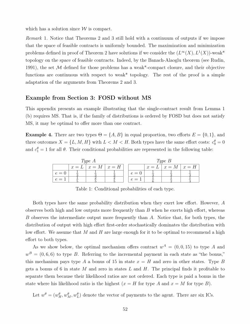
which has a solution since W is compact.

Remark 1. Notice that Theorems 2 and 3 still hold with a continuum of outputs if we imposethat the space of feasible contracts is uniformly bounded. The maximization and minimizationproblems defined in proof of Theorem 2 have solutions if we consider the (L∞(X), L1(X))-weak*topology on the space of feasible contracts. Indeed, by the Banach-Alaoglu theorem (see Rudin,1991), the setM defined for those problems has a weak*-compact closure, and their objectivefunctions are continuous with respect to weak* topology. The rest of the proof is a simpleadaptation of the arguments from Theorems 2 and 3.

Example from Section 3: FOSD without MS

This appendix presents an example illustrating that the single-contract result from Lemma 1(b) requires MS. That is, if the family of distributions is ordered by FOSD but does not satisfyMS, it may be optimal to offer more than one contract.

Example 4. There are two types Θ = {A,B} in equal proportion, two efforts E = {0, 1}, andthree outcomes X = {L,M,H} with L < M < H. Both types have the same effort costs: cθ0 = 0

and cθ1 = 1 for all θ. Their conditional probabilities are represented in the following table:

Type Ax = L x = M x = H

e = 0 13

13

13

e = 1 15

25

25

Type Bx = L x = M x = H

e = 0 13

13

13

e = 1 16

12

13

Table 1: Conditional probabilities of each type.

Both types have the same probability distribution when they exert low effort. However, Aobserves both high and low outputs more frequently than B when he exerts high effort, whereasB observes the intermediate output more frequently than A. Notice that, for both types, thedistribution of output with high effort first-order stochastically dominates the distribution withlow effort. We assume that M and H are large enough for it to be optimal to recommend a higheffort to both types.

As we show below, the optimal mechanism offers contract wA = (0, 0, 15) to type A andwB = (0, 6, 6) to type B. Referring to the incremental payment in each state as “the bonus,”this mechanism pays type A a bonus of 15 in state x = H and zero in other states. Type Bgets a bonus of 6 in state M and zero in states L and H. The principal finds it profitable toseparate them because their likelihood ratios are not ordered. Each type is paid a bonus in thestate where his likelihood ratio is the highest (x = H for type A and x = M for type B).

Let wθ = (wθH , wθM , w

θL) denote the vector of payments to the agent. There are six ICs.

52

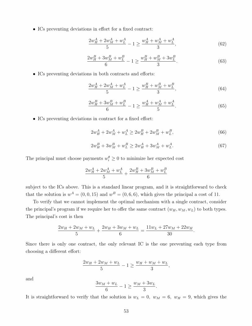
• ICs preventing deviations in effort for a fixed contract:

2wAH + 2wAM + wAL5

− 1 ≥ wAH + wAM + wAL3

, (62)

2wBH + 3wBM + wBL6

− 1 ≥ wBH + wBM + 3wBL3

. (63)

• ICs preventing deviations in both contracts and efforts:

2wAH + 2wAM + wAL5

− 1 ≥ wBH + wBM + wBL3

, (64)

2wBH + 3wBM + wBL6

− 1 ≥ wAH + wAM + wAL5

. (65)

• ICs preventing deviations in contract for a fixed effort:

2wAH + 2wAM + wAL ≥ 2wBH + 2wBM + wBL , (66)

2wBH + 3wBM + wBL ≥ 2wAH + 3wAM + wAL . (67)

The principal must choose payments wθi ≥ 0 to minimize her expected cost

2wAH + 2wAM + wAL5

+2wBH + 3wBM + wBL

6

subject to the ICs above. This is a standard linear program, and it is straightforward to checkthat the solution is wA = (0, 0, 15) and wB = (0, 6, 6), which gives the principal a cost of 11.

To verify that we cannot implement the optimal mechanism with a single contract, considerthe principal’s program if we require her to offer the same contract (wH , wM , wL) to both types.The principal’s cost is then

2wH + 2wM + wL5

+2wH + 3wM + wL

6=

11wL + 27wM + 22wH30

.

Since there is only one contract, the only relevant IC is the one preventing each type fromchoosing a different effort:

2wH + 2wM + wL5

− 1 ≥ wH + wM + wL3

,

and3wM + wL

6− 1 ≥ wM + 3wL

3.

It is straightforward to verify that the solution is wL = 0, wM = 6, wH = 9, which gives the

53

principal a cost of 12. Thus, offering the best single-contract mechanism yields a higher costthan offering the optimal menu of contracts in this example.

References

Berge, C. (1963). Topological Spaces. MacMillan: New York.

Himmelberg, C.J., Parthasarathy, T. and VanVleck, F.S. (1976), “Optimal plansfor dynamic programming problems,” Mathematics of Operations Research, Mathematicsof Operations Research, 1, pp. 390-394.

Nowak, A.S. (1984), “On zero-sum stochastic games with general state space.I,” Proba-bility and Mathematical Statistics, 4(1), pp. 13-32.

Rudin, W. (1991). Functional Analysis. McGraw-Hill: New York., 2nd edition.

54