Embed Size (px)
Citation preview
Simple Contracts for Reliable Supply:Capacity Versus Yield Uncertainty*
Woonam HwangManagement Science and Operations, London Business School, [email protected]
Nitin BakshiManagement Science and Operations, London Business School, [email protected]
Victor DeMiguelManagement Science and Operations, London Business School, [email protected]
Events such as labor strikes and natural disasters, and yield losses from manufacturing defects, have a sub-
stantial impact on supply reliability. Importantly, suppliers can mitigate this supply risk by improving their
processes or overproducing, but their mitigating actions are often not directly contractible. We investigate
when and why the simple wholesale price contract performs well in such settings. We find that supply chain
profit (or equivalently, efficiency) is essentially determined by supply reliability, which in turn depends on
three factors: (i) the type of supply risk (whether the supplier’s capacity is random or the supplier’s yield is
random), (ii) the relative bargaining power of the buyer and the supplier, and (iii) whether the buyer or the
supplier determines the production quantity decision. We find that, although suboptimal, simple contracts
can often generate high efficiency. For random capacity, simple contracts perform well when the supplier is
powerful. Surprisingly, for random yield, when the buyer controls the production quantity decision, simple
contracts perform well when the buyer is powerful. If the buyer delegates the production decision to the
supplier, then simple contracts perform well when either party is powerful. Finally, we find that, for random
yield, simple contracts generally perform better under delegation than under control.
Key words : supplier reliability, random capacity, random yield, simple contracts, delegation
History : September 27, 2014
1. Introduction
In an era of outsourcing and globalization, reliability of supply is an increasingly important aspect
of supply-chain management. Hendricks and Singhal (2005a,b) provide empirical evidence for the
dramatic impact of supply disruptions on firm stock returns and operating performance. Supply
disruptions are often classified as either random capacity or random yield ; Wang et al. (2010).
Random capacity disruptions affect the supplier’s production capacity; e.g., due to natural disasters
* We are grateful to Nitish Jain for his help in the analysis, and also grateful for comments from Volodymyr Babich,Gerard Cachon, Nicole DeHoratius, Jeremie Gallien, Sang-Hyun Kim, Serguei Netessine, Ozalp Ozer, Kamalini Ram-das, Nicos Savva, Dongyuan Zhan, and seminar participants at the 2012 MSOM Conference in New York, the 2012INFORMS Annual Meeting in Phoenix, the 2013 Trans-Atlantic Doctoral Conference in London, the 2013 MSOMConference in Fontainebleau, the 2013 INFORMS Annual Meeting in Minneapolis, the 2014 POMS Conference inAtlanta, the 2014 MSOM Conference in Seattle, the 2014 IFORS Conference in Barcelona, the Judge Business Schoolat University of Cambridge, and the McDonough School of Business at Georgetown University.
1
2 Hwang, Bakshi, and DeMiguel: Simple Contracts for Reliable Supply
such as the tsunami in Japan, which temporarily wiped out the capacity of key suppliers to Toyota
(New York Times 2011), or due to labor strikes, such as those that broke out in factories across
China following worker suicides at Foxconn, a key supplier to Apple and HP (The Wall Street
Journal 2010). Random yield disruptions, on the other hand, affect the supplier’s production yield;
e.g., when manufacturers of biopharmaceuticals, high-tech electronics, or semiconductors suffer
from manufacturing defects. For instance, Bohn and Terwiesch (1999) point to evidence that high-
tech manufacturers such as Seagate experience production yields as low as 50%.
Critically, suppliers can often exert ex-ante effort to improve their reliability. For random capacity
disruptions, suppliers may invest in robust plans for disaster recovery and business continuity
(The Wall Street Journal 2012, New York Times 2009). Lexology (2010) describes the proactive
measures firms could undertake to avoid labor strikes such as periodically reviewing compliance
with labor regulations, being prudent in wage negotiations, and embracing a culture of partnership
between labor and management. For random yield disruptions also, the supplier’s effort can have a
substantial impact on improving yields in various manufacturing contexts. For instance, Snow et al.
(2006) provide an excellent discussion about Genentech’s cell culture production, and explain how
suppliers can improve their yield not only through ongoing R&D but also by “protecting against
contamination by monitoring the raw materials, limiting human involvement in production, testing
frequently, and ensuring that all connections between pieces of equipment were tightly sealed.”
Process-improving effort is costly and often non-contractible. For instance, in our conversations
with Samsung’s semiconductor foundry, we learnt that improving yield is a key focus in the pro-
duction process, but the specifics of how to do so are not contractible.1 This exposes the buyer to
moral hazard,2 and due to the resulting agency issues, the supplier may shirk on effort, thereby
leading to potentially severe disruptions.3 Yet, much of the existing academic literature assumes
that reliability is exogenous. Also, the few papers that capture endogenous reliability rely on the
assumption that either the buyer is responsible for process improvement, or that the supplier’s
efforts are directly contractible.
In this manuscript, we consider the case in which reliability is endogenous and the supplier’s
mitigating actions are non-contractible, and study the motivation of the supplier to improve his
1 A decision is not contractible, for instance, when the decision is either unobservable or too costly to verify in a courtof law.
2 Note that we use the term moral hazard in the general sense of an economic agent possessing insufficient incentivesto exert care, and we do not make any a priori supposition about the allocation of bargaining power between thecounter-parties (Rowell and Connelly 2012, Pitchford 1998). This is subtly different from the more typical, albeitnarrower, usage of moral hazard in principal–agent relationships, wherein the principal possesses all the bargainingpower.
3 Recently, a spate of fires in garment factories in Bangladesh has been attributed to poor maintenance of electricalwiring and “severe negligence” on the part of the factory owners (BBC 2012).

Hwang, Bakshi, and DeMiguel: Simple Contracts for Reliable Supply 3
reliability. Complex contracts may be used to align the incentives of the buyer and the supplier and
improve reliability, but a recurring theme from a real-world perspective is the widespread use of
the simple linear wholesale price contract.4 Therefore, our main research question is to understand
under which circumstances the simple linear wholesale price contract suffices to achieve supply
reliability (and hence, high supply chain profit) and when complex contracts are required. To
answer this question, we model a supply chain with one buyer and one supplier transacting over a
single period.
For random yield, reliability can be improved not only by investing in process improvement
but also by inflating the production quantity, thus creating a buffer against yield losses. Hence,
an additional dimension of moral hazard may emerge depending on whether the buyer or the
supplier decides the production quantity. Specifically, we consider two scenarios: i) Control, in
which the buyer controls or determines the production quantity (i.e., only the buyer inflates); and
ii) Delegation, in which the supplier determines the production quantity (i.e., both parties can
inflate). Our main findings are as follows.
With respect to the performance of the wholesale price contract, we find that three factors—the
type of supply risk, the bargaining power of buyer and supplier, and whether the buyer or the
supplier decides the production quantity—jointly determine when the simple linear wholesale price
contract leads to high supply-chain efficiency and when more complex contracts are warranted.5
For random capacity, the efficiency of the wholesale price contract is monotonically increasing
in wholesale price and, therefore, in the supplier’s bargaining power.6 The reason is that a more
powerful supplier (higher wholesale price) has a bigger margin, and therefore, has a greater incentive
to invest effort, and thereby improve efficiency. This suggests that the wholesale price contract
may be preferred over more complex contracts (which theoretically perform better but are costly
to administer) if the supplier is “powerful”.
In contrast, for random yield, when the buyer controls the production quantity decision, the
monotonicity trend in efficiency generated by the wholesale price contract is reversed. As before,
a higher wholesale price increases the supplier’s incentive to invest in reliability, but now it also
reduces the buyer’s incentive to inflate her order quantity. Moreover, the order quantity plays a dual
4 Papers that restrict attention to the wholesale price contract include Lariviere and Porteus (2001), Cachon (2004),Perakis and Roels (2007), Federgruen and Yang (2009a), Babich et al. (2007), and the references therein. In thisstrand of literature, the popularity of the wholesale price contract has essentially been attributed to its simplicity.Specifically, the literature puts forth two reasons why simple contracts are preferred in practice: (i) they are easierto design and negotiate (Kalkancı et al. 2011, 2014), and (ii) they are easier to enforce legally (Schwartz and Watson2004).
5 Supply-chain efficiency is defined as the ratio of the expected profit of the decentralized supply chain to the optimalexpected profit in the centralized supply chain.
6 A higher wholesale price is consistent with greater bargaining power for the supplier since his payoff is increasingin wholesale price, while the buyer’s payoff is decreasing.
4 Hwang, Bakshi, and DeMiguel: Simple Contracts for Reliable Supply
role by directly influencing proportional yield and indirectly generating incentives for the supplier
to invest effort, via a larger order size. Consequently, the negative impact of higher wholesale
price on the buyer’s order inflation outweighs its positive impact on the supplier’s effort, thereby
resulting in the decreasing trend in efficiency. Thus, we find that the wholesale price contract may
be preferred when the buyer is powerful.
Furthermore, for random yield with delegation (i.e., when the supplier makes the production
quantity decision), we find that efficiency exhibits a V -shaped pattern: efficiency is high when either
the buyer or the supplier is powerful. Specifically, efficiency is monotonically decreasing (similar to
the control scenario) up to a threshold wholesale price, and thereafter it increases monotonically.
Intuitively, since the supplier determines the production quantity, the buyer’s order no longer plays
a dual role, but can provide the supplier only with an indirect incentive to exert effort. Therefore,
although the efficiency trend parallels that in control until a threshold wholesale price, beyond the
threshold it is no longer profitable for the buyer to inflate; the supplier unilaterally determines the
effort and the production quantity, and thus the efficiency trend is increasing, similar to that in
random capacity.
Comparing the control and delegation scenarios for random yield, we find that, for the linear
wholesale price contract, delegation generally leads to greater efficiency than control. The reason
is the more effective allocation of inventory risk in delegation: in particular, the supplier is free to
inflate as required, but consequently bears part of the overage risk, which is in contrast to the control
scenario in which the supplier bears no overage risk. Moreover, since the buyer adjusts her order
quantity in anticipation of the supplier’s best response, the buyer captures a bulk of the gain from
sharing overage risk, and is generally better off with delegation. Despite the additional flexibility in
decision making, the supplier is worse off with delegation when the buyer is powerful, but is better
off otherwise. Thus, simple wholesale price contracts are more efficient under delegation, and when
the supplier is powerful, delegation is a win-win strategy for buyer and supplier.
In summary, our contribution is twofold. First, we contribute to the literatures on contracting
and endogenous supply reliability by explaining when and why the simple linear wholesale price
contract performs well in settings with unreliable supply. Second, our insight about the superiority
of delegation over control sheds new light on the choice between the two alternate designs of the
procurement process.
2. Related Literature
Much of the existing literature assumes supplier reliability is exogenous, and focuses instead on
buyer-led risk management strategies such as multi-sourcing (Babich et al. 2007, Dada et al. 2007,
Federgruen and Yang 2008, 2009b, Tang and Kouvelis 2011, Tomlin and Wang 2005, Tomlin 2006,
2009), carrying inventory (Tomlin 2006), or using a back-up production option (Yang et al. 2009).
Hwang, Bakshi, and DeMiguel: Simple Contracts for Reliable Supply 5
A few papers, however, model supplier reliability as endogenous. Wang et al. (2010) and Liu et al.
(2010) consider the case where the buyer can exert effort to improve supply reliability. Specifically,
Wang et al. (2010) compare the benefits of the buyer’s investment in supplier reliability and dual
sourcing, while Liu et al. (2010) study the benefits of the buyer’s investment in supplier reliability,
when the buyer can additionally influence demand through marketing effort. The main difference
between these papers and our work is that we consider the case in which the supplier exerts the
effort.
Some recent papers have also considered the case in which the supplier exerts reliability-
improving effort. Specifically, Federgruen and Yang (2009a) study how buyers can use competition
to induce the supplier’s reliability investment, while Tang et al. (2014) study the case in which the
buyer can potentially subsidize the supplier’s reliability investment. The former assumes that the
supplier’s loss (yield) distribution is observable to the buyer, while the latter relies on a mechanism
that requires the supplier’s investment to be verifiable. The main difference with our work is that
we consider the case in which the supplier’s investment is unverifiable and his loss distribution is
not observable ex-ante, and study when and why simple contracts can adequately tackle the moral
hazard problem that arises. As opposed to investing in process improvement, Chick et al. (2008)
model an alternate means of mitigating supply risk; i.e., inflating the production quantity. We
generalize the above models by jointly accounting for the possibility of exerting effort and inflating
the production quantity.
The recent paper by Dai et al. (2012) considers endogenous reliability from an on-time delivery
perspective: the manufacturer can make a binary decision to produce early or late in the season,
thus determining the timeliness of supply. The main difference with our work is that they focus
on the influenza vaccine supply chain and consider a special case of supply reliability: either all
of the production is completed in time for the selling season or all of it is delayed. By contrast,
we consider a general supply-chain setting with continuous effort and compare the insights for the
cases with random capacity and random yield.
Although related, our random yield model is sufficiently different in focus from the treatment in
the product quality literature with endogenous quality; e.g., Baiman et al. (2000), Balachandran
and Radhakrishnan (2005). We are mainly concerned with supply–demand mismatch that arises
from unreliable supply, in which production inflation and leftover inventory are key considerations;
while the quality literature by-and-large models the production of a single unit, and focuses instead
on a buyer’s ability to identify defects through inspection.
3. Basic Model
We now describe our basic model. In §4 and §5, we show how the basic model can be applied to
the cases with random capacity and random yield, respectively. We consider a supply chain with
6 Hwang, Bakshi, and DeMiguel: Simple Contracts for Reliable Supply
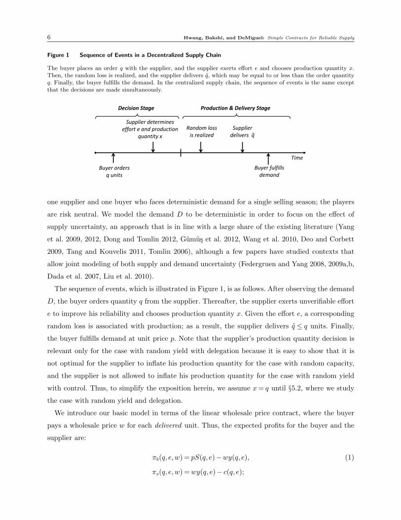
Figure 1 Sequence of Events in a Decentralized Supply Chain
The buyer places an order q with the supplier, and the supplier exerts effort e and chooses production quantity x.Then, the random loss is realized, and the supplier delivers q, which may be equal to or less than the order quantityq. Finally, the buyer fulfills the demand. In the centralized supply chain, the sequence of events is the same exceptthat the decisions are made simultaneously.
Buyer orders q units
Supplier determines effort e and production
quantity x
Random loss is realized
Supplier delivers 𝑞
Time
Decision Stage
Buyer fulfills demand
Production & Delivery Stage
one supplier and one buyer who faces deterministic demand for a single selling season; the players
are risk neutral. We model the demand D to be deterministic in order to focus on the effect of
supply uncertainty, an approach that is in line with a large share of the existing literature (Yang
et al. 2009, 2012, Dong and Tomlin 2012, Gumus et al. 2012, Wang et al. 2010, Deo and Corbett
2009, Tang and Kouvelis 2011, Tomlin 2006), although a few papers have studied contexts that
allow joint modeling of both supply and demand uncertainty (Federgruen and Yang 2008, 2009a,b,
Dada et al. 2007, Liu et al. 2010).
The sequence of events, which is illustrated in Figure 1, is as follows. After observing the demand
D, the buyer orders quantity q from the supplier. Thereafter, the supplier exerts unverifiable effort
e to improve his reliability and chooses production quantity x. Given the effort e, a corresponding
random loss is associated with production; as a result, the supplier delivers q ≤ q units. Finally,
the buyer fulfills demand at unit price p. Note that the supplier’s production quantity decision is
relevant only for the case with random yield with delegation because it is easy to show that it is
not optimal for the supplier to inflate his production quantity for the case with random capacity,
and the supplier is not allowed to inflate his production quantity for the case with random yield
with control. Thus, to simplify the exposition herein, we assume x= q until §5.2, where we study
the case with random yield and delegation.
We introduce our basic model in terms of the linear wholesale price contract, where the buyer
pays a wholesale price w for each delivered unit. Thus, the expected profits for the buyer and the
supplier are:
πb(q, e,w) = pS(q, e)−wy(q, e), (1)
πs(q, e,w) =wy(q, e)− c(q, e);
Hwang, Bakshi, and DeMiguel: Simple Contracts for Reliable Supply 7
where y(q, e), S(q, e), and c(q, e) are the expected values for the delivered quantity, sales, and cost,
respectively. In the centralized supply chain, the order quantity is the same as the production
quantity, and denoted by q. All decisions are made by a single entity, who maximizes the expected
supply-chain profit Π(q, e) = pS(q, e)− c(q, e). In the decentralized supply chain, the buyer acts
as a Stackelberg leader by deciding the order quantity. However, the buyer faces a moral hazard
problem because the supplier’s effort is not contractible. Our formulation is consistent with the
classical papers on moral hazard, e.g., Holmstrom (1979, p. 74-75), and Contract Theory textbooks,
e.g., Bolton and Dewatripont (2005, Section 1.3.2, and Chapter 4). As in the aforementioned
references, we assume the supplier’s objective function is common knowledge. Hence, when the
buyer (Stackelberg leader) decides her order quantity, she anticipates the supplier’s best response
to this order quantity, and decides accordingly. The buyer’s decision problem can therefore be
written as:
maxq
πb(q, e,w), (2)
s.t. e= argmaxe≥0
πs(q, e,w),
πs(q, e,w)≥ 0.
The first constraint ensures incentive compatibility for the supplier, i.e., the supplier chooses the
effort e that maximizes his expected profit. The second constraint ensures the supplier’s participa-
tion by providing the supplier with at least his reservation profit, which we normalize to zero.
A couple of comments are in order. First, note that we use the wholesale price w as a proxy
for relative bargaining power between buyer and supplier. In our treatment, a firm’s bargaining
power is proportional to the share of the entire supply-chain profit that it secures. Indeed, we have
verified that at equilibrium the supplier’s share of the overall supply chain profit is increasing in w,
while the buyer’s share is decreasing. Hence, we interpret a higher value of w as being consistent
with greater bargaining power for the supplier.
Second, rather than endogenizing the wholesale price w in problem (2), we treat it as exogenous.
In other words, the bargaining process by which w is determined is left unspecified. This is without
loss of generality for a given sequence of events; for instance, if we allow the buyer to choose w, she
will choose a value that maximizes her expected profit—a subset of the results obtained by exoge-
nously specifying w, and considering all possible values for w. Treating the contract parameters as
exogenous allows us to explore the entire spectrum of bargaining power: a standard approach in
the literature. The rationale behind this approach has been elaborated before in references such as
Cachon (2004, pp. 223-224).
Finally, to avoid trivial results and simplify exposition, we make the following assumption.
8 Hwang, Bakshi, and DeMiguel: Simple Contracts for Reliable Supply
Assumption 1. The following conditions hold:
(i) In the centralized supply chain, it is profitable to produce a strictly positive amount even when
the supplier does not exert any effort; that is, ∂Π(q, e)/∂q|q=0,e=0 > 0.
(ii) If the buyer is indifferent among order quantities Q ⊂ [0,D], then she chooses the largest
quantity q= supQ.
Assumption 1(i) ensures that the optimal production quantity in the centralized supply chain will
be strictly positive, and 1(ii) implies that the buyer will satisfy demand provided her profit is not
hurt, thus precluding Pareto suboptimal outcomes. We commence our analysis with the random
capacity scenario.
4. Random Capacity
With random capacity, we model disruptions that destroy part or all of the supplier’s capacity
(Ciarallo et al. 1994, Wang et al. 2010) and where the capacity loss is independent of the production
quantity. Examples include labor strike, machine breakdown, fire, and natural disaster.7 In §4.1,
we show how the basic model of §3 can be applied to the case of random capacity, state our
assumptions, and characterize the optimal decisions in the centralized supply chain. In §4.2, we
analyze the decentralized setup.
4.1. Model and Centralized Supply Chain
As mentioned in the previous section, it is easy to show that for the case with random capacity,
the supplier has no incentive to inflate his production quantity beyond the buyer’s order quantity;
therefore, without loss of generality we assume the production quantity x is equal to the order
quantity q. Consequently, the supplier delivers a random quantity q= min{q,K−ξ}, where q is the
order quantity, K is the supplier’s nominal capacity, and ξ is the random capacity loss. We assume
the random loss is ξ = fc(ψ,e), where ψ is a random variable that captures the underlying supply
risk and fc is a function that models the dependence of the random loss on the supplier’s effort e.
The density, and cumulative distribution function (CDF), for the random loss ξ conditional on the
effort e are denoted by g(ξ | e) and G(ξ | e), respectively. Finally, the expected delivered quantity
and expected sales are y(q, e) =Eξ[q] and S(q, e) =Eξ[min{q,D}], respectively.
We assume the supplier initiates production after the random loss is realized. Hence, the
expected cost is c(q, e) = cy(q, e) + v(e), where c is the unit production cost and v(e) is the cost of
effort to improve reliability. Additionally, we need the following technical assumption.
7 Note that we study random capacity losses as none of the disruptions mentioned above may result in an increase ofcapacity. Therefore the term random capacity loss would be more accurate than random capacity, but for consistencywith the existing literature, hereafter we use the term random capacity.
Hwang, Bakshi, and DeMiguel: Simple Contracts for Reliable Supply 9
Assumption 2. The following conditions hold:
(i) The random loss ξ has support [0, ac(e)], where both the CDF, G(ξ | e), and ac(e) are twice
continuously differentiable with finite derivatives in e≥ 0 and ξ ∈ [0, ac(e)].
(ii) Either of the following holds:
a) ac(e) =K, ∂G(ξ | e)/∂e > 0, ∂2G(ξ | e)/∂e2 < 0 for e≥ 0 and ξ ∈ (0,K).
b) ac(0) =K, a′c(e)< 0, ∂G(ξ | e)/∂e > 0, ∂2G(ξ | e)/∂e2 ≤ 0 for e≥ 0 and ξ ∈ (0, ac(e)].
(iii) The cost of effort is twice continuously differentiable and satisfies v(0) = 0 and v′(e) > 0,
v′′(e)≥ 0 for e > 0.
(iv) The effort level is strictly positive at equilibrium.
Part (ii) implies that the effort e mitigates the random loss ξ in the sense of first-order stochastic
dominance (FOSD) with decreasing returns to scale; and the supplier’s effort may (part a)), or
may not (part b)), reduce the range of the loss (ac(e)≤K). Part (iii) implies that the cost of the
supplier’s effort is convex and increasing. Part (iv) precludes the trivial case where the effort level
is zero, and allows us to simplify the exposition.
We find that if the order quantity is smaller than the demand (q ≤D), then so is the delivered
quantity q, and the buyer is able to sell everything; consequently the expected sales and delivered
quantities coincide (S(q, e) = y(q, e)). If the order quantity is larger than the demand (q >D), the
expected sales no longer depend on the order quantity q because the probability of receiving the
Dth unit is constant for q > D, and provided the buyer receives D units, she can fully satisfy
demand. Thus, the expected sales function S(q, e) has a kink at q=D. The technical properties of
S(q, e) and y(q, e) are summarized in Lemma 2 in Appendix A.1.
We now characterize the optimal order quantity and effort, (qo, eo), in the centralized supply
chain.
Proposition 1. Let Assumptions 1 and 2 hold. Then, in the centralized supply chain, there
exist unique optimal decisions (qo, eo), where the optimal order quantity qo is equal to demand D.
In the above result, the optimal effort eo satisfies the first-order condition (p− c)∂S(D,eo)/∂e=
v′(eo). The optimal order quantity qo is equal to the demand D because producing more does
not increase the expected sales. The only way to mitigate risk is for the supplier to exert effort.
Given that effort is unverifiable, we next address the efficiency of the wholesale price contract in a
decentralized supply chain.
4.2. Performance of the Wholesale Price Contract
We study the wholesale price contract and show that supply chain efficiency is generally increasing
in wholesale price, which we use as a proxy for the supplier’s bargaining power. Therefore, a
wholesale price contract may be the preferred mode of contracting for supply chains with sufficiently
powerful suppliers, even when a theoretically superior complex contract exists.
10 Hwang, Bakshi, and DeMiguel: Simple Contracts for Reliable Supply
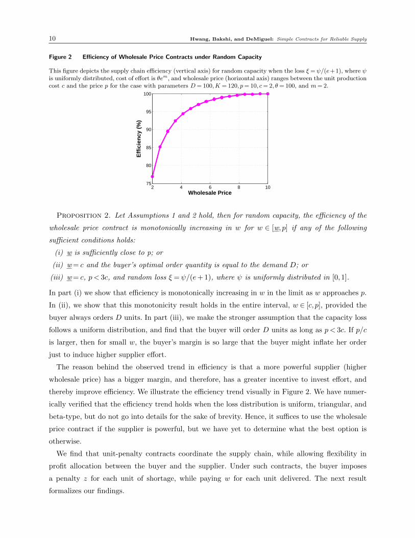
Figure 2 Efficiency of Wholesale Price Contracts under Random Capacity
This figure depicts the supply chain efficiency (vertical axis) for random capacity when the loss ξ =ψ/(e+1), where ψis uniformly distributed, cost of effort is θem, and wholesale price (horizontal axis) ranges between the unit productioncost c and the price p for the case with parameters D= 100,K = 120, p= 10, c= 2, θ= 100, and m= 2.
2 4 6 8 1075
80
85
90
95
100
Wholesale Price
Eff
icie
ncy
(%
)
Proposition 2. Let Assumptions 1 and 2 hold, then for random capacity, the efficiency of the
wholesale price contract is monotonically increasing in w for w ∈ [w, p] if any of the following
sufficient conditions holds:
(i) w is sufficiently close to p; or
(ii) w = c and the buyer’s optimal order quantity is equal to the demand D; or
(iii) w = c, p < 3c, and random loss ξ =ψ/(e+ 1), where ψ is uniformly distributed in [0,1].
In part (i) we show that efficiency is monotonically increasing in w in the limit as w approaches p.
In (ii), we show that this monotonicity result holds in the entire interval, w ∈ [c, p], provided the
buyer always orders D units. In part (iii), we make the stronger assumption that the capacity loss
follows a uniform distribution, and find that the buyer will order D units as long as p < 3c. If p/c
is larger, then for small w, the buyer’s margin is so large that the buyer might inflate her order
just to induce higher supplier effort.
The reason behind the observed trend in efficiency is that a more powerful supplier (higher
wholesale price) has a bigger margin, and therefore, has a greater incentive to invest effort, and
thereby improve efficiency. We illustrate the efficiency trend visually in Figure 2. We have numer-
ically verified that the efficiency trend holds when the loss distribution is uniform, triangular, and
beta-type, but do not go into details for the sake of brevity. Hence, it suffices to use the wholesale
price contract if the supplier is powerful, but we have yet to determine what the best option is
otherwise.
We find that unit-penalty contracts coordinate the supply chain, while allowing flexibility in
profit allocation between the buyer and the supplier. Under such contracts, the buyer imposes
a penalty z for each unit of shortage, while paying w for each unit delivered. The next result
formalizes our findings.
Hwang, Bakshi, and DeMiguel: Simple Contracts for Reliable Supply 11
Proposition 3. Let Assumptions 1 and 2 hold. Then, there exists χ > 0 such that the following
unit-penalty contracts coordinate the supply chain: w∗ = p−χ and z∗ = χ, where χ∈ [0, χ); and the
buyer’s expected profit is πb = χD.
By setting the unit-penalty z equal to her unit margin p− w, the buyer is able to transfer the
entire risk onto the supplier, which induces first-best effort. Flexible profit allocation is achieved
by varying χ, where the upper bound χ ensures that the supplier earns nonnegative profit and the
buyer does not inflate beyond D to take advantage of the high penalty fee. Thus, with random
capacity, bargaining power plays a key role: the wholesale price contract suffices when the supplier
is powerful, and a unit-penalty contract may be used to good effect otherwise. Would these insights
continue to hold if the nature of supply risk is altered to random yield instead, or does bargaining
power interact with supply risk in a qualitatively different manner? We address this question next.
5. Random Yield
With random yield, we model disruptions in which the random loss is stochastically proportional
to the production quantity, i.e., a larger production quantity increases the likelihood of obtaining
a larger amount of usable output (Federgruen and Yang 2008, 2009a,b, Tang and Kouvelis 2011).
It applies, for example, when manufacturers of semiconductor or biotech products face uncertain
yield in their manufacturing processes. The key distinguishing feature from random capacity is
that, in addition to effort, now inflating the production quantity (above demand) can be used as
an additional lever to mitigate supply risk.
Following the literature, we study two different cases that depend on the supplier’s decision
regarding production quantity. In §5.1 we examine the “control” scenario, in which the buyer
dictates the supplier’s production quantity decision, and in §5.2 we investigate the “delegation”
scenario, in which the supplier independently decides his production quantity, given the buyer’s
order. For each case, we show how the basic model of §3 can be applied, and discuss the performance
of the wholesale price contract.
5.1. Control Scenario
Federgruen and Yang (2009a) study a setting in which the buyer dictates the supplier’s production
quantity. They explain that this formulation is appropriate for contexts in which the supplier
cannot undertake full inspection of all produced units at his site.8 In such cases, since the buyer
will typically not accept a delivery in excess of her order quantity, the supplier will not inflate.
8 Full inspection at the supplier’s site is often impossible or impractical (e.g., Baiman et al. 2000, Balachandran andRadhakrishnan 2005), particularly when failures are mainly observed externally by the consumer (e.g., Kulp et al.2007), or when the testing technology is proprietary, and therefore the buyer deliberately limits the supplier’s abilityto detect failures due to intellectual property concerns (p23, Doucakis 2007).
12 Hwang, Bakshi, and DeMiguel: Simple Contracts for Reliable Supply
5.1.1. Model and Centralized Supply Chain. The supplier delivers a random quantity
q = (1− ξ)q, where q is the order quantity and ξ is the random proportional loss. To focus on the
effect of the random proportional loss, we assume here that the supplier has no capacity constraints.
We further assume that the random loss is ξ = fy(ψ,e), where ψ is a random variable that captures
the underlying supply risk and fy is a function that models the dependence of the random loss on
the supplier’s effort e. We denote the density and CDF of the random proportional loss as h(ξ | e)and H(ξ | e), respectively, and the expected random loss as E[ξ] = µey. The expected delivered
quantity and expected sales are y(q, e) =Eξ[q] and S(q, e) =Eξ[min{q,D}], respectively.
We assume the supplier incurs the production cost for all q units. This is reasonable as yield
and quality problems generally arise after all raw materials have been put into the production line.
Hence, the cost is c(q, e) = cq+ v(e). Additionally, we make the following assumption.
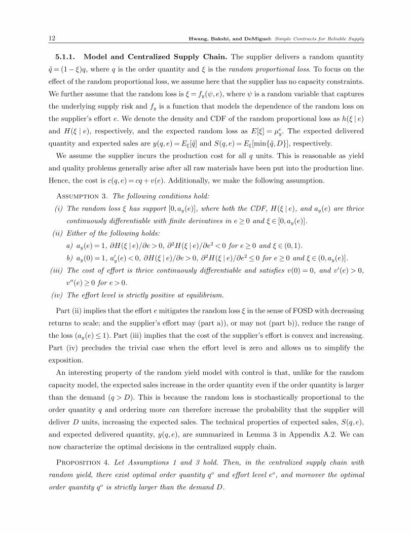
Assumption 3. The following conditions hold:
(i) The random loss ξ has support [0, ay(e)], where both the CDF, H(ξ | e), and ay(e) are thrice
continuously differentiable with finite derivatives in e≥ 0 and ξ ∈ [0, ay(e)].
(ii) Either of the following holds:
a) ay(e) = 1, ∂H(ξ | e)/∂e > 0, ∂2H(ξ | e)/∂e2 < 0 for e≥ 0 and ξ ∈ (0,1).
b) ay(0) = 1, a′y(e)< 0, ∂H(ξ | e)/∂e > 0, ∂2H(ξ | e)/∂e2 ≤ 0 for e≥ 0 and ξ ∈ (0, ay(e)].
(iii) The cost of effort is thrice continuously differentiable and satisfies v(0) = 0, and v′(e) > 0,
v′′(e)≥ 0 for e > 0.
(iv) The effort level is strictly positive at equilibrium.
Part (ii) implies that the effort emitigates the random loss ξ in the sense of FOSD with decreasing
returns to scale; and the supplier’s effort may (part a)), or may not (part b)), reduce the range of
the loss (ay(e)≤ 1). Part (iii) implies that the cost of the supplier’s effort is convex and increasing.
Part (iv) precludes the trivial case when the effort level is zero and allows us to simplify the
exposition.
An interesting property of the random yield model with control is that, unlike for the random
capacity model, the expected sales increase in the order quantity even if the order quantity is larger
than the demand (q > D). This is because the random loss is stochastically proportional to the
order quantity q and ordering more can therefore increase the probability that the supplier will
deliver D units, increasing the expected sales. The technical properties of expected sales, S(q, e),
and expected delivered quantity, y(q, e), are summarized in Lemma 3 in Appendix A.2. We can
now characterize the optimal decisions in the centralized supply chain.
Proposition 4. Let Assumptions 1 and 3 hold. Then, in the centralized supply chain with
random yield, there exist optimal order quantity qo and effort level eo, and moreover the optimal
order quantity qo is strictly larger than the demand D.
Hwang, Bakshi, and DeMiguel: Simple Contracts for Reliable Supply 13
The optimal decisions qo and eo satisfy the first-order necessary conditions: p ∂S(qo, eo)/∂q =
c and p ∂S(qo, eo)/∂e = v′(eo). Further, the optimal decisions differ qualitatively from those for
random capacity in Proposition 1; it is now optimal to order (or equivalently, produce) more than
the demand (qo > D). In other words, the decision maker increases the expected profit by not
only exerting effort but also ordering more. It is optimal to do so because it increases expected
sales, S(q, e), and the marginal benefit of such an increase at q = D, which is p∂S(D,e)/∂q, is
larger than the marginal cost c, a result that follows from Assumption 1(i). We investigate how,
in a decentralized setting, the need to coordinate the buyer’s order inflation, in addition to the
supplier’s effort, gives rise to different dynamics relative to random capacity.
5.1.2. Performance of the Wholesale Price Contract. Our main finding is that the
efficiency of the wholesale price contract generally decreases in the supplier’s bargaining power.
Therefore, the wholesale price contract is more likely to be the preferred mode of contracting when
the buyer is powerful. This result contrasts sharply with the result for random capacity, for which
the efficiency of the wholesale price contract increases in w. The reason is as follows. Similar to
random capacity, a higher wholesale price increases the supplier’s incentive to invest in reliability,
which has a positive impact on efficiency. However, increasing w also impacts efficiency negatively,
by reducing the buyer’s incentive to inflate her order quantity; the order quantity plays a dual role
by directly influencing proportional yield and indirectly generating incentives for the supplier to
invest effort, via a larger order size. Note that the supplier does not bear any overage cost, which
makes a larger order quantity more effective in inducing effort. Overall, due to the dual role played
by order quantity, the negative impact of higher wholesale price on inflation outweighs the positive
impact on effort, for the most part, thereby resulting in a decreasing trend in efficiency.
We now discuss the results that lead us to conclude that efficiency is generally decreasing in
wholesale price for random yield with control.
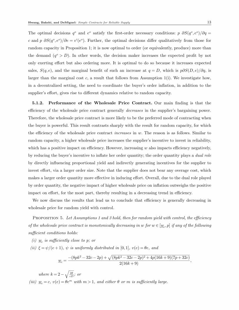
Proposition 5. Let Assumptions 1 and 3 hold, then for random yield with control, the efficiency
of the wholesale price contract is monotonically decreasing in w for w ∈ [wc, p] if any of the following
sufficient conditions holds:
(i) wc is sufficiently close to p; or
(ii) ξ =ψ/(e+ 1), ψ is uniformly distributed in [0,1], v(e) = θe, and
wc =−(8pk2− 32c− 2p) +
√(8pk2− 32c− 2p)2 + 4p(16k+ 9)(7p+ 32c)
2(16k+ 9),
where k= 2−√
2θcD
; or
(iii) wc = c, v(e) = θem with m> 1, and either θ or m is sufficiently large.
14 Hwang, Bakshi, and DeMiguel: Simple Contracts for Reliable Supply
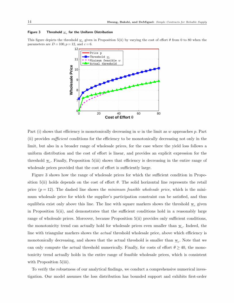
Figure 3 Threshold wc for the Uniform Distribution
This figure depicts the threshold wc given in Proposition 5(ii) by varying the cost of effort θ from 0 to 80 when theparameters are D= 100, p= 12, and c= 6.
0 20 40 60 806
7
8
9
10
11
12
Cost of Effort θ
Wh
ole
sale
Pri
ce
Price p
Threshold wc
Minimum feasible w
Actual threshold
Part (i) shows that efficiency is monotonically decreasing in w in the limit as w approaches p. Part
(ii) provides sufficient conditions for the efficiency to be monotonically decreasing not only in the
limit, but also in a broader range of wholesale prices, for the case where the yield loss follows a
uniform distribution and the cost of effort is linear, and provides an explicit expression for the
threshold wc. Finally, Proposition 5(iii) shows that efficiency is decreasing in the entire range of
wholesale prices provided that the cost of effort is sufficiently large.
Figure 3 shows how the range of wholesale prices for which the sufficient condition in Propo-
sition 5(ii) holds depends on the cost of effort θ. The solid horizontal line represents the retail
price (p = 12). The dashed line shows the minimum feasible wholesale price, which is the mini-
mum wholesale price for which the supplier’s participation constraint can be satisfied, and thus
equilibria exist only above this line. The line with square markers shows the threshold wc given
in Proposition 5(ii), and demonstrates that the sufficient conditions hold in a reasonably large
range of wholesale prices. Moreover, because Proposition 5(ii) provides only sufficient conditions,
the monotonicity trend can actually hold for wholesale prices even smaller than wc. Indeed, the
line with triangular markers shows the actual threshold wholesale price, above which efficiency is
monotonically decreasing, and shows that the actual threshold is smaller than wc. Note that we
can only compute the actual threshold numerically. Finally, for costs of effort θ ≥ 40, the mono-
tonicity trend actually holds in the entire range of feasible wholesale prices, which is consistent
with Proposition 5(iii).
To verify the robustness of our analytical findings, we conduct a comprehensive numerical inves-
tigation. Our model assumes the loss distribution has bounded support and exhibits first-order
Hwang, Bakshi, and DeMiguel: Simple Contracts for Reliable Supply 15
stochastic dominance (FOSD) as effort increases. We consider three loss distributions with bounded
support: uniform, triangular, and a beta-type distribution. The uniform distribution exhibits FOSD
as the support shrinks with greater effort. The triangular distribution exhibits FOSD as the mode
moves closer to zero with greater effort, while the support remains fixed. Finally, we consider a
beta-type distribution whose CDF has a closed-form expression9, and that exhibits FOSD with
fixed support as the mode gets closer to zero; see (Jones 2009). This beta-type distribution is
very flexible and encompasses a variety of bell shapes. To conserve space, we mainly emphasize
the results obtained with the uniform distribution, but our findings are robust to the use of the
triangular and beta-type distributions. The numerical setup for the uniform distribution case is as
follows.
NUMERICAL SETUP 1: (Random Yield) Let ξ = fy(ψ,e) = ψ/(e + 1), where ψ is uniformly
distributed in [0,1]. The cost is c(q, e) = cq+ θem, where c, θ > 0 and m≥ 1.
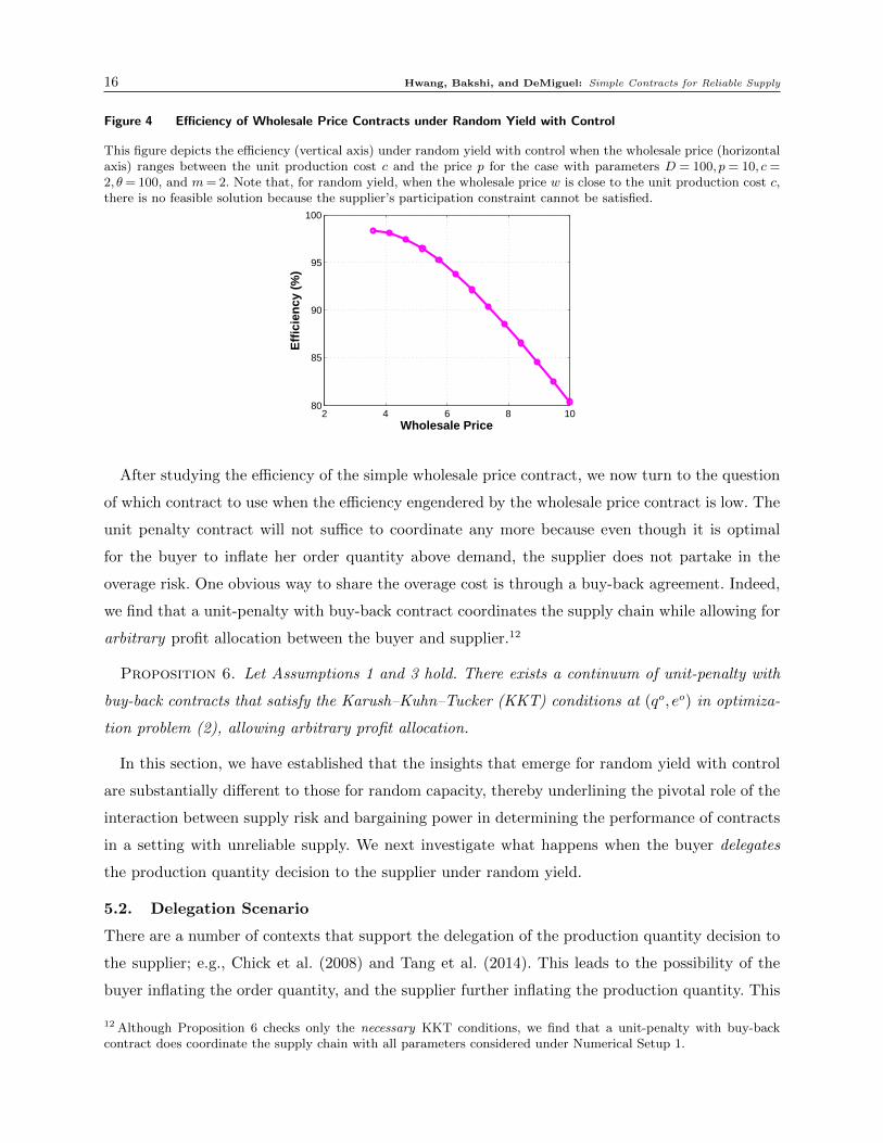
Figure 4 depicts the efficiency as a function of wholesale price for the same set of parameters
as for Figure 2. We observe a very robust decreasing trend in efficiency. Specifically, the efficiency
is fairly high (∼ 98%) when the buyer is powerful but is relatively low (∼ 80%) when the supplier
is powerful. We then repeated our experiment with different parameter combinations; we chose
seven values each for c, θ, and m in the following ranges: c = [0.1,5], θ = [1,100],m = [1,5]. We
therefore performed our analysis with 73=343 different combinations of parameters. We found that
the efficiency was monotonically decreasing in the entire range of wholesale prices in 84.3% of cases.
The remaining 15.7% of cases exhibited a slight increase in efficiency (typically less than 0.1%)
for small w only, but the general decreasing trend was preserved elsewhere.10 We explored the
triangular distribution with the same combinations of parameters and found complete monotonicity
in efficiency in 100% of cases. For the beta-type distribution, we conducted the numerical analysis
with a narrower range of parameters to ensure feasibility, and again found monotonicity in efficiency
in 97.8% of cases.11 The remaining 2.2% exhibited a slight increase for small w, but again the
general decreasing trend was preserved.
9 Specifically, the CDF is H(ξ | e) = 1− (1− ξa)e, where a is a parameter and e is the effort level.
10 The reason why the decreasing monotonicity trend may not hold when w is sufficiently close to c can be tracedback to the fact that both effort and quantity exhibit diminishing marginal impact (returns to scale) on expectedsales, and therefore on efficiency; the relevant derivatives can be found in Table 2 in Appendix B. This means that asw increases, the marginal increase in efficiency due to additional effort is higher when w is close to c, and the baselineeffort is small; and correspondingly the marginal loss in efficiency due to the decrease in order quantity is relativelylower. Hence, if the monotonicity trend in efficiency were to be violated at all, it would happen when w is close to c,which is consistent with our result in Proposition 5.
11 The beta-type distribution generally results in higher yield losses compared to the other distributions, and theselosses are increasing in a. Therefore, we use a narrower range of parameters to ensure feasible solutions. Specifically,we chose five values each for a,c,θ, and m in the following ranges: a= [1,3], c ∈ [0.1, c], θ ∈ [1, θ],m= [1,5], where i)c = 3, θ = 100 for a = 1 and 1.5; ii) c = 2, θ = 50 for a = 2 and 2.5; and iii) c = 1, θ = 50 for a = 3. This results in54 = 625 cases.
16 Hwang, Bakshi, and DeMiguel: Simple Contracts for Reliable Supply
Figure 4 Efficiency of Wholesale Price Contracts under Random Yield with Control
This figure depicts the efficiency (vertical axis) under random yield with control when the wholesale price (horizontalaxis) ranges between the unit production cost c and the price p for the case with parameters D = 100, p = 10, c =2, θ= 100, and m= 2. Note that, for random yield, when the wholesale price w is close to the unit production cost c,there is no feasible solution because the supplier’s participation constraint cannot be satisfied.
2 4 6 8 1080
85
90
95
100
Wholesale Price
Eff
icie
ncy
(%
)
After studying the efficiency of the simple wholesale price contract, we now turn to the question
of which contract to use when the efficiency engendered by the wholesale price contract is low. The
unit penalty contract will not suffice to coordinate any more because even though it is optimal
for the buyer to inflate her order quantity above demand, the supplier does not partake in the
overage risk. One obvious way to share the overage cost is through a buy-back agreement. Indeed,
we find that a unit-penalty with buy-back contract coordinates the supply chain while allowing for
arbitrary profit allocation between the buyer and supplier.12
Proposition 6. Let Assumptions 1 and 3 hold. There exists a continuum of unit-penalty with
buy-back contracts that satisfy the Karush–Kuhn–Tucker (KKT) conditions at (qo, eo) in optimiza-
tion problem (2), allowing arbitrary profit allocation.
In this section, we have established that the insights that emerge for random yield with control
are substantially different to those for random capacity, thereby underlining the pivotal role of the
interaction between supply risk and bargaining power in determining the performance of contracts
in a setting with unreliable supply. We next investigate what happens when the buyer delegates
the production quantity decision to the supplier under random yield.
5.2. Delegation Scenario
There are a number of contexts that support the delegation of the production quantity decision to
the supplier; e.g., Chick et al. (2008) and Tang et al. (2014). This leads to the possibility of the
buyer inflating the order quantity, and the supplier further inflating the production quantity. This
12 Although Proposition 6 checks only the necessary KKT conditions, we find that a unit-penalty with buy-backcontract does coordinate the supply chain with all parameters considered under Numerical Setup 1.
Hwang, Bakshi, and DeMiguel: Simple Contracts for Reliable Supply 17
aspect introduces an additional source of inefficiency into the supply chain: the supplier potentially
inflates the production quantity, even if the buyer has already padded her order quantity to buffer
against yield losses. These buffers may accumulate and exacerbate inefficiency. We now examine
whether this is indeed the case.
5.2.1. Model and Centralized Supply Chain. The model is similar to that of the control
scenario in §5.1 except that the supplier determines his own production quantity x. Therefore, we
present only those parts of the model that are different from the control scenario. The supplier
delivers a random quantity q= min{q, (1− ξ)x}, where q is the order quantity, x is the production
quantity, and ξ is the random proportional loss as defined in §5.1. The expected delivered quantity
is represented as y(q,x, e) = Eξ[q] and the expected sales, S(q,x, e) = Eξ[min{q,D}]. The cost is
c(x, e) = cx+ v(e). For tractability, we also make the following assumption.
Assumption 4. The expected delivered quantity y(q,x, e) is jointly concave in q and e, and also
in x and e in the feasible region in problem (2).
While it is difficult to establish the above property in general, we have verified analytically that it
is satisfied by the uniform distribution, i.e., when random proportional loss ξ = ψ/(e+ 1), where
ψ is uniformly distributed in [0,1].
Unlike the control scenario, if the order quantity is larger than the demand (q >D), the expected
sales become constant, as in the random capacity model. This is because as long as q ≥D, the
probability of receiving D units depends only on the production quantity x and the effort e.
Therefore, ordering more than D does not directly increase the expected sales, and S(q,x, e) has a
kink at q=D. Note, however, that higher q does give the supplier an incentive to choose higher x
and e, and can thereby indirectly increase expected sales. The properties of S(q,x, e) and y(q,x, e)
are summarized in Lemma 4 in Appendix A.3.
In the centralized supply chain, the order quantity is redundant, and the decision maker chooses
only the production quantity x and the effort e. Therefore, the optimal decisions in the centralized
supply chain are the same as for the control case discussed in §5.1 except that we replace the order
quantity q with the production quantity x in Proposition 4 and refer to the optimal production
quantity as xo. We examine the decentralized setup next.
5.2.2. Performance of the Wholesale Price Contract. We discover that the efficiency
associated with the wholesale price contract exhibits a V -shaped pattern, as we increase the whole-
sale price (supplier’s bargaining power); this contrasts with both the random capacity model and
the random yield with control scenario. Therefore, we argue that with the delegation of the pro-
duction quantity decision, if either party possesses the bulk of the bargaining power, then the
18 Hwang, Bakshi, and DeMiguel: Simple Contracts for Reliable Supply
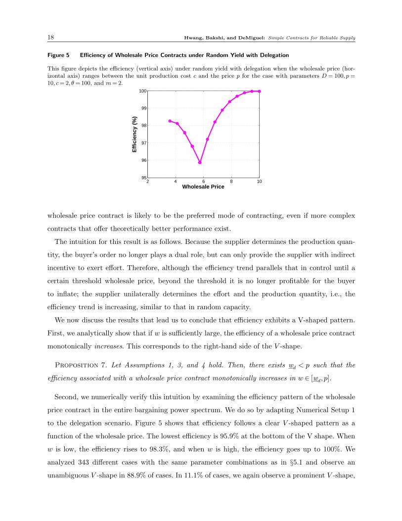
Figure 5 Efficiency of Wholesale Price Contracts under Random Yield with Delegation
This figure depicts the efficiency (vertical axis) under random yield with delegation when the wholesale price (hor-izontal axis) ranges between the unit production cost c and the price p for the case with parameters D = 100, p =10, c= 2, θ= 100, and m= 2.
2 4 6 8 1095
96
97
98
99
100
Wholesale Price
Eff
icie
ncy
(%
)
wholesale price contract is likely to be the preferred mode of contracting, even if more complex
contracts that offer theoretically better performance exist.
The intuition for this result is as follows. Because the supplier determines the production quan-
tity, the buyer’s order no longer plays a dual role, but can only provide the supplier with indirect
incentive to exert effort. Therefore, although the efficiency trend parallels that in control until a
certain threshold wholesale price, beyond the threshold it is no longer profitable for the buyer
to inflate; the supplier unilaterally determines the effort and the production quantity, i.e., the
efficiency trend is increasing, similar to that in random capacity.
We now discuss the results that lead us to conclude that efficiency exhibits a V-shaped pattern.
First, we analytically show that if w is sufficiently large, the efficiency of a wholesale price contract
monotonically increases. This corresponds to the right-hand side of the V -shape.
Proposition 7. Let Assumptions 1, 3, and 4 hold. Then, there exists wd < p such that the
efficiency associated with a wholesale price contract monotonically increases in w ∈ [wd, p].
Second, we numerically verify this intuition by examining the efficiency pattern of the wholesale
price contract in the entire bargaining power spectrum. We do so by adapting Numerical Setup 1
to the delegation scenario. Figure 5 shows that efficiency follows a clear V -shaped pattern as a
function of the wholesale price. The lowest efficiency is 95.9% at the bottom of the V shape. When
w is low, the efficiency rises to 98.3%, and when w is high, the efficiency goes up to 100%. We
analyzed 343 different cases with the same parameter combinations as in §5.1 and observe an
unambiguous V -shape in 88.9% of cases. In 11.1% of cases, we again observe a prominent V -shape,
Hwang, Bakshi, and DeMiguel: Simple Contracts for Reliable Supply 19
but with a slight increase in efficiency (typically less than 0.1%) when w is very low (on the left
extreme of the bargaining power spectrum), followed by the expected V -shaped pattern.13
Our results above suggest that when thinking about using incentives to improve supply relia-
bility in a decentralized supply chain, one must consider whether the buyer controls or delegates
the production quantity decision, in addition to bargaining power and the nature of supply risk.
Interestingly, for the delegation scenario, we find that as we increase the margin (and therefore
payoff) of the supplier (the agent undertaking unverifiable action), the trend in efficiency is neither
monotonically increasing (as with random capacity) nor monotonically decreasing (as with random
yield with control), but is instead V -shaped.
To consolidate this insight, there is still one remaining loose end: which contract coordinates in
the delegation scenario? We address this next.
Proposition 8. Let Assumptions 1, 3, and 4 hold. There exists χ > 0 such that the following
unit-penalty contracts coordinate the supply chain: w∗ = p− χ, z∗ = χ, where 0 ≤ χ ≤ χ; and the
buyer’s expected profit is πb = χD.
Interestingly, we find that a unit-penalty contract coordinates the supply chain with flexible profit
allocation, even though there exists an additional dimension of moral hazard (production quantity)
in comparison to the control scenario, which requires the more complex unit-penalty with buy-back
contract for coordination. The intuition is that if the penalty fee is set equal to the margin (and is
not too large), then the buyer does not inflate the order, because for each unit of demand she can
make her margin through either a sale or the penalty imposed on the supplier. Then, the supplier
faces exactly the same trade-offs as the centralized decision maker and thus chooses the first-best
effort and production quantity.
While the business context may impose the procurement process design in the form of either
the control or the delegation scenario, it could also be a choice for the decision maker—the central
planner or the player with the dominant bargaining power. In such a case, a natural question would
be, which of the two—control or delegation—results in greater efficiency, and how do the fortunes
of the buyer and the supplier compare in the two scenarios. We address this next.
13 With the triangular distribution, we observe an unambiguous V -shape in 85.1% of cases. Also, in 1.4% of cases,we find a prominent V -shape but with a slight increase in efficiency at the left extreme of the V . In 13.5% of cases,the efficiency was just increasing; but these are exceptional cases when the unit production cost c is so high thatfeasible solutions therefore exist only when the wholesale price w is at least as large as 90% of the retail price. For thebeta-type distribution, we observe an unambiguous V-shape in 97.1% of cases. In 1.9% of cases, we find a prominentV-shape but with a slight increase in efficiency at the left extreme of V, and in 1% of cases, the efficiency was justincreasing.
20 Hwang, Bakshi, and DeMiguel: Simple Contracts for Reliable Supply
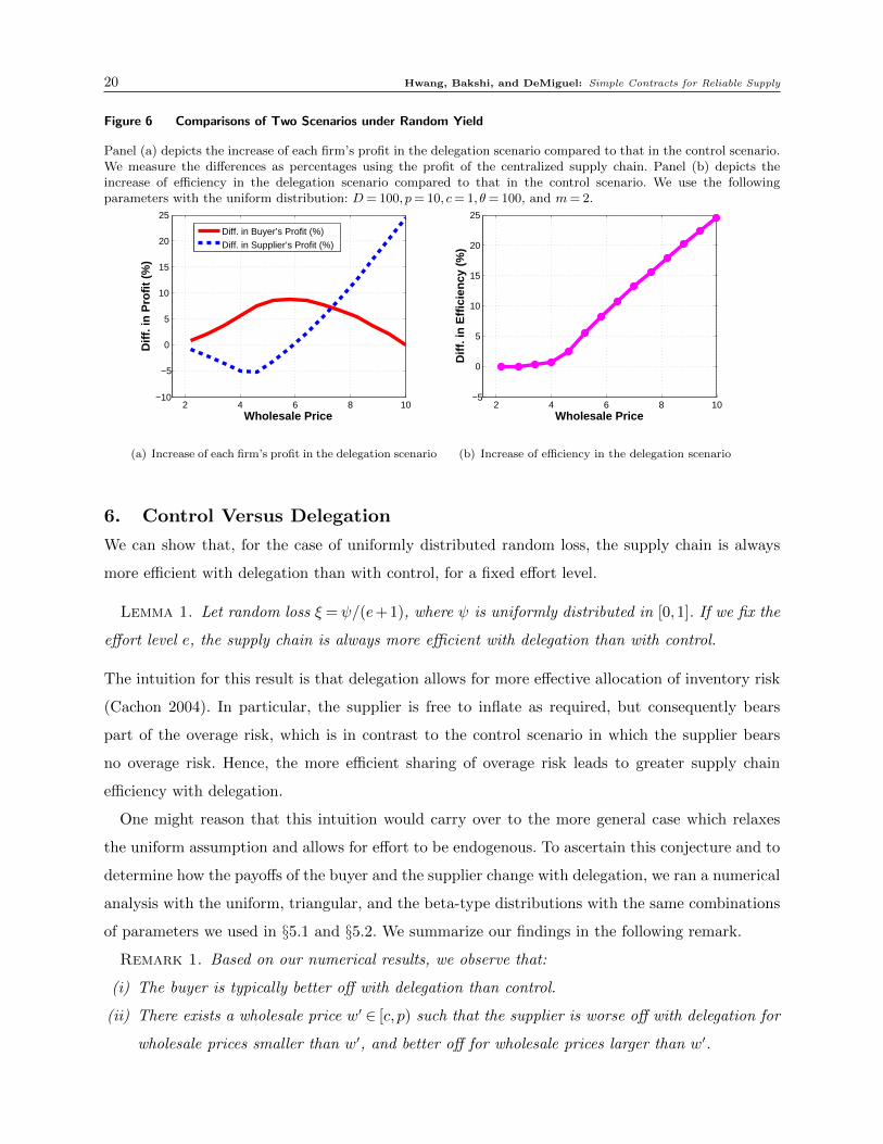
Figure 6 Comparisons of Two Scenarios under Random Yield
Panel (a) depicts the increase of each firm’s profit in the delegation scenario compared to that in the control scenario.We measure the differences as percentages using the profit of the centralized supply chain. Panel (b) depicts theincrease of efficiency in the delegation scenario compared to that in the control scenario. We use the followingparameters with the uniform distribution: D= 100, p= 10, c= 1, θ= 100, and m= 2.
2 4 6 8 10−10
−5
0
5
10
15
20
25
Wholesale Price
Dif
f. in
Pro
fit
(%)
Diff. in Buyer’s Profit (%)Diff. in Supplier’s Profit (%)
(a) Increase of each firm’s profit in the delegation scenario
2 4 6 8 10−5
0
5
10
15
20
25
Wholesale Price
Dif
f. in
Eff
icie
ncy
(%
)(b) Increase of efficiency in the delegation scenario
6. Control Versus Delegation
We can show that, for the case of uniformly distributed random loss, the supply chain is always
more efficient with delegation than with control, for a fixed effort level.
Lemma 1. Let random loss ξ =ψ/(e+1), where ψ is uniformly distributed in [0,1]. If we fix the
effort level e, the supply chain is always more efficient with delegation than with control.
The intuition for this result is that delegation allows for more effective allocation of inventory risk
(Cachon 2004). In particular, the supplier is free to inflate as required, but consequently bears
part of the overage risk, which is in contrast to the control scenario in which the supplier bears
no overage risk. Hence, the more efficient sharing of overage risk leads to greater supply chain
efficiency with delegation.
One might reason that this intuition would carry over to the more general case which relaxes
the uniform assumption and allows for effort to be endogenous. To ascertain this conjecture and to
determine how the payoffs of the buyer and the supplier change with delegation, we ran a numerical
analysis with the uniform, triangular, and the beta-type distributions with the same combinations
of parameters we used in §5.1 and §5.2. We summarize our findings in the following remark.
Remark 1. Based on our numerical results, we observe that:
(i) The buyer is typically better off with delegation than control.
(ii) There exists a wholesale price w′ ∈ [c, p) such that the supplier is worse off with delegation for
wholesale prices smaller than w′, and better off for wholesale prices larger than w′.
Hwang, Bakshi, and DeMiguel: Simple Contracts for Reliable Supply 21
(iii) There exists a wholesale price w′′ ∈ [c, p) such that the efficiency is lower with delegation for
wholesale prices smaller than w′′, and higher for wholesale prices larger than w′′. Moreover,
w′′ ≤w′.
The reason for the above findings lies essentially in the intuition provided by Lemma 1. Specif-
ically, the explanation for part (i) is that in the control scenario, the supplier is precluded from
sharing any overage cost because he cannot inflate the production quantity, while in the delegation
scenario, the supplier is free to inflate as required. This additional flexibility for the supplier is
deceptive because the buyer anticipates the supplier’s best response and adjusts her order quan-
tity to induce optimal (for her) sharing of the overage risk: the supplier now bears the overage
cost for units produced in excess of the buyer’s order quantity. Thus, by virtue of reallocating the
inventory risk in the supply chain, the buyer finds that she is better off delegating the production
decision to the supplier. The above also forms the basis for the observation in part (ii). Although
one might expect that the supplier would always be better off in the delegation scenario owing
to the additional flexibility in decision making (the supplier chooses effort as well as production
quantity), an offsetting influence is introduced as he now shares the overage risk. The latter effect
dominates when the buyer is powerful (low wholesale price). Finally, combining the insights from
parts (i) and (ii) provides the basis for understanding the result in part (iii), because the efficiency
is determined by the sum of both firms’ profits. It is worth noting that the loss in efficiency, when
it occurs, is minimal (generally less than 1.5%), while the gain in efficiency can be great (between
10% and 30%). We visually illustrate the findings of Remark 1 in Figure 6.
Thus, it seems that, in a setting with unreliable supply (random yield), delegation of the produc-
tion decision to the supplier can actually mitigate the incentive alignment challenge for the buyer
and improve supply-chain efficiency.
7. Conclusions
We have investigated how the linear wholesale price contract can be used to generate efficient
outcomes in a decentralized supply chain, when supply reliability can be improved, but the
supplier’s effort is unverifiable. We characterize how the performance the wholesale-price contract
depends on the interplay between the nature of supply risk, the balance of bargaining power, and
whether the buyer controls or delegates the production quantity decision. Below, we summarize
our two major findings and their managerial implications.
Moral Hazard and the Use of Appropriate Contracts. Heuristic reasoning suggests that as
an agent undertaking unverifiable action is awarded a bigger share of the overall margin, he will
have greater incentive to invest in the action; this would mitigate the incentive alignment challenge
22 Hwang, Bakshi, and DeMiguel: Simple Contracts for Reliable Supply
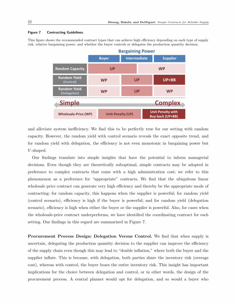
Figure 7 Contracting Guidelines.
This figure shows the recommended contract types that can achieve high efficiency depending on each type of supplyrisk, relative bargaining power, and whether the buyer controls or delegates the production quantity decision.
Random Capacity
Buyer
WP UP
Supplier
Random Yield (Delegation) WP WP UP
Intermediate
Bargaining Power
Complex Simple
Wholesale-Price (WP) Unit-Penalty (UP) Unit-Penalty with Buy-back (UP+BB)
Random Yield (Control) WP UP UP+BB
and alleviate system inefficiency. We find this to be perfectly true for our setting with random
capacity. However, the random yield with control scenario reveals the exact opposite trend, and
for random yield with delegation, the efficiency is not even monotonic in bargaining power but
V -shaped.
Our findings translate into simple insights that have the potential to inform managerial
decisions. Even though they are theoretically suboptimal, simple contracts may be adopted in
preference to complex contracts that come with a high administration cost; we refer to this
phenomenon as a preference for “appropriate” contracts. We find that the ubiquitous linear
wholesale price contract can generate very high efficiency and thereby be the appropriate mode of
contracting: for random capacity, this happens when the supplier is powerful; for random yield
(control scenario), efficiency is high if the buyer is powerful; and for random yield (delegation
scenario), efficiency is high when either the buyer or the supplier is powerful. Also, for cases when
the wholesale-price contract underperforms, we have identified the coordinating contract for each
setting. Our findings in this regard are summarized in Figure 7.
Procurement Process Design: Delegation Versus Control. We find that when supply is
uncertain, delegating the production quantity decision to the supplier can improve the efficiency
of the supply chain even though this may lead to “double inflation,” where both the buyer and the
supplier inflate. This is because, with delegation, both parties share the inventory risk (overage
cost), whereas with control, the buyer bears the entire inventory risk. This insight has important
implications for the choice between delegation and control, or in other words, the design of the
procurement process. A central planner would opt for delegation, and so would a buyer who
Hwang, Bakshi, and DeMiguel: Simple Contracts for Reliable Supply 23
enjoys the requisite bargaining power to impose her choice. For instance, a powerful buyer such as
Hewlett-Packard, can potentially impose the production quantity decision on the supplier (contract
manufacturer) because it procures input materials on behalf of the supplier (Supply Chain Brain
2006, Amaral et al. 2006), and can therefore preclude supplier inflation by limiting the inputs
supplied. Our results suggest that such a strategy would be counter-productive for the buyer.
Finally, we note that our one-shot model is limited in its ability to handle multi-period con-
siderations such as reputational effects and relational contracts (incentives in the form of promise
of future business, or threat of termination of relationship); further, it does not account for the
simultaneous presence of capacity and yield uncertainty. Extending our work in these directions
could be fruitful avenues for future research.
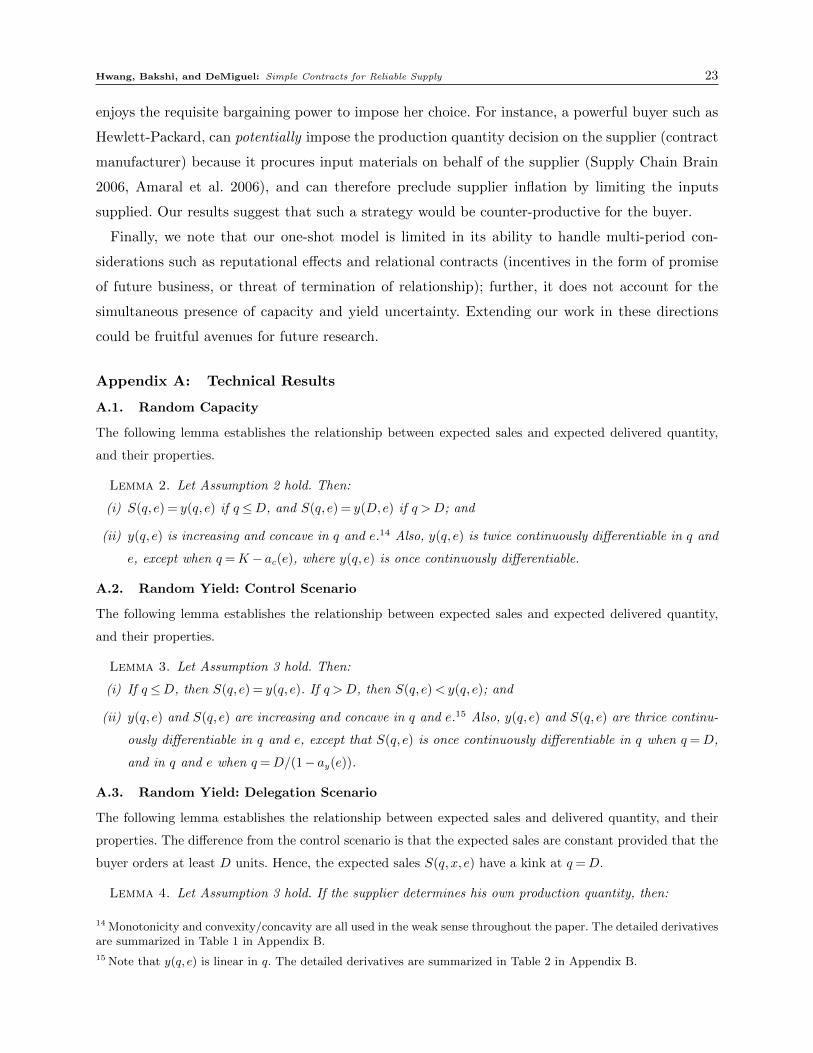
Appendix A: Technical Results
A.1. Random Capacity
The following lemma establishes the relationship between expected sales and expected delivered quantity,
and their properties.
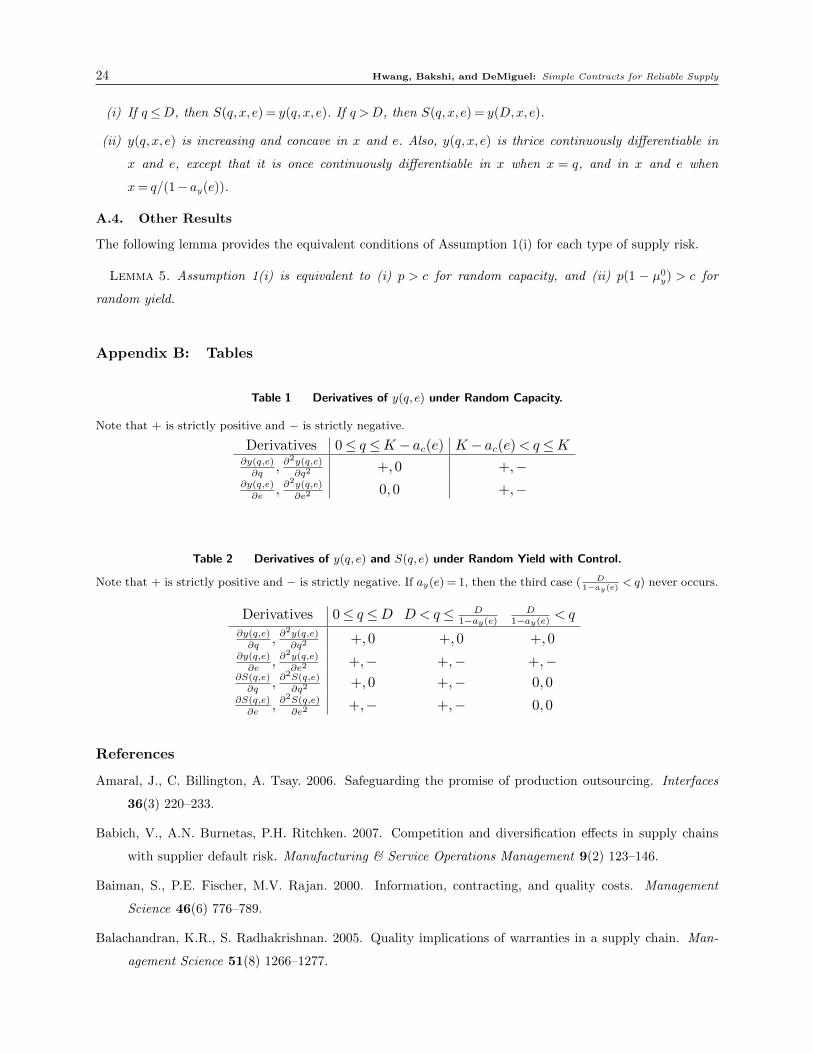
Lemma 2. Let Assumption 2 hold. Then:
(i) S(q, e) = y(q, e) if q≤D, and S(q, e) = y(D,e) if q >D; and
(ii) y(q, e) is increasing and concave in q and e.14 Also, y(q, e) is twice continuously differentiable in q and
e, except when q=K − ac(e), where y(q, e) is once continuously differentiable.
A.2. Random Yield: Control Scenario
The following lemma establishes the relationship between expected sales and expected delivered quantity,
and their properties.
Lemma 3. Let Assumption 3 hold. Then:
(i) If q≤D, then S(q, e) = y(q, e). If q >D, then S(q, e)< y(q, e); and
(ii) y(q, e) and S(q, e) are increasing and concave in q and e.15 Also, y(q, e) and S(q, e) are thrice continu-
ously differentiable in q and e, except that S(q, e) is once continuously differentiable in q when q =D,
and in q and e when q=D/(1− ay(e)).
A.3. Random Yield: Delegation Scenario
The following lemma establishes the relationship between expected sales and delivered quantity, and their
properties. The difference from the control scenario is that the expected sales are constant provided that the
buyer orders at least D units. Hence, the expected sales S(q,x, e) have a kink at q=D.
Lemma 4. Let Assumption 3 hold. If the supplier determines his own production quantity, then:
14 Monotonicity and convexity/concavity are all used in the weak sense throughout the paper. The detailed derivativesare summarized in Table 1 in Appendix B.
15 Note that y(q, e) is linear in q. The detailed derivatives are summarized in Table 2 in Appendix B.
24 Hwang, Bakshi, and DeMiguel: Simple Contracts for Reliable Supply
(i) If q≤D, then S(q,x, e) = y(q,x, e). If q >D, then S(q,x, e) = y(D,x, e).
(ii) y(q,x, e) is increasing and concave in x and e. Also, y(q,x, e) is thrice continuously differentiable in
x and e, except that it is once continuously differentiable in x when x = q, and in x and e when
x= q/(1− ay(e)).
A.4. Other Results
The following lemma provides the equivalent conditions of Assumption 1(i) for each type of supply risk.
Lemma 5. Assumption 1(i) is equivalent to (i) p > c for random capacity, and (ii) p(1 − µ0y) > c for
random yield.
Appendix B: Tables
Table 1 Derivatives of y(q, e) under Random Capacity.
Note that + is strictly positive and − is strictly negative.
Derivatives 0≤ q≤K − ac(e) K − ac(e)< q≤K∂y(q,e)
∂q, ∂
2y(q,e)
∂q2+,0 +,−
∂y(q,e)
∂e, ∂
2y(q,e)
∂e20,0 +,−
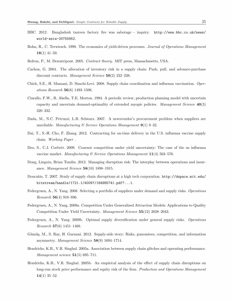
Table 2 Derivatives of y(q, e) and S(q, e) under Random Yield with Control.
Note that + is strictly positive and − is strictly negative. If ay(e) = 1, then the third case ( D1−ay(e)
< q) never occurs.
Derivatives 0≤ q≤D D< q≤ D1−ay(e)
D1−ay(e) < q
∂y(q,e)
∂q, ∂
2y(q,e)
∂q2+,0 +,0 +,0
∂y(q,e)
∂e, ∂
2y(q,e)
∂e2+,− +,− +,−
∂S(q,e)
∂q, ∂
2S(q,e)
∂q2+,0 +,− 0,0
∂S(q,e)
∂e, ∂
2S(q,e)
∂e2+,− +,− 0,0
References
Amaral, J., C. Billington, A. Tsay. 2006. Safeguarding the promise of production outsourcing. Interfaces
36(3) 220–233.
Babich, V., A.N. Burnetas, P.H. Ritchken. 2007. Competition and diversification effects in supply chains
with supplier default risk. Manufacturing & Service Operations Management 9(2) 123–146.
Baiman, S., P.E. Fischer, M.V. Rajan. 2000. Information, contracting, and quality costs. Management
Science 46(6) 776–789.
Balachandran, K.R., S. Radhakrishnan. 2005. Quality implications of warranties in a supply chain. Man-
agement Science 51(8) 1266–1277.
Hwang, Bakshi, and DeMiguel: Simple Contracts for Reliable Supply 25
BBC. 2012. Bangladesh tazreen factory fire was sabotage - inquiry. http://www.bbc.co.uk/news/
world-asia-20755952.
Bohn, R., C. Terwiesch. 1999. The economics of yield-driven processes. Journal of Operations Management
18(1) 41–59.
Bolton, P., M. Dewatripont. 2005. Contract theory . MIT press, Massachusetts, USA.
Cachon, G. 2004. The allocation of inventory risk in a supply chain: Push, pull, and advance-purchase
discount contracts. Management Science 50(2) 222–238.
Chick, S.E., H. Mamani, D. Simchi-Levi. 2008. Supply chain coordination and influenza vaccination. Oper-
ations Research 56(6) 1493–1506.
Ciarallo, F.W., R. Akella, T.E. Morton. 1994. A periodic review, production planning model with uncertain
capacity and uncertain demand-optimality of extended myopic policies. Management Science 40(3)
320–332.
Dada, M., N.C. Petruzzi, L.B. Schwarz. 2007. A newsvendor’s procurement problem when suppliers are
unreliable. Manufacturing & Service Operations Management 9(1) 9–32.
Dai, T., S.-H. Cho, F. Zhang. 2012. Contracting for on-time delivery in the U.S. influenza vaccine supply
chain. Working Paper .
Deo, S., C.J. Corbett. 2009. Cournot competition under yield uncertainty: The case of the us influenza
vaccine market. Manufacturing & Service Operations Management 11(4) 563–576.
Dong, Lingxiu, Brian Tomlin. 2012. Managing disruption risk: The interplay between operations and insur-
ance. Management Science 58(10) 1898–1915.
Doucakis, T. 2007. Study of supply chain disruptions at a high tech corporation. http://dspace.mit.edu/
bitstream/handle/1721.1/40097/184985741.pdf?...1.
Federgruen, A., N. Yang. 2008. Selecting a portfolio of suppliers under demand and supply risks. Operations
Research 56(4) 916–936.
Federgruen, A., N. Yang. 2009a. Competition Under Generalized Attraction Models: Applications to Quality
Competition Under Yield Uncertainty. Management Science 55(12) 2028–2043.
Federgruen, A., N. Yang. 2009b. Optimal supply diversification under general supply risks. Operations
Research 57(6) 1451–1468.
Gumus, M., S. Ray, H. Gurnani. 2012. Supply-side story: Risks, guarantees, competition, and information
asymmetry. Management Science 58(9) 1694–1714.
Hendricks, K.B., V.R. Singhal. 2005a. Association between supply chain glitches and operating performance.
Management science 51(5) 695–711.
Hendricks, K.B., V.R. Singhal. 2005b. An empirical analysis of the effect of supply chain disruptions on
long-run stock price performance and equity risk of the firm. Production and Operations Management
14(1) 35–52.
26 Hwang, Bakshi, and DeMiguel: Simple Contracts for Reliable Supply
Holmstrom, B. 1979. Moral hazard and observability. The Bell Journal of Economics 74–91.
Jones, MC. 2009. Kumaraswamys distribution: A beta-type distribution with some tractability advantages.
Statistical Methodology 6(1) 70–81.
Kalkancı, B., K-Y. Chen, F. Erhun. 2011. Contract complexity and performance under asymmetric demand
information: An experimental evaluation. Management science 57(4) 689–704.
Kalkancı, B., K-Y. Chen, F. Erhun. 2014. Complexity as a contract design factor: A human-to-human
experimental study. Production and Operations Management 23(2) 269–284.
Kulp, S., N. DeHoratius, Z. Kanji. 2007. Vendor compliance at geoffrey ryans (a). Harvard Business Review
9–108–022.
Lariviere, M., E. Porteus. 2001. Selling to the newsvendor: An analysis of price-only contracts. Manufacturing
& Service Operations Management 3(4) 293–305.
Lexology. 2010. Implications of recent labor unrest for mncs operating or investing in china. http://www.
lexology.com/library/detail.aspx?g=f31127fe-281f-4773-9e32-a37407977212.
Liu, S., K.C. So, F. Zhang. 2010. Effect of supply reliability in a retail setting with joint marketing and
inventory decisions. Manufacturing & Service Operations Management 12(1) 19–32.
Luenberger, D.G., Y. Ye. 2008. Linear and Nonlinear Programming . Springer.
Mas-Colell, A., M.D. Whinston, J.R. Green. 1995. Microeconomic theory . Oxford university press New York.
New York Times. 2009. Disaster recovery. http://www.nytimes.com/2009/09/10/business/
smallbusiness/10disaster.html?_r=0.
New York Times. 2011. Disaster in japan batters suppliers. http://www.nytimes.com/2011/03/15/
business/global/15supply.html.
Perakis, G., G. Roels. 2007. The price of anarchy in supply chains: Quantifying the efficiency of price-only
contracts. Management Science 53(8) 1249–1268.
Pitchford, R. 1998. Moral hazard and limited liability: The real effects of contract bargaining. Economics
Letters 61(2) 251–259.
Rowell, D., L. Connelly. 2012. A history of the term moral hazard. Journal of Risk and Insurance 79(4)
1051–1075.
Schwartz, A., J. Watson. 2004. The law and economics of costly contracting. The Journal of Law, Economics,
and Organization 20(1) 2–31.
Snow, D., S. Wheelwright, A. Wagonfeld. 2006. Genentech – capacity planning. Harvard Business Review
9–606–052.
Supply Chain Brain. 2006. Hp shows how to outsource production while keep-
ing control over suppliers. http://www.supplychainbrain.com/content/
research-analysis/supply-chain-innovation-awards/single-article-page/article/
hp-shows-how-to-outsource-production-while-keeping-control-over-suppliers-1/.
Hwang, Bakshi, and DeMiguel: Simple Contracts for Reliable Supply 27
Tang, S., H. Gurnani, D. Gupta. 2014. Managing disruptions in decentralized supply chains with endogenous
supply process reliability. Production and Operations Management forthcoming.
Tang, S.Y., P. Kouvelis. 2011. Supplier diversification strategies in the presence of yield uncertainty and
buyer competition. Manufacturing & Service Operations Management 13(4) 439–451.
The Wall Street Journal. 2010. Firms boost pay for chinese. http://online.wsj.com/news/articles/
SB10001424052748703685404575306633125903208.
The Wall Street Journal. 2012. Companies test backup plans, and learn some lessons. http://online.wsj.
com/article/SB10001424052970204840504578089083861617790.html.
Tomlin, B. 2006. On the value of mitigation and contingency strategies for managing supply chain disruption
risks. Management Science 52(5) 639–657.
Tomlin, B. 2009. Impact of supply learning when suppliers are unreliable. Manufacturing & Service Opera-
tions Management 11(2) 192–209.
Tomlin, B., Y. Wang. 2005. On the value of mix flexibility and dual sourcing in unreliable newsvendor
networks. Manufacturing & Service Operations Management 7(1) 37–57.
Wang, Y., W. Gilland, B. Tomlin. 2010. Mitigating supply risk: dual sourcing or process improvement?
Manufacturing & Service Operations Management 12(3) 489–510.
Yang, Z.B., G. Aydın, V. Babich, D.R. Beil. 2009. Supply disruptions, asymmetric information, and a backup
production option. Management Science 55(2) 192–209.
Yang, Z.B., G. Aydın, V. Babich, D.R. Beil. 2012. Using a dual-sourcing option in the presence of asym-
metric information about supplier reliability: Competition vs. diversification. Manufacturing & Service
Operations Management 14(2) 202–217.
28 Hwang, Bakshi, and DeMiguel: Simple Contracts for Reliable Supply
Appendix C: Proofs of All Results
We first provide proofs for the four lemmas in Appendix A, and then provide proofs for all propositions and
lemmas in the same order as they appear in the paper, because we use the results in Appendix A extensively
in the proofs.
Proof of Lemma 2(i) The expected sales is S(q, e) =Eξ[min{min{q,K − ξ},D}]. If q ≤D, then S(q, e) =
Eξ[min{q,K − ξ}] = y(q, e), by definition. If q >D, then S(q, e) =Eξ[min{D,K − ξ}] = y(D,e). �
Proof of Lemma 2(ii) We show the property with respect to q in Part (1) and with respect to e in Part
(2). The monotonicity and concavity properties are used in the weak sense, and the detailed derivatives are
summarized in Table 1.
(1) Property of y(q, e) in q: Recall that ac(e) is the maximum random loss. For any given e ≥ 0, let
q(e) =K − ac(e), which is the capacity that is never affected by the random loss. We consider the following
two cases, 0≤ q≤ q(e) and q(e)≤ q≤K, and check the continuity and differentiability at q= q(e).
First, if 0≤ q≤ q(e), then q≤K−ac(e), and the order is never affected by the random loss. Thus, y(q, e) =
Eξ[min{q,K − ξ}] = q. Also, ∂y(q, e)/∂q = 1 > 0 and ∂2y(q, e)/∂q2 = 0. Thus, y(q, e) is twice continuously
differentiable, increasing, and concave in q.
Second, if q(e)≤ q≤K, then q≥K−ac(e), and a fraction of the order quantity is affected by the random
loss. Hence
y(q, e) =Eξ[min{q,K − ξ}] =
∫ K−q
0
qg(ξ | e)dξ+
∫ ac(e)
K−q(K − ξ)g(ξ | e)dξ = (K − ac(e)) +
∫ ac(e)
K−qG(ξ | e)dξ,
where the last equality is obtained from integration by parts. y(q, e) is twice continuously differentiable in
q by Leibniz integral rule, because G(ξ | e) and ac(e) are twice continuously differentiable in q (which are
zeros), and so is K − q. Therefore,
∂y(q, e)
∂q= 0 ·G(ac(e) | e) +G(K − q | e) +
∫ ac(e)
K−q
∂G(ξ | e)∂q
dξ =G(K − q | e)> 0.
Also, ∂2y(q, e)/∂q2 = −g(K − q | e) < 0 because K − q is in the support [0, ac(e)]. Hence, y(q, e) is twice
continuously differentiable, increasing, and concave in q.
Last, we check the differentiability at q = q(e). We have y(q(e), e) = Eξ[min{q(e),K − ξ}] = q(e). Also,
limq→q(e)− y(q, e) = limq→q(e)− q= q(e), and
limq→q(e)+
y(q, e) = limq→q(e)+
[(K − ac(e)) +
∫ ac(e)
K−qG(ξ | e)dξ
]=K − ac(e) = q(e).
In addition, limq→q(e)− ∂y(q, e)/∂q = limq→q(e)− 1 = 1, and limq→q(e)+ ∂y(q, e)/∂q = limq→q(e)+ G(K − q | e) =
G(ac(e) | e) = 1. Thus, y(q, e) is once continuously differentiable at q= q(e).
(2) Property of y(q, e) in e: Recall that ac(e) is the maximum random loss, and K−ac(e) is the capacity
that is not affected by the random loss. Assumption 2 states that either i) ac(e) = K for all e ≥ 0 or ii)
ac(0) =K and a′c(e)< 0 for all e≥ 0. Hence, for a given q, there may exist e′ > 0 such that q =K − ac(e′).We assume such e′ exists, and consider two cases, 0 ≤ e < e′ and e′ ≤ e, and check the differentiability at
e= e′. (The case when such e′ does not exist trivially follows from this general case.)
Hwang, Bakshi, and DeMiguel: Simple Contracts for Reliable Supply 29
First, if 0≤ e < e′, then q >K − ac(e), and we know y(q, e) = (K − ac(e)) +∫ ac(e)
K−q G(ξ | e)dξ from Part (1)
of this proof. y(q, e) is continuously differentiable in e by Leibniz integral rule, because G(ξ | e) and ac(e) are
continuously differentiable in e by Assumption 2, and so is K − q. Thus,
∂y(q, e)
∂e=−a′c(e) + a′c(e)G(ac(e) | e) +
∫ ac(e)
K−q
∂G(ξ | e)∂e
dξ =
∫ ac(e)
K−q
∂G(ξ | e)∂e
dξ,
because G(ac(e) | e) = 1. Since ∂G(ξ | e)/∂e > 0 for all ξ ∈ (0, ac(e)) by Assumption 2, and ac(e)>K− q, it is
obvious that ∂y(q, e)/∂e > 0. Again, ∂y(q, e)/∂e is continuously differentiable in e because ∂G(ξ | e)/∂e and
ac(e) are continuously differentiable by Assumption 2, and thus
∂2y(q, e)
∂e2= a′c(e)
∂G(ac(e) | e)∂e
+
∫ ac(e)
K−q
∂2G(ξ | e)∂e2
dξ.
By Assumption 2, either i) a′c(e) = 0, ∂2G(ξ | e)/∂e2 < 0 for e ≥ 0 and ξ ∈ (0,K), or ii) a′c(e) < 0, ∂G(ξ |
e)/∂e > 0, ∂2G(ξ | e)/∂e2 ≤ 0 for all e ≥ 0 and ξ ∈ (0, ac(e)]. Either way, we have that ∂2y(q, e)/∂e2 < 0.
Hence, y(q, e) is twice continuously differentiable, increasing, and strictly concave in e.
Second, if e′ ≤ e, then q ≤K − ac(e). In this case, y(q, e) = q, and ∂y(q, e)/∂e= ∂2y(q, e)/∂e2 = 0. Hence,
y(q, e) is twice continuously differentiable, increasing, and concave in e.
Last, we check continuity and differentiability at e= e′. We have y(q, e′) = q, lime→e′+ y(q, e) = lime→e′+ q=
q and
lime→e′−
y(q, e) = lime→e′−
(K − ac(e)) +
∫ ac(e)
K−qG(ξ | e)dξ = q,
since ac(e′) =K − q. Also, lime→e′+ ∂y(q, e)/∂e= lime→e′+ 0 = 0, and
lime→e′−
∂y(q, e)
∂e= lime→e′−
∫ ac(e)
K−q
∂G(ξ | e)∂e
dξ = 0,
because lime→e′− ac(e) =K− q and ∂G(ξ | e)/∂e is finite by Assumption 2. Thus, y(q, e) is once continuously
differentiable at e= e′. �
Proof of Lemma 3(i) We look at three cases. First, if q ≤ D, then (1 − ξ)q ≤ D, because 0 ≤ ξ ≤ 1.
Therefore, S(q, e) =Eξ[min{(1− ξ)q,D}=Eξ[(1− ξ)q] = y(q, e), by definition.
Second, if q >D and (1−ay(e))q≥D, then the demand can be always met even with the maximum random
loss. (Recall that ξ = ay(e) is the maximum random loss.) Hence, S(q, e) =Eξ[min{(1−ξ)q,D}] =Eξ[D] =D.
Thus, y(q, e) =Eξ[(1− ξ)q] = (1−µey)q > (1− ay(e))q≥D= S(q, e), since µey <ay(e).
Third, if q >D and (1−ay(e))q <D, then a fraction of the demand may not be met. Specifically, min{(1−
ξ)q,D}=D if 0≤ ξ ≤ 1−D/q and min{(1− ξ)q,D}= (1− ξ)q if 1−D/q < ξ ≤ ay(e). Therefore,
S(q, e) =Eξ[min{(1− ξ)q,D}] =
∫ 1−Dq
0
D ·h(ξ | e)dξ+
∫ ay(e)
1−Dq
(1− ξ)q ·h(ξ | e)dξ.
Note that y(q, e) =Eξ[(1−ξ)q] =∫ ay(e)
0(1−ξ)q ·h(ξ | e)dξ. Hence, y(q, e)−S(q, e) =
∫ 1−D/q0
((1−ξ)q−D)h(ξ |
e)dξ > 0, since (1− ξ)q >D when ξ ∈ (0,1−D/q).
30 Hwang, Bakshi, and DeMiguel: Simple Contracts for Reliable Supply
For further uses in the rest of the proofs, we simplify S(q, e). Using integration by parts, we have
S(q, e) =DH
(1− D
q| e)
+ (1− ay(e))q−D+
∫ ay(e)
1−Dq
q ·H(ξ | e)dξ
= (1− ay(e))q+
∫ ay(e)
1−Dq
q ·H(ξ | e)dξ.
�
Proof of Lemma 3(ii) Since we are showing the properties of y(q, e) and S(q, e) with respect to both q
and e, we divide the proof into four parts: (1) y(q, e) with q, (2) S(q, e) with q, (3) y(q, e) with e, and (4)
S(q, e) with e. Note that the monotonicity and concavity properties are used in the weak sense.
(1) Property of y(q, e) in q: For any e≥ 0, y(q, e) = (1− µey)q, and hence y(q, e) is thrice continuously
differentiable in q. Also, ∂y(q, e)/∂q = (1−µey)> 0, because 0≤ µey < 1, and ∂2y(q, e)/∂q2 = 0. Thus, y(q, e)
is increasing and concave in q.
(2) Property of S(q, e) in q: We consider three cases in which we have different functional forms: (a)
q <D, (b) D< q <D/(1−ay(e)), and (c) D/(1−ay(e))< q. Also, we check once differentiability at the two
boundaries between three cases. If ay(e) = 1, the third case never happens, but the result trivially follows
from this more general case. Thus, we assume ay(e) 6= 1.
First, if q < D, then S(q, e) = y(q, e) from part (i) of this Lemma. Thus, S(q, e) is thrice continuously
differentiable, increasing, and concave in q.
Second, if D< q <D/(1−ay(e)), then S(q, e) = (1−ay(e))q+∫ ay(e)
1−D/q qH(ξ | e)dξ from the proof of part (i)
of this Lemma. S(q, e) is thrice continuously differentiable in q by Leibniz integral rule, because H(ξ | e) and
ac(e) are thrice continuously differentiable in q (note that both are independent of q), and so is (1−D/q).
Thus,
∂S(q, e)
∂q= (1− ay(e))−
D
qH
(1− D
q| e)
+
∫ ay(e)
1−Dq
H(ξ | e)dξ
=
∫ ay(e)
1−Dq
[H(ξ | e)−H
(1− D
q| e)]
dξ+ (1− ay(e))(
1−H(
1− D
q| e))
.
The first integral term is strictly positive, because H(ξ | e)−H(1−D/q | e) is strictly positive when 1−D/q <
ξ ≤ ay(e). Also, the second term is strictly positive, because 1−D/q < ay(e) and thus H(1−D/q | e)< 1,
and we assumed ay(e)< 1. Therefore, ∂S(q, e)/∂q > 0. Again, using Leibniz integral rule,
∂2S(q, e)
∂q2=D
q2H
(1− D
q| e)− D2
q3h
(1− D
q| e)− D
q2H
(1− D
q| e)
=−D2
q3h
(1− D
q| e).
Therefore, ∂2S(q, e)/∂q2 < 0, because h(1−D/q | e)> 0 since 1−D/q lies in the support [0, ay(e)]. Hence,
S(q, e) is thrice continuously differentiable, increasing, and strictly concave in q.
Third, if D/(1 − ay(e)) < q, then S(q, e) = D from the proof of Lemma 3(i). This is obviously thrice
continuously differentiable in q, increasing (∂S(q, e)/∂q= 0), and concave (∂2S(q, e)/∂q2 = 0).
Now, we show S(q, e) is once continuously differentiable in q at the two boundaries. First, we look at
q=D. We have that S(D,e) = (1−µey)D, limq→D− S(q, e) = limq→D−(1−µey)q= (1−µey)D, and
Hwang, Bakshi, and DeMiguel: Simple Contracts for Reliable Supply 31
limq→D+
S(q, e) = limq→D+
[(1− ay(e))q+
∫ ay(e)
1−Dq
qH(ξ | e)dξ
]= (1− ay(e))D+
∫ ay(e)
0
D ·H(ξ | e)dξ
= (1− ay(e))D+
(ay(e)−
∫ ay(e)
0
ξh(ξ | e)dξ
)D=
(1−
∫ ay(e)
0
ξh(ξ | e)dξ
)D= (1−µey)D.
Therefore, S(q, e) is continuous in q at q=D. Also, we observe that limq→D− ∂S(q, e)/∂q= limq→D−(1−µey) =
(1−µey), and
limq→D+
∂S(q, e)
∂q= limq→D+
[∫ ay(e)
1−Dq
[H(ξ | e)−H
(1− D
q| e)]
dξ+ (1− ay(e))(
1−H(
1− D
q| e))]
=
∫ ay(e)
0
H(ξ | e)dξ+ (1− ay(e)) = ay(e)−∫ ay(e)
0
ξh(ξ | e)dξ+ (1− ay(e)) = (1−µey),
using integration by parts. Therefore, S(q, e) is once continuously differentiable in q when q=D.
Second, we consider q=D/(1−ay(e)). Let q(e) =D/(1−ay(e)). Then, S(q(e), e) =D, limq→q(e)+ S(q, e) =
D, and
limq→q(e)−
S(q, e) = limq→q(e)−
[(1− ay(e))q+
∫ ay(e)
1−Dq
qH(ξ | e)dξ
]=D.
Hence, S(q, e) is continuous in q at q=D/(1− ay(e)). Also, limq→q(e)+ ∂S(q, e)/∂q= limq→q(e)+ 0 = 0, and
limq→q(e)−
∂S(q, e)
∂q= limq→q(e)−
[(1− ay(e))−
D
qH
(1− D
q| e)
+
∫ ay(e)
1−D/qH(ξ | e)dξ
]
= (1− ay(e))− (1− ay(e))H(ay(e) | e) +
∫ ay(e)
ay(e)
H(ξ | e)dξ = 0,
since H(ay(e) | e) = 1. Therefore, S(q, e) is once continuously differentiable in q when q=D/(1− ay(e)).
(3) Property of y(q, e) in e: Note that y(q, e) = (1 − µey)q = (1 −∫ ay(e)
0ξh(ξ | e)dξ)q = (1 − ay(e) +∫ ay(e)
0H(ξ | e)dξ)q by integration by parts. We find y(q, e) is continuously differentiable in e by Leibniz
integral rule, because H(ξ | e) and ay(e) are continuously differentiable in e by Assumption 3. Therefore,
∂y(q, e)
∂e=
[−a′y(e) + a′y(e)H(ay(e) | e) +
∫ ay(e)
0
∂H(ξ | e)∂e
dξ
]q= q
∫ ay(e)
0
∂H(ξ | e)∂e
dξ,
because H(ay(e) | e) = 1. Since ∂H(ξ | e)/∂e > 0 when ξ ∈ (0, ay(e)) by Assumption 3, we get ∂y(q, e)/∂e > 0
if q > 0, and ∂y(q, e)/∂e= 0 if q = 0. In addition, ∂y(q, e)/∂e is twice more continuously differentiable in e,
because ∂H(ξ | e)/∂e and ay(e) are twice continuously differentiable in e by Assumption 3. Thus,
∂2y(q, e)
∂e2= q
[a′y(e)
∂H(ay(e) | e)∂e
+
∫ ay(e)
0
∂2H(ξ | e)∂e2
dξ
].
Assumption 3 states that either i) a′y(e) = 0 and ∂2H(ξ | e)/∂e2 < 0 for e≥ 0 and ξ ∈ (0,1), or ii) a′y(e)< 0,
∂H(ξ | e)/∂e > 0, and ∂2H(ξ | e)/∂e2 ≤ 0 for e≥ 0 and ξ ∈ (0, ay(e)]. Either way, we have that ∂2y(q, e)/∂e2 <
0. Therefore, y(q, e) is thrice continuously differentiable, increasing, and strictly concave in e.
(4) Property of S(q, e) in e: Following a similar structure to that of part (2), we consider three cases:
i) q ≤D, ii) D< q <D/(1− ay(e)), and iii) D/(1− ay(e))< q. However, unlike part (2), the only boundary
we need to check is the one between cases ii) and iii), because the boundary between cases i) and ii) are not
32 Hwang, Bakshi, and DeMiguel: Simple Contracts for Reliable Supply
determined by e. As in part (2), if ay(e) = 1, then the third case never occurs, but this is subsumed in the
more general three case scenario, so we assume ay(e) 6= 1.
First, if q≤D, then S(q, e) = y(q, e) by part (i) of this Lemma. Therefore, the result follows from part (3).
Second, if D< q <D/(1−ay(e)), then S(q, e) = (1−ay(e))q+∫ ay(e)
1−D/q qH(ξ | e)dξ from the proof of Lemma
3(i). We find S(q, e) is continuously differentiable in e by Leibniz integral rule, because H(ξ | e) and ay(e)
are continuously differentiable in e by Assumption 3, and so is 1−D/q. Therefore,
∂S(q, e)
∂e=−a′y(e)q+
[a′y(e)H(ay(e) | e) +
∫ ay(e)
1−Dq
∂H(ξ | e)∂e
dξ
]q= q
∫ ay(e)
1−Dq
∂H(ξ | e)∂e
dξ,
because H(ay(e) | e) = 1. Note that ∂H(ξ | e)/∂e > 0 when ξ ∈ (0, ay(e)) by Assumption 3. Thus,
∂S(q, e)/∂e > 0 if q > 0 and ∂S(q, e)/∂e = 0 if q = 0. In addition, ∂S(q, e)/∂e is twice more continuously
differentiable in e, because ∂H(ξ | e)/∂e and ay(e) are twice continuously differentiable in e by Assumption 3.
Thus,
∂2S(q, e)
∂e2= q
[a′y(e)
∂H(ay(e) | e)∂e
+
∫ ay(e)
1−Dq
∂2H(ξ | e)∂e2
dξ
].
Assumption 3 states that either i) a′y(e) = 0 and ∂2H(ξ | e)/∂e2 < 0 for e≥ 0 and ξ ∈ (0,1), or ii) a′y(e)< 0,
∂H(ξ | e)/∂e > 0, and ∂2H(ξ | e)/∂e2 ≤ 0 for e≥ 0 and ξ ∈ (0, ay(e)]. Either way, we have that ∂2S(q, e)/∂e2 <
0. Hence, S(q, e) is thrice continuously differentiable, increasing, and strictly concave in e.
Third, if D/(1−ay(e))< q, then S(q, e) =D, and hence ∂S(q, e)/∂e= ∂2S(q, e)/∂e2 = 0. Therefore, S(q, e)
is thrice continuously differentiable, increasing, and concave in e.
Now, we check once differentiability at e such that q = D/(1− ay(e)). Assume there exists e′ such that
q =D/(1− ay(e′)). If e < e′, then q < D/(1− ay(e)), and in the neighborhood of e′ we fall into the second
case above, and thus S(q, e) = (1− ay(e))q +∫ ay(e)
1−D/q qH(ξ | e)dξ. If e≥ e′, then q ≥D/(1− ay(e)), which is
the third case above. Hence, S(q, e) =D. At e= e′, we have S(q, e′) =D, lime→e′+ S(q, e) = lime→e′+ D=D,
and
lime→e′−
S(q, e) = lime→e′−
[(1− ay(e))q+
∫ ay(e)
1−D/qqH(ξ | e)dξ
]=D.
In addition, lime→e′+ ∂S(q, e)/∂e= lime→e′+ 0 = 0, and
lime→e′−
∂S(q, e)
∂e= lime→e′−
q
(∫ ay(e)
1−Dq
∂H(ξ | e)∂e
dξ
)= 0.
Therefore, S(q, e) is once continuously differentiable at e= e′. �
Proof of Lemma 4(i) If q ≤D, then S(q,x, e) =Eξ[min{q,D}] =Eξ[min{q, (1− ξ)x,D}] =Eξ[min{q, (1−ξ)x}] = y(q,x, e). If q≥D, then S(q,x, e) =Eξ[min{q, (1− ξ)x,D}] =Eξ[min{(1− ξ)x,D}] = y(D,x, e). �
Proof of Lemma 4(ii) y(q,x, e) =Eξ[min{(1− ξ)x, q}] is equivalent to S(x, e) =Eξ[min{(1− ξ)x,D}] if we
set q=D. Therefore, we can obtain the stated properties of y(q,x, e) from S(x, e) in Lemma 3. �
Proof of Lemma 5(i) For random capacity, Π(q, e) = pS(q, e)− (cy(q, e) + v(e)). Note that, when q ≤D,
S(q, e) = y(q, e) by Lemma 2 and ∂y(q, e)/∂q=G(K−q | e) by the proof of Lemma 2. Therefore, when q≤D,
Hwang, Bakshi, and DeMiguel: Simple Contracts for Reliable Supply 33
∂Π(q,0)/∂q= (p− c)∂y(q,0)/∂q= (p− c)G(K− q | 0). Thus, ∂Π(0,0)/∂q= p− c, and hence Assumption 1(i)
is equivalent to p > c. �
Proof of Lemma 5(ii) For random yield, Π(q, e) = pS(q, e) − (cq + v(e)). By Lemma 3, when q ≤ D,
S(q, e) = y(q, e) = (1− µey)q. Therefore, when q ≤D, ∂Π(0,0)/∂q = p(1− µ0y)− c. Hence, Assumption 1(i) is
equivalent to p(1−µ0y)> c. �
Proof of Proposition 1 The proof is organized in two steps. In Step 1, we show that the optimal order
(production) quantity is qo =D regardless of effort e. In Step 2, we show that eo is uniquely obtained by the
first-order condition.
Step 1: Optimal order quantity. The expected profit is Π(q, e) = pS(q, e)− (cy(q, e) + v(e)). We consider
two cases: 1) q >D and 2) q <D. If q >D, then S(q, e) = y(D,e) by Lemma 2, and hence Π(q, e) = py(D,e)−
(cy(q, e) + v(e))< py(D,e)− (cy(D,e) + v(e)) = Π(D,e), since ∂y(q, e)/∂q > 0 by Lemma 2 and Table 1. If
q <D, then S(q, e) = y(q, e) by Lemma 2, and hence Π(q, e) = (p− c)y(q, e)− v(e)< (p− c)y(D,e)− v(e) =
Π(D,e), since ∂y(q, e)/∂q > 0, and p > c by Lemma 5. Therefore, the solution is qo =D regardless of e.
Step 2: Optimal effort. With qo =D, we have Π(D,e) = (p− c)y(D,e)− v(e), since S(D,e) = y(D,e) by
Lemma 2. Π(D,e) is strictly concave in e, because y(D,e) is strictly concave in e by Lemma 2 and Table 1
and v(e) is convex by Assumption 2. Thus, the optimal effort eo can be uniquely obtained by the the first-
order condition: ∂Π(D,e)/∂e= (p− c)∂S(D,e)/∂e−v′(e) = 0. (Note that we focus only on interior solutions
by Assumption 2.) �
Proof of Proposition 2(i) This proof is organized in three steps. Let e(q) be the supplier’s best response
function. In Step 1, we show that, if w> c, then e(q) is once continuously differentiable, has a finite derivative,
and de(q)/dq > 0. In Step 2, we show that the buyer always orders at least D units, and if de(q)/dq is finite,
then there exists w < p such that for all w ∈ [w,p], the optimal order quantity is q∗ =D. Finally, in Step 3,
we show that, if q=D is fixed, then the efficiency is strictly increasing in w.
Step 1: The supplier’s best response function e(q). The supplier’s expected profit is πs(q, e) = (w−
c)y(q, e)−v(e), and this is once continuously differentiable in e by Lemma 2 and Assumption 2. The optimal
effort is uniquely obtained by the first-order condition, ∂πs(q, e)/∂e= 0, because πs(q, e) is strictly concave
in e, since y(q, e) is strictly concave in e by Lemma 2 and Table 1 and v(e) is convex by Assumption 2. (Note
that we focus only on interior solutions by Assumption 2.)
Note that πs(q, e) is twice continuously differentiable in the neighborhood of the optimal solution. It
is because πs(q, e) is twice continuously differentiable in both q and e if q 6= K − ac(e) by Lemma 2 and
Assumption 2, and the optimal effort indeed satisfies q 6= K − ac(e). If q = K − ac(e), then y(q, e) = q,
∂y(q, e)/∂e = 0, and thus the first-order condition cannot be satisfied. Therefore, by the implicit function
theorem, e(q) is once continuously differentiable (Luenberger and Ye 2008), and we have
de(q)
dq=−∂
2πs(q, e)
∂e∂q
(∂2πs(q, e)
∂e2
)−1
=(w− c) ∂
2y(q,e)
∂e∂q
v′′(e)− (w− c) ∂2y(q,e)∂e2
. (3)
34 Hwang, Bakshi, and DeMiguel: Simple Contracts for Reliable Supply
First, ∂y(q, e)/∂q = G(K − q | e) from the proof of Lemma 2, and thus ∂2y(q, e)/∂e∂q = ∂G(K − q | e)/∂e
is strictly positive and finite by Assumption 2. Second, if w > c, then v′′(e)− (w − c) ∂2y(q,e)
∂e2> 0, because
v′′(e)≥ 0 by Assumption 2 and ∂2y(q, e)/∂e2 < 0 by Lemma 2 and Table 1. Hence if w> c, then de(q)/dq is
strictly positive and finite.
Step 2: Optimal order quantity. First, we show that we can ignore the supplier’s participation constraint
in problem (2). Second, we show that the buyer’s expected profit πb(q) is always increasing in q when q≤D,
and there exists w< p such that if w≥w, πb(q) is decreasing in q when q≥D. Then, we can conclude that,
if w≥w, the optimal order quantity is D.
First, the supplier’s participation constraint is always satisfied because of the following reason. The sup-
plier’s expected profit πs(q, e) = (w− c)y(q, e)− v(e) is strictly concave in e since y(q, e) is strictly concave
in e by Lemma 2 and Table 1, and v(e) is convex in e by Assumption 2. In addition, if w ∈ [c, p], then
πs(q,0) = (w− c)y(q,0)− v(0) = (w− c)y(q,0)≥ 0, because v(0) = 0 by Assumption 2. Thus, the supplier’s
first-order condition that generates a strictly positive effort (by Assumption 2) always produces a set of
feasible solutions such that πs(q, e)≥ 0 (due to strict concavity).
Second, we show that πb(q) is increasing in q when q≤D, and there exists w< p such that, if w≥w, then
πb(q) is decreasing in q when q ≥D. We ignore the participation constraint and write the buyer’s expected
profit as πb(q) = pS(q, e(q))−wy(q, e(q)). If q≤D then πb(q) = (p−w)y(q, e(q)) because S(q, e) = y(q, e) by
Lemma 2. Thus, πb(q) is always increasing in q, since e(q) is increasing in q by Step 1, and y(q, e) is increasing
in q and e by Lemma 2 and Table 1. If q ≥D then πb(q) = py(D,e(q))−wy(q, e(q)) since S(q, e) = y(D,e)
by Lemma 2. Then,
dπb(q)
dq=
[p∂y(D,e)
∂e−w∂y(q, e)
∂e
]de(q)
dq−w∂y(q, e)
∂q≤ (p−w)
y(q, e)
∂e· de(q)dq−w∂y(q, e)
∂q, (4)
because ∂y(q, e)/∂e is increasing in q, since ∂2y(q, e)/∂e∂q= ∂G(K−q | e)/∂e > 0 by Assumption 2. If w= p,
then dπb(q)/dq < 0 since ∂y(q, e)/∂q > 0 by Lemma 2 and Table 1. Note that πb(q) is once continuously
differentiable for all q, because y(q, e) and e(q) are once continuously differentiable by Lemma 2 and Step 1.
Therefore, by continuity, there exists w< p such that for all w ∈ [w,p], dπb(q)/dq < 0, because de(q)/dq and
∂y(q, e)/∂e are finite. Therefore, for all such w ∈ [w,p], the optimal order quantity is q∗ =D.
Step 3: Increasing efficiency. We show that, if we fix q∗ = qo =D, then the total expected profit of the
supply chain Π(q∗, e∗) is strictly increasing in w ∈ [c, p]. The proof is structured as follows. First, we show
that, if we fix q∗ =D, then Π(q∗, e) is strictly increasing in e∈ [0, eo]. Second, we show that the optimal effort
e∗ is strictly increasing in w. Lastly, we show that e∗ = eo when w= p.
First, we show that Π(q∗, e) strictly increases in e ∈ [0, eo]. The total supply chain profit Π(D,e) = (p−
c)y(D,e)−v(e) is strictly concave in e with the first-order condition satisfying at e= eo, because that is when
the centralized supply chain achieves the maximum profit. Hence, Π(q∗, e) is strictly increasing in e∈ [0, eo].
Second, we show that the optimal effort e∗ strictly increases with w. The supplier’s expected profit is
πs(D,e) = (w− c)y(D,e)− v(e). The optimal effort e∗ is obtained by the first-order condition, since y(q, e)
is strictly concave in e by Lemma 2 and Table 1 and v(e) is convex by Assumption 2. (Note that we focus
only on the interior solutions by Assumption 2.) Hence, (w− c) ∂y(D,e∗)
∂e− v′(e∗) = 0. Note that ∂y(D,e)/∂e
Hwang, Bakshi, and DeMiguel: Simple Contracts for Reliable Supply 35
is strictly decreasing in e because ∂2y(q, e)/∂e2 < 0 by Lemma 2 and Table 1, and v′(e) is increasing in e
since v′′(e)≥ 0 by Assumption 2. Therefore, it is easy to see that the equilibrium effort e∗ strictly increases
with w.
Lastly, we show that e∗ = eo when w = p. When w = p the supplier’s expected profit is πs(D,e) = (p−c)y(D,e) − v(e), which is equivalent to the expected profit of the centralized supply chain with qo = D.
Therefore, the optimal effort is e∗ = eo. �
Proof of Proposition 2(ii) We have shown this in Step 3 in the proof of Proposition 2(i). �
Proof of Proposition 2(iii) In Step 1, we obtain a sufficient condition under which dπb(q)/dq < 0 for q≥Dand w ∈ [c, p]. In Step 2, we show that the sufficient condition from Step 1 holds if c > p/3 for the uniform
distribution. Note that, in the proof of Proposition 2(i), we already showed that the buyer always orders at
least D units (in Step 2), and that if the buyer orders D units, the efficiency is monotonically increasing
for all w (in Step 3). Therefore, if c > p/3, then the buyer always orders D units, and thus the efficiency is
monotonically increasing for all w.
Step 1: General sufficient condition. If q ≥D, using the inequality (4) and the best response function
e(q) obtained by (3), we have that
dπb(q)
dq≤ (p−w)
y(q, e)
∂e· de(q)dq−w∂y(q, e)
∂q
= (p−w)∂y(q, e)
∂e·
(w− c) ∂2y(q,e)
∂e∂q
v′′(e)− (w− c) ∂2y(q,e)∂e2
−w∂y(q, e)
∂q
≤ (p−w)∂y(q, e)
∂e·
(w− c) ∂2y(q,e)
∂e∂q
−(w− c) ∂2y(q,e)∂e2
−w∂y(q, e)
∂q
=1
− ∂2y(q,e)
∂e2
[(p−w)
∂y(q, e)
∂e· ∂
2y(q, e)
∂e∂q+w
∂y(q, e)
∂q
∂2y(q, e)
∂e2
],
where the third step holds since v′′(e)≥ 0 by Assumption 2, ∂y(q, e)/∂e > 0 and ∂2y(q, e)/∂e2 < 0 by Lemma
2 and Table 1, and ∂2y(q, e)/∂e∂q= ∂G(K − q | e)/∂e > 0 by Assumption 2. Therefore, dπb(q)/dq < 0 if
(p−w)∂y(q, e)
∂e· ∂
2y(q, e)
∂e∂q+w
∂y(q, e)
∂q
∂2y(q, e)
∂e2< 0.
This always holds if
∂2y(q,e)
∂e∂q
∂y(q,e)
∂q
<− c
p− c·∂2y(q,e)
∂e2
∂y(q,e)
∂e
. (5)
Step 2: Sufficient condition for the uniform distribution. First, we show that the optimal effort
satisfies that q >K−ac(e). The supplier’s first-order condition is: (w− c) ∂y(q,e)∂e− v′(e) = 0. If q≤K−ac(e),
then ∂y(q,e)
∂e= 0 by Table 1, while v′(e) > 0, e > 0 by Assumption 2. Therefore, the optimal effort should
satisfy that q >K − ac(e), since we focus only on interior solutions (e > 0) by Assumption 2.
Second, for the uniform distribution, we have that G(ξ | e) = (e+1)ξ
Kand ac(e) = K
e+1. Therefore, when
q >K − ac(e), or when q > ee+1
K for uniform, the expected delivered quantity is
y(q, e) = (K − ac(e)) +
∫ ac(e)
K−qG(ξ | e)dξ =
(1− 1
2(e+ 1)
)K − (e+ 1)
(K − q)2
2K.
36 Hwang, Bakshi, and DeMiguel: Simple Contracts for Reliable Supply
Hence,
∂2y(q,e)
∂e∂q
∂y(q,e)
∂q
=1
e+ 1, and −
∂2y(q,e)
∂e2
∂y(q,e)
∂e
=
K(e+1)3
K2(e+1)2
− (K−q)22K
≥K
(e+1)3
K2(e+1)2
=2
e+ 1,
where the inequality holds because ∂y(q, e)/∂e > 0 and ∂2y(q, e)/∂e2 < 0 by Lemma 2 and Table 1. Therefore,
Condition (5) holds if
1
e+ 1<
c
p− c· 2
e+ 1,
or equivalently, c > p/3. �
Proof of Proposition 3 Under a unit-penalty contract, each firm’s expected profit is as follows: πb(q, e) =
pS(q, e)−wy(q, e) + z(q− y(q, e)), and πs(q, e) = wy(q, e)− z(q− y(q, e))− (cy(q, e) + v(e)). We define χ as
follows:
χ= min
{Π(qo, eo)
D,p(y(K,0)− y(D,0))
K −D
}. (6)
The proof is organized in four steps. In Step 1, we reformulate problem (2). In Step 2 and 3, we solve the
reformulated problem assuming q ≤D and D ≤ q ≤K, respectively, because the expected sales S(q, e) has
a kink at q =D. In both Step 2 and 3, we find that the supply chain is coordinated with q∗ = qo =D and
e∗ = eo. In Step 4, we obtain the expected profits.
Step 1: Reformulation. In problem (2), we replace the first constraint with its first-order condition,
because they are equivalent. The supplier’s expected profit, πs(q, e) = (p− c)y(q, e)− χq − v(e), is strictly
concave in e, because p−c > 0 by Lemma 5, y(q, e) is strictly concave in e by Lemma 2 and Table 1, and v(e)
is convex by Assumption 2. Also, by Assumption 2, we focus only on interior solutions. Therefore, problem
(2) can be reformulated as follows:
maxq,e
pS(q, e)− py(q, e) +χq, (7)
s.t. (p− c)∂y(q, e)
∂e− v′(e) = 0,
(p− c)y(q, e)−χq− v(e)≥ 0.
Step 2: Solving the problem when q≤D. The objective function in problem (7) collapses to πb(q, e) = χq,
because S(q, e) = y(q, e) by Lemma 2. We ignore the two constraints in problem (7), solve the problem, and
check the solution satisfies the ignored constraints. Ignoring the constraints, the optimal order quantity is
obviously q∗ = qo =D regardless of e, since χ≥ 0 and by Assumption 1. Now, at q =D, the first constraint
is satisfied if and only if e∗ = eo, since y(D,e) = S(D,e) by Lemma 2 and there exists a unique e= eo that
satisfies (p− c)∂S(D,e)/∂e= v′(e), which is equivalent to the first-order condition of the centralized supply
chain. At (qo, eo), the LHS of the second constraint becomes (p− c)y(qo, eo)−χqo− v(eo) = Π(qo, eo)−χqo,
because S(qo, eo) = y(qo, eo). The second constraint is also satisfied, because χ ≤ Π(qo, eo)/D since χ < χ
where χ is given by (6). Therefore, (qo, eo) is the unique solution.
Step 3: Solving the problem when D≤ q≤K. The objective function in problem (7) becomes πb(q, e) =
py(D,e)−py(q, e)+χq, because S(q, e) = y(D,e) by Lemma 2. Again, we ignore the two constraints, solve the
Hwang, Bakshi, and DeMiguel: Simple Contracts for Reliable Supply 37
problem, and check the solution satisfies the ignored constraints. The objective function πb(q, e) is convex in q,
because y(q, e) is concave in q by Lemma 2. Therefore, q=D is optimal regardless of e, if πb(D,e)>πb(K,e)
for any e, due to convexity of πb(q, e) in q.
The condition πb(D,e)> πb(K,e) can be rewritten as χ< p(y(K,e)− y(D,e))/(K −D) with basic arith-
metic calculations. It is easy to see that y(K,e)−y(D,e) is increasing in e, because ∂2y(q, e)/∂q∂e= ∂G(K−q | e)/∂e > 0 by Assumption 2. Using the inequality χ< χ where χ is given by (6), we have
χ<p(y(K,0)− y(D,0))
K −D≤ p(y(K,e)− y(D,e))
K −D,
for any e≥ 0. Therefore, q∗ =D is indeed optimal ignoring the two constraints. In Step 2, we already showed
that the two constraints are satisfied only if e∗ = eo when q∗ =D.
Step 4: Expected profits. The buyer’s expected profit is πb(q∗, e∗) = pS(qo, eo) − py(qo, eo) + χqo =
χqo = χD and the supplier’s expected profit is πs(q∗, e∗) = (p− c)y(qo, eo)− χqo − v(eo) = Π(qo, eo)− χqo =
Π(qo, eo)−χD, since S(qo, eo) = y(qo, eo) by Lemma 2. �
Proof of Proposition 4 The proof is organized in three steps. In Step 1, we show the existence of a solution.
In Step 2, we show that a solution satisfies D< qo <D/(1−ay(eo)). Finally, in Step 3, we prove that optimal
solutions satisfy the first-order necessary conditions.
Step 1: Existence of a solution. The expected profit of the centralized supply chain satisfies Π(q, e) =
pS(q, e)− c(q, e)≤ pD− (cq+ v(e)), because S(q, e) is bounded by D. It is easy to see that if q > pD/c, then
Π(q, e)< 0 for any e. Also, if e > v−1(pD) where v−1(·) is an inverse function of v(e), then Π(q, e)< 0 for any
q. Therefore, if an optimal solution were to exist, it should be in the compact set {(q, e) | q ∈ [0, pD/c], e ∈[0, v−1(pD)]}. Since Π(q, e) is continuous by Lemma 3, the optimal (qo, eo) does exist in the compact set.
Step 2: Range of a solution. If q ≤ D, then S(q, e) = y(q, e) = (1 − µey)q by Lemma 3, and therefore
Π(q, e) = (p(1− µey)− c)q− v(e). Since p(1− µey)− c > 0 for any e≥ 0 by Lemma 5, we have ∂Π(q, e)/∂q =
p(1−µey)− c > 0 for any e≥ 0. Therefore, qo >D. Also, if q≥D/(1− ay(e))q, then S(q, e) =D by the proof
of Lemma 3. Thus, Π(q, e) = pD− (cq+ v(e)) and ∂Π(q, e)/∂q=−c < 0. Hence, qo <D/(1− ay(eo)).Step 3: First-order conditions. First, we obtain the first-order condition with respect to q. Π(q, e) =
pS(q, e)− (cq+ v(e)) is concave in q, because S(q, e) is concave in q by Lemma 3, and in particular strictly
concave when D < q < D/(1− ay(e)) by Table 2. Hence the optimal order quantity qo should satisfy the
first-order condition, p · ∂S(qo, eo)/∂q= c, unless a corner solution is optimal. But, a corner solution cannot
be optimal. Since D< qo <D/(1−ay(eo)), the only possible corner solution is qo =∞ when ay(eo) = 1. But,
limq→∞Π(q, e) = limq→∞ pS(q, e)− (cq+ v(e)) =−∞, since S(q, e) is bounded by D whereas the cost can be
infinite. Hence, a corner solution cannot be optimal.
Second, we obtain the first-order condition with respect to e. Π(q, e) = pS(q, e)− (cq + v(e)) is strictly
concave in e when D< q <D/(1−ay(e)), because S(q, e) is strictly concave in e when D< q <D/(1−ay(e))by Lemma 3 and Table 2, and v(e) is convex in e by Assumption 3. Hence, the optimal effort eo should satisfy
the first-order condition, p · ∂S(qo, eo)/∂e = v′(eo). Note that, by Assumption 3, we focus only on interior
solutions. �
Proof of Proposition 5(i) The proof is organized in five steps. The following is the overview of the proof.
38 Hwang, Bakshi, and DeMiguel: Simple Contracts for Reliable Supply
• Step 1: We reformulate problem (2) under a wholesale-price contract.
• Step 2: We show the existence of a solution to problem (2).
• Step 3: We show that there exists w1 < p such that, if w > w1, then the participation constraint in
problem (2) does not bind, and the supplier’s best response function e∗(q,w) satisfies ∂e∗(q,w)/∂q > 0. In
addition, we show that the optimal order quantity q∗(w) and the optimal effort level e∗(q∗(w),w) are once
continuously differentiable in w.
• Step 4: We show that, if w > w1, the expected profit of the supply chain at a solution, Π∗(w) =
Π(q∗(w), e∗(q∗(w),w)), is once continuously differentiable in w. Then, we show that dΠ∗(w)/dw is strictly
negative at w= p if dq∗(w)/dw|w=p < 0.
• Step 5: We show that dq∗(w)/dw|w=p < 0.
Then, we can conclude that dΠ∗(w)/dw|w=p < 0, and, since dΠ∗(w)/dw is continuous by Step 4, there
exists w< p such that Π∗(w) is decreasing in w ∈ [w,p].
Step 1: Reformulation. In problem (2), we can replace the first constraint with its first-order condition.
The supplier’s expected profit is πs(q, e) = wy(q, e) − cq − v(e), and this is strictly concave in e, because
y(q, e) is strictly concave in e by Lemma 3 and Table 2 and v(e) is convex by Assumption 3. In addition,
by Assumption 3, we focus only on interior solutions. Note that the buyer’s expected profit is πb(q, e) =
pS(q, e)−wy(q, e). Therefore, problem (2) can be reformulated as
maxq,e
pS(q, e)−wy(q, e), (8)
s.t. w∂y(q, e)
∂e− v′(e) = 0,
wy(q, e)− cq− v(e)≥ 0.
Step 2: Existence of a solution. We show the existence of a solution by showing that the objective
function is continuous and the feasible set is compact (i.e. closed and bounded). First, the objective function
in problem (8) is continuous in q and e by Lemma 3.
Second, to show that the feasible set is compact, we temporarily add another constraint that does not affect
any solution, if a solution exists, but reduces the set of feasible solutions. We know q= 0 and e= 0 are feasible
and make the objective function zero. Hence, any set of q that makes the objective function non-negative
can be added as a constraint without affecting any solution. We choose q≤ pD/((1−µ0y)w), because, if this
is violated, then the objective function satisfies pS(q, e)−wy(q, e)≤ pD−wy(q,0) = pD−w(1− µ0y)q < 0,
because S(q, e)≤D and y(q, e) is increasing in e by Lemma 3.
Now, we check that the new set of feasible solutions is compact. First, the first constraint in problem
(8) produces a closed set of feasible solutions. Second, the new temporary constraint produces a closed and
bounded set of feasible solutions for q. Finally, the second constraint in problem (8) produces a closed and
bounded set of feasible solutions for q and e, because, for any q≥ 0, the feasible set for e has an upper bound
since lime→∞ πs(q, e) =−∞. Therefore, the feasible set is compact, and thus a solution exists to problem (8).
Step 3: Continuity of a solution. First, we show that there exists w1 < p such that if w >w1, then we
can ignore the participation constraint. Second, we show that the supplier’s best response function e∗(q,w)
Hwang, Bakshi, and DeMiguel: Simple Contracts for Reliable Supply 39
is twice continuously differentiable in q and w, and ∂e∗(q,w)/∂q > 0. Last, we show that, if w > w1, then
the buyer’s optimal order quantity q∗(w) is once continuously differentiable in w. (Then, it naturally follows
that e∗(q∗(w),w) is once continuously differentiable in w.)
First, we show that if w is above some threshold, the participation constraint does not bind. There exists
w1 < p such that if w > w1, then the supplier’s expected profit at e = 0 satisfies πs(q,0) = wy(q,0)− cq =
[w(1−µ0y)− c]q > 0 by Lemma 5. In addition, πs(q, e) =wy(q, e)− cq− v(e) is strictly concave in e, because
y(q, e) is strictly concave in e by Lemma 3 and Table 2 and v(e) is convex by Assumption 3. Therefore, if
w >w1, then the supplier’s first-order condition that generates an interior solution necessarily implies that
πs(q, e)> 0 (due to strict concavity). Hence, we can ignore the participation constraint.
Second, we show that the supplier’s best response function e∗(q,w) is twice continuously differentiable in
q and w, and ∂e∗(q,w)/∂q > 0. The best response function e∗(q,w) is obtained by the first constraint in
problem (8). Note that both y(q, e) and v(e) are thrice continuously differentiable in q and e by Lemma 3
and Assumption 3. Hence, by the implicit function theorem, e∗(q,w) is twice continuously differentiable in
q and w, and
∂e∗(q,w)
∂q=−
(w∂2y(q, e∗)
∂e∂q
)(w∂2y(q, e∗)
∂e2− v′′(e∗)
)−1
,
where e∗ = e∗(q,w) (Luenberger and Ye 2008). Note that w ∂2y(q,e∗)∂e2
− v′′(e∗)< 0, because ∂2y(q, e)/∂e2 < 0
by Lemma 3 and Table 2, and v′′(e) ≥ 0 by Assumption 3. Also, note that y(q, e) = (1 − µey)q, and thus
∂2y(q, e)/∂e∂q= (∂y(q, e)/∂e) · (1/q)> 0 by Lemma 3 and Table 2. Therefore, ∂e∗(q,w)/∂q > 0.
Last, we show that, if w >w1, then the buyer’s optimal order quantity q∗(w) is once continuously differ-
entiable in w. If w > w1, we already showed that we can ignore the participation constraint, and thus the
buyer’s expected profit can be represented as πb(q,w) = pS(q, e∗(q,w))−wy(q, e∗(q,w)). The optimal order
quantity q∗(w) is obtained from the first-order condition ∂πb(q,w)/∂q = 0. If S(q, e) and y(q, e) are twice
continuously differentiable in q and e, then, by the implicit function theorem, we can conclude that q∗(w) is
once continuously differentiable, because e∗(q,w) is twice continuously differentiable in q and w as we have
shown.
Therefore, we need to show that S(q, e) and y(q, e) are twice continuously differentiable in the neighborhood
of any possible solution (q∗, e∗) to problem (8). Any possible solution should satisfy D≤ q∗ <D/(1−ay(e∗))
because of the following reason. First, if q≤D, then πb(q,w) = (p−w)y(q, e∗(q,w)) since S(q, e) = y(q, e) by
Lemma 3. If w < p, then πb(q,w) is strictly increasing in q, because y(q, e) is strictly increasing in both q
and e by Lemma 3 and Table 2, and ∂e∗(q,w)/∂q > 0. Hence, q ≤D cannot be optimal. When w = p, the
buyer is indifferent among any q ∈ [0,D], and chooses q∗ =D by Assumption 1. Hence, it is always the case
that q∗ ≥D. Second, if q≥D/(1−ay(e)), then πb(q,w) is strictly decreasing in q, because S(q, e) is constant
(= D) and ∂S(q, e)/∂q = 0 by Table 2, but y(q, e) is strictly increasing in both q and e by Lemma 3 and
Table 2, and also ∂e∗(q,w)/∂q > 0. Therefore, it should be the case that D≤ q∗ <D/(1− ay(e∗)).
By Lemma 3, we know that S(q, e) and y(q, e) are thrice continuously differentiable in q and e if D≤ q≤
D/(1−ay(e)). Therefore, S(q, e) and y(q, e) are thrice continuously differentiable in the neighborhood of any
solution (q∗, e∗), and thus the optimal quantity q∗(w) is once continuously differentiable.
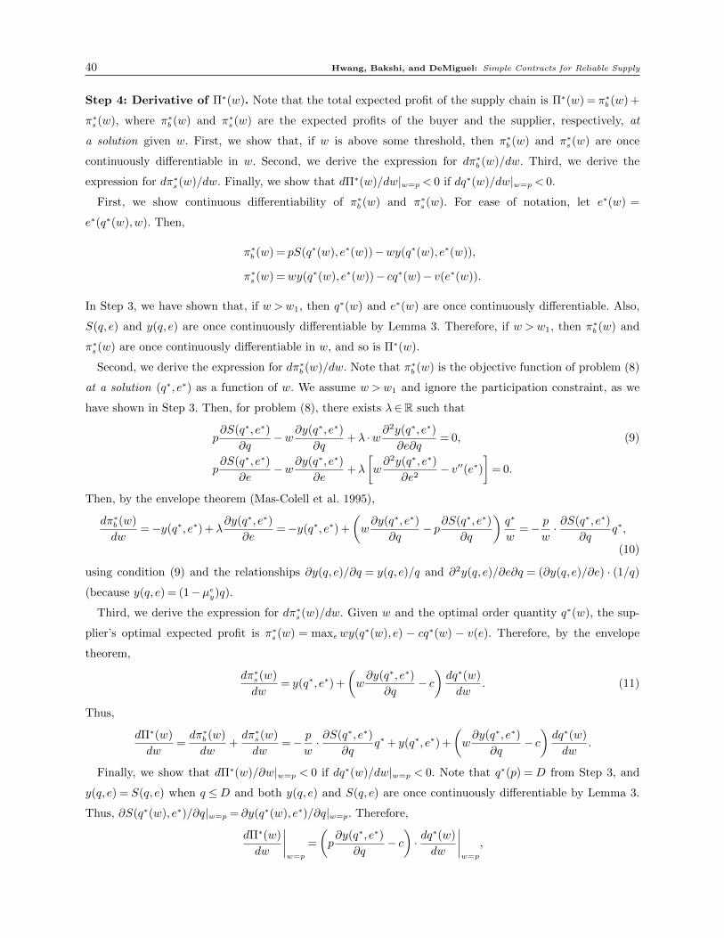
40 Hwang, Bakshi, and DeMiguel: Simple Contracts for Reliable Supply
Step 4: Derivative of Π∗(w). Note that the total expected profit of the supply chain is Π∗(w) = π∗b (w) +
π∗s (w), where π∗b (w) and π∗s (w) are the expected profits of the buyer and the supplier, respectively, at
a solution given w. First, we show that, if w is above some threshold, then π∗b (w) and π∗s (w) are once
continuously differentiable in w. Second, we derive the expression for dπ∗b (w)/dw. Third, we derive the
expression for dπ∗s (w)/dw. Finally, we show that dΠ∗(w)/dw|w=p < 0 if dq∗(w)/dw|w=p < 0.
First, we show continuous differentiability of π∗b (w) and π∗s (w). For ease of notation, let e∗(w) =
e∗(q∗(w),w). Then,
π∗b (w) = pS(q∗(w), e∗(w))−wy(q∗(w), e∗(w)),
π∗s (w) =wy(q∗(w), e∗(w))− cq∗(w)− v(e∗(w)).
In Step 3, we have shown that, if w >w1, then q∗(w) and e∗(w) are once continuously differentiable. Also,
S(q, e) and y(q, e) are once continuously differentiable by Lemma 3. Therefore, if w > w1, then π∗b (w) and
π∗s (w) are once continuously differentiable in w, and so is Π∗(w).
Second, we derive the expression for dπ∗b (w)/dw. Note that π∗b (w) is the objective function of problem (8)
at a solution (q∗, e∗) as a function of w. We assume w >w1 and ignore the participation constraint, as we
have shown in Step 3. Then, for problem (8), there exists λ∈R such that
p∂S(q∗, e∗)
∂q−w∂y(q∗, e∗)
∂q+λ ·w∂
2y(q∗, e∗)
∂e∂q= 0, (9)
p∂S(q∗, e∗)
∂e−w∂y(q∗, e∗)
∂e+λ
[w∂2y(q∗, e∗)
∂e2− v′′(e∗)
]= 0.
Then, by the envelope theorem (Mas-Colell et al. 1995),
dπ∗b (w)
dw=−y(q∗, e∗) +λ
∂y(q∗, e∗)
∂e=−y(q∗, e∗) +
(w∂y(q∗, e∗)
∂q− p∂S(q∗, e∗)
∂q
)q∗
w=− p
w· ∂S(q∗, e∗)
∂qq∗,
(10)
using condition (9) and the relationships ∂y(q, e)/∂q = y(q, e)/q and ∂2y(q, e)/∂e∂q = (∂y(q, e)/∂e) · (1/q)
(because y(q, e) = (1−µey)q).
Third, we derive the expression for dπ∗s (w)/dw. Given w and the optimal order quantity q∗(w), the sup-
plier’s optimal expected profit is π∗s (w) = maxewy(q∗(w), e) − cq∗(w) − v(e). Therefore, by the envelope
theorem,
dπ∗s (w)
dw= y(q∗, e∗) +
(w∂y(q∗, e∗)
∂q− c)dq∗(w)
dw. (11)
Thus,
dΠ∗(w)
dw=dπ∗b (w)
dw+dπ∗s (w)
dw=− p
w· ∂S(q∗, e∗)
∂qq∗+ y(q∗, e∗) +
(w∂y(q∗, e∗)
∂q− c)dq∗(w)
dw.
Finally, we show that dΠ∗(w)/∂w|w=p < 0 if dq∗(w)/dw|w=p < 0. Note that q∗(p) = D from Step 3, and
y(q, e) = S(q, e) when q ≤D and both y(q, e) and S(q, e) are once continuously differentiable by Lemma 3.
Thus, ∂S(q∗(w), e∗)/∂q|w=p = ∂y(q∗(w), e∗)/∂q|w=p. Therefore,
dΠ∗(w)
dw
∣∣∣∣w=p
=
(p∂y(q∗, e∗)
∂q− c)· dq
∗(w)
dw
∣∣∣∣w=p
,
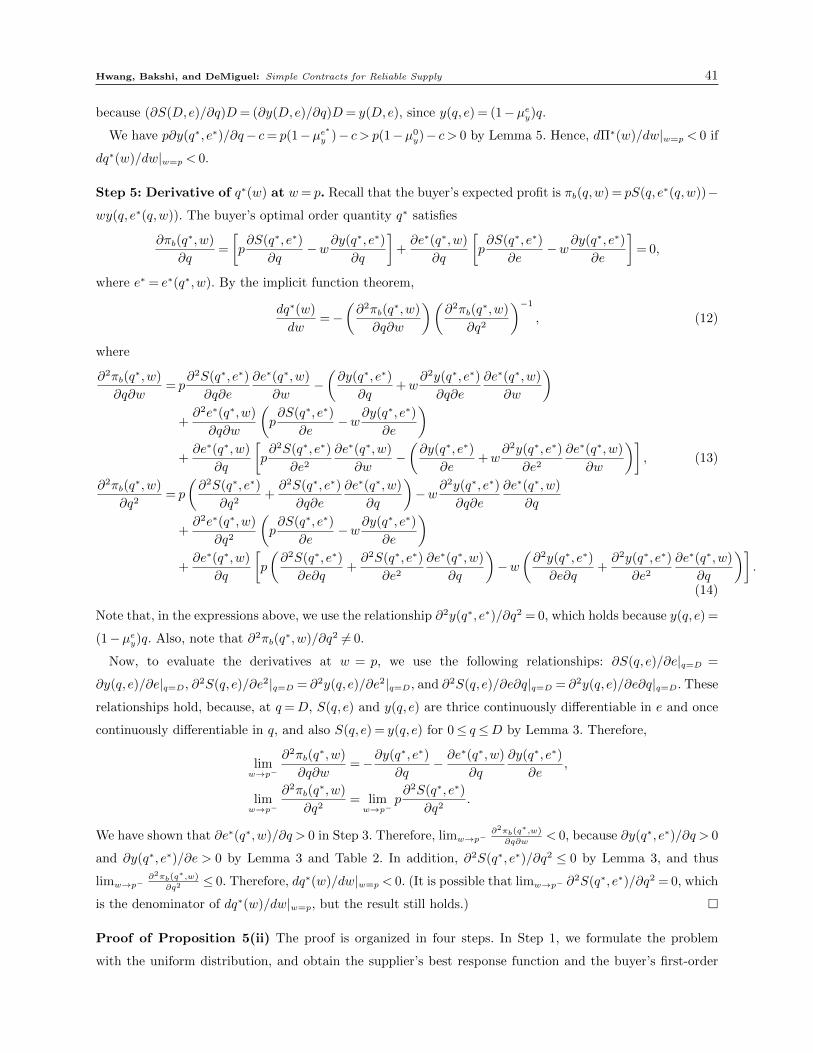
Hwang, Bakshi, and DeMiguel: Simple Contracts for Reliable Supply 41
because (∂S(D,e)/∂q)D= (∂y(D,e)/∂q)D= y(D,e), since y(q, e) = (1−µey)q.
We have p∂y(q∗, e∗)/∂q− c= p(1−µe∗y )− c > p(1−µ0y)− c > 0 by Lemma 5. Hence, dΠ∗(w)/dw|w=p < 0 if
dq∗(w)/dw|w=p < 0.
Step 5: Derivative of q∗(w) at w= p. Recall that the buyer’s expected profit is πb(q,w) = pS(q, e∗(q,w))−
wy(q, e∗(q,w)). The buyer’s optimal order quantity q∗ satisfies
∂πb(q∗,w)
∂q=
[p∂S(q∗, e∗)
∂q−w∂y(q∗, e∗)
∂q
]+∂e∗(q∗,w)
∂q
[p∂S(q∗, e∗)
∂e−w∂y(q∗, e∗)
∂e
]= 0,
where e∗ = e∗(q∗,w). By the implicit function theorem,
dq∗(w)
dw=−
(∂2πb(q
∗,w)
∂q∂w
)(∂2πb(q
∗,w)
∂q2
)−1
, (12)
where
∂2πb(q∗,w)
∂q∂w= p
∂2S(q∗, e∗)
∂q∂e
∂e∗(q∗,w)
∂w−(∂y(q∗, e∗)
∂q+w
∂2y(q∗, e∗)
∂q∂e
∂e∗(q∗,w)
∂w
)+∂2e∗(q∗,w)
∂q∂w
(p∂S(q∗, e∗)
∂e−w∂y(q∗, e∗)
∂e
)+∂e∗(q∗,w)
∂q
[p∂2S(q∗, e∗)
∂e2
∂e∗(q∗,w)
∂w−(∂y(q∗, e∗)
∂e+w
∂2y(q∗, e∗)
∂e2
∂e∗(q∗,w)
∂w
)], (13)
∂2πb(q∗,w)
∂q2= p
(∂2S(q∗, e∗)
∂q2+∂2S(q∗, e∗)
∂q∂e
∂e∗(q∗,w)
∂q
)−w∂
2y(q∗, e∗)
∂q∂e
∂e∗(q∗,w)
∂q
+∂2e∗(q∗,w)
∂q2
(p∂S(q∗, e∗)
∂e−w∂y(q∗, e∗)
∂e
)+∂e∗(q∗,w)
∂q
[p
(∂2S(q∗, e∗)
∂e∂q+∂2S(q∗, e∗)
∂e2
∂e∗(q∗,w)
∂q
)−w
(∂2y(q∗, e∗)
∂e∂q+∂2y(q∗, e∗)
∂e2
∂e∗(q∗,w)
∂q
)].
(14)
Note that, in the expressions above, we use the relationship ∂2y(q∗, e∗)/∂q2 = 0, which holds because y(q, e) =
(1−µey)q. Also, note that ∂2πb(q∗,w)/∂q2 6= 0.
Now, to evaluate the derivatives at w = p, we use the following relationships: ∂S(q, e)/∂e|q=D =
∂y(q, e)/∂e|q=D, ∂2S(q, e)/∂e2|q=D = ∂2y(q, e)/∂e2|q=D, and ∂2S(q, e)/∂e∂q|q=D = ∂2y(q, e)/∂e∂q|q=D. These
relationships hold, because, at q=D, S(q, e) and y(q, e) are thrice continuously differentiable in e and once
continuously differentiable in q, and also S(q, e) = y(q, e) for 0≤ q≤D by Lemma 3. Therefore,
limw→p−
∂2πb(q∗,w)
∂q∂w=−∂y(q∗, e∗)
∂q− ∂e∗(q∗,w)
∂q
∂y(q∗, e∗)
∂e,
limw→p−
∂2πb(q∗,w)
∂q2= limw→p−
p∂2S(q∗, e∗)
∂q2.
We have shown that ∂e∗(q∗,w)/∂q > 0 in Step 3. Therefore, limw→p−∂2πb(q∗,w)
∂q∂w< 0, because ∂y(q∗, e∗)/∂q > 0
and ∂y(q∗, e∗)/∂e > 0 by Lemma 3 and Table 2. In addition, ∂2S(q∗, e∗)/∂q2 ≤ 0 by Lemma 3, and thus
limw→p−∂2πb(q∗,w)
∂q2≤ 0. Therefore, dq∗(w)/dw|w=p < 0. (It is possible that limw→p− ∂
2S(q∗, e∗)/∂q2 = 0, which
is the denominator of dq∗(w)/dw|w=p, but the result still holds.) �
Proof of Proposition 5(ii) The proof is organized in four steps. In Step 1, we formulate the problem
with the uniform distribution, and obtain the supplier’s best response function and the buyer’s first-order
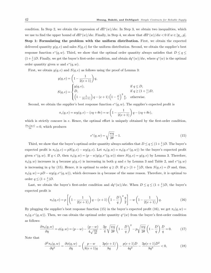
42 Hwang, Bakshi, and DeMiguel: Simple Contracts for Reliable Supply
condition. In Step 2, we obtain the expression of dΠ∗(w)/dw. In Step 3, we obtain two inequalities, which
we use to find the upper bound of dΠ∗(w)/dw. Finally, in Step 4, we show that dΠ∗(w)/dw < 0 if w ∈ [wc, p].
Step 1: Formulating the problem with the uniform distribution. First, we obtain the expected
delivered quantity y(q, e) and sales S(q, e) for the uniform distribution. Second, we obtain the supplier’s best
response function e∗(q,w). Third, we show that the optimal order quantity always satisfies that D ≤ q ≤(1+ 1
e)D. Finally, we get the buyer’s first-order condition, and obtain dq∗(w)/dw, where q∗(w) is the optimal
order quantity given w and e∗(q,w).
First, we obtain y(q, e) and S(q, e) as follows using the proof of Lemma 3:
y(q, e) =
(1− 1
2(e+ 1)
)q,
S(q, e) =
y(q, e), if q≤D,D, if q≥ (1 + 1
e)D,(
1− 12(e+1)
)q− (e+ 1)
(1− D
q
)2q
2, otherwise.
Second, we obtain the supplier’s best response function e∗(q,w). The supplier’s expected profit is
πs(q, e) =wy(q, e)− (cq+ θe) =w
(1− 1
2(e+ 1)
)q− (cq+ θe),
which is strictly concave in e. Hence, the optimal effort is uniquely obtained by the first-order condition,∂πs(q,e)
∂e= 0, which produces
e∗(q,w) =
√wq
2θ− 1. (15)
Third, we show that the buyer’s optimal order quantity always satisfies that D≤ q≤ (1+ 1e)D. The buyer’s
expected profit is πb(q, e) = pS(q, e)−wy(q, e). Let πb(q,w) = πb(q, e∗(q,w)) be the buyer’s expected profit
given e∗(q,w). If q < D, then πb(q,w) = (p−w)y(q, e∗(q,w)) since S(q, e) = y(q, e) by Lemma 3. Therefore,
πb(q,w) increases in q because y(q, e) is increasing in both q and e by Lemma 3 and Table 2, and e∗(q,w)
is increasing in q by (15). Hence, it is optimal to order q ≥D. If q > (1 + 1e)D, then S(q, e) =D and, thus,
πb(q,w) = pD−wy(q, e∗(q,w)), which decreases in q because of the same reason. Therefore, it is optimal to
order q≤ (1 + 1e)D.
Last, we obtain the buyer’s first-order condition and dq∗(w)/dw. When D ≤ q ≤ (1 + 1e)D, the buyer’s
expected profit is
πb(q, e) = p
[(1− 1
2(e+ 1)
)q− (e+ 1)
(1− D
q
)2q
2
]−w
(1− 1
2(e+ 1)
)q. (16)
By plugging the supplier’s best response function (15) in the buyer’s expected profit (16), we get πb(q,w) =
πb(q, e∗(q,w)). Then, we can obtain the optimal order quantity q∗(w) from the buyer’s first-order condition
as follows:
∂πb(q,w)
∂q= φ(q,w) = (p−w)− (p−w)
4√
wq
2θ
− 3p
4
√wq
2θ
(1− D
q
)2
− p√wq
2θ
(1− D
q
)D
q= 0. (17)
Note that
∂2πb(q,w)
∂q2=∂φ(q,w)
∂q=
(p−w
8(e+ 1)q− 3p(e+ 1)
8q
)− p(e+ 1)D
4q2− 3p(e+ 1)D2
8q3< 0, (18)
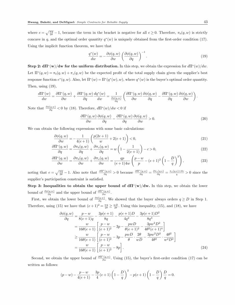
Hwang, Bakshi, and DeMiguel: Simple Contracts for Reliable Supply 43
where e=√
wq
2θ− 1, because the term in the bracket is negative for all e≥ 0. Therefore, πb(q,w) is strictly
concave in q, and the optimal order quantity q∗(w) is uniquely obtained from the first-order condition (17).
Using the implicit function theorem, we have that
q∗(w)
dw=−∂φ(q,w)
∂w
(∂φ(q,w)
∂q
)−1
. (19)
Step 2: dΠ∗(w)/dw for the uniform distribution. In this step, we obtain the expression for dΠ∗(w)/dw.
Let Π∗(q,w) = πb(q,w) + πs(q,w) be the expected profit of the total supply chain given the supplier’s best
response function e∗(q,w). Also, let Π∗(w) = Π∗(q∗(w),w), where q∗(w) is the buyer’s optimal order quantity.
Then, using (19),
dΠ∗(w)
dw=∂Π∗(q,w)
∂w+∂Π∗(q,w)
∂q
dq∗(w)
dw=
1∂φ(q,w)
∂q
(∂Π∗(q,w)
∂w
∂φ(q,w)
∂q− ∂Π∗(q,w)
∂q
∂φ(q,w)
∂w
).
Note that ∂φ(q,w)
∂q< 0 by (18). Therefore, dΠ∗(w)/dw < 0 if
∂Π∗(q,w)
∂w
∂φ(q,w)
∂q− ∂Π∗(q,w)
∂q
∂φ(q,w)
∂w> 0. (20)
We can obtain the following expressions with some basic calculations:
∂φ(q,w)
∂w=− 1
4(e+ 1)
(p(2e+ 1)
w+ 2(e+ 1)
)< 0, (21)
∂Π∗(q,w)
∂q=∂πb(q,w)
∂q+∂πs(q,w)
∂q=w
(1− 1
2(e+ 1)
)− c > 0, (22)
∂Π∗(q,w)
∂w=∂πb(q,w)
∂w+∂πs(q,w)
∂w=
qp
(e+ 1)4w
(p−wp− (e+ 1)2
(1− D
q
)2), (23)
noting that e =√
wq
2θ− 1. Also note that ∂Π∗(q,w)
∂q> 0 because ∂Π∗(q,w)
∂q= ∂πs(q,e)
∂q= πs(q,e)+θe
q> 0 since the
supplier’s participation constraint is satisfied.
Step 3: Inequalities to obtain the upper bound of dΠ∗(w)/dw. In this step, we obtain the lower
bound of ∂φ(q,w)
∂qand the upper bound of ∂Π∗(q,w)
∂w.
First, we obtain the lower bound of ∂φ(q,w)
∂q. We showed that the buyer always orders q ≥D in Step 1.
Therefore, using (15) we have that (e+ 1)2 = wq
2θ≥ wD
2θ. Using this inequality, (15), and (18), we have
∂φ(q,w)
∂q=
p−w8(e+ 1)q
− 3p(e+ 1)
8q− p(e+ 1)D
4q2− 3p(e+ 1)D2
8q3
=w
16θ(e+ 1)
[p−w
(e+ 1)2− 3p− pwD
θ(e+ 1)2− 3pw2D2
4θ2(e+ 1)4
]≥ w
16θ(e+ 1)
[p−w
(e+ 1)2− 3p− pwD
θ· 2θ
wD− 3pw2D2
4θ2· 4θ2
w2D2
]=
w
16θ(e+ 1)
[p−w
(e+ 1)2− 8p
]. (24)
Second, we obtain the upper bound of ∂Π∗(q,w)
∂w. Using (15), the buyer’s first-order condition (17) can be
written as follows:
(p−w)− p−w4(e+ 1)
− 3p
4(e+ 1)
(1− D
q
)2
− p(e+ 1)
(1− D
q
)D
q= 0.
44 Hwang, Bakshi, and DeMiguel: Simple Contracts for Reliable Supply
Rearranging this first-order condition, we get(1− D
q
)[3p
4
(1− D
q
)+ p
D
q
]= (p−w)
[1
e+ 1− 1
4(e+ 1)2
].
Therefore, (1− D
q
)=
4q
3q+D
(1− w
p
)[1
e+ 1− 1
4(e+ 1)2
]≥ 4q
3q+ q
(1− w
p
)[1
e+ 1− 1
4(e+ 1)2
]=
(1− w
p
)1
(e+ 1)
[1− 1
4(e+ 1)
]≥ 3
4
(1− w
p
)1
(e+ 1),
where the second step holds because q≥D and the last step holds because e≥ 0.
Now using this result, (15), and (23), we have
∂Π∗(q,w)
∂w=
p
(e+ 1)4w· 2θ(e+ 1)2
w
[(1− w
p
)− (e+ 1)2
(1− D
q
)2]
=pθ(e+ 1)
2w2
[(1− w
p
)− (e+ 1)2
(1− D
q
)2]
≤ pθ(e+ 1)
2w2
[(1− w
p
)− (e+ 1)2 9
16
(1− w
p
)21
(e+ 1)2
]
=θ(e+ 1)(p−w)
2w2
(7p+ 9w
16p
). (25)
Step 4: Monotonicity. In this step, we show that dΠ∗(w)/dw < 0 if w ∈ [wc, p]. In Step 2, we already
showed that dΠ∗(w)/dw < 0 if (20) holds. Note that if ∂Π∗(q,w)
∂w< 0, then (20) always holds, because we have
∂φ(q,w)
∂q< 0, ∂Π∗(q,w)
∂q> 0, and ∂φ(q,w)
∂w< 0 from Steps 1 and 2.
If ∂Π∗(q,w)
∂w> 0, then using the lower bound of ∂φ(q,w)
∂q, (24), and the upper bound of ∂Π∗(q,w)
∂w, (25), along
with (21) and (22), we have that
∂Π
∂w
∂φ
∂q− ∂Π
∂q
∂φ
∂w≥ θ(e+ 1)(p−w)
2w2· 7p+ 9w
16p· w
16θ(e+ 1)
(p−w
(e+ 1)2− 8p
)+
[w
(1− 1
2(e+ 1)
)− c]·[
1
4(e+ 1)
(p(2e+ 1)
w+ 2(e+ 1)
)]=
(p−w)2(7p+ 9w)
512wp(e+ 1)2− (p−w)(7p+ 9w)
64w
+p
8
(2e+ 1
e+ 1
)2
+w
4
(2e+ 1
e+ 1
)− cp
4w
(2e+ 1
e+ 1
)− c
2
≥− (p−w)(7p+ 9w)
64w+p
8
(2e+ 1
e+ 1
)2
+w
4
(2e+ 1
e+ 1
)− cp
4w
(2e+ 1
e+ 1
)− c
2.
We have that e+ 1 =√
wq
2θ≥√
cD2θ
, because w≥ c and q≥D. Therefore,
2−√
2θ
cD≤ 2e+ 1
e+ 1= 2− 1
e+ 1< 2.
Hwang, Bakshi, and DeMiguel: Simple Contracts for Reliable Supply 45
Let k= 2−√
2θcD
. Then, we have that
∂Π
∂w
∂φ
∂q− ∂Π
∂q
∂φ
∂w≥− (p−w)(7p+ 9w)
64w+p
8
(2e+ 1
e+ 1
)2
+w
4
(2e+ 1
e+ 1
)− cp
4w
(2e+ 1
e+ 1
)− c
2
>− (p−w)(7p+ 9w)
64w+p
8k2 +
w
4k− pc
2w− c
2
=1
64w
[(16k+ 9)w2 + (8pk2− 32c− 2p)w− p(7p+ 32c)
].
Therefore, using the solution of the quadratic equation in the square bracket, ∂Π∂w
∂φ
∂q− ∂Π
∂q
∂φ
∂w> 0 if
w≥wc =−(8pk2− 32c− 2p) +
√(8pk2− 32c− 2p)2 + 4p(16k+ 9)(7p+ 32c)
2(16k+ 9).
�
Proof of Proposition 5(iii) The proof is organized in four steps. In Step 1, we show some properties of
the cost of effort v(e) = θem with respect to θ and m. In Step 2, we show some properties of the supplier’s
best response function e∗(q,w) with respect to θ and m. In Step 3, we obtain the upper bound of dq∗(w)/dw
using the properties from the previous steps. Finally, in Step 4, we show that the efficiency is decreasing if
either θ or m is large enough.
Step 1: Properties of the cost of effort. We show the following four properties of v(e) at the equilibrium
effort e∗: limθ→∞ v′′(e∗) =∞, limm→∞ v
′′(e∗) =∞, limθ→∞v′′′(e∗)
(v′′(e∗))3= 0, and limm→∞
v′′′(e∗)(v′′(e∗))3
= 0.
First, we show that limθ→∞ v′′(e∗) =∞. The supplier’s first-order condition is the following.
∂πs(q∗, e∗)
∂e=w
∂y(q∗, e∗)
∂e− v′(e∗) =w
∂y(q∗, e∗)
∂e− θme∗m−1 = 0. (26)
Therefore, θ= wm
∂y(q∗,e∗)∂e
e∗1−m. Note that ∂y(q,e)
∂eis decreasing in e since ∂2y(q,e)
∂e2< 0 by Lemma 3 and Table 2
and finite by Assumption 3, and also e1−m is decreasing in e since m > 1. Hence, it is easy to see that
limθ→∞ e∗ = 0. Thus, using (26),
limθ→∞
v′′(e∗) = limθ→∞
θm(m− 1)e∗m−2 = lime∗→0
w∂y(q∗, e∗)
∂e(m− 1)
1
e∗=∞, (27)
since ∂y(q,e)
∂e> 0, e≥ 0 by Lemma 3 and Table 2.
Second, we show that limm→∞ v′′(e∗) = ∞. Note that limm→∞ e
∗ < ∞, because the first-order condi-
tion (26) cannot hold otherwise because of the following reason: w ∂y(q∗,e∗)∂e
is finite by Assumption 3, but
limm→∞ θme∗m−1 =∞ if limm→∞ e
∗ =∞. Therefore,
limm→∞
v′′(e∗) = limm→∞
w∂y(q∗, e∗)
∂e(m− 1)
1
e∗=∞. (28)
Third, we show that limθ→∞v′′′(e∗)
(v′′(e∗))3= 0. Using the first-order condition (26),
limθ→∞
v′′′(e∗)
(v′′(e∗))3= limθ→∞
θm(m− 1)(m− 2)e∗m−3
θ3m3(m− 1)3e∗3m−6= limθ→∞
(m− 2)(w ∂y(q∗,e∗)
∂e
)2
(m− 1)2
e∗ = 0, (29)
because ∂y(q,e)
∂e> 0, e≥ 0 by Lemma 3 and Table 2, and limθ→∞ e
∗ = 0.
Last, we show that limm→∞v′′′(e∗)
(v′′(e∗))3= 0.
limm→∞
v′′′(e∗)
(v′′(e∗))3= limm→∞
(m− 2)(w ∂y(q∗,e∗)
∂e
)2
(m− 1)2
e∗ = 0, (30)
46 Hwang, Bakshi, and DeMiguel: Simple Contracts for Reliable Supply
since limm→∞ e∗ <∞.
Step 2: Properties of the best response function. We show the supplier’s best response
function e∗(q∗,w) satisfies the following properties: limθ→∞∂e∗(q∗,w)
∂q= limm→∞
∂e∗(q∗,w)
∂q= 0,
limθ→∞∂e∗(q∗,w)
∂w= limm→∞
∂e∗(q∗,w)
∂w= 0, limθ→∞
∂2e∗(q∗,w)
∂q2= limm→∞
∂2e∗(q∗,w)
∂q2= 0, and limθ→∞
∂2e∗(q∗,w)
∂q∂w=
limm→∞∂2e∗(q∗,w)
∂q∂w= 0.
First, we show that limθ→∞∂e∗(q∗,w)
∂q= limm→∞
∂e∗(q∗,w)
∂q= 0. We can obtain ∂e∗(q∗,w)
∂qby differentiating the
first-order condition (26) with respect to q as follows:
w∂2y(q∗, e∗)
∂e∂q+
(w∂2y(q∗, e∗)
∂e2− v′′(e∗)
)∂e∗(q∗,w)
∂q= 0. (31)
Therefore,
∂e∗(q∗,w)
∂q=−
w ∂2y(q∗,e∗)∂e∂q
w ∂2y(q∗,e∗)∂e2
− v′′(e∗). (32)
Thus, limθ→∞∂e∗(q∗,w)
∂q= limm→∞
∂e∗(q∗,w)
∂q= 0 using (27) and (28), because y(q, e) has finite derivatives
regardless of e by Assumption 3.
Second, we show that limθ→∞∂e∗(q∗,w)
∂w= limm→∞
∂e∗(q∗,w)
∂w= 0. Using the first-order condition (26) and
the implicit function theorem, we have
∂e∗(q∗,w)
∂w=−
∂y(q∗,e∗)∂e
w ∂2y(q∗,e∗)∂e2
− v′′(e∗). (33)
Therefore, limθ→∞∂e∗(q∗,w)
∂w= limm→∞
∂e∗(q∗,w)
∂w= 0 using (27) and (28), because y(q, e) has finite derivatives
regardless of e by Assumption 3. Note that we can observe the following relationship between (32) and (33):
∂e∗(q∗,w)
∂w=q
w
∂e∗(q∗,w)
∂q, (34)
where ∂2y(q,e)
∂e∂q= ∂y(q,e)
∂e· 1q
because y(q, e) is linear in q.
Third, we show that limθ→∞∂2e∗(q∗,w)
∂q2= limm→∞
∂2e∗(q∗,w)
∂q2= 0. We can obtain ∂2e∗(q∗,w)
∂q2by differentiating
(31) with respect to q as follows.
w · ∂3y(q∗, e∗)
∂e2∂q
∂e∗(q∗,w)
∂q+
[(w∂3y(q∗, e∗)
∂e3− v′′′(e∗)
)∂e∗(q∗,w)
∂q+w
∂3y(q∗, e∗)
∂e2∂q
]∂e∗(q∗,w)
∂q
+
(w∂2y(q∗, e∗)
∂e2− v′′(e∗)
)∂2e∗(q∗,w)
∂q2= 0,
where ∂3y(q∗,e∗)∂e∂q2
= 0, because y(q, e) is linear in q. Therefore,
∂2e∗(q∗,w)
∂q2=−
2w ∂3y(q∗,e∗)∂e2∂q
+(w ∂3y(q∗,e∗)
∂e3− v′′′(e∗)
)∂e∗(q∗,w)
∂q
w ∂2y(q∗,e∗)∂e2
− v′′(e∗)· ∂e
∗(q∗,w)
∂q
=−2w ∂2y(q∗,e∗)
∂e2· 1q∗
w ∂2y(q∗,e∗)∂e2
− v′′(e∗)· ∂e
∗(q∗,w)
∂q−
w ∂3y(q∗,e∗)∂e3
− v′′′(e∗)(w ∂2y(q∗,e∗)
∂e2− v′′(e∗)
)3 ·(w∂2y(q∗, e∗)
∂e∂q
)2
,
where ∂3y(q,e)
∂e2∂q= ∂2y(q,e)
∂e21q
because y(q, e) is linear in q, and also we use (32). Therefore, we can see that
limθ→∞∂2e∗(q∗,w)
∂q2= 0 and limm→∞
∂2e∗(q∗,w)
∂q2= 0 using (27), (28), (29), (30), and that limθ→∞
∂e∗(q∗,w)
∂q=
limm→∞∂e∗(q∗,w)
∂q= 0. Note that y(q, e) has finite derivatives regardless of e by Assumption 3.
Hwang, Bakshi, and DeMiguel: Simple Contracts for Reliable Supply 47
Finally, we show that limθ→∞∂2e∗(q∗,w)
∂q∂w= limm→∞
∂2e∗(q∗,w)
∂q∂w= 0. We can obtain ∂2e∗(q∗,w)
∂q∂wby differentiating
(31) with respect to w as follows.[∂2y(q∗, e∗)
∂e2+
(w∂3y(q∗, e∗)
∂e3− v′′′(e∗)
)e∗(q∗,w)
∂w
]∂e∗(q∗,w)
∂q
+
(w∂2y(q∗, e∗)
∂e2− v′′(e∗)
)∂2e∗(q∗,w)
∂q∂w+
(∂2y(q∗, e∗)
∂e∂q+w
∂3y(q∗, e∗)
∂e2∂q
∂e∗(q∗,w)
∂w
)= 0.
Therefore,
∂2e∗(q∗,w)
∂q∂w=−
∂2y(q∗,e∗)∂e∂q
+w ∂3y(q∗,e∗)∂e2∂q
∂e∗(q∗,w)
∂w+[∂2y(q∗,e∗)
∂e2+(w ∂3y(q∗,e∗)
∂e3− v′′′(e∗)
)∂e∗(q∗,w)
∂w
]∂e∗(q∗,w)
∂q
w ∂2y(q∗,e∗)∂e2
− v′′(e∗)
=−∂2y(q∗,e∗)
∂e∂q+ 2 ∂
2y(q∗,e∗)∂e2
∂e∗(q∗,w)
∂q
w ∂2y(q∗,e∗)∂e2
− v′′(e∗)−
q∗
w
(w ∂3y(q∗,e∗)
∂e3− v′′′(e∗)
)(w ∂2y(q∗,e∗)
∂e∂q
)2
(w ∂2y(q∗,e∗)
∂e2− v′′(e∗)
)3 ,
using (32) and (34), and that ∂3y(q,e)
∂e2∂q= ∂2y(q,e)
∂e2· 1q
because y(q, e) is linear in q. Again, we can observe
that limθ→∞∂2e∗(q∗,w)
∂q∂w= limm→∞
∂2e∗(q∗,w)
∂q∂w= 0, using (27), (28), (29), (30), and that limθ→∞
∂e∗(q∗,w)
∂q=
limm→∞∂e∗(q∗,w)
∂q= 0. Note that y(q, e) has finite derivatives regardless of e by Assumption 3.
Step 3: Upper bound of dq∗(w)/dw. Using the results on limits of e∗(q∗,w) from Step 2, and using (13)
and (14), we have
limθ→∞
∂2πb(q∗,w)
∂q∂w= limm→∞
∂2πb(q∗,w)
∂q∂w=−∂y(q∗, e∗)
∂q,
limθ→∞
∂2πb(q∗,w)
∂q2= limm→∞
∂2πb(q∗,w)
∂q2= p
∂2S(q∗, e∗)
∂q2.
Hence, for any arbitrarily small ε > 0, there exists θ′ > 0 such that for all θ > θ′, we have that
−∂y(q∗, e∗)
∂q− ε <∂
2πb(q∗,w)
∂q∂w<−∂y(q∗, e∗)
∂q+ ε,
p∂2S(q∗, e∗)
∂q2− ε <∂
2πb(q∗,w)
∂q2< p
∂2S(q∗, e∗)
∂q2+ ε.
Also, for any arbitrarily small ε > 0, there exists m′ > 1 such that for all m>m′, the same holds. Then,
using (12), we can obtain the following upper bound for dq∗(w)/dw:
dq∗(w)
dw=−
(∂2πb(q
∗,w)
∂q∂w
)(∂2πb(q
∗,w)
∂q2
)−1
<
∂y(q∗,e∗)∂q
− ε
p ∂2S(q∗,e∗)∂q2
− ε,
where ∂y(q∗,e∗)∂q
> 0 and ∂2S(q∗,e∗)∂q2
< 0 by Lemma 3 and Table 2.
Step 4: Decreasing efficiency. From equations (10) and (11), we have
dΠ∗(w)
dw=dπ∗b (w)
dw+dπ∗s (w)
dw= λ
∂y(q∗, e∗)
∂e+
(w∂y(q∗, e∗)
∂q− c)dq∗(w)
dw.
Using the results from Step 3 and the second equation in (9) for λ, for any ε > 0 if θ or m> 1 is large
enough, we get the following inequality.
dΠ∗(w)
dw= λ
∂y(q∗, e∗)
∂e+
(w∂y(q∗, e∗)
∂q− c)dq∗(w)
dw
=−p ∂S(q∗,e∗)
∂e−w ∂y(q∗,e∗)
∂e
w ∂2y(q∗,e∗)∂e2
− v′′(e)· ∂y(q∗, e∗)
∂e+
(w∂y(q∗, e∗)
∂q− c)dq∗(w)
dw
<−p ∂S(q∗,e∗)
∂e−w ∂y(q∗,e∗)
∂e
w ∂2y(q∗,e∗)∂e2
− v′′(e∗)· ∂y(q∗, e∗)
∂e+
(w∂y(q∗, e∗)
∂q− c) ∂y(q∗,e∗)
∂q− ε
p ∂2S(q∗,e∗)∂q2
− ε, (35)
48 Hwang, Bakshi, and DeMiguel: Simple Contracts for Reliable Supply
where w ∂y(q∗,e∗)∂q
− c = (wy(q∗, e∗) − cq) 1q
= (πs(q∗, e∗) + v(e∗)) 1
q> 0, since y(q, e) is linear in q and the
supplier’s participation constraint is satisfied.
Note that the first term in (35) tends to zero as θ→∞ or as m→∞, because ∂S(q,e)
∂e, ∂y(q,e)
∂e, and ∂2y(q,e)
∂e2
have finite bounds regardless of e by Assumption 3, and limθ→∞ v′′(e∗) = limm→∞ v
′′(e∗) =∞ by (27) and
(28). Also, we can find a sufficiently small ε > 0 such that the second term is negative, because(w∂y(q∗, e∗)
∂q− c) ∂y(q∗,e∗)
∂q
p ∂2S(q∗,e∗)∂q2
< 0,
where ∂y(q∗,e∗)∂q
> 0 and ∂2S(q∗,e∗)∂q2
< 0 by Lemma 3 and Table 2. Therefore, 1) there exists θ′ such that for all
θ > θ′, dΠ∗(w)
dw< 0 for all w, and 2) there exists m′ > 1 such that for all m>m′, dΠ∗(w)
dw< 0 for all w. �
Proof of Proposition 6 Under a unit-penalty with buy-back contract (w,z, b), each firm’s expected profit
is as follows:
πb(q, e,w, z, b) = pS(q, e)−wy(q, e) + z(q− y(q, e)) + b(y(q, e)−S(q, e)),
πs(q, e,w, z, b) =wy(q, e)− z(q− y(q, e))− b(y(q, e)−S(q, e))− c(q, e).
For χ ∈[0, Π(qo,eo)
Π(qo,eo)+v(eo)
], the coordinating contract parameters are w∗ = p(1 − χ) + χ(µe
o
y M + c), z∗ =
χ((1−µeoy )M − c), and b∗ = p(1−χ), where M = v′(eo)/(∂y(qo, eo)/∂e).
The proof is organized in two steps. In Step 1, we reformulate problem (2). In Step 2, we show that the
contract (w∗, z∗, b∗) satisfies the KKT conditions at (qo, eo).
Step 1: Reformulation. In problem (2), we can replace the first constraint with its first-order condition. The
supplier’s expected profit is πs(q, e,w∗, z∗, b∗) = (w∗+z∗− b∗)y(q, e)+ b∗S(q, e)−z∗q− (cq+v(e)), and this is
strictly concave in e because of the following reason. First, w∗+ z∗− b∗ = χM = χv′(eo)/(∂y(qo, eo)/∂e)≥ 0,
because χ≥ 0, v′(eo)> 0 by Assumption 3 and ∂y(qo, eo)/∂e > 0 by Lemma 3 and Table 2. Second, y(q, e)
and S(q, e) are both strictly concave in e by Lemma 3 and Table 2. Third, v(e) is convex by Assumption 3.
Also, by Assumption 3, we focus only on the interior solutions. Therefore, problem (2) can be reformulated
as
maxq,e
πb(q, e,w∗, z∗, b∗), (36)
s.t.∂πs(q, e,w
∗, z∗, b∗)
∂e= 0,
πs(q, e,w∗, z∗, b∗)≥ 0.
Step 2: KKT conditions. Assume (qo, eo) is a solution to problem (36). Then, there exist λ,µ ∈ R such
that
∂πb(qo, eo,w∗, z∗, b∗)
∂q+λ
∂2πs(qo, eo,w∗, z∗, b∗)
∂e∂q+µ
∂πs(qo, eo,w∗, z∗, b∗)
∂q= 0,
∂πb(qo, eo,w∗, z∗, b∗)
∂e+λ
∂2πs(qo, eo,w∗, z∗, b∗)
∂e2+µ
∂πs(qo, eo,w∗, z∗, b∗)
∂e= 0,
where µ ·πs(qo, eo,w∗, z∗, b∗) = 0 and µ≥ 0. Also, (qo, eo) satisfies the two constraints.
Note that, under the contract (w∗, z∗, b∗), each firm’s expected profit is the following:
Hwang, Bakshi, and DeMiguel: Simple Contracts for Reliable Supply 49
πs(q, e,w∗, z∗, b∗) = χMy(q, e) + p(1−χ)S(q, e)−χ((1−µeoy )M − c)q− (cq+ v(e)),
πb(q, e,w∗, z∗, b∗) = pχS(q, e)−χMy(q, e) +χ((1−µeoy )M − c)q,
where M = v′(eo) · (∂y(qo, eo)/∂e)−1.
From the first KKT condition, we have[pχ∂S(qo, eo)
∂q−χM ∂y(qo, eo)
∂q+χ
((1−µeoy )M − c
)]+λ
[χM
∂2y(qo, eo)
∂e∂q+ p(1−χ)
∂2S(qo, eo)
∂e∂q
]+µ
[χM
∂y(qo, eo)
∂q+ p(1−χ)
∂S(qo, eo)
∂q−χ
((1−µeoy )M − c
)− c]
= 0.
Simple arithmetic calculations reveal that the first and the third square brackets are zero, because
∂y(qo, eo)/∂q = (1− µeoy ), and also p∂S(qo, eo)/∂q = c by the first-order condition of the centralized supply
chain. In addition, for the second square bracket, note that M∂2y(qo, eo)/∂e∂q=M(∂y(qo, eo)/∂e) · (1/qo) =
v′(eo)/qo, because y(q, e) = (1−µey)q. Therefore, we have
λ
[χv′(eo)
1
qo+ p(1−χ)
∂2S(qo, eo)
∂e∂q
]= 0.
Let λ= 0. Then, the first condition is always satisfied. From the second KKT condition, we have[pχ∂S(qo, eo)
∂e−χM ∂y(qo, eo)
∂e
]+λ
[χM
∂2y(qo, eo)
∂e2+ p(1−χ)
∂2S(qo, eo)
∂e2− v′′(eo)
]+µ
[χM
∂y(qo, eo)
∂e+ p(1−χ)
∂S(qo, eo)
∂e− v′(eo)
]= 0.
The second square bracket disappears, because λ= 0. Simple arithmetic calculations reveal that the first and
the third square brackets are zero, because M ·∂y(qo, eo)/∂e= v′(eo), and also p∂S(qo, eo)/∂e= v′(eo) by the
first-order condition of the centralized supply chain. Therefore, the second KKT condition holds regardless
of µ, and thus µ · πs(qo, eo,w∗, z∗, b∗) = 0 is also satisfied. (We can simply set µ= 0 if the second constraint
does not bind.) Thus, the second constraint may or may not bind. Also, it is easy to check that the two
constraints are satisfied at (qo, eo). Therefore, KKT conditions are satisfied at (qo, eo).
The buyer’s expected profit is πb(q∗, e∗,w∗, z∗, b∗) = χ(Π(qo, eo)+v(eo)), and the supplier’s expected profit
is πs(q∗, e∗,w∗, z∗, b∗) = (1−χ)Π(qo, eo)−χv(eo). �
Proof of Proposition 7 The proof is organized as follows. From Step 1 to 4, we ignore the participation
constraint in problem (2), but in Step 5, we show that the participation constraint is always satisfied if w is
above some threshold.
• Step 1: There exists w0 < p such that for all w ∈ [w0, p], the supplier’s optimal production quantity x∗
and effort e∗ always satisfy 0< 1− q/x∗ <ay(e∗) for any q. From the next step, we focus on w ∈ [w0, p].
• Step 2: The supplier’s best response functions x(q) and e(q) are once continuously differentiable with
x′(q)> 0 and e′(q)> 0.
• Step 3: The buyer’s optimal order quantity q∗ satisfies q∗ ≥D regardless of the wholesale price.
• Step 4: There exists w1 < p such that the optimal order quantity is q∗ =D if w ∈ [w1, p].
• Step 5: There exists w2 < p such that if w ∈ [w2, p], then the participation constraint is always satisfied.
• Step 6: If q∗ =D, the efficiency of the supply chain strictly increases in w.
50 Hwang, Bakshi, and DeMiguel: Simple Contracts for Reliable Supply
Then, if we set wd = max{w0,w1,w2}, the statement holds.
Step 1: Feasible region. First, we show that x∗ > q by contradiction. If x∗ ≤ q, then y(q,x∗, e∗) = (1−µe∗
y )x∗. We know that p(1−µey)− c > 0 for all e≥ 0 by Lemma 5. Therefore, we can find w0 < p such that,
for all w ∈ [w0, p], ∂πs(q,x, e)/∂x=w(1−µey)− c > 0 for all e≥ 0. Then, the first-order condition cannot be
satisfied. Hence, x∗ > q, or 0< 1− q/x∗, when w ∈ [w0, p].
Second, we show that 1−q/x∗ <ay(e∗) by contradiction. When x> q, we have ∂y(q,x, e)/∂x= (1−ay(e))+∫ ay(e)
1−q/xH(ξ | e)dξ− q
xH(1− q/x | e). If 1− q/x∗ ≥ ay(e∗), then ∂y(q,x∗, e∗)/∂x= 0 because H(ay(e
∗) | e∗) = 1.
Therefore, the first-order condition cannot be satisfied, and thus 0< 1− q/x∗ <ay(e∗).Step 2: Best response functions. The supplier’s best response functions are obtained by the following
first-order conditions:
w∂y(q,x, e)
∂x− c= 0, w
∂y(q,x, e)
∂e− v′(e) = 0. (37)
The first equation always holds when w ∈ [w0, p] by Step 1. The second equation may not hold for any e≥ 0
if q is small, in which case e(q) = 0 and
x′(q) =−w∂2y(q,x, e)/∂x∂q
w∂2y(q,x, e)/∂x2,
by the implicit function theorem. Hence, x′(q)> 0 because ∂2y(q,x,e)
∂x∂q> 0 and ∂2y(q,x,e)
∂x2< 0 (which we show
later in this step). We assume that the second equation in (37) always holds if q ≥D, which is in line with
Assumption 3 of focusing on interior solutions.
Now, assume both first-order conditions hold. The determinant of the Jacobian of the two first-order
conditions is strictly positive, that is, w2(∂2y
∂x2∂2y
∂e2− ( ∂2y
∂x∂e)2)−w ∂2y
∂x2v′′(e)> 0, with a slight abuse of notation
using y for y(q,x, e). This is because y(q,x, e) is jointly concave in x and e by Assumption 4, and thus∂2y
∂x2∂2y
∂e2− ( ∂2y
∂x∂e)2 > 0, and also ∂2y/∂x2 ≤ 0 by Lemma 4 and v′′(e)≥ 0 by Assumption 3. Therefore, by the
implicit function theorem, x(q) and e(q) are once continuously differentiable. (Also note that y(q,x, e) is
thrice continuously differentiable in x and e by Lemma 4, and v(e) is thrice continuously differentiable by
Assumption 3.)
Hence, [x′(q)e′(q)
]=−
[w ∂2y
∂x2, w ∂2y
∂x∂e
w ∂2y
∂e∂x, w ∂2y
∂e2− v′′(e)
]−1
·
[w ∂2y
∂x∂q
w ∂2y
∂e∂q
]
=− 1
w2
(∂2y
∂x2∂2y
∂e2− ( ∂2y
∂x∂e)2
)−w ∂2y
∂x2v′′(e)
·
w ∂2y
∂x∂q
(w ∂2y
∂e2− v′′(e)
)−w2 ∂2y
∂x∂e
∂2y
∂e∂q
w2(∂2y
∂x2∂2y
∂e∂q− ∂2y
∂x∂e
∂2y
∂x∂q
) . (38)
Because we already know the sign of the determinant of the Jacobian, we only need to check the signs
of the two components in the matrix in (38). But before we proceed, we need to obtain the derivatives of
y(q,x, e) and find some important relationships that we use in checking the signs of x′(q) and e′(q). We have
y(q,x, e) = [(1− ay(e)) +∫ ay(e)
1−q/xH(ξ | e)dξ]x. We obtain the following derivatives:
∂y(q,x, e)
∂e= x
∫ ay(e)
1−q/x
∂H(ξ | e)∂e
dξ > 0,∂2y(q,x, e)
∂e∂q=∂H(1− q
x| e)
∂e> 0,
∂2y(q,x, e)
∂x∂q=
q
x2h(
1− q
x| e)> 0,
∂2y(q,x, e)
∂q2=− 1
xh(
1− q
x| e)< 0,
∂2y(q,x, e)
∂x∂e=
∫ ay(e)
1−q/x
∂H(ξ | e)∂e
dξ− q
x
∂H(1− q
x| e)
∂e,
∂2y(q,x, e)
∂x2=− q
2
x3h(
1− q
x| e)< 0,
Hwang, Bakshi, and DeMiguel: Simple Contracts for Reliable Supply 51
where we can obtain the signs because h(ξ | e)> 0 and ∂H(ξ | e)/∂e > 0 when ξ ∈ (0, ay(e)) by Assumption 3.
Therefore, we can identify the following two relationships between the derivatives:
∂2y(q,x, e)
∂x∂e=
1
x
∂y(q,x, e)
∂e− q
x
∂2y(q,x, e)
∂e∂q, and
∂2y(q,x, e)
∂x∂q=− q
x
∂2y(q,x, e)
∂q2. (39)
Now, using the equations (39), we first find that x′(q)> 0, because
w∂2y
∂x∂q
(w∂2y
∂e2− v′′(e)
)−w2 ∂2y
∂x∂e
∂2y
∂e∂q≤w2
[∂2y
∂x∂q
∂2y
∂e2− ∂2y
∂x∂e
∂2y
∂e∂q
]=w2
[− qx
(∂2y
∂q2
∂2y
∂e2−(∂2y
∂e∂q
)2)− 1
x
∂y
∂e
∂2y
∂e∂q
]< 0,
where the first step holds since ∂2y(q,x, e)/∂x∂q > 0 and v′′(e)≥ 0 by Assumption 3, and the second step
holds by equations (39). The last step holds because y(q,x, e) is jointly concave in q and e in the feasible
region by Assumption 4, and thus ∂2y
∂q2∂2y
∂e2−(∂2y
∂e∂q
)2
> 0, and also ∂y/∂e > 0 and ∂2y/∂e∂q > 0.
Second, we find that e′(q)> 0, because
∂2y
∂x2
∂2y
∂e∂q− ∂2y
∂x∂e
∂2y
∂x∂q=− q
x2h(
1− q
x| e)∫ ay(e)
1−q/x
∂H(ξ | e)∂e
dξ < 0,
since h(1− q/x | e)> 0 and ∂H(ξ | e)/∂e > 0 by Assumption 3.
Step 3: Lower bound for optimal order quantity. Let πb(q) be the buyer’s expected profit given the
best response functions x(q) and e(q) of the supplier. When q ≤D, the buyer’s expected profit is πb(q) =
(p−w)y(q,x(q), e(q)), because S(q,x, e) = y(q,x, e) by Lemma 4. Hence,
dπb(q)
dq= (p−w)
[∂y(q,x, e)
∂q+∂y(q,x, e)
∂x
dx(q)
dq+∂y(q,x, e)
∂e
de(q)
dq
]> 0,
because ∂y(q,x, e)/∂x,∂y(q,x, e)/∂e > 0 by Lemma 4, and x′(q)> 0, e′(q)≥ 0 by Step 2, and ∂y(q,x, e)/∂q=
H(1− q/x | e)> 0. Therefore, it is optimal to order at least D units.
Step 4: Optimal order quantity. We show that there exists w1 < p such that, if w ∈ [w1, p], then πb(q) is
strictly decreasing in q when q >D. This means that the optimal order quantity is q∗ =D when w ∈ [w1, p].
The buyer’s expected profit when q >D is πb(q) = py(D,x(q), e(q))−wy(q,x(q), e(q)), because S(q,x, e) =
y(D,x, e) by Lemma 4. Hence,
dπb(q)
dq=−w∂y(q,x, e)
∂q+
(p∂y(D,x, e)
∂x−w∂y(q,x, e)
∂x
)dx(q)
dq+
(p∂y(D,x, e)
∂e−w∂y(q,x, e)
∂e
)de(q)
dq.
When w = p, dπb(q)/dq < −w ∂y(q,x,e)
∂q< 0 for any q > D, because ∂2y(q,x, e)/∂x∂q = (q/x2)h(1 − q/x |
e)> 0, ∂2y(q,x, e)/∂e∂q = ∂H(1−q/x|e)∂e
> 0 by Assumption 3, and x′(q), e′(q)> 0 by Step 2. Since dπb(q)/dq
is continuous in w, and x′(q) and e′(q) are finite by Step 2, there exists w1 < p such that, when w ∈ [w1, p],
dπb(q)/dq < 0 for all q >D.
Step 5: Participation constraint. We know that there exists w1 < p such that the optimal order quantity is
q∗ =D when w ∈ [w1, p]. When q∗ =D, the supplier’s expected profit is πs(D,x, e) =wy(D,x, e)−(cx+v(e)).
Let π∗s (w) = maxx,e≥0 πs(D,x, e) be the supplier’s expected profit at the equilibrium given a wholesale price
w ∈ [w1, p]. If w= p, then πs(D,x, e) = Π(x, e), because y(D,x, e) =Eξ[D, (1− ξ)x] in the delegation scenario
is equivalent to S(x, e) = [(1− ξ)x,D] in the control scenario with demand D. Therefore, the supply chain is
coordinated with π∗s (p) = Π(xo, eo). If w < p, then by the envelope theorem, dπ∗s (w)/dw = y(D,x, e), which
52 Hwang, Bakshi, and DeMiguel: Simple Contracts for Reliable Supply
is finite. Therefore, there exists w2 < p such that if w ∈ [w2, p] then π∗s (w)≥ 0 by continuity, and thus the
participation constraint is satisfied.
Step 6: Increasing efficiency. We show that, when q = D, the efficiency is monotonically increas-
ing in w. The supplier’s expected profit is πs(D,x, e) = wy(D,x, e) − (cx + v(e)). Let x(w) and e(w)
be the supplier’s optimal production quantity and effort as functions of w when q = D. Then, the sup-
plier’s optimal expected profit is π∗s (w) =wy(D,x(w), e(w))− (cx(w) + v(e(w))). By the envelope theorem,
dπ∗s (w)/dw = ∂πs(D,x, e)/∂w = y(D,x, e). Also, the buyer’s expected profit at the equilibrium is π∗b (w) =
(p−w)y(D,x(w), e(w)), since S(D,x, e) = y(D,x, e) by Lemma 4. Hence,
dπ∗b (w)
dw=−y(D,x, e) + (p−w)
[∂y(D,x, e)
∂x
dx(w)
dw+∂y(D,x, e)
∂e
de(w)
dw
].
Let Π∗(w) = π∗b (w) +π∗s (w). Then,
dΠ∗(w)
dw=dπ∗b (w)
dw+dπ∗s (w)
dw= (p−w)
[∂y(D,x, e)
∂x
dx(w)
dw+∂y(D,x, e)
∂e
de(w)
dw
]. (40)
Both functions x(w) and e(w) can be jointly obtained by the following two first-order conditions:
w∂y(D,x, e)
∂x− c= 0, w
∂y(D,x, e)
∂e− v′(e) = 0.
With a slight abuse of notation using y= y(D,x, e), we can apply the implicit function theorem as follows.[x′(w)e′(w)
]=−
[w ∂2y
∂x2, w ∂2y
∂x∂e
w ∂2y
∂e∂x, w ∂2y
∂e2− v′′(e)
]−1
·[∂y
∂x∂y
∂e
]
=− 1
w2
(∂2y
∂x2∂2y
∂e2− ( ∂2y
∂x∂e)2
)−w ∂2y
∂x2v′′(e)
·
∂y∂x (w ∂2y
∂e2− v′′(e)
)−w ∂2y
∂x∂e
∂y
∂e
w(∂2y
∂x2∂y
∂e− ∂2y
∂x∂e
∂y
∂x
) . (41)
Let m(x, e) =w2(∂2y
∂x2∂2y
∂e2− ( ∂2y
∂x∂e)2)−w ∂2y
∂x2v′′(e). Since y(q,x, e) is jointly concave in x and e by Assumption
4, we know that m(x, e)>−w ∂2y
∂x2v′′(e)≥ 0, because ∂2y/∂x2 ≤ 0 by Lemma 4 and v′′(e)≥ 0 by Assumption 3.
Now, we can rewrite (40) using (41) as follows.
dΠ∗(w)
dw=− p−w
m(x, e)
[w∂2y
∂e2
(∂y
∂x
)2
+w∂2y
∂x2
(∂y
∂e
)2
− 2w∂2y
∂x∂e
∂y
∂e
∂y
∂x− v′′(e)
(∂y
∂x
)2]
=− p−wm(x, e)
w∂2y
∂e2
(∂y
∂x−
∂2y
∂x∂e
∂y
∂e
∂2y
∂e2
)2
+w
(∂y
∂e
)2∂2y
∂e2
(∂2y
∂x2
∂2y
∂e2−(∂2y
∂x∂e
)2)− v′′(e)
(∂y
∂x
)2 .
Note that ∂2y
∂x2∂2y
∂e2−(∂2y
∂x∂e
)2
> 0 due to joint concavity of y(q,x, e). In addition, ∂2y/∂e2 < 0 by Lemma 4
and Table 2. Also, v′′(e)≥ 0 by Assumption 3. Therefore, a simple sign check reveals that dΠ∗(w)/dw > 0,
and thus the efficiency is monotonically increasing in w. �
Proof of Proposition 8 We relax problem (2) by ignoring the participation constraint, solve the problem,
and show that there exists χ > 0 such that if 0 ≤ χ ≤ χ, then the given penalty contract coordinates the
supply chain, and also satisfies the participation constraint.
The proof is organized in three steps. In Step 1, we show that the supplier’s optimal production quantity
x∗ and effort e∗ satisfy 0 < 1 − q/x∗ < ay(e∗) for any q ≥ 0. In Step 2, we show that the supplier’s best
Hwang, Bakshi, and DeMiguel: Simple Contracts for Reliable Supply 53
response functions, x(q) and e(q), are once continuously differentiable and satisfy x′(q)> 0, e′(q)≥ 0 for all
q ≥ 0. In Step 3, we show that there exists χ > 0 such that if 0 ≤ χ ≤ χ, then the given penalty contract
coordinates the supply chain and satisfy the supplier’s participation constraint.
Step 1: Feasible region. With the given contract, w∗ = p − χ and z∗ = χ, the supplier’s expected
profit is πs(q,x, e) = py(q,x, e) − (cx + v(e)) − χq. The first-order condition for x∗ is: ∂πs(q,x∗, e∗)/∂x =
p∂y(q,x∗, e∗)/∂x−c= 0. First, we show that x∗ > q by contradiction. If x∗ ≤ q, then y(q,x∗, e∗) = (1−µe∗y )x∗,
and thus ∂y(q,x∗, e∗)/∂x = (1− µe∗y ) by the proof of Lemma 4. But, we know that p(1− µe∗y )− c > p(1−
µ0y)− c > 0 by Lemma 5. Therefore, the first-order condition cannot be satisfied, and hence x∗ > q, which is
equivalent to 0< 1− q/x∗.
Second, we show that 1− q/x∗ < ay(e∗) by contradiction as well. When x > q, we have ∂y(q,x, e)/∂x =
(1 − ay(e)) +∫ ay(e)
1−q/xH(ξ | e)dξ − q
xH(1 − q/x | e) by the proof of Lemma 4. If 1 − q/x∗ ≥ ay(e
∗), then
∂y(q,x∗, e∗)/∂x= 0 because H(ay(e∗) | e∗) = 1. Therefore, the first-order condition cannot be satisfied, and
thus 0< 1− q/x∗ <ay(e∗).
Step 2: Best response functions. The supplier’s best response functions are obtained by the following
first-order conditions:
p∂y(q,x, e)
∂x− c= 0, p
∂y(q,x, e)
∂e− v′(e) = 0. (42)
Note that these first-order conditions are the same as (37) under a wholesale-price contract if we set w= p.
In Step 2 in the proof of Proposition 7, we have shown that x(q) and e(q) obtained from these two first-order
conditions are once continuously differentiable and x′(q)> 0, e′(q)≥ 0 regardless of w.
Step 3: Coordination of penalty contracts. First, we show that the buyer’s expected profit, given the
supplier’s best response functions, is strictly increasing in q when q <D. Second, we show that there exists
χ′ > 0 such that if 0≤ χ≤ χ′, then the buyer’s expected profit is strictly decreasing in q when q >D. Then,
we can conclude that the buyer’s optimal order quantity is q = D if 0 ≤ χ ≤ χ′. Last, we show that the
supplier chooses the optimal production quantity xo and effort eo when q =D. In addition, if 0≤ χ≤ χ=
min{χ′,Π(xo, eo)/D}, then the participation constraint also holds. Therefore, if 0≤ χ≤ χ, the supply chain
is coordinated.
First, with the given contract, w∗ = p−χ and z∗ = χ, and the supplier’s best response functions, x(q) and
e(q), the buyer’s expected profit is πb(q) = p(S(q,x(q), e(q))−y(q,x(q), e(q)))+χq. If q≤D, then πb(q) = χq,
because S(q,x, e) = y(q,x, e) by Lemma 4. Therefore, πb(q) increases in q, and thus the buyer orders at least
D units (even when χ= 0 by Assumption 1).
Second, when q ≥ D, πb(q) = p(y(D,x(q), e(q))− y(q,x(q), e(q))) + χq, because S(q,x, e) = y(D,x, e) by
Lemma 4. Hence,
dπb(q)
dq= p
[−∂y(q,x, e)
∂q+
(∂y(D,x, e)
∂x− ∂y(q,x, e)
∂x
)dx(q)
dq+
(∂y(D,x, e)
∂e− ∂y(q,x, e)
∂e
)de(q)
dq
]+χ
<−p∂y(q,x, e)
∂q+χ=−pH
(1− q
x| e)
+χ,
because x′(q)> 0, e′(q)≥ 0 by Step 2, and ∂2y(q,x, e)/∂x∂q > 0, ∂2y(q,x, e)/∂e∂q > 0 by Step 2 in the proof
of Proposition 7.
54 Hwang, Bakshi, and DeMiguel: Simple Contracts for Reliable Supply
We can see that if there exists ε > 0 such that H(1 − q/x | e) > ε for any q and we let χ′ = pε, then
πb(q) is strictly decreasing in q > D when χ ≤ χ′, and thus q = D is optimal. We can check the existence
of such ε > 0 by contradiction using the supplier’s first-order condition: p∂y(q,x, e)/∂x− c = 0. We know
that ∂y(q,x, e)/∂x= (1−ay(e))+∫ ay(e)
1−q/xH(ξ | e)dξ− q
xH(1− q
x| e). Let k= 1− q/x(q). If k= 1− q/x(q) = 0,
then ∂y(q,x, e)/∂x= (1− ay(e)) +∫ ay(e)
0H(ξ | e)dx= (1−µey)> c/p by Lemma 5. Therefore, the first-order
condition cannot be satisfied, and thus there exists δ > 0 such that k > δ, and this condition does not depend
on q. Therefore, we can find ε > 0 such that H(1− q/x | e)> ε for all q, because H(ξ | e)> 0 for ξ ∈ (0, ay(e)].
Last, when q=D, the supplier’s expected profit is πs(D,x, e) = py(D,x, e)− (cx+v(e))−χD= pS(x, e)−(cx + v(e)) − χD = Π(x, e) − χD, because y(D,x, e) = S(x, e) by the proof of Lemma 4. Therefore, the
supplier chooses the optimal production quantity xo and effort eo, because χD is a constant. In addition, if
χ≤Π(xo, eo)/D, then πs(D,xo, eo)≥ 0, and thus the supplier’s participation constraint is satisfied. Therefore,
if 0≤ χ≤ χ= min{χ′,Π(xo, eo)/D}, then the supply chain is coordinated. �
Proof of Lemma 1 The proof is organized in four steps. In Step 1, we obtain the optimal order (or
production) quantity qo(= xo) in the centralized supply chain (which is the same for both scenarios). In Step
2, we obtain the optimal order quantity q∗ctrl in the control scenario. In Step 3, we calculate the optimal
order quantity q∗del and production quantity x∗del in the delegation scenario. Finally, in Step 4, we compare
the efficiencies in the two scenarios by comparing q∗ctrl, x∗del, and xo.
Step 1: Analysis of the centralized supply chain. The analysis of the centralized supply chain is the
same for both scenarios. We obtain the expected delivered quantity y(q, e) and sales S(q, e) using the proof
of Lemma 3 as follows:
y(q, e) =
(1− 1
2(e+ 1)
)q,
S(q, e) =
y(q, e), if q≤D,D, if q≥ (1 + 1
e)D,(
1− 12(e+1)
)q− (e+ 1)
(1− D
q
)2q
2, otherwise.
The expected profit of the centralized supply chain is Π(q, e) = pS(q, e)− (cq + v(e)). We fix the effort
e. We can easily check that S(q, e) is concave in q, and that the first-order condition for the centralized
supply chain holds only when D≤ q ≤ (1 + 1e)D. Therefore, the optimal order (or production) quantity can
be obtained by the following first-order condition:
∂Π(q, e)
∂q= p
∂S(q, e)
∂q− c= p
[(1− 1
2(e+ 1)
)− (e+ 1)
2
(1− D2
q2
)]− c= 0.
Thus, the optimal order (or production) quantity qo(= xo) for the centralized supply chain is
qo = xo =D√
1− 2e+1
(1− 1
2(e+1)− c
p
) . (43)
Note that 2e+1
(1− 1
2(e+1)− c
p
)> 0, which means that qo >D, because
Π(q, e) = p
[(1− 1
2(e+ 1)
)q− (e+ 1)
(1− D
q
)2q
2
]− (cq+ v(e))≥ 0
=⇒ 2
e+ 1
(1− 1
2(e+ 1)− c
p
)≥(
1− D
q
)2
+2v(e)
pq(e+ 1)> 0.
Hwang, Bakshi, and DeMiguel: Simple Contracts for Reliable Supply 55
Step 2: Analysis of the control scenario. The expected profits of the buyer and the supplier are
πb(q, e) = pS(q, e)−wy(q, e) and πs(q, e) = wy(q, e)− (cq + v(e)), respectively. Since the effort is fixed, the
supplier has no decision to make, and the buyer decides on the order quantity. Both S(q, e) and y(q, e) are
concave in q, and also it is easy to see that the buyer’s first-order condition holds only when D≤ q≤ (1+ 1e)D.
Therefore, the optimal order quantity is obtained from the following first-order condition:
∂πb(q, e)
∂q= p
∂S(q, e)
∂q−w∂y(q, e)
∂q= p
[(1− 1
2(e+ 1)
)− (e+ 1)
2
(1− D2
q2
)]−w
(1− 1
2(e+ 1)
)= 0.
Hence, the optimal order quantity q∗ctrl is
q∗ctrl =D√
1−(
1− wp
)2e+1
(1− 1
2(e+1)
) . (44)
Step 3: Analysis of the delegation scenario. We can obtain the expected sales S(q,x, e) and delivered
quantity y(q,x, e) using the proof of Lemma 3 and 4 as follows:
S(q,x, e) =
{y(q,x, e), if q≤D,y(D,x, e), if q≥D,
and y(q,x, e) =
(
1− 12(e+1)
)x, if x≤ q,
q, if x≥(1 + 1
e
)q,[
1− 12(e+1)
− e+12
(1− q
x
)2]x, otherwise.
The expected profits of the buyer and the supplier are πb(q,x, e) = pS(q,x, e)−wy(q,x, e) and πs(q,x, e) =
wy(q,x, e)− (cx+ v(e)), respectively.
First, we obtain the optimal production quantity x∗del. It is easy to see that the supplier’s expected profit
πs(q,x, e) is concave in x, and the supplier’s first-order condition with respect to x holds only when q≤ x≤
(1 + 1e)q. Therefore, we can obtain x∗del from the following first-order condition.
∂πs(q,x, e)
∂x=w
∂y(q,x, e)
∂x− c=w
[(1− 1
2(e+ 1)
)− (e+ 1)
2
(1− q2
x2
)]− c= 0.
Hence,
x∗del =Mq, where M =1√
1− 2(e+1)
(1− 1
2(e+1)− c
w
) . (45)
Note that 2(e+1)
(1− 1
2(e+1)− c
w
)> 0, which means that M > 1, because
πs(q,x, e) =w
[(1− 1
2(e+ 1)
)− (e+ 1)
2
(1− q
x
)2]x− cx− v(e)≥ 0,
=⇒(
1− 1
2(e+ 1)− c
w
)≥ (e+ 1)
2
(1− q
x
)2
+v(e)
wx> 0.
Second, we obtain the optimal order quantity q∗del considering the supplier’s best response function x∗del(q) =
Mq. If q≤D, then πb(q,x, e) = (p−w)y(q,x, e), and
dπb(q,x, e)
dq= (p−w)
[∂y(q,x, e)
∂q+∂y(q,x, e)
∂x
dx
dq
]> 0,
56 Hwang, Bakshi, and DeMiguel: Simple Contracts for Reliable Supply
because ∂y(q,x,e)
∂q= (e+ 1)
(1− q
x
)> 0, ∂y(q,x,e)
∂x= c
w> 0 (from the supplier’s first-order condition), and dx
dq=
M > 0. Therefore, we know that q∗del ≥D. If q≥D, then πb(q,x, e) = py(D,x, e)−wy(q,x, e), and
dπb(q,x, e)
dq= p
∂y(D,x, e)
∂x
dx
dq−w
[∂y(q,x, e)
∂q+∂y(q,x, e)
∂x
dx
dq
]= p
[(1− 1
2(e+ 1)
)− (e+ 1)
2
(1− D2
x2
)]·M
−w[(e+ 1)
(1− q
x
)+
((1− 1
2(e+ 1)
)− (e+ 1)
2
(1− q2
x2
))·M]
= 0.
Using that x∗del(q) =Mq, we have
q∗del =D√
wp
(2M − 1)−M2
(1− w
p
)(2e+1− 1
(e+1)2− 1) .
Therefore, we can obtain the optimal production quantity x∗del as follows:
x∗del =Mq∗del =D√
1−(
1− wp
)2e+1
(1− 1
2(e+1)
)− w(M−1)2
pM2
. (46)
Step 4: Comparison of efficiencies. The expected profit of the centralized chain is Π(q, e) = pS(q, e)−
(cq + v(e)), and this is concave in q achieving maximum at q = qo = xo. Therefore, if we show that q∗ctrl <
x∗del < qo, then we can conclude that the efficiency is always higher with delegation than with control.
First, we show that q∗ctrl <x∗del. We have
q∗ctrl =D√
1−(
1− wp
)2e+1
(1− 1
2(e+1)
) ,and
x∗del =D√
1−(
1− wp
)2e+1
(1− 1
2(e+1)
)− w(M−1)2
pM2
.
Since M > 1, it is obvious that q∗ctrl <x∗del.
Second, we show that x∗del < qo. We have
qo =D√
1− 2e+1
(1− 1
2(e+1)− c
p
) .Let x∗del = D√
C1and qo = D√
C2. Note that C1 >C2, because
C1−C2 =2
p(e+ 1)
[w
((1− 1
2(e+ 1)
)− (e+ 1)
2
(1− 1
M
)2)− c
]
=2
p(e+ 1)· πs(q,x, e) + v(e)
x> 0.
Therefore, x∗del < qo. �