Embed Size (px)
Citation preview
1
Coding versus ARQ in Fading Channels: How
reliable should the PHY be?Peng Wu and Nihar Jindal
University of Minnesota, Minneapolis, MN 55455
Email: {pengwu,nihar}@umn.edu
Abstract
This paper studies the tradeoff between channel coding and ARQ (automatic repeat request) in
Rayleigh block-fading channels. A heavily coded system corresponds to a low transmission rate with
few ARQ re-transmissions, whereas lighter coding corresponds to a higher transmitted rate but more re-
transmissions. The optimum error probability, where optimum refers to the maximization of the average
successful throughput, is derived and is shown to be a decreasing function of the average signal-to-noise
ratio and of the channel diversity order. A general conclusion of the work is that the optimum error
probability is quite large (e.g., 10% or larger) for reasonable channel parameters, and that operating
at a very small error probability can lead to a significantly reduced throughput. This conclusion holds
even when a number of practical ARQ considerations, such as delay constraints and acknowledgement
feedback errors, are taken into account.
I. INTRODUCTION
In contemporary wireless communication systems, ARQ (automatic repeat request) is generally used
above the physical layer (PHY) to compensate for packet errors: incorrectly decoded packets are de-
tected by the receiver, and a negative acknowledgement is sent back to the transmitter to request a
re-transmission. In such an architecture there is a natural tradeoff between the transmitted rate and ARQ
re-transmissions. A high transmitted rate corresponds to many packet errors and thus many ARQ re-
transmissions, but each successfully received packet contains many information bits. On the other hand,
a low transmitted rate corresponds to few ARQ re-transmissions, but few information bits are contained
per packet. Thus, a fundamental design challenge is determining the transmitted rate that maximizes the
rate at which bits are successfully delivered. Since the packet error probability is an increasing function
of the transmitted rate, this is equivalent to determining the optimal packet error probability, i.e., the
optimal PHY reliability level.
March 15, 2010 DRAFT
2
We consider a wireless channel where the transmitter chooses the rate based only on the fading statistics
because knowledge of the instantaneous channel conditions is not available (e.g., high velocity mobiles
in cellular systems). The transmitted rate-ARQ tradeoff is interesting in this setting because the packet
error probability depends on the transmitted rate in a non-trivial fashion; on the other hand, this tradeoff
is somewhat trivial when instantaneous channel state information at the transmitter (CSIT) is available
(see Remark 1).
We begin by analyzing an idealized system, for which we find that making the PHY too reliable can lead
to a significant penalty in terms of the achieved goodput (long-term average successful throughput), and
that the optimal packet error probability is decreasing in the average SNR and in the fading selectivity
experienced by each transmitted codeword. We also see that for a large level of system parameters,
choosing an error probability of 10% leads to near-optimal performance. We then consider a number of
important practical considerations, such as a limit on the number of ARQ re-transmissions and unreliable
acknowledgement feedback. Even after taking these issues into account, we find that a relatively unreliable
PHY is still preferred. Because of fading, the PHY can be made reliable only if the transmitted rate is
significantly reduced. However, this reduction in rate is not made up for by the corresponding reduction
in ARQ re-transmissions.
A. Prior Work
There has been some recent work on the joint optimization of packet-level erasure-correction codes
(e.g., fountain codes) and PHY-layer error correction [1]–[4]. The fundamental metric with erasure codes
is the product of the transmitted rate and the packet success probability, which is the same as in the
idealized ARQ setting studied in Section III. Even in that idealized setting, our work differs in a number
of ways. References [1], [3], [4] study multicast (i.e., multiple receivers) while [2] considers unicast
assuming no diversity per transmission, whereas our focus is on the unicast setting with diversity per
transmission. Furthermore, our analysis provides a general explanation of how the PHY reliability should
depend on both the diversity and the average SNR. In addition, we consider a number of practical issues
specific to ARQ, such as acknowledgement errors (Section IV), as well as hybrid-ARQ (Section V).
II. SYSTEM MODEL
We consider a Rayleigh block-fading channel where the channel remains constant within each block
but changes independently from one block to another. The t-th (t = 1, 2, · · · ) received channel symbol
March 15, 2010 DRAFT
3
in the i-th (i = 1, 2, · · · ) fading block yt,i is given by
yt,i =√
SNR hixt,i + zt,i, (1)
where hi ∼ CN (0, 1) represents the channel gain and is i.i.d. across fading blocks, xt,i ∼ CN (0, 1)
denotes the Gaussian input symbol constrained to have unit average power, and zt,i ∼ CN (0, 1) models
the additive Gaussian noise assumed to be i.i.d. across channel uses and fading blocks. Although we
focus on single antenna systems and Rayleigh fading channel, our model can be easily extended to
multiple-input and multiple-output (MIMO) systems and other fading distributions as commented upon
in Remark 2.
Each transmission (i.e., codeword) is assumed to span L fading blocks, and thus L represents the
time/frequency selectivity experienced by each codeword. In analyzing ARQ systems, the packet error
probability is the key quantity. If a strong channel code (with suitably long blocklength) is used, it
is well known that the packet error probability is accurately approximated by the mutual information
outage probability [5]–[8]. Under this assumption (which is examined in Section IV-A), the packet error
probability for transmission at rate R bits/symbol is given by [9, eq (5.83)]:
ε(SNR, L,R) = P
[1
L
L∑i=1
log2(1 + SNR|hi|2) ≤ R
]. (2)
Here we explicitly denote the dependence of the error probability on the average signal-to-noise ratio
SNR, the selectivity order L, and the transmitted rate R. We are generally interested in the relationship
between R and ε for particular (fixed) values of SNR and L. When SNR and L are constant, R can
be inversely computed given some ε; thus, throughout the paper we replace R with Rε wherever the
relationship between R and ε needs to be explicitly pointed out.
The focus of the paper is on simple ARQ, in which packets received in error are re-transmitted and
decoding is performed only on the basis of the most recent transmission.1 More specifically, whenever the
receiver detects that a codeword has been decoded incorrectly, a NACK is fed back to the transmitter. On
the other hand, if the receiver detects correct decoding an ACK is fed back. Upon reception of an ACK,
the transmitter moves on to the next packet, whereas reception of a NACK triggers re-transmission of the
previous packet. ARQ transforms the system into a variable-rate scheme, and the relevant performance
metric is the rate at which packets are successfully received. This quantity is generally referred to as the
long-term average goodput, and is clearly defined in each of the relevant sections. And consistent with
the assumption of no CSIT (and fast fading), we assume fading is independent across re-transmissions.
1Hybrid-ARQ, which is a more sophisticated and powerful form of ARQ, is considered in Section V.
March 15, 2010 DRAFT
4
III. OPTIMAL PHY RELIABILITY IN THE IDEAL SETTING
In this section we investigate the optimal PHY reliability level under a number of idealized assumptions.
Although not entirely realistic, this idealized model yields important design insights. In particular, we
make the following key assumptions:
• Channel codes that operate at the mutual information limit (i.e., packet error probability is equal to
the mutual information outage probability).
• Perfect error detection at the receiver.
• Unlimited number of ARQ re-transmissions.
• Perfect ACK/NACK feedback.
In Section IV we relax these assumptions, and find that the insights from this idealized setting generally
also apply to real systems.
In order to characterize the long-term goodput in this idealized setting. In order to do so, we must
quantify the number of transmission attempts/ARQ rounds needed for successful transmission of each
packet. If we use Xi to denote the number of ARQ rounds for the i-th packet, then a total of∑J
i=1Xi
ARQ rounds are used for transmitting J packets; note that the Xi’s are i.i.d. due to the independence
of fading and noise across ARQ rounds. Each codeword is assumed to span n channel symbols and to
contain b information bits, corresponding to a transmitted rate of R = b/n bits/symbols. The average rate
at which bits are successfully delivered is the ratio of the bits delivered to the total number of channel
symbols required. The goodput η is the long-term average at which bits are successfully delivered, and
by taking J → ∞ we get [10]:
η = limJ→∞
Jb
n∑J
i=1Xi
= limJ→∞
bn
1J
∑Ji=1Xi
=R
E[X], (3)
where X is the random variable describing the ARQ rounds required for successful delivery of a packet.
Because each ARQ round is successful with probability 1 − ε, with ε defined in (2), and rounds are
independent, X is geometric with parameter 1− ε and thus E[X] = 1/(1− ε). Based upon (3), we have
η , Rε(1− ε), (4)
where the transmitted rate is denoted as Rε to emphasize its dependence on ε.
Based on this expression, we can immediately see the tradeoff between the transmitted rate, i.e. the
number of bits per packet, and the number of ARQ re-transmissions per packet: a large Rε means
many bits are contained in each packet but that many re-transmissions are required, whereas a small Rε
March 15, 2010 DRAFT
5
corresponds to fewer bits per packet and fewer re-transmissions. Our objective is to find the optimal (i.e.,
goodput maximizing) operating point on this tradeoff curve for any given parameters SNR and L.
Because Rε is a function of ε (for SNR and L fixed), this one-dimensional optimization can be phrased
in terms of Rε or ε. We find it most insightful to consider ε, which leads to the following definition:
Definition 1: The optimal packet error probability, where optimal refers to goodput maximization with
goodput defined in (3), for average signal-to-noise ratio SNR and per-codeword selectivity order L is:
ε⋆(SNR, L) , argmaxε
Rε(1− ε). (5)
By finding ε⋆(SNR, L), we thus determine the optimal PHY reliability level and how this optimum
depends on channel parameters SNR and L, which are generally static over the timescale of interest.2
For L = 1, a simple calculation shows 3
ε⋆(SNR, 1) = 1− e(1−SNR)/(SNR·W (SNR)), (6)
where W (·) is the Lambert W function [11]. Unfortunately, for L > 1 it does not seem feasible to find
an exact analytical solution because a closed-form expression for the outage probability exists only for
L = 1. However, the optimization in (5) can be easily solved numerically (for arbitrary L). In addition,
an accurate approximation to ε⋆(SNR, L) can be solved analytically, as we detail in the next subsection.
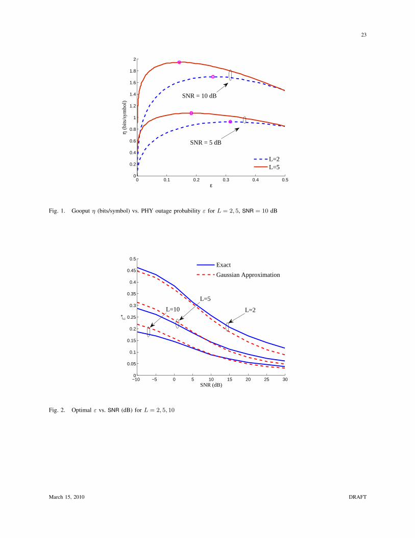
In order to provide a general understanding of ε⋆, Fig. 1 contains a plot of goodput η (numerically
computed) versus outage probability ε for L = 2 and L = 5 at SNR = 0 and 10 dB. For each curve, the
goodput-maximizing value of ε is circled. From this figure, we make the following observations:
• Making the physical layer too reliable or too unreliable yields poor goodput.
• The optimal outage probability decreases with SNR and L.
These turn out to be the key behaviors of the coding-ARQ tradeoff, and the remainder of this section is
devoted to analytically explain these behaviors through a Gaussian approximation.
Remark 1: Throughput the paper we consider the setting without channel state information at the
transmitter (CSIT). If there is CSIT, which generally is the case when the fading is slow relative to
the delay in the channel feedback loop, the optimization problem in Definition 1 turns out to be trivial.
When CSIT is available, the channel is essentially AWGN with an instantaneous SNR that is determined
2Note that in this definition we assume all possible code rates are possible; nonetheless, this formulation provides valuable
insight for systems in which the transmitter must choose from a finite set of code rates.3The expression for L = 1 is also derived in [2]. However, authors in [2] only consider L = 1 case rather than L > 1
scenarios, which are further investigated in our work.
March 15, 2010 DRAFT
6
by the fading realization but is known to the TX. If a capacity-achieving code with infinite codeword
block-length is used in the AWGN channel, the relationship between error and rate is a step-function:
ε =
0, if R < log2(1 + SNR|h|2
)(7a)
1, if R ≥ log2(1 + SNR|h|2
). (7b)
Thus, it is optimal to choose a rate very slightly below the instantaneous capacity log2(1 + SNR|h|2
).
For realistic codes with finite blocklength, the ε-R curve is not a step function but nonetheless is very
steep. For example, for turbo codes the waterfall characteristic of error vs. SNR curves (for fixed rate)
translates to a step-function-like error vs. rate curve for fixed SNR. Therefore, the transmitted rate should
be chosen close to the bottom of the step function.
A. Gaussian Approximation
The primary difficulty in finding ε⋆(SNR, L) stems from the fact that the outage probability in (2) can
only be expressed as an L-dimensional integral, except for the special case L = 1. To circumvent this
problem, we utilize a Gaussian approximation to the outage probability used in prior work [12]–[14].
The random variable 1L
∑Li=1 log2
(1 + SNR|hi|2
)is approximated by a N
(µ(SNR), σ2(SNR)/L
)random
variable, where µ(SNR) and σ2(SNR) are the mean and the variance of log2(1 + SNR|h|2
), respectively:
µ(SNR) = E|h|[log2(1 + SNR|h|2)
], (8)
σ2(SNR) = E|h|[log2(1 + SNR|h|2)
]2 − µ2(SNR). (9)
Closed forms for these quantities can be found in [15], [16]. Based on this approximation we have
ε ≈ Q
( √L
σ(SNR)(µ(SNR)−Rε)
), (10)
where Q(·) is the tail probability of a standard normal. Solving this equation for Rε and plugging into
(4) yields the following approximation for the goodput, which we denote as ηg:
ηg =
(µ(SNR)−Q−1(ε)
σ(SNR)√L
)(1− ε), (11)
where Q−1(ε) is the inverse of the Q function.
B. Optimization of Goodput Approximation
The optimization of ηg turns out to be more tractable. We first rewrite ηg as
ηg = µ(SNR)(1− κ ·Q−1(ε)
)(1− ε), (12)
March 15, 2010 DRAFT
7
where the constant κ ∈ (0, 1) is the µ-normalized standard deviation of the received mutual information:
κ , σ(SNR)
µ(SNR)√L. (13)
We can observe that κ decreases in SNR and L. We now define ε⋆g as the ηg-maximizing outage probability:
ε⋆g(SNR, L) , argmaxε
(1− κ ·Q−1(ε)
)(1− ε), (14)
where we have pulled out the constant µ(SNR) from (12) because it does not affect the maximization.
Proposition 1: The PHY reliability level that maximizes the Gaussian approximated goodput is the
unique solution to the following fixed point equation:(Q−1(ε⋆g)− (1− ε⋆g) ·
(Q−1(ε)
)′ |ε=ε⋆g
)−1= κ. (15)
Furthermore, ε⋆g is increasing in κ.
Proof: See Appendix A.
We immediately see that ε⋆g depends on the channel parameters only through κ. Furthermore, because
κ is decreasing in SNR and L, we see that ε⋆g decreases in L (i.e., the channel selectivity) and SNR.
Straightforward analysis shows that ε⋆g tends to zero as L increases approximately as 1/√L logL, while
ε⋆g tends to zero with SNR approximately as 1/√log SNR.
In Fig. 2, the exact optimal ε⋆ and the approximate-optimal ε⋆g are plotted vs. SNR (dB) for L = 2, 5,
and 10. The Gaussian approximation is seen to be reasonably accurate, and most importantly, correctly
captures behavior with respect to L and SNR.
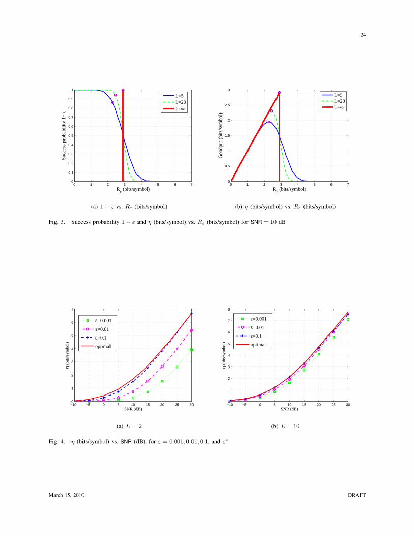
In order to gain an intuitive understanding of the optimization, in Fig. 3 the success probability 1− ε
(left) and the goodput η = Rε(1 − ε) (right) are plotted versus the transmitted rate R for SNR = 10
dB. For each L the goodput-maximizing operating point is circled. First consider the curves for L = 5.
For R up to approximately 1.5 bits/symbol the success probability is nearly one, i.e., ε ≈ 0. As a
result, the goodput η is approximately equal to R for R up to 1.5. When R is increased beyond 1.5
the success probability begins to decrease non-negligibly but the goodput nonetheless increases with R
because the increased transmission rate makes up for the loss in success probability (i.e., for the ARQ
re-transmissions). However, the goodput peaks at R = 2.3 because beyond this point the increase in
transmission rate no longer makes up for the increased re-transmissions; visually, the optimum rate (for
each value of L) corresponds to a point beyond which the success probability begins to drop off sharply
with the transmitted rate.
To understand the effect of the selectivity order L, notice that increasing L leads to a steepening
of the success probability-rate curve. This has the effect of moving the goodput curve closer to the
March 15, 2010 DRAFT
8
transmitted rate, which leads to a larger optimum rate and a larger optimum success probability (1− ε⋆).
To understand why ε⋆ decreases with SNR, based upon the rewritten version of ηg in (12) we see that the
governing relationship is between the success probability 1− ε and the normalized, rather than absolute,
transmission rate R/µ(SNR). Therefore, increasing SNR steepens the success probability-normalized rate
curve (similar to the effect of increasing L) and thus leads to a smaller value of ε⋆.
Is is important to notice that the optimum error probabilities in Fig. 2 are quite large, even for large
selectivity and at high SNR levels. This follows from the earlier explanation that decreasing the error
probability (and thus the rate) beyond a certain point is inefficient because the decrease in ARQ re-
transmissions does not make up for the loss in transmission rate.
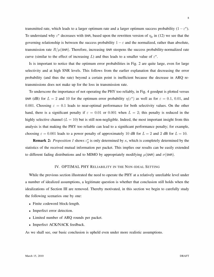
To underscore the importance of not operating the PHY too reliably, in Fig. 4 goodput is plotted versus
SNR (dB) for L = 2 and 10 for the optimum error probability η(ε⋆) as well as for ε = 0.1, 0.01, and
0.001. Choosing ε = 0.1 leads to near-optimal performance for both selectivity values. On the other
hand, there is a significant penalty if ε = 0.01 or 0.001 when L = 2; this penalty is reduced in the
highly selective channel (L = 10) but is still non-negligible. Indeed, the most important insight from this
analysis is that making the PHY too reliable can lead to a significant performance penalty; for example,
choosing ε = 0.001 leads to a power penalty of approximately 10 dB for L = 2 and 2 dB for L = 10.
Remark 2: Proposition 1 shows ε⋆g is only determined by κ, which is completely determined by the
statistics of the received mutual information per packet. This implies our results can be easily extended
to different fading distributions and to MIMO by appropriately modifying µ(SNR) and σ(SNR).
IV. OPTIMAL PHY RELIABILITY IN THE NON-IDEAL SETTING
While the previous section illustrated the need to operate the PHY at a relatively unreliable level under
a number of idealized assumptions, a legitimate question is whether that conclusion still holds when the
idealizations of Section III are removed. Thereby motivated, in this section we begin to carefully study
the following scenarios one by one:
• Finite codeword block-length.
• Imperfect error detection.
• Limited number of ARQ rounds per packet.
• Imperfect ACK/NACK feedback.
As we shall see, our basic conclusion is upheld even under more realistic assumptions.
March 15, 2010 DRAFT
9
A. Finite Codeword Block-length
Although in the previous section we assumed operation at the mutual information of infinite blocklength
codes, real systems must use finite blocklength codes. In order to determine the effect of finite blocklength
upon the optimal PHY reliability, we study the mutual information outage probability in terms of the
information spectrum, which captures the block error probability for finite blocklength codes. In [17], it
was shown that actual codes perform quite close to the information spectrum-based outage probability.
By extending the results of [17], [18], the outage probability with blocklength n (symbols) is
ε(n, SNR, L,R) = P
1
L
L∑i=1
log(1 + |hi|2SNR
)+
1
n
L∑i=1
√ |hi|2SNR
1 + |hi|2SNR·n/L∑j=1
ωij
≤ R
, (16)
where R is the transmitted rate in nats/symbol, and ωi,j’s are i.i.d. Laplace random variables [18], each
with zero mean and variance two. The first term in the sum is the standard infinite blocklength mutual
information expression, whereas the second term is due to the finite blocklength, and in particular captures
the effect of atypical noise realizations. This second term goes to zero as n → ∞ (i.e., atypical noise
does not occur in the infinite blocklength limit), but cannot be ignored for finite n.
The sum of i.i.d. Laplace random variables has a Bessel-K distribution, which is difficult to compute
for large n but can be very accurately approximated by a Gaussian as verified in [17]. Thus, the mutual
information conditioned on the L channel realizations is approximated by a Gaussian random variable:
N
(1
L
L∑i=1
log(1 + |hi|2SNR
),1
L
L∑i=1
2|hi|2SNR
n (1 + |hi|2SNR)
)(17)
(This is different from Section III-A, where the Gaussian approximation is made with respect to the
fading realizations). Therefore, we can approximate the outage probability with finite block-length n by
averaging the cumulative distribution function (CDF) of (17) over different channel realizations:
ε(n, SNR, L,R) ≈ E|h1|,...,|hL|Q
1L
∑Li=1 log
(1 + |hi|2SNR
)−R√
1L
∑Li=1
2|hi|2SNRn(1+|hi|2SNR)
. (18)
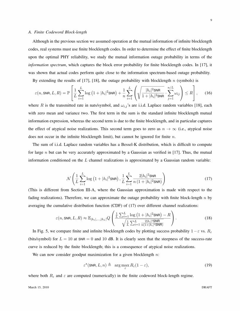
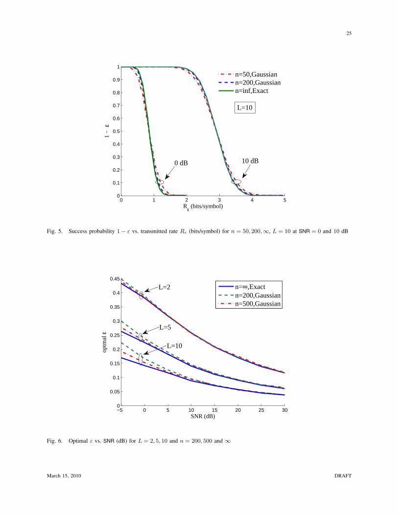
In Fig. 5, we compare finite and infinite blocklength codes by plotting success probability 1−ε vs. Rε
(bits/symbol) for L = 10 at SNR = 0 and 10 dB. It is clearly seen that the steepness of the success-rate
curve is reduced by the finite blocklength; this is a consequence of atypical noise realizations.
We can now consider goodput maximization for a given blocklength n:
ε⋆(SNR, L, n) , argmaxε
Rε(1− ε), (19)
where both Rε and ε are computed (numerically) in the finite codeword block-length regime.
March 15, 2010 DRAFT
10
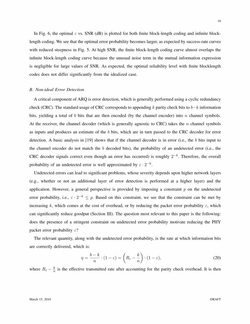
In Fig. 6, the optimal ε vs. SNR (dB) is plotted for both finite block-length coding and infinite block-
length coding. We see that the optimal error probability becomes larger, as expected by success-rate curves
with reduced steepness in Fig. 5. At high SNR, the finite block-length coding curve almost overlaps the
infinite block-length coding curve because the unusual noise term in the mutual information expression
is negligible for large values of SNR. As expected, the optimal reliability level with finite blocklength
codes does not differ significantly from the idealized case.
B. Non-ideal Error Detection
A critical component of ARQ is error detection, which is generally performed using a cyclic redundancy
check (CRC). The standard usage of CRC corresponds to appending k parity check bits to b−k information
bits, yielding a total of b bits that are then encoded (by the channel encoder) into n channel symbols.
At the receiver, the channel decoder (which is generally agnostic to CRC) takes the n channel symbols
as inputs and produces an estimate of the b bits, which are in turn passed to the CRC decoder for error
detection. A basic analysis in [19] shows that if the channel decoder is in error (i.e., the b bits input to
the channel encoder do not match the b decoded bits), the probability of an undetected error (i.e., the
CRC decoder signals correct even though an error has occurred) is roughly 2−k. Therefore, the overall
probability of an undetected error is well approximated by ε · 2−k.
Undetected errors can lead to significant problems, whose severity depends upon higher network layers
(e.g., whether or not an additional layer of error detection is performed at a higher layer) and the
application. However, a general perspective is provided by imposing a constraint p on the undetected
error probability, i.e., ε · 2−k ≤ p. Based on this constraint, we see that the constraint can be met by
increasing k, which comes at the cost of overhead, or by reducing the packet error probability ε, which
can significantly reduce goodput (Section III). The question most relevant to this paper is the following:
does the presence of a stringent constraint on undetected error probability motivate reducing the PHY
packet error probability ε?
The relevant quantity, along with the undetected error probability, is the rate at which information bits
are correctly delivered, which is:
η =b− k
n· (1− ε) =
(Rε −
k
n
)· (1− ε), (20)
where Rε − kn is the effective transmitted rate after accounting for the parity check overhead. It is then
March 15, 2010 DRAFT
11
relevant to maximize this rate subject to the constraint on undetected error:4:
(ε⋆, k⋆) , argmaxε,k
(Rε −
k
n
)· (1− ε) (21)
subject to ε · 2−k ≤ p
Although this optimization problem (nor the version based on the Gaussian approximation) is not
analytically tractable, it is easy to see that the solution corresponds to k⋆ = ⌈− log2(p/ε⋆)⌉, where ε⋆
is roughly the optimum packet error probability assuming perfect error detection (i.e. the solution from
Section III). In other words, the undetected error probability constraint should be satisfied by choosing
k sufficiently large while leaving the PHY transmitted rate nearly untouched. To better understand this,
note that reducing k by a bit requires reducing ε by a factor of two. The corresponding reduction in CRC
overhead is very small (roughly 1/n), while the reduction in the transmitted rate is much larger. Thus, if
we consider the choices of ε and k that achieve the constraint with equality, i.e., k = − log2(p/ε), goodput
decreases as ε is decreased below the packet error probability which is optimal under the assumption of
perfect error detection. In other words, operating the PHY at a more reliable point is not worth the small
reduction in CRC overhead.
C. End-to-End Delay Constraint
In certain applications such as Voice-over-IP (VoIP), there is a limit on the number of re-transmissions
per packet as well as a constraint on the fraction of packets that are not successfully delivered within
this limit. If such constraints are imposed, it may not be clear how aggressively ARQ should be utilized.
Consider a system where any packet that fails on its d-th attempt is discarded (i.e., at most d − 1
re-transmissions are allowed), but at most a fraction q of packets can be discarded, where q > 0 is a
reliability constraint. Under these conditions, the probability a packet is discarded is εd, i.e., the probability
of d consecutive decoding failures, while the long-term average rate at which packets are successfully
delivered still is Rε(1− ε). To understand why the goodput expression is unaffected by the delay limit,
note that the number of successfully delivered packets is equal to the number of transmissions in which
decoding is successful, regardless of which packets are transmitted in each slot. The delay constraint
only affects which packets are delivered in different slots, and thus does not affect the goodput.5
4For the sake of compactness, the dependence of ε⋆ and k⋆ upon SNR, L and n is suppressed henceforth, except where
explicit notation is required.5The goodput expression can alternatively be derived by computing the average number of ARQ rounds per packet (accounting
for the limit d), and then applying the renewal-reward theorem [20].
March 15, 2010 DRAFT
12
Since the discarded packet probability is εd, the reliability constraint requires ε ≤ q1/d. We can thus
consider maximization of goodput Rε(1 − ε) subject to the constraint ε ≤ q1/d. Because the goodput
is observed to be concave in ε, only two possibilities exist. If q1
d is larger than the optimal value of ε
for the unconstrained problem, then the optimal value of ε is unaffected by q. In the more interesting
and relevant case where q1
d is smaller than the optimal unconstrained ε, then goodput is maximized by
choosing ε equal to the upper bound q1
d .
Thus, a strict delay and reliability constraint forces the PHY to be more reliable than in the uncon-
strained case. However, amongst all allowed packet error probabilities, goodput is maximized by choosing
the largest. Thus, although strict constraints do not allow for very aggressive use of ARQ, nonetheless
ARQ should be utilized to the maximum extent possible.
D. Noisy ACK/NACK Feedback
We finally remove the assumption of perfect acknowledgements, and consider the realistic scenario
where ACK/NACK feedback is not perfect and where the acknowledgement overhead is factored in.
The main issue confronted here is the joint optimization of the reliability level of the forward data
channel and of the reverse acknowledgement (feedback/control) channel. As intuition suggests, reliable
communication is possible only if some combination of the forward and reverse reliability levels is
sufficiently large; thus, it is not clear if operating the PHY at a relatively unreliable level as suggested in
earlier sections is appropriate. The effects of acknowledgement errors can sometimes be reduced through
higher-layer mechanisms (e.g., sequence number check), but in order to shed the most light on the issue of
forward/reverse reliability, we focus on an extreme case where acknowledgement errors are most harmful.
In particular, we consider a setting with delay and reliability constraints as in Section IV-C, and where
any NACK to ACK error leads to a packet missing the delay deadline. We first describe the feedback
channel model, and then analyze performance.
1) Feedback Channel Model: We assume ACK/NACK feedback is performed over a Rayleigh fading
channel using a total of f symbols which are distributed on Lfb independently faded subchannels; here
Lfb is the diversity order of the feedback channel, which need not be equal to L, the forward channel
diversity order. Since the feedback is binary, BPSK is used with the symbol repeated on each sub-channel
f/Lfb times. For the sake of simplicity, we assume that the feedback channel has the same average SNR
as the forward channel, and that the fading on the feedback channel is independent of the fading on the
forward channel.
After maximum ratio combining at the receiver, the effective SNR is (f/Lfb) · SNR ·∑Lfb
i=1 |hi|2, where
March 15, 2010 DRAFT
13
h1, · · · , hLfb are the feedback channel fading coefficients. The resulting probability of error (denoted by
εfb), averaged over the fading realizations, is [21]:
εfb =
(1− ν
2
)Lfb
·Lfb−1∑j=0
(Lfb − 1 + j
j
)(1 + ν
2
)j
, (22)
where ν =√
(f/Lfb)·SNR1+(f/Lfb)·SNR . Clearly, εfb is decreasing in f and SNR.6
2) Performance Analysis: In order to analyze performance with non-ideal feedback, we must first
specify the rules by which the transmitter and receiver operate. The transmitter takes precisely the same
actions as in Section IV-C: the transmitter immediately moves on to the next packet whenever an ACK
is received, and after receiving d − 1 consecutive NACK’s (for a single packet) it attempts that packet
one last time but then moves on to the next packet regardless of the acknowledgement received for the
last attempt. Of course, the presence of feedback errors means that the received acknowledgement does
not always match the transmitted acknowledgement. The receiver also operates in the standard manner,
but we do assume that the receiver can always determine whether or not the packet being received is the
same as the packet received in the previous slot, as can be accomplished by a simple correlation; this
reasonable assumption is equivalent to the receiver having knowledge of acknowledgement errors.
In this setup an ACK→NACK error causes the transmitter to re-transmit the previous packet, instead
of moving on to the next packet. The receiver is able to recognize that an acknowledgement error has
occurred (through correlation of the current and previous received packets), and because it already decoded
the packet correctly it does not attempt to decode again. Instead, it simply transmits an ACK once again.
Thus, each ACK→NACK error has the relatively benign effect of wasting one ARQ round.
On the other hand, NACK→ACK errors have a considerably more deleterious effect because upon
reception of an ACK, the transmitter automatically moves on to the next packet. Because we are
considering a stringent delay constraint, we assume that such a NACK→ACK error cannot be recovered
from and thus we consider it as a lost packet that is counted towards the reliability constraint. This is, in
some sense, a worst-case assumption that accentuates the effect of NACK→ACK errors; some comments
related to this point are put forth at the end of this section.
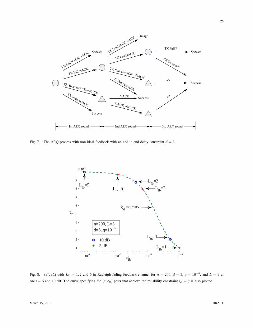
To more clearly illustrate the model, the complete ARQ process is shown in Fig. 7 for d = 3. Each
branch is labeled with the success/failure of the transmission as well as the acknowledgement (including
errors). Circle nodes refer to states in which the receiver has yet to successfully decode the packet, whereas
6Asymmetric decision regions can be used, in which case 0 → 1 and 1 → 0 errors have unequal probabilities. However, this
does not significantly affect performance and thus is not considered.
March 15, 2010 DRAFT
14
triangles refer to states in which the receiver has decoded correctly. A packet loss occurs if there is a
decoding failure followed by a NACK→ACK error in the first two rounds, or if decoding fails in all three
attempts. All other outcomes correspond to cases where the receiver is able to decode the packet in some
round, and thus successful delivery of the packet. In these cases, however, the number of ARQ rounds
depends on the first time at which the receiver can decode and when the ACK is correctly delivered. (If
an ACK is not successfully delivered, it may take up to d rounds before the transmitter moves on to the
next packet.) Notice that after the d-th attempt, the transmitter moves on to the next packet regardless of
what acknowledgement is received; this is due to the delay constraint that the transmitter follows.
Based on the figure and the independence of decoding and feedback errors across rounds, the probability
that a packet is lost (i.e., it is not successfully delivered within d rounds) is:
ξd = ε · εfb + ε2(1− εfb)εfb + · · ·+ εd−1(1− εfb)d−2εfb + εd(1− εfb)
d−1, (23)
where the first d−1 terms represent decoding failures followed by a NACK→ACK error (more specifically,
the l-th term corresponds to l− 1 decoding failures and l− 1 correct NACK transmissions, followed by
another decoding failure and a NACK→ACK error), and the last term is the probability of d decoding
failures and d− 1 correct NACK transmissions. If we alternatively compute the success probability, we
get the following different expression for ξd:
ξd = 1−d∑
i=1
(1− ε) · εi−1 · (1− εfb)i−1, (24)
where the i-th summand is the probability that successful forward transmission occurs in the i-th ARQ
round. Based upon (23) and (24) we see that ξd is increasing in both ε and εfb. Thus, a desired packet
loss probability ξd can be achieved by different combinations of the forward channel reliability and the
feedback channel reliability: a less reliable forward channel requires a more reliable feedback channel,
and vice versa.
As in Section IV-C we impose a reliability constraint ξd ≤ q, which by (23) translates to a joint
constraint on ε and εfb. The relatively complicated joint constraint can be accurately approximated by
two much simpler constraints. Since we must satisfy ε ≤ q1
d even with perfect feedback (εfb = 0), for
any εfb > 0 we also must satisfy ε ≤ q1
d (this ensures that d consecutive decoding failures do not occur
too frequently). Furthermore, by examining (23) it is evident that the first term is dominant in the packet
loss probability expression. Thus the constraint ξd ≤ q essentially translates to the simplified constraints
ε · εfb ≤ q and ε ≤ q1
d . (25)
March 15, 2010 DRAFT
15
These simplified constraints are very accurate for values of ε not too close to q1
d . On the other hand, as
ε approaches q1
d , εfb must go to zero very rapidly (i.e. much faster than q/ε) in order for ξd ≤ q.
The first constraint in (25) reveals a general design principle: the combination of the forward and
feedback channel must be sufficiently reliable. This is because ε · εfb is precisely the probability that a
packet is lost because the initial transmission is decoded incorrectly and is followed by a NACK→ACK
error.
Having established the reliability constraint, we now proceed to maximizing goodput while taking
acknowledgement errors and ARQ overhead into account. With respect to the long-term average goodput,
by applying the renewal-reward theorem again we obtain:
η =n
n+ f· Rε(1− ξd)
E[X]. (26)
where random variable X is the number of ARQ rounds per packet, and E[X] is derived in Appendix
B. Here, nn+f is the feedback overhead penalty because each packet spanning n symbols is followed by
f symbols to convey the acknowledgement.
We now maximize goodput with respect to both the forward and feedback channel error probabilities:
(ε⋆, ε⋆fb) , argmaxε,εfb
n
n+ f· Rε(1− ξd)
E[X](27)
subject to ξd ≤ q
noting that εfb is a decreasing function of the number of feedback symbols f , according to (22). This
optimization is not analytically tractable, but can be easily solved numerically and can be understood
through examination of the dominant relationships. The overhead factor n/(n+ f) clearly depends only
on εfb (i.e., f ). Although the second term Rε(1− ξd)/E[X] depends on both ε and εfb, the dependence
upon εfb is relatively minor as long as εfb is reasonably small (i.e. less than 10%). Thus, it is reasonable
to consider the perfect feedback setting, in which case the second term is Rε(1 − ε). Therefore, the
challenge is balancing the feedback channel overhead factor nn+f with the efficiency of the forward
channel, approximately Rε(1 − ε), while satisfying the constraint in (25). If f is chosen small, the
feedback errors must be compensated with a very reliable, and thus inefficient, forward channel; on the
other hand, choosing f large incurs a large feedback overhead penalty but allows for a less reliable, and
thus more efficient, forward channel.
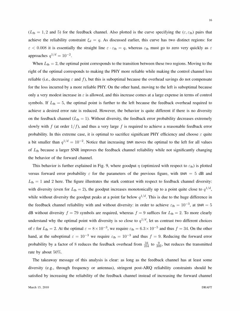
In Fig. 8, the jointly optimal (ε⋆, ε⋆fb) are plotted for a conservative set of forward channel parameters
(L = 3 with SNR = 5 or 10 dB, and n = 200 data symbols per packet), stringent delay and reliability
constraints (up to d = 3 ARQ rounds and a reliability constraint q = 10−6), and different diversity orders
March 15, 2010 DRAFT
16
(Lfb = 1, 2 and 5) for the feedback channel. Also plotted is the curve specifying the (ε, εfb) pairs that
achieve the reliability constraint ξd = q. As discussed earlier, this curve has two distinct regions: for
ε < 0.008 it is essentially the straight line ε · εfb = q, whereas εfb must go to zero very quickly as ε
approaches q1/d = 10−2.
When Lfb = 2, the optimal point corresponds to the transition between these two regions. Moving to the
right of the optimal corresponds to making the PHY more reliable while making the control channel less
reliable (i.e., decreasing ε and f ), but this is suboptimal because the overhead savings do not compensate
for the loss incurred by a more reliable PHY. On the other hand, moving to the left is suboptimal because
only a very modest increase in ε is allowed, and this increase comes at a large expense in terms of control
symbols. If Lfb = 5, the optimal point is further to the left because the feedback overhead required to
achieve a desired error rate is reduced. However, the behavior is quite different if there is no diversity
on the feedback channel (Lfb = 1). Without diversity, the feedback error probability decreases extremely
slowly with f (at order 1/f ), and thus a very large f is required to achieve a reasonable feedback error
probability. In this extreme case, it is optimal to sacrifice significant PHY efficiency and choose ε quite
a bit smaller than q1/d = 10−2. Notice that increasing SNR moves the optimal to the left for all values
of Lfb because a larger SNR improves the feedback channel reliability while not significantly changing
the behavior of the forward channel.
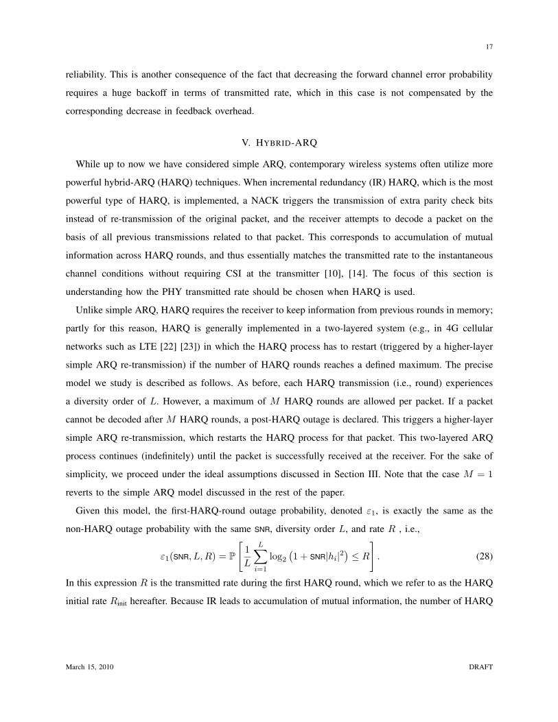
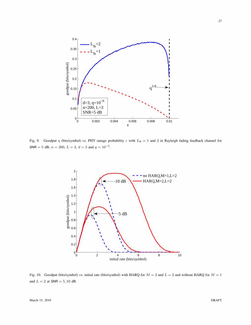
This behavior is further explained in Fig. 9, where goodput η (optimized with respect to εfb) is plotted
versus forward error probability ε for the parameters of the previous figure, with SNR = 5 dB and
Lfb = 1 and 2 here. The figure illustrates the stark contrast with respect to feedback channel diversity:
with diversity (even for Lfb = 2), the goodput increases monotonically up to a point quite close to q1/d,
while without diversity the goodput peaks at a point far below q1/d. This is due to the huge difference in
the feedback channel reliability with and without diversity: in order to achieve εfb = 10−3, at SNR = 5
dB without diversity f = 79 symbols are required, whereas f = 9 suffices for Lfb = 2. To more clearly
understand why the optimal point with diversity is so close to q1/d, let us contrast two different choices
of ε for Lfb = 2. At the optimal ε = 8×10⁻³, we require εfb = 6.3×10⁻⁵ and thus f = 34. On the other
hand, at the suboptimal ε = 10−3 we require εfb = 10−3 and thus f = 9. Reducing the forward error
probability by a factor of 8 reduces the feedback overhead from 34234 to 9
209 , but reduces the transmitted
rate by about 50%.
The takeaway message of this analysis is clear: as long as the feedback channel has at least some
diversity (e.g., through frequency or antennas), stringent post-ARQ reliability constraints should be
satisfied by increasing the reliability of the feedback channel instead of increasing the forward channel
March 15, 2010 DRAFT
17
reliability. This is another consequence of the fact that decreasing the forward channel error probability
requires a huge backoff in terms of transmitted rate, which in this case is not compensated by the
corresponding decrease in feedback overhead.
V. HYBRID-ARQ
While up to now we have considered simple ARQ, contemporary wireless systems often utilize more
powerful hybrid-ARQ (HARQ) techniques. When incremental redundancy (IR) HARQ, which is the most
powerful type of HARQ, is implemented, a NACK triggers the transmission of extra parity check bits
instead of re-transmission of the original packet, and the receiver attempts to decode a packet on the
basis of all previous transmissions related to that packet. This corresponds to accumulation of mutual
information across HARQ rounds, and thus essentially matches the transmitted rate to the instantaneous
channel conditions without requiring CSI at the transmitter [10], [14]. The focus of this section is
understanding how the PHY transmitted rate should be chosen when HARQ is used.
Unlike simple ARQ, HARQ requires the receiver to keep information from previous rounds in memory;
partly for this reason, HARQ is generally implemented in a two-layered system (e.g., in 4G cellular
networks such as LTE [22] [23]) in which the HARQ process has to restart (triggered by a higher-layer
simple ARQ re-transmission) if the number of HARQ rounds reaches a defined maximum. The precise
model we study is described as follows. As before, each HARQ transmission (i.e., round) experiences
a diversity order of L. However, a maximum of M HARQ rounds are allowed per packet. If a packet
cannot be decoded after M HARQ rounds, a post-HARQ outage is declared. This triggers a higher-layer
simple ARQ re-transmission, which restarts the HARQ process for that packet. This two-layered ARQ
process continues (indefinitely) until the packet is successfully received at the receiver. For the sake of
simplicity, we proceed under the ideal assumptions discussed in Section III. Note that the case M = 1
reverts to the simple ARQ model discussed in the rest of the paper.
Given this model, the first-HARQ-round outage probability, denoted ε1, is exactly the same as the
non-HARQ outage probability with the same SNR, diversity order L, and rate R , i.e.,
ε1(SNR, L,R) = P
[1
L
L∑i=1
log2(1 + SNR|hi|2
)≤ R
]. (28)
In this expression R is the transmitted rate during the first HARQ round, which we refer to as the HARQ
initial rate Rinit hereafter. Because IR leads to accumulation of mutual information, the number of HARQ
March 15, 2010 DRAFT
18
rounds needed to decode a packet is the smallest integer T (1 ≤ T ≤ M ) such that
T∑i=1
1
L
L∑j=1
log2(1 + SNR|hi,j |2
) > Rinit. (29)
Therefore, the post-HARQ outage, denoted by ε, is:
ε(SNR, L,M,Rinit) = P
M∑i=1
1
L
L∑j=1
log2(1 + SNR|hi,j |2
) ≤ Rinit
. (30)
This is the probability that a packet fails to be decoded after M HARQ rounds, and thus is the probability
that the HARQ process has to be restarted.
Using the renewal-reward theorem as in [10] yields the following expression for the long-term average
goodput with HARQ:
η =Rinit(1− ε)
E[T ], (31)
where the distribution of T is determined by (29). Our interest is in finding the initial rate Rinit that
maximizes η. This optimization is not analytically tractable, but we can nonetheless provide some insight.
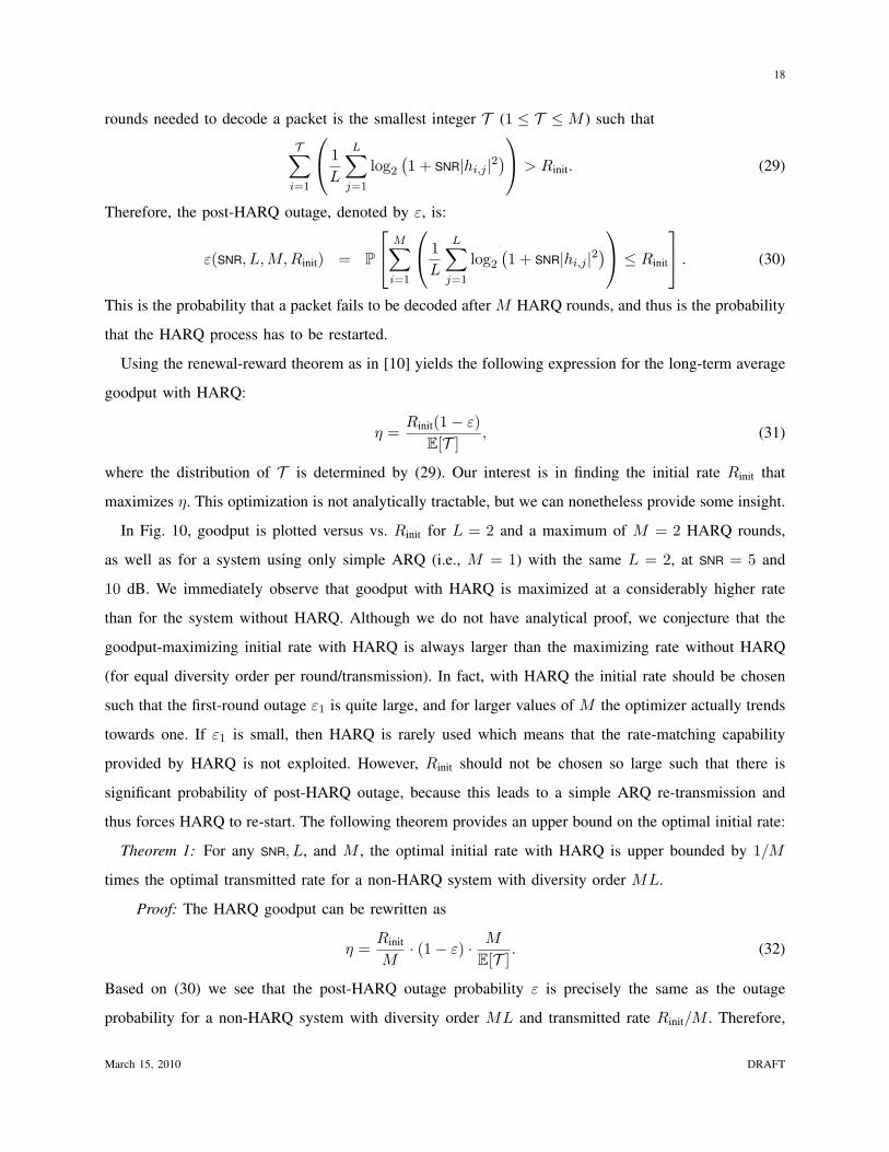
In Fig. 10, goodput is plotted versus vs. Rinit for L = 2 and a maximum of M = 2 HARQ rounds,
as well as for a system using only simple ARQ (i.e., M = 1) with the same L = 2, at SNR = 5 and
10 dB. We immediately observe that goodput with HARQ is maximized at a considerably higher rate
than for the system without HARQ. Although we do not have analytical proof, we conjecture that the
goodput-maximizing initial rate with HARQ is always larger than the maximizing rate without HARQ
(for equal diversity order per round/transmission). In fact, with HARQ the initial rate should be chosen
such that the first-round outage ε1 is quite large, and for larger values of M the optimizer actually trends
towards one. If ε1 is small, then HARQ is rarely used which means that the rate-matching capability
provided by HARQ is not exploited. However, Rinit should not be chosen so large such that there is
significant probability of post-HARQ outage, because this leads to a simple ARQ re-transmission and
thus forces HARQ to re-start. The following theorem provides an upper bound on the optimal initial rate:
Theorem 1: For any SNR, L, and M , the optimal initial rate with HARQ is upper bounded by 1/M
times the optimal transmitted rate for a non-HARQ system with diversity order ML.
Proof: The HARQ goodput can be rewritten as
η =Rinit
M· (1− ε) · M
E[T ]. (32)
Based on (30) we see that the post-HARQ outage probability ε is precisely the same as the outage
probability for a non-HARQ system with diversity order ML and transmitted rate Rinit/M . Therefore,
March 15, 2010 DRAFT
19
the term (Rinit/M)(1− ε) in (32) is precisely the goodput for a non-HARQ system with diversity order
ML. Based on (29) we can see that the term M/E[T ] is decreasing in Rinit/M , and thus the value of
Rinit/M that maximizes (32) is smaller than the value that maximizes (Rinit/M)(1− ε).
Notice that ML is the maximum diversity experienced by a packet if HARQ is used, whereas ML is
the precise diversity order experienced by each packet in the reference system (in the theorem) without
HARQ. Combined with our earlier observation, we see that the initial rate should be chosen large enough
such that HARQ is sufficiently utilized, but not so large such that simple ARQ is overly used.
VI. CONCLUSION
In this paper we have conducted a detailed study of the optimum physical layer reliability when
simple ARQ is used to re-transmit incorrectly decoded packets. Our findings show that when a cross-
layer perspective is taken, it is optimal to use a rather unreliable physical layer (e.g., a packet error
probability of 10% for a wide range of channel parameters). The fundamental reason for this is that
making the physical layer very reliable requires a very conservative transmitted rate in a fading channel
(without instantaneous channel knowledge at the transmitter).
Our findings are quite general, in the sense that the PHY should not be operated reliably even in
scenarios in which intuition might suggest PHY-level reliability is necessary. For example, if a smaller
packet error mis-detection probability is desired, it is much more efficient to utilize additional error
detection bits (e.g., CRC) as compared to performing additional error correction (i.e., making the PHY
more reliable). A delay constraint imposes an upper bound on the number of ARQ re-transmissions and
an upper limit on the PHY error probability, but an optimized system should operate at exactly this
level and no lower. Finally, when acknowledgement errors are taken into account and high end-to-end
reliability is required, such reliability should be achieved by designing a reliable feedback channel instead
of a reliable data (PHY) channel.
In a broader context, one important message is that traditional diversity metrics, which characterize
how quickly the probability of error can be made very small, may no longer be appropriate for wireless
systems due to the presence of ARQ. As seen in [24] in the context of multi-antenna communication,
this change can significantly reduce the attractiveness of transmit diversity techniques that reduce error
at the expense of rate.
March 15, 2010 DRAFT
20
APPENDIX A
PROOF OF PROPOSITION 1
We first prove the strict concavity of ηg. For any invertible function f(·), the following holds [25]:(f−1(a)
)′=
1
f ′(f−1(a)). (33)
By combining this with Q(x) =∫∞x
1√2πe−
t2
2 dt, we get(Q−1(ε)
)′= −
√2πe
(Q−1(ε))2
2 , (34)
which is strictly negative. According to this, the second derivative of ηg(ε) is:
(ηg(ε))′′ = κµ
(Q−1(ε)
)′ (2 + (1− ε)
√2πe
(Q−1(ε))2
2 Q−1(ε)). (35)
Because κ(Q−1(ε)
)′< 0, in order to prove (ηg(ε))
′′ < 0 we only need to show that the expression
inside the parenthesis in (35) is strictly positive. If we substitute ε = Q(x) (here we define x = Q−1(ε))
, then we only need to prove (Q(x)− 1)ex2
2 x <√
2π . Notice when x ≥ 0, the left hand side is negative
(because Q(x) ≤ 1) and the inequality holds. When x < 0, the left hand side becomes Q(−x)ex2
2 (−x).
From [26], Q(−x) < 1√2π(−x)
e−x2
2 , so if x < 0,
(Q(x)− 1)ex2
2 x <1√
2π(−x)e−
x2
2 ex2
2 (−x) =1√2π
<
√2
π. (36)
As a result, the second derivative of ηg(ε) is strictly smaller than zero and thus ηg is strictly concave in
ε. Since ηg is strictly concave in ε, we reach the fixed point equation in (15) by setting the first derivative
to zero. The concavity of ηg implies (ηg(ε))′ is decreasing in ε, and thus from (15) we see that ε⋆g is
increasing in κ.
APPENDIX B
EXPECTED ARQ ROUNDS WITH ACKNOWLEDGEMENT ERRORS
If the ARQ process terminates after i rounds (1 ≤ i ≤ d− 1), the reasons for that can be:
• The first i decoding attempts are unsuccessful, the first i − 1 NACKs are received correctly, but a
NACK→ACK error happens in the i-th round, the probability of which is εi · (1− εfb)i−1 · εfb.
• The packet is decoded correctly in the j-th round (for 1 ≤ j ≤ i), but the ACK is not correctly
received until the i-th round. This corresponds to j− 1 decoding failures with correct acknowledge-
ments, followed by a decoding success and i− j acknowledgement errors (ACK→NACK), and then
a correct acknowledgement:∑i
j=1 εj−1(1− εfb)
j(1− ε)εi−jfb .
March 15, 2010 DRAFT
21
These events are all exclusive, and thus we can sum the above probabilities. For X = d, we notice that
the ARQ process takes the maximum of d rounds if:
• There are d decoding failures with d−1 correct NACKs, the probability of which is εd−1·(1−εfb)d−1.
• The packet is decoded correctly in the j-th round (for 1 ≤ j ≤ d−1), but the ACK is never received
correctly. This corresponds to j − 1 decoding failures with correct NACKs, followed by a decoding
success and d− j acknowledgement errors (ACK→NACK):∑d−1
j=1 εj−1(1− εfb)
j−1(1− ε)εd−jfb .
These events are again exclusive. Therefore, the expected number of rounds is:
E[X] =
d−1∑i=1
i ·
εi · (1− εfb)i−1 · εfb +
i∑j=1
εj−1(1− εfb)j(1− ε)εi−j
fb
+d ·
εd−1 · (1− εfb)d−1 +
d−1∑j=1
εj−1(1− εfb)j−1(1− ε)εd−j
fb
. (37)
REFERENCES
[1] M. Luby, T. Gasiba, T. Stockhammer, and M. Watson, “Reliable multimedia download delivery in cellular broadcast
networks,” IEEE Trans. Broadcasting, vol. 53, no. 1 Part 2, pp. 235–246, 2007.
[2] C. Berger, S. Zhou, Y. Wen, P. Willett, and K. Pattipati, “Optimizing joint erasure-and error-correction coding for wireless
packet transmissions,” IEEE Transactions on Wireless Communications, vol. 7, no. 11 Part 2, pp. 4586–4595, 2008.
[3] T. A. Courtade and R. D. Wesel, “A cross-layer perspective on rateless coding for wireless channels,” Proc. of IEEE Int’l
Conf. in Commun. (ICC’09), pp. 1–6, Jun. 2009.
[4] X. Chen, V. Subramanian, and D. J. Leith., “PHY modulation/rate control for fountain codes in 802.11 WLANs,” submitted
to IEEE Trans. Wireless Comm., June 2009.
[5] G. Carie, G. Taricco, and E. Biglieri, “Optimum power control over fading channels,” IEEE Trans. Inform. Theory, vol. 45,
no. 5, pp. 1468–1489, Jul. 1999.
[6] A. Guillen i Fabregas and G. Caire, “Coded modulation in the block-fading channel: coding theorems and code
construction,” IEEE Trans. Inf. Theory, vol. 52, no. 1, pp. 91–114, Jan. 2006.
[7] N. Prasad and M. K. Varanasi, “Outage theorems for MIMO block-fading channels,” IEEE Trans. Inform. Theory, vol. 52,
no. 12, pp. 5284–5296, Dec. 2006.
[8] E. Malkamaki and H. Leib, “Coded diversity on block-fading channels,” IEEE Trans. Inf. Theory, vol. 45, no. 2, pp.
771–781, Mar. 1999.
[9] D. Tse and P. Viswanath, Fundamentals of Wireless Communications. Cambridge University, 2005.
[10] G. Caire and D. Tuninetti, “The throughput of hybrid-ARQ protocols for the Gaussian collision channel,” IEEE Trans.
Inform. Theory, vol. 47, no. 4, pp. 1971–1988, Jul. 2001.
[11] R. Corless, G. Gonnet, D. Hare, D. Jeffrey, and D. Knuth, “On the LambertW function,” Advances in Computational
Mathematics, vol. 5, no. 1, pp. 329–359, 1996.
[12] P. J. Smith and M. Shafi, “On a Gaussian approximation to the capacity of wireless MIMO systems,” Proc. of IEEE Int’l
Conf. in Commun. (ICC’02), pp. 406–410, Apr. 2002.
March 15, 2010 DRAFT
22
[13] G. Barriac and U. Madhow, “Characterizing outage rates for space-time communication over wideband channels,” IEEE
Trans. Commun., vol. 52, no. 4, pp. 2198–2207, Dec. 2004.
[14] P. Wu and N. Jindal, “Performance of hybrid-ARQ in block-fading channels: a fixed outage probability analysis,” to appear
at IEEE Trans. Commun., vol. 58, no. 4, Apr. 2010.
[15] M. S. Alouini and A. J. Goldsmith, “Capacity of Rayleigh fading channels under different adaptive transmission and
diversity-combining techniques,” IEEE Trans. Veh. Technol., vol. 48, no. 4, pp. 1165–1181, Jul. 1999.
[16] M. R. McKay, P. J. Smith, H. A. Suraweera, and I. B. Collings, “On the mutual information distribution of OFDM-based
spatial multiplexing: exact variance and outage approximation,” IEEE Trans. Inform. Theory, vol. 54, no. 7, pp. 3260–3278,
Jul. 2008.
[17] D. Buckingham and M. Valenti, “The information-outage probability of finite-length codes over AWGN channels,” 42nd
Annunal Conf. Inform. Sciences and Systems (CISS’08), pp. 390–395, 2008.
[18] J. Laneman, “On the distribution of mutual information,” Proc. Workshop on Information Theory and its Applications
(ITA’06), 2006.
[19] H. E. Gamal, G. Caire, and M. E. Damen, “The MIMO ARQ channel: diversity-multiplexing-delay tradeoff,” IEEE Trans.
Inform. Theory, vol. 52, no. 8, pp. 3601–3621, Aug. 2006.
[20] R. Wolff, Stochastic Modeling and the Theory of Queues. Prentice hall, 1989.
[21] A. Goldsmith, Wireless Communications. Cambridge University Press, 2005.
[22] M. Meyer, H. Wiemann, M. Renfors, J. Torsner, and J. Cheng, “ARQ concept for the UMTS Long-Term Evolution,” IEEE
64th Vehicular Technology Conference (VTC’06), pp. 1–5, Sep. 2006.
[23] H. Ekstrom, A. Furuskar, J. Karlsson, M. Meyer, S. Parkvall, J. Torsner, and M. Wahlqvist, “Technical solutions for the
3G long-term evolution,” IEEE Communications Magazine, vol. 44, no. 3, pp. 38–45, 2006.
[24] A. Lozano and N. Jindal, “Transmit diversity v. spatial multiplexing in modern MIMO systems,” IEEE Trans. Wireless
Commun., vol. 9, no. 1, pp. 186–197, Jan. 2010.
[25] T. Apostol, Mathematical Analysis. Addison-Wesley Reading, MA, 1974.
[26] N. Kingsbury, “Approximation formula for the Gaussian error integral, Q(x),” http://cnx.org/content/m11067/latest/.
March 15, 2010 DRAFT
23
0 0.1 0.2 0.3 0.4 0.50
0.2
0.4
0.6
0.8
1
1.2
1.4
1.6
1.8
2
η (b
its/s
ymbo
l)
ε
L=2L=5
SNR = 10 dB
SNR = 5 dB
Fig. 1. Gooput η (bits/symbol) vs. PHY outage probability ε for L = 2, 5, SNR = 10 dB
−10 −5 0 5 10 15 20 25 300
0.05
0.1
0.15
0.2
0.25
0.3
0.35
0.4
0.45
0.5
SNR (dB)
ε?
Exact
Gaussian Approximation
L=10
L=5
L=2
Fig. 2. Optimal ε vs. SNR (dB) for L = 2, 5, 10
March 15, 2010 DRAFT
24
0 1 2 3 4 5 6 70
0.1
0.2
0.3
0.4
0.5
0.6
0.7
0.8
0.9
1
Rε (bits/symbol)
Suc
cess
pro
babi
lity
1−
ε
L=5L=20L=∞
(a) 1− ε vs. Rε (bits/symbol)
0 1 2 3 4 5 6 70
0.5
1
1.5
2
2.5
3
Rε (bits/symbol)
Goo
dput
(bi
ts/s
ymbo
l)
L=5L=20L=∞
(b) η (bits/symbol) vs. Rε (bits/symbol)
Fig. 3. Success probability 1− ε and η (bits/symbol) vs. Rε (bits/symbol) for SNR = 10 dB
−10 −5 0 5 10 15 20 25 300
1
2
3
4
5
6
7
SNR (dB)
η (b
its/s
ymbo
l)
ε=0.001
ε=0.01
ε=0.1
optimal
(a) L = 2
−10 −5 0 5 10 15 20 25 300
1
2
3
4
5
6
7
8
SNR (dB)
η (b
its/s
ymbo
l)
ε=0.001
ε=0.01
ε=0.1
optimal
(b) L = 10
Fig. 4. η (bits/symbol) vs. SNR (dB), for ε = 0.001, 0.01, 0.1, and ε⋆
March 15, 2010 DRAFT
25
0 1 2 3 4 50
0.1
0.2
0.3
0.4
0.5
0.6
0.7
0.8
0.9
1
Rε (bits/symbol)
1 −
ε
n=50,Gaussiann=200,Gaussiann=inf,Exact
L=10
0 dB 10 dB
Fig. 5. Success probability 1− ε vs. transmitted rate Rε (bits/symbol) for n = 50, 200,∞, L = 10 at SNR = 0 and 10 dB
−5 0 5 10 15 20 25 300
0.05
0.1
0.15
0.2
0.25
0.3
0.35
0.4
0.45
SNR (dB)
optm
al ε
n=∞,Exactn=200,Gaussiann=500,Gaussian
L=2
L=10
L=5
Fig. 6. Optimal ε vs. SNR (dB) for L = 2, 5, 10 and n = 200, 500 and ∞
March 15, 2010 DRAFT
26
Fig. 7. The ARQ process with non-ideal feedback with an end-to-end delay constraint d = 3.
10−6
10−5
10−4
10−3
1
2
3
4
5
6
7
8
9
x 10−3
ε?
fb
ε?
10 dB5 dB
Lfb
=2
Lfb
=2L
fb=5
Lfb
=5
Lfb
=1
n=200, L=3d=3, q=10−6
ξd =q curve
Lfb
=1
Fig. 8. (ε⋆, ε⋆fb) with Lfb = 1, 2 and 5 in Rayleigh fading feedback channel for n = 200, d = 3, q = 10−6, and L = 3 at
SNR = 5 and 10 dB. The curve specifying the (ε, εfb) pairs that achieve the reliability constraint ξd = q is also plotted.
March 15, 2010 DRAFT
27
0 0.002 0.004 0.006 0.008 0.010
0.05
0.1
0.15
0.2
0.25
0.3
0.35
0.4
ε
good
put (
bits
/sym
bol)
Lfb
=2
Lfb
=1
d=3, q=10−6
n=200, L=3SNR=5 dB
q1/d
Fig. 9. Goodput η (bits/symbol) vs. PHY outage probability ε with Lfb = 1 and 2 in Rayleigh fading feedback channel for
SNR = 5 dB, n = 200, L = 3, d = 3 and q = 10−6.
0 2 4 6 8 100
0.2
0.4
0.6
0.8
1
1.2
1.4
1.6
1.8
2
initial rate (bits/symbol)
good
put (
bits
/sym
bol)
no HARQ,M=1,L=2HARQ,M=2,L=2
5 dB
10 dB
Fig. 10. Goodput (bits/symbol) vs. initial rate (bits/symbol) with HARQ for M = 2 and L = 2 and without HARQ for M = 1
and L = 2 at SNR = 5, 10 dB.
March 15, 2010 DRAFT