�

�

�

�

Signal Processing Methods for NetworkAnomaly Detection

Lingsong Zhang

Department of Statistics and Operations Research

Email: LSZHANG@email.unc.edu

March 7, 2005; March 9, 2005

1

�

�

�

�

Outline

• Introduction and Background

• Single Time Series Methods

– Spectral Analysis

– Wavelet Analysis

– Singular Value Decomposition

• Multiple Time Series and Multivariate Methods

– Multivariate Outlier Detection

– Principal Component Analysis

• Further Work and Comments

2

�

�

�

�

Part I – Introduction

3

�

�

�

�

Introduction and Background

• DoS is popular now, with possible catastrophe, by consumingfinite resource

• Detection of and response to DoS is essential for network

• Network Traffic itself is hard to be analyze

– Non-Gaussian, Non-Stationary, Long Range Dependence,Heavy tailed

• Attackers will try to make the attack traffic hard to bedistinguished from normal traffic

• Not sure which measurements best fit for anomalies detection

• Not sure which method is best

4

�

�

�

�

Major issues for Detection

• Stand-alone intrusion detection appliances shouldautomatically recognize the network is under attack and adjustits traffic flow to ease the attack impact downstream

• The detection and response techniques should be adaptable toa wide range of network environments, without significantmanual tuning

• False negative and false positive should be as small as possible

• Attack response should employ intelligent packet discardmechanisms to reduce the downstream impact of the floodwhile preserving and routing the non-attack packets

• The detection method should be effective against a variety ofattack tools available today and also robust against futureattempts by attackers to evade detection

5

�

�

�

�

Part II – Analysis Methods

6

�

�

�

�

Analysis Methods

• Single Time Series Analysis Methods

– Spectral analysis

– Wavelet analysis

– Singular Value Decomposition

– other methods?

• Multiple Time Series or Multivariate Analysis Methods

– Multivariate Outlier Detection Method

– Principal Component analysis (Singular ValueDecomposition) Method

7

�

�

�

�

Spectral analysis in Defense Against DoS Attacks

• Motivation

– normal TCP flows must exhibit periodicity in packettransport associated with round-trip times.

– fourier transform is a good tool to test the periodicity.

• Spectral Analysis

– Fourier transform is a frequency-domain representation of afunction. This allows us to examine the function fromanother point of view, the transformed (frequency) domain.

– A good referenceBrigham, E. Oran, (1988) “The fast Fourier transform andits applications”, Prentice-Hall, Inc.

8

�

�

�

�

Outline of Spectral Analysis

• An simple example

• Properties of TCP traffic

– Simulated traffic

– Real traffic

• Discussion

9

�

�

�

�

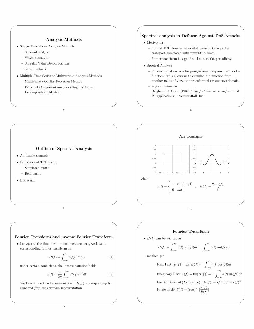
An example

−2 −1.5 −1 −0.5 0 0.5 1 1.5 2−1

−0.5

0

0.5

1

1.5

2

t

h(t)

−10 −5 0 5 10−1

−0.5

0

0.5

1

1.5

2

f

H(f

)

where

h(t) =

⎧⎨⎩

1 t ∈ [−1, 1]

0 o.w., H(f) =

2sin(f)f

10

�

�

�

�

Fourier Transform and inverse Fourier Transform

• Let h(t) as the time series of one measurement, we have acorresponding fourier transform as

H(f) =∫ ∞

−∞h(t)e−iftdt (1)

under certain conditions, the inverse equation holds

h(t) =12π

∫ ∞

−∞H(f)eitfdf (2)

We have a bijection between h(t) and H(f), corresponding totime and frequency domain representation

11

�

�

�

�

Fourier Transform

• H(f) can be written as

H(f) =∫ ∞

−∞h(t) cos(ft)dt − i

∫ ∞

−∞h(t) sin(ft)dt

we then get

Real Part: R(f) = Re(H(f)) =∫ ∞

−∞h(t) cos(ft)dt

Imaginary Part: I(f) = Im(H(f)) = −∫ ∞

−∞h(t) sin(ft)dt

Fourier Spectral (Amplitude): |H(f)| =√

R(f)2 + I(f)2

Phase angle: θ(f) = (tan)−1[I(f)R(f)

]

12

�

�

�

�

Fourier Transform

• Usually we check the properties of |H(f)|, and then get thecorresponding properties of h(t).

• Usually a time series with periodicity will get spikes infrequency domain.

• For time series analysis, we might analyze the fourier transformof the autocovariance function or autocorrelation function, i.e.the power spectral density(PSD).

13

�

�

�

�

Power Spectral Density

• Assume RXX(k) as the autocorrelation function of a timeseries X, we have the power spectral density of X as

SX(f) =∞∑

k=−∞RXX(k)e−i2πfk

• Periodogram is a commonly used PSD estimate technique,which captures the “power” that a signal contains at aparticular frequency. In the following example, the authors useWelch’s periodogram to compute PSD estimates.

14

�

�

�

�

Application in Defense Against DoS Attacks

• Spectral analysis for identifying normal TCP traffic

– Cheng et al. (2002) describe a novel use of spectral analysisin identifying normal TCP traffic

– They exploit the fact that normal TCP flows must exhibitperiodicity in packet transport associated with RTT.

• Spectral analysis for detecting attacks

– can complement existing DoS defense mechanisms thatfocus on identifying attack traffic

– rule out those candidates which are deemed to be normalTCP traffic, reduce the impact of false positives of othermethods.

15

�

�

�

�

Power Spectral Density of Packet Process

• Packet conservation principal

– every arriving data packet at the receiver allows thedeparture of an ACK packet, and every arriving ACKpacket at the sender enables the injection of a new datapacket into the network.

• TCP flows exhibit periodicity

– If we see a TCP packet at any point in the network, thenchances are that after (/no more than) one round-triptime(RTT), we will see another packet belonging to thesame TCP flow passing through the same point.

16

�

�

�

�17

�

�

�

�

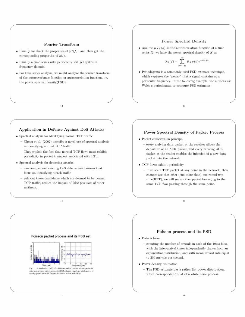
Poisson process and its PSD

• Data is from

– counting the number of arrivals in each of the 10ms bins,with the inter-arrival times independently drawn from anexponential distribution, and with mean arrival rate equalto 200 arrivals per second.

• Power density estimation

– The PSD estimate has a rather flat power distribution,which corresponds to that of a white noise process.

18

�

�

�

�19

�

�

�

�

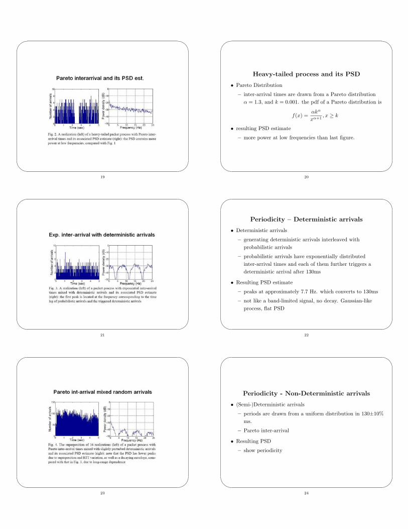
Heavy-tailed process and its PSD

• Pareto Distribution

– inter-arrival times are drawn from a Pareto distributionα = 1.3, and k = 0.001. the pdf of a Pareto distribution is

f(x) =αkα

xα+1, x ≥ k

• resulting PSD estimate

– more power at low frequencies than last figure.

20

�

�

�

�21

�

�

�

�

Periodicity – Deterministic arrivals

• Deterministic arrivals

– generating deterministic arrivals interleaved withprobabilistic arrivals

– probabilistic arrivals have exponentially distributedinter-arrival times and each of them further triggers adeterministic arrival after 130ms

• Resulting PSD estimate

– peaks at approximately 7.7 Hz. which converts to 130ms

– not like a band-limited signal, no decay. Gaussian-likeprocess, flat PSD

22

�

�

�

�23

�

�

�

�

Periodicity - Non-Deterministic arrivals

• (Semi-)Deterministic arrivals

– periods are drawn from a uniform distribution in 130±10%ms.

– Pareto inter-arrival

• Resulting PSD

– show periodicity

24

�

�

�

�

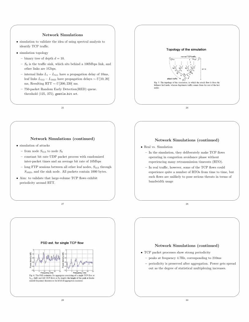
Network Simulations

• simulation to validate the idea of using spectral analysis toidentify TCP traffic.

• simulation topology

– binary tree of depth d = 10.

– S0 is the traffic sink, which sits behind a 100Mbps link, andother links are 1Gbps.

– internal links L1 − L511 have a propagation delay of 10ms,leaf links L512 − L1023 have propagation delays ∼ U [10, 20]ms, Resulting RTT ∼ U [200, 220] ms.

– 750-packet Random Early Detection(RED) queue.threshold (125, 375), gentle bit set.

25

�

�

�

�26

�

�

�

�

Network Simulations (continued)

• simulation of attacks

– from node S513 to node S0

– constant bit rate UDP packet process with randomizedinter-packet times and an average bit rate of 10Mbps

– long FTP sessions between all other leaf nodes, S513 throughS1023, and the sink node. All packets contain 1000 bytes.

• Aim: to validate that large-volume TCP flows exhibitperiodicity around RTT.

27

�

�

�

�

Network Simulations (continued)

• Real vs. Simulation

– In the simulation, they deliberately make TCP flowsoperating in congestion avoidance phase withoutexperiencing many retransmission timeouts (RTO).

– In real traffic, however, some of the TCP flows couldexperience quite a number of RTOs from time to time, butsuch flows are unlikely to pose serious threats in terms ofbandwidth usage

28

�

�

�

�29

�

�

�

�

Network Simulations (continued)

• TCP packet processes show strong periodicity

– peaks at frequency 4.7Hz, corresponding to 210ms

– periodicity is preserved after aggregation. Power gets spreadout as the degree of statistical multiplexing increases.

30

�

�

�

�31

�

�

�

�

Network Simulations (continued)

• The height of the first peak decreases as level of statisticalmultiplexing in an aggregate of TCP flows increases.

• Whether the aggregate has been contaminated by attack flows.

32

�

�

�

�

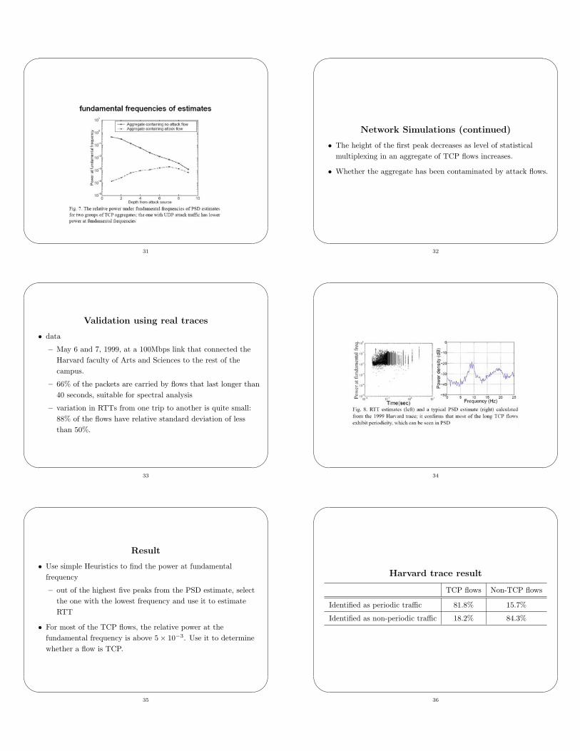
Validation using real traces

• data

– May 6 and 7, 1999, at a 100Mbps link that connected theHarvard faculty of Arts and Sciences to the rest of thecampus.

– 66% of the packets are carried by flows that last longer than40 seconds, suitable for spectral analysis

– variation in RTTs from one trip to another is quite small:88% of the flows have relative standard deviation of lessthan 50%.

33

�

�

�

�34

�

�

�

�

Result

• Use simple Heuristics to find the power at fundamentalfrequency

– out of the highest five peaks from the PSD estimate, selectthe one with the lowest frequency and use it to estimateRTT

• For most of the TCP flows, the relative power at thefundamental frequency is above 5 × 10−3. Use it to determinewhether a flow is TCP.

35

�

�

�

�

Harvard trace result

TCP flows Non-TCP flows

Identified as periodic traffic 81.8% 15.7%

Identified as non-periodic traffic 18.2% 84.3%

36

�

�

�

�

Discussion

• Not a independent anomalies detection method

– After we select candidate anomalies (connection, trace), thespectral analysis can help to say whether it is a normalTCP trace or not.

– do not provide when the attack exists. Need to examinemore.

• Attackers mimic the periodicity of normal TCP flows?

– Consider return paths along with forward paths, similarperiodicity

– Use closed-loop protocols to launching attacks? attackershave to consume an amount of resources comparable to thatof a normal TCP sender.

37

�

�

�

�

Discussion (continued)

• Best deal with long TCP flows, For short TCP flows the effectof their statistical multiplexing may outweigh their intrinsicperiodicity.

– Fortunately, short TCP flows usually represent a smallpercentage of the total TCP load to a network in terms ofpacket counts

38

�

�

�

�

Wavelet analysis

• Motivation

• Outline

– An example of wavelet analysis

– Definition of wavelet transform and its properties

– Wavelet methods for detection, results.

– Discussion

39

�

�

�

�

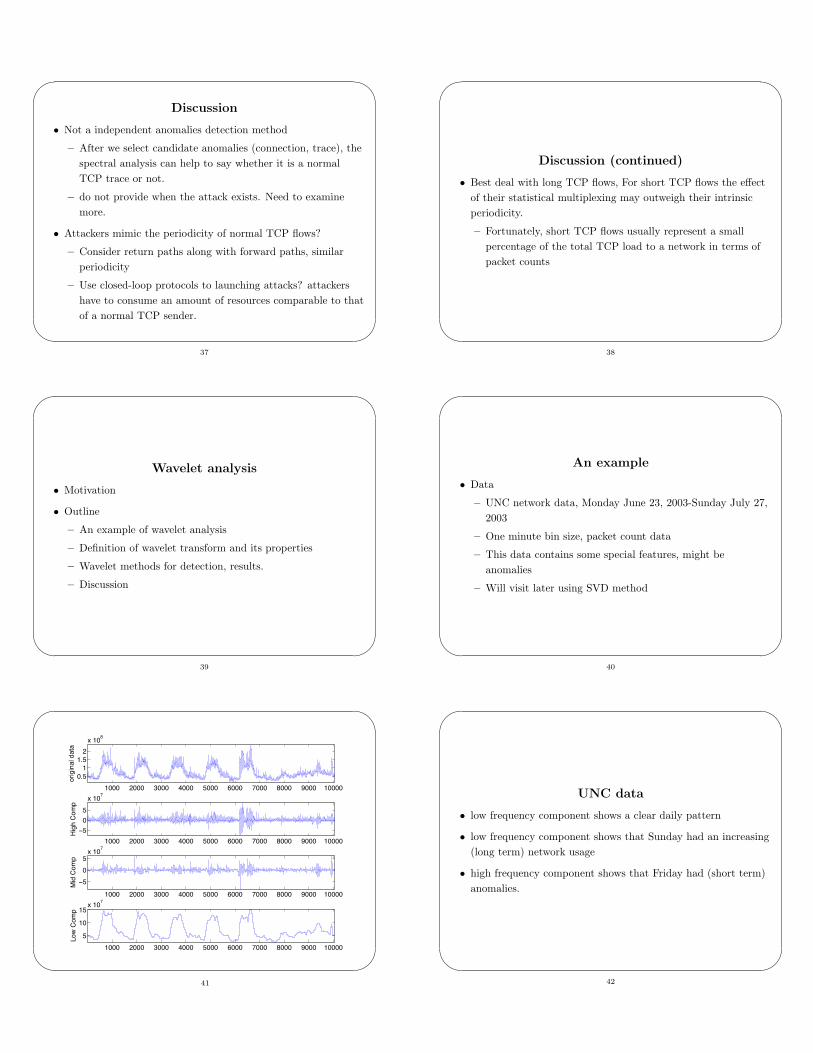
An example

• Data

– UNC network data, Monday June 23, 2003-Sunday July 27,2003

– One minute bin size, packet count data

– This data contains some special features, might beanomalies

– Will visit later using SVD method

40

�

�

�

�

1000 2000 3000 4000 5000 6000 7000 8000 9000 10000

0.51

1.52

x 108

orig

inal

dat

a

1000 2000 3000 4000 5000 6000 7000 8000 9000 10000

−5

0

5

x 107

Hig

h C

omp

1000 2000 3000 4000 5000 6000 7000 8000 9000 10000

−5

0

5x 10

7

Mid

Com

p

1000 2000 3000 4000 5000 6000 7000 8000 9000 10000

5

10

15x 10

7

Low

Com

p

41

�

�

�

�

UNC data

• low frequency component shows a clear daily pattern

• low frequency component shows that Sunday had an increasing(long term) network usage

• high frequency component shows that Friday had (short term)anomalies.

42

�

�

�

�

Good References

• Daubechies, I. “Ten Lectures on Wavelets”

• Mallat, S. “A Wavelet tour of Signal Processing”

• Percival, D.B. and Walden, A.T. “Wavelet Methods for TimeSeries Analysis”

The following introduction is mainly from Prof. Taqqu’s lecturenotes on “Long Range Dependence”, 2003, SAMSI.

43

�

�

�

�

Wavelet Transform

• Wavelet ψ(t)

A wavelet is a function ψ(t), t ∈ R, such that∫R

ψ(t)dt = 0

which satisfies some integrability conditions, for instanceψ ∈ L1(R) ∩ L2(R)

• N zero moments (also called vanishing moments)

– Wavelet ψ is said to have N zero moments if∫R

tkψ(t)dt = 0, k = 0, 1, · · · , N − 1 (3)

44

�

�

�

�

Typical examples of wavelets

• Derivatives of the standard normal density

ψ(t) =dn

dtn

(12π

e−t22

)

• Haar wavelets

ψ(t) =

⎧⎪⎪⎨⎪⎪⎩

1 0 ≤ t < 12

−1 12 ≤ t < 1

0 otherwise

• Daubechies wavelets

– multiresolution analysis, a family of wavelets which isindexed by their number of vanishing moments;orthonormal wavelet basis.

45

�

�

�

�

Dilation and translation of wavelets

• The functions

ψj,k(t) =1

2j/2ψ(2−jt − k) = 2−j/2ψ(2−j(t − 2jk)), j ∈ Z, k ∈ Z

are “dilations” and “translations” of ψ. The factors 2j and j

are called respectively the scale and the octave.

The normalization factor 2j/2 ensures that for all j ∈ Z andk ∈ Z ∫

R

ψ2j,k(t)dt =

∫R

ψ2(t)dt

46

�

�

�

�

Discrete wavelet transform

• Using the function {ψj,k, j, k ∈ Z} as set of filters, we can nowdefine the discrete wavelet transform DWT of a function (or ofthe sample path of a stochastic process) {X(t), t ∈ R} as

dj,k =∫

R

X(t)ψj,k(t)dt, j, k ∈ Z

The coefficients dj,k are called wavelet coefficients or details

47

�

�

�

�

Multiresolution analysis

• Multiresolution wavelets

– the wavelet ψ (“mother wavelet”) is defined through ascaling function, φ.

– both φ and ψ satisfy so-called two-scale equations

φ(t/2) =√

2Σnunφ(t − n)

ψ(t/2) =√

2Σnvnφ(t − n)

– the approximation coefficients aj,k is defined as

aj,k =∫

R

X(t)φj,k(t)dt, j ∈ Z, k ∈ Z

where φj,k(t) = 2−j/2φ(2−jt − k).

48

�

�

�

�49

�

�

�

�

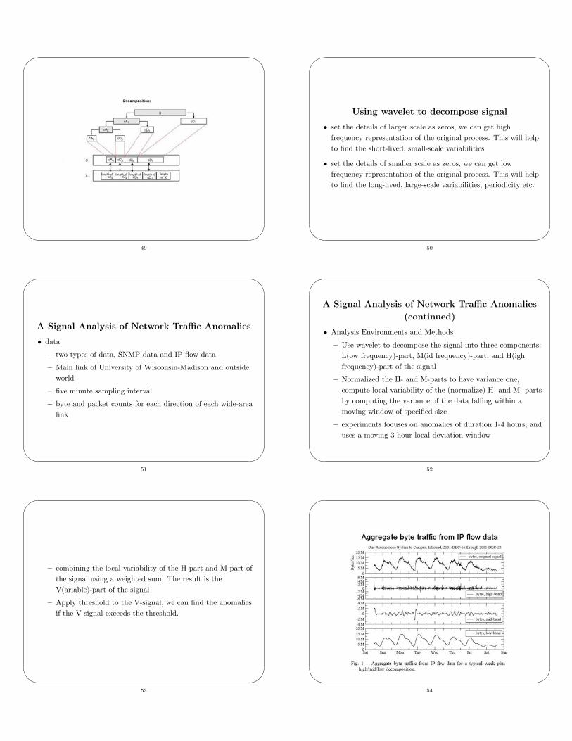
Using wavelet to decompose signal

• set the details of larger scale as zeros, we can get highfrequency representation of the original process. This will helpto find the short-lived, small-scale variabilities

• set the details of smaller scale as zeros, we can get lowfrequency representation of the original process. This will helpto find the long-lived, large-scale variabilities, periodicity etc.

50

�

�

�

�

A Signal Analysis of Network Traffic Anomalies

• data

– two types of data, SNMP data and IP flow data

– Main link of University of Wisconsin-Madison and outsideworld

– five minute sampling interval

– byte and packet counts for each direction of each wide-arealink

51

�

�

�

�

A Signal Analysis of Network Traffic Anomalies

(continued)

• Analysis Environments and Methods

– Use wavelet to decompose the signal into three components:L(ow frequency)-part, M(id frequency)-part, and H(ighfrequency)-part of the signal

– Normalized the H- and M-parts to have variance one,compute local variability of the (normalize) H- and M- partsby computing the variance of the data falling within amoving window of specified size

– experiments focuses on anomalies of duration 1-4 hours, anduses a moving 3-hour local deviation window

52

�

�

�

�

– combining the local variability of the H-part and M-part ofthe signal using a weighted sum. The result is theV(ariable)-part of the signal

– Apply threshold to the V-signal, we can find the anomaliesif the V-signal exceeds the threshold.

53

�

�

�

�54

�

�

�

�55

�

�

�

�

Characteristics of Ambient Traffic

• Byte counts of inbound traffic, IP flow data

– regular daily component of the signal is clear in the lowband

• Byte traffic for the same week, SNMP data

– nearly indistinguishable from the IP flow data

56

�

�

�

�57

�

�

�

�58

�

�

�

�

Characteristics of Flash Crowds

• flash crowds

– long-lived features which should be exposed by the mid- andlow-band filters

• outbound traffic (class-B network which contains an ftp mirrorserver)

– increasing at the low-band signal

• HTTP byte data

– more stable in the mid-band signal

59

�

�

�

�60

�

�

�

�61

�

�

�

�

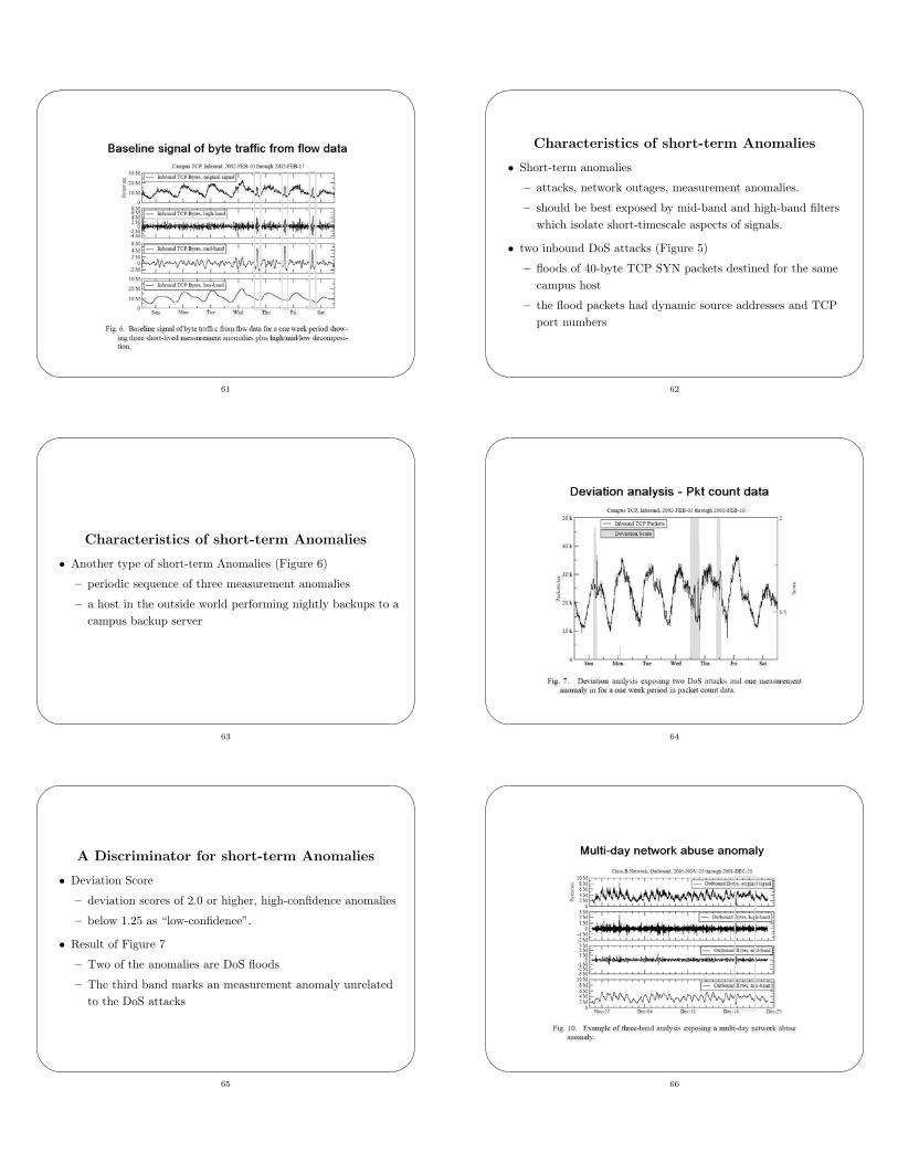
Characteristics of short-term Anomalies

• Short-term anomalies

– attacks, network outages, measurement anomalies.

– should be best exposed by mid-band and high-band filterswhich isolate short-timescale aspects of signals.

• two inbound DoS attacks (Figure 5)

– floods of 40-byte TCP SYN packets destined for the samecampus host

– the flood packets had dynamic source addresses and TCPport numbers

62

�

�

�

�

Characteristics of short-term Anomalies

• Another type of short-term Anomalies (Figure 6)

– periodic sequence of three measurement anomalies

– a host in the outside world performing nightly backups to acampus backup server

63

�

�

�

�64

�

�

�

�

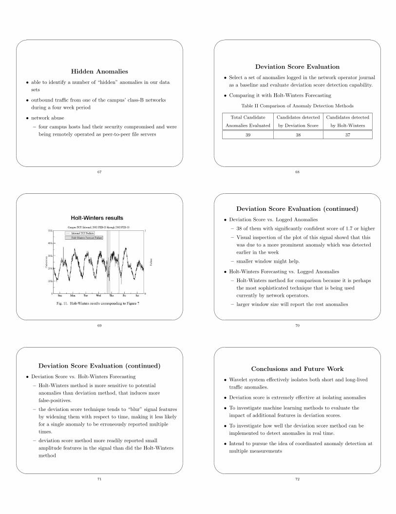
A Discriminator for short-term Anomalies

• Deviation Score

– deviation scores of 2.0 or higher, high-confidence anomalies

– below 1.25 as “low-confidence”.

• Result of Figure 7

– Two of the anomalies are DoS floods

– The third band marks an measurement anomaly unrelatedto the DoS attacks

65

�

�

�

�66

�

�

�

�

Hidden Anomalies

• able to identify a number of “hidden” anomalies in our datasets

• outbound traffic from one of the campus’ class-B networksduring a four week period

• network abuse

– four campus hosts had their security compromised and werebeing remotely operated as peer-to-peer file servers

67

�

�

�

�

Deviation Score Evaluation

• Select a set of anomalies logged in the network operator journalas a baseline and evaluate deviation score detection capability.

• Comparing it with Holt-Winters Forecasting

Table II Comparison of Anomaly Detection Methods

Total Candidate Candidates detected Candidates detected

Anomalies Evaluated by Deviation Score by Holt-Winters

39 38 37

68

�

�

�

�69

�

�

�

�

Deviation Score Evaluation (continued)

• Deviation Score vs. Logged Anomalies

– 38 of them with significantly confident score of 1.7 or higher

– Visual inspection of the plot of this signal showd that thiswas due to a more prominent anomaly which was detectedearlier in the week

– smaller window might help.

• Holt-Winters Forecasting vs. Logged Anomalies

– Holt-Winters method for comparison because it is perhapsthe most sophisticated technique that is being usedcurrently by network operators.

– larger window size will report the rest anomalies

70

�

�

�

�

Deviation Score Evaluation (continued)

• Deviation Score vs. Holt-Winters Forecasting

– Holt-Winters method is more sensitive to potentialanomalies than deviation method, that induces morefalse-positives.

– the deviation score technique tends to “blur” signal featuresby widening them with respect to time, making it less likelyfor a single anomaly to be erroneously reported multipletimes.

– deviation score method more readily reported smallamplitude features in the signal than did the Holt-Wintersmethod

71

�

�

�

�

Conclusions and Future Work

• Wavelet system effectively isolates both short and long-livedtraffic anomalies.

• Deviation score is extremely effective at isolating anomalies

• To investigate machine learning methods to evaluate theimpact of additional features in deviation scores.

• To investigate how well the deviation score method can beimplemented to detect anomalies in real time.

• Intend to pursue the idea of coordinated anomaly detection atmultiple measurements

72

�

�

�

�

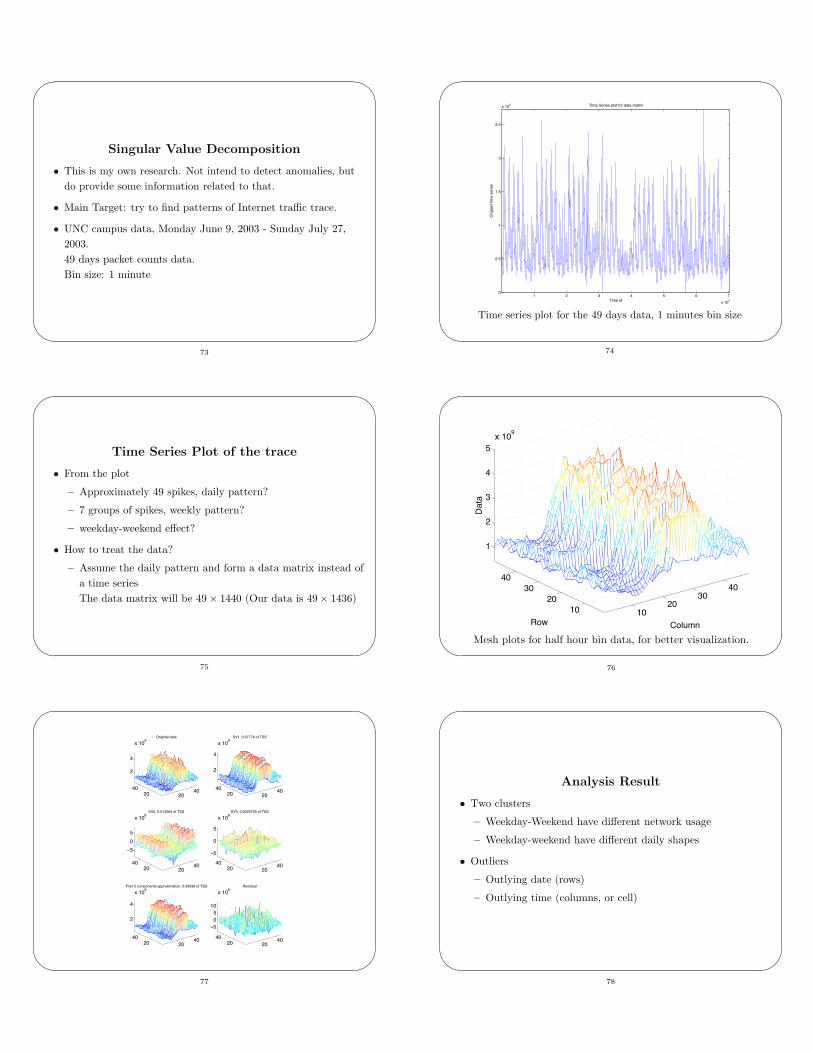
Singular Value Decomposition

• This is my own research. Not intend to detect anomalies, butdo provide some information related to that.

• Main Target: try to find patterns of Internet traffic trace.

• UNC campus data, Monday June 9, 2003 - Sunday July 27,2003.49 days packet counts data.Bin size: 1 minute

73

�

�

�

�1 2 3 4 5 6 7

x 104

0

0.5

1

1.5

2

2.5

x 108

Time id

Orig

ianl

tim

e se

ries

Time Series plot for data matrix

Time series plot for the 49 days data, 1 minutes bin size

74

�

�

�

�

Time Series Plot of the trace

• From the plot

– Approximately 49 spikes, daily pattern?

– 7 groups of spikes, weekly pattern?

– weekday-weekend effect?

• How to treat the data?

– Assume the daily pattern and form a data matrix instead ofa time seriesThe data matrix will be 49 × 1440 (Our data is 49 × 1436)

75

�

�

�

�10

2030

40

1020

3040

1

2

3

4

5x 10

9

ColumnRow

Dat

a

Mesh plots for half hour bin data, for better visualization.

76

�

�

�

�

204020

40

2

4

x 109

Original data

204020

40

2

4

x 109

SV1, 0.97774 of TSS

204020

40

−5

0

5

x 108

SV2, 0.013064 of TSS

204020

40

−5

0

5

x 108

SV3, 0.0025745 of TSS

204020

40

2

4

x 109

First 3 components approximation, 0.99338 of TSS

204020

40

−505

10

x 108

Residual

77

�

�

�

�

Analysis Result

• Two clusters

– Weekday-Weekend have different network usage

– Weekday-weekend have different daily shapes

• Outliers

– Outlying date (rows)

– Outlying time (columns, or cell)

78

�

�

�

�

Definition of Singular Value Decomposition

Singular Value Decomposition of a data matrix X = (Xij)m×n withrank(X) = r is defined as

X = USV T (4)

= s1u1vT1 + · · · + srurvT

r (5)

where U = (u1,u2, · · · ,ur), V = (v1,v2, · · · ,vr),S = diag{s1, s2, · · · , sr} with s1 ≥ s2 ≥ · · · ≥ sr. {ui} and {vi} arecalled singular columns and singular rows respectively; {si} arecalled singular values; and matrices {siuivT

i }(i = 1, · · · , r) arereferred to as SVD components.

79

�

�

�

�

Properties of Singular Columns and Rows

• Singular Columns (u’s)

– ui forms orthonormal basis for columns spaces spanned bythe columns of the data matrix X.

– ui also gives relative scores of original data X projects onthe corresponding vi.

• Singular Rows (v’s)

– vi forms orthonormal basis for rows spaces spanned by therows of the data matrix X.

– vi also gives relative scores of original data X projects onthe corresponding ui.

80

�

�

�

�

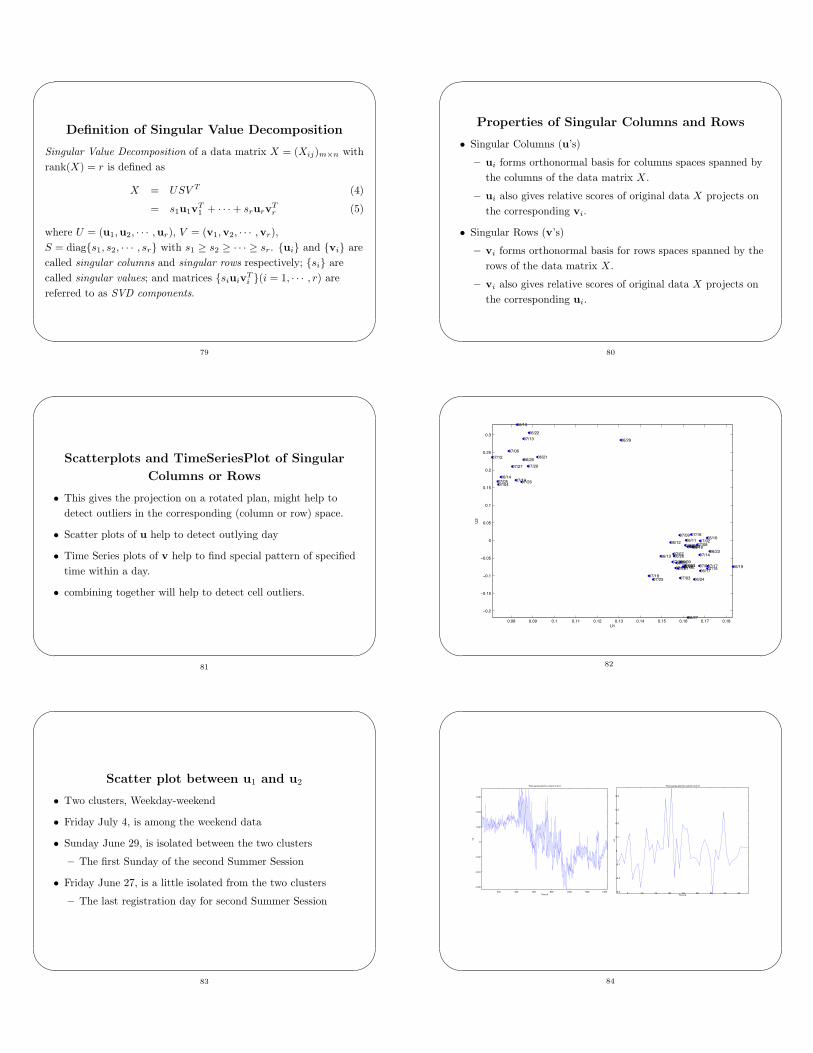
Scatterplots and TimeSeriesPlot of Singular

Columns or Rows

• This gives the projection on a rotated plan, might help todetect outliers in the corresponding (column or row) space.

• Scatter plots of u help to detect outlying day

• Time Series plots of v help to find special pattern of specifiedtime within a day.

• combining together will help to detect cell outliers.

81

�

�

�

�0.08 0.09 0.1 0.11 0.12 0.13 0.14 0.15 0.16 0.17 0.18

−0.2

−0.15

−0.1

−0.05

0

0.05

0.1

0.15

0.2

0.25

0.3

U1

U2

06/09

06/10

06/1106/12

06/13

06/14

06/15

06/16

06/17

06/18

06/1906/20

06/21

06/22

06/23

06/24

06/25

06/26

06/27

06/28

06/29

06/30

07/01

07/02

07/03

07/0407/05

07/06

07/07

07/08

07/09

07/10

07/11

07/12

07/13

07/14

07/15

07/16

07/17

07/18

07/19

07/20

07/2107/2207/2307/24

07/25

07/26

07/27

82

�

�

�

�

Scatter plot between u1 and u2

• Two clusters, Weekday-weekend

• Friday July 4, is among the weekend data

• Sunday June 29, is isolated between the two clusters

– The first Sunday of the second Summer Session

• Friday June 27, is a little isolated from the two clusters

– The last registration day for second Summer Session

83

�

�

�

�

200 400 600 800 1000 1200 1400

−0.06

−0.04

−0.02

0

0.02

0.04

0.06

Time id

v3

Time series plot for column 3 of V

5 10 15 20 25 30 35 40 45−0.3

−0.2

−0.1

0

0.1

0.2

0.3

0.4

Time id

u3

Time series plot for column 3 of U

84

�

�

�

�

Time Series of u3 and v3

• v3

– 420-600 of v3 is with higher variability.

• u3

– Row 19, 21 is with large projection. Which indicates thatRow 19 and Row 21 contribute a lot on v3.

• Last registration day

85

�

�

�

�

Multiple Time Series and Multivariate Methods

• Anomaly detection base on modeling and analysis of traffic onall links simultaneously. Jeff presented several papers already.This might induced Multiple Time Series Methods.

• Anomaly might not be detected from a single measurement,but possibly be detected from analysis of several measurementstogether.

• The correlation between time series, or measurements mightmask some anomalies (outlier).

86

�

�

�

�

Measurements

• Measurements at single link

– packet counts, bytes, etc.

– simple statistics of network information, entropy of packet,etc.

• Measurement of whole network(?)

– flow packet, bytes etc.

87

�

�

�

�

Multivariate Outlier Detection

• Outlier in multivariate sense is much harder to detect.

• Univariate outlier detection method is not enough.

• Outlier might be masked for the multivariate correlation.

• Resent research topic in Statistics

88

�

�

�

�

An example

• To show one multivariate outlier detection method

• To illustrate the outlier might not be detected from singlemeasurement outlier detection method

• Problem of the example: do not know the false positive andfalse negative rate

89

�

�

�

�

Idea of the detection

• The multivariate data forms point cloud in high-dimensionalspace. The point cloud might consist of one main cluster, andother points or small clusters out of it.

• Calculate the distance of each point to the center point of themain cluster, and define those with large value as(multivariate) outliers.

90

�

�

�

�

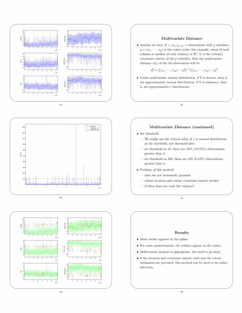
1 2 3 4 5 6 7

x 104

0

2

4

6

8

10

12

pack

et

1 2 3 4 5 6 7

x 104

−2

0

2

4

6

8

byte

1 2 3 4 5 6 7

x 104

−4

−2

0

2

4

6

8

flow

1 2 3 4 5 6 7

x 104

−3

−2

−1

0

1

2

3

H(p

kt s

ize)

1 2 3 4 5 6 7

x 104

−10

−5

0

H(s

rc p

ort)

1 2 3 4 5 6 7

x 104

−6

−4

−2

0

2

H(d

st p

ort)

91

�

�

�

�

Multivariate Distance

• Assume we have X = (xij)n×p, n observations with p variables.µ = (u1, · · · , up) is the center point (fox example, mean of eachcolumn or median of each column) in R

p, Σ is the (robust)covariance matrix of the p variables, then the multivariatedistance (di) of the ith observation will be

d2i = [(xi1, · · · , xip) − µ]Σ−1[(xi1, · · · , xip) − µ]T

• Under multivariate normal distribution, if Σ is known, then di

are approximately normal distribution. if Σ is unknown, thendi are approximately t distribution.

92

�

�

�

�1 2 3 4 5 6 7

x 104

100

200

300

400

500

600

700

800

900

1000

dist

ance

distancethreshold=10threshold=100

93

�

�

�

�

Multivariate Distance (continued)

• Set threshold

– We might use the critical value of t or normal distributionas the threshold, not discussed here.

– set threshold as 10, there are 7871 (10.75%) observationsgreater than it.

– set threshold as 100, there are 105 (0.14%) observationsgreater than it.

• Problem of this method

– data are not necessarily gaussian

– robust location and robust covariance matrix needed

– if there does not exist the variance?

94

�

�

�

�

1 2 3 4 5 6 7

x 104

0

2

4

6

8

10

12

pack

et

1 2 3 4 5 6 7

x 104

−2

0

2

4

6

8

byte

1 2 3 4 5 6 7

x 104

−4

−2

0

2

4

6

8

flow

1 2 3 4 5 6 7

x 104

−3

−2

−1

0

1

2

3

H(p

kt s

ize)

1 2 3 4 5 6 7

x 104

−10

−5

0

H(s

rc p

ort)

1 2 3 4 5 6 7

x 104

−6

−4

−2

0

2

H(d

st p

ort)

95

�

�

�

�

Results

• Most outlier appears in the spikes

• For some measurements, the outliers appear in the center.

• Multivariate analysis is appropriate, but need to go deep.

• if the location and covariance matrix exist and the robustestimation are provided, this method can be used to do onlinedetection.

96

�

�

�

�

PCA(SVD) Method

• Another popular method to detect multivariate outliers

• Basically project the observations onto the principal direction,and find extreme values with respect to those projections.

• Statisticians also form some statistics of the former projectionsto detect outliers

• Flow data already talked by Jeff.

97

�

�

�

�

Part III – Further Work

98

�

�

�

�

Statistical Properties of Normal traffic and

Anomalies

• Which measurements best fit for analysis

• Correlation between measurements

• Signals of existing anomalies

99

�

�

�

�

New Statistical Methods

• Anomalies might affect the normal traffic decomposition.robust method might help, decrease false negative.

• Statistical Theory under non-Gaussian, Long range dependenceor heavy tailed sample

100

�

�

�

�

Multi-Scale Detection

• Anomalies vary from different scales. One scale statisticalmethod is not appropriate?

• Multivariate Wavelet Method?

• Multi-Scale data?

101

�

�

�

�

Online Detection

• Current work mostly done at offline sense

• Online detection is essential

• Update algorithm every fix time interval

• Processing time should be short, response time should be quick,false negative and false positive should be as small as possible

102

�

�

�

�

References

[1] P. Barford, J. Kline, D. Plonka and A. Ron, (2002) A SignalAnalysis of Network Traffic Anomalies, Proceedings of the 2ndACM SIGCOMM Workshop on Internet Measurment,Marseille, France, pp 71-82.

[2] Chen-Mou Cheng, H. T. Kung and Koan-Sin Tan, (2002) Use ofSpectral Analysis in Defense Against DoS Attacks Proceedingsof IEEE GLOBECOM 2002, Taipei, Taiwan.

[3] Laura Feinstein, Dan Schnackenberg, Ravindra Balupari andDarrell Kindred, (2003) Statistical Approaches to DDoS AttackDetection and Response, Proceedings of the DARPAInformation Survivability Conference and Exposition(DISCEX03), Washington, DC.

103