Transaction Processing John Ortiz. Lecture 19Transaction Processing2 Introduction Transactions are motivated by two of the properties of DBMS's discussed

Transaction Processing

John Ortiz

Lecture 19 Transaction Processing 2

Introduction Transactions are motivated by two of the

properties of DBMS's discussed way back in our first lecture: Multi-user database access Safe from system crashes

Main issues: How to model concurrent execution of

user programs? How to guarantee acceptable DB

behavior? How to deal with system crashes?


Why Concurrency? Allowing only serial execution of user

programs may cause poor system performance Low throughput, long response time Poor resource utilization (CPU, disks)

Concurrent execution of user programs is essential for good DBMS performance. Because disk accesses are frequent, and

relatively slow, it is important to keep the CPU humming by working on several user programs concurrently


Example: Why Concurrency? Assume each users’ program uses CPU and

I/O resources (disks) in an interleaved fashion:

CPU, R(X), CPU, W(X) Suppose each CPU request takes 1 time unit

and each I/O request takes 5 time units. For a 2 GHz Machine, one clock tick is ½ ns

An 8 millisecond seek time is 8000 microseconds, which is 8,000,000 ns

Clearly the CPU can get quite a bit done while the disk is searching for a block


Example: Why Concurrency?

T1T2T3T4 Time

CPUI/O

Serial scheduleTime units = 48

T1

T2T3T4 Time

CPUI/O

Non-serial scheduleTime units = 41


Example: Why Concurrency?

T1T2T3T4 Time

CPUI/O

Serial scheduleTime units = 48

T1

T2

T3

T4 Time

CPUI/O 1I/O 2

Non-serial scheduleTime units = 22Use 2 disks


Transaction A user program may carry out many

operations on data retrieved from database, but DBMS is only concerned about what data is read/written from/to the database (on disk)

A transaction is a sequence of database actions that is considered as a unit of work DB actions: read (R(X)), write (W(X)),

commit, abort Represent DBMS’s abstract view of

Interact user sessions Execution of user programs


Example: Transaction Account(Ano, Name, Type, Balance) A user want to

update Account set Balance = Balance – 50 where Ano = 10001

update Account set Balance = Balance + 50 where Ano = 12300

Let A be account w/ Ano=10001, B be account w/ Ano=12300. The transaction is

R(A), W(A), R(B), W(B)


States of a Transaction

active

commit partiallycommitted

failed

committed

abortedabort

failure

exception

end transaction

begintransaction

read/write


Consistency of Transaction Each transaction must leave the database

in a consistent state if the DB is consistent when the transaction begins. DBMS will enforce some ICs, depending

on the ICs declared in CREATE TABLE statements.

Beyond this, the DBMS does not really understand the semantics of the data. (e.g., it does not understand how the interest on a bank account is computed).


Atomicity of Transactions A transaction might commit after

completing all its actions, or it could abort (or be aborted by the DBMS) after executing some actions.

A very important property guaranteed by the DBMS for all transactions is that they are atomic. That is, a user can think of a transaction as always executing all its actions in one step, or not executing any actions at all. DBMS logs all actions so that it can undo

the actions of aborted transactions.


Example: Why Atomicity? Account(Ano, Name, Type, Balance) A user want to

update Account set Balance = Balance – 50 where Ano = 10001

update Account set Balance = Balance + 50 where Ano = 12300

System crashed in the middle Possible outcome w/o recovery:

$50 transferred or lost The operations must be done as a unit


Durability DBMS often save data in main memory

buffer to improve system efficiency. Data in buffer is volatile (may get lost if system crashes)

When a transaction commits, DBMS must guarantee that all updates make by the transaction will not be lost even if the system crashes later DBMS uses the log to redo actions of

committed transactions if necessary


Isolation Users submit transactions, and can think of

each transaction as executing by itself (in isolation) Concurrency is achieved by the DBMS,

which interleaves actions (reads/writes of DB objects) of various transactions

DBMS guarantees that interleaving transactions do not interfere with each other


Example: Why Isolation? Two users (programs) do this at the same

time User 1: update Student set GPA = 3.7

where SID = 123 User 2: update Student set Major = ‘CS’

where SID = 123 Sequence of events: for each user, read

tuple, modify attribute, write tuple. Possible outcomes w/o concurrency control:

one change or both


Example: Why Isolation? Emp(EID, Name, Dept, Sal, Start, Loc) User 1: update Emp set Dept = ‘Sales’

where Loc = ‘Downtown' User 2: update Emp set Start = 3/1/00

where Start = 2/29/00 Possible outcomes w/o concurrency control:

each tuple has one change or both, may be inconsistent across tuples


Example: Interleaved Transactions Consider two transactions:

T1: BEGIN A=A+100, B=B-100 ENDT2: BEGIN A=1.06*A, B=1.06*B END

T1: A=A+100, B=B-100 T2: A=1.06*A, B=1.06*B

T1: A=A+100, B=B-100 T2: A=1.06*A, B=1.06*B

One possible interleaved execution:

It is OK. But what about another interleaving?


Schedule: Modeling Concurrency Schedule: a sequence of operations from a

set of transactions, where operations from any one transaction are in their original order

Notation:T1 T2 R(A) W(A) R(B) W(B) R(C) W(C)

R1(A), W1(A), R2(B), W2(B), R1(C), W1(C)

Ri(X): read X by Ti

Wi(X): write X by Ti


Schedule (cont.) Represents some actual sequence of

database actions. In a complete schedule, each transaction

ends in commit or abort. A schedule transforms database from an

initial state to a final state

Initialstate

Finalstate

A schedule


Schedule (cont.) Assume a consistent initial state A representation of an execution of

operations from a set of transactions Ignore

aborted transactions Incomplete (not yet committed) transactions

Operations in a schedule conflict if1. They belong to different transactions2. They access the same data item3. At least one item is a write operation


Anomalies with Concurrency Interleaving transactions may cause many

kinds of consistency problems Reading Uncommitted Data ( “dirty reads”):

Unrepeatable Reads:

Overwriting Uncommitted Data (lost update):

R1(A), W1(A), R2(A), W2(A), C2, R1(B), A1

R1(A), R2(A), W2(A), C2, R1(A), W1(A), C1

R1(A), R2(A), W2(A), W1(A)


Anomalies with Concurrency Incorrect Summary Problem

Data items may be changed by one transaction while another transaction is in the process of calculating an aggregate value

A correct “sum” may be obtained prior to any change, or immediately after any change


Serial Schedule An acceptable schedule must transform

database from a consistent state to another consistent state

Serial schedule : one transaction runs entirely before the next transaction starts.

T1: R(X), W(X)T2: R(X), W(X)

R1(X) W1(X) C1 R2(X) W2(X) C2

R2(X) W2(X) C2 R1(X) W1(X) C1

Serial

R1(X) R2(X) W2(X) W1(X) C1 C2 Non-serial


Serial Schedule IS Acceptable Serial schedules guarantee transaction

isolation & consistency Different serial schedules can have different

final states N transactions may form N! different

serial schedules Any state from a serial schedule is

acceptable – DBMS makes no guarantee about the order in which transactions are executed


Example: Serial Schedules T1: R(X), X=X+10, W(X) T2: R(X), X=X*2, W(X)

InitialX = 20

R2(X) W2(X) C2 R1(X) W1(X) C1S2:

FinalX = 50

R1(X) W1(X) C1 R2(X) W2(X) C2S1:

FinalX = 60


Is Non-Serial Schedule Acceptable?

T1: R(X), X=X*2, W(X), R(Y), Y=Y-5, W(Y)T2: R(X), X=X+10, W(X)

InitialX=20Y=35

R1(X) W1(X) R2(X) W2(X) R1(Y) W1(Y) C1 C2 S1:

finalX=50Y=30

R1(X) W1(X) R1(Y) W1(Y) C1 R2(X) W2(X) C2 S2:


Serializable Schedules Serializable schedule: Equivalent to a serial

schedule of committed transactions. Non-serial (allow concurrent execution) Acceptable (final state is what some

serial schedule would have produced) Types of Serializable schedules: depend on

how the equivalency is defined Conflict: based on conflict operations View: based on viewing of data

Ex: p.645, text does not show commits


Lock-Based Concurrency Control Strict Two-phase Locking (Strict 2PL)

Protocol: Each transaction must obtain a S (shared)

lock on object before reading, and an X (exclusive) lock on object before writing.

All locks held by a transaction are released when the transaction completes

If a transaction holds an X lock on an object, no other transaction can get a lock (S or X) on that object.

Strict 2PL allows only serializable schedules.


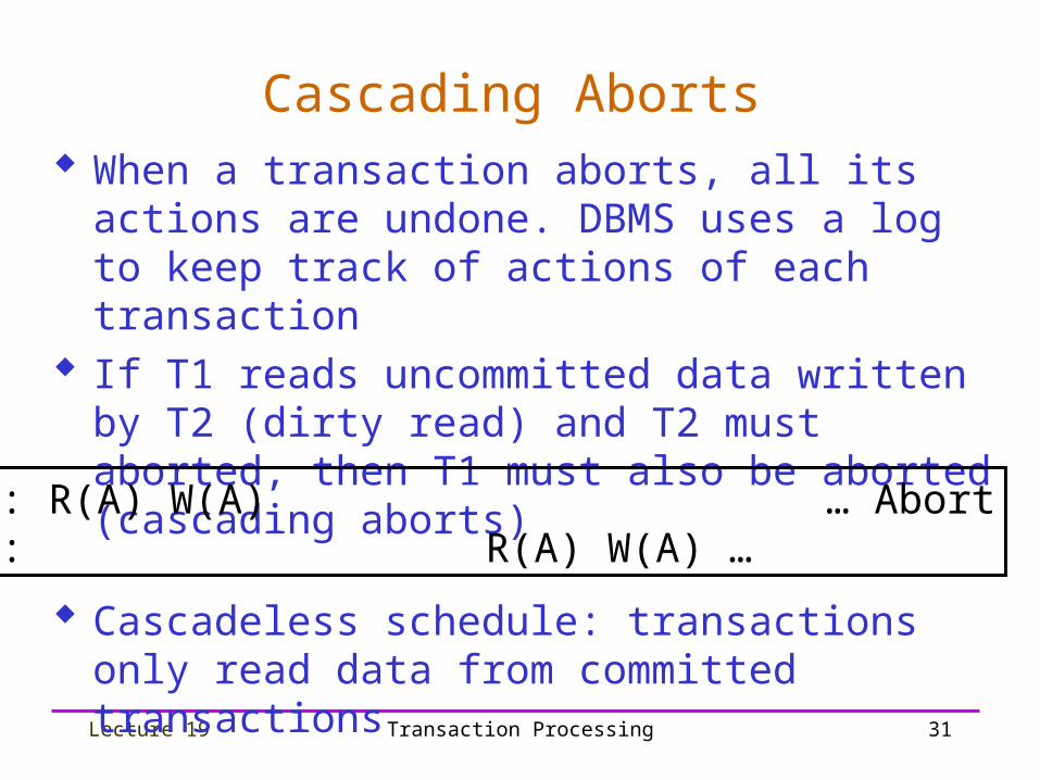
Cascading Aborts When a transaction aborts, all its actions

are undone. DBMS uses a log to keep track of actions of each transaction

If T1 reads uncommitted data written by T2 (dirty read) and T2 must aborted, then T1 must also be aborted (cascading aborts)

Cascadeless schedule: transactions only read data from committed transactions

T1: R(A) W(A) … AbortT2: R(A) W(A) …


Recoverability If a transaction fails, the DBMS must return

the DB to its previous state1. Computer failure – hw, sw, network, memory

error2. Transaction error – erroneous input, divison by

zero3. Local errors – insufficient funds, data not found4. Concurrency control enforcement – transaction

aborted5. Disk failure – hard disk crash (listed in text but

not much different from 1.)6. Physical catastrophe – power, theft, fire, etc.


Recoverability If T1 reads data from T2, commits and then

T2 needs to abort, what should DBMS do? This situation is undesirable! A schedule is recoverable if very transaction

commits only after all transactions from which it reads data commit.

Cascadeless schedules are recoverable (but not vice-versa!).

Real systems typically ensure that only recoverable schedules arise (through locking).


Summary Transactions model DBMS’ view of user

programs Concurrency control and recovery are

important issues in DBMSs Transactions must have ACID properties

Atomicity Consistency Isolation Durability

C & I are guaranteed by concurrency control

A & D are guaranteed by crash recovery


Summary (cont.) Schedule models concurrent execution of

transactions Conflicts arise when two transactions

access the same object, and one of the transactions is modifying it

Serial execution is our model of correctness Serializability allows us to “simulate” serial

execution with better performance Concurrent execution should avoid cascade

abort and be recoverable

Documents

Transaction Processing John Ortiz. Lecture 19Transaction Processing2 Introduction Transactions are motivated by two of the properties of DBMS's discussed