Embed Size (px)
Citation preview
SIGNAL ANALYSIS USING AUTOREGRESSIVE MODELS
OF AMPLITUDE MODULATION
by
Sriram Ganapathy
A dissertation submitted to The Johns Hopkins University in conformity with the
requirements for the degree of Doctor of Philosophy.
Baltimore, Maryland
January, 2012
c© Sriram Ganapathy 2012
All rights reserved
Abstract
Conventional speech analysis techniques are based on estimating the spectral
content of relatively short (about 10-20 ms) segments of the signal. However, an
alternate way to describe a speech signal is a summation of amplitude modulated
frequency bands, where each frequency band consists of a smooth envelope (gross
structure) modulating a carrier signal (fine structure). The analytic signal (AS) forms
a suitable candidate for such an envelope-carrier decomposition with the squared
magnitude of the AS, called the Hilbert envelope, representing the smooth structure
and the phase component of the AS representing the fine structure. However, the
computation of analytic signal is cumbersome and theoretically requires the use of a
filter with infinite impulse response.
In this thesis, we adopt an auto-regressive (AR) modeling approach for esti-
mating the Hilbert envelope of the signal. The Hilbert envelope represents the evo-
lution of signal energy in time domain. This model, referred to as frequency domain
linear prediction (FDLP), is based on the application of linear prediction on discrete
cosine transform of the signal. Thus, FDLP is dual process to the conventional time
ii

ABSTRACT
domain linear prediction (TDLP).
Just like conventional AR models, the FDLP model describes the perceptu-
ally dominant peaks and removes the finer-scale detail. This suppression of detail is
particularly useful for parametric representation of speech/audio signals, where the
goal is to summarize the general form of the signal. We show several applications
of the FDLP model for speech and audio processing systems. As a unified model
of speech and audio signals, we apply the FDLP technique for wide-band high fi-
delity audio coding. In subjective evaluations, the FDLP codec compares well with
state-of-art speech/audio codecs.
In order to derive robust representation in the presence of reverberation and
channel distortions, we propose a gain normalization procedure for FDLP envelopes.
The gain normalization suppresses the effect of long-term convolutive distortions in
sub-bands of speech. We apply the gain-normalized FDLP envelopes for feature
extraction in speaker, speech and phoneme recognition experiments. In these exper-
iments, the FDLP features provide significant improvements over the conventional
techniques in noisy and reverberant environments.
Thesis Committee
Dan Ellis, Thomas Quatieri, Trac D Tran, Mounya Elhilali, Hynek Hermansky
iii
Acknowledgments
I am immensely grateful to Prof. Hynek Hermansky for providing me with
freedom and perseverance throughput my graduate life. During this period, he had
allowed me to follow my passion and interests without enforcing his requirements.
This resulted in a great deal of enjoyment in my dissertation research.
I am infinitely indebted to Samuel Thomas for the collaborative work. Many
of the contributions in this thesis would not have been possible without his involve-
ment and ideas. I express my gratitude to Sivaram Garimella for his involvement in
my research as well as his patience in correcting the thesis. Other members of my
JHU lab who were involved with my work are Harish Mallidi, Padmanabhan Rajan,
Aren Jansen, Thomas Janu and Vijay Peddinti. I would also like to acknowledge var-
ious other project members including Xinhui Zhou, Daniel Romero, David Gelbart,
Guenter Hirsch, Marios Athineos, Jason Pelecanos and Harinath Garudadri.
Since my graduate research was partly done at Idiap research institute in
Switzerland, I would like to thank my Idiap colleagues for their support and help
during the initial part of my thesis. These colleagues include Petr Motlicek, Joel
iv
ACKNOWLEDGMENTS
Pinto, Fabio Valente, Deepu Vijayasenan, Tamara Tosic and Mathew Doss. The
audio coding work presented in this thesis was based on the team-work with Petr
Motlicek.
On a personal level, I express my gratitude for the love, support and encour-
agement from my family members Geetha, Ganapathy, Gomathy and Priya and my
friends Rajalekshmi, Pradeepa, Basavaraj and Sudha.
Last but not least, I am grateful to the suggestions from my thesis commit-
tee members - Mounya Elhilali, Trac Tran, Dan Ellis and Thomas Quatieri. Their
comments and ideas resulted in improving the thesis work significantly.
v
Contents
Abstract ii
Acknowledgments iv
List of Tables xii
List of Figures xiii
1 Introduction 1
1.1 Motivation . . . . . . . . . . . . . . . . . . . . . . . . . . . . . . . . . . . . 1
1.1.1 Conventional Signal Analysis . . . . . . . . . . . . . . . . . . . . . . 1
1.1.2 Conventional Analysis Versus Proposed Approach . . . . . . . . . . 2
1.2 Past Modulation Approaches . . . . . . . . . . . . . . . . . . . . . . . . . . 6
1.2.1 Demodulation Methodologies . . . . . . . . . . . . . . . . . . . . . . 7
1.2.2 Applications of Past Approaches . . . . . . . . . . . . . . . . . . . . 10
1.2.3 Comments on Past Methodologies . . . . . . . . . . . . . . . . . . . 13
1.3 Outline of Contributions . . . . . . . . . . . . . . . . . . . . . . . . . . . . . 14
1.4 Road Map for Rest of the Thesis . . . . . . . . . . . . . . . . . . . . . . . . 15
vi
CONTENTS
2 Frequency Domain Linear Prediction (FDLP) 19
2.1 Chapter Outline . . . . . . . . . . . . . . . . . . . . . . . . . . . . . . . . . 19
2.2 Properties of Analytic signal . . . . . . . . . . . . . . . . . . . . . . . . . . . 20
2.3 Past Approaches in AR modeling of Hilbert Envelopes . . . . . . . . . . . . 22
2.3.1 Temporal Noise Shaping (TNS) . . . . . . . . . . . . . . . . . . . . . 22
2.3.2 Linear Prediction in Spectral Domain (LPSD) . . . . . . . . . . . . 23
2.3.3 AR Modeling of Temporal Envelopes . . . . . . . . . . . . . . . . . . 24
2.4 Linear Prediction . . . . . . . . . . . . . . . . . . . . . . . . . . . . . . . . . 25
2.4.1 Time Domain Linear Prediction (TDLP) . . . . . . . . . . . . . . . 25
2.5 Frequency Domain Linear Prediction (FDLP) . . . . . . . . . . . . . . . . . 29
2.5.1 Discrete-Time Analytic Signal . . . . . . . . . . . . . . . . . . . . . . 30
2.5.2 Relation between Auto-correlations of DCT and Hilbert Envelope . 31
2.5.3 Examples . . . . . . . . . . . . . . . . . . . . . . . . . . . . . . . . . 34
2.6 Temporal Resolution Analysis in FDLP . . . . . . . . . . . . . . . . . . . . 38
2.6.1 Defining the Temporal Resolution . . . . . . . . . . . . . . . . . . . 39
2.6.2 Effect of Various Factors on Resolution . . . . . . . . . . . . . . . . 40
2.7 Chapter Summary . . . . . . . . . . . . . . . . . . . . . . . . . . . . . . . . 42
3 Gain Normalization of FDLP Envelopes 44
3.1 Chapter Outline . . . . . . . . . . . . . . . . . . . . . . . . . . . . . . . . . 44
3.2 Room Reverberation . . . . . . . . . . . . . . . . . . . . . . . . . . . . . . . 45
3.3 Past Approaches For Suppressing Convolutive Artifacts . . . . . . . . . . . 47
3.3.1 Cepstral Mean Subtraction (CMS) . . . . . . . . . . . . . . . . . . . 47
vii
CONTENTS
3.3.2 Log-DFT Mean Normalization (LDMN) . . . . . . . . . . . . . . . . 48
3.3.3 Long-term Log Spectral Subtraction (LTLSS) . . . . . . . . . . . . . 48
3.4 Envelope Convolution Model . . . . . . . . . . . . . . . . . . . . . . . . . . 49
3.5 Robust Envelope Estimation With Gain Normalization . . . . . . . . . . . . 51
3.6 Suppressing Reverberation With Gain Normalization . . . . . . . . . . . . . 56
3.7 Chapter Summary . . . . . . . . . . . . . . . . . . . . . . . . . . . . . . . . 58
4 Short-Term Features For Speech and Speaker Recognition 60
4.1 Chapter Outline . . . . . . . . . . . . . . . . . . . . . . . . . . . . . . . . . 60
4.2 FDLP Spectrogram . . . . . . . . . . . . . . . . . . . . . . . . . . . . . . . . 61
4.2.1 FDLP Spectrogram of Synthetic Signals . . . . . . . . . . . . . . . . 62
4.2.2 FDLP Spectrogram of Speech Signals . . . . . . . . . . . . . . . . . 65
4.3 Short-term Feature Extraction Using FDLP . . . . . . . . . . . . . . . . . . 66
4.3.1 Comparison of FDLP-S and MFCC Features . . . . . . . . . . . . . 67
4.4 Speech Recognition Experiments . . . . . . . . . . . . . . . . . . . . . . . . 69
4.4.1 Effect of Gain Normalization . . . . . . . . . . . . . . . . . . . . . . 70
4.4.2 Effect of Number of Sub-bands . . . . . . . . . . . . . . . . . . . . . 71
4.4.3 Effect of FDLP Model Order . . . . . . . . . . . . . . . . . . . . . . 73
4.4.4 Envelope Expansion . . . . . . . . . . . . . . . . . . . . . . . . . . . 75
4.4.5 Results on Artificial Reverberation . . . . . . . . . . . . . . . . . . . 76
4.4.6 Results on Natural Far-Field Reverberation . . . . . . . . . . . . . . 78
4.5 Speaker Verification Experiments . . . . . . . . . . . . . . . . . . . . . . . . 79
4.5.1 Experimental set-up . . . . . . . . . . . . . . . . . . . . . . . . . . . 79
viii
CONTENTS
4.5.2 Speaker Recognition Results . . . . . . . . . . . . . . . . . . . . . . 82
4.6 Chapter Summary . . . . . . . . . . . . . . . . . . . . . . . . . . . . . . . . 83
5 Modulation Features Using FDLP 85
5.1 Chapter Outline . . . . . . . . . . . . . . . . . . . . . . . . . . . . . . . . . 85
5.2 Modulation Feature Extraction . . . . . . . . . . . . . . . . . . . . . . . . . 86
5.3 Phoneme Recognition Setup . . . . . . . . . . . . . . . . . . . . . . . . . . . 89
5.3.1 MLP Based Phoneme Recognition . . . . . . . . . . . . . . . . . . . 89
5.3.2 TIMIT database . . . . . . . . . . . . . . . . . . . . . . . . . . . . . 90
5.3.3 CTS database . . . . . . . . . . . . . . . . . . . . . . . . . . . . . . . 91
5.3.4 Phoneme Recognition Results . . . . . . . . . . . . . . . . . . . . . . 91
5.3.5 Effect of Various Parameters . . . . . . . . . . . . . . . . . . . . . . 93
5.3.6 Phoneme Recognition in CTS . . . . . . . . . . . . . . . . . . . . . . 96
5.4 Noise Compensation in FDLP . . . . . . . . . . . . . . . . . . . . . . . . . . 97
5.4.1 MMSE Hilbert envelope estimation . . . . . . . . . . . . . . . . . . . 98
5.5 Phoneme Recognition In Mis-matched Noisy Conditions . . . . . . . . . . . 100
5.5.1 Noisy TIMIT database . . . . . . . . . . . . . . . . . . . . . . . . . . 100
5.5.2 Results . . . . . . . . . . . . . . . . . . . . . . . . . . . . . . . . . . 102
5.6 Relative Contribution of Various Processing Stages . . . . . . . . . . . . . . 105
5.6.1 Modifications . . . . . . . . . . . . . . . . . . . . . . . . . . . . . . . 106
5.6.2 Results . . . . . . . . . . . . . . . . . . . . . . . . . . . . . . . . . . 107
5.7 Chapter Summary . . . . . . . . . . . . . . . . . . . . . . . . . . . . . . . . 110
ix
CONTENTS
6 FDLP based Audio Coding 112
6.1 Chapter Outline . . . . . . . . . . . . . . . . . . . . . . . . . . . . . . . . . 112
6.2 FDLP based Audio Codec . . . . . . . . . . . . . . . . . . . . . . . . . . . . 113
6.2.1 Non-uniform sub-band decomposition . . . . . . . . . . . . . . . . . 115
6.2.2 Encoding FDLP residual signals using MDCT . . . . . . . . . . . . . 116
6.3 Techniques for Quality Enhancement . . . . . . . . . . . . . . . . . . . . . . 117
6.3.1 Temporal Masking . . . . . . . . . . . . . . . . . . . . . . . . . . . . 117
6.3.2 Spectral Noise Shaping . . . . . . . . . . . . . . . . . . . . . . . . . 121
6.4 Quality Evaluations . . . . . . . . . . . . . . . . . . . . . . . . . . . . . . . 125
6.4.1 Objective Evaluations . . . . . . . . . . . . . . . . . . . . . . . . . . 125
6.4.2 Subjective Evaluations . . . . . . . . . . . . . . . . . . . . . . . . . . 126
6.5 Chapter Summary . . . . . . . . . . . . . . . . . . . . . . . . . . . . . . . . 127
7 Summary and Future Extensions 129
7.1 Chapter Outline . . . . . . . . . . . . . . . . . . . . . . . . . . . . . . . . . 129
7.2 Contributions of the Thesis . . . . . . . . . . . . . . . . . . . . . . . . . . . 129
7.3 Limitations of FDLP analysis . . . . . . . . . . . . . . . . . . . . . . . . . . 132
7.4 Future Extensions . . . . . . . . . . . . . . . . . . . . . . . . . . . . . . . . 135
7.4.1 Modulation features for speaker recognition . . . . . . . . . . . . . . 135
7.4.2 Two-dimensional AR models . . . . . . . . . . . . . . . . . . . . . . 137
7.5 Chapter Summary . . . . . . . . . . . . . . . . . . . . . . . . . . . . . . . . 140
A Properties of Hilbert Transforms 141
A.1 Definition of the Linear Filter Model . . . . . . . . . . . . . . . . . . . . . . 141
x
CONTENTS
A.2 Hilbert Transform of a Cosine . . . . . . . . . . . . . . . . . . . . . . . . . . 143
A.3 Analytic Signal for Convolution . . . . . . . . . . . . . . . . . . . . . . . . . 144
B Minimum Phase Property of Linear Prediction 146
C Two-Dimensional Representation of Signals 149
C.1 Comparison of Spectrograms for Synthetic Signals . . . . . . . . . . . . . . 149
C.1.1 Wide-band spectrogram . . . . . . . . . . . . . . . . . . . . . . . . . 149
C.1.2 Narrow-band spectrogram . . . . . . . . . . . . . . . . . . . . . . . . 150
Bibliography 152
Vita 164
xi
List of Tables
2.1 Summary of the dual notations used in TDLP and FDLP. . . . . . . . . . . 32
4.1 Word Accuracies (%) for clean and reverberant speech with various FDLPfeature configurations.) . . . . . . . . . . . . . . . . . . . . . . . . . . . . . . 70
4.2 Word Accuracies (%) using different feature extraction techniques on far-fieldmicrophone speech . . . . . . . . . . . . . . . . . . . . . . . . . . . . . . . . 78
4.3 Core evaluation conditions for the NIST 2008 SRE task. . . . . . . . . . . . 804.4 Performance of various features in terms of min DCF (×103) and EER (%)
in parentheses. . . . . . . . . . . . . . . . . . . . . . . . . . . . . . . . . . . 81
5.1 Phoneme Recognition Accuracies (%) for PLP features and various modula-tion features on TIMIT database. . . . . . . . . . . . . . . . . . . . . . . . . 92
5.2 Phoneme Recognition Accuracies (%) for various modifications of the pro-posed feature extraction technique. . . . . . . . . . . . . . . . . . . . . . . . 94
5.3 Phoneme Recognition Accuracies (%) for different feature extraction tech-niques on CTS database. . . . . . . . . . . . . . . . . . . . . . . . . . . . . . 96
5.4 Phoneme Recognition Accuracies (%) on clean speech, speech with additivenoise (average of 4 noise types at 0,5,10,15,20 dB SNR), reverberant speech(average of 9 room-response functions) and telephone speech (average of 9channel conditions). . . . . . . . . . . . . . . . . . . . . . . . . . . . . . . . 102
5.5 Phoneme recognition accuracies (%) for 4 noise types at 0,5,10,15,20 dB SNRs.1045.6 Various modifications to the proposed feature extraction and their meanings. 1065.7 Phoneme recognition accuracies (%) for various modifications to the pro-
posed feature extraction in clean speech, noisy speech, reverberant speechand telephone channel speech. . . . . . . . . . . . . . . . . . . . . . . . . . . 108
6.1 MOS scores predicted by PEAQ and their meanings. . . . . . . . . . . . . . 1246.2 Average PEAQ scores for 28 speech/audio files at 64, 48 and 32 kbps. . . . 124
7.1 Performance of modulation features in terms of min DCF (×103) and EER(%) in parantheses. . . . . . . . . . . . . . . . . . . . . . . . . . . . . . . . 136
7.2 Speaker recognition performance on a subset of NIST 2008 SRE in terms ofmin DCF (×103) and EER (%) in parantheses. . . . . . . . . . . . . . . . 139
xii
List of Figures
1.1 Overview of time-frequency energy representation for (a) conventional anal-ysis and (b) proposed analysis. . . . . . . . . . . . . . . . . . . . . . . . . . 2
1.2 Overview of the proposed AM-FM model and applications. . . . . . . . . . 141.3 Connections among various chapters in this thesis. . . . . . . . . . . . . . . 16
2.1 Demodulation procedure using analytic signal. . . . . . . . . . . . . . . . . 202.2 Illustration of the all-pole modeling property of the TDLP model. (a) Portion
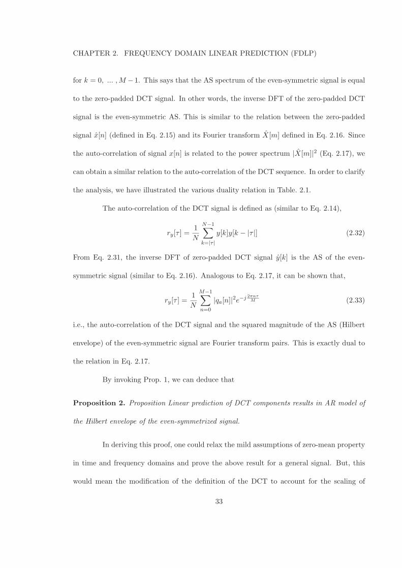
of speech signal, (b) Power spectrum and the TDLP approximation. . . . . 282.3 (a) A portion of speech signal, (b) Spectral AR model (TDLP) and (c) Tem-
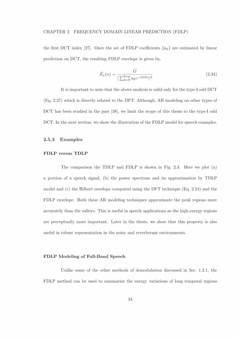
poral AR model (FDLP). . . . . . . . . . . . . . . . . . . . . . . . . . . . . 352.4 Illustration of the AR modeling property of FDLP. (a) a portion of speech
signal, (b) its Hilbert envelope and (c) all pole model obtained using FDLP. 362.5 Illustration of AM-FM decomposition using FDLP. (a) a portion of band pass
filtered speech signal, (b) its AM envelope estimated as square root of FDLPenvelope and (c) the FDLP residual containing the FM component. . . . . . 37
2.6 Plot of 125 ms of input signal in time domain (a), (c) and the correspondinglog FDLP envelopes (b), (d). . . . . . . . . . . . . . . . . . . . . . . . . . . 38
2.7 Normalized resolution in FDLP as function of the location of the first peakfor a 125 ms long signal. (a) Two LP methods, (b) Various DCT windows,(c) FDLP model order and (d) symmetric padding at the boundaries. . . . 40
2.8 Log FDLP envelopes from clean and noisy (babble at 10 dB) sub-band speech.(a) Low resolution envelopes and (b) High resolution envelopes. . . . . . . . 42
3.1 (a) Spectrum of a clean speech envelope for a narrow-band signal (b) Spec-trum of a typical room-response envelope for a narrow-band signal (smalldynamic range). . . . . . . . . . . . . . . . . . . . . . . . . . . . . . . . . . . 52
3.2 (a) Spectrum of a clean speech envelope for a wide-band decomposition (b)Spectrum of a typical room-response envelope for a wide-band decomposition(large dynamic range compared to Fig. 3.1 (b)). . . . . . . . . . . . . . . . . 53
3.3 Summary of the assumptions made for reverberant signal. The effect appearsas a modification of the gain of the sub-band FDLP model in narrow bands. 54
xiii
LIST OF FIGURES
3.4 Log FDLP envelopes for clean and reverberant speech for sub-band 750−850Hz. (a) without gain normalization (b) with gain normalization. . . . . . . 56
3.5 Log FDLP envelopes for clean and telephone speech for sub-band 750− 850Hz. (a) without gain normalization (b) with gain normalization. . . . . . . 57
4.1 Block schematic for the deriving sub-band Hilbert envelopes using FDLP. . 614.2 An experimental signal with impulsive nature in time-frequency domain used
for the resolution analysis of FDLP spectrogram. . . . . . . . . . . . . . . . 634.3 FDLP spectrogram for the signal in Fig. 4.2 using 120 sub-bands and FDLP
model order of 20 poles per sub-band per second. . . . . . . . . . . . . . . . 634.4 FDLP envelope of the sub-band around 2 kHz for the signal in Fig. 4.2 with
a FDLP model order of 20 poles per second. . . . . . . . . . . . . . . . . . . 644.5 Comparison of Mel and FDLP spectrogram for a speech signal. FDLP is
applied on 37 Mel-bands. . . . . . . . . . . . . . . . . . . . . . . . . . . . . 654.6 FDLP Short-term (FDLP-S) Feature Extraction Scheme. . . . . . . . . . . 664.7 Comparison of CMS for MFCC and gain normalization for FDLP. . . . . . 684.8 Recognition accuracy as function of the number of sub-bands. . . . . . . . . 724.9 Word recognition accuracy as function of the bandwidth of the sub-band for
clean and two types of reverberant data. . . . . . . . . . . . . . . . . . . . . 734.10 Word recognition accuracy as function of the model order for clean and two
types of reverberant data. The best performance in each condition is high-lighted using the star sign. . . . . . . . . . . . . . . . . . . . . . . . . . . . . 74
4.11 Word recognition accuracy as function of the expansion factor for clean andtwo types of reverberant data. . . . . . . . . . . . . . . . . . . . . . . . . . . 75
4.12 Comparison of word recognition accuracies (%) using different techniquesusing 6 artificial room responses. . . . . . . . . . . . . . . . . . . . . . . . . 77
5.1 Block schematic for the FDLP based modulation feature extraction usingstatic and dynamic compression. . . . . . . . . . . . . . . . . . . . . . . . . 86
5.2 Dynamic compression of the sub-band FDLP envelopes using adaptive com-pression loops. . . . . . . . . . . . . . . . . . . . . . . . . . . . . . . . . . . 87
5.3 Static and dynamic compression of the temporal envelopes: (a) a portionof 1000 ms of full-band speech signal, (b) the temporal envelope extractedusing the Hilbert transform, (c) the FDLP envelope, which is an all-poleapproximation to (b) estimated using FDLP, (d) logarithmic compression ofthe FDLP envelope and (e) adaptive compression of the FDLP envelope. . . 88
5.4 Block schematic for noise compensation in FDLP. . . . . . . . . . . . . . . . 975.5 Gain normalized sub-band FDLP envelopes for clean and noisy speech signal
(babble 10 dB) (a) without and (b) with MMSE noise suppression. . . . . . 99
6.1 Scheme of the FDLP encoder. . . . . . . . . . . . . . . . . . . . . . . . . . . 1146.2 Scheme of the FDLP Decoder. . . . . . . . . . . . . . . . . . . . . . . . . . 1146.3 Application of temporal masking to reduce the bits for 200ms region of a sub-
band signal. The figure shows the temporal masking threshold, quantizationnoise for the codec without and with temporal masking. . . . . . . . . . . . 120
xiv
LIST OF FIGURES
6.4 Sub-band processing in FDLP codec with SNS. . . . . . . . . . . . . . . . . 1226.5 Improvements in reconstruction signal quality with SNS: A portion of power
spectrum of (a) a tonal input signal, (b) reconstructed signal using the base-line FDLP codec without SNS, and (c) reconstructed signal using the FDLPcodec with SNS. . . . . . . . . . . . . . . . . . . . . . . . . . . . . . . . . . 123
6.6 MUSHRA results for each audio sample type namely speech, mixed and mu-sic content obtained using three coded versions at 48 kbps (FDLP-MDCT(FDLP), MPEG-4 HE-AAC (AAC) and LAME-MP3 (LAME)), hidden ref-erence (Hid. Ref.) and 7 kHz low-pass filtered anchor (LPF7k) with 8 listeners.127
7.1 Block schematic of 2-D AR model based feature extraction. . . . . . . . . . 138
C.1 Wide-band STFT spectrogram for the signal in Fig. 4.2 using 25 ms windowwith half overlap. . . . . . . . . . . . . . . . . . . . . . . . . . . . . . . . . . 150
C.2 Narrow-band STFT spectrogram for the signal in Fig. 4.2 using 200 ms win-dow with half overlap. . . . . . . . . . . . . . . . . . . . . . . . . . . . . . . 151
xv
Chapter 1
Introduction
1.1 Motivation
1.1.1 Conventional Signal Analysis
Typically, a speech/audio processing system has a front-end signal analysis stage which
receives its input as a sequence of signal samples and converts it into a representation
which is suitable for further processing. The main function of this analysis block is to
preserve necessary signal information in a compact manner while suppressing irrelevant
redundancies.
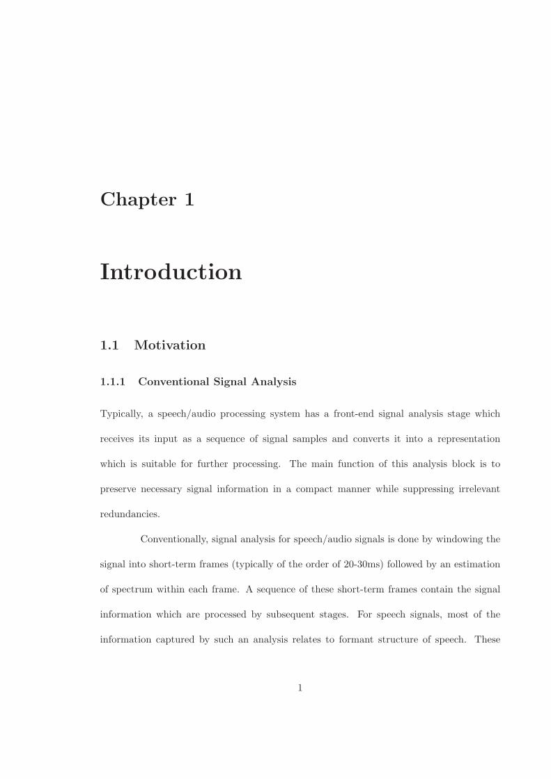
Conventionally, signal analysis for speech/audio signals is done by windowing the
signal into short-term frames (typically of the order of 20-30ms) followed by an estimation
of spectrum within each frame. A sequence of these short-term frames contain the signal
information which are processed by subsequent stages. For speech signals, most of the
information captured by such an analysis relates to formant structure of speech. These
1
CHAPTER 1. INTRODUCTION
(a) (b)
Processing
frame
Processing frame
Time
Fre
quen
cy
Time
Fre
quen
cy
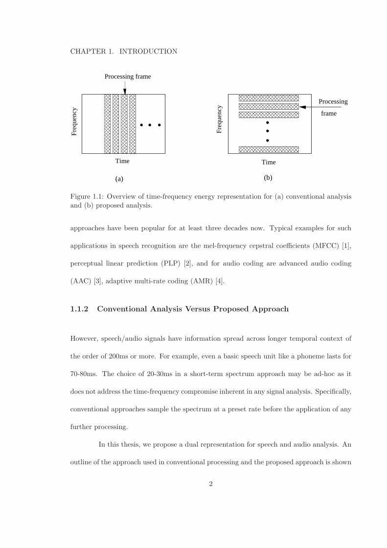
Figure 1.1: Overview of time-frequency energy representation for (a) conventional analysisand (b) proposed analysis.
approaches have been popular for at least three decades now. Typical examples for such
applications in speech recognition are the mel-frequency cepstral coefficients (MFCC) [1],
perceptual linear prediction (PLP) [2], and for audio coding are advanced audio coding
(AAC) [3], adaptive multi-rate coding (AMR) [4].
1.1.2 Conventional Analysis Versus Proposed Approach
However, speech/audio signals have information spread across longer temporal context of
the order of 200ms or more. For example, even a basic speech unit like a phoneme lasts for
70-80ms. The choice of 20-30ms in a short-term spectrum approach may be ad-hoc as it
does not address the time-frequency compromise inherent in any signal analysis. Specifically,
conventional approaches sample the spectrum at a preset rate before the application of any
further processing.
In this thesis, we propose a dual representation for speech and audio analysis. An
outline of the approach used in conventional processing and the proposed approach is shown
2
CHAPTER 1. INTRODUCTION
in Fig. 1.1. In the conventional approach, an individual processing frame is a short-term
spectrum estimated on the signal. This is shown in Fig. 1.1(a). The individual spectral
frames are stacked in a column-wise manner to obtain a two-dimensional (2-D) representa-
tion of the speech signal. An alternate way to construct the same 2-D representation is to
process a single frequency band over a long duration and stack these bands in a row-wise
manner. This is shown in Fig. 1.1(b). This processing technique is dual to conventional
methods and therefore opens a variety of applications. From a historical perspective, the
proposed method of signal analysis comes from the underlying principle of sound spectro-
graph which was widely used for speech and audio analysis in 1950s [5]. In operation, the
sound is stored in magnetic/metal disk and it is played many times. In each repetition,
the signal is passed is through a band-pass filter whose frequency range is varied in each
repetition. The output of the filter is recorded in a paper placed on a rotating drum. The
amplitude fluctuations are recorded as intensity variations on the paper - darker regions
corresponding to higher energy levels. After each repetition the stylus is shifted so at to
represent the next frequency range. By this process, a 2-D representation of the sound is
produced. This method is fundamentally similar to the proposed scheme in Fig. 1.1(b).
The modulation spectrum is defined as the spectral transform of the amplitude
modulation of the speech signal in sub-bands. In Sec. 1.2.1, we describe various ways of
estimating the amplitude modulation. The modulation spectrum for speech signal has a
typical shape with a peak activity around 4 Hz for speech signals.
There has been various studies in the past two decades providing physiological
and psycho-physical evidences for existence of a modulation representation in the human
3
CHAPTER 1. INTRODUCTION
auditory system. Although a number of examples can be cited in this regard, we limit the
discussion to a few important cases.
Physiological Evidence
Spectro-Temporal Receptive Field (STRF) - Various studies have been done on
analyzing the front-end cochlear processing in the human auditory system. These
studies have also made significant influence in automatic speech recognition and coding
(for example, the use of critical bandwidth in perceptual linear prediction (PLP)
processing [2]). Recently, several studies have also tried to unravel the signal analysis
involved in higher levels of auditory processing like the primary auditory cortex [6].
Specifically, much insight about the physiological functions can be gained by the
measuring the spectro-temporal receptive fields (STRFs) of the auditory neurons in
the cortex of animals and humans. The STRF denotes a two dimensional time-
frequency impulse response of a neuron assuming a linear model for the neuron and
determines the modulation selectivity of the neuron. In the scope of this thesis, the
most relevant aspect of STRFs is the temporal span of these measured responses.
Typically, some of these STRFs extend for about 250 ms or more [6] which is about a
syllable length in speech signals. If we desire to have a signal analysis scheme which
is consistent with these physiological studies, there is a need to process longer context
of speech/audio signals than the conventional 25ms.
Psychophysical Evidence
4
CHAPTER 1. INTRODUCTION
Importance of modulation frequency selectivity - The importance of various mod-
ulation frequencies in speech has been analyzed using a set of psychophysical exper-
iments [7, 8]. In the first set of experiments, speech envelope in sub-bands (octave
bands) is downsampled and filtered using a low-pass filter with a variable cut-off
frequency [7]. The ratio of filtered envelope to the original envelope is used as a
modulation function on the original sub-band signal. Finally, a sub-band re-synthesis
is done to obtain a full-band speech signal. The modified speech signal is used for
listening experiments on a sentence recognition as well as a phoneme recognition task.
By varying the cut-off frequency of the filter, the effect of removing the lower and
higher modulations is analyzed. The results from these two experiments indicate that
most of the speech intelligibly is contained in 1 − 16 Hz of modulations with a peak
sensitivity at 4 Hz. In order to extract relevant modulation information from a speech
signal, the analysis window must be long enough (for example, a window length of
250 ms is needed for representing a 4 Hz modulation component).
Filtering of cepstral coefficients - Since cepstral coefficients are widely used in speech
recognition applications, the effect of band-pass filtering of cepstral coefficients for
speech intelligibility was studied in [9]. In these studies, LP parameters are estimated
in short-term frames and are converted to cepstral coefficients. The sequence of cep-
stral coefficients are then filtered using a low-pass, high-pass and band-pass filter.
The filtered cepstral coefficients are converted back to the LP parameters which are
used to filter the original LP residual. The results of these experiments suggest that
speech intelligibility is not degraded when the cut-off frequency for the low-pass filter
5
CHAPTER 1. INTRODUCTION
is above 24 Hz, Similarly, intelligibility is also preserved when the cut-off frequency
for the high-pass filter is below 1 Hz [9]. These results are similar to experiments done
in [7].
Spectral versus temporal modulation - An investigation on the relative importance
of the spectral versus temporal modulation was done with human speech recogni-
tion experiments in [10]. Specifically, the experiment was designed to determine the
lower limit on the number of spectral bands required for nearly perfect human speech
recognition. Speech signal was analyzed in a set of broad frequency bands and the en-
velope information was extracted using a half-wave rectifier and low-pass filter. This
envelope was used to modulate white noise with the same band-width as the original
speech sub-band. These sub-bands were re-synthesized to form a full-band signal and
listening experiments were conducted using these signals for sentence and phoneme
recognition. The variable parameter is the number of broad sub-bands used to derive
the envelope information. The result of these experiments [10] suggest that good hu-
man speech recognition performance can be obtained with only 3-4 sub-bands as long
as the temporal modulation cues are well preserved.
1.2 Past Modulation Approaches
Modulation analysis of speech/audio signal refers to the method of decomposing sub-band
speech signal as a multiplication of a slowly varying envelope signal with a fine carrier signal.
The smooth modulating signal, referred to as the amplitude modulation (AM) component,
summarizes the energy variation as a function of time for the particular sub-band. The
6
CHAPTER 1. INTRODUCTION
carrier signal, referred to as the frequency modulation (FM) component tries to capture the
fine frequency variations around the center frequency of the sub-band. The carrier signal
does not contain significant energy variations as these are captured by the AM component.
Such an AM-FM decomposition performed over all sub-bands constitutes a signal analysis
technique for speech/audio signals.
In the past, several techniques have been proposed for deriving sub-band modu-
lations in speech/audio processing systems. In this section, we review some of the popular
techniques and their applications.
1.2.1 Demodulation Methodologies
Half-wave Rectification
One of the earliest methods of deriving the envelope from an amplitude modulated signal
is that of half-wave rectification with a low-pass filter [11]. In an analog circuitry, this can
be implemented using a diode and an integrator. Moreover, there is physiological evidence
for the half-wave rectification in the inner hair cells of cochlea. The design of the cut-off
frequency1 for the low-pass filter is critical for this method of AM detection. A lower value
for the cut-off frequency will result in loss of important signal information where as a higher
cut-off frequency will result in additional noise in the signal.
Hilbert Envelope
The analytic signal representation of a real-valued signal is the sum of the signal and its
quadrature component [12]. Let x(t) denote a time domain signal. Its analytic signal, as
1The cut-off frequency is typically chosen based on prior information about the modulation extent
7
CHAPTER 1. INTRODUCTION
defined by Gabor [12], can be written as,
xa(t) = x(t) + jH[
x(t)]
, (1.1)
where H denotes Hilbert transform operator which is a convolution of the signal2 with
1πt
[13]. The Hilbert envelope is defined as the squared magnitude of the analytic signal.
Ex(t) = |xa(t)|2, (1.2)
The analytic signal has one-sided spectrum (non-zero only for positive frequencies). The
Hilbert envelope can be shown to be the squared AM envelope for band-limited modulated
signals [14, 15]. Thus, extraction of the Hilbert envelope results in the AM detection.
Short-term Spectral Energy
The evolution of the short-term spectral energy in individual sub-bands can be used as
representation of the modulations in individual sub-bands [16]. The signal is framed using
short-term (20 − 30ms) windows and the magnitude of the Fourier transform is computed
in each frame (short-term Fourier transform (STFT)). Specifically, let
S(ω, t) = F[
x(τ)w(τ − t)]
(1.3)
denote the STFT. For a particular frequency ωk, |S(ωk, t)|2 represents a time domain func-
tion of the evolution of spectral energy. A Fourier transform of this function can yield the
modulation spectrum of speech [16].
2This is shown in Appendix A.1
8
CHAPTER 1. INTRODUCTION
Teager Energy Operator
The Teager energy operator is defined as [17]
ψ[
x(t)]
=∂x(t)
∂t− x(t)
∂2x(t)
∂t2(1.4)
For an AM-FM signal,
x(t) = a(t)cos[φ(t)], (1.5)
it can be shown that the AM signal magnitude can be obtained as [18]
|a(t)| = ψ[
x(t)]
√
ψ[∂x(t)
∂t
]
(1.6)
This method is referred to as the energy separation algorithm (ESA) and can be applied
for AM-FM decomposition of speech and audio signals.
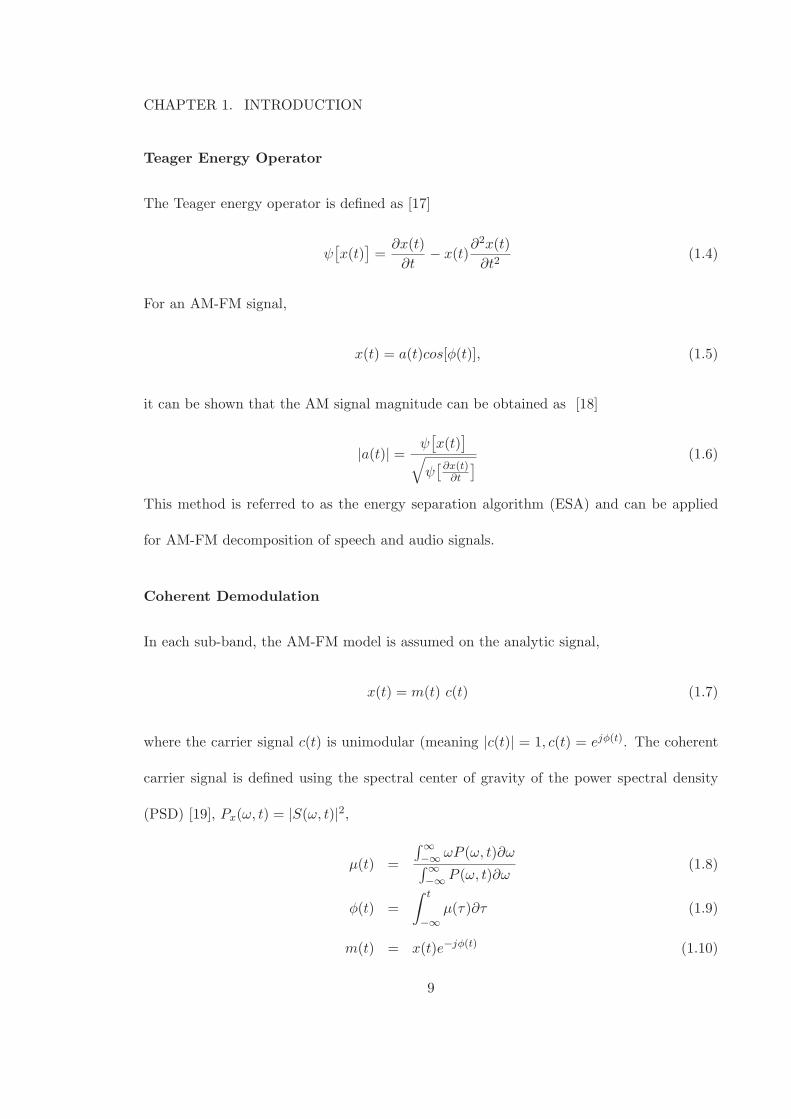
Coherent Demodulation
In each sub-band, the AM-FM model is assumed on the analytic signal,
x(t) = m(t) c(t) (1.7)
where the carrier signal c(t) is unimodular (meaning |c(t)| = 1, c(t) = ejφ(t). The coherent
carrier signal is defined using the spectral center of gravity of the power spectral density
(PSD) [19], Px(ω, t) = |S(ω, t)|2,
µ(t) =
∫∞−∞ ωP (ω, t)∂ω∫∞−∞ P (ω, t)∂ω
(1.8)
φ(t) =
∫ t
−∞µ(τ)∂τ (1.9)
m(t) = x(t)e−jφ(t) (1.10)
9
CHAPTER 1. INTRODUCTION
In this case, the modulating signal is complex unlike the previous methods. In [19], the
authors argue that the choice of complex modulating signal and carrier ensures that for a
bandlimited signal, the envelope and the carrier are also bandlimited.
1.2.2 Applications of Past Approaches
Speech Transmission Index (STI)
One of the earliest applications of the modulation spectrum is the concept of speech trans-
mission index (STI) [20]. STI is used to predict the intelligibility of reverberated signal
in room acoustics. For this purpose, input speech signal x(t) is recorded using a far-field
microphone y(t) and an objective score is derived using the modulation transfer function
(MTF). MTF is defined as the ratio of the magnitude modulation spectrum of output to
that of the input. Let Ex(t), Ey(t) be temporal envelope of input and the output and Ex(f),
Ey(f) denote the corresponding modulation spectra. MTF is defined as,
MTF = α|Ey(f)||Ex(f)|
(1.11)
where α is a normalization constant based on the mean value of Ex(t) and Ey(t). In each
sub-band, the MTF is computed on 14 modulation frequencies from 0.63 Hz to 12.5 Hz
with one-third octave frequency spacing for each of the 7 audio frequency sub-bands which
are octave spaced [20]. The MTF is converted to a signal-to-noise ratio using,
S/N = 10 log10
[
MTF
(1−MTF )
]
(1.12)
The average S/N computed over the matrix of 14 × 7 MTF values is used as the speech
intelligibility measure. This measure is also shown to have good correlation with subjective
10
CHAPTER 1. INTRODUCTION
tests performed using reverberated data [20].
Enhanced Spectral Dynamics
The first application of modulation filtering for feature extraction of speech recognition is
the use of derivative features [21]. Cepstral coefficients from short-term frames are extracted
and a context of 7 frames is used for a cepstral filtering process with pre-defined polynomial
coefficients. This filtering yield first and second derivatives of cepstral coefficients. These
are linearly related to the derivative and double derivatives of the log-spectrum of the speech
signal [21]. The derivative features are the output of a band-pass modulation filtering where
the 0 Hz component is removed. These delta cepstral coefficients are linearly combined with
the direct cepstral coefficients and are used for speech recognition. In these experiments,
the derivative features reduce the error rate by half [21].
RASTA and M-RASTA Processing
Relative spectra (RASTA) [16] is method of feature extraction for speech recognition which
tries to achieve robustness to channel distortions using principles of modulation spectra.
As discussed in Sec. 1.1.2, the important speech information for human perceptual system
lies in 1 − 16 Hz of modulations. Some of the temporal effects introduced by the channel
artifacts lie outside this region of the modulation spectrum. By means of band-pass filtering,
the modulations relevant to the speech signal can alone be preserved and those pertaining
to the channel artifacts can be removed. This is particularly useful in automatic speech
recognition (ASR) in mis-matched channel conditions [16], where the channel effects are
convolutive in the signal domain and appear as additive component in the log-spectral
11
CHAPTER 1. INTRODUCTION
domain. Modulation processing for RASTA is done using the short-term critical band
energy representations (Sec. 1.2.1).
In an extension of the RASTA approach, called the MRASTA technique, a bank of
multi-resolution band-pass filters are applied on spectrographic representation of speech [22].
These filters try to emulate the multi-resolution processing performed in the higher stages
of the human auditory processing. A context of 1s is used in these filters and all the
MRASTA filters have the zero mean property which ensures the removal of convolutive
channel artifacts. Significant improvements can be obtained in telephone channel speech
recognition using the MRASTA technique [22].
Modulation Spectrogram
Modulation spectrogram (MSG) [23] refers to a front-end representation for speech signals
derived from filtered trajectories of sub-band AM envelopes. These envelopes are derived
using the half-wave rectification based demodulation methodology (Sec. 1.2.1). The sub-
band envelopes are normalized with a long-term average, down-sampled and low-pass filtered
in the 0 − 8 Hz range with a complex filter. The log-magnitude output of this filter are
used to obtain features. In speech recognition experiments, the MSG front-end provides
good improvements for reverberant data. It also works well in combination with RASTA
processing.
Source Separation
Coherent demodulation provides complex estimates of modulation signal which can be used
for modulation filtering to separate music signals [24]. In this method, a low-pass filter is
12
CHAPTER 1. INTRODUCTION
used in the coherent AM signal to separate a flute signal from a castanet signal. Such an
approach has also been extended to separation of overlapped speech [25].
1.2.3 Comments on Past Methodologies
Although a number of approaches have been proposed in the past for deriving modulation
representation of speech/audio signals, most of these approaches have shown to be promising
for a limited set of applications. The applicability could not be extended beyond these tasks
where the short-term spectral approaches continue to remain popular. This is partly due
to the following reason.
The underlying mathematical model defining the AM-FM model is an approxi-
mation under certain assumptions of the modulation/carrier signal which are easily vio-
lated. These properties include basic requirements like linearity and continuity [15]. For
example, the application of demodulation using Teager energy based demodulation yields
unreasonable AM components for wide-band signals [15]. The assumptions of complex rep-
resentation of modulating signal for coherent demodulation is unrealistic for natural signals
like speech/audio. The only methodology which satisfies the linearity and homogeneity
properties is the Hilbert envelope (discussed in detail in Chap. 2). Thus, in this thesis,
we focus on the modeling of the Hilbert envelope using frequency domain linear prediction
(FDLP) [26,27].
13
CHAPTER 1. INTRODUCTION
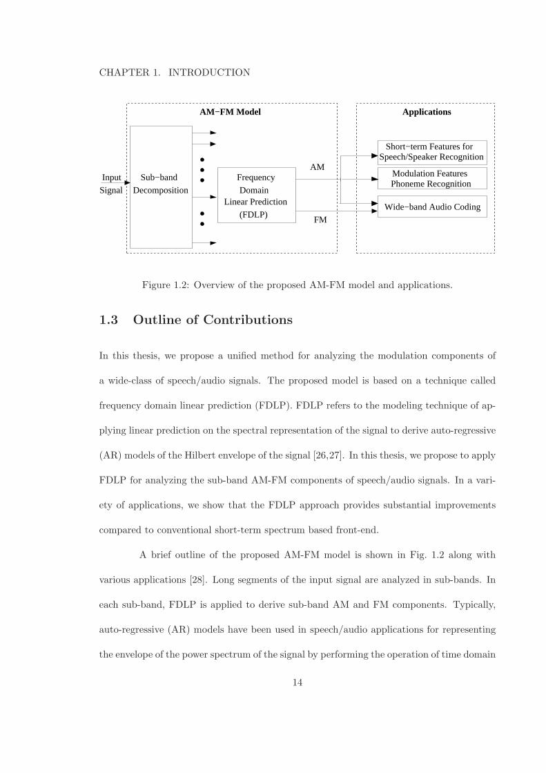
AM−FM Model Applications
AMFrequency
DomainLinear Prediction
(FDLP)
Decomposition
Sub−band
FM
Short−term Features forSpeech/Speaker Recognition
Modulation FeaturesPhoneme Recognition
Wide−band Audio Coding
Signal
Input
Figure 1.2: Overview of the proposed AM-FM model and applications.
1.3 Outline of Contributions
In this thesis, we propose a unified method for analyzing the modulation components of
a wide-class of speech/audio signals. The proposed model is based on a technique called
frequency domain linear prediction (FDLP). FDLP refers to the modeling technique of ap-
plying linear prediction on the spectral representation of the signal to derive auto-regressive
(AR) models of the Hilbert envelope of the signal [26,27]. In this thesis, we propose to apply
FDLP for analyzing the sub-band AM-FM components of speech/audio signals. In a vari-
ety of applications, we show that the FDLP approach provides substantial improvements
compared to conventional short-term spectrum based front-end.
A brief outline of the proposed AM-FM model is shown in Fig. 1.2 along with
various applications [28]. Long segments of the input signal are analyzed in sub-bands. In
each sub-band, FDLP is applied to derive sub-band AM and FM components. Typically,
auto-regressive (AR) models have been used in speech/audio applications for representing
the envelope of the power spectrum of the signal by performing the operation of time domain
14
CHAPTER 1. INTRODUCTION
linear prediction (TDLP) [29]. This thesis utilizes AR models for obtaining smoothed,
minimum phase, parametric models of temporal envelopes. For the FDLP technique, the
squared magnitude response of the all-pole filter approximates the Hilbert envelope of the
signal (in a manner similar to the approximation of the power spectrum of the signal by
TDLP [29]).
The all-pole parameters of FDLP provide the AM signal and the residual (cor-
responding to the LP error signal in the frequency domain) of the FDLP constitutes the
FM component (carrier). The AM part carries the “message” information of the signal
and is used for speech and speaker recognition applications. In this regard, we develop two
different feature extraction methods -
1. Short-term features obtained by integrating the FDLP envelopes in short-time win-
dows. These are similar to conventional MFCC features.
2. Modulation features which are obtained from syllable length windows (200 ms) of
sub-band envelopes. These features are high dimensional and are useful in phoneme
recognition tasks.
The FM components carry information about the fine structure of the sub-band signal and
enhance the quality of the signal. These are useful in high quality wide-band audio coding
applications where the goal is to preserve the reconstruction quality.
1.4 Road Map for Rest of the Thesis
The organization of various chapters in this thesis is shown in Fig. 1.3. The rest of the
thesis is organized as follows. Chap. 2 describes the FDLP model in detail. It begins
15

CHAPTER 1. INTRODUCTION
Chap. 3
Chap. 4Short−term
Features
Chap. 5
FeaturesModulation
Audio Coding
Chap. 6Gain Norm.
Chap. 7
Extensions
Chap. 2
FDLP
Chap. 1Outline
Figure 1.3: Connections among various chapters in this thesis.
with a overview of the past literature on AR modeling of Hilbert envelopes. Then, the
underlying mathematical model of FDLP is developed where we prove the fundamental
result - Application of linear prediction on the DCT of the signal gives an AR
model of the Hilbert envelope of the signal [27]. This proof is derived by the
application of duality concepts to conventional TDLP [29] and is done in discrete signal
domain. We illustrate the AM-FM decomposition properties of FDLP on synthetic as well
as natural signals. The resolution of FDLP modeling is analyzed and the choice of model
order is also discussed.
In Chap. 3, we propose the gain normalization technique for FDLP. We begin with
the discussion of the issue of reverberation in speech processing systems. Then, the gain
normalization procedure is explained which provides robustness to the FDLP representation
in noisy and reverberant environments. The underlying assumption in gain normalization
and its usefulness are analyzed in detail. We use the gain normalization on the FDLP en-
16
CHAPTER 1. INTRODUCTION
velopes for speech recognition applications as it provides good robustness without reducing
the performance in clean conditions.
Chap. 4 outlines the speech and speaker recognition experiments using short-term
FDLP features. Speech recognition experiments in mismatched training and test conditions
are also discussed here. In all these experiments, the back-end speech recognition system
is based on Hidden Markov Model-Gaussian Mixture Model (HMM-GMM). These experi-
ments highlight the importance of gain normalization of FDLP envelopes. We also compare
the performance of the proposed features with other robust features extraction techniques
proposed in the past. Speaker recognition experiments are done in matched conditions using
telephone and far-field microphone data.
Modulation features derived from long-term trajectories of FDLP envelopes are dis-
cussed in Chap. 5. We propose a combination of static and dynamic modulation frequency
features for phoneme recognition. We also develop the noise compensation technique for
FDLP envelopes, which tries to provide robustness in additive noise scenarios. These fea-
tures are used in the hybrid hidden Markov model - artificial neural network (HMM-ANN)
system. Experiments are performed in mis-matched train/test conditions where the test
data is corrupted with various environmental distortions like telephone channel noise, ad-
ditive noise and room reverberation. Experiments are also performed on large amounts of
real conversational telephone speech. Furthermore, the contribution of various processing
stages for robust speech signal representation is analyzed.
Audio coding using FDLP technique is described in Chap. 6. We propose a simple
audio-codec which can provide good reconstruction quality for a wide-class of speech and
17
CHAPTER 1. INTRODUCTION
audio signals with a bit-rate ranging from 32-64 kbps. We also utilize novel aspects of
temporal masking and spectral noise shaping to improve the performance of the FDLP
codec. The chapter ends with a discussion of the subjective and objective quality evaluations
which compare the FDLP codec with other state-of-the-art speech/audio codecs.
In Chap. 7, future directions and extensions of the FDLP methodology are men-
tioned. The application of FDLP modulation features for speaker recognition is investigated
in detail. In the last part of the chapter, we analyze the fundamental limits and shortcom-
ings of FDLP approach. This would determine the range of applicability of FDLP technique
for speech/audio systems. This chapter also provides a brief summary of the various con-
tributions of this thesis.
18
Chapter 2
Frequency Domain Linear
Prediction (FDLP)
2.1 Chapter Outline
In this chapter, we describe the underlying mathematical model of frequency domain linear
prediction (FDLP). We begin by highlighting the properties of analytic signal which make
it an important method for demodulation (Sec. 2.2). Then, we review the past approaches
for AR modeling of Hilbert envelopes (Sec. 2.3). Some relevant details of conventional linear
prediction are reviewed next (Sec. 2.4). This is followed by the extension of conventional
linear prediction to FDLP (Sec. 2.5). We illustrate the AM-FM decomposition of FDLP
using full-band as well as sub-band speech signals (Sec. 2.5.3). The chapter ends with a
discussion of the temporal resolution of the FDLP model and its interaction with the model
order (Sec. 2.6).
19
CHAPTER 2. FREQUENCY DOMAIN LINEAR PREDICTION (FDLP)
+
H
| | a(t)
jx(t)ddt
φ (t)
ω (t)
Figure 2.1: Demodulation procedure using analytic signal.
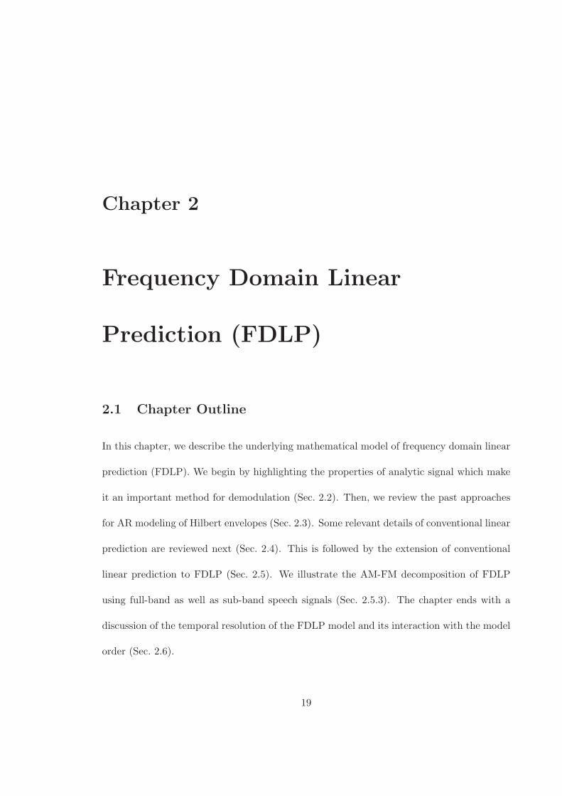
2.2 Properties of Analytic signal
In this section, we show some of the useful properties of continuous analytic signal (AS).
We follow the notation used in [15]. Let x(t) denote a real signal of the form,
x(t) = m(t)cos[φ(t)], (2.1)
φ(t) = ω0t+Φ(t), (2.2)
where, m(t), φ(t) and ω(t) = dφ(t)dt
are the amplitude, phase and frequency modulation (AM,
PM and FM) respectively. The AS is a complex representation of the real input signal given
by (rewriting Eq. 1.1),
xa(t) = x(t) + jH[
x(t)]
(2.3)
= m(t)ejφ(t) (2.4)
where the Hilbert transform operator H is defined as1,
H[
x(t)]
=1
π
∫ ∞
−∞
x(τ)
t− τdτ (2.5)
1This is derived in Appendix A.1
20
CHAPTER 2. FREQUENCY DOMAIN LINEAR PREDICTION (FDLP)
Now, the amplitude and phase modulation can be obtained as
m(t) = |xa(t)|, (2.6)
φ(t) = arctan
[
Imxa(t)Rexa(t)
]
(2.7)
The demodulation procedure using the analytic signal is outlined in Fig. 2.1. We refer to
this procedure as the AS based demodulation operator.
We can list the desired properties of a well-defined amplitude demodulation oper-
ator. Here, we also show that AS defined in Eq.2.3 satisfies all these properties [15].
1. Amplitude Continuity - In an ideal demodulator, a small variation in the signal
(x(t) → x(t) + δx(t)) should make a small variation in the amplitude modulation
(m(t) → m(t) + δm(t)). This can be guaranteed as the Hilbert transform satisfies,
H[
x(t) + δx(t)]
→ H[
x(t)]
as δ → 0 (2.8)
and the magnitude of the AS which gives the AM (Eq. 2.6).
2. Homogeneity - Scaling the signal (x(t) → cx(t)) should modify only the amplitude
modulation (m(t) → |c|m(t)) and leaves the frequency modulation unchanged. This
is satisfied by the AS because,
H[
cx(t)]
= cH[
x(t)]
(2.9)
3. Harmonic Correspondence - A sinusoid (x(t) = cos(ωt)) should have m(t) = 1 and
φ(t) = ωt. This is also satisfied as,
H[
cos(ωt)]
= sin(ωt), (2.10)
The above relation is derived in Appendix A.3.
21

CHAPTER 2. FREQUENCY DOMAIN LINEAR PREDICTION (FDLP)
In fact, it can be shown that the AS is the unique linear operator which satisfies all these
properties [15]. The demodulation using AS can be achieved using Eq. 2.6. Furthermore,
this demodulation gives reasonable results for wide-band noisy signals which may not be
satisfied by other demodulators [15]. Thus, the AS forms a suitable choice for the represen-
tation of modulation information in speech and audio signals.
However, the computation of the AS involves the computation of the Hilbert trans-
form using the Hilbert operator defined in Eq. 2.5. Note that, the Hilbert transform operator
is a filter with infinite impulse response in both directions. This would lead to a number of
difficulties for a finite duration real-valued signal. For example, this would lead to signifi-
cant transients in the analytic signal and alters the characteristics. Hence, it is desirable to
model the Hilbert envelope without the explicit computation of the Hilbert transform.
2.3 Past Approaches in AR modeling of Hilbert Envelopes
2.3.1 Temporal Noise Shaping (TNS)
In audio coding using spectral domain quantization and coding, the quantization noise
involved in encoding transient signals spreads across the entire analysis window causing
distortions called pre-echo artifacts [30]. Temporal noise shaping (TNS) is a technique by
which the quantization noise at the receiver is shaped according to the input signal so that
the noise gets masked by the input signal. Specifically, the TNS implements D∗PCM [31]
in the spectral domain.
Conventional D∗PCM in the time domain relates to the technique where the pre-
diction error of a signal is quantized and transmitted instead of the original signal. In the
22
CHAPTER 2. FREQUENCY DOMAIN LINEAR PREDICTION (FDLP)
decoder, the quantization noise is filtered with the inverse LP filter which shapes the quan-
tization noise in spectral domain according to the input signal. Combining this observation
with the time-frequency duality, we can conclude that the application of predictive coding
to spectral data over frequency can shape the the quantization error according to be the
temporal shape of the input signal [30]. The inverse filter response in this case is the Hilbert
envelope of the signal.
2.3.2 Linear Prediction in Spectral Domain (LPSD)
A periodic continuous-time band-limited AS xa(t) with a period T and fundamental fre-
quency Ω = 2πT
can be expanded using the Fourier series as [32]
xa(t) = ejω0tM∑
k=0
ckejkΩt (2.11)
where ω0 represents a frequency translation in order to make summation index between
0 and M . The above expression can be regarded as a polynomial in complex time plane
and the roots of the polynomial can be sorted to those inside the unit circle (equivalent
to minimum phase spectral representation) and those outside the unit circle (equivalent to
maximum phase spectral representation).
xa(t) = a0ejω0t
P∏
i=1
(1− piejΩt)
Q∏
i=1
(1− qiejΩt) (2.12)
where the complex roots |pi| < 1 and |qi| > 1 and P +Q =M . We have also assumed that
none of the zeros fall on the unit circle. The above equation shows that a complex time
domain signal can be split into a minimum-phase, maximum-phase product form (similar to
spectral decomposition of signals into minimum-phase and maximum-phase components).
Further, the minimum-phase component can be modeled using a linear prediction approach.
23
CHAPTER 2. FREQUENCY DOMAIN LINEAR PREDICTION (FDLP)
For a non-periodic signal observed in a window of finite duration T , the above
expansion can be applied assuming a infinite periodic extension of the signal. Without
trying to root the polynomial for finding the minimum phase component, a linear prediction
model h(t) can be computed which minimizes the energy of error function (e(t)) [26, 33]
∫ T
0|e(t)|2dt =
∫ T
0|xa(t)|2|h(t)|2dt (2.13)
where h(t) = 1 +∑p
k=1 hkejkΩt. This method is analogous to conventional time domain
linear prediction [29] but the parameters hk are estimated as the prediction coefficients
of the Fourier transform of the signal. For a discrete time signal, the coefficients hk can
be estimated in closed form using a set of p equations in p unknowns [26]. The Hilbert
envelope of the signal is obtained as the squared inverse signal response in the time-domain
1|h(t)|2 . This method results in a prediction error e(t) which is maximum phase signal and
can be applied for AM-FM decomposition of filtered speech signals.
2.3.3 AR Modeling of Temporal Envelopes
The connection between the linear prediction in DCT domain and AR modeling of discrete
time AS is established in [27, 34]. This is an extension of LPSD approach using discrete-
time version of the AS. Strictly speaking, an AS cannot be defined for a discrete signal
as the spectrum is periodic. However, by limiting the spectrum to positive frequencies in
[−π, π] range, we can define a discrete version of the AS [35]. The squared magnitude of
the discrete AS (Hilbert envelope) can be approximated using a linear prediction on the
DCT components of a signal. This method is named as frequency domain linear prediction
(FDLP). The FDLP method forms the basis for our thesis and we derive some of the
24
CHAPTER 2. FREQUENCY DOMAIN LINEAR PREDICTION (FDLP)
relations in the underlying model in Sec. 2.5.
An extension of this approach was proposed for feature extraction of speech called
LP-TRAPS [36]. Here, the AR model of Hilbert envelopes is computed in bark-sized sub-
bands with a context of 1s. The LP coefficients are converted to temporal cepstra in each
band and used to train a TRAP TANDEM system [36].
2.4 Linear Prediction
In signal processing theory, time and frequency are two types of dimensions for
expressing the information in the signal. One can shift between these two domains using the
Fourier transform. Duality is defined as the phenomenon for describing the properties which
are identical in time and frequency domains. For example, using the Parseval’s theorem, it
can be shown that the sum of the squared magnitude in two domains are the same.
In the case of linear prediction, we first show that linear prediction in time-domain
estimates the AR model of power-spectrum of the signal. Then, we invoke duality properties
to extend the application of linear prediction in the frequency domain.
2.4.1 Time Domain Linear Prediction (TDLP)
In this section, we review some of the mathematical relations underlying the conventional
time domain linear prediction. We begin the signal processing relations between the auto-
correlation of the signal and power spectral density. Then, we write the linear prediction
model in the time domain and provide a filter interpretation of the optimization involved.
Some of these relations are stated without proof. More details including mathematical
25
CHAPTER 2. FREQUENCY DOMAIN LINEAR PREDICTION (FDLP)
derivations can be found in [29, 37].
Auto-correlation and Power Spectrum
Let x[n] denote a discrete time signal for a finite window of length N . Let rx[τ ] denote the
auto-correlation sequence with lag τ ranging from −N + 1, ..., N − 1 defined as,
rx[τ ] =1
N
N−1∑
n=|τ |x[n]x[n− |τ |] (2.14)
Note that rx[τ ] represents a biased estimator of the auto-correlation. Let x[n] denote the
zero-padded input signal,
x[n] =
x[n] for n = 0 , .., N − 1
0 for n = N, ... ,M − 1
(2.15)
and M = 2N − 1. Then, X[m] denoting M point DFT sequence is,
X[m] =N−1∑
n=0
x[n]e−j 2πnmM (2.16)
for m = 0, ..., M − 1. It can be shown that auto-correlation sequence rx[τ ] is the inverse
DFT of the power spectral density Px[m] = |X[m]|2, i.e.,
rx[τ ] =1
N
M−1∑
m=0
|X[m]|2ej 2πmτM (2.17)
for τ ranging from 0, ..., N − 1 and rx[−τ ] = rx[τ ] for rest of the values of τ .
LP Problem Definition
The time domain linear prediction problem can be stated as follows - The goal is to identify
the set of coefficients ak, k = 1, ... , p such that error signal e[n] defined as
e[n] = x[n]−p
∑
k=1
akx[n− k] (2.18)
26
CHAPTER 2. FREQUENCY DOMAIN LINEAR PREDICTION (FDLP)
has minimal energy Ep =∑N−1
n=0 |e[n]|2.
Multiplying both sides of Eq. 2.18 by x[n − τ ] and summing it over n, we get
(assuming signal values are 0 outside the observation interval)
rx[τ ] =
p∑
k=1
akrx[τ − k], for τ = 1, .. , p (2.19)
G = Ep = rx[0]−p
∑
k=1
akrx[k]. (2.20)
These equations are called Yule-Walker equations and these can be solved in a closed form
to yield the set of predictor coefficients ak .
Filter Interpretation
Let the sequence d[k] be defined as d[0] = 1, d[k] = −ak. Then, Eq. 2.18 can be rewritten
as,
e[n] = x[n] ∗ d[n], (2.21)
where ∗ denotes a convolution operator. The energy of the error signal can be interpreted
as the (using Parseval’s theorem)
Ep =1
2π
∫ π
−π
|E(ejω)|2dω =1
2π
∫ π
−π
|X(ejω)|2|H(ejω)|2dω (2.22)
where E(ejω), and X(ejω) denote the DTFT of e[n] and x[n] respectively and H(ejω) =
1D(ejω)
denotes the inverse filter response. Thus, the goal of the TDLP problem can be
restated in the frequency domain as that of finding an inverse filter H(ejω) which minimizes
Ep in Eq. 2.22.
The particular form of the error function means that the inverse filter response fits
the peaks of the signal power spectrum |X(ejω)|2 much more than the valleys. Further, it
27
CHAPTER 2. FREQUENCY DOMAIN LINEAR PREDICTION (FDLP)
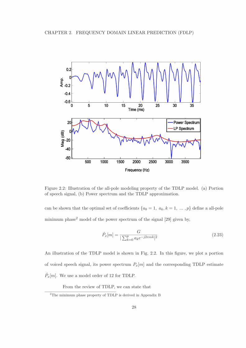
Figure 2.2: Illustration of the all-pole modeling property of the TDLP model. (a) Portionof speech signal, (b) Power spectrum and the TDLP approximation.
can be shown that the optimal set of coefficients a0 = 1, ak, k = 1, ... , p define a all-pole
minimum phase2 model of the power spectrum of the signal [29] given by,
Px[m] =G
|∑pk=0 ake
−j2πmk|2 (2.23)
An illustration of the TDLP model is shown in Fig. 2.2. In this figure, we plot a portion
of voiced speech signal, its power spectrum Px[m] and the corresponding TDLP estimate
Px[m]. We use a model order of 12 for TDLP.
From the review of TDLP, we can state that
2The minimum phase property of TDLP is derived in Appendix B
28
CHAPTER 2. FREQUENCY DOMAIN LINEAR PREDICTION (FDLP)
Proposition 1. The application of linear prediction in one domain will result in all-pole
minimum phase approximation of the squared magnitude of the dual domain
In the case of TDLP using time-domain auto-correlations (Eq. 2.14), Prop. 1 means
that LP model obtained by solving (Eq. 2.19) approximates the power spectrum (Eq: 2.17).
This proposition can be extended to modeling of temporal envelopes. For modeling the
Hilbert envelope of the signal, we need to apply linear prediction in its dual domain. In the
next section, we show that the dual of the Hilbert envelope is the auto-correlation of the
DCT sequence. Therefore, this implies that the application of linear prediction on
the DCT of a signal results in the AR model of the Hilbert envelope.
2.5 Frequency Domain Linear Prediction (FDLP)
Linear prediction in the spectral domain was first proposed by Kumaresan [26]. The analog
signal theory is used for developing the concept and the extension of the solution for a
discrete-sample case is provided. This was reformulated by Athineos [27, 34] using matrix
notations and the connection with DCT sequence is established. In our case, we derive the
discrete-time relations underlying the FDLP model without using matrix notations3. This
method mainly uses Fourier transform relations and AS spectrum definition. The proposed
derivation is simplistic and uses a mild assumption on the input signal.
In this section, we show the fundamental relation which relates the auto-correlation
of the DCT of the signal and the Hilbert envelope and use some of the properties of TDLP
stated in Sec. 2.4 to develop the FDLP model. The section ends with a comparison of the
3This derivation is identical to the matrix notation based derivation given in [27]. The arguments havebeen reformulated here to be more simplistic.
29
CHAPTER 2. FREQUENCY DOMAIN LINEAR PREDICTION (FDLP)
TDLP and FDLP techniques.
2.5.1 Discrete-Time Analytic Signal
The continuous time analytic signal (AS) defined by Gabor [12] has the property
that the spectrum of the AS is non-zero only for positive frequencies. However, for a
discrete-time signal, the DTFT spectrum is periodic with period of 2π and therefore cannot
be completely causal in the spectral domain. Thus, there is a need to define properties of
“analytic” like discrete signals.
The two-main properties of the continuous time AS (other than causal spectral
property) are that the real part of the AS corresponds to the observed signal and the real
and imaginary parts of the AS are orthogonal to each other. In a discrete-time case, a
“analytic” signal can be defined which satisfies these two properties [35]. The procedure for
defining the AS xa[n] of a discrete sequence x[n] are -
1. Compute the N-point DFT sequence X[k]
2. Find the N-point DFT of the AS as,
Xa[k] =
X[0] for k = 0
2X[k] for 1 ≤ k ≤ N2 − 1
X[N2 ] for k = N2
0 for N2 + 1 ≤ k ≤ N
(2.24)
3. Compute the inverse DFT of Xa[k] to obtain xa[n]
30

CHAPTER 2. FREQUENCY DOMAIN LINEAR PREDICTION (FDLP)
It can be shown that the above definition of discrete-time AS satisfies the required proper-
ties,
Re
xa[n]
= x[n] (2.25)
N−1∑
n=0
Re
xa[n]
Im
xa[n]
= 0 (2.26)
2.5.2 Relation between Auto-correlations of DCT and Hilbert Envelope
We assume that the discrete-time sequence x[n] has a zero-mean property in time and
frequency domains, i.e., x[0] = 0 and X[0] = 0. This assumption is made so as to give
a direct correspondence between the DCT of the signal and DFT [27]. Further, these
assumptions are mild and can be easily achieved by appending a zero in the time-domain
and removing the mean of the signal. Some of the relations shown here are a re-formulation
of the previous work done in [27].
The type-I odd DCT y[k] of a signal for k = 0, ... , N − 1 is defined as [31]
y[k] = 4
N−1∑
n=0
cn,kx[n] cos(2πnk
M
)
(2.27)
where the constants cn,k = 1 for n, k > 0 and cn,k = 12 for n, k = 0 and cn,k = 1√
2for the
values of n, k, where only one of the index is 0. The DCT defined by Eq. 2.27 is a scaled
version of the original orthogonal DCT with a factor of 2√M .
We also define the even-symmetrized version q[n] of the input signal,
q[n] =
x[n] for n = 0 , .., N − 1
x[M − n] for n = N, ... ,M − 1
(2.28)
31
CHAPTER 2. FREQUENCY DOMAIN LINEAR PREDICTION (FDLP)
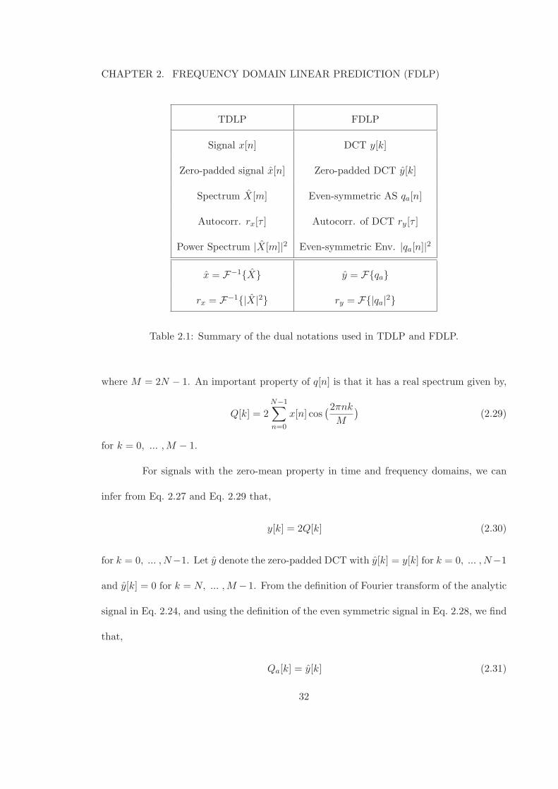
TDLP FDLP
Signal x[n] DCT y[k]
Zero-padded signal x[n] Zero-padded DCT y[k]
Spectrum X[m] Even-symmetric AS qa[n]
Autocorr. rx[τ ] Autocorr. of DCT ry[τ ]
Power Spectrum |X[m]|2 Even-symmetric Env. |qa[n]|2
x = F−1X y = Fqa
rx = F−1|X|2 ry = F|qa|2
Table 2.1: Summary of the dual notations used in TDLP and FDLP.
where M = 2N − 1. An important property of q[n] is that it has a real spectrum given by,
Q[k] = 2N−1∑
n=0
x[n] cos(2πnk
M
)
(2.29)
for k = 0, ... ,M − 1.
For signals with the zero-mean property in time and frequency domains, we can
infer from Eq. 2.27 and Eq. 2.29 that,
y[k] = 2Q[k] (2.30)
for k = 0, ... , N−1. Let y denote the zero-padded DCT with y[k] = y[k] for k = 0, ... , N−1
and y[k] = 0 for k = N, ... ,M −1. From the definition of Fourier transform of the analytic
signal in Eq. 2.24, and using the definition of the even symmetric signal in Eq. 2.28, we find
that,
Qa[k] = y[k] (2.31)
32
CHAPTER 2. FREQUENCY DOMAIN LINEAR PREDICTION (FDLP)
for k = 0, ... ,M −1. This says that the AS spectrum of the even-symmetric signal is equal
to the zero-padded DCT signal. In other words, the inverse DFT of the zero-padded DCT
signal is the even-symmetric AS. This is similar to the relation between the zero-padded
signal x[n] (defined in Eq. 2.15) and its Fourier transform X[m] defined in Eq. 2.16. Since
the auto-correlation of signal x[n] is related to the power spectrum |X[m]|2 (Eq. 2.17), we
can obtain a similar relation to the auto-correlation of the DCT sequence. In order to clarify
the analysis, we have illustrated the various duality relation in Table. 2.1.
The auto-correlation of the DCT signal is defined as (similar to Eq. 2.14),
ry[τ ] =1
N
N−1∑
k=|τ |y[k]y[k − |τ |] (2.32)
From Eq. 2.31, the inverse DFT of zero-padded DCT signal y[k] is the AS of the even-
symmetric signal (similar to Eq. 2.16). Analogous to Eq. 2.17, it can be shown that,
ry[τ ] =1
N
M−1∑
n=0
|qa[n]|2e−j 2πnτM (2.33)
i.e., the auto-correlation of the DCT signal and the squared magnitude of the AS (Hilbert
envelope) of the even-symmetric signal are Fourier transform pairs. This is exactly dual to
the relation in Eq. 2.17.
By invoking Prop. 1, we can deduce that
Proposition 2. Proposition Linear prediction of DCT components results in AR model of
the Hilbert envelope of the even-symmetrized signal.
In deriving this proof, one could relax the mild assumptions of zero-mean property
in time and frequency domains and prove the above result for a general signal. But, this
would mean the modification of the definition of the DCT to account for the scaling of
33
CHAPTER 2. FREQUENCY DOMAIN LINEAR PREDICTION (FDLP)
the first DCT index [27]. Once the set of FDLP coefficients ak are estimated by linear
prediction on DCT, the resulting FDLP envelope is given by,
Ex(n) =G
|∑k=pk=0 ake
−i2πkn|2(2.34)
It is important to note that the above analysis is valid only for the type-I odd DCT
(Eq. 2.27) which is directly related to the DFT. Although, AR modeling on other types of
DCT has been studied in the past [38], we limit the scope of this thesis to the type-I odd
DCT. In the next section, we show the illustration of the FDLP model for speech examples.
2.5.3 Examples
FDLP versus TDLP
The comparison the TDLP and FDLP is shown in Fig. 2.3. Here we plot (a)
a portion of a speech signal, (b) the power spectrum and its approximation by TDLP
model and (c) the Hilbert envelope computed using the DFT technique (Eq. 2.24) and the
FDLP envelope. Both these AR modeling techniques approximate the peak regions more
accurately than the valleys. This is useful in speech applications as the high-energy regions
are perceptually more important. Later in the thesis, we show that this property is also
useful in robust representation in the noisy and reverberant environments.
FDLP Modeling of Full-Band Speech
Unlike some of the other methods of demodulation discussed in Sec. 1.2.1, the
FDLP method can be used to summarize the energy variations of long temporal regions
34
CHAPTER 2. FREQUENCY DOMAIN LINEAR PREDICTION (FDLP)
0 500 1000 1500 2000 2500 3000 3500 4000
40
60
80
100
Frequency (Hz)
Mag
. (dB
)
(b)
5 10 15 20 25 30 35
−2000
0
2000
Time (ms)
Am
p.
(a)
5 10 15 20 25 30 35
40
60
Time (ms)
Mag
. (dB
)
(c)
Hilbert Envelope
FDLP Envelope
Power Spectrum
LP Spectrum
Figure 2.3: (a) A portion of speech signal, (b) Spectral AR model (TDLP) and (c) TemporalAR model (FDLP).
of wide-band speech signals. We demonstrate this property in Fig. 2.4. where we plot a
portion of speech signal, its Hilbert envelope computed from the analytic signal [35] and the
AR model fit to the Hilbert envelope using FDLP. The peaks in the FDLP model correspond
to pole locations and the number of peaks is at most equal to half the model order used in
FDLP. In this figure, we use a model order of 40 on the full-band signal of duration 500 ms.
AM-FM Decomposition Using FDLP
For many modulated signals in the real world, the quadrature version of a real
input signal and its Hilbert transform are identical [14, 15]. This means that the Hilbert
envelope is the squared AM envelope of the signal and the operation of FDLP estimates the
35
CHAPTER 2. FREQUENCY DOMAIN LINEAR PREDICTION (FDLP)
0 50 100 150 200 250 300 350 400 450 500 550−2
0
2x 10
4 (a)
0 50 100 150 200 250 300 350 400 450 500 5500
1
2
3
4x 10
8 (b)
0 50 100 150 200 250 300 350 400 450 500 5500
1
2
3
4x 10
8
Time (ms)
(c)
Figure 2.4: Illustration of the AR modeling property of FDLP. (a) a portion of speechsignal, (b) its Hilbert envelope and (c) all pole model obtained using FDLP.
AM envelope of the signal and the FDLP residual contains the FM component of the signal.
AM-FM decomposition using FDLP technique consists of two steps. In the first step, the
envelope of the signal is approximated with an AR model by using the linear prediction in
the DCT domain. The resulting residual signal is obtained by dividing the original signal
with the AR model of the Hilbert envelope obtained in the first step [26]. This forms a
parametric approach to AM-FM decomposition of a signal. FM components are used in
audio coding applications (Chap. 6).
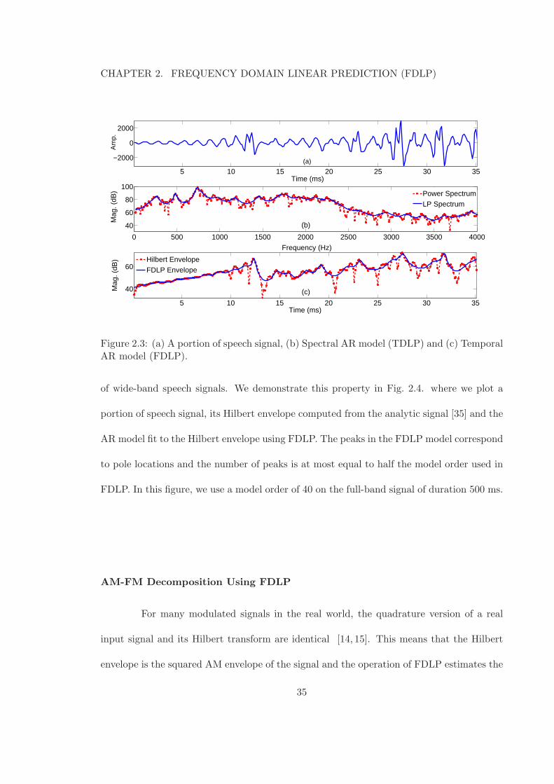
Speech signals in sub-bands are modulated signals [18] and hence, FDLP technique
can be used for AM-FM decomposition of sub-band signals. An illustration of the AM-
36
CHAPTER 2. FREQUENCY DOMAIN LINEAR PREDICTION (FDLP)
0 100 200 300 400 500 600 700−5000
0
5000A
mpl
itude
(a)
0 100 200 300 400 500 600 7000
2000
4000
Am
plitu
de
(b)
0 100 200 300 400 500 600 700−2
0
2
Time (ms)
Am
plitu
de
(c)
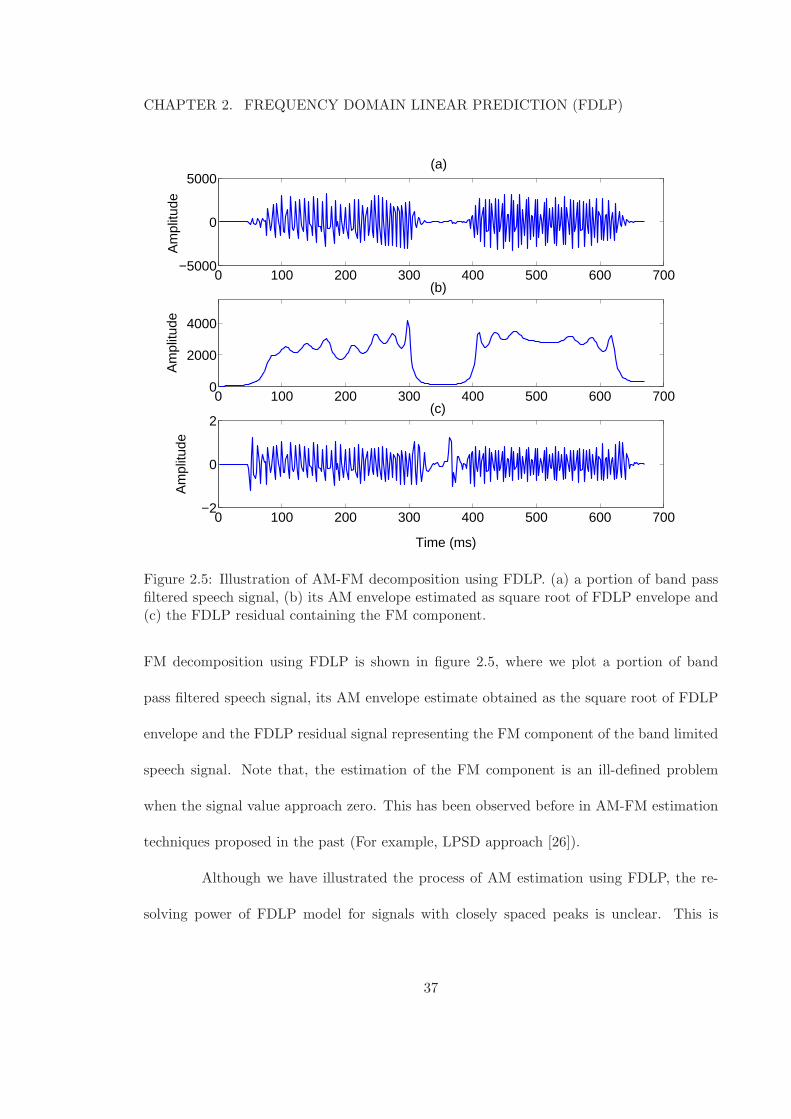
Figure 2.5: Illustration of AM-FM decomposition using FDLP. (a) a portion of band passfiltered speech signal, (b) its AM envelope estimated as square root of FDLP envelope and(c) the FDLP residual containing the FM component.
FM decomposition using FDLP is shown in figure 2.5, where we plot a portion of band
pass filtered speech signal, its AM envelope estimate obtained as the square root of FDLP
envelope and the FDLP residual signal representing the FM component of the band limited
speech signal. Note that, the estimation of the FM component is an ill-defined problem
when the signal value approach zero. This has been observed before in AM-FM estimation
techniques proposed in the past (For example, LPSD approach [26]).
Although we have illustrated the process of AM estimation using FDLP, the re-
solving power of FDLP model for signals with closely spaced peaks is unclear. This is
37

CHAPTER 2. FREQUENCY DOMAIN LINEAR PREDICTION (FDLP)
0 20 40 60 80 100 1200
0.2
0.4
0.6
0.8
1
Am
p
(a)
0 20 40 60 80 100 120−40
−20
0
Log
Env
, (dB
)
Time (ms)
(b)
0 20 40 60 80 100 1200
0.2
0.4
0.6
0.8
1
Am
p.
(c)
0 20 40 60 80 100 120−40
−20
0(d)
Time (ms)
Log
Env
. (dB
)
Figure 2.6: Plot of 125 ms of input signal in time domain (a), (c) and the correspondinglog FDLP envelopes (b), (d).
important as the result of the resolution analysis may provide insight to the selection of
the model-order as well as the choice of DCT window type. These studies can be analo-
gously extended to determine the spectral resolution of a TDLP model. To the best of our
knowledge, these studies have not been done in the past for TDLP.
2.6 Temporal Resolution Analysis in FDLP
In this section, we analyze the temporal resolution in FDLP models using signals
with distinct temporal peaks (impulses). We use artificial signals for this analysis and
compute FDLP models on the full-band DCT signal (as opposed to sub-band FDLP models
used in speech feature extraction discussed in Chap. 4). The main factors considered here
38
CHAPTER 2. FREQUENCY DOMAIN LINEAR PREDICTION (FDLP)
are the type of the DCT window, relative position of the temporal peak within the analysis
window, model order for FDLP and type of LP method used (auto-correlation LP versus
least squares LP). Before we discuss the resolution properties of FDLP, we propose an
objective method to determine temporal resolution.
2.6.1 Defining the Temporal Resolution
We generate a signal with two peaks as shown in Fig. 2.6(a). The FDLP envelope
of this signal (Fig. 2.6(c)) is computed by the application of linear prediction on DCT com-
ponents. As seen in Fig. 2.6(a),(c), if the input signal has peaks which are far enough, two
distinct peaks emerge in the FDLP envelope. As the spacing between the input peaks is de-
creased (Fig. 2.6(b)), the resulting peaks in the FDLP envelope start merging (Fig. 2.6(d)).
The time interval between the two peaks in the input signal below which the resulting peaks
in the FDLP envelope merge to form a single peak is referred to as the critical time-span.
We define the resolution as the inverse of the critical time-span. We obtain the normalized
resolution by dividing the resolution with the maximum possible resolution - the inverse of
the minimum duration between the input signal peaks. In order to determine the resolution
of the FDLP model, we use a peak picking mechanism on the log FDLP envelope.
In the discussions that follow, the input signal has two distinct peaks and the
interval between the two peaks is varied. The FDLP envelope for this signal is input to the
peak picking algorithm and the critical time-span is used to calculate the resolution.
39
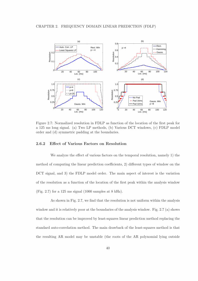
CHAPTER 2. FREQUENCY DOMAIN LINEAR PREDICTION (FDLP)
20 40 60 80 100 1200
0.2
0.4
0.6
0.8
Loc. (ms)
Res
olut
ion
(b)
20 40 60 80 100 1200
0.25
0.5
0.75
1.0
(c)
Loc. (ms)
Res
olut
ion
p=4
p=8
p=16
0 20 40 60 80 100 1200
0.25
0.5
0.75
1.0
(d)
Loc. (ms)R
esol
utio
n
No Pad
Pad 16ms
Pad 32ms
20 40 60 80 1000
0.1
0.2
(a)
Loc. (ms)
Res
olut
ion
Auto. Corr. LP
Least Squares LP
Rect.
Hamming
Gauss.
Rect. Winp = 4
Gauss. Winp =8Gauss. Win
p =4
Figure 2.7: Normalized resolution in FDLP as function of the location of the first peak fora 125 ms long signal. (a) Two LP methods, (b) Various DCT windows, (c) FDLP modelorder and (d) symmetric padding at the boundaries.
2.6.2 Effect of Various Factors on Resolution
We analyze the effect of various factors on the temporal resolution, namely 1) the
method of computing the linear prediction coefficients, 2) different types of window on the
DCT signal, and 3) the FDLP model order. The main aspect of interest is the variation
of the resolution as a function of the location of the first peak within the analysis window
(Fig. 2.7) for a 125 ms signal (1000 samples at 8 kHz).
As shown in Fig. 2.7, we find that the resolution is not uniform within the analysis
window and it is relatively poor at the boundaries of the analysis window. Fig. 2.7 (a) shows
that the resolution can be improved by least-squares linear prediction method replacing the
standard auto-correlation method. The main drawback of the least-squares method is that
the resulting AR model may be unstable (the roots of the AR polynomial lying outside
40
CHAPTER 2. FREQUENCY DOMAIN LINEAR PREDICTION (FDLP)
the unit-circle). However, as observed in TDLP studies [29], this can be partially alleviated
when the number of samples N is significantly larger than model order p. Fig. 2.7 (b) shows
that the Gaussian window in the DCT domain provides good temporal resolution among
various window types considered here4. An increase in the model order also improves the
resolution as shown in Fig. 2.7 (c). However, a significant increase in the model order may
result in the modeling of finer temporal details in the signal which are more vulnerable to
noise.
In Fig. 2.7 (d), we provide one possible solution for improving the resolution at the
boundaries of the analysis window. This is done by symmetric padding of the signal at the
beginning and end of the analysis window. Once the FDLP envelope is derived, the portion
of the envelope in the padded regions can be ignored. This eliminates the lower resolution
parts of the FDLP model and improves the temporal resolution within the region of interest.
We find that about 32 ms of padding provides good resolution at the boundaries.
In order to illustrate the effect of improved resolution in clean and noisy speech signals,
the FDLP envelopes are estimated from sub-band (700-1100Hz) DCT components for clean
speech and noisy speech (babble noise at 10 dB). Fig. 2.8 (a) and (b) shows the plot of the
envelopes without and with the modifications developed for higher resolution. As seen in
this figure, estimating high resolution envelopes from noisy speech reduces the mismatch
between clean and noisy conditions without making any assumptions about the noise.
4In other experiments, Hanning window also provided high resolution as there are no discontinuities atthe edges. The effect of window type on the final resolution is not completely understood and further analysismay be required.
41

CHAPTER 2. FREQUENCY DOMAIN LINEAR PREDICTION (FDLP)
100 200 300 400 500 600 700
0
20
40
Log
Env
. (dB
)
(a)
100 200 300 400 500 600 700
40
60
80
Time (ms)
Log
Env
. (dB
)
(b)
CleanBabble
CleanBabble
Figure 2.8: Log FDLP envelopes from clean and noisy (babble at 10 dB) sub-band speech.(a) Low resolution envelopes and (b) High resolution envelopes.
2.7 Chapter Summary
In this chapter, we have described various methods for AR modeling of Hilbert
envelopes. An outline of the important results in deriving the conventional TDLP was
given. Then, a detailed derivation of the underlying model of FDLP was provided. The
properties of FDLP for AM-FM decomposition were illustrated with a few examples and
the effect of various parameters on the temporal resolution of FDLP was also investigated.
In the succeeding chapters, we extend the FDLP model for various speech and
audio applications. A number of other parameters in the FDLP model, like the duration
of the temporal analysis window, the type of sub-band decomposition, DCT window shape
and importance of the gain parameter G will also be investigated. An optimal choice of
these parameters is chosen for recognition experiments based on the performance in clean
42
CHAPTER 2. FREQUENCY DOMAIN LINEAR PREDICTION (FDLP)
and noisy conditions (discussed in Chap. 4).
In the next chapter, we focus the effect of reverberation on the gain parameter
and provide a solution for robust representation in the presence of these artifacts.
43
Chapter 3
Gain Normalization of FDLP
Envelopes
3.1 Chapter Outline
Reverberation continues to be a challenging problem for speech recognition sys-
tems as it causes mis-match in training and test conditions. This results in a significant
degradation in performance. In this chapter, we try to address this issue by developing the
gain normalization technique for FDLP which attempts to create a robust representation
in the reverberant environments.
We begin the chapter with a discussion of the problem of reverberation as a long-
term convolutive artifact (Sec. 3.2). Some of the methods proposed in the past to deal
with reverberation artifacts in speech recognition are reviewed next (Sec. 3.3). The effect of
reverberation on sub-band Hilbert envelopes is analyzed in Sec. 3.4. Then, we propose the
44
CHAPTER 3. GAIN NORMALIZATION OF FDLP ENVELOPES
gain normalization technique which attempts to suppress reverberation artifacts (Sec. 3.5.
This is illustrated using a few examples of reverberant speech signals (Sec. 3.6). The chap-
ter ends with a discussion on the application of gain normalization for speech recognition
(Sec. 3.7).
This chapter does not discuss the speech recognition experiments using the gain
normalization technique. These results are described in Chap. 4
3.2 Room Reverberation
When speech is recorded in far-field reverberant environments, the data collected in
the microphone consist of the direct speech component superimposed with multiple number
of reflections. These reflections present themselves as delayed and attenuated versions of
the original signal. The superposition can be modeled as a convolution of the clean speech
signal with the room response function, i.e.,
r(t) = x(t) ∗ h(t), (3.1)
where s(t), h(t) and r(t) denote the original speech signal, the room impulse response and
the reverberant speech respectively. If we apply a long-term Fourier transform, we can
write,
R(k) = X(k)×H(k). (3.2)
For Eq. 3.2 to be valid, the Fourier transforms R(ω), X(ω) and H(ω) have to computed
using segments which are longer than the duration of h(t). However, a room response is
generally not time-limited. The amount of reverberation in speech is generally characterized
45
CHAPTER 3. GAIN NORMALIZATION OF FDLP ENVELOPES
by reverberation time (T60). T60 denotes the amount of time required for the reverberant
signal to reduce by 60 dB from the initial direct component value. The value of T60 ranges
from 200ms-800ms for typical meeting room scenarios. Human speech perception can toler-
ate moderate levels of reverberation. For highly reverberant environments (with high values
of T60), the speech intelligibility reduces [20].
The effect of reverberation on the short-time Fourier transform (STFT) (defined
in Eq. 1.3) can be represented as a convolution,
R(t, ω) = X(t, ω) ∗[
h(t)ejωt]
, (3.3)
where S(t, ωk) and R(t, ωk) are the STFT’s of the clean speech signal s(t) and reverberant
speech r(t) respectively. Thus, convolution of the signal in the time-domain (Eq. 3.1) would
result in a convolution of the STFT for each frequency component with the room impulse
response. In the case of room reverberation h(t) with large T60 values and for STFT window
length which is smaller than the T60, the STFT of clean speech, X(t, ω), cannot be easily
recovered from R(t, ω). For speech recognition models which are trained using STFT’s of
clean speech, this would create a high degree of mis-match.
In the next section, we review some of the approaches proposed in the past to deal
with the mis-match caused by convolutions. Some of these approaches are based on STFT
for removing short-term distortions. However, they do not entirely suppress the long-term
artifacts like room-reverberation.
46
CHAPTER 3. GAIN NORMALIZATION OF FDLP ENVELOPES
3.3 Past Approaches For Suppressing Convolutive Artifacts
3.3.1 Cepstral Mean Subtraction (CMS)
Cepstral mean subtraction is the technique of removing linear distortions and
short-term convolutive artifacts by removing the mean of the cepstral sequence [39]. When
speech signal is convolved with a linear channel (similar to Eq. 3.1) with the duration of
the response smaller than the STFT analysis window, the STFT of the convolved output
can be written as,
R(t, ω) ≃ H(ω)X(t, ω) (3.4)
For feature extraction in speech, the STFT magnitudes are typically warped to a non-
linear frequency scale by a weighted summation. Log-DCT is applied to obtain the cepstral
sequence. In the cepstral domain, this distortion will appear as an offset term, i.e., every
cepstral frame will have a frame-independent additional term from the channel [39]. Thus,
removing the mean of the cepstral sequence computed over the utterance (assuming the
channel is stationary) can remove this convolutive artifact.
However, the fundamental assumption in Eq. 3.4 is the short-term nature of re-
sponse function h(t). For reverberation artifacts, the typical response function is much
longer in duration compared to the STFT window (w(t)) length. If the response function
h(t) is assumed to be the sum of early reflections hl(t) (which last only up to the dura-
tion of w(t)) and late reflections he(t) (which represents the remaining part of the response
function h(t)), then the CMS technique can suppress the early reflection part. The late
reflections are not removed in the CMS approach.
47

CHAPTER 3. GAIN NORMALIZATION OF FDLP ENVELOPES
3.3.2 Log-DFT Mean Normalization (LDMN)
In CMS, there is an underlying assumption that the channel response is constant
in each critical band. However, the typical response functions do not have a constant value
in each critical band and thus, the mean subtraction should be done in a linear frequency
scale [40] (as opposed to the mean subtraction in a warped frequency scale done in CMS).
Log-DFT mean normalization technique (LDMN) tries to remove channel distor-
tions by removing mean of the log STFT magnitude in a linear frequency scale [40]. For
speech recognition experiments the LDMN approach performs better than the CMS tech-
nique as the assumptions on the channel response are less stringent. However, the LDMN
approach also suffers from the late reflections as this approach (similar to the CMS) can
effectively suppress only the early reflection part.
3.3.3 Long-term Log Spectral Subtraction (LTLSS)
In order to make the mean subtraction effective in reverberant conditions, it is
necessary to estimate the log-spectrum from long-term windows. This would mean that
the window length is longer than the T60 of the room response function. By deriving long-
term spectrum of speech, the room response function will be multiplicative in the spectral
domain (similar to Eq. 3.4) and additive in the log-spectral domain. The mean of long-
term log-spectrum computed from a sequence of windowed speech segments can be used
as an estimate of the log-spectrum of the room response function. A mean subtraction in
log-spectral domain can achieve the desired robustness.
This approach was used in [41] to suppress the reverberation artifacts of speech
48
CHAPTER 3. GAIN NORMALIZATION OF FDLP ENVELOPES
signal. The method involves the subtraction of a mean estimate of the log spectrum using a
long-term (2s) analysis window, followed by overlap-add re-synthesis to obtain the enhanced
speech. The processed signal is used for speech recognition in reverberant environments
where the LTLSS method provides good improvements.
The underlying assumption in LTLSS is that the room-response is stationary over
the window of the mean computation. Since the mean is computed on set of long-term log-
spectral frames, the window of mean computation is substantially long (of the order of 30s
obtained by concatenating all speech files from the same speaker [41]). Thus, the technique
requires the recording of long-segments of speech from the same speaker and environment.
However, the approach is effective for scenarios where such long-segments are available.
3.4 Envelope Convolution Model
In Chap. 2, we had developed the FDLP technique as an AM-FM model for the
analysis of speech signal in sub-bands. In particular, the FDLP model estimates the AM
component of the signal (Sec. 2.5). Since the AR model estimates the peaks with high
accuracy, these estimates are relatively well preserved in noisy conditions. Thus, we can in-
tuitively claim that FDLP based approaches should provide robust representation of speech
signals. If the FDLP model is applied for processing a speech signal in reverberant envi-
ronments, the resulting AM envelopes are modified. In this section, we analyze the effect
of the room-reverberation on these envelopes.
Specifically, we show the relation between AM component of the reverberant signal
and the AM component of clean speech. For narrow band signals analyzed in long-temporal
49
CHAPTER 3. GAIN NORMALIZATION OF FDLP ENVELOPES
windows, it can be shown that the envelope of reverberant signal is equal to the convolution
of the clean speech envelope and room response envelope except for a scaling factor [42].
Let xq(t), hq(t) and rq(t) denote the sub-band clean speech, room-response and
the reverberant speech respectively and q = 1, ... , Q denote the sub-band index. Assuming
an ideal band-pass filtering we can write (using Eq. 3.1),
rq(t) = xq(t) ∗ hq(t). (3.5)
Now, the analytic signal raq(t) = rq(t) +H[rq(t)] can be shown to be (Appendix A.3),
raq(t) =1
2xaq(t) ∗ haq(t), (3.6)
Using the polar form of the analytic signal (Eq. 2.4), we can write,
mr(t)ejφr(t) =
1
2
∫ ∞
−∞mx(t− τ)ejφx(t−τ)mh(τ)e
jφh(τ)dτ (3.7)
wheremr(t), mx(t), mh(t) denote the sub-band AM component of reverberant speech, clean
speech and room response respectively and φr(t), φx(t), φh(t) denote the sub-band phase
modulation component of reverberant speech, clean speech and room response1.
For a narrow-band analysis (Q >> 1) on long-term segments, we can approximate
the phase modulation components of clean speech and room response as [42],
φx(t) = ω0t+Φq(t), (3.8)
φh(t) = ω0t (3.9)
where ω0 denotes the center frequency of the narrow band q. Further, if phase modulation
Φq(t) in speech is assumed to be slowly varying compared to the envelope, we can write
1Note that, we have dropped the sub-band index sub-script on the modulation components forconvenience.
50
CHAPTER 3. GAIN NORMALIZATION OF FDLP ENVELOPES
Eq. 3.7 as,
mr(t)ejφr(t) ≃ 1
2ej(ω0t+Φq(t))
∫ ∞
−∞mx(t− τ)mh(τ)dτ (3.10)
Applying magnitude on both sides, we get the relation between AM components of the
reverberant signal and the clean speech signal.
mr(t) ≃1
2mx(t) ∗mh(t), (3.11)
In other words, for each narrow-band, the modulation spectrum of reverberant speech2,
Mr(ω)F⇐⇒ mr(t), is equal to half the product of modulation spectrum of clean
speech Mx(ω) with that of the room-response function Mh(ω).
In the next section, we use this relation to suppress the effects of reverberation
artifacts in speech signals.
3.5 Robust Envelope Estimation With Gain Normalization
In this section, we extend the analysis of Sec. 3.4 to develop the gain normaliza-
tion technique [43]. In order to develop this extension, we use an assumption about the
characteristics of typical room-response functions. When speech is analyzed over long-term
windows in narrow sub-bands (band-width less than 100 Hz), the modulation spectrum of
the room-response function can be assumed to be flat compared to the modulation spectrum
of clean speech signal. For example, the sub-band (750− 850 Hz) modulation spectrum of
clean speech3 envelope (Mx(ω)) is shown in Fig. 3.1(a). Similarly, the sub-band modulation
2The definition of the modulation spectrum used here is different from the modulation spectrum usedin Chap. 5. In Chap. 5, we obtain the modulation spectrum as the Fourier transform of the compressedenvelope. For defining the modulation spectrum here, we do not apply any compression.
3We use the clean speech data from TIDIGTS database - “FAK 86Z1162A.wav”
51
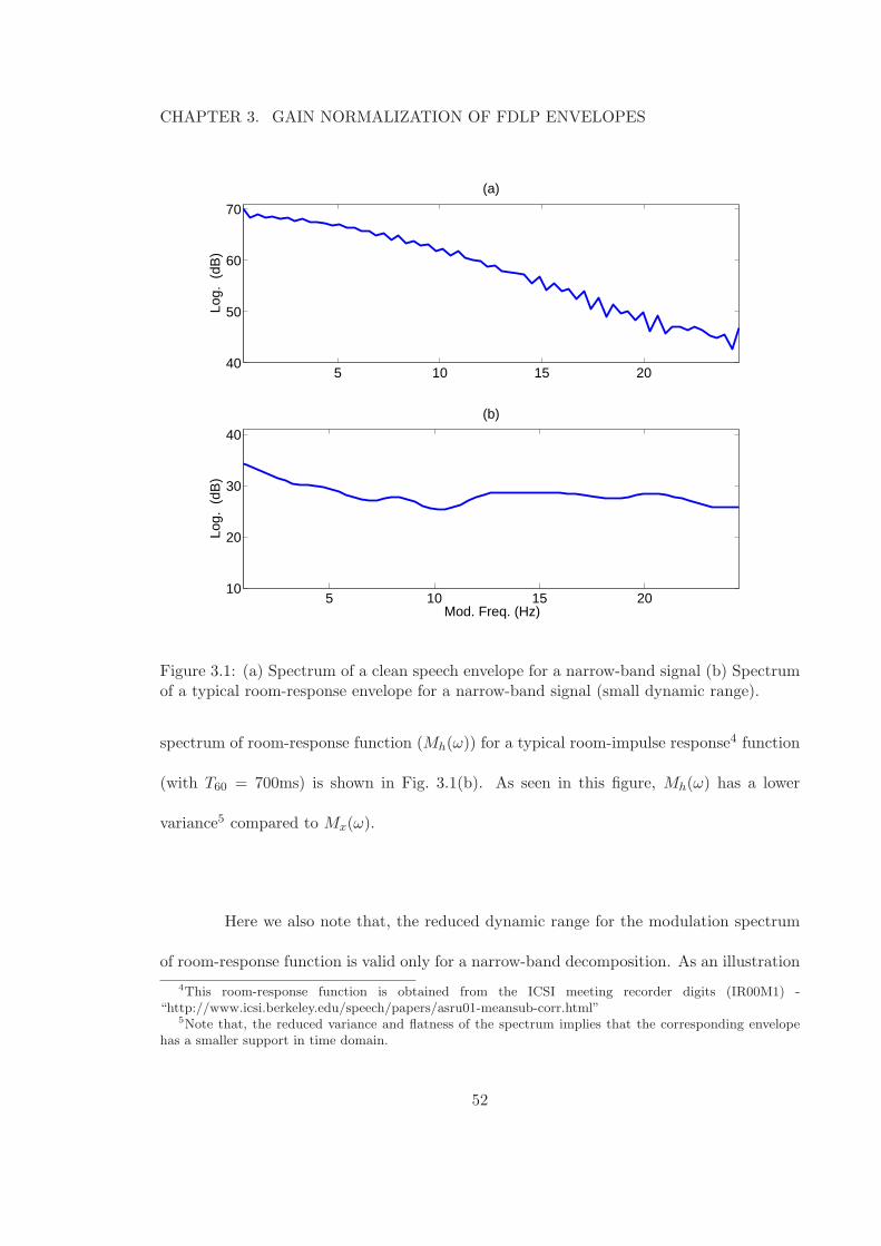
CHAPTER 3. GAIN NORMALIZATION OF FDLP ENVELOPES
5 10 15 2040
50
60
70Lo
g. (
dB)
(a)
5 10 15 2010
20
30
40
Mod. Freq. (Hz)
Log.
(dB
)
(b)
Figure 3.1: (a) Spectrum of a clean speech envelope for a narrow-band signal (b) Spectrumof a typical room-response envelope for a narrow-band signal (small dynamic range).
spectrum of room-response function (Mh(ω)) for a typical room-impulse response4 function
(with T60 = 700ms) is shown in Fig. 3.1(b). As seen in this figure, Mh(ω) has a lower
variance5 compared to Mx(ω).
Here we also note that, the reduced dynamic range for the modulation spectrum
of room-response function is valid only for a narrow-band decomposition. As an illustration
4This room-response function is obtained from the ICSI meeting recorder digits (IR00M1) -“http://www.icsi.berkeley.edu/speech/papers/asru01-meansub-corr.html”
5Note that, the reduced variance and flatness of the spectrum implies that the corresponding envelopehas a smaller support in time domain.
52
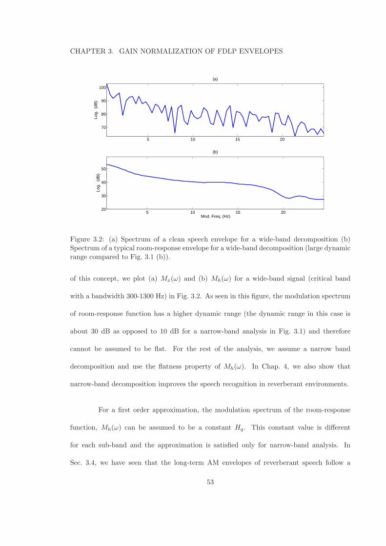
CHAPTER 3. GAIN NORMALIZATION OF FDLP ENVELOPES
5 10 15 2020
30
40
50
Mod. Freq. (Hz)
Log.
(dB
)
(b)
5 10 15 20
70
80
90
100
Log.
(dB
)
(a)
Figure 3.2: (a) Spectrum of a clean speech envelope for a wide-band decomposition (b)Spectrum of a typical room-response envelope for a wide-band decomposition (large dynamicrange compared to Fig. 3.1 (b)).
of this concept, we plot (a) Mx(ω) and (b) Mh(ω) for a wide-band signal (critical band
with a bandwidth 300-1300 Hz) in Fig. 3.2. As seen in this figure, the modulation spectrum
of room-response function has a higher dynamic range (the dynamic range in this case is
about 30 dB as opposed to 10 dB for a narrow-band analysis in Fig. 3.1) and therefore
cannot be assumed to be flat. For the rest of the analysis, we assume a narrow band
decomposition and use the flatness property of Mh(ω). In Chap. 4, we also show that
narrow-band decomposition improves the speech recognition in reverberant environments.
For a first order approximation, the modulation spectrum of the room-response
function, Mh(ω) can be assumed to be a constant Hq. This constant value is different
for each sub-band and the approximation is satisfied only for narrow-band analysis. In
Sec. 3.4, we have seen that the long-term AM envelopes of reverberant speech follow a
53
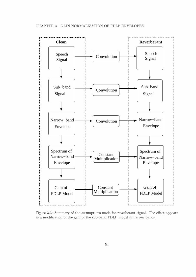
CHAPTER 3. GAIN NORMALIZATION OF FDLP ENVELOPES
Signal
Sub−band
Convolution
Convolution
ConvolutionNarrow−band
Envelope
Signal
Sub−band
Envelope
Narrow−band
Envelope
Spectrum ofNarrow−band Constant
Multiplication
FDLP Model
Gain of
Envelope
Spectrum of
Narrow−band
FDLP Model
Gain ofConstantMultiplication
SpeechSignal
SpeechSignal
ReverberantClean
Figure 3.3: Summary of the assumptions made for reverberant signal. The effect appearsas a modification of the gain of the sub-band FDLP model in narrow bands.
54
CHAPTER 3. GAIN NORMALIZATION OF FDLP ENVELOPES
convolution model (Eq. 3.11). When Mh(ω) is a constant, the envelope of reverberant
speech is approximated as mr(t) ≃ Hq
2 mx(t).
In the FDLP technique, this approximation would mean that auto-correlations
of each sub-band DCT signal (ry[τ ] defined in Eq. 2.33) would be scaled by an unknown
constantH2
q
4 . In a linear prediction framework, scaling the auto-correlations by a constant
would alter only the gain of the LP model G, and the predictor coefficients a1, a2, ..., ap
are unaltered.
Therefore, we arrive at the following proposition,
Proposition 3. The effect of room reverberation in narrow sub-bands can be suppressed by
setting the gain of the FDLP model to unity.
Using G = 1, the shape of the sub-band FDLP envelope is not modified. A scale
factor alone is removed over the entire trajectory. The gain normalized FDLP envelopes in
each band are derived (similar to Eq. 2.34) as,
Ex(n) =1
|∑k=pk=0 ake
−i2πkn|2(3.12)
It is important to note that the suppression of long-term artifacts like reverberation (using
gain normalization) also performs the suppression of short-term artifacts like linear channel
distortions (equivalent to CMS). This is possible because short-term response function can
fit well inside the analysis window and the envelope convolution model is satisfied.
We summarize the assumptions used in the suppression of the room-reverberation
in Fig. 3.3. The effect of reverberation at the signal and sub-band level is that of a con-
volution. For narrow-band analysis, we can represent this effect as the convolution of the
envelope of the sub-band signal. The modulation spectrum of the sub-band room-response
55
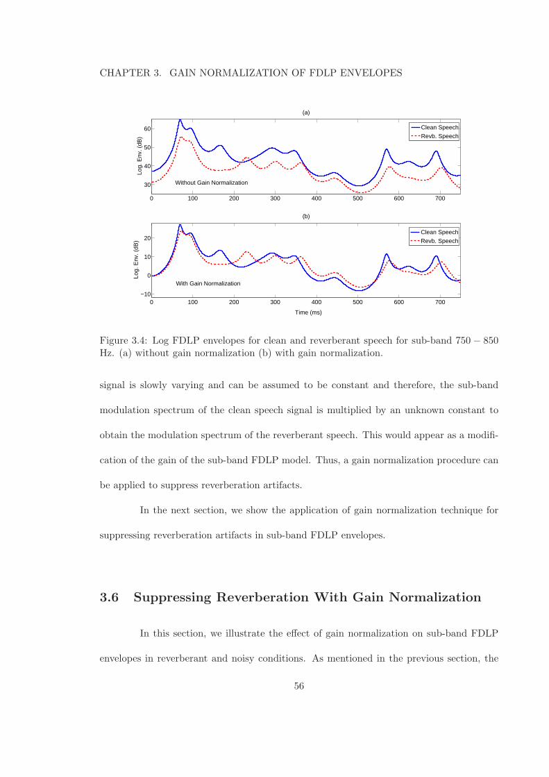
CHAPTER 3. GAIN NORMALIZATION OF FDLP ENVELOPES
0 100 200 300 400 500 600 700
30
40
50
60
Log.
Env
. (dB
)
(a)
0 100 200 300 400 500 600 700−10
0
10
20
Time (ms)
Log.
Env
. (dB
)
(b)
Clean Speech
Revb. Speech
Clean Speech
Revb. Speech
Without Gain Normalization
With Gain Normalization
Figure 3.4: Log FDLP envelopes for clean and reverberant speech for sub-band 750 − 850Hz. (a) without gain normalization (b) with gain normalization.
signal is slowly varying and can be assumed to be constant and therefore, the sub-band
modulation spectrum of the clean speech signal is multiplied by an unknown constant to
obtain the modulation spectrum of the reverberant speech. This would appear as a modifi-
cation of the gain of the sub-band FDLP model. Thus, a gain normalization procedure can
be applied to suppress reverberation artifacts.
In the next section, we show the application of gain normalization technique for
suppressing reverberation artifacts in sub-band FDLP envelopes.
3.6 Suppressing Reverberation With Gain Normalization
In this section, we illustrate the effect of gain normalization on sub-band FDLP
envelopes in reverberant and noisy conditions. As mentioned in the previous section, the
56
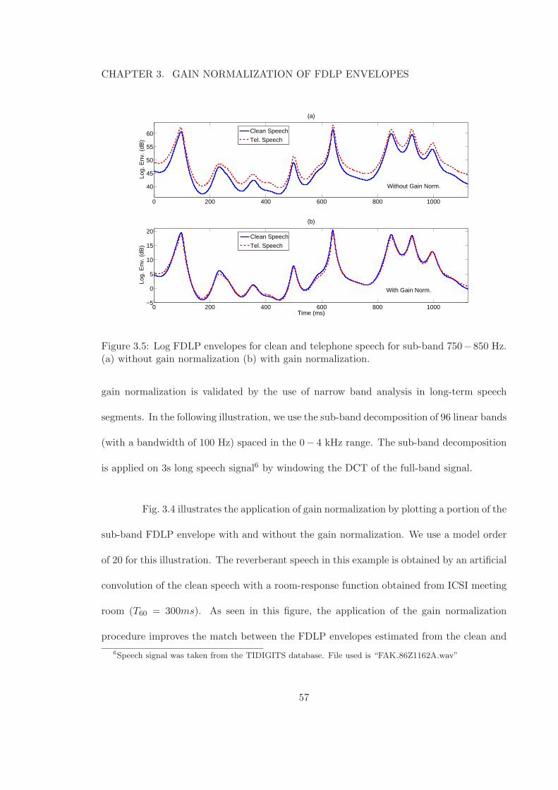
CHAPTER 3. GAIN NORMALIZATION OF FDLP ENVELOPES
0 200 400 600 800 1000
40
45
50
55
60Lo
g. E
nv. (
dB)
(a)
0 200 400 600 800 1000−5
0
5
10
15
20
Time (ms)
Log.
Env
. (dB
)
(b)
Clean Speech
Tel. Speech
Clean Speech
Tel. Speech
Without Gain Norm.
With Gain Norm.
Figure 3.5: Log FDLP envelopes for clean and telephone speech for sub-band 750−850 Hz.(a) without gain normalization (b) with gain normalization.
gain normalization is validated by the use of narrow band analysis in long-term speech
segments. In the following illustration, we use the sub-band decomposition of 96 linear bands
(with a bandwidth of 100 Hz) spaced in the 0− 4 kHz range. The sub-band decomposition
is applied on 3s long speech signal6 by windowing the DCT of the full-band signal.
Fig. 3.4 illustrates the application of gain normalization by plotting a portion of the
sub-band FDLP envelope with and without the gain normalization. We use a model order
of 20 for this illustration. The reverberant speech in this example is obtained by an artificial
convolution of the clean speech with a room-response function obtained from ICSI meeting
room (T60 = 300ms). As seen in this figure, the application of the gain normalization
procedure improves the match between the FDLP envelopes estimated from the clean and
6Speech signal was taken from the TIDIGITS database. File used is “FAK 86Z1162A.wav”
57
CHAPTER 3. GAIN NORMALIZATION OF FDLP ENVELOPES
reverberant speech. This match is relatively better in the high energy peaks of the speech
signal which are perceptually important. When features for speech recognition are derived
from FDLP envelopes, the application of gain normalization increases the invariance of the
features derived in clean and reverberant conditions. This would reflect in an improvement
in performance of these systems in mis-matched train/test conditions (Chap. 4).
As mentioned in Sec. 3.5, the gain normalization also improves the robustness
in short-term telephone distortions. This is illustrated in Fig. 3.5, where we plot the log
FDLP envelopes in clean and telephone channel conditions7. This plot is obtained for a
sub-band 750−850Hz of clean speech and the telephone speech. The telephone data is a re-
recording of the clean speech passed through a telephone channel. As shown in Fig. 3.5(b),
the envelopes extracted in telephone channel conditions match with those obtained from
the clean speech.
3.7 Chapter Summary
In this chapter, we have developed the gain normalization procedure for FDLP
envelopes which improves the robustness in convolutive distortions. We began with a dis-
cussion of the problem of room-reverberation in Sec. 3.2. Some of the past approaches were
outlined in Sec. 3.3. We found that some of these approaches do not effectively suppress
the late reflections in reverberation.
For improving the robustness in the proposed FDLP representation, the effect of
reverberation on sub-band envelopes was derived in Sec. 3.4. With a first-order approx-
7Clean speech signal is taken from 8kHz sampled TIMIT test data and the telephone channel data isobtained from re-recording of the same file in HTIMIT database. File used is “fjre0 si1746.wav”
58
CHAPTER 3. GAIN NORMALIZATION OF FDLP ENVELOPES
imation and the use of a long-term narrow-band analysis, we have shown that the effect
of reverberation can be suppressed by normalizing the gain of the sub-band FDLP model
(Sec. 3.5).
The application of gain normalization to speech signals affected by room-reverberation
was illustrated in Sec. 3.6. Using this approach, there is a reduction in the mis-match be-
tween the FDLP envelopes derived in clean and reverberant environments.
It is important to note the applicability of gain normalization procedure. The
proposed approach is useful when -
1. Long-segments of the speech signal are available. The length of the segment should
be more than T60 of the room-response function.
2. Narrow-band analysis is possible. The narrower the bandwidth of the sub-band the
better the validity of the assumptions.
3. A delay in speech feature processing can be tolerated. Since the gain normalization
is done over long-segments of the signal, real-time applicability may be affected.
4. When the convolutive artifact has typical room-response characteristics like slowly
varying magnitude of the room-response envelope in sub-bands.
Since the gain normalization approach is simple and effective, we apply this pro-
cedure in all our feature representations for recognition applications. In the next chapter,
we demonstrate these improvements using a number of speech and speaker recognition
experiments.
59
Chapter 4
Short-Term Features For Speech
and Speaker Recognition
4.1 Chapter Outline
In this chapter, we propose a feature extraction scheme using sub-band FDLP
envelopes for the recognition applications. The initial analysis provides long-term gain nor-
malized FDLP envelopes. The set of sub-band envelopes are then integrated in short-term
frames (within the long-term FDLP analysis window) to obtain features. These features
broadly represent the information in short-term frames of speech signal and are similar
in nature and characteristics to conventional MFCC features [1]. We call these features
FDLP-Short-term (FDLP-S).
This chapter is organized as follows. In Sec. 4.2, we demonstrate the two-dimensional
time-frequency representation obtained using FDLP. Here, we compare this representation
60

CHAPTER 4. SHORT-TERM FEATURES FOR SPEECH AND SPEAKERRECOGNITION
| |DCTSignal
IDFTAR Model of
Hilbert Envelopes
FDLP
2
WindowingDFT Linear
PredictionAutocorrelation
of DCT
Sub−band
Figure 4.1: Block schematic for the deriving sub-band Hilbert envelopes using FDLP.
with the conventional STFT spectrogram for synthetic as well as speech signals. The
short-term feature extraction scheme using FDLP spectrogram is detailed in Sec. 4.3. The
application of FDLP-S features for speech recognition experiments is described in Sec. 4.4.
In these experiments, we also illustrate the usefulness of gain normalization procedure (de-
veloped in Chap. 3). Speaker verification experiments using the FDLP-S feature extraction
scheme is reported in Sec. 4.5. In Sec. 4.6, we summarize the main results and contributions.
4.2 FDLP Spectrogram
FDLP is a technique for AR approximation of the Hilbert envelope of a signal by the
application of linear prediction on the DCT sequence (Sec. 2.5). Sub-band speech and
audio signals are modulated signals and the sub-band FDLP analysis approximates the AM
components (Sec. 2.5.3).
In Fig. 4.1, we show the block schematic for obtaining the sub-band FDLP en-
velopes. Long segments (of the order of several seconds) of the input speech signal are
transformed using the DCT. Sub-band DCT components are obtained by windowing the
DCT sequence using appropriate windows. This idea of restricting the DCT components
to specific sub-bands using DCT windows was originally proposed in [34]. These windows
61
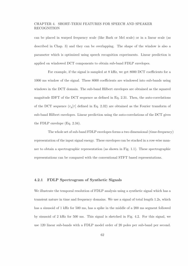
CHAPTER 4. SHORT-TERM FEATURES FOR SPEECH AND SPEAKERRECOGNITION
can be placed in warped frequency scale (like Bark or Mel scale) or in a linear scale (as
described in Chap. 3) and they can be overlapping. The shape of the window is also a
parameter which is optimized using speech recognition experiments. Linear prediction is
applied on windowed DCT components to obtain sub-band FDLP envelopes.
For example, if the signal is sampled at 8 kHz, we get 8000 DCT coefficients for a
1000 ms window of the signal. These 8000 coefficients are windowed into sub-bands using
windows in the DCT domain. The sub-band Hilbert envelopes are obtained as the squared
magnitude IDFT of the DCT sequence as defined in Eq. 2.31. Then, the auto-correlations
of the DCT sequence (ry[τ ] defined in Eq. 2.32) are obtained as the Fourier transform of
sub-band Hilbert envelopes. Linear prediction using the auto-correlations of the DCT gives
the FDLP envelope (Eq. 2.34).
The whole set of sub-band FDLP envelopes forms a two dimensional (time-frequency)
representation of the input signal energy. These envelopes can be stacked in a row-wise man-
ner to obtain a spectrographic representation (as shown in Fig. 1.1). These spectrographic
representations can be compared with the conventional STFT based representations.
4.2.1 FDLP Spectrogram of Synthetic Signals
We illustrate the temporal resolution of FDLP analysis using a synthetic signal which has a
transient nature in time and frequency domains. We use a signal of total length 1.2s, which
has a sinusoid of 1 kHz for 500 ms, has a spike in the middle of a 200 ms segment followed
by sinusoid of 2 kHz for 500 ms. This signal is sketched in Fig. 4.2. For this signal, we
use 120 linear sub-bands with a FDLP model order of 20 poles per sub-band per second.
62
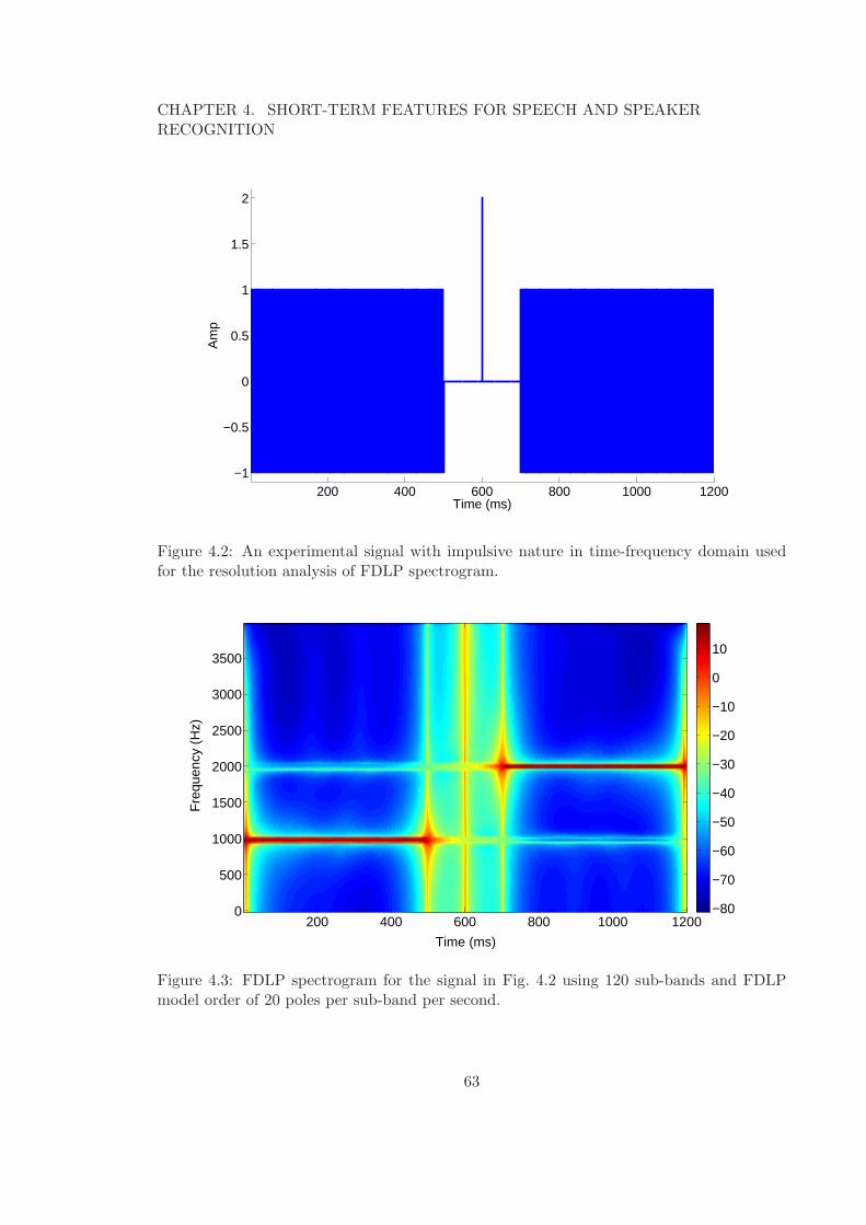
CHAPTER 4. SHORT-TERM FEATURES FOR SPEECH AND SPEAKERRECOGNITION
200 400 600 800 1000 1200−1
−0.5
0
0.5
1
1.5
2
Time (ms)
Am
p
Figure 4.2: An experimental signal with impulsive nature in time-frequency domain usedfor the resolution analysis of FDLP spectrogram.
Time (ms)
Fre
quen
cy (
Hz)
200 400 600 800 1000 1200
3500
3000
2500
2000
1500
1000
500
0 −80
−70
−60
−50
−40
−30
−20
−10
0
10
Figure 4.3: FDLP spectrogram for the signal in Fig. 4.2 using 120 sub-bands and FDLPmodel order of 20 poles per sub-band per second.
63
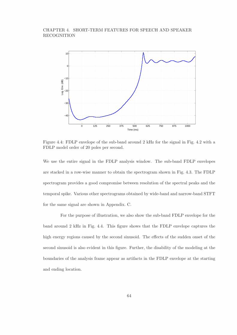
CHAPTER 4. SHORT-TERM FEATURES FOR SPEECH AND SPEAKERRECOGNITION
0 125 250 375 500 625 750 875 1000
−40
−30
−20
−10
0
10
Time (ms)
Log.
Env
. (dB
)
Figure 4.4: FDLP envelope of the sub-band around 2 kHz for the signal in Fig. 4.2 with aFDLP model order of 20 poles per second.
We use the entire signal in the FDLP analysis window. The sub-band FDLP envelopes
are stacked in a row-wise manner to obtain the spectrogram shown in Fig. 4.3. The FDLP
spectrogram provides a good compromise between resolution of the spectral peaks and the
temporal spike. Various other spectrograms obtained by wide-band and narrow-band STFT
for the same signal are shown in Appendix. C.
For the purpose of illustration, we also show the sub-band FDLP envelope for the
band around 2 kHz in Fig. 4.4. This figure shows that the FDLP envelope captures the
high energy regions caused by the second sinusoid. The effects of the sudden onset of the
second sinusoid is also evident in this figure. Further, the disability of the modeling at the
boundaries of the analysis frame appear as artifacts in the FDLP envelope at the starting
and ending location.
64
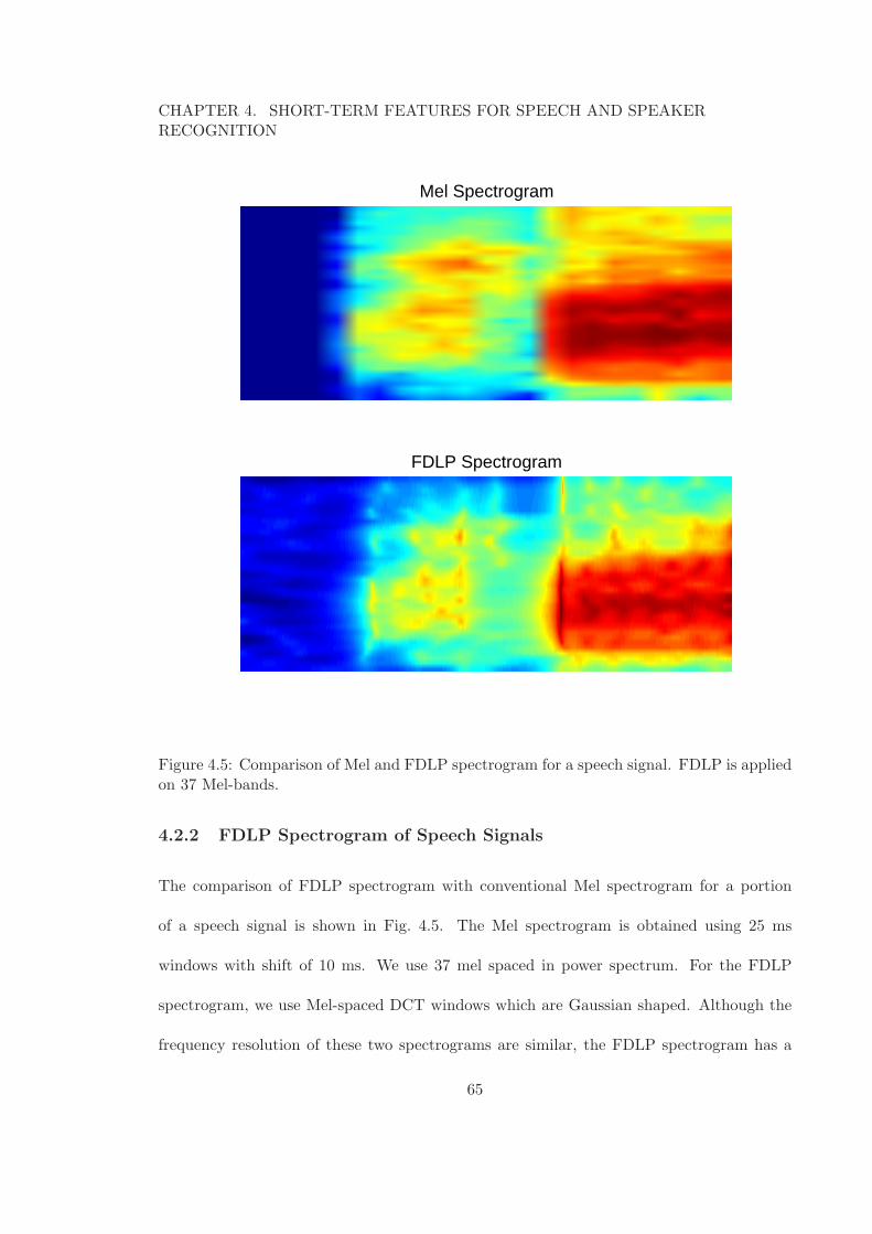
CHAPTER 4. SHORT-TERM FEATURES FOR SPEECH AND SPEAKERRECOGNITION
Mel Spectrogram
FDLP Spectrogram
Figure 4.5: Comparison of Mel and FDLP spectrogram for a speech signal. FDLP is appliedon 37 Mel-bands.
4.2.2 FDLP Spectrogram of Speech Signals
The comparison of FDLP spectrogram with conventional Mel spectrogram for a portion
of a speech signal is shown in Fig. 4.5. The Mel spectrogram is obtained using 25 ms
windows with shift of 10 ms. We use 37 mel spaced in power spectrum. For the FDLP
spectrogram, we use Mel-spaced DCT windows which are Gaussian shaped. Although the
frequency resolution of these two spectrograms are similar, the FDLP spectrogram has a
65
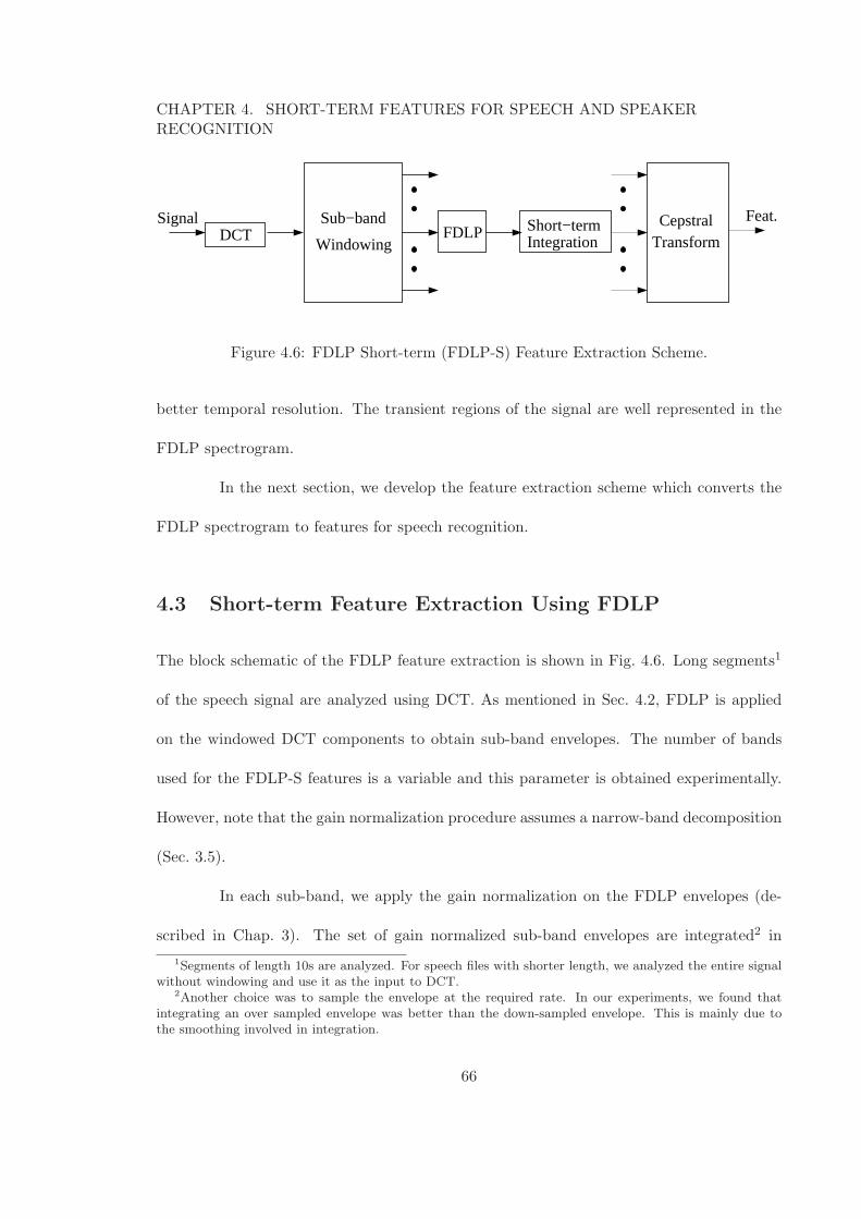
CHAPTER 4. SHORT-TERM FEATURES FOR SPEECH AND SPEAKERRECOGNITION
Windowing
Sub−bandFDLP Short−term
Feat.
TransformCepstral
DCTSignal
Integration
Figure 4.6: FDLP Short-term (FDLP-S) Feature Extraction Scheme.
better temporal resolution. The transient regions of the signal are well represented in the
FDLP spectrogram.
In the next section, we develop the feature extraction scheme which converts the
FDLP spectrogram to features for speech recognition.
4.3 Short-term Feature Extraction Using FDLP
The block schematic of the FDLP feature extraction is shown in Fig. 4.6. Long segments1
of the speech signal are analyzed using DCT. As mentioned in Sec. 4.2, FDLP is applied
on the windowed DCT components to obtain sub-band envelopes. The number of bands
used for the FDLP-S features is a variable and this parameter is obtained experimentally.
However, note that the gain normalization procedure assumes a narrow-band decomposition
(Sec. 3.5).
In each sub-band, we apply the gain normalization on the FDLP envelopes (de-
scribed in Chap. 3). The set of gain normalized sub-band envelopes are integrated2 in
1Segments of length 10s are analyzed. For speech files with shorter length, we analyzed the entire signalwithout windowing and use it as the input to DCT.
2Another choice was to sample the envelope at the required rate. In our experiments, we found thatintegrating an over sampled envelope was better than the down-sampled envelope. This is mainly due tothe smoothing involved in integration.
66
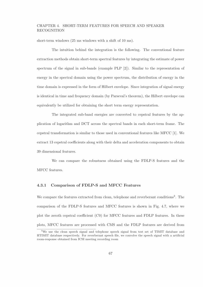
CHAPTER 4. SHORT-TERM FEATURES FOR SPEECH AND SPEAKERRECOGNITION
short-term windows (25 ms windows with a shift of 10 ms).
The intuition behind the integration is the following. The conventional feature
extraction methods obtain short-term spectral features by integrating the estimate of power
spectrum of the signal in sub-bands (example PLP [2]). Similar to the representation of
energy in the spectral domain using the power spectrum, the distribution of energy in the
time domain is expressed in the form of Hilbert envelope. Since integration of signal energy
is identical in time and frequency domain (by Parseval’s theorem), the Hilbert envelope can
equivalently be utilized for obtaining the short term energy representation.
The integrated sub-band energies are converted to cepstral features by the ap-
plication of logarithm and DCT across the spectral bands in each short-term frame. The
cepstral transformation is similar to those used in conventional features like MFCC [1]. We
extract 13 cepstral coefficients along with their delta and acceleration components to obtain
39 dimensional features.
We can compare the robustness obtained using the FDLP-S features and the
MFCC features.
4.3.1 Comparison of FDLP-S and MFCC Features
We compare the features extracted from clean, telephone and reverberant conditions3. The
comparison of the FDLP-S features and MFCC features is shown in Fig. 4.7, where we
plot the zeroth cepstral coefficient (C0) for MFCC features and FDLP features. In these
plots, MFCC features are processed with CMS and the FDLP features are derived from
3We use the clean speech signal and telephone speech signal from test set of TIMIT database andHTIMIT database respectively. For reverberant speech file, we convolve the speech signal with a artificialroom-response obtained from ICSI meeting recording room
67
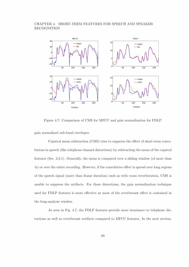
CHAPTER 4. SHORT-TERM FEATURES FOR SPEECH AND SPEAKERRECOGNITION
50 100 150 200
−40
−20
0
20
40MFCC
50 100 150 200
−40
−20
0
20
40
Frames
50 100 150 2000
5
10
15
FDLP
50 100 150 2000
5
10
15
Frames
clean
tel.
clean
revb.
clean
tel.
clean
revb.
Figure 4.7: Comparison of CMS for MFCC and gain normalization for FDLP.
gain normalized sub-band envelopes.
Cepstral mean subtraction (CMS) tries to suppress the effect of short-term convo-
lutions in speech (like telephone channel distortions) by subtracting the mean of the cepstral
features (Sec. 3.3.1). Generally, the mean is computed over a sliding window (of more than
1s) or over the entire recording. However, if the convolutive effect is spread over long regions
of the speech signal (more than frame duration) such as with room reverberation, CMS is
unable to suppress the artifacts. For these distortions, the gain normalization technique
used for FDLP features is more effective as most of the reverberant effect is contained in
the long-analysis window.
As seen in Fig. 4.7, the FDLP features provide more invariance to telephone dis-
tortions as well as reverberant artifacts compared to MFCC features. In the next section,
68
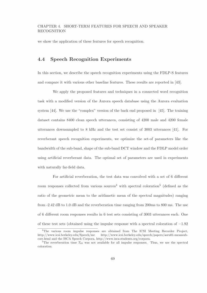
CHAPTER 4. SHORT-TERM FEATURES FOR SPEECH AND SPEAKERRECOGNITION
we show the application of these features for speech recognition.
4.4 Speech Recognition Experiments
In this section, we describe the speech recognition experiments using the FDLP-S features
and compare it with various other baseline features. These results are reported in [43].
We apply the proposed features and techniques in a connected word recognition
task with a modified version of the Aurora speech database using the Aurora evaluation
system [44]. We use the “complex” version of the back end proposed in [45]. The training
dataset contains 8400 clean speech utterances, consisting of 4200 male and 4200 female
utterances downsampled to 8 kHz and the test set consist of 3003 utterances [41]. For
reverberant speech recognition experiments, we optimize the set-of parameters like the
bandwidth of the sub-band, shape of the sub-band DCT window and the FDLP model order
using artificial reverberant data. The optimal set of parameters are used in experiments
with naturally far-field data.
For artificial reverberation, the test data was convolved with a set of 6 different
room responses collected from various sources4 with spectral coloration5 (defined as the
ratio of the geometric mean to the arithmetic mean of the spectral magnitudes) ranging
from -2.42 dB to 1.0 dB and the reverberation time ranging from 200ms to 800 ms. The use
of 6 different room responses results in 6 test sets consisting of 3003 utterances each. One
of these test sets (obtained using the impulse response with a spectral coloration of −1.92
4The various room impulse responses are obtained from The ICSI Meeting Recorder Project,http://www.icsi.berkeley.edu/Speech/mr http://www.icsi.berkeley.edu/speech/papers/asru01-meansub-corr.html and the ISCA Speech Corpora, http://www.isca-students.org/corpora.
5The reverberation time T60 was not available for all impulse responses. Thus, we use the spectralcoloration.
69

CHAPTER 4. SHORT-TERM FEATURES FOR SPEECH AND SPEAKERRECOGNITION
Features Clean Speech Revb. Speech
PLP 99.7 80.1
FDLP-MEL-Gauss-Without-Norm. 99.7 78.7
FDLP-MEL-Gauss-Gain-Norm. 99.5 85.3
FDLP-MEL-Rect-Gain-Norm. 99.4 89.1
FDLP-UNF-Rect-Gain-Norm. 99.2 89.5
Table 4.1: Word Accuracies (%) for clean and reverberant speech with various FDLP featureconfigurations.)
dB) is used to investigate the effect of varying the number of frequency sub-bands.
In the following sub-sections we analyze the effect of various parameters in the
FDLP model on the output word recognition rate.
4.4.1 Effect of Gain Normalization
The first set of experiments compare the performance of FDLP based features with the
conventional features for clean input conditions. Here, we also investigate the effect of gain
normalization of the FDLP envelopes on the final recognition rate for clean and reverberant
speech.
Table 4.4.1 shows the word accuracies for baseline PLP features (PLP) and FDLP
features extracted using a Gaussian shaped mel-filter bank without and with the gain nor-
malization on the temporal envelopes (FDLP-MEL-Gauss-Without-Norm., FDLP-MEL-
Gauss-Gain-Norm. respectively) and using a rectangular shaped mel spaced filter bank
with gain normalization (FDLP-MEL-Rect-Gain-Norm). We also experiment with uni-
70
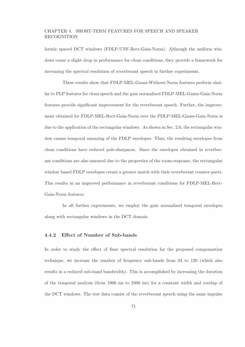
CHAPTER 4. SHORT-TERM FEATURES FOR SPEECH AND SPEAKERRECOGNITION
formly spaced DCT windows (FDLP-UNF-Rect-Gain-Norm). Although the uniform win-
dows cause a slight drop in performance for clean conditions, they provide a framework for
increasing the spectral resolution of reverberant speech in further experiments.
These results show that FDLP-MEL-Gauss-Without-Norm features perform simi-
lar to PLP features for clean speech and the gain normalized FDLP-MEL-Gauss-Gain-Norm
features provide significant improvement for the reverberant speech. Further, the improve-
ment obtained for FDLP-MEL-Rect-Gain-Norm over the FDLP-MEL-Gauss-Gain-Norm is
due to the application of the rectangular windows. As shown in Sec. 2.6, the rectangular win-
dow causes temporal smearing of the FDLP envelopes. Thus, the resulting envelopes from
clean conditions have reduced pole-sharpness. Since the envelopes obtained in reverber-
ant conditions are also smeared due to the properties of the room-response, the rectangular
window based FDLP envelopes create a greater match with their reverberant counter-parts.
This results in an improved performance in reverberant conditions for FDLP-MEL-Rect-
Gain-Norm features.
In all further experiments, we employ the gain normalized temporal envelopes
along with rectangular windows in the DCT domain.
4.4.2 Effect of Number of Sub-bands
In order to study the effect of finer spectral resolution for the proposed compensation
technique, we increase the number of frequency sub-bands from 24 to 120 (which also
results in a reduced sub-band bandwidth). This is accomplished by increasing the duration
of the temporal analysis (from 1000 ms to 2400 ms) for a constant width and overlap of
the DCT windows. The test data consist of the reverberant speech using the same impulse
71
CHAPTER 4. SHORT-TERM FEATURES FOR SPEECH AND SPEAKERRECOGNITION
20 30 40 50 60 70 80 90 100 110 120
88
90
92
94
96
98
100
Number of Bands
Acc
urac
y
Clean
Revb. 300ms
Figure 4.8: Recognition accuracy as function of the number of sub-bands.
response as before. Fig. 4.8 shows the recognition accuracies for the FDLP features when
the number of sub-bands is varied. As shown here, the best performance in reverberant
conditions is obtained using 96 linear sub-bands.
For a fixed number of sub-bands, the bandwidth of the sub-bands can be varied keeping
the band-overlap constant [46]. This would help us study the effect of band-width. The
narrow sub-band decomposition means that the modulation extent of the corresponding
modulation spectrum reduces (given by half of bandwidth of the sub-band). As seen in
Fig. 4.9, when the bandwidth reduces, the robustness in reverberant environment improves
significantly while the performance in clean conditions degrades moderately.
From these experiments, we find that increasing the frequency resolution strength-
ens the validity of the assumptions made for the gain normalization technique (Sec. 3.5)
72

CHAPTER 4. SHORT-TERM FEATURES FOR SPEECH AND SPEAKERRECOGNITION
50 75 100 125 150
50
60
70
80
90
100
Bandwidth
Acc
urac
y
Clean
Revb. 300ms
Revb. 700ms
Figure 4.9: Word recognition accuracy as function of the bandwidth of the sub-band forclean and two types of reverberant data.
and hence, significantly improves the recognition accuracies in reverberant conditions. In
the rest of the experiments, we use a 96 band decomposition with a bandwidth of 100 Hz.
4.4.3 Effect of FDLP Model Order
In these experiments, we investigate the effect of FDLP model order on the performance in
reverberant conditions [46]. When speech is corrupted by room reverberation, the sub-band
envelopes are smeared in time. The degree of smearing is determined by the reverberation
time (T60). In this case, higher order FDLP results in the estimation of large number of
signal peaks which are well represented in reverberant conditions. On the other hand, a
73
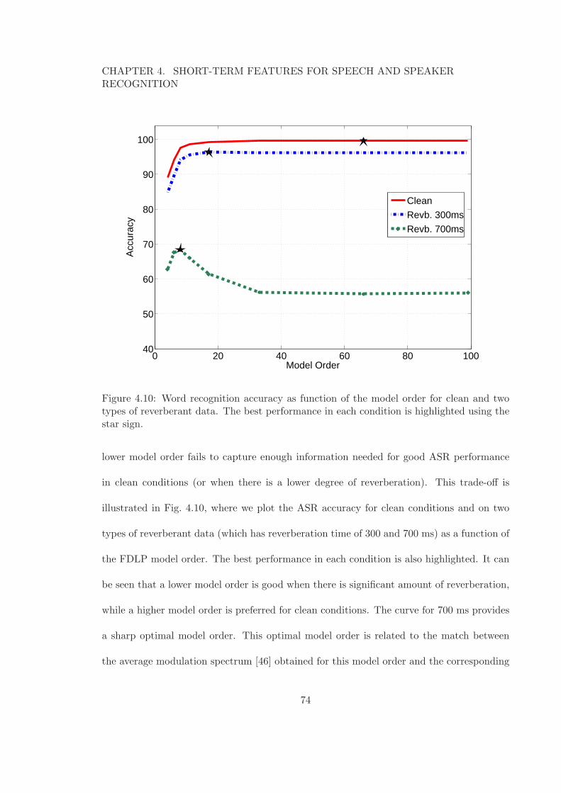
CHAPTER 4. SHORT-TERM FEATURES FOR SPEECH AND SPEAKERRECOGNITION
0 20 40 60 80 10040
50
60
70
80
90
100
Model Order
Acc
urac
y
Clean
Revb. 300ms
Revb. 700ms
Figure 4.10: Word recognition accuracy as function of the model order for clean and twotypes of reverberant data. The best performance in each condition is highlighted using thestar sign.
lower model order fails to capture enough information needed for good ASR performance
in clean conditions (or when there is a lower degree of reverberation). This trade-off is
illustrated in Fig. 4.10, where we plot the ASR accuracy for clean conditions and on two
types of reverberant data (which has reverberation time of 300 and 700 ms) as a function of
the FDLP model order. The best performance in each condition is also highlighted. It can
be seen that a lower model order is good when there is significant amount of reverberation,
while a higher model order is preferred for clean conditions. The curve for 700 ms provides
a sharp optimal model order. This optimal model order is related to the match between
the average modulation spectrum [46] obtained for this model order and the corresponding
74
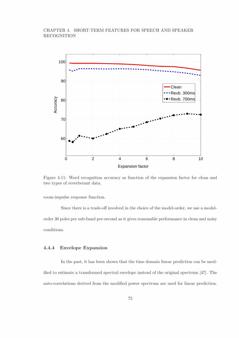
CHAPTER 4. SHORT-TERM FEATURES FOR SPEECH AND SPEAKERRECOGNITION
0 2 4 6 8 10
60
70
80
90
100
Expansion factor
Acc
urac
y
Clean
Revb. 300ms
Revb. 700ms
Figure 4.11: Word recognition accuracy as function of the expansion factor for clean andtwo types of reverberant data.
room-impulse response function.
Since there is a trade-off involved in the choice of the model-order, we use a model-
order 30 poles per sub-band per-second as it gives reasonable performance in clean and noisy
conditions.
4.4.4 Envelope Expansion
In the past, it has been shown that the time domain linear prediction can be mod-
ified to estimate a transformed spectral envelope instead of the original spectrum [47]. The
auto-correlations derived from the modified power spectrum are used for linear prediction.
75
CHAPTER 4. SHORT-TERM FEATURES FOR SPEECH AND SPEAKERRECOGNITION
In FDLP framework, spectral auto-correlations can be derived from transformed Hilbert
envelopes [46], where the transformation here corresponds to raising the original Hilbert
envelope to a power r. When the Hilbert envelope is compressed (r < 1), the resulting
model tends to approximate the valleys of the envelope better [47]. However, expansion of
the envelopes (r > 1) results in enhanced modeling of the peaks of the envelope.
We apply the transform linear prediction in FDLP and derive features for ASR.
When speech is corrupted by room reverberation, the high energy peaks (where the signal
to reverberant component ratio is high) can be more robustly estimated as compared to the
valleys of the envelope. Thus, FDLP features derived using expanded envelopes (r > 1) are
more robust in reverberant environments. This is illustrated in Fig. 4.11, where we plot the
ASR accuracy for clean conditions as well as the two reverberant conditions as function of
the the expansion factor r.
In these experiments, the envelope expansion provides significant improvements in
reverberant conditions. This also illustrates the advantage of all-pole modeling using FDLP.
Since the AR model estimates the peaks with high accuracy, these estimates are relatively
well preserved in noisy conditions.
The envelope expansion moderately reduces the performance in clean conditions.
In the remaining experiments, we do not use envelope expansion.
4.4.5 Results on Artificial Reverberation
In Fig. 4.12, the results for the proposed FDLP-S technique are compared with those ob-
tained for several other robust feature extraction techniques proposed for reverberant ASR
namely CMS [39] (Sec. 3.3.1), LTLSS [41] (Sec. 3.3.3) and LDMN [40] (Sec. 3.3.2). This is
76

CHAPTER 4. SHORT-TERM FEATURES FOR SPEECH AND SPEAKERRECOGNITION
−2.4 −2.3 −2.1 −1.9 −1.6 −1.0
30
40
50
60
70
80
90
100
Spectral Coloration (dB)
Acc
urac
y
FDLP
LTLSS
LDMN
CMS
PLP
Figure 4.12: Comparison of word recognition accuracies (%) using different techniques using6 artificial room responses.
done for the 6 different room impulse responses.
In our LTLSS experiments, we calculated the means independently for each indi-
vidual utterance (which differs from the approach of grouping multiple utterances for the
same speaker described in [41]) using a shorter analysis window of 32 ms, with a shift of
8 ms. For the FDLP features, we fix the number of sub-bands to 96. For the various
room responses, the proposed FDLP-S features, on the average, provide a relative error
improvement of 24% over the other feature extraction techniques considered. The relative
improvements are similar for the different room responses, although the absolute improve-
ments are higher for room impulse responses with higher spectral coloration (Fig. 4.12).
77

CHAPTER 4. SHORT-TERM FEATURES FOR SPEECH AND SPEAKERRECOGNITION
Channel PLP CMS LDMN LTLSS FDLP
Channel E 68.1 71.2 73.2 74.0 85.2
Channel F 75.5 77.4 80.4 81.0 88.1
Channel 6 74.1 78.3 80.9 81.1 89.6
Channel 7 58.6 67.6 70.5 71.0 84.9
Avg. 71.6 73.6 76.3 76.8 87
Table 4.2: Word Accuracies (%) using different feature extraction techniques on far-fieldmicrophone speech
4.4.6 Results on Natural Far-Field Reverberation
In order to investigate the performance of the proposed feature extraction for naturally
reverberant speech in background noise, we perform experiments on a a set of connected
digits recorded in a meeting room [48]. These experiments are performed on the digits
corpus recorded using far-field microphones as part of the ICSI Meeting task6. The corpus
consists of four sets of 2790 utterances each. Each of these sets correspond to speech recorded
simultaneously using four different far-field microphones. Each of these sets contain 9169
digits similar to those found in TIDIGITS corpus. We use the HMM models trained with
the clean speech from earlier experiments.
Table 4.4.5 shows the word accuracies for the different feature extraction techniques
using the far-field test data, where we obtain a relative error improvement of about 43%
over the other feature extraction techniques.
The experiments on speech recognition task showed that the proposed features
6The ICSI Meeting Recorder Project, http://www.icsi.berkeley.edu/Speech/mr
78
CHAPTER 4. SHORT-TERM FEATURES FOR SPEECH AND SPEAKERRECOGNITION
provide significant improvements for artificial and natural reverberation. In the next section,
we perform experiments on a speaker verification task.
4.5 Speaker Verification Experiments
In this section, we describe the speaker recognition experiments performed using the FDLP-
S features [49].
4.5.1 Experimental set-up
The input speech features are feature warped [50], which is technique of normalizing the
distribution of the features. The input feature distribution is warped to a Gaussian dis-
tribution with zero-mean and unit variance. The warping of the features improves the
performance in speaker verification [50].
We use a GMM-UBM based speaker verification system [51]. The features are used
to train a 512 component GMM on the development data. Once the UBM is trained, the
mixture component means are maximum-a-posteriori (MAP) adapted and concatenated to
form supervectors [52]. These supervectors characterize the speaker model for the target
speaker.
In order to remove the effect of channel on the speaker models, nuisance attribute
projection (NAP) is applied on the supervectors. The NAP technique attempts to remove
directions which correspond to large intra speaker variability (like session variability) which
are caused by channel variations [53]. In the NAP method, the high-variance principal
components correspond to the channel (nuisance) space and low-variance components cor-
79
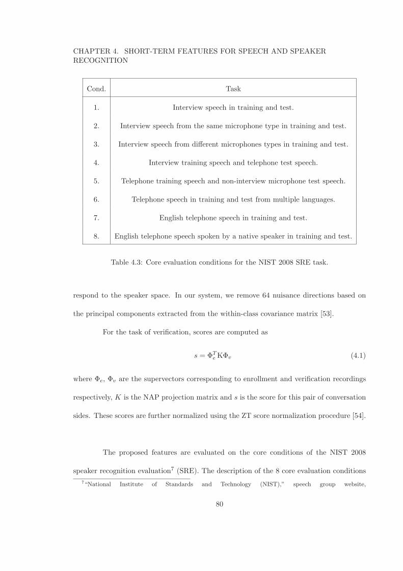
CHAPTER 4. SHORT-TERM FEATURES FOR SPEECH AND SPEAKERRECOGNITION
Cond. Task
1. Interview speech in training and test.
2. Interview speech from the same microphone type in training and test.
3. Interview speech from different microphones types in training and test.
4. Interview training speech and telephone test speech.
5. Telephone training speech and non-interview microphone test speech.
6. Telephone speech in training and test from multiple languages.
7. English telephone speech in training and test.
8. English telephone speech spoken by a native speaker in training and test.
Table 4.3: Core evaluation conditions for the NIST 2008 SRE task.
respond to the speaker space. In our system, we remove 64 nuisance directions based on
the principal components extracted from the within-class covariance matrix [53].
For the task of verification, scores are computed as
s = ΦTe KΦv (4.1)
where Φe, Φv are the supervectors corresponding to enrollment and verification recordings
respectively, K is the NAP projection matrix and s is the score for this pair of conversation
sides. These scores are further normalized using the ZT score normalization procedure [54].
The proposed features are evaluated on the core conditions of the NIST 2008
speaker recognition evaluation7 (SRE). The description of the 8 core evaluation conditions
7“National Institute of Standards and Technology (NIST),” speech group website,
80
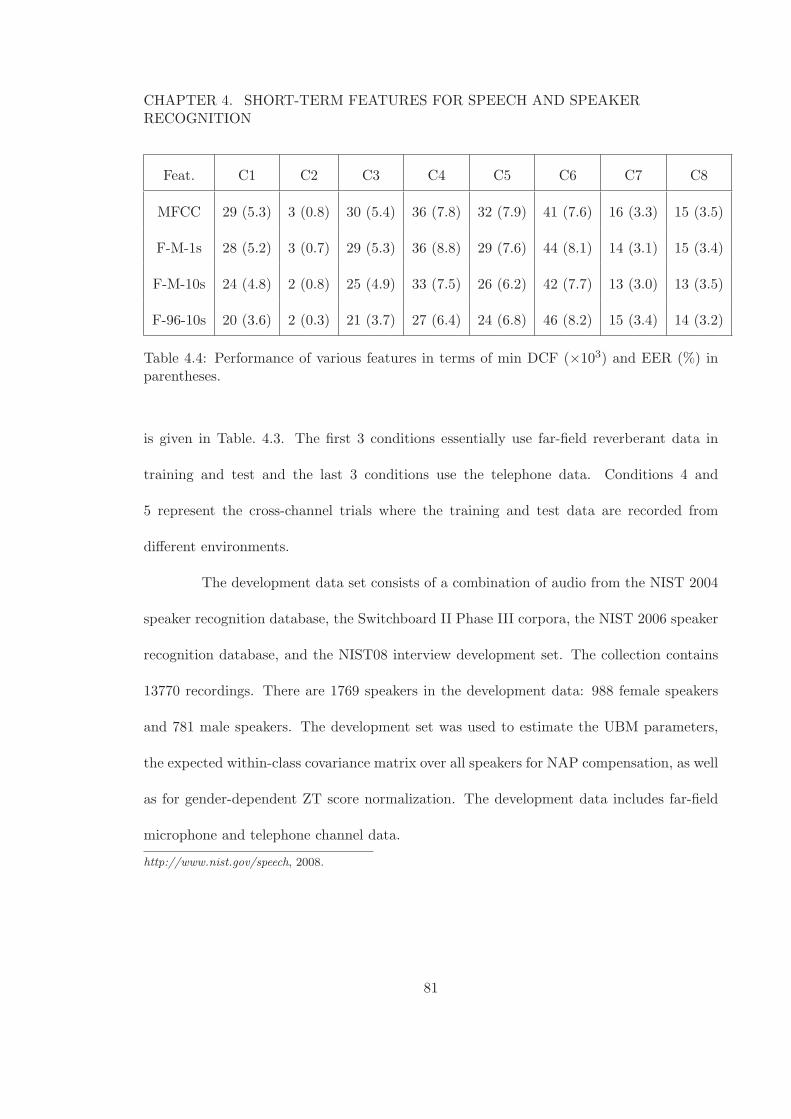
CHAPTER 4. SHORT-TERM FEATURES FOR SPEECH AND SPEAKERRECOGNITION
Feat. C1 C2 C3 C4 C5 C6 C7 C8
MFCC 29 (5.3) 3 (0.8) 30 (5.4) 36 (7.8) 32 (7.9) 41 (7.6) 16 (3.3) 15 (3.5)
F-M-1s 28 (5.2) 3 (0.7) 29 (5.3) 36 (8.8) 29 (7.6) 44 (8.1) 14 (3.1) 15 (3.4)
F-M-10s 24 (4.8) 2 (0.8) 25 (4.9) 33 (7.5) 26 (6.2) 42 (7.7) 13 (3.0) 13 (3.5)
F-96-10s 20 (3.6) 2 (0.3) 21 (3.7) 27 (6.4) 24 (6.8) 46 (8.2) 15 (3.4) 14 (3.2)
Table 4.4: Performance of various features in terms of min DCF (×103) and EER (%) inparentheses.
is given in Table. 4.3. The first 3 conditions essentially use far-field reverberant data in
training and test and the last 3 conditions use the telephone data. Conditions 4 and
5 represent the cross-channel trials where the training and test data are recorded from
different environments.
The development data set consists of a combination of audio from the NIST 2004
speaker recognition database, the Switchboard II Phase III corpora, the NIST 2006 speaker
recognition database, and the NIST08 interview development set. The collection contains
13770 recordings. There are 1769 speakers in the development data: 988 female speakers
and 781 male speakers. The development set was used to estimate the UBM parameters,
the expected within-class covariance matrix over all speakers for NAP compensation, as well
as for gender-dependent ZT score normalization. The development data includes far-field
microphone and telephone channel data.
http://www.nist.gov/speech, 2008.
81

CHAPTER 4. SHORT-TERM FEATURES FOR SPEECH AND SPEAKERRECOGNITION
4.5.2 Speaker Recognition Results
The baseline features are 39 dimensional MFCC features [1] containing 13 cepstral
coefficients, their delta and acceleration components. These features are computed with a
frame shift of 10ms. We use 37 Mel-filters for the baseline features.
The FDLP features are used in 3 configurations. All configurations use the gain
normalization technique on the FDLP envelopes. F-M-1s corresponds to features derived
from temporal envelopes directly on the mel-bands (37 mel bands instead of 96 linear bands).
These features use a temporal analysis window of 1s on the input speech (and hence, a 1s
window for the gain normalization as well). F-M-10s also uses mel-band temporal envelopes
obtained from an input analysis window of 10s. F-96-10s features use a 10s analysis window
and derive temporal envelopes in 96 linear sub-bands. Gain normalization is applied on the
sub-band envelopes of all these features.
The speaker verification results for the various feature extraction techniques are
reported in Table 4.4. F-M-1s features provide performances similar to the baseline MFCC
features. When the analysis window is increased to 10s, there is a relative performance
improvement of about 15% on almost all the conditions. Furthermore, applying an initial
sub-band analysis of 96 bands provides significant improvements for the interview mic con-
ditions (relatively about 20-30% over the baseline system). This is due to the application of
gain normalization on longer analysis windows in narrow sub-bands which validates the first
order approximation made in the technique (Sec. 3.5). A drop in performance is observed
for Cond. 6 which may be attributed to the use of different languages in training and test
conditions (where the use of longer context degrades the performance).
82
CHAPTER 4. SHORT-TERM FEATURES FOR SPEECH AND SPEAKERRECOGNITION
4.6 Chapter Summary
In this Chapter, we have developed the short-term features from FDLP spectro-
gram for speech recognition and speaker verification. We begin with the two-dimensional
spectrographic representation using sub-band FDLP envelopes (Sec. 4.2). Then, we de-
scribe the FDLP-S feature extraction scheme in Sec. 4.3. The application of these features
for recognition experiments is reported in Sec. 4.4 and Sec. 4.5.
Recognition experiments gave the following conclusions -
1. Gain normalization results in improvements in recognition performance in reverberant
conditions without severely degrading the performance in matched conditions.
2. The assumption used in gain normalization are validated by the use of long-term
analysis in narrow bands.
3. A trade-off appears in the model order selection for representation of clean and rever-
berant speech.
4. Speech recognition experiments show the improvements in mis-match train/test condi-
tions where as the speaker recognition experiments are done with matched conditions.
The FDLP-S features provide significant improvements in both conditions compared
to baseline features.
Although the FDLP-S features are easily applicable to conventional systems (like
HMM-GMM), the integration in time-domain using short-term segments inherently reduces
the temporal resolution. In fact, the temporal resolution of the FDLP-S features are similar
83
CHAPTER 4. SHORT-TERM FEATURES FOR SPEECH AND SPEAKERRECOGNITION
to the conventional STFT based approaches. Therefore, there is need to derive alternate
representation which can utilize the higher resolution present in the FDLP envelopes.
In the next chapter, we introduce the modulation feature extraction using FDLP
representation (FDLP-M features) which are derived from syllable length segments without
any integration. The modulation representation makes use of the higher temporal resolution
in FDLP. These are used for phoneme recognition in noisy environments.
84
Chapter 5
Modulation Features Using FDLP
5.1 Chapter Outline
In this chapter, we develop the modulation feature extraction scheme. These
features are extracted from syllable-length segments of the sub-band FDLP envelopes.
These features can make use of the higher temporal resolution found in the FDLP analysis
(Sec. 4.2). The sub-band FDLP envelopes are compressed using static and dynamic com-
pression. These are converted to modulation spectral components and used as features for
phoneme recognition task.
The remainder of the chapter is organized as follows. In Sec. 5.2, we describe the
modulation feature extraction using FDLP spectrogram. The application of these features
for phoneme recognition task in clean conditions is reported in Sec. 5.3. The noise com-
pensation procedure which attempts to derive robust envelopes in additive noise conditions
is developed in Sec. 5.4. Phoneme recognition experiments in noisy speech is detailed in
Sec. 5.5. The analysis of the relative contribution from various stages in the modulation
85
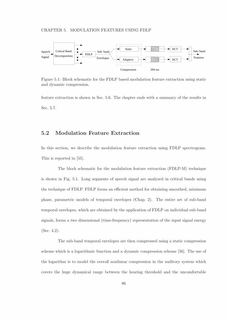
CHAPTER 5. MODULATION FEATURES USING FDLP
...
.
Static
Adaptive
Compression
Sub−band
Envelopes
200 ms
FDLPCritical Band
Decomposition
Speech
SignalDCT
DCT
Features
Sub−band
Figure 5.1: Block schematic for the FDLP based modulation feature extraction using staticand dynamic compression.
feature extraction is shown in Sec. 5.6. The chapter ends with a summary of the results in
Sec. 5.7.
5.2 Modulation Feature Extraction
In this section, we describe the modulation feature extraction using FDLP spectrogram.
This is reported in [55].
The block schematic for the modulation feature extraction (FDLP-M) technique
is shown in Fig. 5.1. Long segments of speech signal are analyzed in critical bands using
the technique of FDLP. FDLP forms an efficient method for obtaining smoothed, minimum
phase, parametric models of temporal envelopes (Chap. 2). The entire set of sub-band
temporal envelopes, which are obtained by the application of FDLP on individual sub-band
signals, forms a two dimensional (time-frequency) representation of the input signal energy
(Sec. 4.2).
The sub-band temporal envelopes are then compressed using a static compression
scheme which is a logarithmic function and a dynamic compression scheme [56]. The use of
the logarithm is to model the overall nonlinear compression in the auditory system which
covers the huge dynamical range between the hearing threshold and the uncomfortable
86
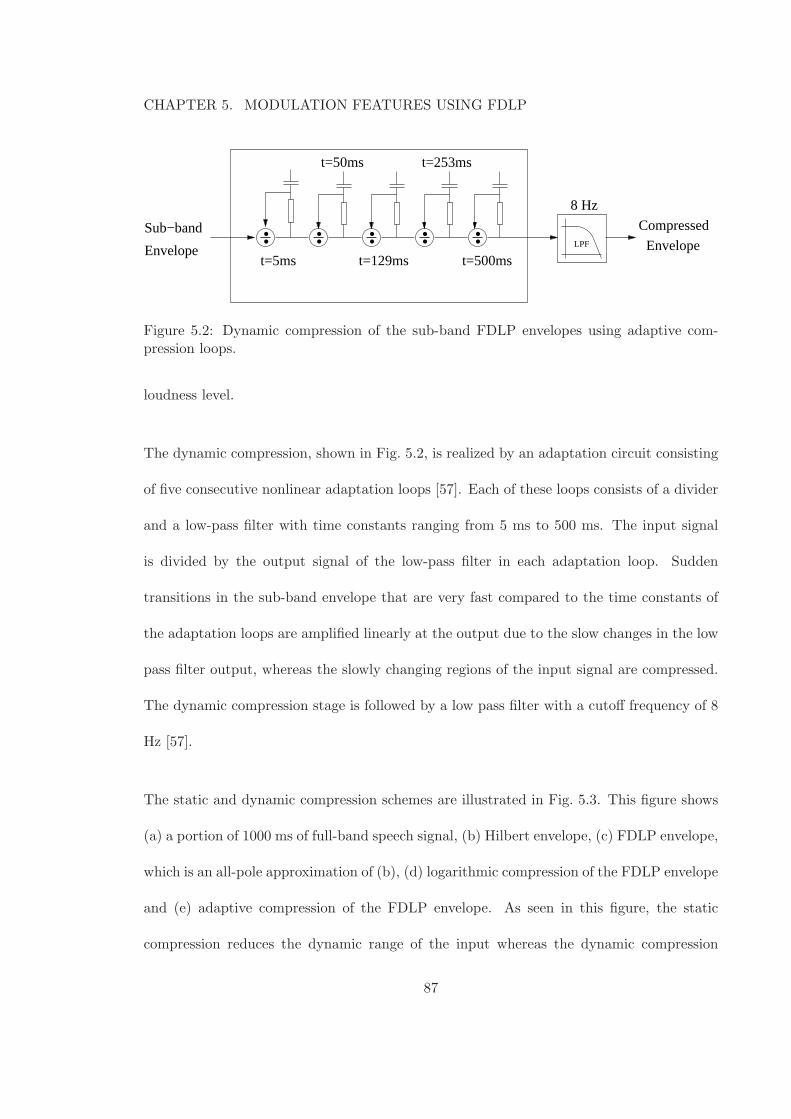
CHAPTER 5. MODULATION FEATURES USING FDLP
LPF
.. .. .. .. ..
t=5ms t=129ms t=500ms
t=50ms t=253ms
Compressed
8 Hz
Sub−bandEnvelopeEnvelope
Figure 5.2: Dynamic compression of the sub-band FDLP envelopes using adaptive com-pression loops.
loudness level.
The dynamic compression, shown in Fig. 5.2, is realized by an adaptation circuit consisting
of five consecutive nonlinear adaptation loops [57]. Each of these loops consists of a divider
and a low-pass filter with time constants ranging from 5 ms to 500 ms. The input signal
is divided by the output signal of the low-pass filter in each adaptation loop. Sudden
transitions in the sub-band envelope that are very fast compared to the time constants of
the adaptation loops are amplified linearly at the output due to the slow changes in the low
pass filter output, whereas the slowly changing regions of the input signal are compressed.
The dynamic compression stage is followed by a low pass filter with a cutoff frequency of 8
Hz [57].
The static and dynamic compression schemes are illustrated in Fig. 5.3. This figure shows
(a) a portion of 1000 ms of full-band speech signal, (b) Hilbert envelope, (c) FDLP envelope,
which is an all-pole approximation of (b), (d) logarithmic compression of the FDLP envelope
and (e) adaptive compression of the FDLP envelope. As seen in this figure, the static
compression reduces the dynamic range of the input whereas the dynamic compression
87
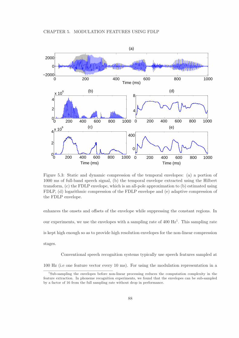
CHAPTER 5. MODULATION FEATURES USING FDLP
0 200 400 600 800 10000
2
4
x 106 (b)
0 200 400 600 800 1000−2000
0
2000
Time (ms)
(a)
0 200 400 600 800 1000
4
8(d)
0 200 400 600 800 10000
2
4x 10⁶
Time (ms)
(c)
0 200 400 600 800 1000
0
400
Time (ms)
(e)
Figure 5.3: Static and dynamic compression of the temporal envelopes: (a) a portion of1000 ms of full-band speech signal, (b) the temporal envelope extracted using the Hilberttransform, (c) the FDLP envelope, which is an all-pole approximation to (b) estimated usingFDLP, (d) logarithmic compression of the FDLP envelope and (e) adaptive compression ofthe FDLP envelope.
enhances the onsets and offsets of the envelope while suppressing the constant regions. In
our experiments, we use the envelopes with a sampling rate of 400 Hz1. This sampling rate
is kept high enough so as to provide high resolution envelopes for the non-linear compression
stages.
Conventional speech recognition systems typically use speech features sampled at
100 Hz (i.e one feature vector every 10 ms). For using the modulation representation in a
1Sub-sampling the envelopes before non-linear processing reduces the computation complexity in thefeature extraction. In phoneme recognition experiments, we found that the envelopes can be sub-sampledby a factor of 16 from the full sampling rate without drop in performance.
88
CHAPTER 5. MODULATION FEATURES USING FDLP
conventional system, the compressed temporal envelopes are divided into 200 ms segments
with a shift of 10 ms. Discrete Cosine Transform (DCT) of both the static and the dynamic
segments of temporal envelope yields the static and the dynamic modulation spectrum
respectively. We use 14 modulation frequency components from each cosine transform,
yielding modulation spectrum in the 0 − 35 Hz region with a resolution of 2.5 Hz. This
choice of a parameters is a result of series of phoneme recognition experiments reported in
Sec. 5.3.
In the next section, we describe the phoneme recognition experiments using these
features.
5.3 Phoneme Recognition Setup
5.3.1 MLP Based Phoneme Recognition
The phoneme recognition system is based on the Hidden Markov Model - Artificial Neural
Network (HMM-ANN) paradigm [58]. The multi-layer perceptron (MLP) estimates the
posterior probability of phonemes given the acoustic evidence P (qt = i|xt), where qt denotes
the phoneme index at frame t, xt denotes the feature vector. The relation between the
posterior probability P (qt = i|xt) and the likelihood P (xt|qt = i) is given by the Bayes rule,
p(xt|qt = i)
p(xt)=P (qt = i|xt)P (qt = i)
. (5.1)
It is shown in [58] that the neural network with sufficient capacity and trained on
enough data estimates the true Bayesian a-posteriori probability. The scaled likelihood in
an HMM state is given by Eq. 5.1, where we assume equal prior probability P (qt = i) for
89
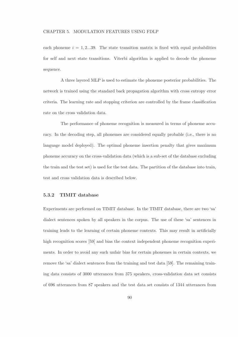
CHAPTER 5. MODULATION FEATURES USING FDLP
each phoneme i = 1, 2...39. The state transition matrix is fixed with equal probabilities
for self and next state transitions. Viterbi algorithm is applied to decode the phoneme
sequence.
A three layered MLP is used to estimate the phoneme posterior probabilities. The
network is trained using the standard back propagation algorithm with cross entropy error
criteria. The learning rate and stopping criterion are controlled by the frame classification
rate on the cross validation data.
The performance of phoneme recognition is measured in terms of phoneme accu-
racy. In the decoding step, all phonemes are considered equally probable (i.e., there is no
language model deployed). The optimal phoneme insertion penalty that gives maximum
phoneme accuracy on the cross-validation data (which is a sub-set of the database excluding
the train and the test set) is used for the test data. The partition of the database into train,
test and cross validation data is described below.
5.3.2 TIMIT database
Experiments are performed on TIMIT database. In the TIMIT database, there are two ‘sa’
dialect sentences spoken by all speakers in the corpus. The use of these ‘sa’ sentences in
training leads to the learning of certain phoneme contexts. This may result in artificially
high recognition scores [59] and bias the context independent phoneme recognition experi-
ments. In order to avoid any such unfair bias for certain phonemes in certain contexts, we
remove the ‘sa’ dialect sentences from the training and test data [59]. The remaining train-
ing data consists of 3000 utterances from 375 speakers, cross-validation data set consists
of 696 utterances from 87 speakers and the test data set consists of 1344 utterances from
90

CHAPTER 5. MODULATION FEATURES USING FDLP
168 speakers. The TIMIT database, which is hand-labeled using 61 labels is mapped to the
standard set of 39 phonemes [60]. We do not apply any speaker based normalization on the
input features.
In the TIMIT phoneme recognition system, the MLP consists of 1000 hidden
neurons, and 39 output neurons (with soft max non-linearity) representing the phoneme
classes.
5.3.3 CTS database
The conversation telephone speech (CTS) database consists of 300 hours of conver-
sational speech recorded over a telephone channel at 8 kHz [61]. The training data consists
of 250 hours of speech from 4538 speakers, cross-validation data set consists of 40 hours of
speech from 726 speakers and the test data set consists of 10 hours from 182 speakers. It
is labeled using 45 phonemes. The phoneme labels are obtained by force aligning the word
transcriptions to the previously trained HMM-GMM models [61].
Here, the MLP consists of 8270 hidden neurons, and 45 output neurons (with soft
max non-linearity) representing the phoneme classes.
5.3.4 Phoneme Recognition Results
In this section, we compare the phoneme recognition performance of FDLP-M
features with other modulation features and baseline PLP features. These results were first
reported in [62].
The baseline system for these experiments uses the conventional Perceptual Linear
Prediction (PLP) features [2] with a context of 9 frames [60] (351 dimensional features
91
CHAPTER 5. MODULATION FEATURES USING FDLP
PLP-9 Fepstrum MSG MRASTA FDLP-M
66.8 61.1 62.4 64.5 69.3
Table 5.1: Phoneme Recognition Accuracies (%) for PLP features and various modulationfeatures on TIMIT database.
denoted as PLP-9). In the past, some of the modulation feature techniques have been
used as additional sources of information by combining the modulation spectrum with
conventional short-term PLP or MFCC features (for example Fepstrum [63], MSG [23]).
However, in our experiments we report the recognition performance of the modulation
features independently without any combination. This is done in order to illustrate the use
of modulation spectrum as alternate representation compared to the conventional short-
term spectral features.
In our implementation, Fepstrum features consist of 5 modulation frequency com-
ponents in the 0 − 25 Hz range from 40 mel bands yielding 200 dimensional vector for
each frame. These features are dimensionality reduced to 60 dimensional features [63]. A
context of 9 frames gives a 540 dimensional feature vector at the input of the phoneme
recognition system. MSG features consist of 9 modulation components from 36 sub-bands
resulting in 324 dimensional features for every speech frame [23]. MRASTA features use 19
critical bands with 14 modulation filters. These are appended with frequency derivatives
yielding 504 dimensional features [22]. For the FDLP based modulation features, 21 critical
bands are used with 14 static modulation spectral components and 14 dynamic modulation
spectral components. This gives 588 dimensional features2 at the input vector.
2The number of modulation components derived is a parameter obtained by optimization using phonemerecognition experiments reported in next section.
92
CHAPTER 5. MODULATION FEATURES USING FDLP
Table 5.1 summarizes the results for the phoneme recognition experiments with
various modulation features. Among the past modulation approaches, MRASTA features
provide the best phoneme recognition performance. FDLP based features using static and
dynamic modulation spectrum provides a relative improvement of 7.5 % compared to the
baseline PLP features.
5.3.5 Effect of Various Parameters
The previous section showed that the proposed feature extraction provides promis-
ing results on TIMIT database. In-order to analyze the relative contribution of various
stages of the proposed feature extraction, we perform a set of phoneme recognition experi-
ments with different modifications to the proposed features. These modifications are:
Choice of AM demodulation
The proposed features use FDLP technique for AM demodulation of sub-band signals. As
mentioned in Sec. 1.2.1, other methods of AM demodulation have been used in the past.
We compare the phoneme recognition performance of FDLP approach with the half-wave
rectification technique [23] and the sub-band energy trajectory approach [22]. All the other
processing stages in the proposed features (like the sub-band decomposition, static and
dynamic modulation spectrum etc) are retained. These results are shown in Table 5.2. In
these experiments, FDLP based AM demodulation provides the best phoneme recognition.
93

CHAPTER 5. MODULATION FEATURES USING FDLP
AM Demodulation
Half-Wave Energy FDLP
67.0 67.7 69.3
Temporal Context (ms)
100 200 300 400
68.7 69.3 68.0 66.2
Modulation Extent (Hz)
15 25 35 45
67.1 69.1 69.3 69.1
Type of Modulation
Stat. Dyn. Stat. + Dyn.
67.9 64.6 69.3
Table 5.2: Phoneme Recognition Accuracies (%) for various modifications of the proposedfeature extraction technique.
Duration of Temporal Context
The temporal analysis window for the extraction of static and dynamic modulations is
modified in these experiments from 100 to 400 ms. This duration represents the contextual
information used in deriving modulation components3. FDLP based sub-band processing
is used and static and dynamic modulation features are derived. These results are shown
3This is different from the FDLP envelope computation window which is typically of the order of fewseconds. We window the FDLP envelope into segments with varying lengths (100-400 ms with a shift of10 ms). Within each segment, a temporal DCT is applied to obtain 14 static and 14 dynamic modulationcomponents.
94
CHAPTER 5. MODULATION FEATURES USING FDLP
in the second row of Table 5.2. It is interesting to note that the best phoneme recognition
performance is obtained for a context of 200 ms, which also corresponds to the average
syllabic rate of human speech.
Extent of Modulation Information
In these experiments, the extent of modulation spectrum used for feature extraction is varied
from 15-45 Hz. The duration of modulation analysis on the FDLP envelopes is fixed at 200
ms and the number of DCT coefficients is varied. Static and dynamic modulations are used
for phoneme recognition. These results, reported in the third row of Table 5.2, show that
the phoneme recognition performance peaks for a modulation content in the range 0-35 Hz
(14 DCT components from static and dynamic compression streams).
Type of Modulation Spectrum
As mentioned before, we derive modulation information from two types of envelope com-
pression scheme. Static modulations are derived using a logarithmic compression and the
dynamic modulations are derived using adaptive loops. FDLP envelope with a temporal
context of 200 ms is used for deriving the modulations in the range of 0-35 Hz. These
results are shown at the bottom of Table 5.2. The static modulation features provide good
phoneme recognition for fricatives and nasals (which is due to modeling property of the
signal peaks in static compression) whereas the dynamic modulation features provide good
performance for plosives and affricates (where the fine temporal fluctuations like onsets and
offsets carry the important phoneme classification information) [55]. Hence, the concate-
nating the feature streams results in considerable improvement in performance for most of
95
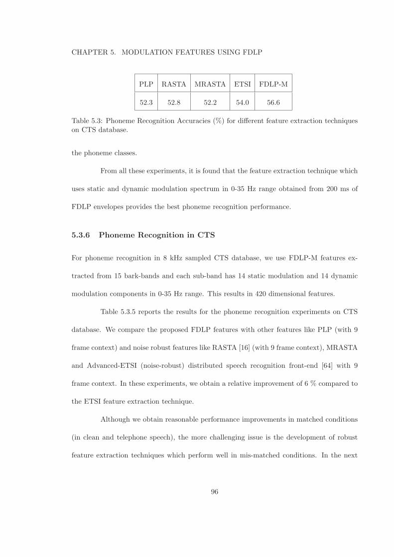
CHAPTER 5. MODULATION FEATURES USING FDLP
PLP RASTA MRASTA ETSI FDLP-M
52.3 52.8 52.2 54.0 56.6
Table 5.3: Phoneme Recognition Accuracies (%) for different feature extraction techniqueson CTS database.
the phoneme classes.
From all these experiments, it is found that the feature extraction technique which
uses static and dynamic modulation spectrum in 0-35 Hz range obtained from 200 ms of
FDLP envelopes provides the best phoneme recognition performance.
5.3.6 Phoneme Recognition in CTS
For phoneme recognition in 8 kHz sampled CTS database, we use FDLP-M features ex-
tracted from 15 bark-bands and each sub-band has 14 static modulation and 14 dynamic
modulation components in 0-35 Hz range. This results in 420 dimensional features.
Table 5.3.5 reports the results for the phoneme recognition experiments on CTS
database. We compare the proposed FDLP features with other features like PLP (with 9
frame context) and noise robust features like RASTA [16] (with 9 frame context), MRASTA
and Advanced-ETSI (noise-robust) distributed speech recognition front-end [64] with 9
frame context. In these experiments, we obtain a relative improvement of 6 % compared to
the ETSI feature extraction technique.
Although we obtain reasonable performance improvements in matched conditions
(in clean and telephone speech), the more challenging issue is the development of robust
feature extraction techniques which perform well in mis-matched conditions. In the next
96
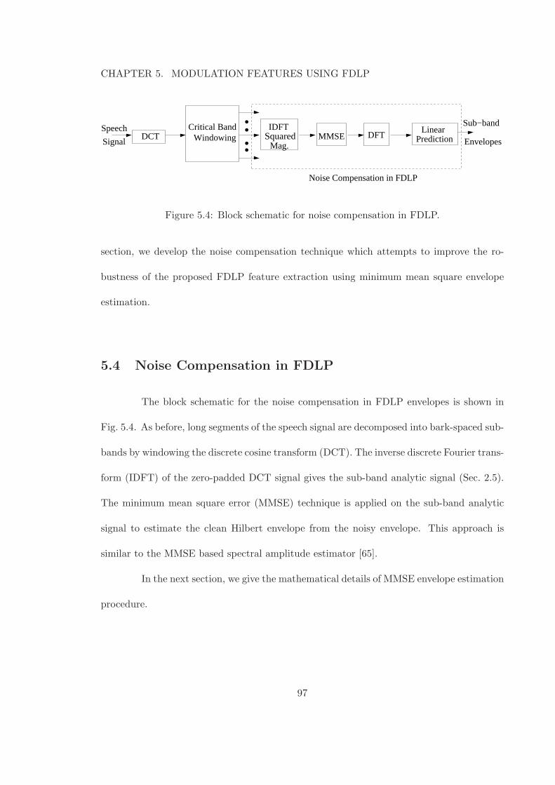
CHAPTER 5. MODULATION FEATURES USING FDLP
Squared....
WindowingCritical Band
DCTSpeech
Signal
IDFT
Mag.
LinearPredictionDFTMMSE
Sub−band
Envelopes
Noise Compensation in FDLP
Figure 5.4: Block schematic for noise compensation in FDLP.
section, we develop the noise compensation technique which attempts to improve the ro-
bustness of the proposed FDLP feature extraction using minimum mean square envelope
estimation.
5.4 Noise Compensation in FDLP
The block schematic for the noise compensation in FDLP envelopes is shown in
Fig. 5.4. As before, long segments of the speech signal are decomposed into bark-spaced sub-
bands by windowing the discrete cosine transform (DCT). The inverse discrete Fourier trans-
form (IDFT) of the zero-padded DCT signal gives the sub-band analytic signal (Sec. 2.5).
The minimum mean square error (MMSE) technique is applied on the sub-band analytic
signal to estimate the clean Hilbert envelope from the noisy envelope. This approach is
similar to the MMSE based spectral amplitude estimator [65].
In the next section, we give the mathematical details of MMSE envelope estimation
procedure.
97
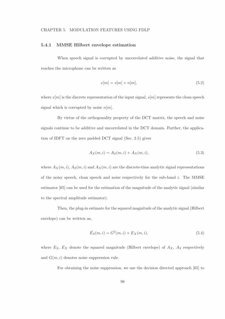
CHAPTER 5. MODULATION FEATURES USING FDLP
5.4.1 MMSE Hilbert envelope estimation
When speech signal is corrupted by uncorrelated additive noise, the signal that
reaches the microphone can be written as
x[m] = s[m] + n[m], (5.2)
where x[m] is the discrete representation of the input signal, s[m] represents the clean speech
signal which is corrupted by noise n[m].
By virtue of the orthogonality property of the DCT matrix, the speech and noise
signals continue to be additive and uncorrelated in the DCT domain. Further, the applica-
tion of IDFT on the zero padded DCT signal (Sec. 2.5) gives
AX(m, i) = AS(m, i) +AN (m, i), (5.3)
where AX(m, i), AS(m, i) and AN (m, i) are the discrete-time analytic signal representations
of the noisy speech, clean speech and noise respectively for the sub-band i. The MMSE
estimator [65] can be used for the estimation of the magnitude of the analytic signal (similar
to the spectral amplitude estimator).
Then, the plug-in estimate for the squared magnitude of the analytic signal (Hilbert
envelope) can be written as,
ES(m, i) = G2(m, i)× EX(m, i), (5.4)
where ES , EX denote the squared magnitude (Hilbert envelope) of AX , AS respectively
and G(m, i) denotes noise suppression rule.
For obtaining the noise suppression, we use the decision directed approach [65] to
98
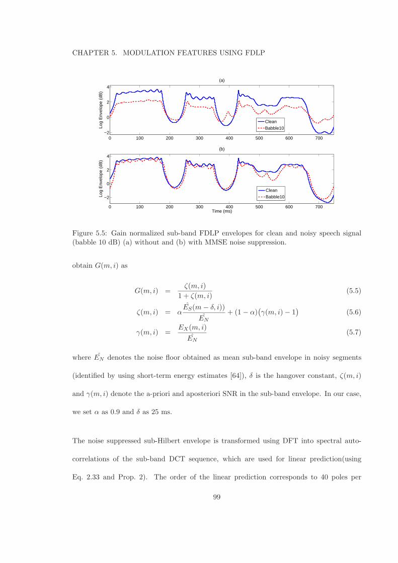
CHAPTER 5. MODULATION FEATURES USING FDLP
0 100 200 300 400 500 600 700−2
0
2
4
Log
Env
elop
e (d
B)
(a)
0 100 200 300 400 500 600 700
−2
0
2
4
(b)
Time (ms)
Log
Env
elop
e (d
B)
Clean
Babble10
Clean
Babble10
Figure 5.5: Gain normalized sub-band FDLP envelopes for clean and noisy speech signal(babble 10 dB) (a) without and (b) with MMSE noise suppression.
obtain G(m, i) as
G(m, i) =ζ(m, i)
1 + ζ(m, i)(5.5)
ζ(m, i) = αES(m− δ, i))
EN
+ (1− α)(
γ(m, i)− 1)
(5.6)
γ(m, i) =EX(m, i)
EN
(5.7)
where EN denotes the noise floor obtained as mean sub-band envelope in noisy segments
(identified by using short-term energy estimates [64]), δ is the hangover constant, ζ(m, i)
and γ(m, i) denote the a-priori and aposteriori SNR in the sub-band envelope. In our case,
we set α as 0.9 and δ as 25 ms.
The noise suppressed sub-Hilbert envelope is transformed using DFT into spectral auto-
correlations of the sub-band DCT sequence, which are used for linear prediction(using
Eq. 2.33 and Prop. 2). The order of the linear prediction corresponds to 40 poles per
99
CHAPTER 5. MODULATION FEATURES USING FDLP
second per sub-band4. The FDLP is implemented using gain normalization (Chap. 3).
An illustration of the use of the MMSE noise suppression rule on sub-band FDLP
envelopes is shown in Fig. 5.5, where we plot the envelopes from clean speech and noisy
speech (babble noise at 10 dB SNR) of a sub-band (500-700Hz) with and without the MMSE
noise suppression rule. When MMSE noise suppression is applied, the match between sub-
band envelopes extracted from clean and noisy speech is improved.
The sub-band FDLP envelopes, processed with MMSE estimation rule, are con-
verted to modulation features using various stages described in Sec. 5.2. In the next section,
we report the phoneme recognition performance of the proposed features on mis-matched
noisy and reverberant speech.
5.5 Phoneme Recognition In Mis-matched Noisy Conditions
In this section, we show the usefulness of the gain normalization and noise com-
pensation technique in dealing with adverse acoustic environments involving additive and
convolutive artifacts. The following results and analysis were first reported in [66].
5.5.1 Noisy TIMIT database
In all these experiments, we train the MLPs on clean TIMIT training speech
downsampled to 8 kHz. The robustness of the proposed features is evaluated using three
versions of the test data corresponding to distortions introduced by additive noise, convo-
lutive noise and telephone channel. In case of additive noise conditions, a noisy version
4This is more than model order used in Chap. 4 for reverberant speech recognition using narrow-bands.In the present case, we use a critical-band decomposition which is a wide-band analysis, therefore allowingthe use of higher model order
100
CHAPTER 5. MODULATION FEATURES USING FDLP
of the test data is created by adding various types of noise at different SNRs (similar to
Aurora 2 database [44]). The noise types chosen are the ”Restaurant”, ”Babble”, ”Subway”
and ”Exhibition Hall” obtained from [67]. These noises are added at signal-to-noise ratios
(SNR) 0, 5, 10, 15 and 20 dB using the FaNT tool5. The generation of the noisy version of
the test data is done using the set-up described in [41]. Thus, there are 4 real noise types
and 5 SNR yielding 20 versions of the test data each with 1344 utterances.
For phoneme recognition experiments with reverberant speech, the clean TIMIT
test data is convolved with a set of 9 different room responses collected from various sources6
with spectral coloration (defined as the ratio of the geometric mean to the arithmetic mean
of the spectral magnitudes) ranging from -2.42 dB to -0.57 dB and reverberation time (T60)
ranging from 100 to 500 ms. The use of 9 different room responses results in 9 reverberant
test sets consisting of 1344 utterances each. For phoneme recognition experiments in tele-
phone channel, speech data collected from 9 telephone sets in the HTIMIT database [68] is
used. For each of these telephone channels, 842 test utterances, also having clean recordings
in the TIMIT test set, are used.
In all the experiments, the system is trained only on the training set of TIMIT
database, representing clean speech without the distortions introduced by the additive or
convolutive noise but tested on the clean TIMIT test set as well as the noisy versions of the
test set in additive, reverberant and telephone channel conditions (mismatched train and
test conditions).
5“FaNT: Filtering and Noise Adding Tool”, http://dnt.kr.hsnr.de/download.html6The various room impulse responses are obtained from The ICSI Meeting Recorder Project,
http://www.icsi.berkeley.edu/Speech/mr http://www.icsi.berkeley.edu/speech/papers/asru01-meansub-corr.html and the ISCA Speech Corpora, http://www.isca-students.org/corpora.
101
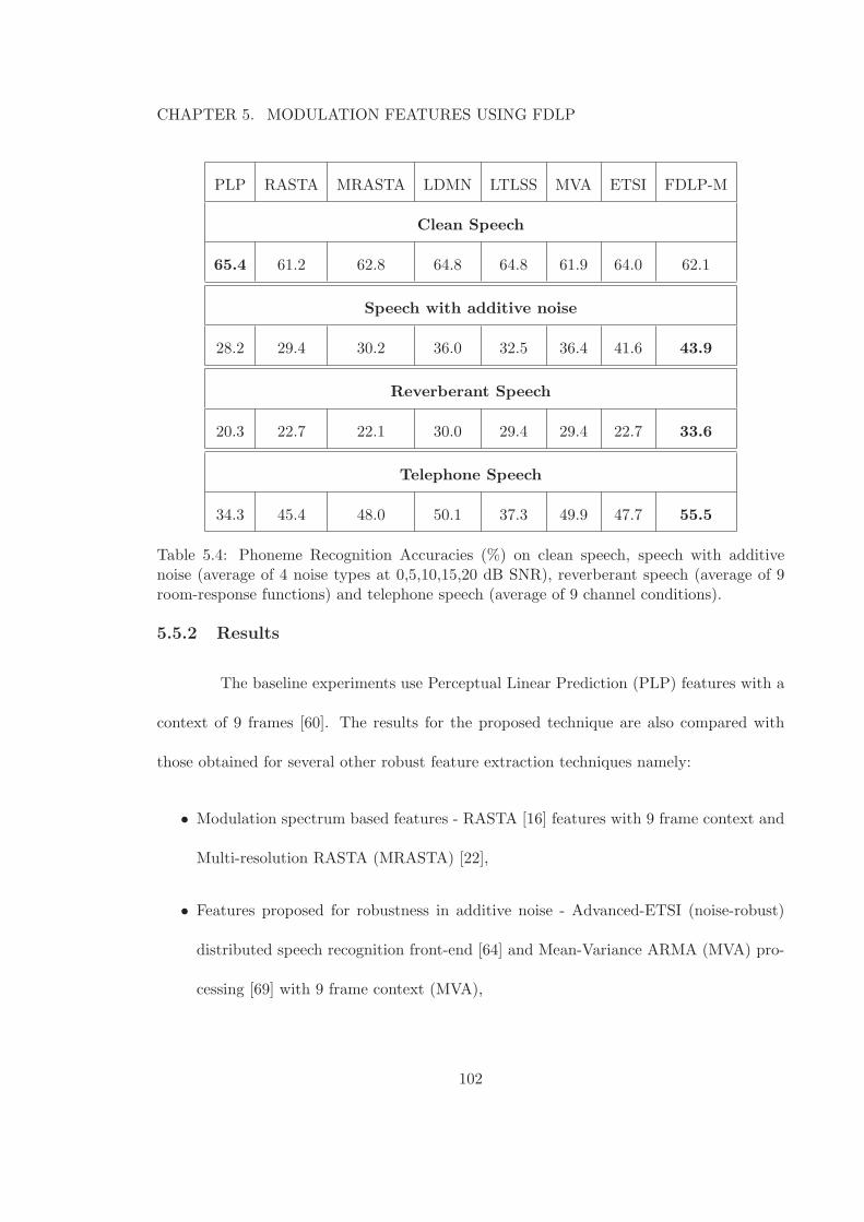
CHAPTER 5. MODULATION FEATURES USING FDLP
PLP RASTA MRASTA LDMN LTLSS MVA ETSI FDLP-M
Clean Speech
65.4 61.2 62.8 64.8 64.8 61.9 64.0 62.1
Speech with additive noise
28.2 29.4 30.2 36.0 32.5 36.4 41.6 43.9
Reverberant Speech
20.3 22.7 22.1 30.0 29.4 29.4 22.7 33.6
Telephone Speech
34.3 45.4 48.0 50.1 37.3 49.9 47.7 55.5
Table 5.4: Phoneme Recognition Accuracies (%) on clean speech, speech with additivenoise (average of 4 noise types at 0,5,10,15,20 dB SNR), reverberant speech (average of 9room-response functions) and telephone speech (average of 9 channel conditions).
5.5.2 Results
The baseline experiments use Perceptual Linear Prediction (PLP) features with a
context of 9 frames [60]. The results for the proposed technique are also compared with
those obtained for several other robust feature extraction techniques namely:
• Modulation spectrum based features - RASTA [16] features with 9 frame context and
Multi-resolution RASTA (MRASTA) [22],
• Features proposed for robustness in additive noise - Advanced-ETSI (noise-robust)
distributed speech recognition front-end [64] and Mean-Variance ARMA (MVA) pro-
cessing [69] with 9 frame context (MVA),
102
CHAPTER 5. MODULATION FEATURES USING FDLP
• Robust features for reverberant speech recognition - Long Term Log Spectral Sub-
traction (LTLSS) [41] and Log-DFT Mean Normalization (LDMN) [40] with 9 frame
context.
These techniques are chosen as baseline features as they are commonly deployed
in automatic speech and phoneme recognition systems. For the proposed FDLP based
modulation frequency features, we use 15 critical bands in the 300− 4000 Hz with an equal
band-width (in the bark frequency scale) of approx. 1 bark.
Table 5.4 shows the average phoneme recognition performance for the various
feature extraction techniques on clean speech, speech with additive noise, reverberant speech
and telephone channel speech. In clean conditions the baseline PLP feature extraction
technique provides the best performance. However, the performance of the PLP based
phoneme recognition system degrades significantly in all the mismatched conditions. In the
case of additive noise, the ETSI features give good robustness among the short-term spectral
features. For phoneme recognition in reverberant speech and telephone speech, LDMN and
MVA features provide good performance among the short-term spectral features.
In all the mismatched conditions, the FDLP features provide significant robustness
compared to other feature extraction techniques. On the average, the relative performance
improvement over the other feature extraction techniques is about 4 % for speech in additive
noise, 5 % for reverberant speech, and about 11 % for telephone speech.
The phoneme recognition performance on the individual noise types (“Restau-
rant”, “Babble”, “Subway” and “Exhibition Hall”) and SNR conditions (0-20 dB) is shown
in Table 5.4. Since the RASTA technique was mainly proposed for robustness in convolutive
103

CHAPTER 5. MODULATION FEATURES USING FDLP
SNR (dB) PLP GFCC MRASTA LDMN LTLSS MVA ETSI FDLP-M
Restaurant Noise
0 13.2 12.5 7.8 19.8 14.4 18.8 23.2 23.0
5 18.1 24.2 17.4 25.8 21.1 26.2 31.2 32.0
10 25.7 36.6 28.5 33.6 30.1 35.0 40.5 43.4
15 35.1 46.0 39.1 41.9 40.8 43.6 48.3 52.0
20 45.4 51.9 47.6 49.2 51.9 50.4 54.3 58.1
Babble Noise
0 12.2 10.5 6.0 18.8 13.9 16.1 20.8 22.4
5 16.3 21.9 15.2 24.2 19.6 25.1 29.5 31.3
10 23.4 34.7 26.5 31.8 28.2 34.4 39.0 43.2
15 32.7 45.6 37.6 40.8 39.2 43.1 47.9 53.0
20 43.8 52.2 47.5 49.2 51.3 50.3 54.6 58.7
Subway Noise
0 16.6 18.2 19.9 28.1 20.3 27.5 32.6 34.5
5 23.0 31.3 30.3 35.3 27.4 35.4 41.3 42.6
10 31.0 42.6 38.4 42.2 35.8 42.5 48.5 50.6
15 39.6 49.5 45.3 48.8 43.7 47.9 54.3 56.2
20 48.3 53.6 50.8 54.7 51.1 52.5 58.6 59.9
Exhibition Hall Noise
0 14.7 9.2 8.6 20.9 17.3 20.5 24.4 25.4
5 19.7 21.1 18.9 27.1 23.2 28.0 33.1 34.7
10 26.6 34.1 29.7 34.5 31.0 36.3 42.0 45.0
15 34.8 45.1 39.9 43.0 40.3 43.9 50.3 53.5
20 44.0 52.0 48.5 50.6 50.3 50.4 55.5 58.7
Table 5.5: Phoneme recognition accuracies (%) for 4 noise types at 0,5,10,15,20 dB SNRs.
104
CHAPTER 5. MODULATION FEATURES USING FDLP
distortions, we replace the RASTA features with the gammatone frequency cepstral coef-
ficients (GFCC [70]) for additive noise experiments reported in this table. These features
are auditory model based and the cepstral coefficients are derived directly from sub-band
energies (instead of log energies). The features are 29 dimensional and are appended with
first order derivatives [70]. We also apply a 9 frame context yielding GFCC features of
dimension 522.
In the experiments reported in Table 5.5, the ETSI technique [64] provides the best
baseline performance in all noise conditions. For almost all noise types and SNR conditions,
the proposed FDLP features provide good improvements over the best baseline features.
The improvements are significant for SNR values above 0 dB.
Although the proposed FDLP-M features provide good improvements on all con-
ditions of telephone, additive noise and reverberant speech (Table. 5.4), the contribution
of various stages to this performance improvement is unknown. In the next section, we
perform various phoneme recognition experiments to determine the importance of various
blocks in FDLP-M feature extraction.
5.6 Relative Contribution of Various Processing Stages
The previous section showed that the proposed feature extraction provides promis-
ing improvements in various types of distortions. In this section, we analyze the contribu-
tion of the various processing stages of the proposed feature extraction technique for robust
phoneme recognition. This is done by a set of phoneme recognition experiments on the
TIMIT database with various modifications of the proposed technique. As before, the sys-
105
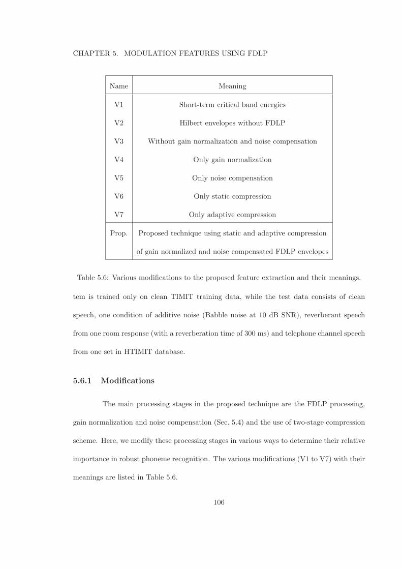
CHAPTER 5. MODULATION FEATURES USING FDLP
Name Meaning
V1 Short-term critical band energies
V2 Hilbert envelopes without FDLP
V3 Without gain normalization and noise compensation
V4 Only gain normalization
V5 Only noise compensation
V6 Only static compression
V7 Only adaptive compression
Prop. Proposed technique using static and adaptive compression
of gain normalized and noise compensated FDLP envelopes
Table 5.6: Various modifications to the proposed feature extraction and their meanings.
tem is trained only on clean TIMIT training data, while the test data consists of clean
speech, one condition of additive noise (Babble noise at 10 dB SNR), reverberant speech
from one room response (with a reverberation time of 300 ms) and telephone channel speech
from one set in HTIMIT database.
5.6.1 Modifications
The main processing stages in the proposed technique are the FDLP processing,
gain normalization and noise compensation (Sec. 5.4) and the use of two-stage compression
scheme. Here, we modify these processing stages in various ways to determine their relative
importance in robust phoneme recognition. The various modifications (V1 to V7) with their
meanings are listed in Table 5.6.
106
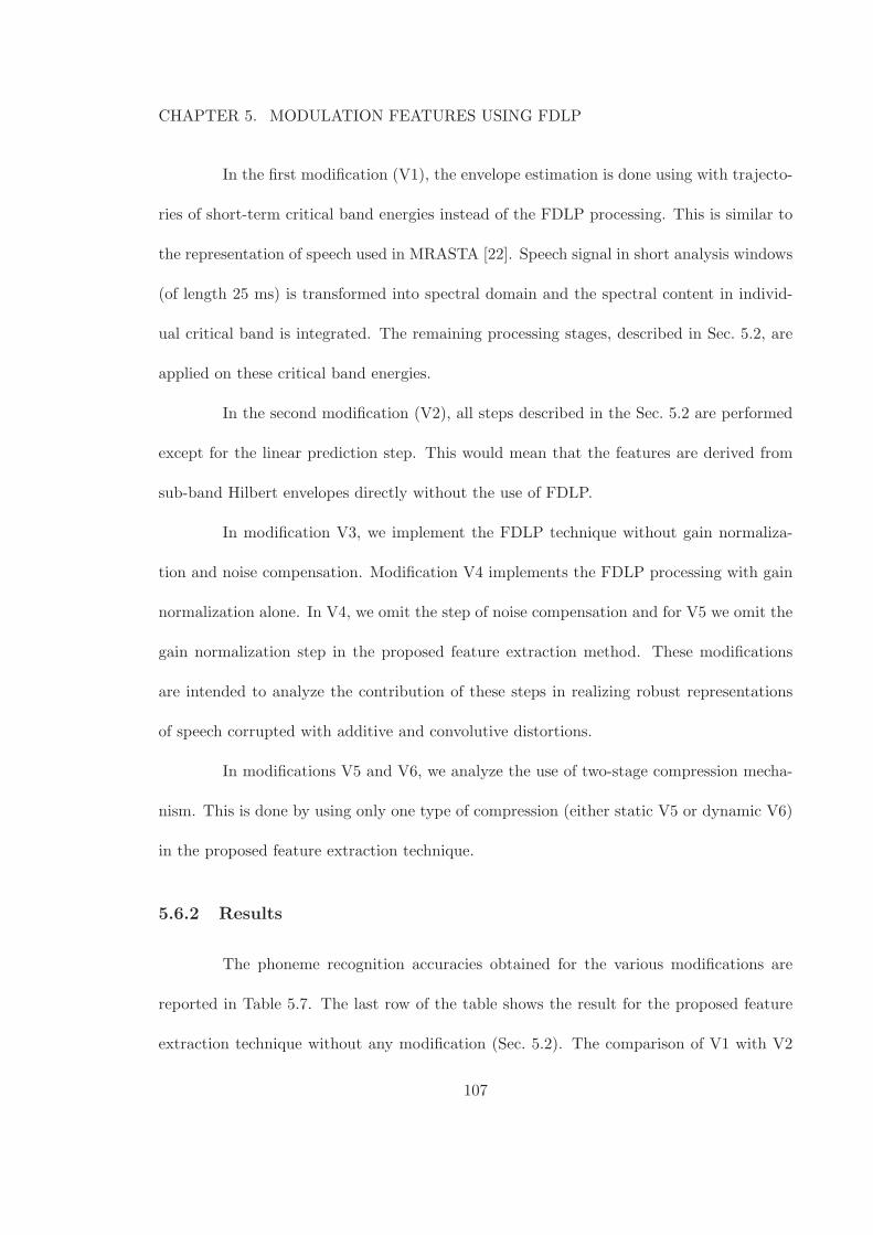
CHAPTER 5. MODULATION FEATURES USING FDLP
In the first modification (V1), the envelope estimation is done using with trajecto-
ries of short-term critical band energies instead of the FDLP processing. This is similar to
the representation of speech used in MRASTA [22]. Speech signal in short analysis windows
(of length 25 ms) is transformed into spectral domain and the spectral content in individ-
ual critical band is integrated. The remaining processing stages, described in Sec. 5.2, are
applied on these critical band energies.
In the second modification (V2), all steps described in the Sec. 5.2 are performed
except for the linear prediction step. This would mean that the features are derived from
sub-band Hilbert envelopes directly without the use of FDLP.
In modification V3, we implement the FDLP technique without gain normaliza-
tion and noise compensation. Modification V4 implements the FDLP processing with gain
normalization alone. In V4, we omit the step of noise compensation and for V5 we omit the
gain normalization step in the proposed feature extraction method. These modifications
are intended to analyze the contribution of these steps in realizing robust representations
of speech corrupted with additive and convolutive distortions.
In modifications V5 and V6, we analyze the use of two-stage compression mecha-
nism. This is done by using only one type of compression (either static V5 or dynamic V6)
in the proposed feature extraction technique.
5.6.2 Results
The phoneme recognition accuracies obtained for the various modifications are
reported in Table 5.7. The last row of the table shows the result for the proposed feature
extraction technique without any modification (Sec. 5.2). The comparison of V1 with V2
107
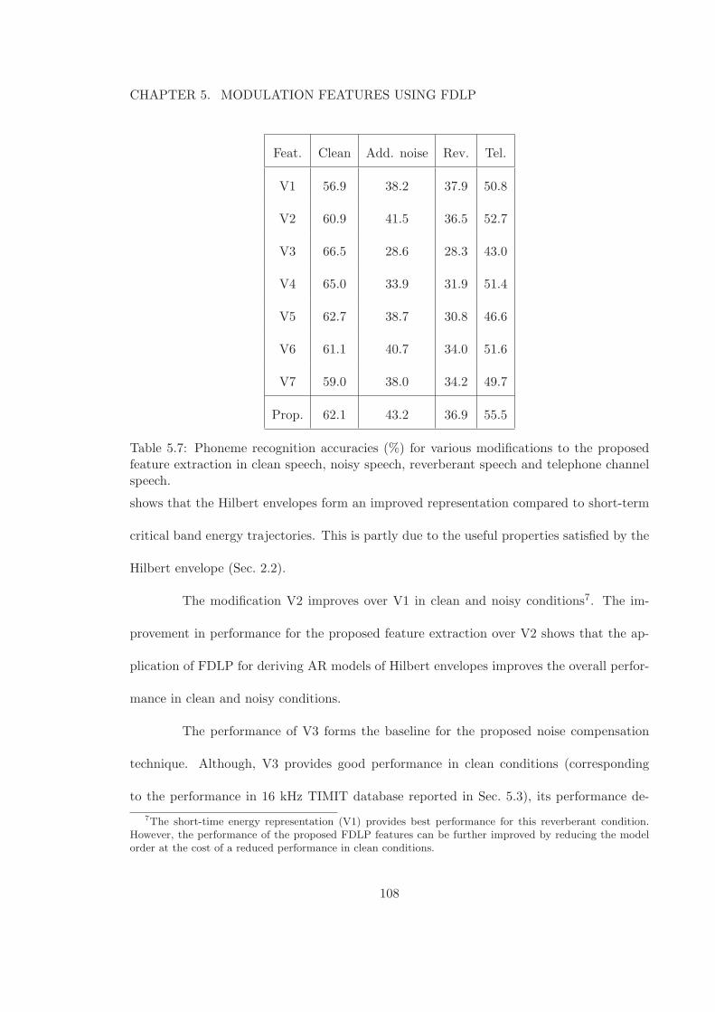
CHAPTER 5. MODULATION FEATURES USING FDLP
Feat. Clean Add. noise Rev. Tel.
V1 56.9 38.2 37.9 50.8
V2 60.9 41.5 36.5 52.7
V3 66.5 28.6 28.3 43.0
V4 65.0 33.9 31.9 51.4
V5 62.7 38.7 30.8 46.6
V6 61.1 40.7 34.0 51.6
V7 59.0 38.0 34.2 49.7
Prop. 62.1 43.2 36.9 55.5
Table 5.7: Phoneme recognition accuracies (%) for various modifications to the proposedfeature extraction in clean speech, noisy speech, reverberant speech and telephone channelspeech.
shows that the Hilbert envelopes form an improved representation compared to short-term
critical band energy trajectories. This is partly due to the useful properties satisfied by the
Hilbert envelope (Sec. 2.2).
The modification V2 improves over V1 in clean and noisy conditions7. The im-
provement in performance for the proposed feature extraction over V2 shows that the ap-
plication of FDLP for deriving AR models of Hilbert envelopes improves the overall perfor-
mance in clean and noisy conditions.
The performance of V3 forms the baseline for the proposed noise compensation
technique. Although, V3 provides good performance in clean conditions (corresponding
to the performance in 16 kHz TIMIT database reported in Sec. 5.3), its performance de-
7The short-time energy representation (V1) provides best performance for this reverberant condition.However, the performance of the proposed FDLP features can be further improved by reducing the modelorder at the cost of a reduced performance in clean conditions.
108
CHAPTER 5. MODULATION FEATURES USING FDLP
grades considerably in all noise conditions. The noise compensation technique provides
good robustness in additive noise conditions (V5). When this is applied along with the gain
normalization procedure, the resulting features (Prop.) improve significantly on all types of
distortions. The application of these techniques results in a drop in performance for clean
speech.
The reason for the reduction in performance in clean conditions maybe because
of the following reasons. The gain normalization of the sub-band envelope removes the
gain in each sub-band which can be a useful cue for phoneme recognition of clean speech
(as indicated by a moderate drop in performance in clean conditions for V3 and V4).
Furthermore, noise compensation technique tends to deemphasize the valleys of the envelope
trajectory. As the valleys of the envelope contain information in discriminating certain
phoneme classes (like nasals), there is a reduction in the recognition accuracy in clean
conditions (comparison of V3 and V5). However, the improvements obtained for all types
of mismatched conditions justify the employment of these normalization techniques in the
proposed features. The improvements are significant in telephone conditions (which can
be typically modeled a combined effect of short-term convolutive and additive distortions)
where the convolutive channel distortions are suppressed by the gain normalization and the
additive channel noise effects are reduced by the noise compensation block.
Finally, the application of log compression or adaptive compression alone is worse
than the joint application of these two compression schemes (V6-V7). Although this was
reported in Sec. 5.3.5 for clean conditions, we find here that the joint application of static
and dynamic compression schemes improved the performance in noisy conditions as well.
109
CHAPTER 5. MODULATION FEATURES USING FDLP
5.7 Chapter Summary
In this chapter, we have proposed the FDLP-M (FDLP modulation) features for
phoneme recognition in clean and noisy environment. We began with the discussion of the
modulation feature extraction scheme in Sec. 5.2. The performance of these features on
phoneme recognition experiments in matched conditions is reported in Sec. 5.3. In order to
improve the performance in mis-matched additive noise environments, we develop the noise
compensation technique for FDLP envelopes (Sec. 5.4). Note that, the noise compensation
technique is similar to the conventional spectral amplitude estimator [65] except for the
application of the technique in the sub-band analytic signal domain as opposed to complex
DFT domain.
The usefulness of the gain normalization and noise compensation techniques are
illustrated with phoneme recognition experiments in mis-matched conditions using speech
data corrupted with additive noise, reverberation and telephone channel distortions (Sec. 5.5).
In these experiments, the FDLP-M features provide significant improvements compared to
other noise robust front-ends.
The improvements provided by proposed features is attributed to various stages
in the feature extraction pipe-line. In order to determine the relative contributions of these
steps, we perform several phoneme recognition experiments using various modifications of
the proposed features (Sec. 5.6). The main findings from this analysis can be summarized
as follows:
• The application of linear prediction in frequency domain forms an efficient method
for deriving sub-band modulations.
110
CHAPTER 5. MODULATION FEATURES USING FDLP
• The two-stage compression scheme of deriving static and dynamic modulation spec-
trum results in good phoneme recognition for all phoneme classes even in the presence
of noise.
• The noise compensation technique provides a way to derive robust representation of
speech in almost all types of stationary noise and SNR conditions.
• The robustness of the proposed features is further enhanced by the application of gain
normalization technique.
• The noise compensation techniques provide substantial improvements in additive noise
conditions and performs well in combination with the gain-normalization scheme in
reverberant and telephone channel conditions.
In the next chapter, we investigate the application of FDLP representation for audio coding.
111
Chapter 6
FDLP based Audio Coding
6.1 Chapter Outline
Recently, there has been many initiatives in standardization organizations like 3GPP, ITU-
T, and MPEG (for example [71]) that aim for the development of a unified codec which can
efficiently compress all kinds of speech and audio signals and which may require new audio
compression techniques. In traditional applications of speech coding (i.e., for conversational
services), the algorithmic delay of the codec is one of the most critical variables. However,
there are many services, such as audio file downloads, voice messaging etc., where the issue
of the codec delay is much less critical. This allows for a whole set of different analysis
and compression techniques that could be more effective than the conventional short-term
frame based coding techniques.
In this chapter, we present a scalable medium bit-rate wide-band audio coding
for signal sampled at 48 kHz. The encoding technique based on frequency domain linear
prediction (FDLP). The main goal of the proposed audio codec is to illustrate the use of
112
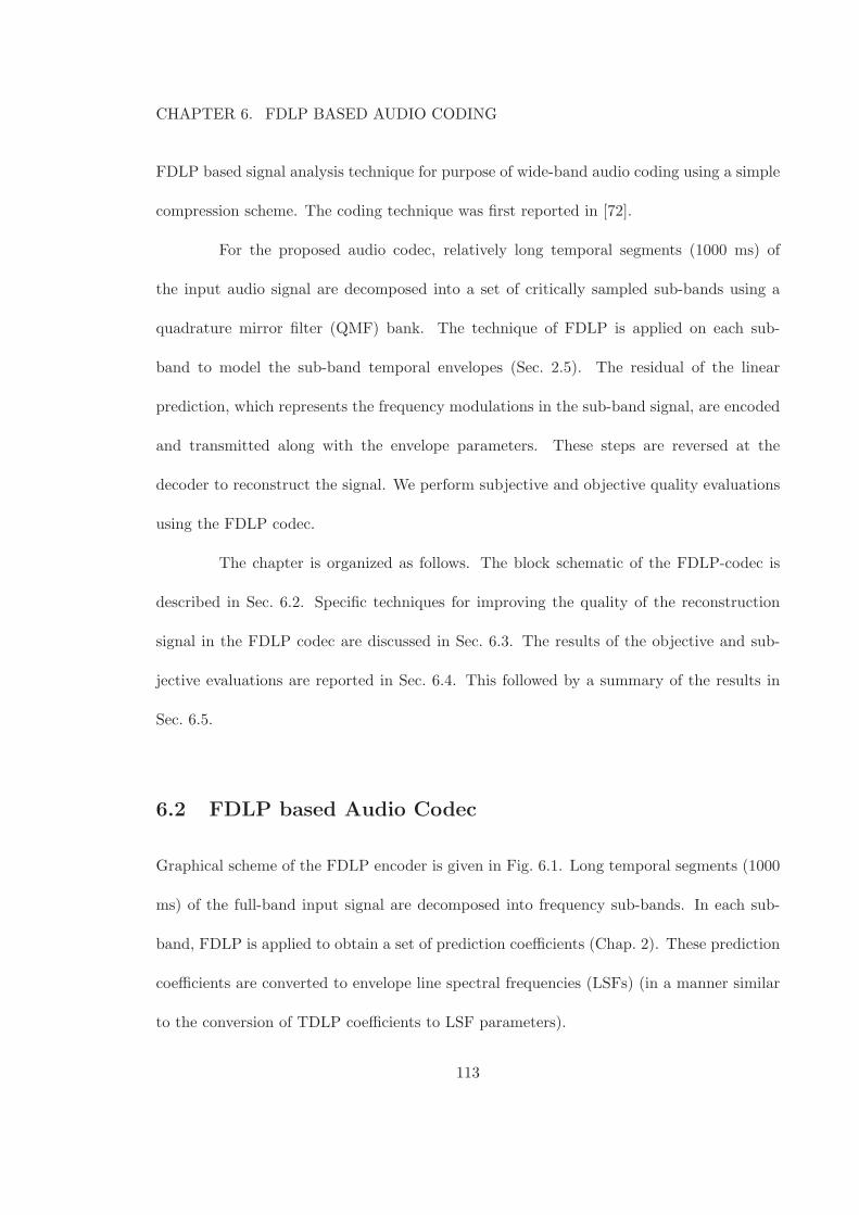
CHAPTER 6. FDLP BASED AUDIO CODING
FDLP based signal analysis technique for purpose of wide-band audio coding using a simple
compression scheme. The coding technique was first reported in [72].
For the proposed audio codec, relatively long temporal segments (1000 ms) of
the input audio signal are decomposed into a set of critically sampled sub-bands using a
quadrature mirror filter (QMF) bank. The technique of FDLP is applied on each sub-
band to model the sub-band temporal envelopes (Sec. 2.5). The residual of the linear
prediction, which represents the frequency modulations in the sub-band signal, are encoded
and transmitted along with the envelope parameters. These steps are reversed at the
decoder to reconstruct the signal. We perform subjective and objective quality evaluations
using the FDLP codec.
The chapter is organized as follows. The block schematic of the FDLP-codec is
described in Sec. 6.2. Specific techniques for improving the quality of the reconstruction
signal in the FDLP codec are discussed in Sec. 6.3. The results of the objective and sub-
jective evaluations are reported in Sec. 6.4. This followed by a summary of the results in
Sec. 6.5.
6.2 FDLP based Audio Codec
Graphical scheme of the FDLP encoder is given in Fig. 6.1. Long temporal segments (1000
ms) of the full-band input signal are decomposed into frequency sub-bands. In each sub-
band, FDLP is applied to obtain a set of prediction coefficients (Chap. 2). These prediction
coefficients are converted to envelope line spectral frequencies (LSFs) (in a manner similar
to the conversion of TDLP coefficients to LSF parameters).
113
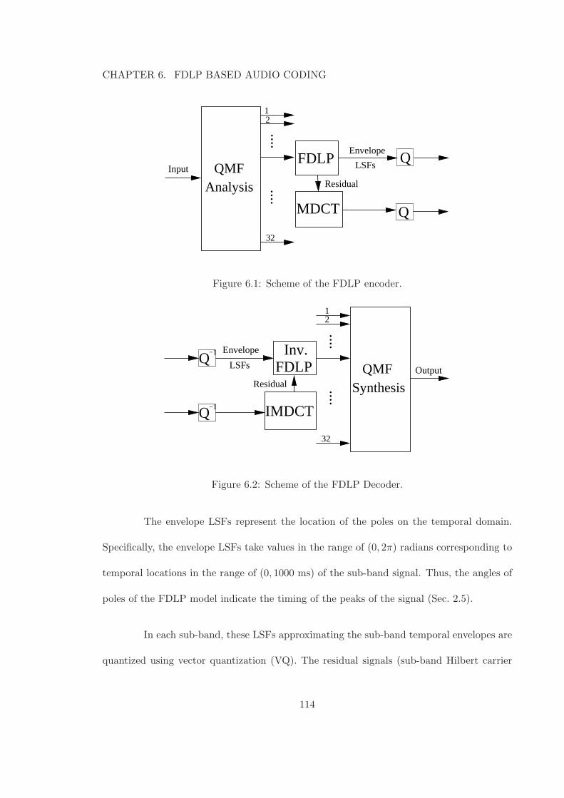
CHAPTER 6. FDLP BASED AUDIO CODING
....
32
21
InputFDLP
Residual
EnvelopeQ
....
QMFAnalysis
LSFs
QMDCT
Figure 6.1: Scheme of the FDLP encoder.
Q−1
Q−1
QMF
32
21
Output
........Inv.
FDLPEnvelope
LSFs
SynthesisResidual
IMDCT
Figure 6.2: Scheme of the FDLP Decoder.
The envelope LSFs represent the location of the poles on the temporal domain.
Specifically, the envelope LSFs take values in the range of (0, 2π) radians corresponding to
temporal locations in the range of (0, 1000 ms) of the sub-band signal. Thus, the angles of
poles of the FDLP model indicate the timing of the peaks of the signal (Sec. 2.5).
In each sub-band, these LSFs approximating the sub-band temporal envelopes are
quantized using vector quantization (VQ). The residual signals (sub-band Hilbert carrier
114
CHAPTER 6. FDLP BASED AUDIO CODING
signals) are processed in transform domain using the modified discrete cosine transform
(MDCT). The MDCT coefficients are also quantized using VQ.
In the decoder, shown in Fig. 6.2, quantized MDCT coefficients of the FDLP
residual signals are reconstructed and transformed back to the time-domain using inverse
MDCT (IMDCT). The reconstructed FDLP envelopes (obtained from LSF parameters) are
used to modulate the corresponding sub-band residual signals. Finally, sub-band synthesis
is applied to reconstruct the full-band signal.
The important blocks are:
6.2.1 Non-uniform sub-band decomposition
A non-uniform quadrature mirror filter (QMF) bank is used for the sub-band decomposi-
tion of the input audio signal. QMF provides sub-band sequences which form a critically
sampled and maximally decimated signal representation (i.e., the total number of sub-band
samples is equal to the number of input samples). In the proposed non-uniform QMF
analysis, the input audio signal (sampled at 48 kHz) is split into 1000 ms long frames.
Each frame is decomposed using a 6 stage tree-structured uniform QMF analysis to pro-
vide 64 uniformly spaced sub-bands. A non-uniform QMF decomposition into 32 frequency
sub-bands is obtained by merging these 64 uniform QMF sub-bands [73]. This sub-band
decomposition is motivated by critical band decomposition in the human auditory system.
Many uniformly spaced sub-bands at the higher auditory frequencies are merged together
while maintaining perfect reconstruction. The non-uniform QMF decomposition provides a
good compromise between fine spectral resolution for low frequency sub-bands and a smaller
number of encoding bits for higher bands.
115
CHAPTER 6. FDLP BASED AUDIO CODING
In order to reduce the leakage of quantization noise from one sub-band to another,
the QMF analysis and synthesis filters are desired to have a sharp transition band. However,
this would result in a significant delay for the QMF filter bank. Since we use an initial
decomposition using a tree structured QMF filter bank, the overall filter bank delay can be
considerably reduced by reducing the length of filters in the successive stages of the tree.
Although the width of the transition band in the sub-sampled domain increases due to the
reduction in filter length, the transition bandwidth at the original sampling rate remains
the same [74]. The overall delay for the proposed QMF filter bank is about 30 ms.
6.2.2 Encoding FDLP residual signals using MDCT
We propose an encoding scheme for the FDLP residual signals using MDCT. The MDCT,
originally proposed in [75], outputs a set of critically sampled transform domain coefficients.
Perfect reconstruction is provided by time domain alias cancellation and the overlapped
nature of the transform.
For the proposed FDLP codec, the sub-band FDLP residual signals are split into
relatively short frames (50 ms) and transformed using the MDCT. We use the sine window
with 50% overlap for the MDCT analysis as this was experimentally found to provide the
best reconstruction quality (based on objective quality evaluations). Since a full-search VQ
in the MDCT domain with good resolution would be computationally infeasible, the split
VQ approach is employed. Although the split VQ approach is suboptimal, it reduces the
computational complexity and memory requirements to manageable limits without severely
degrading the VQ performance. The quantized levels are Huffman encoded for further
reduction of bit-rates. This entropy coding scheme results in a bit-rate reduction of about
116
CHAPTER 6. FDLP BASED AUDIO CODING
10%. The MDCT coefficients for the lower frequency sub-bands are quantized using higher
number of VQ levels as compared to those from the higher bands. VQ of the MDCT
coefficients from the FDLP carrier signal consumes about 80% of the final bit-rate.
For the purpose of scaling the bit-rates, all sub-bands are treated uniformly and
the number of VQ levels are suitably modified so as to meet the specified bit-rate. The
current version of the codec follows a simple bit assignment mechanism for the MDCT
coefficients and provides bit-rate scalability in the range of 32-64 kbps.
6.3 Techniques for Quality Enhancement
In this section, we discuss two techniques used in FDLP codec for improving the reconstruc-
tion quality of the audio signal. These techniques are temporal masking [76] and spectral
noise shaping [77].
6.3.1 Temporal Masking
The auditory masking properties of the human ear provide an efficient solution for quan-
tization of a signal in such a way that the audible distortion is minimized. In particular,
temporal masking is a property of the human ear, where the sounds appearing within a
temporal interval of about 200 ms after a signal component get masked.
The long term processing (1000 ms) in the FDLP codec allows for a straightforward
exploitation of the temporal masking, while its implementation in more conventional short-
term spectra based codecs has been so far quite limited.
Temporal masking can be explained as a change in the time course of recovery
117
CHAPTER 6. FDLP BASED AUDIO CODING
from masking [78]. The amount of forward masking is determined by the interaction of a
number of factors including masker level, the temporal separation of the masker and the
signal, frequency of the masker and the signal and duration of the masker and the signal [78].
A simple first order mathematical model, which provides a sufficient approximation for the
amount of temporal masking, is given as
M [n] = a(b− log10∆t)(X[n]− c), (6.1)
where M is the temporal mask in dB Sound Pressure Level (SPL), X is the signal dB SPL
level, n is the sample index, ∆t is the time delay in ms, a, b and c are the constants. At
any sample point, multiple mask estimates arising from the several previous samples are
present and the maximum value is chosen as the mask in dB SPL. The optimal values of
these parameters, as defined in [79], are as follows:
a = k2f2 + k1f + k0, (6.2)
where f is the center frequency of the sub-band in kHz, k0, k1 and k2 are constants. The
constant b denotes the duration of the temporal masking and is chosen as log10 200. The
parameter c is the Absolute Threshold of Hearing (ATH) in quiet, defined as:
c = 3.64f−0.8 − 6.5e−0.6(f−3.3)2 + 0.001f4. (6.3)
An alternative SPL definition
A short-term SPL definition is needed to estimate the masking threshold at each sample
index. For this purpose, the signal is divided into 10 ms overlapping frames with frame
shifts of 1 sample. The estimated short term power in SPL is assigned to the middle sample
118
CHAPTER 6. FDLP BASED AUDIO CODING
of the frame:
X[n] = 10 log10
[
∑n+L2
i=n−L2
x2[i]
L
]
, (6.4)
where X is the signal in dB SPL, x denotes the original time domain signal and L denotes
the frame length (10 ms).
In our FDLP codec, the linear forward masking model proposed in [78] is applied to
the QMF sub-band signal. The masking thresholds are determined on the sub-band signal.
These masking thresholds are then utilized in quantizing the sub-band FDLP carrier signals.
Application of the temporal mask for encoding the sub-band FDLP carriers
The number of bits required for representing the sub-band FDLP carrier is reduced in
accordance with the temporal masking thresholds. Since the sub-band signal is the product
of its FDLP envelope and carrier, the masking thresholds for the carrier signal are obtained
by subtracting the dB SPL of the envelope from that of the sub-band signal.
The first step is to estimate the quantization noise present in the base-line version;
if the mean of the quantization noise (in 200 ms sub-band signal) is above the masking
threshold, no bit-rate reduction is applied. If the temporal mask mean is above the noise
mean, then the amount of bits needed to encode that sub-band carrier signal is reduced in
such a way that the noise level becomes similar to the masking threshold. This is illustrated
in Fig. 6.3, where we plot the level of quantization noise in the baseline codec (without
temporal masking), the masking threshold level, and the level of quantization noise after
bit-rate reduction in order to match the masking threshold. A reduction in bit-rate without
loss in quality transpires to improvements in the reconstruction quality at the same bit-rate.
119
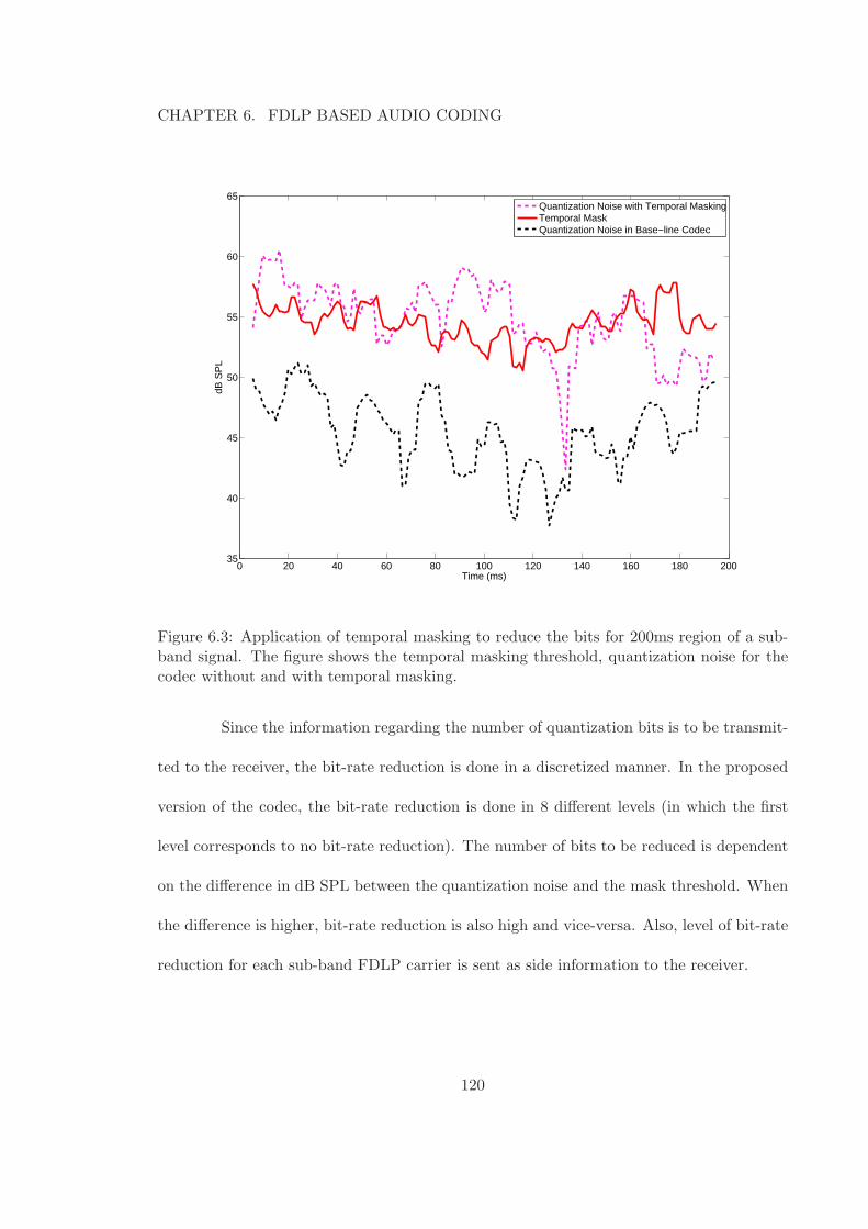
CHAPTER 6. FDLP BASED AUDIO CODING
0 20 40 60 80 100 120 140 160 180 20035
40
45
50
55
60
65
Time (ms)
dB S
PL
Quantization Noise with Temporal MaskingTemporal MaskQuantization Noise in Base−line Codec
Figure 6.3: Application of temporal masking to reduce the bits for 200ms region of a sub-band signal. The figure shows the temporal masking threshold, quantization noise for thecodec without and with temporal masking.
Since the information regarding the number of quantization bits is to be transmit-
ted to the receiver, the bit-rate reduction is done in a discretized manner. In the proposed
version of the codec, the bit-rate reduction is done in 8 different levels (in which the first
level corresponds to no bit-rate reduction). The number of bits to be reduced is dependent
on the difference in dB SPL between the quantization noise and the mask threshold. When
the difference is higher, bit-rate reduction is also high and vice-versa. Also, level of bit-rate
reduction for each sub-band FDLP carrier is sent as side information to the receiver.
120
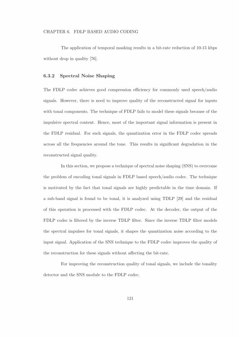
CHAPTER 6. FDLP BASED AUDIO CODING
The application of temporal masking results in a bit-rate reduction of 10-15 kbps
without drop in quality [76].
6.3.2 Spectral Noise Shaping
The FDLP codec achieves good compression efficiency for commonly used speech/audio
signals. However, there is need to improve quality of the reconstructed signal for inputs
with tonal components. The technique of FDLP fails to model these signals because of the
impulsive spectral content. Hence, most of the important signal information is present in
the FDLP residual. For such signals, the quantization error in the FDLP codec spreads
across all the frequencies around the tone. This results in significant degradation in the
reconstructed signal quality.
In this section, we propose a technique of spectral noise shaping (SNS) to overcome
the problem of encoding tonal signals in FDLP based speech/audio codec. The technique
is motivated by the fact that tonal signals are highly predictable in the time domain. If
a sub-band signal is found to be tonal, it is analyzed using TDLP [29] and the residual
of this operation is processed with the FDLP codec. At the decoder, the output of the
FDLP codec is filtered by the inverse TDLP filter. Since the inverse TDLP filter models
the spectral impulses for tonal signals, it shapes the quantization noise according to the
input signal. Application of the SNS technique to the FDLP codec improves the quality of
the reconstruction for these signals without affecting the bit-rate.
For improving the reconstruction quality of tonal signals, we include the tonality
detector and the SNS module to the FDLP codec.
121

CHAPTER 6. FDLP BASED AUDIO CODING
SNS
Encoder
Sub−band
Reconstructed
Sub−band
Filtering
No
Tonality Detector
Sub−band
Inverse TDLPYes TDLPFiltering
QMF FDLPAnalysis
FDLPSynthesis
Decoder
FDLPAnalysis
FDLPSynthesis
Reconstructed
Figure 6.4: Sub-band processing in FDLP codec with SNS.
Implementation of SNS
Fig. 6.4 shows the block schematic of the FDLP codec with SNS. The only ad-
ditional side information is the signaling of the tonality decision to the decoder (32bps).
The tonal sub-band signals are applied to a TDLP filtering block. For the tonal signals,
the TDLP and the FDLP model order are made equal to half the FDLP model order used
for the non-tonal signals. Hence, there is no increase in the bit-rate by the inclusion of the
SNS (except for the signaling of the tonality flag) as the number of LP coefficients to be
quantized remains the same. At the decoder, inverse TDLP filtering applied on the FDLP
decoded signal gives the sub-band signal back.
The technique of SNS is motivated by the fundamental property of the linear pre-
diction: For AR signals, the inverse TDLP filter has magnitude response characteristics
similar to the Power Spectral Density (PSD) of the input signal [29]. Since the quantiza-
tion noise passes through the inverse TDLP filter, it gets shaped in the frequency domain
122
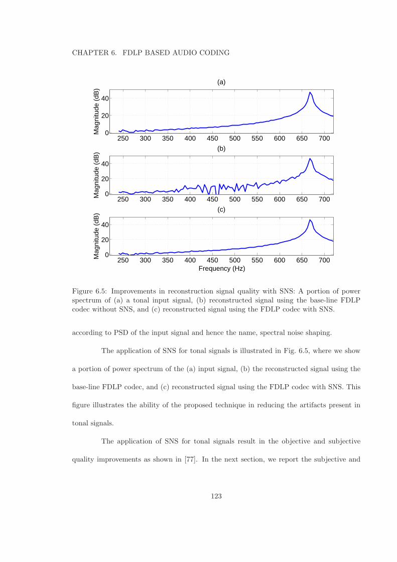
CHAPTER 6. FDLP BASED AUDIO CODING
250 300 350 400 450 500 550 600 650 7000
20
40M
agni
tude
(dB
)
(a)
250 300 350 400 450 500 550 600 650 7000
20
40
(b)
Mag
nitu
de (
dB)
250 300 350 400 450 500 550 600 650 7000
20
40
(c)
Frequency (Hz)
Mag
nitu
de (
dB)
Figure 6.5: Improvements in reconstruction signal quality with SNS: A portion of powerspectrum of (a) a tonal input signal, (b) reconstructed signal using the base-line FDLPcodec without SNS, and (c) reconstructed signal using the FDLP codec with SNS.
according to PSD of the input signal and hence the name, spectral noise shaping.
The application of SNS for tonal signals is illustrated in Fig. 6.5, where we show
a portion of power spectrum of the (a) input signal, (b) the reconstructed signal using the
base-line FDLP codec, and (c) reconstructed signal using the FDLP codec with SNS. This
figure illustrates the ability of the proposed technique in reducing the artifacts present in
tonal signals.
The application of SNS for tonal signals result in the objective and subjective
quality improvements as shown in [77]. In the next section, we report the subjective and
123
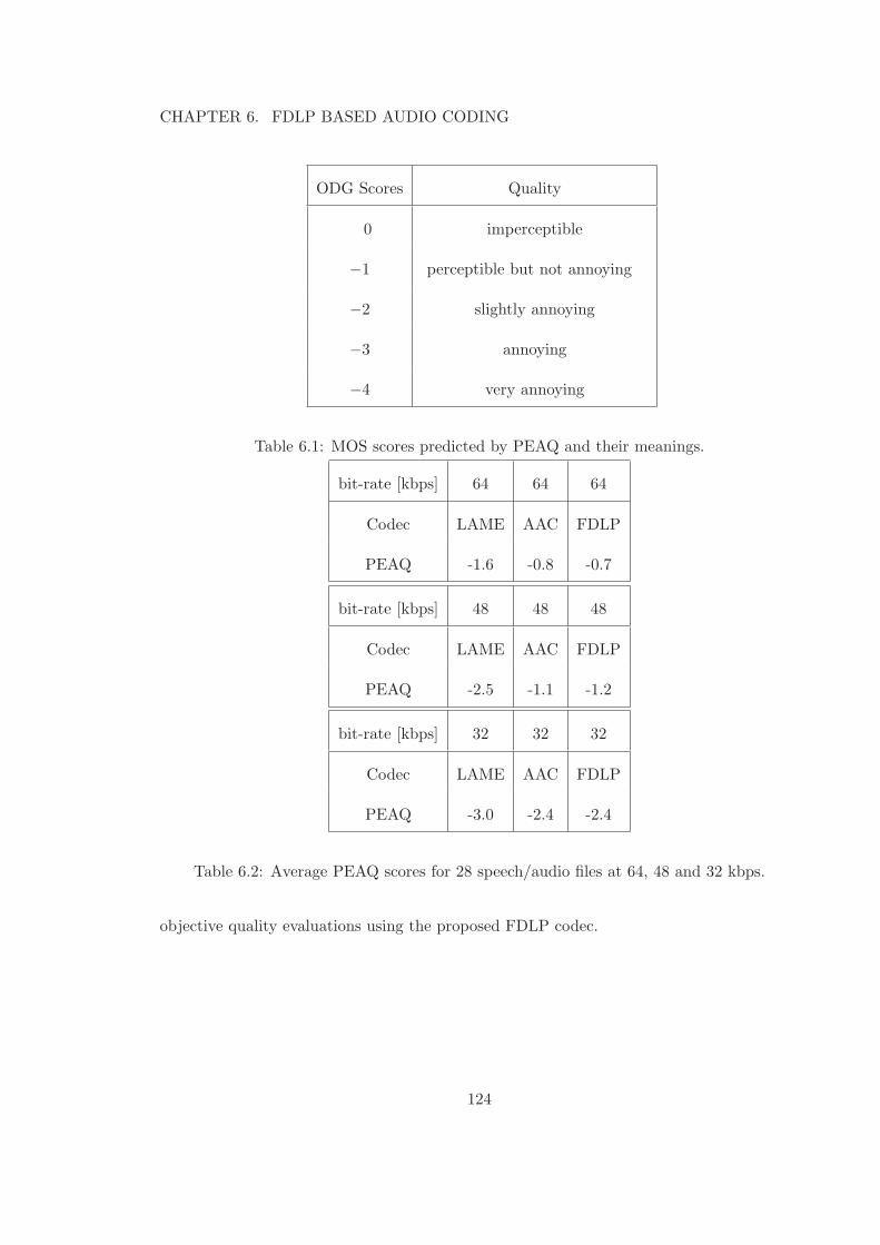
CHAPTER 6. FDLP BASED AUDIO CODING
ODG Scores Quality
0 imperceptible
−1 perceptible but not annoying
−2 slightly annoying
−3 annoying
−4 very annoying
Table 6.1: MOS scores predicted by PEAQ and their meanings.
bit-rate [kbps] 64 64 64
Codec LAME AAC FDLP
PEAQ -1.6 -0.8 -0.7
bit-rate [kbps] 48 48 48
Codec LAME AAC FDLP
PEAQ -2.5 -1.1 -1.2
bit-rate [kbps] 32 32 32
Codec LAME AAC FDLP
PEAQ -3.0 -2.4 -2.4
Table 6.2: Average PEAQ scores for 28 speech/audio files at 64, 48 and 32 kbps.
objective quality evaluations using the proposed FDLP codec.
124

CHAPTER 6. FDLP BASED AUDIO CODING
6.4 Quality Evaluations
The subjective and objective evaluations of the proposed audio codec are per-
formed using audio signals (sampled at 48 kHz) present in the framework for exploration of
speech and audio coding [71, 80]. This database is comprised of speech, music and speech
over music recordings. The music samples contain a wide variety of challenging audio
samples ranging from tonal signals to highly transient signals.
The objective and subjective quality evaluations of the following codecs are con-
sidered:
1. The proposed FDLP codec with MDCT based residual signal processing, at 32, 48
and 64 kbps, denoted as FDLP.
2. LAME MP3 (MPEG 1, layer 3)1, at 32, 48 and 64, kbps denoted as LAME.
3. MPEG-4 HE-AAC, v1, at 32, 48 and 64 kbps [81], denoted as AAC. The HE-AAC
coder is the combination of spectral band replication (SBR) [82] and advanced audio
coding (AAC) [3].
6.4.1 Objective Evaluations
The objective measure employed is the perceptual evaluation of audio quality
(PEAQ) distortion measure [83]. In general, the perceptual degradation of the test signal
with respect to the reference signal is measured, based on the ITU-R BS.1387 (PEAQ)
standard. The output combines a number of model output variables (MOV’s) into a single
measure, the objective difference grade (ODG) score, which is an impairment scale with
1LAME-MP3 codec: http://lame.sourceforge.net
125
CHAPTER 6. FDLP BASED AUDIO CODING
meanings shown in Tab. 6.1. The mean PEAQ score for the 28 speech/audio files from [80]
is used as the objective quality measure.
The results in Tab. 6.2 also show the average PEAQ scores for the proposed FDLP
codec, AAC and LAME codecs at 64, 48 and 32 kbps. The objective scores for the proposed
FDLP codec at these bit-rates are better than MP3 codec and compares well with the state-
of-art AAC codec.
6.4.2 Subjective Evaluations
In this section, we report the results of subjective evaluations using the FDLP
codec. We report the performance only at 48 kbps. The other results at 64 and 32 kbps
can be found in [72].
For the audio signals encoded at 48 kbps, the MUSHRA (MUltiple Stimuli with
Hidden Reference and Anchor) methodology for subjective evaluation is employed. It is
defined by ITU-R recommendation BS.1534 [84]. We perform the MUSHRA tests on 6
speech/audio samples from the database. The mean MUSHRA scores (with 95% confidence
interval), for the subjective listening tests at 48 kbps (given in Fig. 6.6), show that the
subjective quality of the proposed codec is slightly poorer compared to the AAC codec
but better than the LAME codec. Here, the results are split into individual sample types
(namely speech, mixed and music content). The subjective scores for FDLP codec are
higher for the audio samples with music and mixed content compared to those with speech
content.
126
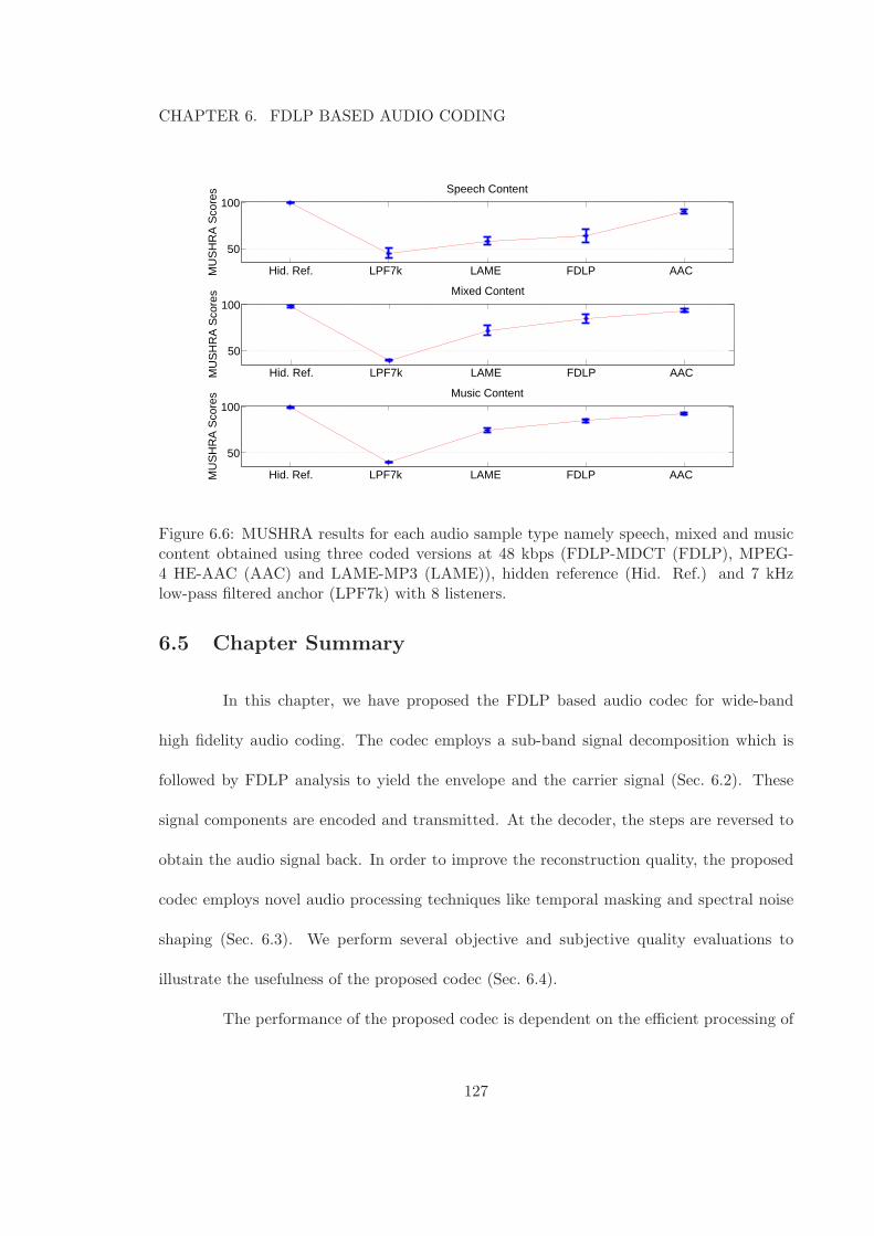
CHAPTER 6. FDLP BASED AUDIO CODING
Hid. Ref. LPF7k LAME FDLP AAC
50
100
MU
SH
RA
Sco
res Music Content
Hid. Ref. LPF7k LAME FDLP AAC
50
100
MU
SH
RA
Sco
res Mixed Content
Hid. Ref. LPF7k LAME FDLP AAC
50
100M
US
HR
A S
core
s Speech Content
Figure 6.6: MUSHRA results for each audio sample type namely speech, mixed and musiccontent obtained using three coded versions at 48 kbps (FDLP-MDCT (FDLP), MPEG-4 HE-AAC (AAC) and LAME-MP3 (LAME)), hidden reference (Hid. Ref.) and 7 kHzlow-pass filtered anchor (LPF7k) with 8 listeners.
6.5 Chapter Summary
In this chapter, we have proposed the FDLP based audio codec for wide-band
high fidelity audio coding. The codec employs a sub-band signal decomposition which is
followed by FDLP analysis to yield the envelope and the carrier signal (Sec. 6.2). These
signal components are encoded and transmitted. At the decoder, the steps are reversed to
obtain the audio signal back. In order to improve the reconstruction quality, the proposed
codec employs novel audio processing techniques like temporal masking and spectral noise
shaping (Sec. 6.3). We perform several objective and subjective quality evaluations to
illustrate the usefulness of the proposed codec (Sec. 6.4).
The performance of the proposed codec is dependent on the efficient processing of
127
CHAPTER 6. FDLP BASED AUDIO CODING
the FDLP carrier signal. It is important to note that the FDLP codec does not use standard
blocks like simultaneous masking which are widely used in standard codecs [3]. Inclusion of
some of these sophisticated bit-rate reduction techniques should further reduce the target
bit-rates and enhance the bit-rate scalability.
The present chapter along with the Chap. 4 and Chap. 5 has shown that FDLP
based signal analysis can be used for various signal applications like speech recognition,
modulation feature extraction and coding. In the next chapter, we show discuss future
extensions of the proposed methodologies.
128
Chapter 7
Summary and Future Extensions
7.1 Chapter Outline
In this chapter, we summarize the important contributions from this thesis. We highlight
different properties of the FDLP model which make it useful in various applications. We
also discuss the limitations of the FDLP model and the scope of applicability. The chapter
ends with a brief outline of various extensions of this thesis.
Sec. 7.2 highlight the main contributions of the thesis. Sec. 7.3 discusses the
limitations and scope of the thesis in speech signal processing. Finally, we discuss various
extensions of the FDLP technique in Sec. 7.4. We conclude the chapter in Sec. 7.5
7.2 Contributions of the Thesis
In this thesis, we have proposed the use of long-term AM-FM modeling for representing
speech/audio signals. This approach is fundamentally different from the conventional short-
129
CHAPTER 7. SUMMARY AND FUTURE EXTENSIONS
term spectrum based analysis. Specifically, we have developed an AR model of sub-band
Hilbert envelope and derived two-dimensional time-frequency representation of signals using
these models.
The thesis also developed various techniques for robust representation of speech
signals in noisy and reverberant environments. These techniques were applied along with
FDLP model for developing feature extraction methodologies. We use these representation
to develop two types of acoustic features - the short-term features (FDLP-S) which are
similar to conventional MFCCs and the long-term high dimensional modulation features
(FDLP-M). By efficient encoding of FDLP carrier signal, we also apply the FDLP analysis
for audio coding task.
The novel contributions from this thesis can be summarized as -
1. A simple mathematical proof for the AR model of Hilbert envelopes (Chap. 2,
Sec. 2.5) - The main difference between our derivation and those present in [27] is
that the proposed method uses a algebraic and verbal method for arguments in the
derivation and makes mild assumptions (of zero mean property in time and frequency
domain) to simplify the analysis. The underlying steps involved are a simplistic ver-
sion of the matrix derivation [27]. The proof provided in [26] uses analog signal
notations. Here, we use basic Fourier transform relations and discrete time analytic
signal representations.
2. Understanding the resolving power of AR modeling (Chap. 2, Sec. 2.6) -
To the best of our knowledge, the investigation of resolution properties of AR models
has not been done in the past. We define a measure of resolving power as the critical
130
CHAPTER 7. SUMMARY AND FUTURE EXTENSIONS
duration below which two peaks in the input merge together at the output of the AR
model. Then, we experiment with signals having two distinct peaks whose locations
are varied to determine the critical duration. This analysis shows that the critical
duration (resolution) is dependent on the starting location of the peak. Higher resolu-
tion (lower critical duration) is obtained at the center of the window. The resolution
is also dependent the type of window used and model order. One possible solution
to improve the resolution at the boundaries of the window is by padding the signal
(even-symmetrically).
3. Gain normalization of FDLP envelopes (Chap. 3, Sec. 3.5) - The effect of
convolutive artifacts like room reverberation on the FDLP envelope can be analyzed.
With a first-order approximation and the use of a long-term narrow-band analysis,
we have shown that the effect of reverberation can be suppressed by normalizing the
gain of the sub-band FDLP model. The gain normalization reduces the mis-match
between the envelopes extracted from clean and reverberant speech.
4. Short-term feature extraction for speech and speaker recognition (Chap. 4
) - Short-term feature extraction is obtained by integrating the FDLP spectrogram in
short-term windows. The envelopes are derived from gain normalized FDLP model.
These features are similar to conventional MFCC features. In speech recognition, the
gain normalization for FDLP-S features provides significant improvements in rever-
berant and telephone channel conditions. Furthermore, the trade-off in the choice of
various parameters like type of window, FDLP model order, envelope expansion factor
and the nature of sub-band analysis have been investigated along with their influence
131
CHAPTER 7. SUMMARY AND FUTURE EXTENSIONS
on the final ASR performance.
5. Modulation feature extraction for phoneme recognition (Chap. 5 ) - We
propose a modulation feature extraction scheme using FDLP spectrogram. We use a
two-stage processing with static and dynamic compression. The compressed envelopes
are converted into modulation features in syllable length segments. We also derive a
noise compensation scheme for temporal envelope estimation in additive noise condi-
tions. Various phoneme recognition experiments are done to illustrate the usefulness
of these representations as well as to investigate the contribution of various modules
in the feature computation.
6. Audio coding using FDLP (Chap. 6 ) - We propose a wide-band high fidelity
audio coding technique using FDLP based analysis in each QMF sub-band. Efficient
encoding scheme is developed using the application of novel techniques like temporal
masking and spectral noise shaping.
In the next section, we outline the various assumptions and limitations used in the FDLP
model and the scope of applicability of FDLP based analysis in speech/audio systems.
7.3 Limitations of FDLP analysis
The FDLP model was proposed as an unified signal analysis technique using the sub-band
AM-FM decomposition. This model has some fundamental limitations and assumptions
which are detailed in this section.
132
CHAPTER 7. SUMMARY AND FUTURE EXTENSIONS
• Limitations in AR modeling - The major assumption in the FDLP model is that
the envelope can be approximated using an all-pole model. When the envelope has
zeros, or when the envelope is constant over the entire analysis window, the FDLP
representation is unable to approximate the envelope. A simple example is that a
sinusoid cannot be well represented using the FDLP model. One possibility to model
such a sinusoid is the use of a TDLP model before the FDLP (spectral noise shaping,
Sec. 6.3.2).
• Convolution model in gain normalization - The gain normalization procedure
assumes typical characteristics of room-response functions (like the spectrum of the
narrow-band envelope estimated in long-term windows to be slowly varying). For any
arbitrary convolution, this assumption need not be valid. Thus, only the slowly vary-
ing part of the convolution can be suppressed using the gain normalization technique.
• Finding the optimal variable set - As mentioned in Chap. 4 and Chap. 5, a number
of parameters are involved in the FDLP model like the choice of window type, the
number of sub-bands used in the analysis, the model order in FDLP, and the choice
of using gain normalization and noise compensation. Although these parameters offer
flexibility in feature extraction, choosing the optimal parameter values for a given task
can be cumbersome. Nevertheless, we note that reasonable parameter choices can be
made from the results of recognition experiments reported in Chap. 4 and Chap. 5.
• Processing delay in FDLP - The FDLP model operates on long-term segments
of the input signal. Thus, there is an inherent delay in the model computation. For
applications like speech and speaker recognition, this delay can be accommodated as
133
CHAPTER 7. SUMMARY AND FUTURE EXTENSIONS
the recognition system often operates over an utterance (long-segment). However, real
time recognition system using the FDLP model needs further investigation using low-
delay feature extraction techniques (either by applying a running window over the past
speech segment or by reducing the window segment length). In coding applications,
the reduction of delay causes moderate increase in bit-rate. For example, in one of
the versions of the proposed codec a reduction in delay from 1000 ms to 200 ms was
obtained using a 5 % increase in bit-rate [85].
• Computational complexity - The computational complexity of the feature extrac-
tion schemes are more than the conventional ones. In a pilot study, we compared
the FDLP feature extraction scheme with the PLP feature extraction in terms of
computation time using MATLAB1. For FDLP-S features extracted using bark scale
(similar to PLP features which use bark scale decomposition), the computation time
was 3× of the conventional PLP features. The computation time doubled (6×) for
mel scale FDLP features and it was quadrupled (12×) for linear decomposition using
96 bands. The computation time for modulation features (FDLP-M) was about 4×
that of conventional 39 dimensional PLP features.
In the next section, we propose some extensions of the proposed thesis. Although
a number of extensions can be possible, we limit the discussion to focus on the topics which
have already shown some promise.
1The computation time was obtained from a set of TIMIT utterances using MATLAB implementationof FDLP-S and FDLP-M features. The baseline was the PLP feature extraction implemented in MATLAB- “http://labrosa.ee.columbia.edu/matlab/rastamat/”.
134
CHAPTER 7. SUMMARY AND FUTURE EXTENSIONS
7.4 Future Extensions
In this section, we discuss potential extensions of the proposed techniques for speech and
audio processing.
7.4.1 Modulation features for speaker recognition
The modulation features have been proposed in Chap. 5 for phoneme recognition appli-
cations. In this section, we try to extend the applicability of the modulation features for
speaker recognition. These features carry information about the modulation components
in each sub-band which are not present in the STFT based features like MFCC. Thus,
the modulation features can convey important complementary information to conventional
speaker recognition systems using MFCC. Furthermore, modulation feature extraction for
speaker recognition is a relatively unexplored concept (one notable exception may be [86].)
Implementation
We use the concatenation of the modulation components (Sec. 5.2) from all the bark bands
(17 bands with a bandwidth of approx. 1 bark) to obtain a feature vector of dimension
238. This high dimensional feature is reduced in dimensions using principal component
analysis (PCA). PCA is done on a subset of the development data to obtain the mean and
covariance statistics. We use 80 eigenvectors (with the highest eigen values) of the data
covariance matrix for projecting the high dimensional vectors to a lower dimensional feature
of 80 dimensions. The dimensionality reduction enables to decorrelate the highly correlated
modulation features and reduces the number of dimensions to manageable levels. These
135

CHAPTER 7. SUMMARY AND FUTURE EXTENSIONS
Feature. C1 C2 C3 C4 C5 C6 C7 C8
MFCC 28.8 3.2 29.7 35.5 32.1 41.1 15.5 15.0
(5.3) (0.8) (5.4) (7.8) (7.9) (7.6) (3.3) (3.5)
FDLP-M 32.3 5.1 33.4 45.9 42.7 58.5 20.7 21.3
(6.6) (0.9) (6.8) (11.7) (11.4) (10.5) (4.7) (5.7)
Fusion 25.2 2.4 26.1 29.6 28.3 39.9 13.5 13.5
(4.8) (0.7) (4.9) (6.9) (6.9) (7.0) (2.3) (2.5)
Table 7.1: Performance of modulation features in terms of min DCF (×103) and EER (%)in parantheses.
features are then short-term Gaussianized [50] and are used for speaker verification task
using the GMM based system (similar to the system described in Sec. 4.5).
Preliminary Results
The results for the speaker verification task in the NIST 2008 SRE challenge using the
temporal features is shown in Table. 7.1. The temporal features perform worse compared to
the baseline MFCC features. However, these feature contain good amount of complimentary
information which is not present in conventional MFCC features. Hence, combining the two
systems2 provides noticeable improvements for all the conditions (relative improvement of
about 10− 15 % over the baseline features).
2We use a combination using [0.75,0.25] weights for the baseline features and temporal feature and thecombination is done directly on the evaluation data for these preliminary results.
136
CHAPTER 7. SUMMARY AND FUTURE EXTENSIONS
Future Work
The PCA forms just one example of a dimensionality reduction procedure. There can
be many other ways of dimensionality reduction (for example, by reducing the number of
modulation components or the number of sub-bands as proposed in [86]). Furthermore, the
adaptive compression stream has not been used in the above analysis3. Thus, more inves-
tigation is required to illustrate the utility of modulation features for speaker recognition.
7.4.2 Two-dimensional AR models
In a previous attempt, 2-D AR modeling was proposed by alternating the AR models
between spectral and temporal domains [87]. However, the model used relatively short
segments of speech (250 ms) in bark bands. On a speech recognition task, these features
performed similar to PLP [87].
In this section, we investigate the extension of FDLP model to a 2-D time-
frequency auto-regressive (AR) model. The first AR model is derived using FDLP, which
provides an efficient representation of sub-band Hilbert envelopes (Chap. 2). Then, these
sub-band envelopes are converted to short-term energy estimates which are used as power
spectral estimates in the second AR model. The output of the second AR model is con-
verted to cepstral coefficients. Here, we propose the application of these features for speaker
recognition task.
3A combination of log and adaptive compression scheme gives good performance in phoneme recognitionexperiments (Sec. 5.3.5).
137
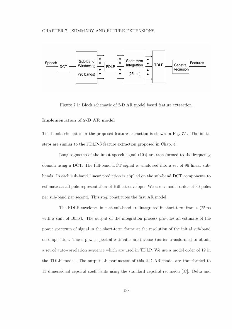
CHAPTER 7. SUMMARY AND FUTURE EXTENSIONS
Figure 7.1: Block schematic of 2-D AR model based feature extraction.
Implementation of 2-D AR model
The block schematic for the proposed feature extraction is shown in Fig. 7.1. The initial
steps are similar to the FDLP-S feature extraction proposed in Chap. 4.
Long segments of the input speech signal (10s) are transformed to the frequency
domain using a DCT. The full-band DCT signal is windowed into a set of 96 linear sub-
bands. In each sub-band, linear prediction is applied on the sub-band DCT components to
estimate an all-pole representation of Hilbert envelope. We use a model order of 30 poles
per sub-band per second. This step constitutes the first AR model.
The FDLP envelopes in each sub-band are integrated in short-term frames (25ms
with a shift of 10ms). The output of the integration process provides an estimate of the
power spectrum of signal in the short-term frame at the resolution of the initial sub-band
decomposition. These power spectral estimates are inverse Fourier transformed to obtain
a set of auto-correlation sequence which are used in TDLP. We use a model order of 12 in
the TDLP model. The output LP parameters of this 2-D AR model are transformed to
13 dimensional cepstral coefficients using the standard cepstral recursion [37]. Delta and
138
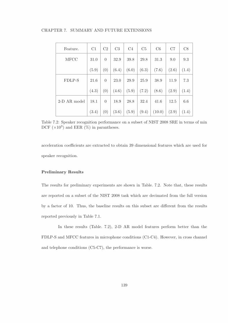
CHAPTER 7. SUMMARY AND FUTURE EXTENSIONS
Feature. C1 C2 C3 C4 C5 C6 C7 C8
MFCC 31.0 0 32.9 39.8 29.8 31.3 9.0 9.3
(5.9) (0) (6.4) (6.0) (6.3) (7.6) (2.6) (1.4)
FDLP-S 21.6 0 23.0 29.9 25.9 38.9 11.9 7.3
(4.3) (0) (4.6) (5.9) (7.2) (8.6) (2.9) (1.4)
2-D AR model 18.1 0 18.9 28.8 32.4 41.6 12.5 6.6
(3.4) (0) (3.6) (5.9) (9.4) (10.0) (2.9) (1.4)
Table 7.2: Speaker recognition performance on a subset of NIST 2008 SRE in terms of minDCF (×103) and EER (%) in parantheses.
acceleration coefficients are extracted to obtain 39 dimensional features which are used for
speaker recognition.
Preliminary Results
The results for preliminary experiments are shown in Table. 7.2. Note that, these results
are reported on a subset of the NIST 2008 task which are decimated from the full version
by a factor of 10. Thus, the baseline results on this subset are different from the results
reported previously in Table 7.1.
In these results (Table. 7.2), 2-D AR model features perform better than the
FDLP-S and MFCC features in microphone conditions (C1-C4). However, in cross channel
and telephone conditions (C5-C7), the performance is worse.
139
CHAPTER 7. SUMMARY AND FUTURE EXTENSIONS
Future Work
There is a scope for further extensions in terms of band-pass filtering the temporal and
spectral AR models. For example, human speech perception is sensitive to certain range of
temporal and spectral modulations [6]. This can be implemented in the 2-D AR model by
filtering the cepstral coefficients obtained from the spectral and temporal AR model. By
filtering these modulations, the 2-D AR model features can achieve robustness in noisy and
reverberant conditions.
7.5 Chapter Summary
In this chapter, we have outlined various contributions of this thesis (Sec. 7.2).
We have also described the limitations and scope of applicability of the FDLP approach in
Sec. 7.3. Finally, we discuss some extensions of the FDLP technique for feature extraction
as well as speech activity detection (Sec. 7.4).
140
Appendix A
Properties of Hilbert Transforms
A.1 Definition of the Linear Filter Model
In this section, we try to model the ideal Hilbert transform using the linear filter
model. Some of these properties are derived in [88]. We define the important properties of
required Hilbert transform H,
H[
cos(ω0t)]
= sin(ω0t) (A.1)
H[
sin(ω0t)]
= cos(ω0t) (A.2)
for any frequency ω0 of interest. Assuming the above operation can be modeled using a
linear filter, this can be written in the frequency domain1
δ(ω − ω0) + δ(ω + ω0)
×H(ω) = −j
δ(ω − ω0)− δ(ω + ω0)
(A.3)
δ(ω − ω0)− δ(ω + ω0)
×H(ω) = −j
δ(ω − ω0) + δ(ω + ω0)
(A.4)
1Here, we use Kronecker delta functions assuming the integrable nature of these functions. In a strictLebesgue sense, these function integrate to 0. However, we assume these impulse functions as the Fouriertransform of trigonometric functions.
141
APPENDIX A. PROPERTIES OF HILBERT TRANSFORMS
where we have used,
cos(ω0t)F⇐⇒ δ(ω − ω0) + δ(ω + ω0)
2
and
sin(ω0t)F⇐⇒ δ(ω − ω0)− δ(ω + ω0)
2j
and H(w) denotes the frequency response of the Hilbert transform filter. From Eq. A.3 and
Eq. A.4, we can write,
H(ω) =
j for ω < 0
−j for ω ≥ 0
(A.5)
In other words, H(ω) = −jSgn(ω). In the time domain the corresponding filter can be
obtained as,
h(t) =1
2π
∫ ∞
−∞−jSgn(ω)ejωtdω (A.6)
=1
2π
∫ 0
−∞jejωtdω −
∫ ∞
0jejωtdω
=1
πt
Thus, the Hilbert transform of a signal x(t) in the time domain can be written as,
H[
x(t)]
=1
π
∫ ∞
−∞
x(t− τ)
τdτ (A.7)
Since the above integral has a unbounded value at τ = 0, we define the Hilbert operator
using Cauchy principle value (CPV),
H[
x(t)]
= limǫ→0
1
π
[∫ ǫ
−∞
x(t− τ)
τdτ +
1
π
∫ ∞
ǫ
x(t− τ)
τdτ
]
(A.8)
142
APPENDIX A. PROPERTIES OF HILBERT TRANSFORMS
A.2 Hilbert Transform of a Cosine
In this section, we find the Hilbert transform, defined by Eq. A.7, of an input
signal x(t) = cos(t). Eq. A.7 can be re-written as,
H[cos(t)] =1
π
∫ ∞
−∞
cos(t− τ)
τdτ (A.9)
=1
πcos(t)
∫ ∞
−∞
cos(τ)
τdτ +
1
πsin(t)
∫ ∞
−∞
sin(τ)
τdτ
Now, since cosine is an even function and sine is an odd function we have,
∫ ∞
−∞
cos(τ)
τdτ = 0 (A.10)
∫ ∞
−∞
sin(τ)
τdτ = 2
∫ ∞
0
sin(τ)
τdτ
= 2
∫ ∞
0
∫ ∞
0e−sτsin(τ)dτds
where we have used 1τ=
∫∞0 e−sτds and we have assumed suitable properties for a change
of integral. Now, we need to show the Laplace transform of a sine function,
∫
sin(τ)e−sτdτ = cos(τ)e−sτ + s
∫
cos(τ)e−sτdτ (A.11)
= cos(τ)e−sτ − ssin(τ)e−sτ − s2∫
sin(τ)e−sτdτ
(1 + s2)
∫ ∞
0sin(τ)e−sτdτ = 1 (A.12)
(A.13)
where we have used integration by parts twice and evaluated the value of the integral using
the limits. Substituting Eq. A.12 in Eq. A.10, we get,
∫ ∞
−∞
sin(τ)
τdτ = 2
∫ ∞
0
1
1 + s2ds (A.14)
= 2
∫ π2
0
1
1 + tan2θsec2θdθ
= π (A.15)
143
APPENDIX A. PROPERTIES OF HILBERT TRANSFORMS
where we have used a substitution of variables s = tanθ. Now, substituting the value of
Eq. A.14 and Eq. A.10 in Eq. A.9, we arrive at the fundamental result,
H[cos(t)] = sin(t) (A.16)
This result satisfies the requirement of the Hilbert transform mentioned in Eq. A.1. A
similar proof can be shown for the Hilbert transform of a sine wave.
A.3 Analytic Signal for Convolution
Let r(t) be defined as,
r(t) = x(t) ∗ y(t), (A.17)
and let xa(t), ya(t) and ra(t) denote the analytic signal of x(t), y(t) and r(t) (defined using
the Eq. 2.3). Now,
ra(t) = r(t) + jH[r(t)] (A.18)
= x(t) ∗ y(t) + jx(t) ∗ y(t) ∗ h(t) (A.19)
where h(t) is the Hilbert filter defined in Eq. A.6. From Eq. A.5, we note that H(ω) =
−jSgn(ω). Then,
h(t) ∗ h(t) = F−1[
H(ω)H(ω)]
(A.20)
= −1
Combining Eq. A.20 and Eq. A.19 we can write,
ra(t) =1
2[x(t) ∗ y(t)]− 1
2[x(t) ∗ y(t) ∗ h(t) ∗ h(t)] + j
2
[
x(t) ∗ (y(t) ∗ h(t))]
+j
2
[
(x(t) ∗ h(t)) ∗ y(t)]
=1
2
[
x(t) + j(x(t) ∗ h(t))]
∗[
y(t) + j(y(t) ∗ h(t))]
(A.21)
144
APPENDIX A. PROPERTIES OF HILBERT TRANSFORMS
where we have split the two terms of Eq. A.19 into two halves and used the linearity and
associative property of convolution operator. Now, using Eq. A.7 and Eq. 2.3 we find that
x(t) + j(x(t) ∗ h(t)) = x(t) + jH[x(t)] = xa(t). Thus, Eq. A.21 can be simplified as
ra(t) =1
2xa(t) ∗ ya(t) (A.22)
Thus, the analytic signal of the convolved output is a equal to half of the convolution of
the individual analytic signals.
145
Appendix B
Minimum Phase Property of
Linear Prediction
In this chapter, we prove the minimum-phase property of linear prediction poly-
nomial. The minimum-phase property implies that all the roots of the linear prediction
polynomial lie inside the unit-circle.
The following proof is obtained from [89]. In this derivation, we use expectation
operator instead of summations for defining the auto-correlations, i.e. auto-correlation of a
discrete sequence x[n] is defined as,
rx[τ ] = E[
x[n]x[n− τ ]]
(B.1)
Let D(z) =∑p
k=0 akz−k denote the Z-transform of the optimal linear prediction filter ak
for k = 0, ... , p with a0 = 1. From the property of least squares optimization, the resulting
LP residual error is orthogonal to the past p samples of the input, i.e., let e[n] denote the
146
APPENDIX B. MINIMUM PHASE PROPERTY OF LINEAR PREDICTION
prediction error signal. Then, we have,
E[
e[n]x[n− k]]
= 0 (B.2)
for k = 1, ... , p. Let α denote any root of D(z) and let L(z) denote the polynomial removing
the zero at α, i.e., D(z) = (1− αz−1)L(z). Note that, L(z) denotes a p− 1 order filter. In
order to prove the minimum-phase property, we need to show |α| < 1, for every root α of
D(z).
Let u[n] denote the output when the signal x[n] is filtered with L(z). In other
words, since D(z) = (1− αz−1)L(z) and e[n] = x[n] ∗ d[n], we can write,
u[n] = l[n] ∗ x[n] =p−1∑
k=0
l[n]x[n− k] (B.3)
e[n] = u[n]− αu[n− 1] (B.4)
where L(z) =∑p−1
n=0 l[n]z−n with l[0] = 1. From the orthogonality property (Eq. B.2), we
note that,
E[
e[n]u[n− 1]]
= 0 (B.5)
Combining Eq. B.4 and Eq. B.5 gives
E[
u[n]− αu[n− 1]u[n− 1]]
= 0 (B.6)
ru[1] = αru[0] (B.7)
147
APPENDIX B. MINIMUM PHASE PROPERTY OF LINEAR PREDICTION
Further, using Eq. B.4, we can write the variance of the optimal LP error as,
E[
|e[n]|2]
= E[
e[n]u[n]− αu[n− 1]∗]
= E[
e[n]u∗[n]]
= E[
u[n]− αu[n− 1]u∗[n]]
= ru[0]− αr∗u[1]
= ru[0](1− |α|2) (B.8)
where we have used Eq. B.5 in the second step and Eq. B.7 in the last step and u∗ denotes
complex conjugation of u. Assuming that x[n] is not fully predictable, we have E[
|e[n]|2]
>
0. This would mean that (from Eq. B.8)
|α| < 1 (B.9)
Since this is true for any zero α, we have the minimum-phase property of the linear prediction
polynomial.
The minimum-phase property guarantees that the poles of the resulting LP power
spectrum lie inside the unit-circle in the complex frequency plane.
148
Appendix C
Two-Dimensional Representation
of Signals
C.1 Comparison of Spectrograms for Synthetic Signals
In Sec. 4.2.1, we have shown the FDLP spectrogram (Fig. 4.3) of a synthetic signal
plotted in Fig. 4.2. In this section, we show the corresponding spectrogram for various types
of STFT.
C.1.1 Wide-band spectrogram
The wide-band STFT spectrogram is obtained by 25 ms Hamming window with
a half overlap between neighboring frames. We use a 256 point DFT within each analysis
frame and plot the magnitude of STFT in each frame. These are stacked in a column manner
to obtain the plot shown in Fig. C.1. As seen in this figure, the wide-band spectrogram can
resolve the location of temporal spike with a good accuracy. However, the spectral locations
149
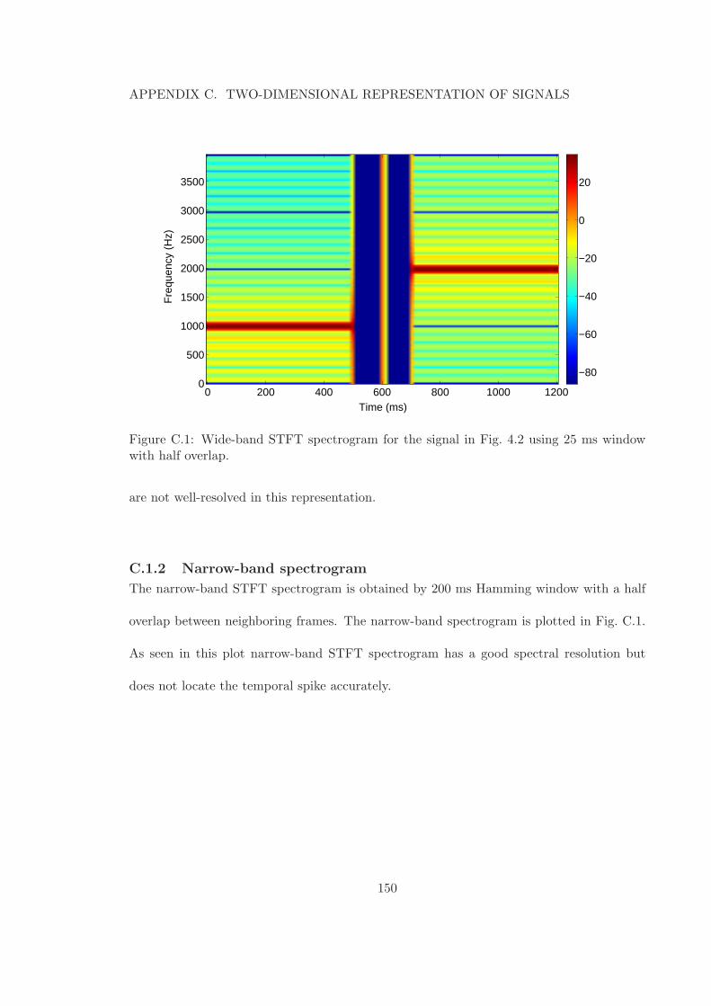
APPENDIX C. TWO-DIMENSIONAL REPRESENTATION OF SIGNALS
Time (ms)
Fre
quen
cy (
Hz)
0 200 400 600 800 1000 1200
3500
3000
2500
2000
1500
1000
500
0−80
−60
−40
−20
0
20
Figure C.1: Wide-band STFT spectrogram for the signal in Fig. 4.2 using 25 ms windowwith half overlap.
are not well-resolved in this representation.
C.1.2 Narrow-band spectrogram
The narrow-band STFT spectrogram is obtained by 200 ms Hamming window with a half
overlap between neighboring frames. The narrow-band spectrogram is plotted in Fig. C.1.
As seen in this plot narrow-band STFT spectrogram has a good spectral resolution but
does not locate the temporal spike accurately.
150
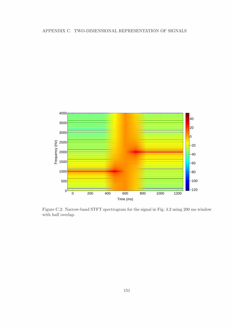
APPENDIX C. TWO-DIMENSIONAL REPRESENTATION OF SIGNALS
Time (ms)
Fre
quen
cy (
Hz)
0 200 400 600 800 1000 1200
4000
3500
3000
2500
2000
1500
1000
500
0 −120
−100
−80
−60
−40
−20
0
20
40
Figure C.2: Narrow-band STFT spectrogram for the signal in Fig. 4.2 using 200 ms windowwith half overlap.
151

Bibliography
[1] S. Davis and P. Mermelstein, “Comparison of parametric representations for monosyl-
labic word recognition in continuously spoken sentences,” Acoustics, Speech and Signal
Processing, IEEE Transactions on, vol. 28, no. 4, pp. 357–366, 1980.
[2] H. Hermansky, “Perceptual linear predictive (plp) analysis of speech,” Journal of the
Acoustical Society of America, vol. 87, no. 4, pp. 1738–1752, 1990.
[3] M. Bosi, K. Brandenburg, S. Quackenbush, L. Fielder, K. Akagiri, H. Fuchs, M. Di-
etz, J. Herre, G. Davidson, and Y. Oikawa, “Iso/iec mpeg-2 advanced audio coding,”
Journal of the Audio engineering society, vol. 45, no. 10, pp. 789–814, 1997.
[4] E. Ekudden, R. Hagen, I. Johansson, and J. Svedberg, “The adaptive multi-rate speech
coder,” in Speech Coding, IEEE Workshop on. IEEE, 1999, pp. 117–119.
[5] W. Thorpe, “The process of song-learning in the chaffinch as studied by means of the
sound spectrograph,” 1954.
[6] T. Chi, P. Ru, and S. Shamma, “Multiresolution spectrotemporal analysis of complex
sounds,” The Journal of the Acoustical Society of America, vol. 118, p. 887, 2005.
152
BIBLIOGRAPHY
[7] R. Drullman, J. Festen, and R. Plomp, “Effect of temporal envelope smearing on speech
reception,” Journal of the Acoustical Society of America, vol. 95, no. 2, pp. 1053–1064,
1994.
[8] ——, “Effect of reducing slow temporal modulations on speech reception,” Journal of
the Acoustical Society of America, vol. 95, no. 5, pp. 2670–2680, 1994.
[9] T. Arai, M. Pavel, H. Hermansky, and C. Avendano, “Intelligibility of speech with
filtered time trajectories of spectral envelopes,” in Spoken Language, 1996. ICSLP 96.
Proceedings., Fourth International Conference on, vol. 4. IEEE, 1996, pp. 2490–2493.
[10] R. Shannon, F. Zeng, V. Kamath, J. Wygonski, and M. Ekelid, “Speech recognition
with primarily temporal cues,” Science, vol. 270, no. 5234, p. 303, 1995.
[11] R. Ziemer and W. Tranter, Principles Of Communications: System Modulation And
Noise. Wiley, 2007.
[12] D. Gabor, “Theory of communication. part 1: The analysis of information,” Electrical
Engineers-Part III: Radio and Communication Engineering, Journal of the Institution
of, vol. 93, no. 26, pp. 429–441, 1946.
[13] G. Cain, “Hilbert-transform description of linear filtering,” Electronics Letters, vol. 8,
no. 15, pp. 380–382, 1972.
[14] A. Nuttall and E. Bedrosian, “On the quadrature approximation to the hilbert trans-
form of modulated signals,” Proceedings of the IEEE, vol. 54, no. 10, pp. 1458–1459,
1966.
153
BIBLIOGRAPHY
[15] D. Vakman, “On the analytic signal, the teager-kaiser energy algorithm, and other
methods for defining amplitude and frequency,” Signal Processing, IEEE Transactions
on, vol. 44, no. 4, pp. 791–797, 1996.
[16] H. Hermansky and N. Morgan, “Rasta processing of speech,” Speech and Audio Pro-
cessing, IEEE Transactions on, vol. 2, no. 4, pp. 578–589, 1994.
[17] J. Kaiser, “On a simple algorithm to calculate theenergy’of a signal,” in Acoustics,
Speech, and Signal Processing, 1990. ICASSP-90., 1990 International Conference on.
IEEE, 1990, pp. 381–384.
[18] P. Maragos, J. Kaiser, and T. Quatieri, “Energy separation in signal modulations with
application to speech analysis,” Signal Processing, IEEE Transactions on, vol. 41,
no. 10, pp. 3024–3051, 1993.
[19] P. Clark and L. Atlas, “Time-frequency coherent modulation filtering of nonstationary
signals,” Signal Processing, IEEE Transactions on, vol. 57, no. 11, pp. 4323–4332, 2009.
[20] T. Houtgast and H. Steeneken, “A review of the mtf concept in room acoustics and
its use for estimating speech intelligibility in auditoria,” The Journal of the Acoustical
Society of America, vol. 77, p. 1069, 1985.
[21] S. Furui, “Speaker-independent isolated word recognition using dynamic features of
speech spectrum,” Acoustics, Speech and Signal Processing, IEEE Transactions on,
vol. 34, no. 1, pp. 52–59, 1986.
[22] H. Hermansky and P. Fousek, “Multi-resolution rasta filtering for tandem-based asr,”
in Proceedings of Interspeech, vol. 2005. Citeseer, 2005.
154

BIBLIOGRAPHY
[23] B. Kingsbury, N. Morgan, and S. Greenberg, “Robust speech recognition using the
modulation spectrogram,” Speech Communication, vol. 25, no. 1-3, pp. 117–132, 1998.
[24] L. Atlas and C. Janssen, “Coherent modulation spectral filtering for single-channel mu-
sic source separation,” in Acoustics, Speech, and Signal Processing, 2005. Proceedings.
IEEE International Conference on, vol. 4. IEEE, 2005, pp. 461–464.
[25] S. Schimmel, L. Atlas, and K. Nie, “Feasibility of single channel speaker separation
based on modulation frequency analysis,” in Acoustics, Speech and Signal Processing,
2007. IEEE International Conference on, vol. 4. IEEE, 2007, pp. 605–608.
[26] R. Kumaresan and A. Rao, “Model-based approach to envelope and positive instan-
taneous frequency estimation of signals with speech applications,” The Journal of the
Acoustical Society of America, vol. 105, p. 1912, 1999.
[27] M. Athineos and D. Ellis, “Autoregressive modeling of temporal envelopes,” Signal
Processing, IEEE Transactions on, vol. 55, no. 11, pp. 5237–5245, 2007.
[28] S. Ganapathy, S. Thomas, P. Motlicek, and H. Hermansky, “Applications of signal
analysis using autoregressive models for amplitude modulation,” in Applications of
Signal Processing to Audio and Acoustics, 2009. WASPAA’09. IEEE Workshop on.
IEEE, pp. 341–344.
[29] J. Makhoul, “Linear prediction: A tutorial review,” Proceedings of the IEEE, vol. 63,
no. 4, pp. 561–580, 1975.
[30] J. Herre and J. Johnston, “Enhancing the performance of perceptual audio coders by
using temporal noise shaping (tns),” 101st AES Convention.
155
BIBLIOGRAPHY
[31] S. Martucci, “Symmetric convolution and the discrete sine and cosine transforms,”
Signal Processing, IEEE Transactions on, vol. 42, no. 5, pp. 1038–1051, 1994.
[32] H. Voelcker, “Toward a unified theory of modulation part i: Phase-envelope relation-
ships,” Proceedings of the IEEE, vol. 54, no. 3, pp. 340–353, 1966.
[33] R. Kumaresan, “An inverse signal approach to computing the envelope of a real valued
signal,” Signal Processing Letters, IEEE, vol. 5, no. 10, pp. 256–259, 1998.
[34] M. Athineos and D. Ellis, “Frequency-domain linear prediction for temporal features,”
in Automatic Speech Recognition and Understanding, 2003. ASRU’03. 2003 IEEE
Workshop on. IEEE, 2003, pp. 261–266.
[35] L. Marple Jr, “Computing the discrete-time analytic signal via fft,” Signal Processing,
IEEE Transactions on, vol. 47, no. 9, pp. 2600–2603, 1999.
[36] M. Athineos, H. Hermansky, and D. Ellis, “Lp-trap: Linear predictive temporal pat-
terns,” in Eighth International Conference on Spoken Language Processing, 2004.
[37] B. Atal and S. Hanauer, “Speech analysis and synthesis by linear prediction of the
speech wave,” The Journal of the Acoustical Society of America, vol. 50, p. 637, 1971.
[38] H. Hsu and C. Liu, “Autoregressive modeling of temporal/spectral envelopes with
finite-length discrete trigonometric transforms,” Signal Processing, IEEE Transactions
on, vol. 58, no. 7, pp. 3692–3705, 2010.
[39] A. Rosenberg, C. Lee, and F. Soong, “Cepstral channel normalization techniques for
156
BIBLIOGRAPHY
hmm-based speaker verification,” in Third International Conference on Spoken Lan-
guage Processing, 1994.
[40] C. Avendano and H. Hermansky, “On the effects of short-term spectrum smoothing in
channel normalization,” Speech and Audio Processing, IEEE Transactions on, vol. 5,
no. 4, pp. 372–374, 1997.
[41] D. Gelbart and N. Morgan, “Evaluating long-term spectral subtraction for reverber-
ant asr,” in Automatic Speech Recognition and Understanding, 2001. ASRU’01. IEEE
Workshop on. IEEE, 2001, pp. 103–106.
[42] J. Mourjopoulos and J. Hammond, “Modelling and enhancement of reverberant speech
using an envelope convolution method,” in Acoustics, Speech, and Signal Processing,
IEEE International Conference on ICASSP’83., vol. 8. IEEE, 1983, pp. 1144–1147.
[43] S. Thomas, S. Ganapathy, and H. Hermansky, “Recognition of reverberant speech
using frequency domain linear prediction,” Signal Processing Letters, IEEE, vol. 15,
pp. 681–684, 2008.
[44] D. Pearce and H. Hirsch, “The aurora experimental framework for the performance
evaluation of speech recognition systems under noisy conditions,” in Proc. ICSLP00,
vol. 4. ISCA, 2000, pp. 29–32.
[45] P. Pierce and A. Gunawardana, “Aurora 2.0 speech recognition in noise: Update 2,”
in Proceedings of Interspeech. ISCA, 2002.
[46] G. S. Mallidi, H. and H. Hermansky, “Modulation spectrum analysis for recognition of
reverberant speech,” in Proceedings of Interspeech, 2011.
157
BIBLIOGRAPHY
[47] H. Hermansky, H. Fujisaki, and Y. Sato, “Analysis and synthesis of speech based on
spectral transform linear predictive method,” in Acoustics, Speech, and Signal Process-
ing, IEEE International Conference on ICASSP’83., vol. 8. IEEE, 1983, pp. 777–780.
[48] S. Thomas, S. Ganapathy, and H. Hermansky, “Hilbert envelope based features for far-
field speech recognition,” Machine Learning for Multimodal Interaction, pp. 119–124,
2008.
[49] S. Ganapathy, J. Pelecanos, and M. Omar, “Feature normalization for speaker verifi-
cation in room reverberation,” in Proc of ICASSP, 2011.
[50] J. Pelecanos and S. Sridharan, “Feature warping for robust speaker verification,” in
2001: A Speaker Odyssey-The Speaker Recognition Workshop, 2001.
[51] D. Reynolds, T. Quatieri, and R. Dunn, “Speaker verification using adapted gaussian
mixture models,” Digital signal processing, vol. 10, no. 1-3, pp. 19–41, 2000.
[52] W. Campbell, D. Sturim, D. Reynolds, and A. Solomonoff, “Svm based speaker verifi-
cation using a gmm supervector kernel and nap variability compensation,” in Acoustics,
Speech and Signal Processing, 2006. ICASSP 2006 Proceedings. 2006 IEEE Interna-
tional Conference on, vol. 1. IEEE, 2006, pp. I–I.
[53] A. Hatch, S. Kajarekar, and A. Stolcke, “Within-class covariance normalization for
svm-based speaker recognition,” in Ninth International Conference on Spoken Lan-
guage Processing, 2006.
[54] R. Auckenthaler, M. Carey, and H. Lloyd-Thomas, “Score normalization for text-
158
BIBLIOGRAPHY
independent speaker verification systems,” Digital Signal Processing, vol. 10, no. 1-3,
pp. 42–54, 2000.
[55] S. Ganapathy, S. Thomas, and H. Hermansky, “Modulation frequency features for
phoneme recognition in noisy speech,” 2009.
[56] T. Dau, D. Puschel, and A. Kohlrausch, “A quantitative model of the effective signal
processing in the auditory system. i. model structure,” Journal of the Acoustical Society
of America, vol. 99, no. 6, pp. 3615–3622, 1996.
[57] J. Tchorz and B. Kollmeier, “A model of auditory perception as front end for automatic
speech recognition,” The Journal of the Acoustical Society of America, vol. 106, p. 2040,
1999.
[58] H. Bourlard and N. Morgan, Connectionist speech recognition: a hybrid approach.
Springer, 1994.
[59] K. Lee and H. Hon, “Speaker-independent phone recognition using hidden markov mod-
els,” Acoustics, Speech and Signal Processing, IEEE Transactions on, vol. 37, no. 11,
pp. 1641–1648, 1989.
[60] J. Pinto, B. Yegnanarayana, H. Hermansky, and M. Magimai-Doss, “Exploiting contex-
tual information for improved phoneme recognition,” in Acoustics, Speech and Signal
Processing, 2008. ICASSP 2008. IEEE International Conference on. IEEE, 2008, pp.
4449–4452.
[61] T. Hain and L. e. a. Burget, “The development of the ami system for the transcription
159
BIBLIOGRAPHY
of speech in meetings,” Machine Learning for Multimodal Interaction, pp. 344–356,
2006.
[62] S. Ganapathy, S. Thomas, and H. Hermansky, “Comparison of modulation features
for phoneme recognition,” in Acoustics Speech and Signal Processing (ICASSP), 2010
IEEE International Conference on. IEEE, 2010, pp. 5038–5041.
[63] V. Tyagi and C. Wellekens, “Fepstrum representation of speech signal,” in Automatic
Speech Recognition and Understanding, 2005 IEEE Workshop on. IEEE, 2005, pp.
11–16.
[64] E. Standard, “Etsi es 202 050 v1.1.1 stq; distributed speech recognition; advanced
front-end feature extraction algorithm; compression algorithms,” 2002.
[65] Y. Ephraim and D. Malah, “Speech enhancement using a minimum-mean square error
short-time spectral amplitude estimator,” Acoustics, Speech and Signal Processing,
IEEE Transactions on, vol. 32, no. 6, pp. 1109–1121, 1984.
[66] S. Ganapathy, S. Thomas, and H. Hermansky, “Temporal envelope compensation for
robust phoneme recognition using modulation spectrum,” The Journal of the Acoustical
Society of America, vol. 128, no. 6, pp. 3769–3780, 2010.
[67] H. Hirsch and H. Finster, “The simulation of realistic acoustic input scenarios for
speech recognition systems,” in Ninth European Conference on Speech Communication
and Technology, 2005.
[68] D. Reynolds, “Htimit and llhdb: speech corpora for the study of handset transducer
160
BIBLIOGRAPHY
effects,” in Acoustics, Speech, and Signal Processing, 1997. ICASSP-97., 1997 IEEE
International Conference on, vol. 2. IEEE, 1997, pp. 1535–1538.
[69] C. Chen and J. Bilmes, “Mva processing of speech features,” Audio, Speech, and Lan-
guage Processing, IEEE Transactions on, vol. 15, no. 1, pp. 257–270, 2007.
[70] Y. Shao, Z. Jin, D. Wang, and S. Srinivasan, “An auditory-based feature for robust
speech recognition,” in Acoustics, Speech and Signal Processing, 2009. ICASSP 2009.
IEEE International Conference on. IEEE, 2009, pp. 4625–4628.
[71] I. JTC1/SC29/WG11, “Call for proposals on unified speech and audio coding,” 2007.
[72] S. Ganapathy, P. Motlicek, and H. Hermansky, “Autoregressive models of amplitude
modulations in audio compression,” Audio, Speech, and Language Processing, IEEE
Transactions on, vol. 18, no. 6, pp. 1624–1631, 2010.
[73] P. Motlıcek, S. Ganapathy, H. Hermansky, H. Garudadri, and M. Athineos, “Percep-
tually motivated sub-band decomposition for fdlp audio coding,” in Text, Speech and
Dialogue. Springer, 2008, pp. 435–442.
[74] X. Xie, S. Chan, and T. Yuk, “M-band perfect-reconstruction linear-phase filter banks,”
in Statistical Signal Processing, 2001. Proceedings of the 11th IEEE Signal Processing
Workshop on. IEEE, 2001, pp. 583–586.
[75] J. Princen, A. Johnson, and A. Bradley, “Subband/transform coding using filter bank
designs based on time domain aliasing cancellation,” in Acoustics, Speech, and Signal
Processing, IEEE International Conference on ICASSP’87., vol. 12. IEEE, 1987, pp.
2161–2164.
161
BIBLIOGRAPHY
[76] S. Ganapathy, P. Motlicek, H. Hermansky, and H. Garudadri, “Temporal masking
for bit-rate reduction in audio codec based on frequency domain linear prediction,”
in Acoustics, Speech and Signal Processing, 2008. ICASSP 2008. IEEE International
Conference on. IEEE, 2008, pp. 4781–4784.
[77] ——, “Spectral noise shaping: Improvements in speech/audio codec based on linear
prediction in spectral domain,” in Ninth Annual Conference of the International Speech
Communication Association, 2008.
[78] W. Jesteadt, S. Bacon, and J. Lehman, “Forward masking as a function of frequency,
masker level, and signal delay,” The journal of the Acoustical Society of America,
vol. 71, p. 950, 1982.
[79] F. Sinaga, T. Gunawan, and E. Ambikairajah, “Wavelet packet based audio coding us-
ing temporal masking,” in Information, Communications and Signal Processing, 2003
and the Fourth Pacific Rim Conference on Multimedia. Proceedings of the 2003 Joint
Conference of the Fourth International Conference on, vol. 3. IEEE, pp. 1380–1383.
[80] I. JTC1/SC29/WG11, “Framework for exploration of speech and audio coding,” 2007.
[81] G. T. 26.401, “Enhanced aacplus general audio codec; general description.”
[82] M. Dietz, L. Liljeryd, K. Kjorling, and O. Kunz, “Spectral band replication, a novel
approach in audio coding,” PREPRINTS-AUDIO ENGINEERING SOCIETY, 2002.
[83] I.-R. R. BS.1387, “Method for objective psychoacoustic model based on peaq to per-
ceptual audio measurements of perceived audio quality,” 1998.
162
BIBLIOGRAPHY
[84] I.-R. R. BS.1534:, “Method for the subjective assessment of intermediate audio quality,”
2001.
[85] S. Ganapathy, P. Motlicek, and H. Hermansky, “Autoregressive modelling of hilbert
envelopes for wide-band audio coding,” 2008.
[86] T. Kinnunen, K. Lee, and H. Li, “Dimension reduction of the modulation spectrogram
for speaker verification.” The Speaker and Language Recognition Workshop (Odyssey
2008).
[87] M. Athineos, H. Hermansky, and E. D., “Plp-2 autoregressive modeling of auditory-like
2-d spectro-temporal patterns,” ISCA Tutorial and Research Workshop on Statistical
and Perceptual Audio Processing SAPA-04.
[88] S. Clay, “Hilbert transforms, analytic functions, and analytic signals,” personal.atl.
bellsouth.net/p/h/physics/hilberttransforms.pdf.
[89] P. Vaidyanathan, J. Tuqan, and A. Kirac, “On the minimum phase property of
prediction-error polynomials,” Signal Processing Letters, IEEE, vol. 4, no. 5, pp. 126–
127, 1997.
163
Vita
Sriram Ganapathy received his Bachelor of Technology degree in Electronics
and Communications from College of Engineering, Trivandrum, India in 2004 and
Master of Engg. degree in Signal Processing from Indian Institute of Science, Banga-
lore in 2006. He completed his PhD. from Center of Language and Speech Processing
(CLSP), Johns Hopkins University in 2011. Currently, he is a post-doctoral researcher
at IBM T.J. Watson Reseach Center, Yorktown Heights. His is primarily interested in
developing long-term signal models for speech and audio processing. He has worked
as a Research Assistant in Idiap Research Institute, Switzerland from 2006 to 2008.
His research interests include signal processing, machine learning, robust speech and
speaker recognition.
164