Short Comments on Continuum Mechanics: Theory and Computation

Short Comments on Continuum Mechanics: Theory andComputation

G. Linga, J. Mathiesen, B. F. Nielsen

Version: 13th March 2019

1

Continuum mechanics G. Linga, J. Mathiesen, B. F. Nielsen

Contents

1 Week 1 31.1 Traction or stress vector . . . . . . . . . . . . . . . . . . . . . . . . . . . . . . . . . 31.2 Force balance . . . . . . . . . . . . . . . . . . . . . . . . . . . . . . . . . . . . . . . 61.3 Strain . . . . . . . . . . . . . . . . . . . . . . . . . . . . . . . . . . . . . . . . . . . 71.4 The Euler Strain Tensor . . . . . . . . . . . . . . . . . . . . . . . . . . . . . . . . . 8

2 Week 2 92.1 Hooke’s law and the Navier-Cauchy equation . . . . . . . . . . . . . . . . . . . . . . 92.2 Elastic energy . . . . . . . . . . . . . . . . . . . . . . . . . . . . . . . . . . . . . . . 102.3 Linear elastodynamics from Harmonic Oscillators . . . . . . . . . . . . . . . . . . . 11

2.3.1 Material Parameters in Linear Elasticity . . . . . . . . . . . . . . . . . . . . 132.4 Reynold’s Transport Theorem . . . . . . . . . . . . . . . . . . . . . . . . . . . . . . 14

3 Week 3 163.1 Balance laws . . . . . . . . . . . . . . . . . . . . . . . . . . . . . . . . . . . . . . . . 163.2 The temporal elasticity equation . . . . . . . . . . . . . . . . . . . . . . . . . . . . . 17

4 Week 4 184.1 Ideal and nearly ideal flow . . . . . . . . . . . . . . . . . . . . . . . . . . . . . . . . 184.2 Potential flow . . . . . . . . . . . . . . . . . . . . . . . . . . . . . . . . . . . . . . . 19

5 Week 5 215.1 Solutions to Stokes’ First and Second Problem . . . . . . . . . . . . . . . . . . . . . 21

6 Week 6 246.1 Stokes flow . . . . . . . . . . . . . . . . . . . . . . . . . . . . . . . . . . . . . . . . . 246.2 Finite Element Method . . . . . . . . . . . . . . . . . . . . . . . . . . . . . . . . . . 256.3 FEniCS/DOLFIN . . . . . . . . . . . . . . . . . . . . . . . . . . . . . . . . . . . . . 266.4 Getting started with FEniCS . . . . . . . . . . . . . . . . . . . . . . . . . . . . . . 27

6.4.1 Pipe flow . . . . . . . . . . . . . . . . . . . . . . . . . . . . . . . . . . . . . 276.5 Flow around objects . . . . . . . . . . . . . . . . . . . . . . . . . . . . . . . . . . . 336.6 Lid-driven cavity . . . . . . . . . . . . . . . . . . . . . . . . . . . . . . . . . . . . . 36

A Tensor subtleties (covered in week 2) 38

2


Introduction

Throughout the lectures, where not stated otherwise, I use the Einstein summation conventionwhere an index appearing twice in a single term implies summation, for example a scalar productbetween two vectors is written

a · b =3∑i=1

aibi = aibi, (1)

where ai and bi are the i’th components of the vectors a and b, respectively. A vector a can bewritten as

a = aiei, (2)

where ei is a unit vector in a given Cartesian coordinate system. Similarly a tensor σσσ can be writtenon the form

σσσ = σijei ⊗ ej (3)

or simply just as σij. In matrix notation, the dyadic product ei ⊗ ej is equivalent to the (i, j)’thentry of the matrix. In ”bra-ket” notation you could write a tensor entry ei ⊗ ej as

|ei〉〈ej|

1 Week 1

1.1 Traction or stress vector

The stress vector or traction vector, T(n), denotes the force acting on a cross-section, ∆S, with asurface normal n divided by the area of the cross section,

T(n) = lim∆S→0

∆F

∆S=∂F

∂S(4)

Consider a small rectangular box with vanishingly smallside areas, mass dm, and top and bottom areas dA. Theacceleration, a of the box must be proportional to thesum of all forces on the box, i.e.

adm = dA(T(n) + T(−n)

). (5)

In the case where the box is at rest, the sum of the tractionon the right-hand side of the equation must vanish, i.e.

T(n) = −T(−n) (6)

Therefore, the traction vectors on opposite sides of an interface or a flat mass element in rest mustbe of equal magnitude and point in opposite directions.

3


Cauchy’s stress hypothesis

Instead of a thin box, we now consider the force balance on a small tetrahedron, where, in the caseof no body forces, the surface forces acting on the four sides balances with the inertial force.

x

y

z

T(−ez)

T(−ex)

T(−ey)

n

T(n)

We therefore achieve the relation

ρdV a = T(−ex)dSx + T(−ey)dSy + T(−ez)dSz + T(n)dS

= −T(ex)dSx −T(ey)dSy −T(ez)dSz + T(n)dS

=(−T(ex)nx −T(ey)ny −T(ez)nz + T(n)

)dS. (7)

Here ρ denotes the mass density and dV is the volume of the tetrahedron. Furthermore, we usethe shorthand notation for the individual areas of the sides, dSi = ei · ndS. If we shrink thevolume equally in all directions such that we do not change it’s shape and let the linear scale ofthe tetrahedron go to zero, we have that the surface forces will dominate over the volume forces.If we denote the approximate linear size of the tetrahedron `, the area of a side element will beproportional to `2 and the volume proportional to `3, i.e. the volume divided by the area will beproportional to `. Neglecting the volume terms in Eq. (7), we end up with the relation

T(n) = T(ex)nx + T(ey)ny + T(ez)nz. (8)

In a more formal way, we could also write this as

T(n) =

(∑i

T(ei) ⊗ ei

)︸︷︷︸

The stress tensor σσσ

·n, (9)

where it now becomes clear that the traction on an arbitrary interface with normal n is a sum overthe tractions T(ei) weighted with the projections ei ·n. In index notation, we can write the tractionvector,

T(n)i = σijnj (10)

4


Similarly, we can also compute the normal stress acting on the surface by projecting T(n) onto n,i.e.

σnn = n ·T(n) = niT(n)i = niσijnj (11)

Example: Traction vector in 2D

x

y

T(ex)

S

S ′

n′

Assume that we have a traction, T(ex), acting on a surface perpendicular to the x-axis.

T(ex) = σ0ex. (12)

From the traction vector, we find that

σxx = ex ·T(ex) = σ0, σyx = ey ·T(ex) = 0 (13)

If we assume that no force is acting on the surface perpendicular to the y-axis, we achieve astress tensor on the form

σ =

(σ0 00 0

)(14)

We now consider the corresponding traction vector acting on the surface S ′ (representedby the dashed line in the figure) with surface normal ex′ = 1/

√2(ex + ey) and tangent

ey′ = 1/√

2(−ex + ey).The traction can be computed by going back to first principles, i.e. using (4)

T(ex′ ) = lim∆S′→0

σ0ex∆S

∆S ′=σ0ex√

2. (15)

Alternatively we may use (9) and compute the traction T(ey′ ) as

T(ey′ ) = T(ex)(ex · ey′) + T(ey)(ey · ey′) = −σ0ex√2. (16)

Expressing this in the frame of x′ and y′, we have that

T(ex′ ) =σ0

2

(ex′ + ey′

), T(ey′ ) =

σ0

2

(ex′ + ey′

). (17)

5


In this new frame, we can also calculate the stress tensor components

σx′x′ = ex′ ·T(ex′ ) =σ0

2, σy′x′ = ey′ ·T(ex′ ) =

σ0

2. (18)

σ′ =σ0

2

(1 11 1

)(19)

By performing a rotation, R(θ), of frame by an angle θ = π/4, one can verify (do it) that

σ = R(θ)σ′R(−θ) (20)

Remember that

R(θ) =

(cos θ − sin θsin θ cos θ

)(21)

Exercise

For the following stress tensor calculate the traction on a surface with a normal n(θ) fordifferent angles θ. The angle should be measured between the normal and the positive x-axis,

σ =σ0

2

(1 22 1

)(22)

1.2 Force balance

We write the total force acting on a body as a sum of body forces Fbody and surface forces Fsurface,

Ftotal = Fsurface + Fbody. (23)

The surface force is given by a surface integral of the traction vector T(n)

fsurface =

∮S

T(n)dS (24)

We now consider the force in the i’th direction and by inserting Eq. (10), the surface integralassumes the form

Fsurface,i =

∮S

T(n)i dS =

∮S

σijnjdS. (25)

By use of the divergence theorem the surface integral can be written as a volume integral,

Fsurface,i =

∫V

∂jσijdV. (26)

6


If we write the body force in terms of a force density

Fbody,i =

∫V

fbody,i dV, (27)

we achieve the following expression for the total force in the i’th direction

Ftotal,i =

∫V

fbody,i + ∂jσij dV, (28)

If the body is everywhere in mechanical equilibrium, we must have that for any volume over whichwe integrate the total force vanishes, we therefore have the following force balance condition atmechanical equilibrium,

0 = fbody,i + ∂jσij, (29)

Exercise

Pressure is always acting normal to a surface. For example if you rotate an object in yourhand, the atmospheric pressure p acting on a given surface element will not change. Thecorresponding traction can therefore be written on the form

T(n)i = −pni

If we now have a constant pressure acting everywhere on an object and we neglect any bodyforce, show that the Ftotal = 0.

1.3 Strain

Xi

Xj

Xi

xixj

Referencestate

Deformedstate

x = f(X)

Figure 1: Mapping between a materialreference state, described by a coordin-ate X, and a deformed state describedby a coordinate x.

Deformation and stress go hand in hand, however, in orderto formalize the relationship between them, we need a wayto describe deformation. We shall in the following definestrain for objects, which are only deformed minutely, saytypically less than a percent. For example, many con-struction materials will only sustain a minute degree ofdeformation before yielding. For those materials it is of-ten sufficient to only consider a linearized description ofdeformation. That being said, materials like rubber cansustain large deformation without yielding and do in facthave a highly non-trivial stress and strain relations. In theformalism of deformation, it is convenient to introduce areference state, which we here assume to be undeformed

7


and stress free1. The reference or material state is de-scribed by a Cartesian coordinate X and the deformedstate with a coordinate x. The deformation map (bijective function) between the two states isdenoted

x = f(X). (30)

If an object is moved and deformed relative to the reference state, each point will be displaced anew point in the deformed frame by a displacement vector field, which in the so-called Euleriandescription has the form

u(x) ≡ x−X(x) = x− f−1(x). (31)

Note that in this description, the reference coordinate is considered to be a function of the deformedcoordinate and that the displacement vector points from the reference coordinate to the deformedcoordinate.

1.4 The Euler Strain Tensor

X1x1

dxdX

X2

x2

f(X)

Figure 2: Transformation of a vectordX by the deformational map f(X).

During deformation, the distance vector between two in-finitesimally close material points in the reference frame,e.g. dX = X2−X1, is changed into a new distance vectordx = x2 − x1. The change in length of these elementsdL2 = dX ·dX and d`2 = dx ·dx is computed by first per-forming an expansion to linear order of the map followingEq. (30)

dXi ≈f−1i

∂x`dx`.

We now replace the individual coordinates in the configuration state by this expansion and achieve

dxidxi − dXidXi = dxidxi −∂f−1

i

∂x`

∂f−1i

∂xkdx`dxk

=

(δk` −

∂f−1i

∂x`

∂f−1i

∂xk

)dx`dxk

If we further apply the derivative to Eq. (31) and replace the map by the displacement field, weobtain

dxidxi − dXidXi =

(δk` −

[δik −

∂ui∂xk

] [δi` −

∂ui∂x`

])dxkdx`

=

(∂u`∂xk

+∂uk∂x`− ∂ui∂xk

∂ui∂x`

)dxkdx`

= 2uk`dxkdx` (32)

1More generally, we could develop a description where the reference state can have stress and be deformed.

8


Where we in the latter have introduced the symmetric strain tensor given by

uij =1

2

(∂uj∂xi

+∂ui∂xj− ∂un∂xi

∂un∂xj

)(33)

Throughout the course, we will generally neglect the non-linear terms and only consider the linearstrain tensor

uij =1

2

(∂uj∂xi

+∂ui∂xj

)(34)

2 Week 2

2.1 Hooke’s law and the Navier-Cauchy equation

For linear elasticity, the stress is assumed to be a linear combination of strain components (ukl)

σij = Eijklukl (35)

The fourth order tensor, Eijkl, relating the stress and strain tensor components is called the stiffnesstensor. It tells you how a strain ukl affects the stress component σij. For a fully isotropic medium,in which an applied stress (or strain) will give rise to the same strain (or stress) state, regardlessof the direction of application, the stiffness tensor can involve only two types of contributions:

• A pressure-like term λδijδkl giving nonzero components of the form E1111, E1122, E2222 etc.

• A term of the form µδikδjl which ensures that e.g. a strain of the form u12 also gives rise toa nonzero stress σ12 but not a stress in some other direction (e.g. σ13), which would be anexample of anisotropy

This latter term must in fact be symmetrized since the stress and strain tensors are symmetric, sothe full isotropic stiffness tensor becomes

Eijkl = µ(δikδjl + δjkδil) + λδijδkl. (36)

You may then verify that stress is related to the strain by

σij = 2µuij + λδijukk (37)

If we now consider the case of infinitesimal strains, where the strain tensor is given by Eq. (34), wearrive at the Navier-Cauchy equation by combining Eqs. (29), (37) and (34),

0 = µ∇2u + (µ+ λ)∇(∇ · u) (38)

In numerical solutions of the mechanical forces in a deformed elactic body, we can either try tosolve directly for the stress tensor using Eq. (29) or solve for the displacement using Eq. (95)

9


2.2 Elastic energy

The change in the internal energy ε of our elastic system follows from thermodynamics and assumesthe form

dε = Tds+ σijduij (39)

The first term is the usual thermal contribution to the energy while the last term represents thework done when the material undergoes strain. Think of it as ”mechanical work equals force timesdistance”.In solving real problems it is in many cases more convenient to consider the free energy, whichassumes the form

f = ε− Ts. (40)

By combining Eqs.(39) and (40), we arrive at an expression for the change in free energy

df = −sdT + σijduij (41)

Under the assumption of constant temperature, we may calculate the stress by the following ex-pression

σij =

(∂f

∂uij

)T=const

(42)

Next we assume that the free energy is always positive and isotropic and of maximum second order.For a general stiffness tensor Eijkl this leads to the expression

f =1

2Eijkluijukl, (43)

which can readily be checked to be in agreement with the linear stress-strain relation σij = Eijkluklby using (42).For linear isotropic materials this reduces to the following expression for the free energy

f =1

2λ(uii)

2 + µu2ij =

1

2λTr(u)2 + µu2

ij (44)

Again, this is consistent with Hooke’s law when using (42). As is evident from the above equation,the free energy is a homogeneous function of second order.

Homogeneous functions

A function f(x, y) is said to the homogeneous of order n if it satisfies the relation

f(tx, ty) = tnf(x, y) (45)

10


By differentiating on both sides with regards to t we get from the right-hand side

d

dttnf(x, y) = ntn−1f(x, y) (46)

and from the left-hand side

d

dtf(tx, ty) =

∂f

∂(tx)

∂tx

∂t+

∂f

∂(ty)

∂ty

∂t= x

∂f

∂(tx)+ y

∂f

∂(ty)(47)

By equating the two above equations and setting t = 1, we arrive at another relation satisfiedby homogeneous function.

nf(x, y) = x∂xf(x, y) + y∂yf(x, y). (48)

More generally, for a function f of several indexed variables xi the relation reads

nf = xi∂f

∂xi. (49)

Using that the free energy is of second order, we may use (49) to write

2f = uij∂f

∂uij(50)

In combination with Eq. (42) we then achieve the final expression for the free energy density foran elastic material (under constant temperature)

f =1

2σijuij (51)

2.3 Linear elastodynamics from Harmonic Oscillators

In this section we will consider a long series of springs, but let us start by recalling the mechanicsof combining springs in parallel and in series.For two springs with spring constants k1 and k2 connected in parallel, the total force is the sum ofthe forces exerted by each spring

Kx = k1x1 + k2x2 (52)

where K is the effective (total) spring constant.When connected in parallel, the extension of each spring must equal the total extension of thesystem, i.e. x1 = x2 = x. We thus find

K = k1 + k2. (53)

11


This is of course easily generalized to an arbitrary number N of springs:

K =N∑i=1

ki, (Parallel). (54)

For springs in series, each spring is pulled by the same force of magnitude F and their extensionis then given by xi = F/ki. Furthermore the total extension of the spring system is the sum of theindividual extensions:

F = Kx = K(x1 + x2) = K

(F

k1

+F

k2

)⇒ 1 = K

(1

k1

+1

k2

). (55)

This then leads to the effective (total) spring constant K given by

K =1

1k1

+ 1k2

. (56)

Again, this is easily generalized to an N -spring system

K =1∑N

i=1 k−1i

, (Series). (57)

For the special case of identical springs k1 = k2 = · · · = kN := k, we then just find

K =k

N, (Series, N identical springs). (58)

Consider now a series of springs, each of equilibrium length èq and individual spring constants k.The equilibrium length of the entire spring system is Leq. We may then use the above relation tofind the effective spring constant:

K =k

N=èq

Leq

k. (59)

The extension of the entire spring is of course proportional to the extensions of the individualsprings:

∆L := L− Leq = N(`− èq) =: N∆`. (60)

We let the equilibrium positions of the springs be xi, such that xi+1 = xi + `. When perturbed, thesprings will of course be displaced in a time-dependent manner. We let ui(x, t) be the displacement,i.e.

xi → xi + ui(x, t). (61)

12


Then Newtons’s second law combined with Hooke’s Law gives

m∂2ui∂t2

= k(∆ui+1 −∆ui), (62)

where ∆ui means ui − ui−1. We thus find

m∂2ui∂t2

= k(ui+1 − 2ui + ui−1). (63)

Now, recall that the second derivative can be computed as

f ′′(x) = limh→0

f(x+ h)− 2f(x) + f(x− h)

h2. (64)

We can take the continuum limit by treating ui as a continuous variable and letting èq be small.This means

ui+1 − 2ui + ui−1 → u(x+ èq)− 2u(x) + u(x− èq) ≈ `2eq

∂2u

∂x2. (65)

In the continuum limit we thus find

∂2u

∂t2=k`2

eq

m

∂2u

∂x2. (66)

By comparison with the wave equation, we find a speed of sound (disturbance propagation speed)in this elastic medium of

cs = èq

√k

m. (67)

If we assume each mass to have a cross-sectional area A, the mass density is ρ = mAèq

. In this case

the speed of sound may be expressed as

cs =

√E

ρ. (68)

where E is Young’s Modulus which is – as we shall argue in a moment – a material parameter.Young’s modulus is, in general, defined as the tensile stress per unit of relative strain. In the presentcase, the relation is simply

E =kèq

A. (69)

2.3.1 Material Parameters in Linear Elasticity

There are two material parameters relevant to linear elasticity.

13


Young’s Modulus describes how hard it is to stretch a material in the direction you apply theforce (here: the x-direction):

E =σxxuxx

. (70)

This is a sensible material parameter because

• uxx is independent of the absolute length (as opposed to e.g. ux).

• σxx is ’force per area’, but the effective spring constant K ∝ A and so σxx is independent ofcross sectional area.

The relation between the spring constant and Young’s modulus can be worked out as

E =σxxuxx

=F/A

∆x/L=K∆xL

A∆x=KL

A. (71)

Since K ∝ A and K ∝ 1/L it is evident that E is indeed a material parameter, depending only onthe intrinsic properties of the material.

Poisson’s Ratio parametrizes how much a material expands/contracts in the transverse directionwhen stretched. Imagine that the material is stretched by a strain uxx and the transverse directionof interest is the y-direction. Then Poisson’s ratio ν is given by

ν = −uyyuxx

. (72)

In a linearly elastic material, both the denominator and numerator will be proportional to F , whichthen drops out and leaves us with a sensible material parameter.

2.4 Reynold’s Transport Theorem

Consider a global quantity Q which can be computed from an integral of a corresponding volumetricdensity q(x, t)

Q =

∫V (t)

q(x, t)dV. (73)

We will now consider the temporal change of Q when both the volume over which we integrate andq(x, t) change with time, i.e.

dQ

dt= lim

∆t→0

1

∆t

[∫V (t+∆t)

q(x, t+ ∆t)dV −∫V (t)

q(x, t)dV

](74)

14


Since ∆t will be small, we can expand to leading order the change in q,

q(x, t+ ∆t) ≈ q(x, t) +∂q

∂t∆t (75)

If the volume that we consider, V(t), moves and deforms with a velocity v(x, t), we can for smalltime steps, assume that the change in volume can be computed by an integration along the surfaceof the volume ∂V . In other words, a small segment dS of the boundary gives rise to a change involume dV

dV = (v · n)∆tdS, (76)

where n is a normal to the surface. Note that we multiply with ∆t because v∆t is the distancethat the boundary moves in ∆t. We can now rewrite the first integral in Eq. (74)∫

V (t+∆t)

q(x, t+ ∆t)dV =

∫V (t)

(q(x, t) +

∂q

∂t∆t

)dV +

∫∆V

(q(x, t) +

∂q

∂t∆t

)dV, (77)

where ∆V is the difference between the volumes V (t) and V (t + ∆t). If we further use Eq. (76)to rewrite the second integral on the right-hand side of Eq. (77) and disregard the term of orderO(∆t2), we get∫

V (t+∆t)

q(x, t+ ∆t)dV =

∫V (t)

(q(x, t) +

∂q

∂t∆t

)dV +

∮∂V

q(x, t)(v · n)∆tdS. (78)

By inserting this expression into Eq. (74), we get

dQ

dt=

∫V (t)

(∂q(x, t)

∂t

)dV +

∮∂V

q(x, t)(v · n)dS, (79)

where all the ∆t cancels out. Now by the divergence theorem (on the second integral), we arriveat Reynold’s transport theorem.

dQ

dt=

∫V (t)

(∂q

∂t+∇ ·

(qv))

dV. (80)

Example: Change in volume element

We can apply Reynold’s Transport Theorem in order to figure out the change in a volumeelement under deformation. Let Q be the volume Q := V . Then q is a volume density andthus necessarily q = 1.We consider the displacement to be ui = vidt and thus find, for a small volume,

δ(dV ) =

∫V (t)

(∇ · vdt)dV = (∇ · u)dV. (81)

15


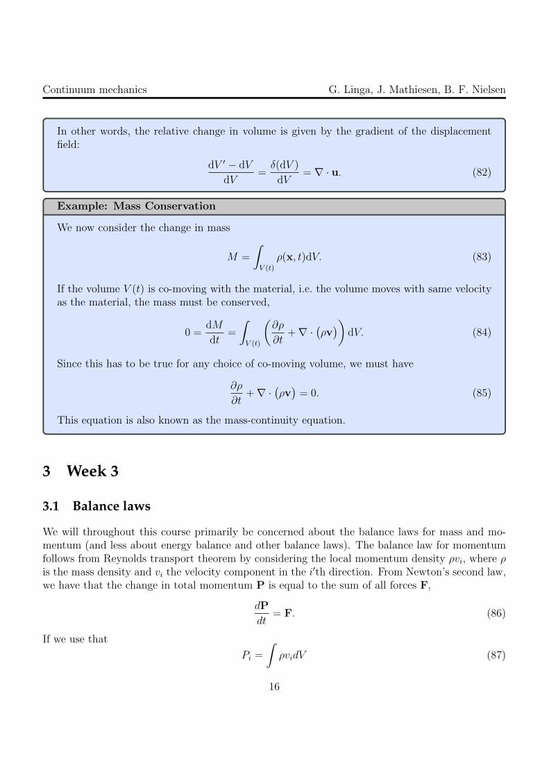
In other words, the relative change in volume is given by the gradient of the displacementfield:

dV ′ − dV

dV=δ(dV )

dV= ∇ · u. (82)

Example: Mass Conservation

We now consider the change in mass

M =

∫V (t)

ρ(x, t)dV. (83)

If the volume V (t) is co-moving with the material, i.e. the volume moves with same velocityas the material, the mass must be conserved,

0 =dM

dt=

∫V (t)

(∂ρ

∂t+∇ ·

(ρv))

dV. (84)

Since this has to be true for any choice of co-moving volume, we must have

∂ρ

∂t+∇ ·

(ρv)

= 0. (85)

This equation is also known as the mass-continuity equation.

3 Week 3

3.1 Balance laws

We will throughout this course primarily be concerned about the balance laws for mass and mo-mentum (and less about energy balance and other balance laws). The balance law for momentumfollows from Reynolds transport theorem by considering the local momentum density ρvi, where ρis the mass density and vi the velocity component in the i′th direction. From Newton’s second law,we have that the change in total momentum P is equal to the sum of all forces F,

dP

dt= F. (86)

If we use that

Pi =

∫ρvidV (87)

16


and use Eq. (28), we achieve from Reynolds transport theorem (assuming that the velocity of therepresentative volume is the co-moving velocity) Eq. (80) that

∂t(ρvi) + ∂j(ρvivj) = fbody,i + ∂jσij. (88)

We now take the derivative of individual terms and arrive at

vi∂tρ+ ρ∂tvi + vi∂j(ρvj) + ρvj∂jvi = fbody,i + ∂jσij, (89)

which we can write on the form

vi[∂tρ+ ∂j(ρvj)] + ρ[∂tvi + vj∂jvi] = fbody,i + ∂jσij, (90)

If we invoke mass balance, the first bracket vanishes and we arrive at the following two fundamentalbalance laws

∂tρ+ ∂j(ρvj) = 0

ρ[∂tvi + vj∂jvi] = fbody,i + ∂jσij (91)

We often use the short-hand notation

D

Dt≡ ∂t + vj∂j

for the so-called co-moving derivative. For example consider the mass conservation, which usingthe co-moving derivative can be written on the form

Dρ

Dt= ρ∂jvj. (92)

This equation states that the temporal change in density inside a co-moving volume (the left-handside) is due to the compression or de-compression of the volume element (right-hand side, see Eq.(82)).

3.2 The temporal elasticity equation

If we insert Hooke’s law, σij = 2µuij + λδijukk, in the momentum balance law Eq. (91), and notethat velocity field follows from the displacement field v = ∂tu, we arrive at

ρ[∂2t ui + vj∂jvi] = fbody,i + µ∂2

kkui + (µ+ λ)∂i∂kuk (93)

Here, we shall consider only small deformations and small amplitude elastic waves, such that theadvection term in the equation can be neglected. We therefore have that

ρ∂2t ui = fbody,i + µ∂2

kkui + (µ+ λ)∂i∂kuk (94)

17


In vector notation the equation has the form

ρ∂2t u = fbody + µ∇2u + (µ+ λ)∇(∇ · u). (95)

If we now use the vector identify

∇×∇× u = ∇(∇ · u)−∇2u (96)

We can write Eq. (95) as

ρ∂2t u = fbody − µ∇×∇× u + (2µ+ λ)∇(∇ · u). (97)

Helmholtz decomposition

Any sufficiently smooth vector field, u can be decomposed in an irrotational (curl-free), uL,and a solonoidal (divergence free) field, uT ,

u = −∇ϕ+∇×Ψ = uL + uT (98)

If we decompose in irrotational and divergence free fields and neglect body forces, we can write Eq.(100) as two seperate equations

ρ∂2t uL = (2µ+ λ)∇2uL. (99)

andρ∂2

TuT = µ∇2uT . (100)

4 Week 4

4.1 Ideal and nearly ideal flow

This week, we will consider inviscid fluids, i.e. fluids where the viscosity is equal to zero. As usual,we start from the mass and momentum balance equations. In addition, we assume that the onlycontribution to the stress tensor comes from a pressure field. In that case, we can write

σij = −pδij (101)

If we insert the stress tensor in the momentum balance law, we arrive at the Euler equation forfluid flow accompanied by mass balance,

ρ(∂t + vj∂j)vi = f bodyi − ∂ip∂tρ+ ∂j(ρvj) = 0 (102)

18


In the incompressible case, we replace the mass balance equation with ∂jvj = 0. There is an inherentsymmetry in the Euler equation, which becomes apparent after some rewriting. We therefore firstdefine the vorticity of the flow

ω ≡ ∇× v (103)

We now use the identity

v × ω =1

2∇v2 − (v · ∇)v (104)

We insert this identify in the Euler equation and assume that the body forces are conservative andcan be written on the form f body = −ρ∇Φ. We now have

∂tv − v × ω = −∇(

1

2v2 +

p

ρ+ Φ

)(105)

For a steady-state (meaning ∂tv = 0) and irrotational flow (the vorticity is zero), we have Bernoulli’slaw

∇(

1

2v2 +

p

ρ+ Φ

)= 0. (106)

By integrating once, we see that the quantity

H ≡ 1

2v2 +

p

ρ+ Φ (107)

is conserved when following a small fluid volume.

4.2 Potential flow

Consider an irrotational and incompressible flow, i.e.

∇× v = 0, and ∇ · v = 0. (108)

If this case, the flow field is determined by the gradient of a scalar field, which by the incompress-ibility satisfies the Laplace equation

v = −∇ψ, and ∇ · v = −∇2ψ = 0 (109)

Two-dimensional potential flow over a half-cylinder

Potential problems in two-dimensions are often conveniently solved in the complex plane. Forexample, consider a cut of a half-cylinder, which becomes a circle, in the upper complex plane witha coordinate w = r + is (where u and v are real numbers). The outside of the circle is mapped tothe full upper plane by a transformation (check!)

z = g(w) = w + 1/w (110)

19


z=g(w)−−−−−→

In the coordinate w, we can write the Laplace equation

∇2ψ = (∂2r + ∂2

s )ψ = (∂r + i∂s)(∂r − i∂s)ψ = 4∂w∂wψ (111)

Similarly, we can write the Laplace equation in the plane z without the circle, i.e. we just solvefor a parallel flow to the x-axis. We call the potential in the full plane for φ. We can calculate thispotential either by using complex or real variables. Here we use the complex variables (the realvariable case can be seen in the book). We now have

4∂z∂zφ = 0,

which implies thatφ(z, z) = h1(z) + h2(z),

where h1 and h2 are some functions which must satisfy the boundary conditions. For an undisturbedideal flow parallel to the x-axis, we have that v = v0ex = −∇φ or similarly in the complex variables−2∂zφ = v0. We therefore have that

h′2(z) = v0/2. (112)

Integrating once, we obtain the complex potential

φ(z, z) = v0z/2 + α, (113)

where α is some constant. Due to the conformal invariance of the Laplace operator φ(w, w) =φ(z, z), the potential for the flow around the disc is ”simply” given by

ψ(w, w) = φ

(g(w), g(w)

)= v0g(w)/2 + α. (114)

From the potential, we now obtain the velocity

v = 2∂wψ(w, w)

= v0∂wg(w)

= v0∂w(w + 1/w)

= v0(1− 1/w2) (115)

20


If we neglect gravity, we obtain from Bernoulli’s law that

const =p∞

ρ+

1

2|v|2 =

p∞

ρ+

1

2v2

0

[1− 2Re

(1

w2

)+

1

|w|4

](116)

If we next set w = reiθ and assume that the pressure at infinity is p∞, we get

p∞

ρ+

1

2v2

0 =p

ρ+

1

2v2

0

[1−

(4 cos2(θ)− 2

r2

)+

1

r4

](117)

5 Week 5

From the inviscid flows, we now turn to dissipative flows. Following the same arguments leading toHooke’s law Eq. (37), viscous forces arise due to gradient in the flow field, or due to compression/de-compression. Fluids homogeneous, isotropic and linear (Newtonian) in the gradient of the velocityfield has a stress tensor on the form (including an additional pressure term)

σij = −pδij + η(∂ivj + ∂jvi) + λ(∂kvk)δij (118)

If we insert this expression in the momentum balance equation, we arrive at the Navier-Stokesequations

ρ(∂t + vj∂j)vi = f bodyi − ∂ip+ η∂2j vi + (η + λ)∂i∂kvk.

Note the similarity with the elasticity equation. If the flow is incompressible, the last term vanishesin the equation, and we have the incompressible Navier-Stokes eqauation.

5.1 Solutions to Stokes’ First and Second Problem

−2 −1 1 2

1

2

V = vx(y, t)ex

vx(0, t) = U0 cos(ωt)x

y

21


We consider a shear flow parallel to the x-z plane, which only depends on the y coordinate, v =vx(y, t)ex. In this case ∇ · v = ∂xvx(y, t) = 0. We further assume that the pressure gradient in thesystem is zero. The flow is driven by an oscillatory motion U0 cos(ωt)ex of the x-z plane in the xdirection for y = 0, i.e. we have the boundary condition for the flow velocity.

Boundary conditions

vx(0, t) = U0 cos(ωt)vx(y, 0) = 0, for y > 0

vx(y, t)y→∞→ 0

(119)

The Navier-Stokes equation reduces in this case to the diffusion equation along the y-axis

∂tvx(y, t) = ν∂2yvx(y, t). (120)

If we apply the Laplace transform with regard to time, we get

svx(y, s)− vx(y, 0)− ν∂2y vx(y, s) = 0. (121)

If we use that initially the fluid is at rest everywhere in the system, vx(y, 0) = 0, we get the simplesecond order differential equation

0 =( sν− ∂2

y

)vx(y, s) =

(√s

ν+ ∂y

)(√s

ν− ∂y

)vx(y, s). (122)

The general solution is

vx(y, s) = A(s)e−√

sνy +B(s)e

√sνy, (123)

where A(s) and B(s) are functions depending on s. We see that the second term is not compatiblewith the boundary condition vx → 0 for y →∞ and therefore set B(s) = 0.

We find the function A(s) from the boundary condition vx(0, t) = U0 cos(ωt), by using Eq. (123)

vx(0, s) = A(s), (124)

which again is

vx(0, s) =

∫ ∞0

U0 cos(ωt)e−stdt =U0s

s2 + ω2. (125)

The complete solution to Stokes’ problems is therefore in the Laplace transformed time

vx(0, s) =U0s

s2 + ω2e−√

sνy. (126)

Now in order to get the solution in the real time variable, we have to apply the inverse Laplacetransform. Things get more easy though, by writing the solution, Eq. (126), as a product of thetwo terms g1(s) = U0s/(s

2 + ω2) and g2(s) = exp(−√s/νy), i.e.

vx(y, s) = g1(s)g2(y, s) (127)

22


If we now use the convolution theorem for the Laplace transform, we get

L−1 [g1(s)g2(y, s)] =

∫ t

0

g1(t− τ)g2(τ)dτ, (128)

where g1 and g2 are the inverse Laplace transformations of g1 and g2, respectively. Note that thevariable y has no influence on the transform. The inverse transform of g1 follows directly fromEq. (125) and is U0 cos(ωt). The inverse transform of g2 is slightly more difficult to compute,

L−1 [g2(y, s)] =1

2πi

∫ λ+i∞

λ−i∞e−√

sνyestds =

ν

2πiy2

∫ λ+i∞

λ−i∞e−√se

νty2sds. (129)

Re

Im

Γε

Γ1Γ2

Γ3

Γ4

Γ5

Figure 3: Integration path

After the second equality we have redefined the integration variables using that y and ν are always positive. The problem in performingthe inverse Laplace transform is that the integrand has a branch cutdue to the square root in the exponent of the first exponential. Wetherefore have to be somewhat careful in choosing the contour alongwhich we perform the integration. We choose the negative real axisas the branch cut and let the argument of the complex numbers runfrom −π to π. We choose an integration path avoiding the branch cutas shown in Fig. 3. We note that as usual for t > 0 the integrationalong the path elements Γ2 and Γ5 vanish, we therefore have that the

inverse Laplace transform can be written along the remaining path elements

0 =ν

2πiy2

∫Γ1+Γ3+Γ4

e−√se

νty2sds. (130)

The combined integral vanishes since no poles exist inside the integration path. If we for simplicitydefine t = νt/y2, we can write∫

Γ1

e−√setsds = −

∫Γ3

e−√setsds−

∫Γ4

e−√setsds

= −eiπ∫ 0

∞e−√r exp(iπ)er exp(iπ)tdr − e−iπ

∫ ∞0

e−√r exp(−iπ)er exp(−iπ)tdr

= −∫ ∞

0

e−i√re−rtdr +

∫ ∞0

ei√re−rtdr

= −2

∫ ∞0

e−iue−u2 tudu+ 2

∫ ∞0

eiue−u2 tudu

= 2

∫ ∞0

(eiu − e−iu

)ue−u

2 tdu

=

∫ ∞−∞

(eiu − e−iu

)ue−u

2 tdu

= 2iIm

[∫ ∞−∞

eiuue−u2 tdu

], (131)

23


where we along the way have made the substitution r = u2 and used the symmetry of the integrandto expand the integration to the whole real axis. We have further taken the imaginary part of thecomplex exponential outside, noting that the exponential involving u2 is real. We can now completethe square, perform the Gaussian-like integral and arrive at the result

ν

2πiy2

∫Γ1

e−√setsds =

ν

πy2Im

[∫ ∞−∞

eiuue−u2 tdu

]=

ν√4πy2t3/2

e−1/(4t) =y√

4πνt3/2e−

y2

4νt (132)

Coming back to Eq. (128), we arrive at the final solution in real space, which has the form

Vx(y, t) = L−1 [g1(s)g2(y, s)] =U0y√4πν

∫ t

0

cos[ω(t− τ)]τ−3/2e−y2

4ντ dτ. (133)

We now have solutions to the two Stokes problems, which corresponds to the cases where eitherthe bottom plate at y = 0 moves at steady speed U0 or oscillates with a frequency ω. Stokes’first problem, the steady motion of the plate, is solved by letting ω = 0 in Eq. (133) and then byperforming the integration,

Vx(y, t) =U0y√4πν

∫ t

0

τ−3/2e−y2

4ντ dτ = erfc

(y

2√νt

), (134)

where erfc denotes the complementary error function. Stokes second problem corresponds to thesteady state oscillation of the bottom plate. The steady state solution is found by letting timeapproach infinity, i.e. let the system evolve long enough that any transient dies out.

Vx(y, t) =U0y√4πν

∫ t

0


4ντ dτ

=U0y√4πν

[∫ ∞0


4ντ dτ −∫ ∞t


4ντ dτ

].

t1≈ U0y√

4πν

∫ ∞0


4ντ dτ

= e−√

ω2νy cos

(ωt−

√ω

2νy

)(135)

6 Week 6

6.1 Stokes flow

In this section, we consider the numerical computation of steady viscous flow in various 2D geomet-ries. We briefly present some background on the finite element method and the FEniCS framework.

24


The section contains three exercises, which are given with increasing difficulty: (1) Laminar pipeflow, (2) force calculation from flow around objects, and (3) lid-driven cavity flow.

Incompressible flow is in general described by the Navier–Stokes equations,

ρ

(∂u

∂t+ (u ·∇)u

)− η∇2u = f −∇p, (136a)

∇ · u = 0, (136b)

where u(x, t) is the velocity field, f(x, t) a body force, ν the kinematic viscosity, and p(x, t) thepressure field.

In many settings the inertial forces are small compared to viscous forces, i.e. the Reynolds numberRe = |u|`/ν 1, where ` is a characteristic length scale of the flow. In this case, eq. (136a) reducesto the time-independent equation2

η∇2u = ∇p− f . (137)

If we further neglect body forces and rescale p→ ηp, we get the equation system

∇2u = ∇p, (138a)

∇2p = 0, (138b)

where eq. (138b) is found by taking the gradient of eq. (138a) and using the incompressibilitycondition eq. (136b).

The system of eqs. (138a) and (138b) are in a domain x ∈ Ω. For simplicity, we will assumeprescribed velocity boundary conditions,

u(x) = u0(x) for x ∈ ∂Ωu, (139)

and prescribed pressure boundary conditions (normal stress),

p(x) = p0(x) for x ∈ ∂Ωp, (140)

where ∂Ω = ∂Ωu ∪ ∂Ωp is the boundary of Ω.

6.2 Finite Element Method

The finite element method (FEM) is an efficient method for solving partial differential equations(PDEs) in complex geometries. Basically, it consists in approximating the solution to a PDE ratherthan approximating the equation itself (as you do with finite difference methods and finite volumemethods). This is obtained by employing calculus of variations. We will not present the FEM

2On very short time scales, however, the time-derivative term may be important.

25


theory in detail here, just a direct explanation of how our program will work. For a thoroughintroduction, see e.g. [1, 5].

The quick and dirty recipe of FEM is the following: The domain is discretized by dividing it intomany subdomains, called elements. In our case, the elements are triangles. On each element, weapproximate the solution by linear combinations of basis functions defined on each element. Theelement-wise equations defining the coefficients in these linear combinations are assembled for theentire system, yielding a (large, and often sparse) set of algebraic equations to be solved.

In order to use FEM to solve our equations, we must formulate the problem in a weak (variational)form. The basis functions belong to the function spaces V (velocity space) and P (pressure space)

By multiplying our equations (unknowns = trial functions (u, p)) by the test functions (v, q) andsuccessively integrating by parts, we may obtain the following (weak) problem formulation:

Weak formulation: Find (u, p) ∈ W such that

a((u, p), (v, q)) = L((v, q)) for all (v, q) ∈ W, (141a)

and u = u0 on ∂Ω, (141b)

where W = V × P is a mixed function space, and

a((u, p), (v, q)) =

∫Ω

(∇u : ∇v − p∇ · v + q∇ · u) dV, (141c)

L((v, p)) = −∫∂Ωp

p0n · vdS. (141d)

This problem formulation is all we need. Now, to avoid most of the technicalities of FEM (actuallyconstructing the basis functions, solving the integral equations on the element level, assembling thesystem matrix, and enforcing the boundary conditions, . . . ) and get straight to the physics, we usethe FEniCS framework.

6.3 FEniCS/DOLFIN

FEniCS is a collection of software for automated solution of PDEs using FEM [7]. The componentof FEniCS we will use to communicate with the FEniCS engine via Python is called DOLFIN [8].Some of the functionality we will use is

• Making a simple mesh

• Setting up subspaces and basis functions

• Applying boundary conditions

• Solving the system

26


• Visualizing the solution

The bottom line is, all we need to do is to supply the variational form and boundary conditionsand the order of the elements (i.e. the polynomial degree of the basis functions)—FEniCS does therest (and it’s quite fast!).

Tip: If you want to get really dirty with FEniCS, you should consider following their excellenttuturial [6].

6.4 Getting started with FEniCS

If you are a student at University of Copenhagen, you should already have access to FEniCS throughERDA using your University of Copenhagen login on http://erda.dk. If it is the first time youlog in, you may have to go through a few steps to activate your user. Once you are logged intoERDA you have the possibility to start python through a jupyter notebook by 1) clicking ”jupyter”in menu, 2) ”start DAG” and 3) start a server with ”Finite element notebook using FEniCS”. Ifyou prefer to have FEniCS installed locally on your own computer (only recommended if you plentyof time), you can follow the instructions on http://fenicsproject.org/download/. We wouldrecommend using either Docker or Ubuntu.

In the following, you will be asked to run simulations for different input parameters. If you are anadvanced Python programmer, you may want to make automated scripts, and systematically storethe input and output values to a data file running python in a terminal. However, here, we keepthe plotting to the minimal possible within a jupyter notebook. We will also for simplicity restrictour attention to flow in two dimensions.

In general, we suggest that you break your program down in small units (functions) which you cantest individually. If the components themselves work, for any input, it is likely that the whole thingwill work.

6.4.1 Pipe flow

p

pleft pright

uwall = 0

Figure 4: Pipe flow setup.

The first case concerns simulation of pipe flow. In this case we will go step-by-step through anexample program. We shall consider a pipe of diameter d = 4 and length l = 10, as shown in fig. 4.

27

http://erda.dk

http://fenicsproject.org/download/


On the left side, we prescribe the pressure p(0, y) = 1 and on the right p(l, y) = 0. Along the pipewalls we use the no-slip condition u(x, 0) = u(x,D) = 0.

Load DOLFIN: First, we need to load all the capabilities of FEniCS using the Python moduleDOLFIN, and the numerical tools package Numpy. This can be done using

from dolfin import *

import numpy as np

where we have for convenience adopted the entire dolfin namespace.

Domain and mesh: We now have to define and discretize our domain. To create the domain,we can use the function RectangleMesh(p0, p1, nx, ny, diagonal="right") which draws anx×ny rectangle between the points p0 and p1.

This can e.g. be done as

# Define domain and discretization

delta = 0.5

length = 10.0

diameter = 4.0

# Create mesh

p0 = Point(np.array([0.0, 0.0]))

p1 = Point(np.array([length, diameter]))

nx = int(length/delta)

ny = int(diameter/delta)

mesh = RectangleMesh(p0, p1, nx, ny)

You can interactively visualize the mesh using

plot(mesh, title="Mesh")

interactive()

Mark the boundary: In order to apply boundary conditions, we must mark the different parts ofthe boundary correctly. We may first define some labels,

# Making a mark dictionary

# Note: the values should be UNIQUE identifiers.

mark = "generic": 0,

"wall": 1,

"left": 2,

"right": 3

28


Now we define a function marking the subdomains of the mesh. We first mark the entire domainas “generic”.

subdomains = MeshFunction("size_t", mesh, 1)

subdomains.set_all(mark["generic"])

The subdomain function should be marked with the correct labels on the correct parts of the mesh.Now, we define the Left part of the boundary, which inherits the SubDomain class:

class Left(SubDomain):

def inside(self, x, on_boundary):

return on_boundary and near(x[0], 0)

Here, on boundary is a flag indicating if a node is on the boundary, and near(a, b) is a functionreturning true if a and b are approximately equal (difference below some threshold). Note thatx[0] refers to the first coordinate of x.

♠ Write the classes Right and Wall for the remaining boundaries.

Now we apply the mark defined previously for the boundaries:

left = Left()

left.mark(subdomains, mark["left"])

Now the left boundary has been marked.

♠ Mark the boundaries right and wall as well.

Finally, you can visualize the subdomains mesh function using the command

plot(subdomains, title="Subdomains")

interactive()

♠ Do the boundaries have the correct value according to the mark labels defined above?

Define function spaces: We now move away from the boundary for a little while. We define ourfunction spaces, effectively the set of basis functions on our elements. To avoid stability issues whichcan be a problem for mixed spaces (look up the Babuska–Brezzi condition), we use Taylor–Hoodelements to resolve the problem. This means that we use second-order continuous-Galerkin (CG)basis functions for the velocity and first-order CG for the pressure.

This can be implemented as follows, by first defining the elements and constructing a functionspace from this:

# Define function spaces

V = VectorElement("CG", triangle, 2)

P = FiniteElement("CG", triangle, 1)

W = FunctionSpace(mesh, V*P)

29


Here, W is the mixed space.

Define variational problem: We now define trial and test functions living in the space W:

# Define variational problem

(u, p) = TrialFunctions(W)

(v, q) = TestFunctions(W)

We also define measures for our integration (matrix assembly). We supply subdomains to dividethe domain according to which mark it has (see below).

dx = Measure("dx", domain=mesh, subdomain_data=subdomains) # Volume integration

ds = Measure("ds", domain=mesh, subdomain_data=subdomains) # Surface integration

To assemble the surface integral in the variational form, we need the surface normal, the inlet/outletpressures, and a (dummy) body force:

# Surface normal

n = FacetNormal(mesh)

# Pressures. First define the numbers (for later use):

p_left = 1.0

p_right = 0.0

# ...and then the DOLFIN constants:

pressure_left = Constant(p_left)

pressure_right = Constant(p_right)

# Body force:

force = Constant((0.0, 0.0))

Finally, we are ready to feed DOLFIN the variational form, cf. eqs. (141a) to (141d):

a = inner(grad(u), grad(v))*dx - p*div(v)*dx + q*div(u)*dx

L = inner(force, v) * dx \

- pressure_left * inner(n, v) * ds(mark["left"]) \

- pressure_right * inner(n, v) * ds(mark["right"])

Apply (Dirichlet) boundary conditions: We now return to the boundary. The no-slip (zerovelocity) boundary condition can be defined as:

noslip = Constant((0.0, 0.0))

bc_wall = DirichletBC(W.sub(0), noslip, subdomains, mark["wall"])

Here, W.sub(0) refers to the first subspace of W, namely V. Similarly, W.sub(1) refers to P.

30


♠ Implement also the pressure boundary conditions bc left and bc right, using, respectively,pressure left and pressure right. Remember that this must be applied to the pressuresubspace using W.sub(1).

Finally, we collect the boundary conditions into one vector:

bcs = [bc_wall, bc_left, bc_right]

Solve variational problem: The problem is now fully specified, and all that remains is to solveit. We define the temporary solution vector w (corresponding to the mixed space W), and solve thevariational problem with the supplied Dirichlet BCs bcs using the function solve(problem, w,

bcs). If problem is of the form a == L, as below, DOLFIN automatically deduces that it is alinear problem.

# Compute solution

w = Function(W)

solve(a == L, w, bcs)

Finally, we split the solution vector w into its velocity and pressure parts:

# Split using deep copy

(u, p) = w.split(True)

This should give you the solution for velocity and pressure, respectively through u and p.

Visualize the solution: The straightforward plotting tool is easy to use:

# Plot solution

plot(u, title="Velocity")

plot(p, title="Pressure")

interactive()

You might want to visualize the speed |u|. It is therefore useful to implement the functionmagnitude:

# Magnitude function

def magnitude(vec):

return sqrt(vec**2)

Then you can plot the speed by:

plot(magnitude(u), "Speed")

Tip: For more sophisticated interactive plotting, you can use ParaView[4]. Export the solutionusing the following commands:

31


# Save solution in VTK format

ufile = File("velocity.pvd")

ufile << u

pfile = File("pressure.pvd")

pfile << p

Now you can open the .pvd-files using ParaView.

Assess the solution: You are now asked to inspect the solution.

♠ How does the solution for the velocity field u look? What about the pressure p?

♠ Vary and interchange the values of p left and p right. How does the solution change?

♠ How does the numerical solution, for u and p, compare to the analytical solution?

One way of doing this quantitatively is the following: Construct first the analytical solution inthe domain. This is done by constructing an Expression (which evaluates C code in the domain;therefore we have to pass variables in a special way—see code below), and interpolating it onto theV subspace. For both p and u:

# Define coefficient

coeff = (p_left-p_right)/(2*length)

# Define expressions

u_analytic = Expression(("C*x[1]*(2.0*rad - x[1])", "0.0"),

C=coeff, rad=0.5*diameter, degree=2)

p_analytic = Expression("p_l - 2*C*x[0]", p_l=p_left, C=coeff,

degree=1)

# Project onto domains

u_analytic = interpolate(u_analytic, W.sub(0).collapse())

p_analytic = interpolate(p_analytic, W.sub(1).collapse())

Subtract the analytical solution from the original one and take the magnitude:

u_error_local = magnitude(u - u_analytic)

Integrate (assemble) over the whole domain to get the global error:

u_error = assemble(u_error_local*dx)

print "u_error =", u_error

♠ How do the errors in u and p change as you refine the grid (i.e. change delta)?

Normally, we would expect that the error decreases with refined grid according to the order of theelements.

♠ Why may this not happen here? Hint: Look at the polynomial order of the function spacesV and P and of the analytical solution for u and p.

32


The divergence of the velocity field is found by

div_u = div(u)

div_u = project(div_u, W.sub(1).collapse()) # Project on the pressure subspace since it is scalar order 1 (V is 2)

and it should, of course, be zero for infinite numerical precision.

♠ How does the error in ∇ · u change as you refine the grid?

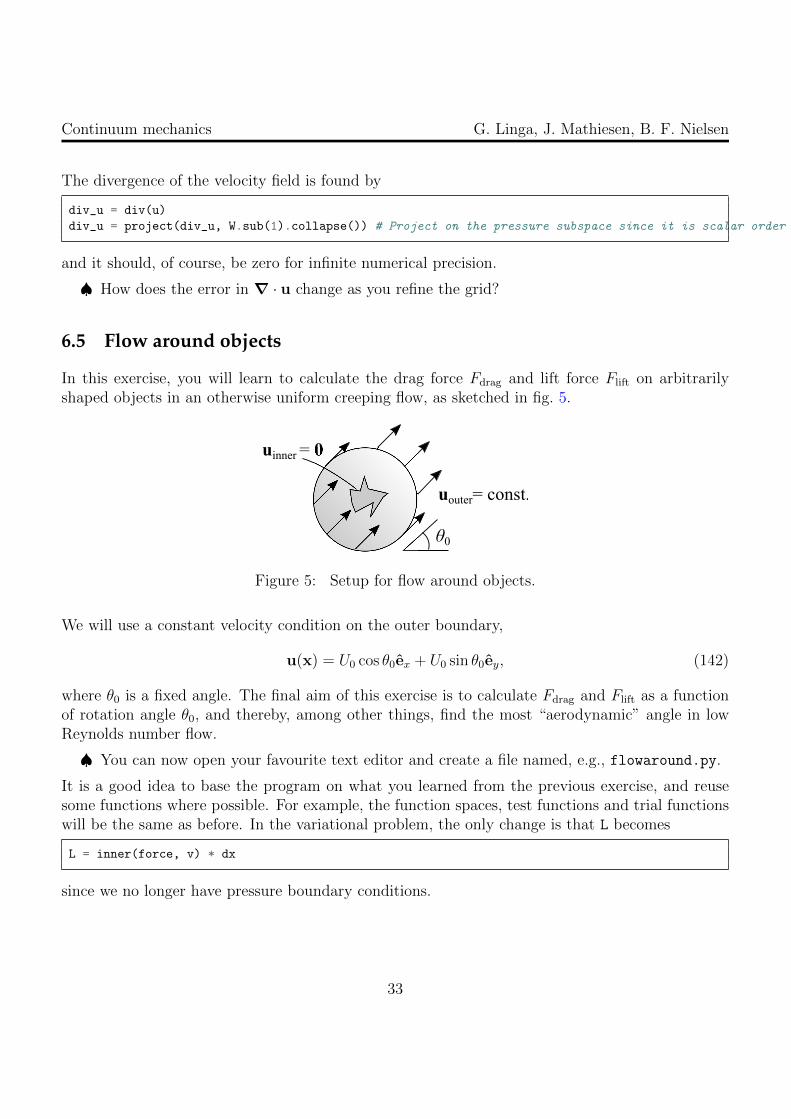
6.5 Flow around objects

In this exercise, you will learn to calculate the drag force Fdrag and lift force Flift on arbitrarilyshaped objects in an otherwise uniform creeping flow, as sketched in fig. 5.

uouter= const.

uinner = 0

θ0

Figure 5: Setup for flow around objects.

We will use a constant velocity condition on the outer boundary,

u(x) = U0 cos θ0ex + U0 sin θ0ey, (142)

where θ0 is a fixed angle. The final aim of this exercise is to calculate Fdrag and Flift as a functionof rotation angle θ0, and thereby, among other things, find the most “aerodynamic” angle in lowReynolds number flow.

♠ You can now open your favourite text editor and create a file named, e.g., flowaround.py.

It is a good idea to base the program on what you learned from the previous exercise, and reusesome functions where possible. For example, the function spaces, test functions and trial functionswill be the same as before. In the variational problem, the only change is that L becomes

L = inner(force, v) * dx

since we no longer have pressure boundary conditions.

33


Meshes: In this case, we will supply you with meshes (or you can make your own, if you preferand are able to).

The following meshes are provided:

• An obstacle-free mesh (http://www.nbi.dk/~mathies/free_2d.xml.gz),

• Circular obstacle (http://www.nbi.dk/~mathies/circle_2d.xml.gz),

• NACA airfoil [2] obstacle (http://www.nbi.dk/~mathies/naca_2d.xml.gz).

Download the mesh files and upload them to your ERDA folder. You can then load the pre-generated mesh by the following command:

mesh = Mesh("free_2d.xml.gz")

Mark the boundary: In this case, we have two boundaries: outer and inner boundary.

♠ Mark the boundary in a similar manner as in the previous exercise, but now with the boundarymark labels "inner boun" and "outer boun".

Hint: The command

rad2 = x[0]**2 + x[1]**2

gives the squared distance from the center, and the flag on boundary yields (as before) True if apoint is on the boundary or False if not. The meshes we provide you with are centered at theorigo. Note: You should not use the name inner on a variable, as this name is reserved for theinner product function in DOLFIN.

♠ Visualize the subdomains function to ensure that the boundary is correctly marked.

Apply (Dirichlet) boundary conditions: Similarly as in the previous exercise, we will applyDirichlet boundary conditions on the velocity field. For prescribed, constant boundary velocity,this can be achieved by the commands:

u_outer_boun = Constant((U_0*cos(theta), U_0*sin(theta)))

bc_outer_boun = DirichletBC(W.sub(0), u_outer_boun, subdomains, mark["outer_boun"])

♠ Implement and apply the (no-slip) inner boundary condition as well.

To have a well-posed problem you need to fix the pressure at one node to some reference value.Take e.g. the node to the left:

bc_p = DirichletBC(W.sub(1), 0, "x[0] < -1.0 + DOLFIN_EPS", "pointwise")

34

http://www.nbi.dk/~mathies/free_2d.xml.gz

http://www.nbi.dk/~mathies/circle_2d.xml.gz

http://www.nbi.dk/~mathies/naca_2d.xml.gz


Analyse the solution: You now have all the information needed to calculate the flow in any ofthese domains.

First, to verify that the solver is working correctly, you can run a simulation using the meshfree 2d.xml.gz, where the domain is free of obstacles.

♠ Does the solution match the (trivial) analytical solution?

Now, we switch to more complex geometries. The following tasks should be done for the meshcircle 2d.xml.gz (flow around a circle) and naca 2d.xml.gz (NACA airfoil).

♠ Visualize the solution for an angle of choice θ0. Where is the pressure and velocity highestand lowest? Why?

The second deviatoric stress invariant, J2, which measures how sheared the liquid is, is given by

J2 =1

2tr(σ2

visc). (143)

Calculation of the viscous stress tensor, total stress tensor and J2 can be implemented as follows:

# Viscous stress

# sym returns the symmetric part of a matrix

stress_visc = 2*sym(grad(u))

# Total stress

stress = -p*Identity(2) + stress_visc

# Second deviatoric (viscous) stress invariant

J_2 = 0.5*tr(stress_visc*stress_visc)

♠ Calculate the viscous and total stress in the fluid, and visualize J2.

Tip: If you want to visualize it in ParaView, you can export the tensor field σ by the followingcommands:

T = TensorFunctionSpace(mesh, "CG", 1) # Order 1, as it is a deriv. of V (order 2)

stress = project(stress, T)

stress_file = File("stress.pvd")

stress_file << stress

We will now calculate the traction on the inner boundary, and decompose it into a drag force anda lift force by using the direction of the imposed flow, n flow. A way to do this is the following,assuming you have already calculated the boundary normal n and the surface measure ds (seeprevious exercise if you haven’t):

# Imposed flow direction:

n_flow = Constant((cos(theta), sin(theta)))

n_flow = project(n_flow, W.sub(0).collapse())

35


# Perpendicular to n_flow:

t_flow = Constant((sin(theta), -cos(theta)))

t_flow = project(t_flow, W.sub(0).collapse())

# Compute traction vector

traction = dot(stress, n)

# Integrate decomposed traction to get total F_drag and F_lift

F_drag = assemble(dot(traction, n_flow) * ds(mark["inner"]))

F_lift = assemble(dot(traction, t_flow) * ds(mark["inner"]))

Now you should be able to calculate the lift force Flift and drag force Fdrag for any imposed flowangle θ0.

♠ Systematically vary the imposed flow angle θ0 ∈ [0, 2π] and plot Flift and Fdrag as functionsof θ0. Locate the extremal points.

♠ Do you recognize the symmetry of the geometry (and the equations) in the plotted graphs?

Extra task for the most ambitious: As you might be aware of, “unbounded” Stokes flowcan not occur in 2D (see Stokes’ paradox, e.g. [3]). This makes our numerical experiments onlyapplicable to confined flows, and our calculated drag coefficients would not converge to a finitevalue as we increased the domain and kept the obstacle size fixed. To add some realism, you aretherefore invited to include the inertia term in your calculations. The necessary information fordoing so is given in the next exercise.

♠ Plot the drag force Fdrag as a function of Re for different angles. How does it change withincreasing Re? It has been proposed that Fdrag ∼ Re−1 for small Re. Can you see this fromyour simulations?

6.6 Lid-driven cavity

You are quickly becoming an expert in FEniCS. We shall now consider one of the classic testcases in computational fluid dynamcs (CFD), namely that of lid-driven cavity flow. We considera square geometry (cavity) with side length l = 1. The left, right and bottom boundaries haveno-slip conditions and the top (lid) is driven with a velocity U0 = 1 in the x direction. This resultsin a circulation in the cavity. The setup is sketched in fig. 6.

♠ Open your favourite text editor and create a file named, e.g., cavity.py.

♠ Create a mesh for the cavity, in the area [0, l] × [0, l]. You can start with discretizationresolution N = 32 (=nx=ny) points along each axis.

♠ Create the classes Wall and Lid to mark the boundary of the cavity.

In this case, we shall explore the effect of including the advection term in the solver, i.e. investigateRe > 0. We will still restrict our scope to seeking steady-state solutions. The equations describing

36


ulid = u0ex

uwall = 0

Figure 6: Setup for lid-driven cavity flow.

the problem are then, disregarding the body force,

ν∇2u− (u ·∇)u = ∇p, (144a)

∇ · u = 0 (144b)

so that the weak form of the problem becomes: Find (u, p) ∈ W such that∫Ω

(ν∇u : ∇v + (u ·∇u) · v − p∇ · v + q∇ · u) dV = 0 for all (v, q) ∈ W. (145)

The non-linear functional F describing the problem can be impemented as

F = inner(grad(u)*u, v)*dx \

+ nu*inner(grad(u), grad(v))*dx \

- p*div(v)*dx \

- q*div(u)*dx

Here, some variables (w, u, p, nu) have to be defined beforehand, by

Reynolds = 1.0 # or any other value

nu = 1./Reynolds

# Solution vectors

w = Function(W)

u, p = (as_vector((w[0], w[1])), w[2])

The inertia term is non-linear, so a standard linear solver will not do in solving this problem. Tooptimally use a non-linear solver, we supply the Jacobian with respect to the (mixed) field w thatwe are solving for. This is implemented as the following:

J = derivative(F, w) # Jacobian

Then the non-linear solver can be invoked:

solve(F == 0, w, bcs, J=J)

37


Here, the solve() function automatically recognizes the form F == 0 as a non-linear problem.Newton’s method is the default non-linear solver, and works well for relatively small meshes. Youcan set the reference pressure BC at the bottom-left-most node by

bc_p = DirichletBC(W.sub(1), 0, "x[0] < DOLFIN_EPS && x[1] < DOLFIN_EPS", "pointwise")

Remember that you have to include bc p in the bcs vector.

♠ Implement the above, along with the described boundary conditions, to solve the steady-stateNavier–Stokes equations for lid-driven cavity flow. Visualize the resulting fields.

The most straightforward way to get the streamlines of the flow field we can place “particles”at random in the domain and passively advect them, i.e. integrate up their velocity. The scripttrace.py we provide you with does this. First, you have to export the mesh and velocity field to.xml.gz format.

u_file = File("u_Re" + str(Reynolds) + "_N" + str(N) + ".xml.gz")

mesh_file = File("mesh.xml.gz")

u_file << u

mesh_file << mesh

Then you can open a new terminal and run the script by:

python trace.py mesh.xml.gz u_Re10_N100.xml.gz trace_Re10_N100.dat -ds 0.005 -S 5 -n 100

This will create a data file trace Re10 N100.dat with the trajectories of 100 tracers, where theintegration step length is 0.005 and total path length is 5. The latter file is structured as blocks(one block per tracer) of space-separated data in the following order: tracer ID, time t, x, y, ux,uy, i.e. you need to plot column 3 and 4. In Gnuplot, this is straightforward:

pl 'cavity_data/trace_Re10_N100.dat' u 3:4 w l

♠ Plot streamlines of the flow for some values of Re < 1000 (changing Re amounts to changingthe viscosity ν). How does the flow change?

Tip: You may have to increase the grid resolution N to achieve convergence.

A Tensor subtleties (covered in week 2)

This section describes some of the subtleties of tensor calculus which are in general very important,but which can be ”brushed under the carpet” in most of this course since we will be discussingsufficiently simple situations. In particular we can usually make do with the somewhat more re-stricted concept of a Cartesian tensor.

38


Contravariant and covariant tensors In a general theory, one will need to distinguish betweentwo separate classes of indices when specifying tensors, namely the contravariant indices and thecovariant ones. Contravariant indices are written as superscripts:

V i (Components of a contravariant rank-1 tensor – a vector. Also called a (1,0) tensor)

Covariant indices, on the other hand, are written as subscripts:

ωi (Components of a covariant rank-1 tensor – a co-vector. Also called a (0,1) tensor)

”Why the need for different types of indices?” you may ask.Well, the short answer is ”Because |V 〉 and 〈V | are not the same!”.The difference is probably most directly appreciated via an example. Consider the following twoquantities

V i :=dxi

dt= vi, (146)

ωi :=∂f

∂xi, (147)

where f is some smooth function of the coordinates xi and vi is a velocity vector of some particle.What differs between these two quantities are their transformation properties – in other wordshow they behave under change of coordinates.A change of coordinates is a set of new coordinates given as functions of the old coordinates:

xi → xi = xi(x) (148)

One example could be a rotation around the z axis by an angle α:

xi → xi = Rijx

j, (149)

where Rij is the following rotation matrix:

Rij =

cos(α) − sin(α) 0sin(α) cos(α) 0

0 0 1

(150)

The vector V i changes in the following way under such a change of coordinates:

V i =dxi

dt=∂xi

∂xjdxj

dt=∂xi

∂xjV j = Ri

jVj. (151)

Whereas ωi changes in the opposite manner ! To see this, we simply use the chain rule:

ωi =∂f

∂xi=∂xj

∂xi∂f

∂xj= (R−1) ji ωj. (152)

39


For a rotation matrix it holds that R−1 = RT so that

ωi = (RT ) ji ωj. (153)

This last part was of course particular to rotations, but the more general take-home message isthat contravariant and covariant tensors transform oppositely:

V i =∂xi

∂xjV j,

ωi =∂xj

∂xiωj. (154)

There is a simple physical argument for why it has to be so. Imagine a simple transformationcorresponding to a change of units. If you decide to use a 10cm measuring rod instead of a meterstick, the components of a vector such as V i become ten times as large, numerically. On the otherhand, a gradient such as ωi becomes ten times smaller, numerically, since it represents how fast thefunction f changes as you move one unit in some direction.In certain situations we can neglect to distinguish between covariant and contravariant indices.More on this later. First we shall introduce a special tensor, the metric.

The metric When working in ordinary Euclidean space or on flat surfaces, we’re used to computingdistances by using Pythagoras:

ds2 = dx2 + dy2, (155)

where ds2 is the length of the shortest path from points (x, y) to (x+ dx, y + dy). Note that we’respecializing to 2 dimensions here, to keep things simple. Using the Kronecker delta, δij, this canalso be written as

ds2 = dxiδijdxj, (156)

where xi is the vector of coordinates (x and y in this case). Recall that the Einstein summationconvention is in force, so the above represents a sum over i as well as j.However, as soon as we’re working on a curved surface, such as the surface of a sphere, Pythagorasdoesn’t hold anymore. On a sphere we would usually prefer to use the azimuthal and polar angles(φ, θ) to describe things. In this case the (infinitesimal) distance should be computed as

ds2 = R2dθ2 +R2 sin2(θ)dφ2. (157)

40


Exercise

Show that an infinitesimal line element between points (φ, θ) and (φ+dφ, θ+dθ) on a sphereof radius R is given by (157).

We wish to mimic what we did above with the Kronecker delta. In other words, we wish to find atensor gij such that the distances can be computed as

ds2 = dxigijdxj, (158)

where xi are our chosen coordinates, namely (φ, θ). In that case we must choose

gθθ = R2, gφφ = R2 sin2(θ), gθφ = gφθ = 0. (159)

In matrix notation this reads

gij =

[R2 sin2(θ) 0

0 R2

](160)

This is the metric tensor of a sphere. It essentially contains all the geometrical information aboutthe space and – concretely – allows us to compute distances in the space.Note that this tensor could also have been obtained from it’s Euclidean counterpart, which is δij,as described above. To do this, we just need to use the tensor transformation law. We saw in (154)how vectors and co-vectors transform. To get the transformation law for the tensor gij you justtransform each of the indices according to the same law!In other words:

gij =∂xk

∂xi∂xl

∂xjgkl. (161)

In going from Cartesian to spherical coordinates, the ’old’ metric is δij, so we write

gij =∂xk

∂xi∂xl

∂xjδkl. (162)

The coordinates are of course related by

x = R cos(φ) sin(θ),

y = R sin(φ) sin(θ),

z = R cos(θ).

41


Thus we find the relations

∂x

∂φ= −R sin(φ) sin(θ),

∂x

∂θ= R cos(φ) cos(θ),

∂y

∂φ= R cos(φ) sin(θ),

∂y

∂θ= R sin(φ) cos(θ),

∂z

∂φ= 0,

∂z

∂θ= −R cos(θ).

So to compute a component of the spherical metric, we would simply write

gφφ =∂xk

∂φ

∂xl

∂φδkl =

(∂x

∂φ

)2

+

(∂y

∂φ

)2

+

(∂z

∂φ

)2

= R2(sin2(θ) cos2(φ) + sin2(θ) sin2(φ) + 0

)= R2 sin2(θ). (163)

We see that the result fits with what we found in (160).

The metric and the strain tensor Recall that in 1.4 we found the Euler Strain tensor by con-sidering a deformation given by x = f(X) where X i are the reference coordinates and xi are thedeformed coordinates.There we found the expression

dxidxi − dXidXi =

(δk` −

∂f−1i

∂x`

∂f−1i

∂xk

)dx`dxk (164)

We see that the quantity in the brackets is just the difference between the undeformed and deformedmetrics! So the Euler strain tensor just tells you by how much the metric has changed.

References

[1] Wikipedia: Finite element method. https://en.wikipedia.org/wiki/Finite_element_

method, 2016. Online; accessed 13 March 2016.

[2] Wikipedia: NACA airfoil. https://en.wikipedia.org/wiki/NACA_airfoil, 2016. Online;accessed 13 March 2016.

42

https://en.wikipedia.org/wiki/Finite_element_method

https://en.wikipedia.org/wiki/Finite_element_method

https://en.wikipedia.org/wiki/NACA_airfoil


[3] Wikipedia: Stokes’ paradox. https://en.wikipedia.org/wiki/Stokes%27_paradox, 2016.Online; accessed 13 March 2016.

[4] Utkarsh Ayachit. The ParaView guide: A parallel visualization application. Kitware, Inc.,2015.

[5] Young W. Kwon and Hyochoong Bang. The finite element method using MATLAB. CRC press,2000.

[6] Hans Petter Langtangen and Anders Logg. Solving PDEs in Minutes - The FEniCS TutorialVolume I. https://fenicsproject.org/pub/tutorial/html/ftut1.html, 2016. Online; ac-cessed 13 March 2016.

[7] Anders Logg, Kent-Andre Mardal, and Garth Wells. Automated solution of differential equationsby the finite element method: The FEniCS book, volume 84. Springer Science & Business Media,2012.

[8] Anders Logg, Garth N Wells, and Johan Hake. DOLFIN: A C++/Python finite element library.In Automated Solution of Differential Equations by the Finite Element Method, pages 173–225.Springer, 2012.

43

https://en.wikipedia.org/wiki/Stokes%27_paradox

https://fenicsproject.org/pub/tutorial/html/ftut1.html

Documents

Short Comments on Continuum Mechanics: Theory and Computation