Embed Size (px)
DESCRIPTION
BY George Backus 1997
Citation preview

Continuum Mechanics
George Backus
Insitute for Geophysics and Planetary Physics
University of California� San Diego
S Samizdat
Press

Published by the Samizdat Press
Center for Wave Phenomena
Department of Geophysics
Colorado School of Mines
Golden� Colorado �����
and
New England Research
�� Olcott Drive
White River Junction� Vermont �����
c�Samizdat Press� ����
Samizdat Press publications are available via FTP
from landau�mines�edu or �����������
Or via the WWW from http���landau�mines�edu� samizdat
Permission is given to freely copy these documents�
Contents
Dictionary D��
Five Prerequisite Proofs PP��
I Tensors over Euclidean Vector Spaces �
� Multilinear Mappings �
��� De�nition of multilinear mappings � � � � � � � � � � � � � � � � � � � � � �
�� Examples of multilinear mappings � � � � � � � � � � � � � � � � � � � � � � �
�� Elementary properties of multilinear mappings � � � � � � � � � � � � � � � �
��� Permuting a multilinear mapping � � � � � � � � � � � � � � � � � � � � � � �
� De�nition of Tensors over Euclidean Vector Spaces ��
� Alternating Tensors� Determinants� Orientation� and n�dimensional Right�
handedness ��
�� Structure of �nV � � � � � � � � � � � � � � � � � � � � � � � � � � � � � � � �
� Determinants of linear operators � � � � � � � � � � � � � � � � � � � � � � � ��
� Orientation � � � � � � � � � � � � � � � � � � � � � � � � � � � � � � � � � � �
� Tensor Products ��
��� De�nition of a tensor product � � � � � � � � � � � � � � � � � � � � � � � � �
�� Properties of tensor products � � � � � � � � � � � � � � � � � � � � � � � � � �
i

ii CONTENTS
�� Polyads � � � � � � � � � � � � � � � � � � � � � � � � � � � � � � � � � � � � �
� Polyad Bases and Tensor Components ��
��� Polyad bases � � � � � � � � � � � � � � � � � � � � � � � � � � � � � � � � � � �
�� Components of a tensor relative to a basis sequence� De�nition � � � � � �
�� Changing bases � � � � � � � � � � � � � � � � � � � � � � � � � � � � � � � � �
��� Properties of component arrays � � � � � � � � � � � � � � � � � � � � � � � �
��� Symmetries of component arrays � � � � � � � � � � � � � � � � � � � � � � �
��� Examples of component arrays � � � � � � � � � � � � � � � � � � � � � � � � �
� The Lifting Theorem ��
Generalized Dot Products �
��� Motivation and de�nition � � � � � � � � � � � � � � � � � � � � � � � � � � � ��
�� Components of P hqiR � � � � � � � � � � � � � � � � � � � � � � � � � � � � ��
�� Properties of the generalized dot product � � � � � � � � � � � � � � � � � � ��
��� Applications of the generalized dot product � � � � � � � � � � � � � � � � � ��
How to Rotate Tensors �and why� �
��� Tensor products of linear mappings � � � � � � � � � � � � � � � � � � � � � ��
�� Applying rotations and re�ections to tensors � � � � � � � � � � � � � � � � ��
�� Physical applications � � � � � � � � � � � � � � � � � � � � � � � � � � � � � �
��� Invariance groups � � � � � � � � � � � � � � � � � � � � � � � � � � � � � � � ��
��� Isotropic and skew isotropic tensors � � � � � � � � � � � � � � � � � � � � � ��
Di�erential Calculus of Tensors
��� Limits in Euclidean vector spaces � � � � � � � � � � � � � � � � � � � � � � ��
�� Gradients� De�nition and simple properties � � � � � � � � � � � � � � � � � ��
�� Components of gradients � � � � � � � � � � � � � � � � � � � � � � � � � � � ��
��� Gradients of dot products � � � � � � � � � � � � � � � � � � � � � � � � � � ���
��� Curvilinear coordinates � � � � � � � � � � � � � � � � � � � � � � � � � � � � ���

CONTENTS iii
��� Multiple gradients and Taylor�s formula � � � � � � � � � � � � � � � � � � � ��
��� Di�erential identities � � � � � � � � � � � � � � � � � � � � � � � � � � � � � ���
�� Integral Calculus of Tensors ��
���� De�nition of the Integral � � � � � � � � � � � � � � � � � � � � � � � � � � � ���
������ Mass distributions or measures � � � � � � � � � � � � � � � � � � � ���
����� Integrals � � � � � � � � � � � � � � � � � � � � � � � � � � � � � � � � ��
��� Integrals in terms of components � � � � � � � � � � � � � � � � � � � � � � � �
�� Integral Identities ��
���� Linear mapping of integrals � � � � � � � � � � � � � � � � � � � � � � � � � � ��
��� Line integral of a gradient � � � � � � � � � � � � � � � � � � � � � � � � � � ��
��� Gauss�s theorem � � � � � � � � � � � � � � � � � � � � � � � � � � � � � � � � ��
���� Stokes�s theorem � � � � � � � � � � � � � � � � � � � � � � � � � � � � � � � ��
���� Vanishing integral theorem � � � � � � � � � � � � � � � � � � � � � � � � � � �
���� Time derivative of an integral over a moving volume � � � � � � � � � � � � ��
���� Change of variables of integration � � � � � � � � � � � � � � � � � � � � � � ��
II Elementary Continuum Mechanics ���
�� Eulerian and Lagrangian Descriptions of a Continuum ���
��� Discrete systems � � � � � � � � � � � � � � � � � � � � � � � � � � � � � � � � ���
�� Continua � � � � � � � � � � � � � � � � � � � � � � � � � � � � � � � � � � � � ��
�� Physical quantities � � � � � � � � � � � � � � � � � � � � � � � � � � � � � � ���
��� Derivatives of physical quantities � � � � � � � � � � � � � � � � � � � � � � ���
��� Rigid body motion � � � � � � � � � � � � � � � � � � � � � � � � � � � � � � ���
��� Relating continuum models to real materials � � � � � � � � � � � � � � � � ���
�� Conservation Laws in a Continuum ���
��� Mass conservation � � � � � � � � � � � � � � � � � � � � � � � � � � � � � � � ���
����� Lagrangian form � � � � � � � � � � � � � � � � � � � � � � � � � � � ���

iv CONTENTS
���� Eulerian form of mass conservation � � � � � � � � � � � � � � � � � ���
�� Conservation of momentum � � � � � � � � � � � � � � � � � � � � � � � � � ���
���� Eulerian form � � � � � � � � � � � � � � � � � � � � � � � � � � � � � ���
��� Shear stress� pressure and the stress deviator � � � � � � � � � � � � ��
�� Lagrangian form of conservation of momentum � � � � � � � � � � � � � � � ���
��� Conservation of angular momentum � � � � � � � � � � � � � � � � � � � � � ���
����� Eulerian version � � � � � � � � � � � � � � � � � � � � � � � � � � � � ���
���� Consequences of�
ST��
S � � � � � � � � � � � � � � � � � � � � � � � � ��
��� Lagrangian Form of Angular Momentum Conservation � � � � � � � � � � � ��
��� Conservation of Energy � � � � � � � � � � � � � � � � � � � � � � � � � � � � ��
����� Eulerian form � � � � � � � � � � � � � � � � � � � � � � � � � � � � � ��
���� Lagrangian form of energy conservation � � � � � � � � � � � � � � � ��
��� Stu� � � � � � � � � � � � � � � � � � � � � � � � � � � � � � � � � � � � � � � ��
����� Boundary conditions � � � � � � � � � � � � � � � � � � � � � � � � �
���� Mass conservation � � � � � � � � � � � � � � � � � � � � � � � � � � � �
���� Momentum conservation � � � � � � � � � � � � � � � � � � � � � � � �
����� Energy conservation � � � � � � � � � � � � � � � � � � � � � � � � � �
�� Strain and Deformation ���
���� Finite deformation � � � � � � � � � � � � � � � � � � � � � � � � � � � � � � �
��� In�nitesimal displacements � � � � � � � � � � � � � � � � � � � � � � � � � � ��
�� Constitutive Relations ��
���� Introduction � � � � � � � � � � � � � � � � � � � � � � � � � � � � � � � � � � ��
��� Elastic materials � � � � � � � � � � � � � � � � � � � � � � � � � � � � � � � � �
��� Small disturbances of an HTES � � � � � � � � � � � � � � � � � � � � � � � ��
���� Small disturbances in a perfectly elastic earth � � � � � � � � � � � � � � � ��
���� Viscous �uids � � � � � � � � � � � � � � � � � � � � � � � � � � � � � � � � � �
III Exercises ���

DICTIONARY D��
Logic
� �implies� �e�g� A� B where A and B are sentences��
� �implies and is implied by� �e�g� A� B where A and B are sentences��
i� �if and only if� � same as �
�� �is de�ned as�
� �for every�
� �there exists at least one�
�� �there exists exactly one�
� �such that�
Sets �same as �Classes��
�a�� � � � � a�� is an �ordered� sequence of objects� �a�� � � � � an� is also called an ordered
n�tuple� Order is important� and �a�� a�� a�� �� �a�� a�� a��� However� duplication�
e�g� a� � a�� is permitted�
fa�� � � � � a�g is a set of objects� Order is irrelevant� and fa�� a�� a�g � fa�� a�� a�g �
fa�� a�� a�g� etc� Duplication is not permitted� All a are di�erent�
�a�� � � � � �a�� � � � � a�� �� �a�� a�� a�� a�� a���
fa�� � � � � �a�� � � � � a�g �� fa�� a�� a�� a�� a�g�
� is the empty set� the set with no objects in it�
R �� set of all real numbers�
R�� �� set of all non�negative real numbers�
R� �� set of all positive real numbers�

D�� DICTIONARY
C �� set of all complex numbers�
f�� � � � � ng �� set of integers from � to n inclusive�
fx � p�x�g is the set of all objects x for which the statement p�x� is true� For example�
fx � x � y for some integer yg is the set of even integers� It is the same as
fx � x is an integerg�
� �is a member of�� Thus� �a � A� is read �the object a is a member of the set A� The
phrase �a � A� can also stand for �the object a which is a member of A�
�� �is not a member of�
� �is a subset of�� A � B means that A and B are sets and every member of A is a
member of B�
�is a proper subset of�� A B means that A � B and A �� B �i�e�� B has at least one
member not in A��
A B �� the set of all objects in both A and B� �Read �A meet B���
A � B �� the set of all objects in A or B or both� �Read �A join B���
AnB �� the set of all objects in A and not B� �Read �A minus B���
A� B �� the set of all ordered pairs of �a� b� with a � A and b � B�Cartesian
products�������������������
A� � � � �� An �� the set of all ordered n�tuples �a�� � � � � an� with a� � A�� az � A�� � � � � an �An�
�nA �� the set of all ordered n tuples �a�� � � � � an� with a�� a�� � � � � an all members of A�
Same as A� � � �� A �n times��

DICTIONARY D��
Functions
Function is an ordered pair �Df � f�� Df is a set� called the �domain� of the function�
and f is a rule which assigns to each d � Df an object f�d�� This object is called
the �value� of f at d� The function �Df � f� is usually abbreviated simply as f � In
the expression f�d�� d is the �argument� of f �
Range of function is a set Rf consisting of all objects which are values of f � Two
equivalent de�nitions of Rf are
Rf �� fx � �d � Df � x � f�d�gor
Rf �� ff�d� � d � Dfg �
f � g for functions means Df � Dg and for each d � D� f�d� � g�d��
f�W � for a function f and a set W is de�ned as ff�w� � w � Wg� If W Df � � � then
f�W � �� ��
d j f�d� is a shorthand way of describing a function� For example� if Df � R and
f�x� � x� for all x � R� we can describe f by saying simply x j x� under f � In
particular� j � under f �
f jW is the �restriction� of f to W � It is de�ned whenever W is a subset of Df � It is the
function �W� g� such that for each w � W � g�w� � f�w�� Its domain is W �
�Extension�� If g is a restriction of f � then f is an extension of g to Df �
f��� v��� f�u�� ��� Suppose U and V are sets and f is a function whose domain is U � V �
Suppose u� � U and v� � V � De�ne two functions g and h as follows�
Dg � U and� �u � U� g�u� � f�u� v��
Dh � V and� �v � V� h�v� � f�u�� v��
D�� DICTIONARY
= f ( )
R f
f
f
Df
-1
d
r
r d= f( ), d r-1
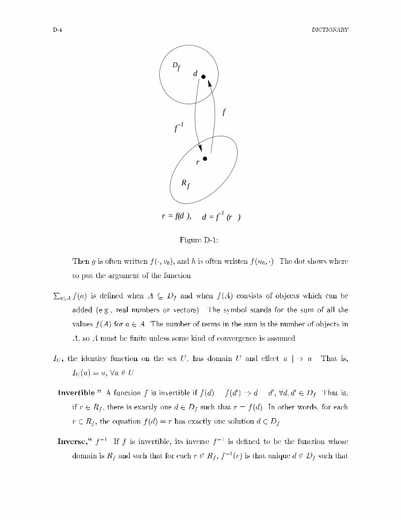
Figure D���
Then g is often written f��� v��� and h is often written f�u�� ��� The dot shows whereto put the argument of the function�
Pa�A f�a� is de�ned when A � Df and when f�A� consists of objects which can be
added �e�g�� real numbers or vectors�� The symbol stands for the sum of all the
values f�A� for a � A� The number of terms in the sum is the number of objects in
A� so A must be �nite unless some kind of convergence is assumed�
IU � the identity function on the set U � has domain U and e�ect u j u� That is�
IU�u� � u� �u � U �
�Invertible�� A function f is invertible if f�d� � f�d��� d � d�� �d� d� � Df � That is�
if r � Rf � there is exactly one d � Df such that r � f�d�� In other words� for each
r � Rf � the equation f�d� � r has exactly one solution d � Df �
�Inverse�� f��� If f is invertible� its inverse f�� is de�ned to be the function whose
domain is Rf and such that for each r � Rf � f���r� is that unique d � Df such that

DICTIONARY D��
f�d� � r� That is� d � f���r� is the unique solution of r � f�d�� Note Df�� � Rf �
Rf�� � Df � See Fig� D���
For example� if the domain is R�� both the functions x j x� and x j x� are
invertible� and their inverses are x j x��� and xj x���� However� if the domain
is R� the function x j x� is not invertible�
Note that if f is invertible� so is f��� and �f����� � f �
Mappings
A Mapping is an ordered triple �U� V� f� in which U and V are sets� f is a function�
Df � U � and Rf � V � We say that �the function f maps U into V �� The mapping
is often abbreviated simply as f if the context makes clear what U and V are�
f � U V is the usual way of writing the mapping �U� V� f� if one wants to note explicitly
what U and V are� The symbol �f � U V � is read �the mapping f of U into V ��
It can also stand for the sentence �f is a function which maps U into V �� In this
latter usage it is equivalent to �f�U� � V ��
F �U V � �� the set of all functions mapping U into V �
Injective� If f is invertible� f � U V is an �injective� mapping or an �injection��
Surjective� If Rf � V � f � U V is a �surjective� mapping or a �surjection��
Bijection� If f � U V is both injective and surjective� it is �bijective�� or a �bijection��
Note� If f � U V is a bijection� so is f�� � V U �
Composition g � f � Suppose f � U V and g � V W � Then g � f � U W is
the mapping de�ned by requiring for each u � U that �g � f��u� � g�f�u��� The
function g � f is called the �composition� of g with f � Note that the order in which
the functions are applied or evaluated runs backward� from right to left�

D�� DICTIONARY
Note� If f � U V and g � V W and h � W X then
h � �g � f� � �h � g� � f� �D���
Note� If f � U V and g � V W are bijections� so is g � f � U W � and
�g � f��� � f�� � g���
Note� If f � U V is a bijection� f�� � f � IU and f � f�� � IV �
Note� Suppose f � U V and g � V U � Then
i� if g � f � IU � then f is an injection�
ii� if f � g � IV � then f is an surjection�
iii� if g � f � IU � and f � g � IV then f is a bijection and g � f���
Note� If f � U V then f � IU � IV � f � f �
Permutations
A permutation is a bijection � � �� � � � � n f�� � � � � ng� It is an �n�permutation� or a
�permutation of degree n��
Sn �� the set of all n�permutations� It has n� members� The product �� of two per�
mutations � and � is de�ned to be their composition� � � �� If e � If������ng then
e� � �e � � and ���� � ���� � e for all � � Sn� These facts� and the above notes
on pg� iv� make Sn a group under the multiplication de�ned by �� � � � �� It is
called the symmetric group of degree n� Its identity is e�
�i� j� transposition or interchange� If i �� j and � � i� j � n �i�e� fi� jg � f�� � � � � ng� then�i� j� stands for the permutation � � Sn such that ��i� � j� ��j� � i� and ��k� � k
if k �� fi� jg� This permutation is called the �transposition� or �interchange� of i
and j� Note that �ij� � �ij� � e� the identity permutation�
Theorem � �See� e�g�� Birkho� and MacLane� A Survey of Modern Algebra�� If
� � Sn� � is the product of n� � or fewer transpositions� There are many ways to

DICTIONARY D�
write � as a product of transpositions� but all have the same parity �i�e�� all involve
an even number of transpositions or all involve an odd number of transpositions��
even� odd� If � � Sn� � is even or odd according as it can be written as the product of
an even or an odd number of transpositions�
sgn � �� �� if � is even� �� �� if � is odd�
Note� sgn ��� � ��� � �sgn ����sgn ���� and sgn e � �� sgn � is read �signum of ���
Note� sgn � � sgn ��� because � � ��� � e� and � � sgn e � sgn � � ��� �
�sgn ���sgn ����� But sgn � � ���
Arrays
An array of order q is a function f whose domain is
Df � f�� � � � � n�g � � � �� f�� � � � � nqg�
The array is said to have dimension n� � n� � � � �� nq�
fi����iq If i� � f�� � � � � n�g� i� � f�� � � � � n�g� � � � � iq � f�� � � � � xqg� then f�i�� � � � � iq� is
often written fi��i�����iq or f i����iq or fi�i�i�
i����iq etc� There are q ways to write it�
The object f�i�� � � � � iq� is called the entry in the array at location �i�� � � � � iq� or
address �i�� � � � � iq�� The integers i�� � � � � iq are the �indices�� and each can be either
a subscript or a superscript� What counts is their right�left order� We will never
use symbols like f ijkl �
�n� is the n�dimensional Kronecker delta� It is an n � n array with �n�ij � � if i �� j�
�n�ij � � if i � j� Usually the n� is omitted� and it is written simply �ij� or �
ij� or
�ij� or �i j�
�n� is the n�dimensional alternating symbol� It is an
n factorsz �� �n� n� � � �� n array� with nn
entries� all � or �� or ��� It is de�ned as follows�

D�� DICTIONARY
�n�i����in � � if any of i�� � � � � in are equal� i�e�� if fi�� � � � � ing �� f�� � � � � ng�
If fi�� � � � � ing � f�� � � � � ng� then there is a unique � � Sn � i� � ����� � � � � in �
��n�� In that case� �n�i����in � �
n��������n� � sgn��
Usually the �n� is written without the n as �i����in � or �i�
i����in � or �i����in � etc�
Example� ��� � �� ��� � �� ��� � ��� ��� � �� �n � �
Example �n � ��
���� � ���� � ���� � �
���� � ���� � ���� � ��
all other �ijk � �� Thus� ���� � �� ���� � �� etc�
Einstein index conventions� i� If an index appears once� without parentheses� in
each term of an equation� the equation is true for all possible values of the
index� Thus� ��ij � �ji� says that ��ij � �ji� for all i� j � f�� � � � � ng� This is
a true statement� ��ijk � �ijk� says that ��ijk � �jik for i� j� k�f�� � � g� Thisis a false statement� The correct statement is �ijk � ��jik�
ii� If an index appears twice in any expression but a sum or di�erence� a sum over
all possible values of that index is understood� Thus� if Aij is an n� n array�
Aii stands forPn
i �Aii� If ui and vj are �rst order arrays of dimension n� uivi
stands forPn
i � uivi� and ui�vi stands forPn
i � ui�vi� but ui � vi and ui � vi
stand for the i�th entries in two arrays� not forP
i�ui � vi� orP
i�ui � vi��
iii� If an index appears three or more times in an expression other than a sum or
di�erence� a mistake has been made� Thus� if Aijkl is an n� n� n� n array�
Aiiii is never written alone� The sum is written out asPn
i �Aiiii�
iv� Parentheses �protect� an index from the conventions� Thus� Aii� refers to a
particular element in the array� the one at location �ii�� And vi� � wi� means
equality only for the particular value of i under discussion� not for all possible
values of i� The element Aiiii in an n � n � n � n array is written Aiiii� to

DICTIONARY D��
make clear that no sum is intended� Strictly speaking� the de�nition of the
Kronecker delta� using these conventions� reads �ij� � � if i �� j� and �ii� � �
for all i�
An array A of order r is symmetric �antisymmetric� in its p�th and q�th indices
if they have the same dimension� np � nq� and
Ai� � � � ip��ipip�� � � � iq��iqiq�� � � � ir
� �Ai� � � � ip��iqip�� � � � iq��ipiq�� � � � ir�
�The � is for symmetric A� the � is for antisymmetric A�� The array is totally
symmetric �antisymmetric� if it is symmetric �antisymmetric� in every pair of
indices�
Some properties of �ij and �i����in are listed below�
�� �ij � �ji
� �n�ii � n
� �ijAjk����kp � Aik����kp for any array A of suitable dimension� �ijAk�jk����kp �
Ak�ik����kp� etc� In particular� �ij�jk � �ik�
�� �i����in is totally antisymmetric�
�� If Ai����in is an
n factorsz �� �n� n� � � �� n array which is totally antisymmetric� there
is a constant � such that
Ai����in � ��i����in�
�� �i����in�j����jn �P
��Sn �sgn�� �i�j���� � � � �i�j��n� �The Polar Identity�� The
two special cases of interest to us are
n � � �ij�kl � �ik�jl � �il�jk which implies �ij�kj � �jk and �ij�ij � �
n � �
�ijk�lmn � �il�jm�kn � �im�jn�kl � �in�jl�km
��im�jl�kn � �il�jn�km � �in�jm�kl

D��� DICTIONARY
which implies �ijk�lmk � �il�jm��im�jl and �ijk�ljk � �il and �ijk�ijk �
��
Some applications of �i����ln are these� If Aij is a real or complex n�n
array whose determinant is detA� then��
Ai�j�Ai�j� � � � Ainjn�j����jn � �detA� �i����in �
In real three�space� suppose x�� x�� x� is a right�handed triple of mutually
perpendicular unit vectors �that is� x� � � x� � x�� � � �� Suppose �u � ui xi
and �v � vj xj� Then
�u � �v � uivi
�u� �v � xi�ijkujvk� or
��u� �v�i �� xi � ��u� �v� � �ijkujvk�
If �r � ri xi is the position vector in real three�space� R�� and �w � R� R�
is a vector �eld� with
�w��r � � wi��r � xi� then
�r � �w � divergence of �w �wi
ri
�r� �w � curl of �w � xi�ijkwk
rj�
A very important general property of arrays is the following�
Remark � Suppose Aijk����kp is antisymmetric in i and j� while Sijl����lq is symmetric in
i and j� Then
Aijk����kP Sijl����lq � ��
Proof�
The subscripts k and l are irrelevant� so we omit them� We have AijSij �
�AjiSji because Aij � �Aji and Sij � Sji� Now replace the summation index

DICTIONARY D���
j by i and the index i by j� Then
AjiSji � AijSij�
Putting these two results together gives AijSij � �AijSij� so AijSij � ��
Vector Space Facts
Fields� A �eld is a set F of objects which can be added� subtracted� multiplied and
divided according to the ordinary rules of arithmetic� Examples are R� C� the set
of rational numbers� and the set of numbers a � bp� where a and b are rational�
We will use only the �elds R and C� and usually F � R�
De�nition of vector spaces� A vector space is an ordered quadruple �V � F � ad� sc�
with these properties�
i� V is a non�empty set� Its members are called vectors�
ii� F is a �eld� Its members are called scalars�
iii� ad � V � V V � This function is called vector addition�
iv� sc � F � V V � This function is called multiplication by scalars�
The remaining properties make more sense if we introduce a new notation� For any
�u��v � V and c � F we de�ne
�u� �v � � ad��u��v�
c�v � �vc �� sc�c� �v�
The additional properties which make �V� F� ad� sc� a vector space are properties of
ad and sc as follows �letters with are vectors� those without are scalars��
v� �u� �v � �v � �u
vi� �u� ��v � �w� � ��u� �v� � �w

D��� DICTIONARY
vii� �a � b��u � a�u� b�u
viii� a��u� �v� � a�u� a�v
ix� a�b�u� � �ab��u
x� ��u � ��v for any �u��v � V
xi� ��u � �u
The vector ��u is called the zero vector� written ��� The vectors �����v and �u������vare written ��v and �u� �v respectively�
Example �� F is a �eld� V is the set of all ordered n�tuples of members of F � so a
typical vector is
�u � �u�� � � � un� with u�� � � � � un � F�
The addition and multiplication functions are
�u� �v �� ad��u��v� �� �u� � v�� � � � � un � vn�
c�v �� sc�c� �v� �� �cv�� � � � � cvn�
The zero vector is �� � ��� � � � � ��� The space V is usually written F n�
Example �� F � R� V is the set of all ordered n tuples of members of R�� so a typical
vector is
�u � �u�� � � � � un� with u�� � � � � un � R��
The addition and multiplication functions are
�u� �v �� ad��u��v� �� �u�v�� � � � � unvn�
c�v �� sc�c� �v� �� �vc�� � � � � vcn��
The zero vector is �� � ��� �� � � � � ���
Example �� Let �V� F� ad� sc� be any vector space and let S be any non�empty set�
De�ne a new vector space �VS� F� adS� scS� as follows�
VS � F�S V�� the set of all functionsf � S V�
DICTIONARY D���
To de�ne adS and scS we note that if f and g are functions in VS and c � F then
adS�f� g� and scS�c� f� are supposed to be functions in VS� i�e�� adS�f� g� � S V
and scS�c� f� � S V � To de�ne these functions� we must say what values they
assign to each s � S� The de�nitions we adopt are these�
�adS�f� g�� �s� � f�s� � g�s� �D��
�scS�c� f�� �s� � cf�s�� �D��
Following the convention for vector spaces� we write adS�f� g� as f �g and scS�c� f�
as cf � Thus� f � g and cf are functions whose domains are S and whose ranges are
subsets of V � The de�nitions ��� and �� read thus� for any s � S
�f � g��s� � f�s� � g�s� �D���
�cf��s� � cf�s�� �D���
These are not �obvious facts�� They are de�nitions of the vector�valued functions
f � g and cf �
In VS� the zero vector is the function which assigns to each s � S the zero vector in
V �
Example �� F � real numbers � R� V � set of all continuous real�valued functions
on the closed unit interval � � x � �� ad and sc are de�ned as in Example �
page D��� �This is a vector space� because if f and g are continuous functions so
is f � g and so is cf for any real c��
Example �� F � R� V � set of all continuous positive real valued functions on
� � x � �� ad and sc as de�ned in Examples and �� This is not a vector space�
There are scalars c � F and vectors f � V such that cf � �V � For example� if f � V
then ����f � �V � In other words� the function sc in this case is not a mapping from
F � V to V �
Notation� Usually the vector space �V� F� ad� sc� will be called simply the vector space
V � We will almost never use the notations ad��u��v� or sc�c� �v�� but will use �u � �v
D��� DICTIONARY
and c�v and �vc� V will be called a vector space over F � or a real or complex vector
space if F � R or C�
Because of vector space rules v� and vi�� there is no ambiguity aboutPn
i � �ui when
�u�� � � � � �un � V � For example� if n � �� all of �u���u����u��u���� ��u���u�����u���u���
��u� � �u�� � �u�� � �u�� ��u� � ��u� � �u��� � �u�� etc�� are the same�
When �u�� � � � � �un � V and a�� � � � � an � F � we do not even need theP� We can use
the index conventions to writePn
i � ai�ui as ai�ui�
Facts about ��� If a � F � then a�� � �� because a�� � a����� � �a���� � ��� � ��� Also� if
a � F � �v � V � and a �� � � �v �� ��� then a�v �� ��� For suppose a�v � �� and a �� ��
Then a�� � F � and �v � ��v � �a��a��v � a���a�v� � a���� � ��� Finally� �� � �u � �u
because �� � �u � ��u� ��u � �� � ���u � ��u � �u�
Linear mappings� Suppose V and W are both vector spaces over the same �eld F � and
L � F�V W �� We call L a �linear mapping� if for any �u� �v � V and c � F it is
true that
L��u� �v� � L��u� � L��v�
L�c�u� � cL��u��
L�V W � is the set of all linear mappings from V to W � �
It is a vector space over F if it�s ad and sc are de�ned as in example � page D���
If L � L�V W � is a bijection� then L�� � L�W V �� And then L is called an
�isomorphism� and V and W are said to be isomorphic� Intuitively speaking� two
isomorphic vector spaces are really the same space� Each member of V corresponds
to exactly one member of W � and vice versa� and ad and sc can be applied in either
V or W with the same result� For example� if F � R� then the two spaces in
examples � and on page D�� are isomorphic� If V is the space in Example �
�Note that if L � L�V �W � and M � L�U � V �� then L �M � L�U � W ��

DICTIONARY D���
then the isomorphism L � Rn V is given by
L�u�� � � � � un� � �eu� � � � � � eun�
and
L���v�� � � � � vn� � �ln v�� � � � ln vn��
Subspaces� A subspace of vector space �V� F� ad� sc� is a vector space � V � F� ad� sc� with
these properties�
i� V � V
ii� fad � ad j eV � eViii� fsc � sc jF � eV �
If V is any subset of V � then � V � F� ad��� eV � eV � sc ���F� eV � is a subspace of �V� F� ad� sc�
if and only if
a� ad� eV � eV � � eV and also
b� sc�F � �V � � eV �
Intuitively� subspaces are lines� planes and hyperplanes in V passing through the
origin� �If eV is a subspace of V � and �v � eV � then ��v � eV by iii�� but ��v � ��� Thus
the zero vector in V is the zero vector in every subspace of V ��
Finite dimensional vector spaces� V is a vector space over �eld F � U is an arbitrary
non�empty subset of V �
Linear combination� If �u�� � � � � �un � V and a�� � � � � an � F � the vector ai�ui is
called a linear combination of f�u�� � � � �ung�
Span� The set of all linear combinations of �nite subsets of U is written sp U � It is
called the span of U � It is a subspace of V � so it is called the subspace spanned
or generated by U � If U is a subspace� U � sp U �
D��� DICTIONARY
Finite dimensional� A vector space V is ��nite dimensional� if V � sp U for
some �nite subset U V �
Linear dependence� A set U � V is �linearly dependent� if there are �nitely
many vectors �u�� � � � � �un � U and scalars a�� � � � � an such that
i� at least one of a�� � � � � an is not �� and also
ii� ai�ui � ���
It is an important theorem that if ��u�� � � � � �un� is a sequence such that f�u�� � � � � �ungis linearly dependent� then there is anm � f�� � � � � ng such that �um � spf�u�� � � � � �um��g�
Linear independence� A set U � V is linearly independent if it is not linearly
dependent� Linear independence of U means that whenever f�u�� � � � �ung � U
and ai�ui � ��� then a� � � � � � an � ��
Basis� Any linearly independent subset of vector space V which spans V is called
a basis for V � The following are important theorems about bases�
Theorem � If V is �nite dimensional� it has a basis� and all its bases are �nite
and contain the same number of vectors� This number is called the dimension
of V � written dimV �
Theorem � If V is �nite dimensional and W is a subspace of V � W is �nite
dimensional and dimW � dimV � Every basis for W is a subset of a basis for
V �
Theorem � If f�u�� � � � � �ung spans V then dimV � n� If dimV � n� then
f�u�� � � � � �ung is linearly independent� hence a basis for V �
Theorem � If V is �nite dimensional and U is a linearly independent subset
of V � U is �nite� say U � f�u�� � � � � �ung� and n � dimV � If n � dimV � U spans
V and so is a basis for V �
Theorem � Suppose B � f�b�� � � ��bng is a basis for V � Then there are func�
tions c�B� � � � � cnB � L�V F � such that for any �v � V
�v � cjB��v��bj�

DICTIONARY D��
The scalars v� � c�B��v�� � � � � vn � cnB��v�� which are uniquely determined by
�v and B� are called the coordinates of �v relative to the basis B� The linear
functions c�B� � � � � cnB are called the coordinate functionals for the basis B� �A
function whose values are scalars is called a �functional��� Clearly �bi � �ij�bj�
Since the coordinates of any vector relative to B are unique� it follows that
cjB��bi� � �i
j �D���
Theorem Suppose V andW are vector spaces over F � and B � f�b�� � � � ��bngis a basis for V � and f�w�� � � � � �wng�W � Then ��L � L�V W � � L��bi� � �wi�
�In other words� L is completely determined by LjB for one basis B� and
LjB can be chosen arbitrarily�� �The L whose existence and uniqueness are
asserted by the theorem is easy to �nd� For any �v � V � L��v� � ciB��v��wi��
This L is an injection if f�w�� � � � � �wng is linearly independent and a surjection
if W � spf�w�� � � � � �wng�
Linear operators� If L � L�V V �� L is called a �linear operator on V �� If B �
f�b�� � � � ��bng is any basis for V � then the array Lij � cjB�L�
�bi�� is called the matrix
of L relative to B� Clearly� L��bi� � Lij�bj� �The matrix of L relative to B is
often de�ned as the transpose of our Lij� It is that matrix � L��bi� � �bjL
ji� Our
de�nition is the more convenient one for continuum mechanics��
The determinant of the matrix of L relative to B depends only on L� not on B� so
it is called the determinant of L� written detL� A linear operator L is invertible
i� detL �� �� If it is invertible it is an isomorphism �a surjection as well as an
injection��
If L � L�V� V �� �v � V � � F � and �v �� ��� and if
L��v� � �v �D���
then is an �eigenvalue� of L� and �v is an �eigenvector�of L belonging to eigenvalue
� The eigenvalues of L are the solution � F of the polynomial equation
det�L� IV � � �� �D���

D��� DICTIONARY
Linear operators on a �nite dimensional complex vector space always have at least
one eigenvalue and eigenvector� On a real vector space this need not be so�
If L and M � L�V� V �� then L �M � L�V� V � and det�L �M� � �detL��detM��
Euclidean Vector Spaces
De�nition� A Euclidean vector space is an ordered quintuple �V�R� ad� sc� dp� with these
properties�
i� �V�R� ad� sc� is a �nite�dimensional �real� vector space
ii� dp is a functional on V � V which is symmetric� positive�de�nite and bilinear�
In more detail� the requirements on dp are these�
a� dp � V � V R� �dp is a functional�
b� dp��u��v� � dp��v� �u� �dp is symmetric�
c� dp��u� �u� � � if �u �� ��� �dp is positive de�nite�
d� for any �u� �v � V � dp��� �v � and dp��u� �� � L�V R�� �dp is bilinear��
dp is called the dot�product functional� and dp��u��v� is usually written �u � �v� In this
notation� the requirements on the dot product are
a�� �u � �v � R �dp is a functional�
b�� �u � �v � �v � �u �dp is symmetric�
c�� �u � �u � � if �u �� �� �dp is positive de�nite�
d�� for any �u� �u�� � � � � �un� �v � V and a�� � � � � an � F
�ai�ui� � �v � ai��ui � �v��v � �ai�ui� � ai��v � �ui�
��� dp is bilinear
Example �� �V�R� ad� sc� is as in Example �� page D��� and �u � �v � uivi� For n �
this is ordinary three�space�

DICTIONARY D���
Example �� �V�R� ad� sc� is as in Example �� page D��� If f and g are two functions in
V � their dot product is f � g �R �� dxf�x�g�x�� Note that without continuity� f �� �
need not imply f � f � �� For example� let f�x� � � in � � x � � except at x � ���
There let f���� � �� Then f �� � but f � f � ��
Length and angle� Schwarz and triangle inequalities� The length of a vector �v in
a Euclidean space is de�ned as k�v k ��p�v � �v� All nonzero�vectors have positive
length� From the de�nitions on page D����
j�u � �vj � k�uk k�vk �Schwarz inequality�
j�u� �vj � k�uk� k�uk �triangle inequality�
If �u �� �� and �v �� �� then �u � �v�k�u kk�v k is a real number between �� and �� so it
is the cosine of exactly one angle between � and �� This angle is called the angle
between �u and �v� and is written � ��u��v�� Thus� by the de�nition of � ��u��v��
�u � �v � k�ukk�vk cos � ��u��v��
In particular� �u � �v � �� � ��u��v� � ��� If k�uk � �� we will write u for �u�
Orthogonality� If V is a Euclidean vector space� and �u��v � V � P � V � Q � V � then
�u��v means �u � �v � ��
�u�Q means �u � �q � � for all �q � Q�
P�Q means �p � �q � � for all �p � P and �q � Q�
Q� �� f�x � �x � V and �x�Qg� This set is called �the orthogonal complement of Q��
It is a subspace of V � Obviously Q�Q�� Slightly less obvious� but true in �nite
dimensional spaces� is �Q��� � spQ�
Theorem Q spans V � Q� �n��o� In particular� if
n�b�� � � � ��bn
ois a basis for
V and �v ��bi � �� then �v � ��� Also� if �v � �x � � for all �x � V � then �v � ���
Orthonormal sets and bases� An orthonormal set Q in V is any set of mutually per�
pendicular unit vectors� I�e�� �u � Q � k�uk � �� and �u��v � Q� �u �� �v � �u � �v � ��

D��� DICTIONARY
An orthonormal set is linearly independent� so in a �nite dimensional Euclidean
space� any orthonormal set is �nite� and can have no more than dimV mem�
bers� An orthonormal basis in V is any basis which is an orthonormal set� If
B � f x�� � � � � xng is an orthonormal basis for V � the coordinate functionals ciB
are given simply by
ciB��v � � �v � xi� ��v � V� �D���
That is� for any �v� �v � ��v � xi� xi�
Theorem Every Euclidean vector space has an orthonormal basis� If U is a
subspace of Euclidean vector space V � U is itself a Euclidean vector space� and
every orthonormal basis for U is a subset of an orthonormal basis for V �
Linear functionals and dual bases� Let V be a Euclidean vector space� For any �v �V we can de�ne a �v � L�V R� by requiring simply
�v��y� � �v � �y� ��y � V� �D����
Theorem �� Let V be a Euclidean vector space� The mapping �v j �v de�ned
by equation ��� is an isomorphism between V and L�V R�� �Therefore we can
think of the linear functionals on V � the members of L�V R�� simply as vectors
in V ��
Proof�
We must show that the mapping �v j �v is an injection� a surjection�
and linear� Linearity is easy to prove� We want to show ai�vi � ai�vi�
But for any �y � V �
ai�vi��y� � �ai�vi� � �y � ai��vi � �y� � ai ��vi��y ��
� �ai�vi���y ��
�See de�nition of ai�vi in example � page D��� Therefore the two func�
tions ai�vi and ai�vi are equal�

DICTIONARY D���
To prove that �v j �v is injective� suppose �u � �v� We want to prove
�u � �v� For any �y � V � we know �u��y� � �v��y�� so �u � �y � �v � �y� or
��u��v� ��y � �� In particular� setting �y � �u��v we see ��u��v� � ��u��v� � ��
so ��u� �v� � ��� �u � �v�
To prove that �v j �v is surjective� let � L�V R�� We want to �nd
a �v � V � � �v� Let f x�� � � � � xng be an orthonormal basis for V and
de�ne �v � � xi� xi� Then for any �y � V � �v��y� � �v � �y � � xi�� xi � �y� �� xi�yi � �yi xi� � ��y�� Thus� �v � � QED�
Even in a Euclidean space� it is sometimes convenient to work with bases which are
not orthonormal� The advantage of an orthonormal basis x�� � � � � xn is that for any
�v � V � �v � ��v � xi� xi� An equation almost as convenient as this can be obtained for
an arbitrary basis� We need some de�nitions� All vectors are in a Euclidean vector
space V �
De�nition� Two sequences of vectors in V � ��u�� � � � � �um� and ��v�� � � � � �vm�� are dual to
each other if �ui � �vj � �ij�
Remark � If ��u�� � � � � �um� and ��v�� � � � � �vm� are dual to each other� each is linearly
independent�
Proof�
If ai�ui � ��� then �ai�ui� � �vj � �� so ai��ui � �vj� � �� so ai�ij � �� so aj � ��
De�nition� An ordered basis for V is a sequence of vectors ��b�� � � � ��bn� such that f�b�� � � � ��bngis a basis for V �
Remark � If two sequences of vectors are dual to each other and one is an ordered
basis� so is the other� �Proof� If ��v�� � � � � �vm� is a basis� m � dimV � Then� since
��u�� � � � � �um� is linearly independent� it is also a basis�

D��� DICTIONARY
Remark � If ��b�� � � � ��bn� is an ordered basis for V � it has at most one dual sequence
��b�� � � � ��bn��
Proof�
If ��b�� � � � ��bn� and ��v�� � � � � �vn� are both dual sequences to ��b�� � � � ��bn�� then
�bi ��bj � �ij� and �vi � bj � �ij� so ��bi��vi� ��bj � �� Then ��bi��vi� � �aj�bj� � �
for any ai� � � � � an � R� But any �u � V can be written �u � aj�bj� so
��bi � �vi� � �u � � for all �u � V � Hence� �bi � �vi � �� �bi � �vi�
Remark � If ��b�� � � � ��bn� is an ordered basis for V � it has at least one dual sequence
��b�� � � � ��bn��
Proof�
Let B � f�b�� � � ��bng� and let ciB be the coordinate functions for this basis�
They are linear functionals on V � so according to theorem ���� there is
exactly one �bi � V such that �bi � ciB� Then �bi��y� � ciB��y �� ��y � V � so
�bi ��y � ciB��y �� ��y � V � In particular� �bi ��bj � ciB��bj� � �i j �see ����� Thus
��b�� � � � ��bn� is dual to ��b�� � � � ��bn��
From the foregoing� it is clear that each ordered basis B � ��bi� � � � ��bn� for V has
exactly one dual sequence BD � ��b�� � � � ��bn� � and that this dual sequence is also an
ordered basis for V � It is called the dual basis for ��b�� � � � ��bn�� It is characterized
and uniquely determined by
�bi ��bj � �i j� �D����
There is an obvious symmetry� each of B and BD is the dual basis for the other�
If �v � V � and B � ��b�� � � � ��bn� is any ordered basis� we can write
�v � vj�bj� �D���

DICTIONARY D���
where vj � cjB��v� are the coordinates of �v relative to B� Then �bi � �v � vj�bi ��bj �
vj�ij � vi� Thus
vi � �bi � �v� �D���
Since ��b�� � � � ��bn� � BD is also an ordered basis for V � we can write
�v � vj�bj� �D����
Because duality is symmetrical� it follows immediately that
vj � �v ��bj� �D����
An orthonormal basis is its own dual basis� it is self�dual� If �bi � xi then �bi � xi�
and ����� ��� are the same as ��� and ����� We have
vj � vj � xj � �v�
In order to keep indices always up or down� it is sometimes convenient to write an
orthonormal basis � x�� � � � � xn� as � x�� � � � � xn�� with xi � xi� Then
vj � vj � xj � �v � xj � �v�
If ��b�� � � � ��bn� � B is an ordered basis for V � and BD � ��b�� � � � ��bn� is its dual basis�
and �v � V � we can write
�v � vi�bi � vi�bi� �D����
The vi are called the contravariant components of �v relative to B� and the vi are the
covariant components of �v relative to B �and also the contravariant components of �v
relative to BD�� The contravariant components of �v relative to B are the coordinates
of �v relative to B� The covariant components of �v relative to B are the coordinates
of �v relative to BD�
The covariant metric matrix of BD is
gij � �bi ��bj� �D����
D��� DICTIONARY
The contravariant metric matrix of BD is
gij � �bi ��bj� �D����
Clearly gij is the contravariant and gij the covariant metric matrix of BD�
We have vi � �bi � �v � �bi � ��bjvj� � ��bi ��bj�vj so
vi � gijvj� �D����
Similarly� or by the symmetry of duality�
vi � gijvj� �D���
The metric matrices can be used to raise or lower the indices on the components of
�v�
Transposes� Suppose V and W are Euclidean vector spaces and L � L�V W �� Then
there is exactly one LT � F�W V � such that
L��v� � �w � �v � LT ��w�� ���v� �w� � V �W� �D���
This LT is linear� i�e� LT � L�W V �� Furthermore� �LT �T � L� and if
a�� � � � � an � R and L�� � � � � Ln � L�V W �� then
�aiLi�T � ai�L
Ti � �D��
The linear mapping LT is called the �transpose� of L �also sometimes the adjoint
of L� but adjoint has a second� quite di�erent� meaning for matrices� so we avoid
the term��
If L � L�V W � and M � L�U V �� then L �M � L�U W � and it is easy to
verify that
�L �M�T � MT � LT � �D��
If L � L�V W � is bijective� then L�� � L�W V �� It is easy to verify that
LT � W V is also bijective and
�L���T � �LT ���� �D���

DICTIONARY D���
Orthogonal operators or isometries� If V is a vector space� the members of L�V V � are called �linear operators on V �� If V is Euclidean and L � L�V V �� then
L is called �orthogonal� or an �isometry� if kL��u�� L��v�k � k�u� �vk for all �u and
�v in V � If L � L�V V �� then each of the following conditions is necessary and
su!cient for L to be an isometry�
a� kL�vk � k�vk� ��v � V
b� L��u� � L��v� � �u � �v� ��u� �v � V
c� LT � L � IV
d� L � LT � IV
e� LT � L��
f� For every orthonormal basis B � V � L�B� is orthonormal� That is� if B �
f x�� � � � � xng is any orthonormal basis� then fL� x��� � � � � L� x�g is also an or�
thonormal basis�
g� There is at least one orthonormal basis B � L�B� is orthonormal�
h� For every orthonormal basis B � V � the matrix of L relative to B has or�
thonormal rows and columns �i�e�� LijL
ik � �jk� and Li
jLkj � �ik��
i� There is at least one orthonormal basis B � V relative to which the matrix
of L has either orthonormal rows �LijL
kj � �ik� or orthonormal columns
�LijL
ik � �ij��
If L is orthogonal� det L � ��� If detL � ��� L is called �proper�� Otherwise L is
�improper��
"�V � �� set of all orthonormal operators on V �
"��V � �� set of all proper orthonormal operators on V �
If L and M � "�V � or "��V �� the same is true of L �M and L��� Also IV � "�V �
and "��V �� Therefore� "�V � and "��V � are both groups if multiplication is de�ned

D��� DICTIONARY
to mean composition� "�V � is called the orthogonal group on V � while "��V � is
the proper orthogonal group�
If L � "��V �� L is a �rotation�� This implies that there is an orthonormal basis
x�� � � � � x�m� x�m�� and angles "�� � � � �"m between � and � such that
L� x�i��� � x�i�� cos �i � x�i sin �i
L� x�i� � � x�i�� sin �i � x�i cos �i
L� x�n��� � x�n���
������������i � f�� � � � � mg
The vector x�n�� is omitted in the above de�nition if dimV is even� and included
if dimV is odd� If included� it is the �axis� of the rotation�
If L � "�V � is improper� L is the product of a rotation and a �re�ection�� A
re�ection is an L for which there is an orthonormal basis x�� � � � � xn such that
L� x�� � � x�� L� xn� � xk� if k � �
Symmetric operators� A symmetric operator on Euclidean space V is an L � L�V� V � �LT � L� �Antisymmetric means LT � �L�� Each of the following conditions is ne�
cessary and su!cient for a linear operator L to be symmetric�
a� LT � L
b� L��u� � �v � L��v� � �u� ��u� �v � V
c� The matrix of L relative to every orthonormal basis for V is symmetric
d� The matrix of L relative to at least one orthonormal basis for V is symmetric�
e� There is an orthonormal basis for V consisting entirely of eigenvectors of L�
That is� there is an orthonormal ordered basis � x�� � � � � xn� for V � and a se�
quence of real numbers ��� � � � � n� �not necessarily di�erent� such that
L� xi�� � i� xi�� �i � f�� � � � � ng� �D���
Facts� The eigenvalues f�� � � � � ng are uniquely determined by L� but the eigenvectors
are not� For any real let ��L��� denote the set of all �v � V such that L��v� � �v�
DICTIONARY D��
Then ��L��� is a subspace of V � and dim ��L��� � � � is an eigenvalue of L� In
that case� ��L��� is called the eigenspace of L with eigenvalue � The eigenspaces
are uniquely determined by L� If � �� �� ��L���� � ��L�����
Positive�de�nite �semide�nite� symmetric operators� If L � L�V V � is sym�
metric� L is said to be positive de�nite when
L��v� � �v � � for all nonzero �v � V �D���
and positive semide�nite when
L��v� � �v � � for all �v � V� �D���
A symmetric linear operator is positive de�nite �semide�nite� i� all its eigenvalues
are positive �non�negative��
Every symmetric positive �semi� de�nite operator L has a unique positive �semi�
de�nite symmetric square root� i�e�� a symmetric positive �semi� de�nite operator
L��� such that
L��� � L��� � L �D���
Polar Decomposition Theorem� �See Halmos� p� ��� ��� Suppose V is Euclidean
and L � L�V V �� Then there exist orthogonal operators O� and O� and positive
semide�nite symmetric operators S� and S� such that
L � O� � S� � S� � O�� �D���
Both S� and S� are uniquely determined by L �in fact S� � �LTL���� and S� �
�LLT ������ If L�� exists� O� and O� are uniquely determined by L and are equal�
and S� and S� are positive de�nite� If detL � � then O� is proper�
The existence part of the polar decomposition theorem can be restated as follows�
for any L � L�V V � there are orthonormal bases � x�� � � � � xn� and � y�� � � � � yn� in
V and non�negative numbers �� � � � � n such that

D��� DICTIONARY
L� xi�� � i� yi�� i � �� � � � � n� �D���
If L is invertible� all i� � ��
Stated this way� the theorem remains true for any L�V W � if V and W are
Euclidean spaces and dimV � dimW � If dimV � dimW � then ��� holds for
i � �� � � � � m� with m � dimW � while for i � m��� � � � � n �with n � dimV � ��� is
replaced by
L� xi� � ��� �D���

Five Prerequisite Proofs
PP��


The Polar Identity
Let Sn �� group all permutations on f�� � � � � ng�
�i������in �� n dimensional alternating symbol
�� � if fi�� � � � � ing �� f�� � � � � ng�� sgn � if i� � ����� � � � � in � ��n�� � � Sn�
Then the polar identity is
X��Sn
� sgn ���i�j���� � � � �inj��n� � �i����in�j����jn� �PP���
Lemma PP�� Suppose Ai����in is an n � � � � � n dimensional n�th order array which is
totally antisymmetric �i�e� changes sign where any two indices are interchanged�� Then
Ai����in � �A�����n� �i����in � �PP��
Proof�
If any two of fi�� � � � � ing are equal� Ai�����in� � �� If they are all di�erent�
there is a � � Sn such that i� � ����� � � � � in � ��n�� This � is a product
of transpositions �interchanges�� and by carrying out these interchanges in
succession on A�����n one obtains A�������n�� Each interchange produces a sign
change� so the �nal sign is � or � according as � is even or odd� Thus�
A�������n� � � sgn��A����n � ��������n�A����n� Therefore� equation PP�� holds
both when fi�� � � � � ing contains a repeated index and when it does not�
PP�

PP�� PROOFS
Lemma PP�� Suppose W is a vector space and f � Sn W and � � Sn� Then
X��Sn
f��� �X��Sn
f����� �X��Sn
f����� �PP��
Proof�
Both the mapping � j ��� and the mapping � j �� are bijections of Sn to
itself� Therefore� each of the sums in �PP�� contains exactly the same terms�
These terms are vectors in W � so they can be added in any order�
Lemma PP�� De�ne
Ai����inj����jn �X��Sn
� sgn���i�j���� � � � �inj��n� �PP���
Then
Ai����inj����jn � Aj����jni����in �PP���
and for any � � Sn�
Ai����inj�������j��n� � � sgn ��Ai����inj����jn �PP���
Proof�
To prove �PP��� note that by lemma � since sgn ��� � sgn ��
Ai����inj����jn �X��Sn
� sgn���i�j������ � � � �inj��� �n��
The set of n pairs ������B� �
������
CA � � � � �
�B� n
����n�
CA���
is the same as the set ������B� ����
�
CA � � � � �
�B� ��n�
n
CA���
because a pair �B� i
j
CA

PROOFS PP��
is in the �rst set of pairs i� j � ����i� and in the second set of pairs i�
i � ��j�� Therefore
�i�j������ � � � �inj����n� � �i����j� � � � �i��n�jn
and
Ai����inj����jn �X��Sn
� sgn ���i����j� � � � �i��n�jn
�X��Sn
� sgn ���j�i���� � � � �jni��n�
� Aj����jni����in �
This proves equation �PP����
To prove equation �PP���� let � � Sn and let j� � k���� � � � � jn � k�n�� Then
from equation �PP����
Ai����ink�������k��n� �X��Sn
� sgn ���i�k����� � � � �ink���n��
Now � sgn ��� � � and so � sgn �� � � sgn���� sgn�� � � sgn �� �� sgn ��� sgn ��� �
� sgn��� sgn ���� and
Ai����ink�������k��n� � � sgn ��X��Sn
� sgn����i�k����� � � � �ink���n�
� � sgn ��X��Sn
� sgn���i�k���� � � � �ink��n� by Lemma PP�
� � sgn ��Ai����ink����kn�
This proves equation �PP����
Now we can prove the polar identity� Let Ai����inj����jn be as in �PP���� Then
�x i�� � � � � in� By lemma � and equation �PP����
Ai����inj����jn � Ai����in�����n�j����jn�
By equation �PP���� interchanging the i�s and j�s gives
Ai����inj����jn � A�����n j����jn�i����in � �PP���

PP�� PROOFS
Set i� � �� � � � � in � n� and equate these two� The result is
A�����n j����jn������n � A�����n�����n�j����jn
so
A�����n j����jn � A�����n �����n�j����jn� �PP���
Substituting �PP��� in �PP��� gives
Ai����inj����jn � A�����n �����n�i����in�j����jn� �PP���
Then from the de�nition �PP���� with ir � r� js � s
A�����n�����n �X��Sn
� sgn������� � � � �n�n��
There are n� terms in this sum� and a term vanishes unless ���� � �� ��� �
� � � � ��n� � n� that is� unless � is the identity permutation e� But sgn e � ��
so only one of the n� terms in the sum is nonzero� and this term is �� Therefore�
A�����n�����n � �� and equation �PP��� becomes the polar identity �PP����
Spectral Decomposition of a
Symmetric Linear Operator S on a
Euclidean Space V �
De�nition PP�� S � V V is symmetric i� S � ST � that is i� �u � S��v� � S��u� � �v for
all �u� �v � V �
Theorem PP��� Let S be a symmetric linear operator on Euclidean space V � Then V
has an orthonormal basis consisting of eigenvectors of S�
Lemma PP�� Suppose S is symmetric� U is a subspace of V � and S�U� � U � Then
S�U�� � U� and SjU� is symmetric as a linear operator on U��
Proof�
Suppose �w � U�� We want to show S��w� � U�� That is� for any �u � U � we
want to show �u �S��w� � �� But �u �S��w� � S��u� � �w� By hypothesis� S��u� � U
and �w � U�� so S��u� � �w � �� Thus� S��w� � U�� Therefore S�U�� � U��
And if the de�nition �PP��� above is satis�ed for all �u� �v � V � it certainly
holds for all �u� �v � U�� Hence� SjU� is symmetric�
Lemma PP�� Suppose S � V V is a symmetric linear operator on Euclidean space
V � Then S has at least one eigenvalue � such that S��v� � ��v� for some �v �� ���
Proof�
PP��

PP�� PROOFS
Let x�� � � � � xn be an orthonormal basis for V � and let Sij be the matrix of
S relative to this basis� so S� xi� � Sij xj� Then Sij � S� xi� � xj � xi �S� xj� � S� xj� � xi � Sji� so Sij is a symmetric matrix� A real number � is
an eigenvalue of S i� det�S � �I� � �� where I is the identity operator on
V � �If the determinant is �� then S � �I is singular� so there is a nonzero
�v � �S � �I���v� � ��� or S��v�� ��v � ��� or S��v� � ��v�� The matrix of S � �I
relative to the basis � x�� � � � � xn� is Sij���ij� so we want to prove that the n�th
degree polynomial in �� det�Sij���ij�� has at least one real zero� It certainlyhas a complex zero� �� so there is a complex n�tuple �r�� � � � � rn� such that
�Sij � ��ij�rj � �� or Sijrj � �ri�
Let � denote complex conjugation� Then
r�iSijrj � ��rir�i �� �PP����
Taking the complex conjugate of this equation gives �Sij is real�
riSijr�j � ���r�i ri��
Changing the summation indices on the left gives
rjSjir�i � ���r�i ri�� �PP����
But Sij � Sji� so the left hand sides of �PP���� and �PP���� are the same�
Also� r�i ri � rir�i �� �� Hence� �� � �� Thus � is real� and we have proved
lemma �PP����
Now we can prove theorem PP��� Let � be any �real� eigenvalue of S� Let v be
a unit eigenvector with this eigenvalue� Then S�spf vg� � spf�vg so by lemma
PP��� S�f vg�� � f vg� and Sjf vg� is symmetric� We proceed by induction on
dimV � Since dimf vg� dimV � we may assume theorem PP�� true on f vg��Adjoining v to the orthonormal basis for f vg� which consists of eigenvectors
of Sjf vg� gives an orthonormal basis for V consisting of eigenvectors of S�
PROOFS PP��
De�nition PP�� Let S be a linear operator on Euclidean space V � A �spectral decom�
position of S� is a collection of real numbers �� � � � �m and a collection of subspaces
of V � U�� � � � � Um� such that
i� SjUi� � �i� IjUi� for i � �� � � � � m
ii� V � U� � � � �� Um� �This means
a� Ui�Uj if i �� j� That is� if �ui � Ui and �uj � Uj then �ui � �uj � ��
b� every �v � V can be written in exactly one way as �v � �u� � � � � � �um with
�ui � Ui� �
Corollary PP�� If S is a symmetric linear operator on Euclidean space V � S has at
least one spectral decomposition�
Proof�
Order the di�erent eigenvalues of S which theorem PP�� produces as ��
� � � �m� Let Ui be the span of all the orthonormal basis vectors turned up
by that theorem which have eigenvalue �i�
Corollary PP�� S has at most one spectral decomposition�
Proof�
Let ���� � � � ��u and U ��� � � � U
�u be a second spectral decomposition� Let ��
be one of ���� � � � � ��u� and let �v � be a corresponding nonzero eigenvector� Then
S��v �� � ���v �� But �v � � �u� � � � � � �um where �ui � Ui� and S��v� � � ���v � �
���u� � � � �� ���um� Hence S��v�� � S��u�� � � � �� S��um� � ���u� � � � �� �m�um�
Hence�
��� � ����u� � � � �� ��� � �m��um � ��� �PP���
Since �v � �� ��� there is at least one �uj �� ��� Then� dotting this �uj into �PP���
gives ��� � �j���uj� � �uj� � �� so �� � �j � �� or �� � �j� Thus every ��i is

PP��� PROOFS
included in f��� � � � � �mg� By symmetry� every �i is included in f���� � � � � ��ug�Therefore the two sets of eigenvalues are equal� and u � m� Since the ei�
genvalues are ordered by size� ��i � �i for i � �� � � � � m� Now suppose
�u � � U �i � Then �u �i � �u� � � � �� �um and S��u �i � � �i��u
�i� � �i��u� � � � �� �um� �
S��u���� � ��S��um� � ����u��� � ���m�um so��i�����u��� � ����i��m��um � ���
Dot in �uj and we get ��i� �j��uj� � �uj� � �� Since �i �� �j� �uj� � �uj� � �� and
�uj � ��� Thus �u�i � �ui� Thus� �u�i � Ui� Thus U
�i � Ui� By symmetry� Ui � U �
i �
Thus Ui � U �i � QED�
Corollary PP�� If a linear operator on a Euclidean space has a spectral decomposition�
it is symmetric�
Proof�
Suppose S has spectral decomposition ���� U��� � � � � ��m� Um�� Let �u��v � V �
We can write �u �Pm
i � �ui� �v �Pm
i � �vi with �ui� �vi � Ui� Then
S��u� �mXi �
S��ui� �mXi �
�i�ui
S��v� �mXi �
S��vi� �mXi �
�i�vi
�u � S��v� �
�mXi �
�ui
���� mXj �
�j�vj
A �mX
i�j �
�j��ui � �vj�
�mXi �
�i��ui � �vi�
S��u� � �v �
�mXi �
�i�ui
���� mXj �
�vj
A �mX
i�j �
�i��ui � �vj�
�mXi �
�i��ui � �vi��
Hence �u � S��v� � S��u� � �v�
Corollary PP�� Two linear operators with the same spectral decomposition are equal�
Proof�

PROOFS PP���
Suppose S and S � have the same spectral decomposition ���� U��� � � � � ��m� Um��
Let �v � V � Then �v �Pm
i � �ui with �ui � Ui� Then
S��v� �mXi �
S��ui� �mXi �
�i�ui �mXi �
S ���ui�
� S ��
mXi �
�ui
�� S ���v��
Since this is true for all �v � V � S � S ��

PP��� PROOFS
Positive De�nite Operators and Their
Square Roots
De�nition PP�� A symmetric linear operator S is positive de�nite if �v � S��v� � � for
all �v �� ��� �S is positive semi�de�nite if �v � S��v� � � for all �v � V ��
Corollary PP�� A symmetric linear operator S is positive �semi� de�nite i� all its
eigenvalues are �non�negative� positive�
Proof�
�� Suppose S has an eigenvalue � � �� Let �v be a nonzero vector with
S��v� � ��v� Then �v � S��v� � ���v � �v� � �� so S is not positive de�nite�
�� Let ���� U��� � � � � ��m� Um� be the spectral decomposition of S� Let ��v � V �
�v �� ��� Then �v �Pm
i � �ui with �ui � Ui and at least one �ui �� ��� Then
S��v� �Pm
i � S��ui� �Pm
i � �i�ui� so
�v � S��v� �
�mXi �
�ui
���� mXj �
�juj
A �mX
i�j �
�j�ui � �uj
�mXi �
�i ��ui � �ui� � ��
Note� The proofs require an obvious modi�cation if S is positive semi�de�nite rather than
positive de�nite�
Theorem PP��� Suppose S is a symmetric� positive �semi� de�nite linear operator in
Euclidean space V � Then there is exactly one symmetric positive �semi� de�nite linear
PP��

PP��� PROOFS
operator Q � V V such that Q� � S� �Q is called the positive square root of S� and is
written S�����
Proof�
Existence� Let ���� U��� � � � � ��m� Um� be the spectral decomposition of S�
Since �i � �� let ����i be the positive square root of �i� Let Q be the linear op�
erator on V whose spectral decomposition is ������ � U��� � � � � ��
���m � Um�� Then
Q is symmetric by corollary PP��� and positive de�nite by corollary PP���
Let �v � V � Then �v �Pm
i � �ui with �u � Ui� Then
Q��v� �mXi �
Q��ui� �mXi �
����i �ui
Q���v� �mXi �
����i Q��ui� �
mXi �
����i �
���i �ui
�mXi �
�i�ui �mXi �
S��ui� � S��v��
Hence� Q� � S�
Uniqueness� Suppose Q is symmetric� positive de�nite� and Q� � S� Let
�q�� U��� � � � � �qu� Uu� be the spectral decomposition of Q� Then if �ui � Ui
we have S��ui� � Q��ui � QQ��ui� � Q�qi��ui�� � q�i��ui�� Thus q�i is an
eigenvalue of S� Therefore �q��� U��� � � � � �q�u� Uu� is a spectral decomposition
for S� Therefore u � m� U � Ui� q�i � �i� Since qi � �� qi � �
���i � Therefore Q
has the spectral decomposition ������ � U��� � � � � ��
���m � Um�� and is the operator
found in the existence part of the proof�

The Polar Decomposition Theorem
Theorem PP��� Suppose V is a Euclidean vector space� L � V V is a linear operator�
and detL � �� Then there are unique linear mappingsR�� S�� R�� S� with these properties�
i� L � R�S�
ii� L � S�R�
iii� R� and R� are proper orthogonal �i�e� R�� � RT and detR � ���
iv� S� and S� are positive de�nite and symmetric�
Further� R� � R�� so S� � RT� S�R��
Before giving the proof we need some lemmas�
Lemma PP�� If det �� �� LTL and LLT are symmetric and positive de�nite�
Proof�
It su!ces to consider LTL� because LLT � �LT �T �LT � and detLT � detL�
First� �LTL�T � LT �LT �T � LTL� so LTL is symmetric� Second� if �v �� ���
L��v� �� �� because L�� exists� But then L��v� � L��v� � �� And L��v� � L��v� ��v � LT �L��v�� � �v � ��LTL���v��� Thus� �v � ��LTL���v�� � �� so LTL is positive
de�nite�
Lemma PP� If S is positive de�nite and symmetric� detS � ��
Proof�
PP���

PP��� PROOFS
Let x�� � � � xn be an orthonormal basis for V consisting of eigenvectors for
S� namely s�� � � � � sn� �Some of these may be the same�� Relative to basis
x�� � � � � xn� the matrix of S is diagonal� and its diagonal entries are s�� � � � � sn�
Therefore detS � s�s� � � � sn� But since S is positive de�nite� all its eigenval�
ues are positive� Therefore detS � ��
Lemma PP� If A and B are linear operators on V and AB � I then B�� exists and
B�� � A� Hence� BA � I and A�� exists and A�� � B�
Proof�
If AB � I then �detA��detB� � detAB � det I � �� so detB �� �� Hence�
B�� exists� By its de�nition� B��B � BB�� � I� And if we multiply
AB � I on the right by B�� we have �AB�B�� � IB��� or A�BB��� � B���
or AI � B��� or A � B��� QED�
Lemma PP� If L is a linear operator on Euclidean space and L�� exists so does �LT ����
and �LT ��� � �L���T �
Proof�
Take transposes in the equation LL�� � I� The result is �L���TLT � I� By
lemma PP��� �LT ��� exists and equals �L���T �
Proof of Theorem PP���
First we deal with R� and S�� To prove these unique� we assume they exist and have
the asserted properties� Then L � R�S� implies LT � �R�S��T � ST
� RT� � S�R
��� so
LTL � S�R��� R�S� � S�IS� � S�
� � Now LTL is a symmetric positive de�nite operator�
and so is S�� Therefore� S� must be the unique symmetric positive de�nite square root of
LTL� i�e�
S� � �LTL����� �PP���

PROOFS PP��
Since detS� � �� S��� exists� Then L � R�S� implies
R� � LS��� � �PP����
Thus S� and R� are given explicitly and uniquely in terms of L� To prove the existence
of an R� and S� with the required properties� we de�ne them by �PP��� and �PP����
Then S� is symmetric positive de�nite as required� and we need show only that R� is
proper orthogonal� i�e� that detR� � �� and RT� � R��
� � But detR� � detL det�S��� � �
detL� detS� � � since detL � � and detS� � �� Therefore� if we can show RT� � R��
� � we
automatically have detR� � �� By lemma PP�� it su!ces to prove RT�R� � I� But RT
� �
�LS��� �T � �S��� �TLT � �ST� �
��LT � S��� LT so RT�R� � S��� LTLS��� � S��� S�
�S��� � I�
Next we deal with R� and S�� To prove them unique� we suppose they exist� Then
L � S�R� so LT � �S�R��
T � RT� S
T� � R��
� S�� But if detL � � then detLT � detL � ��
so there is only one way to write LT � R� S� with R� proper orthogonal and S� symmetric�
If R� is proper orthogonal� so is R��� � and we must have R��
� � R� so R� � R��� �
Then R� and S� are uniquely determined by L� In fact� S� � S� � �LT �TLT � LLT �
and R� � � R���� � �LTS��� ��� � S��L
T ���� To prove existence of R� and S� with
the required properties� we observe that LT � R� S� with R� proper orthogonal and S�
symmetric� Then �LT �T � L � � R� S��
T � S�T RT
� � S�R��� � Therefore we can take
S� � S�� R� � R��� �
Finally� to prove R� � R�� note that if L � S�R� then L � R�R��� S�R� � R��R
T� S�R���
We claim that RT� S�R� is symmetric and positive de�nite� If we can prove that� then
L � R��RT� S�R�� is of the form L � R�S�� and uniqueness of R� and S� requires R� � R��
S� � RT� S�R�� Symmetry is easy� We have �RT
� S�R��T � RT
� ST� �R
T� �
T � RT� S�R�� For
positive de�niteness let �v � V � �v �� ��� Then R���v� �� � because R��� exists� Then
R���v� � S��R���v�� � � because S� is positive de�nite� Then �v � RT� S��R���v�� � �� or
�v � ��RT� S�R����v�� � �� Thus RT
� S�R� is positive de�nite�
We shall not need the PDT when detL � or L�� fails to exist� For these cases� see
Halmos� p� ����

PP��� PROOFS

Representation Theorem for
Orthogonal Operators
De�nition PP�� A linear operator R on Euclidean vector space V is �orthogonal� i� it
preserves length� that is� kR��v�k � k�vk for every �v � V �
There are several other properties each of which completely characterizes orthogonal
operators �i�e�� R is orthogonal i� it is linear and has one of these properties�� We list
them in lemmas�
Lemma PP��� R is orthogonal i� R is linear and preserves all inner products� that is�
R��u� �R��v� � �u � �v for all �u��v � V �
Proof�
Obviously if R preserves all inner products it preserves lengths� The inter�
esting half is that if R preserves lengths then it preserves all inner products�
To see this� we note that for any �u and �v � V � k�u� �vk� � ��u� �v� � ��u� �v� �
�u � �u� �u � �v � �v � �u� �v � �v� That is
k�u� �vk� � k�uk� � �u � �v � k�vk�� �PP����
Applying this result to R��u� and R��v�� and using R��u � �v� � R��u� � R��v��
gives
kR��u� �v�k� � kR��u�k� � R��u� �R��v� � kR��v�k�� �PP����
PP���

PP��� PROOFS
If R preserves all lengths� then kR��u��v�k � k�u��vk� kR��u�k � k�uk� kR��v�k �k�vk� so subtracting �PP���� from �PP���� gives R��u� �R��v� � �u � �v�
Lemma PP��� R is orthogonal i� RT � R��� �Therefore if R is orthogonal R�� exists��
Proof�
If RT � R�� then RTR � I� Then for any �u��v � V � �u � RTR��v� � �u � �v so
R��u� �R��v� � �u ��v� Hence R is orthogonal� Conversely� suppose R orthogonal�
Then for any �u��v � V � R��u� � R��v� � �u � �v� so �u � RTR��v� � �u � �v� so �u ���RTR���v� � �v � � �� Fix �v� Then we see that RTR��v� � �v is orthogonal to
every �u � V � hence to itself� Hence it is ��� so RTR��v� � �v� Since this is true
for every �v � V � RTR � I� Then by lemma PP��� RT � R���
Corollary PP�� If either RTR � I or RRT � I� R is orthogonal�
Proof�
By lemma PP��� either equation implies RT � R���
Corollary PP� If R is orthogonal� so is R���
Proof�
By lemma PP���� R�� exists and is RT � But RT �RT �T � RTR � I� so RT
satis�es the second equation in corollary PP��� Hence RT is orthogonal�
The easiest way to discover whether a linear R � V V is orthogonal is to study its
matrix Rij relative to some orthonormal basis for V � Recall that we de�ne this matrix by
R� x�i � Rij xj �PP����
where � x�� � � � � xn� is the orthonormal basis for V which we are using� The matrix Lij of
an arbitrary linear operator L is de�ned in the same way�
L� x�i � Lij xj� �PP����

PROOFS PP���
The matrix of LT relative to � x�� � � � � xn� is the transposed matrix Lji� That is
LT � xi� � Lij xj or �LT �ij � Lji� �PP����
To see this� we note that xk � L� xi� � Lij xk � xj � Lij�kj � Lik� so
Lij � L� xi� � xj� �PP���
Therefore �LT �ij � LT � xi� � xj � xi � L� xj� � Lji�
Now we have
Remark � If R is orthogonal� then its matrix relative to every orthonormal basis satis�es
RijRik � �jk ��orthonormal columns�� �PP���
and
RjiRki � �jk ��orthonormal rows�� �PP��
Proof�
If R is orthogonal so is RT � Therefore� it su!ces to prove �PP���� We have
RT � xj� � �RT �ji xi � Rij xi� Then RRT � xj� � RijR� xi� � RijRik xk� But if
R is orthogonal� RRT � I� so RRT � xj� � �jk xk� Thus RijRik xk � �jk xk� or
�RijRik � �jk� xk � �� Fix j� Since x�� � � � � xn are linearly independent� we
must have RijRik � �jk � �� This is �PP����
Remark If R � L�V V � and there is one orthonormal basis for V relative to which
the matrix of R satis�es either �PP��� or �PP��� then R is orthogonal�
Proof�
Suppose that relative to the particular basis x�� � � � � xn� the matrix ofR satis�es
�PP���� Multiply by xk and add over k� using Rik xk � R� xi�� The result is
RijR� xi� � xj�

PP��� PROOFS
By linearity ofR� this meansR�Rij xi� � xj orRhRT � xj�
i� xj� or �RR
T �� xj� �
xj� But then for any scalars v�� � � � � �vn we have �RRT ��vj xj� � vjRRT � xj� �
vj xj� Hence RRT ��v� � �v for all �v � V � Hence RRT � I� Hence R is
orthogonal�
Next suppose R satis�es �PP�� rather than �PP���� Then �RT �ij�RT �ik �
�jk� so the matrix of RT satis�es �PP���� Hence� RT � R�� is orthogonal�
Hence so is �RT �T � �R����� � R�
Corollary PP� If the rows of a square matrix are orthonormal� so are the columns�
A matrix with this property is called orthogonal� What we have seen is that if R is
orthogonal� so is its matrix relative to every orthonormal basis� And if the matrix of R
relative to one orthonormal basis is orthogonal� R is orthogonal� so its matrix relative to
every orthonormal basis is orthogonal�
Now we discuss some properties of orthogonal operators which will eventually tell us
what those operators look like�
First� we introduce the notation in
De�nition PP�� The set of all orthogonal operators on Euclidean space V is written
"�V �� The set of all proper orthogonal operators �those with determinant � �� is written
"��V ��
Lemma PP��� "�V � and "��V � are groups if multiplication is de�ned as operator
composition�
Proof�
All we need to prove is that both sets are closed under the operations of taking
inverses and of multiplying� But ifR � "�V �� we know R�� � "�V � by remark
PP�� And det�R��� � �detR��� � � if detR � � so if R � "��V � then
R�� � "��V �� If R� and R� � "�V �� then �R�R��T �R�R�� � RT
�RT�R�R� �
RT� IR� � RT
�R� � I� so R�R� � "�V �� And if R�� R� � "��V � then
det�R�R�� � �detR���detR�� � �� so R�R� � "��V ��

PROOFS PP���
Lemma PP��� If R � "�V �� detR � �� or ���
Proof�
RTR � I so �detRT ��detR� � det I� But detRT � detR and det I � ��
Thus �detR�� � ��
Lemma PP��� Suppose R � "�V � and U is a subspace of V and R�U� � U � Then
RjU � "�U��
Proof�
By hypothesis� RjU is a linear operator on U � Since kR��v�k � k�vk for all
�v � V � this is certainly true for all �v � U � Hence� RjU satis�es de�nition
PP��
Lemma PP��� Under the hypothesis of lemma PP���� RT �U� � U �
Proof�
Suppose �u � U � Then there is a unique �u � � U such that �u � �RjU���u �� �be�
cause �RjU��� exists as a linear operator on U�� But �u � � U � so �RjU���u �� �
R��u ��� Thus �u � R��u ��� and R����u� � �u �� Then RT ��u� � �u �� Thus
RT ��u� � U if �u � U � QED
Lemma PP��� Under the hypotheses of lemma PP���� R�U�� � U��
Proof�
Suppose �w � U�� We want to show R��w� � U�� That is� �u �R��w� � � for all
�u � U � But �u �R��w� � RT ��u� � �w� By lemma PP��� RT ��u� � U � By hypothesis
�w�U � Hence� RT ��u� � �w � �� as required�
Lemma PP�� If R � "�V � and is an eigenvalue of R� � ���
Proof�

PP��� PROOFS
Suppose R��v� � �v and �v �� ��� Then k�vk � kR��v�k � k�vk �j j k�vk so
� �j j� QED�
Lemma PP�� Let R � "�V �� Let x�� � � � xn be an orthonormal basis for V � Let Rij
be the matrix of R relative to this basis� Suppose is a complex zero of the n�th degree
polynomial det�Rij � �ij�� Then j j�� ��
Proof�
There is a complex n�tuple �r�� � � � � rn� �� ��� � � � � �� such that Rijrj � ri�
Taking complex conjugates gives Rijr�j � �r�i � or Rikr
�k � �r�i � Multiplying
and summing over i gives
RijRikrjr�k � �rir
�i �
But RijRik � �jk� so rjr�j �j j� rir�i � Since rir�i � �� we have j j�� ��
Lemma PP�� In lemma PP���� � is also a zero of det�Rij � �ij� � ��
Proof�
Since �Rij � ��ij�r�j � � and �r��� � � � � r
�n� �� ��� � � � ��� det�Rij � ��ij� � ��
Lemma PP��� Suppose R� Rij as in lemma PP���� Suppose is not real and �r�� � � � � rn� ����� � � � � �� is a sequence of n complex numbers such that Rijrj � ri� Then riri � ��
Proof�
Rikrk � ri so �Rijrj��Rikrk� � �riri� or RijRikrjrk � �riri� or �jkrjrk �
�riri� or rjrj � �riri� or ��� ��riri � �� Since is not real� �� � �� �� so
riri � ��
Remark Suppose R � "�V � and V contains no eigenvectors of R� Then V contains
two mutually orthogonal unit vectors �x and �y such that for some � in � � ��

PROOFS PP���
�������������R� x� � x cos" � y sin"
R� y� � x sin" � y cos"�
�PP��
Proof�
Choose an orthonormal basis z�� � � � � zn for V � and let Rij be the matrix of
R relative to that basis� If � � det�Rij � �ij� has a real root� � it is an
eigenvalue of R� so R has an eigenvector� Hence no root of det�Rij � �ij�
is real� By lemma PP���� we can write any root as ei� where � � � or
� � �� By lemma PP���� we can �nd a root e�i� with � � �� Then
there is an n�tuple of complex numbers �r�� � � � � rn� �� ��� � � � � �� such that
Rjkrj � e�i�rk� �PP���
We may normalize �r�� � � � � rn� so that
r�jrj � �PP���
and by lemma PP��
rjrj � �� �PP���
Now write rj � xj � iyj where xj and yj are real�
Then separating the real and imaginary parts of �PP��� gives
Rjkxj � xk cos � � yk sin �
Rjkyj � �xk sin � � yk cos ��
Separating the real and imaginary parts of �PP��� gives
xjxj � yjyj � �
xjyj � �

PP��� PROOFS
and �PP��� gives
xjxj � yjyj � �
From these equations� clearly
xjxj � yjyj � � and xjyj � ��
Now take x � xj zj and y � yj zj� and we have the x� y� � whose existence is asserted in
the theorem�
Corollary PP� dimV � �
Remark Suppose R � "�V � and V contains no eigenvectors of R� Then V has an
orthonormal basis x�� y�� � � � xm� ym such that for each j � f� � � � � mg there is an "j in
� �j � with
�������������R� xj� � xj� cos �j� � yj� sin �j�
R� yj� � � xj� sin �j� � yj� cos �j�
� �PP���
Proof�
By remark PP�� we can �nd mutually orthogonal unit vectors x�� y� and ��
in � �� � such that �PP��� holds for j � �� Then R�spf x�� y�g� �spf x�� y�g� Hence� by lemma PP���� R�f x�� y�g�� � f x�� y�g�� Hence� by
lemma PP���� Rjf x�� y�g� � "�f x�� y�g��� Since R has no eigenvectors in V �
it has none in f x�� y�g�� Thus Rjf x�� y�g� satis�es the hypotheses of remark
PP�� and we can repeat the argument� �nding �� in � �� � an mutually
orthogonal unit vectors x�� y� in f x�� y�g� such that �PP��� holds for j � �
We can proceed in this way as long as the dimension of the remaining space
is � �� �The argument is by induction on dimV �� When the dimension of the
remaining space is �� we have an orthonormal basis for V with the required
properties�

PROOFS PP��
Corollary PP��� dimV is even� That is� if R � "�V � and dimV is odd� R has an
eigenvector� �This is obvious from another point of view� If dimV is odd� so is the degree
of the real polynomial det�R� I�� Hence� it has at least one real zero��
Theorem PP��� Suppose V is Euclidean vector space and R � "�V �� Then V has an
orthonormal basis x�� y�� � � � � xm� ym� z�� � � � zn� w� � � � � wp with these properties�
i� R� wj� � � wj
ii� R� zj� � zj
iii� for j � f�� � � � � mg� there is a �j in � �j � such that equation �PP��� holds�
Proof�
Let Z and W be the eigenspaces of V with eigenvalues �� and ��� Let
z�� � � � � zn be an orthonormal basis for Z and w�� � � � � wp an orthonormal basis
for W � Then R�Z �W � � Z �W � so R��Z �W ��� � �Z �W ��� Moreover�
�Z �W �� contains no eigenvectors of R� since all their eigenvalues are �� or
��� and these are already in Z orW � Thus remark PP�� applied to �Z�W ���
QED�
Corollary PP��� detR � ����p�
Proof�
Relative to the basis in theorem PP���� the matrix of R looks thus�
Each � diagonal block contributes a factor cos� �j � sin� �j � � to the
determinant� whence the result�

PP��� PROOFS
. . .
cosθ sin θ
θ-sin cosθ
1
1
. . .
-1 . . .{
cos sin
-sin cos
cosθ sin θ
θ-sin cosθ
1 1
1 1
θ θ
θ θ
2 2
2 2
m m
m m
n
p
terms
terms {-1
Figure PP��� Matrix of R�
PROOFS PP���
Corollary PP��� IfR � "��V �� then V has an orthonormal basis x�� y�� � � � � xm� ym� z�� � � � � zn
such that�����������������������������������������
i� R� zj� � zj for j � f�� � � � � ng�
ii� For j � f�� � � � � mg there is a �j in � �j � � such that
R� xj� � xj� cos �j� � yj� sin �j�
R� yj� � � xj� sin �j� � yj� cos �j��
� �PP���
Proof�
Since detR � ��� in theorem PP���� p is even� Therefore� we may divide
w�� � � � � wp into pairs� For any such pair� we have �for example�
R� w�� � � w� � w� cos � � w� sin �
R� w�� � � w� � � w� sin � � w� cos ��
If we adjoin these pairs to the pairs � xj� yj� given by theorem PP���� and take the
corresponding angles as � � �� we have the result of the corollary�
For obvious reasons� a linear operator on V which looks like �PP��� in some or�
thonormal basis is called a �rotation�� Corollary PP�� says that every proper orthogonal
operator is a rotation� If dimV � � the eigenvector z� is called the axis of the rotation�
and the angle #�� in � �� � � is the angle of the rotation� This terminology breaks down
only when m � � and n � in �PP���� In that case� R � I� The angle of rotation of I
is �� but its axis of rotation obviously cannot be de�ned�
For dimV � � corollary PP�� is called Euler�s theorem� If R � L�V V � and an
orthonormal basis x�� � � � � xn for V can be found such that R� x�� � � x�� R� xj� � xj for
j � then R is said to be a re�ection along x�� Obviously detR � �� for a re�ection�

PP��� PROOFS
so a re�ection is an �improper orthogonal� operator� Also� clearly a re�ection has the
property R�� � R� or R� � I�
If R� is a re�ection and R� is any other improper orthogonal operator� then R � R�R�
is orthogonal and detR � �det�R���detR�� � ����� � �� so R is proper orthogonal� But
then R�R � R��R� � R�� so R� � R�R� That is� every improper orthogonal operator is
the product of a rotation and a re�ection�
Part I
Tensors over Euclidean Vector Spaces
�


Chapter �
Multilinear Mappings
��� De�nition of multilinear mappings
M�V� � � � �� Vq W ��
V�� � � � � Vq�W are vector spaces over a single �eld F � and M � F �V�� � � ��Vq W ��
If M satis�es any of the following three equivalent conditions� M is called a multilinear
mapping from V� � � � �� Vq to W �
De�nition ����� For any ��v�� � � � � �vq� � V� � � � �� Vq and any p � f�� � � � � qg�
M��v�� � � � � �vp��� �� �vp��� � � � � �vq� � L�Vp W ��
�That is� M��v�� � � � � �vq� depends linearly on each of the separate vectors �v�� � � � � �vq if the
others are held �xed��
De�nition ���� If a � F � p � f�� � � � � qg� �xp and �yp � Vp� and ��v�� � � � � �vq� � V��� � ��Vqthen
i� M��v�� � � � � �vp��� a�vp� �vp��� � � � � �vq� � aM��v�� � � � � �vp��� �vp� �vp�n� � � � � �vq�� Also
ii� M��v�� � � � � �vp��� �xp � �yp� �vp��� � � � � �vq� � M��v�� � � � � �vp��� �xp� �vp��� � � � � �vq�
�M��v�� � � � � �vp��� �yp� �vP��� � � � � �vq� �
� CHAPTER �� MULTILINEAR MAPPINGS
De�nition ���� For each p � f�� � � � � qg� suppose a�p�� � � � � anpp� � F and �vp�� � � � � � �v p�
np �Vp� Then M
�ai����v
��i� � � � � � a
iqq��v
q�iq
�� ai��� � � � a
iqq�M
��v��i� � � � � � �v
q�iq
��
De�nition ���� M�V� � � � � � Vq W � denotes the set of all multilinear mappings
from V� � � � �� Vq to W �
��� Examples of multilinear mappings
In these examples� V�� � � � � Vq are Euclidean vector spaces� and the �eld F is R� The
vector space W need not be Euclidean �i�e� need not have a dot product� but it must be
real �i�e� its �eld is R��
Example ����� For each p between � and q� let �up be a �xed vector in Vp� Let �w� � W �
For any ��v�� � � � � �vq� � V� � � � �� Vq� de�ne
M��v�� � � � � �vq� � ��u� � �v�� � � � ��uq � �vq��w�� ������
To give the next example� some terminology is useful� Suppose that for each p �f�� � � � � qg Bp �
��bp�� � � � � ��b p�np
�is an ordered basis for Vp� Then the sequence of ordered
bases �B�� � � � � Bq� is called a �basis sequence� for V�� � � ��Vq� Let BDp � ��b �p�� � � � �
�bnpp��
be the ordered basis for Vp which is dual to Bp� Then �BD� � � � � � B
Dq � is �the basis sequence
dual to �B�� � � � � Bq���
Example ����� Let �B�� � � � � Bq� be a basis sequence for V�� � � ��Vq� Let �wi����iq be any
q�th order� n� � � � � � nq array of vectors from W � For any ��V�� � � � � �Vq� � V� � � � �� Vq
de�ne
M��v��� � � � � �vq�
����b i��� � �v ��
�� � �
��biqq� � �vq�
��wi����iq � �����
Then
M � M �V� � � � �� Vq W � �����
and also
M��b��j� � � � ��b
��jq
�� �wj����jq � ������

���� EXAMPLES OF MULTILINEAR MAPPINGS �
The multilinearity of M is almost obvious� ����� is a sum of n�n� � � � nq terms like
������� Each of these terms is linear in each �vp if �v�� � � � � �vp��� �vp��� � � � �vq are �xed�
To prove ������ we let �vp � �bp�jp in the de�nition ������ obtaining M��b
��j� � � � � �
�bq�jq � �
��b i�����b ��j� � � � � ��biqq���b q�jq ��wi����iq � �i� j� � � � �
iqjq �wi����iq � �wj����jq � There are no other examples�
Every member ofM�V� � � � �� Vq W � is like example ������ We have
Remark ������ Suppose V�� � � � � Vq are Euclidean vector spaces and W is a real vector
space� Suppose dimV� � n�� � � � � dimVq � nq� Suppose �B�� � � � � Bq� is a basis sequence
for V� � � � �� Vq� and �wi����iq is an n� � n� � � � �� nq array of vectors from W � Then ��M � M�V� � � � �� Vq W � �M��b
��i� � � � � ��b
q�iq � � �wi����iq �
Proof�
Example ��� shows at least one such M � To establish uniqueness suppose
M does satisfy ����� and ������� Let ��b�p�� � � � ��bnpp�� � BD
p be the ordered
basis for Vp which is dual to Bp � ��bp�� � � � � ��b p�np �� For any �vp� � Vp� we have
�vp� � vipp��bp�ip where �v
ipp� � vp� ��bipp� � Then
M��v��� � � � � �v q�� � M�vi����b��i� � � � � � v
iqq��bq�iq � �by de�nition ������
� bi��� � � � viqq�M��b
��i� � � � � ��b
q�iq � �by hypothesis�
� vi��� � � � viqq� �wi����iq
���bi��� � �v��
�� � �
��biqq� � �vq�
��wi����iq �
In other words� M is the function de�ned by ������
It follows that every M � M�V� � � � �� Vq W � has the form ������

� CHAPTER �� MULTILINEAR MAPPINGS
��� Elementary properties of multilinear mappings
Remark ������ If one of �v�� � � � � �vq is �� and if M � M�V� � � � � � Vq W � then
M��v�� � � � � �vq� � ��� the zero in W �
Proof�
We suppose �v� � ��� ThenM���� �v�� � � � � �vq� � M����� �v�� � � � � �vq� � �M���� �v�� � � � � �vq� �
��� where we have used de�nition ��������
Remark ������ M�V� � � � �� Vq W � is a vector space over F if we use the ad and
sc de�ned in example � page D��� or in equations ������� ������
Proof�
Refer to �subspaces� on page D���� We know from example � page D���
that F �V� � � � � � Vq W � is a vector space over F � Obviously� M�V� �� � �� Vq W �� is a subset of F �V� � � � �� V q� W �� Therefore� it su!ces
to prove that if a � F and M � N � M�V� � � � � � V q W �� then aM and
M � N � M�V� � � � � � Vq W �� That is� if M and N are multilinear� so
are aM and M �N � This is immediate from de�nition ����� because we know
it for linear functions� Alternatively� we can use de�nition ����� and write
everything out� We will do this for M �N � We have
�M �N��a i����v
��i� � � � � � a
iqq��v
q�iq
�� M
�ai����v
��i� � � � � a
iqq��v
q�iq
��N
�a i����v
��i� � � � � � a
iqq��v
q�iq
�� by de�nition of M �N�
� a i��� � � � a
iqq�M
��v��i� � � � � � �v
q�iq
�� ai��� � � � a
iqq�N
��v��i� � � � � � �v
q�iq
��because M and N are multilinear�
� a i��� � � � aiqa�
hM��v��i� � � � � � �v
q�iq
��N
��v��i� � � � � � �vq�iq
�ibecause W is a vector space over F

���� PERMUTING A MULTILINEAR MAPPING
� ai��� � � � aiqq�
h�M �N�
��v��i� � � � � � �v
q�iq
�iby de�nition of M �N�
Comparing the two ends of this chain of equalities� we have a proof thatM�N
is multilinear if M and N are� and if M �N is de�ned by �������
�� Permuting a multilinear mapping
De�nition ������ Suppose ��v�� � � � � �vq� � V� � � � � � Vq and � � r s � q� The q�
tuple ��v�� � � � � �vr��� �vs� �vr�� � � � � �vs��� �vr� �vs��� � � ��vq� will be abbreviated ��v�� � � ��vq�rs�� It is
simply ��v�� � � � � �vq� with �vr and �vs interchanged� Note that if Vr � Vs� then ��v�� � � � � �vq�rs� �V� � � � �� Vq�
De�nition ������ Suppose M � M�V� � � � � � Vq W � and � � r s � q� Suppose
Vr � Vs� Then we write �rs�M for the member of F �V� � � � � � Vq W � de�ned by
requiring for any ��v�� � � � � �vq� � V� � � � �� Vq that
��rs�M � ��v�� � � � � �vq� � M ��v�� � � � � �vq�rs� � �������
That is
��rs�M � ��v�� � � � � �vr��� �vr� �vr��� � � � � �vs��� �vs� �ss��� � � � � �vq�
� M ��v�� � � � � �vr��� �vs� �vr��� � � � � �vs��� �vr� �ss��� � � � � �vq� � ������
Remark ������ �rs�M � M�V� � � � �� Vq W � if Vr � Vs�
Proof�
Obvious from ������ and de�nition ��������
Remark ������ �rs� is a linear operator onM�V� � � � �� Vq W � if Vr � Vs�

� CHAPTER �� MULTILINEAR MAPPINGS
Proof�
By remark �������� �rs� � M�V�� � � ��Vq W � M�V�� � � ��Vq W ��
It remains to prove that �rs� is linear� Suppose a�� � � � � aN are scalars and
M�� � � �MN � M�V� � � � �� Vq W �� We want to prove that �rs��ajMj� �
aj��rs�Mj�� Let ��v�� � � � � �vq � V� � � � �� Vq�� Then
��rs��ajMj�� ��v�� � � � � �vq� � �ajMj���v�� � � � � �vq�rs� � ajhMj��v�� � � � � �vq�rs�
i
� aj
�h�rs�Mj
i��v�� � � � � �vq�
���ajh�rs�Mj
i���v�� � � � � �vq��
Since this is true for any ��v�� � � � � �vq� � V� � � � � � Vq� we have the required
result�
De�nition ������ Suppose M � r� s as in de�nition ������� If �rs�M � M � M is �sym�
metric� under �rs�� If �rs�M � �M � M is �antisymmetric� under �rs��
Remark ������ If Vr � Vs� the members ofM�V�� � � ��Vq W � which are symmetric
under �rs� constitute a subspace of M�V� � � � � � Vq W �� The same holds for the
members antisymmetric under �rs��
Proof�
It su!ces to show that if a is any scalar and M � N are symmetric �or antisym�
metric� under �rs�� so are aM andM�N � We give the proof for antisymmetry�
In that case� by hypothesis�
�rs�M � �M � �rs�N � �N�
But �rs� is linear� so �rs��aM � � a��rs�M � � a��M� � �aM � and �rs��M �
N� � �rs�M��rs�N � �M�N � ��M�N�� �Note that the set of members
ofM�V� � � � �� Vq W � which are symmetric �anti�symmetric� under �rs�
is simply the eigenspace of �rs� with eigenvalue ������ Of course� it is a
subspace ofM�V� � � � �� Vq W ���

���� PERMUTING A MULTILINEAR MAPPING �
De�nition ������ Suppose V� � � � � � Vq � V � Suppose M � M��qV W � and
� � Sq� Then �M is de�ned as that member of F��qV W � such that for any
�v�� � � ��vq � V
��M���v�� � � � � �vq� � M��v���� � � � � �v�q�
��
Remark ������ If V� � � � � � Vq � V then �M � M��qV W �� and in fact � is a
linear operator onM��qV W �� Moreover if �� � � Sq and M � M��qV W � then
���M� � ����M� ������
Proof�
Except for ������� the proof is like that of remark ��������� To prove equation
������� let �v�� � � � � �vq � V and let �w� � �v���� � � � � �wq � �v�q�� Then����M�
���v�� � � � � �vq� � ��M�
��v���� � � � � �v�q�
�
� ��M� ��w�� � � � � �wq� � M��w���� � � � � �w�q�
�
� M��v������� � � � � �v���q��
�
� M��v������ � � � � �v���q�
�
� �����M � ��v�� � � � � �vq�
Since this is true for all �v�� � � � � �vq � V � we have �������
De�nition ������ Suppose V� � � � � � Vq � V and M � M � ��qV W �� M is
totally symmetric �antisymmetric� if �M � M ��M � � sgn��M � for every � � Sq�

�� CHAPTER �� MULTILINEAR MAPPINGS
Remark ����� M is totally symmetric �antisymmetric� i� �rs�M � M�� �M� for
every transposition �rs��
Proof�
�� is obvious� For��� recall that any � � Sq is a product of transpositions�
By remark ������ the e�ects of these transpositions on M can be calculated
one after the other� If all leave M unchanged� so does �� If all multiply M by
��� then �M is M multiplied by sgn � �� �� for even�odd ���
Remark ����� The totally symmetric �antisymmetric� members of M��qV W �
constitute a subspace ofM��qV W ��
Proof�
We give the proof for the totally symmetric case� Suppose M�� � � � �MN are
totally antisymmetric members ofM��qV W � and a�� � � � � aM are scalars�
We want to show that aiMi is totally antisymmetric� But for any � � Sq� � is
linear operator on M��qV W �� so ��aiMi� � ai��Mi� � ai�� sgn��Mi� �
� sgn���aiMi�� That is� aiMi is totally antisymmetric�

Chapter �
De�nition of Tensors over Euclidean
Vector Spaces
If V�� � � � � Vq are Euclidean vector spaces� thenM�V�� � � ��Vq� R is called the �tensor
product of V�� � � � � Vq�� It is written V� � � � �� Vq� Thus
V� � � � �� Vq ��M�V� � � � �� Vq� R� ������
The multilinear functionals which are the members of V�� � � �� Vq are called the tensors
of order q over V� � � � �� Vq�
If V� � � � � � Vq � V � then V�� � � �� Vq �
q timesz �� �V � � � �� V � and this is abbreviated �qV �
Its members are called the tensors of order q over V � By convention� tensors of order zero
are scalars� that is
��V � R� �����
For tensors of order �� the notation requires some comment� When q � �� multilinearity
is simply linearity� That is M�V R� � L�V R�� Thus the tensors of order � over
a vector space V are simply the linear functional on V � This would not be a problem�
except that for q � �� ������ reduces to V� ��M�V� R�� which says
V � L�V R�� �����
��
�� CHAPTER �� DEFINITION OF TENSORS OVER EUCLIDEAN VECTOR SPACES
It is at this point that we require V to be a Euclidean vector space� If it is� then �v � V can
be safely confused with the linear functional �v � L�V R� de�ned by ����� Tensors
of order � over V are simply the vectors in V �
When V is not a Euclidean vector space� ����� is false� �The situation is very
subtle� If V is not Euclidean but is �nite dimensional� every basis B for V generates an
isomorphism between V and L�V R�� namely�bij ciB� But each of these isomorphisms
depends on the basis B chosen to produce it� There is no �natural�� basis�independent
isomorphism which can be used to identify vectors with linear functionals� See MacLane
and Birkho�� Algebra� MacMillan ����� p� � for a more detailed discussion�� Tensors
over vector spaces which are not Euclidean are constructed in a more complicated fashion
than ������� We will not need this generality� and tensors over Euclidean spaces have
some very useful properties for continuum mechanics� It is for this reason that we consider
only tensors over Euclidean spaces� See M� Marcus�s book� on reserve� for a treatment of
tensors over arbitrary vector spaces�

Chapter �
Alternating Tensors� Determinants�
Orientation� and n�dimensional
Right�handedness
In this section we discuss an application of tensors which some of you may have seen in
your linear algebra courses�
Let V be an n�dimensional Euclidean vector space� The set of totally antisymmetric
tensors of order q over V is written �qV � It is a subspace of �qV � �See remark ��������
We want to study �nV � The members of �nV are called �alternating tensors over V ��
��� Structure of �nV
We want to understand what the alternating tensors over V are like� It will turn out that
there are not very many of them� In fact dim�nV � �� We want to prove this and to
�nd a basis �vector� in the vector space �nV �
First we note a technique for verifying that A � �nV � We need to prove only that
A � �nV and that �rs�A � �A for every transposition �rs� � Sn� If this latter fact is
true� then clearly remark ���� tells us A � �nV �
A second property of an A � �nV which is equivalent to membership in �nV is that
�

��CHAPTER �� ALTERNATING TENSORS� DETERMINANTS� ORIENTATION� ANDN�DIMENSIONAL RIGHT�HANDEDNESS
for any ��v�� � � � � �vn� � �nV and any � � Sn�
A��v���� � � � � �v�n�
�� � sgn ��A ��v�� � � � �vn� � ������
This is obvious from the de�nition of �A and �nV � It implies the �rst step in our
attempt to understand alternating tensors�
Lemma ������ If A � �nV and two of �v�� � � � �vn are equal� then A��v�� � � � � �vn� � ��
Proof�
If �vr � �vs� interchanging them will not change A��v�� � � � � �vn�� But sgn �rs� �
��� so ������ says interchanging them changes the sign of A��v�� � � � � �vn��
Hence A��v�� � � � � �vn� � ��
Equation ������ and lemma ���� are equivalent to the single equation
A ��vi� � � � � � �vin� � �i����inA �v�� � � � � �vn� � �����
For if two of i�� � � � � in are equal� both sides of ����� vanish� If i�� � � � � in are all di�erent�
there is a permutation � � Sn such that i��� ����� � � � � in � ��n�� Then ����� reduces
to equation �������
Lemma ���� can be extended to
Remark ����� If A � �nV and �v�� � � � � �vn are linearly dependent� then A��v�� � � � � �vn� �
��
Proof�
By hypothesis� there are scalars c�� � � � � cn� not all zero� such that ci�vi � ���
If �v� � ��� then A��v�� � � � � �vn� � � by remark ������ If �v� �� � then at least
one of c�� � � � � cn is nonzero� Let cp be the last scalar which is nonzero� Then
c��v� � � � �� cp�vp � �� and we can divide by cp to write
�vp �p��Xi �
ai�vi

���� STRUCTURE OF �NV ��
where
ai � � cicp�
Then
A ��v�� � � � � �vn� � A
���v�� � � � � �vp��� p��Xi �
ai�vi� �vp��� � � � � �vn
A
�p��Xi �
aiA ��v�� � � � �vp��� �vi� �vp��� � � � � �vn�
� � by lemma �����
Remark ����� would be rather dull if A � �nV implied A � �� Therefore at this
point we pause to construct a nonzero member of �nV � Let B � ��b�� � � � ��bn� be any basis
for V � Let BD � ��b�� � � � ��bn� be its dual basis� De�ne AB � F��nV R� by requiring
AB ��v�� � � � � �vn� ���v� ��bi�
�� � �
��vn ��bin
��i����in �����
for any ��v�� � � � �vn� � �nV � From de�nition ������� it is clear that AB is multilinear�
so AB � �nV � because the values of AB are scalars� Furthermore� AB
��b�� � � � ��bn
���
�b� ��bi��� � �
��bn ��bin
��i����in � ��
i� � � � �nin�i����in � ������n � �� That is� if B �
��b�� � � � ��bn
��
AB
��b�� � � ��bn
�� � ������
when AB is de�ned by ������ Thus AB �� �� We claim also that AB � �nV � To show
this� is su!ces to show that �rs�AB � �AB for any transposition �rs�� The argument is
the same for all �rs�� so we consider ���� We have
����AB� ��v�� � � � � �vn� � AB ��v�� �v�� �v�� � � � � �vn�
���v� ��bi�
� ��v� ��bi�
� ��v� ��bi�
�� � �
��vn ��bin
��i����in�
If we relabel the summation index i� as i�� and relabel i� as i�� this is
����AB� ��v�� � � � � �vn� ���v� ��bi�
� ��v� ��bi�
� ��v� ��bi�
�� � �
��vn ��bin
��i� i� i����in
��CHAPTER �� ALTERNATING TENSORS� DETERMINANTS� ORIENTATION� ANDN�DIMENSIONAL RIGHT�HANDEDNESS
���v� ��bi�
�� � �
��vn ��bin
��i� i� i����in
� ���v� ��bi�
�� � �
��vn ��bin
��i� i� i����in
� �AB ��v�� � � � � �vn� �
Since these equations hold for any ��v�� � � � � �vn� � �nV � we have ���AB � �AB � QED
Now for every ordered basis B in V we have managed to construct a nonzero member
of �nV � namely AB� It looks as if �nV must be rather large� In fact it is not� We can
now easily prove
dim�nV � � if n dimV� ������
To see this� let B � ��b�� � � � ��bn� be a �xed ordered basis for V � We will prove that if
A � �nV then A is a scalar multiple of AB� Thus� fABg is a basis for �nV � The argument
goes thus� Let A � �nV � For any ��v�� � � � � �vn� � �nV we can write �vp � vpi�bi where vp
i �
�vp ��bi� BD � ��b�� � � � ��bn� being the basis dual to B� Then
A ��v�� � � � � �vn� � A�v�
i��bi� � � � � � vnin�bin
�
� v�i� � � � vn
inA��bi� � � � � ��bin
�
� v�i� � � � vn
in�i����inA��b�� � � � ��bn
�by �����
� A��b�� � � � ��bn
� ��v� ��bi�
�� � �
��vn ��bin
��i����in
� A��b�� � � � ��bn
�AB ��v�� � � � � �vn� �
Since this is true for all �v�� � � � � �vn � V � we have for ordered basis B � ��b�� � � ��bn� in V

���� DETERMINANTS OF LINEAR OPERATORS �
and for any A � �nV
A � A��b�� � � � ��bn
�AB� ������
Of course� A��b�� � � � ��bn
�� R� so ������ shows A � spfABg� This proves �������
Equation ���� permits us to prove the following test for linear independence of a
sequence of n vectors in an n�dimensional space�
Remark ������ Suppose A � �nV and A �� �� and dimV � n� Suppose �v�� � � � � �vn � V �
Then �v�� � � � � �vn are linearly dependent if and only if A��v�� � � � � �vn� � ��
Proof�
�� is remark ���� To prove ��� we want to prove that if A��v�� � � � � �vn� � �
then �v�� � � � � �vn are linearly dependent� If they are not� they are a basis B for
V � Then ������ says A � A��v�� � � � � �vn�AB� and since A �� �� we must have
A��v�� � � � � �vn� �� �� contrary to our hypothesis�
��� Determinants of linear operators
The fact that dim�nV � � makes possible a simple and elegant de�nition of the determ�
inant detL of a linear operator L � L�V V �� Choose any nonzero A � �nV � De�ne
A�L� � F ��nV R� by
A�L� ��v�� � � � � �vn� � A �L��v��� � � � � L��vn�� � � ��v�� � � � � �vn� � �nV� �����
Since L is linear and A is multilinear� de�nition ������� shows that A�L� is multilinear� It
is obvious that A�L� is totally antisymmetric if A is� Thus A�L� � �nV � Since A �� �� A is
a basis for �nV � and there is a scalar kA�L such that
A�L� � kA�LA� ����
From the de�nition ������ if a � R� �aA��L� � aA�L�� Thus by ����� �aA��L� � kA�LaA�
But� applying the general result ���� to aA instead of A� we have �aA��L� � kaA�L�aA��
Thus
kaA�L�aA� � �aA��L� � aA�L� � akA�LA � kA�L�aA��
��CHAPTER �� ALTERNATING TENSORS� DETERMINANTS� ORIENTATION� ANDN�DIMENSIONAL RIGHT�HANDEDNESS
Since A �� �� kaA�L � kA�L� But every member of �nV can be written aA for some a � R�
Therefore kA�L has the same value for all nonzero A � �nV � It is independent of A� and
depends only on L� Thus for any L � L�V V � there is a real number kL such that for
any nonzero A � �nV �
A�L� � kLA� ����
This equation is obviously true also for A � �� and hence for all A in �nV � The determ�
inant of L� detL� is de�ned to be kL� Thus� by the de�nition of detL�
A�L� � �detL�A �����
for any A � �nV � Returning to the de�nition ����� of A�L�� we have
A �L ��v�� � � � � � L ��vn�� � �detL�A ��v�� � � � � �vn� �����
for any A � �nV and any ��v�� � � � � �vn� � �nV �
Now suppose ��v�� � � � � �vn� is any ordered basis for V � and Lij is the matrix of L relative
to this basis� Then L��vi� � Lij�vj so
A �L ��v�� � � � � � L ��vn�� � AhL�
j��vj� � � � � � Lnjn�vjn
i
� L�j� � � � Ln
jnA ��v�� � � � � �vn� because A is multilinear
� L�j� � � � Ln
jn�j� � � � jnA ��vj�� � � � � �vjn� because
A is totally antisymmetric ������
��detLi
j�A ��v�� � � � � �vn�
where detLij is the determinant of the n � n matrix Li
j� Comparing this with ������
we see that
detL � detLij� �����

���� DETERMINANTS OF LINEAR OPERATORS ��
The determinant of a linear operator is the determinant of its matrix relative to any basis�
In deducing ����� from ����� we have used the fact that A��v�� � � � � �vn� �� �� This fact
follows from remark �������
Some properties of detL are easy to deduce from ������ For example� if K and L
are both linear operators on V �
det �K � L� � �detK� �detL� � �����
The proof is simple� From ������
A ��K � L� ��v�� � � � � � �K � L� �vn�� � det �K � L�A ��v�� � � � � �vn�
� A �K �L��v��� � � � � � K �L��vn���
� �detK�A �L ��v�� � � � � � L ��vn��
� �detK� �detL�A ��v�� � � � � �vn� �
These equations are true for any A � �nV and any f�v�� � � � � �vng � V � If we choose A �� �
and ��v�� � � � � �vn� an ordered basis� then A��v�� � � � � �vn� �� �� and we can cancel it� obtaining
������
This choice of A and ��v�� � � � � �vn� also shows that if we set L � IV in ����� �IV ��
identity mapping of V onto V � then
det IV � �� �����
As another application of ������ let A �� � and f�v�� � � � � �vng be a basis for V � Then�
as remarked in theorem ������ L is an isomorphism �� fL��v��� � � � � L��vn�g is linearly
independent� From remark ���� this is true�� A �L��v��� � � � � L��vn�� �� �� From ������
since A��v�� � � ��vn� �� �� A�L��v��� � � � � L��vr�� �� � � detL �� �� Thus a linear operator is
invertible� and hence an isomorphism� i� its determinant is nonzero�

��CHAPTER �� ALTERNATING TENSORS� DETERMINANTS� ORIENTATION� ANDN�DIMENSIONAL RIGHT�HANDEDNESS
If detL �� �� then L�� exists� and L �L�� � IV � so �detL��detL��� � det�L �L��� �det IV � �� Thus
det�L��
�� �detL��� � �����
Finally we claim
detLT � detL� ������
Recall that LT is the unique member of L�V V � �
L ��u� � �w � LT ��w� � �u� ��u� �w � V�
Let � x�� � � � � xn� be an ordered orthonormal basis for V � Relative to this basis B� the
matrix of LT is
�LT�i
j � cjBhLT
��bi�i
� xj �hLT � xi�
i� xi � L � xj�
� ciB �L �xj�� � Lji� and
detLT � det�LT�i
j ��LT��
j� � � ��LT�n
jn�j����jn
� Lj�� � � � Ljn
n�j����jn
�X��Sn
L���� � � � L�n�
n � sgn �� �
Now for any � � Sn�
Lij �
nL���
�� � � � � L�n�no
�� i � ��j��� j � ����i��� Lij �
nL�
������ � � � � Ln���n�
o�
Hence� nL���
�� � � � � L�n�no�nL������ � � � � � L���n�
n
o

���� ORIENTATION ��
so�
L���� � � � L�n�
n � L������ � � � Ln
���n��
Moreover� sgn � � sgn ���� Hence
detLT �X��Sn
L������� � � � � Ln
���n��sgn � ��
�� ������
Now suppose f � Sn W where W is any vector space� We claim
X��Sn
f����
��
X��Sn
f ��� � �����
The reason is that as � runs over Sn so does ���� The mapping � ��� is a bijection of
Sn to itself� But from ������ and ������
detLT �X��Sn
L���� � � � Ln
�n� sgn �
� L�i� � � � Ln
in�i����in � detL�
If L � "�V � �see page D��� then L�� � LT so L � LT � IV � Then �detL��detLT � �
det IV � �� so �detL�� � �� Thus
detL � �� if V � "�V ��
��� Orientation
Two ordered orthonormal bases for V � � x�� � � � � xn� and � x��� � � � � x�n�� are said to have
the same orientation i� one basis can be obtained from the other by a continuous rigid
motion� That is� there must be for each t in � � t � � an ordered orthonormal basis
� x��t�� � � � � xn�t�� with these properties�
i� xi��� � xi
ii� xi��� � x�i
iii� xi�t� depends continuously on t�

��CHAPTER �� ALTERNATING TENSORS� DETERMINANTS� ORIENTATION� ANDN�DIMENSIONAL RIGHT�HANDEDNESS
Since � x��t�� � � � � xn�t� is orthonormal� there is an Lt � "�V � � xi�t� � Lt� xi�� From
i� and iii� above�
i�� L� � IV
iii�� Lt depends continuously on t �i�e�� its components relative to any basis depend
continously on t� For example� its components relative to � x�� � � � � xn� are Lij �
xj � Lt� xi� � xj � xi�t�� and these are continuous in t��
Then detL� � � and detLt depends continuously on t� But Lt � "�V � for all t� so
detLt � �� for all t� Hence detLt � � and detL� � �� Thus�
Remark ������ If two ordered o�n� bases for V have the same orientation� the orthogonal
operators L which maps one basis onto the other has detL � ��
The converse of remark ��� is also true� as is clear from the comment on page D��
and from Theorem PP���� We will not prove that comment here� It is obvious when
dimV � � and for dimV � it is Euler�s theorem�
If two ordered orthonormal bases do not have the same orientation� we say they have
opposite orientations� The orthogonal operator L which maps one basis onto the other has
detL � ��� Given any ordered orthonormal basis B � � x�� � � � � xn�� if two other ordered
orthonormal bases are oriented oppositely to B� they have the same orientation� Proof�
Let the bases be B� and B��� Let L� and L�� be the orthogonal operators which
mapB ontoB� and B��� Then L����L���� is the orthogonal operator which maps
B� onto B��� and det�L����L����� � �detL��� det ��L����� � �detL����detL���� �
�������� � ���
Thus� we can divide the ordered orthonormal bases for V into two oppositely oriented
classes� Within each class� all bases have the same orientation� We call these two classes
the �orientation classes� for V � Choosing an orientation for V amounts to choosing one
of the two orientation classes for V �
It turns out that orientations are easily described in terms of alternating tensors�

���� ORIENTATION ��
De�nition ������ We call A � �nV �unimodular� if
jA � x�� � � � � xn�j � � �����
for every ordered orthonormal basis � x�� � � � � xn� of V �
If A and A� are both unimodular� neither is �� so there is a real nonzero a such that
A� � aA� Applying ����� to both A and A� for one particular � x�� � � � � xn� shows a � ���Thus
A� � �A ����
if A and A� are unimodular� Hence
Remark ������ �nV contains at most two unimodular members� Does it contain any$
To see that the answer is yes� we prove
Remark ������ Let B � � x�� � � � xn� and B� � � x��� � � � x�n� be any two ordered orthonor�
mal bases for V � Let AB be de�ned by ������� Then AB�B�� �an abbreviation for
AB� x��� � � � � x
�n�� is �� or �� according as B and B� have this same or opposite orienta�
tions� Therefore� AB and �AB are unimodular�
Proof�
There is an L � "�V � such that x�i � L� xi�� Then AB� x��� � � � � x
�n� � AB�L� x���� � � � L� xn��
� �detL�AB� x�� � � � � xn�� But detL � ��� and AB�B� � �� by ������ QED�
If A and �A are the two unimodular members of �nV � we see from remark �� that
A is positive on one of the two orientation classes of V � and �A is positive on the other
orintation class� Choosing an orientation class for V amounts simply to choosing one of
the two unimodular members of �nV � Therefore we accept
De�nition ������ An oriented Euclidean vector space is an ordered pair �V�A� in which
V is Euclidean vector space and A is one of the two unimodular alternating tensors over
V � A is called �the� alternating tensor of the oriented space� An ordered orthonormal
basis � x�� � � � � xn� is �positively� or �negatively� oriented according as A� x� � � � � xn� is ��
or ���
��CHAPTER �� ALTERNATING TENSORS� DETERMINANTS� ORIENTATION� ANDN�DIMENSIONAL RIGHT�HANDEDNESS

Chapter �
Tensor Products
�� De�nition of a tensor product
De�nition ����� Suppose U�� � � � � Up� V�� � � � � Vq are Euclidean vector spaces and P �U� � � � � � Up and Q � V� � � � � � Vq� De�ne PQ as the member of F�U� � � � � �Up � V� � � � � � Vq R� which assigns to any �p � q��tuple �u�� � � � � �up� �v�� � � � �vq� �U� � � � �� Up � V� � � � �� Vq the real number
PQ ��u�� � � � � �up� �v�� � � � � �vq� � P ��u�� � � � � �up�Q ��v�� � � � � �vq� � �������
By de�nition ������� it is clear that PQ is multilinear� so
PQ � U� � � � �� Up � V� � � � �� Vq� ������
PQ is called the �tensor product� of P andQ� Note that if P were inM�U��� � ��Up W � and Q were in M�V� � � � � � Vq W �� with W �� R� W � �� R� then PQ could not
be de�ned� because the product on the right of ������� would not be de�ned� Tensors can
be multiplied by one another� but in general multilinear mappings cannot� The tensor
product PQ is sometimes written P �Q�
�� Properties of tensor products
�

�� CHAPTER �� TENSOR PRODUCTS
Remark ������ Commutativity can fail� PQ need not equal QP � In fact� these two
functions usually have di�erent domains� namely U� � � � � � Up � V� � � � � � Vq and
V� � � � � � Vq� U� � � � �� Up� Even if their domains are the same� it is unusual to have
PQ � QP � For example� suppose p � q � � and U� � V� � V � Then P and Q are
vectors in V � say P � �u� Q � �v� For any �x and �y � V we have P ��x� � �u � �x� Q��y� � �v � �yso �PQ� ��x� �y� � P ��x�Q ��y� � ��u � �x� ��v � �y�� Similarly
�QP � ��x� �y� � Q ��x�P ��y� � ��v � �x� ��u � �y� �
If PQ � QP � then �PQ���x� �y� � �QP ���x� �y� for all �x� �y � V � so
��u � �x� ��v � �y� � ��v � �x� ��u � �y� �
Then �x � ��u ��v � �y�� � �x � ��v ��u � �y�� so
�x � ��u ��v � �y�� �v ��u � �y�� � �� ������
If we �x �y to be any particular vector in V � then ������ holds for all �x � V � Therefore
�u ��v � �y�� �v ��u � �y� � ��� �����
This holds for every �y � V � so it holds for �y � �u� If �u �� �� then �u��u �� � so �u��v��u����u��u��v �
�� shows that �u and �v are linearly dependent� And if �u � ��� then of course �u and �v are
also linearly dependent� Thus PQ � QP implies �u and �v are linearly dependent� The
converse is obvious�
Remark ������ There are no divisors of zero� That is if P � U� � � � � � Up and Q �V� � � � � � Vp then
PQ � � �� P � � or Q � �� �����
To prove this� suppose PQ � � and Q �� �� We will show P � �� Choose ��v� � � � � �vq� �V� � � � � � Vq so that Q��v�� � � � � �vq� �� � �by hypothesis Q �� � so this is possible�� Then
for any ��u�� � � � � �up� � U� � � � � � Up� PQ � � implies P ��u�� � � � � �up�Q��v�� � � � � �vq� � ��
Cancelling Q��v�� � � � � �vq�� which is �� �� gives P ��u�� � � � � �up� � �� Since �u�� � � � � �up were
arbitrary� P � ��

���� PROPERTIES OF TENSOR PRODUCTS �
Corollary ������ P� � � �Ps � � �� one of P�� � � � � Ps � �� �Induction on s gives proof��
Remark ������ Associative law� If P � U� � � � � � Up� Q � V� � � � � � Vq� and
R � W� � � � � �Wr then
�PQ�R � P �QR� � ������
Hence� we can write PQR without ambiguity�
Proof�
For any u � ��u�� � � � � �up� � U�� � � ��Up� any v � ��v�� � � � � �vq� � V�� � � ��Vq�and any w � ��w�� � � � � �wr� � W� � � � � �Wr� we have
��PQ�R� � u� v� w� �� ��PQ�� u� v��R� w�
�� P � u� ��Q v�R� w�� �rule of arithmetic in R�
�� P � u� ��QR�� v� w��
�� �P �QR�� � u� v� w��
Remark ����� Right and left distributive laws� Suppose a�� � � � � am � R� P�� � � � � Pm �U� � � � � � Up� and Q � V� � � � � � Vq� Then
�aiPi�Q � ai�PiQ� and Q�aiPi� � ai�QPi�� ������
Proof�
For any u � ��u�� � � � � �up� � U��� � ��Up and any v � ��v�� � � � � �vq� � V��� � ��Vqwe have
��aiPi�Q� � u� v� � ��aiPi�� u��Q� v�
� fai �Pi� u��gQ� v�
� ai �Pi� u�Q� v�� �real arithmetic�
� ai ��PiQ�� u� v�� � �ai�PiQ�� � u� v��
The second of equations ������ is proved in the same way�

�� CHAPTER �� TENSOR PRODUCTS
Remark ����� Multilinearity� For i � f�� � � � � sg� suppose Pi � Ui�� � � � � � U i�
pi�
Then P�P� � � �Ps is separately linear in each of P�� P�� � � � � Ps�
Proof�
To prove linearity in Pr� write P � P� � � �Pr��� Q � Pr� R � Pr�� � � �Ps� �If
r � �� P � �� if r � s� R � ��� Then we want to show that PQR depends
linearly on Q� We take Q�� � � � � Qm � Ur�� � � � � � U r�
pr and a�� � � � � am �R� Then P �aiQi�R � �by ���� P ��aiQi�R� �by ����� � P �ai�QiR�� �
�by ����� � ai �P �QiR�� � �by remark ���� � ai�PQiR��
�� Polyads
De�nition ����� If ��v�� � � � � �vq� � V�� � � �� Vq� where V�� � � � � Vq are Euclidean spaces�
then the tensor product �v��v� � � ��vq is called a polyad of order q� It is a member of
V� � � � � � Vq� It is a �dyad� if q � � a �triad� if q � � a �tetrad� if q � �� a �pentad�
if q � �� By the de�nition ������ of a tensor product� for any ��x�� � � � � �xq� � V� � � � � � Vq
we have
��v� � � ��vq� ��x�� � � � � �xq� � ��v� � �x�� � � � ��vq � �xq� � ������
By remark ������� �v��v� � � ��vq depends linearly on each of �v�� � � � � �vq when the others are
�xed� We de�ne a mapping
a� � � V��� � � � ��Vq V� � � � � � Vq
by requiring that for any ��v�� � � � � �vq� � V� � � � � � Vq we have
b� � ��v�� � � � � �vq� � �v��v� � � ��vq�Then � is multilinear� That is
c� � �M �V� � � � � � Vq� � V� � � � � � Vq� � �����
The tensor product PQ is sometimes written P �Q� and �v��v� � � ��vq is written �v� � �v� �� � � � �vq� This notation makes ����b� look thus� ���v�� � � � � �vq� � �v� � � � � � �vq� We will
usually avoid these extra ��s�
���� POLYADS ��
Remark ����� �u��u� � � ��uq � � i� at least one of �u�� �u�� � � � � �uq is ��
Proof�
�� follows from remark ����� and the multilinearity of � in ������ ��follows by induction on q from remark �������
Remark ������ Suppose for each p � f�� � � � � qg that �up� �vp � Vp and ap � R� and
�vp � ap��up�� Suppose also a� � � �aq � �� Then �u� � � ��uq � �v� � � ��vq�
Proof�
Since � is multilinear� �v��v� � � ��vq � �a��u���a��u�� � � � �aq��uq�� �ha�a� � � �aq�
i�u��u� � � ��uq � �u�� �u� � � ��uq�
Remark ������ Suppose that for each p � f�� � � � � qg� we have �up� �vp � Vp� Suppose also
that �u� � � ��uq � �v� � � ��vq �� �� Then �a�� � � � � aq � R such that a�a� � � �aq � � and for each
p � f�� � � � � qg we have �vp � ap��up��
Proof�
By remark ����� no �up or �vp is ��� By hypothesis� for any ��x�� � � � � �xq� �V� � � � � � Vq we have
��u� � �x�� � � ���uq� � �xq�
�� ��v� � �x�� � � �
��vq� � �xq�
�� �����
Choose any p � f�� � � � qg� and take �xr � �vr if r �� p� Then for any �xp � Vp
����� implies
�vp� � �xp� � ��u� � �v�� � � � ��up��� � �vp������up� � �xp����up��� � �vp���� � � � ��uq� � �vq����v� � �v�� � � � ��vp��� � �vp������vp��� � �vp���� � � � ��vq� � �vq��
or
�vp� � �xp� � ap��up� � �xp� ������
where
ap� ���u� � �v�� � � � ��up��� � �vp������up��� � �vp���� � � � ��uq� � �vq����v� � �v�� � � � ��vp��� � �vp������vp��� � �vp���� � � � ��vq� � �vq�� � ������

�� CHAPTER �� TENSOR PRODUCTS
Since ������ is true for all �xp � Vp� it follows that
�vp � ap��up��
Then �v� � � ��vq � �a� � � �aq���u� � � ��uq�� But �v� � � ��vq � �u� � � ��uq by hypothesis�
so �a� � � �aq � ����u� � � ��uq� � �� Since �u� � � ��uq �� �� a� � � �aq � � � �� or
a� � � �aq � � �see facts about ��� p�s��

Chapter �
Polyad Bases and Tensor Components
�� Polyad bases
It is true �see exercise �� that some tensors of order � are not polyads� However� every
tensor is a sum of polyads� We have
Theorem ������ For p � f�� � � � � qg� suppose Vp is a Euclidean space andBp � ��bp�� � � � � ��bp�np �
is an ordered basis for Vp� Then the n�n� � � �nq polyads �b��i��b��i� � � ��bq�iq are a basis for
V� � � � � � Vq�
Proof�
First these polyads are linearly independent� Suppose that Si����iq is an n� �n� � � � � nq dimensional array of scalars such that
Si����iq�b��i� � � ��bq�iq � �� �������
We want to prove Si����iq � �� Equation ������� is equivalent to the assertion
that for any ��x�� � � � � �xq� � V� � � � � � Vq�
Si����iq��b��i� � �x�
�� � �
��bq�iq � �xq
�� �� ������
Let BDp � ��b�p�� � � � ��bnpp�� be the dual basis for Bp� Choose a particular q�tuple
of integers �j�� � � � � jq� and set �x� � �bj���� � � � � �xq � �bjqq� in ������� The result is
Si����iq��b��i� ��bj���
����bq�iq ��bjqq�
�� ��
�

�� CHAPTER �� POLYAD BASES AND TENSOR COMPONENTS
But for dual bases� ��bi ��bj� � �ij� so
Si����iq�i�j� � �i
jq � ��
Hence� Sj����iq � �� as we hoped�
Second� the n�n� � � �nq polyads �b��i� � � ��bq�iq span V� � � � � � Vq� For let T �
V� � � � � � Vq� De�ne
T i����iq �� T��bi���� � � � ��biqq�
�������
and
% �� T i����iq�b��i� � � ��bq�iq � �������
Clearly % is a linear combination of the polyads �bi�i� � � ��bq�iq � We will show that
T � %� Since �BD� � � � � � BD
q � is a basis sequence for V� � � � � � Vq� by remark
����� it su!ces to show that
%��bj���� � � � ��bjqq�
�� T
��bj���� � � � ��bjqq�
��
But
%��bj���� � � � ��bjqq�
�� T i����iq
h��b��i� � � ��bq�iq
� ��bj���� � � � � ��bq�iq
�i� T i����iq
��b��i� ��bj���
�� � �
��bq�iq ��bjqq�
�� T i����iq�i�
j� � � � �iq jq
� T j����iq � T��bj���� � � � ��bjqq�
��
QED�
Corollary ������ If T � V��� � ��Vq and p � f�� � � � � qg then T is a sum of n� � � �nq�nppolyads� where n� � dimV�� � � � � nq � dimVq�
Proof�
From T � % and ������� we can write
T � �b��i� � � ��b p���ip�� �v i����ip��ip�����iq�b
p���ip��
� � ��b q�iq
where
�vi����ip��ip�����iqp� � T i����iq�b
p�ip � Vp�

���� COMPONENTS OF A TENSOR RELATIVE TO A BASIS SEQUENCE� DEFINITION ��
Corollary ������ Suppose V�� � � � � Vq are Euclidean spaces and W is a real vector space�
not necessarily Euclidean� Suppose L � V� � � � � � Vq W and M � V� � � � � � Vq W
are linear� and L�T � � M�T � for every polyad T � Then L � M �
Proof�
For an arbitrary T � V� � � � � � Vq� write T �PN
j � Tj where the Tj are
polyads� Then L�T � �PN
j � L�Tj� �PN
j �M�Tj� � M�T � because L and M
are linear�
�� Components of a tensor relative to a basis
sequence� De�nition
De�nition ����� For each p � f�� � � � � qg� suppose Vp is a Euclidean space and Bp �
��bp�� � � � � ��bp�np � is an ordered basis for Vp� with dual basis BD
p � ��b�p�� � � � ��bnpp��� Suppose
T � V� � � � � � Vq� Then T has q arrays of components relative to the basis sequence
�B�� � � � � Bq� for V� � � � � � Vq� Each array has dimension n� � � � � � nq� The arrays are
as follows� �������������������������������������������������������
T i����iq � T��bi���� � � � ��biqq�
�
T i����iq��iq � T
��b��
i�� � � � ��bq��� iq�� ��bq�iq
�
���
Ti����iq��iq � T
��b��i� � � � � ��biq�� q����bq�
iq�
Ti����iq � T��b��i� � � � � ��b q�iq
�
������
An array is said to be �covariant� in its subscripts and �contravariant� in its super�
scripts� The �rst array in ������ is the array of �contravariant components of T re�
lative to �B�� � � � � Bq��� The last array is the array of �covariant components relative

�� CHAPTER �� POLYAD BASES AND TENSOR COMPONENTS
to �B�� � � � � Bq��� The other q � arrays are arrays of �mixed components relative
to �B�� � � � � Bq��� Note that each array in the list ������ is the array of contravariant
components of T relative to a suitable basis sequence� For example� T i����iq��iq is the
contravariant array relative to the basis sequence �B�� � � � � Bq��� BDq �� and Ti����iq is the
contravariant array relative to �BD� � B
D� � � � � � BD
q �� Similarly� each array is the covariant
array relative to some basis sequence�
From ������ and ������� and the fact that T � % in those equations� we conclude
T � T i����iq�b��i��b��i� � � ��bq�iq � �����
That is� if T � V� � � � � � Vq� then the coe!cients required to express T as a linear
combination of the basis polyads from the basis sequence �B�� � � � � Bq� are precisely the
contravariant components of T relative to that basis sequence� By considering all q basis
sequences� �B�� � � � � Bq�� �B�� � � � � Bq��� BDq �� � � � � �BD
� � � � � � BDq � we obtain from ����� the
q equations �������������������������������������������������������
T � T i����iq�b ��i� � � ��b q�iq
T � T i����iq��iq�b��i� � � ��bq��iq��
�biqq�
���
T � Ti����iq��iq � �bi��� � � ��b iq��q����
�bq�iq
T � Ti����iq�bi��� � � ��b iqq��
�����
Note ����� Suppose T � T i����iq�b��i� � � ��bq�iq for some array T i����iq � Since the polyads
�b��i� � � ��b q�iq are a basis for V� � � � � � Vq� therefore T i����iq � T i����iq � By using others of the
q basis sequences one can reach the same conclusion for any of the q equations ������
Note ����� If S and T � V� � � � � � Vq and there is one basis sequence for V� � � � � � Vq
relative to which one of the q component arrays of S is the same as the corresponding
component array of T �e�g� Ti�i�i����iq � Si
i� i� � � � iq� then S � T �
���� CHANGING BASES ��
Note ����� The notation has been chosen to permit the restricted index conventions� A
double index is summed only when it is a superscript at one appearance and a subscript
at the other� The equation ai � bi holds for all possible values of i� but ai � bi should
not occur unless we introduce orthonormal bases�
Note ����� If each of the bases B�� � � � � Bq is orthonormal� then Bp � BDp � and all q
component arrays ����� are identical� and all q equations ����� are the same� One
uses the non�restricted index convention�
�� Changing bases
Suppose T � V��� � ��Vq� If we know the array of contravariant components of T relative
to one basis sequence �B�� � � � � Bq�� we know T � Therefore� we ought to be able to calculate
the contravariant components of T relative to any other basis sequence � B�� � � � � Bq�� The
procedure is this� Let
Bp ���bp�� � � � � ��b p�np
�� Bp �
� �bp�
� � � � � � �bp�
np
�
BDp
�� �b�p�� � � � ��bnpp�
�� BD
p �
� �b�
p�� � � � � �bnp
p�
��
The array of contravariant components of T relative to � B�� � � � � Bq� is
T j����jq � T
� �bj�
��� � � � � �bjq
q�
�
��T i����iq�b
��i� � � ��b q�iq
�� �b j���� � � � � �b jqq��
� T i����iq
���b��i� � � ��b q�iq
�� �b j���� � � � � �bjqq���
� T i����iq��b��i� ��b j���
�� � �
� �bq�
iq � �bjq
q�
��
Thus
T j����jq � T i����iq
��b��i� � �b
j�
��
�� � �
��bq�iq � �b
jq
q�
�� ������

�� CHAPTER �� POLYAD BASES AND TENSOR COMPONENTS
If we replace some of the bases in �B�� � � � � Bq� and � B�� � � � � Bq� by their duals� we
can immediately obtain ������ with some of the j�s as subscripts and some of the i�s as
subscripts on the components and superscript on the �b�s�
For example�
Tj�j����jq � T i����iq��
iq
��b��i� � �b
��
j�
���b��i� � �b
j�
��
�� � �
� � ���bq���iq�� �
�bjq��
q���
���biqq� � �b
jq
q�
������
As an interesting special case of ������� we can take for � B�� � � � � Bq� the basis sequence
obtained from �B�� � � � � Bq� by replacing some of the Bp by BDp � For example� if B� � BD
�
and Bp � Bp for p � � ������ becomes
Tj�j����jq � T i�j����jqg
��i�j� �����
where g��ij � �b ��i ��b ��j is the covariant metric matrix of B�� Similarly� if � B�� � � � � Bq� �
�BD� � � � � � BD
q �� ������ becomes
Tj����jq � T i����iqg��i�j� � � �gq�iqjq � ������
Formulas like ����� and ������ �there are �q such� are said to raise or lower the indices
of the component array of T �
� Properties of component arrays
Remark ������ If S� T � V��� � ��Vq and a� b � R� then relative to any basis sequence
for V� � � � � � Vq�
�aS � bT �i����iq � aSi����iq � bT i����iq �
Proof�
Immediate from de�nition of components� ������

���� SYMMETRIES OF COMPONENT ARRAYS �
Remark ������ Suppose P � U�� � � ��Up and Q � V�� � � ��Vq� Then relative to any
basis sequence for U� � � � � � Up � V� � � � � � Vq
�PQ�i����ipj����jq � P i����ipQj����jq �
Proof�
Immediate from de�nition of components� ������
Remark ������ Suppose T � V� � � � � � Vq and �vp� � Vp� p � �� � � � � q� Taking compon�
ents relative to any basis sequence gives
T��v��� � � � � �vq�
�� T i����iqv
��i� � � � vq�iq �
Proof�
�v p� � vp�ip�bipp� so T ��v
��� � � � � �v q�� � T�v��i�
�b i���� � � � � vq�iq�biqq�
�� v
��i� � � � vq�iq T
��bi���� � � � ��b iqq�
�� v
��i� � � � vq�iq T
i����iq �
� Symmetries of component arrays
If V� � � � � � Vq � V � it is usual to consider only basis sequences �B�� � � � � Bq� in which
B� � � � � � Bq � B� This is not necessary� but it does help if one wants to study the
symmetries of T � V� � � � � � Vq � �qV by looking at its arrays of components� If
B� � � � � � Bq � B� then one speaks of the arrays of components of T relative to the
basis B�
If we do have B� � � � � � Bq � B � ��b�� � � � ��bn�� and if T � �qV � then for any
permutation � � Sq we have
��T �i����iq � ��T ���b i� � � � � ��b iq
�� T
�b i���� � � � � ��b i��q�
�� T i�������i��q� � �������

�� CHAPTER �� POLYAD BASES AND TENSOR COMPONENTS
Here BD � ��b�� � � � ��bn� is the basis dual to B� For mixed arrays of components� things
are not quite so simple� For example� if �rs� is a transposition with r s then
��rs�T �i����ir���is�� is is�����iq � ��rs�T ���b i� � � � � ��b is�� ��bis ��b is��� � � ��b iq
�� T
��b i� � � � � ��b ir����bis��b ir��� � � � ��b is����bir ��bis�� � � � ��biq
�� T i����ir��
isir�����is��iris�����iq �
Whether T � �qV is symmetric or antisymmetric under �rs� can be tested by looking
at one array of components of T relative to one basis� as long as the r and s indices in that
array are both covariant or both contravariant� If one index is covariant and the other is
contravariant� two di�erent component arrays must be compared to test for symmetry�
For example� if T � V � V antisymmetric� then relative to any basis for V �
T ij � �T ji� T ij � �Tj i� Tij � �Tji� ������
Proof�
T ��bi��bj� � �T ��bj��bi� � T ��bi��bj� � �T ��bj��bi� � T ��bj��bi� � �T ��bj ��bi� �
Moreover� if any one of the three equations ������ is true relative to one basis B for
V � then T is antisymmetric� For example� if T ij � �Tj i then T and ����T take the
same values on the basis sequence �BD� B� for V � V � Therefore� by remark ������
T � ����T �
�� Examples of component arrays
Example ����� Let I be the identity tensor on Euclidean vector space V � By de�nition�
I is that member of V � V such that for any �u��v � V we have
I��u��v� � �u � �v�
Let B � ��b�� � � � ��bn� be any ordered basis for V � with dual basis BD � ��b�� � � � ��bn�� Let
gij � �bi ��bj and gij � �bi ��bj be the covariant and contravariant metric matrices relative to

���� EXAMPLES OF COMPONENT ARRAYS ��
B� Then
Iij � I��bi��bj
�� �bi ��bj � gij
Ii j � I��bi��bj
�� �bi ��bj � �i j
Ii j � I��bi��b
j�� �bi ��bj � �i
j
Iij � I��bi��bj
�gij�
�The reason for calling I the �identity tensor� will appear later�� Relative to an orthonor�
mal basis� any component array of I is �ij�
From ����� it follows that
I � gij�bi�bj � �i j�bi�bj � �i
j�bi�bj � gij�bi�bj�
Thus�
I � gij�bi�bj � �bi�bi � �bi�bi � gij�b
i�bj� �������
In particular� if � x�� � � � � xn� is an orthonormal basis for V �
I � xi xi ������
Example ����� Let V � B� BD be as in example ����� Let A be any alternating tensor
over V �i�e� any member of �nV �� Then from �����
Ai����in � A��b i� � � � � ��b in
�� �i����inA
��b �� � � � ��bn
�� ������
Ai����in � A��bi� � � � ��bin
�� �i����inA
��b�� � � ��bn
�� �������
It is not true that
Ai�i����in � �i�
i����inA��b���b
�� � � � ��bn��
If �V�A� is an oriented Euclidean vector space� then A is unimodular� If B �
� x�� � � � � xn� is an orthonormal basis for V then from �������
Ai����in � �i����in if � x�� � � � � xn� is positively oriented�
Ai����in � ��i����in if � x�� � � � � xn� is negatively oriented�

�� CHAPTER �� POLYAD BASES AND TENSOR COMPONENTS

Chapter
The Lifting Theorem
We must learn to perform a number of simple but useful operations on tensors of order q�
Most of these operations will be easy to perform on polyads� so we express T � V��� � ��Vqas a sum of polyads and perform the operations on the individual polyads� adding the
results� The procedure works quite well once we have overcome a di!culty which is best
understood by considering an example�
Suppose � � r s � q and V�� � � � � Vq are Euclidean vector spaces and Vr � Vs� For
any T � V� � � � � � Vq� we want to de�ne the �trace on indices r and s�� written trrsT �
First� suppose P is a polyad in V� � � � � � Vq� that is
P � �u� � � ��ur � � ��us � � ��uq� �������
Then we de�ne
trrsP �� ��ur � �us� �u� � � � ��ur � � � ��us � � ��uq�� ��ur � �us� �u� � � ��ur���ur�� � � ��us���us�� � � ��uq� ������
If T � V� � � � � � Vq� we write
T �mXi �
Pi� Pi a polyad ������
and we de�ne
trrsT �mXi �
trrsPi� �������
There are two serious objections to this apparently reasonable procedure�
��
�� CHAPTER �� THE LIFTING THEOREM
�i� Suppose P � �u� � � ��ur � � ��us � � ��uq � �v� � � ��vr � � ��vs � � ��vq � Is it true that ��ur ��us��u� � � � � �ur � � � � �us � � ��uq � ��vr � �vs��v� � � � � �vr � � � � �vs � � ��vq $ If not� trrsP is not
uniquely de�ned by �������
�ii� Suppose T �Pm
i � Pi �Pn
j �Qj where Pi and Qj are polyads� Is it true thatPmi � trrsPi �
Pnj � trrsQj$ If not� trrsT is not uniquely de�ned by �������
To attack this problem� we return to the very �rst sloppiness� in ������� We hope that
trrsP will be a unique polyad in V�� � � �� �Vr� � � �� �Vs� � � ��Vq� so that trrs maps the
set of polyads in V��� � ��Vq into the set of polyads in V��� � �� �Vr�� � �� �Vs�� � ��Vq�But di!culty i� above leads us to look carefully at ������� and ������� and to recognize
that until we have provided some theory all we have really done in ������ is to show
how to take an ordered q�tuple ��u�� � � � � �uq� and assign to it a polyad of order q � in
V� � � � �� �Vr � � � �� �Vs � � � � � Vq� The polyad assigned to ��u�� � � � � �uq� is
M ��u�� � � � � �uq� � ��ur � �us� �u� � � � ��ur � � � ��us � � ��uq� �������
This equation does clearly and unambiguously de�ne a function M � F�V� � � � � � Vq V� � � � �� �Vr � � � �� �Vs � � � � � Vq�� In fact� from de�nition �������� property d� on
page D��� for dot products� and remark ���� for tensor products� it is clear that M is
multilinear� Hence�
M � M�V� � � � � � Vq V� � � � �� �Vr � � � �� �Vs � � � � � Vq�� �������
This M is all we really have� The process of constructing a linear mapping trrs � V��� � ��Vq V��� � �� �Vr�� � �� �Vs�� � ��Vq from the M of ������� is a very general one� That
such a construction is possible and unique is the intent of the �lifting theorem�� This
theorem holds for all tensors� not just those over Euclidean spaces� and it is sometimes
�as in Marcus� Multilinear Algebra� taken as the de�nition of V� � � � � � Vq�
A formal statement of the lifting theorem for Euclidean vector spaces is as follows�
Theorem ������ �Lifting theorem�� Let V�� � � � � Vq be Euclidean vector spaces and let
W be any real vector space� Let M � M�V�� � � � � Vq W �� Then there is exactly one

��
x
xx x. . .
. . . x x
V VM
W
MVV q
q1
1
Figure ����
M � L�V� � � � � � Vq W � such that
M � M � � �������
where � �M�V� � � � � � Vq V� � � � � � Vq� is de�ned by ���v�� � � � � �vq� � �v� � � ��vq�
Before proving the theorem� we discuss it and try to clarify its meaning� To make
������� less abstract we note that it is true ��
M ��v�� � � � � �vq� � M �� ��v�� � � � � �vq�� � � ��v�� � � � � �vq� � V� � � � � � Vq�
This is equivalent to
M ��v�� � � � � �vq� � M ��v� � � ��vq� � �������
In other words� the lifting theorem asserts the existence of exactly one linear mapping
M � V� � � � � � Vq W such that when M is applied to any polyad the result is the
same as applying M to any q�tuple of vectors whose tensor product is that polyad�
A diagram of the three functions may clarify matters� M maps V� � � � � � Vq into W �
and � maps V� � � � � � Vq into V� � � � � � Vq� Both mappings are multilinear� The lifting
theorem �lifts�M from V��� � ��Vq to V��� � ��Vq by producing a unique linear mapping
M � V� � � � � � Vq W which satis�es ������� or �������� These equations mean that if
we start at any ��v�� � � � � �vq� in ��V� � � � � � �Vq�� and go to W either via M or via � and
M� we will reach the same vector in W � Usually� when people draw the diagram as in
Figure �� they mean f � U W � g � U V � h � V W � and f � h � g�
Proof of the lifting theorem�
The proof is actually rather simple� Choose a basis sequence �B�� � � � � Bq� for V��� � ��Vq� with Bp � ��bp�� � � � � ��bp�np �� Let B
Dp � ��b�p�� � � � ��bnpp�� be the basis for Vp dual to Bp� First

�� CHAPTER �� THE LIFTING THEOREM
U
WVh
fg
Figure ���
we will prove thatM is unique� i�e� there can be no more than oneM � L�V��� � ��Vq W � which satis�es ������� or �������� SupposeM is such a mapping� Let T � V��� � ��Vq�By ������ T � T i����iq�b
��i� � � ��bq�iq so M�T � � T i����iqM��b
��i� � � ��bq�iq � because M is linear�
Then M�T � � T i����iqM��b��i� � � � � ��b q�iq � from ������� with �v� � �b
��i� � � � � � �vq � �b
q�iq � Thus
if such an M exists� then for any T � V� � � � � � Vq we must have
M�T � � T��bi���� � � � ��biqq�
�M��b��i� � � � � ��bq�iq
�� �������
In other words� M is determined because M�T � is known for all T � V� � � � � � Vq�
It still remains to prove that there is an M � L�V� � � � � � Vq W � which satis�es
������� and �������� Our uniqueness proof has given us an obvious candidate� namely
the M � V� � � � � � Vq W de�ned by �������� This M is certainly a well de�ned
function mapping V� � � � � � Vq into W � By the de�nitions of ad and sc in V� � � � � � Vq�
M�T � depends linearly on T � i�e� M � L�V� � � � � � Vq W �� �For a formal proof�
let T�� � � � � Tn � V� � � � � � Vq and a�� � � � � an � R� Then we want to show M�ajTj� �
ajM�Tj�� From �������� and the de�nition of ajTj� and the rules of vector arithmetic in
W � given on page D���� we compute
M
�ajTj
��
�ajTj
� ��b i���� � � � ��b iqq�
�M��b��i� � � � � ��b q�iq
��
najhTj��b i���� � � � ��b iqq�
�ioM��b��i� � � � � ��b q�iq
�� aj
hTj��b i���� � � � ��b iqq�
�M��b��i� � � � � ��b q�iq
�i� ajM�Tj��
QED��

��
It remains only to prove that M satis�es �������� Let ��v�� � � � � �vq� � V� � � � � � Vq�
Then if T � �v� � � ��vq we have T��b i���� � � � ��b iqq�
�� ��v� ��b i���� � � � ��vq ��b iqq�� � v i�� � � � v iqq�� so
M��v� � � ��vq� � vi�� � � � viqq�M��b��i� � � � � ��bq�iq �� By hypothesis� M is multilinear� so
M��v� � � ��vq� � M�vi�� �b��i� � � � � � v iqq �b q�iq �� But this is just �������� QED�
As an application of the lifting theorem� let us return to trrsT � The M de�ned in
������� will be the M of the lifting theorem� The vector space W in that theorem will be
W � V� � � � �� �Vr � � � �� �Vs � � � � � Vq� Then� M � L�V� � � � � � Vq V� � � � ��� Vr � � � �� � Vs � � � � � Vq� is given to us by the lifting theorem� and we de�ne for any
T � V� � � � � � Vq
trrsT �� M�T �� ��������
If a T is a polyad� T � �v� � � ��vq� then
trrs ��v� � � ��vq� � M ��v� � � ��vq� � M ��v�� � � � � �vq�� ��vr � �vs��v� � � � ��vr � � � ��vs � � ��vq� ��������
Thus the lifting theorem answers both the objections on page ���
We agree to de�ne
trsrT �� trrsT� �������
As an application of this �machinery�� let us �nd the component arrays of tr��T
relative to the basis sequence �B�� � � � � Bq� for V� � � � � � Vq� We have
T � Ti�i�i����iq�bi���
�b��i��b��i� � � ��bq�iq �
We must suppose V� � V� if tr��T is to be de�ned� Then we take B� � B�� so �bi�� �
�bi���
Since tr�� is a linear mapping�
tr��T � Ti�i����iq tr��
h�b i���
�b��i��b��i� � � ��b q�iq
i� �������
By ��������
tr��h�bi���
�b��i��b��i� � � ��bq�iq
i���bi��� ��b��i�
��b��i� � � ��bq�iq �
We have agreed to take B� � B�� so �bi��� ��b��i� � �i� i� � Thus�
tr��h�bi���
�b��i��b��i� � � ��bq�iq
i���i� i��b
��i� � � ��bq�iq
�� ��������
�� CHAPTER �� THE LIFTING THEOREM
Then� substituting this in ��������
tr��T � Tjji����iq�b��i� � � ��bq�iq �
so
�tr��T �i����iq � Tj
ji����iq � ��������
Similarly
�tr��T �i����iq � T j
ji����iq ��������
is proved from
T � T i�i�i����iq�b ��i�
�b i����b��i� � � ��b q�iq �
Recall that for orthonormal bases we need not distinguish between superscripts and
subscripts� Thus� if all bases are orthonormal and B� � B��
�tr��T �i����iq � Tjji����iq � ��������

Chapter
Generalized Dot Products
�� Motivation and de�nition
Suppose U � V � and W are Euclidean vector spaces� and �u � U � �x � V � �y � V � �w � W �
Then �u�x � U�V and �y �w � V �W � What could be more natural than to de�ne �following
Willard Gibbs�
��u�x� � ��y �w� �� �u ��x � �y� �w� �������
which is the same as ��u�x� � ��y �w� �� ��x � �y� �u�w$ Then the de�nition can be extended so
that if P � U � V and R � V �W we de�ne P �R by writing
P �mXi �
Pi� R �nXj �
Rj ������
where Pi and Rj are dyads� then we de�ne
P �R ��mXi �
nXj �
Pi �Rj ������
where Pi �Rj is de�ned by �������� It is in U �W � as is P �R�Does all this work$ If �u�x � �u ��x � and �y �w � �y � �w �� is it true that ��x � �y� �u�w �
��x � � �y �� �u � �w �$ And if P �Pm
i � Pi �Pm �
i � P�i and R �
Pnj �Rj �
Pn �
j �R�j� is it true
thatPm
i �
Pnj � Pi �Rj �
Pm�
i �
Pn�
j � P�i �R�
j$
The lifting theorem will show that all of this works� and that it can even be generalized
as follows� Suppose U�� � � � � Up� V�� � � � � Vq� W�� � � � �Wr are Euclidean spaces� and �ui � Ui�
��

�� CHAPTER � GENERALIZED DOT PRODUCTS
�xj and �yj � Vj� �wr � Wr� We would like to de�ne a generalized dot product of order q as
��u� � � ��up�x� � � ��xq� hqi ��y� � � ��yq �w� � � � �wr�
�� ��u� � � ��up� ��x� � �y�� � � � ��xq � �yq� ��w� � � � �wr�
� ��x� � �y�� � � � ��xq � �yq� ��u� � � ��up �w� � � � �wr� � �������
Then for any P � U��� � ��Up�V��� � ��Vq and any R � V��� � ��Vq�W��� � ��Wr
we would like to de�ne P hqiR � U� � � � � � Up �W� � � � � �Wr by writing ������ and
P hqiR ��mXi �
nXj �
PihqiRj� �������
�Incidentally� note the mnemonic device that
��u� � � ��up�x� � � ��xq� hqi ��y� � � ��yq �w� � � � �wr�
�� �u� � � ��up�BBBBB��x�
��xq
CCCCCA� � �
� � �
�BBBBB��y�
��yq
CCCCCA�w� � � � �wr
� �������
Some authors de�ne
��u� � � ��up�x� � � ��xq� hqi ��yq � � ��y� � � � �w� � � � �wr�
��
��xq � �yq����
���
��x� � �y���u� � � ��up ��x� � �y� � �w� � � � �wr
� ��xq � �yq� � � � ��x� � �y�� �u� � � ��up �w� � � � �wr�
De gustabus non disputandum est� but I think the �rst de�nition has more convenient
properties��
To prove that these de�nitions are unambiguous� we de�ne
M � M�U� � � � � � Up � V� � � � � � Vq � V� � � � � � Vq �W� � � � � �Wr U� � � � � � Up �W� � � � � �Wr�

��� MOTIVATION AND DEFINITION ��
by requiring
M ��u�� � � � � �up� �x�� � � � � �xq� �y�� � � ��yq� �w�� � � � � �wr� ��
� ��x� � �y�� � � � ��xq � �yq� �u� � � ��up �w� � � � �wr� �������
Since M is multilinear� the lifting theorem provides a unique
M � L�U� � � � � � Up � V� � � � � � Vq � V� � � � � � Vq �W� � � � � �W U� � � � � � Up �W� � � � � �Wr�
satisfying
M ��u� � � � � � �up � �x� � � � � � �xq � �y� � � � � � �yq � �w� � � � � � �wr�
� M ��u�� � � � � �up� �x�� � � � � �xq� �y�� � � � � �yq� �w�� � � � � �wr�
� ��x� � �y�� � � � ��xq � �yq� �u� � � ��up �w� � � � �wr �������
for all
��u�� � � � � �up� �x�� � � � � �xq� �y�� � � � � �yq� �w�� � � � � �wr� �
� U� � � � � � Up � V� � � � � � Vq � V� � � � � � Vq � V� � � � � � Vq �W� � � � � �Wr�
For any P � U�� � � ��Up� V�� � � ��Vq and any R � V�� � � �� Vq�W�� � � ��Wr�
we de�ne
P hqiR �� M�PR�� �������
Then if P and R are polyads� ������� says we do have ��������
We can calculate P hqiR for any tensors and P and R by writing them as sums of
polyads and doing the arithmetic justi�ed by
Remark ����� Suppose P�� � � � � Pm � U� � � � � � Up � V� � � � � � Vq and R�� � � � � Rn �V� � � � � � Vq �W� � � � � �Wr and a�� � � � � am� b�� � � � � bn � R� Then
�aiPi� hqi �bjRj� � aibj �Pi �Rj� ��������
Proof�

�� CHAPTER � GENERALIZED DOT PRODUCTS
�aiPi� hqi �bjRj� � M ��aiPi� �bjRj�� by de�nition of hqi� M �aibj�PiRj�� by multilinearity of the tensor product
� aibjM�PiRj� because M is linear
� aibj�PihqiRj� by de�nition of hqi�
Equation �������� is true for any Pi and Rj� but when Pi and Rj are polyads�
�������� and ������� give a convenient way to calculate P hqiR for any tensors
P and R�
�� Components of P hqiR
Suppose P � U��� � ��Up�V��� � ��Vq and R � V��� � ��Vq�W��� � ��Wr� Suppose
��b��� � � � � ��bi�mi
� is an ordered basis for Ui� and ���j�� � � � � ��j�nj
� is an ordered basis for Vj� and
���R�� � � � ���R�Pk
� is an ordered basis for Wk� We would like to compute the components of
P hqiR relative to the basis sequence for U� � � � � � Up �W� � � � � �Wr� We have
P � P i����ipj����jq�b��i� � � ��b p�ip
����j� � � � �� q�
jq
R � Rk����kql����lr �� k�
�� � � � ��kqq��� ��l�� � ��� r�lr
���kpp� are the dual basis vectors to ��
p�kp �� Then ������� gives
P hqiR � P i����ipj����jqRk����kql����lr
�����j� � �� k�
��
�� � �
���q�jq � ��kqq�
��b��i� � � ��b p�ip
����l�� � ��r�lr
� P i����ipj����jqRk����kql����lr� k�j� � � � � kqjq
����i� � � ��b p�ip �
��l�� � ��� r�lr
But Rk����kql����lr�j�
k� � � � �jq kq � Rj����jql����lr so
P hqiR ��P i����ipj����jqRj����jq
l����lr��b��i� � � ��b p�ip
����l�� � ��� r�lr �
Therefore� by note �������
�P hqiR�i����ipl����lr � P i����ipj����jqRj����jql����lr � ������

��� PROPERTIES OF THE GENERALIZED DOT PRODUCT ��
It is important to remember that for ������ to hold� the same bases for V�� � � � � Vq �and
their dual bases� must be used to calculate the components of P and R�
Covariant or contravariant metric matrices can be used to raise or lower any index i or
l or pair j in ������� The same collection of p�q�r formulas can be obtained immediately
from ������ by choosing to regard certain of the original bases for the Ui� Vj or Wk as
dual bases� the duals becoming the original bases� For example�
�P hqiR�i� i����ipl����lr��lr �
� Pi�i����ipj�
j����jgRj�j����jql����lr��
lr
All the p�q�r variants of ������ collapse into a single formula when all the bases are
orthonormal�
�� Properties of the generalized dot product
Property ���� Bilinearity� For i � f�� � � � � mg and j � f�� � � � � ng� suppose Pi �U� � � � � � Up � V� � � � � � Vq and Rj � V� � � � � � Vq �W� � � � � �Wr and ai� bj � R�
Then �aiPi�hqi�bjRj� � aibj�PihqiRj��
This has already been proved as remark ��������
Property ���� Suppose P � U� � � � � � Up � V� � � � � � Vq and R � V� � � � � � Vq �W� � � � � �Wq� Then if P � � or R � �� P hqiR � ��
Proof�
Suppose P � �� Then �P � P so P hqiR � ��P �hqiR � ��P �R� � ��
Note that the converse is false� We can have P hqiR � � even though P �� � and R �� ��
For example �uh�i�v � �u � �v and this can vanish even though �u �� �� and �v �� ���
De�nition ����� Since �uh�i�v � �u � �v for vectors� it is usual to write P h�iR as P � R�P hiR as P � R� P hiR as P
�� � R and P h�iR as P � � R� The notation P�� � R for P h�iR
seems not to be used�

�� CHAPTER � GENERALIZED DOT PRODUCTS
Property ���� P h�iR � PR�
Proof�
If P and R are polyads� this is obvious from ������� with q � �� Both P h�iRand PR depend linearly on R� so if R �
PRj where the Rj are polyads� and
if P is a polyad� we have P h�iR � P h�i�Pj Rj� �P
j�P h�iRj� �P
j�PRj� �
P �P
j Rj� � PR� Therefore P h�iR � PR if P is a polyad and R is any
tensor� If P �P
i Pi where the Pi are polyads� then for any tensor R� P�R �
�P
i Pi�h�iR �P
i�Pih�iR� �P
i�PiR� � �P
i Pi�R � PR� Thus P h�iR � PR
for any tensors P and R�
Property ���� P hqiR and RhqiP need not be the same even if both are de�ned� This is
obvious from property ��� and the corresponding result for tensor products� An example
with q � � is this� Let �u��v� �w� �x � V � Let P � �u�v� R � �w�x� Then P �R � ��v � �w��u�x and
R � P � ��x � �u��w�v� If these two dyads are equal and not �� remark ������ shows that �u
must be a multiple of �w and �x must be a multiple of �v�
Property ���� �Associativity�� Suppose
P � U� � � � � � Up � V� � � � � � Vq
R � V� � � � � � Vq �W� � � � � �Wr �X� � � � � �Xs
T � X� � � � � �Xs � Y� � � � � � Yt�
Then
P hqi �RhsiT � � �P hqiR� hsiT� ������
Proof�
First we prove ������ when P� R� T are polyads� In that case ������ follows
from ������� by simple computation� which we leave to the reader� That
������ holds for polyads can also be seen immediately from the mnemonic
diagram �������� The generalized dot products hqi and hsi are formed by

��� PROPERTIES OF THE GENERALIZED DOT PRODUCT ��
{ {
r
s
t
{
p { {q
P
R
T
Figure ����
dotting vertical pairs of vectors in the regions of overlap of P � R� T � It is
clearly irrelevant to the outcome� whether we dot �rst the q vectors in P with
those below them in R or the s vectors in R with those below them in T �
Next� suppose P � R and T�� � � � � Tn are polyads and T �P
i Ti� Then P hqi�RhsiT � �P hqi �Rhsi�Pi Ti�� � P hqi �Pi�RhsiTi�� �
Pi �P hqi�RhsiTi�� �
Pi �P hqi�RhsiTi�� �
�P hqiR� hsi �PTi� � �P hqiR� hsiT� This proves ������ when P and R are
polyads and T is any tensor�
Next suppose P � R�� � � � � Rn are polyads and T is any tensor and R �P
iRi�
Then P hqi�RhsiT � � P hqi ��PiRi�hsiT � � P hqi �Pi�RihsiT �� � Pi �P hqi�RihsiT �� �P
i ��P hqiRi�hsiT � � �P
i�P hqiRi�� hsiT � �P hqi�EiRi�� hsiT � �P hqiR�hsiT �Thus ������ holds when P is a polyad and R and T are any tensors�
Finally� suppose P�� � � � � Pn are polyads and R and T are any tensors� and
P �P
i Pi� Then P hqi�RhsiT � � �P
i Pi�hqi�RhsiT � �P
i �Pihqi�RhsiT �� �

�� CHAPTER � GENERALIZED DOT PRODUCTS
P
R
T
Figure ���
Pi ��PihqiR�hsiT � � �
Pi�PihqiR�� hsiT � ��
Pi Pi�hqiR� hsiT � �P hqiR�hsiT �
This proves ������ for any tensors P � R� T �
Figure ����� also shows how associativity can fail� If P and T overlap as
in �gure ����� there is trouble� The tensors P hqi�RhsiT � and �P hqiR� hsiTmay be di�erent even if both are de�ned �they may not be�� As an example�
suppose all tensors are over a single space V � Let �u��v� �w� �x� �y�� V � Let
P � �u�v� R � �w� T � �x�y� Then we have the diagram
P � ��
R � �
T � ��
which exhibits the fatal P � T overlap shown in Figure ����� We have P ��R � T � � �u�v � ���w � �x��y� � ��w � �x� ���u�v� � �y� � ��w � �x���v � �y��u and �P � R� � T �
��u��v � �w�� � ��x�y� � ��v � �w� ��u � ��x�y�� � ��v � �w���u � �x��y� If we choose �x and �y to
be mutually perpendicular unit vectors� and take �v � �y� �u � �w � �x� we have
P � �R � T � � �u � �x and �P �R� � T � ���
Property ���� Suppose P � R � V� � � � � � Vq� Then
P hqiR � RhqiP� �����

��� PROPERTIES OF THE GENERALIZED DOT PRODUCT ��
v = y
u = w = x
Figure ���
Proof�
If P � �x��x� � � ��xq and R � �y��y� � � ��yq then P hqiR � ��x� � �y�� � � � ��xq � �yq� �
��y� � �x�� � � � ��yq � �xq� � RhqiP � so ����� is true of P and R are polyads� But
both RhqiP and P hqiR are bilinear in P and R� so the proof of ����� for
general tensors P and R in V� � � � � � Vq is like the proof of �������
Property ��� Suppose P � V� � � � � � Vq and P �� �� Then
P hqiP � �� �����
Proof�
For i � f�� � � � � qg� let � xi�� � � � � � xi�ni � be an orthonormal basis for Vi� By
�������
P hqiP � Pi����iqPi����iq � ������
This is a sum of squares of real numbers� It is � � unless every term is �� i�e� Pi����iq � ��
In that case P � ��
Theorem ���� On the vector space V� � � � � � Vq� de�ne the dot product dp�P�R� �
P hqiR for all P � R � V� � � � � � Vq� With this dot product� V� � � � � � Vq is a Euclidean
vector space�
Proof�

�� CHAPTER � GENERALIZED DOT PRODUCTS
Properties ������� ������ ����� show that dp satis�es a� b�� c�� d� on page D�
���
Corollary ����� Let � xi�� � � � � � xi�ni � be an orthonormal basis for Vi� i � �� � � � � q� Then
the n�n� � � �nq polyads x��i� x
��i� � � � x��iq are an orthonormal basis for V� � � � � � Vq�
Proof�
By theorem ������ they are a basis� To prove them orthonormal� we note
� x��i� � � � xq�iq �hqi� x��j� � � � xq�jq � � � x��i� � x��j� � � � � � xq�iq � xq�jq � � �i�j��i�j� � � � �iqjq �
De�nition ����� If P � V� � � � � � Vq� de�ne the �length� of P � kPk� in the way one
usually does for vectors in a Euclidean space� That is� kPk is the non�negative square
root of P hqiP �
Remark ����� Suppose P � U� � � � � � Up � V� � � � � � Vq and R � V� � � � � � Vq �W� � � � � �Wr� Then
kP hqiRk � kPkkRk� ������
Proof�
Introduce an orthonormal basis for each space Ui � Vj and Wk� Take compon�
ents relative to these bases� Abbreviate the p�tuple of integers �i�� � � � ip� as I�the q�tuple �j�� � � � � jq� as J � the r�tuple �l�� � � � lr� as L� Then ������ can be
abbreviated
�P hqiR�IL �XJ
PIJRJL�
By the ordinary Schwarz inequality for real numbers��XJ
PIJRJL
��
��X
J
P �IJ
��XK
R�KL
�
where K stands for the q�tuple �k�� � � � � kq�� �We have simply changed the
summation index from J to K�� Summing over I and L gives
XI�L
�XJ
PIJRJL
�����X
I�J
P �IJ
A��XK�L
R�KL
A �

��� APPLICATIONS OF THE GENERALIZED DOT PRODUCT �
. . .
. . .
u u1 p
T
v1 vq
Figure ����
or XI�L
�P hqiR��IL ���X
I�J
P �IJ
A��XK�L
R�KL
A �
By equation ������� this last inequality is
kP hqiRk� � kPk�kRk��
Taking square roots gives �������
� Applications of the generalized dot product
Application �� The value of a tensor�
Suppose T � U� � � � � � Up � V� � � � � � Vq and ��u�� � � � � �up� �v�� � � � � �vq� � U� � � � � �Up � V� � � � � � Vq� Then
T ��u�� � � � � �up� �v�� � � � � �vq� � � ��u��u� � � ��up� hpiT hqi ��v��v� � � ��vq� � �������
Note that ������ applies� so no parentheses are needed to say whether hpi or hqi iscalculated �rst� There is none of the overlap shown in �gure ��� The diagram for �������
is shown in Figure ���� Therefore� at least ������� is unambiguous� To prove it true�
suppose �rst that T is a polyad� T � �x� � � ��xp�y� � � ��yq� Then
��u� � � ��up� hpi T hqi ��v� � � ��vq� � ���u� � � ��up� hpiT � hqi ��v� � � ��vq�

�� CHAPTER � GENERALIZED DOT PRODUCTS
� ���u� � �x�� � � � ��up � �xp� �y� � � ��yq� hqi ��v� � � ��vq�� ��u� � �x�� � � � ��up � �xp� ���y� � � ��yq� hqi ��v� � � ��vq��� ��x� � �u�� � � � ��xp � �up� ��y� � �v�� � � � ��yq � �vq�� T ��u� � � � � �up� �v�� � � � � �vq� �
This proves ������� when T is a polyad� But both sides of ������� depend linearly on T �
so if ������� is true for polyads T � it is true when T is a sum of polyads� That is� �������
is true for any tensor T � U� � � � � � Up � V� � � � � � Vq�
Corollary ���� Suppose P is a �xed tensor in U�� � � � � Up� V�� � � � � Vq� with the
property that P hqiR � � for every R � V��� � ��Vq�W��� � ��Wr� Then P � �� �Also�
if R is a �xed tensor in V� � � � � � Vq �W� � � � � �Wr with the property that P hqiR � �
for every P � U� � � � � � Up � V� � � � �Vq then R � � ��
Proof�
Choose a �xed nonzero T � W��� � ��Wr� For any ��v�� � � � � �vq� � V��� � ��Vq�we know by hypothesis that P hqi ���v� � � ��vq�T � � �� Figure ���� works� so
�P hqi��v� � � ��vq��T � �� By remark ������� P hqi��v� � � ��vq� � �� Then for any
��u�� � � � � �up� � U� � � � � � Up we have ��u� � � ��up�hpi�P hqi��v� � � ��vq�� � �� By
equation �������� P ��u�� � � � � �up� �v�� � � � � �vq� � �� Since ��u�� � � � � �up� �v�� � � � � �vq� isan arbitrary member of U� � � � � � Up � V� � � � � � Vq� therefore P � �� �The
other half of the corollary� in parentheses� is proved similarly�
Corollary ���� Suppose P � P � � U� � � � � � Up � V� � � � � � Vq and for every R �V� � � � � � Vq �W� � � � � �Wr we have P hqiR � P �hqiR� Then P � P �� �Also� if R�
R� � V� � � � � � Vq �W� � � � � �Wr and for every P � U� � � � � � Up � V� � � � � � Vq we
have P hqiR � P hqiR�� then R � R���
Application �� Vector cross product�
Suppose �V�A� is an oriented three dimensional Euclidean space whose alternating
tensor is A� For any �u� �v � V � we de�ne their A�cross product as
�uA� �v � Ahi ��u�v� � ������

��� APPLICATIONS OF THE GENERALIZED DOT PRODUCT ��
Usually we omit the A and write simply �u� �v� but it should always be remembered that
there are two oriented �spaces� �V�A� and �V��A�� and so two ways to de�ne �u� �v�
We will now show that our cross product is the usual one� First� if ai� bj � R and �ui�
�vj � V for i � �� � � � � m and j � �� � � � � n
�ai�ui�� �bj�vj� � aibj ��ui � �vj� � ������
For �ai�ui�� �bj�vj� � Ahi ��ai�ui��bj�vj�� � Ahi ��aibj�ui�vj�� � aibj �Ahi��ui�vj�� � aibj��ui��vj�� Second� �w � ��u� �v� � �w � �Ahi��u�v�� � A��w� �u��v� � A��u��v� �w� so
��u� �v� � �w � A ��u��v� �w� � �������
Therefore� since A is totally antisymmetric��������u� �v� � �w � ��v � �w� � �u � ��w � �u� � �v� � ��v � �u� � �w � � ��u� �w� � �v � � ��w � �v� � �u�
�������
In particular� ��u� �v� � �w � ���v � �u� � �w for all �w� so
�v � �u � ��u� �v� �������
Therefore� �u � �u � ��� Setting �w � �u in ��u� �v� � �w � ��w � �u� � �v gives ��u � �v� � �u �
��u� �u� � �v � �� Thus� using ��������
��u� �v� � �u � ��u� �v� � �v � �� �������
Relative to any ordered basis ��b���b���b�� for V we have
��u� �v�i � Aijkujvk � A
��b���b���b�
��ijku
jvk�
If the ordered basis is positively oriented and orthonormal� A��b���b���b�� � �� so
��u� �v�i � �ijkujvk� �������
If the ordered basis is negatively oriented and orthonormal� A��b���b���b�� � �� so
��u� �v�i � ��ijkujvk� �������
�� CHAPTER � GENERALIZED DOT PRODUCTS
The notorious formula
�u� ��v � �w� � ��u � �w��v � ��u � �v� �w ��������
can be derived from ������� as follows� relative to any positively oriented orthonormal
basis
��u� ��v � �w��i � �ijkuj��v � �w�k
� �ijkuj�klmvlwm
� �ijk�klmujvlwm
� ��il�jm � �im�jl� ujvlwm see page D��
� ujwjvi � ujvjwi
� ��u � �w� vi � ��u � �v�wi � ���u � �w��v � ��u � �v� �w�i �
Since the vector on the left of ������� has the same components as the vector on the right�
those two vectors are equal�
From ������� and �������� we have ��u��v����u��v� � �u���v � ��u� �v�� � �u��k�vk��u� ��v � �u��v� �k�uk�k�vk� � ��u � �v��� so
k�u� �vk� � k�uk�k�vk� � ��u� �v��� ��������
We have de�ned the angle � between �u and �v as the � in � � � � � such that �u � �v �
k�ukk�vk cos �� With this de�nition of �� �������� implies
k�u� �vk � k�ukk�vk sin �� �������
Equations ������� and ������� determine that �u � �v is ��u and �v and has length
k�ukk�vk sin �� This leaves two possibilities for a nonzero �u��v� The correct one is determ�
ined by the fact that
A ��u��v� �u� �v� � � if �u� �v �� �� �������
To prove ������� we note that A��u��v� �u � �v� � A��u � �v� �u��v� � ��u � �v� � �Ahi��u�v�� ���u� �v� � ��u� �v�� Inequality ������ is usually paraphrased by saying that ��u��v� �u� �v is
a positively oriented ordered triple�� If we orient the space we live in by choosing A so
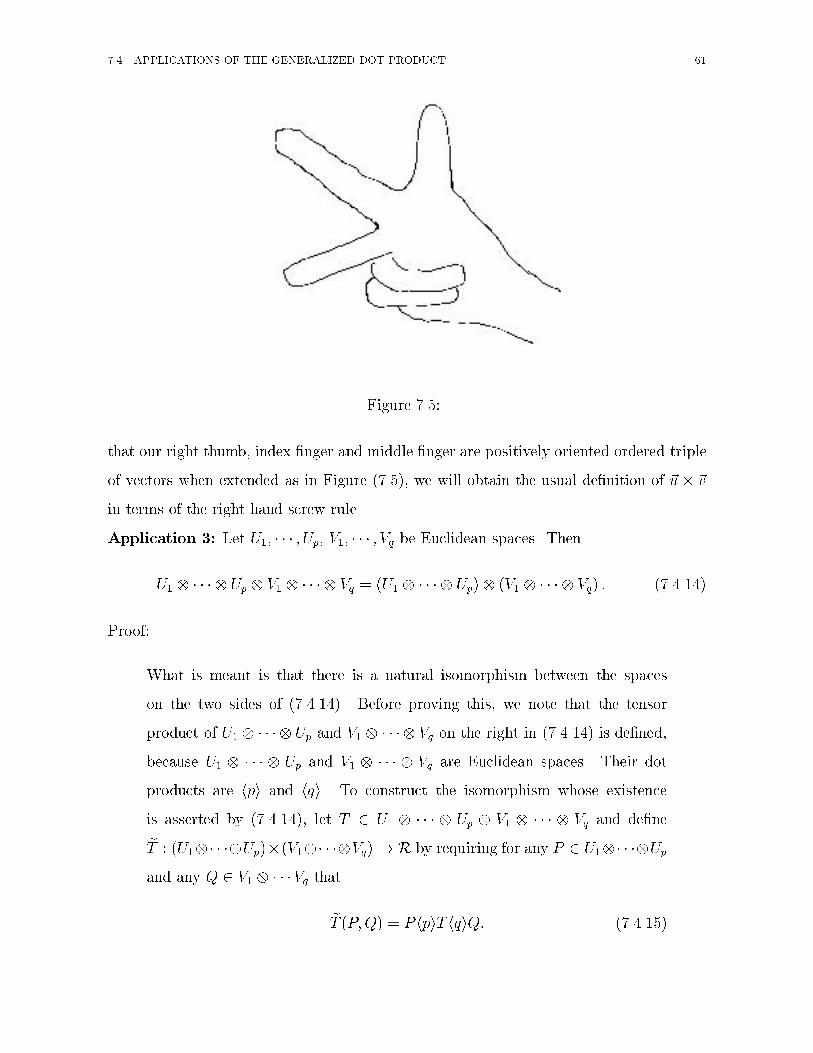
��� APPLICATIONS OF THE GENERALIZED DOT PRODUCT ��
Figure ����
that our right thumb� index �nger and middle �nger are positively oriented ordered triple
of vectors when extended as in Figure ������ we will obtain the usual de�nition of �u� �v
in terms of the right hand screw rule�
Application �� Let U�� � � � � Up� V�� � � � � Vq be Euclidean spaces� Then
U� � � � � � Up � V� � � � � � Vq � �U� � � � � � Up�� �V� � � � � � Vq� � ��������
Proof�
What is meant is that there is a natural isomorphism between the spaces
on the two sides of ��������� Before proving this� we note that the tensor
product of U� � � � � � Up and V� � � � � � Vq on the right in �������� is de�ned�
because U� � � � � � Up and V� � � � � � Vq are Euclidean spaces� Their dot
products are hpi and hqi� To construct the isomorphism whose existence
is asserted by ��������� let T � U� � � � � � Up � V� � � � � � Vq and de�neeT � �U��� � ��Up���V��� � ��Vq� R by requiring for any P � U��� � ��Up
and any Q � V� � � � �Vq that
eT �P�Q� � P hpiT hqiQ� ��������
�� CHAPTER � GENERALIZED DOT PRODUCTS
Then eT is bilinear� so eT � �U� � � � � � Up� � �V� � � � � � Vq�� From ���������g�ajTj� � aj eTj� so T � eT is a linear mapping of U� � � � � � Up � V� � � � � � Vq
into �U��� � ��Up���V��� � ��Vq�� We claim this mapping is bijective� To see
that it is injective� suppose T� � T� � U��� � ��Up�V��� � ��Vq and eT� � eT��Then for every P � U��� � ��Up and Q � V��� � ��Vq we have P hpiT�hqiQ �
P hpiT�hqiQ� so P hpi�T�hqiQ�T�hqiQ � � so P hpi��T��T��hqiQ� � �� Hence�
�T� � T��hqiQ � � for all Q � V� � � � � � Vq� Hence� T� � T� � �� To see
that T � eT is a surjection� suppose % � �U� � � � � � Up� � �V� � � � � � Vq��
De�ne T � U��� � ��Up�V��� � ��Vq by requiring T ��u�� � � � � �up� �v�� � � ��vq� �%��u� � � ��up� �v�� � � ��vq�� Then P hpiT hqiQ � %�P�Q� if P and Q are polyads�
Hence P hpiT hqiQ � %�P�Q� for all P � U�� � � ��Up and Q � V�� � � �� Vq�
By ��������� % � eT � Thus T � %� and the mapping T � eT is a surjection of
U� � � � � � Up � V� � � � � � Vq onto �U� � � � � � Up�� �V� � � � � � Vq��
Application �� Linear mappings as second order tensors�
De�nition ����� Suppose U and V are Euclidean vector spaces and L � L�U V ��
De�ne�
L� F�U � V R� by�
L ��u��v� � L��u� � �v� ��������
Then�
L ��� �v� and �
L ��u� �� are linear� so�
L� M�U � V R��
That is��
L� U � V� ��������
Thus� �������� can be written in the equivalent form
�u� �L ��v � L��u� � �v� ��������
For a �xed �u � U � �������� is true for all �v � V � Hence� since �u � �L and L��u� are both in
V � we have
�u� �L� L��u�� ��������
Let � � L�U V � U � V be de�ned by ��L� ��
L� If we know�
L� ��L�� we can
recover L from ��������� so � is an injection� We claim � is also a surjection� That is�

��� APPLICATIONS OF THE GENERALIZED DOT PRODUCT ��
every T � U�V is ��L� for at least one L � L�U V �� Suppose T is given and de�ne L
by L��u� � �u �T � Then �
L ��u��v� � �u� �L ��v � L��u� ��v � �u �T ��v � T ��u��v�� so T ��
L� ��L��
We claim that � � L�U V � U � V is also linear� If L�� � � � � Ln � L�U V � and
a�� � � � � an � R� we claim�
�aiLi�� ai�
Li � �������
The proof is this� for any �u � U and �v � V �
�u��
�aiLi� ��v � ��aiLi���u�� � �v � fai �Li��u��g � �v� ai �Li��u� � �v� � ai��u�
�
Li ��v�� �u �
�ai
�
Li
�� �v�
Thus ��
aiLi���u��v� � �ai�
L���u��v� for all �u � U � �v � V � Hence ��������
We have now shown that � is a linear bijection between the two vector spaces L�U V � and U � V � We can use � to regard any linear mapping L � U V as a tensor�
L� U � V and vice�versa� The process of taking linear combinations can be done either
to the tensors or to the linear mappings� so confusing tensors with linear mappings does
no harm to linear combinations�
Linear mappings can also be �multiplied� by composition� If K � L�U V � and
L � L�V W � then L � K � L�U W �� Our identi�cation of tensors with linear
mappings almost preserves this multiplication� We have
�
L �K��
K � �L � �������
The proof is simple� For any �u � U �
�u��
�L �K� � �L �K���u� � L �K��u��
� K��u�� �L� ��u � �K�� �L� �u � � �K� �L� by �������
Since this is true for all �u � U � corollary �������� gives ��������
If IU � U U is the identity operator on U �that is� IU��u� � �u for all �u � U� then for
any �u�� �u� � U ��
I U ��u�� �u�� � IU ��u�� � �u� � �u� � �u�� ������

�� CHAPTER � GENERALIZED DOT PRODUCTS
That is��
I U is what we have already called the identity tensor on U � see example �����
The origin of that name is now clear� And ������ can also be written
�u���
I U ��u� � �u� � �u�� ������
This is true for all �u� and �u� � U � so we have for any �u � U
�u� �I U��
I U ��u � �u� �������
If L � U V then L � IU � IV � L � L� It follows then from ������� that
�
I U ��
L��
L � �I V��
L � �������
Actually� a more general result is true� If U � V � W�� � � � � Wq are Euclidean spaces and
T � U �W� � � � � �Wq � V then
�
I U �T � T � �I V� T� �������
The proof follows the usual lines� Since all three expressions in ������� are linear in T � it
su!ces to prove ������� for polyads T � But for T a polyad� ������� follows immediately
from associativity and ��������
Thus��
I U acts like a multiplicative identity� Then some second order tensors can have
inverses�
De�nition ����� If L � L�U V � has an inverse L�� � L�V U�� then we de�ne��
L
���to be
�
L���
Thus� using �������� we conclude
�
L�� � �L��
I V ��
L ��
L����
I U � �������
Since the tensors in U � V and the linear mappings in L�U V � can be thought of
as essentially the same objects� any concept de�ned for one can be de�ned immediately
for the other� De�nition ���� is an example of this process� Other examples are below�
De�nition ����� If�
L� V � V then det�
L�� detL�

��� APPLICATIONS OF THE GENERALIZED DOT PRODUCT ��
From de�nition ���� and ����� it is apparent that for any�
L� V � V ��
L�� exists i�
det�
L �� ��
De�nition ����� If�
L� U � V then��
L
�T��
�
LT � Thus�
LT� V � U �
Here LT is the transpose of L � U V � as de�ned on page D��� From the de�nition
of LT we have��
L
�T��v� �u� �
�
LT ��v� �u� � LT ��v� � �u � �v � L��u� � L��u� � �v ��
L ��u��v�� Thus
�
LT� ����
L � �������
It is also true that for any ��u��v� � U � V � �v��
LT ��u ��
LT ��v � �u� ��
L ��u��v� � �u� �L ��v�Thus �v �
� �LT ��u� �u� �L
�� �� This is true for that for any �v � V so for all �u � U
�
LT ��u � �u� �L � �������
Similarly���v�
�
LT � �
L ��v�� �u � � for all �u � U so if �v � V
�v� �LT��
L ��v� �������
Application �� Linear mappings as higher order tensors�
Suppose U�� � � � � Up� V�� � � �Vq are Euclidean vector spaces and L � L�U�� � � ��Up V� � � � �Vq�� Both U� � � � � � Up and V� � � � � � Vq are Euclidean vectors spaces� with
dot products hpi and hqi� Therefore� L corresponds to a second order tensor�
L in �U� �� � � � Up� � �V� � � � � � Vq�� exactly as in ��������� That is if P � U� � � � � � Up and
Q � V� � � � � � Vq then�
L �P�Q� � L�P �hqiQ
or
P hqi �L hqiQ � L�P �hqiQ� �������
Here hpi and hqi are to be interpreted as the dot products on U��� � ��Up and V��� � ��Vq�and
�
L is a second order tensor in the space �U�� � � ��Up�� �V�� � � �� Vq�� which is the
tensor product of two Euclidean spaces�

�� CHAPTER � GENERALIZED DOT PRODUCTS
However� as we saw on page ����
L can also be interpreted as a tensor of order p � q
in U� � � � � � Up � V� � � � � � Vq� Equation ������� continues to hold� but now hpi andhqi are interpreted as generalized dot products� and
�
L� U� � � � � � Up � V� � � � � � Vq�
Therefore� the linear mappings L � L�U� � � � � � Up V� � � � � � Vq� can be viewed as
tensors�
L� U��� � ��Up�V��� � ��Vq� If we know L� we �nd�
L from ������� by taking
P and Q to be arbitrary polyads� If we know�
L� U� � � � � � Up � V� � � � � � Vq� then we
know it in �U� � � � � � Up�� �V� � � � � � Vq� so we �nd L by appealing to ��������� That
is� for any P � U� � � � � � Up�
L�P � � P hpi �L � ������
The generalization from application � to application � is particularly useful in con�
tinuum mechanics�

Chapter �
How to Rotate Tensors �and why
��� Tensor products of linear mappings
For j � f�� � � � � qg� suppose Vj andWj are Euclidean vector spaces and Lj � L�Vj Wj��
We would like to de�ne a linear mapping
L� � � � � � Lq � V� � � � � � Vq W� � � � � �Wq
by requiring that for any polyad �v� � � ��vq � V� � � � � � Vq we have
�L� � � � � � Lq� ��v� � � ��vq� � L� ��v�� � � �Lq ��vq� � �������
The lifting theorem will show that there is exactly one such L� � � � � � Lq� To �nd it� we
invoke that theorem� We de�ne
M � V� � � � � � Vq W� � � � � �Wq
by requiring for any ��v�� � � � � �vq� � V� � � � � � Vq that
M ��v�� � � � � �vq� � L���v�� � � �Lq��vq��
Since L�� � � � � Lq are linear� M is multilinear� so we can use the lifting theorem with M as
above and W � W��� � ��Wq� The picture is shown in ���� Then we de�ne L��� � ��Lq
to be the M provided by the lifting theorem� With this choice� L� � � � � � Lq is linear
and satis�es ��������
��

�� CHAPTER � HOW TO ROTATE TENSORS �AND WHY�
x
x
x x x x. . .
. . . x x
. . . V VM
W W1 q 1 q
V VM
1 q
Figure ����
Remark ���� Suppose��bj�� � � � � ��bj�nj
�is an ordered basis for Vj andQ � Qi����iq�b��i� � � ��bq�iq
� V� � � � � � Vq� Then
�L� � � � � � Lq� �Q� � Qi����iqhL�
��b��i�
�� � �Lq
��bq�iq
�i� ������
Proof�
L��� � ��Lq is linear� so �L��� � ��Lq��Q� � Qi����iqh�L� � � � � � Lq�
��b��i� � � ��bq�iq
�i�
Now use ��������
Remark ���� Suppose for j � f�� � � � � qg that Uj� Vj� Wj are Euclidean and Kj �L�Vj Wj� and Lj � L�Uj Vj�� Then
�K� � � � � �Kq� � �L� � � � � � Lq� � �K� � L��� � � � � �Kq � Lq� � ������
Proof�
We want to show for every P � U� � � � � � Uq that
��K� � � � � �Kq� � �L� � � � � � Lq�� �P � � ��K� � L��� � � � � �Kq � Lq�� �P ��
By linearity it su!ces to prove this when P is any polyad �u� � � ��uq� But
��K� � � � � �Kq� � �L� � � � � � Lq�� ��u� � � ��uq�� �K� � � � � �Kq� ��L� � � � � � Lq���u� � � ��uq��� �K� � � � � �Kq� �L���u�� � � �Lq��uq��
� K� �L��u���K� �L��u��� � � �Kq �Lq�uq�� ��K� � L����u�� ��K� � L����u���
� � � ��Kq � Lq���uq��
� ��K� � L��� � � � � �Kq � Lq�� ��u� � � ��uq��

���� TENSOR PRODUCTS OF LINEAR MAPPINGS ��
Another way to try to understand L� � � � � � Lq is to exhibit explicitly for any P �V� � � � � � Vq the tensor �L� � � � � � Lq��P � � W� � � � � � Wq by evaluating it at any
��w�� � � � � �wq� � W� � � � � �Wq� We have
Remark ���� Suppose that for j � f�� � � � � qg we have Lj � L�Vj Wj� for Euclidean
spaces Vj and Wj� Suppose P � V� � � � � � Vq and ��w�� � � � � �wq� � W� � � � � �Wq� Then
��L� � � � � � Lq��P �� ��w�� � � � � �wq� � PhLT� ��w��� � � � � LT
q ��wq�i� �������
Proof�
Both sides of this equation are linear in P � so it su!ces to prove the equation
when P is a polyad� P � �v� � � ��vq� In that case�
��L� � � � � � Lq��P �� ��w�� � � � � �wq� � �L���v�� � � �Lq��vq�� ��w�� � � � � �wq�
� �L���v�� � �w�� � � � �Lq��vq� � �wq�
�h�v� � LT
� ��w��i� � �
h�vq � LT
q ��wq�i
� PhLT� ��w��� � � � � LT
q ��wq�i�
Finally� it will be useful to understand how permutations a�ect tensor products of
mappings� To do this we need
Lemma ����� Suppose V�� � � � � Vq are Euclidean spaces� �vj � Vj for j � f�� � � � � qg� and� � Sq� Then
� ��v� � � ��vq� � �v������� � ��v���
�q�� �������
Proof�
From the de�nition ���������
�� ��v� � � ��vq����w������ � � � � �w���q�
�� ��v� � � ��vq� ��w�� � � � � �wq�
� ��v� � �w�� � � � ��vq � �wq�
���v����� � �w�����
�� � �
��v����q� � �w���q�
��
��v����� � � ��v���q�
� ��w������ � � � � �w���q�
�for any ��w�� � � � � �wq� � V� � � � � � Vq� QED�

� CHAPTER � HOW TO ROTATE TENSORS �AND WHY�
Now we can prove
Remark ����� For j � f�� � � � � qg� suppose Lj � L�Vj Wj�� and suppose � � Sq�
Then
� �L� � � � � � Lq� ��L����� � � � � � L���q�
��� �������
Proof�
The domain of L� � � � � � Lq is V� � � � � � Vq� We want to prove that if
P � V�� � � ��Vq then ���L�� � � ��Lq���P � � ��L������ � � ��L���q�����P ��
i�e�� ���L� � � � � � Lq���P � � �L����� � � � � � L���q����P �� Both sides of the
last equation are linear in P � so it su!ces to prove that equation when P is a
polyad� say P � �v� � � ��vq� In this case
� ��L� � � � � � Lq� ��v� � � ��vq�� � � �L���v�� � � �Lq��vq��
� L�����
��v�����
�� � �L���q�
��v���q�
�by �����
��L����� � � � � � L���q�
� ��v����� � � ��v���q�
��
�L����� � � � � � L���q�
��� ��v� � � ��vq�� by �����
QED�
Special Case�
Suppose V� � � � � � Vq � V and W� � � � � � Wq � W and L� � � � � � Lq � L� Then
we write L� � � � � � Lq as �qL� Then
�qL � L ��qV �qW � � �������
and �qL is de�ned by requiring for all ��v�� � � � � �vq� � xqV that
�qL��v� � � ��vq� � L��v�� � � �L��vq�� �������
If P � �qV � ������� leads to the �gure of speech that ��qL��P � is obtained by applying
L to P � �Really �qL is applied to P ��

���� APPLYING ROTATIONS AND REFLECTIONS TO TENSORS �
If K � L�V W � and L � L�U V � then from ������
��qK� � ��qL� � �q �K � L� � �������
If L � L�V W � and P � �qV and ��w�� � � � � �wq� � xqW then from �������
���qL��P �� ��w�� � � � � �wq� � PhLT ��w��� � � � � LT ��wq�
i� ��������
If L � L�V W � and � � Sq then from �������
���qL� � ��qL��� ��������
��� Applying rotations and re�ections to tensors
Recall that L � L�V V � is �orthogonal� if LT � L��� and �proper orthogonal� if also
detL � �� rather than ��� Recall the de�nitions on page D���
"�V � � set of all orthogonal operators on V
"��V � � set of all proper orthogonal operators on V�
Recall that according to corollary PP��� every proper orthogonal operator is a rotation�
As remarked on page PP��� if L is improper orthogonal �detL � ��� then L is the
product of a rotation and a re�ection�
If L is an orthogonal operator on V andQ � �qV � then two more facts about ��qL��Q�
make it even more reasonable to think of that tensor as the result of applying L to Q�
These facts are remark ����� and its corollary�
Remark ����� If L � "�V �� applying L to tensors over V preserves their generalized
dot products� More precisely suppose p� q� r are any non�negative integers� Suppose
P � �p�qV � R � �q�rV � and L � "�V �� Then
��p�rL��P hqiR� �h��p�qL��P �
ihqi
h��q�rL��R�
i� ������
Proof�

� CHAPTER � HOW TO ROTATE TENSORS �AND WHY�
Both sides of this equation are linear in P and R� so it su!ces to prove
the equation when P and R are polyads� say P � �u� � � ��up�x� � � ��xq and R �
�y� � � ��yq�v� � � ��vr � Then ��p�rL��P hqiR� � ��p�rL� ���x� � �y�� � � � ��xq � �yq��u� � � ��up�v� � � ��vr�� ��x� � �y�� � � � ��xq � �yq���p�rL���u� � � ��up�v� � � ��vr�� ��x� � �y�� � � � ��xq � �xq� �L��u�� � � �L��up�L��v�� � � �L��vr���
So far we have not used L � "�V �� Now we use it to set �x � �y � L��x� � L��y��Therefore the above polyad is ��p�rL��P hqiR� �
� �L��x�� � L��y��� � � � �L��xq� � L��yq�� �L��u�� � � �L��up�L��v�� � � �L��vr��� �L��u�� � � �L��up�L��x�� � � �L��xq�� hqi �L��y�� � � �L��yq�L��v�� � � �L��vr���
h��p�qL���u� � � ��up�x� � � ��xq�
ihqi
h��q�rL���y� � � ��yq�v� � � ��vr�
i�
h��p�qL��P �
ihqi
h��q�rL��R�
i�
QED
Corollary ���� The value of a rotated q�tensor at a rotated q�tuple of vectors is the
value of the original tensor at the original q�tuple of vectors� The same is true for re�ec�
tions� in general� if L � "�V � and Q � �qV and ��v� � � � � �vq� � xqV then
���qL� �Q�� �L ��v�� � � � � � L ��vq�� � Q ��v�� � � � � �vq� �
Proof�
���qL� �Q�� �L ��v�� � � � � � L ��vq��
� ���qL� �Q�� hqi �L ��v�� � L ��v�� � � �L ��vq��
� ���qL� �Q�� hqi ���qL� ��v��v� � � ��vq��� Qhqi ��v� � � ��vq� by remark �����
� Q ��v�� � � � � �vq� �

���� PHYSICAL APPLICATIONS �
��� Physical applications
Some physical properties of physical systems are tensors� For example� Ohm�s law in a
crystal says that if an electric �eld �E is applied� the resulting current density �J depends
linearly on �E� This means that there is a second�order tensor�
K such that �J � �E� �K�
This�
K is the �conductivity tensor� of the crystal� In a liquid� �J � �EK where K is a
scalar� so�
K� K�
I � but in a crystal all that can be said in general is that if there is
no magnetic �eld��
K is symmetric ��
KT��
K�� This is Onsager�s theorem for dissipative
thermodynamics�
A second example is an elastic crystal� As we will see later� its local state of deforma�
tion is described by a symmetric second order tensor�� � the strain tensor� Its local state
of stress is described by another symmetric second order tensor�
S � the stress tensor� For
small�� �i�e� k �
� k ������
S is a linear function of�� � so there is a tensor of fourth
order over ordinary �space� the elasticity tensor E� such that�
S��� hiE� Thermody�
namics assures that ���E � ���E � ������E � E� but E has no other symmetries
in general so the dimenson of the space of all possible elasticity tensors is �� �We will
discuss all this in detail later��
A third example is the second moment tensor�
M of a collection of mass points� If
there is a mass mv at position �rv for v � �� � � � � N � then
�
M ��NXv �
mv�rv�rv� ������
This is the underlying tensor from which the inertia tensor and gravitational second degree
harmonic tensor of a solid body are calculated�
If V is real �space and L � L�V V �� then �subjecting a physical system to the
mapping L� means that we move all the mass points �atoms� which make up the system�
so that a mass point which was originally at �rv is moved to the new location L��rv� � �rv��
L�
If L � "��V �� L subjects the body to a rigid rotation� If L � "�V � but detL � ��� Lsubjects the body to a rigid rotation and also a re�ection in some plane� If L � "�V �
but detL � � then L is the product of a rigid rotation and a symmetric linear operator�
The latter stretches the body by di�erent amounts in di�erent directions� If detL �� a

� CHAPTER � HOW TO ROTATE TENSORS �AND WHY�
H
F Br
Cl
Right Handed
H
F Cl
Br
Left Handed
Figure ���
re�ection also occurs�
It is actually possible to imagine subjecting a real body to a re�ection if we allow
ourselves to disassemble and reassemble the body atom�by�atom� For example� iceland
spar �calcite� crystals come in right�handed or left�handed version� Liquids can also be
re�ected� For most� re�ection has no e�ect because the distribution of molecules in the li�
quid has no preferred directions and the molecules either have no right� or left�handedness�
or the right� and left�handed versions are present in equal amounts� A liquid which is
a�ected by re�ection is bromochloro�uoromethane� CHFClBr� At one atmosphere of
pressure� it is liquid between �����C and ��C� the molecule is a tetrahedron with H� F�
Cl� Br at the four vertices and C at the center� It can come in two forms� left handed or
right handed� To re�ect a pot of left�handed CHFClBr means to replace it by a pot of
right�handed CHFClBr�
If we subject a system of mass points mv at positions �rv to the mapping L � L�V V �� where V is real �space� then the second moment tensor
�
M of that system �see �������
changes to ��L��
M�� To see this� note that the second moment tensor of the deformed

���� PHYSICAL APPLICATIONS �
system is
�
ML �NXv �
mvL ��rv�L ��rv� �NXv �
mv �� L ��rv�rv�
����L
�� NXv �
mv�rv�rv
�����L
�� �
M
��
If we subject a homogeneously stressed crystal to the mapping L� the stress tensor�
S in
that crystal will not change to ��L��
S�� Rather it will be determined by the elasticity
tensor E of the crystal� These examples show that it is not always obvious how to calculate
the e�ect of subjecting a physical system to a linear mapping L� Some tensor properties
of that system simply have L applied to them� and others do not�
The situation is much simpler if L � "�V �� To see this� suppose �b�� �b�� �b� is any basis
for real �space V � Suppose Q � �qV is a measurable tensor property of a particular
physical system� Then
Q � Qi����iq�bi��bi� � � ��biq � �����
�Measuring� Q means measuring the real numbers Qi����iq � Suppose we apply to the
physical system a mapping L � "�V �� The new physical system will have instead of
Q the tensor QL to describe that particular physical property� Suppose we apply L to
the apparatus we used to measure Qi����iq � and we use this mapped apparatus to measure
the contravariant components of QL relative to the basis L��b��� L��b��� L��b��� We assume
either that no gravity or electromagnetic �eld is present or� if they are� that they are
also mapped by L� Then the experiment on QL is identical to that on Q� except that it
has been rotated and possibly re�ected relative to the universe� As far as we know� the
univese does not care� the laws of nature are invariant under re�ection and rigid rotation�
The universe seems to be isotropic and without handedness� �As a matter of fact� a small
preference for one orientation or handedness exists in the weak nuclear force governing
��decay� Yang� Lee and Wu won Nobel prizes for this discovery� it has no measurable
e�ects at the macroscopic level of continuum mechanics in an old universe�� Therefore�
the numbers we read on our dials �or digital voltmeters� will be the same in the original
and mapped systems� That is� the contravariant components of QL relative to L��b���

� CHAPTER � HOW TO ROTATE TENSORS �AND WHY�
L��b��� L��b�� will be the same as the contravariant components of Q relative to �b�� �b�� �b��
Thus
QL � Qi����iqL��bi��� L��bi�� � � �L��biq �
� Qi����iq��qL���bi��bi� � � ��biq�� ��qL�
hQi����iq�bi�
�bi� � � ��biqi�
Therefore� if L � "�V � and the physical system is mapped by L� the new tensor property
QL is obtained by applying L to the original Q�
QL � ��qL��Q�� �����
A tensor property of a physical system rotates with that system� and is re�ected if the
system if re�ected�
�� Invariance groups
Sometimes� subjecting a physical system to certain rotations or re�ections will not a�ect
any of its measurable physical properties� For example� suppose I work all morning on
a cubic crystal of NaCl� While I am at lunch� you rotate it in such a way as simply to
permute its three crystal axes� When I return from lunch� I will be unable to detect that
anything has happened to the crystal� The same is true if you manange to work so fast
as to disassemble and reassemble the crystal so as to subject it to a re�ection along one
of its crystal axes while I am at lunch� If I was working not on NaCl but on a pot of
left�handed CHFCLBr before lunch� you can subject it to any rotation whatever� I will
not be able to detect the rotation when I return� However� if you re�ect it� I can detect
that now I have a pot of right�handed CHFClBr� For example� it will rotate the plane
of polarized light oppositely before and after lunch�
Let S be any physical system in real �space V � For any L � "�V �� let LS be the
physical system obtained by subjecting S to L� Let G�S� be the set of all members of
"�V � which� when applied to S� change none of the measurable properties of S� That is�L � ��V � is a member of G�S� if no measurement can distinguish between S and LS�
���� INVARIANCE GROUPS
These de�nitions have some simple but useful implications� Obviously
I � G�S� �������
where I is the identity operator on V � And if L�� L� � G�S�� then L�S is indistinguishable
from S� so L��L�S� is indistinguishable from S� Therefore
if L�� L� � G�S� then L� � L� � G�S�� ������
Finally� we claim
if L � G�S� then L�� � G�S�� ������
For LS and S are indistinguishable� Hence so are L���LS� and L��S� But L���LS�is S� so S and L��S are indistinguishable� Properties �������� ������� ������ show that
G�S�� is a subgroup of "�V �� It is called the invariance group of the physical system S�Examples of invariance groups are these�
Example ���� If S is water� G�S� � "�V ��
Example ���� If S is liquid� left�handed CHFClBr � G�S� � "��V ��
Example ��� If S is polycrystalline calcite� with the microcrystals randomly oriented�
and with equal numbers of right and left�handed microcrystals� and if we make only
measurements involving lengths � � microcrystal diameter �e�g� study only seismic
waves very long compared to the size of the microcrystals�� G�S� � "�V ��
Example ��� If in example ������ �& of the microcrystals are left handed and ��&
are right handed� G�S� � "��V ��
Example ��� If S is an NaCl crystal� G�S� is the �cubic group�� It is the group
of orthogonal operators which send into itself a cube centered on ��� If x�� x�� x� are
unit vectors parallel to the edges of the cube� G�S� consists of those L � "�V � such that
L� xi� � �i� x�i� for i � �� � � where � � S� and ��� ��� �� can be �� or �� independently�

� CHAPTER � HOW TO ROTATE TENSORS �AND WHY�
If Q � �qV describes some measurable property of physical system S� then clearly
��qL��Q� � Q for all L � G�S�� This fact limits the possible forms which Q can take�
and is therefore of physical interest� It leads us to introduce
De�nition ����� Let V be a Euclidean vector space� Let G be a subgroup of "�V ��
Then Iq�G� is the set of all Q � �qV such that
��qL� �Q� � Q for all L � G� �������
The set Iq�G� is called the space of q�th order tensors invariant under G� The tensors in
Iq�"�V �� are unchanged by any orthogonal operator� They are called �isotropic tensors��
The tensors in Iq�"��V �� are unchanged by any rotation� but may be changed by re�ec�
tions� They are called �skew isotropic tensors�� If G is the cubic group� the tensors in
Iq�G� are unchanged by any rotation or re�ection which is physically undetectable in an
NaCl crystal�
The following are simple consequences of de�nition ������
Corollary ����� Iq�G� is a subspace of �qV �
Proof�
Clearly Iq�G� � �qV � so all we need prove is that any linear combination of
members of Iq�G� is a member� If Q�� � � � � QN � Iq�G� and a�� � � � � aN � Rand L � G� then ��qL��Qi� � Qi� so ��qL��aiQi� � ai��qL��Qi� � aiQi
because �qL is linear�
Corollary ����� If G� � G� then Iq�G�� � Iq�G���
Proof�
If Q � Iq�G��� Q is unchanged by any L � G�� and then certainly by any
L � G�� Hence Q � Iq�G��� �The bigger the group G� the harder it is to be
unchanged by all its members��

���� INVARIANCE GROUPS �
Corollary ����� If Q � Iq�G�� and � � Sq then �Q � Iq�G��
Proof�
For any L � L�V V �� equation ������ gives ��qL� � � � � � ��qL�� Then
��qL���Q� � � ���qL��Q��� If Q � Iq�G� then for any L � G� ��qL��Q� � Q�
so ��qL���Q� � �Q� Hence �Q � Iq�G��
Corollary ����� If P � Ip�q�G� and R � Iq�r�G� then P hqiR � Ip�r�G��
Proof�
For any L � G� L � "�V �� so ��p�rL��P hqiR� � ���p�qL��P �� hqi ���q�rL��Q�� �
P hqiR �
Corollary ����� If Q � Iq�G� then the component array of Q is the same relative to
any two ordered orthonormal bases � x�� � � � � xn� and � x��� � � � � x�n� such that x�iL� xi� for
some L � G�
Proof�
For any Q � �qV �
Q � Qi����iq xi� � � � xiq � Q�i����iq
x�i� � � � x�iq � �������
For any L � L�V V ��
��qL� �Q� � Qi����iqL � xi�� � � �L� xiq�� �������
If Q � Iq�G� and x�i � L� xi� for some L � G� then ��qL��Q� � Q and
comparing ������� with ������� gives Qi����iq � Q�i����iq
�
Corollary ����� Suppose Q � �qV � Suppose V has one ordered orthonormal basis
� x�� � � � � xn� such that whenever L � G and x�i � L� xi�� then Q has the same component
array relative to � x�� � � � � xn� and � x��� � � � � x�n�� Then Q � Iq�G��
Proof�
Suppose L � G� Let x�i � L� xi�� By hypothesis Q�i����iq � Qi����iq � Comparing
�������� and ������� gives ��qL��Q� � Q� Since this is true for every L � G�Q � Iq�G��

�� CHAPTER � HOW TO ROTATE TENSORS �AND WHY�
�� Isotropic and skew isotropic tensors
De�nition ���� Let V be a Euclidean vector space� The tensors in Iq�"�V �� are
called �isotropic�� The tensors in Iq�"��V �� are called �skew isotropic��
Any tensor describing a measurable property of water� or of polycrystalline calcite with
randomly oriented microcrystals and equal numbers of left� and right�handed microcrys�
tals� is isotropic� Any tensor describing a property of left�handed liquid CHFClBr � or of
polycrystalline calcite with randomly oriented microcrystals and more of one handedness
than the other� is skew isotropic� Since "��V � � "�V �� corollary ������� implies
Iq�"�V �� � Iq�"��V ��� �������
That is� every isotropic tensor is skew isotropic�
By corollaries ����� and ������ a tensor is isotropic i� it has the same array of
components relative to every orthonormal basis for V �
Suppose �V�A� is an oriented Euclidean space� By corollary ������ a tensor is skew
isotropic if it has the same array of components relative to every positively oriented
orthonormal basis for V � Also� it is skew isotropic if it has the same array of components
relative to every negatively oriented orthonormal basis for V � If a tensor is skew isotropic�
by corollary ����� it has the same array of components relative to every positively oriented
orthonormal basis� and the same array relative to every negatively oriented orthonormal
basis� The two arrays need not be the same �indeed� if they are� the tensor is isotropic��
Example ����� The identity tensor�
I is isotropic� For� relative to any orthonormal
basis � x�� � � � � xn� for V � Iij ��
I � xi� xj� � xi � xj � �ij�
Example ����� If A is a unimodular alternating tensor� A is skew isotropic but not
isotropic� For as we saw on page �� A has the same component array relative to every
positively oriented orthonormal basis� but its component array changes sign for negatively
oriented bases�

���� ISOTROPIC AND SKEW ISOTROPIC TENSORS ��
Example ����� By corollary ������
I�
I is isotropic� So is�
I�
I�
I ��
I�
I�
I�
I � etc� By
corollary ���� � every permutation of these tensors is isotropic� By corollary ������
every linear combination of such permuted tensors is isotropic�
Example ����� All the tensors in example ����� are skew isotropic� By corollary
����� so are�
IA��
I�
IA��
I�
I�
IA� etc� By corollary ����� so are all permutations of these
tensors� By corollary ������ so is every linear combination of such permuted tensors� We
gain nothing new by using more than one factor A� The polar identity ����� shows that
if n � dimV then AA is a linear combination of n� permutations of�
I�
I � � � �I �with n
factors�
I ��
On p� �� of his book �The Classical Groups� �Princeton� ������ Hermann Weyl shows
that there are no isotropic tensors except those listed in example ������ and no skew
isotropic tensors except those listed in example ������ Note the corollary that all nonzero
isotropic tensors are of even order� We cannot consider Weyl�s general proof� but we will
discuss in detail the tensors of orders q � �� �� � � �� which are of particular interest in
continuum mechanics� We assume dimV � �
q � � Tensors of order � are scalars� They are una�ected by any orthogonal transform�
ation� so are isotropic and therefore also skew isotropic�
q � � If dimV � � the only skew isotropic tensor of order � is ��� Therefore the only
isotropic tensor of order � is ���
Proof�
Tensors of order � are vectors� We are claiming that if dimV � then
the only vector which is una�ected by all rotations is the zero vector�
A formal proof of this intuitively obvious fact is as follows� Suppose
�v � I��"��V ��� Let x and y be any two unit vectors� Each is the �rst
vector of a positively oriented ordered orthonormal basis �pooob�� so by
corollary ������ �v� x� � �v� y�� That is �v � x � �v � y for any two unit vectors

�� CHAPTER � HOW TO ROTATE TENSORS �AND WHY�
x and y� If dimV � � we can always �nd a y such that �v � y � �� Then
�v � x � � for all x� so �v � ���
q �
I��"�V �� � spf�I g ������
I��"��V �� � spf�I g if dimV � ������
I��"��V �� � spf�I � Ag if dimV � and
A is any nonzero member of ��V� �������
Proof�
The containments � have all been established in examples ����� and
������ so we need prove only � in ������ ����� ������� In all these cases�
suppose T � I��"��V ��� If x and y are any unit vectors� each is the
�rst vector of an ordered orthonormal basis �oob�� and by changing the
sign of one later basis vector� if necessary� we can assume that these oob�s
have the same orientation� Therefore T � x� x� � T � y� y� because T has
the same component array relative to all oobs with the same orientation�
Thus there is a scalar aT such that
T � x� x� � aT for every unit vector x� �������
If f x� yg is orthonormal� � x� y� is the �rst pair of vectors in an oob� Re�
placing � x� y� by � y�� x� in that oob gives a second oob with the same
orientation� Hence� T � x� y� � T � y�� x� � �T � y� x��
T � x� y� � �T � y� x� if f x� yg is orthonormal � �������
When dimV � � choose an oob � x�� x�� and let a � aT � b � T � x�� x��
�A� x�� x��� Then relative to this oob� Tij � a�ij � bA� x�� x���ij � �a�
I
�bA�ij� so T � a�
I �bA� and ������� is proved� To treat ������ ������ let

���� ISOTROPIC AND SKEW ISOTROPIC TENSORS ��
� x� y� be orthonormal� Both � x� y� and � y� x� are the �rst pair of vectors
in an oob� so if T � I��"�V ���
T � x� y� � T � y� x� if f x� yg is orthonormal� �������
If dimV � � both � x� y� and � y� x� are �rst pairs in oobs with the same
orientation� namely � x� y� x�� � � � � xn� and � y� x�� x�� x�� � � � � xn�� If T �I�"��V ��� we again have ������ In either case we have ������� and �������
so
T � x� y� � � if f x� yg is orthonormal� �������
Now let � x�� � � � � xn� be an oob� By ������� and �������� relative to this
oob we have Tij � aT �ij� so T � aT�
I � QED
q �
I��"�V �� � f�g �������
I��" � �V �� � f�g if dimV �� ��������
I��"��V �� � spfAg if dimV � and A �� �� A � ��V� ��������
Proof�
If dimV is even� let � x�� � � � � xn� be an oob for V � Then �� x�� � � � �� xn�is another oob with the same orientation� Then if T � I��"��V ���
T � xi� xj� xk� � T �� xi�� xj�� xk� � �T � xi� xj� xk� � � so Tijk � � �
If dimV is odd and dimV � �� let � x� y� z� be any ordered orthonor�
mal sequence� It is the �rst triple of an oob � x� y� z� x�� � � � � xn� and
�� x� y� z�� x�� x�� � � � xn� is an oob with the same orientation� so
T � x� y� z� � T �� x� y� z� � �T � x� y� z� � �� Similarly� T � x� y� y� �
�T � x� y� y� � � and T � x� x� x� �� �T � x� x� x� � �� Thus if x�� x�� x�
are orthonormal� T � xi� xj� xk� � � for fi� j� kg � f�� � � g� This com�
ment applies to any three vectors from an arbitrary oob for V � so Tijk � �

�� CHAPTER � HOW TO ROTATE TENSORS �AND WHY�
for fi� j� kg � f�� � � � � ng relative to any oob� and T � �� Finally� sup�
pose dimV � � If f x� yg is orthonormal� � x� y� is the �rst pair of an
oob � x� y� z�� and the oob �� x� y�� z� has the same orientation� Thus
T � x� y� y� � T �� x� y� y� � �T � x� y� y� � �� Similarly T � y� x� y� � � and
T � y� y� x� � �� Also T � x� x� x� � T �� x�� x�� x� � �T � x� x� x� � ��
Thus if T � I��"��V ��
T � x� x� x� � � for every unit vector x �������
T � x� y� y� � T � y� x� y� � T � y� y� x� if f x� yg is orthonormal� �������
Finally� if � x� y� z� is an oob� then the following are oobs with the same
orientation� � y� z� x� � � z� x� y� � � y� x�� z� � � x�� z� y� � �� z� y� x� � Then
if T � I��"��V ��
T � x� y� z� � T � y� z� x� � T � z� x� y� � �T � y� x� z� � �T � x� z� y� � �T � z� y� x���������
if f x� y� zg is orthonormal� Let � x�� x�� x�� be an oob for V � Let c �
T � x�� x�� x���A� x�� x�� x��� Then ������ � ����� � ������� imply Tijk �
cA� x�� x�� x���ijk � cAijk so T � cA� QED�
Note that in all the foregoing arguments� only mutually � vectors were used� These
arguments remain valid if G is the cubic group and T � Iq�G� with q � �� � and
we work only with unit vectors and oobs in the crystal axis directions� Therefore
the conclusions apply to tensors of orders �� � known only to be invariant under
the cubic group of Na Cl� For example� it follows that the conductivity tensor�
K
of Na Cl must have the form K�
I � In Na Cl� Ohm�s law �J � �E� �K reduces to the
isotropic form �J � �EK� even though an NaCl crystal is not isotropic�
q � �
I��"�V �� � sp��
I�
I � ���
I�
I � ����
I�
I
���������

���� ISOTROPIC AND SKEW ISOTROPIC TENSORS ��
I��"��V �� � ��if dimV �� f� �g ��������
I��"��V �� � sp��
I�
I � ���
I�
I � ����
I�
I � A�
if dimV � � ��������
I��"��V �� � spf�I�I � �� �I�I � ��� �I�I ��
IA� ���
IA� ����
IA�
A�
I � ��A�
I � ���A�
I g if dimV � � ��������
Here A is any nonzero alternating tensor� A � �nV with n � dimV �
Proof�
The containments � have all been established in examples ����� and ������
so we need prove only �� We consider only �������� �������� and leave ��������
������� to the reader with Sitz�eisch� Therefore we assume T � I��"��V ���
and if dimV � f� �g we assume T � I��"�V ��� If dimV � �� then any four
orthonormal vectors � w� x� y� z� are the �rst four vectors of and oob for V � say
� w� x� y� z� x�� � � � � xn�� The vectors �� w� x� y� z� are the �rst four vectors of
an oob with the same orientation� namely �� w� x� y� z�� x�� x�� � � � � xn�� SinceT � I��"��V ��� T has the same component array relative to both oob�s� so
T � w� x� y� z� � T �� w� x� y� z� � �T � w� x� y� z�� Thus for dimV � ��
T � w� x� y� z� � � if f w� x� y� z�g is orthonormal� ��������
This result is also vacuously true for dimV � � because then we cannot �nd
four orthonormal vectors in V �
Next� suppose dimV � and f x� y� zg is orthonormal� Then f x� y� zg and
�� x� y�� z� are both the �rst triple in oobs with the same orientation� so
T � x� y� z� z� � T �� x� y�� z�� z� � �T � x� y� z� z� � �� Similarly� if f x� y� zg isorthonormal
T � x� y� z� z� � T � x� z� y� z� � T � x� z� z� y�
� T � z� x� y� z� � T � z� x� z� y� � T � z� z� x� y� � �� �������
�� CHAPTER � HOW TO ROTATE TENSORS �AND WHY�
Equations ������� are vacuously true if dimV � because then we cannot
�nd three orthonormal vectors in V �
Next� suppose f x� yg is orthonormal� Then � x� y� and �� x� y� are the �rst pairsin oobs� and if dimV � we may assume these oobs to have the same orient�
ation� say � x� y� x�� � � � xn� and �� x� y�� x�� x�� � � � xn�� Then T � x� y� y� y� �
T �� x� y� y� y� � �T � x� y� y� y� � �� Similarly
T � x� y� y� y� � T � y� x� y� y�
� T � y� y� x� y� � T � y� y� y� x� � � if f x� yg orthonormal��������
Next� suppose that f x� yg and f x�� y�g are both orthonormal� Each pair � x� y�
and f x�� y�g is the �rst pair in an oob� so if T � I��"�V �� then T � x� x� y� y� �
T � x�� x�� y�� y��� If dimV � � then � x� y� and � x�� y�� are �rst pairs in oobs with
the same orientation� say � x� y� x� � � � � xn� and � x�� y��� x�� x�� � � � � xn�� Then in
that case also� T � x� x� y� y� � T � x�� x�� y�� y��� In either case� there is a scalar
T depending only on T such that
T � x� x� y� y� � T if f x� yg is orthonormal� ������
Similarly� there are scalars uT and vT such that
T � x� y� x� y� � uT if f x� yg is orthonormal� ������
T � x� y� y� x� � vT if f x� yg is orthonormal� �������
Finally� if x and y are unit vectors� each is the �rst member of an oob� and
the two oobs can have the same orientation� so T � x� x� x� x� � T � y� y� y� y��
Therefore� there is a scalar �T depending only on T such that
T � x� x� x� x� � �T for every unit vector x� �������
Then tensor�
I�
I satis�es ���������������� with � � �� � �� u � �� v � ��
The tensor ���
I�
I satis�es ���������������� with � � � � � � � u � ��

���� ISOTROPIC AND SKEW ISOTROPIC TENSORS �
v � �� The tensor ����
I�
I satis�es ���������������� with � � � � � � �
u � �� v � �� Therefore� the tensor
S � T � T�
I�
I �uT ���
I�
I �vT ����
I�
I �������
satis�es ���������������� with �S � �T �T �uT �vT and S � uS � vS � ��
Now let � x� y� be orthonormal in V and let � x� y� x�� � � � � xn� be an oob for V �
Then � x�� y�� x�� � � � � xn� is an oob with the same orientation if we take
x� � x cos � � y sin �� y� � � x sin � � y cos ��
To see this� let A � �nV � A �� �� Then
A� x�� y�� x�� � � � xn� � A� x cos � � y sin ��� x sin � � y cos �� x�� � � � � xn�� � cos � sin �A� x� x� x�� � � � � xn� � cos� �A� x� y� x�� � � � � xn�� sin�A� y� x� x�� � � � � xn� � sin � cos �A� y� y� x�� � � � � xn�
��cos� � � sin� �
�A� x� y� x�� � � � � xn� � A� x� y� x�� � � � � xn��
But if � x� y� x�� � � � � xn� and � x�� y�� x�� � � � � xn� have the same orientation and
S � I��"��V ��� the S� x� x� x� x� � S� x�� x�� x�� x��� The S of ������� is a linear
combination of members of I��"��V ��� so it is in I��"��V ��� In addition� S
satis�es ���������������� with S � uS � vS � �� Therefore
S� x� x� x� x� � S� x�� x�� x�� x��
� S� x cos � � y sin ��
x cos � � y sin �� x cos � � y sin �� x cos � � y sin ��
� cos� �S� x� x� x� x� � sin� �S� y� y� y� y� �������
since all other �� terms in the multilinear expansion of S vanish� Thus �S �
�cos� � � sin� ���S� It is possible to choose � so that cos� � � sin� � �� ��
Therefore �S � �� Therefore S � �� Therefore
T � T�
I�
I �uT ���
I�
I �vT ����
I�
I � �������

�� CHAPTER � HOW TO ROTATE TENSORS �AND WHY�
This completes the proofs of �������� and ���������
Notice that the proof of ������� works equally well if all the unit vectors are
parallel to the crystal axes of an Na Cl crystal� Only ������� fails� But if
x� y� z are crystal axes� then S � �S� x x x x� y y y y� z z z z�� Therefore� we have
proved that if T is invariant under the cubic group we can write
T � �S � x x x x� y y y y � z z z z�
� T�
I�
I �uT ���
I�
I �vT ����
I�
I � �������
where �S � �T � T � uT � vT �
Chapter �
Di�erential Calculus of Tensors
��� Limits in Euclidean vector spaces
De�nition ���� Let U be a Euclidean vector space� Let �u � U � Let t � R� t � �� We
de�ne three sets�
i� B��u� t� �� f�u� � �u� � U and k�u� � �uk tg
ii� B��u� t� �� f�u� � �u� � U and k�u� � �uk � tg
iii� 'B��u� t� �� f�u� � �u� � U and k�u� � �uk � tg �
B��u� t� � B��u� t� and 'B��u� t� are called� respectively� the open ball� the sphere� and the
closed ball centered at �u with radius t� See �gure ���
De�nition ���� A subset D of Euclidean space U is �open� if every point in D is the
center of a ball lying entirely in D� That is� if �u � D then �� � � � B��u� �� � D� See
�gure ���
De�nition ����� Suppose U and V are Euclidean vector spaces� D � U � �f � D V �
�u� � D and �v� � V � We say that lim�u��u��f��u� � �v�� or� equivalently �f��u� �v�� as �u �u�
if for every � � � there is a ���� � � such that whenever �u � D and � k�u� �u�k ����
then kf��u�� �v�k ��
��

�� CHAPTER � DIFFERENTIAL CALCULUS OF TENSORS
u
t
B(u, t)
B(u, t) ∂
Figure ����
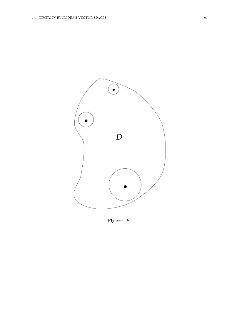
���� LIMITS IN EUCLIDEAN VECTOR SPACES ��
D
.
.
.
Figure ���
�� CHAPTER � DIFFERENTIAL CALCULUS OF TENSORS
De�nition ����� If �f��u�� � �v� in de�nition ����� then �f is �continuous at �u���
De�nition ����� If x and y are real numbers� denote the algebraically smaller of them
by x � y �read �x meet y�� and the algebraically larger by x � y �read �x join y��� Thus
� � � � �� � � � � �� ���� � � � ��� ���� � � � ��
Corollary ����� Suppose U and V are Euclidean vector spaces� D � U and f � D V �
Suppose �u� � D� �v� � V and �f��u� �v� as �u �u�� Then if �u � D and k�u� �u�k �����
we have
kf��u�k � � k�v�k�
Proof�
If �u � D and k�u��u�k ����� then kf��u���v�k � so k�f��u�k � k�f��u���v���v�k � kf��u�� �v�k� k�v�k � � k�v�k�
Corollary ���� Suppose U and V are Euclidean vector spaces� D � U � �f � D V �
�f � � D V � �u� � D� �v� and �v�� � V � Suppose that �f��u� �v� and �f ���u� �v �� as �u �u��
Then ��f � �f ����u� �v� � �v �� as �u �u��
Proof�
For any given � � � we must �nd a ������ � � such that �u � D and k�u��u�k ������ implies k�f � f ����u���v���v ��k �� By hypothesis� there are ����� � �
and ������ � � such that if �u � D then
k�f��u�� �v�k �� if k�u� �u�k ����� �������
k�f ���u�� �v ��k �� if k�u� �u�k � ������ ������
Let ������ � ����� � ������� If k�u � �u�k ������� then both ������� and
������ are true� so k��f � �f ����u� � �v� � �v ��k � k�f��u� � �v� � �f ���u� � �v ��k �k�f��u�� �v�k� k�f ���u�� �v ��k � �� � �� � �� QED�

���� LIMITS IN EUCLIDEAN VECTOR SPACES ��
Corollary ���� Suppose U � V � W � X are Euclidean vector spaces and D � U and
R � D V � W and T � D W � X� De�ne R � T � D V � X by requiring
�R � T ���u� � R��u� � T ��u� for each �u � D� Suppose �u� � D and as �u �u� we have
R��u� R� and T ��u� T�� Then �R � T ���u� R� � T��
Proof�
Choose � � �� We must �nd ���� � � such that if �u � D and k�u� �u�k ����
then k�R � T ���u�� R� � T�k �� We note
�R � T ���u�� R� � T� � R��u� � T ��u�� R� � T�� R��u� � T ��u�� R��u� � T� �R��u� � T� �R� � T�� R��u� � �T ��u�� T�� � �R��u�� R�� � T��
Thus
k�R � T ���u�� R� � T�k � kR��u� � �T ��u�� T�� k� k �R��u��R�� � T�k�
The generalized Schwarz inequality� remark ����� gives
kR��u� � �T ��u�� T�� k � kR��u�kkT ��u�� T�kk�R��u�� R�� � T�k � kR��u��R�kkT�k�
Thus if �u � D
k�R � T ���u�� R� � T�k � kR��u�kkT ��u�� T�k� kR��u��R�kkT�k� ������
Now if �u � D and�����������������
if k�u� �u�k �R��� then kR��u�k � � kR�k �see corollary ������
if k�u� �u�k �T�
����kR�k�
�then kT ��u�� T�k �
���kR�k�
if k�u� �u�k �R�
����kT�k�
�then kR��u��R�k �
���kT�k��
�������

�� CHAPTER � DIFFERENTIAL CALCULUS OF TENSORS
Take ���� � �R��� � �T�
����kR�k�
�� �R
��
���kT�k�
�� Then if k�u� �u�k �����
we have all three of �������� so by �������
k�R � T ���u�� R� � T�k �� � kR�k� �
�� � kR�k� �kT�k�
�� � kT�k� ��
QED�
Corollary ���� Suppose U and V are Euclidean vector spaces� and D � U � and
�u� � D and �v� � V � Suppose �f � D V is de�ned by �f��u� � �v� for all �u � D� Then
�f��u� �v� as �u �u��
Proof�
Obvious from de�nition ������
Corollary ����� Suppose U and V are Euclidean vector spaces� and D � U � and
�u� � D and �v� � V � Suppose �f � D V �
i� If �f��u� �v� as �u �u�� then �bi � �f��u� �bi � �v� as �u �u�� for any basis ��b�� � � � ��bn� of
V � with dual basis ��b�� � � � ��bn��
ii� If there is one basis for V � ��b�� � � � ��bn�� such that �bi � �f��u� �bi � �v� as �u �u�� then
�f��u� �v� as �u �u��
Proof�
Regard �bi as a function whose domain is D and whose value is �bi for each
�u � D� Then i� follows from corollaries ����� and ������ And ii� follows
from corollaries ����� � ������ and ������
Notice that the ranges of our functions can lie in tensor spaces since these are Euclidean
vector spaces� The corollaries all apply verbatim� The dot products are� of course�
the generalized dot products used to make tensor spaces Euclidean� The only corollary
which perhaps deserves comment is ������ It now reads thus� Suppose U � V�� � � � � VW�� � � � �Ws� X�� � � � � Xt are Euclidean vector spaces� and D � U and R � D V� �

���� GRADIENTS� DEFINITION AND SIMPLE PROPERTIES ��
� � � � Vr �W� � � � � �Ws and T � D W� � � � � �Ws �X� � � � � �Xt� De�ne RhsiT �
D V� � � � � � Vr � X� � � � � � Xt by requiring �RhsiT ���u� � R��u�hsiT ��u� for each
�u � D� Suppose �u� � D and as �u �u� we have R��u� R� and T ��u� T�� Then
�RhsiT ���u� R�hsiT��
��� Gradients� De�nition and simple properties
De�nition ����� We de�ne the �dot product� of two real numbers to be their ordinary
arithmetic product� With this de�nition� R is a one�dimensional Euclidean vector space�
and it has two orthonormal bases� f�g and f��g� which we write as � and � � when
thinking of R as a Euclidean space� When we think of a real number as a vector� we
write it with an arrow� like �� Thus � � �� and � � � � � � ���
De�nition ����� Suppose U and V are Euclidean vector spaces� D is an open subset
of U � �f � D V � and �u � D� A linear mapping L � U V is a �gradient mapping for �f
at �u � if there is a function �R � U V �which may depend on �f and �u and L � such that
a� lim�h���
�R��h� � ��� and
b� �f��u� �h� � �f��u� � L��h� � k�hk�R��h� for any�h � U such that �u� �h � D� ������
Remark ����� �f has at most one gradient mapping at �u�
Proof�
If L� and L� are both gradient mappings for �f at �u then whenever �u��h � D
we have
�f��u� �h� � �f��u� � L���h� � k�hk�R���h�
� �f��u� � L���h� � k�hk�R���h��
Therefore if �u� �h � D�
L���h� � k�hk�R���h� � L���h� � k�hk�R���h�� �����

�� CHAPTER � DIFFERENTIAL CALCULUS OF TENSORS
Now D is open� so there is an � � � such that if k�hk � then �u � �h � D�
Let �k be any vector in U � and let t be any nonnegative real number� Then
kt�kk � as long as � � t ��k�kk� Therefore� if t is in this range� ��� is
true for �h � t�k� That is
L��t�k� � kt�kk�R��t�k� � L��t�k� � ktkkR��t�k��
But Li�t�k� � tLi�k� and kt�kk � tk�kk� so if t � �
L���k� � k�kk�R��t�k� � L���k� � k�kk�R��t�k�� �����
This is true for all t in � t ��k�kk� Let t �� and both �R��t�k� �� and
�R��t�k� ��� Therefore L���k� � L���k�� Since this is true for all k � U � we
have L� � L�� QED
De�nition ����� In de�nition ���� if �f � D V has a gradient mapping L at �u�
then �f is �di�erentiable at �u �� and �R is the �remainder function for �f at �u �� The tensor�
L� U � V is called the �gradient tensor of f at �u � or the �gradient of �f at �u �� It is
written �r�f��u�� Since L��h� � �h� �L� we can rewrite ��� as
a� lim�h���
�R��h� � �� and
b� �f��u� �h� � �f��u� � �h �h�r�f��u�
i� k�hk�R��h� if �u� �h � D� ������
Remark ����� Suppose U and V are Euclidean vector spaces� D is an open subset of
U � �u � D� and �f � D V � Suppose there is a tensor�
L� U�V and a function �R � D V
with these properties�
a� lim�h���
�R��h� � �� and
b� �f��u� �h� � �f��u� � �h � L� k�hk�R��h� if �u� �h � D� ������
Then �f is di�erentiable at �u� its gradient tensor at �u is�
L� and its remainder function at
�u is �R�
Proof�

���� GRADIENTS� DEFINITION AND SIMPLE PROPERTIES �
�h � �h� �L is a linear mapping L� so ������ � ������� Therefore �f is di�er�
entiable� By Remark ����� L is the gradient mapping for �f at �u� so�
L is the
gradient tensor� Then the �R�s in �����b� and �����b� must be the same�
Example ����� Suppose �f � D V is constant� Then �f is di�erentiable at every
�u � D and �r�f��u� ����
Proof�
The hypotheses of remark ���� are satis�ed with�
L����
�
R ��h� � ���
Example ����� Suppose �f � D U is the identity mapping on D� i�e� �f��u� � �u for
all �u � D� Then �f is di�erentiable everywhere in D� and for each �u � D� �r�f��u� ��
I U �
the identity tensor on U � �This result is often abbreviated �r�u ��
I U ��
Proof�
The hypotheses of remark ���� are satis�ed with�
L��
I U � �R��h� � ���
Example ����� Suppose U and V are Euclidean spaces� D is an open subset of U and�
T is a �xed tensor in U � V � Suppose �f � D V is de�ned by �f��u� � �u� �T for every
�u � D� Then at every �u � D� �f is di�erentiable and �r�f��u� ��
T � �Often abbreviated
�r��u� �T � ��
T ��
Proof�
The hypotheses of remark ���� are satis�ed with�
L��
T � �R��h� � ���
Example ���� Suppose that for i � f�� � � � � ng we have ai � R and �fi � D V �
Suppose all the �fi are di�erentiable at �u � D� Then so is ai �fi � D V � and �r�ai �fi���u� �ai��r�fi���u��
Proof�
Each �fi satis�es equation ������� so the hypotheses of remark ���� are sat�
is�ed for ai �fi with�
L� ai��r�fi��u�� and �R��h� � ai �Ri��h��

�� CHAPTER � DIFFERENTIAL CALCULUS OF TENSORS
Example ���� Suppose thatD is an open subset of Euclidean space U and f � D R�
In elementary calculus classes� f is de�ned to be di�erentiable at �u � D if there is a vector
�L � U and a function R � U R such that
a� lim�h���
R��h� � � and
b� f��u� �h� � f��u� � �h � �L� k�hkR��h� if �u� �h � D� ������
The vector �L is called the gradient of f at �u� written �rf��u�� If we think of R as a one�
dimensional Euclidean space� then we can think of f as a vector�valued function �f � f �
�the vector is one dimensional�� The scalar valued function f is di�erentiable in the sense
of equations ������ i� �f � f � is di�erentiable in the sense of equation ������� and then
�r�f��u� � �rf��u� �� �rf��u� � �r�f��u� � �� ������
Proof�
To obtain ������ from ������� multiply all terms in ������ on the right by ��
To obtain ������ from ������ dot � on the right in all terms in ������� Here
clearly�
L� �L � � �rf��u� ��
Example ���� Suppose D is an open subset of R� regarded as a one�dimensional
Euclidean space� Suppose �f � D V has an ordinary derivative at u � D �we will write
this derivative as u �f�u� rather than d�f�du� for reasons made clear later�� Then �f is
di�erentiable at �u and
�r�f�u� � �u �f�u�� ������
Proof�
By hypothesis� limh��
��fu�h���fu�
h
�� u �f�u�� De�ne �R�h� � � if h � � and
for h �� � then
�R�h� �h
jhj
��� �f�u� h�� �f�u�
h� u �f�u�
� �

���� GRADIENTS� DEFINITION AND SIMPLE PROPERTIES ��
Then limh���R�h� � ��� and
�f�u� h� � �f�u� � hu �f�u� � jhj�R�h�� ������
But h � �h � � so hu �f��u� � �h � �u �f�u�� Also jhj � k�hk� Therefore ������ is
������ with�
L� �u �f�u��
Example ����� Suppose f � D R and �g � D V are di�erentiable at �u � D� Then
so is the product function f�g � D V � and
�r�f�g���u� �h�rf��u�
i�g��u� � f��u�
h�r�g��u�
i� �������
Proof�
By hypothesis� if �u� �h � D then
f��u� �h� � f��u� � �h � �rf��u� � k�hkRf��h
�g��u� �h� � �g��u� � �h � �r�g��u� � k�hkRg��h��
Multiplying these two equations gives
f��u� �h��g��u� �h� � f��u��g��u� � �h �hf��r�g� � ��rf��g
i� k�hk�Rfg��h� �������
where� by de�nition�
�Rfg��h� � Rf ��h�h�g��u� � �h � �r�g��u�
i��Rg��h�
hf��u� � �h � �rf��u�
i� k�hkRf ��h��Rg��h�
�h�h � �rf��u�
i h�h � �r�g��u�
i�k�hk�
As �h ��� the three terms in �Rfg� which involve Rf or �Rg� obviously �� So does the last term� because by Schwarz�s inequality its length is �k�hkk�rf��u�kk�r�g��u�k� Therefore remark ���� can be applied to ��������
QED�

��� CHAPTER � DIFFERENTIAL CALCULUS OF TENSORS
Example ����� The Chain Rule� Suppose U � V � W are Euclidean vector spaces Df
is an open subset of U � Dg is an open subset of V � and f � Df Dg and g � Dg W �
Suppose �u � Df and �v � �f��u�� Suppose �f is di�erentiable at �u and �g is di�erentiable at
�v� Then their composition� �g � �f � Df W � is di�erentiable at �u and
�r��g � �f���u� � �r�f��u� � �r�g��v�� ������
Proof�
Let�
Lf� �r�f��u� and�
Lg� �r�g��v�� Let �Rf and �Rg be the remainder functions
for �f at �u and �g at �v� Then �Rf ��h� �� as �h ��� and �Rg��k� �� as �k ���
and
�f��u� �h� � �f��u� � �h� �Lf �k�hk�Rf ��h� if �u� �h � Df � ������
�g��v � �k� � �g��v� � �k� �Lg �k�kk�Rg��k� if �v � �k � Dg� �������
We hope to �nd �Rg�f � U W such that �Rg�f ��h� �� as �h �� and
��g � �f ���u��h� � ��g � �f ���u���h ���
Lf ��
Lg
�� k�hk�Rg�f ��h� whenever �u��h � Df �
This equation is the same as
�gh�f��u� � �h�
i� �g
h�f��u�
i� ��h� �Lf ��
�
Lg �k�hk�Rg�f ��h�� �������
To obtain �������� choose any �h � U such that �u� �h � Df and de�ne
�k � �f��u� �h�� �f��u� � �f��u� �h�� �v� �������
Then �k � V and �v��k � �f��u��h� � Dg� so ������� holds for the �k of ��������
Moreover� from ������
�k � �h� �Lf �k�hk�Rf��h�� �������
Substituting ������� in ������� gives
�gh�f��u� �h�
i� �g
h�f��u�
i���h� �Lf �k�hk�Rf ��h�
�� �Lg �k�kk�Rg��k��

���� GRADIENTS� DEFINITION AND SIMPLE PROPERTIES ���
This is exactly ������� if we de�ne �Rg�f���� � � and� for �h �� ��� de�ne
�Rg�f ��h� � �Rf ��h���
Lg �k�kkk�hk
�Rg��k�� �������
Applying to ������� the triangle and Schwarz inequalities gives
k�kk � k�hk�k �Lf k� k�Rf��h�k
�� �������
Therefore� as �h ��� we have �k ��� and k�kk�k�hk remains bounded� Hence
�Rf�g��h� �� as h �� QED�
Example ����� Suppose Df is an open subset of Euclidean space U � and Dg is an open
subset of R� and f � Df Dg and g � Dg R� Suppose f is di�erentiable at �u � Df
and that g has a derivative� vg�v�� at v � f��u�� Then g � f � Df R is di�erentiable at
�u and
�r�g � f���u� � �vg�v�� �rf��u�� v � f��u�� ������
Proof�
This fact is presumably well known to the reader� It is mentioned here only
to show that it follows from the chain rule� example ������� If we regard Ras a one�dimensional Euclidean space and consider �f � f � and �g � g �� then
�f is di�erentiable at �u� �g is di�erentiable at �v � v �� so �g � �f is di�erentiable
at �u and satis�es ����� But �r�f � �rf� �� and �r��g � �f� � �r�g � f� �� and�r�g � �v�g � � �vg� Thus ���� is �r�g � f� � � ��r f� � � ��vg � �vg��rf ��Dot � on the right to obtain �����
Example ����� Suppose Df is an open subset of R� Dg is an open subset of V � and
�f � Df Dg� �g � Dg W � Suppose �f has a derivative� u �f�u�� at u � Df � and suppose
�g is di�erentiable at �v � �f�u�� Then �g � �f has a derivative at u and
u��g � �f��u� � u �f�u� � �r�g��v�� �v � �f�u�� ������
Proof�

��� CHAPTER � DIFFERENTIAL CALCULUS OF TENSORS
�f is di�erentiable at �u � u �� with �r�f��u� � �u �f�u�� Therefore� by the chain
rule� �g� �f is di�erentiable� Therefore u��g� �f� exists and �r��g� �f� � �u��g� �f��Substitute these expressions in ������ and dot � on the left to obtain �������
Example ����� Suppose �f and �g are inverse to one another� and �f is di�erentiable at
�u and �g is di�erentiable at �v � �f��u�� Then �r�f��u� and �r�g��v� are inverse to one another�
Proof�
LetDf be the domain of �f � an open subset of Euclidean space U � LetDg be the
domain of �g� an open subset of Euclidean space V � By hypothesis� �f ��g � IDg
and �g � �f � IDf� By the chain rule� �r�f��u� � �r�g��v� � �rIDf
��u� ��
I U and
�r�g��v� � �r�f��u� � �rIDg��v� ��
I V � QED�
��� Components of gradients
Throughout this chapter� U and V are Euclidean vector spaces� ��b�� � � � ��bm� is a �xed
basis for U with dual basis ��b�� � � � ��bm�� and ����� � � � � ��n� is a �xed basis for V � with dual
basis ����� � � � � ��n�� Df is an open subset of U � and �f � Df V �
De�nition ����� The i�th covariant component function of �f relative to ���� � � � � ��n is
fi � Df R where� for every �u � Df �
fi��u� �h�f��u�
ii� �f��u� � ��i� ������
The ith contravariant component function of �f relative to ���� � � � � ��n is the i�th covariant
component function of �f relative to ���� � � � ��n� That is� it is f i � Df R where� for any
�u � Df �
f i��u� �h�f��u�
ii� �f��u� � ��i�
Evidently
�f � f i��i � fi��i� �����

���� COMPONENTS OF GRADIENTS ���
Theorem ���� Let ���� � � � � ��n be any basis for V � Let Df be an open subset of U �
Then �f � Df V is di�erentiable at �u � Df i� all n covariant component functions
fi � Df R are di�erentiable at �u� If they are� then
�rfi��u� �h�r�f��u�
ii� �r�f��u� � ��i �����
�r�f��u� �h�r�f��u�
ii��i � �r�fi��u���
i� ������
Proof�
� Suppose �f is di�erentiable at �u� Then it satis�es ������� Dotting ��i on the
right in each term of ������ produces
lim�h���
Ri��h� � �
fi��u� �h� � fi��u� � �h �h�r�f��u� � ��i
i� k�hkRi��h�
where Ri � �R � ��i� By remark ����� fi is di�erentiable at �u� and its gradient
is ������ Then ������ follows from �D���� and ������
� Suppose all the fi are di�erentiable at �u� We can regard ��i as a constant
function onDf � so it is di�erentiable at �u� Then by example ���� the product
fi���i� is di�erentiable at �u� By example ����� so is the sum fi��
i � �f � QED�
De�nition ���� Let �b�� � � � ��bm be any basis for U � Let Df be an open subset of U
and suppose �f � Df V � Then �f�uj�bj� is a V �valued function of the real variables
u�� � � � � un� If the partial derivative �f�uj�bj��ui exists at �u � uj�bj� we abbreviate it as
ui �f��u� or i �f��u� � Let �b�� � � � ��bm be the basis dual to �b�� � � � ��bm� If the partial derivative
�f �uj�bj��ui exists at �u � uj�b
j� abbreviate it as ui�f��u� or if��u� � In summary
i �f��u� �� ui �f��u� �� �f �uj�bj�
ui������
i �f��u� �� ui�f��u� ��
�f �uj�bj�
ui� ������

��� CHAPTER � DIFFERENTIAL CALCULUS OF TENSORS
Theorem ���� Suppose �b�� � � ��bm is any basis for U � and Df is an open subset of U �
and �f � Df V � If �f is di�erentiable at �u � Df then the partial derivatives i �f��u� and
i �f��u� all exist� and
i �f��u� � �bi � �r�f��u� ������
i �f��u� � �bi � �r�f��u� ������
�r�f��u� � �bii �f��u� � �bii �f��u�� ������
Proof�
By example ���� if �f is di�erentiable at �u � uj�bj then the partial derivative
of �f�uj�bj� with respect to ui exists �hold all uj �xed except for ui� and is
equal tohi�u
j�bj�i� �r�f��u�� But obviously� by the de�nition of i� iu
j � �ij
so
i�uj�bj� � �bi�
Thus we have ������� ���� is obtained similarly� To get ������ use the fact
that�
I U� �bi�bi � �bi�bi� Then �r�f��u� �
�
I U ��r�f��u� � �bi�bi � �r�f��u� � �bii �f��u� and
�r�f��u� ��
LU ��r�f��u� � �bi�bi � �r�f��u� � �bi
i �f��u��
Note� If dimU � �� the converse of theorem ����� is true� See example ������
However� if dimU � � that converse is false� A famous example is this� Let dimU � �
V � R� Let x� y be an orthonormal basis for U and de�ne f � U R by f���� � ��
f�x x � y y� � xy�px� � y� if x� � y� �� �� Then xf���� � �� yf���� � �� so if f is
di�erentiable at �� then �rf���� � � x � � y � ��� Then by example ���� tf�t x � t y� �
�t�t x � t y�� � �rf���� � � at t � �� But f�t x� t y� � t� so tf�t x� t y� � � at t � �� This
contradiction shows that f is not di�erentiable at ���
Theorem ����� Suppose ��b�� � � � ��bm� and ����� � � � � ��n� are bases for U and V respect�
ively� with dual bases ��b�� � � � ��bm� and ����� � � � � ��n�� Suppose Df is an open subset of
U and �f � Df V and �u � Df � Suppose f is di�erentiable at �u� Then the partial

���� GRADIENTS OF DOT PRODUCTS ���
derivatives i �f��u� and ifj��u� exist� and so do the gradients �rfj��u�� Moreover
hi �f��u�
ij
� ifj��u� �������h�rfj��u�
ii
� ifj��u� �������h�r�f��u�
iij
� ifj��u�� ������
Proof�
By theorem ������ fj is di�erentiable at �u so �rfj��u� exists� By theorem
������ i �f��u� and ifj��u� exist because �f and fj are di�erentiable at �u� By
�����
�r�f��u� �h�rfj��u�
i��j� ������
By ������� �bi � �r�f��u� � i �f��u� and �bi � �rfj��u� � ifj��u� � Therefore dotting
�bi on the left throughout ������ gives
i �f��u� � ifj��u���j� �������
This is equivalent to �������� Equation ������ applied to fj gives
�rfj��u� � �biifj��u�� �������
This is equivalent to �������� Substituting it in ������ gives
�r�f��u� � �biifj��u���j� �������
This is equivalent to �������
�� Gradients of dot products
In this chapter we suppose that U � V � W � X are Euclidean spaces� that D is an open
subset of U � and that�
f � D V �W and�g � D W � X� We suppose that
�
f and�g
are di�erentiable at �u � D� We want to show that�
f � �g � D V �X is di�erentiable at
�u� and we want to calculate �r��f � �g ���u��

��� CHAPTER � DIFFERENTIAL CALCULUS OF TENSORS
Method �� No Bases�
By hypothesis�
�
f ��u� �h� ��
f ��u� � �h � �r �
f ��u� � k�hk �Rf ��h�
�g ��u� �h� �
�g ��u� � �h � �r �
g ��u� � k�hk �Rg ��h��
Dotting the �rst equation into the second gives
��
f � �g ���u� �h� � ��
f � �g ���u� ���h � �r �
f ��u��� �g ��u�
��
f ��u� �h�h � �r �
g ��u�i� k�hk �Rf �g ��h� �������
where
�
Rf �g ��h� ��
f ��u�� �Rg ��h� ���h � �r �
f ��u���h�h � �r �
g ��u�i�k�hk
���h � �r �
f ��u��� �Rg ��h��
�
Rf ��h�� �g ��u�
��
Rf ��h� �h�h � �r �
g ��u�i� k�hk �Rf ��h�� �Rg ��h��
An application of Schwarz�s inequality proves that�
Rf �g ��h� �� as �h ��� In ������� the
expression ��h � �r �
f ��u��� �g ��u��
�
f ��u� �h�h � �r �
g ��u�i
������
depends linearly on �h� so ������� shows that�
f � �g is di�erentiable at �u and that �r��f � �g���u� is that tensor in U �V �X such that �h � �r��f � �g ���u� is equal to ������ for all �h � U �
But what is �r��f � �g ���u�$ We need
Lemma ����� If P � V �W � �h � U � and Q � U �W �X then
P �h�h �Q
i� �h �
����
hP � ���Q
i��
Proof�
Since both sides of this equation are linear in P and Q� it su!ces to prove
the equation when P and Q are polyads� say P � �v �w� Q � �u�w��x� Then

���� GRADIENTS OF DOT PRODUCTS ��
�P �h�h �Q
i� ��h � �u���w � �w���v�x � and
�h � f��� �P � ���Q�g � �h � f��� �P � �w��u�x�g� �h f��� ��v��w � �w���u�x�g� ��w � �w���h � ��� ��v�u�x�� ��w � �w���h � ��u�v�x� � ��w � �w����h � �u��v�x�
From lemma ������ it follows that we can write ������ as
�h ���r �
f ��u�� �g ��u� � �����
f ��u� � ��r �g ��u�
���
Therefore
�r��f � �g ���u� � �r �
f ��u�� �g ��u� � �����
f ��u� �h����r �
g ��u�i�
� ������
Method ��
Introduce bases in U � V � W � X and take components� This is the procedure likely to be
used in practical calculations� and the results are generally easier to use than �������
Since�
f and�g are di�erentiable at �u� so are their component functions fjk and gk l�
By example ������� so are the products of fjk�gk�
l� By example ������� so are the
sums fjkgkl� and from examples ���� and �����
�r�fjkgk l� � ��rfjk�gk l � fjk��rgk l�� �������
Then ������� and ������� imply
i�fjkgkl� � �ifjk�g
kl � fjk�ig
kl�� �������
Now fjkgkl � �
�
f � �g �jl and so ������� and ������� imply�i�
�
f � �g ��jl��i
�
f�jkgk l � fjk
hi
�gik
l�
therefore �i�
�
f � �g ��jl���i
�
f�� �g
�jl���
f ��i
�g��
jl�

��� CHAPTER � DIFFERENTIAL CALCULUS OF TENSORS
and
i��
f � �g ���u� ��i
�
f ��u��� �g ��u��
�
f ��u� �hi
�g ��u�
i� �������
If we multiply ������� on the right by �bi� where �b�� � � ��bn is the dual to the basis we have
introduced in U � we obtain
�r��f � �g � � ��r �
f �� �g ��bi��
f ��i�g ��� �������
The last terms in ������ and ������� can be shown to be equal by lemma ����� In fact�
neither ������� nor ������ is very useful� One usually works with ������� or ��������
The hoped for formula� �r��f � �g � � �r��f �� �g ���
f � � ��r �g �� is generally false� It is
true if one of �r or�
f � is one�dimensional� If U is one dimensional� ������� reduces to
u��
f � �g ��u� � u�
f �u�� �g �u���
f �u� � u�g �u�� �������
If�
f is one dimensional� ������� is
�r�f �g ��u� � �rf��u� �g �u� � f�u��r �
g ��u�� �������
�� Curvilinear coordinates
The set Rn of real n�tuples �u � �u�� � � � � un� is a vector space if� for �u and �v �
�v�� � � � � vn� � R we de�ne �u � �v � �u� � v�� � � � � un � vn� and� for �u � Rn and
a � R we de�ne a�u � �au�� � � � � aun�� Rn becomes a Euclidean vector space if we de�ne
�u��v � uivi� An orthonormal basis forRn is e� � ��� �� � � � � ��� e� � ��� �� �� � � � � ��� � � � en �
��� � � � � �� ���
De�nition ���� Suppopse DV is an open subset of Euclidean space V � A �coordinate
system� on DV is an open subset DU of Rn� together with an everywhere di�erentiable
bijection �V � DU DV whose inverse mapping �C � DV DU is also everywhere
di�erentiable� The real number �i � ci��v� � ei � �C��v� is the �value of the i�th coordinate
at the point �v� and �v is uniquely determined by the values of its n coordinates u�� � � � � un�

���� CURVILINEAR COORDINATES ���
We have
�v�u�� � � � � un� � �V�ui ei� � �V��u�ui � ci��v� � ei � �C��v��
De�nition ���� Suppose W is a Euclidean space and �g � DU W is di�erentiable�
Then we will write i�g for the partial derivative with respect to ui� That is
i�g��u� ��g�uj ej�
ui� �������
If �f � DV W is di�erentiable� then so is �f � �V � DU W �by the chain rule�� We will
abbreviate i��f � V� as i �f � Thus
i �f��v� � �f ��V�u�� � � � � un��
ui������
if �v � �V�u�� � � � � un��
Note that by theorem ������ the coordinate functions ci � DV R are di�erentiable
at every �v � DV � And by theorem ����� the partial derivatives i�V exist at every �u � DU �
The key to understanding vector and tensor �elds in curvilinear coordinates is
Theorem ����� Suppose �V � DU DV is a curvilinear coordinate system on open
subset DV of Euclidean vector space V � Suppose n � dimU is the number of coordinates�
Then dimV � n� For any �v � DV � let �u � C��v�� Then the two n�tuples of vectors in V �
���V���u�� � � � � n�V��u� and ��rc���v�� � � � � �rcn��v��� are dual bases for V �
Proof�
By the de�nition of a coordinate system� �C � �V � IU jDU � By the chain rule�
�r��C � �V���u� � �r�V��u� � �r�C��v�� By example ������ �r�IU jDU� ��
I U � Hence�
�r�V��u� � �r�C��v� ��
I U � ������
Similarly� �V � �C � IV jDV � so
�r�C��v� � �r�V��u� ��
I V � �������

��� CHAPTER � DIFFERENTIAL CALCULUS OF TENSORS
Now �r�V��u� � U � V so �r�V��u� ��
L for some L � L�U V �� and �r�C��v� �V � U � so �r�C��v� �
�
M for some M � L�V U�� According to ������ and
���������
L � �M��
I U so
M � L � IU � �������
According to ������� and ���������
M � �L��
I V so
L �M � IV � �������
According to �D���� ������� and ������� together imply that L and M are
bijections and M � L��� Therefore U and V are isomorphic� Hence they
have the same dimension�
Lemma ����� If U and V are �nite dimensional vector spaces and L � U V is a
linear bijection� and �u�� � � � � �un is a basis for U � then L��u��� � � � � L��un� is a basis for V �
Proof of lemma�
Suppose aiL��ui� � �� for a�� � � � � an � R� Then L�ai�ui� � ��� Since L is a bijec�
tion� ai�ui � ��� Since �u�� � � � � �un are linearly independent� ai � � � � � an � �� Hence
L��u��� � � � � L��un� are linearly independent� Next� let �v � V � There is a �u � U such that
�v � L��u�� There are a�� � � � � an � R such that �u � ai�ui� Then �v � L��u� � L�ai�ui� �
aiL��ui�� Hence L��u��� � � � � L��un� span V �
Now by ������� ei � �r�V��u� � i�V��u�� By ����� � �r�C��v� � ej � �rcj��v�� And ei��
I U
� ej � ei � ej � �ij� Therefore if we dot ei on the left and ej on the right on each side of
������ we obtain
i�V��u� � �rcj��v� � �ij� �������
Thus� the two n�tuples of vectors ���V��u�� � � � � n�V��u�� and ��rc���v�� � � � � �rcn��v�� are dualto one�another� Hence they are linearly independent� Since dimV � n� they span V �
Hence they are bases for V � and each is the basis dual to the other��
�A more intuitive way to put the proof of ������� is as follows� uj � cj��V�u�� � � � � un�� so �ij � �iu
j �
�i�cj��V�u�� � � � � un�� � �i�V � �rc
j �

���� CURVILINEAR COORDINATES ���
Corollary ����� If �f � DV W is di�erentiable �W being a Euclidean space� then
�r�f��v� � �rci��v�i �f��v�� �������
Proof�
������� is ������ with �bi � �rci��v��
A function �f � DV W is often called a vector �eld on DV � If W is a tensor
product of other vector spaces� �f is called a tensor �eld� It is often convenient
to express �f in terms of a basis forW which varies from point to point in DV �
Suppose that for i � f�� � � � � Ng� �i � DV W is di�erentiable everywhere
in DV � Suppose also that at each �v � DV � �����v�� � � � � ��N��v� is a basis for W �
with dual basis �����v�� � � � � ��N��v�� Then ��i � DV W is also di�erentiable in
DV � At each �v � DV we can write
�f��v� � f j��v���j��v� � fj��v���j��v��
Then� by ��������
�r�f��v� � ��rci�ihf j��j
i� ��rci��if j���j � f j��rci��i��j��
Now i��j��v� is a vector in W � so there are coe!cients (ijk��v� � R such that
i��k��v� � (ijk��v����j��v�� �������
Then
�r�f��v� �hif
j � (ijkf
ki��rci���j��v�� ��������
Equation ������� is called the �connection formula� for the basis �����v�� � � � � ��N��v�in the coordinate system �V � DU V � The scalars (i
jk��v� are the �Chris�
to�el symbols� at �v� The expression ifj �(i
jkf
k is often abbreviated Difj
and� in the older literature� is called the covariant derivative of the vector �eld
�f � DV W �

��� CHAPTER � DIFFERENTIAL CALCULUS OF TENSORS
If W � �qV � then ����� � � � � ��N� is often taken to be a q�th order polyad
basis constructed from ��rc�� � � � � �rcn� and ���V� � � �n�V�� For example� if
W � V � V and �f � DV V � V � we might write
�
f� f iji�Vj�V� ��������
The Christo�el symbols (ijk for i�V� � � � � n�V are de�ned by
i�k�V� � (ijk�j�V�� �������
If we use �k�V��l�V� as the basis ���� � � � � ��N for V �V � we have from �������
ih�k�V��l�V�
i� (i
jk�j�V��l�V� � (i
jl�k�V��j�V�� �������
This is the connection formula ������� for �k�V��l�V�� It leads to
�r �
f� �Difjk���rci��j�V��k�V� ��������
where
Difjk �� if
jk � (ijlf
lk � (iklf
jl� ��������
Note that ������� implies
(ijk � (k
ji� ��������
In general this will not be true for (ijk in ��������
Instead of ��������� we might prefer to write
�
f� fij��rci���rcj�� ��������
Then we need the connection formula for ��rck���rcl� analogous to ��������
Therefore we need the analogue of ������� for �rck� The Christo�el symbols
introduced by that analogue will not be new� From �������� �rcj � k�V � �j k�
Then i��rcj� � k�V � �rcj � i�k�V� � �� From ��������

���� MULTIPLE GRADIENTS AND TAYLOR�S FORMULA ���
i��rcj� � k�V � �(i l k �rcj � l�V � �(i l k�j l � �(i j k� Thus �(i j k �rck �
i��rcj� � �k�V���rck� � i��rcj���
I V� i��rcj�� Hence�
i��rcj� � �(i j k��rck�� ��������
Therefore�
�r �
f ��u� � �Difjk���rci���rcj���rck� ��������
where
Difjk � ifjk � (iljflk � (i
lkfjl� �������
��� Multiple gradients and Taylor�s formula
Let U and V be Euclidean spaces with �xed bases� ��b�� � � � ��bm� and ����� � � � � ��n� respect�ively� Take all components with respect to these bases� Let D be an open subset of U
and suppose �f � D V is di�erentiable at each �u � D� Then �r�f��u� � U � V for each
�u � U � so we can de�ne a function
�r�f � D U � V� �������
This function may itself be di�erentiable everywhere in V � in which case we have another
function�
�r�r�f � D U � U � V� ������
The process can continue� If �rp �f � D ��pU�� V exists� we say �f is p times di�eren�
tiable in D�
Now suppose �f � D V is P times di�erentiable in D� For any �u � D write �u � ui�bi�
Let i � �i� Then
�r�f � �bii �f
�r�r�f � �rh�bii �f
i� �bjj
h�bii �f
i� �bj�biji �f
���
�rp �f � �bi� � � ��bipi� � � �ip �f�

��� CHAPTER � DIFFERENTIAL CALCULUS OF TENSORS
Thus� for any �h � U � if we write
�hp � �h�h � � ��h
�p factors � we have
�hphpi�rp �f � hi� � � �hipi� � � �ip �f�
Fix �h � U so that �u� �h � D� Let
�g�t� � �f��u� t h� ������
where
h � �h�k�hk�
By the ordinary Taylor formula in one independent variable
�g�t� �PXp �
tp
p�pg ��� � jtjP �RP �T �
where �RP �t� � as t �� But
t�g�t� � h � r�f��u� t h� � hii �f��u� t h�
�t �g�t� � � h � �r�h hii �f��u� t h�
i� hjj
h hii �f��u� t h�
i� hj hiji �f��u� t h�
� � h��hi�r� �f��u� t h��
Similarly pt �g�t� � � h�phpi�rp �f��u� t h� so
pt �g��� � � h�phpi�rp �f��u��
and
tppt �g��� � �t h�phpi�rp �f��u��
Thus�
�g�t� �PXp �
�
p��t h�phpi�rp �f��u� � jtjp �Rp�t��

��� DIFFERENTIAL IDENTITIES ���
Setting t � k�hk in this formula gives
�f��u� �h� �PXp �
�
p���h�phpi��r�p �f��u� � k�hkp �Rp�t�
�PXp �
�
p�hi� � � �hipi� � � �ip �f��u� � k�hkp �Rp��h� �������
with �Rp��h� � as �h ���
�� Di�erential identities
De�nition ���� Suppose U and V are Euclidean spaces� D is an open subset of U �
and�
T � D U � V is di�erentiable at �u � D� Then �r �
T ��u� � U � U � V � We de�ne
the divergence of�
T at �u to be
�r� �T ��u� ��
I U hi�r�
T ��u�� �������
Remark ���� Suppose �b�� � � � ��bm is a �xed basis for U and ���� � � � � ��n is a �xed basis
for V � Write �u � ui�bi� i ���ui
��
T� T ik�bi��k� Then
�r� �T ��u� � iTik��k or� equivalently� ������
��r� �T ��u�
�k� iT
ik� ������
Proof�
In theorem ����� replace V by U � V and �f � D V by�
T � D U � V �
For U � V use the basis �bj��k� Then by ������� �r �
T ��u�iTjk�bi�bj��k� Then
�r� �T ��u� ��
I U hi�r�
T ��u� ��
I U hihiT
jk�bi�bj��ni� iT
jk
��
I U hi�bi�bj���k �
iTjk��bi ��bj���k�� iT
jk�i j��k � iTik��k�
Corollary ���� Suppose f � D U and �g � D V � Then
�r � ��f�g� � ��r � �f��g � �f � ��r�g�� �������

��� CHAPTER � DIFFERENTIAL CALCULUS OF TENSORS
^z
x
y
Figure ���
Proof�
Use components� Then� because of ������� ������� is equivalent to i�figk� �
�ifi�gk � f i�ig
k�� In this form it is obvious�
De�nition ���� Suppose �U�A� is an oriented three�dimensional Euclidean space and
V is another Euclidean space� Suppose D is an open subset of U and�
T � D U � V
is di�erentiable at �u � D� Then the A�curl of�
T at �u� written �rA� �
T ��u�� or simply
�r� �
T ��u�� is de�ned to be
�r� �
T ��u� � Ahi�r �
T ��u�� �������
Note ��� There are two curls for�
T � D U � V � one for each of the two unimodular
alternating tensors over U � We will always choose the right handed A de�ned on page ��
so Figure �� is positively oriented� The other curl is the negative of the one we use�
because the two A�s di�er only in sign�
Remark ���� Suppose ��b�� � � � ��bm� is a basis for U and ����� � � � ��n� is a basis for V
and�
T� Tkl�bk��l� Then
�r� �
T�hAijkjTkl
i�bi��
l� �������
or equivalently� ��r� �
T
�il � AijkjTkl� �������

��� DIFFERENTIAL IDENTITIES ��
Proof�
��r �
T �jkl � jTkl and �Ahi�r �
T �i l � Aijk��r �
T �jkl�
Corollary ���� If �f � D V is twice continuously di�erentiable on D �i�e� �r�r�f �
D U � U � V exists and is continuous at every �u � D� then
�r� �r�f ��� � �������
Proof�
��r� �r�f�i l � Aijkj��r�f�kl � Aijkjkfl� Because of the continuity assump�
tion� jk � kj so Aijkjkfl � Aijkkjfl � Aikjjkfl � �Aijkjkfl � ��
Corollary ���� If�
T � D U � V is twice continuously di�erentiable on D then
�r � ��r� �
T � � �� �������
Proof���r � �r� �
T
�l� i��r�
�
T �i l � iAijkjTkl � AijkijTkl�
Again this � � because ij � ji and Aijk � �Aikj�
Corollary ���� If�
T � D U�V is twice continuously di�erentiable then �r���r� �
T �
� �r��r� �T �� �r � ��r �
T �� �N�B� �r � ��r �
T � is often written r��
T ��

��� CHAPTER � DIFFERENTIAL CALCULUS OF TENSORS
Proof�
Let ��b���b���b�� be orthonormal and positively oriented� so ������� reads
��r� �
T �il � �ijkjTkl� Then��r� ��r� �
T ��il
� �ijkj��r��
T �kl
� �ijkj ��kmnmTnl�
� �ijk�kmnjmTnl � ��im�jn � �in�jm� jmTnl
� jiTjl � jjTil � i�jTjl�� j�jTil�
� i��r��
T �l � j��r�
T �jil
���r��r� �T �
�il���r � ��r �
T ��il�
Thus���r� ��r� �
T ��il���r��r� �T �� �r � ��r �
T ��il� QED�

Chapter ��
Integral Calculus of Tensors
���� De�nition of the Integral
������ Mass distributions or measures
Let D be any subset of Euclidean space U � A function m which assigns real numbers
to certain subsets of D is called a mass distribution� or measure� on D if it has these
properties� �if S is a subset of D to which m does assign a mass� that mass is written
m�S�� and S is called �measurable�m��
i� If S is measurable�m� then m�S� � ��
ii� D and the empty set are measurable�m�
iii� If S�� S�� � � � is any �nite or in�nite sequence of sets which are measurable�m � then
S�S�� S�� S� and S��S��� � � are measurable�m � and m�S��S��� � �� � P m�S�
if no Si and Sj have common points �i�e�� if S�� S�� � � � are mutually disjoint��
The general theory of mass distributions is discussed in Halmos� �Measure Theory�� Van
Nostrand� ����� An example of a �mass distribution� is �dimU�� dimensional volume�
Some subsets of D are so irregular that a volume cannot be de�ned for them� All bounded
open sets D do have volumes� As with volume� any mass distribution can be extended
���

��� CHAPTER ��� INTEGRAL CALCULUS OF TENSORS
to permit in�nite masses� The reader will be presumed to be familiar with the following
mass distributions �but not perhaps with the general theory��
Example ������� D is an open subset of U � ���u� is the density of mass per unit of
�dimU��dimensional volume at �u� and the mass in any measurable set S is m�S� �RS dV ��u����u� where dV ��u� is the in�nitesimal element of �dimU��dimensional volume in
U �
Example ������� D is a �dimU�� � dimensional �surface� in U � ���u� is the density of
mass per unit of �dimU�� � dimensional �area� at �u� dA��u� is the in�nitesimal element
of such area at �u� and the mass in any measurable set S is m�S� �RS dA��u����u��
Example ������ D is a curve in U � and ���u� is the density of mass per unit of length
at �u� while dl��u� is the in�nitesimal element of such length at �u� Then the mass in any
measurable subset S of D is m�S� �RS dl��u����u��
Example ������ D is a �nite set of points� �u�� � � � � �uN � and these points have masses
m�� � � � � mN � The mass of any subset S of D is the sum of the masses M for which
�u � S�
������ Integrals
Let F � D R be a real�valued function on D� The reader is presumed to know how to
calculate the integral of f on D with respect to a mass distribution m� We will denote
this integral byRD dm��u�f��u�� In the foregoing examples� this integral is as follows�
Example �������
ZDdm��u�f��u� �
ZDdV ��u����u�f��u��
Example �������
ZDdm��u�f��u� �
ZSdA��u����u�f��u��

����� DEFINITION OF THE INTEGRAL ���
Example ������ ZDdm��u�f��u� �
ZCdl��u����u�f��u��
Example ������
ZDdm��u�f��u� �
NXv �
mvf��uv��
It is possible to invent functions f � D R so discontinuous thatRD dm��u�f��u�
cannot be de�ned in examples ������ � ������� ������� �ClearlyRD dm��u�f��u� is always
de�ned in example �������� If the integral can be de�ned� f is said to be integrable with
respect to the mass distribution m� or integrable�dm� We will not need the general theory
of mass distributions� All we need are the following properties of integrals�
Remark ������� SupposeD�� � � � � DN are subsets of U � with mass distributionsm�� � � � � mN �
OnD � D��� � ��DN � de�ne a mass distributionm bym�S� �PN
v �mv�SDv�� Suppose
f � D R and for each v� f jDv is integrable�dmv� Then f is integrable�dm and
ZDdm��u�f��u� �
NXv �
ZDv
dmv��u��f jDv���u�� ��������
Remark ������ Suppose m is a mass distribution on D and for each v � f�� � � � � Ng�cv � R and fv � D R is measurable�m� Then cvfv � D R is integrable�dm andZ
Ddm��u��cvfv���u� � cv
ZDdm��u�fv��u�� �������
Remark ������ Suppose m is a mass distribution on D� and c � R� and S is an m�
measurable subset of D� Suppose f � D R is de�ned by f��u� � c if �u � S� f��u� � � if
�u �� S� Then f is integrable�dm andZDdm��u�f��u� � cm�S�� �������
Remark ������ Suppose m is a mass distribution onD and f � D R and g � D Rare both integrable�dm and f��u� � g��u� for every �u � U � ThenZ
Ddm��u�f��u�� �
ZDdm��u�g��u�� ��������

��� CHAPTER ��� INTEGRAL CALCULUS OF TENSORS
Remark ������� Suppose m is a mass distribution on D and f � D R is integrable�
dm� Then so is jf j � D R� and �by �����������ZDdm��u�f��u�
���� � ZDdm��u� jf��u�j � ��������
Amended version of remark ��������
Remark ������� Suppose f � D R is measurable�m� Then so is jf j� and f is
integrable�dm i� jf j is integrable�dm� If f is integrable�dm then����ZDdm��u�f��u�
���� � ZDdm��u� jf��u�j �
Remark ������� Suppose f � D R and g � D R are measurable�m� and g is
integrable�dm� and jf j � g� Then f is integrable�dm�
Our goal is simply to extend the idea of integrating a function f with respect to
a mass distribution so that we can integrate vector�valued and tensor�valued function�
Since V�� � � ��Vq is a Euclidean vector space when V�� � � � � Vq are� it su!ces to consider
vector�valued functions�
De�nition ������� Let U and V be Euclidean vector spaces� Let D be a subset of U �
and let m be a mass distribution on D� Let �f � D V � We say that �f is integrable�dm
if for every �xed �v � V the function ��v � �f� � D R is integrable�dm� �Obviously we
de�ne �v � �f by requiring ��v � �f���u� � �v � �f��u� for all �u � D�� We de�ne Im��f � V R by
requiring for each �v � V
Im��f��v� �ZDdm��u���v � �f���u�� ��������
Corollary ������� If �f � D V is integrable�dm� then Im��f � L�V R��
Proof�
Suppose �v�� � � � � �vN � V and c�� � � � � cN � R� Then cv�vv � V � so �cv�vv� � �f is
integrable�dm� Moreover� �cv�vv� � �f � cv��vv � �f�� so by remark ���������
Im��f�cv�vv� �ZDdm��u�
h�cv�vv� � �f
i��u�
�ZDdm��u�
hcv��vv � �f�
i��u�
� cv
ZDdm��u���vv � �f ���u� � cvIm��f��vv��
����� INTEGRALS IN TERMS OF COMPONENTS ���
Corollary ������ If �f � D V is integrable�dm� there is a unique vector �V�m� �f � � V
such that for all �v � V � Im��f��v� � �v � �V�m� �f ��
Proof�
Immediate from theorem �� and corollary �������
De�nition ������� If �f � D V is integrable�dm� we denote the vector �V�m� �f � byRD dm��u��f��u� and call it the integral of �f with respect to m� From this de�nition and
��������� it follows that for every �v � V
�ZDdm��u��f��u�
�� �v �
ZDdm��u���v � �f���u� ��������
and that the vectorRD dm��u��f��u� is uniquely determined by the demand that ��������
hold for all �v � V �
Note ������ If V � V� � � � � � Vq� then the dot product on V is the generalized dot
product hqi� Then T � D V� � � � � � Vq is integrable�dm if for every Q � V� � � � � � Vq�
the function QhqiT � D R is integrable�dm� If it is� thenRD dm��u�T ��u� is the unique
tensor in V� � � � � � Vq such that for every Q � V� � � � � � Vq�ZDdm��u�T ��u�
�hqiQ �
ZDdm��u��QhqiT ���u�� ��������
Here �QhqiT ���u� �� Qhqi�T ��u��� If Q � �v��v� � � ��vq then �QhqiT ���u� � �T ��u��hqiQ �
�T ��u����v�� � � � � �vq� so �������� implies the special case
�ZDdm��u�T ��u�
���v�� � � � � �vq� �
ZDdm��u�f �T ��u�� ��v�� � � � � �vq�g ��������
for any ��v�� � � � � �vq� � V� � � � � � Vq�
���� Integrals in terms of components
Remark ������� Suppose U and V are Euclidean spaces� D � U � and m is a mass
distribution on D� Suppose �f � D V is integrable�dm� Suppose ����� � � � � ��n� is a basis
��� CHAPTER ��� INTEGRAL CALCULUS OF TENSORS
for V � with dual basis ����� � � � � ��n�� De�ne f i �� ��i � �f � Then f i � D R is integrable�dm
and �ZDdm��u��f��u�
�i�ZDdm��u��f
i��u�� �������
Proof�
This is a special case of de�nitions �������� ������� with �v � ��i in ���������
Lemma ������� Suppose V�� � � � � Vq are Euclidean spaces and� for p � f�� � � � � qg� ���p�� � � � � � ��p�np �
is a basis for Vp� with dual basis ����p�� � � � � ��npp��� Then the polyad bases f����i� � � � ��q�iq g andf��i��� � � � ��iqq�g are dual to one another�
Proof�
�����i� � � � ��q�iq
�hqi
���j��� � � � ��jqq�
�� �i�
j� � � � �iq jq �
Corollary ������ Suppose U � V�� � � � � Vq are Euclidean vector spaces� D� m is a mass
distribution on D� and T � D V� � � � � � Vq is integrable�dm� For p � f�� � � � � qg�suppose ���
p�� � � � � � ��p�np � is a basis for Vp� with dual basis ����p�� � � � � ��npp��� Suppose T i����iq �
���i��� � � � ��iqq��hqiT � Then T i����iq � D R is integrable�dm and
ZDdm��u�T i����iq��u� �
�ZDdm��u�T ��u�
�i����iq� ������
Proof�
Immediate from lemma ����� and remark ����� by setting� in remark
����� � f���� � � � � ��ng � f����i� � � � ����iq g and f���� � � � � ��ng � f��i��� � � � ��iqq�g�
Theorem ������� Suppose U and V are Euclidean vector spaces� D is a subset of U� m
is a mass distribution on D� and �f � D V � Suppose ����� � � � � ��n� is a basis for V and
f i � ��i � �f � Suppose that for each i � f�� � � � � ng� f i � D R is integrable�dm� Then �f
is integrable�dm�

����� INTEGRALS IN TERMS OF COMPONENTS ���
Proof�
Let �v � V � and vi � ��i ��v� Then �v � �f � vifi� Each f i is integrable�dm� so vif
i
is integrable�dm by remark �������� Thus� �v � �f is integrable�dm� Since this is
true for any �v � V � de�nition ������ is satis�ed� and �f is integrable�dm�
Corollary ������ Suppose U � V�� � � � � Vq are Euclidean spaces� D � U � m is a mass
distribution on D� and T � D V� � � � � � Vq� Suppose ���p�� � � � � � ��qnp� is a basis for
Vp with dual basis ���p�� � � � � ��npp��� Suppose T i����iq �� ��i��� � � � ��iqq��hqiT and that each
T i����iq � D R is integrable�dm� Then T is integrable�dm�
Proof�
Immediate from theorem ���� and lemma ������
Now it becomes obvious that remarks �������� �������� ������� are true if �f � D V
instead of f � D R� and if in remark �������� �c � V � We simply apply those remarks to
the component functions of �f relative to a basis for V � Remark ������� has no analogue
for vector�valued functions� because �f �g is not de�ned for vectors� However� ��������
does have a vector analogue� Suppose �f � D V � and suppose �f and also k�fk � D Rare integrable�dm� Then
kZDdm��u��f��u�k �
ZDdm��u�k�f��u�k� ������
Proof�
For any �xed �v � V � �v � �f is integrable�dm and so is k�vk k�fk� Also� j�v � �f j �k�vk k�fk� Therefore� using ��������������v � Z
Ddm��u��f��u�
���� �����ZDdm��u���v � �f���u�
���� � ZDdm��u�k�vkk�f��u�k
� k�vkZDdm��u�k�f��u�k�
If we set �v �RD dm��u��f��u� in this inequality� we obtain
k�vk� � k�vkZDdm��u�
����f��u���� �Cancelling one factor k�vk gives �������
��� CHAPTER ��� INTEGRAL CALCULUS OF TENSORS
We also have from remark ������ and theorem �����
Remark ������� Suppose U � V � W � X� Y are Euclidean spaces� D � U � and m is a
mass distribution on D� Suppose P � V � V �W � Q � X � Y � and T � D W �X is
integrable�dm� Then so are P � T � D V �X and T �Q � D W � Y � Moreover
ZDdm��u��P � T ���u� � P �
ZDdm��u�T ��u� �������
�ZDdm��u��T �Q���u�
���Z
Ddm��u�T ��u�
��Q� �������
Proof�
We consider P �T � The proof for T �Q is similar� Choose bases for V �W � X� Y
and take components with respect to these bases� Then �P �T ���u� � P � �T ��u��so
�P � T �ik��u� � ��P � T ���u��ik � �P � T ��u��ik � P ijT
jk��u��
By hypothesis� T is integrable�dm� Hence so is T jk� Hence so is P ijT
jk�
Hence so is �P � T �ik� Hence so is P � T � And�Z
Ddm��u��P � T ���u�
�ik�ZDdm��u��P � T ik���u�
�ZDdm��u�P i
jTjk��u� � P i
j
ZDdm��u�T jk��u�
� P ij
�ZDdm��u�T ��u�
�jk��P �
ZDdm��u�T ��u�
�ik�
Corollary ������� In remark ������� take W � W��� � ��Wp and X � X��� � ��Xq�
Then ZDdm��u��P hpiT ���u� � P hpi
ZDdm��u�T ��u� �������Z
Ddm��u��T hqiQ���u� �
�ZDdm��u�T ��u�
�hqiQ� �������

Chapter ��
Integral Identities
���� Linear mapping of integrals
Remark ������� Suppose U � V � W are Euclidean spaces� D � U � m is a mass distri�
bution on D� L � L�V W �� and �f � D V is integrable�dm� Then L � �f � D W is
integrable�dm and ZDdm��u��)L � �f���u� � L
�ZDdm��u��f��u�
�� ��������
In other words� L can be applied toRD dm��u��f��u� by applying it to the integrand�
Proof�
Let�
L� V �W be the tensor corresponding to L� Then �L� �f���u� � L��f��u�� �
�f��u�� �L� ��f � �L���u� so L� �f � �f � �L� and remark ������ says this is integrable
and that
ZDdm��u��L � �f���u� �
ZDdm��u���f � �L���u�
��Z
Ddm��u��f��u�
�� �L
� L�Z
Ddm��u��f��u�
��
QED�
��

��� CHAPTER ��� INTEGRAL IDENTITIES
.
..
τ( )u u
u
u
D
v
1
2C
Figure �����
Corollary ������� Suppose U � V � W � D� L and m as in remark �������� Suppose
T � D �qV is integrable�dm� Then ��qL� � T � D �qW is integral�dm and
ZDdm��u� ���qL� � T � ��u� � ��qL�
�ZDdm��u�T ��u�
�� �������
Proof�
A special case of remark �������� with V � W � L replaced by �qV � �qW and
�qL�
���� Line integral of a gradient
Theorem ������� Suppose U and V are Euclidean spaces� D is an open subset of U �
and �f � D V is continuously di�erentiable at each �u � D� Suppose C is a smooth
curve in D whose two endpoints are �u� and �u�� Suppose dl��u� is the in�nitesimal element

����� LINE INTEGRAL OF A GRADIENT ���
of arc length on C� and ���u� is the unit vector tangent to C at �u and pointing along C in
the direction from �u� to �u�� Then
ZCdl��u�� � � �r�f���u� � �f��u��� �f��u��� �������
Proof�
We assume that the reader knows this theorem when V � R� and �f is a real�
valued function� Let ����� � � � � ��n� be a basis for V � with dual basis ����� � � � � ��n��and de�ne f i �� ��i � �f � Since �f is di�erentiable at each �u� so is f i� Thus �rf i��u�exists� Moreover� �r��i �
��� so by equation �������� �rf i��u� � �r��f � ��i���u� �
�r�f��u� � ��i� Both �r�f and ��i are continuous� and then so is �r�f � ��i� Thus
f i � D R is continously di�erentiable� By the known scalar version of
�������� ZCdl��u� � � �rf i��u� � f i��u��� f i��u���
If we multiply this equation by ��i and sum over i we obtain
�f��u��� �f��u�� ��Z
Cdl��u� � � �rf i��u�
���i
�ZCdl��u�
h� � � �rf i���i
i��u� by ����� with q � �
�ZCdl��u�� � � �r�f���u� because
� � � �rf i���i � � �h��rf i ���i
i� � � �r�f i��i� � � � �r�f�
QED�
Corollary ������� Suppose D is open and arcwise connected �any two points in D can
be joined by a smooth curve lying wholly in D�� Suppose �f � D V is continuously
di�erentiable and �r�f��u� ��� for all �u � D� Then �f is a constant function�
Proof�
For any �u�� �u� � D� �f��u�� � �f��u�� by theorem �����

��� CHAPTER ��� INTEGRAL IDENTITIES
���� Gauss�s theorem
Theorem ������� Suppose U and V are Euclidean spaces� D is an open subset of U � D
is the boundary of D� and n��u� is the unit outward normal at �u � D� Let 'D � D�D �
closure ofD� Suppose�
f � 'D U�V is continuous and�
f jD is continuously di�erentiable
at each �u � D� Let dV ��u� and dA��u� be the in�nitesimal volume element in D and the
in�nitesimal surface area element on D respectively � dV ��u� has dimension dimU � and
dA��u� has dimension one less�� ThenZ�D
dA��u�� n� �f ���u� �ZDdV ��u���� �f ���u�� �������
Proof�
We assume that the reader knows the corresponding theorem for vector�valued
functions� �f � 'D U � Let ����� � � � � ��n� be a basis for V � with dual basis
����� � � � � ��n�� De�ne �fi� 'D U by �f
i��
�
f ���i� so �f i��u� ��
f ��u����i� Note that�fi��u� is not a component but a vector in U � By corollary ������ �f
i� 'D U
is continuous� and by section ���� �fiis di�erentiable� By corollary ������
��fiis continuous� Thus� �f
i� 'D U is continuous and �f
ijD is continuously
di�erentiable� Therefore� �fiobeys Gauss�s theorem�Z
�DdA��u�� n � �f i
���u� �ZDdV ��u���r � �f i
���u��
If we multiply on the right by ��i and sum over i� ������� with q � � givesZ�D
dA��u��� n � �f i
���i
���u� �
ZDdV ��u�
���r � �f i
���i
���u�� ������
But �fi��i �
�
f ����i��i� ��
f ����i��i� � ��
f � �I V � ��
f so � n��f i���i � n���f i��i� � n� �f �
and by section ���
��r � �f i���i �
��
I U hi�r�f i���i �
�
I U hi���r�f i��i�
��
�
I U hih�r��f i��i�
i��
I U hi�r�
f� �r� �f �
Substituting these expressions in ������ gives ������

����� STOKES�S THEOREM ���
Figure ����
��� Stokes�s theorem
Theorem ������� Suppose �U�A� is an oriented Euclidean �space� and A is used to
de�ne cross products and curls� Suppose D is an open subset of U � and S is a smooth
two�sided surface in D� with boundary curve S� Suppose n � S U is one of the two
continuous functions such that n��u� is a unit vector in U perpendicular to S at �u � S� If
�u � S� let � ��u� be the unit vector tangent to S at �u and pointing so that n��u�� � ��u�
points into S� Suppose that�
f � D U � V is continuously di�erentiable everywhere in
D� Suppose that dA��u� is the element of area on S and dl��u� is the element of arc length
on S� Then Z�Sdl��u�� � � �f ���u� �
ZSdA��u�
� n � ��r� �
f ����u�� ��������
Proof�
Again� we assume the reader knows this theorem when V � R� i�e� for
vector �elds �f � D U � Let ����� � � � � ��n� be a basis for V � with dual basis
����� � � � � ��n�� and de�ne �f i � �f � ��i� Then we can use Stoke�s theorem for �fi�
i�e�� replace�
f by �fiin ��������� If we multiply both sides of the result on the

��� CHAPTER ��� INTEGRAL IDENTITIES
right by ��i� sum over i� and use ������� with q � �� we getZ�Sdl��u�
�� � � �f i
���i
���u� �
ZSdA��u�
�� n � ��r� �f
i����i
���u��
As in the proof of Gauss�s theorem� �fi��i �
�
f � so � � � �f i���i � � � ��f i��i� � � � �f �
And � n � ��r� �f i����i � n � ���r� �fi���i�� Finally�
�r� �fi���i �
�Ahi�r�f i
���i
� Ahi���r�f i
���i
�� Ahi
��r��f i��i�
�� Ahi
��r �
f�
� �r� �
f �
This �nishes the proof�
��� Vanishing integral theorem
Lemma ������� Suppose D is an open subset of Euclidean space U � f � D R is
continuous� andRD� dV ��u�f��u� � � for every open subset D� of D� Here dV ��u� is the
volume element in U � Then f��u� � � for all �u � D�
Proof�
Suppose �u� � D and f��u�� �� �� If f satis�es the hypotheses so does �f � soif f��u��� � we may replace f by �f � Therefore� we may assume f��u�� � ��
Then there is a � � � such that if j�u��u�j � then �u � D and jf��u��f��u��j f��u���� But then �f��u��� f��u�� f��u�� f��u���� so f��u� � f��u��� if
�u � B��u�� ��� the open ball of radius � centered at �u�� ThenZB�u���
dV ��u�f��u� �ZB�u���
dV ��u�f��u��
� jB� �u�� ��jf��u��
�
where jB��u�� ��j � volume of B��u�� ��� But jB��u�� ��jf��u��� � �� and
B��u�� �� is an open subset of D� so we must haveRB�u���
dV ��u�f��u� � ��
This contradiction shows f��u�� � ��

����� TIME DERIVATIVE OF AN INTEGRAL OVER A MOVING VOLUME ���
n
V
K(t+ t)
{
IIIIII
.
δW t
δK(t)
xx
xx
x
x
x
x
x
u
∂ ∂
Figure ����
Theorem ������� Suppose U and V are Euclidean spaces� D is an open subset of U �
and �f � D V is continuous� Suppose that for every open subset D� of D� we haveRD� dV ��u��f��u� � ��V � Then �f��u� � ��V for all �u � D�
Proof�
Let ����� � � � � ��n� be a basis for V � with dual basis ����� � � � � ��n�� Let f i �
��i � �f � Then f i � D R is continuous� and for every open subset D� of D�RD� dV ��u�f i��u� � �� Hence� f i � � by lemma ������� Hence �f � f i��i � ��V �
��� CHAPTER ��� INTEGRAL IDENTITIES
���� Time derivative of an integral over a moving
volume
Suppose that for each instant t we are given an open set K�t� in Euclidean vector space
U � with boundary surface K�t� and outward unit normal n� Suppose that K�t� changes
with time su!ciently smoothly that its surface K�t� has a well de�ned speed normal to
itself� At �u � K�t�� this speed is W ��u� t�� and it is � � if K�t� is moving outward from
K�t�� � if inward�
In �gure ���� W � � on the part of K�t� marked with x�s and W � on the part
of K�t� marked with o�s�
Suppose that all the sets K�t� are subsets �K�t� � K�t��K�t� � closure of K�t�� of
an open set D� and �f � D �R V � where V is another Euclidean space� Thus for each
�u � D and t � R� �f��u� t� is a vector in V � We suppose this vector depends continuously
on �u and is continuously di�erentiable in t �i�e� �f��� t� is continuous for each t � R� and
�f��u� �� is continuously di�erentiable for each �u � D �� Then
d
dt
ZKt�
dV ��u��f��u� t� �ZKt�
dV ��u�t �f��u� t�
�Z�Kt�
dA��u��W �f���u� t�� ��������
Here t �f��u� t� stands for ��f ��u� ����t�� or �f ��u� t��t�Proof�
Let K�t�� stand for the part of K�t� marked with x�s in �gure ���� while
K�t�� stands for the part marked with o�s� Let II be the set K�t�K�t��t��
while I is K�t�nK�t� �t�� and III is K�t� �t�nK�t�� See �gure ���� Let
�F �t� �ZKt�
dV ��u��f��u� t��
Then
�F �t� �ZIdV ��u��f��u� t� �
ZIIdV ��u��f��u� t��
�F �t� �t� �ZIIdV ��u��f��u� t� �t� �
ZIIIdV ��u��f��u� t� �t��

���� CHANGE OF VARIABLES OF INTEGRATION ���
Correct to �rst order in �t�
�f��u� t� �t� � �f��u� t� � ��t� t �f��u� t� in D
dV ��u� � ��t�W ��u� t�dA��u� in III� where W � �
dV ��u� � ���t�W ��u� t�dA��u� in I� where W ��
Thus� correct to �rst order in �t�ZIdV ��u��f��u� t� � ���t�
Z�Kt��
dA��u�W �f��u� t�ZIIIdV ��u��f��u� t� � ��t�
Z�Kt��
dA��u�W �f��u� t��
Therefore�ZIIIdV ��u��f��u� t��
ZIdV ��u��f��u� t� � ��t�
Z�Kt�
dA��u�W �f��u� t�� �������
Also� ZIIdV ��u�
h�f��u� t� �t�� �f��u� t�
i� ��t�
ZIIdV ��u�t �f��u� t�
� ��t�ZKt�
dV ��u�t �f��u� t�� ��t�ZIdV ��u�t �f��u� t��
ButRI dV ��u�t �f � ���t� R�Kt�� dA��u�Wtf � correct to �rst order in �t� There�
fore� correct to �rst order in �t�ZIIdV ��u�
h�f��u� t� �t�� �f��u� t�
i� ��t�
ZKt�
dV ��u�t �f��u� t�� �������
Combining ������� ������� we have� correct to �rst order in �t�
�F �t� �t�� �F �t� � �t
�Z�Kt�
dA��u�W �f��u� t� �ZKt�
dV ��u�t �f��u� t�
��
Dividing by �t and letting �t � gives ���������
��� Change of variables of integration
Suppose �U�AU� and �V�AV � are two oriented n�dimensional Euclidean spaces� Suppose
L � L�U V �� For any �u�� � � � � �un � U � de�ne A��u�� � � � � �un� � AV �L��u��� � � � � L��un���
��� CHAPTER ��� INTEGRAL IDENTITIES
Clearly A � �nU � so there is a scalar kL such that A � kLAU � We denote this scalar by
detL and call it the determinant of L� Then
AV �L��u��� � � � � L��un�� � �detL�AU ��u�� � � � � �un� ��������
for all ��u�� � � � � �un� � XnU � Note that detL changes sign if we replace either AU or AV by
its negative� Thus detL depends not only on L but on how U and V are oriented� For a
given L� detL can have two values� one the negative of the other� and which value it has
depends on which of the two unimodular alternating tensors �AU and �AV are used to
orient U and V �
If � x�� � � � � xn� is a pooob in U and � y�� � � � � yn� is a pooob in V and Lij � xi��
L � yj�then� L� xi� � Lij yj and so
detL � �detL�AU� x�� � � � � xn� � AV �L� x��� � � � � L� xn��� AV �Lij� yj�� � � � � Lnjn yjn� � L�j� � � �LnjnAV � yj�� � � � yjn��
Therefore detL � L�j� � Lnjn�i����in � det�Lij�� �������
Now suppose H and K are open subsets of U and V respectively and �r � H K is
a continuously di�erentiable bijection of H onto K� For �x � H write �x � xi xi and de�ne
rj � yj � �r � At any �x � H we have irj � ��r�r �ij � xi � ��r�r � � yj so the determinent of
the matrix irj� x� is det �r�r ��x�� as we see from ��������
Finally� suppose f � K R is integrable with respect to volume in V � Then f � r �
H R is integrable with respect to volume in U and
ZKf�rj yj�dr� � � �drn �
ZHf ��r �xk xk��
�����det r jxi
����� dx� � � �dxn� �������
The reader is presumed to know this formula for changing variables in a multiple integral�
The determinant det�rj�xi� is the Jacobian of the coordinate transformation� We note
that rj�xi � irj� so by �������� at �x � H
det
�rjxi
�� det �r�r ��x�� ��������
�Proof Lij �yj � xi��
L ��yj �yj � �xi��
L
���� CHANGE OF VARIABLES OF INTEGRATION ��
The local volume elements in U and V are dVU��x� � dx� � � �dxn and dVV ��r� � dr� � � �drn�so ������� can be written
ZKdVV ��r�f��r� �
ZHdVU��x�
���det �r�r ��x���� ��f � �r ���x�� ��������
Now suppose W is another Euclidean space� with basis ����� � � � � ��p� and dual basis
����� � � � � ��p�� Suppose �f � K W is integrable� Then so is fi � ��i � �f � and �������� holds
for each fi� If we multiply the resulting equations by ��i and sum over i we obtain
ZKdVV ��r��f��r� �
ZHdVU��x�
���det �r�r ��x���� ��f � �r ���x�� ��������

��� CHAPTER ��� INTEGRAL IDENTITIES

Part II
Elementary Continuum Mechanics
��

Chapter ��
Eulerian and Lagrangian Descriptions
of a Continuum
���� Discrete systems
For some purposes� some physical systems �for example� the solar system� can be regarded
as consisting of a �nite number N of mass points� A complete description of the motion
of such a system consists simply of N vector�valued functions of time� the value of the
��th function at time t is the position of the ��th particle at time t� If the values of the
positions �r��t�� � � � � �rN�t� of all particles are known for all times� nothing more can be said
about the system�
To predict the motion of such a �discrete� system� one must usually add other prop�
erties to the model� In the case of the solar system� one ascribes to each particle a mass�
m being the mass of the ��th particle� Then� if all the velocities and positions are known
at some time t�� all the functions �r�t� can be calculated from Newton�s laws of motion
and gravitation�
If the system of particles is a classical �pre�quantum� atom� one needs not only their
masses but their charges in order to calculate their motion�
And� of course� for some purposes the discrete model of the solar system is too crude�
It cannot model or predict the angular acceleration of the earth�s moon due to the tidal
���
��� CHAPTER ��� EULERIAN AND LAGRANGIAN DESCRIPTIONS OF A CONTINUUM
bulges on the earth� A point mass has no tidal bulges� Nevertheless� the discrete model
of the solar system is very useful� No one would suggest abandoning it because the solar
system has properties not described by such a model�
���� Continua
A parcel of air� water or rock consists of such a large number of particles that a discrete
model for it would be hopelessly complicated� A di�erent sort of model has been developed
over the last three centuries to describe such physical systems� This model� called a
�continuum�� exploits the fact that in air� water and rock nearby particles behave similarly�
The continuum model for a lump of material regards it as consisting of in�nitely many
points� in fact too many to count by labeling them even with all the integers� �There are
too many real numbers between � and � to label them as x�� x�� � � � � Any in�nite sequence
of real numbers between � and � will omit most of the numbers in that interval� This
theorem was proved by Georg Cantor in about ������ Nearby points are given nearby
labels� One way to label the points in the continuum is to give the Cartesian coordinates of
their positions at some particular instant t�� relative to some Cartesian coordinate system�
Then each particle is a point to which is attached a number triple �x�� x�� x�� giving the
Cartesian coordinates of that particle at the �labelling time� t�� This number triple is a
label which moves with the particle and remains attached to it� Nearby particles have
nearly equal labels� and particles with nearly equal labels are close to one another� The
collection of all particles required to describe the motion will usually �ll up an open set
in ordinary real �space�
Of course there are many ways to label the particles in a continuum� The label attached
to a particle could be the number triple �r� �� � giving the values of its radius� colatitude
and longitude in a system of polar spherical coordinates at the labelling time t��
Another label would be simply the position vector �x at time t� of the particle relative
to some �xed origin and axes which are unaccelerated and non�rotating �so that Newton�s
laws can be used�� In fact� labelling by number triples can also be thought of as labelling

����� CONTINUA ���
by vectors� since a number triple is a vector in the Euclidean vector space R�� �Rn is the
set of real n�tuples� with addition and multiplication by scalars de�ned coordinate�wise
and with the dot product of �u�� � � � � un� and �v�� � � � � vn� de�ned to be uivi��
In order to leave ourselves freedom to choose di�erent ways of labelling� we will not
specify one particular scheme� We will simply assume that there is a three�dimensional
oriented real Euclidean space� �L�AL�� from which the labels are chosen� The labels
describing a continuum will be the vectors �x in a certain open and subset H of label
space L� We will denote real physical space by P � and we will orient it in the usual way�
denoting the �right handed� unimodular alternating tensor by AP � or simply A� We use
this notation�
�r L��x� t� �� position at time t of the particle labelled �x� ������
The label �x is in the open subset H of label space L� and the particle position �r L��x� t�
is in P � One special case which is easy to visualize is to take L � P � and to choose
some �xed time t�� and to label the particles by their positions at t�� With this labelling
scheme� called �t��position labelling�� we have
r L��x� t�� � �x� for t��position labelling� �����
The motion of a continuum is completely described by giving the position of every
particle at every instant� i�e� by giving �r L��x� t� for all �x � H and all t � R� This amounts
to knowing the function
r L � H �R P� �����
This function is called the Lagrangian description of the motion of the continuum�
We denote by K�t� the set in position space P occupied by the particles of the con�
tinuum at time t� We assume that particles neither �ssion nor coalesce� each particle
retains its identity for all time� Therefore we need never give two particles the same label
�x� and we do not do so� But then if �r � K�t� there is exactly one particle at position �r at
time t� We denote its label by �x E��r� t�� Thus
x E��r� t� �� label of particle which is at position �r at time t� ������

��� CHAPTER ��� EULERIAN AND LAGRANGIAN DESCRIPTIONS OF A CONTINUUM
From the de�nitions� it is clear that if �r � K�t� and �x � H then
�r � �r L��x� t�� �x � �x E��r� t�� ������
But ������ says that �r L��� t� � H K�t� is a bijection� whose inverse is �x E��� t� �
K�t� H� If we know the function �x E��� t�� we can �nd the function �r L��� t�� For
any �x � H� �r L��x� t� is the unique solution �r of the equation �x � �x E��r� t�� Therefore�
knowing the label function �x E is equivalent to knowing �r L� Either function is a complete
description of the motion of the continuum� and either can be found from the other� For
any �xed t�
�r L��� t��� � �x E��� t�� ������
In order to enforce that nearby particles have nearby labels we will assume not only
that �r L and �x E are continuous� but that they are continuously di�erentiable as many
times as needed to make our arguments work� �Usually� twice continuously di�erentiable
will su!ce�� Since ������ implies �r L��� t� � �x E��� t� � IP jK�t�� the identity function
on P � restricted to K�t�� and also �x E��� t� � �r L��� t� � ILjH� the identity function on
L� restricted to H� therefore the chain rule implies that if �r � �r L��x� t� or� equivalently�
�x � �x E��r� t�� then ��������������r�r L��x� t� � �r�x E��r� t� �
�
I L
�r �x E��r� t� � �r�r L��x� t� ��
I P �
������
���� Physical quantities
If the motion of a continuum is to be predicted from physical laws� more properties of
the continuum must be considered than simply the positions of its particles at various
times� Most of the useful properties are local� i�e� they have a value at each particle at
each instant� Examples are temperature� mass density� charge density� electric current
density� entropy density� magnetic polarization� the electrical conductivity tensor and� in
a �uid� the pressure�

����� PHYSICAL QUANTITIES ���
A local physical property f can be described in two ways� at any instant t� we can
say what is the value of f at the particle labelled �x� or we can say what is the value of f at
the particle whose position is �r at time t� The two values are the same� but they are given
by di�erent functions� which we denote by fL and fE� We call these the Lagrangian and
the Eulerian descriptions of f � They are de�ned thus�
fL��x� t� � value of physical quantity f at time t at the particle labelled �x� ������
fE��r� t� � value of physical quantity
f at time t at the particle whose position is �r at time t� �����
The physical quantity f can be a scalar� vector or tensor� From the de�nitions� obviously�������������if �r � �r L��x� t� or �x � �x E��r� t� then
fL��x� t� � fE��r� t��
�����
This is equivalent to asserting�������������fL��x� t� � fE
h�r L��x� t�� t
iand
fE��r� t� � fLh�x E��r� t�� t
i�
������
These two assertions are equivalent in turn to
�������������fL��� t� � fE��� t� � �r L��� t�
fE��� t� � fL��� t� � �x E��� t��������
If we have the Lagrangian description of the motion� the function �r E� then we can �nd
the labelling function �x E� Then using ������ or ������� we can �nd both fE and fL
if we know either one of them�
So far� our discussion of �physical quantities� has been somewhat intuitive� We have
found some mathematical rules which are satis�ed by certain entities that we feel com�
fortable to call physical quantities� In the spirit of mathematical model building� it is

��� CHAPTER ��� EULERIAN AND LAGRANGIAN DESCRIPTIONS OF A CONTINUUM
useful to give a precise de�nition to what will qualify as a �physical quantity�� Because
of what we have learned above� we introduce
De�nition ������� Given a continuum whose motion is described by �r L � H�R P �
and whose labelling function is �x E� with �x E��� t� � K�t� H� a physical quantity f is
an ordered pair of functions �fL� fE� with these properties�
i� The domain of fL is H �R
ii� The domain of fE is a subset of P �R� and the domain of fE��� t� is K�t�
iii� If �r L��x� t� � �r � or �x E��r� t� � �x� then fL��x� t� � fE��r� t� �
The function fL is the Lagrangian description of the physical quantity f � and fE is the
Eulerian description of f � Property iii� is equivalent to�������������fL��x� t� � fE
h�r L��x� t�� t
ior to
fE��r� t� � fLh�x E��r� t�� t
ifor all t � R�
������
These in turn are equivalent to�������������fL��� t� � fE��� t� � r L��� t� or to
fE��� t� � fL��� t� � �x ��� t� for all t � R�������
Temperature� mass density� and the other items enumerated beginning on page ���
are physical quantities in the sense of de�nition ������ The advantage of having such
a formal de�nition is that it enables us to introduce new physical quantities to suit our
convenience� We can de�ne a new physical quantity f by giving either its Eulerian
description fE or its Lagrangian description fL� The missing description can be obtained
from ������ or ������� assuming that we have �r L� the Lagrangian description of the
motion of the continuum� A somewhat trivial example is the f such that fL��x� t� � � for
all �x� t� Clearly fE��r� t� � �� and we can regard � �or any other constant� as a physical
quantity�

����� DERIVATIVES OF PHYSICAL QUANTITIES ��
A more interesting example is a physical quantity which we call �particle position��
and denote by �r � It is de�ned by requiring that its Eulerian description be
�r E��r� t� � �r for all t � R and �r � K�r�� ������
From ������� its Lagrangian description is the �r L of ������� the Lagrangian de�
scription of the motion�
Another interesting example is a physical quantity we call �particle label�� and denote
by �x � It is de�ned by requiring that its Lagrangian description be
�x L��x� t� � �x for all ��x� t� � H �R� ������
From ������� its Eulerian description is �x E� the label function� The fact that the physical
quantity �x is conserved at each particle turns out to be very useful in some variational
formulations of the equations of motion of a �uid� although at �rst glance the fact seems
rather trivial�
��� Derivatives of physical quantities
It will be useful to introduce the following notation for the derivatives of a physical
quantity f � �fL� fE��
DtfL��x� t� � lim
���
fL��x� t� ��� fL��x� t�
�
� time derivative of fL��x� t� at the particle label �x� �������
�DfL��x� t� � �rhfL��� t�
i��x� � gradient tensor of the function fL��� t�
at the particle label �x� ������
tfE��r� t� � lim
���
fE��r� t� ��� fE��r� t�
�
� time derivative of fE��r� t� at spatial position �r� ������
�fE��r� t� � �rhfE��� t�
i��r� � gradient tensor of the function fE��� t�
at the position �r in P� �������

��� CHAPTER ��� EULERIAN AND LAGRANGIAN DESCRIPTIONS OF A CONTINUUM
From these de�nitions� ������� and the chain rule� it is clear that if �r � �r L��x� t� �or
�x � �x E��r� t�� then
�DfL��x� t� � �D�r L��x� t� � �fE��r� t� �������
�fE��r� t� � � �x E��r� t� � �DfL��x� t�� �������
It is also useful to relate DtfL and tf
E� We will calculate the former from the latter�
We assume that �r and �x are chosen so
�r � �r L��x� t��
Then we de�ne �h��� for any real � by
�h��� � �r L��x� t� ��� �r L��x� t��
We have ��������������h��� � �Dt�r
L��x� t� � � �R���� where
�R���� � as � ��
�������
We also have
fL��x� t� �� � fEh�r L��x� t� ��� t� �
i� fE
h�r � �h���� t � �
i
� fEh�r � �h���� t
i� �tf
Eh�r � �h���� t
i� �R����
where R���� � as � �� De�ne
R���� � R���� � tfEh�r � �h���� t
i� tf
E ��r� t� �
Since �h��� �� as � � therefore�������������R���� � as � � and
fL��x� t� �� � fEh�r � �h���� t
i� �tf
E��r� t� � �R�����
�������

����� DERIVATIVES OF PHYSICAL QUANTITIES ���
Also �������������fE��r � �h� t� � fE��r� t� � �h � �fE��r� t� � k�hkR���h�
where R���h� � as �h ���
�������
Substituting ������� in ������� gives
fE��r � �h� t� � fE��r� t� � �Dt�rL��x� t� � �fE��r� t�
��R���� ��������
where
R���� � �R���� � �fE��r� t�����Dt�r
L��x� t� � �R�������R�
h�h���
i�
Thus R���� � as � �� Moreover� fE��r� t� � fL��x� t�� so substituting �������� in
������� gives
fL��x� t� �� � fL��x� t� � �htf
E��r� t� �Dt�rL��x� t� � �fE��r� t�
i�� �R���� �R����� ��������
where R���� �R���� � as � �� From ������ it follows immediately that�������������Dtf
L��x� t� � tfE��r� t� �Dt�r
L��x� t� � �fE��r� t�
where �r � �r L��x� t� � or �x � �x E��r� t���
�������
The formal mathematical relationship between labels and positions is symmetrical�
That is� we can interpret �r as label and �x as position� Therefore� we can infer immediately
from ������ that
tfE��r� t� � Dtf
L��x� t� � t �xE��r� t� � �DfL��x� t�
where r � �r L��x� t� �or �x � �x E��r� t��� �������

��� CHAPTER ��� EULERIAN AND LAGRANGIAN DESCRIPTIONS OF A CONTINUUM
Alternatively� ������� can be computed in the same way as was �������� Note the
consequence of ������� ������ that for any physical quantity f �
Dt�rL��x� t� � �fE��r� t� � t �x
E��r� t� � �DfL��x� t� � �� ��������
The notation has become somewhat cumbersome� and can be greatly simpli�ed by
introducing some new physical quantities�
De�nition ������� Let �r be the physical quantity �particle position� �see bottom of
page ���� and let f be any physical quantity� The physical quantities �v� �a � �Df � �f �
Dtf � tf are de�ned as follows�
�vL��x� t� � Dt�rL��x� t� ��������
�aL��x� t� � Dt�vL��x� t� ��������
� �Df�L��x� t� � �DfL��x� t� ��������
��f�E��r� t� � �fE��r� t� ��������
�Dtf�L��x� t� � Dtf
L��x� t� ��������
�tf�E��r� t� � tf
E��r� t�� �������
The names of these physical quantities are as follows�
�v � particle velocity
�a � particle acceleration
�Df � label gradient of f
�f � spatial gradient of f
Dtf � substantial time derivative of f � material time derivative of f � time derivative
moving with the material�
tf � partial time derivative of f �

����� DERIVATIVES OF PHYSICAL QUANTITIES ���
With these de�nitions� the relations among the derivatives of a physical quantity become
�v � Dt�r �������
�a � Dt�v ������
�Df � �D�r � �f ������
Dtf � tf � �v � �f �������
�f � � �x � �Df �������
tf � Dtf � t �x � �Df �������
The function �vE is called the Eulerian description of the motion of the continuum��
If the Lagrangian description is known� the Eulerian description can be obtained from
�������� The converse is true� in the following sense�
Remark ������� Suppose the Eulerian description �vE of a continuum is given� Suppose
that at one instant t�� the function �r L��� t�� is known� that is� for each �x� the position
at time t� of the particle labelled �x is known� Then the Lagrangian description of the
motion can be calculated� That is� the position �r L��x� t� of the particle labelled �x can be
calculated for every time t�
Proof�
By de�nition of �v� we have for �r � �r L��x� t� the relation Dt�rL��x� t� � �vE��r� t�
or
Dt�rL��x� t� � �vE
h�r L��x� t�� t
i� �������
But ������� is an ordinary di�erential equation in t if �x is �xed� Therefore�
for any �xed particle label �x� we can solve ������� for �r L��x� t� if we know
�r L��x� t�� for one t� � QED
Corollary ������� If �vE is known� then the Lagrangian description of the motion can
be calculated without further information if the particles are �t��position labelled�� i�e� if
their labels are their positions at some tme t��
�If �t�vE � ��� the motion is called steady��

��� CHAPTER ��� EULERIAN AND LAGRANGIAN DESCRIPTIONS OF A CONTINUUM
Proof�
With t��position labelling �r L��x� t�� � �x� so �r L��x� t�� is known for all particle
labels �x�
��� Rigid body motion
For this discussion we need a lemma about linearity�
Lemma ������ Suppose V and W are real vector spaces and f � V W � Suppose f
has the following properties� for any nonzero �x� �y� �z � V �
i� f���� � ��
ii� f���x� � �f��x�
iii� f�a�x� � af��x� for any positive real a �i�e�� a � R� a � ���
iv� If �x� �y � �z � �� then f��x� � f��y� � f��z� � ���
In that case� f is linear�
Proof�
a� For any c � R and �v � V � f�c�v� � cf��v�
a�� If c�v � ��� either c � � or �v � ��� so f�c�v� � �� � cf��v��
a� If c�v �� �� and c � �� use iii� above�
a� If c�v �� �� and c �� then f���c��v� � ��c�f��v� by iii� above� But
f���c��v� � f��c�v� � �f�c�v� by ii� above�
Hence �f�c�v� � �cf��v��
b� For any �u��v � V � f��u� �v� � f��u� � f��v��
b�� If �u or �v is ��� one of f��u� and f��v� is �� by i� above� E�g�� if �u � ���
f��u� �v� � f��v� � f��u� � f��v��

����� RIGID BODY MOTION ���
b� If �u and �v are nonzero but �u � �v � ��� then �v � ��u so f��u � �v� �
f���� � �� � f��u�� f��u� � f��u� � f���u� � f��u� � f��v��
b� If �u� �v and �u��v are nonzero� let �w � �u��v� Then �u��v����w� � �� so
by iv�� f��u��f��v��f���w� � ��� By ii� this is f��u��f��v��f��w� � ���
or f��w� � f��u� � f��v��
QED
The motion of a continuum is called �rigid body motion� if the distance separating
every pair of particles in the continuum is independent of time� We want to study rigid
body motions�
Step �� Choose one particular particle in the continuum� and call it the pivot particle�
Step �� Choose t� � R� Choose a reference frame for real physical space P so that its
origin is at the position of the pivot particle at time t��
Step �� Introduce t��position labelling to give the Lagrangian description of the motion�
�r L� Let H denote the open subset of L � P consisting of the particle labels� The
pivot particle is labelled ��� so �� � H� and
�r L��x� t�� � �x for all �x � H�
Step �� For each t � R� de�ne a mapping �rt � H P by
�rt��x� � �r L��x� t�� �r L���� t�
and de�ne �R � R P as �R�t� � �r L���� t�� Thus
�r L��x� t� � �R�t� � �rt��x� �������
for all �x � H and t � R� Moreover� for any t � R and any particle labels �x� �y � H�
�r L��x� t�� �r L��y� t� � �rt��x�� �rt��y�� so� by the de�nition of a rigid body�
k�rt��x�� �rt��y�k � k�x� �yk for all t � R and �x� �y � H� ������

��� CHAPTER ��� EULERIAN AND LAGRANGIAN DESCRIPTIONS OF A CONTINUUM
Also� from the de�nition of �R�t� and ��������
�rt���� � �� for all t � R� ������
The main result implied by the above is contained in
Theorem ������ Suppose f � H P where H is an open subset of real Euclidean
vector space P � Suppose f���� � �� and for any �x� �y � H� kf��x�� f��y�k � k�x� �yk� Thenthere is a unique L � "�P � �i�e�� L is linear and orthogonal� such that for all �x � H
f��x� � �x� �L� L��x�� �������
Proof�
Lemma �� kf��x�k � k�xk for any �x � H�
Proof� kf��x�k � kf��x����k � kf��x�� f����k � k�x���k � k�xk �
Lemma � f��x� � f��y� � �x � �y for all �x� �y � H�
Proof� kf��x�� f��y�k� � k�x� �yk� so
kf��x�k� � f��x� � f��y� � kf��y�k� � k�xk� � �x � �y � k�yk��
But by lemma �� kf��x�k� � k�xk� and kf��y�k� � k�yk��
Lemma � Suppose a�� � � � � aN � R� �x�� � � � � �xN � H� and ai�xi � H� Then
f�ai�xi� � aif��xi��
Proof� kf�ai�xi��aif��xi�k� � kf�ai�xi�k��ajf��xj��f�ai�xi� �kaif��xi�k� �kai�xik� � aj �f��xj� � f�ai�xi�� �aiajf��xi� � f��xj�� By lemma � this
is kai�xik�� aj �xj � �ai�xi�� � aiaj��xi � �xj� � kai�xik�� aiaj�xi � �xj � ��
Lemma �� Choose � � � so small that if k�xk � then �x � H� De�ne
L � P P as follows�
i� L���� � ��
ii� L��x� � �k�xk���f���x�k�xk� if �x �� ���

����� RIGID BODY MOTION ���
Then L��x� � f��x� for all �x � H� and L satis�es conditions i��iv� of
lemma ������
Proof� First� if �x � H then in lemma take N � �� a� � ��k�xk� �x� � �x�
Lemma then implies f���x�k�xk� � ��k�xkf��x�� and from ii� above�
obviously L��x� � f��x�� Now for i��iv� of lemma ������
i� is obvious
ii� L���x� � �k��xk��� f����x�k��xk� � �k�xk���f����x�k�xk�� In lemma
above� take N � �� a� � ��� �x� � ��x�k�xk� Then f����x�k�xk� ��f���x�k�xk�� Thus L���x� � �L��x��
iii� L�a�x� � �ka�xk���f��a�x�ka�xk� � a�k�xk���f��a�x�ak�xk�� a�k�xk���f���x�k�xk� � aL��x� if a � � and �x �� ���
iv� Suppose �x � �y � �z � �� and �x� �y� �z nonzero� Choose � so small
�� � R� � � �� that ��x� ��y� ��z � H� Then ��x� ��y� ��z � ��� so�
using lemma � �� � f���� � f���x���y���z� � f���x��f���y��f���z��
Since ��x � H� f���x� � L���x�� and similarly for �y� �z� Thus �� �
L���x� � L���y� � L���z�� By iii� above� L���x� � �L��x�� etc�� so
�� � ��L��x� � L��y� � L��z��� Thus L��x� � L��y� � L��z� � ���
It follows from lemma � above and lemma ����� that L � P P is
linear� For any �x �� �� in P � choose � so small �� � R� � � �� that
��x � H� Then ��kL��x�k� k�xk� � k�L��x�k� k��xk � kL���x�k� k��xk �kf���x�k � k��xk � k��xk � k��xk � ��
Thus kL��x�k � k�xk for all �x � P � Therefore L � "�P �� QED
By theorem �������� for each t � R there is an orthogonal tensor�
L �t� � P �P such
that in equation ������� we can write
�r L��x� t� � �R�t� � �x� �L �t� for all �x � H� �������
Then clearly
�D�r L��x� t� ��
L �t� for all �x � H� �������
��� CHAPTER ��� EULERIAN AND LAGRANGIAN DESCRIPTIONS OF A CONTINUUM
We are assuming that �D�r L��x� t� is continuous in �x and t� so�
L �t� is a continuous function
of t� At the labelling time we have �R�t�� � �r L���� t�� � �� and so �x� �L �t�� � �r L��x� t�� � �x�
Thus�
L �t�� ��
I P�R�t�� � �� �������
and det�
L �t�� � ��� But detL�t� depends continuously on t since L�t� does� and detL�t�
is always �� or �� since L�t� is orthogonal� Therefore
detL�t� � ��� L�t� � "��P � for all t � R� �������
Every rigid motion can be written as in ������� with ������� and ��������
Now let us �nd the Eulerian description of the motion whose Lagrangian description
is �������� We have
�vL��x� t� � Dt�rL��x� t� � �t �R�t� � �x � �t
�
L �t�� �������
�Note� Since �R and�
L are functions of t alone� we write their time derivatives as �t �R and
�t�
L� so as not to confuse them with t or Dt��
To obtain the Eulerian description from ������� we must express �x in terms of �r�
where as usual
�r � �r L��x� t�� or
�r � �R�t� � �x� �L �t�� ��������
Since�
L� "��P ���
LT��
L��� Therefore the solution of �������� is
�x �h�r � �R�t�
i� �L
T� ��������
�Note� It follows that x E��r� t� � ��r� �R�t��� �L �t�T �� Substituting this ������� and using
�vL��x� t� � �vE��r� t� gives
�vE��r� t� � �t �R�t� �h�r � �R�t�
i� �L �t�T � �t
�
L �t��
We introduce these abbreviations�
�V �t� � �t �R�t� �������

����� RIGID BODY MOTION ��
�
* �t� ��
L �t�T � �t�
L �t�� �������
Then the Eulerian description of the motion is
�vE��r� t� � �V �t� �h�r � �R�t�
i� �* �t�� ��������
Remark ������ ��t�
L �t��T � �tLT �t��
Proof�
For any �x � P � �x� �L �t� ��
LT �t� � �x� so �x � ��t�
L �t�� � ��t�
LT �t�� � �x� But
�x � ��t�
L� � ��t�
L�T � �x� so ��t�
L �t��T � �x � ��t�
LT �t�� � �x for all �x � P �
Hence� we have the remark
Remark �������
* �t� � � �
* �t�T � I�e���
* �t� is antisymmetric�
Proof�
Since�
L �t� is orthogonal��
LT �t�� �L �t� ��
I P for all t� Hence� ��t�
LT � � �L ��
LT
���t�
L� � �t�
I P��� for all t� But
�
*��
LT � �t
�
L and�
*T� ��t�
L�T � ��
LT �T �
��t�
LT � � ��L�� Thus�
*T ��
*���� QED
Now de�ne�
* �t� ��
Ahi �* �t� ��������
where A is the unimodular alternating tensor we have chosen to orient real physical space
P � By exercise ���
* �t� � A � �*�t�� ��������
We claim that for any vector �x � P we have
�x� �* �t� � �*�t�� �x� ��������
Proof�
Take components relative to a pooob� Then��x� �*
�j
���x � A � �*
�j� xi�ijk*k
� �kij*kxi ��Ahi�*�x
�j���*� �x
�j�

��� CHAPTER ��� EULERIAN AND LAGRANGIAN DESCRIPTIONS OF A CONTINUUM
Thus �������� can be written
�vE��r� t� � �V �t� � �*�t��h�r � �R�t�
i ��V � �t �R
�� ��������
The vector �*�t� is called the angular velocity of the motion relative to the pivot particle�
Obviously �V �t� is the velocity of the pivot particle� and �R�t� is its position�
An obvious question not answered by the foregoing discussion is this� if we are given
two arbitrary di�erentiable functions �R � R P � �* � R P � and de�ne �V � �t �R� then
�������� gives the Eulerian description of a continuum motion� Is this always a rigid
body motion� or do rigid body motions produce particular kinds of functions �R � R P
and �* � R P $
In fact� any choice of �R and �* will make �������� the Eulerian description of a
rigid body motion� To see this� use the given�
* �t� as in ����������
* �t� is� of course�
antisymmetric� Now de�ne�
L �t� as follows�
�t�
L��
L � �* � ��������
�This is obtained from ����� as if�
LT��
L��� but we don�t assume that�� We obtain�
L �t�
by solving �������� with the initial condition
�
L �t�� ��
I P � �������
Remark ������ �
L �t� obtained from �������������� is proper orthogonal�
Proof�
�t
��
L � �LT�
� �t�
L � �LT�
�
L ���t
�
L
�T�
�
L � �* � �LT�
�
L ���
L � �*�T
��
L � �* � �LT�
�
L � �*T � �L
T
��
L ���
* ��
*T�� �L
T��
L � �O � �LT��
O �
Thus��
L �t�� �L �t�T is independent of t� At t � t�� it is�
I P � so it is always�
I P � This proves�
L �t� � "�P �� And det�
L �t� is continuous in t and always
�� and �� at t�� so it is always ��� Thus�
L �t� � "��P � for all t� QED

����� RELATING CONTINUUM MODELS TO REAL MATERIALS ���
Now we can write �������� in the form ��������� As we have seen in deriving ���������
the motion whose Lagrangian description is ������� then has Eulerian description ��������
or� equivalently ��������� But as long as L�t� � "��P � for all t� ������� is a rigid�body
motion� Indeed� for any �x and �y � P � k�r L��x� t�� �r L��y� t�k � k��x� �y�� �L �t�k � k�x� �ykif L�t� � "�P ��
���� Relating continuum models to real materials
In a rock there is some jumping of atoms out of lattice positions� i�e�� �self�di�usion��
but crystal structures stay mostly intact� In water and air� however� individual molecules
move at random� After t seconds� two water molecules which were initially neighbors
are separated� on average� by about �����t���� cm and two air molecules at sea level
are separated by ���t���� cm� What is the physical meaning of a �particle� in water or
air$ We cannot mean a molecule� because then �r L��x� t� would quickly become a very
discontinuous function of �x�
In reality� continuummodels are �two scale� approximations� To see what we mean� let
us examine how to make a continuum model of a gas in which the individual molecules
are moderately well modelled as randomly colliding very small hard spheres� with all
their mass at the center� Let B��r� � be the open ball of radius with center at �r� Let
Mt�B��r� �� be the sum of the masses of all the molecules whose centers are in B��r� � at
time t� Let jB��r� �j � ���� � volume of B��r� �� The average density in B��r� � at
time t is
h�i���r� t� � �
jB��r� �jMt �B��r� �� � �������
To use a continuum model� we must be able to choose so large that the jumps in
h�i���r� t� as a function of �r and t� which occur when individual molecules enter or leave
B��r� � as �r and t vary� are very small fractions of h�i���r� t�� But at the same time�
must be so small that ������� does not sample very di�erent physical conditions inside
B��r� �� That is� must be so small that k��rk can be many times and yet h�i���r���r� t�

��� CHAPTER ��� EULERIAN AND LAGRANGIAN DESCRIPTIONS OF A CONTINUUM
λ
r
Figure ����
will di�er from h�i���r� t� by only a very small fraction� Therefore� the average physical
conditions must not change appreciably over a length �
For example� if we want to use a continuum approximation to study sound waves
of wavelength � in air� we must use � in �������� and yet we must have ��
average distance between nearest neighbors� Actually� to do all of continuum mechanics
accurately �including momentum and heat� we must have �� mean free path of air
molecules� We cannot �nd such a to use in ������� unless � �� mean free path of air
molecules� This mfp varies from ���� cm at sea level to �� cm at ��� km altitude� and
determines the shortest sound wave treatable by continuum mechanics�
In the spirit of ������ we would de�ne the average momentum in B��r� � at time t as
h�pi���r� t� � �
jB��r� �j�Pt �B��r� �� ������
where �Pt�B��r� �� is the sum of the momenta m�v for all the molecules in B��r� � at time
t� Then we de�ne the average velocity at �r� t to be
h�vi���r� t� � h�pi���r� t�h�i���r� t� ��Pt �B��r� ��
Mt �B��r� ��� ������
If � is the shortest length scale in our gas over which occur appreciable fractional changes
in average physical properties� and if � �� mean free path� we can choose any in
mfp �� and model our gas as a continuum whose Eulerian velocity function is
�vE��r� t� � h�vi���r� t�� �������

����� RELATING CONTINUUM MODELS TO REAL MATERIALS ���
The Lagrangian description of this continuum is obtained by choosing a labelling scheme
and then integrating ������� with �vE given by �������� Usually t��position labelling is
convenient�
Evidently in a gas� the �particles� of the continuum model are �ctitious� In a solid�
they can be thought of as individual molecules� at least for times short enough that self
di�usion is unimportant� An example of the breakdown of the continuum model is a
shock wave in air� They are considerably less thick than one mean free path� In fact�
continuum models work better inside shocks than is at present understood�

��� CHAPTER ��� EULERIAN AND LAGRANGIAN DESCRIPTIONS OF A CONTINUUM

Chapter ��
Conservation Laws in a Continuum
In this whole chapter we will use the following notation� �L�AL� is oriented label space and
�P�AP � is oriented real physical space� H is the open subset of L consisting of the labels �x
of all the particles making up the continuum andH � is any open subset ofH with piecewise
smooth boundary H � �i�e� H � consists of a �nite number of smooth pieces�� The open
set in P occupied by the particles at time t will be written K�t�� and the open subset of
K�t� consisting of the particles with labels in H � will be written K ��t�� As t varies� K�t�
and K ��t� will change position in P � but will always contain the same particles� The sets
K�t� and K ��t� are said to move with the material� The outward normal velocity W ��r� t�
of K ��t� at �r � K ��t�� to be used in ��������� is W ��r� t� � nP ��r� t� � �vE��r� t�� where �v is
the particle velocity and nP ��r� t� is the unit outward normal to K ��t� at �r � K ��t��
We will use dVL��x� to denote a very small open subset of H � containing the particle
label �x� We will denote the positive numerical volume in L of this small set by the same
symbol� dVL��x�� We use dVP ��r� to denote a very small open subset of K ��t� containing the
particle position �r� we also use dVP ��r� for the positive numerical volume of this small set
in P � We will always assume when using this notation for the sets that �r � �r L��x� t� and
dVP ��r� � ��r L��� t���dVL��x��� so dVP ��r� consists of the positions at time t of the particles
whose labels are in dVL��x�� It follows that� for the numerical volumes�
dVP ��r� ����det �D�r L��x� t�
��� dVL��x�� �������
��

��� CHAPTER ��� CONSERVATION LAWS IN A CONTINUUM
We assume that the reader knows this Jacobian formula from calculus� �We will acci�
dentally prove it later�� Note that L means Lagrangian description and L means label
space�
���� Mass conservation
������ Lagrangian form
The mass of the collection of particles with labels in dVL��x� is
dm � �E��r� t�dVP ��r� �������
where �E��r� t� is the mass per unit of volume in physical space� This is our mathematical
model of how mass is distributed in a continuum�
Because of �������� we can also write
dm � �L��x� t�dVL��x� ������
if we set �L��x� t� � �E��r� t�j det �D�r L��x� t��� But �E��r� t� � �L��x� t� since we are assuming
�r � �r L��x� t�� Therefore �L��x� t� � �L��x� t�j det �D�r L��x� t�j � ��j det �D�r j�L��x� t�� so
� � �j det �D�r j� ������
The physical quantity � is the mass per unit of volume in label space�
The material with labels in H � always consists of the same particles� so it cannot
change its mass� Therefore� dm in ������ must be independent of time� Since dVL��x� is
de�ned in a way independent of time� it follows that �L��x� t� must be independent of t�
Therefore� for all �x � H and all t� t� � R�
�L��x� t� � �L��x� t��� �������
An equivalent equation is Dt �L��x� t� � �� or �Dt��
L��x� t� � �� so
Dt � � �� �������

����� MASS CONSERVATION ���
Either equation ������� or ������� expresses the content of a physical law� the law of
conservation of mass� The mathematical identity ������ makes this law useful� From
������ and ������� we deduce
�L��x� t����det �D�r L��x� t�
��� � �L��x� t�����det �D�r L��x� t��
��� �������
for all �x � H and all t� t� � R� If we use t��position labelling� then �r L��x� t�� � �x�
so �D�r L��x� t�� ��
I P and det �D�r L��x� t�� � det�
Ip� det IP � �� Thus� with t��position
labelling�
�L��x� t����det �D�r L��x� t�
��� � �L��x� t��� �������
������ Eulerian form of mass conservation
An informal physical argument like ������� ����� is possible here� but rather confusing�
The bookkeeping becomes clearer if we account for real� �nite masses and volumes� The
total mass in the set K ��t� in physical space P at time t is
ME �K ��t�� �ZK�t�
dVP ��r��E��r� t�� �������
The physical law of mass conservation is
d
dtME �K ��t�� � �� �������
because K ��t� always consists of the same material�
Using �������� with w � nP�vE��r� t� we have the mathematical identity
d
dtME �K ��t�� �
ZK�t�
dVP ��r�t�E��r� t� �
Z�K�t�
dAP ��r� nP � �vEP ��r� t��
where nP is the unit outward normal to K ��t�� An application of Gauss�s theorem to the
surface integral gives
d
dtME �K ��t�� �
ZK�t�
dVP ��r�ht� � � � ���v�
iE��r� t�� ��������
Comparing ������� and ��������� we see that if K � � K ��t� thenZK�
dVP ��r�ht� � � � ���v�
iE��r� t� � �� ��������

��� CHAPTER ��� CONSERVATION LAWS IN A CONTINUUM
Now let K � be any open subset of K�t�� with piecewise smooth boundary K �� Let
H � be the set of labels belonging to particles which are in K � at time t� Then for this
set of particles� K ��t� � K �� so �������� holds� In other words� �������� holds for every
open subset K � of K�t�� as long as K � is piecewise smooth� Therefore� by the vanishing
integral theorem� �t�� � � ���v��E��r� t� � � for all t � R and all �r � K�t�� Therefore
t�� � � ���v� � �� �������
Equation ������� is the Eulerian form of the law of mass conservation� It is called the
�continuity equation��
Since � � ���v� � ���� � �v � ��� � �v� and Dt� � t� � �v � ����� the continuity equation
can also be written
Dt�� ��� � �v� � �� �������
By the chain rule for ordinary di�erentiation� Dt ln � � Dt���� so
Dt�ln �� � � � �v � �� ��������
A motion of a continuum is called incompressible if it makes �L��x� t� independent
of t at each particle �x� The density is constant at each particle� but can vary from
particle to particle� A material is incompressible if it is incapable of any motion except
incompressible motion� A motion is incompressible i� Dt�L��x� t� � � for all �x � H and
t � R� i�e� i� Dt� � �� Comparing �������� the motion is incompressible i�
� � �v � �� ��������
An extremely useful consequence of the continuity equation follows from
Lemma ������ Suppose U and V are Euclidean spaces� D is an open subset of U � and
�f � D U and �g � D V are di�erentiable� Then
� � ��f�g� � �� � �f��g � �f � ���g�� ��������

����� MASS CONSERVATION ��
Proof�
Take components relative to orthonormal bases in U and V � Then ��������
is equivalent to i�figj� � �ifi�gj � fi�igj�� But this is the elementary rule
for the partial derivative of a product�
Remark ������� Suppose �f is any physical quantity taking values in a Euclidean space
V � Suppose K ��t� is any open set moving with the material in a continuum �i�e�� always
consisting of the same particles�� Then
d
dt
ZK�t�
dVP ��r����f�E��r� t� �
ZK�t�
dVP ��r���Dt�f�E��r� t�� ��������
Proof�
By ��������� we haved
dt
ZK�t�
dVP ��r����f�E
��r� t� �ZK�t�
dVp��r�t���f�E��r� t�
�Z�K�t�
dAP ��r� nP � ��v��f�E��r� t�
where nP is the unit outward normal to K ��t� and dAP is an element of area�
Applying Gauss�s theorem to the surface integral gives
d
dt
ZK�t�
dVP ��r����f�E��r� t�
�ZK�t�
dVP ��r�ht���f� � � �
���v �f
�iE��r� t��
The integrand is �t���f � ��t �f� �h� � ���v�
i�f � ��v � �� �f� because of lemma
�������� This integrand can therefore be written �t�� � � ���v���f ���t �f ��v ��� �f��� From ������������� and ������� this is ��f � �Dt
�f � which proves
���������
An alternative proof of �������� may be physically more enlightening� We
use ������� to change the variable of integration in �������� to �x instead of
�r� Then ZK�t�
dVP ��r��E��r� t��fE��r� t�
��� CHAPTER ��� CONSERVATION LAWS IN A CONTINUUM
�ZH�
dVL��x����det �D�r L��x� t�
��� �L��x� t��fL��x� t��use �����
�ZH�
dVL��x� �L��x��fL��x� t��
Since H � and �L��x� do not vary with t� �dVL��x� �L��x� � dm�
d
dt
ZK�
�t�dVP ��r����f�E��r� t� �
ZH�
dVL��x� �L��x�Dt
�fL��x� t�
�ZH�
dVL��x����det �D�r L��x� t�
��� �L��x� t��Dt�f�L��x� t�
�ZKt�
dVP ��r��E��r� t��Dt
�f�E��r� t��
QED
���� Conservation of momentum
������ Eulerian form
We use the notation introduced on page ��� We denote by �PE�K ��t�� the total momentum
at time t of the material in subset K ��t� of P at time t� This material consists of the
particles whose labels are in H � and whose positions at time t are in K ��t�� The law of
conservation of momentum is
d
dt�PE �K ��t�� � �FE �K ��t�� � ������
where �FE�K ��t�� is the total force at time t on the material in K ��t�� As it stands� ������
is essentially a de�nition of �FE�K ��t��� and our task is to calculate this force and then to
extract from ������ a local form of the law of conservation of momentum in the same
way that ������� was extracted from �������� To do this� we also need an expression
for �PE�K ��t��� but this is simple� The mass in dVP ��r� is dVP ��r��E��r� t� at time t� so its
momentum is dVP ��r��E��r� t��vE��r� t�� Summing over all the volume elements dVP ��r� in
K ��t� gives
�PE �K ��t�� �ZK�t�
dVP ��r����v�E��r� t� �����

����� CONSERVATION OF MOMENTUM ���
If we apply to this equation both �������� and ������������� we obtain the identity
d
dt�PE �K ��t�� �
ZK�t�
dVP ��r����a�E��r� t� �����
where �a � Dt�v � t�v � �v � ��v � particle acceleration�
Finding �FE�K ��t�� is less simple� The expression for it is one of the major eighteenth
century advances in mechanics� If + is the gravitation potential� so that �g � ��+ is the
local acceleration of gravity� then the gravitational force on the matter in dVP ��r� at time
t is dVP ��r��E��r� t��gE��r� t�� If �E and �B are the electric and magnetic �elds� and �Q and �J
are the electric charge density and electric current density then the electromagnetic force
on the matter in dVP ��r� at time t is dVP ��r���Q �E � �J � �B�E��r� t�� The total gravitational
plus electromagnetic force on the matter in dVP ��r� is
d �FB��r� � dVP ��r��fE��r� t� ������
where
�f � ��g � �Q �E � �J � �B� ������
The total gravitational plus electromagnetic force on the matter in K ��t� is
�FEB �K ��t�� �
ZK�t�
dVP ��r��fE��r� t�� ������
This is called the �body force� on K ��t�� and �f is the body force density per unit of
physical volume� the physical density of body force�
If we accept �FEB as a good model for �FE� the only force acting on a cubic centimeter
of ocean or rock is ��g �assuming �E � �B � ���� and yet neither is observed to fall at
���cm��sec� Something important is still missing in our model of �FE�
The physical origin of our di!culty is clear� The forces in ������ are calculated from
the average distribution of molecules and charge carriers� as in Figure ���� In addition
to these long range average forces� we expect that the molecules just outside K ��t�� will
exert forces on the molecules just inside K ��t�� and these contribute to �FE�K ��t��� Also�
in gases and� to some extent� in liquids� individual molecules will cross K ��t�� and the
entering molecules may have� on average� di�erent momenta from the exiting molecules�

�� CHAPTER ��� CONSERVATION LAWS IN A CONTINUUM
r
dA ( r )P
Back
Front
^
S
n ( r )P
Figure ����
This will result in a net contribution to the rate of change of the total momentum in
K ��t�� Therefore� it is part of d�P �K ��t���dt and hence� by ������� part of �FE�K ��t���
Both the intermolecular force and the momentum transfer by molecular motion can be
modelled as follows� Fix time t and choose a �xed �r � K�t�� Choose a very small nearby
plane surface S in K�t� such that S passes through �r� Choose an even smaller surface
dAP ��r� which passes through �r and lies in S� Arbitrarily designate one side of S as its
�front�� and let nP ��r� be the unit normal to S extending in front of S� Assume that S
is so small that the molecular statistics do not change appreciably across S� but that S is
considerably larger in diameter than the intermolecular distance or the mean free path�
Then the total force exerted by the molecules just in front of dAP ��r� on the molecules
just behind dAP ��r� will be proportional� to the area of dAP ��r�� We write this area as
dAP ��r�� The proportionality constant is a vector� which we write �Sforce� It depends on �r
and t� and it may also depend on the orientation of the surface S� i�e� on the unit normal
nP ��r�� If the material is a gas or liquid� there will also be a net transfer of momentum
from front to back across dAP ��r� because molecules cross dAP ��r� and collide just after
crossing� and the population of molecules one mean free path in front of dAP ��r� may be
�if the linear dimension of dA is �� distance between molecules

����� CONSERVATION OF MOMENTUM ��
nP
P
r
dA ( )r
K’(t)
Figure ���
statistically di�erent from the population one mean free path behind dAP ��r�� The net
rate of momentum transfer from just in front of dA��r� to just behind dAP ��r� will produce
a time rate of change of momentum of the material just behind dAP ��r�� that is� it will
exert a net force on that material� This force will also be proportional to dAP ��r�� and
the proportionality constant is another vector� which we write �Smfp� This vector also
depends on �r�t and nP ��r�� The sum �S��r� t� nP � � �Sforce��r� t� nP � � �Smfp��r� t� nP � is called
the stress on the surface �S� nP �� The total force exerted by the material just in front of
dAP ��r� on the material just behind dAP ��r� is
d �FS��r� � dAP ��r��S��r� t� nP �� ������
This is called the surface force on dAP ��r�� Summing ������ over all the elements of area
dAP ��r� on K ��t� gives
�FES �K ��t�� �
Z�K�t�
dAP ��r��S ��r� t� nP ��r� t�� ������
where nP ��r� t� is the unit outward normal to K ��t� at �r � K ��t�� The expression
������ is called the surface force on K ��t�� It is the total force exerted on the material
just inside K ��t� by the material just outside K ��t�� The total force on K ��t� is the sum

�� CHAPTER ��� CONSERVATION LAWS IN A CONTINUUM
of the body and surface forces� �FE�K ��t�� � �FEB �K
��t�� � �FES �K
��t��� so
�FE �K ��t�� �ZK�t�
dVP ��r��fE��r� t� �
Z�K�t�
dAP ��r��S ��r� t� nP ��r� t�� � ������
Combining the physical law ������ with the mathematical expressions ����� and
������ gives
ZK�
dVP ��r����a� �f�E��r� t� �Z�K�
dAP ��r��S ��r� t� nP ��r�� � �������
where K � � K ��t� and nP ��r� is the unit outward normal to K � at �r � K ��
As with ��������� ������� must hold for every open subset K � of K�t�� as long as
K � is piecewise smooth� This conclusion is forced on us if we accept the mathematical
models ������ for �FE�K ��t�� and ����� for PE�K ��t���
To convert ������� to a local equation� valid for all �r � K�t� at all times t� �i�e�� to
�remove the integral signs�� we would like to invoke the vanishing integral theorem� as we
did in going from �������� to �������� The surface integral in ������� prevents this�
Even worse� ������� makes our model look mathematically self�contradictory� or
internally inconsistent� Suppose that K � shrinks to a point while preserving its shape�
Let be a typical linear dimension of K �� Then the left side of ������� seems to go to
zero like �� while the right side goes to zero like �� How can they be equal for all � �$
Cauchy resolved the apparent contradiction in ���� He argued that the right side
of ������� can be expanded in a power series in � and the validity of ������� for all
shows that the �rst term in this power series� the � term� must vanish� In modern
language� Cauchy showed that this can happened i� at every instant t� at every �r � K�t��
there is a unique tensor�
SE��r� t� � P � P such that for each unit vector n � P �
�S��r� t� n� � n� �SE��r� t�� �������
If equation ������� is true� we can substitute it in the surface integral in ������� and
use Gauss�s theorem to write
Z�K�
dAP ��r� nP ��r���
SE��r� t� �
ZK�
dVP ��r����
SE��r� t��

����� CONSERVATION OF MOMENTUM ��
Then ������� becomes
ZK�
dV ��r����a� �f � �� �S
�E��r� t� � ��
Since this is true for all open subsets K � of K�t� with piecewise smooth boundaries K ��
the vanishing integral theorem implies that the integrand vanishes for all �r � K�t� if� as
we shall assume� it is continuous� Therefore
��a � �� �S ��f� ������
This is the Eulerian form of the momentum equation� The tensor�
SE
��r� t� called the
Cauchy stress tensor at ��r� t�� The physical quantity�
S is also called the Cauchy stress
tensor�
The argument which led Cauchy from ������� to ������� is fundamental to con�
tinuum mechanics� so we examine it in detail� In �������� t appears only as a parameter�
so we will ignore it� Then ������� implies ������� because of
Theorem ������ �Cauchy�s Theorem� Suppose U and V are Euclidean spaces� K
is an open subset of U � NU � set of all unit vectors n � U � �f � K V is continuous�
and �S � K � NU V is continuous� Suppose that for any open subset K � of K whose
boundary K � is piecewise smooth� we have
ZK�
dVU��r��f��r� �Z�K�
dAU��r��S ��r� nU��r�� � ������
where nU��r� is the unit outward normal to K � at �r � K �� Then for each �r � K there
is a unique�
S ��r� � U � V such that for all n � NU �
�S��r� n� � n� �S ��r�� �������
�This theorem is true for any value of dimU � � We give the proof only for dimU � �
the case of interest to us� For other values of dimU � a proof can be given in exactly the
same way except that �u� � �u� must be replaced by the vector in Exercise ���
Proof�

�� CHAPTER ��� CONSERVATION LAWS IN A CONTINUUM
K
Figure ���
Two lemmas are required�
Lemma ������ Suppose �f and �S satisfy the hypotheses of theorem ����� Let �r�
be any point in K and let K � be any open bounded �i�e�� there is a real M such that
�r � K � � k�rk � M� subset of U � with piecewise smooth boundary K �� We don�t need
K � � K� Then Z�K�
dAU��r��S ��r�� nU��r�� � ��V �������
if nU��r� is the unit outward normal to K � at �r � K � and dAU��r� is the element of area
on K ��
Proof of Lemma ������ � For any real in � �� de�ne �r � � U U by
�r ���r� � �r� � ��r � �r�� for all �r � U � Since �r���r� � �r� � ��r � �r��� �r � shrinks U
uniformly toward �r� by the factor � The diagram above is for � ��� De�ne
K �� � �r ��K
�� so K �� � �r ��K
��� Choose �r � K � and let �r� � �r ���r�� Let dA��r�
denote a small nearly plane patch of surface in K �� with �r � dA��r�� and use dA��r�
both as the name of this set and as the numerical value of its area� Let the set
dA���r�� be de�ned as �r ��dA��r��� and denote its area also by dA���r��� Then by

����� CONSERVATION OF MOMENTUM ��
geometric similarity
dA���r�� � �dA��r�� �������
Let n��r� be the unit outward normal to K � at �r� and let n���r�� be the unit outward
normal to K �� at �r�� By similarity� n��r� and n���r�� point in the same direction�
Being unit vectors� they are equal�
n���r�� � n��r�� �������
Since �r� is �xed� it follows thatZ�K�
�
dA���r���S ��r�� n���r��� � �Z�K�
dA��r��S ��r�� n��r�� � �������
If is small enough� K �� � K� Then� by hypothesis� we have ������ with K � and
K � replaced by K �� and K �
�� ThereforeZK�
�
dV ��r��f��r� �ZK�
�
dA���r��n�S ��r�� n���r���� �S ��r�� n���r���
o�Z�K�
�
dA���r���S ��r�� n���r��� �
From ������� it follows thatZ�K�
dA��r��S ��r�� n��r�� ��
�
ZK�
�
dV ��r��f��r�
��
�
Z�K�
�
dA���r����S ��r�� n���r���� �S ��r�� n���r���
�� �������
Let m�S�� � maximum value of k�S��r�� n�� �S��r� n�k for all �r � K �� and all n � NU �
Let m�f�� � maximum value of j�f��r�j for all �r � K ���
Let jK ��j � area of K �
�� jK �j � area of K ��
Let jK ��j � volume of K �
�� jK �j � volume of K ��
Then jK ��j � �jK �j and jK �
�j � �jK �j� so ������ and ������� imply����Z�K�
dA��r��S ��r�� n��r������ � jK �jm�f�� � jK �jm�S��� ������

�� CHAPTER ��� CONSERVATION LAWS IN A CONTINUUM
As �� m�f�� remains bounded �in fact kf��r��k� and m�S�� � because
�S � K � NU V is continuous� Therefore� as �� the right side of ������
�� Inequality ������ is true for all su!ciently small � �� and the left side is
non�negative and independent of � Therefore the left side must be �� This proves
������� and hence proves lemma �����
We also need
Lemma ������� Suppose �S � NU V � Suppose that for any open set K � with piecewise
smooth boundary K �� �S satis�es
Z�K�
dA��r��S � n��r�� � ��V ������
where n��r� is the unit outward normal to K � as �r � K �� Suppose F � U V is de�ned
as follows�
F ���U� � ��V and if �u �� ��U � F ��u� � k�uk�S�
�u
k�uk�� �����
Then F is linear�
Proof of Lemma �������� a� F ���u� � �F ��u� for all �u � U � To prove this� it su!ces
to prove
�S�� n� � ��S� n� for all n � NU � �����
Let K � be the �at rectangular box shown at upper right� For this box� ������
gives
L��S� n� � L��S�� n� � �Lh�S� n�� � �S�� n�� � �S� n�� � �S�� n��
i� ��V �
Hold L �xed and let � �� Then divide by L� and ����� is the result�
b� If c � R and �u � U � F �c�u� � cF ��u��
i� If c � � or �u � ��U � this is obvious from F ���U� � ��V �
ii� If c � � and �u �� ��U � F �c�u� � kc�ukk�S�c�u�kc�uk� � ck�uk�S�c�u�ck�uk� �
ck�uk�S��u�k�uk� � cF ��u� �

����� CONSERVATION OF MOMENTUM �
- n^
^n
^n
L
ε
L
- n^
1
2
^n
1
- n^
2
Figure ����

�� CHAPTER ��� CONSERVATION LAWS IN A CONTINUUM
iii� If c �� F �c�u� � �F ��c�u� by a� above� But �c � � so F ��c�u� �
��c�F ��u� by ii�� Then F �c�u� � ���c�F ��u� � cF ��u��
c� F ��u� � �u�� � F ��u�� � F ��u�� for all �u�� �u� � U �
i� If �u� � ��U � F ��u� � �u�� � F ��u�� � ��V � F ��u�� � F ��u�� � F ��u���
ii� If �u� �� ��U and �u� � c�u� then F ��u� � �u�� � F ��� � c��u�� � �� � c�F ��u�� �
F ��u�� � cF ��u�� � F ��u�� � F �c�u�� � F ��u�� � F ��u���
iii� If f�u�� �u�g is linearly independent� let �u� � ��u� � �u�� We want to prove
F ���u�� � F ��u�� � F ��u��� or �F ��u�� � F ��u�� � F ��u��� or
F ��u�� � F ��u�� � F ��u�� � ��V � ������
To prove ������ note that since �u� � �u� are linearly independent� we can de�ne the unit
vector � � ��u� � �u���k�u� � �u�k� We place the plane of this paper so that it contains �u�
and �u�� and � points out of the paper� The vectors �u�� �u�� �u� form the three sides of a
nondegenerate triangle in the plane of the paper� � � �ui is obtained by rotating �ui ���
counterclockwise� If we rotate the triangle with sides �u� � �u�� �u� ��� counterclockwise�
we obtain a triangle with sides � � �u�� � � �u�� � � �u�� The length of side � � �ui is
k � � �uik � k�uik� and �ui is perpendicular to that side and points out of the triangle� Let
K � be the right cylinder whose base is the triangle with sides ���ui and whose generators
perpendicular to the base have length L� The base and top of the cylinder have area
A � k�u� � �u�k� and their unit outward normals are �� and ���� The three rectangular
faces of K � have areas Lk�uik and unit outward normals �ui��k�ui�k� Applying ������ to
this K � gives
A�S� �� � A�S�� �� ��Xi �
Lk�uik�S��ui�k�uik� � ��V �
But �S� �� � ��S�� �� so dividing by L and using ����� gives ������
Corollary ������� �to Lemma ������ Under the hypotheses of lemma ����� there
is a unique�
S� U � V such that for all n � NU
�S� n� � n� �S � ������

����� CONSERVATION OF MOMENTUM ��
.
L
xν
ν
x
xν
ν
xν
ν
−ν
xν
xν u
u
u
u
u
u
u
u
2
u1
3
1
2
2
3
1
3
Figure ����

��� CHAPTER ��� CONSERVATION LAWS IN A CONTINUUM
Proof�
Existence� Take�
S��
F � the tensor in U�V corresponding to the F � L�U V � de�ned by ���� Then n � �S� n� �F� F � n� � �S� n��
Uniqueness� If n� �S�� n� �S� for all n � NU then�c n�� �S�� �c n�� �S� for all
n � NU and c � R� But every �� � U is c n for some c � R and n � NU � so
�u� �S� for all �u � U � Hence�
S���
S� �
Now we return to the proof of Cauchy�s theorem �theorem ������ If �r� is
any �xed point in K� then by lemma ����� the function �S��r�� �� � NU V
satis�es the hypothesis of lemma ����� Therefore by corollary ����� there
is a unique�
S ��r�� � U�V such that for any unit vector n � U � ��S��r�� ���� n� � n� �S ��r��� But ��S��r�� ���� n� � �S��r�� n� so we have ��������
Having completed the proof of Cauchy�s theorem� we have proved that if
������� holds for all K � then Cauchy�s stress tensor�
SE
��r� t� exists and
satis�es �������� And as we have seen� ������� leads automatically to the
Eulerian momentum equation ������� It is important to have a clear phys�
ical picture of what the existence of a Cauchy stress tensor�
SE��r� t� means�
If dAP is any small nearly plane surface in the material in physical space P
at time t� and if �r � dAP � choose one side of dAP to be its front� and let nP
be the unit normal extending in front of dAP � Then the force d �FS exerted by
the material just in front of dA on the material just behind dA is� at time t�
d �FS � dAP nP ��
SE��r� t�� ������
The stress� or force per unit area� exerted on the material just behind dA by
the material just in front is
�S��r� t� nP � � nP ��
SE��r� t�� ������
If K � is any open subset of K�t�� with piecewise smooth boundary K �� then
at time t the total surface force on the matter in K � is� according to �������
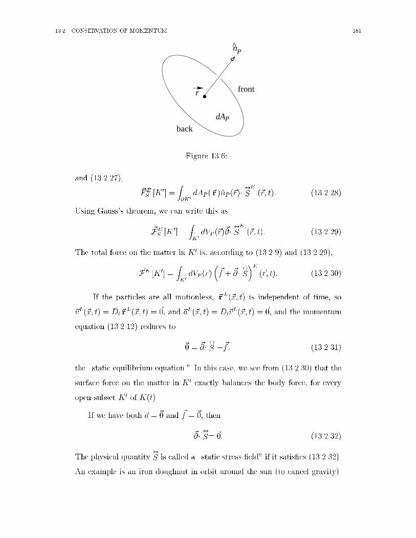
����� CONSERVATION OF MOMENTUM ���
.back
front
^
r
dA
nP
P
Figure ����
and �������
�FES �K �� �
Z�K�
dAP ��r � nP ��r���
SE��r� t�� ������
Using Gauss�s theorem� we can write this as
�FES �K �� �
ZK�
dVP ��r����
SE��r� t�� ������
The total force on the matter in K � is� according to ������ and �������
�FE �K �� �ZK�
dVP ��r���f � �� �S
�E��r� t�� ������
If the particles are all motionless� �r L��x� t� is independent of time� so
�vL��x� t� � Dt�rL��x� t� � ��� and �aL��x� t� � Dt�v
L��x� t� � ��� and the momentum
equation ������ reduces to
�� � �� �S ��f� ������
the �static equilibrium equation�� In this case� we see from ������ that the
surface force on the matter in K � exactly balances the body force� for every
open subset K � of K�t��
If we have both �a � �� and �f � ��� then
�� �S� ��� �����
The physical quantity�
S is called a �static stress �eld� if it satis�es ������
An example is an iron doughnut in orbit around the sun �to cancel gravity��
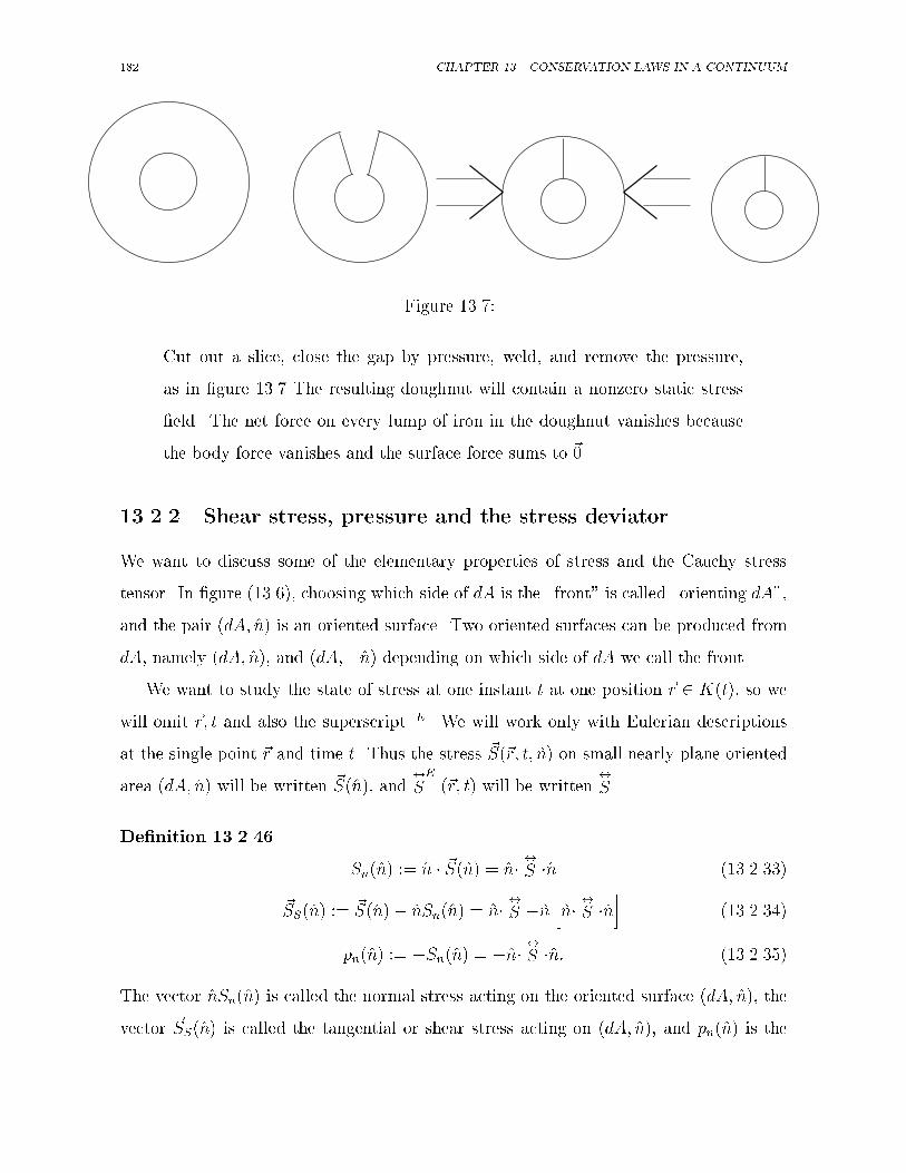
��� CHAPTER ��� CONSERVATION LAWS IN A CONTINUUM
Figure ����
Cut out a slice� close the gap by pressure� weld� and remove the pressure�
as in �gure ��� The resulting doughnut will contain a nonzero static stress
�eld� The net force on every lump of iron in the doughnut vanishes because
the body force vanishes and the surface force sums to ���
������ Shear stress� pressure and the stress deviator
We want to discuss some of the elementary properties of stress and the Cauchy stress
tensor� In �gure ������ choosing which side of dA is the �front� is called �orienting dA��
and the pair �dA� n� is an oriented surface� Two oriented surfaces can be produced from
dA� namely �dA� n�� and �dA�� n� depending on which side of dA we call the front�
We want to study the state of stress at one instant t at one position �r � K�t�� so we
will omit �r� t and also the superscript E� We will work only with Eulerian descriptions
at the single point �r and time t� Thus the stress �S��r� t� n� on small nearly plane oriented
area �dA� n� will be written �S� n�� and�
SE��r� t� will be written
�
S�
De�nition �������
Sn� n� �� n � �S� n� � n� �S � n �����
�SS� n� �� �S� n�� nSn� n� � n� �S � n� n� �S � n
�������
pn� n� �� �Sn� n� � � n��
S � n� ������
The vector nSn� n� is called the normal stress acting on the oriented surface �dA� n�� the
vector �SS� n� is called the tangential or shear stress acting on �dA� n�� and pn� n� is the

����� CONSERVATION OF MOMENTUM ���
pressure acting on �dA� n��
Corollary �������
n � �SS� n� � � ������
�S� n� � nSn� n� � �SS� n� � � npn� n� � �SS� n�� ������
The shear stress is always perpendicular to n� parallel to dA� The normal stress acts
oppositely to n if pn� n� � ��
To visualize �S as a function of n� note that the set NP of unit vectors n � P is precisely
B���� ��� the spherical surface of radius � centered on �� in P � Thus �S attaches to each n
on the unit sphere NP a vector �S� n� whose radial part is nSN� n� and whose tangential
part is �SS� n�� This suggests
De�nition ������ The average value of pn� n� for all n � NP is called the average or
mean pressure at �r� t� It is written hpni��r� t�� We do not write the ��r� t� in this chapter�
Thus
hpni � �
��
ZNP
dA� n�pn� n� ������
where dA� n� is the element of area on NP �
Remark ������� hpni � ��� tr�
S
Proof�
Let y�� y�� y� be an orthonormal basis for P � and take components relative to
this basis� Then
pn� n� � � n��
S � n � �niSijnj � �Sijninj�
By the symmetry of NP �ZNP
dA� n�ninj � � if i �� j and
ZNP
dA� n�n�� �ZNP
dA� n�n�� �ZNP
dA� n�n�� �ZNP
dA� n��n�� � n�� � n���
�
��
�

��� CHAPTER ��� CONSERVATION LAWS IN A CONTINUUM
Therefore� ZNP
dA� n�ninj ���
�ij and
hpni � � �
� �Sij
ZNP
dA� n�ninj � ��
�ijSij
� ��
Sii � ��
tr
�
S �
Only part of�
S produces the shear stress �SS� n�� To see this we need a brief discussion
of tensors in U � U � where U is any Euclidean space�
Lemma ������� tr�
I U� dimU �
Proof�
Let y�� � � � � yn be an orthonormal basis for U � Then�
I U� yi yi and tr�
I U�
yi � yi � n � dimU �
Lemma ������� If�
S� U � U � tr�
S��
I U hi�
S�
Proof�
With yi as above� tr�
S� Sii � �ijSij � ��
I U�ijSij ��
I U hi�
S�
De�nition �������
S� U � U is �traceless�� or a �deviator� if tr�
S� ��
Corollary ��������
S is a deviator� �
S is orthogronal to all isotropic tensors in U �U �
Proof�
The isotropic tensors are the scalar multiples of�
I U � But�
S is orthogonal to�
I U��
S hi �I U� �� Now use lemma ����
Remark ������� If�
S� U � U � there is exactly one isotropic tensor ��
I U and one
deviator�
SD such that�
S� ��
I U ��
SD � ������
����� CONSERVATION OF MOMENTUM ���
Proof�
Uniqueness� Since tr�
SD� �� ������ implies tr�
S� � tr�
I U� ��dimU��
Thus � is uniquely determined by�
S � Then� from ������� the same is true
of�
SD�
Existence� Choose � � �tr�
S�� dimU and de�ne�
SD by ������� Then
tr�
S� ��tr�
I U� � tr�
SD� tr�
S �tr�
SD so tr�
SD� ��
De�nition ������ In ������� ��
I U is the isotropic part of�
S� and�
SD is the deviatoric
part of�
S� If U � P and�
S is a Cauchy stress tensor��
SD is the stress deviator�
Remark ������� Suppose ��
I P and�
SD are the isotropic and deviatoric parts of Cauchy
stress tensor�
S� Then
i� hpni � �� �
ii� If�
S� ��
I P �i�e���
SD���� then pn� n� � �� for all n and
�
SS � n� � �� for all n�
iii��
S and�
SD produce the same shear stress for all n �i�e�� the shear stress is due entirely
to the deviatoric part of�
S��
Proof�
i� By ������ tr�
S� �� By remark �������� tr�
S� �hpni�
ii� Substitute ��
I P for�
S in ������ and �������
iii� From ������� if n is �xed� �SS� n� depends linearly on�
S� By �������
�SS� n� is the sum of a contribution from ��
I P and one from�
SD� By ii�
above� the contribution from ��
I P vanishes�
Remark ������� If a Cauchy stress tensor produces no shear stress for any n� it is
isotropic�
Proof�

��� CHAPTER ��� CONSERVATION LAWS IN A CONTINUUM
The hypothesis is� from ������� that n� �S� nSn� n� for all unit vectors n�
Let y�� y�� y� be an orthonormal basis for P � Then setting n � yi gives
yi��
S� yi�Sn� yi��� But�
S��
I P ��
S� � yi yi���
S� yi� yi��
S� �P
yi yiSn� yi��
That is�
S��Xi �
yi yiSn� yi��
But then�
ST��
S� so n� �S � yi � yi��
S � n� and thus nSn� n� � yi � yiSn� yi� � n� orSn� n�� n � yi� � Sn� yi�� n � yi�� This is true for any n� so we may choose an n
with n � yi �� � for all of i � �� � � Then Sn� n� � Sn� y�� � Sn� y�� � Sn� y���
so�
S� Sn� n� yi yi � Sn� n��
I P � QED
Fluid Motion�
As an application of Cauchy stress tensors and the momentum equation� we consider
certain elementary �uid problems�
De�nition ������� A �uid is a material which cannot support shear stresses when it
is in static equilibrium� A non�viscous �uid is a material which can never support shear
stresses�
Corollary ������ In a non�viscous �uid� or in a �uid in static equilibrium� the Cauchy
stress tensor is isotropic� and�
SE��r� t� � �hpni��r� t�
�
I P �
Proof�
From remark ���������
SE
��r� t� � ���r� t��
I P � From remark ����� i��
� � �hpni�
De�nition ������� In a non�viscous �uid� or in a �uid in static equilibrium� hpni iscalled simply �the� pressure� written p� Thus
�
S� �p �
I P � �������
Remark ������� � � �p �
I � � �p�
����� CONSERVATION OF MOMENTUM ��
Proof�
By exercise ��a� � � �p �
I P � � �p� �I P �p�� �I P � But �� �I P��
I P hi��
I P� �
because�
I P is constant and ��
I P� �� Also �p� �I P� �p� QED�
Therefore� the Eulerian momentum equation in a non�viscous �uid is
��a � ��p� �f� �������
Since �a � Dt�u � t�u� �u � ��u� this is often written
��t�u� �u � ��u
�� ��p� �f� ������
In a �uid in static equilibrium� ��a � ��� so
�p � �f� ������
Therefore� � � �f � ��� We have
Remark ������� Static equilibrium in a �uid subjected to body force �f is impossible
unless � � �f � ���
Remark ������ If a �uid is in static equilibrium in a gravitational �eld� then the pres�
sure and density of the �uid are constant on gravitational equipotential surfaces which
are arcwise connected�
Proof�
Let + be the gravitational potential� Then �f � ���+� so ������ shows
that �p is a scalar multiple of �+� And � � �f � ���� �+� Since � � �f � ���
�� is also a scalar multiple of �+� Therefore� if C is any curve lying in a
gravitational equipotential surface� and if � ��r� is the unit tangent vector to C
at �r� then �� ��r� � ����r� � ���r� � �p��r� � �� Therefore� by theorem ����� �
and p are the same at both ends of C�

��� CHAPTER ��� CONSERVATION LAWS IN A CONTINUUM
���� Lagrangian form of conservation of momentum
We use the notation introduced on page ��� If �x is a point in label space L� we use
dVL��x� to stand for a small set containing �x and also for the volume of that set� The
mass per unit volume in label space is �L��x�� independent of time� so the total mass of the
particles whose labels are in dVL��x� is �L��x�dVL��x�� Their velocity at time t is �vL��x� t��
so their momentum is dVL��x� �L��x��vL��x� t�� The total momentum of the particles whose
labels are in open subset H � of H is� at time t�
�PLt �H �� �
ZH�
dVL��x� �L��x��vL��x� t� �
ZH�
dVL��x�� ��v�L��x� t��
Let �FLt �H
�� denote the total force exerted on those particles at time t� Then the law of
conservation of momentum requires
d
dt�PLt �H �� � �FL
t �H �� � ������
Since the set H � does not vary with time� we also have the mathematical identity
d
dt�PLt �H �� �
ZH�
dVL��x� �L��x�Dt�v
L��x� t��
ord
dt�PLt �H �� �
ZH�
dVL ��x� � ��a�L ��x� t� � �����
The particles whose labels are in H � occupy the set K ��t� in physical space P at time
t� Therefore �PLt �H
�� � �PE�K ��t��� and ����� should agree with ������ That it does
can be seen by changing the variables of integration from �r to �x in ����� by means of
�������� and then using �������
Let �FLB�t�H
�� denote the total body force on the particle with labels in H �� Then
�FLB�t�H
�� � �FEB �K
��t��� By changing the variables of integration in ������ from �r to �x
via ��������� we �nd
�FLB�t �H
�� �ZH�
dVL��x����det �D�r L��x� t�
��� �fL��x� t��or
�FLB�t �H
�� �ZH�
dVL��x�� fL
��x� t� �����

����� LAGRANGIAN FORM OF CONSERVATION OF MOMENTUM ���
.back
front
^
( )
x
dAL x
nL
Figure ����
where
� f ����det �D�r
��� �f� ������
The vector � f is the body force density per unit of label�space volume� Formula ������
can be seen physically as follows� The body force on the particles in the small set dVP ��r�
is dVP ��r��fE��r� t� at time t� But these are the particles whose labels are in dVL��x�� so by
������� this force is dVL��x�� fL
��x� t� with � f given by �������
The surface force at time t exerted by the particles whose labels are just outside H �
on the particles whose labels are just inside H � we will denote by �FLS�t�H
��� The particles
with labels just outside �inside� H � are those whose positions at time t are just outside
�inside� K ��t�� so
�FLS�t �H
�� � �FES �K ��t�� � ������
Then �FLt �H �� � �FL
B�t �H�� � �FL
S�t �H��� It remains to study the surface force �FL
S�t�H���
Let dAL��x� be any small nearly plane patch of surface in label space L containing the
label �x � H� Choose one side of dAL to be the front� and let nL be the unit normal to
dAL��x� on its front side� Figure ��� is the same as �gure ����� except for the labelling�
Now� however� the picture is of a small patch of surface in label space� not physical space�
The force d �FS exerted by the particles with labels just in front of dAL on the particles
with labels just behind dAL is proportional to dAL� as long as the orientation of that small
surface does not change� i�e�� as long as nL is �xed� We denote the vector �constant� of
proportionality by � S� Then d �FLS � � SdAL� The vector � S will change if nL changes� and it

��� CHAPTER ��� CONSERVATION LAWS IN A CONTINUUM
^ ( )
x
L xn
H H
.
∂ ′ ′
Figure ����
also will depend on �x and t� so at time t at label �x
d �FLS � � S��x� t� nL�dAL��x�� ������
�Compare ������� The vector � S we call the �label stress�� The total surface force on
the particles in H � is then
�FLS�t �H
�� �Z�H�
dAL��x�� S ��x� t� nL��x�� ������
where nL��x� is the unit outward normal to H � at �x � H �� Now we can combine �����
and ������ to obtain
�FLt �H �� �
ZH�
dVL��x� fL��x� t� �
Z�H�
dAL��x�� S ��x� t� nL��x�� � ������
Inserting this and ����� in ������ givesZH�
dVL��x�� ��a� � f
�L��x� t� �
Z�H�
dAL��x�� S ��x� t� nL��x�� � ������
Equation ������ is true for every open subset H � ofH for which H � is piecewise smooth�
It is mathematically of the same form as ������� and the same application of Cauchy�s
theorem ������ shows that there is a unique tensor� SL
��x� t� � L�P such that for every
unit vector nL � L�
� S��x� t� nL� � nL��
SL��x� t�� �������
The tensor� SL
��x� t� is the Piola�Kircho� or body stress tensor� We would prefer to call
it the label stress tensor� but history prevents us� Proceeding in the way which led from

����� LAGRANGIAN FORM OF CONSERVATION OF MOMENTUM ���
������� to ������ we note that by Gauss�s theoremZ�H�
dAL��x� nL��
SL��x� t� �
ZH�
dVL��x� �D��
SL��x� t�
so ZH�
dVL��x�
� ��a� � f � �D �
� S
�L
��x� t� � ��
Since this is true for all open H � � H with H � piecewise smooth� the vanishing integral
theorem gives
��a � � f � �D �� S� �������
This is the Lagrangian form of the momentum equation� Equation ������ can now be
written
d �FLS � dAL��x� nL �
� SL
��x� t�� ������
where d �FLS � dAL��x� and nL refer to �gure ����
Equations ������� and ������ refer to the same motion� The relation between �
and � is ������� The relation between � f and �f is ������� which can also be written
� f
��
�f
�� ������
both sides of this equation being the force per unit mass on the material� But what is the
relation between� S and
�
S$
Suppose that dAL��x� is a small nearly plane surface in label space L� and that we
have chosen one of its sides as the front� Let nL be the unit normal to dAL��x� on its
front side� At time t� let �r � �r L��x� t�� Let dAP ��r� be the small nearly plane surface
in physical space P consisting of all positions at time t of particles whose labels are in
dAL��x�� Let dAL��x� and dAP ��r� denote both the sets of points which make up the small
surfaces and also the areas of those sets� Choose the front side of dAP ��r� so that particles
are just in front of dAP ��r� if their labels are just in front of dAL��x�� Let nP be the unit
normal to dAP ��r� on its front side� Then the force exerted on the particles just behind
dAP ��r� by the particles just in front can be written either as dAP ��r� nP ��
SE��r� t� or as
dAL��x� nL �� SL
��x� t�� Therefore� these two expressions must be equal�
dAP ��r� nP ��
SE��r� t� � dAL��x� nL �
� SL
��x� t� �������

��� CHAPTER ��� CONSERVATION LAWS IN A CONTINUUM
.front
backback
front
^
( )
^
( )
n
dA
L
L x
nP
rdA rP
.x
Figure �����
if
�r � �r L��x� t� �������
and
dAP ��r� �h�r L��� t�
i�dAL��x�� � �������
Notice that in �������� dAP and dAL are positive real numbers� areas� while in �������
they stand for sets� the small surfaces whose areas appear in ��������
Our program is to express dAP ��r� nP in terms of dAL� x� nL in �������� to cancel
dAL� x� nL� and thus to obtain the relation between�
S and� S� Equation ����� holds�
whatever the shape of dAL��x�� It is convenient to take it to be a small parallelogram
whose vertices are �x� �x � ���� �x � ���� �x � ��� � ���� Then dAP ��r� will be a very slightly
distorted parallelogram with vertices
�r � �r L��x� t�
�r � ��� � �r L��x� ���� t�
�r � ��� � �r L��x� ���� t�
�r � ��� � ��� � �r L��x� ��� � ���� t��
Correct to �rst order in the small length k��ik� we have
�r � ��i � �r L��x� t� � ��i � �D�r L��x� t��
so
��i � ��i � �D�r L��x� t�� �������

����� LAGRANGIAN FORM OF CONSERVATION OF MOMENTUM ���
nP
.front
back
ξ
+ ξ+ ξ + ξ
( )
ξ + ξ+ ρ
ρ
+ ρ
( )
+ ρ + ρ
2
x2
x
1 x1
dA xL
x1 2
1
nL
r r2
dA rP
r11 2r
. .
.
Figure �����
We naturally take ��� and ��� in di�erent directions� so k�������k �� � �recall that L and P are
oriented �spaces� so cross products are de�ned�� We number ��� and ��� in the order which
ensures that ��� � ��� points into the region in front of dAL��x�� so ��� � ��� � k��� � ���k nL�But k��� � ���k � dAL��x�� so
dAL��x� nL � ��� � ���� �������
Also� clearly� k�������k � dAP ��r�� and ������� is perpendicular to dAP ��r�� so ������� ��k��� � ���k nP � Thus
dAP ��r� nP � ���� � ���� �������
But which sign is correct$ We have to work out which is the front side of dAP ��r�� because
that is where we put nP � If ��� � L is small� �x � ��� is in front of dAL��x� � ��� � nL � ��
and hence ���� �
���� � ���
�� �� ������
The particle with label �x� ��� has position �r � ���� with ��� given by �������� Then���������������������������
��� � ���� � ���� � AP ����� ���� ���� � AP ����� ���� ����
� AP
���� � �D�r L� ��� � �D�r L� ��� � �D�r L
�
�hdet �D�r L��x� t�
iAL
����� ���� ���
��hdet �D�r L��x� t�
i��� �
���� � ���
��
������

��� CHAPTER ��� CONSERVATION LAWS IN A CONTINUUM
Thus the position �r � ��� is in front of dAP ��r� � ��� � ���� � ���� has the same sign as
det �D�r L��x� t�� Let sgn c stand for the sign of the real number c� That is� sgn c � �� if
c � �� � �� if c �� and � � if c � �� Then position �r � ��� is in front of dAP ��r��
sgn ��� � ���� � ���� � sgn det �D�r L��x� t�� �����
We have chosen the front of dAP ��r�� and the direction of nP � so that �r � � nP is in front
of dAP ��r� when � � �� Therefore sgn nP � ���� � ���� � sgn det �D�r L��x� t�� Thus
��� � ��� � k��� � ���k nP sgn det �D�r L��x� t�
and
dAP ��r� nP � ���� ���� sgn det �D�r L��x� t�� �����
Using ������� and ������ we hope to relate to dAP nP and dAL nL� so we try to
relate ��� � ��� and ��� � ���� The two ends of ������ give
��� � ���� � ���� � ��� ����� � ���
�det �D�r L��x� t� ������
for any ���� ���� ��� � L� if ���� ���� ��� are given by ��������
Substituting ������� and ����� in ������ and using c sgn c � jcj� we �nd
��� � �dAP ��r� nP � � ��� � �dAL��x� nL����det �D�r L��x� t�
��� �But ��� � ��� � �D�r L��x� t�� so
��� � �D�r L��x� t� � �dAP ��r� nP � � ��� � �dAL��x� nL����det �D�r L��x� t�
��� �Since this is true for any ��� � L� we must have
�D�r ���x� t� � �dAP ��r� nP � � dAL��x� nL���det �D�r L��x� t�
���or� letting T stand for transpose�
dAP ��r� nP �h�D�r L��x� t�
iT� dAL��x� nL
���det �D�r L��x� t���� � ������

����� LAGRANGIAN FORM OF CONSERVATION OF MOMENTUM ���
If we dot� SL
��x� t� on the right of each side of ������� we obtain
dAP ��r� nP � �D�r L��x� t�T �� SL
��x� t�
� dAL��x� nL �� SL
��x� t����det �D�r L��x� t�
��� � ������
But �see ������
d �FS � dAL��x� nL �� SL
��x� t� � dAP ��r� nP ��
SE��r� t�
where �r � �r L��x� t�� Thus
dAL��x� nL �� SL
��x� t� � dAP ��r� nP ��
SL��x� t��
Substituting this on the right side of ������ gives
�dAP ��r� nP � ���D�r L��x� t�T �
� SL
��x� t�
�
� �dAP ��r� nP � ���
SL��x� t�
���det �D�r L��x� t����� � ������
We have proved ������ when dAP is a small parallelogram� as in Figure �������� But
��� and ��� can be arbitrary as long as they are small� Hence so can dAP ��r� nP � ��� � ����
Thus ������ is true when dAP ��r� nP is any small vector in P � Since ������ is linear
in dAP ��r� nP � it is true whatever the size of that vector� Therefore ������ implies
�D�r L��x� t�T �� SL
��x� t� ��
SL��x� t�
���det �D�r L��x� t���� �
or ��D�r
�T � � S ��
S���det �D�r
��� � ������
This gives�
S in terms of� S� By ������ ������ �D�r L��x� t� has an inverse� � �x E��r� t��
where �r � �r L��x� t�� so �D�r L��x� t�T has the inverse � �x E��r� t�T � Dotting this on the left
in ������ gives� S �
�� �x
�T � �S ���det � �x ����� ������
where we use det� �D�r ��� � �det �D�r����

��� CHAPTER ��� CONSERVATION LAWS IN A CONTINUUM
By appealing to ������� we can write ������ and ������ as���
S
�
A ���D�r
�T ��B�� S
�
CA ������
�B�� S
�
CA ��� �x
�T ����
S
�
A � ������
��� Conservation of angular momentum
����� Eulerian version
Refer again to the notation on page ��� All torques and angular momenta are calculated
relative to the origin �OP in physical space P � Let �LE�K ��t�� denote the total angular
momentum of the particles in K ��t�� while �ME�K ��t�� denotes the total torque on them�
The law of conservation of angular momentum is
d
dt�LE �K ��t�� � �ME �K ��t�� � �������
Our problem is to express this law locally�
The momentum of the particles in dVP ��r� is dVP ��r��E��r� t��vE��r� t� and this produces�
relative to �OP � the angular momentum
�r �hdVP ��r����v�
E��r� t�i� dVP ��r���r � ��v�E��r� t��
It is possible that the individual atoms in dVP ��r� might have angular momentum� this
might be from the orbits of electrons not in closed shells� from the spins of unpaired elec�
trons� or from nuclear spin� Orbital angular momentum is quantized in integer multiples
of 'h� while spin angular momentum is in units of 'h�� Here 'h � h�� and h is Planck�s
constant� so 'h � ������ � ���� joule sec� If the atoms are not randomly aligned� there
may be an intrinsic atomic angular momentum of �lE��r� t� per kilogram at position �r at
time t� Then the intrinsic angular momentum in dVP ��r� is dVP ��r����l�E��r� t�� and the total
angular momentum in dVP ��r� is
d �LE � dVP ��r�h���r � �v ��l
�iE��r� t��

����� CONSERVATION OF ANGULAR MOMENTUM ��
Figure ����
The total angular momentum in K ��t� is
LE �K ��t�� �ZK�t�
dVP ��r�h���r � �v ��l
�iE��r� t��
From ��������
d
dtLE �K ��t�� �
ZK�t�
dVP ��r�h�Dt
��r � �v ��l
�iE��r� t��
Now
Dt��r � �v� � �Dt�r�� �v � �r �Dt�v � �v � �v � �r � �a � �r � �a�
sod
dtLE �K ��t�� �
ZK�t�
dVP ��r�h���r � �a �Dt
�l�iE
��r� t�� ������
To calculate the torque on the particles in K ��t� we note that the torque exerted by the
body force dVP ��r��fE��r� t� is �r�dVP ��r��fE��r� t�� or dVP ��r���r� �f �E��r� t�� The torque exerted
by the surface force dAP ��r��S��r� t� nP � is �r�dAP ��r��S � �dAP ��r��S��r � �dAP ��r�� n��
SE
��r� t�� � �r� If�
Q� P � P is a polyad� � n� �Q� � �r � n � ��Q ��r�� so this is true for all�
Q�
�Exercise ��b gives a de�nition of �r� �
Q� and�
Q ��r is de�ned similarly�� Thus
�r � dAP ��r��S��r� t� nP � � �dAP ��r� nP ���
S ��r�E
��r� t��

��� CHAPTER ��� CONSERVATION LAWS IN A CONTINUUM
.back
front^
( )
r
n
dA rP
P
Figure ����
Therefore� the torque about �OP which is exerted on the particles in K ��t� by the body
and surface force acting on them is
ZK�t�
dVP ��r��vecr � �f
�E��r� t��
Z�K�t�
dAP ��r� nP ���
S ��r�E
��r� t��
By applying Gauss�s theorem to the surface integral� we can write this torque as
ZK�t�
dVP ��r���r � �f � � �
��
S ��r��E
��r� t�� ������
In addition to this torque� there may be a torque acting on each atom in dVP ��r��
This would be true� for example� if the material were a solid bar of magnetized iron
placed in a magnetic �eld �B� If the magnetization density was �M � there would be a
torque dVP ��r� �M � �B acting on dVP ��r� and not included in ������� In general� we might
want to allow for an intrinsic body torque of �m joules�meter�� so that ������ must be
supplemented by a term ZK�t�
dVP ��r��mE��r� t��
Finally� in a magnetized iron bar� atoms just outside K ��t� exert a torque on atoms
just inside K ��t�� so there is a �torque stress� acting on K ��t�� The torque exerted on
the material just behind dAP ��r� by the material just in front is proportional to dAP as
long as the orientation of that small patch of surface� i�e�� its unit normal� stays �xed�
We write the proportionality constant as �M��r� t� nP �� The torque exerted on the material
just behind dAP by the material just in front� other than that due to nP ��
SE
��r� t�� is

����� CONSERVATION OF ANGULAR MOMENTUM ���
�M��r� t� nP �dAP ��r�� so we must also supplement ������ by a term
Z�K�t�
dAP ��r� �M ��r� t� nP ��r� t�� �
where nP is the outward unit normal to K ��t�� Thus we �nally have
�ME �K ��t�� �ZK�t�
dVP ��r���r � �f � � �
��
S ��r�� �m
�E��r� t�
�Z�K�t�
dAP ��r� �M ��r� t� nP ��r� t�� � �������
If we substitute ������ and ������� in �������� we obtain
RK�t� dVP ��r�
����r � �a�Dt
�l�� �r � �f � � �
��
S ��r�� �m
�E��r� t�
�R�K�t� dAP ��r� �M ��r� t� nP ��r� t�� � �������
This equation has the same mathematical form as �������� and leads via Cauchy�s the�
orem to the same conclusion� At �r� t there is a unique tensor�
ME ��r� t� � P � P � which
we call the �Cauchy� torque�stress tensor� such that for every unit vector nP � P we have
�M ��r� t� nP � � nP ��
ME ��r� t� �� �������
Substituting this on the right in �������� applying Gauss�s theorem to the surface integral�
and the vanishing integral theorem to the volume integral� gives
���r � �a �Dt
�l�� �r � �f � � �
��
S ��r�� �m � � � �M� �������
Before we accept this as the Eulerian angular momentum equation� we note that it can be
greatly simpli�ed by using the momentum equation ������� We have ���r � �a� � �r � �f
� �r ����a� �f
�� �r � ��� �S�� so ������� is
�Dt�l � �r �
��� �S
�� � �
��
S ��r�� �m� �� �M � �������
This can be still further simpli�ed� Let y� � y�� y� be a poob in P � � x�� x�� x�� a pooob in
L� and take components relative to these bases� Then
��r � ��� �S�
�i� �ijkrj���
�
S�k � �ijkrjlSlk�

��� CHAPTER ��� CONSERVATION LAWS IN A CONTINUUM
Also� for �u � �v� �w � P � ��u�v�� �w � �u��v� �w� �this is how we use the lifting theorem to
de�ne�
Q ��w for�
Q� P � P and �w � P � so
���u�v�� �w�ij � ��u ��v � �w��ij � ui ��v � �w�j
� ui�jkl�kwl
� ��u�v�ik �jklw�
Therefore for any�
Q� P � P �
��
Q ��w�ij� Qik�jklwl�
Therefore
��
S ��r�li
� Slk�ikjrj�� �
��
S ��r��
i� l
��
S ��r�li� l �Slk�ikjrj�
� �ikjl �Slkrj�
� �ikj ��lSlk� rj � Slklrj� �
Referring to page ��� and using �ijk � �ijk � �� we get
��r �
�� � �S
�� � �
��
S ��r��
i� �ikjSlklrj�
But lrj � �lj� so this is �ikjSjk � ��ijkSjk � ��AP hi
�
S
�i� Thus
�r ���� �S
�� � �
��
S ��r�� �AP hi
�
S � �������
Thus ������� is
�Dt�l � AP hi
�
S ��m� �� �M � ��������
This is the Eulerian form of the angular momentum equation� In non�magnetic materials
it is believed that �l� �m are�
M and all negligible� and that the essential content of ��������
is
AP hi�
S� ��� ��������

����� CONSERVATION OF ANGULAR MOMENTUM ���
That is� �ijkSjk � �� Multiply by �ilm and sum on i� and this becomes �see page D���
��jl�km � �jm�kl�Sjk � ��
or
Slm � Sml � ��
or�
ST��
S � �������
The conservation of angular momentum requires that the Cauchy stress tensor be sym�
metric� if intrinsic angular momentum� body torque and torque stress are all negligible�
����� Consequences of�
ST�
�
S
In the absence of intrinsic angular momentum� torque and torque stress� the Cauchy stress
tensor is symmetric� This greatly simpli�es visualizing the stress at a point �r at time t�
We will abbreviate�
SE��r� t� as
�
S in this chapter� because we are looking at one time t and
one position �r in physical space� We denote by �S� n� the stress on the oriented small area
�dA� n� at �r� t �i�e� we write �S��r� t� nP � as �S� n�� and nP as n� dAP as dA�� We denote by
S the linear operator on P corresponding to the tensor�
S� Then for any unit vector n�
�S� n� � n� �S� S� n�� �������
Since S � P P is a symmetric operator� P has an orthonormal basis x� y� z consisting
of eigenvectors of S� That is� there are scalars a� b� c such that
S� x� � a x� S� y� � b y� S� z� � c z� ��������
Then x� �S� a x� y� �S� b y� z� �S� c z so
�
S��
I P ��
S� � x x� y y � z z� � �S� x �a x� � y �b y� � z �c z�
so�
S� a x x � b y y � c z z� ��������
��� CHAPTER ��� CONSERVATION LAWS IN A CONTINUUM
The unit vectors x� y� z are called �principal axes of stress� and a� b� c are �principal
stresses�� By relabelling� if necessary� we can always assume that a � b � c� Also if we
change the sign of any of x� y� z both �������� and �������� remain unchanged� Therefore
we may assume that � x� y� z� is positively oriented�
For any vector �n � P we write
�n � x x � y y � z z� ��������
The unit sphere NP consists of those �n � P for which
x� � y� � z� � �� ��������
The pressure pn� n� acting on �dA� n� is pn� n� � � n��
S � n � ��ax�� by�� cz��� It can be
thought of as a function of position n � x x � y y � z z on the spherical surface ���������
In the earth� pn � �� so it is convenient to introduce the principal pressures A� B� C�
de�ned by
A � �a� B � �b� C � �c� ��������
Then A � B � C� The cases where equality occurs are special and are left to the reader�
We will examine the usual case�
A B C� ��������
We want to try to visualize pn� n� and the shear stress �SS� n� acting on �dA� n� as func�
tioning of n� i�e�� as functions on the spherical surface ���������
We have
pn� n� � Ax� �By� � Cz� �������
�S� n� � �SS� n�� pn� n� n �������
and� since �S� n� � n� �S��S� n� � �Ax x� By y � Cz z� ������
First consider pn� Its value is unchanged if we replace any of x� y� z by its negative
in ��������� Therefore pn is symmetric under re�ections in the coordinate planes x � ��
����� CONSERVATION OF ANGULAR MOMENTUM ���
y � �� z � �� Therefore it su!ces to study pn� n� when n is in the �rst octant of ���������
i�e�� when
x � �� y � �� z � �� ������
If p is any constant� then the level line pn� n� � p on Np satis�es
Ax� �By� � Cz� � p �������
x� � y� � z� � �� �������
Hence� it satis�es
�A� p� x� � �B � p� y� � �C � p� z� � �� �������
This equation and �������� have no real solutions �x� y� z� unless
A � p � C� �������
so the values of pn� n� all lie in the interval �������� The value p � A requires y � z � ��
x � ��� so pn� n� � A only for n � � x� The value p � C requires x � y � �� so pn� n� � C
only for n � � z� The value of p � B makes ������� into xpB � A � �zpC � B�
and these two planes intersect the sphere �������� in great circles� one of which lies in
������� For any value of p in A p C� ������� and ������� imply all three of the
following� ��������������C � A�x� � �C �B� y� � C � p
�B � A� x� � �C � B� z� � B � p
�B � A� y� � �C � A� z� � p� A�
�������
Therefore the projection of the level curve �������� �������� onto the xy or yz plane is
part or all of an ellipse� and its projection on the xz plane is part of a hyperbola with
asymptotes xpB � A � �zpC � B� The level lines pn� n� � B on Np� with p � B�
are the great circles where Np intersects the planes xpB � A � �zpC � B� The level
lines of pn on NP are the dashed curves in �gure ����� Next� consider the shear stress
�SS� n�� At any n � NP � this is a vector tangent to NP � It is de�ned by �������� and
from ������ �S� n� � ��� �pn� n� where pn is to be considered as a function de�ned
for all �n � P by �������� even when k�nk �� �� At a point n � NP � let �� n� be the unit

��� CHAPTER ��� CONSERVATION LAWS IN A CONTINUUM
np = C
p = Bn
p = An
p = Bn
^
^
^
z
x
y
Figure �����

����� CONSERVATION OF ANGULAR MOMENTUM ���
vector tangent to the level curve of pn passing through n� Then n � � � n� � �� and since
�� n� is tangent to a curve lying in the level surface pn��n� � constant in P � it follows that
�� n� � �pn� n� � �� Therefore� from �������� we have
� � n� � �S� n� � �
and
�� n� � n � ��
Then from �������� � � n� � �SS� n� � �� Thus the shear stress �SS� n� at n � NP is
perpendicular to the level line of pn which passes through n� The �lines of force� of the
shear stress on NP are the curves which are everywhere tangent to �SS� n�� They are the
solid curves in �gure ����� and are everywhere perpendicular to the level lines of pn�
These �lines of force� give the direction of �SS� n� everywhere on NP �
Finally� we would like to �nd k�SS� n�k on NP � which we abbreviate as
�� n� � k�SS� n�k� �������
Again we consider only the �rst octant� x � �� y � �� z � �� The other octants are
obtained by re�ection in the three coordinate planes x � �� y � �� z � �� First consider
the edges of the �rst octant� where x � � or y � � or z � �� On the quarter circle
n � x cos � � y sin �� � � � � ��� subjecting ������� and �������� ������ to a little
algebra yields
�SS� n� � sin � cos � � x cos � � y sin �� on n � x cos � � y sin �� �������
Therefore� from ��������
�� n� ��
�B � A� sin � if n � x cos � � y sin �� �������
This reaches a maximum value of �B � A�� at � � ���� half way between x and y on
the quarter circle� And �� x� � �� y� � �� Similarly
�� n� � ���C � A� sin � if n � x cos � � z sin � ������
�� n� � ���C � B� sin � if n � y cos � � z sin �� ������
To see what happens to �� n� when x � �� y � �� z � �� we appeal to

��� CHAPTER ��� CONSERVATION LAWS IN A CONTINUUM
Lemma ������� On any level line of pn in the �rst octant on NP � �� n� decreases mono�
tonically as y increases�
Proof�
From �������� k�S� n�k� � �� n�� � pn� n�� so
�� n�� � k�S� n�k� � pn� n��� �������
We can parametrize the level curve pn� n� � p on NP by the value of y at n�
namely y � n � y� We want to show that
d
dy�� n� � on the curve pn� n� � p on NP
�s �rst octant� �������
On that level curve� of course pn� n� is constant� so ������� shows that
������� is equivalent to
d
dyk�S� n�k� � on the curve pn� n� � p on Np
�s �rst octant� �������
The vector d n�dy on pn� n� � p is tangent to that level curve� Hence n �d n�dy � � and �p� n� � d n�dy � �� so �S� n� � d n�dy � �� Hence� for some
d n
dy� n� �S� n��
Now d n�dy � x�dx�dy� � y � z�dz�dy� on the level curve� Hence
y � d ndy
� �� so � � y � n� �S� n��
But n � xx � yy � zz� ��S� n�Ax x �By y � Cz z� so
� y � n� �S� n� �
������������ � �
x y z
Ax By Cz
������������ �xz�C � A��
Thus � ��xz�C � A�� and
d n
dy�
�
xz�C � A� n� �S� n�� �������

����� CONSERVATION OF ANGULAR MOMENTUM ��
By the chain rule� ddyk�S� n�k� � d�n
dy� �k�S� n�k�� From �������
k�S��n�k� � A�x� �B�y� � C�z�� so
�k�S��n�k� � A�x x � B�y y � C�z z�
Therefore
d
dyk�S� n�k� �
xz�C � A�
h n� �S� n�
i��A�x x �B�y y � C�z z
�
�
xz�C � A�
�����������x y z
�Ax �By �CzA�x B�y C�z
������������ � y
�C � A�
������������ � �
A B C
A� B� C�
������������ �y�C � B��B � A� ��
This proves lemma ����� �
QED�
From ������� ����� ����� and lemma ����� we infer that the largest value of
�� n�� the magnitude of the shear stress� is �C�A��� and this occurs at n � �� x� z��p�
and for no other n�
It is of some interest to see which pairs �pn� n�� �� n�� are possible on NP � On the three
quarter�circles in ������� ����� ����� we have�B� pn� n�
�n� n�
CA �
�B� A�B�� B�A
�cos �
B�A�
sin �
CA if n � x cos � � y sin � �z � �� �������
�B� pn� n�
�n� n�
CA �
�B� A�C�� C�A
�cos �
C�A�
sin �
CA if n � x cos � � z sin � �y � �� �������
�B� pn� n�
�n� n�
CA �
�B� B�C�� C�B
�cos �
C�B�
sin �
CA if n � y cos � � z sin �� �x � �� ��������
For z � �� the possible pairs �pn� n�� �� n�� are given by ������� and trace out the
seimicircle marked z � � in Figure ����� For y � �� the possible pairs are given by

��� CHAPTER ��� CONSERVATION LAWS IN A CONTINUUM
increases in the direction of the arrows.θ
MOHR
MOHR
.
.start
stop
A B C^
σ( )^
y = 0
z = 0
x = 0
n
n np ( )p
Figure �����

����� CONSERVATION OF ANGULAR MOMENTUM ���
������� and trace out the semicircle marked y � � in Figure ����� For x � �� use the
third semicircle in Figure ������
In �gure ����� suppose we start at a point with y � � and move along the level line
of pn till we hit either x � � or z � �� Then in the ��� pn� plane we will start at the point
marked �start� in Figure ����� and we will remain on the vertical dashed line pn � p�
According to lemma ����� as we increase y on the level curve pn� p in Figure �������
we will decrease �� n�� so we move down the dashed line in Figure ���� until we strike
the point marked �stop�� Therefore� the possible pairs �pn� n�� �� n�� which can occur on
NP are precisely the points in the shaded region in Figure �����
Coulomb suggested that a rock will break when the maximum value of �� n� exceeds
a critical value characteristic of that rock� Navier pointed out that when two plates are
pressed together� the greater this pressure the harder it is to slide one over the other�
Navier suggested that the fracture criterion is that there be an orientation n for which
�� n� � �c��pn� n�� where �c and � are constants characteristic of the rock �when p� n� � ��
Navier�s fracture criterion reduces to Coulomb�s�� The constant � is a sort of internal
coe!cient of friction� Mohr suggested that Coulomb and Navier had over�simpli�ed the
problem� and that the true fracture criterion is ��n� � f �p� n��� where f is a function
characteristic of the rock� which must be measured empirically� and about which one can
say in advance only that
f�p� � �� df�dp � �� ��������
Even with such a general criterion� much can be said� The curve � � f�p� is marked
�MOHR� in Figure ����� If A� B� C are moved so as to produce an overlap of the
shaded region with the Mohr curve� the rock will break at �rst contact of the curve and
the shaded region� This �rst contact will always occur on the plane y � �� at a value of
� in ���� which is between � and ���� so the normal to the plane of fracture will lie in
the xz plane� closer to x than to z� The circles in Figure ���� are called Mohr circles�

��� CHAPTER ��� CONSERVATION LAWS IN A CONTINUUM
��� Lagrangian Form of Angular Momentum
Conservation
Refer again to the notation introduced on page ��� If �LLt �H �� is the angular momentum
of the collection of particles with labels in H �� and �MLt �H
�� is the total torque on them�
the law of conservation of angular momentum is
d
dt�LLt �H �� �ML
t �H��� �������
Using the notation introduced on page ��� and page ����
�LLt �H �� �ZH�
dVL��x�h ��l � ��r � �v
iL��x� t�
sod
dt�LLt �H �� �
ZH�
dVL��x�h ��Dt�l � �r � �a
�iL��x� t� � ������
Moreover�
MLt �H
�� �ZH�
dVL ��x���r � � f � �m
�L��x� t�
�ZH�
dAL ��x�
��r �
� nL �
� SL�
� � M ��x� t� nL ��x��
�
where nL��x� is the unit outward normal to H � at �x � H �� � m is body torque per unit
of volume in label space� and � M��x� t� nL��x��dAL is the force exerted by the material with
labels just in front of �dAL� nL� on the material with labels just behind �dAL� nL�� Again
we have �r � � nL �� S� � �� nL �
� S�� �r � � nL � �
� S � �r�� so using Gauss�s theorem�
MLt �H
�� �ZH�
dVL ��x�
��r � � f � � m� �D �
�� S � �r
��L��x� t� ������
�ZH�
dAL ��x�� M ��x� t� nL��x�� � �������
Therefore
RH� dVL ��x�
� ��Dt�l � �r � �a
�� �r � � f � � m � �D �
�� S � �r
��
�R�H� dAL ��x�
� M ��x� t� nL��x�� � �������

����� CONSERVATION OF ENERGY ���
Applying Cauchy�s theorem to ������� shows that for each ��x� t� there is a unique� ML��x� t� � L� P such that for any unit vector n � L�
� M ��x� t� n� � n �
� ML
��x� t� � �������
If we substitute this on the right in ������� and use Gauss�s theorem and the vanishing
integral theorem� we obtain
�Dt�l � ��r � �a� �r � � f � � m � �D �
�� S � �r
�� �D �
� M�
Using the Lagrangian momentum equation �������� we can write this as
�Dt�l � �r �
��D �
� S
�� �D �
�� S � �r
�� �D �
� M � m�
Finally� by the sort of argument which led to �������� we can show
�r ���D �
� S
�� �D �
�� S � �r
�� �AP hi
���D�r�T � � S� �
so the Lagrangian form of the angular momentum equation is
�Dt�l � �D �
� M �
� m � AP hi
���D�r�T � � S� � �������
The relation between� M and
� M is the same as that between
� S and
�
S � If the intrinsic
angular momentum �l� body torque m� and torque stress� M are all negligible� �������
reduces to
AP hi���D�r�T � � S� � �� �������
A glance at ������ shows that ������� is the same as ��������� so we learn nothing
new from ������� in this case�
���� Conservation of Energy
����� Eulerian form
The velocity �vE��r� t� imparts to the matter in dVP ��r� a kinetic energy dVP ��r��E��r� t��
�k
�vE��r� t�k�� In addition� that material has kinetic energy of molecular motion� and the

��� CHAPTER ��� CONSERVATION LAWS IN A CONTINUUM
potential energy of the intermolecular forces� The sum of these latter is called the internal
energy� We denote by UE��r� t� the internal energy per kilogram in the matter at �r� t� Then
the total energy in dVP is
dVP ��r�����
v� � U
��E��r� t� �
The total energy in K ��t� is
EE �K ��t�� �ZK�t�
dVP ��r�����
v� � U
��E��r� t� � �������
The law of conservation of energy is
d
dtEE �K ��t�� �WE �K ��t�� ������
where WE�K ��t�� is the rate at which energy is being added to the matter in K ��t�� i�e��
the rate at which work is being done on that matter�
The body force �f does work on dVP ��r� at the rate of dVP ��r���v � �f�E��r� t� watts� If
�r � K ��t� then the surface stress nP ��
SE
��r� t� does work on the particles just inside
K ��t� at the rate of dAP ��r� nP ��
SE
��r� t� � �vE��r� t� watts� Thus the purely mechanical
component of WE�K ��t�� is
ZK�t�
dVP ��r���v � �f
�E��r� t� �
Z�K�t�
dAP ��r� nP ���
S ��v�E
��r� t� �
Using Gauss�s theorem� this can be written
ZK�t�
dVP ��r���v � �f � � �
��
S ��v��E
��r� t� � ������
In addition to this mechanical method of adding energy to K ��t� there are non�
mechanical methods� Examples are
i� ohmic �heating� at a rate of dVP ��r�k �Jk��� watts� where �J � electric current density
and � � electrical conductivity�
ii� �heating� by absorption of light �e�g�� sunlight in muddy water��
iii� radioactive �heating��

����� CONSERVATION OF ENERGY ���
.back
front
( )
^
dA r
nP
P
r
Figure �����
All these �heating� mechanisms together will add energy to dVP ��r� at a total rate of
dVP ��r�hE��r� t�� where hE is the sum of the heating rates per unit volume� The resulting
contribution to WE�K ��t�� is
ZK�t�
dVP ��r�hE ��r� t� watts� �������
Finally� energy can leak into K ��t� through the boundary� K ��t�� The physical mech�
anisms for this are molecular collision and di�usion� but that does not concern us� We are
interested only in the possibility that if dAP ��r� is a small nearly plane surface containing
�r� with a designated front to which a unit normal nP is attached� the energy can leak
across dAP ��r� from front to back at a rate proportional to dAP as long as the orientation
of dAP is not varied� i�e�� as long as nP is �xed� We write the constant of proportionality
as �H ��r� t� nP �� so that energy �ows from front to back across dA��r� at a net rate of
�H��r� t� nP �dAP ��r� watts� This �heat �ow� contributes to WE �K ��t�� the term
�Z�K�t�
dAP ��r�H ��r� t� nP � watts�
The minus sign in the de�nition of the proportionality constant is a convention established
for two centuries� and we must accept it� Indeed� there is aesthetic reason to put a minus
sign in the de�nition of �S� to avoid the �p �
I term� Our choice of signs for �S and�
S was
also dictated by history� and it is unfortunate that the same choice was not made in both
cases�

��� CHAPTER ��� CONSERVATION LAWS IN A CONTINUUM
The sum of all the foregoing rates at which energy is added to the matter in K ��t�
gives
WE �K ��t�� �ZK�t�
dVP ��r���v � �f � � �
��
S ��v�� h
�E��r� t� �������
�Z�K�t�
dAP ��r�H ��r� t� nP � � �������
From ������� and ��������
dEE�K ��t��
dt�ZK�t�
dVP ��r�
��Dt
��
v� � U
�E���r� t� � �������
Substituting ������� and ������� in ������ gives
ZK�t�
dVP ��r���Dt
��
v� � U
�� �v � �f � � �
��
S � �v�� h
�E��r� t� �������
� �Z�K�t�
dA ��r�H ��r� t� n� � �������
Applying Cauchy�s theorem ���� to ������� shows that at each ��r� t� there is a
unique vector �HE��r� t� � P such that for all unit vectors n � P
H ��r� t� n� � n � �HE ��r� t� � ��������
The vector �HE��r� t� is called the heat��ow vector� Heat �ows from front to back across
�dAP � nP � at the rate of �dAP ��r� nP � �HE��r� t� watts� Inserting �������� in ������� and
applying Gauss�s theorem converts ������� to
� �ZK�t�
dVP ��r���Dt
��
v� � U
�� �v � �f � � �
��
S ��v�� h � � � �H
�E��r� t� � ��������
SinceK ��t� can be any open subset ofK�t� with piecewise smooth boundary� the vanishing
integral theorem gives
�Dt
��
v� � U
�� � � �H � h � �v � �f � � �
��
S ��v�� �������
This equation can be simpli�ed� We have
Dt
�v��� Dt ��v � �v� � �v �Dt�v � �v � �a�
����� CONSERVATION OF ENERGY ���
Also� taking components relative to an orthonormal basis�
� ���
S ��v�
� i �Sijvj� � �iSij� vj � Sijivj �������
���� �S
�� �v� �
S hi��v� ��������
Therefore ������� is
��a � �v � �DtU � � � �H � h� �f � �v ���� �S
�� �v� �
S hi��v�
But the momentum equation says ��a � �f � �� �S� so those terms cancel� leaving only
�DtU � � � �H � h��
S hi��v� ��������
This is the Eulerian form of the internal energy equation� or heat equation�
����� Lagrangian form of energy conservation
The argument should be familiar by now� The total energy of the material with labels in
H � is� at time t�
ELt �H �� �ZH�
dVL ��x�� ���
v� � U
��L��x� t� � ��������
The rate at which energy is added is
WLt �H �� �
ZH�
dVL ��x�
�� f � �v � �D �
�� S � �v
�� 'h
�L��x� t� ��������
�Z�H�
dAL ��x� � H ��x� t� nL��x�� � ��������
The law of conservation of energy is
d
dtELt �H �� �WL
t �H �� ��������
and from �������� we have the identity
d
dtELt �H �� �
ZH�
dVL��x�� �Dt
��
v� � U
��L��x� t�� �������
Substituting �������� and ������� in �������� givesZH�
dVL ��x�
� �Dt
��
v� � U
�� � f � �v � �D �
�� S � �v
�� 'h
�L��x� t�
� �Z�H�
dAL��x� �H ��x� t� nL��x�� � �������

��� CHAPTER ��� CONSERVATION LAWS IN A CONTINUUM
At any ��x� t�� Cauchy�s theorem ���� assures us of the existence of a unique vector
� �HL��x� t� � L such that for any unit vector n � L� �H��x� t� n� � n� � HL
��x� t�� Substituting
this on the right in �������� and applying Gauss�s theorem and the vanishing integral
theorem gives
�Dt
��
v� � U
�� � f � �v � �D �
��
S ��v�
'h � � �D� � �H�
But Dtv� � �v �Dt�v � �v � �a� and
�D ��� S � �v
��
��D �
� S
�� �v �
� Shi �D�v
so
��a � �v � �DtU � � f � �v ���D �
� S
�� �v� �
S hi �D�v � 'h � � �D� � �H�
The Lagrangian momentum equation� ��a� � f � �D �� S � ��� permits some cancellation and
leaves us with
�DtU � �D� � �H � 'h �� Shi �D�v� ������
This is the Lagrangian form of the internal energy equation�
Using ������ and the identity
dAP n � �H � dAL nL� � �H�
one proves�H
����D�r�T � � �H
�������
in the same manner as ������ was proved�
��� Stu�
Mass� momentum� angular momentum and energy are all examples of a general math�
ematical object which we call a �stu��� The idea has produced some confusion� so we
discuss it here�

���� STUFF ��
De�nition ������ A �stu�� is an ordered pair of functions � ��E��
FE
� with these prop�
erties� V is a Euclidean space� and for each t � R� K�t� is an open subset of physical
space P � and
��E��� t� � K�t� V �������
�
FE��� t� � K�t� P � V� ������
The function ��Eis called the spatial density of the stu��
�
FE
is the spatial current density
or spatial �ux density of the stu�� And ��E� the creation rate of the stu�� is de�ned to be
��E � t ��E� �� �F
E
� ������
De�nition ������ Suppose t � R� �r � K�t�� and dV ��r� is a small open subset of K�t�
containing �r� dV ��r� will also denote the volume of that subset� Suppose dA��r� t� is a small
nearly plane oriented surface containing �r� and n is the unit normal on the front side of
dA��r� t�� We also use dA��r� t� to denote the area of the small surface� Suppose dA��r� t�
moves with speed W normal to itself� with W � � when the motion is in the direction of
n� Then
i� dV ��r� ��E��r� t� is called the amount of stu� in dV ��r� at time t�
ii� dA��r� t�� n� �FE
��r� t� �W ��E��r� t�� is called the rate at which the stu� �ows across
�dA��r� t�� n� from back to front�
iii� dV ��r���E��r� t� is called the rate at which stu� is created in dV ��r� at time t�
De�nition ������ Let K ��t� be any open subset of K�t�� with piecewise continuous
boundary K ��t� and unit outward normal n��r� at �r � K ��t�� Suppose K ��t� moves so
that the outward velocity of K ��t� normal to itself at �r � K ��t� is W ��r� t�� Then
i�RK�t� dV ��r� ��
E��r� t� is called the amount of stu� in K ��t� at time t� Denote if by
�,�K ��t��
ii�R�K�t� dA��r�
� n��r�� �F
E
��r� t��W ��r� t� ��E��r� t�
�is called the rate at which stu� �ows
out of K ��t� across K ��t� at time t� Denote it by �F �K ��t���

��� CHAPTER ��� CONSERVATION LAWS IN A CONTINUUM
iii�RK�t� dV ��r���E��r� t� is called the rate at which the stu� is created in K ��t� at time t�
Denote it by �(�K ��t���
Remark ����� d�dt �,�K ��t�� � �(�K ��t��� �F �K ��t�� for any open subset K ��t� of K�t��
moving in any way whatever�
Proof�
d
dt�, �K ��t�� �
ZK�t�
dV ��r�t ��E��r� t� �
Z�K�t�
dA��r�W ��E��r� t�
�F �K ��t�� �ZK�t�
dV ��r��� �FE
��r� t��Z�K�t�
dA��r�W ��E��r� t��
Therefore�
d
dt�, �K ��t�� � �F �K ��t�� �
ZK�t�
dV ��r�
�t ��
E� �� �F
E�
�ZK�t�
dV ��r���E��r� t� � �( �K ��t�� �
De�nition ������ Suppose the K�t� in de�nition ����� is the set of positions occu�
pied by the particles of a certain continuum at time t� Suppose � and �v are the density
of mass and the particle velocity in the contiuum� Then de�ne
i� ��E��r� t� � ��E��r� t���E��r� t�
ii��
FE��r� t� �
�
FE
��r� t�� �vE��r� t� ��E��r� t��
Let ��� �� ��
F ��
F be� respectively the physical quantities whose Eulerian descriptions
are ��E� ��E��
FE��
FE
� Then the de�nitions of ��E and�
FEimply
�� � �� �� or �� � ��� �������
�� ��
F ��v �� or�
F��
F ���v��� �������
The physical quantity �� is called the density of stu� per unit mass of continuum material
��material density of the stu��� for short�� while �� is the density of stu� per unit volume
of physical space� The physical quantity�
F is the �ux density of the stu� relative to the
material in the continuum� or the material �ux density� while�
F is the �ux density of the
stu� in space�

���� STUFF ���
Remark ����� Suppose the two pairs of functions � �� ��
F � and ��� �F � are related by
�������� Then
t �� � �� �F� �Dt��� �� �F �������
so the creation rate of the stu� � �� ��
F � is
�� � �Dt��� �� �F � �������
Proof�
t �� � �t�� ��� ��t��
�� � �F � �� �F �
h� � ���v�
i��� ���v� � ���
t � � � � �F �ht�� � � ���v�
i��� �
ht��� �v �
�����i
� �� �F� ���� �Dt
��� �� �F �
QED�
Stu�s can be added if their densities and �uxes have the same domain and same range�
We have
De�nition ������ Suppose � �� ��
F � for each v � �� � � � � N is a stu�� and that all
these stu�s have the same K�t� and V in de�nition �������� Suppose c�� � � � � cN � R�
ThenPN
� c��� �
�
F � stands for the stu� �PN
� c�� �� �
PN � c
�
F ��
Corollary ����� The stu�PN
� c��� �
�
F � has creation ratePN
� c��
Proof�
Obvious from �������
Corollary ����� In a continuum with particle velocity �v and density �� the material
density and material �ux density of the stu�PN
� c�� � �F � are� respectivelyPN
� c�
andPN
� c �Fv�

��� CHAPTER ��� CONSERVATION LAWS IN A CONTINUUM
Proof�
Obvious from ������� and ��������
Now we consider a number of stu�s which arise out of the conservation laws� The
name of each stu� is capitalized and underlined� and then its spatial density �� � spatial
�ux�
F � material density ��� material �ux�
F � and creation rate �� are given� The stu� is
not de�ned by �� or �� alone� Both �� and�
F � or both �� and�
F must be given� Then �
is calculated from ������� The choice of�
F is dictated by convenience in applications�
Mass� � � �� �F � ��v� � � �� �F � ��� � � t � � � � �F � t� � � � ���v� � �� Mass is
not created� and its material �ux is zero�
Momentum� �� � ��v��
F� ��v�v� �
S� �� � �v��
F� � �
S� �� � �Dt��� � �F � �Dt�v����
S� �f
�
Intrinsic Angular Momentum� �� � ��l ��
F� ��v�l� �
M � �� � �l��
F� � �
M � so � �
�Dt�l � �� �M� �m � AP hi
�
S �
Kinetic Angular Momentum�
�� � ���r � �v���
F� ��v��r � �v���
S ��r ��� � �r � �v�
�
F��
S ��r�� � �Dt ��r � �v� � � �
��
S ��r�� ��r � �a� �r �
��� �S
�� AP hi
�
S
�� � �r � �f � AP hi�
S �
Total Angular Momentum�
�� � ���l � �r � �v
��
�
F� ��v��l � �r � �v
�� �
M ��
S ��r� � �l � �r � �v�
�
F� � �
M ��
S ��r �
Since total angular momentum is the sum of intrinsic and kinetic angular momentum
in the sense of de�nition �������� its creation rate is the sum of their creation rates�
by corollary ��������� Thus
�� � �m� �r � �f�
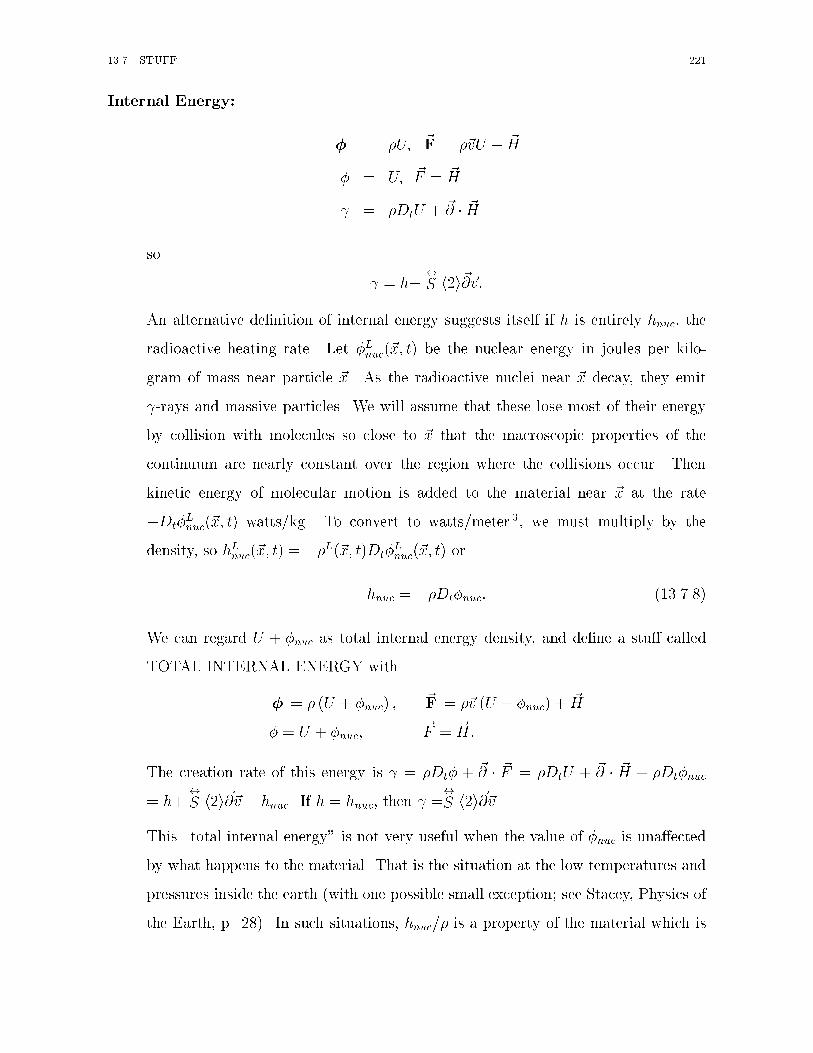
���� STUFF ���
Internal Energy�
� � �U� �F � ��vU � �H
� � U� �F � �H
� � �DtU � � � �H
so
� � h��
S hi��v�
An alternative de�nition of internal energy suggests itself if h is entirely hnuc� the
radioactive heating rate� Let �Lnuc��x� t� be the nuclear energy in joules per kilo�
gram of mass near particle �x� As the radioactive nuclei near �x decay� they emit
��rays and massive particles� We will assume that these lose most of their energy
by collision with molecules so close to �x that the macroscopic properties of the
continuum are nearly constant over the region where the collisions occur� Then
kinetic energy of molecular motion is added to the material near �x at the rate
�Dt�Lnuc��x� t� watts�kg� To convert to watts�meter �� we must multiply by the
density� so hLnuc��x� t� � ��L��x� t�Dt�Lnuc��x� t� or
hnuc � ��Dt�nuc� �������
We can regard U � �nuc as total internal energy density� and de�ne a stu� called
TOTAL INTERNAL ENERGY with
� � � �U � �nuc� � �F � ��v �U � �nuc� � �H
� � U � �nuc� �F � �H�
The creation rate of this energy is � � �Dt� � � � �F � �DtU � � � �H � �Dt�nuc
� h��
S hi��v � hnuc� If h � hnuc� then � ��
S hi��v�
This �total internal energy� is not very useful when the value of �nuc is una�ected
by what happens to the material� That is the situation at the low temperatures and
pressures inside the earth �with one possible small exception� see Stacey� Physics of
the Earth� p� ��� In such situations� hnuc�� is a property of the material which is

��� CHAPTER ��� CONSERVATION LAWS IN A CONTINUUM
known at any particle �x at any time t� independent of the motion of the continuum�
By contrast� the molecular U is not known at �x� t until we have solved the problem
of �nding how the continuum moves� In the deep interiors of stars� pressures and
temperatures are high enough to a�ect nuclear reaction rates� so it is useful to
include �nuc with U �
Kinetic Energy�
� ��
�v�� �F � ��v
��
v��� �
S ��v
� ��
v�� �F � � �
S ��v
� � �Dt�� � � �F ��
�Dtv
� � � ���
S ��v�
� ��v �Dt�v � i �Sijvj� relative to an orthonormal basis for P
� ��v � �a� �iSij� vj � Sijivj
����a� �� �S
�� �v� �
S hi��v
� � �f � �v� �
S hi��v�
IK Energy� �Internal plus Kinetic Energy��
This is the sum of internal energy and kinetic energy in the sense of de�nition
������� so it has
� � ����v� � U
�� �F � ��v
���v� � U
�� �H� �
S ��v� � �
�v� � U� �F � �H� �
S ��v� � h� �f � �v�
Potential Energy� Suppose the body force density �f is given by �f � ���� where
the potential function �E��r� t� is independent of time� i�e�� t� � �� Then Dt� �
t� � �v � �� � �v � �� so �Dt� � ��f � �v�
Then the stu� �potential energy� is de�ned by
� � �� �F � ��
� � ��� �F � ��v�

���� STUFF ���
so its creation rate is � � �Dt� � ��f � �v � ��
IKP Energy� �Internal plus kinetic plus potential energy��
If �f � ���� with t� � �� then we de�ne the stu� �IKP energy� as the sum of
internal� kinetic and potential energies in the sense of de�nition ��������� Then
� ��
v� � U � �� �F � �H� �
S ��v
� � ���
v� � U � �
�� �F � ��v
��
v� � U � �
�� �H� �
S ��v�
By corollary ������� � is the sum of the three ��s for kinetic� internal and potential
energy� so � � h� If we include nuclear potential energy in U and neglect other
sources of h �e�g� solar heating�� then � � �� Usually� this is not done� and IKP
energy is called �total energy��
������ Boundary conditions
So far we have dealt only with physical quantities which were continuously di�erentiable
to the extent needed to justify using Gauss�s theorem and the vanishing integral the�
orem� Now we analyze what happens when there is a surface S in the continuum� across
which physical quantities may have jump discontinuities� That is� lim�E��r� t� exists as �r
approaches �r� � S from either side of S� but the two limits are di�erent�
Examples of such surfaces are the interface between the ocean and atmosphere� the
ocean bottom� the core�mantle boundary� and a shock wave in air� water or rock� �Shock
waves in rock are excited only by nuclear blasts and meteor impacts� Earthquakes are
too weak to excite them��
We will assume that it is possible to choose a front side of S �M-obius strips are
excluded� and that we have done so� We will denote the unit normal to S on its front� or
positive� side by �� and we will call its back side the negative side� S is a large surface�
not nearly plane� but piecewise smooth� so � can vary with position �r � S� Moreover�
we will permit S to move� so that S�t� may vary with time t� Then so will ���r� t�� the
normal to S�t� at �r � S�t�� We will write W ��r� t� for the velocity with which S�t� moves

��� CHAPTER ��� CONSERVATION LAWS IN A CONTINUUM
. front+
back
^
r
r
S
ν( )
Figure �����
normal to itself at point �r � S�t�� and we take W � � if the motion is in the direction of
�� W � if opposite�
If the surface is given in physical space P � we write it as SE�t�� If it is given in label
space L� we write it as SL�t�� If � is any physical quantity with a jump discontinuity
across S�t�� we write �E��r�� t�� for the limiting value of �E��r� t� as �r �ro � SE�t� from
in front of SE�t�� We write �E��r�� t�� for the limit of �E��r� t� as �r �r� from behind
SE�t�� And we de�ne
h�E ��r�� t�
i��� �E��r�� t�
� � �E��r�� t��� �������
This quantity is called the jump in �E across SE�t�� We introduce a similar notation for
label space� with h�L ��x�� t�
i��� �L ��x�� t�
� � �L ��x�� t�� �
We will need the surface version of the vanishing integral theorem� This says that if
V is a Euclidean vector space� S is a surface in P or L� and �f � S V is continuous� andRS� dA��r�
�f��r� � �OV for every open patch S � on S� then �f��r� � �OV for all �r � S� Here an
�open patch� on S is any set S � � K � S� where K � is an open subset of P or L� The

���� STUFF ���
proof of the surface version of the vanishing integral theorem is essentially the same as
the proof of the original theorem ������� so we omit it�
We will consider only the Eulerian forms of the conservation laws� so we will omit the
superscript E� The reader can easily work out the Lagrangian forms of the law�
We use the notation introduced on page ��� but now we assume that the surface S�t�
passes through K ��t�� Therefore� we must augment the notation� We use K ��t�� for the
part �excluding S�t�� of K ��t� which is in front of S�t�� �K ��t� for the part of K ��t� in
front of S�t�� and K ��t�� for the whole boundary of K ��t��� including K ��t� S�t�� If �is a function de�ned and continuous on the closed set K ��t� � K ��t��K ��t�� except for a
jump discontinuity on S�t�� we write �� for the continuous function on K ��t�� de�ned as
� except on K ��t� S�t�� where its value is the �� of equation �������� We label objects
behind S�t� in the same way� except that � is replaced by �� The unit outward normal to
K ��t�� will be written n�� The unit outward normal to K ��t�� will be written n�� The
unit outward normal to K ��t� will be written n� Then n� � n on �K ��t� and n� � � �on K ��t� S�t�� And n� � n on �K ��t�� while n� � � on K ��t�S�t�� As on page ���
we choose K ��t� so that it always consists of the same particles� Then the outward normal
velocity of K ��t�� relative to itself is n ��� on �K ��t� and �W on K ��t�S�t�� Here �v is
the particle velocity in the continuum� The outward normal velocity of K ��t�� relative
to itself is n � �v on �K ��t� and W on K ��t� S�t��
������ Mass conservation
Let M �K ��t�� denote the mass of the material in K ��t�� Since K ��t� always consists of the
same particles� the physical law of mass conservation is
d
dtM �K ��t�� � �� ��������
We need a mathematical identity like �������� We begin with
M �K ��t�� �ZK�t�
dV ��r�� ��r� t� � ��������
This looks obvious until we recognize that there are physical situations which we might
want to model by placing a mass per unit area on S�t�� which would have to be added

��� CHAPTER ��� CONSERVATION LAWS IN A CONTINUUM
Figure �����

���� STUFF ��
to ��������� Examples are S�t� � the soap �lm in a soap bubble in air� or S�t� � the ice
pack on a polar sea� We ignore these possibilities and assume
mass on S�t� � �� �������
Next� we try to di�erentiate �������� using ��������� The jump discontinuity on
S�t� K ��t� prevents this� so we break �������� into
M �K ��t�� � MhK ��t��
i�M
hK ��t��
iwith �������
MhK ��t��
i�ZK�t��
dV ��r�����r� t� ��������
MhK ��t��
i�ZK�t��
dV ��r�����r� t�� ��������
The two integrands in �������� and �������� are continuous� so we can apply �������� to
obtain
d
dtMhK ��t��
i�ZK�t��
dV ��r� t���
Z��K�t�
dA n ��v����ZK�t��St�
dAW��� ��������
We would like to use Gauss�s theorem on the right in ��������� but �K ��t� is not a
closed surface�
To close it we must add K ��t� S�t�� ThenZ��K�t�
dA n � ���v�� �Z�K�t��
dA n� � ���v�� �ZK�t��St�
dA n� � ���v��
�ZK�t��
dV � � ���v�� �ZK�t��St�
dA � � ���v��
Using this in �������� gives
d
dtMhK ��t��
i�ZK�t��
dVht�� � � ���v�
i��ZK�t��St�
dA �� � � � v �W ��� �
But �t�� � � ���v��� in K ��t�� is just the value of t�� � � ���v� there� so it vanishes� and
d
dtMhK ��t��
i�ZK�t��St�
dA ��� � � �v �W ��� � ��������
By an exactly similar argument�
d
dtMhK ��t��
i�ZK�t��St�
dA ��� � � �v �W ��� � ��������

��� CHAPTER ��� CONSERVATION LAWS IN A CONTINUUM
Therefore�d
dtM �K ��t�� �
ZK�t��St�
dA ��� � � �v �W ���� � ��������
Combining �������� and �������� gives for K � � K ��t�
ZK�t��St�
dA ��� � � �v �W ���� � �� �������
Since K � can be any open subset of K�t�� K � S�t� can be any open patch on S�t��
Therefore� by the surface version of the vanishing integral theorem
�� � � � �v �W ���� � � on S�t�� �������
By analogy with de�nition ����� ii�� we call either ��� � ��v�W ��� or ��� � ��v�W ���
the �ux of mass across S�t�� and write it m��r� t� since it depends on �r and t� Thus
m � ��� ��v �W ��� � ��� ��v �W ��� � ������
If m � �� S�t� is a boundary between materials� It is then called a contact surface� It is
not crossed by particles� Then
� � �v � � � � �� � W� ������
If m �� �� S�t� is a shock wave or shock front�
������ Momentum conservation
Again refer to �gure ����� Let �P �K ��t�� be the momentum in K ��t�� while �F �K ��t�� is
the force on that material� Then mometum conservation requires
d
dt�P �K ��t�� � �F �K ��t�� � �������
We must �nd mathematical identities for the two sides of �������� Because of ��������
we have
�P �K ��t�� �ZK�t�
dV ��v� �������

���� STUFF ���
Again we cannot appeal directly to �������� to di�erentiate �������� because of the
jump discontinuity on S�t�� Therefore we imitate the procedure beginning on page ��
We have
�P �K ��t�� � �PhK ��t��
i� �P
hK ��t��
i�������
where
�PhK ��t��
i�ZK�t��
dV ���v�� �������
�PhK ��t��
i�ZK�t��
dV ���v��� �������
Then� appealing to ��������� we have
d
dt�PhK ��t��
i�
ZK�t��
dV t���v��
�Z��K�t�
dA n � ��v��v��
�ZK�t��St�
dAW ���v��
and
Z��K�t�
dA n � ��v��v�� �Z�K�t��
dA n� � ���v�v��
�ZK�t��St�
dA n� � ���v�v��
�ZK�t��
dV � � ���v�v��
�ZK�T ��St�
dA � � ���v�v�� �
Thus
d
dt�PhK ��t��
i�
ZK�t��
dVht ���v� � � � ���v�v�
i��ZK�t��St�
dA �� � � �v �W � ��v �� �
Now
t���v� � � � ���v�v� �ht�� � � ���v�
i�v � �
ht�v � �v � ��v
i� �Dt�v � ��a � �� �S ��f

��� CHAPTER ��� CONSERVATION LAWS IN A CONTINUUM
so� using Gauss�s theorem
d
dt�PhK ��t��
i�
Z�K�t��
dA n�� �S�
�ZK�t��
dV �f �ZK�t��St�
dA �� � � �v �W � ��v��
�ZK�t��
dV �f �Z��K�t�
dA n� �S
�ZK�t��St�
dA�� �� �S ��� � � �v��W � ��v
���
Using ����� we �nally get
d
dt�PhK ��t��
i�
ZK�t��
dV �f ��Z��K�t�
dA n� �S
�ZK�t��St�
dA�� �� �S �m�v
��� �������
An exactly similar argument gives
d
dt�PhK ��t��
i�
ZK�t��
dV �f �Z��K�t�
dA n� �S
�ZK�t��St�
dA�m�v � �� �S
��� �������
Therefore� adding ������� and ��������
d
dt�P �K ��t�� �
ZK�t�
dV �f �Z�K�t�
dA n� �S
�ZK�t��St�
dA�m�v � �� �S
���� �������
We still need a mathematical identity for �F �K ��t�� in �������� This seems easy�
�F �K ��t�� �ZK�t�
dV �f �Z�K�t�
dA n� �S � ������
But ������ does involve assumptions� If S�t� is an air�water interface holding an electric
charge per unit area� there will be an electrostatic force per unit area on S�t� which must
be added to ������� In addition� the surface integral on the right in ������ assumes
that the stress on the material just inside K ��t� by the material just outside K ��t�
is n� �S�
behind S�t� and n� �S�
in front of S�t�� all the way to S�t�� In fact� if S�t�
is an air�water interface� for example� the water molecules just behind S�t� and the air

���� STUFF ���
molecules just in front will be arranged di�erently from those in the bulk of the air and
water� Therefore� along the curve K ��t� S�t� there will be an additional force per unit
length exerted by the molecules just outside K ��t� on the molecules just inside K ��t��
This force per unit length is called the surface stress in S�t�� For an air�water interface it
is tangent to S�t� and normal to K ��t� S�t�� and its magnitude is the surface tension�
We assume
there is no surface stress or surface force per unit area on S�t�� ������
Then ������ is correct� and substituting ������� and ������ in ������� givesZK��St�
dA�m�v � �� �S
���� � �������
for any open subset K � of K�t�� By the surface version of the vanishing integral theorem�
it follows that �m�v � �� �S
���� � on S�t�� �������
If S�t� is a boundary between two materials rather than a shock� then m � � so
������� reduces to � �� �S
���� � on S�t�� �������
At a boundary between two materials �a contact surface�� the stress on the boundary �the
�normal stress�� is continuous across that boundary�
Equation ������� has a simple physical interpretation� Consider a small patch dA
on S�t�� Mass m�t dA crosses dA from back to front in time �t� and gains momentum
m�t ��v��� dA � �m�v��� �tdA� Therefore� the patch requires momentum to be supplied to
it at the rate �m�v���dA per second� Where does this come from$ In the material the
�ux density of momentum is � �
S� so momentum arrives at the back of dA at the rate
� �� �S�dA and leaves the front at the rate � �� �S
�dA� The net momentum accumulation
rate in dA� available to supply the required �m�v���dA� is � � ��
S� dA � � � �
S�
�dA
� � � ��S���dA� Thus ������� simply says that the di�erence in momentum �ux into the
two sides of dA supplies the momentum needed to accelerate the material crossing dA� If
m � �� this reduces to action � reaction� i�e� ��������

��� CHAPTER ��� CONSERVATION LAWS IN A CONTINUUM
����� Energy conservation
The physical law of conservation of energy is
d
dtE �K ��t�� �W �K ��t�� �������
where E �K ��t�� is the total kinetic plus internal energy in K ��t� and W�K ��t�� is the rate
at which energy is being added� We refer again to �gure ���� and follow the by now
well�trodden path to �nd mathematical identities for both sides of �������� We have
E �K ��t�� � EhK ��t��
i� E
hK ��t��
iwhere
EhK ��t��
i�ZK�t��
dV����
v� � U
����������
with a similar formula for E �K ��t���� Then
d
dtEhK ��t��
i�
ZK�t��
dV t
����
v� � U
����Z��K�t�
dA n ���v���
v� � U
����ZK�t��St�
dAW����
v� � U
����
Also
R��K�t� dA n �
h��v���v� � U
�i��R��K�t�� dA n� �
h��v���v� � U
�i�� RK�t��St� dA n� �
h��v���v� � U
�i��RK�t�� dV
� �h��v���v� � U
�i��RK�t��St� dA � �
h��v���v� � U
�i��
Thus�
d
dtEhK ��t��
i�
ZK�t��
dV�t
����
v� � U
��� � �
���v��
v� � U
�����ZK�t��St�
dA�� � � �v �W � �
��
v� � U
����
Now on page � we see that IK energy is a stu� with
, � ���
v� � U
�� �F � ��v
��
v� � U
�� �H� �
S ��v�

���� STUFF ���
Therefore t, � � � �F � � � h � �f � �v for this stu�� Thus th���
�v� � U�
i� � �h
��v���v� � U
�i� � � �H � � �
��
S ��v�� h� �f � �v� and
d
dtEhK ��t��
i�
ZK�t��
dV��� � �H � � �
��
S ��v�� h � �f � �v
���ZK�t��St�
dA m��
v� � U
���
ZK�t��
dV�h � �f � �v
���Z�K�t��
dA n� ��� �H�
�
S ��v��
�ZK�t��St�
dA m��
v� � U
��
d
dtEhK ��t��
i�
ZK�t��
dV�h� �f � �v
���Z��K�t�
dA n ��� �H�
�
S ��v�
�ZK�t��St�
dA�m��
v� � U
�� � �
��H� �
S ��v���
� �������
Similarly�
d
dtEhK ��t��
i�
ZK�t��
dV�h� �f � �v
���Z��K�t�
dA n ��� �H�
�
S ��v�
�ZK�t��St�
dA�m��
v� � U
�� � �
��H� �
S ��v���
� ��������
Therefore
d
dtE �K ��t�� �
ZK�t�
dV�h � �f � �v
��Z��K�t�
dA n ��� �H�
�
S ��v�
�ZK�t��St�
dA�m��
v� � U
�� � �
��H� �
S ��v���
�� ��������
Also�
W �K ��t�� �ZK�t�
dV�h� �f � �v
��Z�K�t�
dA n ��� �H � �S � �v
��
Therefore� ������� implies
ZK��St�
dA�m��
v� � U
�� � �
��H� �
S ��v���
�� � �������
for every open subset K � ofK�t�� By the surface version of the vanishing integral theorem��m��
v� � U
�� � � �H � �� �S ��v
���� � on S�t�� �������

��� CHAPTER ��� CONSERVATION LAWS IN A CONTINUUM
If the material is stationary� m � � and �v � �� so ������� reduces to the thermal
boundary condition h � � �H
i��� �� ��������
At a material boundary which is not a shock� m � �� so � �� �S �� � � �� �S��� and
� �� �S ��v��� � � �� �S�� � �v� �� �� �S�� � �v� � � �� �S� � ��v��� where �� �S� � �� �S�� � � �� �S���Also� from ������� if �v � v � � �vS where vv � � � �v� then v� � v� � so ��v��� � ��vS�
��
Therefore ������� becomes h � � �H
i���� �� �S
�� ��vS��� � ��������
The quantity � � � �H��� is the net heat �ow per unit area per second from the boundary into
the surrounding medium� Equation �������� says that heat is generated mechanically
when the two materials slip past one another at the relative velocity ��vS��� and when the
surface stress � �� �S� on the boundary has a component in the direction of the tangential
relative slip velocity� Brune� Henyey and Roy �J� Geophys� Res� ��� ��� used the
absence of an observed heat �ow anomaly along the San Andreas fault� together with an
estimate of ��vS��� on the fault� to put an upper bound on the component of �� �S in the
direction of slip� They used ���������
Even when m �� �� ������� can be made to resemble ������� We have��
mv�
���
��
m��v � � �v �
����v � � �v �
��
�
� ���
S� � �
S�����v � � �v �
�from �����
so ��
mv� � �� �S ��v
���
��
� ��� �
S� ��v �� �
S� ��v ��
�
S� � �v�� �
S� � �v�
�� � � � �
��
S��
�
S��� ��v��� �
De�ne
h�Si�� ��
��
S��
�
S��� average
�
S on S� ��������
Then ������� can be written in general ash � � �H �m U
i��� � � h�Si�� � ��v��� � ��������

Chapter ��
Strain and Deformation
��� Finite deformation
Consider a continuum which at time t occupies open subset K�t� of physical space P �
Suppose K ��t�� is a very small open subset of K�t��� We would like to be able to visualize
the particles in K ��t��� and to see their spatial positions at a particular later time t� The
time di�erence t � t� is not small� but K ��t�� is a very small set� in a sense to be made
precise shortly�
We use t��position labelling� Then label space L is the same as physical space P �
and �r L��x� t� � position at time t of the particle which was at position �x at time t�� The
particles in which we are interested have their labels in the set H � � K ��t��� First choose
a particular particle �xA � K ��t��� Let �rA be its position at time t� Then �rA � �r L��xA� t��
Consider any other particle �x � K ��t��� and let �r be its position at time t� Then �r �
�r L��x� t�� De�ne �� � �r � �rA� �� � �x� �xA� Then
�� � �r L��x� t�� �r L��xA� t� � �r L��xA � ��� t�� �r L��xA� t�
so
�� � �� � �D�r L ��xA� t� � k��k�R����
��������
where �R���� is the remainder function for �r L��� t� at �xA�
�

��� CHAPTER ��� STRAIN AND DEFORMATION
..
..
ξ
0
ρ
AAx
r
r
x
r
.( , t)
H =K (t ) K (t)
L
′ ′ ′
Figure �����
Now we assume that K ��t�� has been chosen so small that for every �x � K ��t���
k�R����k k �D�r L ��xA� t� k� �������
This is the sense in which K ��t�� must be a small set� If ������� is satis�ed� then we can
neglect the remainder term in �������� and write
�� � �� � �D�r L ��xA� t� � �������
If we measure initial positions in K ��t�� as displacement vectors from an origin at �xA�
and �nal positions in K ��t� as displacement vectors from an origin �rA� the mapping from
initial to �nal positions �� �� �� is linear� and is �������� Thus the e�ect of the motion
on the particles in K ��t�� is clear� The particle at �xA is displaced to �rA� The relative
positions of nearby particles� relative to particle �xA�s position� su�er the linear mapping
��������
As we have noted �see ������ j det �D�r L��xA� t��j is never � for any t�� But �r L�x� t�� �
�x� so �D�r L��x� t�� ��
I P and det �D�r L��xA� t�� � �� Then� since det �D�r L��xA� t�� depends
continuously on t� and is never �� it cannot change sign� so it is always positive� Therefore
det �D�r L ��xA� t� � �� ��������
It follows from the polar decomposition theorem �page D��� that there are unique tensors�
C and�
R� P � P with these properties�

����� FINITE DEFORMATION ��
i��
C is symmetric and positive de�nite�
ii��
R is proper orthogonal �i�e�� a rotation through some angle � between � and � about
some axis w��
iii�
�D�r L ��xA� t� ��
C � �R � ��������
Thus ������� is
�� � ��� �C � �R � ��������
Thus the e�ect of the motion on K ��t�� is to displace �xA to �rA� then to subject the relative
position vectors �relative to particle �xA� to the symmetric operator C� and then to rotate
everything through angle � about an axis passing through �rA in the direction of w�
The displacement �xA �� �rA and the rotation�
R are easy to visualize� The mapping�
C may be worth discussing� Since�
CT��
C there is an orthonormal basis y�� y�� y� for P
which consists of eigenvectors of C� That is� there are scalars c�� c�� c� such that
C � yi� � ci� yi�� i � �� � � ��������
Then yi��
C� ci� yi� so�
C��
I P ��
C� � yi yi� ��
C � yi
� yi�
�
C
��P�
i � ci� yi� yi�� Thus
�
C� c� y� y� � c� y� y� � c� y� y�� ��������
Since�
C is positive de�nite� c� and c� and c� must all be positive� Now �� � �� y���� y���� y�
so ��� �C� c��� y� � c��� y� � c��� y�� If we imagine a cube with edges of unit length parallel
to the axes y�� y�� y�� the e�ect of�
C is to multiply the i�th edge of the cube by ci�
transforming that cube to the rectangular parallelipiped in �gure ����
Suppose that in K ��t�� we imagine a small cube� with edges of length � parallel to the
axes y�� y�� y� which are eigenvectors for�
C� We can use the cube on the left in ��� by
shrinking its edges to � and placing the hidden vertex at �xA� Then the e�ect of �r L��� t�on this cube is
i� to translate it so the hidden vertex is at �rA�

��� CHAPTER ��� STRAIN AND DEFORMATION
^
^
^
y1
1
y3
1
1
y2
^
^
^
y
c
y
y
c
1
3
2
3
1
2
c
Figure ����

����� FINITE DEFORMATION ���
ii� to stretch or compress it by the factor ci in the direction yi� as shown in Figure ����
iii� to rotate it through angle �� with � � � � �� about an axis passing through �rA in the
direction w�
Now �������� implies
�D�r L ��xA� t� ��
R ��
C � ��������
where�
C ���
R�� � �C � �R��Xi �
ci
� yi�
�
R
�� yi�
�
R
�� ���������
Therefore we can perform the rotation�
R as step ii�� and the stretching or compression
as step iii�� But then� from ���������� the orthogonal axes along which stretching or
compression occurs are the rotated axes y���
R� y���
R� y���
R�
All this motivates the following de�nition�
De�nition ������ Suppose a continuum is labelled with t��positions� and �r L � K�t���R P is the resulting Lagrangian description of the motion� Suppose t � R� Then
�r L��� t� � K�t�� K�t� is called the �deformation� of the continuum from t� to t� For
any �xA � K�t��� �D�r L��xA� t� is the �deformation gradient� at particle �xA� The rotation�
R in �������� and �������� is called the �local rotation at particle �xA�� and�
C in ��������
is the �prerotation stretch tensor at �xA�� while�
C � in ���������������� is the �postrotation
stretch tensor at �xA�� We will write �D�r L��xA� t� as�
Gt�L��xA� t�� For any t��
�
Gt� � is a
physical quantity�
Various tensors obtained from�
C or�
C � are called �nite strain tensors� The commonest
is probably�
C � �
I P � and the most useful is probably
�Xi �
�ln ci� yi yi�
All these strain tensors reduce to the in�nitesimal strain tensor when the deformation is
nearly the identity mapping �see next section�� and to�� when �r L��� t� ��
I P �
In the foregoing discussion� the displacement of particle �xA to position �rA was so easy
to visualize that we said very little about it� It is worth considering� If we �x t�� the

��� CHAPTER ��� STRAIN AND DEFORMATION
displacement vector of any particle �x at time t is
�sL ��x� t� � �r L ��x� t�� �r L ��x� t�� � ���������
As the notation indicates� we will consider the physical quantity �s� called displacement�
whose Lagrangian description is the �sL de�ned by ���������� The de�nition requires that
we �x t�� If we change it� we change the de�nition of �s�
For t��position labelling� �r L��x� t�� � �x � �x L��x� t� so �sL��x� t� ���r L � �x L
���x� t��
Therefore
�s � �r � �x for t��position labelling� ��������
Equation �������� makes it convenient to use t��position labelling when studying dis�
placements� In particular� for such labelling� � �D�x �L��x� t� � �D�x ��
I P so �D�x ��
I P �
Thus� from ��������
�D�r ��
I P � �D�s for t��position labelling� ��������
Also� ���r �E��r� t� � ��r ��
I P so ��r ��
I P � Then from ��������
� �x ��
I P ���s for t��position labelling� ���������
But �� �x � � � �D�r � ��
I P � so from �������� and ���������� ��
I P ��
�s�� ��I P � �D�s� ��
I P � or�
I P � �D�s� ��s� ��s � �D�s ��
I P � or
�D�s � ��s� ��s � �D�s � ��s ���
I P � �D�s�� ���������
��� In�nitesimal displacements
We use t��position labelling throughout this section� and we discuss the displacement �s
de�ned by ��������� or ���������
De�nition ������ A tensor�
T� P � P is �small� if k �
T k �� That is k �
T hi �
T
k �� �� A tensor�
Q� P � P is �close to the identity� if�
Q � �
I P is small�

����� INFINITESIMAL DISPLACEMENTS ���
Remark ������ Suppose�
T� P � P and k �
T k �� De�ne ��
T �n ��
T n� so�
T ���
I P ��
T ���
T ��
T ���
T � �T ��
T ���
T � �T � �T � etc� Then ��
I P ��
T ��� and limN� PN
n �����n�
T n
both exist� and they are equal�
Proof�
kNX
n M
����n�
T n k �NX
n M
k �
T kn � k �
T kM�� k �
T k�
As M � N �� this �� so the Cauchy convergence criterion assures the
existence of limN� PN
n �����n�
T n� Then
��
I P ��
T
��
NXn �
����n �
T n �NXn �
����n �
T n �NXn �
����n�
T n��
�NXn �
����n�
T n �N��Xn �
����n�
T n��
I P �����N �
TN��
�
But k �
TN�� k � k �
T kN��� so letting N � on both sides gives
��
I P ��
T
�� Xn �
����n �
T n��
I P �
QED
Corollary ������� If k �D�sk �� then k��sk �� and to �rst order in �D�s�
�D�s � ��s� �������
Proof�
By remark �������� ��
I P � �D�s��� exists and equalsP
n �����n��D�s�n� Then
k��I P � �D�s���k � P n � k �D�skn � �����kD�sk�� By ��������� � ��s � �D�s � ��I P
� �D�s ���� so
k�sk � k �D�skk�IP � �D�s
��� k � k �D�sk� ��� k �D�sk� �

��� CHAPTER ��� STRAIN AND DEFORMATION
Remark ������ If�
T� P � P and�
T is symmetric and k �
T k �� then�
I P ��
T is
positive de�nite and its positive de�nite square root is
��
I P ��
T
�����
Xn �
�B� ��
n
CA �
T n ������
where �B� N
n
CA � N�N � �� � � � �N � n � ���n� �� � if n � ���
Proof�
If k �
T k �� all T �s eigenvalues lie between �� and �� Therefore�
I P ��
T has
all its eigenvalues between � and � Therefore� it is positive de�nite� ThatP n �
����n�
�
T n exists� is positive de�nite� and when squared gives�
I P ��
T
can be proved in the same way as remark ��������� Alternatively� the e�ect
ofPN
n �
����n�
�
T n can be studied on each of the vectors in an orthonormal
basis for P consisting of eigenvectors of�
T � Then one simply uses the known
validity of ������ when�
I P is replaced by � and�
T by any of its eigenvalues�
Corollary ������� Suppose�
T T��
T and k �
T k �� Then correct to �rst order in k �
T k���
I P ��
T
������
I P ��
�
T �
Theorem ������ Use the notation of de�nition ��������� and de�ne the displacement �s
by ��������� Suppose that k �D�sk �� Then to �rst order in �D�s we have
��s � �D�s ������
�
C��
C���
I P ��
h�D�s ��xA� t� � �D�s ��xA� t�
Ti
�������
�
R��
I P ��
h�D�s ��xA� t�� �D�s ��xA� t�
Ti� �������
Proof�

����� INFINITESIMAL DISPLACEMENTS ���
We have already proved ������� For the rest� abbreviate �D�s��xA� t� as�
T �
Since �D�r ��
C � �R we have � �D�r � � � �D�r �T ��
C � �R ��
RT ��
CT ��
C � �R ��
R��
� �C��
C � �I P ��
C��
C�� so
�
C ����D�r
����D�r
�T �����
���
I P ��
T
����
I P ��
T T
�����
�
��
I P ��
T ��
T T ��
T ��
T T
����
��
I P ��
��
T ��
T T ��
T ��
T T
��O
�k �
T ��
T T ��
T ��
T T k��
��
I P ��
��
T ��
T T
��O
�k �
T k���
Also� �D�r ��
R ��
C �� so��D�r
�T � ��D�r��
�
C �T ��
RT � �R ��
C � ��
C � ��
R�� � �R ��
C �
��
C � � �I P ��
C ����
C �
��so
�C � ����D�r
�T � � �D�r�����
�
���
I P ��
T T
����
I P ��
T
�����
�
��
I P ��
T T ��
T ��
T T � �T�
��
I P ��
��
T T ��
T ��
T T � �T��O
�k
�
T T ��
T ��
T T �� �T k��
��
I P ��
��
T ��
TT��O
�k �
T k���
Finally��
R��
C�� � �D�r ��
C�� ���
I P ��
T
�and
�
C����
I P ���
��
T ��
T T
��O
nk�Tk�
oso
�
R �
��
I P ��
��
T ��
T T
��O
nk�Tk�
o����
I P ��
T
�
��
I P ��
��
T ��
T T
��O
nk�Tk�
o�
QED�
De�nition ������ Use t��position labelling so the displacement �s is de�ned by ���������
Suppose k �D�sL��x� t�k �� Then the tensor
��L��x� t� �
�
h�D�sL��x� t� � �D�sL��x� t�T
i�������

��� CHAPTER ��� STRAIN AND DEFORMATION
is called the in�nitesimal strain tensor at particle �x at time t� and
�
wL ��x� t� ��
h�D�sL��x� t�� �D�sL��x� t�T
i�������
is the in�nitesimal rotation tensor� The vector
�wL ��x� t� ��
AP hi �
wL��x� t� �������
is called the in�nitesimal rotation vector at particle �x at time t�
Corollary ������� �wL��x� t� can be written �� �D��sL��x� t� or ���� � �s
�L��x� t� because
�wL ��x� t� ��
AP hi �D�sL ��x� t� �������
and� to �rst order in �D�s�
�wL ��x� t� ��
AP hi
���s�L
��x� t� � ��������
Proof�
�������� follows from ������� and ������� To prove ������� note that for
any tensor�
T we have
AP hi�
T T� �AP hi�
T � ��������
To see this� look at components relative to a pooob in P � Then ��������
is equivalent to �ijkTkj � ��ijkTjk� But by changing index names we get
�ijkTkj � �ijkTjk � ��ijkTjk� Applying �������� to ������� ������ with�
T� �D�sL��x� t� gives �������� QED
Corollary ������� Let y�� y�� y� be an orthonormal basis for P consisting of eigenvectors
of�� ��xA� t�� where �xA is as in de�nition ������� Then to �rst order in �D�sL��xA� t��
�
C��
C���
I P ��� ��xA� t� �
�Xi �
�� � �i� yi yi �������
where ��� ��� �� are the eigenvalues of�� ��xA� t� belonging to the eigenvectors y� � y�� y��
And�
R is a rotation in the right�handed�screw sense through angle k�wL��xA� t�k about theaxis through �OP in the direction �wL��xA� t��

����� INFINITESIMAL DISPLACEMENTS ���
δφ
ω
ξ sin θ
ξ
ω ξx
OP
θ
Figure ����
Proof�
We show�� ��xA� t� �
P�i � �i yi yi in the same way we showed ��������� The
rest of ������� follows from �������� To prove the results about�
R� we note
from exercise �c that
�wL��xA� t� � AP � �wL ��xA� t� �
Then from �������� to �rst order in �D�s
�
R��
I P �AP � �wL��xA� t��
If we apply�
R to a vector ��� the result is
��� �R� �� � �� � AP � �wL ��xA� t� �
We claim �� � AP � �v � �v � ��� Looking at components relative to a pooob�
��� � Ap � �v�i � �j�jikvk � �ikjvk�j��v � ��
�i� Therefore
��� �R� �� � �wL ��xA� t�� ��� �������
Abbreviate �wL ��xA� t� by �w� and examine �gure ��� where �� � �R � ��� �w� ���
Since k�w � ��k � k�wkk��k sin �� clearly �� � k�wk� QED�

��� CHAPTER ��� STRAIN AND DEFORMATION
Now suppose
t � t� � �t ��������
where �t is small enough that it is a good approximation to write
�r L ��x� t� � �r L ��x� t�� � �tDt�rL ��x� t�� �O ��t�� � ��������
Then� since Dt�r � �v and �sL��x� t� � �r L��x� t�� �r L��x� t��� we have
�sL ��x� t� � �t�vL ��x� t�� �O ��t�� ��������
Then� to �rst order in �t�
��L��x� t� �
��L��x� t� � �t� � �t
�
h�D�vL ��x� t�� � �D�vL ��x� t��
Ti
��������
�wL��x� t� �
�wL��x� t� � �t� � �t
�
h�D�vL ��x� t��� �D�vL ��x� t��
Ti
��������
�wL��x� t� �
�wL��x� t� � �t� � �t
�
Aphi
h�D�vL ��x� t��
i� �t
�
�D � �vL ��x� t�� � ��������
Consider the material near particle �xA at various times t�� �t� with small �t� Relative to
particle �xA� the material stretches as in �������� the fractional stretching �i being propor�
tional to �t� �i � #�i�t� where #�i is one of the eigenvalues of ��h�D�vL ��xA� t�� � �D�vL ��xA� t��
Ti�
and yi in ������� is the corresponding eigenvector� And relative to particle �xA� the mater�
ial also rotates through angle �tk���D��vL��xA� t�k about an axis through �xA and in direction
���D��vL��x�� t�� In other words� it rotates with angular velocity �� �D��vL��xA� t�� To �rst
order in �t�
C ���
C� so the rotation can occur before or after the stretching� We prefer to
think of them as occurring simultaneously� The foregoing analysis began by choosing a
time t� at which to introduce t��position labels� We can choose t� to be any time we like�
the foregoing results are true for all t� � R� Therefore� we can de�ne physical quantities��� �
��w� #�w by requiring for any �x � P and any t� � r that
���E
��x� t�� ��
h�D�vL ��x� t�� � �D�vL ��x� t��
Ti
�������

����� INFINITESIMAL DISPLACEMENTS ��
��wE
��x� t�� ��
h�D�vL ��x� t��� �D�vL ��x� t��
Ti
�������
��wE
��x� t�� ��
�D � �vL ��x� t�� � ������
Here it is understood that to evaluate the left side of ������� ������ ����� at any
particular t�� we use that t� to establish t��position labels in establishing the Lagrangian
descriptions needed on the right� Each t� on the left calls for a new Lagrangian description
on the right� the one using t��position labels�
But with t��position labels� �D�r L��x� t�� ��
I P � so �EfE��x� t�� � �DLfL��x� t�� for any
physical quantity f � Therefore �D�vL can be replaced by ��vE on the right in ������ Since
the Eulerian description of physical quantities are independent of the way particles are
labelled� this replacement leads to the conclusions
����
�
���v �
���v�T �
������
��w�
�
���v �
���v�T �
�������
#�w ��
� � �v� �������
The quantity #�w is called the vorticity� and��� is the strain�rate tensor�

��� CHAPTER ��� STRAIN AND DEFORMATION

Chapter ��
Constitutive Relations
��� Introduction
Let us examine the conservation laws as a system� They are
Eulerian Form Lagrangian Form
Mass Dt�� �� � �v � � Dt � � � ��������
Momentum �Dt�v � �� �S ��f �Dt�v � �D�� S �� f �������
Internal Energy �DtU � � � �H � h��
S hi�v �DtU � �D � � H � h�� S hi �D�v�
�������
If we knew the initial values of �� �v and U � or �� �v and U � at some instant t�� we might
hope to integrate ������� forward in time to �nd later values of these quantities� To do
this� clearly we must know �f and h� or � f and h� and we will assume henceforth that these
are given to us� But there still remains the question of �nding �H and�
S� or� H and
� S� The
equations which give their values when the state of the material is known are called the
�constitutive equations� of the material� Ideally� we would like to be able to deduce these
from the molecular pictures of matter� but theory and computational techniques are not
yet adequate to this task for most materials� We must rely on experimental measurements�
The outcomes of these experiments suggest idealized mathematical models for various
classes of real materials�
��

��� CHAPTER ��� CONSTITUTIVE RELATIONS
K
n
K
∂
Figure �����
In modelling a real material� one usually begins by considering its homogeneous ther�
mostatic equilibrium states �HTES�� Then one studies small deviations from thermostatic
equilibrium� by linearizing in those deviations� Large deviations from thermodynamic
equilibrium are not fully understood� and we will not consider them� They make plasma
physics di!cult� for example�
A homogeneous thermostatic equilibrium state �HTES� is said to exist in a material
when no macroscopically measurable property of that material changes with time� and
when the macroscopic environments of any two particles are the same� The second law of
thermodynamics then implies that there can be no heat �ow in the material� The material
can have a constant velocity� but if it does we study it from a laboratory moving with
the same velocity� so we may assume �v � �� in an HTES� Then DtU � tU � But tU � �
so� from �������� h � �� The Cauchy stress tensor�
S must be the same everywhere at all
times in an HTES� so �� �S� ��� and ������ �momentum�� implies �f � ��� Therefore� in an
HTES we have
� � constant� �H � �� �v � ���
U � constant� h � ��
S� constant� �f � ��
If the material occupies a volume K with boundary K and unit outward normal n�
then in order to maintain the material in an HTES we must apply to the surface K a

����� INTRODUCTION ���
stress n� �S� and we must prevent surface heat �ow and volume heating� That is we need�������������surface stress applied to K at �r is n��r�� �S n��r� � �H � � at every �r � K
h � � at every �r � K�
��������
Two HTES�s are di�erent if they di�er in any macroscopically measurable quantity�
including chemical composition� Most pure substances require only the values of a few of
their physical properties in order to specify their HTES�s� For example� two isotropically
pure samples of H�O �no deuterium� only O��� liquid which have the same density and
the same internal energy per unit mass will have the same values of pressure� temperature�
entropy per gram� electrical resistivity� index of refraction for yellow light� neutron mean
absorption length at �� kev� etc� For water� the set of all possible HTES�s is a two�
parameter family� �We have ignored� and will ignore� electrical properties� It is possible
to alter U for water by polarizing it with an electric �eld��
Changes from one HTES to another are produced by violating some of the conditions
��������� Changes produced by altering the surface stress applied to K are said to �do
work�� while changes produced by letting h �� � are said to involve �internal heating or
cooling�� and n � �H �� � on K involves �heat �ow at K�� For the materials in which
we are interested� these changes can be described as follows� We pick one HTES as a
reference state� and call it HTES� We use t��position labelling� where t� is any time when
the material is in HTES�� We carry out a change by violating ��������� and wait until time
t� when the material has settled into a steady state� HTES�� The Lagrangian description
of the motion is �r L��x� t�� and it is independent of t for t � t� and for t � t�� We write
�r �� ��x� � �r L ��x� t�� � ��������
�
G�� ��x� � �D�r �� ��x� � ��������
Since the environments of all particles must be alike in HTES�� they must have been
subjected to the same stretch and the same rotation so
�
G�� is constant� independent of �x� ��������

��� CHAPTER ��� CONSTITUTIVE RELATIONS
��
G�� is called the deformation gradient of HTES� relative to HTES��� Then from ���������
�r ����x� � �x� �G�� ��r ������� If �r ������ �� ��� we may move the material with a uniform
displacement so �r ������ � ��� Thus we may assume
�r ����x� � �x� �G�� � ��������
Here �x is particle position in HTES� and �x� �G�� is particle position in HTES�� If we
want to study another HTES� say HTES�� we can adopt either HTES� or HTES� as the
reference state� If we use HTES� for refrence� then particle position in HTES� is �x���
G��
where �x� is particle position in HTES� and�
G�� is calculated from �������� but with t�
position labelling� If a particle has position �x in HTES�� then �x� � �x� �G�� and so �x� �
position in HTES� � �x���
G�� � �x� �G�� ��
G��� But also �x� � �x� �G��� so
�
G����
G�� ��
G�� ��������
for any HTES�� HTES�� HTES��
��� Elastic materials
The observed HTES�s of many material are approximated well by the following idealiza�
tion�
De�nition ������� An elastic material is one whose HTES�s have these properties�
i� If HTES� is any HTES� there is an M� � � such that for any�
G� P � P with k �
G
� �
I P k M�� there is an HTES� whose deformation gradient relative to HTES� is�
G����
G �
ii� Once a reference state HTES� is chosen� any other equilibrium state HTES� is com�
pletely determined by its deformation gradient�
G�� relative to HTES�� and by its
entropy per unit mass N��
iii� U � the internal energy per unit mass� is unchanged by rigid rotations� That is� if�
G� P � P and�
R� "��P � then
U��
G�N�� U
��
G � �R�N�� �������

����� ELASTIC MATERIALS ���
Now consider two di�erent HTES�s of an elastic material� say HTES� and HTES��
neither of them the reference state HTES�� Suppose �rL � K��R P is the Lagrangian
description of the motion which carries the material from state � to state � Here K� is
the region occupied by the material in HTES�� so the total mass of the material is
M � jK�j � ������
where jK�j � volume of K�� The total internal energy of the material is
U i � MUi � jK�j �Ui in HTESi� ������
Let ��W be the work done on the material and ��Q the heat added to it in going from
HTES� to HTES�� Energy conservation requires
��W � ��Q � U � � U �� �������
Now suppose HTES� and HTES� are not very di�erent� Then we will write df � f��f�for any property f of the two states� Thus ������� is dU � ��W � ��Q� According
to the second law of thermodynamics� correct to �rst order in small changes�
��Q � �dN � ��N � � N �� �������
where N i � jK�j �Ni � total entropy of state i� and � is the smaller of �� and ��� It
is possible to �nd processes �r L in which equality is approximated arbitrarily closely in
�������� These are called �reversible processes�� In such processes
��Q � �jK�j �dN� �������
In any transition from state � to state � reversible or not�
�DtU � � �D � � H � h�� S hi �D�v
so� integrating over K� and using Gauss�s theorem�
�ZK�
dVL��x�DtU �ZK�
dVL h�Z�K�
dAL nL � �H �ZK�
dVL� S hi �D�v

��� CHAPTER ��� CONSTITUTIVE RELATIONS
ord
dtU � #Q�
ZK�
dVL �Shi �D�v
where #Q is the rate at which heat is added to the material� Thus� integrating from t� to
t�
U � � U � � ��Q�Z t�
t�dtZK�
dVL� S hi �D�v�
Comparing with ������� we see that
��W �Z t�
t�dtZK�
dVL� S hi �D�v�
Now if the transformation is done slowly�� S will be nearly constant� about equal to its
value in HTES� or HTES� so
��W �� S hi
ZK�
dVL
Z t�
t�dt �D�v�
But �v � dt�r so �D�v � �DDt�r � � �D�v�L��x� t� � �DDt�r
L��x� t� � Dt�D�r L��x� t�
� �Dt
�
G�L��x� t�� Thus� �D�v � Dt
�
G� and
��W �� S hi
ZK�
dVL��x���
G ��x� t����
G ��x� t����
But�
G ��x� t�� and�
G ��x� t�� refer to HTES�s� They are independent of �x� Thus
��W � jK�j� S hid �
G � �������
From �������� ������� and �������� dU � jK�j� S hid �
G �jK�j ��dN � Since
dU � jK�j �dU � dividing by jK�j � gives
dU � d�
G hi� S
�� �dN �������
for small reversible changes between HTES�s� Here � and� S refer to either the initial or
the �nal state� since they are close�
But U is a function of�
G and N � Equation ������� says this function is di�erentiable�
and that
���
G�N��
NU��
G�N�
�������

����� ELASTIC MATERIALS ���
� S �
�
G�N�
�� ��
GU��
G�N�� ��������
where ��GU�
�
G�N� is an abbreviation forh�U��� N�
i� �G�� Since P�P is a Euclidean space�
the theory of such gradients is already worked out� In particular� if y�� y�� y� is a pooob
for P � then the dyads yi yj are an orthonormal basis for P � P � and
�
G� Gij yi yj� ��������
Then
�GU��
G�N�� yi yj
U��
G�N�
Gij
so� from �������� Sij�
�U�
�
G�N�
Gij� �������
To obtain the Cauchy stress tensor we use ������� namely
���
S
�
A ��
GT ��B�� S
�
CA � �������
The equation
U � U��
G�N�
��������
is called the equation of state of the elastic material� It can be solved for N as a function
of�
G and U �
N � N��
G�U�� ��������
This serves as the basis for
De�nition ������� A perfectly elastic material is one in which the small region near
any particle �x at any time t behaves as if it were in an HTES with�
G� �D �r L��x� t� and
U � UL��x� t��
In a perfectly elastic material� we will have �see page ��� h � �� �H � ��� and� S will be
given by ��������� so the missing information needed to integrate �������� ������ ������
is supplied by �������� which is known if the equation of state is known�
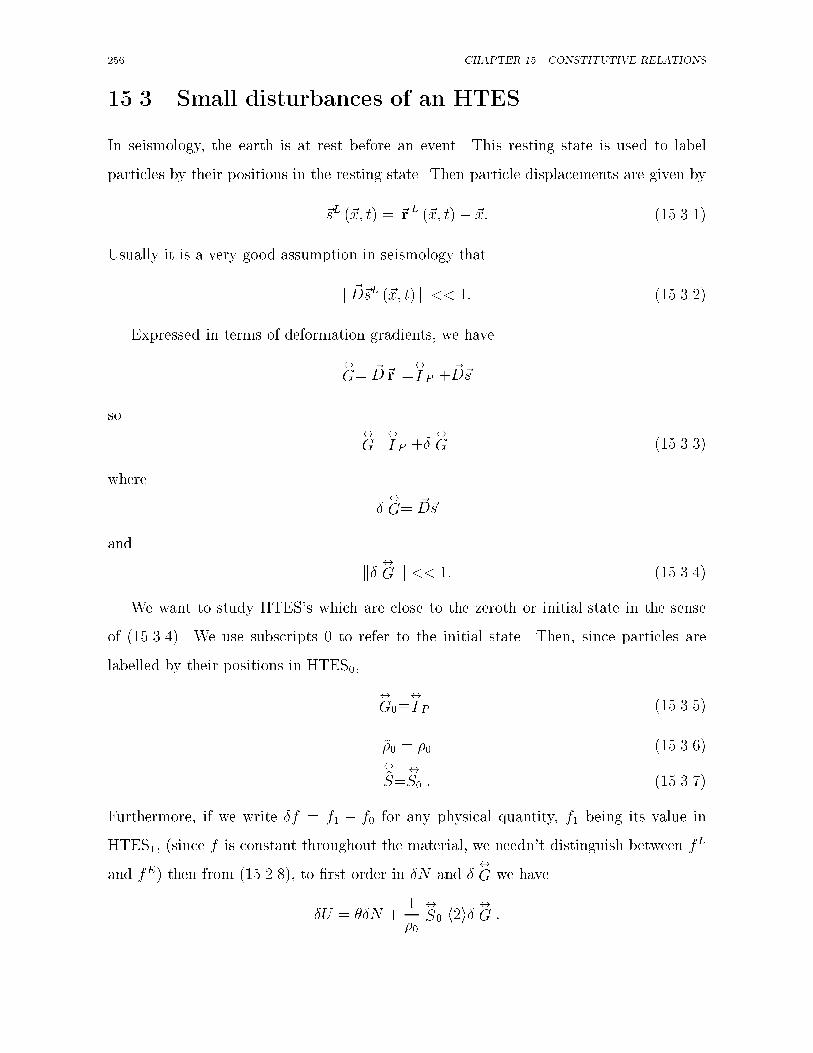
��� CHAPTER ��� CONSTITUTIVE RELATIONS
��� Small disturbances of an HTES
In seismology� the earth is at rest before an event� This resting state is used to label
particles by their positions in the resting state� Then particle displacements are given by
�sL ��x� t� � �r L ��x� t�� �x� �������
Usually it is a very good assumption in seismology that
k �D�sL ��x� t� k �� ������
Expressed in terms of deformation gradients� we have
�
G� �D�r ��
I P � �D�s
so�
G��
I P ���
G ������
where
��
G� �D�s
and
k� �
G k �� �������
We want to study HTES�s which are close to the zeroth or initial state in the sense
of �������� We use subscripts � to refer to the initial state� Then� since particles are
labelled by their positions in HTES��
�
G���
I P �������
�� � �� �������� S�
�
S� � �������
Furthermore� if we write �f � f� � f� for any physical quantity� f� being its value in
HTES�� �since f is constant throughout the material� we needn�t distinguish between fL
and fE� then from �������� to �rst order in �N and ��
G we have
�U � ��N ��
��
�
S� hi��
G �

����� SMALL DISTURBANCES OF AN HTES ��
If ��
GT� �� �
G� then�
G��
I P ���
G is a rotation to �rst order in ��
G� and therefore �N � �
implies �U � �� Consequently�
�
S� hi��
G� � if ��
GT� �� �
G �
But then for any ��
G��
S� hi���
G ���
GT
�� �� so
��
S� ��
S�T�hi� �
G� �� Thus
�
S���
ST� � �������
The Cauchy stress tensor is symmetric in every HTES of an elastic material�
We can go further� Since HTES� is close to HTES�� all the changes �f are small� so
we can linearize ������� and �������� The changes �� � �� � ��� �� S�
� S� �
� S�
are
given in terms of �N � N� �N� and ��
G��
G� ��
G� by
�� � �N���
G�� N�
�N
� ��
G hi��G���
G�� N�
�
� �S � �N
�S
��
G�� N�
�N
� ��
G hi�G
�S
��
G�� N�
��
We de�ne the following tensors�
�
�
Q�� ��P ��
W �� ��P � B� � R�
�
�
Q�� ��G
�S
��
G�� N�
�� ����
G��GU��
G�� N�
��������
�
W � �
N
�S
��
G�� N�
�� �
N��GU��
G�� N�
�� ���
G
NU��
G�� N�
�� ����
G����
G�� N�
���������
B� �
N���
G�� N�
��
�
N�U��
G�� N�
�� ��������
Then
�� � �NB� � ��
G hi�� �
W �
��
A �������
�Note� � � ��� Also
�� S� �N
�
W � ���
G hi��
Q� � �������

��� CHAPTER ��� CONSTITUTIVE RELATIONS
Furthermore� if y�� y�� y� is any pooob for P � and we write�
G as in �������� and write
��
Q�� Qijkl yi yj yk yl�
then
Qijkl � �U�GijGkl � �U�GklGij
so
Qijkl � Qklij or ������
��
Q��
��
Q� � ��������
We would also like to calculate ��
S��
S� ��
S�� the change in the Cauchy stress tensor�
From ������� and �������
�
S������det �G��
������ �
GT�� �
�
S��
Now det�
G �t� depends continuously on t in going from HTES� to HTES�� and can never
vanish� It is � in HTES�� so is always � �� Hence j det �G j � det�
G and
�
S���det
�
G��
��� �
GT�� �
�
S�� ��������
Now�
G����
G��
I P ���
G and� taking components relative to y�� y�� y�
det�
G �
������������ � �G�� �G�� �G��
�G�� � � �G�� �G��
�G�� �G�� � � �G��
������������ � � �Gii �O
�k� �
G k��� � � tr �
�
G �Ok �� Gk��
Thus �det
�
G
���� �� tr �
�
G �O�k� �
G k��� ��������
Then�
S����� tr �
�
G
���
I P ���
GT
����
S� �� �S
��
where we have used �������� and have linearized in ��
G� Keeping only terms up to �rst
order in ��
G� we have
�
S���
S� � �tr ��G���
S� ���
GT � �S� �� �S�

����� SMALL DISTURBANCES OF AN HTES ���
or
��
S� � �S � �
�
GT � �S� ��
S�
�tr �
�
G
�� ��������
If we take components relative to the pooob� y�� y�� y� from P � and write
�
S�� Sij yi yj ��������
then �������� becomes
�Skl � � Skl � �GikSil � �GjjSkl
� ��Gij�Qijkl � �NWkl � �Gij ��jkSil � �ijSkl�
� ��Gij� �Qijkl � Sil�kj � �ijSkl� � �NWkl�
We de�ne a tensor��
F� ��P by
��
F �� �Qijkl � Sil�kj � �ijSkl� yi yj yk yl�
or���
F ��
��
Q� ������
S�
�
I P
�� �
I P�
S� � ��������
Then
Fijkl � Qijkl � Sil�kj � �ijSk �������
and
��
S� ��
G hi��
F � ��N�
W � � �������
This equation is of exactly the same form as �������� but
��
Q� is replaced by��
F ��
Now ��
S is the di�erence between the Cauchy stress tensors in two HTES�s� so ��
ST�
��
S for any ��
G whatever and any �N � First� take ��
G� �� Then we must have
�
WT
���
W � � ������
Next� take �N � �� Then
�Skl � �GijFijkl � �Slk � �GijFijlk�
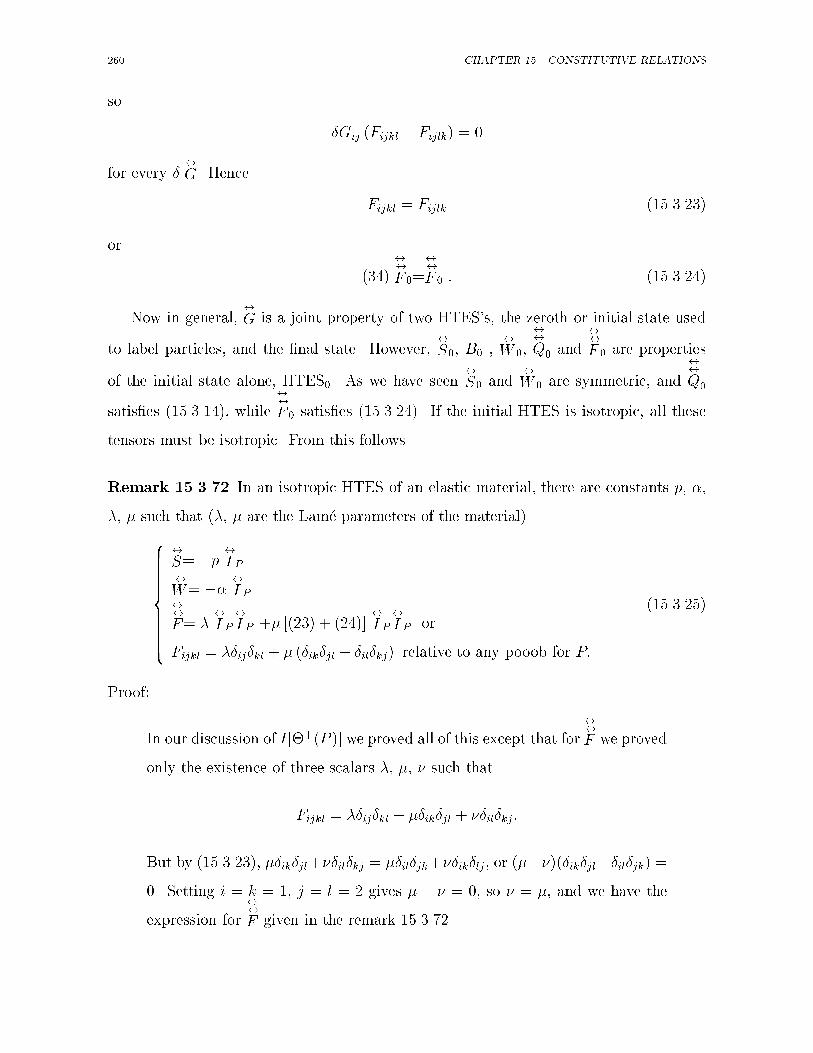
��� CHAPTER ��� CONSTITUTIVE RELATIONS
so
�Gij �Fijkl � Fijlk� � �
for every ��
G� Hence
Fijkl � Fijlk ������
or
���
��
F ��
��
F � � �������
Now in general��
G is a joint property of two HTES�s� the zeroth or initial state used
to label particles� and the �nal state� However��
S�� B� ��
W ��
��
Q� and��
F � are properties
of the initial state alone� HTES�� As we have seen�
S� and�
W � are symmetric� and
��
Q�
satis�es ��������� while��
F � satis�es �������� If the initial HTES is isotropic� all these
tensors must be isotropic� From this follows
Remark ������ In an isotropic HTES of an elastic material� there are constants p� ��
� � such that �� � are the Lam.e parameters of the material����������������������
�
S� �p �
I P�
W� �� �
I P��
F� �
I P�
I P �� ��� � �����
I P�
I P or
Fijkl � �ij�kl � � ��ik�jl � �il�kj� relative to any pooob for P�
�������
Proof�
In our discussion of I�"��P �� we proved all of this except that for��
F we proved
only the existence of three scalars � �� � such that
Fijkl � �ij�kl � ��ik�jl � ��il�kj�
But by ������� ��ik�jl���il�kj � ��il�jk���ik�lj� or �������ik�jl��il�jk� ��� Setting i � k � �� j � l � gives � � � � �� so � � �� and we have the
expression for��
F given in the remark ������

����� SMALL DISTURBANCES OF AN HTES ���
Corollary ������� For HTES�s close to an isotropic HTES��������� � ��N�B �
�tr
��������
��
S� �tr
��� �
I P �u��
�������
where��� ����
�
G ���
GT � � ����D�s�
��D�s�T�
� in�nitesimal strain tensor�
In most cases� the HTES� of the elastic material is not isotropic� either because the
material itself is anisotropic or because�
S� is anisotropic� Then the sti�ness tensor��
F �
gives the response of�
S to small changes ��
G in the deformation gradient�
G away from�
G���
I P � The sti�ness tensor has two sets of symmetries �see ������
Fijkl � Fijlk� �������
The second symmetry is obtained �������� and �������� Let
Rijkl �� �jkSil � �ijSkl� �������
Then from ������� Qijkl � Fijkl � Rijkl� so from ��������
Fijkl � Fklij �Rijkl � Rklij� �������
Since Fijkl have to be measured experimentally� and there are �� such components� we
would like to use ������� and ������� to see how many of these components are ind�
pendent� Only those need be measured and recorded�
To answer this question we need one more symmetry� deducible from ������� and
�������� We have from those two equations
Fijkl � Fklji �Rijkl � Rklij�
Interchange i and j in �������� so
Fkljk � Fjikl � Rjikl �Rklji�
Then
Fijkl � Fjikl �Rijkl � Rklij �Rklji �Rjikl� �������

��� CHAPTER ��� CONSTITUTIVE RELATIONS
Now de�ne
��
E�� ��P by
Eijkl ��
��Fijkl � Fjikl � Fklij � Flkij� � �������
Then it is a trivial algebraic identity that
Fijkl � Eijkl ��
��Fijkl � Fijkl� �
�
��Fijkl � Fjikl�
��
��Fijkl � Fklij� �
�
��Fijkl � Flkij�
� Eijkl ��
��Fijkl � Fjikl� �
�
��Fijkl � Fklij�
��
��Fijkl � Fklij � Fklij � Flkij�
� Eijkl ��
��Fijkl � Fjikl� �
�
�Fijkl � Fklij�
��
��Fklij � Flkij� �
Using ������� once as written and once with the interchanges i ! k and j ! l� and
using ������ once as written� we get
Fijkl � Eijkl ��
��Rijkl �Rklij �Rklji � Rjikl�
��
��Rklij � Rijkl �Rijlk �Rlkij�
��
�Rijkl � Rklij�
� Eijkl ��
�Rijkl �Rklij� �
�
��Rijlk � Rlkij�
��
��Rjikl �Rklji�
� Eijkl ��
��jkSil � �ijSkl � �liSkj � �klSij�
��
���jlSik � �ijSlk � �kiSlj � �lkSij�
��
���ikSjl � �jiSkl � �ljSki � �klSji� �
Therefore
Fijkl � Eijkl ��
��klSij � �ijSkl � �jlSik � �ikSjl � �jkSil � �ilSjk� ������
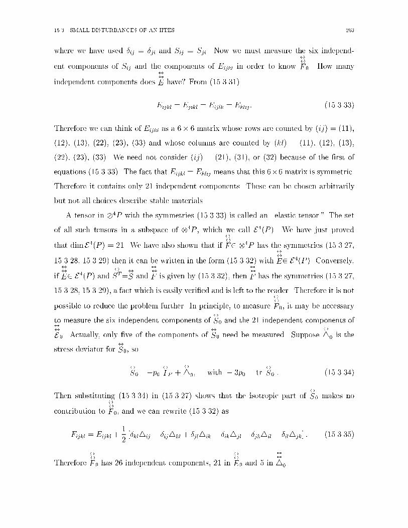
����� SMALL DISTURBANCES OF AN HTES ���
where we have used �ij � �ji and Sij � Sji� Now we must measure the six independ�
ent components of Sij and the components of Eijkl in order to know��
F �� How many
independent components does
��
E have$ From �������
Eijkl � Ejikl � Eijlk � Eklij� ������
Therefore we can think of Eijkl as a �� � matrix whose rows are counted by �ij� � �����
���� ���� ��� ��� �� and whose columns are counted by �kl� � ����� ���� ����
��� ��� ��� We need not consider �ij� � ���� ���� or �� because of the �rst of
equations ������� The fact that Eijkl � Eklij means that this ��� matrix is symmetric�
Therefore it contains only � independent components� These can be chosen arbitrarily
but not all choices describe stable materials�
A tensor in ��P with the symmetries ������ is called an �elastic tensor�� The set
of all such tensors in a subspace of ��P � which we call E��P �� We have just proved
that dimE��P � � �� We have also shown that if
��
F� ��P has the symmetries �������
������ ������ then it can be written in the form ������ with
��
E� E��P �� Conversely�
if
��
E� E��P � and�
ST��
S and
��
F is given by ������� then
��
F has the symmetries �������
������ ������� a fact which is easily veri�ed and is left to the reader� Therefore it is not
possible to reduce the problem further� In principle� to measure
��
F �� it may be necessary
to measure the six independent components of�
S� and the � independent components of��E �� Actually� only �ve of the components of
�
S� need be measured� Suppose� � is the
stress deviator for�
S�� so
�
S�� �p��
I P �� �� with � p� � tr
�
S� � �������
Then substituting ������� in ������� shows that the isotropic part of�
S� makes no
contribution to
��
F �� and we can rewrite ������ as
Fijkl � Eijkl ��
��kl ij � �ij kl � �jl ik � �ik jl � �jk il � �il jk� � �������
Therefore
��
F � has � independent components� � in
��
E� and � in
�� ��

��� CHAPTER ��� CONSTITUTIVE RELATIONS
Suppose a material is originally isotropic in an HTES with
��
S������ Suppose the mater�
ial is strongly compressed so that��
S�� �p��
I P where p� is very large �say of the order of
mantle pressure� ��� to ��� megabar�� The new HTES will still be isotropic� and��
F ����
E�
will have the form �������� which involves only two constants� the Lam.e parameters
and �� Suppose then that a small �a few kilobars� stress deviator is added� say� �� Then
��
E� will change by a small amount �
��
E which depends linearly on
�� �� and
��
F � will change
by �
��
F� �
��
E � terms involving
�� � in �������� Now �
��
E� J�hi� � where J� � ��P �
This tensor is a property of the original highly compressed isotropic HTES� Therefore it is
a member of I�����V ��� i�e� it is isotropic� By Weyl�s theorem� it is a linear combination
of all possible permutations of�
I P�
I P�
I P � These are as follows�
�ij�kl�mn �ij�km�ln �ij�kn�lm
�ik�jl�mn �ik�jm�ln �ik�jn�lm
�il�jk�mn �il�jm�kn �il�jn�km
�im�jk�ln �im�jl�kn �im�jn�kl
�in�jk�lm �in�jl�km �in�jm�kl�
Since mn � nm� we can combine two terms which di�er only in interchangingm and n�
Since mm � �� we can discard terms with �mn� Thus there are scalars �� �� �� �� � such
that Jijklmn � ���ij�km�ln��ij�kn�lm�����ik�jm�ln��ik�jn�lm� ����il�jm�kn��il�jn�km�
����im�jk�ln � �in�jk�lm� ����im�jl�kn � �in�jl�km� ����im�jn�kl � �in�jm�kl�� Moreover�
Jijklmn must satisfy ������ for any �xed m� n� so � � � � � � � and � � �� Therefore
J� involves only two independent constants� and
Jijklmn � ��ij ��km�ln � �kl�lm� � ��kl ��im�jn � �in�jm�
��
��ik ��jm�ln � �jn�lm� � �il ��jm�kn � �jn�km�
��jk ��im�ln � �in�lm� � �jl ��im�kn � �in�km�
��
Then
�Eijkl � Jijklmn mn � � ��ij kl � �kl ij�
�� ��ik jl � �il jk � �jk il � �jl ik� �

����� SMALL DISTURBANCES IN A PERFECTLY ELASTIC EARTH ���
Thus� �nally� correct to �rst order in ij� ������� gives
Fijkl � �ij�kl � u ��ik�jl � �il�jk� �������
���� �
��ij kl �
���
�
��kl ij �������
��� � �
���ik jl � �il jk� �
�� �
�
���jk il � �jl ik� � �������
If the anisotropy in
��
F � arises solely because an isotropic material has been subjected to
a small �anisotropic� deviatoric stress then��
F � involves only � independent constants� the
�ve independent components of
�� � and the four constants � u� �� �� If the anisotropy
was already present in the crystal structure of the material� either because it was a single
crystal� or because its micro�crystals were not randomly oriented� then�
E� can involve �
and��
F � � independent parameters�
�� Small disturbances in a perfectly elastic earth
Neglecting dissipation� we will treat the earth as a perfectly elastic body in studying its
response to earthquakes� Before an earthquake� we assume the earth is at rest in static
equilibrium� We label the particles by their equilibrium positions� so we use t��position
labelling where t� is any time before the earthquake� When the earth is at rest� we have������r L ��x� t� � �x�
GL ��x� t� � �D �r �L ��x� t� ��
I P��������
so the Eulerian and Lagrangian descriptions of any physical quantity are the same� and
the two kinds of density and two kinds of stress tensor are the same� Using subscript �
to denote the equilibrium state�
�� ��x� � �� ��x�
�
S� ��x� �� S� ��x� �
The body force is �f ��x� � �f ���x� � ����x��g���x� where �g is the acceleration of gravity� and
�g� is its equilibrium value� The conservation equations reduce to
�� � �� �S� ����g� � �D � �S� � ���g�� �������

��� CHAPTER ��� CONSTITUTIVE RELATIONS
Now suppose an earthquake occurs� after which
�r L ��x� t� � �x � �sL ��x� t� � �������
with
k �D�sL ��x� t� k � for all �x� t� ��������
Then�
GL ��x� t� � �D �r L ��x� t� ��
I P � �D �sL ��x� t� � ��������
For earthquakes� �s as well as �D�s is quite small� and it is almost always possible to
replace the exact conservation laws and constitutive relations by linearized versions in
which all powers of �s or �D�s higher than the �rst are omitted� In these problems it is
useful to be able to convert easily between Eulerian and Lagrangian representations� For
example� gravity is easy to calculate in the Eulerian representation� and the constitutive
relations are simple in the Lagrangian representation� We discuss this conversion now�
For any physical quantity f � we have
fL ��x� t� � fE ��r� t� where �r � �r L ��x� t� �
If �r L��x� t� � �x � �s L��x� t� then to �rst order in �s we have
fL ��x� t� � fE��x� �sL ��x� t� � t
�� fE ��x� t�
��s L ��x� t� � �fE ��x� t� � ��������
If f is small of �rst order in �s� we have
fL ��x� t� � fE ��x� t� or fL � fE if f � Ok�s k� ��������
If f is small of order �s� there is no need to distinguish between its Eulerian and Lagrangian
representations� so we can write both fE ��x� t� and fL ��x� t� simply as f ��x� t�� That is
f ��x� t� �� fE ��x� t� � fL ��x� t� if f � Ok�s k� ��������
This is true in particular for f � �s� If f is of order �s� we can use f not merely for the pair
of functions �fL� fE� but for either function alone� since to order �s they are equal� Even
����� SMALL DISTURBANCES IN A PERFECTLY ELASTIC EARTH ��
when f is not small of order �s� fE��x� t��f���x� is� so to �rst order in �s� �sL��x� t� � �fE��x� t�� �s��x� t� � �f���x� and �������� for any f is
fL��x� t� � fE��x� t� � �s��x� t� � �f���x� ��������
or� as a relationship between functions�
fL � fE � �s � �f�� ���������
for any physical quantity f �
Relations between derivatives are also needed� For any physical quantity f � Dtf �
tf � �v � �f � But �v � Dt�s � Ok�sk� and f � f� is of order �s� so correct to �rst order in �s�
�v � �f � �v � �f�� andDtf � t � �v � �f�� ���������
If f is Ok�sk then �v � �f� is Ok�sk�� so correct to Ok�s k
Dtf � tf if f � Ok�sk� ��������
In particular� correct to Ok�sk
�v � Dt�s � t�s� �a � Dt�s � �t �s� ��������
If f is any physical quantity� �Df � � �D�r � � �f � ��
I P � �D�s� � �f � �f � �D�s � �f � If
f � Ok�s k then correct to Ok�s k
�Df � �f if f � Ok�sk� ���������
In particular� correct to Ok�sk� �D�s � ��s� Therefore� correct to Ok�sk� �D�s � �f � ��s � �f� ��s � �f�� Thus for any f
�Df � �f � ��s � �f� correct to Ok�sk� ���������
For any physical quantity f we de�ne �Lf and �Ef � the Lagrangian and Eulerian
derivatives of f from its equilibrium value� Both are physical quantities� and they are
de�ned by ��Lf
�L��x� t� � fL ��x� t�� f� ��x� ���������

��� CHAPTER ��� CONSTITUTIVE RELATIONS
��Ef
�E��r� t� � fE ��r� t�� f� ��r� � ���������
Both �Lf and �Ef are small of order k�sk� so we can apply to them the convention ��������
even when f is not small of order �s� Thus� for the functions�
�Lf � fL � f� ���������
�Ef � fE � f�� ���������
Then �Lf � �Ef � fL � fE � �s � �f� from ���������� so
�Lf � �Ef � �s � �f� to �rst order in �s� ��������
From ����������
G���
I P so �s � � �
G����� Therefore
�L�
G� �E�
G� ��s to �rst order in �s� ��������
With the help of this machinery� the Eulerian and Lagrangian conservation equa�
tions and the constitutive relations can be linearized� They produce either Eulerian or
Lagrangian equations of motion� and it is conventional to work with the former� even
in seismology� We will give the derivation of these equations� based on the Lagrangian
constitutive relations and Eulerian conservation equations�
The Eulerian mass conservation equation is
t�E ��r� t� � � � �E ��r� t��vE ��r� t� � ��
We have �E � �� � �E� and t�� � �� so� correct to �rst order in �s�
t��E�
�� � � ����v� � ��
But �v � Dt�s � t�s so� correct to �rst order in �s�
th�E� � � � ����s�
i� ��
For t � t� �before the earthquake� �E� � � and �s � �� Therefore
�E� � �� � ����s� � �������

����� SMALL DISTURBANCES IN A PERFECTLY ELASTIC EARTH ���
The Eulerian momentum conservation equation is
��D�
t�s�E
��r� t� � �� �SE��r� t�� �E ��r� t��gE ��r� t� �
Here�
SE��
S� ��E�
S� �E � �� � �E�� �gE � �g� � �E�g� so correct to �rst order in �s�
���t �s �
�� �S� �� ���E
�
S
�� ���g� � ��
��E�g
����E�
��g��
But then we can apply ������� to obtain
���t �s �
� ���E
�
S
�� ��
��E�g
����E�
��g�� �������
We �nd �E� from �������� We �nd �E�g as �E����� � ���E � ��� � ����E ����� so
�E�g � ����E�
���������
where � is the gravitational potential� It is obtained from �� � ���( where ( �
Newton�s gravitational constant� Subtracting ��� � ����( gives
��E� � ��(�E�� ��������
In order to solve �������� it remains to express �E�
S in terms of �s� We approximate
the neighborhood of each particle in the earth as a HTES� and we assume that�
S can be
calculated everywhere at all times as if the local material were in such a state� Thus at
each particle �x we can use ���������
�L�
S� �L�
G hi��
F � ��x� ���LN
� �
W � ��x� � ��������
We must use the Lagrangian representation here� because ������� applies to a particular
lump of matter� the matter close to particle �x� The initial HTES� at particle �x is the HTES
appropriate for the region near that particle before the earthquake� Thus this HTES� will
vary from particle to particle� and the tensors��
F � and�
W � really will depend on �x� The
heat conductivity of the earth is so low that during the passage of earthquake waves almost
no heat has time to �ow� so there is no change in entropy per gram at each particular
particle� That is
�LN � � everywhere at all times� ��������

�� CHAPTER ��� CONSTITUTIVE RELATIONS
Thus equation �������� gives �L�
S in terms of �s� since �L�
G� ��s� And then ��������
gives �E�
S as
�E�
S � �L�
S ��s � � �
S�
�E�
S �
���shi
��
F �
�� �s � � �
S� �
Thus ������� �nally becomes� to �rst order in �s�
���t �s � � �
����s�hi
��
F � ��x�
�� � �
��s � � �
S�
����
��E�g
��h� � ����s�
i�g� ��������
where �E�g is obtained from �s via �������� �������� and ���������
For waves short compared to the radius of the earth� it is safe to neglect �g and ��
S��
If we assume that the undisturbed state is the same everywhere and is isotropic� then
Fijkl � �ij�kl � � ��ik�jl � �il�jk�
so ���s�hi
��
F �
�kl
� �� � �s
��kl � � �ksl � lsk�
���s�hi
��
F � � �� � �s
� �
I P ��h� �s� ��s�T
i�
If we assume that there is no �x dependence in the equilibrium state �homogeneous
earth� then and � are independent of �x� and �������� becomes
���t sl � k
����s�hi
��
F �
�kl
� l�� � �s
�� �
�kksl � klsk
�
���t �s � �� �� �
�� � �s
�� ���s
� �� �� ��� � �s
�� �
h��s� �
�� � �s
�i� �� �� �
�� � �s
�� � �
�� � �s
��
Divide this equation by �� and de�ne
c�p �� �
��� c�s �
�
��� ��������

����� SMALL DISTURBANCES IN A PERFECTLY ELASTIC EARTH ��
Then
�t �s � c�p��� � �s
�� c�s� �
�� � �s
�� ��������
Since we are assuming ��� � � independent of �x� the same is true of c�p and c�s� Taking
the divergence of �������� gives
�t�� � �s
�� c�p
��� � �s
�� ��������
The scalar � ��s propagates in waves with velocity cp� These are called P �waves �primary
waves� or compression waves� Taking the curl of �������� and using �����v � ��� � �v
��
��v gives
�t�� � �s
�� c�S
��� � �s
�� �������
The vector ���s propagates in wave with velocity cs� These are called S�waves �secondary
waves� or shear waves�
There is an interesting inequality involving cs and cp which we can derive by studying
������� when �N � � and��
F � is isotropic� In that case
��
S� �
I P
�tr �
�
G
�� �
���
G ����
G
�T��
For a pure shear� �s��r� � ��r � y�� y�� we have ��
G� y� y� so ��
S� �� y� y� � y� y�� and
y� � ��
S� � y�� If � � �� the material either does not resist shear or aids it once it has
begun� so we must have
� � �� �������
For a pure dilatation �s��r� � ��r� we have ��
G� ��
I P � so ��
S� �� � ���
I P � If � � ��
the material expands slightly� If this does not produce a drop in pressure� the material
will explode� Therefore
� � � �� ��������
Combining these two relations gives �� �� � �� � �� so
� c�sc�p
�� �
cscp
������ ��������
Therefore the P wave always travels faster than the S wave� and arrives �rst� Hence it is
the �primary� wave�

�� CHAPTER ��� CONSTITUTIVE RELATIONS
�� Viscous �uids
A �uid is a material whose HTES�s support no shear� so the Cauchy stress tensor is
always isotropic� We need now a more precise de�nition� A �uid supports no shear in an
HTES� and each HTES is uniquely determined by the density and entropy per unit mass�
or by volume per unit mass� � � and entropy per unit mass� N � Clearly � � ���� and by
our assumption
U � U ��� N� � ��������
From elementary thermodynamics� it is well known that
dU � �pd� � �dN so �������
p ��� N� � �U��� N�
�� �������
� ��� N� �U��� N�
N� ��������
In an HTES� the Cauchy stress tensor is
�
S� �p �
I P � ��������
Now suppose the �uid deviates slightly from an HTES� At each point in space� �r� and
each instant t� there will be a well de�ned density �E��r� t� and a well de�ned energy per
unit mass� UE��r� t�� We set � � ���E��r� t�� U � UE��r� t� and use �������� to calculate
NE��r� t� as if the �uid were in an HTES at ��r� t�� Then with N � NE��r� t� and � �
���E��r� t� we use ������� to calculate pE��r� t� as if the �uid were in an HTES at ��r� t��
We call this pressure the thermostatic equilibrium pressure at �r� t and write it pEHTES��r� t��
The �uid at ��r� t� is not in fact in the HTES de�ned by UE��r� t� and �E��r� t�� so the actual
Cauchy stress tensor�
SE ��r� t� is not given by �������� but by
�
SE ��r� t� � �pEHTES ��r� t��
I P ��
V E ��r� t� ��������
where �������� de�nes�
V E� The tensor�
V E ��r� t� is called the viscous stress tensor at ��r� t��
It vanishes in HTES�s�

����� VISCOUS FLUIDS ��
The deviation from an HTES can be measured by the failure of � to be constant and
by the failure of �v to vanish� Thus�
V E ��r� t� can be expected to depend on the functions
�E and �vE in the whole �uid� We expect�
V E to vanish when �E is constant for all �r� t� In
fact� �vE � constant for all �r� t is simply an HTES moving with constant velocity� so we
expect
�
V E ��r� t� ��� if �E and �vE are constant
for all �r and t�
For ordinary �uids� we would also expect�
V E ��r� t� to be a�ected only by the behavior of
the functions �E and �vE near �r� t� This behavior is determined by the derivatives� so we
would expect�
V E ��r� t� to be determined by the values at ��r� t� of�������������E� t�
E� ���E� �t��E� �t �
E� � � �
� �vE� t �vE� �� �vE� �t� �vE� �t�vE� � � �
��������
We will assume that the deviation from an HTES is small� In that case� �V E��r� t� can be
expanded in Taylor series in the quantities ��������� and we can drop all but the linear
terms� We will also assume that the in�uence of distant �uid on ��r� t� drops o� very rapidly
with distance in either space or time� so that only �rst derivatives need be considered in
��������� In fact� physical arguments suggest that a term �mnt �E or �mnt
�vE in ��������
contributes to�
V ��r� t� in the ratio ��L�m�t�T �n where and t are mean free path and
mean time between collisions for a molecule and L and T are the macroscopic wavelength
and time period of the disturbance being studied�
On the basis of the foregoing approximations� we expect that�
V E ��r� t� will depend
linearly on ��E��r� t�� t�E��r� t�� ��vE��r� t� and t�v
E��r� t��
We are thus led to a model in which at any point ��r� t� there are tensors
��
FE ��r� t� ���P �
��
JE ��r� t� and
��
KE ��r� t� � ��P � and�
HE ��r� t� � ��P such that
�
V����v�hi
��
F ��������
J ��t�v� ���
K ��t���
H � ��������
�� CHAPTER ��� CONSTITUTIVE RELATIONS
It seems reasonable to assume that the �uid is skew isotropic� Then the same must be
true of
��
F �
��
J �
��
K� and�
H� Therefore at each ��r� t� there are scalars � �� �� �� �� � such
that relative to any pooob for P
Fijkl � �ij�kl � ��ik�jl � ��il�jk
Jijk � ��ijk
Kijk � ��ijk
Hij � ��ij�
It is observed experimentally that ��v� ��� t�v and t� can be adjusted independently�
Therefore we can take all but �� to be �� Then Vij � ��ijkk�� This�
V is antisymmetric�
If we assume that the intrinsic angular momentum� body torque and torque stress in the
�uid are negligible� then Sij � Sji� so Vij � Vji� Therefore we must have � � �� By the
same argument� � � � and � � �� Thus we conclude that
Vij � �ij�� � �v
�� � �ivj � jvi� � ��ijt�� ��������
If �vE � ���r� the �uid is being compressed at a uniform rate� If t� � � then ��������
gives Vij � ��ij� � ���� An extra pressure� over and above pHTES� is required to
conpress the �uid at a �nite rate� The quantity � � � �� is therefore called the bulk
viscosity�
� � � ��� ���������
Then
Vij � ��ij�� � �v
�� �
�ivj � jvi �
�ij�� � �v
��� ��ijt�� ���������
The quantity � is called the shear viscosity because in a pure shear �ow� �vE��r� � w�r � y� y���
V� w�� y� y� � y� y�� and y���
V� � y�w� The tangential stress y���
V is � times the rate of
shear� w� In the ocean� ��� � ���� However� except in sound waves� � � �v � �� so the
large value of � in the ocean is not noticed except in the damping of short sound waves�
The second law of thermodynamics gives more information about ���������� namely
� � �� � � �� � � �� ��������

����� VISCOUS FLUIDS ��
The argument is as follows� At a particle �x at time t� U and � are measurable physical
quantities even though the material is not in an HTES� If the local values of U and � are
used in ��������� a local value of N can be found for particle �x at time t� Then �������
and �������� give local values of p and � at particle �x at time t� These local values of N �
p� � are not measured� They are calculated from the measured � and U as if the material
near �x at time t were in an HTES� Therefore we denote them by NLHTES��x� t�� p
LHTES��x� t��
�LHTES��x� t�� Note that pHTES is not ��� tr �S� the latter is a measurable quantity� If we
follow particle �x� ������� implies
DtU � �pHTESDt� � �HTESDtNHTES� ��������
There are no other candidates for � and N � So we drop the subscripts HTES on � and N �
We do not do so on pHTES� because ��� tr�
S is another candidate for the pressure and
we do not want to confuse the two� If we multiply �������� by � and use �������� we
obtain
�� � �H � h��
S hi��v � �pHTES�Dt� � ��DtN� ���������
But �Dt� � ���Dt� � Dtln � � �Dtln� � � � �v� Therefore ��������� is
��DtN � �H � h� Shi�v � pHTES�� � �v
�� ���������
But pHTES�� ��v� � pHTES�
I P hi��v so�
S hi��v�pHTES�� ��v� � ��
S �pHTES�
I P �hi���v���
V hi��v from ��������� If we divide ��������� by � and use the identity � � � �H��� �
�� � �H��� �H � ������� ��������� becomes
�DtN � � ��� �H
�
A �h
��
�
�
�
V hi��v � �H � ���
�
�� ���������
If we de�ne the stu� �entropy� as the stu� whose density per unit mass is N and
whose material �ux density is �H��� then ��������� shows that its creation rate � is
� �h
�� �H � �
��
�
��
�
�
�
V hi��v� ���������
Now h can be positive �e�g� ohmic heating� or negative �e�g� heat radiation by a trans�
parent liquid into empty space if the liquid is a blob in interstellar space�� However�

�� CHAPTER ��� CONSTITUTIVE RELATIONS
� � h�� is the creation rate of entropy by local events in the �uid� The second law of
thermodynamics is generalized to motions near HTES by requiring that everywhere at all
times
� � h
�� �� ���������
To use ���������� we must calculate�
V hi��v in ���������� Since Vij � Vij� we have
�
V hi��v � Vijivj ��
�Vij � Vji� ivj �
�
Vijivj �
�
Vjivj
��
Vijivj �
�
Vijjvi � Vij
�
�ivj � jvi�
��
V hi�
���v �
���v�T �
�
Now suppose we write ��������� as
Vij � �ij��� � �v � �t�
�� �
�ivj � jvi �
�ij� � �v
����������
and write
�
�ivj � jvi� � �ij
��
� � �v
��
�
�ivj � jvi �
�ij� � �v
�� ��������
Then we have expressed�
V and �����v����v�T � as the sum of their isotropic and deviatoric
parts� Since an isotropic and a deviatoric tensor are orthogonal� there are no cross terms
when we calculate�
V hi�� ���v � ���v�T � from ��������� and ��������� Therefore
�
V hi��v ��� � �v
� ��� � �v � �t�
���
k��v �
���v�T �
�
I P � � �vk��
Thus for a viscous �uid ��������� requires
� �H � ���
�
���
�� � �v
����
������v � ���v�T �
�
I P�� � �v
������ � ��� � �v
�t� � �� ��������
We can arrange experiments in which �� � ��� and t� � �� and �vE��r� t� � ��r � ���r � y�� y�� Then ��v � �Ip � � y� y�� � � �v � �� and �������� becomes ����� ��� � �� Since
this inequality must hold for � � �� � �� � and for � �� �� � � �� we must have � � ��
� � �� We can also arrange experiments with �vE��r� t� � ��r� �� � ��� and t� of any value�
In such an experiment� �������� becomes
����� ��t� � �� �������

����� VISCOUS FLUIDS �
If � �� �� take � � � and �t� ���� Then ������� is violated� Therefore we must
have � � �� The fact that �������� are observed experimentally is one of the arguments
for ��������� as an extension of the second law of thermodynamics�

�� CHAPTER ��� CONSTITUTIVE RELATIONS

Part III
Exercises
��


Set One
Exercise �
Let ��b�� � � � ��bn� be an ordered basis for Euclidean vector space V � Let ��b�� � � � ��bn� be its
dual basis� Let gij and gij be its covariant and contravariant metric matrices� Prove
a� �bi � gij�bj
b� �bi � gij�bj
c� gijgjk � �i
k
d� gijgjk � �i k
Note that either c� or d� says that the two n� n matrices gij and gij are inverse to each
other� Thus we have a way to construct ��b�� � � � ��bn� when ��b�� � � � ��bn� are given� This is
the procedure�
Step �� Compute gij � �bi ��bj�
Step �� Compute the inverse matrix to gij� the matrix gij such that gijgjk � �i
k or
gijgjk � �i k �either equation implies the other��
Step �� �bi � gij�bj �
Exercise �
V is ordinary Euclidean �space� with the usual dot and cross products� The function M
is de�ned by one of the following six equations� where �v�� �v� �v�� �v� are arbitrary vectors
��

���
in V � In each case� state whether M is multilinear� whether M is a tensor� and whether
M is totally symmetric or totally antisymmetric� State why you think so�
i� M��v�� �v�� � �v� � �v��
ii� M��v�� �v�� � �v� � �v��
iii� M��v�� �v�� � ��v� � �v���v��
iv� M��v�� �v�� � ��v� � �v�� � �v��
v� M��v�� �v�� �v�� � ��v� � �v�� � �v��
vi� M��v�� �v�� �v�� �v�� � ��v� � �v����v� � �v���
Solutions
��a� For any vector �v � V � we know that
�v ���v ��bj
��bj
See equations �D���� and �D�����
Let i � f�� � � � � ng� and apply this result to the vector �v � �bi� Thus we obtain
�bi ���bi ��bj
��bj� or �bi � gij�b
j�
��b� For any �v � V � �v � ��v ��bj��bj �see equations �D��� and �D���� Apply this result to
�v � �bi� Thus �bi � ��bi ��bj��bj� or �bi � gij�bj� Note that part b� can also be obtained
immediately by regarding ��b�� � � � ��bn� as the original basis and ��b�� � � � ��bn� as the
dual basis�
��c� Dot �bk into a� and use �bi ��bk � �ik�
�d� Dot �bk into b� and use �bi ��bk � �i k�

���
�i� M is multilinear because a dot product is linear in each factor�
M is a tensor because its values are real numbers �scalars�� �It is of order ��
M is totally symmetric because �v� � �v� � �v� � �v��
�ii� M is multilinear because a cross product is linear in each factor�
M is not a tensor because its values are vectors in V � not scalars�
M is totally antisymmetric because �v� � �v� � ��v� � �v��
�iii� M is not multilinear because M��v�� �v�� � �M��v�� �v���
M is not a tensor and is neither totally symmetric nor totally antisymmetric because
M��v�� �v�� is generally �� M��v�� �v�� and �� �M��v�� �v���
�iv� M��v�� �v�� � �� so M is multilinear�
M is a tensor because its values are real numbers� �It is of order ��
M is both totally symmetric and totally antisymmetric because
M ��v�� �v�� � M ��v�� �v�� � �M ��v�� �v��
for all �v�� �v� � V �
�v� M is multilinear because it is linear in each of �v�� �v�� �v� when the other two are
�xed�
M is a tensor because its values are scalars� �It is of order ��
M is totally antisymmetric� To show this� we must show that
���M � ���M � ��M � �M�
We have
M ��v�� �v�� �v�� � ��v� � �v�� � �v� � � ��v� � �v�� � �v� � �M ��v�� �v�� �v��
so ���M � �M � And we have
M ��v�� �v�� �v�� � ��v� � �v�� � �v� � ��v� � �v�� � �v� � �M ��v�� �v�� �v��

���
so ���M � �M � Finally
M ��v�� �v�� �v�� � ��v� � �v�� � �v� � ��v� � �v�� � �v� � �M ��v�� �v�� �v��
so ��M � �M �
�vi� M is multilinear because it is linear in each of �v�� �v�� �v�� �v� when the other three
are �xed�
M is a tensor because its values are scalars� �It is of order ���
M is neither totally symmetric nor totally antisymmetric� It is true that ���M � M
and ���M � M � However� ��M is neither M nor �M � To see this� we must �nd
�u�� �u�� �u�� �u� � V such that M��u�� �u�� �u�� �u�� �� M��u�� �u�� �u�� �u��� and we must �nd
�v�� �v�� �v�� �v� � V such thatM � ��v�� �v�� �v�� �v�� �� �M � ��v�� �v�� �v�� �v��� Let x� y� z be
an orthonormal basis for V and let �u� � �u� � �v� � �v� � x� �u� � �u� � �v� � �v� � y�
Then M��u�� �u�� �u�� �u�� � � and M��u�� �u�� �u�� �u�� � �� �Note� One might be tempted
to say that ��v� � �v�� ��v� � �v�� is �obviously� di�erent from ���v� � �v����v� � �v��� Yet if
dimV � �� we do have ��v� ��v����v� ��v�� � ��v� ��v����v� ��v��� andM is totally symmetric�
Extra Problems
In what follows� V is an n�dimensional Euclidean vector space and L � L�V V ��
�E� Recall that l � R is an �eigenvalue� of L i� there is a nonzero �v � V such that
L��v� � l�v�
a� Show that if l is an eigenvalue of L and p is any positive integer� then lp is an
eigenvalue of Lp�
b� If � � Sq �i�e�� � � f�� � � � � qg f�� � � � � qg is a bijection �� show that there is a
positive integer p � q� such that �p � e� the identity permutation�
c� Regard � � Sq as a linear operator on �qV � Suppose c � R is an eigenvalue of
� � �qV �qV � Show that c � ���
���
E�
a� For any c � R� show that det�cL� � cn detL�
b� Recall that L�� exists i� the only solution �u of L��u� � �� is �u � ��� Use this
fact to give a pedantically complete proof that l � R is an eigenvalue of L i�
det�L� lIV � � �� where IV is the identity operator on V �
E�
a� Show that det�L� lIV � is a polynomial in l with degree � n� That is� det�L �lIV � � c�l
n � c�ln�� � � � �� cn� �Hint� Choose a basis B � ��b�� � � � ��bn� for V �
Let Lij be the matrix of L relative to B� i�e�� L��bi� � Li
j�bj� Show that relative
to B the matrix of L� lIV is Lij� l�i j� Finally� use detL � L�
i� � � �Lnin�i����in
with L� lIV replacing L��
b� Show that c� � ����n and cn � detL� �Thus the degree of det�L� lIV � is n��
c� ����n��c� is called the trace of L� written tr L� Calculate tr L in terms of the
matrix Lij of L relative to B�
Solutions to Extra Problems
�E�
a� By hypothesis� �v �� �� and L��v� � l�v� Then L���v� � L�L��v�� � L�l�v� � lL��v� �
l��v� And L���v� � L�L���v�� � L�l��v� � l�L��v� � l��v� Etc� �or use mathematical
induction on p��
b� Sq has q� members� Therefore� among the q��� permutations e� �� ��� ��� � � � � �q��two must be the same� say �a � �b� a b� Then ��a�a � e � ��a�b � �b�a�
Take p � b� a�
c� If c is an eigenvalue of �� and p is as in b� above� then cp is an eigenvalue of
�p� so there is a nonzero M � �qV such that eM � cpM � But eM � M � so
cp � �� Since c � R� c � ���
���
E�
a� Let A � �nV � A �� �� Let ��b�� � � � ��bn� � B be a basis for V � Then A��cL���b��� � � � � �cL���bn��� det�cL�A��b�� � � � ��bn�� But A��cL���b��� � � � � �cL���bn�� � A�cL��b��� � � � � cL��bn��� cnA�L��b��� � � � � L��bn�� � cn�detL�A��b�� � � � ��bn�� Since A��b�� � � � ��bn� �� ��
det�cL� � cn�detL��
b� l is an eigenvalue of L � ��v � V � �v �� �� and L��v� � l�v� �De�nition of eigen�
value��
� L��v�� lIV ��v� � �� � def� of IV �
� �L� lIV ���v� � �� � def� of L� lIV ��
But ��v � V � �v �� �� and �L� lIV ���v� � ��� det�L� lIV � � ��
E�
a� �L � lIV ���bi� � L��bi� � lIV ��bi� � Lij�bj � l�bi � �Li
j � l�ij��bj� so the matrix
of L � lIV relative to B is Lij � l�i
j� / Therefore det�L � lIV � � �Lli� �
l�li�� � � � �Ln
in � l�nin��i����in � This is a sum of n� terms� Each term is a
product of n monomials in l� whose leading coe!cients are � or ��� Thereforeeach term is a polynomial in l of degree � n� Hence so is the sum of all n�
terms�
b� cn is the value of the polynomial when l � �� Hence it is the value of det�L� lIV �when l � �� i�e�� it is detL�
b and c� To �nd c� and c�� note that �/� in the solution E�a� is a sum of nn terms�
of which n� have a nonzero factor �i����in � Among these nonzero terms� one has
i� � �� i� � � � � � � in � n� It is �y��L�
� � l�ll�� � �
�Ln�
n� � l�n�n�������n
��L�
� � l� �
L�� � l
�� � �
�Ln�
n� � l��
In all other nonzero terms� there must be at least two failures among i� � ��
i� � � � � � � in � n� because fi�� � � � � ing � f�� � � � � ng� Therefore� in each

��
nonzero term in �/� except �y� above� at least two factors have no l� so the
total degree as a polynomial in l is � n� � Therefore� all the terms in ln and
ln�� in det�L� lIV � come from �y�� But �y� is
����nln � ����n�lhL�
� � L�� � � � �� Ln�
n�iln�� � � � � �
Thus c� � ����n and c� � ����n��Lii� Hence trL � Li
i�
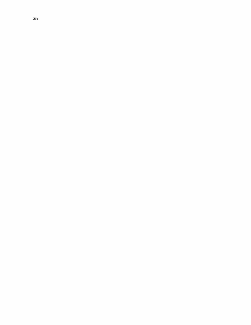
���

Set Two
Exercise �
Let � x�� x�� � � � � xn� � B be an ordered orthonormal basis for Euclidean space V � Let
B� � � x�� x�� x�� � � � � xn� �i�e�� just interchange x� and x� �� Show that B and B� are
oppositely oriented�
Exercise
If V is Euclidean vector space� the �identity tensor� on V is de�ned to be that I � V �Vsuch that for any �x� �y � V
I ��x� �y� � �x � �y�
Suppose that �u�� � � ��un� �v�� � � ��vn are �xed vectors in V such that
I �nXi �
�ui�vi�
a� Prove that n � dimV � �Hence� if dimV � � I is not a dyad ��
b� Prove that if n � dimV then ��u�� � � � � �un� is the basis of V dual to ��v�� � � ��vn��
Solutions
� Let A be one of the two unimodular alternating tensors over V � Let � � Sn� Then
A� x���� � � � � x�n�� � � sgn ��A� x�� � � � � xn�� Hence � x�� � � � � xn� and � x���� � � � � x�n��have the same or opposite orientation according as sgn � � �� or ���
��

���
�� Change notation so as to use our restricted summation convention� Write I � �ui�vi�
Then for any �x� �y � V we have
�x � �y � I��x� �y� � ��ui � �x���vi � �y� � �x �h�ui��vi � �y
�i� ��
Thus
�x �h�y �
��y � �vi
��uii� �� ���
For any �xed �y � V � ��� is true for all �x � V � Thus �y � ��y � �vi��ui � ��� or
�y ���y � �vi
��ui� for any �y � V� ���
a� ��� shows that f�u�� � � � � �ung spans V � Hence� n � dimV �
b� If n � dimV � then ��u�� � � � � �un� is an ordered basis for V � Let ��u�� � � � � �un� be
its dual basis� Choose �xed j� k � f�� � � � � ng and set �x � �uj� �y � �uk in ���
Then
�uj � �uk ���ui � �uj
� ��vi � �uk
�or
�j k � �ij��vi � �uk
�� �vj � �uk�
Thus ��v�� � � � � �vn� is a sequence dual to ��u�� � � � � �un�� Since ��u�� � � � � �un� is a
basis for V � there is exactly one such dual sequence� namely ��u�� � � � � �un�� Hence�vi � �ui�
Exercise
Let V be an n�dimensional Euclidean space� Let A be any nonzero alternating tensor
over V �that is� A � �nV and A �� ��� Let ��b�� � � � ��bn� be an ordered basis for V � with
dual basis ��b�� � � � ��bn�� Let � A��b�� � � � ��bn�� For each i � f�� � � � � ng de�ne
�vi ��
����i��Ahn� �i��b� � � � �� bi � � ��bn
��
Show that �vi � �bi� When n � � express ��b���b���b�� explicitly in terms of ��b���b���b��� using
only the dot and cross products� not A�

���
Exercise �
Suppose L � L�V V ��
a� Show that there are unique mappings S� K � L�V V � such that S is symmetric
�ST � S�K is antisymmetric �KT � �K� and L � S�K� �Hint� then LT � S�K��
b� Suppose dimV � and A is one of the two unimodular alternating tensors over V �
Suppose K � L�V V � is antisymmetric� Show that there is a unique vector
�k � V such that�
K� A ��k� Show that �k � ��Ahi �K and that
�
K� �k �A� �Hint� Takecomponents relative to a positively�oriented ordered orthonormal basis� Use �����
and page D����
Exercise
Let ��b�� � � � ��bn� be a basis for Euclidean vector space V � its dual basis being ��b�� � � � ��bn��Let L � L�V V ��
a� Show that�
L� �biL��bi� � �biL��bi��
b If L is symmetric� show that V has an orthonormal basis x�� � � � � xn with the property
that there are real numbers l�� � � � � ln such that�
L�Pn
v � lv� xv xv� �Hint� Let lv� be
the eigenvalues of L� See page D����
Solutions
��a� We show that �bj � �v i � �ji� and then appeal to the fact that the dual sequence of an
ordered basis is unique� We have
�bj � �v i ��
����i���bj �Ahn� �i��b�� � � � �� bi � � ��bn
��
����
i��
A��bj��b�� � � � ��bi����bi��� � � � ��bn
��

���
It takes i� � interchanges to change ��bj��b�� � � � ��bi����bi��� � � � ��bn� into��b�� � � � ��bi����bj��bi��� � � � ��bn�� and each changes the sign of A� so
�bj � �v i ��
A��b�� � � � ��bi����bj��bi��� � � � ��bn
��
If j �� i� �bj appears twice� so A��b�� � � � ��bi����bj��bi��� � � � ��bn� � � and �bj � �v i � �� If
j � i� then A��b�� � � � ��bi����bi��bi��� � � � ��bn� is � so �bj � �v i � �� QED�
��b� When n � � � A��b���b���b�� � �b� � Ahi��b��b�� � �b� � ��b� ��b��� and�b�
��
Ahi��b ��b�� � �
�b� ��b�
�b�
� � �
Ahi��b��b�� � � �
�b� ��b� � �
�b� ��b�
�b� ��
Ahi��b��b�� � �
�b� ��b��
��a� Uniqueness� If L � S � K with S � ST and KT � �K then LT � S � K so
S � ���L� LT � and K � ���L� LT ��
Existence� de�ne S � ���L � LT � and K � ���L � LT �� Then ST � S�
KT � �K� and L � S �K�
��b� Uniqueness� Suppose�
K� A � �k� Relative to any pooob we have Kij � �ijkkk so
Kij�ijl � �ijl�ijkk
k � �l kkk � kl� Thus� �k �
�
K hiA� Also kl � �lijKij� so
�k � Ahi �K�
Existence� Given�
K antisymmetric� de�ne �k � ��Ahi �
K� We have relative to
any pooob �A � �k
�ij
� �ijkkk �
�
�klmKlm
��
��i
l�jm � �i
m�jl�Klm
��
Kij � �
Kji � Kij�
Hence��
K� A � �k� Also Kij � �ijkkk � kk�kij so
�
K� �k � A�
��a� �bi� �L� L��bi�� Multiply by �bi and sum over i to get �biL��bi� � �bi��b
i� �L� � ��bi�bi�� �L
��
I V ��
L��
L� By viewing �bi as the original and �bi as the dual basis� one then also
�nds �biL��bi� ��
L�

���
��b� From page D��� V has an orthonormal basis x�� � � � � xn consisting of eigenvectors
of L� That is� there are numbers l�� � � � � ln � R such that L� x�� � l� x�� � � � � L� xn� �ln xn� By �a�
�
L�nX
v �
xvL� xv� �nX
v �
xv �lv xv� �nX
v �
lv � xv xv� �
Extra problems
�E� Suppose f�b�� � � � ��bmg is a linearly independent subset of Euclidean space V �so m �dimV � m dimV is possible��� Let ��u�� � � � � �um� and ��v�� � � � � �vm� be any m�tuples
of vectors in V � Show that �ui�bi � �vi�bi implies �ui � �vi�
�E� Suppose V is a Euclidean vector space and a� b� c� d� e are non�negative integers�
Suppose A � �aV � C � �cV � E � �eV � We want to study whether it is true that
Ahbi �ChdiE� � �AhbiC� hdiE� ���
i� Using p �� of the notes� �nd conditions on a� b� c� d� e which imply ����
ii� If dimV � � show that whenever a� b� c� d� e violate the conditions found in i��
it is possible to have A � �aV � C � �cV and E � �lV which violate ����
�Hint� use polyads��
�E� In oriented Euclidean �space �V�A�� show that �u� �v� �w can be chosen so that �u ���v � �w� �� ��u� �v�� �w�
Solutions to Extra Problems
�E� Let U � spf�b�� � � � ��bmg� Then U is a subspace of V and hence a Euclidean vector
space under V �s dot product� Also� ��b�� � � � ��bm� is an ordered basis for U � so in
U it has a dual basis ��b�� � � � ��bm�� If �u i�bi � �v i�bi then ��u i�bi� � �bj � ��v i�bi� � �bj� so�u i��bi ��bj� � �v i��bi ��bj�� so �u i�i
j � �v i�ij� Then �u j � �vj� QED�

���
a
p q
c
q sC r
b
A
s
AE t
d
e
Figure Ex��� Exercise �E�i
�E�i� The picture that makes ��� work is in �gure Ex�� There must be p� q� r� s� t � �
such that a � p � q� b � q� c � q � r � s� d � s� e � s � t� solving for p� q� r� s� t
gives p � a � b� q � b� r � c � b � d� s � d� t � e � d� The conditions that
p� q� r� s� t� a� b� c� d� e � � reduce to
� � b � a� � � d � e� b� d � c�
�E�ii� The question is� is it possible to violate the inequalities in i� in such a way that
Ahbi�ChdiE� and �AhbiC�hdiE are both de�ned� Let hki�P � � order of tensor P �
Thus hki�A� � a� hki�AhbiC� � a � c � b� etc� A product P hqiR is de�ned only
if hki�P � � q and hki�R� � q� If Ahbi�ChdiE� is de�ned we must have a � b�
hki�ChdiE� � c � e� d � b and c � d� e � d� If �AhbiC�hdiE is de�ned we must
have d � e and hki�AhbiC� � d� or a � c � b � d� and also b � a� b � c� If both
triple products are de�ned we must have b � a� b � c� d � c� d � e� b � d � c � e
and b � d � a � c� The only way i� can fail if all these hold is to have b � d � c�
Choose ���� � � � � ��a� ���� � � ���c� ���� � � ���e � V and let A � ��� � � � ��a� C � ��� � � ���c�E � ��� � � ���e� Then we have �gure Ex��ii And AhbiC � ���a�b�� � ���� � � � ���a �

���
a
b
A
C c
E
d
e
Figure Ex�� Figure Ex���ii
��b���� � � � ��a�b��b�� � � ���c �AhbiC�hdiE � ���a�b�� � ���� � � � ���a � ��b����a�c��b�d�� � ����� � � ���a�b � ��d�b�c� ���b�� � ��d�b�c��� � � � ���c � ��d� ��� � � � ��a�c��b�d ��d�� � � ���e�
Similarly ChdiE � ���c�dn � ���� � � � ���c � ��d���� � � ���c�d��d�� � � ���e and Ahbi�ChdiE� �
���a�b�� ����� � � � ���a�b�c�d ���c�d����a�b�c�d�� ���d��� � � � ���a ���b��d�c� ���c�d�� ����� � � � ���c ���d���� � � � ��a�b��b��d�c�� � � ���e�
Choose all ��� ��� �� so the dot products are �� �� Now a � b � a � c � b � d� so
�AhbiC�hdiE � Ahbi�ChdiE� implies that ��a�b and ���d�b�c are linearly dependent�
By choosing them linearly independent we have �AhbiC�hdiE �� Ahbi�ChdiE��
�E�
�u� ��v � �w� � ��u � �w��v � ��u � �v��w��u� �v�� �w � �w � ��v � �u� � ��w � �u��v � ��w � �v��u�
These are equal i� ��u � �v��w � ��v � �w��u� Choose �u and �w mutually � and of unit
length� with �v � �u� �w� and this equation will be violated�

���
Exercise �
Let U be a Euclidean vector space� Let D be an open subset of U � Let�
T� U � U � For
each �u � U � let �f��u� ��
T ��u and g��u� � �u � �u� Show that at every �u � D� �f � D U
and g � D R are di�erentiable� Do so by �nding �r�f��u�� �rg��u�� and the remainder
functions� and by showing that R��h� � as �h ���
Exercise �
Suppose thatDf andDg are open subsets of Euclidean vector spaces U and V respectively�
Suppose that �f � Df Dg and �g � Dg Df are inverse to one another� Suppose there
is a �u � Df where �f is di�erentiable and that �g is di�erentiable at �v � �f��u�� Show that
dimU � dimV � �Hint� See page �����
Exercise ��
Suppose V is a Euclidean vector space� �U�A� is an oriented real three�dimensional Eu�
clidean space� D is an open subset of U � and �f � D U and �g � D V are both
di�erentiable at �u � D�
i� Which proposition in the notes shows that �f�g � D U � V is di�erentiable at �u$
ii� Show that at �u
�r���f�g����r� �f
��g � �f � �r�g�
�Note� In this equation� one of the expressions is unde�ned� De�ne it in the obvious way
and then prove the equation��
Solutions
�a�
�f��u� �h
��
�
T ���u� �h
���
T ��u� �
T ��h

��
� �f��u� � �h� �TT�
Therefore �r�f��u� ��
TTand �R��h� � �� for all �h�
�b�
g��u� �h
��
��u� �h
����u� �h
�� �u � �u� �h � �u� �h � �h� g ��u� � �h � ��u� �
����h��� ����h��� �Therefore �rg��u� � �u� and R��h� �
����h���� As �h �� R��h� � because �h ��
means����h��� ��
�� De�ne�
P� �r�f��u� and�
Q� �r�g��v�� By example ������
P ��
Q��
I U and�
Q � �P��
I V �
Therefore� by ������ the linear mappings P � U V and Q � V U satisfy
Q�P � IU and P �Q � IV � By iii� on page D��� P and Q are bijections� Since they
are linear� they are isomorphisms of U to V and V to U � By preliminary exercise
� dimU � dimV �
���i� Method � on page ��� or method on page ���� applied to �f � � D U �R� and
��g � D R� � V �
���ii� For �u � U and�
P� U � V we de�ne �u� �
P �� Ahi��u�
P
�� Then� relative to any
basis �b�� �b�� �b� for U and ���� � � � � ��n for V � we have ��u� �
P �i l � Aijk�jPkl� Then
h�r�
��f�g�ii
l � Aijkj��f�g�kl� Aijkj �fkgl�
� Aijk ��jfk� gl � fkjgl�
���r� �f
�igl � Aikjfkjgl
�h��r� �f
��gii
l � Aijkfj��r�g
�kl
�h��r� �f
��gii
l ���f � �r�g
�il
�h��r� �f
��g � �f � �r�g
iil� QED�

���
Extra Problems
�E� Let U be a Euclidean vector space� Let�
T� U � U � Let D be the set of all �u � U
such that �u� �T ��u � �� If �u � D� de�ne f��u� � ln��u� �T ��u��
i� Show that D is open�
ii� Show that f � D R is di�erentiable at every point �u � D� and �nd �rf��u��
�E� Let V be the set of all in�nite sequences of real numbers� �x � �x�� x�� � � ��� such thatP n � x
�n converges� If �y � �y�� y�� � � �� is also in V and a� b � R� de�ne a�x � b�y �
�ax� � by�� ax� � by�� � � ��� De�ne �x � �y �P
n � xnyn� �The sum converges by the
Cauchy test because� for anyM and N � Schwarz�s inequality implies jPNn m xnynj �
�PN
n m x�n�����
PNn m y�n�
���� Furthermore� j�x��yj� � j limN� PN
n � xnynj� � limN�
�PN
n � x�n��
Pnn � y
�n� � k�xk�k�yk�� so Schwarz�s inequality works in V �� V is a real
dot�product space but not a Euclidean space� because it is not �nite dimensional�
If �v�� �v�� �v�� � � � is a sequence of vectors in V � de�ne limn� �vn � �v� by the obvious
extension of de�nition ������ i�e� limn� k�v� � �vnk � ��
i� Suppose limn� �vn � �v�� Show that for any �x � V � limn� �x � �vn � �x � �v��
ii� Construct a sequence �v�� �v�� � � � in V such that limn� �x ��vn � � for every �x � V �
but limn� �vn does not exist�
�For di�erentiability� V has two di�erent de�nitions� leading to Frechet and Gateau
derivation respectively based on norms and on components��
Solutions
�E� If�
T���� D is empty and i� and ii� are trivial� Therefore assume k �
T k � �� De�ne
g��u� � �u� �T ��u�

���
i� g��u � �h� � g��u� � �h� �
T ��u � �u� �
T ��h� �
T ��h� Therefore� by the triangle and
generalized Schwarz inequalities�
���g ��u� �h�� g ��u�
��� � k�hkk �
T k�k�uk� k�hk
��
Assume �u � D so g��u� � �� Then �u �� ��� Let � be the smaller of k�uk and
g��u���k�ukk �
T k�� If k�hk � then jg��u � �h� � g��u�j �k �
T k�k�uk � k�hk� �k �
T kk�uk � g��u�� Hence g��u��h�� g��u� � �g��u�� so g��u��h� � �� That
is� if �u � D and � � smaller of �u and g��u���k�ukk �
T k� then the open ball
B��u� �� � D� Hence D is open�
ii� By i� above� g��u � �h� � g��u� � �h � ��T ��
TT� � �u � k�hkR��h� where R��h� �
��h� �T ��h��k�hk for �h �� �� and � �� for �h � ��� Thus g is di�erentiable at �u� with
�rg��u� � ��
T ��
TT���u� By the chain rule� f �g is di�erentiable� with f�v� � lnv�
and its gradient is vf�v��rg��u� where v � g��u�� This is v���rg��u�� so
��rln
��u� �T ��u
����u� �
��
T ��
TT�� �u
�u� �T ��u�
�E� i�
j��x � �vn � �x � �v��j � j�x � ��vn � �v��j � k�xkk�vn � �v�k �
if k�vn � �v�k ��
�E� ii� Let �vn � ��� � � � � �� �� �� � � ��� all � except for a � in the n�th place� If �x � V �
�x ��vn � xn � as n � becauseP
� x�n converges� But if k�vn��vk � for some
�v � V then there is an N so large that if n � N then k�vn � �vk ��� If m� n � N
then k�vm��vnk � k�vm��v��v��vnk � k�vm��vk�k�vn��vk � �� But k�vm��vnk �p�
Exercise ��
A mass distributionm occupies a subset D of ordinary Euclidean �space U � Let n be any
unit vector in U and denote by nR the straight line through U �s origin �� in the direction

���
of n� Let w ��r� be the perpendicular distance of the point �r from the axis nR� so that
the moment of inertia of the mass distribution about that axis is J� n� �RD dm��r� w��r���
De�ne�
T � D U�U by requiring for each �r � D that�
T ��r� � r��
I U ��r�r� Here r� � �r ��rand
�
I U is the identity tensor in U�U � The tensor�
J�RD dm��r�
�
T ��r� is called the inertia
tensor of the mass distribution� and is usually written�
J�RD dm��r��r�
�
I U ��r�r ��
a� Show that�
J is symmetric�
b� Show that J� n� � n� �J � n�
c� Show that to calculate�
J it is necessary to calculate only six particular integrals of
real�valued functions on D with respect to the mass distribution m� �Once these
six functions are calculated� the moment of inertia of the body about any axis is
found from ��b��
Exercise ��
In problem ��� suppose the mass distribution rotates rigidly about the axis nR with
angular velocity �* � * n� so that the mass at position �r has velocity �v��r� � �* � r� The
angular momentum of the mass distribution about �� is de�ned as �L �RD dm��r���r��v��r���
and the kinetic energy of the mass distribution is de�ned asK � ��RD dm��r�v��r��� where
v� means �v � �v� Show the following�
a� �L ��
J ��*
b� K � �� �*� �J ��*
c� �L need not be J� n��*�
Exercise ��
The second moment tensor of the mass distribution in problem �� is de�ned as�
M�RD dm��r��r �r�

���
a� Show that tr�
M�RD dm��r�r��
b� Express�
J in terms of�
M � tr�
M and�
I U �
c� Express�
M in terms of�
J � tr�
J and�
I U � ��
J can be observed by noting the reaction
of the mass distribution to torques� Then �c� gives�
M and �a� givesRD dm��r�r�
from such observations��
d� If the mass distribution is a cube of uniform density �� side a and center at ��� �nd
J� n� when nR is the axis through one of the corners of the cube�
Exercise �
Let y�� y�� y� be an orthonormal basis for physical space P � Let c be a �xed scalar� For
any �r � P � write �r � ri yi� Consider a steady �uid motion whose Eulerian description �vE
is given by
�vE��r� t� � r� y� � c r� y� � �r � � y� y� � c y� y��
for all �r � P and all t � R�
a� Find the Lagrangian description of this motion� using t��position labels�
b� Show that the paths of the individual particles lie in planes r� � constant� and are
hyperbolas if c � �� and straight lines if c � ���
c� Find the label function �x E � P �R P � �It will depend on which �xed t� is used to
establish t��position labels��
d� Find the Eulerian and Lagrangian descriptions of the particle acceleration �a�
Solutions
�� a� The permutation operator ���� P � P P � P is linear� and ����
T ��r� ��
T ��r��
so
���ZDdm��r �
�
T ��r � �ZDdm��r� ���
�
T ��r � �ZDdm��r �
�
T ��r ��
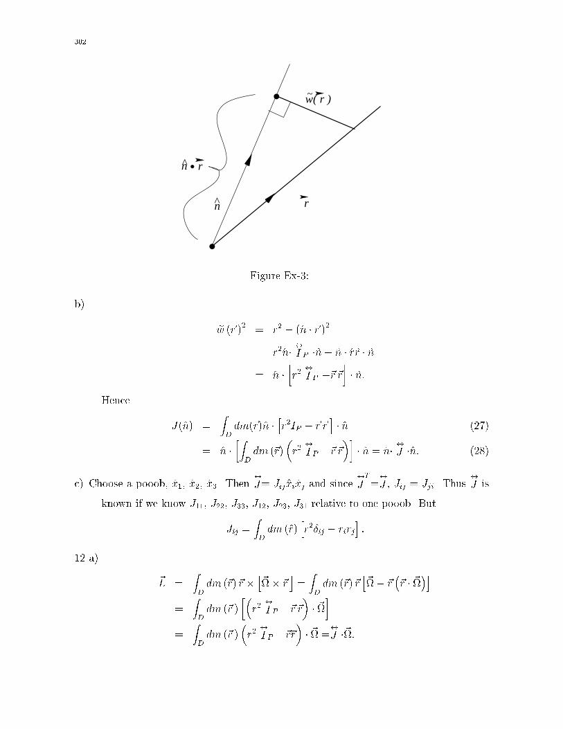
���
rn
.
.
.n r^
w( r )~
Figure Ex��
b�
ew ��r �� � r� � � n � �r ��
� r� n� �I P � n� n � r r � n� n �
�r�
�
I P ��r �r�� n�
Hence
J� n� �ZDdm��r� n �
hr�IP � �r �r
i� n ���
� n ��Z
Ddm ��r�
�r�
�
I P ��r �r��� n � n� �J � n� ���
c� Choose a pooob� x�� x�� x�� Then�
J� Jij xi xj and since�
JT��
J � Jij � Jji� Thus�
J is
known if we know J��� J��� J��� J��� J��� J�� relative to one pooob� But
Jij �ZDdm � r�
hr��ij � rirj
i�
� a�
�L �ZDdm ��r��r �
h�*� �r
i�ZDdm ��r��r
h�*� �r
��r � �*
�i�
ZDdm ��r �
��r�
�
I P ��r �r�� �*�
�ZDdm ��r �
�r�
�
I P ��r�r�� �* �
�
J ��*�

���
b�
K ��
ZDdm ��r �
��*� �r
����*� �r
��
�
ZDdm ��r� * �
h�r �
��*� �r
�i�
�
ZDdm ��r � �* �
hr��*� �r
��r � �*
�i�
�
ZDdm ��r�
��* �
�r�
�
I P ��r �r�� �*�
��
�* �
�ZDdm ��r�
�r�
�
I P ��r�r��� �*
��
�*� �J ��*�
c� Let the mass distribution consist of a single mass point m at position �r� Then
�
J � m�r�
�
I P ��r �r�
�L ��
J ��* � m*�r�
�
I P ��r �r�� n
� m*hr� n� �r ��r � n�
iJ � n� �* �
� n� �J � n
� n* � m*
hr� � � n � �r ��
i n�
If �L � J� n��* then �r�� � n ��r��� n � r� n��r��r � n�� so ��r � n�� n � ��r � n��r� To violate
this condition choose n so it is neither parallel nor perpendicular to �r�
� a� tr � P � P R is linear� so
tr�
M � trZDdm ��r��r �r �
ZDdm ��r� tr�r�r
�ZDdm ��r� r��
b��
J�Rdm��r�
�r�
�
I P ��r �r�� �
RD dm ��r� r��
�
I P � RD dm ��r��r �r
� ����J��
I P
�tr
�
M
�� �
M �
c� From the above equation� since tr � P � P R is linear�
tr�
J��tr
�
I P
��tr
�
M
�� tr
�
M� tr�
M �tr �
M� tr�
M �
Hence� tr�
M� �� tr�
J and�
M� ���
I P �tr�
J �� �
J �
���
d� Let x�� x�� x� be a pooob parallel to the edges of the cube� Then
Mij �Zcube
dx� dx� dx� xixj�
� �Z a
�adx�
Z a
�adx�
Z a
�adx� xi xj�
Thus Mij � � if i �� j and M�� � M�� � M�� � �a��R a�a x
� � �a���� Therefore�
M� �a����
I P and tr�
M� �a�� so from ��� above�
J���a��
�
I P �
Then for any n� n� �J � n � ��a����
�� a�
dr�
dt� r��
dr�
dt� cr��
dr�
dt� � so
r� � A�et�t��� r� � A�ect�t��� r� � A��
The label �x � xi yi belongs to the particle which was at that position at t � t�� For
this particle when t � t�� ri � xi� so xi � Ai� Thus
��� r� � x�et�t��� r� � x�ect�t��� r� � x��
�r � ri yi � et�t��x� y� � ect�t��x� y� � x� y�
� �x �h y� y�e
t�t�� � y� y�ect�t�� � y� y�
i�
�r L ��x� t� � �x �h y� y�e
t�t�� � y� y�ect�t�� � y� y�
i�
b� y� � �r is independent of time for each particle� so each particle lies in a plane y� � �r �
constant� And for a particular particle� r�r� � x�x�e��c�t�t�� � x�x� if c � ���which is a hyperbola� And r��r� � ec���t�t��x��x� � x��x�� if c � ��� Then this
is a straight line through the y� axis�
c� From ��� above� x� � r�e�t�t��� x� � r�e�ct�t��� x� � r�� so
�x � xi yi � r�e�t�t�� y� � r�e�ct�t�� � r� y�
� �r �h y� y�e
�t�t�� � y� y� e�ct�t�� � y� y�
i�
�x E ��r� t� � �r �h y� y� e
�t�t�� � y� y� e�ct�t�� � y� y�
i�

���
d�
�aL ��x� t� � D�t �r
L ��x� t� � �x �h y� y� e
t�t�� � y� y� ect�t��
i�aE ��r� t� � �x E ��r� t� �
h y� y� e
t�t�� � c� y� y� ect�t��
i
�aE ��r� t� � �r �h y� y� e
�t�t�� � y� y� e�ct�t�� � y� y�
i�h y� y� e
t�t�� � c� y� y� ect�t��
i� �r �
h y� y� � c� y� y�
i�
Another way to get the same result is to observe that
�vE ��r� t� � �r � � y� y� � c y� y��
has no explicit t dependence� so t�vE��r� t� � ��� Also ��vE��r� t� � y� y� � c y� y�� so
�vE � ��vE ��r� t� � �r � � y� y� � c� y� y��� But
�aE ��r� t� � Dt�vE ��r� t�
� t�vE ��r� t� � �vE � ��vE ��r� t�
� �� � �r �� y� y� � c� y� y�
��
Exercise �
a� Given a continuum and a function f � R W which depends on t alone �W is a
Euclidean vector space�� invent a physical quantity which can reasonably be called
f � and show that �Dtf�L�t� � �tf�
E�t� � �tf�t��
b� A continuum undergoes rigid body motion� At time t the position� velocity and
acceleration of the pivot particle are �R�t�� �V �t� � �t �R�t� and �A�t� � �t�V �t�� and the
angular velocity relative to the pivot particle is �*�t�� Find the Eulerian description
of particle acceleration in the material�

���
Exercise ��
Several decades ago� before the big bang was accepted� Fred Hoyle suggested that the
expanding universe be explained by the continuous creation of matter� Then mass is not
quite conserved� Suppose that a certain region of space is occupied by a continuum� and
that at position �r at time t new matter is being created at the rate of �E��r� t� kilograms
per cubic meter per second� Make the necessary changes in the derivation of the Eulerian
form of the law of conservation of mass and in equations ������� and ���������
Exercise �
At time t� in a certain material� the Cauchy stress tensor�
S is symmetric�
a� Let K � be an open set in the region occupied by the material� and suppose its boundary
K � is piecewise smooth� Show that the total force �F and the total torque �L about
�� exerted on K � by the stress on K � are the same as those exerted by a �ctitious
body force with density �� �S newtons � m� acting in K ��
b� Write the Taylor series expansion of�
S about �� in physical space P as�
S ��r� ��
S��
��r � S�� � ����r �r�hiS�� � � � � where �
S����
S����
S��� � � � are constant tensors in
P �P � ��P � ��P � � � � and ���S�� � S��� Neglect all terms except those involving�
S����
S��� and
�
S��� and calculate �F and �L of a� for K � � B���� c�� the solid ball of
radius c centered on ���
Hint �� Do all calculations relative to an orthonormal basis in P �
Hint � Use the symmetry of B���� c� to evaluateRB dV ��r�rirj�
Solutions
�� a� The physical quantity has as its Lagrangian description fL��x� t� � f�t�� Then its
Eulerian description is fE��r� t� � f�t�� Since � �f � �� Dtf � tf � �v � � �f � tf �

��
b�
�vE ��r� t� � �V �t� � �*�t��h�r � �R�t�
i� �V �t� �
h�r � �R�t�
i� �* �t��
��vE ��
* so
�vE � ��vE � �vE� �*� �*� �vE � �*� �V � �*�h�*�
��r � �R
�it�v
E � �A�t�� �V �t�� �* �h�r � �R
i� t
�
*
� �A� �*� �V � t�*���r � �R
��
�Dt�v�E � �aE �
�t�v � �v � ��v
�E� �A� t�*�
��r � �R
�� �*�
h�*�
��r � �R
�i�aE ��r� t� � �A�t� �
h�r � �R�t�
i��t
�
* ��
* � �*��
��� The amount of mass in K ��t� is
M �K ��t�� �ZK�t�
dVP ��r��E��r� t��
It is a mathematical identity �derivative over moving volume� that
d
dtM �K ��t�� �
ZK�t�
dVPt�E �
Z�K�t�
dAp np ���vE�E
��
ZK�t�
dVpht� � � � ���v�
iE��r� t� �
Hoyle�s new physical law is that
d
dtM �K ��t�� �
ZK�t�
dVp �E��r� t��
Therefore ZK�t�
dVpht�� � � ���v�� �
iE��r� t� � ��
Since this is true for every open set K ��t� with piecewise smooth boundary� the
vanishing integral theorem gives
t� � � � ���v� � ��

���
Then for any other physical quantity �f �
d
dt
ZK�t�
dVP���f
�E�
ZK�t�
dVPh�t�� �f � �
�t �f
�iE�ZK�t�
dAP n �h�v���f
�iE�
ZK�t�
dVPh�t�� �f � �
�t �f
�� � �
���v �f
�iE�
ZK�t�
dVPn�t�� �f � �
�t �f
��h� � ���v�
i�f � ��v � �f
oE�
ZK�t�
dVPn��t �f � �v � t �f
��ht�� � � ���v�
i�foE
�ZK�t�
dVPh�Dt
�f � � �fiE
�� a�
Z�K�
dA n� �S�ZK�
dV��� �S
��Z
�K�
dA�r �� n� �S
��i� �
�ZK�
dA�n� �
S ��r�i
� �ZK�
dV�� �
��
S ��r��
i� �
ZK�
dV j �Sjkrl�kli�
� ��iklZK�
dV �rljSjk � �jlSjk�
� ��ikjZK�
dV �rjlSlk � �jlSlk�
� �ijk
ZK�
dV �rjlSlk � Sjk�
�ZK�
dV��r � �� �S
�i�
b�
Sij � S��ij � rkS
��kij �
�
rkrlS
��klij
iSij � S��iij �
�
��k ir
l � �l irk�S��klij
� S��iij �
�
�rlS
��ilij � rkS
��kiij
�iSij � S
��iij � rkS
��kiij � vj � rkwkj
� de�nes vj and wkj��

���
�� �S � �v � �r� �w �
�r � �� �S � �r � �v � �r ���r� �w
���r � �� �S
�i
� ��r � �v�i � �ijkrjrlwlkZBdV �� �S � jBj�v �
�ZBdV �r
�� �w�
ZBdV �r �
�� so
�F ���
c��v �
��
c� tr�� S
��
�L �ZBdV �r � �� �S� Li �
ZBdV �ijk �rjvk � rjrlwlk� �
ZBdV rj � � and
RB dV rjrl � ����� c��jl so Li � ����� c��ijkwjk� �L � ����� c�
Ahitr��S�� �
Exercise ��
a� The angular momentum of a single dysprosium atom is ��h��� where h is Planck�s
constant� The density of dysprosium is ����gm�cm�� and its atomic weight is
������ Compute the angular momentum of a stationary ball of solid dysprosium
with radius r cm if all the dysprosium atoms are aligned in the same direction� If
the dysprosium atoms had no angular momentum� how rapidly would the ball have
to rotate as a rigid body in order to have the same angular momentum$
b� Let y�� y�� y� be a positively oriented ordered orthonormal basis for physical space P �
A permanent alnico magnet has magnetization density �M � M y� where M � ���
amp�meter �close to the upper limit for permanent magnets�� The magnet is held at
rest in a uniform magnetic �eld �B � B y� with B � � tesla �about the upper limit for
commercial electromagnets�� Then the volume torque on the magnet is �m � �M � �B
joules �meter�� Suppose that the magnet�s intrinsic angular momentum density �l
does not change with time� and that its torque stress tensor�
M vanishes� Let�
S be
the Cauchy stress tensor in the magnet� Find ����
S � �
ST�� the antisymmetric part
of�
S� in atmospheres of pressure �one atmosphere � ����� ��� newtons�meter� �
�������� dynes �cm� �� If the symmetric part of�
S� ����
S ��
ST�� vanishes� sketch

���
1 meter
1 meter
^
^^
^
^
^
n 5
S
n
5
S
4
4
n3
S3
x
y
z S1
n1
S2
n 2
Figure Ex���
the stresses acting on the surface of a small spherical ball of material in the magnet�
Exercise ��
a� Give the obvious de�nition of the stu� �y component of momentum�� Give its �,� �F ��
its ��� �F �� and its creation rate ��
b Show that in a material at rest with no body forces� the material �ux density �F of y
momentum satis�es � � �F � �� �If �F were the velocity of a �uid� the �uid would be
incompressible��
c� An aluminum casting �� cm thick and � meter on each side is shaped as in �gure Ex���
A steel spring is compressed and placed between the jaws of the casting as shown�
The spring and casting are at rest and gravity is to be neglected� Roughly sketch

���
the �eld lines of �F �the material �ux density of y momentum� in the casting� �If
�F were a force �eld� the �eld lines would be the lines of force� if �F were a velocity
�eld� they would be the streamlines��
Hint for c�� Estimate qualitatively the sign of the y component of the force exerted
by the aluminum just in front of �Si� ni� on the aluminum just behind it for
the surfaces i � �� � � �� � sketched in the �gure�
Note for c�� The x axis points out of the paper� the y axis is parallel to the axis of
the spring� and the z axis points up� as shown in the �gure�
Solutions
�� a� There are ����� ���������� � ��� ���� atoms in a gram of Dysprosium� Each
has angular momentum ������������ � ����� erg sec� If all are aligned� one
gram of Dy has angular momentum l � �� � ���� erg sec�gm� A Dy ball of
radius r cm has intrinsic angular momentum ������r�l� If this angular momentum
were not intrinsic� but due to an angular velocity � of rigid rotation� the angular
momentum would be ����r�������r��� Thus l � ���� r��� or � � ���� l�r� �
��� �����r� radians�sec� with r in cm�
b�
�� � �m� Ahi �S� so relative to the pooob y�� y�� y�
� � mi � �ijkSjk� Then
� � mi�ilm � �ilm�ijkSjk
� � mi�ilm � ��lj�mk � �lk�mj�Sjk � mi�ilm � Slm � Sml�
��� �
�Slm � Sml� � ��
�lmimi�
In our problem� �m � MB y� so
�
�S�� � S��� � ��
MB�
�
�S�� � S��� �
�
�S�� � S��� � �� and
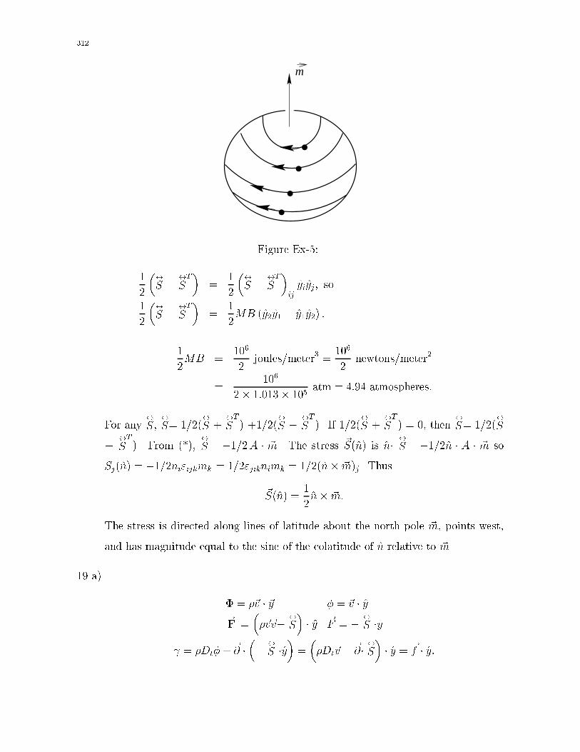
���
....
m
Figure Ex���
�
��
S � �
ST�
��
��
S � �
ST�ij yi yj� so
�
��
S � �
ST�
��
MB � y� y� � y� y�� �
�
MB �
���
joules�meter� �
���
newtons�meter�
����
� ����� ���atm � ���� atmospheres�
For any�
S��
S� ����
S ��
ST� ����
�
S � �
ST�� If ���
�
S ��
ST� � �� then
�
S� ����
S
� �
ST�� From �/��
�
S� ���A � �m� The stress �S� n� is n� �S� ��� n � A � �m so
Sj� n� � ���ni�ijkmk � ���jiknimk � ��� n� �m�j� Thus
�S� n� ��
n� �m�
The stress is directed along lines of latitude about the north pole �m� points west�
and has magnitude equal to the sine of the colatitude of n relative to �m�
�� a�
, � ��v � �y � � �v � y�F �
���v�v� �
S
�� y �F � � �
S � y
� � �Dt�� � ��� �
S � y����Dt�v � �� �S
�� y � �f � y�

���
n4
n5^
^
^
^
^
x
z
y
^
^
n3
n1
n2
Figure Ex���
b� If �f � � and �v � �� then �� �S� �� so ��� �S� � y � � � ��S � y� � ��
c� �F � � �
S � y� The double arrows show ni��
S on the �ve surface sections� Then
on S�� n� � �F � y ��� �
S � y�� � y� �S � y � �
� n��
�
S
�� y � �
on S�� n� � �F � � z ��� �
S � y�� �
�� z� �S
�� y � �
� n��
�
S
�� y � �
on S�� n� � �F � � y ��� �
S � y�� �
�� n��
�
S
�� y � � above
� below
on S�� n� � �F � z ��� �
S � y�� �
� n��
�
S
�� y � �
on S�� n� � �F � y ��� �
S � y�� �
� n��
�
S
�� y � ��
Thus the �ow lines are as in �gure Ex���

���
Figure Ex���
Exercise ��
Geological evidence indicates that over the last � million years� the west side of the San
Andreas fault has moved north relative to the east side at an average rate of about �
cm�year� On a traverse across the fault� Brune� Henyey and Roy ������ �J�G�R� ���
��� found no detectable extra geothermal heat �ow due to the fault� They estimate that
they would have detected any anomalous heat �ow larger than ��� ���� watts�meter��
Use �������� to obtain an upper bound on the northward component of the average stress
exerted by the material just west of the fault on the material just east of the fault� Assume
that the fault extends vertically down from the surface to a depth D� and that the shape
of the heat �ow anomaly due to the fault is a tent function whose width is D on each side
of the fault�

���
D
D D
North Pacific Plate
San Andreas Fault
east
American Plate
up
east
Extra heat flow due to fault, watts /m2
. .Figure Ex���

���
Solutions
�� We assume that the heat �ow is steady� Since we are interested only in averages� we
may assume that ��
S��� is constant on the fault� as is � � � �H���� D is probably � km
�see Brune et al� ����� so we may treat the fault as in�nitely long� Then �H lies in
east�west vertical planes� Consider a length L along the fault� The amount of heat
produced by this section of the fault in LD� � � �H���� It all �ows out of the surface of
the earth in a rectangle of length L along the fault and width D across the fault� the
pro�le being the triangular one sketched as the bottom �gure in the exercise� The
area under that triangle is Dh where h is the triangle�s height� so the total heat �ow
out in the length L and width D is LDh� This must equal LD� � � H��� in the steady
state� Thus h � � � � H���� Since no anomaly was detected� h � �� � ����w�m��
Thus � � � H��� � � � ��S��� � ��v��� � ��� ����w�m�� Let x be a unit vector pointing
north� and let y � � point west� Then ��v��� � � x cm�yr � � � ���� x meters�yr
� � ���� x meters�sec� The heat production must be positive� so
� � � ���
S
���� x�� ����
�� ��� �����
or
� �� �� �S
���� x � ��� ��� pascals�
The material just west of the fault exerts on the material just east of the fault� a
stress � �� �S���� The northward component of this stress is � �� �S��� � x� and it lies
between � and �� bars ���� pascal ��
See Brune et al�� for a discussion of energy loss from �v � ��S��� � ��v��� by seismic
radiation� This exercise works only for the parts of the fault where most energy is
not radiated� i�e�� the parts of the fault which creep�
Exercise ��
Below are the Eulerian descriptions of three motions of continua� In these descriptions�
f x� y� zg is a right�handed orthonormal basis for physical space P � � is a constnat real

��
number� and �* is a constant vector� For each motion� �nd the local strain rate tensor��� �
its eigenvectors� and its eigenvalues� Also �nd the local rotation rate tensor���� and the
local angular velocity�
�w�
a� �vE��r� t� � ��r � � x x� y y� � ��x x� y y�
b� �vE��r� t� � ��r � � y x� � �y x
c� �vE��r� t� � �*� �r �
Exercise ��
Let �v�#�� �
#�� be the Eulerian descriptions of the velocity� local strain rate tensor and local
rotation rate tensor in a certain continuum� Let x�� x� x� be a right�handed orthonormal
basis in physical space P � Let position vectors be written �r � ri xi� Let i denote the
partial derivative with respect to ri� Take tensor components relative to x�� x�� x��
a� Show that i��jk� j
��ki �k �
�ij
b� Show that ij��kl �jk �
�li �kl��ij �li �
�jk� ��
c� Show that if��� � P P � P is any tensor�valued function of �r such that everywhere
��ij�
��ji and b� holds� then a function
���� P P � P can be found which satis�es
��ij� � �
�ji and also a� above� Show that this function is unique up to an additive
constant tensor
��
* which is antisymmetric�
d� Show that if��� is the function in c�� there is a velocity function �v � P P whose local
strain rate tensor is��� � Show that any two such functions �v� and �v� di�er by the
velocity �eld of a rigid motion� that is� there are �xed vectors �* and �V such that
for all �r � P � �v���r�� �v���r� � �V � �*� �r�
Hint for c� and d�� Suppose gi � P R for i � �� � � You know from elementary
vector calculus that there is a �potential function� f � P R such that gi � if i�
igj � jgi everywhere� and if this is so� then f��r� � f���� �R �r� drigi �line integral��

���
Exercise ��
Use the notation beginning on page �� for discussing small disturbances of an HTES of
an elastic material whose reference state is HTES��
a� Using only ����
S�� B���
W �� ���
��
Q�� explicitly express U � U� as a function of �N and
��
G� correct to second order �i�e�� including the terms ��N��� �N��
G and ��
G ��
G��
b� The tensor
��
F �� is called the isentropic or adiabatic sti�ness tensor because if �N � �
�no change in entropy� then
��
S� ��
G hi��
F �
Find the isothermal sti�ness tensor
��
F ��� the tensor such that if �� � � then
��
S� ��
G hi��
F �� �
Express
��
F �� in terms of
��
F ���
W � B�� ���
Exercise �
Using the notation on page ��� give the results of a�� b� when HTES� is isotropic�
Solutions
� a�
��vE � � � x x� y y� ����vE
�T�
so���� � � x x� y y� �
eigenvectors and eigenvalues being � x� ��� � y����� � z���������
��� so
�
��� ���

���
b�
��vE � � y x����vE
�T� � x y�
��� �
�
� x y � y x� �
����
�
� y x� x y�
eigenvectors and eigenvalues of��� are�
x� yp��
��
� x � yp
���
�� � z� �� �
�
�w��
Ahi
����
�
�
� y � x� x� y� � ��
� z
c� Let�
*� A � �*� Then
�vE � Ahi�*�r � ��* � A � �r� � �
* ��r � �r� �* �
Then ��vE ��
*����vE
�T� � �
*� so����
�� �so all eigenvalues are � and any vector is
an eigenvector�����
�
*��
��� �*�
� a�
#�jk ��
�jvk � kvj�
#�ij ��
�ivj � jvi�
k #�ij ��
�kivj � kjvi�
Replace �ijk� by �kij� and this becomes
j #�ki ��
�jkvi � jivk� �
i #�jk ��
�ijvk � ikvj� �
Comparing these three equations gives a��

���
b� il #�jk � li #�jk so� by a��
i �j #�kl � k #�lj� � l �j #�ki � k #�ij�
or� since #�kl � #�lk and ij � ji�
ji #�kl � ik #�lj � ki #�li � lj #�ik � ��
Now make the replacements j i� i j� and one proves b��
c� Fix i and j� a� can be written
��� k #�ij � i #�jk � j #�ki�
Then b� implies kl #�ij � lk #�ij� which are exactly the integrability conditions for
�/�� They insure that the line integralZ �r
��drk �i #�jk � j #�ki�
will be independent of path� Thus the solution of �/� exists� and has the form
#�ij��r� � � #�ij���� �Z �r
��drk �i #�jk � j #�ik� �
The integral is antisymetric in ij� If #�ij���� is chosen antisymmetric in ij� #�ij��r�
will be antisymmetric for all �r�
d� Let #�ij��r� be given as in c�� We want to try to solve
ivj � #�ij � #�ij�
This will be possible� and the solution will be
vj��r� � Vj �Z �r
��dri � #�ij � #�ij� �
as long as for each �xed j the integrability condition kivj � ikvj is satis�ed�
i�e��
�y� k � #�ij � #�ij� � i � #�kj � #�kj� �
But #�ij was obtained by solving �/� on the preceding page� Substituting �/� in �y�makes �y� an identity�

���
� a�
U � U� � �NNU � ��
G hi��GU
��
��N�� �NU � �N�
G hi��GNU
��
���
G ��
G
�h�i��
G��GU � third order terms
� �N�� � ��
G hi�
S�
���
�
��N��B�
��N��
G hi�
W�
���
�
���
G ��
G
�h�i
��
Q�
��� third order term�
b�
�� � �NB� � ��
G hi�
W �
��
��
S � �N�
W � ���
G hi��
F � �
If �� � �� then �N � �� �
G hi�
W�
��B�� so
��
S� ��
G hi�� ��
F � ��
W �
�
W �
��B�
A �
Therefore��
F ���
��
F� ��
W �
�
W �
��B��
�� In an isotropic material�
�
S� � �p��
I�
W � � �� �
I
Fijkl � �ij�kl � � ��ik�jl � �il�kj�
Qijkl � Fijkl � �ijS��kl � �jkS
��il
� Fijkl � p� ��jk�il � �ij�kl�
Qijkl � �� p�� �ij�kl � � �ik�jl � ��� p�� �jk�il

���
a�
U � U� � �N�� � p���
�tr �
�
G
��
�
��N��B�
� �
����N�
�tr �
�
G
��
�
��
n�� p��
�tr �
�
G
��� � �
�
G hi� �
G
���� p�� ��
G hi� �
GTo
� third order terms�
b�
��ij�kl � �� ��ik�jl � �il�jk�
� �ij�kl � � ��ik�jl � �il�jk�� ��
��B��ij�kl�
Thus �� � �� � � � �����B��