A Continuum Mechanics Premier

8/9/2019 A Continuum Mechanics Premier

http://slidepdf.com/reader/full/a-continuum-mechanics-premier 1/99

A CONTINUUM MECHANICS PRIMER

On Constitutive Theories of Materials

I-SHIH LIU

Rio de Janeiro





Preface

In this note, we concern only fundamental concepts of continuum mechanics for theformulation of basic equations of material bodies. Particular emphases are placed ongeneral physical requirements, which have to be satisfied by constitutive equations of material models.

After introduction of kinematics for finite deformations and balance laws, constitu-tive relations for material bodies are discussed. Two general physical requirements forconstitutive functions, namely, the principle of material frame-indifference and the ma-terial symmetry, are introduced and their general consequences analyzed. In particular,concepts of change of frame, Euclidean objectivity and observer-independence of mate-rial properties are carefully defined so as to make the essential ideas of the principle of material frame-indifference clear.

Constitutive equations and governing equations for some special classes of mate-rials are then derived. For fluids, these includes elastic fluids, Navier-Stokes fluids,Reiner-Rivlin fluids, viscous heat-conducting fluids and incompressible fluids. For solids,

are discussed isotropic elastic solids, anisotropic elastic solids, neo-Hookean material,Mooney-Rivlin materials for finite deformations in general as well as linearizations forsmall deformations, the Hookes’ law in linear elasticity and the basic equations of linearthermoelasticity.

The constitutive theories of materials cannot be complete without some thermody-namic considerations, which like the conditions of material objectivity and material sym-metry are equally important. Exploitation of the entropy principle based on the generalentropy inequality and the stability of equilibrium are considered. The use of Lagrangemultipliers in the evaluation of thermodynamic restrictions on the constitutive functionsis introduced and its consequences for isotropic elastic solids are carefully analyzed.

This note can be regarded as a simplified and revised version of the book by the

author (Continuum Mechanics , Springer 2002). It has been used in a short course formathematics, physics and engineering students interested in acquiring a better knowledgeof material modelling in continuum mechanics.

I-Shih LiuRio de Janeiro, 2006





Contents

1 Kinematics 1

1.1 Configuration and deformation . . . . . . . . . . . . . . . . . . . . . . . . 2

1.2 Strain and rotation . . . . . . . . . . . . . . . . . . . . . . . . . . . . . . 4

1.3 Linear strain tensors . . . . . . . . . . . . . . . . . . . . . . . . . . . . . 51.4 Motions . . . . . . . . . . . . . . . . . . . . . . . . . . . . . . . . . . . . 7

1.5 Rate of deformation . . . . . . . . . . . . . . . . . . . . . . . . . . . . . . 9

2 Balance Laws 13

2.1 General balance equation . . . . . . . . . . . . . . . . . . . . . . . . . . . 13

2.2 Local balance equation and jump condition . . . . . . . . . . . . . . . . . 15

2.3 Balance equations in reference coordinates . . . . . . . . . . . . . . . . . 16

2.4 Conservation of mass . . . . . . . . . . . . . . . . . . . . . . . . . . . . . 17

2.5 Equation of motion . . . . . . . . . . . . . . . . . . . . . . . . . . . . . . 18

2.6 Conservation of energy . . . . . . . . . . . . . . . . . . . . . . . . . . . . 192.7 Basic Equations in Material Coordinates . . . . . . . . . . . . . . . . . . 21

2.8 Boundary conditions of a material body . . . . . . . . . . . . . . . . . . 21

3 Constitutive Relations 23

3.1 Frame of reference, observer . . . . . . . . . . . . . . . . . . . . . . . . . 23

3.2 Change of frame and objective tensors . . . . . . . . . . . . . . . . . . . 25

3.3 Constitutive relations . . . . . . . . . . . . . . . . . . . . . . . . . . . . . 31

3.4 Euclidean objectivity . . . . . . . . . . . . . . . . . . . . . . . . . . . . . 32

3.5 Principle of material frame indifference . . . . . . . . . . . . . . . . . . . 33

3.6 Simple material bodies . . . . . . . . . . . . . . . . . . . . . . . . . . . . 36

3.7 Material symmetry . . . . . . . . . . . . . . . . . . . . . . . . . . . . . . 37

3.8 Some representation theorems . . . . . . . . . . . . . . . . . . . . . . . . 40

4 Constitutive Equations of Fluids 43

4.1 Materials of grade n . . . . . . . . . . . . . . . . . . . . . . . . . . . . . 43

4.2 Isotropic functions . . . . . . . . . . . . . . . . . . . . . . . . . . . . . . 44

4.3 Viscous fluids . . . . . . . . . . . . . . . . . . . . . . . . . . . . . . . . . 48

4.4 Viscous heat-conducting fluids . . . . . . . . . . . . . . . . . . . . . . . . 51

4.5 Incompressibility . . . . . . . . . . . . . . . . . . . . . . . . . . . . . . . 524.6 Viscometric flows . . . . . . . . . . . . . . . . . . . . . . . . . . . . . . . 53



iv CONTENTS

5 Constitutive Equations of Solids 57

5.1 Elastic materials . . . . . . . . . . . . . . . . . . . . . . . . . . . . . . . 57

5.2 Linear elasticity . . . . . . . . . . . . . . . . . . . . . . . . . . . . . . . . 585.3 Isotropic elastic solids . . . . . . . . . . . . . . . . . . . . . . . . . . . . 605.4 Incompressible elastic solids . . . . . . . . . . . . . . . . . . . . . . . . . 615.5 Thermoelastic materials . . . . . . . . . . . . . . . . . . . . . . . . . . . 635.6 Linear thermoelasticity . . . . . . . . . . . . . . . . . . . . . . . . . . . . 645.7 Mooney-Rivlin thermoelastic materials . . . . . . . . . . . . . . . . . . . 665.8 Rigid heat conductors . . . . . . . . . . . . . . . . . . . . . . . . . . . . 70

6 Thermodynamic Considerations 73

6.1 Second law of thermodynamics . . . . . . . . . . . . . . . . . . . . . . . 736.2 Entropy principle . . . . . . . . . . . . . . . . . . . . . . . . . . . . . . . 74

6.3 Thermodynamics of elastic materials . . . . . . . . . . . . . . . . . . . . 756.4 Elastic materials of Fourier type . . . . . . . . . . . . . . . . . . . . . . . 796.5 Isotropic elastic materials . . . . . . . . . . . . . . . . . . . . . . . . . . 816.6 Thermodynamic stability . . . . . . . . . . . . . . . . . . . . . . . . . . . 83

Bibliography 89

Index 91



CHAPTER 1

Kinematics

Notations

The reader is assumed to have a reasonable knowledge of the basic notions of vector spacesand calculus on Euclidean spaces. Some notations used in this note are introduced here.

A concise treatment of tensor analysis as a preliminary mathematical background forcontinuum mechanics can be found in the appendix of [14].

Let V be a finite dimensional vector space with an inner product, and L(V ) be thespace of linear transformations on V . The elements of L(V ) are also called (second order)tensors. For u, v ∈ V their inner product is denoted by u · v, and their tensor product ,denoted by u⊗ v, is defined as a tensor so that for any w ∈ V ,

(u⊗ v)w = (v ·w)u.

Let {ei, i = 1, · · · , n} be a basis of V , then {ei ⊗ e j , i, j = 1, · · · , n} is a basis for L(V ),and for any T

∈ L(V ), the component form can be expressed as

T = T ijei ⊗ e j =ni=1

n j=1

T ijei ⊗ e j.

Hereafter, we shall always use the summation convention for any pair of repeated in-dices, as shown in the above example, for convenience and clarity. Moreover, althoughsometimes the super- and sub-indices are deliberately used to indicate the contravariantand the covariant components respectively (and sum over a pair of repeated super- andsub-indices only), in most theoretical discussions, expressions in Cartesian componentssuffice, for which no distinction of super- and sub-indices is necessary.

The inner product of two tensors A and B is defined as

A · B = tr ABT ,

where the trace and the transpose of a tensor are involved. In particular in terms of Cartesian components, the norm |A| is given by

|A|2 = A · A = AijAij,

which is the sum of square of all the elements of A by the summation convention.The Kronecker delta and the permutation symbol are two frequently used notations,

they are defined as

δ ij = 0, if i = j ,1, if i = j ,



2 1. KINEMATICS

and

εijk

= 1, if {i,j,k} is an even permutation of {1,2,3},

−1, if

{i,j,k

} is an odd permutation of

{1,2,3

},

0, if otherwise.

One can easily check the following identity:

εijkεimn = δ jmδ kn − δ jnδ km.

Let E be a three-dimensional Euclidean space and the vector space V be its translation

space . For any two points x, y ∈ E there is a unique vector v ∈ V associated with theirdifference,

v = y − x, or y = x + v.

We may think of v as the geometric vector that starts at the point x and ends at thepoint y. The distance between x and y is then given by

d(x,y) = |x− y| = |v|.

Let D be an open region in E and W be any vector space or an Euclidean space.A function f : D → W is said to be differentiable at x ∈ D if there exists a lineartransformation ∇f (x) : V → W , such that for any v ∈ V ,

f (x + v) − f (x) = ∇f (x)[v] + o(v),

where o(v) denotes the higher order terms in v such that

lim|v|→0

o(v)

|v| = 0.

We call ∇f the gradient of f with respect to x, and will also denote it by ∇xxxf , or morefrequently by either grad f or Grad f .

1.1 Configuration and deformation

A body B can be identified mathematically with a region in a three-dimensional Euclideanspace E . Such an identification is called a configuration of the body, in other words, aone-to-one mapping from B into E is called a configuration of B.

It is more convenient to single out a particular configuration of B, say κ, as a reference,

κ : B → E , κ( p) = X . (1.1)

We call κ a reference configuration of B. The coordinates of X , (X α, α = 1, 2, 3) arecalled the referential coordinates , or sometimes called the material coordinates since thepoint X in the reference configuration κ is often identified with the material point p of

the body when κ is given and fixed. The body B in the configuration κ will be denotedby Bκ.



1. CONFIGURATION AND DEFORMATION 3

p

X

x

κ χ

χκ

B

BχBκ

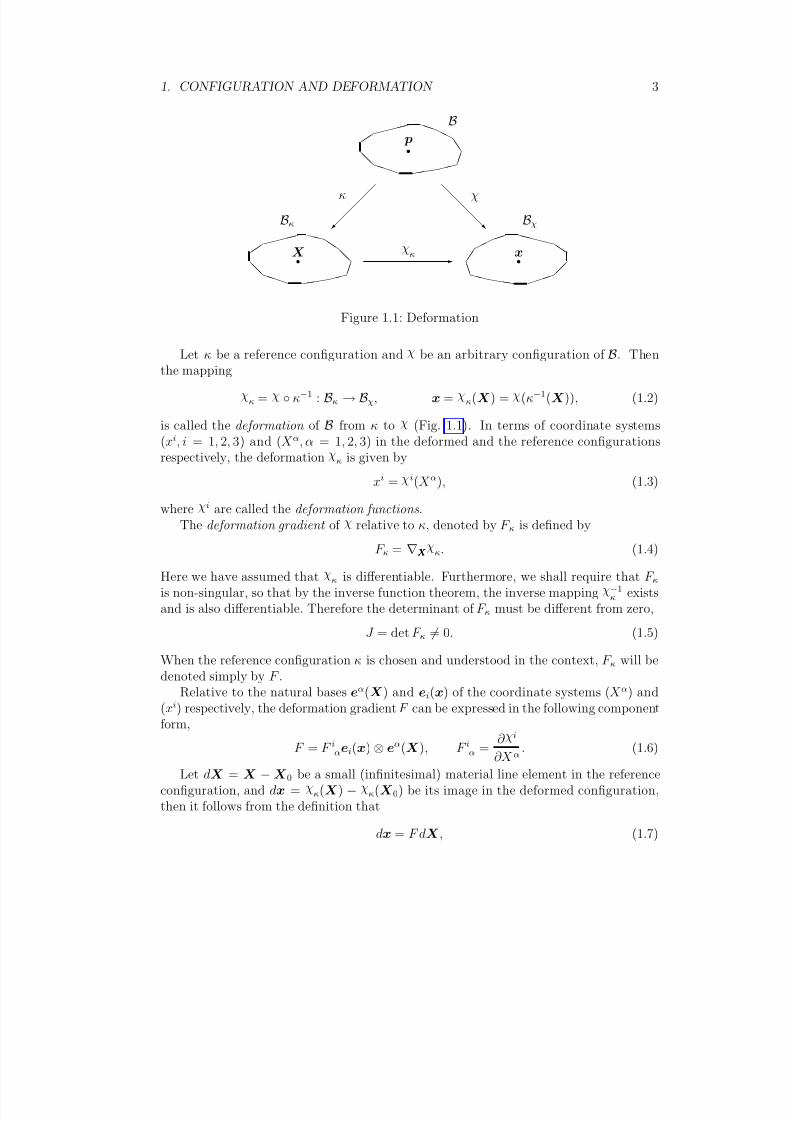
Figure 1.1: Deformation

Let κ be a reference configuration and χ be an arbitrary configuration of B. Thenthe mapping

χκ = χ ◦ κ−1 : Bκ → Bχ, x = χ

κ(X ) = χ(κ−1(X )), (1.2)

is called the deformation of B from κ to χ (Fig. 1.1). In terms of coordinate systems(xi, i = 1, 2, 3) and (X α, α = 1, 2, 3) in the deformed and the reference configurationsrespectively, the deformation χ

κ is given by

xi = χi(X α), (1.3)

where χi are called the deformation functions .The deformation gradient of χ relative to κ, denoted by F κ is defined by

F κ = ∇XX X χκ. (1.4)

Here we have assumed that χκ is differentiable. Furthermore, we shall require that F κ

is non-singular, so that by the inverse function theorem, the inverse mapping χ−1κ exists

and is also differentiable. Therefore the determinant of F κ must be different from zero,

J = det F κ = 0. (1.5)

When the reference configuration κ is chosen and understood in the context, F κ will bedenoted simply by F .

Relative to the natural bases eα(X ) and ei(x) of the coordinate systems (X α) and(xi) respectively, the deformation gradient F can be expressed in the following componentform,

F = F iαei(x) ⊗ eα(X ), F iα = ∂ χi

∂X α. (1.6)

Let dX = X −X 0 be a small (infinitesimal) material line element in the referenceconfiguration, and dx = χ

κ(X ) − χκ(X 0) be its image in the deformed configuration,

then it follows from the definition that

dx = F dX , (1.7)



4 1. KINEMATICS

since dX is infinitesimal the higher order term o(dX ) tends to zero.

Similarly, let daκ and nκ be a small material surface element and its unit normal

in the reference configuration and da and n be the corresponding ones in the deformedconfiguration. And let dvκ and dv be small material volume elements in the referenceand the deformed configurations respectively. Then we have

n da = J F −T nκdaκ, dv = |J | dvκ. (1.8)

1.2 Strain and rotation

The deformation gradient is a measure of local deformation of the body. We shall in-troduce other measures of deformation which have more suggestive physical meanings,such as change of shape and orientation. First we shall recall the following theorem fromlinear algebra:

Theorem (polar decomposition). For any non-singular tensor F , there exist unique symmetric positive definite tensors V and U and a unique orthogonal tensor R such that

F = R U = VR. (1.9)

Since the deformation gradient F is non-singular, the above decomposition holds.We observe that a positive definite symmetric tensor represents a state of pure stretchesalong three mutually orthogonal axes and an orthogonal tensor a rotation. Therefore,(1.9) assures that any local deformation is a combination of a pure stretch and a rotation.

We call R the rotation tensor , while U and V are called the right and the left stretch

tensors respectively. Both stretch tensors measure the local strain, a change of shape,while the tensor R describes the local rotation, a change of orientation, experienced bymaterial elements of the body.

Clearly we have

U 2 = F T F, V 2 = F F T ,

det U = det V = | det F |.(1.10)

Since V = RURT , V and U have the same eigenvalues and their eigenvectors differonly by the rotation R. Their eigenvalues are called the principal stretches, and thecorresponding eigenvectors are called the principal directions .

We shall also introduce the right and the left Cauchy-Green strain tensors defined by

C = F T F, B = F F T , (1.11)

respectively, which are easier to be calculated than the strain measures U and V from a

given F in practice. Note that C and U share the same eigenvectors, while the eigenvaluesof U are the positive square root of those of C ; the same is true for B and V .



3. LINEAR STRAIN TENSORS 5

1.3 Linear strain tensors

The strain tensors introduced in the previous section are valid for finite deformations ingeneral. In the classical linear theory, only small deformations are considered.

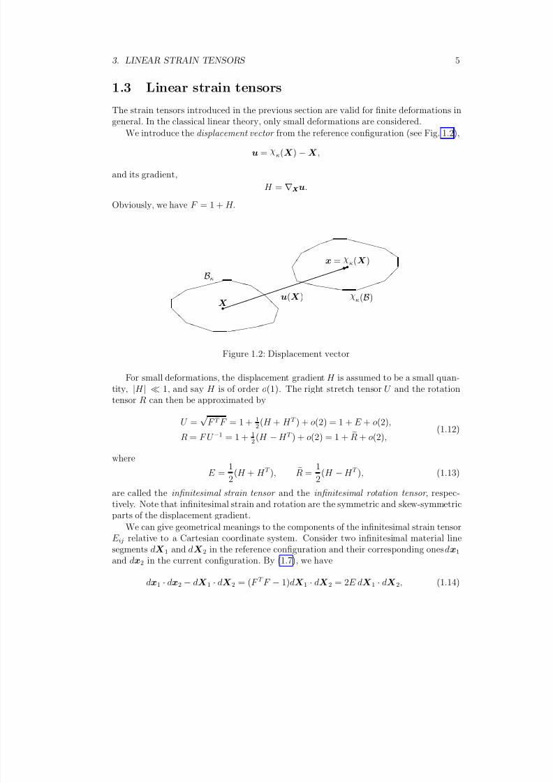
We introduce the displacement vector from the reference configuration (see Fig. 1.2),

u = χκ(X ) −X ,

and its gradient,

H = ∇XX X u.

Obviously, we have F = 1 + H.

X

x = χκ(X )

u(X ) χκ(B)

Bκ

Figure 1.2: Displacement vector

For small deformations, the displacement gradient H is assumed to be a small quan-tity, |H | 1, and say H is of order o(1). The right stretch tensor U and the rotationtensor R can then be approximated by

U =√

F T F = 1 + 12

(H + H T ) + o(2) = 1 + E + o(2),

R = F U −1 = 1 + 12

(H − H T ) + o(2) = 1 +

R + o(2),

(1.12)

whereE =

1

2(H + H T ), R =

1

2(H − H T ), (1.13)

are called the infinitesimal strain tensor and the infinitesimal rotation tensor , respec-tively. Note that infinitesimal strain and rotation are the symmetric and skew-symmetricparts of the displacement gradient.

We can give geometrical meanings to the components of the infinitesimal strain tensorE ij relative to a Cartesian coordinate system. Consider two infinitesimal material linesegments dX 1 and dX 2 in the reference configuration and their corresponding ones dx1

and dx2 in the current configuration. By (1.7), we have

dx1 · dx2 − dX 1 · dX 2 = (F T F − 1)dX 1 · dX 2 = 2E dX 1 · dX 2, (1.14)



6 1. KINEMATICS

for small deformations. Now let dX 1 = dX 2 = soe1 be a small material line segment inthe direction of the unit base vector e1 and s be the deformed length. Then we have

s2 − s2o = 2s2o (E e1 · e1) = 2s2o E 11,

which implies that

E 11 = s2 − s2o

2s2o=

(s − so)(s + so)

2s2o s − so

so.

In other words, E 11 is the change of length per unit original length of a small linesegment in the e1-direction. The other diagonal components, E 22 and E 33 have similarinterpretations as elongation per unit original length in their respective directions.

Similarly, let dX 1 = soe1 and dX 2 = soe2 and denote the angle between the two line

segments after deformation by θ. Then we have

s2o |F e1| |F e2| cos θ − s2o cos π

2 = 2s2o (E e1 · e2),

from which, if we write γ = π/2 − θ, the change from its original right angle, then

sin γ

2 =

E 12|F e1| |F e2| .

Since |E 12| 1 and |F ei| 1, it follows that sin γ γ and we conclude that

E 12

γ

2.

Therefore, the component E 12 is equal to one-half the change of angle between the twoline segments originally along the e1- and e2-directions. Other off-diagonal components,E 23 and E 13 have similar interpretations as change of angle indicated by their numericalsubscripts.

Moreover, since det F = det(1 + H ) 1 + tr H for small deformations, by (1.8)2 fora small material volume we have

tr E = tr H dv − dvκdvκ

.

Thus the sum E 11 + E 22 + E 33 measures the infinitesimal change of volume per unitoriginal volume. Therefore, in the linear theory, if the deformation is incompressible,since tr E = Divu, it follows that

Divu = 0. (1.15)

In terms of Cartesian coordinates, the displacement gradient

∂ui

∂X j=

∂ui

∂xk

∂xk

∂X j=

∂ui

∂xk

(δ jk + o(1)) = ∂ui

∂x j+ o(2),

in other words, the two displacement gradients

∂ui

∂X jand ∂ui

∂x j



4. MOTIONS 7

differ in second order terms only. Therefore, since in the classical linear theory, thehigher order terms are insignificant, it is usually not necessary to introduce the reference

configuration in the linear theory. The classical infinitesimal strain and rotation, in theCartesian coordinate system, are defined as

E ij = 1

2(

∂ui

∂x j+

∂u j∂xi

), Rij = 1

2(

∂ui

∂x j− ∂u j

∂xi

), (1.16)

in the current configuration.

1.4 Motions

A motion of the body B

can be regarded as a continuous sequence of deformations intime, i.e., a motion χ of B is regarded as a map,

χ : Bκ × IR → E , x = χ(X , t). (1.17)

We denote the configuration of B at time t in the motion χ by Bt.In practice, the reference configuration κ is often chosen as the configuration in the

motion at some instant t0, κ = χ(·, t0), say for example, t0 = 0, so that X = χ(X , 0).But such a choice is not necessary in general. The reference configuration κ can be chosenindependently of any motion.

For a fixed material point X ,

χ(X , · ) : IR → E

is a curve called the path of the material point X . The velocity v and the acceleration a

are defined as the first and the second time derivatives of position as X moves along itspath,

v = ∂ χ(X , t)

∂t , a =

∂ 2χ(X , t)

∂t2 . (1.18)

The velocity and the acceleration are vector quantities. Here of course, we have assumedthat χ(X , t) is twice differentiable with respect to t. However, from now on, we shallassume that all functions are smooth enough for the conditions needed in the context,

without their smoothness explicitly specified.A material body is endowed with some physical properties whose values may change

along with the deformation of the body in a motion. A quantity defined on a motioncan be described in essentially two different ways: either by the evolution of its valuealong the path of a material point or by the change of its value at a fixed location inthe deformed body. The former is called the material (or a referential description if areference configuration is used) and the later a spatial description. We shall make themmore precise below.

For a given motion χ and a fixed reference configuration κ, consider a quantity, withits value in some space W , defined on the motion of B by a function

f : B × IR → W. (1.19)



8 1. KINEMATICS

Then it can be defined on the reference configuration,

f : B

κ

×IR

→ W, (1.20)

by f (X , t) = f (κ−1(X ), t) = f ( p, t), X ∈ Bκ,

and also defined on the position occupied by the body at time t,

f (·, t) : Bt → W, (1.21)

by f (x, t) = f (χ−1(x, t), t) = f (X , t), x ∈ Bt.As a custom in continuum mechanics, one usually denotes these functions f , f , andf by the same symbol since they have the same value at the corresponding point, and

write, by an abuse of notations,

f = f ( p, t) = f (X , t) = f (x, t),

and called them respectively the material description , the referential description and thespatial description of the function f . Sometimes the referential description is referred toas the Lagrangian description and the spatial description as the Eulerian description .

When a reference configuration is chosen and fixed, one can usually identify the ma-terial point p with its reference position X . In fact, the material description in ( p, t)is rarely used and the referential description in (X , t) is often regarded as the material

description instead. However, in later discussions concerning material frame-indifferenceof constitutive equations, we shall emphasize the difference between the material descrip-tion and a referential description, because the true nature of material properties shouldnot depend on the choice of a reference configuration.

Possible confusions may arise in such an abuse of notations, especially when differ-entiations are involved. To avoid such confusions, one may use different notations fordifferentiation in these situations.

In the referential description, the time derivative is denoted by a dot while the dif-ferential operators such as gradient, divergence and curl are denoted by Grad, Div andCurl respectively, beginning with capital letters:

f = ∂f (X , t)

∂t , Grad f = ∇XX X f (X , t), etc.

In the spatial description, the time derivative is the usual ∂ t and the differential operatorsbeginning with lower-case letters, grad, div and curl:

∂f

∂t =

∂f (x, t)

∂t , grad f = ∇xxxf (x, t), etc.

The relations between these notations can easily be obtained. Indeed, let f be a scalarfield and u be a vector field. We have

f = ∂f ∂t

+ (grad f ) · v, u = ∂ u∂t

+ (gradu)v, (1.22)



5. RATE OF DEFORMATION 9

andGrad f = F T grad f, Gradu = (gradu)F. (1.23)

In particular, taking the velocity v for u, it follows that

grad v = F F −1, (1.24)

since Grad v = Grad x = F .We call f the material time derivative of f , which is the time derivative of f following

the path of the material point. Therefore, by the definition (1.18), we can write thevelocity v and the acceleration a as

v = x, a = x,

and hence by (1.22)2,

a = v = ∂ v∂t

+ (gradv)v. (1.25)

1.5 Rate of deformation

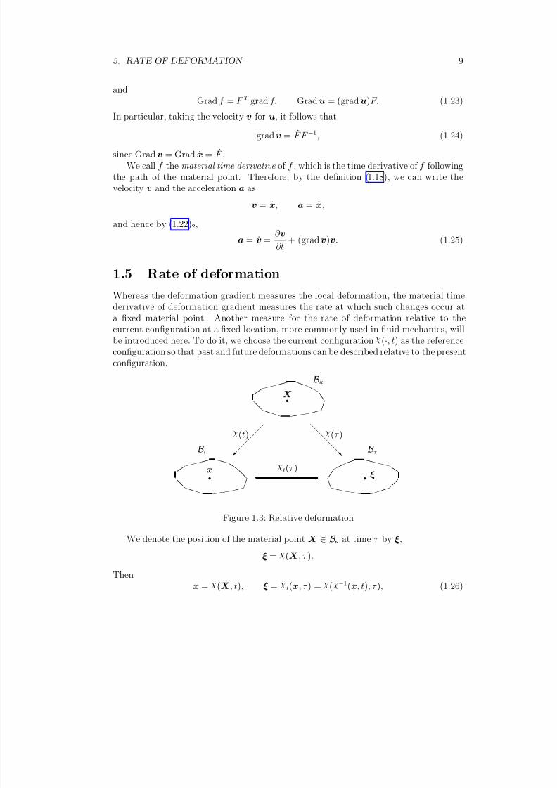
Whereas the deformation gradient measures the local deformation, the material timederivative of deformation gradient measures the rate at which such changes occur ata fixed material point. Another measure for the rate of deformation relative to thecurrent configuration at a fixed location, more commonly used in fluid mechanics, willbe introduced here. To do it, we choose the current configuration χ(

·, t) as the reference

configuration so that past and future deformations can be described relative to the presentconfiguration.

X

x

ξ

χ(t) χ(τ )

χt(τ )

Bκ

Bτ Bt

Figure 1.3: Relative deformation

We denote the position of the material point X ∈ Bκ at time τ by ξ,

ξ = χ(X , τ ).

Then x = χ(X , t), ξ = χt(x, τ ) = χ(χ−1(x, t), τ ), (1.26)



10 1. KINEMATICS

where χt(·, τ ) : Bt → Bτ is the deformation at time τ relative to the configuration at time

t or simply called the relative deformation (Fig. 1.3). The relative deformation gradient

F t is defined by F t(x, τ ) = ∇xxxχt(x, τ ), (1.27)

that is, the deformation gradient at time τ with respect to the configuration at time t.Of course, if τ = t,

F t(x, t) = 1,

and we can easily show that

F (X , τ ) = F t(x, τ )F (X , t). (1.28)

The rate of change of deformation relative to the current configuration is defined as

L(x, t) = ∂

∂τ F t(x, τ )τ =t.From (1.28), F t(τ ) = F (τ )F (t)−1, by taking the derivative with respect to τ , we have

F t(τ ) = F (τ )F (t)−1

= (gradv(τ ))F (τ )F (t)−1 = (gradv(τ ))F t(τ ),

and since F t(t) = 1, we conclude that

L = gradv. (1.29)

In other words, the spatial velocity gradient can also be interpreted as the rate of changeof deformation relative to the current configuration.Moreover, if we apply the polar decomposition to the relative deformation gradient

F t(x, τ ),F t = RtU t = V tRt, (1.30)

by holding x and t fixed and taking the derivative of F t with respect to τ , we obtain

F t(τ ) = Rt(τ ) U t(τ ) + Rt(τ )U t(τ ),

and hence by putting τ = t, we have

L(t) = U t(t) + Rt(t). (1.31)

If we denoteD(t) = U t(t), W (t) = Rt(t), (1.32)

We can show easily thatDT = D, W T = −W. (1.33)

Therefore, the relation (1.31) is just a decomposition of the tensor L into its symmetricand skew-symmetric parts, and by (1.29) we have

D = 1

2(gradv + gradvT ),

W = 12

(gradv − grad vT ).

(1.34)



5. RATE OF DEFORMATION 11

In view of (1.32) the symmetric part of the velocity gradient, D, is called the rate of strain

tensor or simply as the stretching tensor , and the skew-symmetric part of the velocity

gradient, W , is called the rate of rotation tensor or simply as the spin tensor .Since the spin tensor W is skew-symmetric, it can be represented as an axial vector w.The components of the vector w are usually defined by wi = εijkW kj in the Cartesiancoordinate system, hence it follow that

w = curl v. (1.35)

The vector w is called the vorticity vector in fluid dynamics.





CHAPTER 2

Balance Laws

2.1 General balance equation

Basic laws of mechanics can all be expressed in general in the following form,

d

dt

P t

ψ dv = ∂ P t

Φψn da + P t

σψ dv, (2.1)

for any bounded regular subregion of the body, called a part P ⊂ B and the vector fieldn, the outward unit normal to the boundary of the region P t in the current configuration.The quantities ψ and σψ are tensor fields of certain order m, and Φψ is a tensor field of order m + 1, say m = 0 or m = 1 so that ψ is a scalar or vector quantity, and respectivelyΦψ is a vector or second order tensor quantity.

The relation (2.1), called the general balance of ψ in integral form, is interpreted asasserting that the rate of increase of the quantity ψ in a part P of a body is affected by

the inflow of ψ through the boundary of P and the growth of ψ within P . We call Φψ

the flux of ψ and σψ the supply of ψ.We are interested in the local forms of the integral balance (2.1) at a point in the

region P t. The derivation of local forms rest upon certain assumptions on the smoothnessof the tensor fields ψ, Φψ, and σψ. Here not only regular points, where all the tensorfields are smooth, but also singular points, where they may suffer jump discontinuities,will be considered.

First of all, we need the following theorem, which is a three-dimensional version of the formula in calculus for differentiation under the integral sign on a moving interval,namely

∂

∂t

f (t)g(t)

ψ(x, t) dx = f (t)g(t)

∂ψ

∂t dx + ψ(f (t), t) f (t) − ψ(g(t), t) g(t).

Theorem (transport theorem). Let V (t) be a regular region in E and un(x, t) be the outward normal speed of a surface point x ∈ ∂V (t). Then for any smooth tensor field ψ(x, t), we have

d

dt

V

ψ dv = V

∂ψ

∂t dv + ∂V

ψ un da. (2.2)

In this theorem, the surface speed un(x, t) needs only to be defined on the boundary∂V . If V (t) is a material region P t, i.e., it always consists of the same material points of



14 2. BALANCE LAWS

a part P ⊂ B, then un = x · n and (2.2) becomes

d

dt P t ψ dv = P t∂ψ

∂t dv + ∂ P t ψ ˙x

·n

da. (2.3)Now we shall extend the above transport theorem to a material region containing asurface across which ψ may suffer a jump discontinuity.

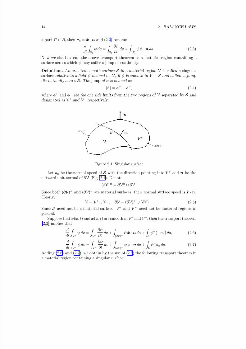
Definition. An oriented smooth surface S in a material region V is called a singularsurface relative to a field φ defined on V , if φ is smooth in V − S and suffers a jumpdiscontinuity across S . The jump of φ is defined as

[[φ]] = φ+ − φ−, (2.4)

where φ+ and φ− are the one side limits from the two regions of V separated by S and designated as

V + and

V − respectively.

n

S un

V − V +(∂ V )+

(∂ V )−

Figure 2.1: Singular surface

Let un be the normal speed of S with the direction pointing into V + and n be theoutward unit normal of ∂ V (Fig. 2.1). Denote

(∂ V )± = ∂ V ± ∩ ∂ V .Since both (∂ V )+ and (∂ V )− are material surfaces, their normal surface speed is x · n.Clearly,

V =

V +

∪ V −, ∂

V = (∂

V )+

∪(∂

V )−. (2.5)

Since S need not be a material surface, V + and V − need not be material regions ingeneral.

Suppose that ψ(x, t) and x(x, t) are smooth in V + and V −, then the transport theorem(2.2) implies that

d

dt

V +

ψ dv = V +

∂ψ

∂t dv + (∂ V )+

ψ x · n da + S

ψ+(−un) da, (2.6)

d

dt

V −

ψ dv = V −

∂ψ

∂t dv + (∂ V )−

ψ x · n da + S

ψ−un da. (2.7)

Adding (2.6) and (2.7), we obtain by the use of (2.5) the following transport theorem ina material region containing a singular surface:



2. LOCAL BALANCE EQUATION AND JUMP CONDITION 15

Theorem. Let V (t) be a material region in E and S (t) be a singular surface relative to the tensor field ψ(x, t) which is smooth elsewhere. Then we have

ddt V

ψ dv = V

∂ψ∂t

dv + ∂ V

ψ x · n da − S

[[ψ]] un da, (2.8)

where un(x, t) is the normal speed of a surface point x ∈ S (t) and [[ψ]] is the jump of ψacross S .

2.2 Local balance equation and jump condition

For a material region V containing a singular surface S , the equation of general balancein integral form (2.1) becomes

V

∂ψ

∂t dv + ∂ V

ψ x · n da − S

[[ψ]] un da = ∂ V

Φψn da + V

σψ dv. (2.9)

Definition. A point x is called regular if there is a material region containing x in whichall the tensor fields in ( 2.1) are smooth. And a point x is called singular if it is a pointon a singular surface relative to ψ and Φψ.

We can obtain the local balance equation at a regular point as well as at a singularpoint from the above integral equation. First, we consider a small material region V containing x such that V ∩ S = ∅. By the use of the divergence theorem, (2.9) becomes

V

∂ψ

∂t + div(ψ ⊗ x− Φψ) − σψ

dv = 0. (2.10)

Since the integrand is smooth and the equation (2.10) holds for any V , such that x ∈ V ,and V ∩ S = ∅, the integrand must vanish at x. Therefore we have

Theorem (local balance equation). At a regular point x, the general balance equation( 2.9 ) reduces to

∂ψ

∂t + div(ψ ⊗ x− Φψ) − σψ = 0. (2.11)

The notation div(ψ⊗ x) in (2.11) should be understood as div(ψ x) when ψ is a scalarquantity.

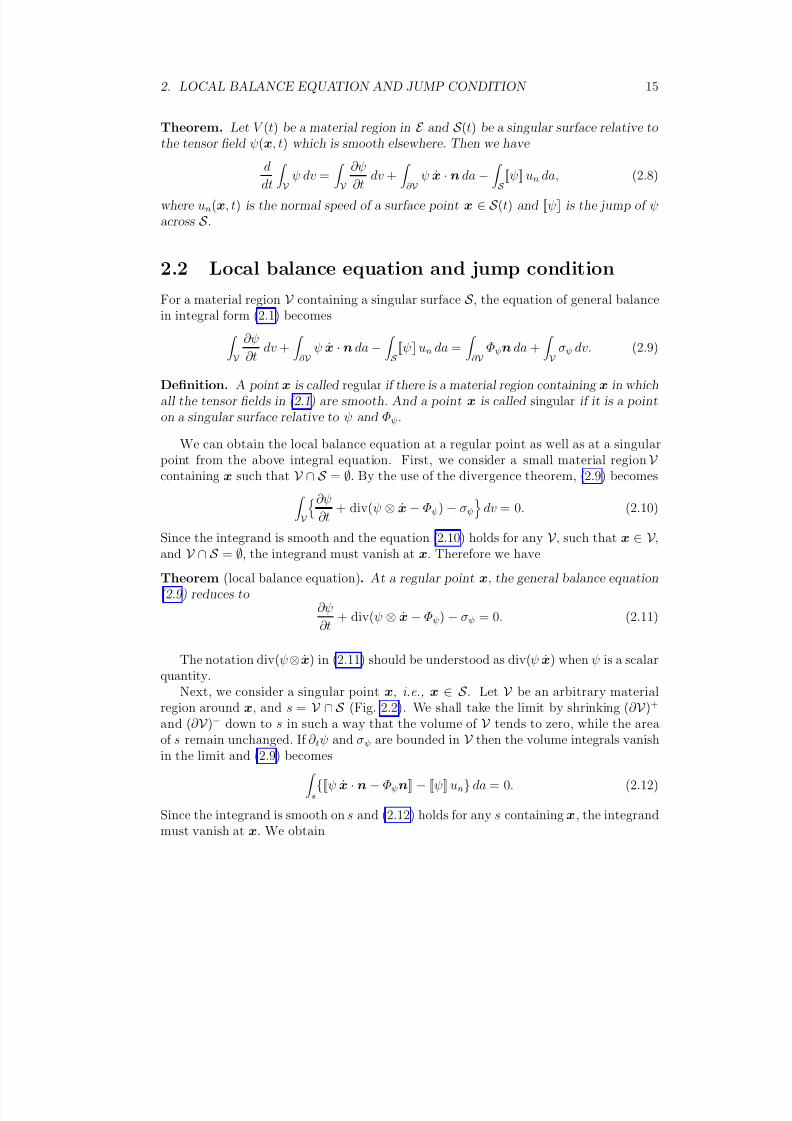
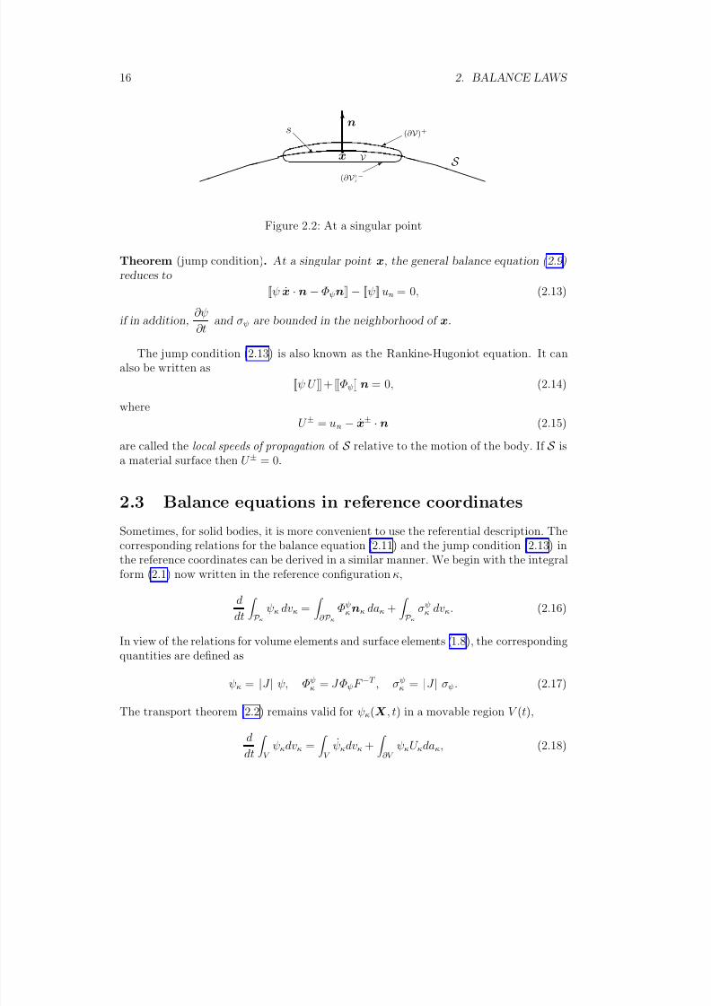
Next, we consider a singular point x, i.e., x ∈ S . Let V be an arbitrary materialregion around x, and s = V ∩ S (Fig. 2.2). We shall take the limit by shrinking (∂ V )+and (∂ V )− down to s in such a way that the volume of V tends to zero, while the areaof s remain unchanged. If ∂ tψ and σψ are bounded in V then the volume integrals vanishin the limit and (2.9) becomes

s{[[ψ x · n− Φψn]] − [[ψ]] un} da = 0. (2.12)

Since the integrand is smooth on s and (2.12) holds for any s containing x

, the integrandmust vanish at x. We obtain



16 2. BALANCE LAWS

x

V S

s n

(∂ V )+

(∂ V )−

Figure 2.2: At a singular point

Theorem (jump condition). At a singular point x, the general balance equation ( 2.9 )reduces to

[[ψ x · n− Φψn]] − [[ψ]] un = 0, (2.13)

if in addition, ∂ψ

∂t and σψ are bounded in the neighborhood of x.

The jump condition (2.13) is also known as the Rankine-Hugoniot equation. It canalso be written as

[[ψ U ]] + [[Φψ]]n = 0, (2.14)

where

U ± = un − x± · n (2.15)

are called the local speeds of propagation of S relative to the motion of the body. If S isa material surface then U ± = 0.

2.3 Balance equations in reference coordinates

Sometimes, for solid bodies, it is more convenient to use the referential description. Thecorresponding relations for the balance equation (2.11) and the jump condition (2.13) inthe reference coordinates can be derived in a similar manner. We begin with the integralform (2.1) now written in the reference configuration κ,

d

dt

P κ

ψκ dvκ = ∂ P κ

Φψκnκ daκ + P κ

σψκ dvκ. (2.16)

In view of the relations for volume elements and surface elements (1.8), the correspondingquantities are defined as

ψκ = |J | ψ, Φψκ = J ΦψF −T , σψ

κ = |J | σψ. (2.17)

The transport theorem (2.2) remains valid for ψκ(X , t) in a movable region V (t),

ddt V

ψκdvκ = V

ψκdvκ + ∂V

ψκU κdaκ, (2.18)



4. CONSERVATION OF MASS 17

where U κ(X , t) is the outward normal speed of a surface point X ∈ ∂V (t). Therefore forsingular surface S κ(t) moving across a material region V κ in the reference configuration,

by a similar argument, we can obtain from (2.9) V κ

ψκdvκ − S κ

[[ψκ]] U κdaκ = ∂ V κ

Φψκnκdaκ + V κ

σψκ dvκ, (2.19)

where U κ is the normal speed of the surface points on S κ, while the normal speed of thesurface points on ∂ V κ is zero since a material region is a fixed region in the referenceconfiguration. From this equation, we obtain the local balance equation and the jumpcondition in the reference configuration,

ψκ − Div Φψκ − σψ

κ = 0, [[ψκ]] U κ + [[Φψκ ]]nκ = 0, (2.20)

where U κ and n

κ are the normal speed and the unit normal vector of the singular surface.

2.4 Conservation of mass

Let ρ(x, t) denote the mass density of Bt in the current configuration. Since the materialis neither destroyed nor created in any motion in the absence of chemical reactions, wehave

Conservation of mass. The total mass of any part P ⊂ B does not change in any motion,

d

dt P t ρ dv = 0. (2.21)

By comparison, it is a special case of the general balance equation (2.1) with no fluxand no supply,

ψ = ρ, Φψ = 0, σψ = 0,

and hence from (2.11) and (2.13) we obtain the local expressions for mass conservationand the jump condition at a singular point,

∂ρ

∂t + div(ρ x) = 0, [[ρ (x · n− un)]] = 0. (2.22)

The equation (2.21) states that the total mass of any part is constant in time. Inparticular, if ρκ(X ) denote the mass density of Bκ in the reference configuration, than

P κρκdvκ = P t

ρdv, (2.23)

which implies thatρκ = ρ |J |, (2.24)

where J = det F . This is another form of the conservation of mass in the referentialdescription, which also follows from the general expression (2.20) and (2.17).

We note that if the motion is volume-preserving, then

ddt P t

dv = 0,



18 2. BALANCE LAWS

which by comparison with (2.1) again leads to

div x = 0,

which in turn implies that ρ = 0 by (2.22)1. Therefore, for an incompressible motion,the mass density is time-independent and the divergence of velocity field must vanish.

2.5 Equation of motion

For a deformable body, the linear momentum and the angular momentum with respectto a point x◦ ∈ E of a part P ⊂ B in the motion can be defined respectively as

P t

ρ x dv, and P t

ρ (x− x◦) × x dv.

In laying down the laws of motion, we follow the classical approach developed byNewton and Euler, according to which the change of momentum is produced by theaction of forces. There are two type of forces, namely, one acts throughout the volume,called the body force , and one acts on the surface of the body, called the surface traction .

Euler’s laws of motion. Relative to an inertial frame, the motion of any part P ⊂ Bsatisfies

d

dt P t ρ x dv = P t ρ b dv + ∂ P t t da,

d

dt

P t

ρ (x− x◦) × x dv = P t

ρ (x− x◦) × b dv + ∂ P t

(x− x◦) × t da.

We remark that the existence of inertial frames (an equivalent of Newton’s first law)is essential to establish the Euler’s laws (equivalent of Newton’s second law) in the aboveforms. Roughly speaking, a coordinate system (x) at rest for E is usually regarded as aninertial frame. Euler’s laws in an arbitrary frame can be obtained through the notion of change of reference frames considered in Chapter 3.

We call b the body force density (per unit mass), and t the surface traction (per unit

surface area). Unlike the body force b = b(x, t), such as the gravitational force, thetraction t at x depends, in general, upon the surface ∂ P t on which x lies. It is obviousthat there are infinite many parts P ⊂ B, such that ∂ P t may also contain x. However,following Cauchy, it is always assumed in the classical continuum mechanics that thetractions on all like-oriented surfaces with a common tangent plane at x are the same.

Postulate (Cauchy). Let n be the unit normal to the surface ∂ P t at x, then

t = t(x, t,n). (2.25)

An immediate consequence of this postulate is the well-known theorem which ensuresthe existence of stress tensor.



6. CONSERVATION OF ENERGY 19

Theorem (Cauchy). Suppose that t(·,n) is a continuous function of x, and x, b are bounded in Bt. Then Cauchy’s postulate and Euler’s first law implies the existence of a

second order tensor T , such thatt(x, t,n) = T (x, t)n. (2.26)

The tensor field T (x, t) in (2.26) is called the Cauchy stress tensor . The proof of thetheorem can be found in most books of mechanics. The continuity assumption in thetheorem is often too stringent for the existence of stress tensor in some applications, forexample, problems involving shock waves. However, it has been shown that the theoremremains valid under a much weaker assumption of integrability, which would be satisfiedin most applications [7, 6].

With (2.26) Euler’s first law becomes

ddt P t

ρ x dv = P t

ρb dv + ∂ P t

T n da. (2.27)

Comparison with the general balance equation (2.1) leads to

ψ = ρ x, Φψ = T , σψ = ρ b,

in this case, and hence from (2.11) and (2.13) we obtain the balance equation of linearmomentum and its jump condition,

∂

∂t(ρ x) + div(ρ x⊗ x− T ) − ρ b = 0, [[ρ x(x · n− un)]] − [[T ]]n = 0. (2.28)

The first equation, also known as the equation of motion , can be rewritten in the followingmore familiar form by the use of (2.22),

ρ x− div T = ρ b. (2.29)

A similar argument for Euler’s second law as a special case of ( 2.1) with

ψ = (x− x◦) × ρ x, Φψn = (x− x◦) × T n, σψ = (x− x◦) × ρ b,

leads toT = T T , (2.30)

after some simplification by the use of (2.29). In other words, the symmetry of the stresstensor is a consequence of the conservation of angular momentum.

2.6 Conservation of energy

Besides the kinetic energy, the total energy of a deformable body consists of another partcalled the internal energy,

P t

ρ ε +

ρ

2 x · x

dv,

where ε(x, t) is called the specific internal energy density . The rate of change of the totalenergy is partly due to the mechanical power from the forces acting on the body andpartly due to the energy inflow over the surface and the external energy supply.



20 2. BALANCE LAWS

Conservation of energy. Relative to an inertial frame, the change of energy for any part P ⊂ B is given by

d

dt

P t

(ρ ε + ρ

2 x · x) dv = ∂ P t

(x · T n− q · n) da + P t

(ρ x · b + ρ r) dv. (2.31)

We call q(x, t) the heat flux vector (or energy flux), and r(x, t) the energy supply

density due to external sources, such as radiation. Comparison with the general balanceequation (2.1), we have

ψ = (ρ ε + ρ

2 x · x), Φψ = T x− q, σψ = ρ (x · b + r),

and hence we have the following local balance equation of total energy and its jumpcondition,

∂

∂t

ρ ε +

ρ

2 x · x

+ div

(ρ ε + ρ

2 x · x)x + q − T x

= ρ (r + x · b),

[[(ρ ε + ρ

2 x · x)(x · n− un)]] + [[q − T x]] · n = 0.

(2.32)

The energy equation (2.32)1 can be simplified by substracting the inner product of theequation of motion (2.29) with the velocity x,

ρ ε + div q = T · grad x + ρ r. (2.33)

This is called the balance equation of internal energy. Note that the internal energy isnot conserved and the term T · grad x is the rate of work due to deformation.

Summary of basic equations:

By the use of material time derivative (1.22), the field equations can also be written asfollows:

ρ + ρ div v = 0,ρ v − div T = ρ b,

ρ ε + div q − T · gradv = ρ r,

(2.34)

and the jump conditions in terms of local speed U of the singular surface become

[[ρ U ]] = 0,

[[ρ U v]] + [[T ]]n = 0,

[[ρ U (ε + 1

2v2)]] + [[T v − q]] · n = 0,

(2.35)

where v2 stands for v · v.



7. BASIC EQUATIONS IN MATERIAL COORDINATES 21

2.7 Basic Equations in Material Coordinates

It is sometimes more convenient to rewrite the basic equations in material descriptionrelative to a reference configuration κ. They can easily be obtained from (2.20)1,

ρ = |J |−1ρκ,

ρκx = Div T κ + ρκb,

ρκ ε + Div qκ = T κ · F + ρκr,

(2.36)

where the following definitions have been introduced according to (2.17):

T κ = J T F −T , qκ = J F −1q. (2.37)

T κ is called the Piola–Kirchhoff stress tensor and qκ is called the material heat flux .

Note that unlike the Cauchy stress tensor T , the Piola–Kirchhoff stress tensor T κ is notsymmetric and it must satisfy

T κF T = F T T κ . (2.38)

The definition has been introduced according to the relation (1.8), which gives the rela-tion,

S T n da = S κ

T κnκdaκ. (2.39)

In other words, T n is the surface traction per unit area in the current configuration,while T κnκ is the surface traction measured per unit area in the reference configuration.Similarly, q

·n and qκ

·nκ are the contact heat supplies per unit area in the current and

the reference configurations respectively.We can also write the jump conditions in the reference configuration by the use of

(2.20)2,[[ρκ]] U κ = 0,

[[ρκ x]] U κ + [[T κ]]nκ = 0,

[[ρκ(ε + 1

2 x · x)]] U κ + [[T T κ x− qκ]] · nκ = 0,

(2.40)

where nκ and U κ are the unit normal and the normal speed at the singular surface inthe reference configuration.

2.8 Boundary conditions of a material body

The boundary of a material body is a material surface. Therefore, U ± = 0 at theboundary ∂ Bt, the jump conditions (2.35) of linear momentum and energy become

[[T ]]n = 0,

[[q]] · n = [[v · T n]].

Suppose that the body is acted on the boundary by an external force f per unitarea of the boundary ∂ Bt, then it requires the stress to satisfy the traction boundary

condition, T n = f , (2.41)



22 2. BALANCE LAWS

and the heat flux to satisfy[[q]] · n = [[v]] · f .

In particular, if either the boundary is fixed (v = 0) or free (f = 0) then the normalcomponent of heat flux must be continuous at the boundary,

[[q]] · n = 0. (2.42)

Therefore, if the body has a fixed adiabatic (meaning thermally isolated) boundary thenthe normal component of the heat flux must vanish at the boundary.

Since the deformed configuration is usually unknown for traction boundary valueproblems of a solid body, the above conditions, which involved the unknown boundary,are sometimes inconvenient.

Of course, we can also express the boundary conditions in the reference configuration.From the jump conditions (2.40)2,3, we have

T κnκ = f κ, qκ · nκ = hκ, (2.43)

where f κ and hκ are the force and the normal heat flux per unit area acting on the fixedboundary ∂ Bκ, respectively. These are the usual boundary conditions in elasticity andheat conduction.

In case the traction boundary condition is prescribed in the deformed configuration∂ Bt, instead of in the reference configuration ∂ Bκ, we need to pull back the boundaryforce f (x, t) to f κ(X , t). In deed, we have

S f da = S κf κdaκ, f κ =

da

daκf ,

for S κ ⊂ ∂ Bκ and the corresponding S ⊂ ∂ Bt.In order to obtain an expression for the area ratio, we start with the relation ( 1.8)

n da = J F −T nκdaκ,

from which, it follows

n = F −T nκ

|F −T nκ| , nκ = F T n

|F T n| , (2.44)

and with (2.44)2 the above relation becomes

n da = J

|F T n

|n daκ.

Therefore, we have

da = J

|F T n| daκ = det F √ F T n · F T n

daκ.

Similarly, with (2.44)1, we have

da = J |F −T nκ| daκ = (det F )

F −T nκ · F −T nκ daκ.

and hence, we obtain

da

daκ=

det F √ n · Bn

= (det F ) nκ · C −1nκ, (2.45)

where B and C are the left and the right Cauchy–Green strain tensors.



CHAPTER 3

Constitutive Relations

The balance laws introduced in Chapter 2 are the fundamental equations which are com-mon to all material bodies. However, these laws are not sufficient to fully characterize thebehavior of material bodies, because physical experiences have shown that two samples of exactly the same size and shape in general will not have the same behavior when they are

subjected to exactly the same experiment (external supplies and boundary conditions).Mathematically, the physical properties of a body can be given by a description of

constitutive relations. These relations characterize the material properties of the body. Itis usually assumed that such properties are intrinsic to the material body and, therefore,must be independent of external supplies as well as of different observers that happen tobe measuring the material response simultaneously.

By an observer we mean a frame of reference for the event world and therefore isable to measure the position in the Euclidean space and time on the real line. Theconfiguration of a body introduced so far should have been defined relative to a givenframe of reference, but since only a given frame is involved, the concept of frame has

been set aside until now when a change of frame of reference becomes essential in laterdiscussions.

3.1 Frame of reference, observer

The space-time W is a four-dimensional space in which events occur at some places andcertain instants. Let W t be the space of placement of events at the instant t, then inNewtonian space-time of classical mechanics, we can write

W =t∈IR

W t,

and regard W as a product space E × IR, where E is a three dimensional Euclidean spaceand IR is the space of real numbers, through a one-to one mapping, called a frame of

reference (see [21]),φ : W → E × IR,

such that it gives rise to a one-to-one mapping for the space of placement into theEuclidean space,

φt : W t → E . (3.1)

The frame of reference φ can usually be referred to as an observer , since it can bedepicted as taking a snapshot of events at some instant t with a camera, so that the image



24 3. CONSTITUTIVE RELATIONS

of φt is a picture (three-dimensional conceptually) of the placement of events, from whichthe distance between different simultaneous events can be measured physically, with a

ruler for example. Similarly, an observer can record a sequence of snapshots at differentinstants with a video camera for the change of events in time.

Motion of a body

The motion of a body can be viewed as a sequence of events such that at any instant t,the placement of the body B in W t is a one-to-one mapping

χt : B → W t,

which relative to a frame of reference φt : W t → E can be described as

χφt : B → E , χφt := φt ◦ χt, x = χφt( p) ∀ p ∈ B,

which identifies the body with a region in the Euclidean space. We call χφt a configuration

of B at the instant t in the frame φ, and a motion of B is a sequence of configurations of B in time,

χφ = {χ

φt, t ∈ IR | χφt : B → E}.

Reference configuration

As a primitive concept, a body B is considered to be a set of material points withoutadditional mathematical structures. Although it is possible to endow the body as amanifold with a differentiable structure and topology,1 for doing mathematics on thebody, usually a reference configuration , say

κφ : B → E , X = κφ( p), Bκφ := κφ(B),

is chosen, so that the motion can be treated as a function defined on the Euclideanspace E ,

χκφ(·, t) : Bκφ ⊂ E → E , x = χ

κφ(X , t) ∀X ∈ Bκφ.

For examples, in previous chapters, we have already introduced

x(X , t) = ∂ χκφ(X , t)

∂t , x(X , t) = ∂

2χκφ(X , t)∂t2

,

andF κ(X , t) = ∇XX X

χκφ(X , t),

called the velocity, the acceleration, and the deformation gradient of the motion, respec-tively. Note that no explicit reference to κφ is indicated in these quantities for brevity,unless similar notations reference to another frames are involved.

Remember that a configuration is a placement of a body relative to an observer,therefore, for the reference configuration κφ, there is some instant, say t0 (not explicitly

1

Mathematical treatment of a body as a differentiable manifold is beyond the scope of the presentconsideration (see [26]).



2. CHANGE OF FRAME AND OBJECTIVE TENSORS 25

indicated for brevity), at which the reference placement of the body is made. On theother hand, the choice of a reference configuration is arbitrary, and it is not necessary that

the body should actually occupy the reference place in its motion under consideration.Nevertheless, in most practical problems, t0 is usually taken as the initial time of themotion.

3.2 Change of frame and objective tensors

Now suppose that two observers, φ and φ∗, are recording the same events with videocameras. In order to be able to compare the pictures from different viewpoints of theirrecordings, two observers must have a mutual agreement that the clocks of their cameramust be synchronized so that simultaneous events can be recognized, and, since during the

recording two people may move independently while taking pictures with different anglesfrom their camera, there will be a relative motion and a relative orientation betweenthem. These facts, can be expressed mathematically as follows:

We call ∗ := φ∗ ◦ φ−1,

∗ : E × IR → E × IR, ∗(x, t) = (x∗, t∗),

a change of frame (observer), where (x, t) and (x∗, t∗) are the position and time of thesimultaneous events observed by φ and φ∗ respectively. From the observers’ agreement,they must be related in the following manner,

x∗ = Q(t)(x− x0) + c(t)t∗ = t + a,

(3.2)

for some x0, c(t) ∈ E , Q(t) ∈ O(V ), a ∈ IR, where O(V ) is the group of orthogonaltransformations on the translation space V of the Euclidean space E . In other words, achange of frame is an isometry of space and time as well as preserves the sense of time.Such a transformation will be called a Euclidean transformation .

In particular, φ∗t ◦ φ−1

t : E → E is given by

x∗ = φ∗t (φ−1

t (x)) = Q(t)(x− xo) + c(t), (3.3)

which is a time-dependent rigid transformation consisting of an orthogonal transforma-tion and a translation. We shall often call Q(t) as the orthogonal part of the change of frame from φ to φ∗.

Objective tensors

The change of frame (3.2) on the Euclidean space E gives rise to a linear mapping onthe translation space V , in the following way: Let u(φ) = x2 −x1 ∈ V be the differencevector of x1,x2 ∈ E in the frame φ, and u(φ∗) = x∗2 − x∗

1 ∈ V be the correspondingdifference vector in the frame φ∗, then from (3.2)1, it follows immediately that

u(φ∗) = Q(t)u(φ).




Any vector quantity in V , which has this transformation property, is said to be objectivewith respect to Euclidean transformations. The Euclidean objectivity can be generalized

to any tensor spaces of V . In particular, we have the following definition.

Definition. Let s, u, and T be scalar-, vector-, (second order) tensor-valued functions respectively. If relative to a change of frame from φ to φ∗ given by any Euclideantransformation,

s(φ∗) = s(φ),

u(φ∗) = Q(t)u(φ),

T (φ∗) = Q(t) T (φ) Q(t)T ,

where Q(t) is the orthogonal part of the change of frame, then s, u and T are called objective scalar, vector and tensor quantities respectively. They are also said to be frame-

indifferent (in the change of frame with Euclidean transformation) or simply Euclideanobjective.

We call f (φ) the value of the function observed in the frame of reference φ, and forsimplicity, write f = f (φ) and f ∗ = f (φ∗).

The definition of objective scalar is self-evident, while for objective tensors, thedefinition becomes obvious if one considers a simple tensor T = u ⊗ v, by defining(u⊗ v)(φ) = u(φ) ⊗ v(φ) and hence

(u⊗ v)(φ∗) = u(φ∗) ⊗ v(φ∗)

= Q(t)u(φ) ⊗ Q(t)v(φ) = Q(t)((u⊗ v)(φ))Q(t)T ,

as the relation between the corresponding linear transformations observed by the twoobservers.

One can easily deduce the transformation properties of functions defined on the posi-tion and time. Consider an objective scalar field ψ(x, t) = ψ∗(x∗, t∗). Taking the gradientwith respect to x, from (3.3) we obtain

∇xxxψ(x, t) = Q(t)T ∇xxx∗ψ∗(x∗, t∗),

or

(grad ψ)(φ∗) = Q(t)(grad ψ)(φ), (3.4)

which proves that grad ψ is an objective vector field. Similarly, we can show that if uis an objective vector field then gradu is an objective tensor field. However, one caneasily show that the partial derivative ∂ψ/∂t is not an objective scalar field and neitheris ∂ u/∂t an objective vector field.

Proposition. Let a surface be given by f (x, t) = 0, and

n(x, t) = ∇xxxf

|∇xxxf

|be the unit normal to the surface. Then n is an objective vector field.




Proof . In the change of frame, we can write for the surface,

f ∗(x∗, t∗) = f ∗(x∗(x, t), t∗(t)) = f (x, t) = 0.

By taking gradient with respect to x, we obtain, from (3.4) that

QT ∇xxx∗f ∗ = ∇xxxf,

from which, since Q is orthogonal, |QT ∇xxx∗f ∗| = |∇xxx∗f ∗|, it follows that

n∗ = Qn. (3.5)

Transformation properties of motion

Let χφ be a motion of the body in the frame φ, and χ

φ∗ be the corresponding motionin φ∗,

x = χφt( p) = χ( p, t), x∗ = χ

φ∗t( p) = χ∗( p, t∗), p ∈ B.

Then from (3.3), we have

χ∗( p, t∗) = Q(t)(χ( p, t) − xo) + c(t), p ∈ B. (3.6)

Consequently, the transformation property of a kinematic quantity, associated with the

motion in E , can be derived from (3.6). In particular, one can easily show that thevelocity and the acceleration are not objective quantities. Indeed, it follows from (3.6)that

x∗ = Qx + Q(x− xo) + c,

x∗ = Qx + 2 Qx + Q(x− x0) + c.(3.7)

The relation (3.7)2 shows that x is not objective but it also shows that x is an objectivetensor with respect to transformations for which Q(t) is a constant tensor. A change of frame with constant Q(t) and c(t) linear in time t is called a Galilean transformation .Therefore, we conclude that the acceleration is a Galilean objective tensor quantity but

not a Euclidean objective one. However, from (3.7)1, it shows that the velocity is neithera Euclidean nor a Galilean objective vector quantity.

Transformation properties of deformation

Let κ : B → W t0 be a reference placement of the body at some instant t0, then

κφ = φt0 ◦ κ and κφ∗ = φ∗t0

◦ κ (3.8)

are the two corresponding reference configurations of B in the frames φ and φ∗ at thesame instant (see Fig. 3.1), and

X = κφ( p), X ∗ = κφ∗( p), p ∈ B.




W t0

B

Bκ ⊂ E Bκ∗ ⊂ E

γ

κφ κφ∗κ

φt0 φ∗t0

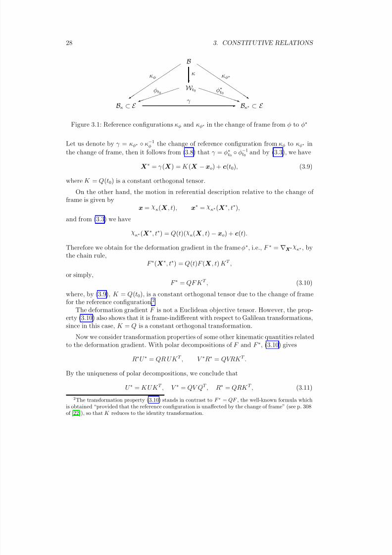
Figure 3.1: Reference configurations κφ and κφ∗ in the change of frame from φ to φ∗

Let us denote by γ = κφ∗ ◦ κ−1φ the change of reference configuration from κφ to κφ∗ in

the change of frame, then it follows from (3.8) that γ = φ∗t0

◦ φ−1t0 and by (3.3), we have

X ∗ = γ (X ) = K (X −xo) + c(t0), (3.9)

where K = Q(t0) is a constant orthogonal tensor.

On the other hand, the motion in referential description relative to the change of frame is given by

x = χκ(X , t), x∗ = χ

κ∗(X ∗, t∗),

and from (3.3) we have

χκ∗(X ∗, t∗) = Q(t)(χ

κ(X , t) − xo) + c(t).

Therefore we obtain for the deformation gradient in the frame φ∗, i.e., F ∗ = ∇XX X ∗χκ∗ , bythe chain rule,

F ∗(X ∗, t∗) = Q(t)F (X , t) K T ,

or simply,F ∗ = QF K T , (3.10)

where, by (3.9), K = Q(t0), is a constant orthogonal tensor due to the change of framefor the reference configuration.2

The deformation gradient F is not a Euclidean objective tensor. However, the prop-erty (3.10) also shows that it is frame-indifferent with respect to Galilean transformations,

since in this case, K = Q is a constant orthogonal transformation.

Now we consider transformation properties of some other kinematic quantities relatedto the deformation gradient. With polar decompositions of F and F ∗, (3.10) gives

R∗U ∗ = QR UK T , V ∗R∗ = QVRK T .

By the uniqueness of polar decompositions, we conclude that

U ∗ = K UK T , V ∗ = QV QT , R∗ = QRK T , (3.11)

2The transformation property (3.10) stands in contrast to F ∗ = QF , the well-known formula which

is obtained “provided that the reference configuration is unaffected by the change of frame” (see p. 308of [22]), so that K reduces to the identity transformation.




and alsoC ∗ = K CK T , B∗ = QBQT . (3.12)

Therefore, R, U , and C are not objective tensors, but the tensors V and B are objective.If we differentiate (3.10) with respect to time, we obtain

F ∗ = Q F K T + QF K T .

With L = grad x = F F −1 by (1.24), we have

L∗F ∗ = QLF K T + QF K T = QLQT F ∗ + QQT F ∗,

and since F ∗ is non-singular, it gives

L∗ = QLQT + QQT . (3.13)

Moreover, with L = D + W , it becomes

D∗ + W ∗ = Q(D + W )QT + QQT .

By separating symmetric and skew-symmetric parts, we obtain

D∗ = QDQT , W ∗ = QW QT + QQT , (3.14)

since QQT is skew-symmetric. Therefore, while the velocity gradient grad x and the spintensor W are not objective, the rate of strain tensor D is an objective tensor.

Objective time derivatives

Let ψ and u be objective scalar and vector fields respectively,

ψ∗(X ∗, t∗) = ψ(X , t), u∗(X ∗, t∗) = Q(t)u(X , t).

It follows thatψ∗ = ψ, u∗ = Qu + Qu.

Therefore, the material time derivative of an objective scalar field is objective, while thematerial time derivative of an objective vector field is not longer objective.

Nevertheless, we can define an objective time derivatives of vector field in the followingway: Let P t(τ ) : V → V be a transformation which takes a vector at time t to a vectorat time τ and define the time derivative as

DP tu(t) = limh→0

1

h(u(t + h) − P t(t + h)u(t)), (3.15)

so that the vector u(t) is transformed to a vector at (t + h) through P t(t + h) in order tobe compared with the vector u(t + h) at the same instant of time. This is usually calleda Lie derivative.

Now, we shall take P t(τ ) to be the relative rotation tensor of the motion Rt(τ ) (see

(1.30)) and denote ◦u= DRtu.




Since

Rt(t + h) = Rt(t) + Rt(t)h + o(2)

and from (1.32)

Rt(t) = 1, Rt(t) = W (t),

we have◦u(t) = lim

h→0

1

h(u(t + h) − u(t) − h W (t)u(t)),

or◦u= u− W u. (3.16)

Note that by (3.14)2,

( ◦u)∗ = u∗ − W ∗u∗

= Qu + Qu− (QW QT + QQT )Qu

= Q( u− W u) = Q ◦u .

Therefore, ◦u is an objective time derivative of u. This derivative is called the corotational

time derivative , which measures the time rate of change experienced by material particlesrotating along with the motion.

Similarly, if we take P t(τ ) to be the relative deformation gradient of the motion F t(τ )(see (1.30)) and denote

u = DF tu.

It is an called the convected time derivatives , which measures the time rate of changeexperienced by material particles carried along with the motion. It follows that

u = u− Lu,

which is also an objective time derivative.

For an objective tensor field S , we can define

DP tS (t) = limh→0

1h

(S (t + h) − P t(t + h)S (t)P t(t + h)T ), (3.17)

and let◦S = DRtS,

S = DF tS,

which define the objective corotational and convective time derivative of an objectivetensor field S as

◦

S = S − W S + SW,

S = S

−LS

−SLT ,

respectively.



3. CONSTITUTIVE RELATIONS 31

3.3 Constitutive relations

Physically the thermomechanical behavior of a body is characterized by a descriptionof the fields of density ρ( p, t), motion χ( p, t) and temperature θ( p, t), called the basicthermodynamic fields. The material response of a body generally depends on the pasthistory of its thermomechanical behavior.

Let us introduce the notion of the past history of a function. Let h(·) be a functionof time. The history of h up to time t is defined by

ht(s) = h(t − s), (3.18)

where s ∈ [0, ∞) denotes the time-coordinate pointed into the past from the presenttime t. Clearly s = 0 corresponds to the present time, therefore

ht(0) = h(t).

Mathematical descriptions of material response are called constitutive relations or con-stitutive equations. We postulate that the history of the behavior up to the present timedetermines the response of the body.

Principle of determinism (in material description). Let φ be a frame of reference, and C be a constitutive quantity, then the constitutive relation for C is given by a functional of the form,3

C( p, t) = F φ pp p∈B0≤s<∞

(ρt

( p

, s), χt

( p

, s), θt

( p

, s), t ; p), p ∈ B, t ∈ IR. (3.19)

We call F φ the constitutive function or response function of C in the frame φ. Note thatwe have indicated the domains of the argument functions as underscripts in the notationof the functional F φ. Such a functional allows the description of arbitrary non-local effectof any inhomogeneous body with a perfect memory of the past thermomechanical history.With the notation F φ, we emphasize that the value of a constitutive function a priori

may depend on the observer (frame of reference φ) who is measuring the response of thematerial body and the material point p.

Constitutive relations can be regarded as mathematical models of material bodies.The validity of a model can be verified by experiments. However, experiments alone arerarely sufficient to determine constitutive functions of a material body. Nevertheless,there are some universal requirements that a model should obey lest its consequences becontradictory to some well-known physical experiences. Therefore, in search of a correct

3 The functional F φ can be expressed more directly as

C( p, t) = F φ(ρt, χt, θt, t ; p),

where the first three arguments are functions:

ρt :

B×[0,

∞)

→ IR, χt :

B ×[0,

∞)

→ E , θt :

B ×[0,

∞)

→ IR.




formulation of a mathematical model in general, we shall first impose these requirementson the proposed model. The most important universal requirements of this kind are

– Euclidean objectivity,– principle of material frame-indifference,– material symmetry,– thermodynamic considerations.

Euclidean objectivity, principle of material frame-indifference and material symmetry willbe discussed in this chapter and a brief account of thermodynamic considerations will begiven later. These requirements impose severe restrictions on the model and hence leadto a great simplification for general constitutive relations. The reduction of constitutiverelations from very general to more specific and mathematically simpler ones for a givenclass of materials is the main objective of constitutive theories in continuum mechanics.

3.4 Euclidean objectivity

In addition to the conservation laws in an inertial frame stated in the previous chapter,we should have also postulated that the mass density, the internal energy (but not thetotal energy) and the temperature are objective scalar quantities, while the heat flux andthe surface traction are objective vector quantities, so that the conservation laws relativeto an arbitrary frame of reference can be deduced (see [14]).

In particular, under a change of frame, we have t∗ = Qt for the surface traction andsince t = T n, and n∗ = Qn from (3.5), it follows that the stress T is an objective tensorquantity. To emphasize the objectivity postulate in the conservation laws, it is referredto as Euclidean objectivity of constitutive quantities:

Euclidean objectivity. The constitutive quantities: the stress T , the heat flux q and the internal energy density ε, are objective with respect to any Euclidean change of frame,

T ∗( p, t∗) = Q(t) T ( p, t) Q(t)T ,

q∗( p, t∗) = Q(t)q( p, t),

ε∗( p, t∗) = ε( p, t),

(3.20)

where Q(t) is the orthogonal part of the change of frame.Note that this postulate is a universal requirement in order to formulate the conservationlaws of material bodies in an arbitrary frame of reference, and no constitutive assumptionsare involved in the postulate of Euclidean objectivity.4

Let C = {T, q, ε} be constitutive quantities and φ be a frame of reference. Then from(3.19), the constitutive relations can be written as

C( p, t) = F φ(ρt, χt, θt, t ; p), p ∈ B, t ∈ IR, (3.21)

4In early writings of Truesdell and Noll (see [22]), this postulate was stated as part of the principle

of material frame-indifference. It would be much clear conceptually, if it were stated independently,because constitutive equations are irrelevant in this assumption.



5. PRINCIPLE OF MATERIAL FRAME INDIFFERENCE 33

where F φ is a functional with argument functions ρt, χt, θt, defined on B×[0, ∞), stand forthe past histories up to the instant t. Similarly, relative to the frame φ∗, the corresponding

constitutive relation can be written asC∗( p, t∗) = F φ∗

(ρt)∗, (χt)∗, (θt)∗, t∗; p

, p ∈ B, t∗ ∈ IR. (3.22)

The two constitutive functions F φ and F φ∗ are not independent, they must satisfy theEuclidean objectivity relation (3.20). In particular, for the stress, the condition (3.20)implies that

F φ∗((ρt)∗, (χt)∗, (θt)∗, t∗ ; p) = Q(t) F φ(ρt, χt, θt, t ; p) Q(t)T , (3.23)

for any histories

(ρ

t

)

∗

( p

, s) = ρ

∗

( p

, t

∗

− s) = ρ( p

, t − s),(θt)∗( p, s) = θ∗( p, t∗ − s) = θ( p, t − s),

(χt)∗( p, s) = Q(t − s)(χt( p, s) − xo) + c(t − s),

p ∈ B, (3.24)

where Q(t) ∈ O(V ), xo, c(t) ∈ E are associated with the change of frame from φ to φ∗.The first two relations of (3.24) state that the density and the temperature are ob-

jective scalar field as assumed and the last relation follows from (3.3).The relation (3.23) will be referred to as the “condition of Euclidean objectivity”

of constitutive functions, and can be regarded as the definition of the F φ∗ once theconstitutive function F φ is given5.

3.5 Principle of material frame indifference

The essential idea of the principle of material frame-indifference is that material proper-ties are frame-indifferent, i.e., material properties must be independent of observers. Thisstatement only makes sense when applies to constitutive quantities that are themselvesframe-indifferent, i.e., they must be objective quantities.

Since any intrinsic property of a material should be independent of observers, wepostulate that for any objective constitutive quantity, its constitutive function must bethe same in any frame.

Principle of material frame-indifference. The response function of an objective (frame-indifferent with respect to the Euclidean transformations) constitutive quantity C,in material description defined by ( 3.21) and ( 3.22 ), must be independent of the frame,i.e., for any frames of reference φ and φ∗

F φ( • ; p) = F φ∗( • ; p), p ∈ B. (3.25)

5For example, consider T = F φ(ρ, L). Since by Euclidean objectivity, ρ∗ = ρ, T ∗ = QT QT , and from

(3.13), L∗ = QLQT + QQT , it follows that

T ∗ = Q F φ(ρ, L) QT

= Q

F φ(ρ∗, QT L∗Q

−QT Q) QT := F

φ(ρ∗, L∗; Q, Q) :=

F φ∗(ρ∗, L∗),

where F φ∗, defined in the above relation, depends explicitly on Q(t) of the change of frame φ → φ∗.




We emphasize that the “form-invariance” (3.25) of constitutive function stated aboveis valid only when the material description is used so that the constitutive functions

characterize the material properties independent of any reference configuration. Theimplication in referential descriptions will be considered later. Moreover, for a non-objective constitutive quantity, such as the total energy, since the quantity itself is frame-dependent, it is obvious that its response function can never be independent of the frame.

In our discussions, we shall often consider only the constitutive function of stress, anobjective tensor quantity, for simplicity. Similar results can easily be obtained for anyother vector or scalar objective constitutive quantities.

Thus, from the condition of Euclidean objectivity (3.23) and the principle of materialframe-indifference (3.25), we obtain the following condition:

Condition of material objectivity. The response function of an objective tensor constitutive quantity, in material description, satisfies the condition,

F φ((ρt)∗, (χt)∗, (θt)∗, t∗, p) = Q(t) F φ(ρt, χt, θt, t ; p) Q(t)T , (3.26)

for any histories related by ( 3.24 ) where the change of frame from φ is arbitrary.

Since the condition (3.26) involves only the constitutive function in the frame φ, itbecomes a restriction imposed on the constitutive function F φ.

We emphasize that in the condition of Euclidean objectivity (3.23), Q(t) is the or-thogonal part of the change of frame from φ to φ∗. However, the condition of materialobjectivity is valid for an arbitrary change of frame from φ. Therefore, the condition(3.26) is valid for any Q(t) ∈ O(V ).

Sometimes, the condition of material objectivity is referred to as the “ principle of material objectivity”, to impart its relevance in characterizing material property andEuclidean objectivity, as a more explicit form of the principle of material-frame indiffer-ence.

An immediate restriction imposed by the condition of material objectivity can beobtained by considering a change of frame given by (Q(t) = 1, c(t) = x0)

x∗ = x, t∗ = t + a,

for arbitrary constant a ∈ IR. By (3.24), the condition (3.26) implies that

F φ(ρt, χt, θt, t + a ; p) = F φ(ρt, χt, θt, t ; p).

Since this is true for any value of a ∈ IR, we conclude that F φ can not depend on theargument t and the constitutive equations in general can be expressed as

C( p, t) = F φ(ρt, χt, θt; p), p ∈ B, t ∈ IR.






3.6 Simple material bodies

According to (3.19), thermomechanical histories of any part of the body can affect theresponse at any point of the body. In most applications, such a non-local property isirrelevant. Therefore it is usually assumed that only thermomechanical histories in anarbitrary small neighborhood of X ∈ Bκ affects the material response at the point X ,and hence the histories can be approximated at X by Taylor series up to certain order.In particular, when only linear approximation is concerned, in referential description theconstitutive relation (3.19) can be written as

C(X , t) = Hκ0≤s<∞

(χtκ(X , s), F t(X , s), θt(X , s), gt(X , s);X ), (3.31)

where g = grad θ is the spatial gradient of temperature. Note that since

ρ(X , t) = ρκ(X )

|det F (X , t)| ,

the functional dependence of (3.19) on ρt is absorbed into the dependence of (3.31) on X

and F t(X , s).A material body with constitutive relation defined by (3.31) is called a simple material

body . The class of simple materials, introduced by Noll [18], is general enough to includemost of the materials of practical interests, such as: the elastic solids, thermoelasticsolids, viscoelastic solids as well as elastic fluids, Navier-Stokes fluids and viscous heat-

conducting fluids.

An immediate consequence of the condition of material objectivity (3.30) can beobtained by the following choices of change of frame. Consider a change of frame givenby (Q(t) = 1, a = 0)

x∗ = x + c(t) − x0, t∗ = t.

Clearly, we haveχκ∗(γ (X ), t) = χ

κ(X , t) + (c(t) − x0),

and the condition (3.30) implies that

Hκ(χtκ + ct − x0, F t,X ) = Hκ(χt

κ, F t,X ).

Since (ct(s) − x0) ∈ V is arbitrary, we conclude that Hκ can not depend on the historyof position χt

κ(X , s).

Therefore, the constitutive relation of a simple material body in general is given by

C(X , t) = Hκ0≤s<∞

(F t(X , s), θt(X , s),gt(X , s);X ). (3.32)

It is important to point out that constitutive functions can not depend on the position

x nor on the velocity x, and indeed this can be proved for any materials in general as aconsequence of the principle of material objectivity (3.26).



7. MATERIAL SYMMETRY 37

For simple materials, the consequence of form-invariance (3.28) by the use of (3.9)takes the form

Hκ∗((F t

)∗

;X

∗

) = Hκ((F t

)∗

K ;X ), (3.33)and the Euclidean objectivity condition (3.29) becomes

Hκ∗((F t)∗;X ∗) = Q(t) Hκ(F t;X ) Q(t)T .

Combining the above two conditions and knowing the relation F ∗K = (QF K T )K = QF ,we obtain the following condition,7

Hκ(QtF t;X ) = Q(t) Hκ(F t;X ) Q(t)T . (3.34)

More generally, we have the following conditions for objective constitutive functionsof simple materials:

Condition of material objectivity. Constitutive functions for simple materials mustsatisfy the following conditions, for objective tensor, vector and scalar constitutive quan-tities respectively,

T (QtF t, θt, Qtgt;X ) = Q T (F t, θt, gt;X ) QT ,

Q(QtF t, θt, Qtgt;X ) = Q Q(F t, θt, gt;X ),

E (QtF t, θt, Qtgt;X ) = E (F t, θt, gt;X ),

∀ Q ∈ O(V ), (3.35)

and for any thermomechanical histories (F t, θt, gt).

These conditions are the restriction imposed on the constitutive functions by the require-

ment of material objectivity.Note that in condition (3.35), no mention of change of frame is involved, and Q(t)

can be interpreted as a superimposed orthogonal transformation on the deformation.This interpretation is sometimes viewed as an alternative version of the principle of material objectivity, and is called the “principle of invariance under superimposed rigid

body motions ”.

3.7 Material symmetry

We shall consider homogeneous simple material bodies in this section. A body is called

homogeneous if there is a reference configuration κ such that the constitutive function(3.32) does not depend on the argument X explicitly and we can write

C(x, t) = Hκ0≤s<∞

(F t(X , s), θt(X , s),gt(X , s)), x = χκ(X , t). (3.36)

Suppose that κ is another reference configuration and the constitutive relations rela-tive to κ can be written as

C(x, t) = Hκ0≤s<∞

( F t( X , s), θt( X , s), gt( X , s)), x = χ( X , t). (3.37)

7Note that this is the same as the well-known condition of material objectivity, obtained with the

assumption that reference configuration be unaffected by the change of frame in [22] and other literaturesin continuum mechanics.




Let G = ∇XX X (κ ◦ κ−1), thenF t =

F tG.

By comparing (3.36) and (3.37), we have the following relation between the responsefunctions Hκ and Hκ,

Hκ( F t, θt, gt) = Hκ( F tG, θt, gt). (3.38)

A material body subjected to the same thermomechanical history at two differentconfigurations κ and κ may have different results. However, it may happen that theresults are the same if the material possesses a certain symmetry. For example, one cannot distinguish the response of a material body with a cubic crystal structure before andafter a rotation of 90◦ about one of its crystal axes.

Definition. Two reference configurations κ and κ are said to be materially indistin-

guishable if their corresponding constitutive functions are the same,

Hκ( • ) = Hκ( • ).

By (3.38), the above condition is equivalent to

Hκ(F t, θt, gt) = Hκ(F tG, θt, gt), ∀ (F t, θt, gt). (3.39)

We call a transformation G ∈ L(V ) which satisfies (3.39) a material symmetry transfor-

mation with respect to κ.We assume that a material symmetry transformation is volume-preserving. Since,

otherwise, if G is a material symmetry transformation, so is Gn for any n = 1, 2,

· · ·, and

therefore, the material could suffer arbitrarily large dilatation or arbitrary contractionwith no change in material response — a conclusion that seems physically unacceptable(for another justifications see [8, 11]). Therefore, we must require that G ∈ U (V ), where U (V ) = {G ∈ L(V ) : |det G| = 1} is called the unimodular group. It is easy to verifythat

Proposition. The set of all material symmetry transformations

Gκ = {G ∈ U (V ) |Hκ(F t, θt, gt) = Hκ(F tG, θt, gt), ∀ F t ∈ L(V )},

is a subgroup of the unimodular group.

We call Gκ the material symmetry group of the material body in the reference config-uration κ. We have

Condition of material symmetry. Constitutive functions for simple materials mustsatisfy the following conditions, for objective tensor, vector and scalar constitutive quan-tities respectively,

T (F tG, θt, gt;X ) = T (F t, θt,gt;X ),

Q(F tG, θt,gt;X ) = Q(F t, θt, gt;X ),

E (F tG, θt,gt;X ) =

E (F t, θt, gt;X ),

∀ G ∈ Gκ, (3.40)

and for any thermomechanical histories (F t, θt, gt).



7. MATERIAL SYMMETRY 39

It is clear that the symmetry group depends on the reference configuration. Supposethat κ is another reference configuration such that P = ∇XX X (κ ◦ κ−1). Then for any

G ∈ Gκ, from (3.38) we have

Hκ(F t) = Hκ(F tP ) = Hκ(F tP G)

= Hκ(F t(P GP −1)P ) = Hκ(F t(P GP −1)),

which implies that P GP −1 ∈ Gκ. Therefore we have proved the following proposition.

Proposition (Noll’s rule). For any κ and κ, such that P = ∇XX X (κ ◦ κ−1), the following relation hold,

Gκ = P GκP −1. (3.41)

Physical concepts of real materials such as solids and fluids , are usually characterized

by their symmetry properties. One of such concepts can be interpreted as saying that asolid has a preferred configuration such that any non-rigid deformation from it alters itsmaterial response, while for a fluid any deformation that preserves the density should notaffect the material response. Based on this concept, we shall give the following definitionsof solids and fluids due to Noll.

Definition. A material body is called a simple solid body if there exists a reference configuration κ, such that Gκ is a subgroup of the orthogonal group, i.e., Gκ ⊆ O(V ).

Definition. A material is called a simple fluid if the symmetry group is the full uni-

modular group, i.e., Gκ = U (V ).

For a simple fluid, the Noll’s rule (3.41) implies that the symmetry group is theunimodular group relative to any configuration. In other words, a fluid does not have apreferred configuration.

A material which is neither a fluid nor a solid will be called a fluid crystal . In otherwords, for a fluid crystal, there does not exist a reference configuration κ for which eitherGκ ⊆ O(V ) or Gκ = U (V ). We shall not consider fluid crystals in this note.

Definition. A material body is called isotropic if there exists a configuration κ, suchthat the symmetry group contains the orthogonal group,

Gκ

⊇ O(V ).

Physically, we can interpret the above definition as saying that any rotation froman isotropic configuration does not alter the material response. The following theoremcharacterizes isotropic materials. For the proof of the theorem see [17].

Theorem. The orthogonal group is maximal in the unimodular group, i.e., if g is a group such that

O(V ) ⊂ g ⊂ U (V ),

then either g = O(V ) or g = U (V ).

Therefore, an isotropic material is either a fluid, Gκ = U (V ) for any κ, or an isotropicsolid, Gκ = O(V ) for some configuration κ. Any other materials must be anisotropic .




Transversely isotropic solids, crystalline solids and fluid crystals are all anisotropic ma-terials.

For an isotropic material, since O(V ) ⊆ Gκ with respect to an isotropic configuration,from the condition of material objectivity (3.35) and the material symmetry condition(3.40), we have

Proposition. For an isotropic material, the constitutive functions are isotropic func-tions, namely, the following conditions,

T (QF tQT , θt, Qgt) = Q T (F t, θt, gt) QT ,

Q(QF tQT , θt, Qgt) = Q Q(F t, θt, gt),

E (QF tQT , θt, Qgt) = E (F t, θt, gt),

∀ Q ∈ O(V ), (3.42)

hold for tensor-, vector- and scalar-valued constitutive quantities respectively.

Since constitutive functions are, in general, functionals, i.e., functions of history func-tions, no general solutions of the above conditions are known. However, for materialswith short memory effects, constitutive functions can be reduced to ordinary functionsand some general solutions for isotropic functions will be given later.

3.8 Some representation theorems

We have seen that the constitutive function must satisfy the condition (3.35) imposed bythe principle of material objectivity. The general solution of this condition can be givenin the following theorem. For simplicity, we shall consider purely mechanical constitutiverelations for simple materials. The condition (3.35) for the stress tensor becomes

T = T (F t), T (QtF t) = Q T (F t) QT , ∀ Q ∈ O(V ). (3.43)

The extension to include all thermomechanical histories is straightforward.

Theorem. For simple materials, the constitutive function T satisfies the condition of material objectivity ( 3.43 ) if and only if it can be represented by

T (F t) = R T (U t) RT , (3.44)

where F = RU is the polar decomposition of F . The restriction of T to the positive symmetric stretch history U t is an arbitrary symmetric tensor-valued function.

Proof . Suppose that T (F t) satisfies (3.43), then by the polar decomposition F = RU ,we have

T (QtRtU t) = Q T (F t)QT , ∀ Q(t) ∈ O(V ),

and (3.44) follows immediately by choosing Q = RT . Conversely, if (3.44) holds, then forany Q ∈ O(V ), QF is nonsingular and

QF = QRU = (QR)U



8. SOME REPRESENTATION THEOREMS 41

is its polar decomposition. So (3.44) implies that

T (QtF t) = (QR)

T (U t) (QR)T = Q (R

T (U t) RT ) QT = Q

T (F t) QT .

Therefore (3.44) is also sufficient for (3.43). Constitutive functions of a simple material are required to satisfy both the condition

of material objectivity (3.43) and the condition of symmetry (3.40). In order to exploitthese conditions for isotropic materials, let us rewrite the constitutive function T as afunction T of the form,

T = T (F t(s)) = T (F tt (s), F (t)), (3.45)

where F tt (s) = F t(t − s) denotes the history of the relative deformation gradient definedby (1.27) and by (1.28),

F t(t − s) = F (t − s) F (t)−1

.In terms of the function T the conditions (3.43) and (3.40) become

T (QtF tt QT , QF ) = Q T (F tt , F ) QT ,T (F tt , F G) = T (F tt , F ),

∀ Q ∈ O(V ),

∀ G ∈ G. (3.46)

We can obtain general constitutive relations for a simple fluid, whose material sym-metry group is the unimodular group, satisfying the conditions of material objectivityand symmetry.

Theorem. For a simple fluid, the constitutive function T satisfies the conditions of material objectivity and symmetry ( 3.46 ) if and only if it can be represented by

T (F tt , F ) = T (U tt , ρ), (3.47)

where U t is the relative stretch tensor and ρ is the mass density in the present configu-ration. Moreover, T is an arbitrary isotropic symmetric tensor-valued function, i.e., itsatisfies the condition, T (QU ttQT , ρ) = Q T (U tt , ρ) QT , (3.48)

for any orthogonal tensor Q.

Proof . Since for a simple fluid, the symmetry group G = U (V ), by taking the uni-modular tensor G = |det F | 1/3F −1 the condition (3.46)2 gives

T (F tt , F ) = T (F tt , |det F | 1/31).

Since |det F | = ρκ/ρ, where ρκ is the mass density at the reference configuration, wecan rewrite the function T as

T (F tt , F ) = T (F tt , ρ).

The condition (3.46)1 now becomes

T (F tt , F ) = QT T (QtF tt QT , ρ) Q.




With the decomposition F tt = RttU tt , taking Qt(s) = Rt

t(s)T , hence Q(t) = Rtt(0) = 1,

we obtain (3.47). Similarly, choosing Qt(s) = Q(t) Rtt(s)T , hence Q(t) = Q(t), for any

¯Q(t) ∈ O(V ), we obtain (3.48). The proof of sufficiency is straightforward.

Similarly, we can also obtain general constitutive relations for a simple isotropic solidbody which has the orthogonal group as its material symmetry group relative to somereference configuration.

Theorem. For a simple isotropic solid body, the constitutive function T satisfies the conditions of material objectivity and symmetry ( 3.46 ) if and only if it can be represented by T (F tt , F ) = T (U tt , B), (3.49)

where U t is the relative stretch tensor and B = F F T is the left Cauchy-Green tensor.

Moreover, T is an arbitrary isotropic symmetric tensor-valued function, i.e., for any orthogonal tensor Q, it satisfies the condition,

T (QU ttQT ,QBQT ) = Q T (U tt , B) QT .

Proof . For isotropic solids, G = O(V ), by taking F = RU and G = RT , (3.46)2becomes T (F tt , F ) = T (F tt , RURT ).

Since V = RURT and B = V 2, the function T can be rewritten as

T (F t

t , F ) = T (F t

t , B).

The rest of the proof is similar to that of the previous theorem.



CHAPTER 4

Constitutive Equations of Fluids

4.1 Materials of grade n

We have seen that the constitutive functions for isotropic materials are isotropic functions

satisfying the conditions (3.42). The main difficulty in finding general solutions forthese conditions is due to the fact that they generally depend on all past values of thermomechanical histories. However, in most practical problems, memory effects arequite limited. In other words, most materials have only short memories, in the sensethat we can assume that the history be approximated by a Taylor series expansion,

ht(s) = ht(0) + ∂ht(s)

∂s

s=0

s + 1

2

∂ 2ht(s)

∂s2

s=0

s2 + · · · ≈n

k=0

1

k!

∂ kht(s)

∂sk

s=0

sk.

and consequently, the dependence of the constitutive functions on the history ht(s) re-duces to the dependence on the derivatives of ht(s) up to the n-th order at the present

time, s = 0. A material body with such an infinitesimal memory will be called a material of grade n relative to the history variable h.

For a simple fluid, from the representation (3.47) the constitutive relation can bewritten as

T (x, t) = T (C tt (x, s), ρ(x, t)), (4.1)

where C t(τ ) is the relative right Cauchy-Green tensor defined by C t = (U t)2. By defining

An = ∂ nC t(τ )

∂τ n

τ =t

, (4.2)

called the Rivlin-Ericksen tensor of order n, we have

C tt(s) ≈ 1 − A1s + · · · + (−1)n

n! Ansn.

Therefore, from (4.1), we can write the constitutive relation for a simple fluid of grade nin the form

T = T (ρ, A1, · · · , An). (4.3)

Furthermore, it is also required that the constitutive function must be isotropic, i.e., itmust satisfy the condition (3.48), which now takes the form,

T (ρ,QA1QT , · · · , QAnQT ) = Q T (ρ, A1, · · · , An) QT . (4.4)

General solutions in the form of explicit representations for isotropic functions are knownin the literature.



44 4. CONSTITUTIVE EQUATIONS OF FLUIDS

4.2 Isotropic functions

We shall give a more general discussion on isotropic functions in this section. Let φ, h andS be scalar-, vector- and tensor-valued functions defined on IR × V × L(V ) respectively.

Definition. We say that φ, h, and S are scalar-, vector-, and tensor-valued isotropic

functions respectively, if for any s ∈ IR, v ∈ V , A ∈ L(V ), they satisfy the following conditions:

φ(s, Qv,QAQT ) = φ(s,v, A),

h(s, Qv,QAQT ) = Q h(s,v, A),

S (s, Qv,QAQT ) = Q S (s,v, A) QT ,

∀ Q ∈ O(V ). (4.5)

Isotropic functions are also called isotropic invariants

. The definition can easily beextended to any number of scalar, vector and tensors variables.

Example. The following functions are

1) isotropic scalar invariants: v · u, det A, tr(AmBn), Amv ·Bnu;2) isotropic vector invariants: Amv, AmBnv;3) isotropic tensor invariants: Am, Amv ⊗ Bnv;

for any u,v ∈ V and A, B ∈ L(V ). Example. The vector product v × u is not an isotropic vector invariant, but it is avector invariant relative to the proper orthogonal group

O+(V ). To see this, we have for

any w ∈ V ,Qv × Qu · Qw = (det Q) v × u ·w,

by the definition of the determinant. Hence we obtain

(Qv × Qu) = (det Q) Q(v × u).

Therefore it is not a vector invariant because det Q = ±1. Before giving representation theorems for isotropic functions let us recall the Cayley-

Hamilton theorem, which state that a tensor A ∈ L(V ) satisfies its characteristic equa-tion,

A3 − IAA2 + IIAA − IIIA1 = 0, (4.6)

where {IA, IIA, IIIA} are called the principal invariants of A. They are the coefficients of the characteristic polynomial of A, i.e.,

det(λ1 − A) = λ3 − IAλ2 + IIAλ − IIIA = 0. (4.7)

Since eigenvalues of A are the roots of the characteristic equation (4.7), if A is symmetricand {a1, a2, a3} are three eigenvalues of A, distinct or not, then it follows that

IA = a1 + a2 + a3,

IIA = a1a2 + a2a3 + a3a1,IIIA = a1a2a3.

(4.8)



2. ISOTROPIC FUNCTIONS 45

It is obvious that IA = tr A and IIIA = det A. Moreover, IA, IIA and IIIA are respectively afirst order, a second order and a third order quantities of |A|. Let the space of symmetric

linear transformations on V be denoted by Sym(V ) = {A ∈ L(V ) | A = AT

}.

Theorem (Rivlin & Ericksen). Let S : Sym(V ) → Sym(V ), then it is an isotropic function if and only if it can be represented by

S (A) = s01 + s1A + s2A2, (4.9)

where s0, s1 and s2 are arbitrary scalar functions of (IA, IIA, IIIA), the three principal invariants of A.

Proof. The proof of sufficiency is trivial, and we shall only prove the necessity of the

above representations. We need the following lemma.Lemma. Let S (A) be an isotropic tensor-valued function of a symmetric tensor A, thenevery eigenvector of A is an eigenvector of S (A).

To prove the lemma, let {e1, e2, e3} be a principal orthonormal basis of A. Weconsider a rotation Q of 180◦ about e1-axis, therefore,

Qe1 = e1, Qe2 = −e2, Qe3 = −e3.

Clearly, we have QAQT = A and since S (A)is isotropic, it follows that

QS (A) = S (QAQT

)Q = S (A)Q.

Therefore, we haveQS (A)e1 = S (A)Qe1 = S (A)e1,

i.e., S (A)e1 remains unchanged under Q. By our choice of Q, this can happen only if S (A)e1 is in the direction of e1. In other words, e1 is an eigenvector of S (A). For othereigenvectors, we can use similar arguments. Hence the lemma is proved.

From the lemma, if we express A as

A = a1e1

⊗e1 + a2e2

⊗e2 + a3e3

⊗e3, (4.10)

then S (A) can be expressed as

S (A) = b1e1 ⊗ e1 + b2e2 ⊗ e2 + b3e3 ⊗ e3, (4.11)

where b1, b2, and b3 are functions of A.Suppose that the three eigenvalues a1, a2, and a3 are distinct. We consider the

following simultaneous equations for s0, s1, and s2,

s0 + a1s1 + a21s2 = b1,

s0 + a2s1 + a

2

2s2 = b2,s0 + a3s1 + a23s2 = b3.




Since the determinant of the coefficient matrix does not vanish,

det 1 a1 a

2

11 a2 a2

2

1 a3 a23

= (a1 − a2)(a2 − a3)(a3 − a1) = 0,

we can solve for s0, s1, and s2 which are functions of A of course. Then from (4.10),(4.11) can be written in the form

S (A) = s0(A)1 + s1(A)A + s2(A)A2. (4.12)

Furthermore, since S (A) is isotropic,

S (QAQT ) = QS (A)QT , ∀Q ∈ O(V ),

it follows from (4.12) that

s0(QAQT )1 + s1(QAQT )A + s2(QAQT )A2 = s0(A)1 + s1(A)A + s2(A)A2,

and we conclude that si are all scalar isotropic functions,

si(QAQT ) = si(A), i = 0, 1, 2, ∀ Q ∈ O(V ).

Now it suffices to show that si(A) = si(B) whenever A and B have the same principalinvariants, or equivalently they have the same eigenvalues by (4.8). Thus let A and Bbe two symmetric tensors and assume that their eigenvalues are the same. Then by thespectral theorem, there exist orthonormal bases {ei} and {di} such that

A =i

aiei ⊗ ei, B =i

aidi ⊗ di.

Let Q be the orthogonal tensor carrying the basis {di} into the basis {ei}, Qdi = ei.Then since

Q(di ⊗ di)QT

= (Qdi) ⊗ (Qdi) = ei ⊗ ei,it follows that QBQT = A. But since si is isotropic,

si(A) = si(QBQT ) = si(B),

which proves that si = si(IA, IIA, IIIA).

With similar arguments one can show that when A has exactly two distinct eigen-values, S (A) admits the representation (4.11)) with s2 = 0. For the case when A = a1,every vector is an eigenvector, and hence by the lemma, we must have S (A) = s01 whichis a special case of the representation (4.9). The proof of the Corollary is straightforward.



2. ISOTROPIC FUNCTIONS 47

Corollary. If S (A) is an isotropic and linear function of A, then

S (A) = λ (tr A)1 + µ A, (4.13)

where λ and µ are independent of A.

Proof. Since S (A) is isotropic and linear in A, we have, for any α,

S (A) = s0(A)1 + s1(A)A + s2(A)A2, S (αA) = α S (A),

It follows that

s0(αA)1 + s1(αA)αA + s2(αA)α2A2 = α

s0(A)1 + s1(A)A + s2(A)A2

,

which implies that

αs0(A) = s0(αA), s1(A) = s1(αA), s2(A) = αs2(αA).

By taking α = 0 in the last two relations, we have

s1(A) = s1(0), s2(A) = 0.

Therefore, by setting s1(0) = µ, we obtain

S (A) = s0(A)1 + µA.

On the other hand, by isotropy, we have

s0(A) = s0(IA, IIA, IIIA),

and from αs0(A) = s0(αA), it follows thatαs0(IA, IIA, IIIA) = s0(IαA, IIαA, IIIαA).

SinceIαA = αIA, IIαA = α2IIA, IIIαA = α3IIIA,

by taking the derivative with respect to α, we obtain

s0(IA, IIA, IIIA) = ∂s0

∂ IA

αA

IA + 2α ∂s1∂ IIA

αA

IIA + 3α2 ∂s2

∂ IIIA

αA

IIIA,

where the partial derivatives are evaluated at αA i.e., (IαA, IIαA, IIIαA). Consequently, bysetting α = 0, it follows that

s0(IA, IIA, IIIA) = ∂s0∂ IA

A=0

IA = λ IA,

where λ is independent of A, i.e.,

s0(A) = λ tr A,

and the corollary is proved. Representations for isotropic functions of any number of vector and tensor variables

have been extensively studied and the results are usually tabulated in the literature[14, 24, 19, 1]. We shall give here without proof another theorem for isotropic functions

of one vector and one symmetric tensor variables.




Theorem. Let φ, h and S be scalar-, vector- and symmetric tensor-valued functions respectively of a vector and a symmetric tensor variables. Then they are isotropic if and

only if φ = f (IA, IIA, IIIA, v · v, v · Av, v · A2v),

h = h0v + h1Av + h2A2v,

S = s01 + s1A + s2A2 + s3v ⊗ v + s4(Av ⊗ v + v ⊗ Av) + s5Av ⊗ Av,

(4.14)

where the coefficients h0 through s5 are arbitrary functions of the variables indicated inthe scalar function f .

4.3 Viscous fluidsFrom physical experiences, viscosity is a phenomenon associated with the rate of deforma-tion – the greater the deformation rate, the greater the resistance to motion. Therefore,we shall consider a simple model for viscous materials given by the constitutive equationfor the Cauchy stress, T = T (F, F ).

From (3.35), the constitutive function T must satisfy the condition of material objectivity,

T (QF, (QF )· ) = Q T (F, F ) QT , ∀ Q ∈ O(V ), ∀ F, (4.15)

and from (3.40), the condition of material symmetry,

T (F G, F G) = T (F, F ), ∀ G ∈ G, ∀ F. (4.16)

For fluids, the symmetry group is the unimodular group G = U (V ) . To obtain therestrictions of these conditions imposed on the constitutive function T , we shall takeG = |det F | 1/3F −1, obviously |det G| = 1 so that G belongs to the symmetry group,and by (4.16), it follows that

T (F, F ) = T ( |det F | 1/3 F F −1, |det F | 1/3 F F −1)

=

T (

|det F

| 1/3 1,

|det F

| 1/3 L) :=

T (

|det F

| , L).

Therefore, for fluids, the material symmetry requires that the dependence of T on (F, F )be reduced to the dependence on the determinant of F and the velocity gradient L =F F −1 as defined by the constitutive function T ( |det F | , L).

Furthermore, the function T must satisfy the condition of material objectivity (4.15)which becomes

T ( |det(QF )| , (QF )·(QF )−1) = Q T ( |det F | , L) QT .

Simplifying the left-hand side and decomposing L = D + W into symmetric and skew-symmetric parts, we obtain

T ( |det F | , QDQT + QW QT + QQT ) = Q T ( |det F | , L) QT . (4.17)



3. VISCOUS FLUIDS 49

This relation must hold for any orthogonal tensor Q(t).Let us consider a transformation Qt(s) = Q(t − s) such that it satisfies the following

differential equation and the initial condition:

Qt(s) + W Qt(s) = 0, Qt(0) = 1.

It is known that the solution exists and can be expressed as Qt(s) = exp(−sW ) which isan orthogonal transformation because W is skew-symmetric1. Clearly it implies that

Q(t) = Qt(0) = 1, Q(t) = Qt(0) = −W.

Therefore, for this choice of Q(t), the above relation (4.17) reduces to

T (

|det F

| , L) =

T (

|det F

| , D),

where D is the symmetric part of L. Hence, the constitutive function can not dependon the skew-symmetric part W of the velocity gradient. This, in turns, implies from theabove relation (4.17) that T ( |det F | , D) is an isotropic tensor function,

T ( |det F | , QDQT ) = Q T ( |det F | , D) QT , ∀ Q ∈ O(V ).

Moreover, from the conservation of mass, we have |det F | = ρκ/ρ, where the massdensity ρκ in the reference configuration is constant. Consequently, by replacing thedependence on |det F | with the mass density ρ, we obtain the constitutive equation,

T = T (ρ, D), (4.18)

which is an isotropic tensor function.Since the rate of stretch tensor D is related to the Rivlin-Ericksen tensor A1 by

A1 = 2D, it is a simple fluid of grade 1. Moreover, by the representation theorem (4.9)the constitutive relation is given by

Reiner-Rivlin fluid. The constitutive equation is given by

T = α01 + α1D + α2D2,

αi = αi(ρ, ID, IID, IIID), i = 0, 1, 2. (4.19)

This is the most general form of constitutive equations for simple fluids of grade 1.Even though this seems to be a general model for non-linear viscosity, it has been pointedout that this model is inadequate to describe some observed non-linear effects in real fluids(see Sect. 119 [22]). Nevertheless, by the use of (4.13), the special case, when only upto linear terms in the stretching tensor D are considered, leads to the most well-knownmodel in fluid mechanics.

1 Let A ∈ L(V ), the exponential of A is defined as

exp A = 1 + A + A2

2! +

A3

3! + · · · =

∞

n=0An

n! , exp A ∈ L(V ).

It follows that (exp A)T = exp AT and if AB = B A then (exp A)(exp B) = exp(A + B).




Navier-Stokes fluid. The constitutive equation is given by

T = (−

p + λ tr D) 1 + 2µ D. (4.20)

The coefficients λ and µ are called the coefficients of viscosity , while µ and (λ + 23

µ)are also known as the shear and the bulk viscosities respectively. The pressure p and theviscosities λ and µ are functions of ρ. A Navier-Stokes fluid is also known as a Newtonian

fluid in fluid mechanics. It is usually assumed that

µ ≥ 0, 3λ + 2µ ≥ 0. (4.21)

The non-negativeness of the shear and bulk viscosities can be proved from thermodynamicconsiderations. When the bulk viscosity vanishes identically, it is known as a Stokes fluid ,a model adequate to describe some real fluids, for example water, and frequently used in

numerical calculations.

Stokes fluid. The stress tensor is given by

T = − p 1 + 2µ D, (4.22)

where D is the traceless part of D, which in component forms is given by

Dij = 1

2

∂vi∂x j

+ ∂ v j∂xi

− 1

3

∂vk∂xk

δ ij.

A Navier-Stokes fluid is governed by the system of equations consists of the conser-vation of mass (2.22),

∂ρ

∂t +

∂

∂xk(ρ vk) = 0, (4.23)

and the equation of motion (2.29),

ρ∂vi

∂t + vk

∂vi∂xk

+

∂p

∂xi− ∂

∂xi

λ

∂vk∂xk

− ∂

∂xk

µ

∂vk∂xi

− ∂

∂xk

µ

∂vi∂xk

= ρ bi. (4.24)

The last equation (4.24) is known as the Navier-Stokes equation . The pressure p and theviscosities, λ and µ, are in general functions of the density ρ. Equations (4.23) and (4.24)form a system for the fields (ρ(x, t), v(x, t)). For Stokes fluids, the governing equationsare obtained from above by substitution of λ = −2

3 µ.

We remark that the linear constitutive relation in (4.20) need not be regarded as anapproximation of the more general constitutive relation (4.19). Any particular form of a constitutive relation (4.19) characterizes a particular class of simple fluids. Thus it isconceivable that there are some fluids which obey the constitutive equation (4.20) forarbitrary rate of deformation. Indeed, water and air are usually treated as Navier-Stokesfluids in most practical applications with very satisfactory results.

The simplest constitutive equation used in continuum mechanics is that of an elasticfluid, which is inviscid, i.e., no viscosities. In the following constitutive relation we have

included the dependence of temperature in general.






where the coefficients as well as the internal energy are functions of (ρ, θ).

These are the classical Navier-Stokes theory and the Fourier’s law of heat conduction.The material parameters λ, µ are the viscosity coefficients and κ is called the thermalconductivity. The thermal conductivity is usually assumed to be non-negative, whichcan also be proved from thermodynamic considerations. The governing equations for thefields (ρ(x, t), v(x, t), θ(x, t)) now consist of the mass conservation (4.23), the Navier-Stokes equation (4.24) and the equation for energy (2.33) with the Navier-Stokes stressand the Fourier’s law (4.29).

4.5 Incompressibility

A motion is called incompressible if it is volume-preserving, which can be characterizedby det F = 1. We call a body incompressible material body if it is capable of undergoingonly incompressible motions.

In the formulation of constitutive relations discussed in the previous chapter, it isassumed that a material body is capable of undergoing any compressible or incompressiblemotions. Obviously, for incompressible bodies, some constitutive assumptions must bemodified. Indeed, in order to maintain the constant volume some internal stress is neededto counter the effect of change of volume due to applied forces on the body. This is calledthe reaction stress and it will not do any real works in the motion. Since the rate of workin the motion due to the reaction stress N can be expressed as (N · gradv), we shall

require that N · gradv = N · F F −1 = 0, (4.30)

for any incompressible motion. Taking the material time derivative of the equationdet F = 1, we obtain

F −T · F = 1 · F F −1 = 0.

By comparison, we conclude that the reaction stress N must be proportional to theidentity tensor, so let us write,

N = − p 1.

Therefore for an incompressible body, the stress tensor can be expressed as

T = − p 1 + S, (4.31)

where p, called the indeterminate pressure , is a function that can not be uniquely de-termined by the motion, and the extra stress S is a constitutive quantity subject tothe general requirements of material objectivity and material symmetry discussed in theprevious sections.

Incompressible Navier-Stokes-Fourier fluid. The constitutive equation is given by

T = − p 1 + 2µ(θ) D, tr D = 0,q = −κ(θ) g,

(4.32)



6. VISCOMETRIC FLOWS 53

where p is an indeterminate pressure.

The condition tr D = 0 ensures that the flow is incompressible, and hence the mass

density is constant, ρ = ρ0, anddiv v = 0. (4.33)

The Navier-Stokes equation can now be written as

ρ v + grad p − div(µ(θ) grad v) = ρ b. (4.34)

In an isothermal process θ = θ0, the equation (4.34) reduces to

ρ v + grad p − µ ∇2v = ρ b, (4.35)

where µ = µ(θ) is a constant. The two equations (4.33) and (4.35) become the governingequations for the fields ( p(x, t), v(x, t)).

4.6 Viscometric flows

When a particular class of motions is concerned the generality of constitutive relationscould be severely restricted resulting in a much simpler representation of constitutiveequations. In this section we shall consider a general class of motions, called viscometricflows, for simple fluids. This class of motions has a considerable importance in boththeoretical and experimental investigations of nonlinear viscosities.

We consider a viscometric flow defined by the following velocity field,

v(x, t) = u(y) ex, (4.36)

where x = (x,y,z ) and {ex, ey,ez} is the natural basis of a coordinate system such thatex and ey are constant unit vector fields. This class of flows includes simple shearingchannel flows in a Cartesian coordinate system, as well as Poiseulle and Couette flows ina cylindrical coordinate system (r,θ,z ) by regarding the r- and the z -axes as the y- andthe x-axes in (4.36) respectively.

One can check easily that | det F | = 1, therefore the flow is incompressible. From(1.28) the relative deformation gradient is given by

F t(t − s) = F (t − s)F (t)−1 = 1 − sκN,

where we have defined

κ = du

dy, N = ex ⊗ ey. (4.37)

With C t = F T t F t it follows that

C t(t − s) = 1 − s A1 + 1

2s2A2, (4.38)

where A1 = κ(N + N T ), A2 = 2κ2N T N (4.39)




are the Rivlin-Ericksen tensors (see (4.2)). Therefore, from (4.1) and (4.3) we concludethat as long as viscometric flows are concerned the most general simple fluids are simple

fluids of grade 2 and the constitutive relation can be expressed asT = T (A1, A2), (4.40)

and by (4.4) the function T must satisfy

T (QA1QT , QA2QT ) = Q T (A1, A2) QT , (4.41)

for any Q ∈ O(V ).An immediately consequence follows from the condition (4.41) by choosing Q as the

180◦ rotation about the z -axis. From (4.39) it is easy to verify that

QA1QT = A1, QA2QT = A2,

hence (4.41) implies thatT 13 = T 31 = T 23 = T 32 = 0,

where T ij denotes the components of T relative to the basis {ex, ey, ez}. Therefore, wecan write (4.40) in the following form without loss of generality,

T = − p

1 0 00 1 00 0 1

+ σ1 τ 0

τ σ2 00 0 0

, (4.42)

where the pressure p and the three other parameters τ , σ1 and σ2 are scalar functions

of A1 and A2, or by (4.39) they are functions of κ only. We call τ the shear stress viscometric function, and call σ1 and σ2 the normal stress viscometric functions.

Again, by the condition (4.41), we have

T (0, 0) = Q T (0, 0) QT , ∀ Q ∈ O(V ),

which implies thatT (0, 0) = α 1,

for some constant α. Therefore, from (4.42) it follows that

α =

− p(0),

andτ (0) = σ1(0) = σ2(0) = 0. (4.43)

Moreover, by choosing Q as the 180◦ rotation about the y-axis, from (4.39) it is easy toverify that

QA1QT = −A1, QA2QT = A2.

Hence (4.41) implies that

τ (−κ) = −τ (κ), σ1(−κ) = σ1(κ), σ2(−κ) = σ2(κ). (4.44)

In other words, τ (κ) is an odd function, while σ1(κ) and σ2(κ) are even functions. Insummary, we have







CHAPTER 5

Constitutive Equations of Solids

5.1 Elastic materials

A simple material in general may have some memory of past deformation histories. Here,

we shall consider the most important class of materials called elastic materials which hasno memory of past histories at all. Some class of materials with memory effects will bebriefly discussed later.

Elastic material. The constitutive equation for the stress tensor is given by

T = T (F ). (5.1)

The constitutive function T has to satisfy the conditions of material objectivity (3.43)and material symmetry (3.40), i.e.,

T (QF ) = Q

T (F ) QT ,

T (F G) = T (F ), ∀Q

∈ O(V ),

∀ G ∈ G, (5.2)

where G is the symmetry group of the material body. The general solution of the firstcondition has been obtained in (3.44), namely,

T (F ) = R T (U ) RT , (5.3)

where F = RU is the polar decomposition. This representation takes a simpler form if we define

S = F −1T F −T ,

and hence by (5.3)

S = U −1RT (R T (U ) RT ) R U −T = U −1T (U ) U −T = S (C ),

where we have redefined the function T by the new function S depending on the rightCauchy-Green tensor C = U 2 = F T F . Therefore, the constitutive equation (5.3) whichsatisfies the condition of material objectivity takes the form,

T (F ) = F S (C ) F T ,

for any arbitrary function S . By (5.2)2 we have

F G S (GT F T F G) GT F T = F S (F T F ) F T ,



58 5. CONSTITUTIVE EQUATIONS OF SOLIDS

and hence the condition for material symmetry requires

S (GT CG) = G−1

S (C ) G−T ,

∀G

∈ G.

Note that for any G ∈ G the transpose GT need not belong to G in general, but if G ⊂ O(V ), then GT = G−1 must belong to G by the definition of a group. Therefore, wehave

Proposition (Anisotropic elastic solid). The constitutive equation of an elastic solid with a symmetry group G ⊂ O(V ) is given by

T (F ) = F S (C ) F T , C = F T F, (5.4)

for some function

S : Sym(V )

→ Sym(V ) satisfying the following condition:

S (QCQT ) = Q S (C ) QT , ∀ Q ∈ G. (5.5)

A function satisfying this condition (5.5) is called an anisotropic function or ananisotropic invariant relative to the group G, if G is a proper subgroup of O(V ), andthe body is called an anisotropic elastic solid. Explicit representations for anisotropicfunctions can be obtained for some symmetry groups [12, 14].

If G = O(V ) then the condition (5.5) defines an isotropic function (see (4.5)) and thebody is an isotropic elastic solid, which from (3.49) the constitutive equation can also be

expressed byT = T (B), (5.6)

where the function T is an isotropic function of the left Cauchy-Green tensor B = F F T .

5.2 Linear elasticity

The classical theory of linear elasticity is based on the assumption of small displacementgradient considered in Section 1.4. So let the displacement gradient H be a small quantityof order o(1), and since F = 1 + H , we have

C = F T F = 1 + H + H T + H T H = 1 + 2E + o(2),

where E is the infinitesimal strain tensor defined in (1.13). The function S of the equation(5.4) can now be approximated by

S (C ) = S (1) + L[E ] + o(2),

where

L = 1

2

∂ S ∂C

C =1

is a fourth order tensor which is a linear transformation of the space of symmetric tensorsinto itself. If we further assume that the reference configuration is a natural state, i.e.,



2. LINEAR ELASTICITY 59

T (1) = 0 and so is S (1) = 0, then by neglecting the second order terms in (5.4) we obtainthe linear stress-strain law,

T = L[E ], (5.7)

since L[E ] is of order o(1) and F = 1 + o(1). This linear stress-strain relation is alsoknown as the Hooke’s law and L is called the elasticity tensor . By definition the elasticitytensor has the following symmetry properties in terms of components:

Lijkl = L jikl = Lijlk, (5.8)

and an additional symmetry,

Lijkl = Lklij, (5.9)

if the material is hyperelastic , i.e., there exists a function ψ(F ), called a stored energyfunction, such that

T = ∂ψ

∂E . (5.10)

The existence of a stored energy function will be proved later from thermodynamic con-siderations.

Moreover, the conditions of material objectivity and material symmetry (5.2) implythat

T (QF QT ) = Q T (F ) QT , ∀ G ∈ Q ⊂ O(V ).

Since

T (F ) = L[E (F )], E (F ) = 12

(H + H T ) = 12

(F + F T ) − 1,

it follows immediately that

L[QEQT ] = QL[E ] QT , ∀ Q ∈ G ⊂ O(V ). (5.11)

This relation can be written in component forms,

Lijkl = QimQ jnQkpQlq Lmnpq.

Finally, by (1.16) and the symmetry condition (5.8), the equation of motion (2.29)for linear elasticity in component forms is given by

ρ ∂ 2ui

∂t2 =

∂

∂x j

Lijkl

∂uk

∂xl

+ ρ bi. (5.12)

This is the governing equation for the displacement vector u.

Remark. We should point out that the linear law (5.7) does not satisfy the conditionof material objectivity (5.2)1 for arbitrary orthogonal tensor Q. Therefore, unlike the

Navier-Stokes theory, which does satisfy the condition of material objectivity, the theoryof linear elasticity is meaningless for large deformations.




Indeed, if we choose F = 1, which is a natural state by assumption, then the condition(5.2)1 implies that

T (Q) = QT (1)QT

= 0,for any orthogonal tensor Q. On the other hand, since

T (F ) = L[E (F )], E (F ) = 1

2(H + H T ) =

1

2(F + F T ) − 1,

if we choose Q as a rotation about z -axis,

Q =

cos θ − sin θ 0sin θ cos θ 0

0 0 1

,

we have

E (Q) =

cos θ − 1 0 00 cos θ − 1 00 0 0

,and for θ = 0

T (Q) = L[E (Q)] = 0.

Hence, the condition of material objectivity is not satisfied in general. Nevertheless, onecan show that it is approximately satisfied when both the displacement and the rotationare small (in this case, cos θ ≈ 1).

5.3 Isotropic elastic solids

For an isotropic solid with no memory of past histories, from the constitutive relation(5.6) and the representation theorem (4.9), we have

Isotropic elastic solid. The constitutive equation can be written as

T = t01 + t1B + t2B2, (5.13)

where ti for i = 0, 1, 2 are functions of (IB, IIB, IIIB), the principal invariants of B.

This is the general constitutive equation for isotropic finite elasticity , the theory of elastic solids for finite deformations. It can also be obtained as a special case from theconstitutive equation (5.4) with S being an isotropic function of C by (5.5), since thesymmetry group G is the orthogonal group O(V ).

For small deformations, we have

B = F F T = 1 + 2E + o(2),

and hence the linear approximation of T (B) at B = 1 can be written as

T (B) = 2 ∂ BT (1)[E ] + o(2),



4. INCOMPRESSIBLE ELASTIC SOLIDS 61

where the reference configuration is assumed to be a natural state as before. By explicitlycarrying out the gradient ∂ BT from (5.13) and neglecting the second order terms, we

obtainT = λ (tr E )1 + 2µ E, (5.14)

where λ and µ are called the Lame elastic moduli and they are related to the materialparameters t0, t1, and t2 of (5.13) by

λ = 2

∂t

∂ IB+ 2

∂t

∂ IIB+

∂t

∂ IIIB

(3,3,1)

t = t0 + t1 + t2,

µ = t1(3, 3, 1) + 2 t2(3, 3, 1).

(5.15)

The equation (5.14) is the constitutive relation of the classical theory of isotropic linear elasticity . It is a special case of (5.7) with the elasticity tensor given by

Lijkl = λ δ ijδ kl + µ (δ ikδ jl + δ ilδ jk). (5.16)

For an isotropic linear elastic body, the equation of motion becomes

ρ ∂ 2ui

∂t2 =

∂

∂xi

λ

∂uk

∂xk

+

∂

∂xk

µ(

∂ui

∂xk+

∂ uk∂xi

)

+ ρ bi. (5.17)

If the body is homogeneous, then λ and µ are constants, and the governing equation

becomesρ u = (λ + µ) grad(divu) + µ ∇2u + ρ b. (5.18)

The linear stress-strain relation (5.14) can also be derived directly from (5.7) for thesymmetry group G = O(V ). Indeed, if we define

S (E ) = L[E ],

then by (5.11) the symmetric tensor-valued function S is an isotropic function and it islinear in the symmetric tensor variable E . Therefore, from the representation theorem

(4.13), we can represent S (E ) as an expression linear in E in the following form,

S (E ) = λ (tr E )1 + 2µ E.

5.4 Incompressible elastic solids

Incompressible elastic bodies can be similarly formulated. It has been shown that thereaction stress for incompressibility is a hydrostatic pressure and the stress tensor takes

the form (4.31).




Incompressible elastic material. The constitutive equation for the stress tensor is given by

T = − p1 + T (F ), det F = 1, (5.19)

where p is the indeterminate hydrostatic pressure.

For incompressible isotropic elastic solids, (5.19) reduces to T = − p1 + T (B), wherethe function T is an isotropic function. Hence from the representation (5.13) the consti-tutive equation can be written as

T = − p 1 + t1B + t2B2,

or equivalently, by the use of Cayley-Hamilton theorem,

T = − p 1 + s1B + s−1B−1, (5.20)

where B is required to be unimodular, i.e., det B = 1 and in general the parameterss1 and s−1 are functions of (IB, IIB), since IIIB = 1 for incompressibility. Is is usuallyassumed that

s1 > 0, s−1 ≤ 0. (5.21)

This assumption is known as (empirical) E-inequalities in elasticity (see Sect. 55 [22] formore discussions on experimental data for rubber).

Two special cases are of practical interest for finite elasticity, namely, the simplemodels for which the parameters s1 and s−1 are constants.

Neo-Hookean material. The stress tensor takes the form,

T = − p 1 + s1B, det B = 1, (5.22)

where s1 is a positive constant parameter.

Mooney-Rivlin material. The stress tensor takes the form,

T = − p 1 + s1B + s−1B−1, det B = 1, (5.23)

where s1 > 0 and s−1 ≤ 0 are constants.

These incompressible material models are often adopted for rubber-like materials.Neo-Hookean materials are also predicted by the kinetic theory of rubber from molecular

calculations in the first approximation [20]. It provides a reasonable theory of naturalrubber for modest strains.






From these relations we can obtain

ε = θη + 1

ρ T F −T

· F ,

and hence the energy equation (2.33) for thermoelastic materials can be written as

ρθ η + div q = ρ r. (5.29)

5.6 Linear thermoelasticity

For the classical linear theory, the displacement gradient H and the temperature incre-ment θ = θ −θ0 are assumed to be small quantities, where θ0 is the reference temperatureof the body. On the other hand, similar to (3.44) the principle of material objectivityrequires that the dependence of the free energy function on the deformation gradient F must reduces to the dependence of the right stretch tensor U . Since U = 1 + E + o(2) by(1.12), in the linear theory we have ψ = ψ(E, θ). Therefore let us express the function ψup to the second order terms in E and θ in the following form,

ψ = ψ0 − η0θ + M ijE ij − 1

2

cvθ0

θ2 − 1

ρ0P ijE ij θ +

1

2LijklE ijE kl. (5.30)

The relations (5.28) now take the form,

T = ρ0∂ψ

∂E , η = −∂ψ

∂ θ,

and if the reference state is assumed to be a natural state, then M ij in (5.30) must vanishand we obtain

T ij = LijklE kl − P ij θ,

η = η0 + cvθ0

θ + 1

ρ0P ijE ij.

(5.31)

The fourth order tensor L is the elasticity tensor (see (5.7)) and cv is called the specific

heat because from (5.25)2 it follows that

cv = ∂ε

∂θ.

For the linear theory, we shall assume in addition that the Fourier’s law of heatconduction holds, so that the linear expression for the heat flux is given by

q i = −K ij g j , (5.32)

where K is the thermal conductivity tensor.Therefore, we can summarize the constitutive equations of linear thermoelasticity for

anisotropic materials in the following:

T = L[E ] − P θ,

q = −K g,

η = η0 + cvθ0

θ + P ρ0

· E.

(5.33)



6. LINEAR THERMOELASTICITY 65

Moreover, the coefficients satisfy the following conditions:

Lijkl = L jikl = Lijlk = Lklij , P ij = P ji,K is positive semi-definite,

cv > 0.

(5.34)

The first two conditions follow from the definition in (5.30) and the condition for thethermal conductivity tensor follows from (5.26). The last inequality is a consequence of thermal stability which will be discussed later.

If the material is isotropic, then we have, for any orthogonal tensor Q,

T (QF QT , θ) = Q T (F, θ) QT ,

q(QF QT

, θ , Qg) = Q q(F,θ, g).

Since

E = 1

2(H + H T ) =

1

2(F + F T ) − 1,

from (5.33) it follows immediately that

L[QEQT ] = Q L[E ] QT ,

P = QP QT ,

KQ = QK.

Therefore, we conclude that in addition to the relation (5.16) we also have

P ij = α δ ij, K ij = κ δ ij.

In summary, the constitutive equations of linear thermoelasticity for isotropic mate-rials are given in the following:

T = λ tr E 1 + 2µ E − α θ 1,

q = −κg,

η = η0 + cvθ0θ + αρ0

tr E.

(5.35)

The field equations for thermoelasticity consist of the momentum equation and theenergy equation (or the equivalent equation (5.29)) for the displacement u(x, t) and thetemperature θ(x, t). In component forms, from (1.16) and the constitutive equations(5.33), we have the following field equations for anisotropic thermoelastic materials:

ρ0∂ 2ui∂t2

− ∂

∂x j

Lijkl

∂uk

∂xl

+

∂

∂x j

P ij(θ − θ0)

= ρ0bi,

ρ0cv ∂θ∂t

+ θ0P ij ∂ ∂t∂ui

∂x j− ∂

∂xi

K ij ∂θ∂x j = ρ0 r.

(5.36)




In particular, if the body is homogeneous, i.e., the material coefficients are independentof X (in the linear theory, it is the same as x), then the field equations (5.36) become

ρ0∂ 2ui∂t2

− Lijkl∂ 2uk

∂x j∂xl

+ P ij∂θ

∂x j= ρ0bi,

ρ0cv∂θ

∂t + θ0P ij

∂

∂t

∂ui

∂x j

− K ij

∂ 2θ

∂xi∂x j= ρ0 r.

(5.37)

For isotropic thermoelastic materials, from (5.35) the field equations become

ρ0∂ 2ui∂t2

− ∂

∂xi

λ

∂uk

∂xk

− ∂

∂x j

µ(

∂ui

∂x j+

∂u j∂xi

)

+ ∂

∂xi

α(θ − θ0)

= ρ0bi,

ρ0cv∂θ

∂t + αθ0∂

∂t ∂ui

∂xi− ∂

∂xiκ ∂θ

∂xi = ρ0 r.

(5.38)

If the body is homogeneous then the field equations become

ρ0∂ 2ui∂t2

− (λ + µ) ∂ 2uk∂xi∂xk

− µ ∂ 2ui∂xk∂xk

+ α ∂θ

∂xi

= ρ0bi,

ρ0cv∂θ

∂t + αθ0

∂

∂t

∂uk

∂xk

− κ

∂ 2θ

∂xk∂xk

= ρ0 r.

(5.39)

5.7 Mooney-Rivlin thermoelastic materialsTo obtain a constitutive equation for moderate strains of an incompressible isotropicthermoelastic solid, we shall start with the free energy function ψ = ψ(θ, IB, IIB), andfrom (5.25) that the Cauchy stress is given by

T = − p I + 2ρ∂ψ

∂BB, det B = 1. (5.40)

By Taylor series expansion, we can write

ψ(θ, IB, IIB) = ψ0 + ψ1(IB − 3) + ψ2(IIB − 3) + o(δ

2

1 , δ

2

2, δ 1δ 2), (5.41)where ψk = ψk(θ) for k = 0, 1, 2, and o(δ 21, δ 22, δ 1δ 2) stands for the second order terms inIB − 3 = o(δ 1) and IIB − 3 = o(δ 2), say, respectively of the order of δ 1 < 1 and δ 2 < 1.

Some useful relations

Since F = I + H , we have

B = F F T = I + A, where A = H + H T + HH T .

Therefore, if we assume that the displacement gradient H is of the order of δ < 1, write,H = o(δ ), it follows that A is of the same order, A = o(δ ).



7. MOONEY-RIVLIN THERMOELASTIC MATERIALS 67

Note that for B = I + A, one can show that

IB = 3 + IA,

IIB = 3 + 2 IA + IIA,

IIIB = 1 + IA + IIA + IIIA.

In particular, for det B = IIIB = 1, we have

IA = −IIA − IIIA.

Therefore, since IIA = o(δ 2), of the order δ 2, so is IA = o(δ 2), and we have

IB − 3 = IA = o(δ 1) = o(δ 2),

IIB − 3 = 2 IA + IIA = o(δ 2) = o(δ 2),

which implies o(δ 21, δ 22, δ 1δ 2) = o(δ 4). Consequently, from (5.41) we have

ψ(θ, IB, IIB) = ψ0 + ψ1(IB − 3) + ψ2(IIB − 3) + o(δ 4).

In other words, the free energy function,

ψ(θ, IB, IIB) = ψ0 + ψ1(IB − 3) + ψ2(IIB − 3), (5.42)

is a general representation with an error in the fourth order of the displacement gradient.

Mooney-Rivlin material

From (5.40), we obtainT + p I = s1B + s2(B2 − IBB), (5.43)

wheres1(θ) = 2ρψ1(θ), s2(θ) = −2ρψ2(θ),

and we have used the relations

∂ IB∂B

= I , ∂ IIB

∂B = IBI − B.

Note that the constitutive equation (5.43) can be written as

T = −

p I + t1B + t2B2,

witht1 = s1 − s2IB, t2 = −s2.

Consequently, t1 is not a function of θ only. However, by the use of the Cayley-Hamiltontheorem, with IIIB = 1,

B2 − IBB = B−1 − IIBI,

it becomesT = − p I + s1B + s2B−1,

in which the term IIBI is absorbed into the indeterminate pressure p I . In this case,

the material parameters s1 and s2 are functions of the temperature only. Therefore weconclude that




Mooney-Rivlin material. The constitutive equation

T = −

p I + s1B + s2B−1, (5.44)

with s1(θ) and s2(θ), is general enough to account for incompressible thermoelastic isotropic solids at moderate strain with an error in the fourth order of the displacementgradient in free energy.

Isothermal uniaxial experiment

In order to examine some possible restrictions on the values of the material parameterss1 and s2, we shall consider a simple isothermal uniaxial experiment: For the uniaxialdeformation λ > 0,

x = λ X, y = 1√ λ

Y, z = 1√ λ

Z,

of a cylinder with cross-section area A, and length 0 ≤ X ≤ L in the reference state κ,we have

B = λ2 ex ⊗ ex + 1

λ (ey ⊗ ey + ez ⊗ ez),

IB = λ2 + 2

λ, IIB =

1

λ2 + 2λ,

and the free energy (5.41) in this case becomes

ψ(λ) = ψ0 + ψ1λ2

+

2

λ − 3 + ψ2 1λ2 + 2λ − 3. (5.45)

From thermodynamic considerations, it can be proved that in this experiment (seeSect. 6.6)

d

dt

V

ρψ dv − ∂V x · T n da ≤ 0,

which can be rewritten in the reference state as

d

dt

V κ

ρψ dv − ∂V κ

x · T κnκ da ≤ 0,

where T κ is the Piola Kirchhoff stress on the reference boundary and in this case, we

have the following boundary conditions: T κ = 0 on the lateral boundary of the cylinderand is constant on the top and the bottom, while

x|X =0 = 0, x|X =L = λLex.

Therefore, it follows after integration that

d

dt

ρψ − T κxxλ

AL ≤ 0.

If we call Ψ(λ) = ρψ(λ) − T κxxλ the available energy , as the sum of the free energy andthe potential energy, then we have

dΨdt

≤ 0.



7. MOONEY-RIVLIN THERMOELASTIC MATERIALS 69

This allows us to establish a stability criterion. If we assume the equilibrium state atthe deformation λ is a stable state, then any small perturbation from this state will even-

tually return to this state as time tends to infinity. Suppose that such a perturbation isrepresented by a dynamic deformation process λ(t) under the same boundary conditions,it follows that

limt→∞

λ(t) = λ,

and since Ψ(λ(t)) is a decreasing function of time, it implies that

Ψ(λ(t)) ≥ Ψ(λ) ∀ t > 0.

In other words, the available energy Ψ(λ(t)) attains its minimum at λ. Therefore, wearrive at the following criterion:

Thermodynamic stability criterion. A state at the uniaxial deformation λ is stable (as t → ∞) if the value of the available energy function Ψ(λ) attains its minimum at this state.

The minimization of Ψ(λ) at given λ requires that

dΨ(λ)

dλ = 0, and

d2Ψ(λ)

dλ2 ≥ 0.

From the expression (5.45), the first condition

dΨ(λ)

dλ = 2ρψ1λ − 1

λ2− 2ρψ2 1λ3 − 1− T κxx = 0,

implies that

T κxx = s1

λ − 1

λ2

+ s2 1

λ3 − 1

.

This is the axial stress per unit original area of the cylinder in the experiment, which canalso be obtained directly from the constitutive equation (5.44) for the uniaxial deforma-tion λ.

The second condition, on the other hand, is more interesting, we have

d2Ψ(λ)

dλ2 = 2ρψ11 +

2

λ3 + 2ρψ2

3

λ4 ≥ 0.

Since ψ2/ψ1 = −s2/s1 by assuming s1 > 0, it follows that

s2s1

≤ 1

3 (2λ + λ4). (5.46)

Obviously, this is a restriction for possible values of the material parameters s1 and s2.In particular, for λ = 1, it gives s1 ≥ s2, which, in turns, implies that the requirement isalways satisfied for uniaxial extension, λ > 1. On the other hand, for uniaxial contractionas λ → 0, it requires s2 ≤ 0. Therefore, the assumption (5.21),

s1 > 0, s2 ≤ 0,




satisfies the condition (5.46) for any deformation λ > 0. This is known as the E-inequality(5.21) strongly supported by experimental evidence for rubber (see Sect. 53 of [ 22]).

However, for most materials, it is almost impossible to reach the limit at λ → 0 inuniaxial contraction without structure failure, and since the Mooney-Rivlin material is agood material model for thermoelastic solid with moderate strain, say, λ ∈ (λL, λU ), forsome λU > 1 and 1 > λL > 0, the condition (5.46) requires that

s2 ≤ γ s1, for γ = 1

3 (2λL + λ4

L) < 1. (5.47)

In other words, for a material body which has a finite lower limit in uniaxial contraction,it is not necessary to require that the material parameter s2 be negative as proposed bythe E-inequality.

On the other hand, for a Mooney-Rivlin material model with s1 > s2 = γs1 > 0, the

thermodynamic stability is no longer guaranteed for λ < λL. Experimentally, it couldpossibly mean failure of the material body under contraction beyond the lower limit.

5.8 Rigid heat conductors

Like incompressible material bodies, rigid bodies are also considered as bodies with in-ternal constraints. In this case, motions of the body is restricted to rigid transformationsonly,

x(X , t) = R(t)(X −X 0) + d(t),

where R(t) ∈ O

(V ) and X 0,d(t)

∈ E , hence the deformation gradient F (X , t) = R(t) is

an orthogonal transformation. To maintain rigid motions of the body, a reaction stressN which does not work is needed, i.e., the stress tensor

T (X , t) = N (X , t) + S (X , t),

where S is the extra stress which is a constitutive quantity subject to general constitutiverequirements, and N · D = 0 for any rate of strain tensor D of the motion.

Since for rigid motions, F is orthogonal, by taking the time derivative of F F T = I ,we have

F F T + F F T = L + LT = 0,

where we have used F T = F −1 and L = F F −1. Therefore, the rate of strain D = 0identically in the motion, and the condition N · D = 0 implies that the reaction stress isarbitrary. Consequently, the total stress T is completely indeterminable by the deforma-tions and can only be determined from the equation of motion and boundary conditionsof the body.

On the other hand, for the heat flux and the internal energy, they remain to bedetermined from constitutive equations,

q = q(F,θ, g), ε = ε(F,θ, g),

subject to the restrictions that the deformation gradient F must be orthogonal. Theymust satisfy the condition of material objectivity, in particular, for the heat flux,

q(QF,θ,Qg) = Qq(F,θ,g), ∀ Q ∈ O(V ), (5.48)



8. RIGID HEAT CONDUCTORS 71

and the condition of material symmetry,

q(FG,θ,g) = q(F,θ, g), ∀

G ∈ G

κ, (5.49)

where Gκ is the material symmetry group of the body and under the restriction that onlyorthogonal deformation gradient F is allowed.

As consequences of these requirements, from (5.48), by taking Q = F T ∈ O(V ), wehave

q(I , θ , F T g) = F T q(F,θ, g). (5.50)

Furthermore, for rigid solid bodies, we have Gκ ⊆ O(V ) and from (5.49), by takingF = GT for G ∈ Gκ, we have

q(I,θ, g) = q(GT , θ, g) = GT q(I , θ , Gg), (5.51)

in the last passage (5.50) is used. If we define

q(θ, g) = q(I,θ, g),

from (5.50), the constitutive equation for the heat flux is given by

q = q(F,θ, g) = F q(θ, F T g) ∀ F ∈ O(V ), (5.52)

and the relation (5.51) becomes

q(θ, Gg) = Gq(θ, g), ∀ G ∈ Gκ ⊆ O(V ).

Similarly, for the internal energy, we have

ε = ε(F,θ,g) = ε(θ, F T g) ∀ F ∈ O(V ), (5.53)

andε(θ, Gg) = ε(θ, g), ∀ G ∈ Gκ ⊆ O(V ).

Note that the function q and ε are independent of the deformation gradient and areinvariant functions with respect to the symmetry group of the body.

It is inconvenient to use these constitutive equations in the spatial description of theenergy balance,

ρ ε + div q = ρr, (5.54)

because the constitutive equations (5.52) and (5.53) contain the rotational part of therigid body motion.

We can rewrite the energy equation in the referential description,

ρκ ε + Div qκ = ρκr. (5.55)

whereqκ = | det F |F T q, ρκ = | det F |ρ.

Since F is orthogonal,

|det F

| = 1, it follows that

qκ = q(θ, gκ), ε = ε(θ, gκ), (5.56)




where gκ = F T g is the referential gradient of temperature. and the constitutive func-tions q and ε are invariant vector and scalar functions with respect to the symmetry

group respectively, i.e.,

q(θ, Qgκ) = Qq(θ, gκ), ε(θ, Qgκ) = ε(θ, gκ),

for all Q ∈ Gκ ⊆ O(V ).

Remark: For rigid heat conductors, it is usually assumed that the constitutive functionsdo not depend on the deformation gradient by regarding F = I , so that

q = q(θ, g), ε = ε(θ, g). (5.57)

Since F = I , the energy equation (5.54) and (5.55) as well as the constitutive equations(5.56) and (5.57) are identical.However, one can not impose the condition of material objectivity on the constitutive

function (5.57) directly, namely,

q(θ, Qg) = Qq(θ, g), ∀ Q ∈ O(V ),

since otherwise, it would imply that q(θ, g) is an isotropic function, and consequently,would lead to an absurd conclusion that rigid heat conductors are always isotropic.



CHAPTER 6

Thermodynamic Considerations

6.1 Second law of thermodynamics

In this chapter we shall give a brief consideration of thermodynamic restrictions imposed

on constitutive equations. We have already mentioned the first law of thermodynamics,i.e., the energy balance, in Chapter 2. Now we are going to consider the second law forwhich the essential quantity is the entropy ,

P tρη dv, (6.1)

where η(x, t) is called the specific entropy density . Unlike the total energy, the rate of change of total entropy of a body can not be given completely in the form of a balanceequation (2.1). There are internal entropy productions in “non-equilibrium” processes.

Entropy production. For any part P ⊂ B, the entropy production σ(P , t) is given by

σ(P , t) = d

dt

P t

ρ η d v + ∂ P t

Φ · n da − P t

ρsdv.

We call Φ(x, t) the entropy flux and s the external entropy supply density . Althoughentropy is not a quantity associated with some easily measurable physical quantities, itsexistence is usually inferred from some more fundamental hypotheses concerning thermalbehaviors of material bodies, usually known as the second law of thermodynamics. Wechoose to accept the existence of entropy and state the consequence of such hypothesesdirectly by saying that the entropy production is a non-negative quantity.

Second law of thermodynamics. The following entropy inequality must hold for any part P ⊂ B:

d

dt

P t

ρ η d v + ∂ P t

Φ · n da − P t

ρ s d v ≥ 0. (6.2)

Comparing with the general balance equation (2.1) by setting

ψ = ρ η, Φψ = Φ, σψ = ρ s,

we have the following local form of the entropy inequality,

ρη + divΦ− ρs ≥ 0. (6.3)



74 6. THERMODYNAMIC CONSIDERATIONS

6.2 Entropy principle

One of the principal objectives of continuum mechanics is to determine or predict thebehavior of a body once the external causes are specified. Mathematically, this amountsto solve initial boundary value problems governed by the balance laws of mass, linearmomentum and energy,

ρ + ρ div x = 0,

ρ x− div T = ρ b,

ρ ε + div q − T · grad x = ρ r,

(6.4)

when the external supplies b and r are given.The governing field equations are obtained, for the determination of the fields of

the density ρ(X , t), the motion χ(X , t), and the temperature θ(X , t), after introducing

the constitutive relations for T , ε, and q, into the balance laws (6.4). Any solution{ρ(X , t), χ(X , t), θ(X , t)} of the field equations is called a thermodynamic process .

On the other hand, the behavior of a body must also obey the second law of thermo-dynamics, i.e., a thermodynamic process must also satisfy the entropy inequality (6.3).Following the idea set forth in the fundamental memoir of Coleman and Noll [5], the sec-ond law of thermodynamics plays an essential role in constitutive theories of continuummechanics.

Entropy principle. It is required that constitutive relations be such that the entropy inequality is satisfied identically for any thermodynamic process.

From this point of view, like the principle of material objectivity and material symme-try, the entropy principle also imposes restrictions on constitutive functions. To find suchrestrictions is one of the major task in modern continuum thermodynamics. We shallillustrate the procedures of exploiting the entropy principle for thermoelastic materials.

Remark: Motivated by the results of classical thermostatics, it is often assumed that theentropy flux and the entropy supply are proportional to the heat flux and the heat supplyrespectively. Moreover, both proportional constants are assumed to be the reciprocal of the absolute temperature θ,

Φ = 1

θ q, s =

1

θ r. (6.5)

The resulting entropy inequality is called the Clausius-Duhem inequality ,

ρη + div q

θ − ρ

r

θ ≥ 0. (6.6)

Exploitation of entropy principle based on the Clausius-Duhem inequality has been widelyadopted in the development of modern continuum thermodynamics following the simpleColeman-Noll procedure. The main assumptions (6.5) while seem to be plausible inall classical theories of continuum mechanics, are not particularly well motivated formaterials in general. In fact, the relation (6.5) is known to be inconsistent with the

results from the kinetic theory of ideal gases and is also found to be inappropriate toaccount for thermodynamics of diffusion. Therefore, we shall not abide this assumptions



3. THERMODYNAMICS OF ELASTIC MATERIALS 75

in the present considerations. Exploitation of the entropy principle based on the entropyinequality in its general form (6.3) has been proposed by Muller [15, 16] and the method

of Lagrange multipliers proposed by Liu [10] greatly facilitates its procedure.

6.3 Thermodynamics of elastic materials

We shall now exploit the entropy principle for thermoelastic materials, following theMuller-Liu procedure. Although the results will not be different from those following themuch simpler Coleman-Noll procedure in this case, it is a typical example to illustratethe method of Lagrange multipliers for the exploitation the thermodynamic restrictionsin general.

First of all, Muller proposed that if the body is free of external supplies, the en-tropy supply must also vanish, which is certainly much weaker than the assumptions(6.5). Since constitutive relations do not depend on the external supplies, in exploitingthermodynamic restrictions it suffices to consider only supply-free bodies.

It is more convenience to use referential description for elastic bodies. For supply-freebodies, from (2.36) we have the following balance laws,

ρ = |J |−1ρκ,

ρκx− Div T κ = 0,

ρκ ε + Div qκ − T κ · F = 0,

(6.7)

and the entropy inequality,ρκ η + DivΦκ ≥ 0, (6.8)

where T κ = JT F −T and qκ = JF −1q (see (2.37)) are the Piola–Kirchhoff stress tensorand the material heat flux respectively. In analogy to the material heat flux, the materialentropy flux Φκ is similarly defined.

The constitutive relations for thermoelastic materials (5.24) can be written as

T κ = T (F,θ, gκ),

qκ =

q(F,θ, gκ),

ε = ε(F,θ, gκ),

η = η(F,θ,gκ),

Φκ =

Φ(F,θ, gκ).

(6.9)

where gκ = ∇θ and F = ∇χ are the gradients in material coordinate. Meanwhile, θ willbe regarded as an empirical temperature.

Note that the density field ρ(X , t) is completely determined by the motion χ(X , t)and the density ρκ(X ) in the reference configuration. Therefore, we can define a thermo-

dynamic process as a solution {χ(X , t), θ(X , t)} of the field equations by introducing theconstitutive relations for T κ, qκ and ε into the balance laws (6.7)2,3 of linear momentumand energy.

The entropy principle requires that the entropy inequality (6.8) must hold for anythermodynamic process {χ(X , t), θ(X , t)}. This requirement can be stated in a different

way, namely, the fields that satisfy the entropy inequality are constrained by the require-ment that they must be solutions of the field equations. Following Liu [10] we can take




care of this requirement by the use of Lagrange multipliers much like that in the classicalproblems of finding the extremum with constraints1:

Method of Lagrange multipliers. There exist Lagrange multipliers Λv and Λε

such that the inequality

ρκ η + DivΦκ − Λv(ρκx− Div T κ) − Λε(ρκ ε + Div qκ − T κ · F ) ≥ 0 (6.10)

is valid under no constraints, i.e., it must hold for any fields {χ(X , t), θ(X , t)}. More-over, the Lagrange multipliers are functions of (F,θ, ∇θ).

Note that after introducing the constitutive relations (6.9) into (6.10), the inequalityassumed the following form:

a S a · X a + σ ≥ 0, a = 1, · · · , 40. (6.11)

where X a = (θ, χ, ∇θ, ∇χ, ∇(∇θ), ∇(∇χ)), while S a and σ are functions of (θ, ∇θ, ∇χ).Here, we have use the notation, ∇F = ∇(∇χ), to emphasize the symmetry of the secondgradient.

Since the inequality (6.11) must hold for any functions χ(X , t) and θ(X , t), the valuesof (θ, ∇θ, ∇χ), as well as the derivatives (θ, χ, ∇θ, ∇χ, ∇(∇θ), ∇(∇χ)) in (6.11) can begiven arbitrarily at any point and any instant.

Note that the inequality (6.11) is linear in X a, and the values of X a can be givenindependently of the values of S a and σ. This implies that S a (respecting the part

involved with the symmetry of the second gradients in the corresponding X a) must vanish,otherwise, it is possible to choose some values of X a such that the inequality is violated.First of all, from (6.10), we note that the coefficient of χ is ρκΛv, therefore, we

conclude thatΛv = 0,

and the inequality (6.10) becomes

ρκ(η − Λεε) + (DivΦκ − Λε Div qκ) + ΛεT κ · F ≥ 0. (6.12)

Since both η and ε as well as Λε are functions of (F,θ, ∇θ), we can write

ρκ

(η−

Λεε) = H θ

θ + H g ·∇

θ + H F ·

F ,

where H θ, H g and H F are functions of (F,θ, ∇θ). The linearity of the inequality (6.12)in (θ, ∇θ, F ) then leads to

H θ = 0, H g = 0, H F = −ΛεT κ. (6.13)

The inequality (6.12) now reduces to Div Φκ−Λε Div qκ ≥ 0, which after introducingthe constitutive function (6.9) can be written in the form,∂ Φκ

∂θ − Λε∂ qκ

∂θ

· ∇θ + G · ∇(∇θ) + M · ∇(∇χ) ≥ 0, (6.14)

1

For general information on the applicability of the method of Lagrange multipliers, please refer to[10] or Chap. 7 of [14].



3. THERMODYNAMICS OF ELASTIC MATERIALS 77

where in component forms,

Gαβ = ∂ Φ

α∂θ , β − Λε

∂ q α

∂θ, β M iαβ =

∂ Φα

∂ χi, β

− Λε ∂ q

α∂ χi

, β .

By the linearity of (6.14) in ∇(∇θ) and ∇(∇χ), and the symmetry of the second gradients,the symmetric parts of the coefficients must vanish,

Gαβ + Gβα = 0, M iαβ + M iβα = 0. (6.15)

In the remaining of this section, we shall prove further that M iαβ = 0. In order to dothis, we need to invoke the condition of material objectivity (see (3.35)) of the heat flux,which for elastic materials, can be expressed as

q(QF,θ,Qg) = Q q(F,θ,g) ∀ Q ∈ O(V ),

where g = grad θ = F −T gκ by (1.23). Let

q(F,θ, g) = q(F,θ,gκ), (6.16)

then it is an easy exercise to show that

q(QF,θ,gκ) = Q q(F,θ, gκ) ∀ Q ∈ O(V ).

Taking Q = RT , with R being the rotational part of the polar decomposition F = RU ,we obtain

q(F,θ, gκ) = R q(U,θ,gκ). (6.17)

By the definition of material heat flux and using the right Cauchy-Green tensor C = F T F ,the constitutive relation for the material heat flux (and similarly for material entropy flux)can be written as

qκ = qκ(C,θ, gκ), Φκ = Φκ(C,θ, gκ), (6.18)

where C = F T F is the right Cauchy-Green tensor (see e.g. [14, 16, 22]).On the other hand, since C = F T F , we have, for any tensor A,

∂ qκ∂F

[A] = ∂ qκ∂C

[AT F + F T A] = 2F ∂ qκ∂C

[A],

because C is symmetric and accordingly the gradient must be symmetrized. We shallwrite the gradient after being symmetrized in components simply as

∂ q α∂C βγ

for 1

2

∂ q α∂C βγ

+ ∂ q α∂C γβ

,

and hence∂

q α

∂F iβ = 2 F iγ

∂

q α

∂C βγ .

Likewise, similar relations are valid for the material entropy flux Φκ.




Let

M γ αβ = ∂

Φα

∂C βγ −Λε ∂

q α

∂C βγ

,

then the relation (6.15)2, M iαβ + M iβα = 0, becomes

F iγ ( M γ αβ +

M γ βα) = 0.

Since F is non-singular, it implies that M γ αβ = − M γ βα and for the symmetrization of the

gradient in C βγ , it follows that M γ αβ = M β αγ . Therefore, we have

M γ αβ = M β αγ = − M β γα = − M αγβ =

M αβγ = M γ βα = − M γ αβ ,

and hence M γ

αβ

= 0, i.e.,

∂ Φκ

∂C − Λε∂ qκ

∂C = 0 or

∂ Φκ

∂F − Λε∂ qκ

∂F = 0. (6.19)

Summary of thermodynamic restrictions

The restrictions imposed by the entropy principle on elastic materials in the above ex-ploitation can be summarized below.

The inequality of (6.10) has been reduced successively to (6.12) and (6.14), and finallyto the remaining one, which gives the entropy production density σ as

σ =∂ Φκ

∂θ − Λε∂ qκ

∂θ

· gκ ≥ 0. (6.20)

The material entropy flux and heat flux must satisfy the relations (6.15)1 and (6.19)2,which can now be written as

∂ Φκ

∂ gκ

sym

= Λε∂ qκ

∂ gκ

sym

, ∂ Φκ

∂F = Λε∂ qκ

∂F , (6.21)

where (A)sym denotes the symmetric part of the tensor A. Finally, the relations (6.13)can be summarized in the following differential expression, similar to the Gibbs relation

in classical thermodynamics,

dη = Λε

dε − 1

ρκT κ · dF

. (6.22)

The relations (6.20), (6.21) and (6.22) are the thermodynamic restrictions for elasticbodies in general. Note that these relations contain one remaining Lagrange multiplierΛε, which depends on (F,θ,gκ) and so are the other constitutive functions. Furtherreductions will be considered in the next sections.

Remark: The relations (6.21) and (6.22), as compared to the well-known Gibbs relation,

seem to suggest that the assumption (6.5)1, i.e., Φκ = (1/θ)qκ, might be valid in thiscase. Unfortunately, a rigorous proof has not been available for elastic bodies in general.



4. ELASTIC MATERIALS OF FOURIER TYPE 79

6.4 Elastic materials of Fourier type

An elastic material will be called a material of Fourier type, if the heat flux and theentropy flux depend linearly on the temperature gradient,

qκ = −K (F, θ) gκ, Φκ = −P (F, θ)gκ. (6.23)

We shall further assume that the thermal conductivity tensor K and the tensor P besymmetric.

It follows from the relation (6.21)1 that P = ΛεK , which gives immediately that

Φκ = Λεqκ. (6.24)

Taking the gradient of (6.24) with respect to gκ

and using again the relation (6.21)1, we

obtain∂Λε

∂ gκ· qκ = tr∂ Φκ

∂ gκ− Λε∂ qκ

∂ gκ

= 0,

from which it implies that Λε must be independent of gκ, since qκ does not vanish ingeneral. Similarly, by taking the gradient with respect to F and using the relation (6.21)2,it follows immediately that Λε must be independent of F . Therefore, we have

Λε = Λ(θ),

and by (6.23)1, the entropy production density (6.20) becomes

σ = −∂Λε

∂θ

(gκ · K gκ) ≥ 0.

Since the entropy production does not vanish identically in heat conducting bodies, werequire that ∂Λε/∂θ = 0. Consequently, Λ(θ) depends monotonically on θ and hence Λ(θ)can also be taken as a temperature measure referred to as the coldness . By comparison of (6.22) with the classical Gibbs relation, we can now conveniently choose θ as the absolute

temperature , and set

Λε(θ) = 1

θ . (6.25)

Therefore, we have the following Gibbs relation,

dη = 1

θ

dε − 1

ρκT κ · dF

, (6.26)

from which we obtain∂η

∂θ =

1

θ

∂ε

∂θ,

∂η

∂ gκ=

1

θ

∂ε

∂ gκ.

The integrability condition, i.e., by taking the mixed partial derivative with respect to θand gκ from the above two relations, implies that ε and hence η are independent of gκ.

By the use of the free energy function ψ(F, θ) defined by

ψ = ε − θη,




the Gibbs relation (6.26) can be rewritten as

dψ =

1

ρκ T κ · dF − ηdθ,

which implies that the following constitutive relations are determined completely by asingle scalar function ψ(F, θ):

T κ = ρκ∂ψ

∂F , η = −∂ψ

∂θ, ε = ψ − θ

∂ ψ

∂θ.

Finally, the remaining entropy production inequality takes the form,

σ = − 1

θ2 (qκ · gκ) =

1

θ2 (gκ · K gκ) ≥ 0,

which implies that the thermal conductivity K (F, θ) is a positive semi-definite tensor(see (5.34)).

Changing the Piola-Kirchhoff stress tensor T κ into the the Cauchy stress tensor T ,we can rewrite the Gibbs relation (6.26) as

dη = 1

θ

dε − 1

ρ T F −T · dF

, (6.27)

and summarize the above general thermodynamic restrictions in the following proposi-tion:

Proposition. The stress tensor, the internal energy and the entropy are related to the free energy function ψ = ψ(F, θ) by

T = ρ∂ψ

∂F F T , ε = ψ − θ

∂ψ

∂θ, η = −∂ψ

∂θ, (6.28)

and the heat flux satisfies the Fourier inequality,

q(F,θ,g) · g ≤ 0. (6.29)

Moreover, the following entropy flux relation is valid,

Φ = 1

θ q.

An elastic material is called hyperelastic if there exists a function φ(F ), called a stored

energy function, such that the stress tensor is given by

T = ρ∂φ

∂F F T or T κ = ρκ

∂φ

∂F . (6.30)

From the relation (6.28)1, it follows that in an isothermal process, an elastic material of Fourier type is a hyperelastic material, with free energy function ψ served as the stored

energy function. In particular, for the linear theory considered in Section 5.2, the relation(6.30)2 reduces to (5.10).



5. ISOTROPIC ELASTIC MATERIALS 81

6.5 Isotropic elastic materials

In the previous section, we have seen that further evaluations from the general restrictions(6.20), (6.21) and (6.22) rely essentially on the flux relation (6.24), namely, Φκ = Λεqκ,which can easily be verified for elastic materials of Fourier type. Now, we shall provethat the flux relation is also valid for isotropic elastic materials.

For isotropic materials, the material symmetric group is the full orthogonal group, inparticular, from (3.39) for the heat flux q = q(F,θ, g), we have

q(FG,θ, g) = q(F,θ,g) ∀ G ∈ O(V ),

or equivalently from (6.16) with gκ = F T g and Q = GT ,

q(F QT , θ , Qgκ

) = q(F,θ,gκ

) ∀

Q ∈ O

(V ),

which combined with the material objectivity condition (6.17) by use of the polar decom-position, F QT = (RQT )(QUQT ), leads to the following condition for material symmetryof isotropic elastic materials,

q(QUQT , θ , Qgκ) = Q q(U,θ,gκ) ∀ Q ∈ O(V ).

In terms of material flux (6.18), the material symmetry condition for the material fluxesqκ and Φκ can be expressed as

qκ(QCQT , θ , Qgκ) = Q qκ(C,θ, gκ),Φκ(QCQT , θ , Qgκ) = Q Φκ(C,θ, gκ), ∀ Q ∈ O. (6.31)

In other words, they are isotropic vector-valued functions of (C,θ, gκ).

An isotropic function is restricted in its dependence on the independent variables aswe have seen in Sect. 4.2. Here, instead of using the explicit representation formula givenin (4.14), we shall consider restrictions in the form of differential equations. We need thefollowing lemma:

Lemma. Let F (A) be a scalar-valued function of a tensor variable and suppose thatF (Q) = 0 for any orthogonal Q ∈ O. Then the gradient of F (A) at the identity tensor

is symmetric, i.e., for any skew symmetric tensor W ,∇AF (1)[W ] = 0. (6.32)

Proof . For any skew symmetric tensor W , we can define2 a time-dependent orthogonaltensor Q(t) = exp tW . Therefore, F (Q(t)) = 0. By taking the time derivative, we obtain

d

dtF (Q(t)) = ∇AF (exp tW )

d

dt exp tW

= ∇AF (exp tW )[W exp tW ] = 0,

which, at t = 0, proves the lemma.

2 See footnote on page 49.




For the material heat flux qκ = qκ(C,θ, gκ), let us consider, for any constant vector a,

F (A) = a

·(qκ(ACAT , θ , Agκ)

−A qκ(C,θ, gκ)).

Then from the condition (6.31), it follows that F (Q) = 0 for any Q ∈ O and hence theabove Lemma implies that

∇AF (1)[W ] = a · ∂ qκ∂C

[W C − CW ] + a · ∂ qκ∂ gκ

W gκ − a · W qκ = 0.

In analogy, we have a similar equation for the material entropy flux Φκ = Φκ(C,θ, gκ).Now, let k = Φκ − Λεqκ. From the above relations for both Φκ and qκ, and the

relation (6.19)1, we havea · W k = a · GW gκ, (6.33)

where G = ∂ Φκ

∂ gκ− Λε∂ qκ

∂ gκ.

Since it holds for any vector a and any skew symmetric tensor W , in particular, by takingalternatively,

a = e1, W = e2 ⊗ e3 − e3 ⊗ e2,

a = e2, W = e3 ⊗ e1 − e1 ⊗ e3,

a = e3, W = e1 ⊗ e2 − e2 ⊗ e1,

and knowing from (6.15)1 that

G is skew symmetric, we obtain

G12g3 + G31g2 = 0, G23g1 + G12g3 = 0, G31g2 + G23g1 = 0.

Summing of the last three equations gives G12g3 + G23g1 + G31g2 = 0, which impliesimmediately that G12g3 = 0, G23g1 = 0, G31g2 = 0.

Since gκ = (g1, g2, g3) does not vanish in general, it follows that G12 = G23 = G31 = 0or the skew symmetric tensor G = 0. Therefore, by (6.33), since W is arbitrary, k mustvanish and we have proved the flux relation3,

Φκ = Λεqκ, Λε = Λε(θ).

The second relation is a consequence of (6.19) and G = 0. The remaining evaluations can be done in the same manner given in the previous

section. In particular, we can also identify the Lagrange multiplier Λε as the reciprocalof the absolute temperature,

Λε = 1

θ ,

and the general results given in the Proposition (on page 80) as well as the Gibbs relation(6.27) are valid for isotropic elastic materials in general, except that the heat flux qκ isnot restricted to the case of Fourier type, instead, it is an isotropic vector-valued functionof (C,θ, gκ).

3For similar flux relations involving more than one vector and one tensor variables, see [13].



6. THERMODYNAMIC STABILITY 83

Remark Suppose the entropy flux relation

Φκ = Λεqκ

is valid for each of the two bodies I and II in thermal contact, then at the contact surface,the wall, the following conditions hold,

qI κ · nκ = q II κ · nκ, ΦI κ · nκ = ΦII

κ · nκ,

where nκ is the unit normal at the wall. Since from the entropy flux relation,

ΦI κ = ΛεI qI κ, ΦII

κ = ΛεII qII κ ,

it follows that the Lagrange multiplier Λε is continuous across the wall,

ΛεI = ΛεII .

This continuity property duely suggests that the Lagrange multiplier Λε be interpretedas a measure of thermodynamic temperature. It is referred to as the coldness by Muller[16].

Elastic fluids

An elastic fluid (see (4.25)) is an isotropic material, which depends on the deformationgradient F only through its dependence on det F , or equivalently on the density ρ.Consequently, the relation (6.27) reduces to the well-known Gibbs relation for fluids inclassical thermostatics:

dη = 1

θdε

−

p

ρ2

dρ, (6.34)

andT = T (ρ, θ), q = q(ρ,θ,g), ε = ε(ρ, θ).

From the representation formula for isotropic functions (as a special case of (4.14)), wehave

T = − p(ρ, θ) 1, q = −κ(ρ, θ) g,

where p is the pressure and the (scalar) thermal conductivity κ is non-negative.

6.6 Thermodynamic stability

Another important concept associated with the entropy inequality is the thermodynamicstability of a material body. To illustrate the basic ideas let us consider a supply-freebody occupying a region V with a fixed adiabatic boundary. We have

v = 0, q · n = 0, Φ · n = 0 on ∂ V ,and hence the entropy inequality (6.2) and the energy balance (2.31) become

d

dt

V

ρη dv ≥ 0, d

dt

V

ρ(ε + 12v · v) dv = 0. (6.35)

In other words, the total entropy must increase in time while the total energy remainsconstant for a body with fixed adiabatic boundary. Statements of this kind are usually

called stability criteria as we shall explain in the following example.




Stable equilibrium state. We say that an equilibrium state is stable if any small disturbance away from it will eventually disappear and thus the original state will be

restored.

Suppose that the region V is occupied by an elastic fluid in an equilibrium state atrest with constant mass density ρo and internal energy density εo. Now let us consider asmall disturbance from the equilibrium state at the initial time such that

ρ(x, 0) = ρ(x), ε(x, 0) = ε(x), v(x, 0) = 0,

and |ρ − ρo| and |ε − εo| are small quantities. If we assume that the original state isstable then the perturbed state will eventually return to the original state at later time.Therefore since the total entropy must increase we conclude that

V

ρoηo dv ≥ V

ρηdv, (6.36)

where ηo = η(εo, ρo) and η = η(ε, ρ) are the final equilibrium entropy and the perturbedinitial entropy. Expanding η in Taylor series around the equilibrium state, we obtainfrom (6.36)

V

ηo(ρ − ρo) +

∂η

∂ρ

oρ(ρ − ρo) +

∂η

∂ε

oρ(ε − εo) +

1

2

∂ 2η

∂ε2

oρ(ε − εo)2+

∂ 2η

∂ε∂ρ oρ(ε

−εo)(ρ

−ρo) +

1

2

∂ 2η

∂ρ2 oρ(ρ

−ρo)2 dv + o(3)

≤ 0.

(6.37)

Since total mass and total energy remain constant, we have V

(ρ − ρo) dv = 0, V

(ρε − ρoεo) dv = 0,

and hence V

ρ(ε − εo) dv = V

(ρε − ρoεo) dv − εo

V

(ρ − ρo) dv = 0,

V ρ(ρ − ρo) dv =

V (ρ − ρo)2dv =

V ρ

ρo(ρ − ρo)2dv + o(3).

Therefore, up to the second order terms (6.37) becomes V

1

2

∂ 2η

∂ε2

oρ(ε − εo)2 +

∂ 2η

∂ε∂ρ

oρ(ε − εo)(ρ − ρo) +

1

2

∂ 2η

∂ρ2 +

1

ρ

∂η

∂ρ

oρ(ρ − ρo)2

dv ≤ 0.

By the mean value theorem for integrals, it reduces to∂ 2η

∂ε2

o(ε∗ − εo)2 + 2

∂ 2η

∂ε∂ρ

o(ε∗ − εo)(ρ∗ − ρo) +

∂ 2η

∂ρ2 +

2

ρ

∂η

∂ρ

o(ρ∗ − ρo)2

ρ∗V

2 ≤ 0,

where V is the volume of the region V while ρ∗

= ρ(x∗

) and ε∗

= ε(x∗

) for some point x∗

in V .




Since the non-positiveness of the above quadratic form must hold for any small dis-turbance and ρo and εo are arbitrary, it follows that the matrix

∂ 2η∂ε2

∂ 2η∂ε∂ρ

∂ 2η

∂ε∂ρ

∂ 2η

∂ρ2 +

2

ρ

∂η

∂ρ

must be negative semi-definite, or equivalently

∂ 2η

∂ε2 ≤ 0,

∂ 2η

∂ρ2 +

2

ρ

∂η

∂ρ ≤ 0, (6.38)

∂ 2η

∂ε2

∂ 2η

∂ρ2

+ 2

ρ

∂η

∂ρ− ∂ 2η

∂ε∂ρ2

≥ 0. (6.39)

In these relations partial derivatives are taken with respect to the variables (ε, ρ).In order to give more suggestive meanings to the above conditions for stability, we

shall reiterate them in terms of the independent variables (ρ, θ). In making this changeof variables we must admit the invertibility of ε(ρ, θ) with respect to the temperature,i.e. ∂ε/∂θ = 0. To avoid confusions variables held constant in partial differentiationswill be indicated. Two relations frequently used in thermostatics for change of variablesare given below.

Lemma. Let u, v, and w be three variables and there is a relation between them so thatwe have the functional relations: u = u(v, w), v = v(u, w), and w = w(u, v). Then

∂u

∂v

w

∂v

∂u

w

= 1, ∂u

∂v

w

∂v

∂w

u

∂w

∂u

v

= −1. (6.40)

The proof follows immediately by writing u = u(v(u, w), w) = f (u, w) and computingthe partial derivatives of f (u, w) with respect to u and w respectively.

From the Gibbs relation (6.34), we have

∂η

∂ε

ρ

= 1

θ,

∂η

∂ρ

ε

= − p

θ ρ2,

which further imply the integrability condition for η,

∂

∂ρ

1

θ

ε

= − 1

ρ2∂

∂ε

p

θ

ρ.

By the use of (6.40) and the above relations, we then obtain

∂ 2η

∂ε2

ρ

= − 1

θ2∂ε

∂θ

−1ρ

,

∂ 2η

∂ε∂ρ =

1

θ2∂ε

∂θ

−1

ρ

∂ε

∂ρ

θ,

∂ 2

η∂ρ2ε

+ 2ρ

∂η∂ρε

= − 1ρ2θ

∂p∂ρθ− 1

θ2∂ε∂θ−1ρ

∂ε∂ρ2θ.




Therefore, in terms of the variables (ρ, θ), the stability condition (6.38)1 reduces to

∂ε

∂θ > 0, (6.41)

since we have already admitted that ∂ε/∂θ = 0. The condition (6.39) after simplificationsthen reduces to

∂p

∂ρ ≥ 0, (6.42)

The remaining condition (6.38)2 is merely a consequence of (6.42). Obviously, theseconditions are restrictions on the constitutive functions ε(ρ, θ) and p(ρ, θ).

We have shown that the stability of equilibrium requires that: (1) the specific heat

at constant volume (equivalently at constant density), cv = ∂ε/∂θ, must be positive (see

(5.34)); (2) the isothermal compressibility, κT = (ρ∂p/∂ρ)−1, must be non-negative.The condition (6.42) can also be expressed in a different form. Let υ = 1/ρ be the

specific volume, the volume per unit mass. Then the Gibbs relation (6.34) can be writtenas

dψ = −η dθ − p dυ.

and the condition (6.42) implies∂ 2ψ

∂υ2

θ≥ 0.

Therefore, the stability of equilibrium requires that the free energy be a concave-upward

function of the specific volume, a well-known result for stability. To establish a stability criterion for a material system under a different condition, one

may try to find a decreasing function of time A(t) from the balance laws and the entropyinequality in integral forms. Such a function is called the availability of the system, sinceit is the quantity available to the system for its expense in the course toward equilibrium.Such a function is also known as a Liapounov function in the stability theory of dynamicsystems (see [9]). In the present example, from (6.35)1 one may define the availability Aof the system as

A(t) =

− V ρη dv,

dA

dt ≤ 0.

As a second example, we consider a supply-free body with a fixed isothermal boundary,

v = 0, θ = θo on ∂ V ,

and assume that the relation Φ = q/θ holds. Then the energy balance (2.31) and theentropy inequality (6.2) lead to

d

dt

V

ρ(ε + 12v · v) dv + ∂ V q · n da = 0,

ddt V

ρη dv + 1θo ∂ V q · n da ≥ 0.




Elimination of the terms containing surface integrals from above, gives

d

Adt ≤ 0, A(t) = V ρ(ε − θoη + 12v · v) dv. (6.43)

In this manner we have found a decreasing function of time, the availability A(t), whichcharacterizes the stability for this system. Note that

V ρ(ε − θoη) dv

is the total free energy if θ = θo throughout the body. Therefore, it follows that for abody with constant uniform temperature in a fixed region the availability A reduces tothe sum of the free energy and the kinetic energy.

Summarizing the above two situations, we can state the following criteria for thestability of equilibrium.

Criteria of thermodynamic stability.

1) For a body with fixed adiabatic boundary and constant energy, the entropy tends to a maximum in equilibrium.

2) For a body with fixed boundary and constant uniform temperature, the sum of the free energy and the kinetic energy tends to a minimum in equilibrium.

We have seen in this section that thermodynamic stability criteria, like the entropy

principle, impose further restrictions on properties of the constitutive functions, namely,specific heat and compressibility must be positive. On the other hand, such criteria,besides being used in analyzing stability of solutions, they are the basic principles forthe formulation of equilibrium solutions in terms of minimization (or maximization)problems.





Bibliography

[1] Boehler, J. P.: On irreducible representations for isotropic scalar functions, ZAMM

57, 323-327 (1977).

[2] Coleman, B. D., Markovitz, H., Noll, W.: Viscometric Flows of Non-Newtonian Fluids , springer (1966).

[3] Coleman, B. D., Mizel, V. J.: On the general theory of fading memory, Arch. Ra-

tional Mech. Anal. 29, 18-31 (1968).

[4] Coleman, B. D., Noll, W.: Foundations of linear viscoelasticity, Rev. Modern Phys.

33, 239-249 (1961).

[5] Coleman, B. D., Noll, W.: The thermodynamics of elastic materials with heat con-duction and viscosity, Arch. Rational Mech. Anal. 13, 167-178 (1963).

[6] Gurtin, M. E., Martins, L. C.: Cauchy’s theorem in classical physics, Arch. Rational

Mech. Anal. 60, 305-324 (1976).

[7] Gurtin, M. E., Mizel, V. J., Williams, W. O.: A note on Cauchy’s stress theorem,J. Math. Anal. Appl. 22, 398-401 (1968).

[8] Gurtin, M. E., Williams, W. O.: On the inclusion of the complete symmetry groupin the unimodular group, Arch. Rational Mech. Anal. 23, 163-172 (1966).

[9] Knops, R. J., Wilkes, E. W.: Elastic Stability , Handbuch der Physik Vol. VIa/3, ed.

by S. Flugge, Springer, Berlin (1973).

[10] Liu, I-Shih: Method of Lagrange multipliers for exploitation of the entropy principle,Arch. Rational Mech. Anal., 46, 131–148 (1972).

[11] Liu, I-Shih: On the requirement that material symmetries shall preserve density,Arch. Rational Mech. Anal. 68, 19-26 (1978).

[12] Liu, I-Shih: On representations of anisotropic invariants, Int. J. Engng Sci. 20,1099-1109 (1982).

[13] Liu, I-Shih: On entropy flux-heat flux relation in thermodynamics with Lagrangemultipliers, Continuum Mech. thermody. 8, 247-256 (1996).



90 BIBLIOGRAPHY

[14] Liu, I-Shih: Continuum Mechanics , Springer-Verlag, Berlin-Heidelberg (2002).

[15] Muller, I.: On the entropy inequality, Arch. Rational Mech. Anal. 26, 118-141 (1967).

[16] Muller, I.: The coldness, a universal function in thermoelastic bodies, Arch. Rational

Mech. Anal. 41, 319-332 (1971).

[17] Noll, W.: Proof of the maximality of the orthogonal group in the unimodular group,Arch. Rational Mech. Anal. 18, 100-102 (1965).

[18] Noll, W.: A mathematical theory of the mechanical behavior of continuous media,Arch. Rational Mech. Anal. 2, 197-226 (1968).

[19] Smith, G. F.: On isotropic functions of symmetric tensors, skew-symmetric tensors

and vectors, Int. J. Engng Sci. 9, 899-916 (1971).

[20] Treloar, L. R. G.: The Physics of Rubber Elasticity , Clarendon Press, Oxford (1975).

[21] Truesdell, C.: A First Course in Rational Continuum Mechanics , Vol. 1, SecondEdition, Academic Press, Boston (1991).

[22] Truesdell, C., Noll, W.: The Non-Linear Field Theories of Mechanics , Handbuchder Physik, Ed. by S. Flugge, Vol. III/3, Springer (1965).

[23] Wang, C.-C.: Stress relaxation and the principle of fading memory, Arch. Rational

Mech. Anal. 18, 117-126 (1965).

[24] Wang, C.-C.: A new representation theorem for isotropic functions, Part I and II,Arch. Rational Mech. Anal. 36, 166-197, 198-223 (1970); Corrigendum, ibid. 43,392-395 (1971).

[25] Wang, C.-C.: Mathematical Principles of Mechanics and Electromagnetism , Part A:Analytical and Continuum Mechanics, Plenum Press, New York and London (1979).

[26] Wang, C.-C., Truesdell, C.: Introduction to Rational Elasticity , Noordhoff Interna-tional Publishing, Leyden (1973).



Index

Acceleration, 7Anisotropic elastic solid, 58Anisotropic function, 58Availability function, 86

Balance laws, 20, 21Balance of

internal energy, 20linear momentum, 19mass, 17

Body force, 18Boundary conditions, 21

Cauchy’s theorem, 19Cauchy-Green stain tensor, 4Cayley-Hamilton theorem, 44Clausius-Duhem inequality, 74Condition of

Euclidean objectivity, 33, 35, 37form-invariance, 35, 37material objectivity, 34, 35, 77

Configuration, 2, 24reference, 2, 27

Conservation of angular momentum, 19

energy, 20linear momentum, 19mass, 17

Constitutive function, 31Convected time derivative, 30Corotational time derivative, 30

Deformation, 3incompressible, 6relative, 10

Deformation gradient, 3relative, 10

transformation property, 28Description

material, 7, 34referential, 7, 35

spatial, 7Displacement, 5

gradient, 5

Elastic fluid, 51, 83Elastic material, 57

incompressible, 62isotropic, 81thermodynamics of, 75

Elastic solid

anisotropic, 58isotropic, 60Elasticity

finite, 62linear, 58tensor, 59

Entropy principle, 74Equation

Navier-Stokes, 50of motion, 19Rankine-Hugoniot, 16

Euclidean objectivity, 32Euclidean transformation, 25Euler’s law of motion, 18External supply, 13

Fluid, 39elastic, 51, 83incompressible, 53Navier-Stokes, 50Navier-Stokes-Fourier, 51

Newtonian, 50Reiner-Rivlin, 49



92 INDEX

Stokes, 50viscous heat-conducting, 51

Fluid crystal, 39Flux, 13energy, 20

Form-invariance, 34Fourier’s law, 52, 64Frame of reference, 23

change of, 25

Galilean transformation, 27General balance equation

at a regular point, 15

at a singular point, 16in integral form, 13in reference coordinates, 16

General jump condition, 16in reference coordinates, 16

Gibbs relation, 86elasitc fluid, 83elastic solid, 80

Heat flux, 20material, 21

Hooke’s law, 59Hyperelastic material, 59, 63, 80

Incompressibility, 52Incompressible elastic material, 62Incompressible Navier-Stokes-Fourier fluid,

53Invariant

anisotropic, 58isotropic, 44

principal, 44Isothermal compressibility, 86Isotropic elastic solid, 60

incompressible, 62Isotropic function, 44Isotropic invariant, 44Isotropic material, 39Isotropic thermoelastic solid, 63

Jump condition, 20, 21Jump discontinuity, 14

Lagrange multiplier, 79, 82

Method of, 76Lame elastic moduli, 61

LawEuler’s, 18Fourier’s, 52, 64Hooke’s, 59

Linear elasticity, 58isotropic, 61

Linear thermoelasticityanisotropic, 64isotropic, 65

Local speed of propagation, 16

Materialelastic, 57hyperelastic, 80incompressible elastic, 62isotropic, 39Mooney-Rivlin, 62neo-Hookean, 62of grade n, 43simple, 36thermoelastic, 63

Material heat flux, 21Material symmetry, 37

group, 38transformation, 38

Material time derivative, 9Mooney-Rivlin material, 62

thermoelasitc solid, 68Motion, 7

incompressible, 18, 52

Navier-Stokes equation, 50Navier-Stokes fluid, 50Navier-Stokes-Fourier fluid, 51Neo-Hookean material, 62

Objective tensor, 26Observer, 23

Change of, 25

Piola–Kirchhoff stress tensor, 21Polar decomposition theorem, 4

Principal invariants, 44Principal stretch, 4



INDEX 93

Principle of determinism, 31

entropy, 74material frame-indifference, 33material objectivity, 34

Rankine-Hugoniot equation, 16Rate of strain tensor, 11Reference configuration, 2Rivlin-Ericksen tensor, 43Rotation tensor, 4

infinitesimal, 5

Simple fluid, 39Simple material, 36Simple solid, 39Singular surface, 14Solid, 39

anisotropic elastic, 58incompressible isotropic, 62isotropic elastic, 60isotropic thermoelastic, 63

Specific heat, 64

at constant volume, 86Spin tensor, 11Stability

of equilibrium, 84thermodynamic, 83thermodynamic criteria, 87

Stokes fluid, 50Stored energy function, 59, 80Strain tensor

Cauchy-Green, 4infinitesimal 5

transport, 13Thermal conductivity, 52

tensor, 64Thermodynamic stability, 83Thermoelastic material, 63Time derivative

convected, 30corotational, 30

Transport theorem, 13

Velocity, 7gradient, 9

Viscosity

bulk, 50shear, 50

Viscous heat-conducting fluid, 51Vorticity vector, 11

Documents

A Continuum Mechanics Premier