Sheet 5 solutions

August 15, 2017

Exercise 1: Sampling

Implement three functions in Python which generate samples of a normal distributionN (µ, σ2). The input parameters of these functions should be the mean µ and the standarddeviation σ of the normal distribution. As only source of randomness, use samples of auniform distribution.

• In the first function, generate the normal distributed samples by summing up 12uniform distributed samples, as explained in the lecture.

• In the second function, use rejection sampling.

• In the third function, use the Box-Muller transformation method. The Box-Mullermethod allows to generate samples from a standard normal distribution using twouniformly distributed samples u1, u2 ∈ [0, 1] via the following equation:

x = cos(2πu1)√−2 log u2.

Compare the execution times of the three functions using Python’s built-in function timeit.Also, compare the execution times of your own functions to the built-in function numpy.random.normal.

Please find the code listing below.

#!/usr/bin/env python

import math

import numpy as np

import scipy.stats

import timeit

import matplotlib.pyplot as plt

"""

Exercise 1: Normal distribution sampling

mu -- mean of the normal distribution

sigma -- std_dev of the normal distribution

"""

1

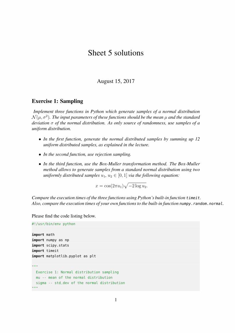
def sample_normal_twelve(mu, sigma):

""" Sample from a normal distribution using 12 uniform samples.

See lecture on probabilistic motion models slide 19 for details.

"""

# Formula returns sample from normal distribution with mean = 0

x = 0.5 * np.sum(np.random.uniform(-sigma, sigma, 12))

return mu + x

def sample_normal_rejection(mu, sigma):

"""Sample from a normal distribution using rejection sampling.

See lecture on probabilistic motion models slide 25 for details.

"""

# Length of interval from wich samples are drawn

interval = 5*sigma

# Maximum value of the pdf of the desired normal distribution

max_density = scipy.stats.norm(mu,sigma).pdf(mu)

# Rejection loop

while True:

x = np.random.uniform(mu - interval, mu + interval, 1)[0]

y = np.random.uniform(0, max_density, 1)

if y <= scipy.stats.norm(mu, sigma).pdf(x):

break

return x

def sample_normal_boxmuller(mu, sigma):

"""Sample from a normal distribution using Box-Muller method.

See exercise sheet on sampling and motion models.

"""

# Two uniform random variables

u = np.random.uniform(0, 1, 2)

# Box-Muller formula returns sample from STANDARD normal distribution

x = math.cos(2*np.pi*u[0]) * math.sqrt(-2*math.log(u[1]))

return mu + sigma * x

def evaluate_sampling_time(mu, sigma, n_samples, sample_function):

tic = timeit.default_timer()

for i in range(n_samples):

sample_function(mu, sigma)

toc = timeit.default_timer()

time_per_sample = (toc - tic) / n_samples * 1e6

print "%30s : %.3f us" % (sample_function.__name__, time_per_sample)

2

def evaluate_sampling_dist(mu, sigma, n_samples, sample_function):

n_bins = 100

samples = []

for i in range(n_samples):

samples.append(sample_function(mu, sigma))

print "%30s : mean = %.3f, std_dev = %.3f" % (

sample_function.__name__, np.mean(samples), np.std(samples))

plt.figure()

count, bins, ignored = plt.hist(samples, n_bins, normed=True)

plt.plot(bins, scipy.stats.norm(mu, sigma).pdf(bins), linewidth=2, color=’r’)

plt.xlim([mu - 5*sigma, mu + 5*sigma])

plt.title(sample_function.__name__)

def main():

mu, sigma = 0, 1

sample_functions = [

sample_normal_twelve,

sample_normal_rejection,

sample_normal_boxmuller,

np.random.normal

]

for fnc in sample_functions:

evaluate_sampling_time(mu, sigma, 1000, fnc)

n_samples = 10000

print "evaluting sample distances with:"

print " mean :", mu

print " std_dev :", sigma

print " samples :", n_samples

for fnc in sample_functions:

evaluate_sampling_dist(mu, sigma, n_samples, fnc)

plt.show()

if __name__ == "__main__":

main()

Exercise 2: Odometry-based Motion Model

A working motion model is a requirement for all Bayes Filter implementations. In thefollowing, you will implement the simple odometry-based motion model.

(a) Implement the odometry-based motion model in Python. Your function should take

3

the following three arguments

~xt =

xyθ

~ut =

δr1δr2δt

α =

α1

α2

α3

α4

,

where ~xt is the pose of the robot before moving, ~ut is the odometry reading obtainedfrom the robot, and α are the noise parameters of the motion model. The returnvalue of the function should be the new pose ~xt+1 of the robot predicted by themodel.

As we do not expect the odometry measurements to be perfect, you will have totake the measurement error into account when implementing your function. Usethe sampling methods you implemented in Exercise 1 to draw normally distributedrandom numbers for the noise in the motion model.

Please find the code listing below. The code assumes that the solution to exercise 1is stored as sample_normal_distribution.py.

(b) If you evaluate your motion model over and over again with the same startingposition, odometry reading, and noise values what is the result you would expect?

Each evaluation will give a different result. The three steps of the motion (rotation 1,translation, rotation 2) will be randomized according to the odometry model:

δ̂r1,2 = δr1,2 + normal(α1|δr1,2|+ α2δt) (1)

δ̂t = δt + normal(α3δt + α4(|δr1|+ |δr2|)) (2)

The pure rotational uncertainty is given by α1, while the pure translational uncer-tainty is given by α3. The translation affects both rotations through α2 and bothrotations affect the translation through α4. The most probable result is the onewithout noise (the robot moves exactly as given by ~ut).

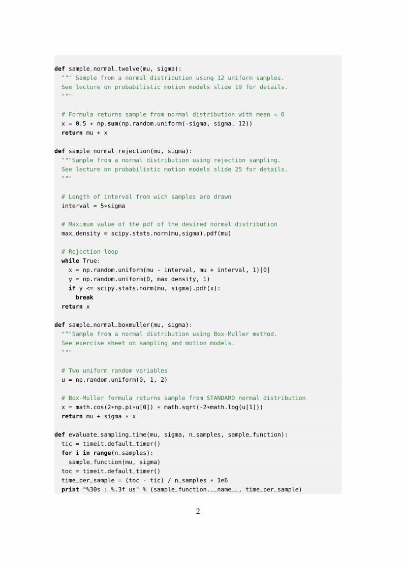
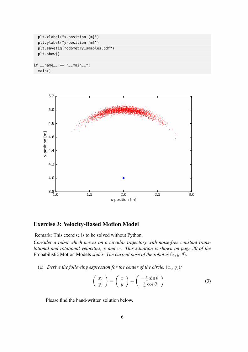
(c) Evaluate your motion model 5000 times for the following values

~xt =

2.04.00.0

~ut =

π2

0.01.0

α =

0.10.10.010.01

.

Plot the resulting (x, y) positions for each of the 5000 evaluations in a single plot.

Please find the code listing and figure below.

#!/usr/bin/env python

import sample_normal_distribution as snd

import numpy as np

import math

4

import matplotlib.pyplot as plt

""" Exercise 2 a) Implement odometry-based motion model """

def sample_normal(mu, sigma):

return snd.sample_normal_twelve(mu,sigma)

#return snd.sample_normal_rejection(mu,sigma)

#return snd.sample_normal_boxmuller(mu,sigma)

#return np.random.normal(mu,sigma)

def sample_odometry_motion_model(x, u, a):

""" Sample odometry motion model.

Arguments:

x -- pose of the robot before moving [x, y, theta]

u -- odometry reading obtained from the robot [rot1, rot2, trans]

a -- noise parameters of the motion model [a1, a2, a3, a4]

See lecture on probabilistic motion models slide 27 for details.

"""

delta_hat_r1 = u[0] + sample_normal(0, a[0]*abs(u[0]) + a[1]*u[2])

delta_hat_t = u[2] + sample_normal(0, a[2]*u[2] + a[3]*(abs(u[0])+abs(u[1])))

delta_hat_r2 = u[1] + sample_normal(0, a[0]*abs(u[1]) + a[1]*u[2])

x_prime = x[0] + delta_hat_t * math.cos(x[2] + delta_hat_r1)

y_prime = x[1] + delta_hat_t * math.sin(x[2] + delta_hat_r1)

theta_prime = x[2] + delta_hat_r1 + delta_hat_r2

return np.array([x_prime, y_prime, theta_prime])

""" Exercise 2 c) Evaluate motion model """

def main():

x = [2, 4, 0]

u = [np.pi/2, 0, 1]

a = [0.1, 0.1, 0.01, 0.01]

num_samples = 5000

x_prime = np.zeros([num_samples, 3])

for i in range(0, num_samples):

x_prime[i,:] = sample_odometry_motion_model(x,u,a)

plt.plot(x[0], x[1], "bo")

plt.plot(x_prime[:,0], x_prime[:,1], "r,")

plt.xlim([1, 3])

plt.axes().set_aspect(’equal’)

5

plt.xlabel("x-position [m]")

plt.ylabel("y-position [m]")

plt.savefig("odometry_samples.pdf")

plt.show()

if __name__ == "__main__":

main()

1.0 1.5 2.0 2.5 3.0x-position [m]

3.8

4.0

4.2

4.4

4.6

4.8

5.0

5.2

y-p

osi

tion [

m]

Exercise 3: Velocity-Based Motion Model

Remark: This exercise is to be solved without Python.Consider a robot which moves on a circular trajectory with noise-free constant trans-lational and rotational velocities, v and w. This situation is shown on page 30 of theProbabilistic Motion Models slides. The current pose of the robot is (x, y, θ).

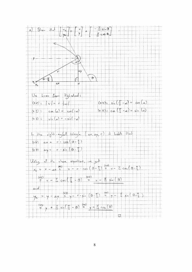
(a) Derive the following expression for the center of the circle, (xc, yc):(xcyc

)=

(xy

)+

(− vwsin θ

vwcos θ

)(3)

Please find the hand-written solution below.

6

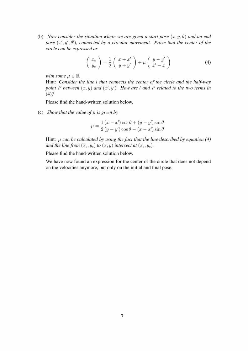
(b) Now consider the situation where we are given a start pose (x, y, θ) and an endpose (x′, y′, θ′), connected by a circular movement. Prove that the center of thecircle can be expressed as(

xcyc

)=

1

2

(x+ x′

y + y′

)+ µ

(y − y′x′ − x

)(4)

with some µ ∈ RHint: Consider the line l that connects the center of the circle and the half-waypoint P between (x, y) and (x′, y′). How are l and P related to the two terms in(4)?

Please find the hand-written solution below.

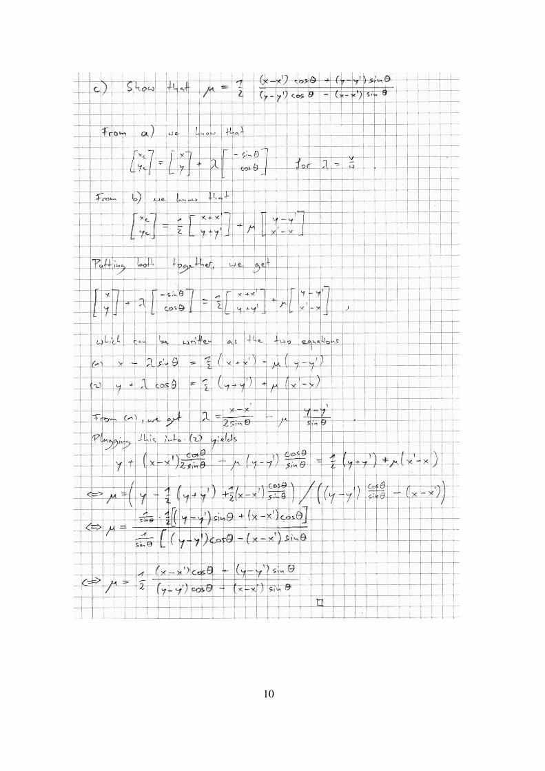
(c) Show that the value of µ is given by

µ =1

2

(x− x′) cos θ + (y − y′) sin θ(y − y′) cos θ − (x− x′) sin θ

.

Hint: µ can be calculated by using the fact that the line described by equation (4)and the line from (xc, yc) to (x, y) intersect at (xc, yc).

Please find the hand-written solution below.

We have now found an expression for the center of the circle that does not dependon the velocities anymore, but only on the initial and final pose.

7

8

Note: ~u is ~v rotated by 90◦, which can be shown using a 2D rotation matrix.

9

10