Shallow Water Flow through a Contraction

Benjamin Akers

Department of Mathematics, University of Wisconsin, U.S.A.

July 18, 2006

1 Introduction

Shallow water flows in channels are of interest in a variety of physical problems. Theseinclude river flow through a canyon, river deltas, and canals. Under certain conditions wecan get large hydraulic jumps, or their moving counterparts bores, in the channel. Thereare a number of places where these bores are generated in rivers around the world, includingthe River Severn in England, and the Amazon in Brazil [6].

Figure 1: A surfer riding a tidal bore on the Amazon.

In this work, we will be concerned with the effect that geometry and flow rate have onthe formation and stability of hydraulic jumps. The general setup is inspired by Al-Taraziet al. [2] and Baines and Whitehead [4]. The motivations are to use the present study toinvestigate shallow water flow and also as a tool for comparison with the granular mediaflows studied in [2]. The idea being that this will lay a foundation for the study of mixedmedia flows.

97

The body of this report is divided into five sections. First we will present the onedimensional inviscid hydraulic theory. Then we will compare the inviscid theory with theexperimental results. Next we will discuss some two dimensional and frictional effects.Finally, we will discuss some areas for future research and make some concluding remarks.

2 Experimental setup

We conducted a series of experiments in a linear flume with a flat bottom and piecewiselinear cross section. Water flows through a sluice gate at the beginning of our channel,pours out of the end into a large reservoir, and is recirculated using pumps. The setup isshown in Figure 2.

Figure 2: The experiments were done in a linear plexiglass flume, where water was recircu-lated using pumps in a large trash can, seen on the right, downstream of the contraction.

The flume had a 20 cm cross section, and was approximately 1.5 m in length. When allthree of the pumps were in operation, we could generate a volume flux up to 4 liters/sec. Foreach experiment two plexiglass paddles, 30.5 cm long, are fixed at a given angle at the end ofthe channel. The flow rate is set by turning on the desired number of pumps and restrictingthe flow until the various flow states are observed. The flow rate is then measured using abucket and a stopwatch at the end of the channel. In order to increase the accuracy of ourflow measurement, the discharge was measured a minimum of five times and the mean ofthese measurements was taken as the flow rate. In each experiment the height of the fluidis measured by placing a thin ruler in the fluid parallel to the flow velocity and visuallyestimating the depth. Data was taken at a variety of nozzle widths and flow speeds. Aschematic of the experimental setup is shown in Figure 3.

98

s l u i c e g a t e c o n t r a c t i o nxxxxxxxxxxxxxxxxxxxxxxxxxxxx

xxxxxxxxxxxxxxxxxxxxxxxxxxxxxxxxxxxxxxxxxxxxxxxxxxxxxxxxxxxxxxxxxxxxxxxxxxxxxxxxxxxx

xxxxxxxxxxxxxxxxxxxxxxxxxxxxxxx

xxxxxxxxxxxxxxxxxxxxxxxxxxxxxx

xxxxxxxxxxxxxxxxxxxxxxxxxxxxxxxxxxxxxxxxxxxxxxxxxxxxxxxxxxxxxxxxxxxxxxxxxxxxxxxxxxxxxxxxxxxxxxxxxxxxxxxx

xxxx

xxxxxxxxxxxx 2 0 c mSid eVi ew

T opVi ewxxxxxxxxxxxxxxxxxxxxxxxxxxxxxxxxxxxxxxxxxxxxxxxxxxxxxxxxxxxxxxxxxxxxx1 5 0 c m

a i r

Figure 3: A sketch of the tank is given. The tank is piecewise linear, with paddles at theend to regulate the nozzle width.

3 One Dimensional Inviscid Flows

Here we will present the mathematical formulation of the problem of flow through a channelwith a contraction. We will derive the governing equations from conservations laws and usethese to give predictions for steady one dimensional (1-D) flows. Next, we will determinethe necessary flow conditions for moving shocks, as well as for stationary shocks. Finally,we will derive a stability condition for steady shocks in a contraction.

3.1 Conservation Laws

Conservation of mass of a constant density fluid in a shallow channel can be written as

d

dt

∫ x1

x0

∫ b(x)

0

∫ h(x,y,t)

0ρdzdydx =

∫ b(x)

0

∫ h(x,y,t)

0ρ(

u(x0, y, t) − u(x1, y, t))

dzdy, (1)

where the x-axis is measured down the centerline of the channel, x0 and x1 are arbitrarypoints on this axis, and t is time. If we use the divergence theorem on the integral on theright hand side, and take h and u to be independent of y this becomes

∫ x1

x0

[ρb(x)h(x, t)]t + [ρb(x)h(x, t)u(x, t)]x dx = 0. (2)

Since x0 and x1 are arbitrary we get that the argument of our integral must be equal zeropointwise

(bh)t + (bhu)x = 0. (3)

Here u is the velocity, h the height of the free surface, b the width of the channel, and ρ thedensity of the fluid. Partial derivatives are written in two ways as ∂t(·) = (·)t and so forth.

99

For water, ρ, is taken constant, and we therefore have dropped the ρ dependence from (3).We can also get a momentum equation using Newton’s second law of motion

d

dt

∫

CVρu(x, y, t)dV =

∫

CSρu(x, y, t)2 · ndA +

∫

CVFdV +

∫

CSS · ndA, (4)

where dA and dV are infinitesimal area and volume elements. To make the notation simplerwe have omitted the bounds of our integrals, instead writing CV for an arbitrary controlvolume, and CS for the surface of that volume. If we make the assumption that the pressureforces are hydrostatic, then the acceleration in the vertical direction is negligible, and thebody forces must balance the surface stress to give hydrostatic pressure p− p0 = ρg(h − y)(see, e.g., [9]), where g is the acceleration due to gravity. We can use Stokes’ theorem toturn (4) into a volume integral, and after assuming again h = h(x, t), u = u(x, t) we obtain

(bhu)t + (bhu2)x +1

2gb(h2)x = 0. (5)

3.2 Smooth Hydraulic Flow

In this section, we are looking at flows which have reached a steady state. This allows usto simplify (3) and (5) into

(bhu)x = 0 (6a)

(bhu2)x +1

2gb(h2)x = 0. (6b)

When the solutions are smooth we can expand the derivatives in (6b) to get

(1

2u2 + gh)x = 0. (7)

Next, introduce the local Froude number, F = u/√

gh. Eliminating ux from (6) yields

−u2

gh(bh)x + bhx = 0 (8)

or(1 − F 2)bhx = F 2hbx. (9)

Thus we see that if F = 1 then b must be stationary, or in our case at a minimum. Notethat the converse is not true, when bx = 0 we have that F = 1 or hx = 0 but not necessarilyboth. We will define the flow to be subcritical when F < 1 and supercritical when F > 1.Equation (9) tells us that for smoothly contracting b(x), the subcritical fluid flow must havea minimum in h at the nozzle. Similarly, supercritical flow must have a maximum at thenozzle, see Figure 4.

Next we will examine for what range of far field Froude numbers F0 = u0/√

gh0 andcontraction ratios B = bc/b0, we can have smooth solutions. Since the flow is smooth wecan follow the two constants of the flow

Q = b0h0u0 = bchcuc (10a)

E = u20/2 + gh0 = u2

c/2 + ghc. (10b)

100

xxxxxxxxxxxxxxxxxxxxxxxxxxxxxxxxxxxxxxxxxxxxxxxxxxxxxxxxxxxxxxxx

S u p e r c r i t i c a l F l o wT o p v i e wS i d e v i e w

xxxxxxxxxxxxxxxxxxxxxxxxxxxxxxxxxxxxxxxxxxxxxxxxxxxxxxxxxxxxxxxx

S u p e r c r i t i c a l F l o wT o p v i e wS i d e v i e w

xxxxxxxxxxxxxxxxxxxxxxxxxxxxxxxxxxxxxxxxxxxxxxxxxxxxxxxxxxxxxxxxxxxx

S u b c r i t i c a l F l o wFigure 4: The shape of the free surface of supercritical and subcritical smooth flow througha nozzle. Both the top view and a profile are shown in this figure.

If we non-dimensionalize, H = hc/h0 and B = bc/b0, then (10) is equivalent to the cubicpolynomial, p(H) = 0, with parameters B and F0, where

P (H) = H3B2 − (1

2F 2

0 + 1)B2H2 +1

2F 2

0 = 0. (11)

0.1 0.2 0.3 0.4 0.5 0.6 0.7 0.8 0.9 1 1.1

0.5

1

1.5

2

2.5

3

3.5

4

4.5

F0

Bc

Smooth Flows

No Smooth Flows

Figure 5: The smooth solution boundary is plotted in the BcF0-plane, where Bc is thenondimensional contraction width, and F0 is the ratio of the flow speed to the characteristicflow rate of the fluid. We note that Bc = 1 corresponds to a blocked flow and Bc = 1corresponds to a straight channel.

The stationary points of this cubic are at H = 0 and H∗ = 23(1

2F 20 + 1). Now since

physically meaningful roots exist only for H > 0, we can determine when there are positiveroots by evaluating P (H) at H = H∗. When p(H∗) <= 0 there are positive roots, andwhen p(H∗) > 0 there are no positive roots. Thus the point p(H∗) = 0 determines the

101

boundary between smooth and nonsmooth solutions in the BcF0-plane. This is a standardtechnique in hydraulic theory [7]. We obtain

3

2

(

F0

Bc

)2/3

− (1 +1

2F 2

0 ) = 0. (12)

Figure 5 illustrates how for a given geometry Bc and incoming depth h0 there is a maximumspeed at which a subcritical smooth flow can pass. It is also interesting to note that forchannels with expanding width B > 1 we can find a smooth flow regardless of the speed.In the next section we will look at non-smooth flows.

3.3 Upstream Moving Bores

Here we will look for solutions with a discontinuity, or jump, at one point. We will allowthis jump to move upstream at speed s, where s is positive when moving to the left, as inFigure 6.

xxxxxxxxxxxxxxxxxxxxxxxxxxxxxxxxxxxxxxxxxxxxxxxxxxxxxxxxxxxxxxxxxxxxxxxxxxxxxxxxxxxxxxxxxxxxxxxxxxxxxxxxxxxxxxxxxxxxxxxxxxxxxxxxxxxxxxxxxxxxxxxxxxxxxxxxxxxxxxxxxxxxxxxxxxxxxxxxxxxxxxxxxxxxxxxxxxxxxxxxxxxxxxxx

xxxxxxxxxxxxxxxxxxxxxxxxxxxxxxxxxxxxxxxxxxxxxxxxxxxxxxxxxxxxxxxxxxxxxxxxxxxxxxxxxxxxxxxxxxxxxxxxxxxxxxxxxxxxxxxxxxxxxxxxxxxxxxxxxxxxxxxxxxxxxxxxxxxxxxxxxxxxxxxxxxxxxxxxxxxxxxxxxxxxxxxxxxxxxxxxxxxxxxxxxxxxx 0 x 1 x c

h 0u 0b 0 h 1u 1b 0 h cu cb cs x T o p v i e wS i d e v i e wFigure 6: Both the free surface profile and the planar view are shown. Here we have a shockmoving upstream with speed s. Conservation laws will be used to couple the fluid motionbetween points x0, x1, and xc.

As in Figure 6, we will pick a point upstream, x0, one between the jump and the nozzle,x1, and the point of minimum width at the nozzle, xC . We will label the width, height,and velocity at these points with subscripts that match the respective points. The goal isto find in which regions of the BcF0-plane there exist shock solutions. We can couple theflow at points x1 and xC using Bernoulli’s equation (13c) and conservation of mass (13b) asbefore. The flow at points x0 and x1 can be coupled by conservation of mass in the frameof the jump (13a) and a jump condition (13d) which we can derive from the conservativeform of the momentum equation. Consequently, we have four equations for five unknowns,

102

so we impose the restriction that flow is critical (13e) at the nozzle, and obtain the system

(u0 + s)h0b0 = (u1 + s)h1b1 (13a)

u1h1b1 = uchcbc (13b)

1

2u2

1 + gh1 =1

2u2

c + ghc (13c)

(u0 + s)2 =gh1

2(1 +

h1

h0) (13d)

u2c = ghc. (13e)

Taking a critical condition at the nozzle is a common assumption in hydraulics. It isequivalent to imposing the restriction that there are no waves at infinity [5]. Now, we have asystem of five equations for five unknowns u1, uc, hc, h1, s, with parameters h0, u0, b1 = b0, bc.Nondimensionalizing B = bc/b0, F0 = u0/

√gh0,H1 = h1/h0, S = s/

√gh0, system (13)

simplifies to

1

2(F0 + (1 − H1)S)2 =

3

2H2

1

(

F0 + (1 − H1)S

Bc

)2/3

− H31 (14a)

(F0 + S)2 =1

2H1(1 + H1). (14b)

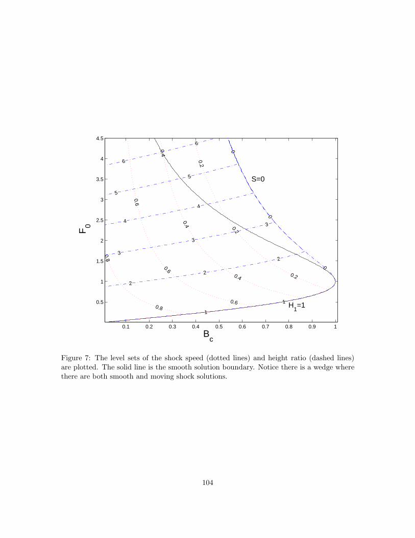
Figure 7 shows the region of the BcF0-plane where (14) has physically meaningful solutions.This region was obtained by first fixing H1 and then finding the solution curves for S andthen fixing S and finding the solution curves for H1. The boundaries correspond to smoothflow H1 = 1 and steady shocks S = 0.

103

0.1 0.2 0.3 0.4 0.5 0.6 0.7 0.8 0.9 1

0.5

1

1.5

2

2.5

3

3.5

4

4.5

Bc

F0

1

0

0

0

0.2

0.2

0.2

0.4

0.4

0.4

0.6

0.6

0.6

0.80.8

1

2

2

2

3

3

3

4

4

5

5

6

6

S=0

H1=1

Figure 7: The level sets of the shock speed (dotted lines) and height ratio (dashed lines)are plotted. The solid line is the smooth solution boundary. Notice there is a wedge wherethere are both smooth and moving shock solutions.

104

3.4 Hydraulic Jumps in the Contraction

Here we examine for which flow rates F0 and contraction widths Bc there can be steadyshocks. Steady shocks in a contraction are solutions to

u0h0b0 = u1h1b1 = u2h2b1 = uchcbc (15a)

1

2u2

0 + gh0 =1

2u2

1 + gh1 (15b)

1

2u2

2 + gh2 =1

2u2

c + ghc (15c)

u21 =

gh2

2(1 +

h2

h1) (15d)

u2c = ghc. (15e)

These seven equations are mass and momentum balance between four locations plus thecritical condition. The four locations are the far upstream, h0, u0, b0, the upstream limitof the shock u1, h1, b1, the downstream limit h2, u2, b1, and the nozzle uc, hc, bc. If wenondimensionalize as follows, H1 = h1/h0, H2 = h2/h0, Bc = bc/b0, then we can reduce(15) to

1

4H2

2 − (1

2F 2

0 + 1)H1 +1

4H1H2 + H2

1 = 0 (16a)

H22 −

3

2(F0

Bc)2/3H2 +

1

4H1H2 +

1

4H2

1 = 0. (16b)

We will use (16) to find where in the F0B-plane we have steady shocks. A simple way to dothis is to consider what the boundaries of this region should be. If we have a shock we knowfrom the energy condition that H1 ≤ H2 [3]. Now if we look at where this upper bound onH1 is satisfied with equality H1 = H2, we can then reduce (16) to

1

2F 2

0 + 1 −3

2(F0

Bc)2/3 = 0, (17)

which is the boundary (12) of smooth solutions we already determined. This boundarycame from considering an upper bound on H1. The other boundary should then come froma lower bound. Since we are working here with supercritical flow in a contracting region,we expect H1 to grow the farther we move into the contraction. Thus the other boundaryshould be when the shock is at the mouth of the contraction, or when H1 = 1. Substitutingthis into equations (16a) and (16b) yields

5 + 16F 20 + 6(

F0

Bc)2/3 − 3

√

1 + 8F 20 − 6(

F0

Bc)2/3

√

1 + 8F 20 = 0. (18)

This is the limiting curve we found for moving shocks when the speed goes to zero. Thuswe have steady shocks in the contraction only in the wedge of Figure 7 where we had bothsmooth solutions and upstream moving shocks.

Next we examine the stability of steady shocks. Consider a system with a steady shockin the contraction region, with u1 and h1 the upstream limit of the velocity and height at

105

xxxxxxxxxxxxxxxxxxxxxxxxxxxxxxxxxxxxxxxxxxxxxxxxxxxxxxxxxxxxxxxxxxxxxxxxxxxxxxxxxxxxxxxxxxxxxxxxxxxxxxxxxxxxxxxxxxxxxxxxxxxxxxxxxxxxxxxxxxxxxxxxxxxxxxxxxxxxxxxxxxxxxxxxxxxxxxxxxxxxxxxxxxxxxxxxxxxxxxxxxxxx

xxxxxxxxxxxxxxxxxxxxxxxxxxxxxxxxxxxxxxxxxxxxxxxxxxxxxxxxxxxxxxxxxxxxxxxxxxxxxxxxxxxxxxxxxxxxxxxxxxxxxxxxxxxxxxxxxxxxxxxxxxxxxxxxxxxxxxxxxxxxxxxxxxx

h 2h 1 h 2 + hε2

h 1 + hε1

Figure 8: Sketch of the unperturbed solution (solid curve) juxtaposed over the perturbedshock (dashed curve).

the shock and u2, h2 the downstream limit. Now we will assume a small perturbation whichgenerates a shock moving at a small speed s, see Figure 3.4.

Let us present equations which govern the perturbed flow. The perturbations are de-noted with a superscript ǫ. The perturbed flow balances mass and momentum over theshock

(u1 + uǫ1 + s)(h1 + hǫ

1) = (u2 + uǫ2 + s)(h2 + hǫ

2) (19)

(u1 + uǫ1 + s)2(h1 + hǫ

1) +g

2(h1 + hǫ

1)2 = (u2 + uǫ

2 + s)2(h2 + hǫ2) +

g

2(h2 + hǫ

2)2.(20)

Mass will be conserved upstream of the jump

(u1 + uǫ1)(b + bǫ)(h1 + hǫ

1) = Q. (21)

We will assume that the perturbation does not affect the far field momentum upstream E1

or downstream E2, so the Bernoulli constants are unchanged

1

2(u1 + uǫ

1)2 + g(h1 + hǫ

1) = E1 =1

2u2

1 + gh1 (22)

1

2(u2 + uǫ

2)2 + g(h2 + hǫ

2) = E2 =1

2u2

2 + gh2. (23)

Now we assume that we have a small perturbation and small resulting shock speed. Lin-earizing all these equations gives a linear system of six unknowns and five equations

uǫ1h1b + u1h1b

ǫ + u1bhǫ1 = 0 (24a)

uǫ1h1 + sh1 + u1h

ǫ1 − uǫ

2h2 − sh2 − u2hǫ2 = 0 (24b)

2h1u1(uǫ1 + s) + hǫ

1u21 + gh1h

ǫ1 − 2h2u2(u

ǫ2 + s) − hǫ

2u22 − gh2h

ǫ2 = 0 (24c)

u1uǫ1 + ghǫ

1 = 0 (24d)

u2uǫ2 + ghǫ

2 = 0. (24e)

The goal is to reduce this to a single equation for the perturbed shock speed s in terms ofthe change in channel width bǫ. If bǫ and s have opposite signs and we are in a contraction,then the solution is stable, because the shock speed will force the shock back to its previous

106

xxxxxxxxxxxxxxxxxxxxxxxxxxxxxxxxxxxxxxxxxxxxxxxxxxxxxxxxxxxxxxxxxxxxxxxxxxxxxxxxxxxxxxxxxxxxxxxxxxxxxxxxxxxxxxxxxxxxxxxxxxxxxxxxxxxxxxxxxxxxxxxxxxxxxxxxxxxxxxxxxxxxxxxxxxxxxxxxxxxxxxxxxxxxxxxxxxxxxxxxxxxxxxxxxxxxxxxxxxxxxxxxxxxxxxxxxxxxxxxxxxxxxxxxxxxxxxxxxxxxxxxxxxxxxxxxxxxxxxxxxxxxxxxxxxxxxxxxxxxxxxxxxxxxxxxxxxxxxxxxxxxxxxxxxxxxxxxxxxxxxxxxxxxxxxxxxxxxxxxxxxxxxxxxxxxxxxxxxxxxxxxxxxxxxxxxxxxxxxxxxxxxxxxxxxxxxxxxxxxxxxxxxxxxxxxxxxxxxxxxxxxxxxxxxxxxxxxxxxxxxxxxxxxxxxxxxxxxxxxxxxxxxxxxxxxxxxxxxxxxxxxxxxxxxxxxxxxxxxxxxxxxxxxxxxxxxxxxxxxxxxxxxxxxxxxxxxxxxxxxxxxxxxxxxxxxxxxxxxxxxxxxxxxxxxxxxxxxxxxxxxxxxxxxxxxxxxxxxxxxxxxxxxxxxxxxxxxxxxxxxxxxxxxxxxxxxxxxxxxxxxxxxxxxxxxxxxxxxxxxxxxxxxxxxxxxxxxxxxxxxxxxxxxxxxxxxxxxxxxxxxxxxxxxxxxx

xxxxxxxxxxxxxxxxxxxxxxxxxxxxxxxxxxxxxxxxxxxxxxxxxxxxxxxxxxxxxxxxxxxxxxxxxxxxxxxxxxxxxxxxxxxxxxxxxxxxxxxxxxxxxxxxxxxxxxxxxxxxxxxxxxxxxxxxxxxxxxxxxxxxxxxxxxxxxxxxxxxxxxxxxxxxxxxxxxxxxxxxxxxxxxxxxxxxxxxxxxxxxxxxxxxxxxxxxxxxxxxxxxxxxxxxxxxxxxxxxxxxxxxxxxxxxxxxxxxxxxxxxxxxxxxxxxxxxxxxxxxxxxxxxxxxxxxxxxxxxxxxxxxxxxxxxxxxxxxxxxxxxxxxxxxxxxxxxxxxxxxxxxxxxxxxxxxxxxxxxxxxxxxxxxxxxxxxxxxxxxxxxxxxxxxxxxxxxxxxxxxxxxxxxxxxxxxxxxxxxxxxxxxxxxxxxxxxxxxxxxxxxxxxxxxxxxxxxxxxxxxxxxxxxxxxxxxxxxxxxxxxxxxxxxxxxxxxxxxxxxxxxxxxxxxxxxxxxxxxxxxxxxxxxxxxxxxxxxxxxxxxxxxxxxxxxxxxxxxxxxxxxxxxxxxxxxxxxxxxxxxxxxxxxxxxxxxxxxxxxxxxxxxxxxxxxxxxxxxxxxxxxxxxxxxxxxxxxxxxxxxxxxxxxxxxxxxxxxxxxxxxxxxxxxxxxxxxxxxxxxxxxxxxxxxxxxxxxxxxxxxxxxxxxxxxxxxxxxxxxxxxxxxxxxxx

xxxxxxxxxxxxxxxxxxxxxx

xxxxxxxxxxxxxxxxxxxxxxxxxxxx

xxxx

xxxxxxxxxxxxxxxxx

xxxx

xxxxxxxxxxxxxxxx

xxx

xxxxxxxxxxxxxxxxxxxxxxxx

xxxx

xxxxxxxxxxxxxxxxxxx

S t a b l eU n s t a b l eb ( x )

xFigure 9: A sketch of the contraction region as viewed from above. The solid vertical linesdenote shocks. In a contracting region steady shocks are unstable, while in a dilation theyare stable.

position. If instead they have the same sign, then it is unstable, because the shock willpropagate away from its previous location, as shown in Figure 9.

After some algebra we obtain the relationship

S =F1(1 − u1

u2)

(1 − h2

h1)

Bǫ. (25)

Here S = s/√

gh1 and Bǫ = bǫ/b0. We know that across a physical shock, h2 > h1 andalso that u2 < u1, so this gives that sign(S)=sign(Bǫ). Details of the above calculation arefound in an appendix to this work [1].

4 Results

Experiments were conducted over a variety of flow speeds and channel geometries. In eachexperiment, the contraction width Bc was set and then the flow rate Q was varied. Theinflow height was kept fixed for all experiments at h0 = 1.3cm. The upstream channelwidth was also a constant b0 = 20cm. For each flow rate we recorded the category of theflow, either smooth flow, moving shock, steady shock, or oblique shock. These flow stateare depicted in Figure 10. For moving shocks the speed and height ratios across the shockwere measured. There is an experimental difficulty, in that we cannot measure the speed offast moving shocks. When measuring a flow, there is a time delay between when we initiatethe flow and when it reaches a steady state. In this experiment the time delay is on theorder of five seconds. Thus for flows with shock speeds larger than 15 cm/sec, the shockwill move to the end of our channel before we can properly measure the speed. The datafor the moving shocks where we could measure both the speed and the height are found inTable 1.

In addition to measuring the speed of moving shocks, we also took measurements whenwe had oblique shocks in the flow. Oblique shocks are a stationary phenomena in our flow,

107

xxxxxxxxxxxxxxxxxxxxxxxxxxxxxxxxxxxxxxxxxxxxxxxxxxxxxxxxxxxxxxxxxxxxxxxxxxxxxxxx

xxxx

xxxxxxxxxxxxxxxxxxxxxxxxxxxxxxxxxxxxxxxxxxxxxxxxxxxxxxxxxxxxxxxxxxxxxxxxxxxxxxxxxxxxx

xxxxxxxxxxxxxxxxxxxxxxxxxxxxxxxxxxxxxxxxxxxxxxxxxxxxxxxxxxxxxxxxxxxxxxxxxxxxxxxxxxxxx

xxxxxxxxxxxxxxxxxxxxxxxxxxxxxxxxxxxxxxxxxxxxxxxxxxxxxxxxxxxxxxxxxxxxxxxxxxxxxxxx

S m o o t h F l o w M o v i n g S h o c kS t e a d y S h o c k O b l i q u e S h o c k T o p v i e wS i d e v i e w

θc

θsFigure 10: Shown are sketches of the four types of flow behavior. Each sketch shows aprofile of the flow and a planar view.

Bc = bc/b0 F0 = u0/√

gh0 H1 = h1/h0 S = s/√

gh0

0.6 3.19 3.54 0.150.6 3.55 3.77 0.080.7 2.31 2.54 0.110.7 2.40 2.85 0.190.7 2.49 2.69 0.050.7 2.80 3.08 0.080.7 2.98 3.23 0.020.8 2.10 2.31 0.080.81 2.20 2.62 0.090.875 2.07 2.23 0.06

Table 1: The experimental data for moving shocks are presented here. Bc is the nondimen-sional contraction ratio; F0 the upstream Froude number; H1 the nondimensional heightratio across the shock; and S the nondimensional shock speed.

108

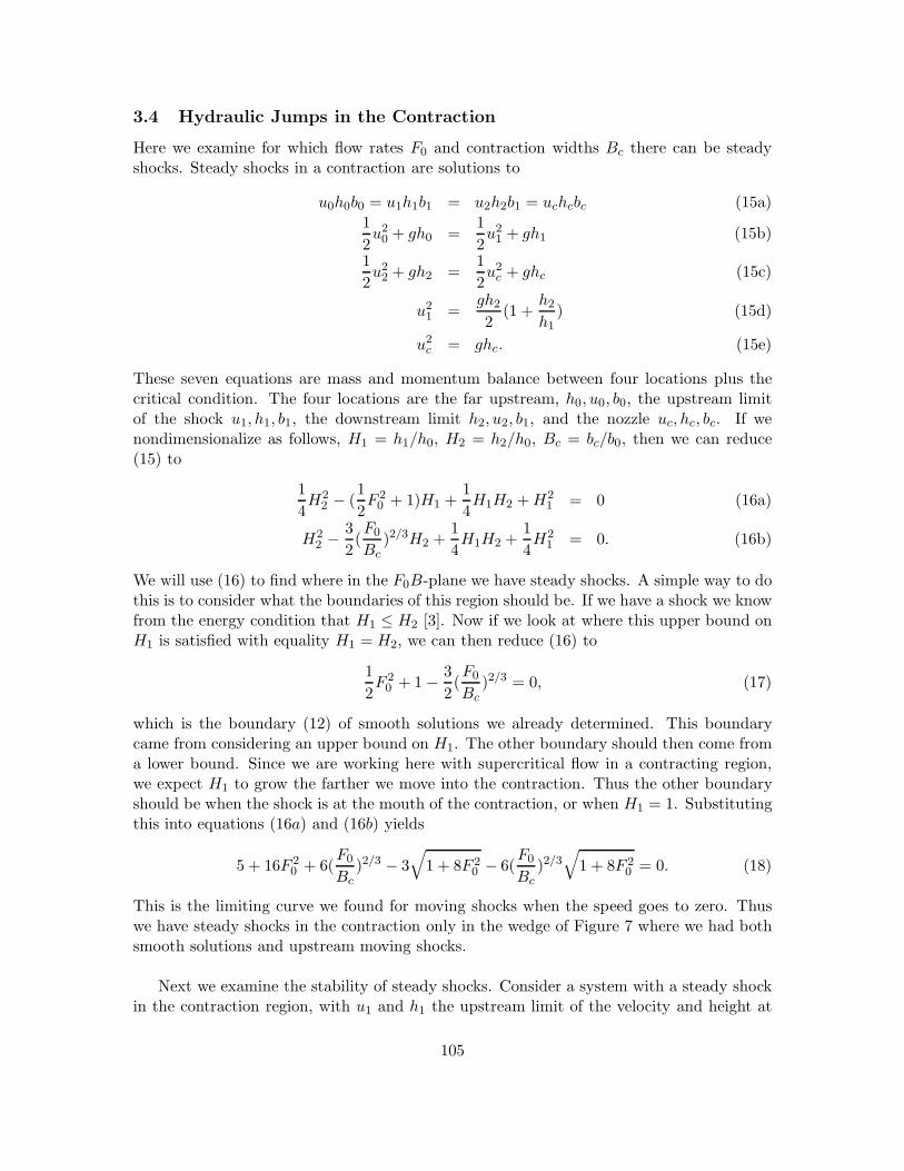
so we do not have the difficulty of measuring speed as in the moving case. There is a newdifficulty. When oblique shocks are very weak, surface tension effects will become impor-tant, and rather than a shock, we see capillary waves in our contraction region. A pictureof this phenomena is shown in Figure 11.

Figure 11: Weak shocks can be distorted by capillary waves.

Since we only want to measure oblique shocks, we need a criterion to determine whenwe have an oblique shock and when we have capillary waves. The criteria used here is thatwhen there is a measurable height difference between the fluid upstream and downstreamof the front, we call it an oblique shock. When the mean fluid height is the same on bothside of the front we call it a capillary wave. The data from the oblique shocks we measuredare presented in Table 2.

H1 = h1/h0 F0 = u0/√

gh0 θc θs

1.9 2.79 9.5 26.71.5 2.94 3.8 26.71.7 3.13 9.5 27.11.5 3.32 3.8 21.61.5 3.37 5.7 22.11.9 3.47 7.6 25.41.7 3.56 9.5 20.11.8 3.65 7.6 25.2

Table 2: The experimentally measured flow variables for the oblique shocks are presentedhere. H1 is the nondimensionalized height ratio across the shock, F0 is the upstream Froudenumber, θc is the angle of the contraction, θs is the angle of the shock, see also Figure 10.

109

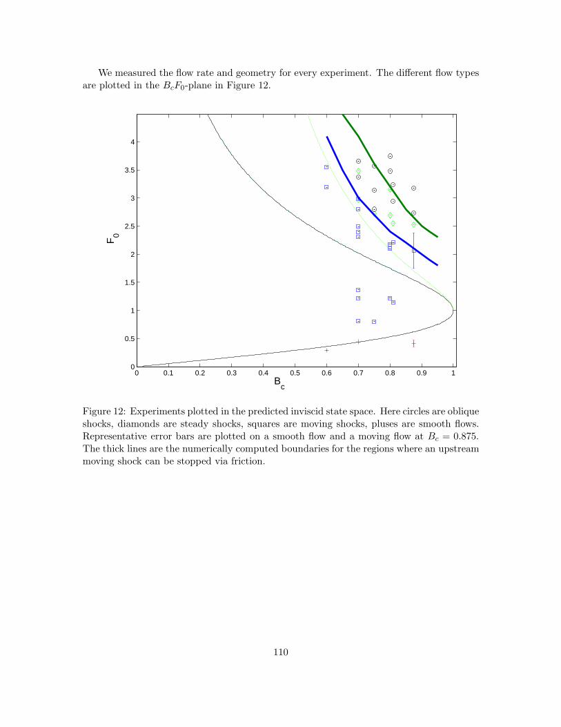
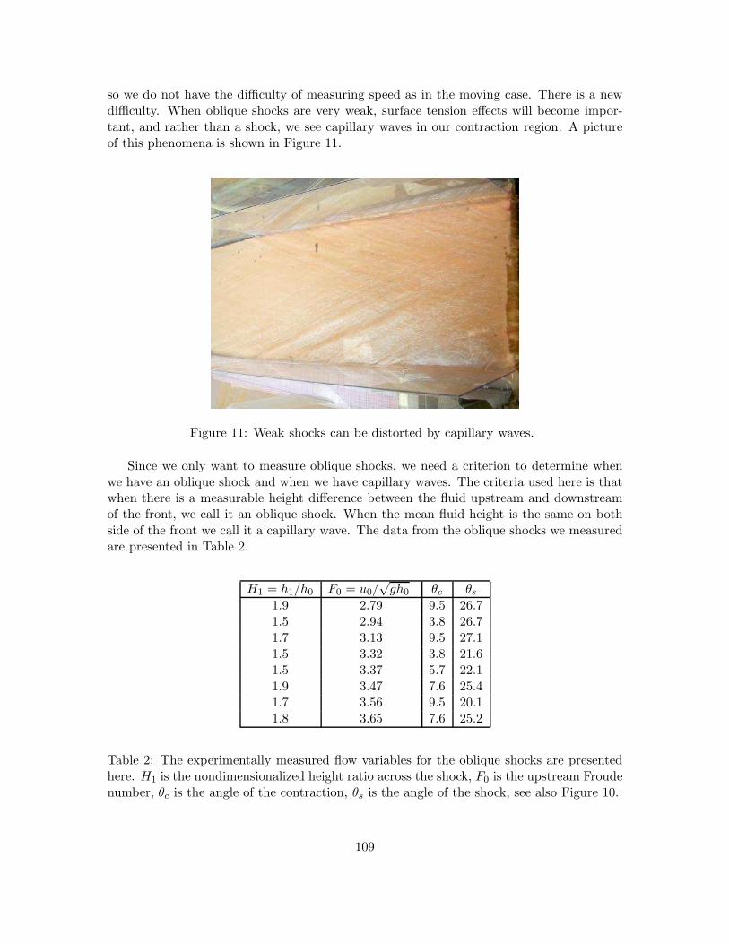
We measured the flow rate and geometry for every experiment. The different flow typesare plotted in the BcF0-plane in Figure 12.

0 0.1 0.2 0.3 0.4 0.5 0.6 0.7 0.8 0.9 10

0.5

1

1.5

2

2.5

3

3.5

4

Bc

F0

Figure 12: Experiments plotted in the predicted inviscid state space. Here circles are obliqueshocks, diamonds are steady shocks, squares are moving shocks, pluses are smooth flows.Representative error bars are plotted on a smooth flow and a moving flow at Bc = 0.875.The thick lines are the numerically computed boundaries for the regions where an upstreammoving shock can be stopped via friction.

110

5 Discussion

In this section we will compare the experimental results to mathematical theory. The modelsused in this report assume no effects of surface tension or viscosity. The importance ofthese effects are commonly measured using nondimensional numbers, Weber We for surfacetension and Reynolds Re for viscosity. Table 3 shows the range for these parameters in theexperiments considered.

Parameter Min Max

Reynolds (Re = UL/ν) 1,300 20,100Weber (We = ρU2L/σ) 1.85 433Froude (F0 = U0/

√gh0) 0.28 4.34

Contraction (Bc = bc/b0) 0.6 0.875

Table 3: The nondimensional parameters are estimated for the main body of our flow. HereWe ≈ 14F 2

0 and Re ≈ 3300F0. If we look at some local phenomena, for instance near weakoblique shocks, we can have smaller Weber and Reynolds numbers.

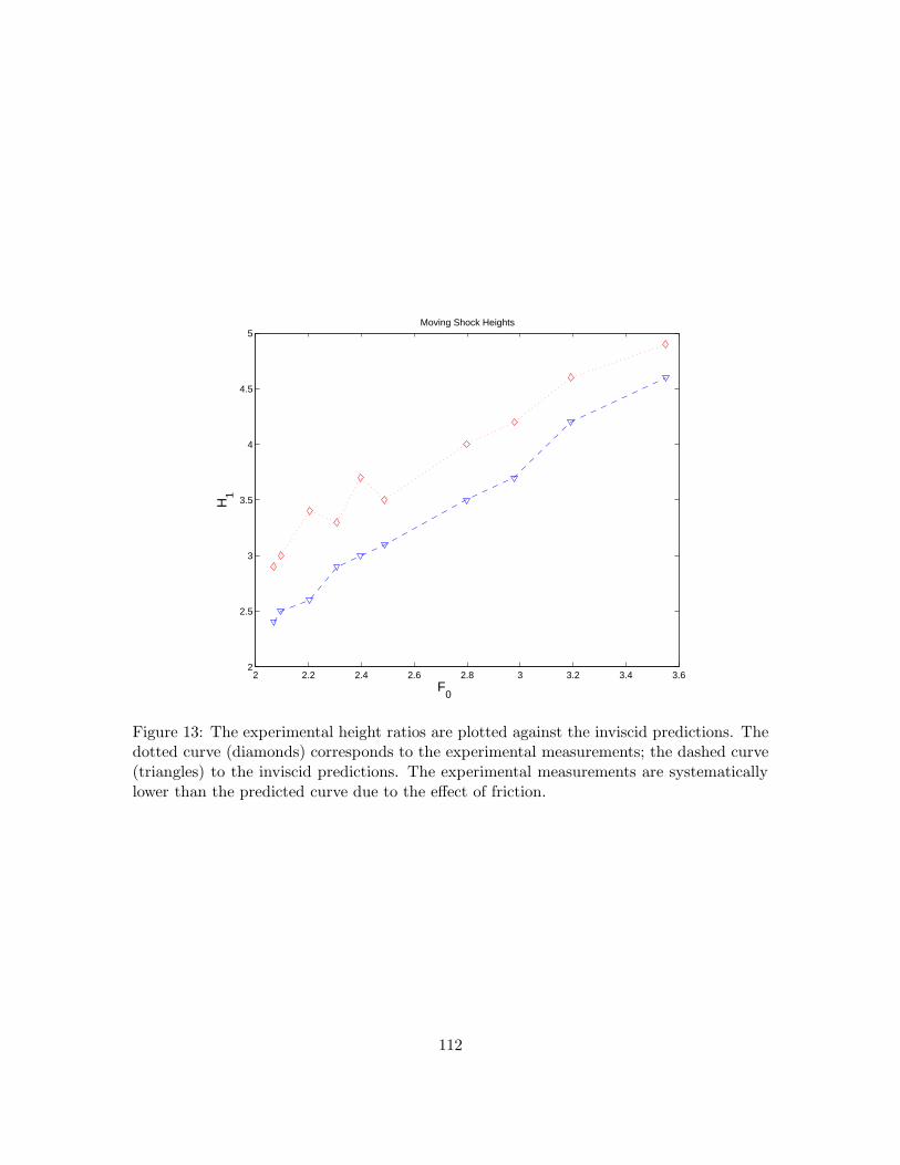
If we look at Equation (14) we see that for a given upstream Froude number F0 andnondimensional shock speed S, we can predict the height ratio across the shock. We can thencompare this prediction to the measured height ratios across the jump. This comparison isshown in Figure 13.

5.1 Oblique Shocks

All the analysis at the beginning of this report considered only 1-D phenomena. Obliqueshocks are a two-dimensional (2-D) phenomena, so our model does not take them intoaccount. Following [2] and [8], we can derive a system of equations for the oblique shockangle θs and shock height h1. These equations will allow us to predict θs and h1 given theupstream conditions h0, F0 and the angle of the contraction θc, as follows

h1

h0=

tan θs

tan(θs − θc)(26a)

sin θs =

√

1

2F 20

h1

h0(1 +

h1

h0). (26b)

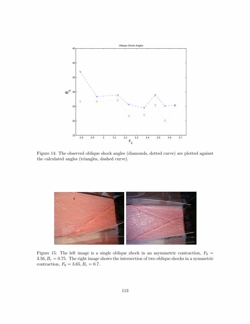
Using (26) we can plot our predicted oblique shock angles against the experimental ones.This plot is shown in Figure 14.

In our experiments we saw oblique shocks that exit our channel before interacting withanother shock, and oblique shocks that intersect in the channel, see Figure 15. A similarcalculation was also done which can be used to predict the angles of intersecting obliqueshocks.

111

2 2.2 2.4 2.6 2.8 3 3.2 3.4 3.62

2.5

3

3.5

4

4.5

5

F0

H1

Moving Shock Heights

Figure 13: The experimental height ratios are plotted against the inviscid predictions. Thedotted curve (diamonds) corresponds to the experimental measurements; the dashed curve(triangles) to the inviscid predictions. The experimental measurements are systematicallylower than the predicted curve due to the effect of friction.

112

2.8 2.9 3 3.1 3.2 3.3 3.4 3.5 3.6 3.715

20

25

30

35

40

45

F0

θ s

Oblique Shock Angles

Figure 14: The observed oblique shock angles (diamonds, dotted curve) are plotted againstthe calculated angles (triangles, dashed curve).

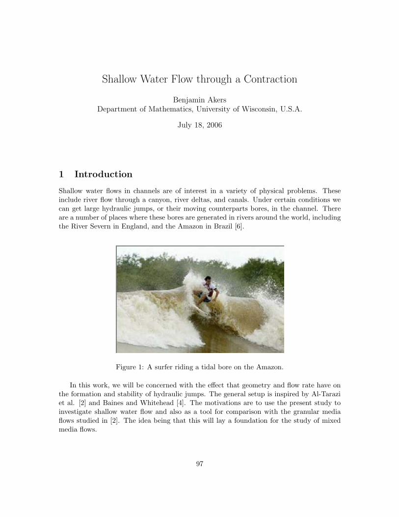
Figure 15: The left image is a single oblique shock in an asymmetric contraction, F0 =3.56, Bc = 0.75. The right image shows the intersection of two oblique shocks in a symmetriccontraction, F0 = 3.65, Bc = 0.7.

113

5.2 Turbulent Drag

If we examine Figure 12 we see that there are steady shocks outside of the region predictedby the inviscid theory. To explain this, we must reexamine the assumptions of the originalmodel. The real fluid does have some viscosity, so we should take this into account. In thehydraulic equations, viscous effects are usually added with a drag term. The most physicaldrag term comes from a quadratic drag law [3]. Adding such a term changes the hydraulicequations (6) to the system

uux + ghx = −Cdu2/h (27a)

(buh)x = 0. (27b)

This system of ordinary differential equations (ODE’s) can now be solved using standardnumerical techniques. When we do not have smooth solutions we can find steady shocksby using the inflow conditions at the sluice gate and critical condition at the nozzle asboundary conditions to march the solutions together until they match with a shock.

xxxxxxxxxxxxxxxxxxxxxxxxxxxxxxxxxxxxxxxxxxxxxxxxxxxxxxxxxxxxxxxxxxxx1 5 0 c m xxxxxxxxxxxxxxxxxxxxxxxxxxxxxxxxxxxxxxxxxxxxxxxxxxxxxxxx

F 0 F c = 1

Figure 16: A cartoon of the numerical method for finding steady shocks. We use an ODEsolver to find the smooth flow with a prescribed upstream Froude number F0 and the smoothflow that meets the critical condition Fc = 1. These two smooth flows are then matchedusing the shock condition.

Depending on the Froude number F0 and geometry Bc, we may or may not be able tohave a steady shock of this type. If we solve this system throughout our state space we getnumerically computed boundaries for when we can have steady shocks with friction. Theseboundaries are plotted in Figure 12. For our computations we have used Cd = 0.004 [4].

5.3 Multiple States

In our inviscid calculations, we predicted a region in the BcF0-plane where we can havethree different steady states: steady shocks, moving shocks, and supercritical smooth flows.We have shown that the steady shocks in the contraction region are unstable, so we don’texpect to see these. We also have observed that friction can stop slowly moving shocks, andthat supercritical smooth flows correspond to oblique shocks. Thus this region of multiplestates really corresponds to flow speeds where we can have upstream steady shocks, stopped

114

via friction, and oblique shocks in the contraction region. These phenomena were observedin the lab. Figure 12 shows both oblique shocks and steady shocks in the same region ofstate space. We also observed that large perturbations of these flows can cause the flowto change from one steady state to another. If we have a steady upstream shock, we canphysically push most of the water that is behind the shock out of the channel, and see asteady oblique shock. If we have an oblique shock, we can block the flow for a small timeperiod, and the resulting flow will evolve into a steady upstream shock. Figure 17 showssnapshots of the transition from oblique shocks to an upstream steady shock.

Figure 17: Shown are snapshots of the flow transition from oblique shocks to a steadyupstream shock. The time interval between each frame is 1 second. Here we have theFroude number F0 = 2.8 and the contraction ratio Bc = 0.7. A ruler is used to restrict theflow for a small time period to induce this state change.

6 Conclusion and future work

We presented a mathematical and experimental investigation into shallow water flow througha contraction. We began by making predictions using a simple 1-D inviscid theory. We sawthat for slow speeds this 1-D analysis performs well. For higher speeds boundary drag be-comes important and we saw a departure from the 1-D inviscid predictions. The additionof drag forces improved the performance of the 1-D theory. To predict oblique shocks, a

115

fundamentally 2-D feature, we had to use the 2-D shallow water equations.

We also set out to investigate the existence and stability of steady shocks. We presenteda perturbation method for finding when steady shocks in the contraction are stable. Ex-perimentally we observed that shocks which are stopped via friction are stable. If we lookat how the shock speed depends on flow rate, see Figure 7, we see that there is a heuristicstability result which agrees with our predictions and observations. When the flow rate isincreased, shocks move slower, and when the flow rate is decreased shocks move faster. Ifwe apply this knowledge to a steady shock, we see that in accelerating flows, steady shockswill be unstable. If we displace a steady shock upstream in an accelerating flow it willhave a faster speed, and will move upstream. Also downstream displacements will generateslower speeds, and the shocks will move downstream. A similar argument shows that indecelerating flows steady shocks are stable. This argument is incomplete however, in thatit does not deal with flows where the velocity is not monotone. This is precisely the case ofa steady shock in a contraction, so here we used the perturbation method of [4].

There are a variety of avenues for future research illuminated by the experiments andanalysis presented here. First, we have observed that supercritical flows that are 1-D smoothhave additional 2-D shock structure which is not accounted for with 1-D theory. In the ap-pendices of this report [1] we have predictions for some of these 2-D structures. We alsoobserved a structure like a Mach stem near the intersection of two oblique shocks. Thisstructure has not been accounted for in the work presented in this report. Another avenuefor future research is to use this work in conjunction with [2] as a base for investigating shal-low flow of composite media, i.e. water carrying sediment. Also this report does not includeanalysis of the time dependent problem. Here we could investigate the relationship betweeninitial data and steady state in the region of multiple steady states. Future work is currentlybeing done to compare 2-D simulations with experimental results. A few experiments havebeen done on Mach stems and adding polystyrene beads to simulate granular media. For up-dates on the current state of the work, see http://www.math.wisc.edu/∼akers/contraction.

7 Acknowledgements

This work was funded via a summer fellowship from the Geophysical Fluid Dynamics Pro-gram at the Woods Hole Oceanographic Institution. Thanks are due to Larry Pratt andJack Whitehead for valuable discussions. Keith Bradley was instrumental in the construc-tion and design of the tank where the experiment was conducted. Also a special thank youto Onno Bokhove for the inspiration and guidance of this project.

116

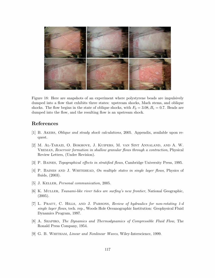
Figure 18: Here are snapshots of an experiment where polystyrene beads are impulsivelydumped into a flow that exhibits three states: upstream shocks, Mach stems, and obliqueshocks. The flow begins in the state of oblique shocks, with F0 = 3.08, Bc = 0.7. Beads aredumped into the flow, and the resulting flow is an upstream shock.

References

[1] B. Akers, Oblique and steady shock calculations, 2005. Appendix, available upon re-quest.

[2] M. Al-Tarazi, O. Bokhove, J. Kuipers, M. van Sint Annaland, and A. W.

Vreman, Reservoir formation in shallow granular flows through a contraction, PhysicalReview Letters, (Under Revision).

[3] P. Baines, Topographical effects in stratified flows, Cambridge University Press, 1995.

[4] P. Baines and J. Whitehead, On multiple states in single layer flows, Physics offluids, (2003).

[5] J. Keller, Personal communication, 2005.

[6] K. Muller, Tsunami-like river tides are surfing’s new frontier, National Geographic,(2005).

[7] L. Pratt, C. Hills, and J. Parsons, Review of hydraulics for non-rotating 1-d

single layer flows, tech. rep., Woods Hole Oceanographic Institution: Geophysical FluidDynamics Program, 1997.

[8] A. Shapiro, The Dynamics and Thermodynamics of Compressible Fluid Flow, TheRonald Press Company, 1954.

[9] G. B. Whitham, Linear and Nonlinear Waves, Wiley-Interscience, 1999.

117