Service Life Estimations in the Design of a PCM Based Night Cooling System

KTH Research School

Centre for Built Environment

Department of Technology and

Built Environment

University of Gävle

Service Life Estimations in the Design of a PCM Based Night Cooling System

Göran Hed

Doctoral Thesis

Gävle, Sweden, October 2005

ii

Department of Technology and Built Environment

University of Gävle

SE-801 76 Gävle SWEDEN

BMG-MT TR02-2005

ISBN 91-7178-141-2

Printed in Sweden by AB Öberghs Ljuskopia, Gävle

iii

Det enda bestående är förändringen.

Herakleitos

iv

v

ABSTRACT The use of Phase Change Material, PCM, to change the thermal inertia of lightweight buildings is investigated in the CRAFT project C-TIDE. It is a joint project with Italian and Swedish partners, representing both industry and research. PCMs are materials where the phase change enthalpy can be used for thermal storage. The Swedish application is a night ventilation system where cold night air is used to solidify the PCM. The PCM is melted in the day with warm indoor air and thereby the indoor air is cooled. The system is intended for light weight buildings with an overproduction of heat during daytime. In the thesis, the results of experiments and numerical simulations of the application are presented. The theoretical background in order design the heat exchanger and applying the installation in thermal simulation software is presented.

An extensive program is set up, in order to develop test methods and carry tests to evaluate the performance over time of the PCM. Testing procedures are set up according to ISO standards concerning service life testing. The tests are focused on the change over time of the Thermal Storage Capacity (TSC) in different temperature spans. Measurements are carried out on large samples with a water bath calorimeter. The service life estimation of a material is based on the performance of one or more critical properties over time. When the performances of these properties are below the performance requirements, the material has reached its service life. The critical properties of the PCM are evaluated by simulation of the application. The performance requirements of the material are set up according to general requirements of PCM and requirements according to building legislation. The critical properties of a PCM are the transition temperature, the melting temperature range and the TSC in the operative temperature interval. The critical property of the application is its energy efficiency.

The results of the study show that the night cooling system will lower the indoor air temperature during daytime. It also shows that the tested PCM does not have a clear phase change, but an increased specific heat in the operative temperature interval. Increasing the amount of material, used in the application, can compensate this. Finally, the tested PCM is thermally stable and the service life of the product is within the range of the design lives of the building services.

It is essential to for all designers to know the performance over time of the properties of PCMs. Therefore it is desirable that standardized testing methods of PCM are established and standardized classification systems of PCMs are developed.

vi

vii

PREFACE This thesis is the result of research in the area of service life planning. It started in 1997 in the R&D project concrete modular building system. The project was carried out in co-operation with KTH-BMG, LTH and a group of SMEs. The R&D project was connected to a prototype building situated in Gävle, Sweden, which was erected during the autumn 1999. My part of the work has, beside from the project leading, been the service life planning of the building. The result of the service life planning was presented in my licentiate thesis. Tutor was Professor Christer Sjöström. The project was financed with funds from European Union Objective 6, County Administrative Board of Gävleborg, The Swedish Council for Building Research (BFR), The Development Fund of the Swedish Construction Industry (SBUF) and Concrete Volume Sweden (CVS).

In 2000 I left the university for work in the building industry. In 2002 I was employed as teacher and researcher at University of Gävle. That engaged me in the research and development project C-TIDE.

In the CRAFT project C-TIDE (Changeable Thermal Inertia Dry Enclosures) the possibility of changing the thermal inertia of lightweight buildings with PCM, Phase Change Material, is explored. PCM was at that time a new experience for me. My familiar areas are service life planning and general building technology. In the interesting project I have combined these two areas with new knowledge about PCM and its integration in buildings.

I wish thank my supervisor Christer Sjöström who started the C-TIDE project at HiG and made it possible for me to come back to the university. Ove Söderström who is the second supervisor and my mathematical support and discussion partner. Marco Imperadori who came up with the idea of the C-TIDE project. Rickard Bellander who is my partner in the project and is the practical man. Our Italian guest researchers Davide and Allesandro helped us with the laboratory work. The PCM enthusiast Rolf Ulvengren and his company Climator AB who happily provided all the PCM that we needed for the work. HiG supported me in the writing of the thesis. I also wish to thank my family, my wife Annika and my children Anders and Anna who always support me.

Gävle in September 2005

Göran Hed

viii

ix

TABLE OF CONTENTS

1 INTRODUCTION ............................................................................................................. 1 1.1 Introduction 1 1.2 Service life planning 1

1.2.1 ISO standard .......................................................................................................... 1 1.2.2 Identification of critical properties ........................................................................ 4

1.3 Research project 6 1.4 Climatic context 8 1.5 Phase change materials - PCM 9

1.5.1 Thermal energy storage ......................................................................................... 9 1.5.2 Performance requirements of phase change materials........................................ 11 1.5.3 The use of PCM in building applications – thermal inertia................................. 13

1.6 Objectives 15 1.7 Limitations 15 1.8 Introduction of thesis 16

2 SUMMARY OF APPENDED PAPERS AND LICENTIATE THESIS..................... 17 2.1 Summary of licentiate thesis 17 2.2 Relationship between this thesis and licentiate thesis 17 2.3 Paper I 17 2.4 Paper II 18 2.5 Paper III 18 2.6 Paper IV 18 2.7 Paper V 19 2.8 Paper VI 19 2.9 Paper VII 19

3 METHOD......................................................................................................................... 21 3.1 RC network - Finite difference method 21 3.2 Water calorimeter measurements of PCM 23

3.2.1 Measurements and equipment.............................................................................. 23 3.2.2 Simulation of water calorimeter........................................................................... 24

3.3 PCM air heat exchanger 26 3.3.1 Mathematical formulation of air heat exchanger. ............................................... 26 3.3.2 Heat transfer coefficient....................................................................................... 26 3.3.3 Heat exchanger modelled with a single node finite difference model.................. 28

3.4 Room simulation 29 3.5 Test of application 30

3.5.1 Test room.............................................................................................................. 30 3.5.2 Simulation of test room ........................................................................................ 34

4 RESULTS OF MEASUREMENTS AND SIMULATIONS ........................................ 37 4.1 Results of water calorimeter measurements 37

4.1.1 Estimation of cP(T) curve ..................................................................................... 37 4.2 Air heat exchanger 42

4.2.1 Comparison between natural convection and heat exchanger ............................ 42 4.3 Room simulation 46 4.4 Results of temperature measurements and simulations in test room 50

4.4.1 Room air temperatures......................................................................................... 50 4.4.2 PCM temperatures ............................................................................................... 52

x

4.4.3 Simulations of test room with different PCM....................................................... 54 4.4.4 Cooling power ...................................................................................................... 59

5 DISCUSSION................................................................................................................... 63 5.1 General 63 5.2 Discussion of experimental results 64

5.2.1 Calorimeter .......................................................................................................... 64 5.2.2 Heat exchanger .................................................................................................... 66 5.2.3 Test room.............................................................................................................. 67 5.2.4 Comparison of accelerated and in use conditions ............................................... 68 5.2.5 Energy efficiency of the system ............................................................................ 69

5.3 Service life of PCM 70 5.3.1 Performance requirements................................................................................... 70 5.3.2 Critical properties of application......................................................................... 71 5.3.3 Degradation environment .................................................................................... 71 5.3.4 Service life discussion .......................................................................................... 71

6 CONCLUSIONS.............................................................................................................. 73

7 FUTURE WORK............................................................................................................. 75

8 REFERENCES ................................................................................................................ 77

xi

LIST OF APPENDED PAPERS

PAPER I HED, G., 1998. Service Life Planning in Building Design. CIB World Building Congress 1998, Gävle Sweden 7-12 June, Symposium A, Vol. 1 p. 201-209, ISBN 91-630-6711-0.

PAPER II HED, G., 1999. Service life planning of building components. 8th International Conference on Durability of Building Materials and Components, Vancouver, Canada, Vol. 2, ISBN 0-660-17741-2

PAPER III HED, G., 1999. Service life planning carried out in a building project. Published in: The International Journal of Low Energy and Sustainable Buildings, ISSN 1403-2147. http://www.byv.kth.se/avd/byte/leas/ (2005-08-22).

PAPER IV HED G., 2004. Use of phase change material for change of thermal inertia of buildings. 6th Expert Meeting and Workshop of Annex 17, 2004-06-07—09, Arvika, Sweden. http://www.fskab.com/Annex17/index.htm (2005-08-22).

PAPER V HED G, BELLANDER R., 2005. Service life testing of PCM based components in buildings. 10DBMC International Conférence On Durability of Building Materials and Components, LYON [France] 17-20 April 2005

PAPER VI HED G, BELLANDER R., 2005. Mathematical modelling of PCM air heat exchanger. Energy and buildings. (Article in press)

PAPER VII BELLANDER, R., HED, G. 2005. Calorimetric measurements of large samples of PCM. Energy and buildings. (Submitted)

PAPER I, PAPER II and PAPER III are also presented in the Licentiate Thesis:

HED G., 2000. Service life planning in building design. Thesis (Lic.). Centre of Built Environment, University of Gävle. Research School on Built Environment. RD-report No 4.

xii

xiii

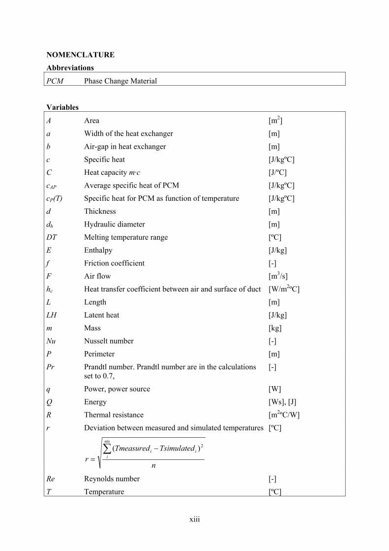
NOMENCLATURE

Abbreviations

PCM Phase Change Material

Variables

A Area [m2]

a Width of the heat exchanger [m]

b Air-gap in heat exchanger [m]

c Specific heat [J/kgºC]

C Heat capacity m·c [J/ºC]

cAP Average specific heat of PCM [J/kgºC]

cP(T) Specific heat for PCM as function of temperature [J/kgºC]

d Thickness [m]

dh Hydraulic diameter [m]

DT Melting temperature range [ºC]

E Enthalpy [J/kg]

f Friction coefficient [-]

F Air flow [m3/s]

hc Heat transfer coefficient between air and surface of duct [W/m2ºC]

L Length [m]

LH Latent heat [J/kg]

m Mass [kg]

Nu Nusselt number [-]

P Perimeter [m]

Pr Prandtl number. Prandtl number are in the calculations set to 0.7,

[-]

q Power, power source [W]

Q Energy [Ws], [J]

R Thermal resistance [m2ºC/W]

r Deviation between measured and simulated temperatures

n

TsimulatedTmeasuredr

nts

iii∑ −

=

2)(

[ºC]

Re Reynolds number [-]

T Temperature [ºC]

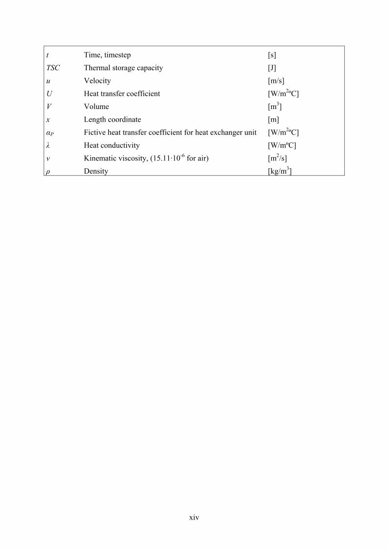
xiv

t Time, timestep [s]

TSC Thermal storage capacity [J]

u Velocity [m/s]

U Heat transfer coefficient [W/m2ºC]

V Volume [m3]

x Length coordinate [m]

αP Fictive heat transfer coefficient for heat exchanger unit [W/m2ºC]

λ Heat conductivity [W/mºC]

ν Kinematic viscosity, (15.11·10-6 for air) [m2/s]

ρ Density [kg/m3]

xv

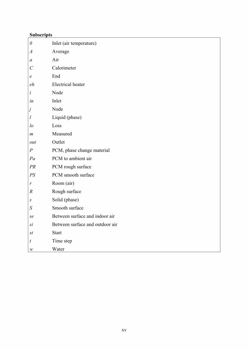
Subscripts

0 Inlet (air temperature)

A Average

a Air

C Calorimeter

e End

eh Electrical heater

i Node

in Inlet

j Node

l Liquid (phase)

lo Loss

m Measured

out Outlet

P PCM, phase change material

Pa PCM to ambient air

PR PCM rough surface

PS PCM smooth surface

r Room (air)

R Rough surface

s Solid (phase)

S Smooth surface

se Between surface and indoor air

si Between surface and outdoor air

st Start

t Time step

w Water

xvi

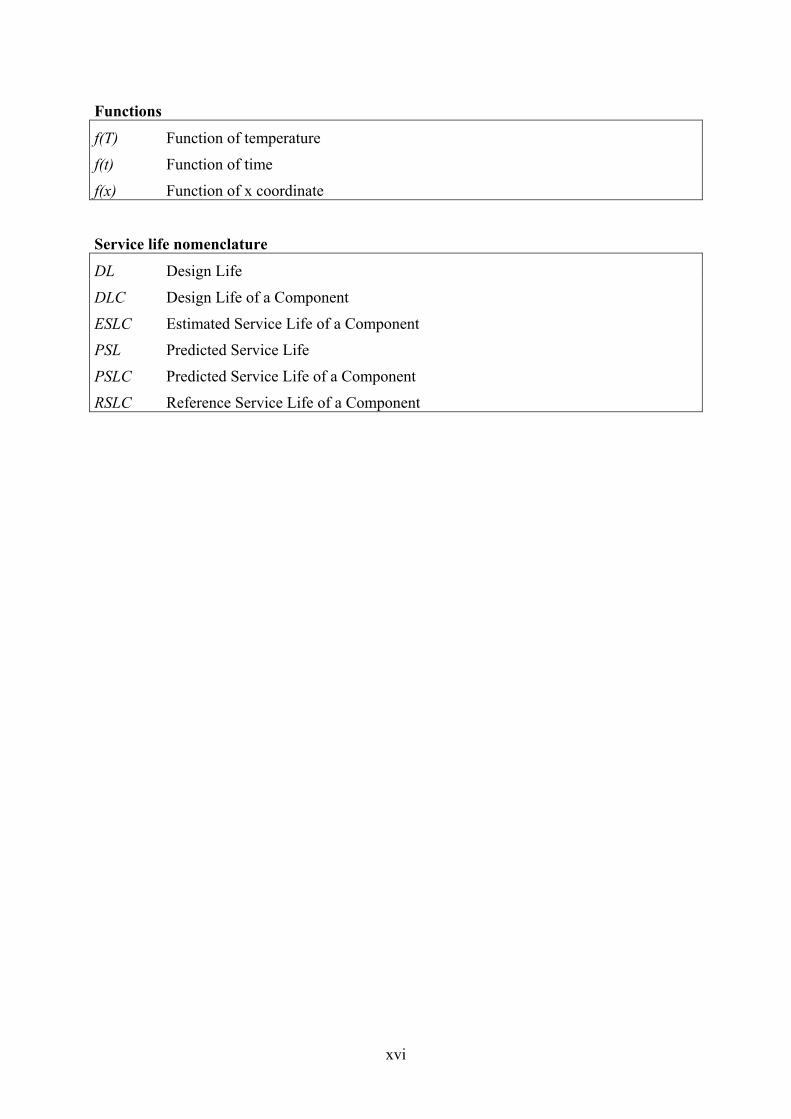
Functions

f(T) Function of temperature

f(t) Function of time

f(x) Function of x coordinate

Service life nomenclature

DL Design Life

DLC Design Life of a Component

ESLC Estimated Service Life of a Component

PSL Predicted Service Life

PSLC Predicted Service Life of a Component

RSLC Reference Service Life of a Component

1

1 INTRODUCTION

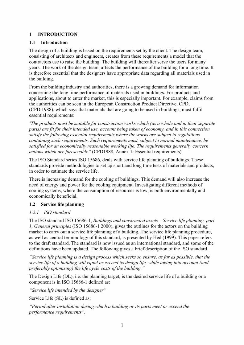
1.1 Introduction The design of a building is based on the requirements set by the client. The design team, consisting of architects and engineers, creates from these requirements a model that the contractors use to raise the building. The building will thereafter serve the users for many years. The work of the design team, affects the performance of the building for a long time. It is therefore essential that the designers have appropriate data regarding all materials used in the building.

From the building industry and authorities, there is a growing demand for information concerning the long time performance of materials used in buildings. For products and applications, about to enter the market, this is especially important. For example, claims from the authorities can be seen in the European Construction Product Directive, CPD, (CPD 1988), which says that materials that are going to be used in buildings, must fulfil essential requirements:

“The products must be suitable for construction works which (as a whole and in their separate parts) are fit for their intended use, account being taken of economy, and in this connection satisfy the following essential requirements where the works are subject to regulations containing such requirements. Such requirements must, subject to normal maintenance, be satisfied for an economically reasonable working life. The requirements generally concern actions which are foreseeable” (CPD1988, Annex 1: Essential requirements).

The ISO Standard series ISO 15686, deals with service life planning of buildings. These standards provide methodologies to set up short and long time tests of materials and products, in order to estimate the service life.

There is increasing demand for the cooling of buildings. This demand will also increase the need of energy and power for the cooling equipment. Investigating different methods of cooling systems, where the consumption of resources is low, is both environmentally and economically beneficial.

1.2 Service life planning

1.2.1 ISO standard

The ISO standard ISO 15686-1, Buildings and constructed assets – Service life planning, part 1, General principles (ISO 15686-1 2000), gives the outlines for the actors on the building market to carry out a service life planning of a building. The service life planning procedure, as well as central terminology of this standard, is presented by Hed (1999). This paper refers to the draft standard. The standard is now issued as an international standard, and some of the definitions have been updated. The following gives a brief description of the ISO standard.

“Service life planning is a design process which seeks so ensure, as far as possible, that the service life of a building will equal or exceed its design life, while taking into account (and preferably optimising) the life cycle costs of the building.”

The Design Life (DL), i.e. the planning target, is the desired service life of a building or a component is in ISO 15686-1 defined as:

“Service life intended by the designer”

Service Life (SL) is defined as:

“Period after installation during which a building or its parts meet or exceed the performance requirements”.

2

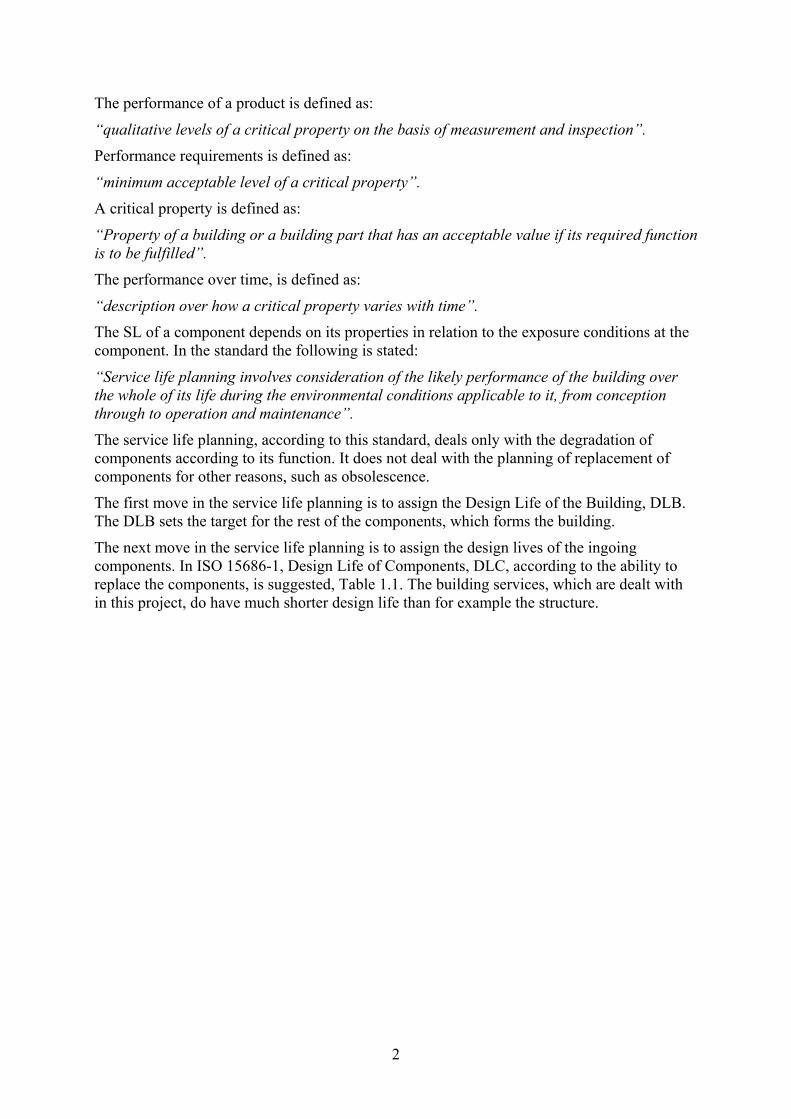
The performance of a product is defined as:

“qualitative levels of a critical property on the basis of measurement and inspection”.

Performance requirements is defined as:

“minimum acceptable level of a critical property”.

A critical property is defined as:

“Property of a building or a building part that has an acceptable value if its required function is to be fulfilled”.

The performance over time, is defined as:

“description over how a critical property varies with time”. The SL of a component depends on its properties in relation to the exposure conditions at the component. In the standard the following is stated:

“Service life planning involves consideration of the likely performance of the building over the whole of its life during the environmental conditions applicable to it, from conception through to operation and maintenance”.

The service life planning, according to this standard, deals only with the degradation of components according to its function. It does not deal with the planning of replacement of components for other reasons, such as obsolescence.

The first move in the service life planning is to assign the Design Life of the Building, DLB. The DLB sets the target for the rest of the components, which forms the building.

The next move in the service life planning is to assign the design lives of the ingoing components. In ISO 15686-1, Design Life of Components, DLC, according to the ability to replace the components, is suggested, Table 1.1. The building services, which are dealt with in this project, do have much shorter design life than for example the structure.

3

Table 1.1. Suggested minimum design lives for components (DLC) (Table 1,ISO 15686-1 2000)

A necessary process in the service life planning is the forecasting of the service life of the component. The forecasted service life should equal or exceed the DL of the component. The forecasting can be based on different methods. Dependent on which method the forecasting is based on, it can be referred to differently.

If the forecasting is based on tests that are carried out according to the procedures described in ISO 15686-2 (2001). Buildings and constructed assets – Service life planning, part 2, Service life prediction principles, it should be referred to as Predicted Service Life, PSL, or Predicted Service Life of a Component, PSLC, the following condition must be fulfilled

PSLC ≥ DLC

If the component is exposed to a different exposure situation, it can be adjusted using the factor method. The factor method is described in Chapter 9 of the standard (ISO 15686-1, 2000) (Marteinsson 2003). If the forecasting is based on the factor method, it should be referred to as ESLC, Estimated Service Life of a Component. Hence,

ESLC ≥ DLC

Design life of building

Inaccessible or structural

components

Components where

replacement is expensive or

difficult (including below ground drainage)

Major replaceable components

Building services

Unlimited Unlimited 100 40 25

150 150 100 40 25

100 100 100 40 25

60 60 60 40 25

25 25 25 25 25

15 15 15 15 15

10 10 10 10 10

NOTE 1 Easy to replace components may have design lives of 3 to 6 years

NOTE 2 Unlimited design life should very rarely be used, as it significantly reduces design options

4

With the factor method it should be possible to consider local variations and take into account a variety of factors that will affect the service life of a product. The factor method is concluded in the following formula:

ESLC = RSLC · A · B · C · D · E · F · G

where the modifying factors reflects:

• A: quality of component

• B: design level

• C: work execution level

• D: indoor environment

• E: outdoor environment

• F: in-use conditions

• G: maintenance level

In this project specific tests are carried out to according to the procedure referred to in ISO 15686-2 (2001). The general procedure is outlined in Figure 1.1.

1.2.2 Identification of critical properties

The prediction of the service life of a component, should be based on the performance over time of one or more critical properties. One of the aims of the theoretical and experimental work in the project, is to evaluate which properties or change of properties are critical to the overall performance of the application. The properties can vary both with time and with temperature. A numerical simulation model where termal properties can be assigned to the material, is used for this purpose.

It is assumed that the operative temperature interval is of great importance in the testing method. Earlier tests by Johansson (2001) and Heteny (1981) were made using Differential Thermal Analysis, DTA, on small samples. The specimen size and the geometry might also have an influence of the behaviour of the material. In the DTA, the sample weight is about 400 mg. In the test presented in this thesis the sample weight is approximately 1.5 kg.

The tests by Johansson and Heteny were carried out in a temperature range of 15 to 35ºC. This temperature range is greater than the operative temperature range of the application, which is 24±3-4ºC. If the melting temperature range of the PCM is large, it may not be possible to charge and discharge the PCM within the operative temperature span. Matching the transition temperature range, for a given application, is an important aspect of PCM thermal storage design (He 2004).

5

Figure 1.1. Principal for testing procedure (ISO 15686-2 2001)

6

1.3 Research project In the CRAFT project C-TIDE (Changeable Thermal Inertia Dry Enclosures), the possibility of the use of PCM in order to increase the thermal inertia of lightweight buildings is explored. The project is performed in collaboration with Italian and Swedish partners, representing both industry and research. Two different approaches of the integration of the PCM are taken in Italy and Sweden. The Swedish group investigates the possibility to place the PCM inside a building and actively, with fans, absorb and release energy. In the Italian project the PCM is integrated in the façade of a building, in order to absorb the heat from solar radiation and high air temperatures. Different arrangements in the outer shell are investigated by measurements on experiment buildings. Regardless of type of integration of the material, the performance over time of the PCM is of crucial importance for the function of any such system.

The work by the Swedish group deals with two issues: Performance over time of the PCM that is going to be used in a specific application. The thermal storage capacity over a specified temperature interval is measured to see if there is a change of the performance, when the PCM is exposed to temperature cycling. The tests are carried out using a water bath calorimeter.

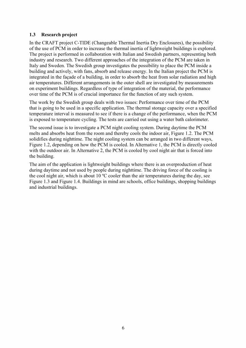
The second issue is to investigate a PCM night cooling system. During daytime the PCM melts and absorbs heat from the room and thereby cools the indoor air, Figure 1.2. The PCM solidifies during nighttime. The night cooling system can be arranged in two different ways, Figure 1.2, depending on how the PCM is cooled. In Alternative 1, the PCM is directly cooled with the outdoor air. In Alternative 2, the PCM is cooled by cool night air that is forced into the building.

The aim of the application is lightweight buildings where there is an overproduction of heat during daytime and not used by people during nighttime. The driving force of the cooling is the cool night air, which is about 10 ºC cooler than the air temperatures during the day, see Figure 1.3 and Figure 1.4. Buildings in mind are schools, office buildings, shopping buildings and industrial buildings.

7

Figure 1.2. Principal function of PCM night cooling system. During the day (DAY CASE) the PCM is melting. During night (NIGHT CASE) the PCM is solidified. The PCM cooling system works independent of the normal ventilation system of the building.

8

1012141618202224262830

196 197 198 199 200 201 202 203

Day

Tem

pera

ture

[ºC]

0102030405060708090

100

-5 0 5 10 15 20

Temperature [ºC]

%

1.4 Climatic context The driving force of the cooling application is the cool night air temperature. Normally, there is a temperature difference of at least 10 °C from day to night on a warm day in Sweden. This is shown by measurements of temperatures in 2002 in Gävle, Sweden. The simulations performed in the preliminary studies of the system, are based on these data. In Figure 1.3 the night temperatures at 01.00 from May to October 2002, are shown.

Figure 1.3. Cumulative distribution of night air temperatures at 01.00 in Gävle from May to October 2002

In Figure 1.4 a typical week with high air temperatures are shown. For the application the most interesting information is the night temperatures during the summer months. The highest night temperature during the cooling is what decides the lowest melting temperature of the PCM, that is going to be used. It must be possible to solidify the PCM with the cool night air.

Other important information found in the climatic data, is the length of time, during which the cool night temperature is available. This sets the requirements of the heat transfer properties of the night cooling system.

Figure 1.4. Air temperatures in Gävle during the summer of 2002. Day 196 to 203 ( 15th to 22nd of July).

9

1.5 Phase change materials - PCM

1.5.1 Thermal energy storage

Energy storage, affected by a temperature change, can take place in two ways. With sensible heat, the storage capacity is linearly dependent on the temperature change and the specific heat of the material. With latent heat the storage capacity is dependent on the phase change enthalpy of the material. A Phase Change Material, PCM, is a material where there is a change of phase from liquid to solid or gas to liquid and the opposite, over a limited temperature interval. During the phase change large amounts of energy can be stored or released (Pillai 1976, Hasnain 1998, Farid 2003).

The phase change can be described with a specific heat curve, cP(T), where the phase change is described as an increase of the specific heat in a temperature interval. The Thermal Storage Capacity, TSC, in a temperature interval from T1 to T2 for a PCM is:

∫=2

1

)(),( 21

T

TPP dTTcmTTTSC [ 1.1]

If the start and end temperatures are the temperatures of the phase change, the TSC divided by mass is commonly referred to as the Latent Heat (LH) of the PCM.

If the phase change takes place over a temperature interval, it is referred to as the melting temperature range, DT. The shape of the cP(T) curve can vary. In this thesis, two shapes are used in the calculations and simulations, one with a trapezoidal shape and one with a cosine shape. It is also assumed that the cP(T) curve is the same for melting and solidification, Figure 1.5. The super cooling effect in the material is not considered in the cP(T) curve.

The curves used in the calculations are described with a code, described with the following examples:

PC24 DT8 and PC24c DT8,

where PC24 is the phase change temperature.

The subscript c is the cosine shape.

DT8 is the melting temperature range of 8ºC.

Figure 1.5. Examples of cP(T) curves used in the calculations and evaluations of the PCM. Left curve has a trapezoidal shape, right curve has a cosine shape. DT and TSC over the temperature interval DT is the same.

12 15 18 21 24 27 30 33 360

4000

8000

1.2 .104

1.6 .104

2 .104

cP T( )

T

12 15 18 21 24 27 30 33 360

4000

8000

1.2 .104

1.6 .104

2 .104

cP T( )

T

10

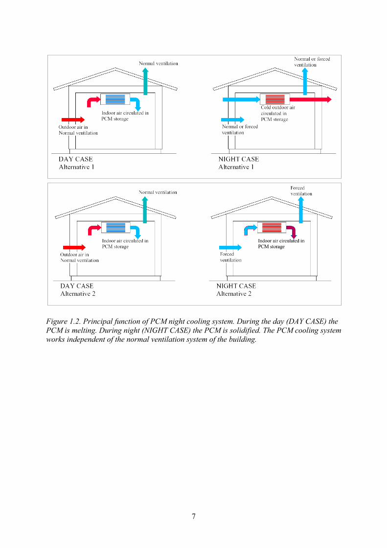
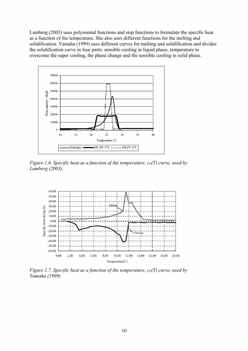
Lamberg (2003) uses polynomial functions and step functions to formulate the specific heat as a function of the temperature. She also uses different functions for the melting and solidification. Yamaha (1999) uses different curves for melting and solidification and divides the solidification curve in four parts: sensible cooling in liquid phase, temperature to overcome the super cooling, the phase change and the sensible cooling in solid phase.

Figure 1.6. Specific heat as a function of the temperature, cP(T) curve, used by Lamberg (2003).

Figure 1.7. Specific heat as a function of the temperature, cP(T) curve, used by Yamaha (1999)

11

1.5.2 Performance requirements of phase change materials

For the use of PCMs in night cooling applications, where no heat pumps are used, the following requirements, relating to the phase change temperature, must be fulfilled. The melting temperature must be close to the system operative temperature range. This means that the phase change temperature must be close to room temperature. It must be lower than the highest acceptable room temperature. The melting temperature range of the PCM must be within an acceptable range. Otherwise the function of the system is jeopardized. This issue is discussed in Paper VI. It must be possible to solidify the material with the night outdoor temperature. The phase change temperature is an important property for the PCM. For change of thermal inertia using cool night air, a melting temperature close to room temperature is suitable. The melting temperature cannot be too low, because it must be possible to solidify the PCM with the outdoor night air.

Two main groups of PCM are available at the market: organic and inorganic. Organic materials are fat, oil and waxes. The inorganic materials are for example salts, salt solutions and salt hydrates. Lists of materials are available in, for instance, Zalba (2003).

Different authors have listed main criteria for PCM, Table 1.2:

Table 1.2. Requirements of PCM, He (2004), Abhat (1983) and Pillai (1976)

No Condition

1 The phase transition process must be completely reversible and only temperature dependent.

2 The phase transition temperature must match the practical temperature range of the application.

3 The material must have a large latent heat and high thermal conductivity. The material is chemically stable so that no chemical composition occurs.

4 The material must be non-toxic, non-corrosive and non-explosive.

5 The material must be available in large quantities at low cost.

12

The use of PCM in building applications has special material requirements. According to the CPD (CPD 1988) six essential requirements must be fulfilled for materials. These are shown in Table 1.3.

Table 1.3. Six essential requirements according to CPD.

No Requirement

1 Mechanical resistance and stability.

2 Safety in case of fire.

3 Hygiene, health and environment.

4 Safety in use.

5 Protection against noise.

6 Energy economy and heat retention.

The material that is tested in the research programme is based on hydrated salt, Na2SO4·10H2O. This is named Glauber’s salt. The advantages with Glauber’s salt and other salt hydrates are high heats of fusion, not being flammable, and low price (Martin 2003).

The pure Glauber’s salt faces two main problems due to incongruent melting. These are super cooling and phase separation. Super cooling or sub cooling occurs in the solidification of a material and can be described as the temperature below the solidification temperature needed to start the solidification. Pure Glauber’s salt has a severe problem with super cooling. It can be as high as 15-18˚C (Ruy 1992). The melting temperature is about 32˚C, which means that the temperature must be lowered to 14-17˚C in order to start the solidifying of the material. To overcome these problems a nucleating agent is added to the salt. Byung (1989) and Ruy (1992) suggest that Borax (Na2B2O7·10H2O) can be used for this purpose; this can reduce the super cooling to 3-4˚C.

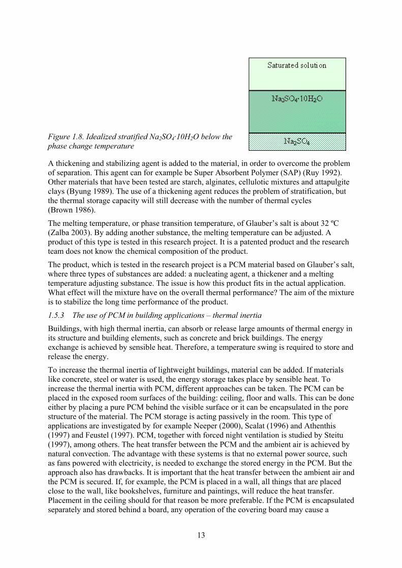
The other main problem with Glauber’s salt is the separation of the salt. The salt hydrate separates to saturated solution, salt hydrate and salt. The three different phases have different densities and thereby a stratification of the material occurs. The density of the saturated solution is 1320 kg/m3, the salt hydrate 1460 kg/m3and the salt 2660 kg/m3 (Stockerl 1991, Carlsson 1978). An idealized picture of the stratification is shown in Figure 1.8. This problem arises with thermal cycling.

13

Figure 1.8. Idealized stratified Na2SO4·10H2O below the phase change temperature

A thickening and stabilizing agent is added to the material, in order to overcome the problem of separation. This agent can for example be Super Absorbent Polymer (SAP) (Ruy 1992). Other materials that have been tested are starch, alginates, cellulotic mixtures and attapulgite clays (Byung 1989). The use of a thickening agent reduces the problem of stratification, but the thermal storage capacity will still decrease with the number of thermal cycles (Brown 1986).

The melting temperature, or phase transition temperature, of Glauber’s salt is about 32 ºC (Zalba 2003). By adding another substance, the melting temperature can be adjusted. A product of this type is tested in this research project. It is a patented product and the research team does not know the chemical composition of the product.

The product, which is tested in the research project is a PCM material based on Glauber’s salt, where three types of substances are added: a nucleating agent, a thickener and a melting temperature adjusting substance. The issue is how this product fits in the actual application. What effect will the mixture have on the overall thermal performance? The aim of the mixture is to stabilize the long time performance of the product.

1.5.3 The use of PCM in building applications – thermal inertia

Buildings, with high thermal inertia, can absorb or release large amounts of thermal energy in its structure and building elements, such as concrete and brick buildings. The energy exchange is achieved by sensible heat. Therefore, a temperature swing is required to store and release the energy.

To increase the thermal inertia of lightweight buildings, material can be added. If materials like concrete, steel or water is used, the energy storage takes place by sensible heat. To increase the thermal inertia with PCM, different approaches can be taken. The PCM can be placed in the exposed room surfaces of the building: ceiling, floor and walls. This can be done either by placing a pure PCM behind the visible surface or it can be encapsulated in the pore structure of the material. The PCM storage is acting passively in the room. This type of applications are investigated by for example Neeper (2000), Scalat (1996) and Athenthis (1997) and Feustel (1997). PCM, together with forced night ventilation is studied by Steitu (1997), among others. The heat transfer between the PCM and the ambient air is achieved by natural convection. The advantage with these systems is that no external power source, such as fans powered with electricity, is needed to exchange the stored energy in the PCM. But the approach also has drawbacks. It is important that the heat transfer between the ambient air and the PCM is secured. If, for example, the PCM is placed in a wall, all things that are placed close to the wall, like bookshelves, furniture and paintings, will reduce the heat transfer. Placement in the ceiling should for that reason be more preferable. If the PCM is encapsulated separately and stored behind a board, any operation of the covering board may cause a

14

punctuation of the encapsulation. The boards will also reduce the heat transfer. For these reasons, placement in a false ceiling covered with metal is to prefer.

The other approach is that the PCM is placed in a storage unit and the energy is exchanged actively by the use of fans. By forcing the warm/cold air into the storage, a better control of the performance can be achieved. Banard (2002) reports of the Cool Deck application, an installation where cold night air is forced into a concrete structure. The installation has also in a later phase been completed with PCM. In the TermoDeck system, cold night air is circulated in concrete hollow deck. This system is reported for instance by Winwood (1997) and Barton (2002). A drawback of the use of fans to exchange the energy, is that power of the fans can exceed the cooling power output from the exchanger. The variation over time of cooling power output from the exchanger is highly dependent on the melting temperature range of the PCM.

In Paper IV, simulations of a night cooling application are carried out for buildings with different thermal inertia, with and without added PCM. The simulations showed that the effect on the indoor temperature is similar in a light weight building where PCM is added, and a heavyweight building without PCM. Adding PCM in a heavyweight building gives a limited effect. Lamberg (2000) shows that PCM in concrete buildings has a low effect on the indoor climate.

15

1.6 Objectives In the design of a building, it is essential to know the performance over time of chosen components. Requirements, both in the long and short run, determined by authorities and the users of the building, must be met. Weathering agents and other degrading agents that will affect the performance, must be considered. Also, economic and environmental aspects have to be taken into account. Special attention needs therefore to be taken for new materials and applications that will enter the market. PCMs can be used in buildings to store energy, both in cooling and heating applications. For this group of materials, like for all other materials and building components, the designers must know the properties in order to make an appropriate design. Since the expected service life for buildings and its components are counted in tens of years, designers also must know if and how the material properties will change over time.

A particular PCM is studied in a night cooling application. The PCM is solidified (and cooled) with cool night air and used to cool the building on the following day. Experiments to evaluate the thermal properties and their changes over time are carried out. As guidance for the experimental set-up serves the international standard ISO 15686-2 Buildings and constructed assets – Service life planning, part 2, Service life prediction principles. This standard supports the service life demands of the CPD.

The objective of the study, presented in this thesis, is to evaluate the tested PCM’s ability to maintain its critical properties during its service life in the night cooling application. To determine which properties that are critical, a program is set up to investigate the actual application. The examined properties will form the basis, from which the service life of the PCM can be assessed.

1.7 Limitations

In this thesis, the building technology aspects of the use of PCM and its performance over time, is the main subject. This leads to certain limitations. It is not an intention to explain the chemical reactions that take place in the PCM, neither to describe the chemical composition of materials that are tested in the experimental work.

16

1.8 Introduction of thesis Chapter 1 is an introduction to the subjects that this thesis deals with, the service life planning and the use of phase change materials, PCM. An introduction is also given to the night cooling application that is studied in the C-TIDE project. In Chapter 3, an overview of the different methods that are used in the research project are presented. In the mathematical modelling the finite difference method is used. Measurements of the thermal properties are carried out with water calorimeter equipment. The investigated application consists of a PCM air heat exchanger that is installed in a test room. Chapter 4 consists of the results of the measurements of the material and the results of the measurements and simulation of the application. In Chapter 5 the results are discussed. Especially the aspect of service life of the PCM in its application is discussed. In Chapter 6 the discussion is concluded. Future studies of PCM are suggested in Chapter 7.

17

2 SUMMARY OF APPENDED PAPERS AND LICENTIATE THESIS

2.1 Summary of licentiate thesis In May 2000 the licentiate thesis: “Service Life Planning in Building Design” was presented. The main issue of this work was a general view of service life planning of buildings. The research is performed on a multi family building where the service life planning process is studied. The ISO standard ISO/DIS 15686.1 Buildings – Service Life Planning, Part 1, General Principles, is a base for the work. The service life planning is integrated in the design of the building and follows the building process from the design phase to the beginning of the construction of the building.

The service life planning begins with a planning phase where the goals are formulated. These are expressed as design lives, where the overarching goal is the design life of the building. Thereafter the design lives of installed components are established. The next phase in the work is to investigate whether the planning goals are satisfied or not, if the estimated service life of the components exceed the design life. The service life is estimated for about 30 different components in the building. The estimations are based on the performance over time of the components. The service life is reached when the performance for a critical property is below a critical level. All service life estimations are based on available data, i.e. no material research such as ageing tests and field inspections takes place within the project.

The conclusion of the study is that three different approaches could be used to assess the service life of a product. First is the “dose response approach” where gradual degradation of components takes place due to a specific dose of a degradation agent. The second approach is to draw conclusions of the service life from observed maintenance intervals in the built environment. Third is the “risk assessment approach”. It is adopted for such components that are not subjected to continuous degradation, but have an instant failure, due to special conditions.

2.2 Relationship between this thesis and licentiate thesis The research carried out in the C-TIDE project is a special case of service life planning, an investigation of new material that is about to enter the building market. At the time of publication of the licentiate thesis the standard “ISO/DIS 15686-1 Buildings – Service Life Planning, Part 1, General Principles” was a draft standard (ISO/DIS). Now this standard is released in the name of “ISO 15686-1:2000 Buildings and constructed assets - Service life planning - Part 1: General principles” (ISO 15686-1 2000).

The licentiate thesis deals with service life planning of a whole building, where the service life estimations could be used in the economical and maintenance planning of the building. In this thesis, the work is concentrated to a PCM night cooling application. As it will be installed in buildings and serve the building and the users for many years, it is important that the performance over time is known.

2.3 Paper I The principles for the service life planning, are given in the draft ISO standard Buildings Service Life Planning. The service life planning begins with an establishment of the Design Life of the Building, DLB. An economic DLB would be in the range of 30 to 60 years. This matter is discussed and the result is DLB=60 years. It is discussed how the Design Life of a Components, DLC, can be chosen. In service life estimations three different aspects have to be considered, the inherent properties, the degradation agents and the performance requirements of the actual component.

18

2.4 Paper II While Paper I discusses the set-up and the early stages of the service life planning, this paper deals with different methods for service life estimations. One task in the project is to test and evaluate the ISO standard, which is under development. This standard has during the carrying out of the project developed to a draft ISO standard, ISO/DIS 15686 Buildings – Service Life Planning, Part 1, General principles (ISO 15886-1). Parts of the standard are discussed. The principles for service life estimations established in the previous section are used and the results are presented in a table.

2.5 Paper III Paper III is a continuation of Paper I and Paper II. It discusses in more detail how the service life estimations are performed in the project and it analyses principle ways for further development. Three different approaches are used in the service life estimations. The first approach builds on the gradual degradation of components due to a specific dose of a degradation agent. It is named the “dose response approach”. In this method established dose response functions or damage functions are used. These functions are established from field tests where a degradation of a material is measured during a time period. The degradation environment is at the same time monitored. The functions are thereafter established by correlation analysis. Functions are established mainly for metals and some stone materials. The second way to estimate the service life is to draw conclusions of the service life from observed maintenance intervals on the built environment. Data also can be obtained from systematic field inspections. To strengthen this method further, the degradation environment can be monitored. The third approach is the “risk assessment approach”. It could be adopted for such components that are not subjected to continuous degradation but has an instant failure, due to special conditions. The service life should in this case be presented as a probability of occurrence in this particular condition. Examples of service life estimations are shown in the paper.

2.6 Paper IV In Paper IV simulations of a PCM based night cooling system is described where an ideal phase change material is installed in a building. This is the first study in order to see the effect of the indoor climate during a summer in Swedish climate. Three different buildings are simulated: a classroom, an office and a shopping centre. Each building is simulated as a lightweight, middleweight and a heavyweight building. The installation consists of PCM storage where the indoor air is circulated. The PCM is supposed to be stored in 10 to 20 mm layers in an air heat exchanger. In the mathematical model the PCM is supposed to maintain a steady temperature during its melting and solidifying.

The PCM is melted during daytime with the hot indoor air; the energy from the indoor air will be stored in the PCM. During night, cool outdoor air is circulated in the building with forced ventilation. This cool air mixes with the indoor air and is circulated in the PCM storage. Then the PCM will solidify and release the energy that is stored the day before. The PCM storage unit is operated with fans. The advantage of using this configuration is that the release and storage can be controlled. For example, if there is a cool day after a cool night there is no need to run the system and store energy from the indoor environment. The PCM is supposed to maintain a steady temperature during the phase change. Therefore it is modelled as a power source. The effect on the indoor air is linearly dependent on the airflow through the PCM unit and the temperature difference between the indoor air and the PCM. This assumption shows later in the research project to be too optimistic. It is found (see Paper VI and Paper VII) that the properties of the PCM are not as good as assumed. This leads to an overestimation of the cooling power of the PCM installation. A value too high is used in the simulations. Based on

19

these findings in the measurements, a modification of the simulation model is made (see Paper VI).

The model that is presented in the paper is supposed to give advice on how much PCM that is required in order to achieve desired goals of the installation. The information from the simulation is used to set up a test room. It is found that the amount of PCM is not sufficient to give the desired effect on the indoor climate. However, the findings from the research project will be fed into the model presented in this thesis for one of the simulated buildings.

2.7 Paper V In this paper the testing procedure of the PCM is described. The governing requirements of the PCM and its installation in a building are the six essential requirements of the CPD.The framework of the testing procedure is described in the international standard “ISO 15686-2, Buildings and Constructed assets – Service Life Planning, part 2, Service life prediction principles”. The outline of procedure is described in the scheme in Figure 1.1. In the paper it is discussed how the issues of definition, preparation, accelerated exposure and field exposure are implemented in the testing procedure. Measurements of the thermal storage capacity are carried out in a water bath calorimeter. The intention of the testing campaign is to resemble the actual use condition.

2.8 Paper VI

This paper deals with the mathematical formulation of the PCM heat exchanger. It is suggested that the heat exchanger unit can be represented with a fictive heat transfer coefficient, αP, where the heat transfer between the PCM and the air, is dependent on the geometry of the unit, the thickness of PCM layers and the air flow through the unit. The PCM is suggested to be modelled with a variable thermal specific heat, a cP(T) curve. The mathematical model is verified by measurements on a prototype heat exchanger.

2.9 Paper VII In this paper the accelerated testing procedure of the PCM is described. The PCM is thermally cycled in water baths and the TSC is measured with a water calorimeter. The testing is carried out on six different samples. Each sample is temperature cycled approximately 200 times, where measurements in the calorimeter are made in two thirds of the cycles. The results of the measuring campaign are presented in the paper. The phase change temperature according to the supplier of the PCM is 24 ºC and it is expected that the melting temperature range is close to this temperature. The measurements show that there is no phase change in the PCM in the operative temperature range. But compared to the liquid and solid phase there is an increase of the specific heat. The results of the calorimeter measurements are fed into the simulation models of the application.

20

21

3 METHOD

3.1 RC network - Finite difference method The water calorimeter, the heat exchanger and the test room, are modelled with a network of resistances and capacitances, a RC-network. A numerical solution is obtained with the finite difference method programmed in Mathcad (Mathsoft 2002). A heat balance for node i is established. Connecting nodes are denoted j and the time step is t. This results in a general form of the finite difference formulation, Figure 3.1.

−+⋅

∆+= ∑+

ji

titjjii

ititi R

TTAq

CtTT

,

,,,,1, [ 3.1]

where

ji

jiji

dR

,

,, λ

= [ 3.2]

and

iiii VcC ⋅⋅= ρ [ 3.3]

where T is the temperature, t is the time, q is an internal power source, d is the thickness of the material, λ is the thermal conductivity, c is the specific heat, ρ is the density and V is the volume.

Figure 3.1. RC-network model.

The phase change in the material is represented by an increase of the specific heat in the material over a temperature range, a cP(T) curve (Lamberg 2003). Bonacina (1973) states that this approach is sufficiently accurate for engineering use. The shape of this curve for the specific hydrated salt that is used in the project, is not known. Therefore, a function with parameters for the transition temperature, the melting temperature range and the specific heat is assumed.

22

Thus, the finite difference equation for the PCM node of the RC network is

−+⋅

∆+= ∑+

ji

titjjij

itiPtiti R

TTAq

TCtTT

,

,,,

,,1, )(

[ 3.4]

where

iitiPtiP VTcTC ⋅⋅= ρ)()( ,, [ 3.5]

This simplified model, gives the possibility to simulate the time dependent behaviour of the applications, where the PCM is used. It is used in the design and simulation of the water calorimeter, the heat exchanger and the room model. It is possible to model the time-dependent behaviour on both short and long term changes.

The primary use of the PCM in the research project is to change the thermal inertia of the building. Material properties and long time dependent properties are measured in the calorimeter measurements. The results of the measurements are thereafter fed into the models of the heat exchanger and the room model.

23

3.2 Water calorimeter measurements of PCM

3.2.1 Measurements and equipment

The measurement procedure and the equipment are described in Paper VII

The average specific heat is defined as

Pste

PAP mTT

Qc⋅−

=)(

[ 3.6]

where

∫ ⋅⋅=e

st

T

TPPp dT(T)cmQ [ 3.7]

QP is the energy that is stored in the PCM, mP is the mass of the PCM

Energy input from the electrical heater is

∫ ⋅=e

st

t

teheh dtqQ [ 3.8]

The losses from the measuring equipment can be written

)(( CCsterwlo AU)t(t)TTQ ⋅⋅−⋅−= ∑ [ 3.9]

where UC and AC are the heat transfer coefficient and the area of the equipment.

The energy balance is

loehP QQQ −= [ 3.10]

24

3.2.2 Simulation of water calorimeter

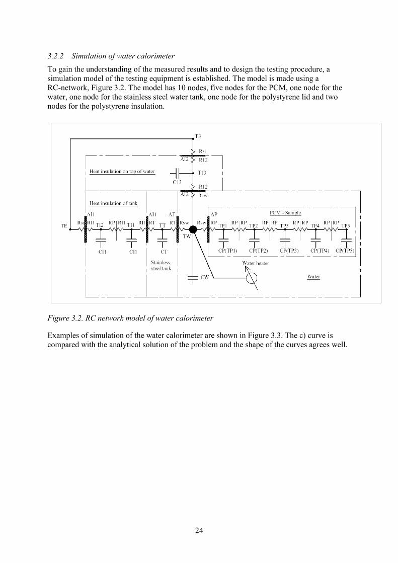
To gain the understanding of the measured results and to design the testing procedure, a simulation model of the testing equipment is established. The model is made using a RC-network, Figure 3.2. The model has 10 nodes, five nodes for the PCM, one node for the water, one node for the stainless steel water tank, one node for the polystyrene lid and two nodes for the polystyrene insulation.

Figure 3.2. RC network model of water calorimeter

Examples of simulation of the water calorimeter are shown in Figure 3.3. The c) curve is compared with the analytical solution of the problem and the shape of the curves agrees well.

25

a)

b)

c)

Figure 3.3. Examples of simulations to show the effect of different shapes of the cP(T). TP5 is the temperature in the middle of the sample. In a) there is a clear phase change in a narrow temperature interval 2ºC, PC24 DT2. In b) the melting temperature range is 14ºC, PC24 DT14. In c) no phase change takes place in the temperature interval.

0 0.2 0.4 0.6 0.8 110

20

30

40

50

TP5i

idt

60 60⋅⋅

16 20 24 28 320

1.2 .1042.4 .1043.6 .1044.8 .104

6 .104

cP T( )

T

T2 24= DT 14=

TSC18

28TcP T( )

⌠⌡

d:= TSC 100 103×=

0 0.2 0.4 0.6 0.8 110

20

30

40

50

TP5i

idt

60 60⋅⋅

16 20 24 28 320

1.2 .1042.4 .1043.6 .1044.8 .104

6 .104

cP T( )

T

T2 24= DT 2=

TSC18

28TcP T( )

⌠⌡

d:= TSC 100 103×=

0 0.2 0.4 0.6 0.8 110

20

30

40

50

TP5i

idt

60 60⋅⋅

16 20 24 28 320

1.2 .1042.4 .1043.6 .1044.8 .104

6 .104

cP T( )

T

T2 24= DT 2=

TSC18

28TcP T( )

⌠⌡

d:= TSC 100 103×=

26

3.3 PCM air heat exchanger

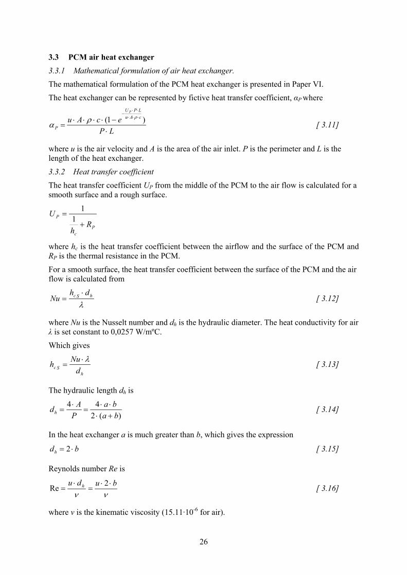
3.3.1 Mathematical formulation of air heat exchanger.

The mathematical formulation of the PCM heat exchanger is presented in Paper VI.

The heat exchanger can be represented by fictive heat transfer coefficient, αP where

LPecAu cAu

LPU

P

P

⋅−⋅⋅⋅⋅

=⋅⋅⋅⋅⋅

−

)1( ρρα [ 3.11]

where u is the air velocity and A is the area of the air inlet. P is the perimeter and L is the length of the heat exchanger.

3.3.2 Heat transfer coefficient

The heat transfer coefficient UP from the middle of the PCM to the air flow is calculated for a smooth surface and a rough surface.

Pc

P

Rh

U+

=1

1

where hc is the heat transfer coefficient between the airflow and the surface of the PCM and RP is the thermal resistance in the PCM.

For a smooth surface, the heat transfer coefficient between the surface of the PCM and the air flow is calculated from

λhSc dh

Nu⋅

= [ 3.12]

where Nu is the Nusselt number and dh is the hydraulic diameter. The heat conductivity for air λ is set constant to 0,0257 W/mºC.

Which gives

hSc d

Nuh λ⋅= [ 3.13]

The hydraulic length dh is

)(244

baba

PAdh +⋅

⋅⋅=

⋅= [ 3.14]

In the heat exchanger a is much greater than b, which gives the expression

bdh ⋅= 2 [ 3.15]

Reynolds number Re is

ννbudu h ⋅⋅

=⋅

=2Re [ 3.16]

where ν is the kinematic viscosity (15.11·10-6 for air).

27

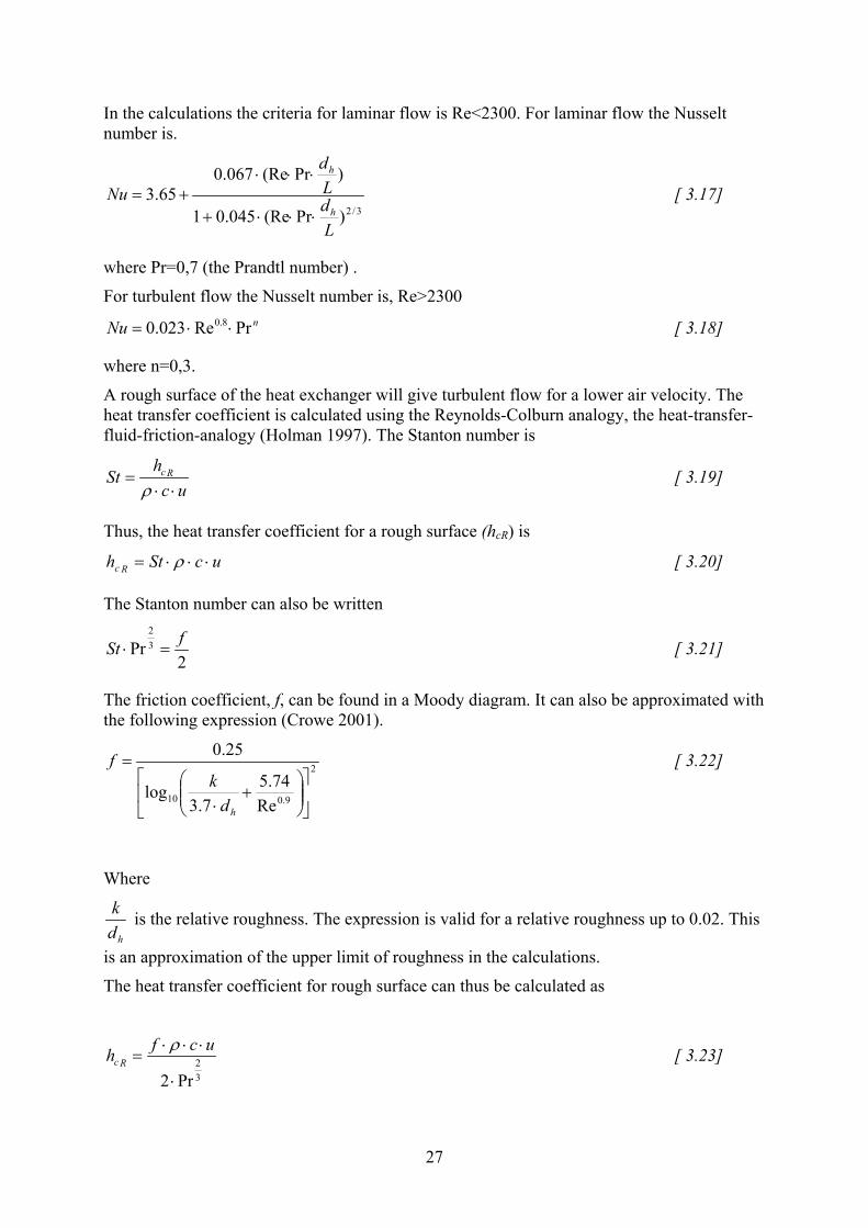
In the calculations the criteria for laminar flow is Re<2300. For laminar flow the Nusselt number is.

3/2)Pr(Re045.01

)Pr(Re067.065.3

LdLd

Nuh

h

⋅⋅⋅+

⋅⋅⋅+= [ 3.17]

where Pr=0,7 (the Prandtl number) .

For turbulent flow the Nusselt number is, Re>2300 nNu PrRe023.0 8.0 ⋅⋅= [ 3.18]

where n=0,3.

A rough surface of the heat exchanger will give turbulent flow for a lower air velocity. The heat transfer coefficient is calculated using the Reynolds-Colburn analogy, the heat-transfer-fluid-friction-analogy (Holman 1997). The Stanton number is

uch

St Rc

⋅⋅=

ρ [ 3.19]

Thus, the heat transfer coefficient for a rough surface (hcR) is

ucSth Rc ⋅⋅⋅= ρ [ 3.20]

The Stanton number can also be written

2Pr 3

2 fSt =⋅ [ 3.21]

The friction coefficient, f, can be found in a Moody diagram. It can also be approximated with the following expression (Crowe 2001).

2

9.010 Re74.5

7.3log

25.0

+

⋅

=

hdk

f [ 3.22]

Where

hdk is the relative roughness. The expression is valid for a relative roughness up to 0.02. This

is an approximation of the upper limit of roughness in the calculations.

The heat transfer coefficient for rough surface can thus be calculated as

32

Pr2 ⋅

⋅⋅⋅=

ucfh Rcρ [ 3.23]

28

3.3.3 Heat exchanger modelled with a single node finite difference model

The establishment of the finite difference model is presented in Paper VI.

The power of the heat exchanger for each time step, is calculated as

( )tPtinPt TTLPq −⋅⋅⋅= ,α [ 3.24]

Figure 3.4. RC network model for single node formulation of air heat exchanger.

αP·P·L

CP·(TPT) TP,t

Tin,t

29

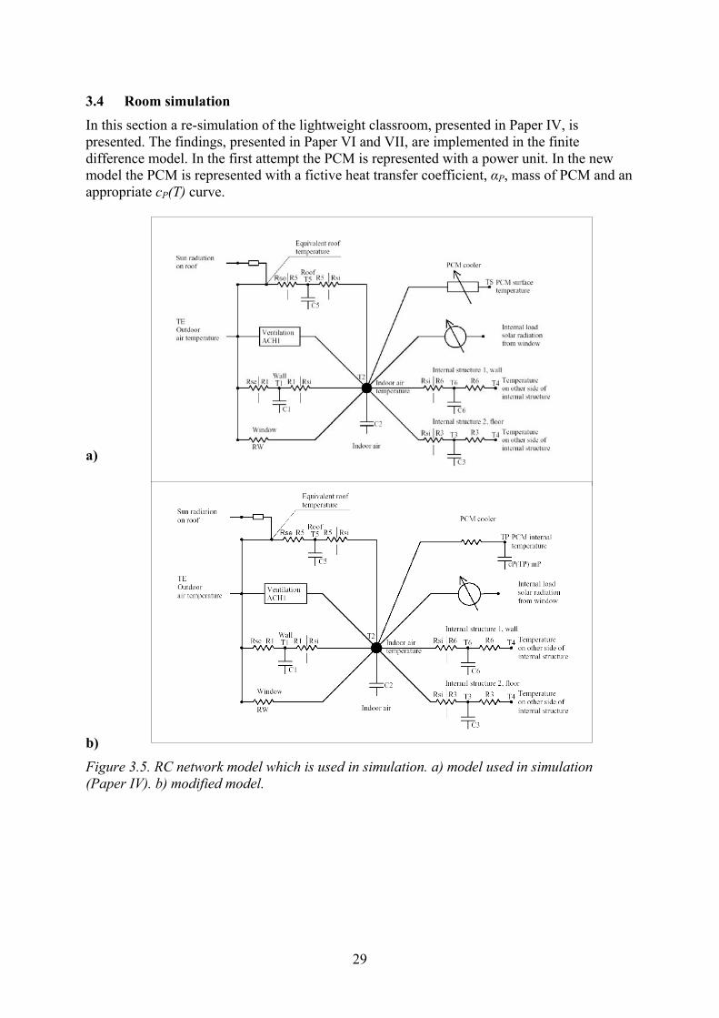
3.4 Room simulation In this section a re-simulation of the lightweight classroom, presented in Paper IV, is presented. The findings, presented in Paper VI and VII, are implemented in the finite difference model. In the first attempt the PCM is represented with a power unit. In the new model the PCM is represented with a fictive heat transfer coefficient, αP, mass of PCM and an appropriate cP(T) curve.

a)

b)

Figure 3.5. RC network model which is used in simulation. a) model used in simulation (Paper IV). b) modified model.

30

3.5 Test of application

3.5.1 Test room

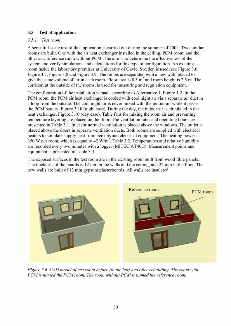
A semi-full-scale test of the application is carried out during the summer of 2004. Two similar rooms are built. One with the air heat exchanger installed in the ceiling, PCM room, and the other as a reference room without PCM. The aim is to determine the effectiveness of the system and verify simulations and calculations for this type of configuration. An existing room inside the laboratory premises at University of Gävle, Sweden is used; see Figure 3.6, Figure 3.7, Figure 3.8 and Figure 3.9. The rooms are separated with a new wall, placed to give the same volume of air in each room. Floor area is 8,3 m2 and room height is 2,5 m. The corridor, at the outside of the rooms, is used for measuring and regulation equipment.

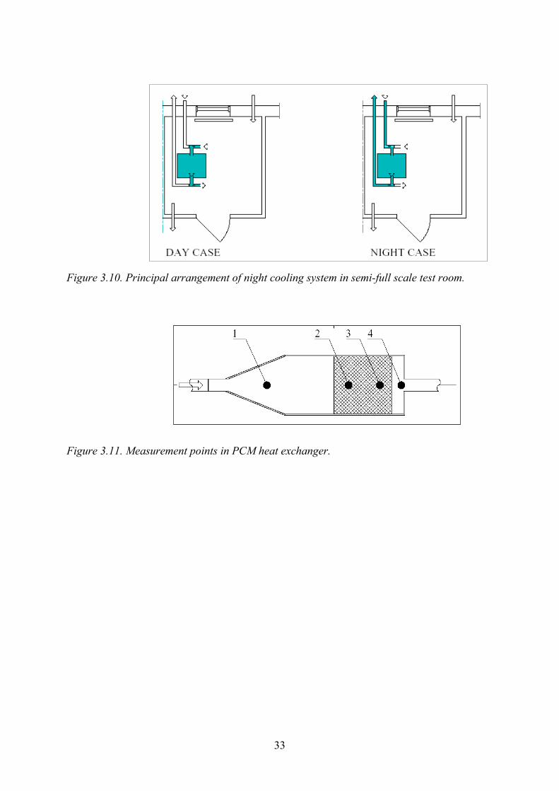
The configuration of the installation is made according to Alternative 1, Figure 1.2. In the PCM room, the PCM air heat exchanger is cooled with cool night air via a separate air duct in a loop from the outside. The cool night air is never mixed with the indoor air while it passes the PCM battery, Figure 3.10 (night case). During the day, the indoor air is circulated in the heat exchanger, Figure 3.10 (day case). Table fans for mixing the room air and preventing temperature layering are placed on the floor. The ventilation rates and operating hours are presented in Table 3.1. Inlet for normal ventilation is placed above the windows. The outlet is placed above the doors in separate ventilation ducts. Both rooms are supplied with electrical heaters to simulate supply heat from persons and electrical equipment. The heating power is 350 W per room, which is equal to 42 W/m2, Table 3.2. Temperatures and relative humidity are recorded every two minutes with a logger (MITEC AT40G). Measurement points and equipment is presented in Table 3.3.

The exposed surfaces in the test room are in the existing room built from wood fibre panels. The thickness of the boards is 12 mm in the walls and the ceiling, and 22 mm in the floor. The new walls are built of 13 mm gypsum plasterboards. All walls are insulated.

Figure 3.6. CAD model of test room before (to the left) and after rebuilding. The room with PCM is named the PCM room. The room without PCM is named the reference room.

Reference room PCM room

31

Table 3.1. Ventilation in PCM room and reference room.

Ventilation Air flow

[m3/s]

Ventilation rate

[hour-1]

On Off

Normal ventilation rate in PCM room and reference room

0,010 1,8

Air flow during day in PCM heat exchanger

0,068 (corresponds to) 13 17.00 08.00

Air flow during night in PCM heat exchanger

0,060 (corresponds to) 12 08.00 17.00

Table 3.2. Scheme for heater in PCM room and reference room.

Power input Power

[W]

On Off

Heater in PCM room and reference room

350 08.00 17.00

Table 3.3. Measurement points and equipment in test room.

Measurement point

Description Equipment Comment

1 Temperature in air inlet of PCM heat exchanger

Termistor (Mitec MU-TE100)

See Figure 3.11

2 Temperature in PCM battery Thermocouple type T See Figure 3.11

3 Temperature in PCM battery Thermocouple type T See Figure 3.11

4 Temperature in air outlet of PCM heat exchanger

Termistor (Mitec MU-TE100)

See Figure 3.11

5 Air temperature in reference room

Thermocouple type T

6 Air temperature in PCM room Thermocouple type T

7 Outdoor air temperature Thermocouple type T

8 Relative humidity in air inlet of PCM heat exchanger

Mitec MU-RV103

32

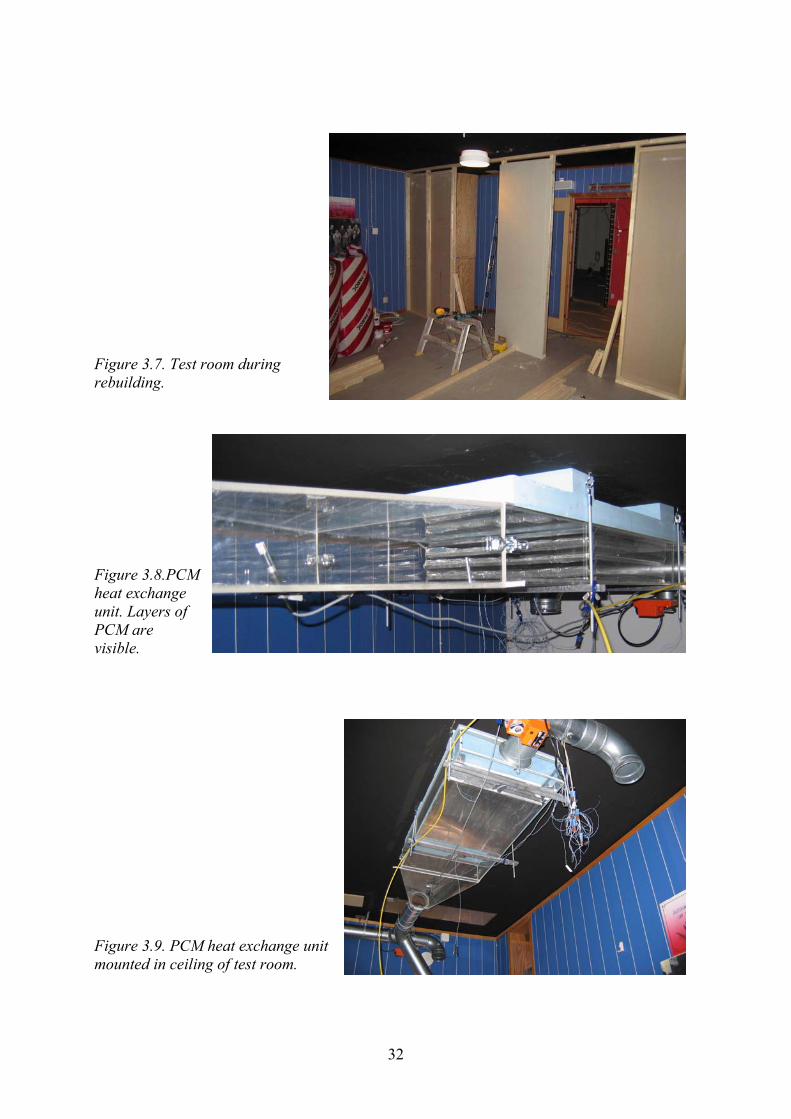
Figure 3.7. Test room during rebuilding.

Figure 3.8.PCM heat exchange unit. Layers of PCM are visible.

Figure 3.9. PCM heat exchange unit mounted in ceiling of test room.

33

Figure 3.10. Principal arrangement of night cooling system in semi-full scale test room.

Figure 3.11. Measurement points in PCM heat exchanger.

34

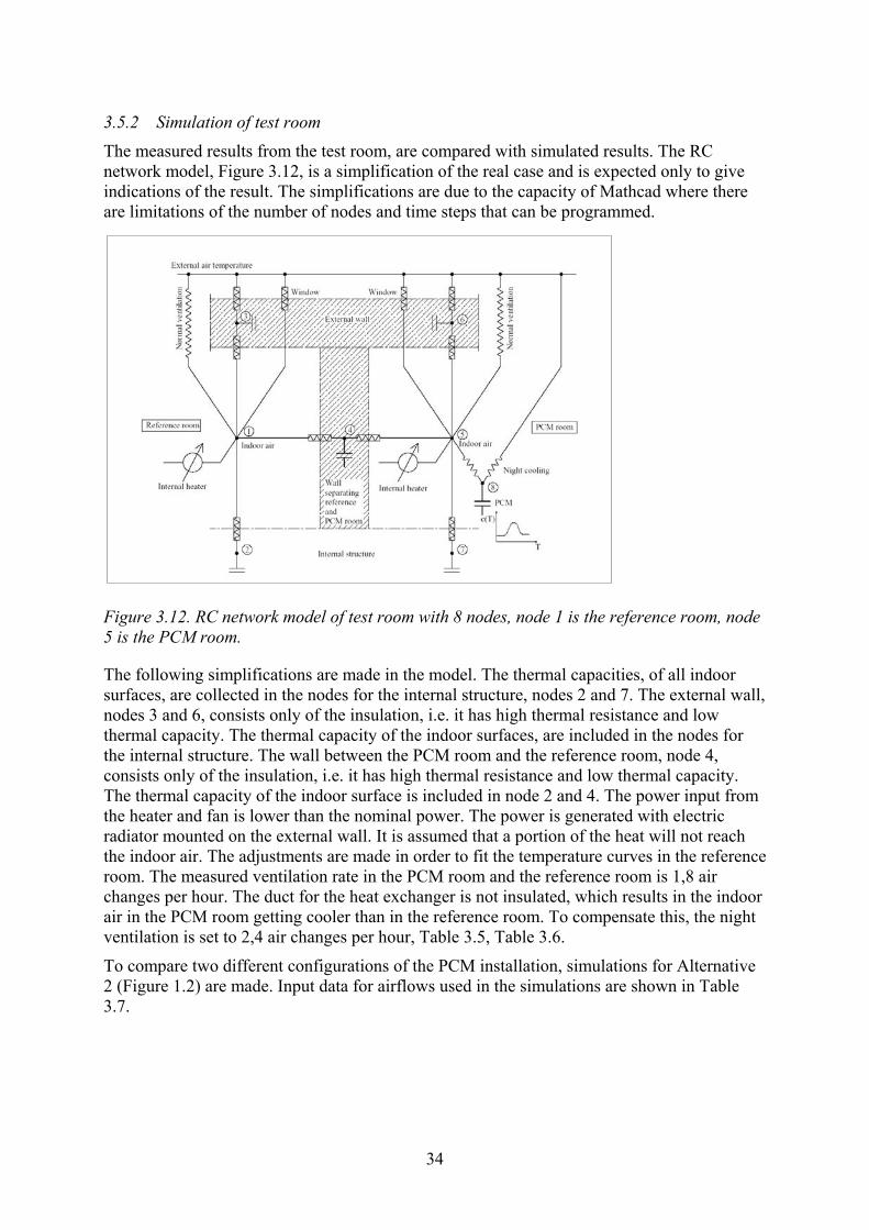
3.5.2 Simulation of test room

The measured results from the test room, are compared with simulated results. The RC network model, Figure 3.12, is a simplification of the real case and is expected only to give indications of the result. The simplifications are due to the capacity of Mathcad where there are limitations of the number of nodes and time steps that can be programmed.

Figure 3.12. RC network model of test room with 8 nodes, node 1 is the reference room, node 5 is the PCM room.

The following simplifications are made in the model. The thermal capacities, of all indoor surfaces, are collected in the nodes for the internal structure, nodes 2 and 7. The external wall, nodes 3 and 6, consists only of the insulation, i.e. it has high thermal resistance and low thermal capacity. The thermal capacity of the indoor surfaces, are included in the nodes for the internal structure. The wall between the PCM room and the reference room, node 4, consists only of the insulation, i.e. it has high thermal resistance and low thermal capacity. The thermal capacity of the indoor surface is included in node 2 and 4. The power input from the heater and fan is lower than the nominal power. The power is generated with electric radiator mounted on the external wall. It is assumed that a portion of the heat will not reach the indoor air. The adjustments are made in order to fit the temperature curves in the reference room. The measured ventilation rate in the PCM room and the reference room is 1,8 air changes per hour. The duct for the heat exchanger is not insulated, which results in the indoor air in the PCM room getting cooler than in the reference room. To compensate this, the night ventilation is set to 2,4 air changes per hour, Table 3.5, Table 3.6.

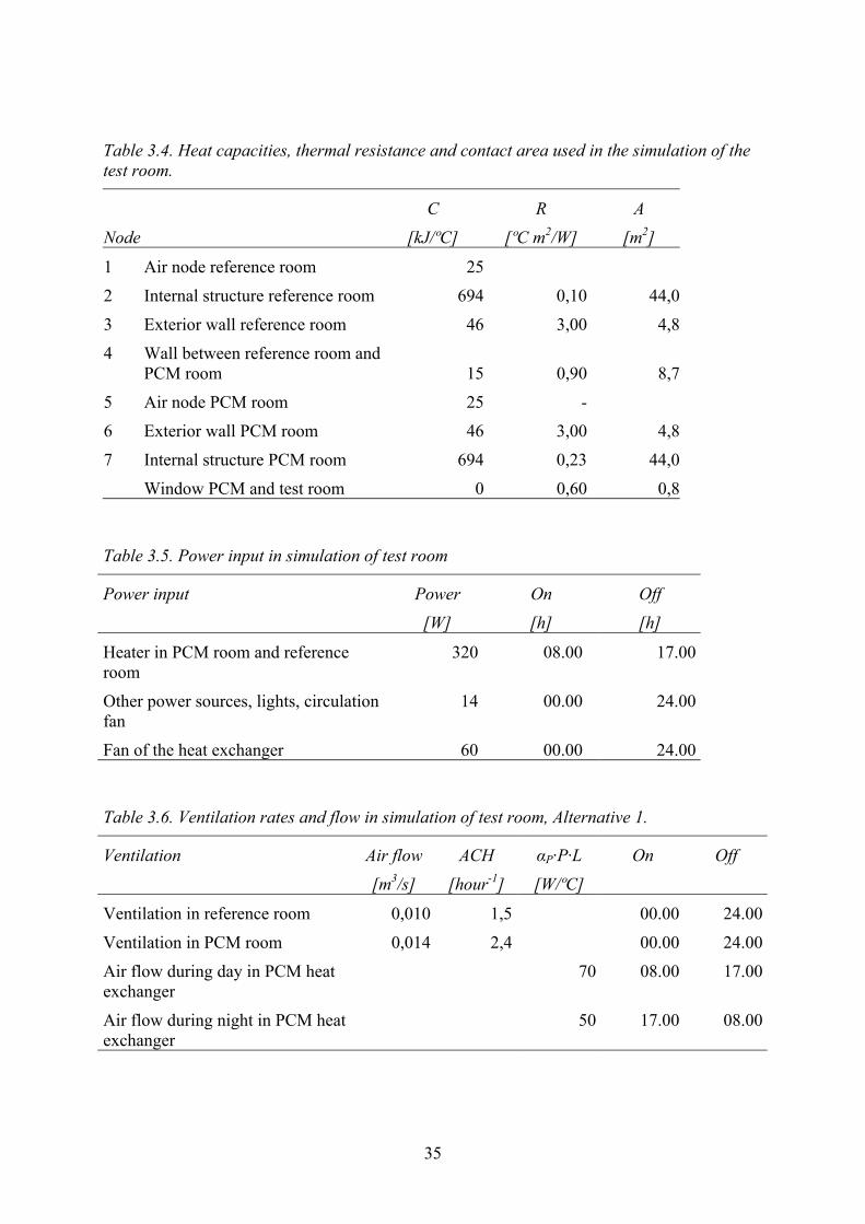
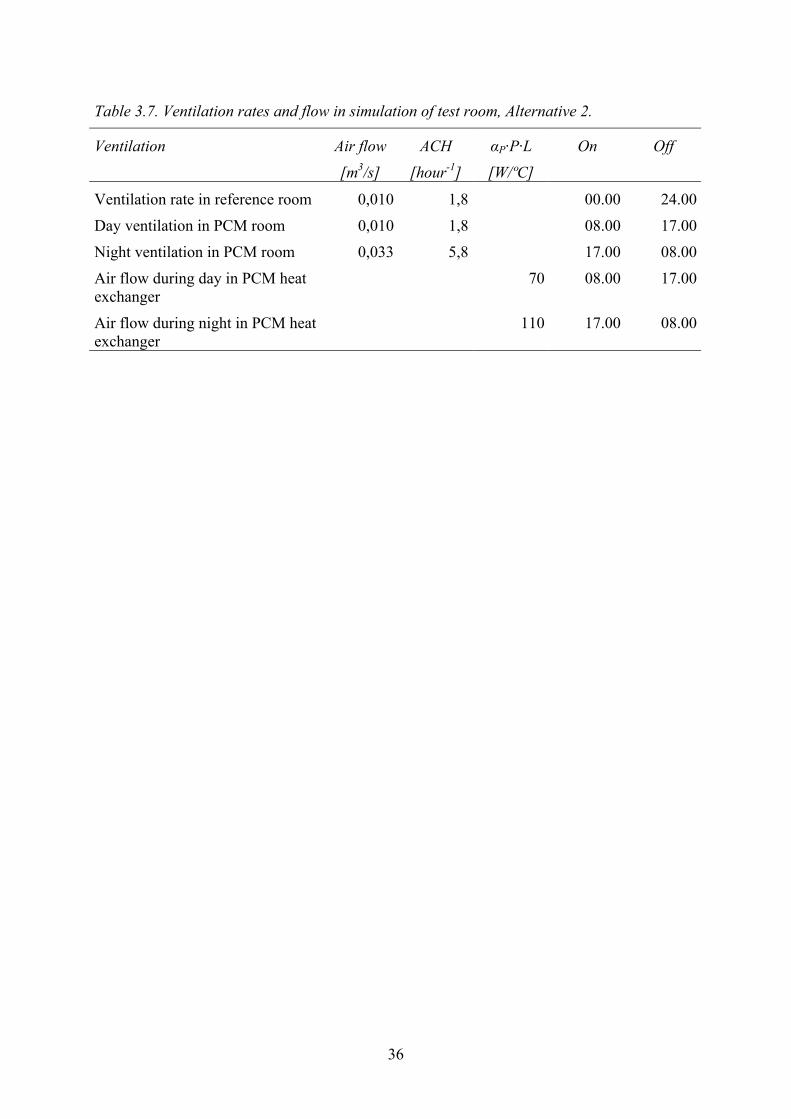
To compare two different configurations of the PCM installation, simulations for Alternative 2 (Figure 1.2) are made. Input data for airflows used in the simulations are shown in Table 3.7.

35

Table 3.4. Heat capacities, thermal resistance and contact area used in the simulation of the test room.

Node

C

[kJ/ºC]

R

[ºC m2/W]

A

[m2]

1 Air node reference room 25

2 Internal structure reference room 694 0,10 44,0

3 Exterior wall reference room 46 3,00 4,8

4 Wall between reference room and PCM room 15 0,90 8,7

5 Air node PCM room 25 -

6 Exterior wall PCM room 46 3,00 4,8

7 Internal structure PCM room 694 0,23 44,0

Window PCM and test room 0 0,60 0,8

Table 3.5. Power input in simulation of test room

Power input Power

[W]

On

[h]

Off

[h]

Heater in PCM room and reference room

320 08.00 17.00

Other power sources, lights, circulation fan

14 00.00 24.00

Fan of the heat exchanger 60 00.00 24.00

Table 3.6. Ventilation rates and flow in simulation of test room, Alternative 1.

Ventilation Air flow

[m3/s]

ACH

[hour-1]

αP·P·L

[W/ºC]

On Off

Ventilation in reference room 0,010 1,5 00.00 24.00

Ventilation in PCM room 0,014 2,4 00.00 24.00

Air flow during day in PCM heat exchanger

70 08.00 17.00

Air flow during night in PCM heat exchanger

50 17.00 08.00

36

Table 3.7. Ventilation rates and flow in simulation of test room, Alternative 2.

Ventilation Air flow

[m3/s]

ACH

[hour-1]

αP·P·L

[W/ºC]

On Off

Ventilation rate in reference room 0,010 1,8 00.00 24.00

Day ventilation in PCM room 0,010 1,8 08.00 17.00

Night ventilation in PCM room 0,033 5,8 17.00 08.00

Air flow during day in PCM heat exchanger

70 08.00 17.00

Air flow during night in PCM heat exchanger

110 17.00 08.00

37

4 RESULTS OF MEASUREMENTS AND SIMULATIONS

4.1 Results of water calorimeter measurements The results from the water calorimeter measurements are presented in Paper VII. Here complementary results are presented.

A summary of the measured values is presented in Table 4.1.

Table 4.1. Results of calorimeter measurements

Temperature range

[ºC]

Average specific heat cAP

[kJ/kg·ºC]

15-45 6,5

18-28 9,7

21-27 9,9

The average specific heat for each sample is presented in Figure 4.3 to Figure 4.8.

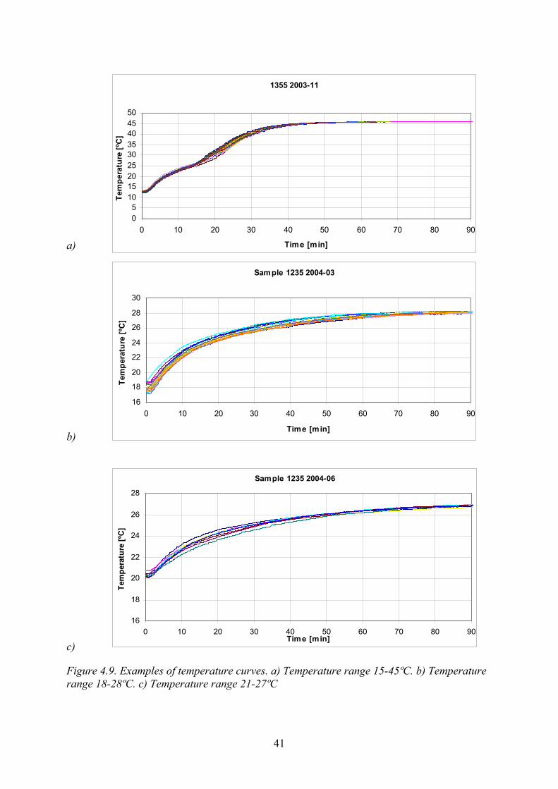
The temperature is measured in the middle of the PCM sample and is recorded every 10 seconds. This results in a band of curves, each representing one measurement. The shape can indicate if there is a phase change, and also at what temperature it takes place. The measured results can also be compared with the simulated result. The curves show only the melting of the PCM. To demonstrate the results of the temperature measurements, representative curves for different samples are shown in Figure 4.9.

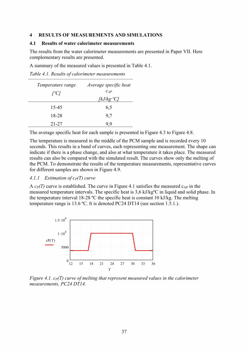
4.1.1 Estimation of cP(T) curve

A cP(T) curve is established. The curve in Figure 4.1 satisfies the measured cAP in the measured temperature intervals. The specific heat is 3,6 kJ/kgºC in liquid and solid phase. In the temperature interval 18-28 ºC the specific heat is constant 10 kJ/kg. The melting temperature range is 13.6 ºC. It is denoted PC24 DT14 (see section 1.5.1.).

Figure 4.1. cP(T) curve of melting that represent measured values in the calorimeter measurements, PC24 DT14.

12 15 18 21 24 27 30 33 360

5000

1 .104

1.5 .104

cP T( )

T

38

1235 2004-03 (18-28)

16

18

20

22

24

26

28

30

0 10 20 30 40 50 60 70 80 90

Time [min]

Tem

pera

ture

[ºC

]

Simulated curve

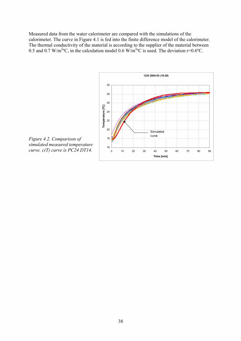
Measured data from the water calorimeter are compared with the simulations of the calorimeter. The curve in Figure 4.1 is fed into the finite difference model of the calorimeter. The thermal conductivity of the material is according to the supplier of the material between 0.5 and 0.7 W/m2ºC, in the calculation model 0.6 W/m2ºC is used. The deviation r=0.6ºC.

Figure 4.2. Comparison of simulated measured temperature curve. c(T) curve is PC24 DT14.

39

Sample 1235

-

2

4

6

8

10

12

14

16

03-09-15

03-10-13

03-11-10

03-12-08

04-01-05

04-02-02

04-03-01

04-03-29

04-04-26

04-05-24

04-06-21

04-07-19

04-08-16

04-09-13

Date

c AP

[kJ/

kgºC

]

cAP 15-45 cAP 18-28 cAP 21-27

Sample 1355

-

2

4

6

8

10

12

14

16

03-09-15

03-10-13

03-11-10

03-12-08

04-01-05

04-02-02

04-03-01

04-03-29

04-04-26

04-05-24

04-06-21

04-07-19

04-08-16

04-09-13

Date

c AP

[kJ/

kgºC

]

cAP 15-45 cAP 18-28 cAP 21-27

Sample 1435

-

2

4

6

8

10

12

14

16

03-09-15

03-10-13

03-11-10

03-12-08

04-01-05

04-02-02

04-03-01

04-03-29

04-04-26

04-05-24

04-06-21

04-07-19

04-08-16

04-09-13

Date

c AP [k

J/kg

ºC]

cAP 15-45 cAP 18-28 cAP 21-27

Figure 4.3. Results of water calorimeter measurements for temperature sample 1235.

Figure 4.4. Results of water calorimeter measurements for sample 1355.

Figure 4.5. Results of water calorimeter measurements for sample 1435.

40

Sample 1577

-

2

4

6

8

10

12

14

16

03-09-15

03-10-13

03-11-10

03-12-08

04-01-05

04-02-02

04-03-01

04-03-29

04-04-26

04-05-24

04-06-21

04-07-19

04-08-16

04-09-13

c AP [k

J/kg

ºC]

cAP 15-45 cAP 18-28 cAP 21-27

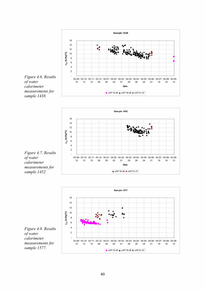
Figure 4.6. Results of water calorimeter measurements for sample 1438.

Figure 4.7. Results of water calorimeter measurements for sample 1452.

Figure 4.8. Results of water calorimeter measurements for sample 1577.

Sample 1438

-

2

4

6

8

10

12

14

16

03-09-15

03-10-13

03-11-10

03-12-08

04-01-05

04-02-02

04-03-01

04-03-29

04-04-26

04-05-24

04-06-21

04-07-19

04-08-16

04-09-13

Date

c AP [k

J/kg

ºC]

cAP 15-45 cAP 18-28 cAP 21-27

Sample 1452

-

2

4

6

8

10

12

14

16

03-09-15

03-10-13

03-11-10

03-12-08

04-01-05

04-02-02

04-03-01

04-03-29

04-04-26

04-05-24

04-06-21

04-07-19

04-08-16

04-09-13

Date

c AP [k

J/kg

ºC]

cAP 18-28 cAP 21-27

41

a)

b)

c)

Figure 4.9. Examples of temperature curves. a) Temperature range 15-45ºC. b) Temperature range 18-28ºC. c) Temperature range 21-27ºC

1355 2003-11

05

101520253035404550

0 10 20 30 40 50 60 70 80 90

Time [min]

Tem

pera

ture

[ºC

]

Sample 1235 2004-03

16

18

20

22

24

26

28

30

0 10 20 30 40 50 60 70 80 90

Time [min]

Tem

pera

ture

[ºC

]

Sample 1235 2004-06

16

18

20

22

24

26

28

0 10 20 30 40 50 60 70 80 90Time [min]

Tem

pera

ture

[ºC

]

42

4.2 Air heat exchanger

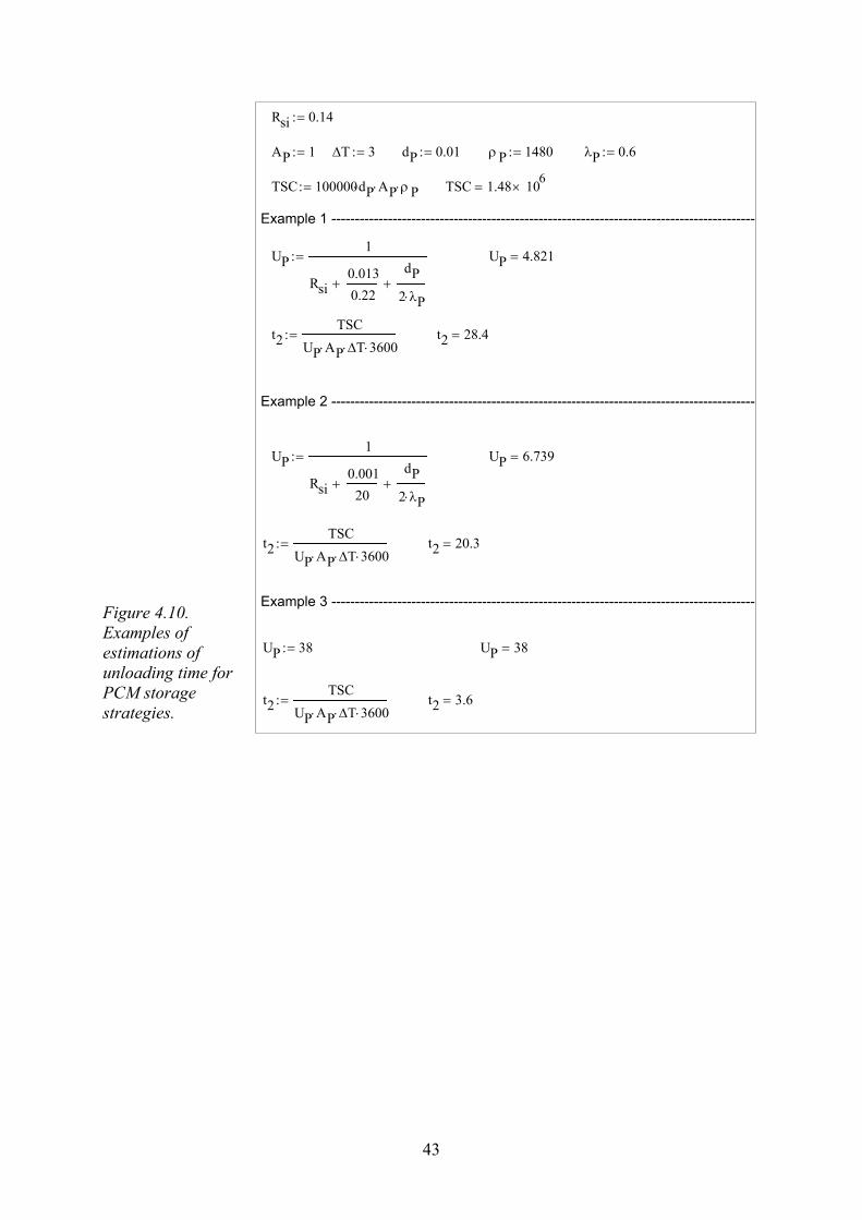
4.2.1 Comparison between natural convection and heat exchanger

If the PCM is stored behind the surface material in a wall, floor or ceiling, the energy exchange between the PCM and the ambient air takes place with natural convection. Expression [3.20] can be written:

( )Pr TTAUq −⋅⋅=

Where

∑++=

iPsi RRRU 1

where Rsi is the heat transfer coefficient between the indoor air and an indoor surface.

The energy that can be stored or released from time t1 to t2 is

∫ ⋅−⋅⋅=2

1

)(t

tPr dtTTAUTSC

If UP and A are constant, the temperature difference (Tr-TP) is assumed to 3 ºC, and the starting time is 0, an estimation of the unloading time (during night) for different cases can be done. The unloading time can be estimated to

)(2Pr TTAU

TSCt−⋅⋅

=

The actual heat exchanger has rough surface and the fictive heat transfer coefficient is calculated to 38 W/m2ºC. Assume the latent heat of the PCM is 100 000 J/kg. The thickness of the PCM is 0.01 m and the density is 1480 kg/m3. For 1 m2 the unloading time is estimated for three examples.

Example 1: PCM is stored behind 13 mm gypsum board.

Example 2: PCM is stored behind a metal sheet.

Example 3: PCM is stored in heat exchanger.

The estimated unloading times are approximately 27, 19 and 3.5 hours. This shows that there could be difficulties in unloading a PCM storage with natural convection, Figure 4.10.

43

t2 3.6=t2TSC

UP AP⋅ ∆T⋅ 3600⋅:=

UP 38=UP 38:=

Example 3 ------------------------------------------------------------------------------------------

t2 20.3=t2TSC

UP AP⋅ ∆T⋅ 3600⋅:=

UP 6.739=UP1

Rsi0.001

20+

dP2 λP⋅

+

:=

Example 2 ------------------------------------------------------------------------------------------

t2 28.4=t2TSC

UP AP⋅ ∆T⋅ 3600⋅:=

UP 4.821=UP1

Rsi0.0130.22

+dP

2 λP⋅+

:=

Example 1 ------------------------------------------------------------------------------------------

TSC 1.48 106×=TSC 100000dP⋅ AP⋅ ρ P⋅:=

λP 0.6:=ρ P 1480:=dP 0.01:=∆T 3:=AP 1:=

Rsi 0.14:=

Figure 4.10. Examples of estimations of unloading time for PCM storage strategies.

44

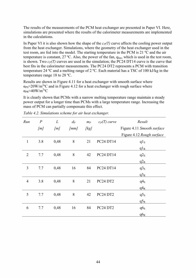
The results of the measurements of the PCM heat exchanger are presented in Paper VI. Here, simulations are presented where the results of the calorimeter measurements are implemented in the calculations.

In Paper VI it is also shown how the shape of the cP(T) curve affects the cooling power output from the heat exchanger. Simulations, where the geometry of the heat exchanger used in the test room, are fed into the model. The starting temperature in the PCM is 21 ºC and the air temperature is constant, 27 ºC. Also, the power of the fan, qfan, which is used in the test room, is shown. Two cP(T) curves are used in the simulation; the PC24 DT14 curve is the curve that best fits in the calorimeter measurements. The PC24 DT2 represents a PCM with transition temperature 24 ºC and a melting range of 2 ºC. Each material has a TSC of 100 kJ/kg in the temperature range 18 to 28 ºC.

Results are shown in Figure 4.11 for a heat exchanger with smooth surface where αPS≈20W/m2ºC and in Figure 4.12 for a heat exchanger with rough surface where αPR≈40W/m2ºC

It is clearly shown that PCMs with a narrow melting temperature range maintain a steady power output for a longer time than PCMs with a large temperature range. Increasing the mass of PCM can partially compensate this effect.

Table 4.2. Simulations scheme for air heat exchanger.

Run P

[m]

L

[m]

dP

[mm]

mP

[kg]

cP(T) curve Result

Figure 4.11 Smooth surface

Figure 4.12 Rough surface

1 3.8 0,48 8 21 PC24 DT14 q1S

q1R

2 7.7 0,48 8 42 PC24 DT14 q2S

q2R

3 7.7 0,48 16 84 PC24 DT14 q3S

q3R

4 3.8 0,48 8 21 PC24 DT2 q4S

q4R

5 7.7 0,48 8 42 PC24 DT2 q5S

q5R

6 7.7 0,48 16 84 PC24 DT2 q6S

q6R

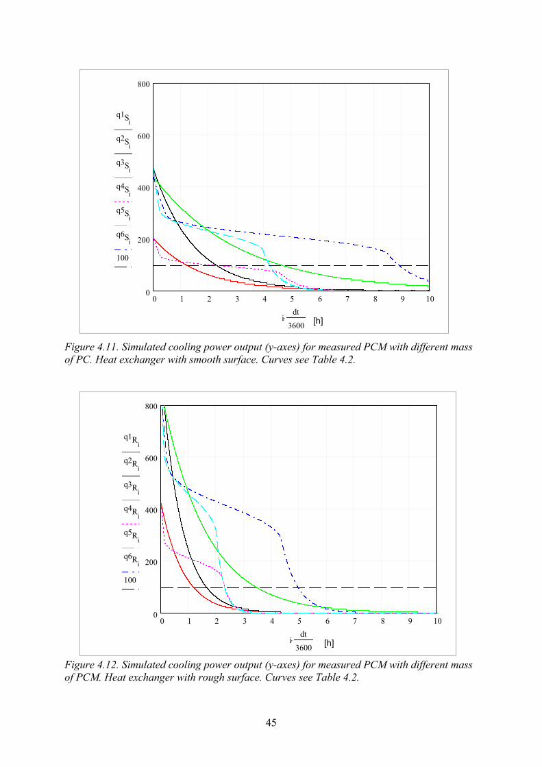
45

Figure 4.11. Simulated cooling power output (y-axes) for measured PCM with different mass of PC. Heat exchanger with smooth surface. Curves see Table 4.2.

Figure 4.12. Simulated cooling power output (y-axes) for measured PCM with different mass of PCM. Heat exchanger with rough surface. Curves see Table 4.2.

0 1 2 3 4 5 6 7 8 9 100

200

400

600

800

q1Ri

q2Ri

q3Ri

q4Ri

q5Ri

q6Ri

100

idt

3600⋅ [h]

0 1 2 3 4 5 6 7 8 9 100

200

400

600

800

q1Si

q2Si

q3Si

q4Si

q5Si

q6Si

100

idt

3600⋅ [h]

46

4.3 Room simulation The modified calculation model is implemented in the simulation model for building B11. The floor area is 60 m2 and the air volume 180 m3. The simulations are made for the case shown in Figure 4.13, where only the indoor air is circulated in the PCM storage. The night ventilation is forced.

Figure 4.13. Principal arrangement of night cooling system in the room simulations.

The results are compared with the results from Paper IV. Simulations are made for the measured PCM where DT=14 and for a desired PCM where DT=2 ºC. The following runs are made, see Table 4.3.

Table 4.3. Program for room simulations with different configurations of PCM.

Run Mass

[kg/m2]

αP·P·L

day/night

[W/ºC]

cP(T) Curve

1 No PCM 0 - No PCM

2 PCM modelled as power unit

3,5

0 PCM-power-un

3 PCM, latent heat 3,5 413/510 PC24 DT2

4 7,0 413/510 PC24 DT2

5 14,0 413/510 PC24 DT2

6 Measured material 3,5 413/510 PC24 DT14

7 7,0 413/510 PC24 DT14

8 14,0 413/510 PC24 DT14

47

In Paper IV, the PCM heat exchanger is modelled as a power unit. This corresponds to a PCM with narrow melting temperature range. The simulated indoor air temperatures are compared for daytime during day 9, Figure 4.14 and Figure 4.15. The shape of the PC24 DT2(3,5) curve indicates that the amount of PCM is not sufficient for the actual thermal load. All PCM is melted. The shapes of the other curves are similar for both models. That indicates that an ideal PCM with a low DT, i.e. near isothermal melting, will act as a power unit with constant power.

The goal can be set as maximum allowable time for a certain room air temperature. The temperature distribution can be expressed with a cumulative frequency curve. An example of this is shown in Figure 4.18. If temperatures above 27 ºC should be avoided for approximately 5% of the total time, 3,5 kg/m2 of PC24 DT2 is needed. For a PC24 DT14, the double amount is needed. The conclusion is: To achieve the same results as in Paper IV, two to four times the amounts suggested will be necessary to install in the building.

48

15

20

25

30

06:00 08:00 10:00 12:00 14:00 16:00 18:00

Time [h]

Tem

pera

ture

[ºC

]

NoPCM Paper 1 PC24 DT2(3,5) PC24 DT14(3,5)

Figure 4.14. Comparison of simulated indoor air temperatures for day 14. Mass PCM=3,5 kg/m2

Figure 4.15. Comparison of simulated indoor air temperatures for day 14. Mass PCM=7 kg/m2.

Figure 4.16. Comparison of simulated indoor air temperatures for day 14. Mass PCM=14 kg/m2.

15

20

25

30

06:00 08:00 10:00 12:00 14:00 16:00 18:00

Time [h]

Tem

pera

ture

[ºC

]

NoPCM Paper 1 PC24 DT2(7) PC24 DT14(7)

15

20

25

30

06:00 08:00 10:00 12:00 14:00 16:00 18:00

Time [h]

Tem

pera

ture

[ºC

]

NoPCM Paper 1 PC24 DT2(14) PC24 DT14(14)

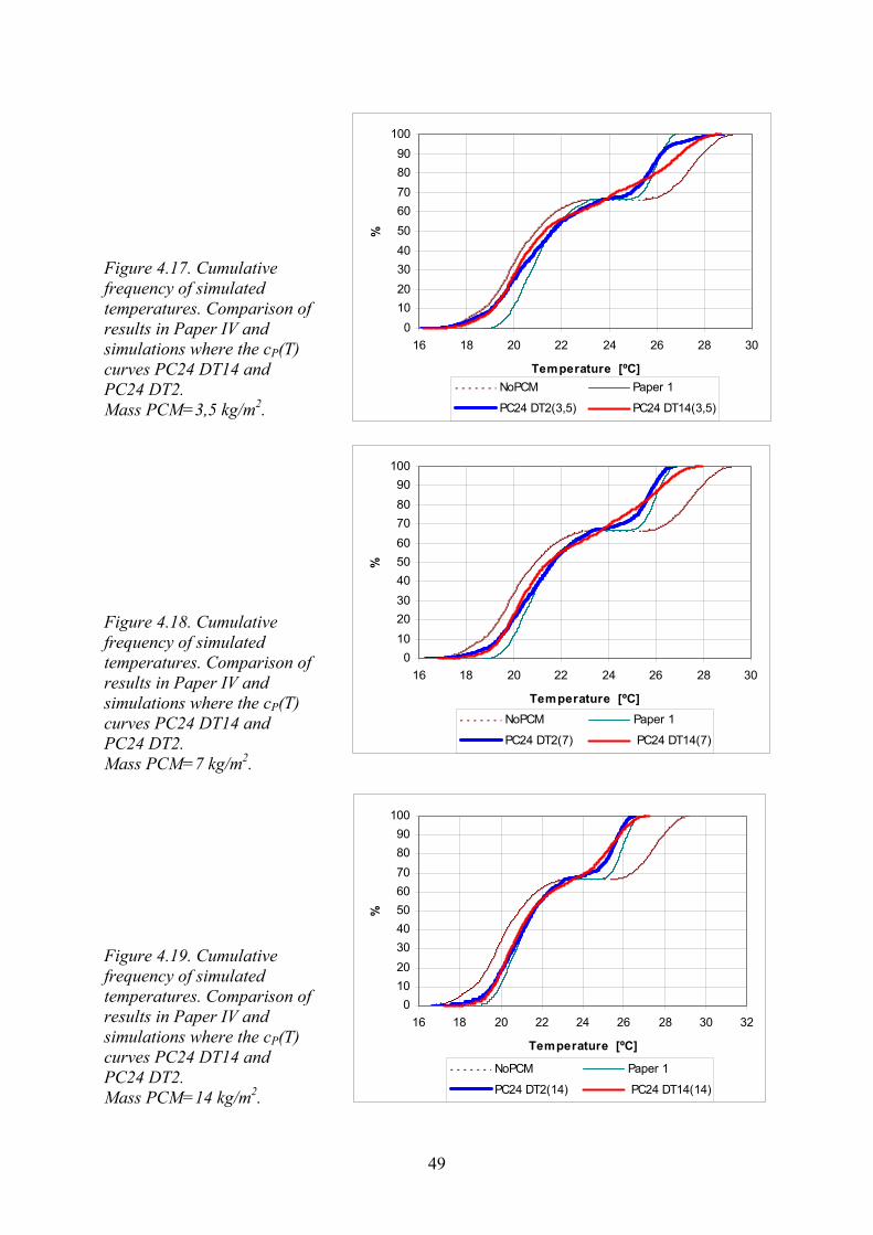
49

Figure 4.17. Cumulative frequency of simulated temperatures. Comparison of results in Paper IV and simulations where the cP(T) curves PC24 DT14 and PC24 DT2. Mass PCM=3,5 kg/m2.

Figure 4.18. Cumulative frequency of simulated temperatures. Comparison of results in Paper IV and simulations where the cP(T) curves PC24 DT14 and PC24 DT2. Mass PCM=7 kg/m2.

Figure 4.19. Cumulative frequency of simulated temperatures. Comparison of results in Paper IV and simulations where the cP(T) curves PC24 DT14 and PC24 DT2. Mass PCM=14 kg/m2.

0102030405060708090

100

16 18 20 22 24 26 28 30

Temperature [ºC]%

NoPCM Paper 1

PC24 DT2(3,5) PC24 DT14(3,5)

0102030405060708090

100

16 18 20 22 24 26 28 30

Temperature [ºC]

%

NoPCM Paper 1

PC24 DT2(7) PC24 DT14(7)

0102030405060708090

100

16 18 20 22 24 26 28 30 32

Temperature [ºC]

%

NoPCM Paper 1

PC24 DT2(14) PC24 DT14(14)

50

4.4 Results of temperature measurements and simulations in test room

4.4.1 Room air temperatures

A distribution of the room air temperatures during 56-days of measuring is shown in Figure 4.20. It starts at 2004-06-28, day 56 is 2004-08-22. Temperatures for five days are shown from the measurements, Figure 4.21.

Figure 4.20. Cumulative frequency of measured temperatures in PCM room and reference room during a 56-day period from 2004-06-28.

Figure 4.21. Measured temperatures from 2004-07-01 to 2004-07-05 in test room.

10 12 14 16 18 20 22 24 26 28 30 32 34

04-07-01 04-07-02 04-07-03 04-07-04 04-07-05

Date

Tem

pera

ture

[ºC

]

Outdoor PCM room Reference room PCM outlet

Outdoor

Reference room

PCM room

PCM

- 10 20 30 40 50 60 70 80 90

100

15 18 21 24 27 30 33 36

Temperature [ºC]

%

PCM room Reference room

51

It is noted that there is a lower temperature in the PCM room during the day, and much lower during night. The pattern of the day temperature measurements show that in the beginning of the daytime measurements at 08.00, the temperature difference is about 2 ºC, and at the end of the daytime, at 20.00, there is no temperature difference. During night the duct that leads the cool night air into the room will have a cooling effect on the entire room.

The measured temperatures are compared with the simulated temperatures. For day 7 to 14 the temperatures in the reference room are shown in Figure 4.22, and in the PCM room in Figure 4.23. The deviation between the measured and simulated temperatures is shown in Table 4.4.

Figure 4.22. Measured (RRm(t·dt)) and simulated (T1,t) temperatures from day 7 to 14 in the reference room (2004-07-10 to 2004-07-17).

Figure 4.23. Measured (TRm(t·dt)) and simulated (T5,t) temperatures from day 7 to 14 in the PCM room (2004-07-10 to 2004-07-17)..

7 8 9 10 11 12 13 141617181920212223242526272829303132

T5 t,

TRm t dt⋅( )

t dt⋅

24 3600⋅

7 8 9 10 11 12 13 141617181920212223242526272829303132

T1 t,

RRm t dt⋅( )

t dt⋅

24 3600⋅

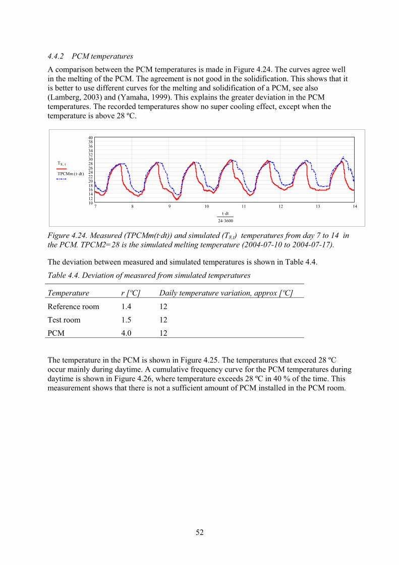
52

4.4.2 PCM temperatures

A comparison between the PCM temperatures is made in Figure 4.24. The curves agree well in the melting of the PCM. The agreement is not good in the solidification. This shows that it is better to use different curves for the melting and solidification of a PCM, see also (Lamberg, 2003) and (Yamaha, 1999). This explains the greater deviation in the PCM temperatures. The recorded temperatures show no super cooling effect, except when the temperature is above 28 ºC.

Figure 4.24. Measured (TPCMm(t·dt)) and simulated (T8,t) temperatures from day 7 to 14 in the PCM. TPCM2=28 is the simulated melting temperature (2004-07-10 to 2004-07-17).

The deviation between measured and simulated temperatures is shown in Table 4.4.

Table 4.4. Deviation of measured from simulated temperatures

Temperature r [ºC] Daily temperature variation, approx [ºC]

Reference room 1.4 12

Test room 1.5 12

PCM 4.0 12

The temperature in the PCM is shown in Figure 4.25. The temperatures that exceed 28 ºC occur mainly during daytime. A cumulative frequency curve for the PCM temperatures during daytime is shown in Figure 4.26, where temperature exceeds 28 ºC in 40 % of the time. This measurement shows that there is not a sufficient amount of PCM installed in the PCM room.

7 8 9 10 11 12 13 1410121416182022242628303234363840

T8 t,

TPCMm t dt⋅( )

t dt⋅

24 3600⋅

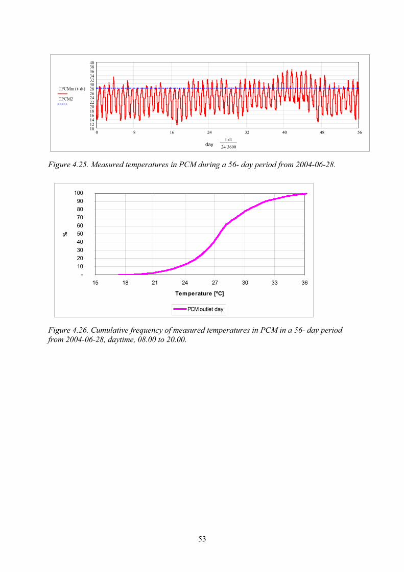
53

Figure 4.25. Measured temperatures in PCM during a 56- day period from 2004-06-28.

Figure 4.26. Cumulative frequency of measured temperatures in PCM in a 56- day period from 2004-06-28, daytime, 08.00 to 20.00.

0 8 16 24 32 40 48 5610121416182022242628303234363840

TPCMm t dt⋅( )

TPCM2

t dt⋅

24 3600⋅day

- 10 20 30 40 50 60 70 80 90

100

15 18 21 24 27 30 33 36

Temperature [ºC]

%

PCM outlet day

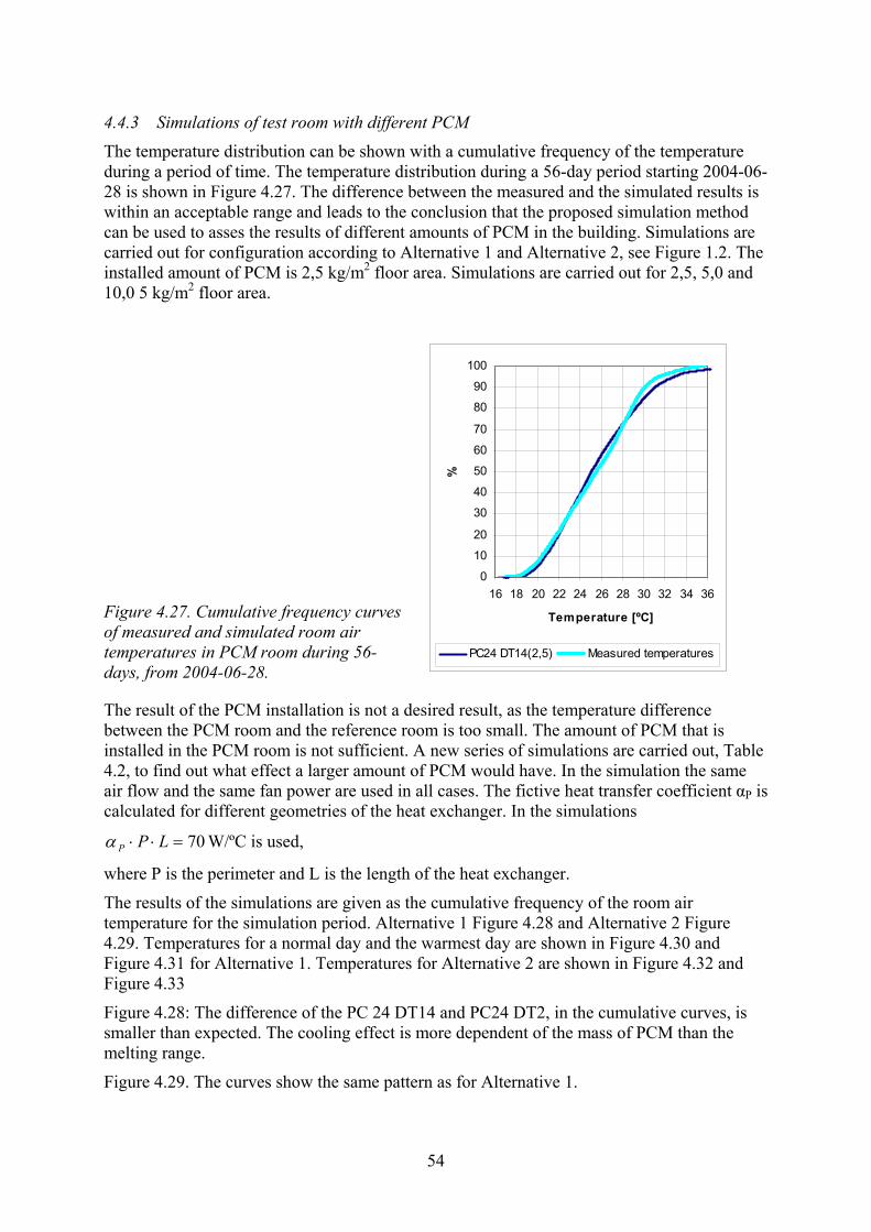
54

0

10

20

30

40

50

60

70

80

90

100

16 18 20 22 24 26 28 30 32 34 36

Temperature [ºC]

%

PC24 DT14(2,5) Measured temperatures

4.4.3 Simulations of test room with different PCM

The temperature distribution can be shown with a cumulative frequency of the temperature during a period of time. The temperature distribution during a 56-day period starting 2004-06-28 is shown in Figure 4.27. The difference between the measured and the simulated results is within an acceptable range and leads to the conclusion that the proposed simulation method can be used to asses the results of different amounts of PCM in the building. Simulations are carried out for configuration according to Alternative 1 and Alternative 2, see Figure 1.2. The installed amount of PCM is 2,5 kg/m2 floor area. Simulations are carried out for 2,5, 5,0 and 10,0 5 kg/m2 floor area.

Figure 4.27. Cumulative frequency curves of measured and simulated room air temperatures in PCM room during 56-days, from 2004-06-28.

The result of the PCM installation is not a desired result, as the temperature difference between the PCM room and the reference room is too small. The amount of PCM that is installed in the PCM room is not sufficient. A new series of simulations are carried out, Table 4.2, to find out what effect a larger amount of PCM would have. In the simulation the same air flow and the same fan power are used in all cases. The fictive heat transfer coefficient αP is calculated for different geometries of the heat exchanger. In the simulations

70=⋅⋅ LPPα W/ºC is used,

where P is the perimeter and L is the length of the heat exchanger.

The results of the simulations are given as the cumulative frequency of the room air temperature for the simulation period. Alternative 1 Figure 4.28 and Alternative 2 Figure 4.29. Temperatures for a normal day and the warmest day are shown in Figure 4.30 and Figure 4.31 for Alternative 1. Temperatures for Alternative 2 are shown in Figure 4.32 and Figure 4.33

Figure 4.28: The difference of the PC 24 DT14 and PC24 DT2, in the cumulative curves, is smaller than expected. The cooling effect is more dependent of the mass of PCM than the melting range.

Figure 4.29. The curves show the same pattern as for Alternative 1.

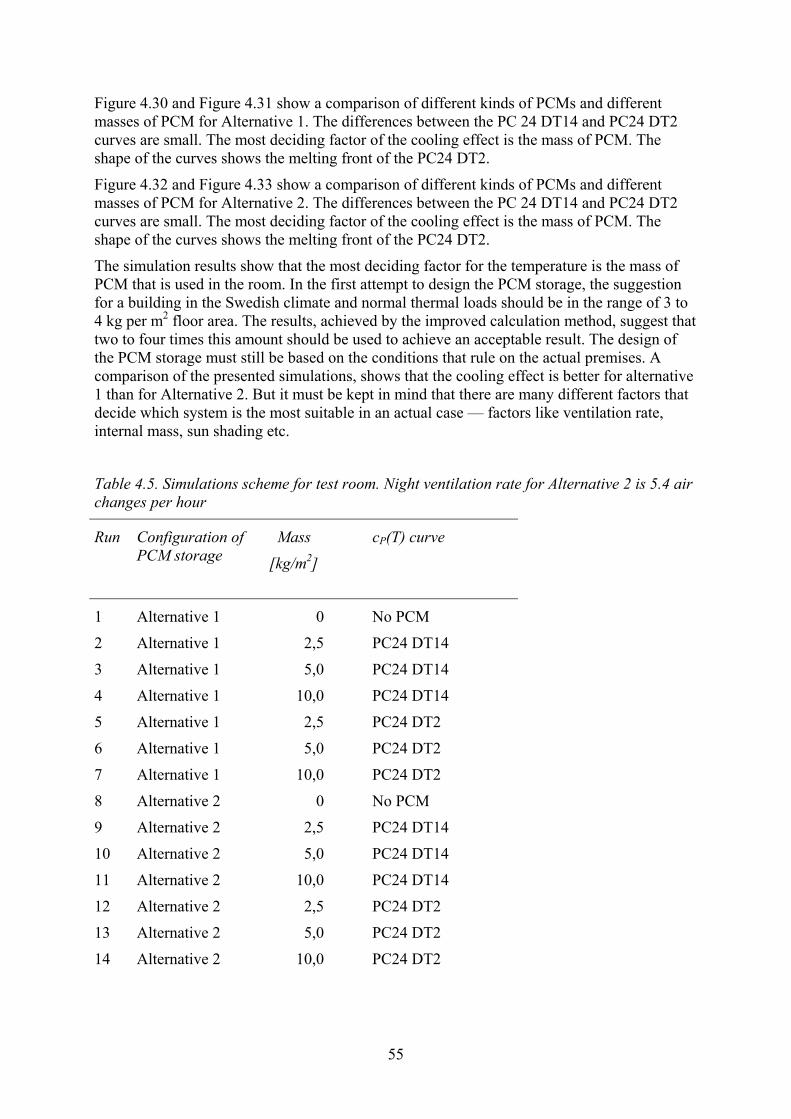
55

Figure 4.30 and Figure 4.31 show a comparison of different kinds of PCMs and different masses of PCM for Alternative 1. The differences between the PC 24 DT14 and PC24 DT2 curves are small. The most deciding factor of the cooling effect is the mass of PCM. The shape of the curves shows the melting front of the PC24 DT2.

Figure 4.32 and Figure 4.33 show a comparison of different kinds of PCMs and different masses of PCM for Alternative 2. The differences between the PC 24 DT14 and PC24 DT2 curves are small. The most deciding factor of the cooling effect is the mass of PCM. The shape of the curves shows the melting front of the PC24 DT2.

The simulation results show that the most deciding factor for the temperature is the mass of PCM that is used in the room. In the first attempt to design the PCM storage, the suggestion for a building in the Swedish climate and normal thermal loads should be in the range of 3 to 4 kg per m2 floor area. The results, achieved by the improved calculation method, suggest that two to four times this amount should be used to achieve an acceptable result. The design of the PCM storage must still be based on the conditions that rule on the actual premises. A comparison of the presented simulations, shows that the cooling effect is better for alternative 1 than for Alternative 2. But it must be kept in mind that there are many different factors that decide which system is the most suitable in an actual case — factors like ventilation rate, internal mass, sun shading etc.

Table 4.5. Simulations scheme for test room. Night ventilation rate for Alternative 2 is 5.4 air changes per hour

Run Configuration of PCM storage

Mass

[kg/m2]

cP(T) curve

1 Alternative 1 0 No PCM

2 Alternative 1 2,5 PC24 DT14

3 Alternative 1 5,0 PC24 DT14

4 Alternative 1 10,0 PC24 DT14

5 Alternative 1 2,5 PC24 DT2

6 Alternative 1 5,0 PC24 DT2

7 Alternative 1 10,0 PC24 DT2

8 Alternative 2 0 No PCM

9 Alternative 2 2,5 PC24 DT14

10 Alternative 2 5,0 PC24 DT14

11 Alternative 2 10,0 PC24 DT14

12 Alternative 2 2,5 PC24 DT2

13 Alternative 2 5,0 PC24 DT2

14 Alternative 2 10,0 PC24 DT2

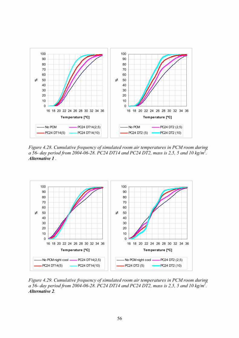
56

Figure 4.28. Cumulative frequency of simulated room air temperatures in PCM room during a 56- day period from 2004-06-28. PC24 DT14 and PC24 DT2, mass is 2,5, 5 and 10 kg/m2. Alternative 1 .

Figure 4.29. Cumulative frequency of simulated room air temperatures in PCM room during a 56- day period from 2004-06-28. PC24 DT14 and PC24 DT2, mass is 2,5, 5 and 10 kg/m2. Alternative 2.

0102030405060708090

100

16 18 20 22 24 26 28 30 32 34 36

Temperature [ºC]

%

No PCM night cool PC24 DT14(2,5)

PC24 DT14(5) PC24 DT14(10)

0102030405060708090

100

16 18 20 22 24 26 28 30 32 34 36

Temperature [ºC]

%

No PCM night cool PC24 DT2 (2,5)

PC24 DT2 (5) PC24 DT2 (10)

0102030405060708090

100

16 18 20 22 24 26 28 30 32 34 36

Temperature [ºC]

%

No PCM PC24 DT14(2,5)

PC24 DT14(5) PC24 DT14(10)

0102030405060708090

100

16 18 20 22 24 26 28 30 32 34 36

Temperature [ºC]%

No PCM PC24 DT2 (2,5)

PC24 DT2 (5) PC24 DT2 (10)

57

18192021222324252627282930313233343536373839404142

06:00 12:00 18:00

Time [h] Day 9

Tem

pera

ture

[ºC

]

No PCM PC24 DT14(10)

PC24 DT2 (10)

18192021222324252627282930313233343536373839404142

06:00 12:00 18:00

Time [h] Day 9

Tem

pera

ture

[ºC

]

No PCM PC24 DT14(5)

PC24 DT2 (5)

18192021222324252627282930313233343536373839404142

06:00 12:00 18:00

Time [h] Day 9

Tem

pera

ture

[ºC

]

No PCM PC24 DT14(2,5)

PC24 DT2 (2,5)

18192021222324252627282930313233343536373839404142

06:00 12:00 18:00

Time [h] Day 40

Tem

pera

ture

[ºC

]

No PCM PC24 DT14(5)

PC24 DT2 (5)

18192021222324252627282930313233343536373839404142

06:00 12:00 18:00

Time [h] Day 40

Tem

pera

ture

[ºC

]

No PCM PC24 DT14(2,5)

PC24 DT2 (2,5)

18192021222324252627282930313233343536373839404142

06:00 12:00 18:00

Time [h] Day 40

Tem

pera

ture

[ºC

]

No PCM PC24 DT14(10)

PC24 DT2 (10)

Figure 4.30. Simulated room air temperatures in PCM room a normal day (day 9) PCM mass are 2,5, 5 and 10 kg/m2 floor area. Comparison for PC24 DT14 and PC24 DT2. Alternative 1.

Figure 4.31. Simulated room air temperatures in PCM room the warmest day (day40) PCM mass are 2,5, 5 and 10 kg/m2 floor area. Comparison for PC24 DT14 and PC24 DT2. Alternative 1.

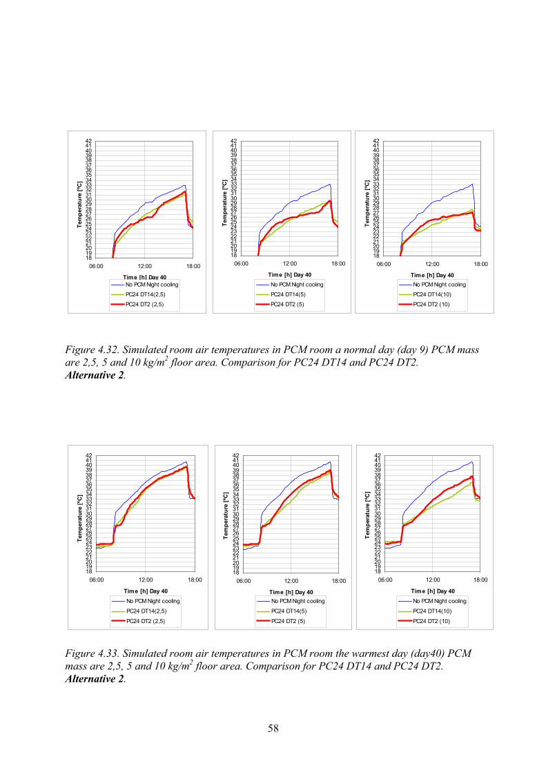
58

18192021222324252627282930313233343536373839404142

06:00 12:00 18:00

Time [h] Day 40

Tem

pera

ture

[ºC

]

No PCM Night cooling

PC24 DT14(10)

PC24 DT2 (10)

18192021222324252627282930313233343536373839404142

06:00 12:00 18:00

Time [h] Day 40

Tem

pera

ture

[ºC

]

No PCM Night cooling

PC24 DT14(5)

PC24 DT2 (5)

18192021222324252627282930313233343536373839404142

06:00 12:00 18:00

Time [h] Day 40

Tem

pera

ture

[ºC

]

No PCM Night cooling

PC24 DT14(2,5)

PC24 DT2 (2,5)

18192021222324252627282930313233343536373839404142

06:00 12:00 18:00

Time [h] Day 40

Tem

pera

ture

[ºC

]

No PCM Night cooling

PC24 DT14(5)

PC24 DT2 (5)

18192021222324252627282930313233343536373839404142

06:00 12:00 18:00

Time [h] Day 40

Tem

pera

ture

[ºC

]

No PCM Night cooling

PC24 DT14(2,5)

PC24 DT2 (2,5)

18192021222324252627282930313233343536373839404142

06:00 12:00 18:00

Time [h] Day 40

Tem

pera

ture

[ºC

]

No PCM Night cooling

PC24 DT14(10)

PC24 DT2 (10)

Figure 4.32. Simulated room air temperatures in PCM room a normal day (day 9) PCM mass are 2,5, 5 and 10 kg/m2 floor area. Comparison for PC24 DT14 and PC24 DT2. Alternative 2.

Figure 4.33. Simulated room air temperatures in PCM room the warmest day (day40) PCM mass are 2,5, 5 and 10 kg/m2 floor area. Comparison for PC24 DT14 and PC24 DT2. Alternative 2.

59

4.4.4 Cooling power

The cooling power of the heat exchanger is calculated as the mass flow times the temperature difference in the heat exchanger, see equation [3.18]. As the power is not a primary (measured) unit, the measured values can only be seen as an illustration. The cooling power is also simulated according to the scheme in Table 4.5. Examples of measured values for a normal day and the warmest day are shown in Figure 4.34, and cumulative distribution in Figure 4.35. In the example of day 9, the power output is near to constant, which means that the raise of temperature is equal in the PCM and in the room. For the warmest day (day 40) the temperature in the PCM becomes higher than the phase change temperature interval. This is seen as a sudden drop in the output. The power of the fan in the actual case is 72W. In the cumulative distribution curve this power crosses at 50% of the time. With a more careful selection of components and design a better result can be achieved.

Examples of simulated values for a normal day and the warmest day are shown in Figure 4.36 and Figure 4.37. Cumulative distribution is showed in Figure 4.38. As the power is not a measured primary unit, a comparison of measured and simulated curves of the day temperatures cannot be done. The very high power output in the simulations comes from the sudden changes in the changes from day to night case, so these values can be omitted in the diagrams. It shows in the simulated result that the mass of the PCM is the most deciding factor for the function of the system.

60

-180

-160

-140

-120

-100

-80

-60

-40

-20

-

06:00 09:00 12:00 15:00 18:00Time [h] Day 9

q [W

]-180

-160

-140

-120

-100

-80

-60

-40

-20

-

06:00 09:00 12:00 15:00 18:00Time [h] Day 40

q [W

]

Figure 4.34. Measured cooling power during a 56-day period from 2004-06-28. Day 9 and 40.

Figure 4.35. Cumulative frequency of measured cooling power measured from 08.00-20.00 during a 56-day period from 2004-06-28.

0102030405060708090

100

-200 -150 -100 -50 0

Cooling power [W]

%

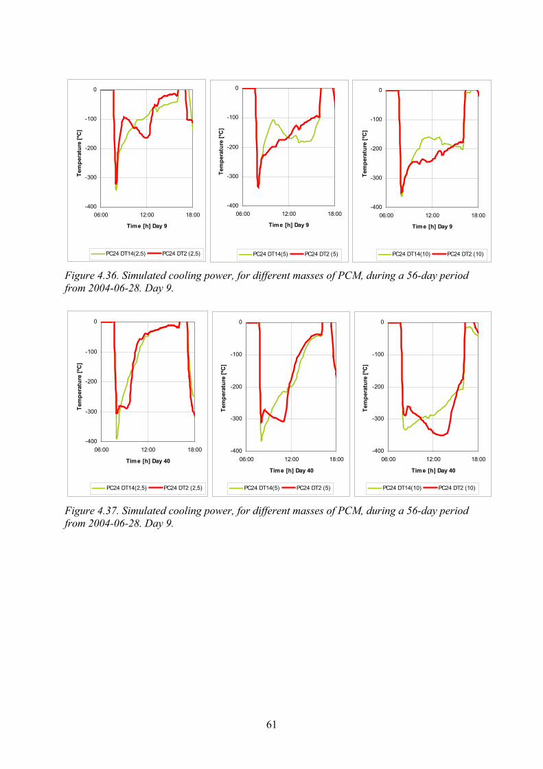
61

-400

-300

-200

-100

0

06:00 12:00 18:00

Time [h] Day 40

Tem

pera

ture

[ºC

]

PC24 DT14(5) PC24 DT2 (5)

-400

-300

-200

-100

0

06:00 12:00 18:00

Time [h] Day 40

Tem

pera

ture

[ºC

]

PC24 DT14(2,5) PC24 DT2 (2,5)

-400

-300

-200

-100

0

06:00 12:00 18:00

Time [h] Day 40

Tem

pera

ture

[ºC

]

PC24 DT14(10) PC24 DT2 (10)

Figure 4.36. Simulated cooling power, for different masses of PCM, during a 56-day period from 2004-06-28. Day 9.

Figure 4.37. Simulated cooling power, for different masses of PCM, during a 56-day period from 2004-06-28. Day 9.

-400

-300

-200

-100

0

06:00 12:00 18:00

Time [h] Day 9

Tem

pera

ture

[ºC

]

PC24 DT14(10) PC24 DT2 (10)

-400

-300

-200

-100

0

06:00 12:00 18:00

Time [h] Day 9Te

mpe

ratu

re [º

C]

PC24 DT14(5) PC24 DT2 (5)

-400

-300

-200

-100

0

06:00 12:00 18:00

Time [h] Day 9

Tem

pera

ture

[ºC

]

PC24 DT14(2,5) PC24 DT2 (2,5)

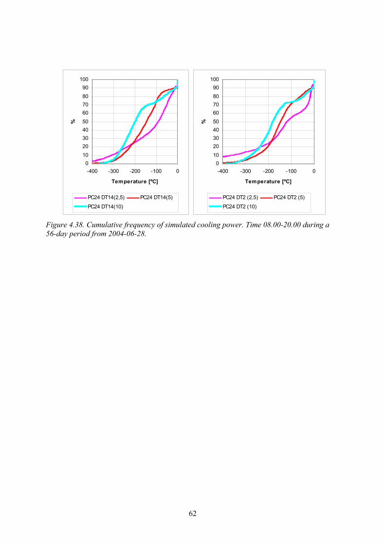
62

Figure 4.38. Cumulative frequency of simulated cooling power. Time 08.00-20.00 during a 56-day period from 2004-06-28.

0102030405060708090

100

-400 -300 -200 -100 0

Temperature [ºC]

%

PC24 DT14(2,5) PC24 DT14(5)

PC24 DT14(10)

0102030405060708090

100

-400 -300 -200 -100 0

Temperature [ºC]

%PC24 DT2 (2,5) PC24 DT2 (5)

PC24 DT2 (10)

63

5 DISCUSSION

5.1 General In this thesis, a night ventilation system, where the PCM is solidified with cool night air, and melted with warm indoor air during the day, is investigated. The stored thermal energy in the PCM is exchanged actively with fans. The aim of the application is to keep the indoor temperature to an acceptable level during summer time. The PCM that is used is a modified salt hydrate. As the material is expected to last for long time, it is essential to know if the performance of the material will change with time. There are known problems with salt hydrates in thermal cycling through its phase change, caused by incongruent melting. Another known problem is super cooling effect in the solidification of the material.

The application is investigated in three levels. First is an investigation of the performance of the thermal storage capacity when the PCM is cycled in different temperature intervals. This is done by water calorimeter measurements of large samples. The second level of the investigation is a development of a prototype air heat exchanger, where the PCM is used. Both experiments and theoretical model are made. The properties measured in the calorimeter are fed into the calculation model to verify the calculation method. The third level is the building of a semi full-scale test room where the prototype of the PCM air heat exchange is installed. Measurements of temperatures are done during the summer of 2004. During daytime the indoor air circulates in the PCM heat exchanger and the PCM melts. During nighttime the outdoor air is circulated in the heat exchanger and the PCM will solidify. This means that during a 24-hour cycle the PCM will go through one cycle of phase change. Measured properties are fed into the calculation model to verify the calculation method.

The main purpose of the work is to evaluate the performance over time for the PCM when the material will go through repeated cycles of phase changes in a temperature span close to room temperature. The estimation of the service life of the PCM will be based on the measured performance over time. The service life estimation is based on one or more critical properties of the material. In the theoretical models of the heat exchanger and the test room, different material properties can be assigned to the PCM. These different assignments of properties will mirror the results carried out in the calorimeter measurements.

The work with the prototype heat exchanger and the test room serves two purposes: development of the application, and evaluation of which property of the PCM that is critical in order to maintain the function of the application.

The service life estimations are based on the requirements 1, 2 and 3, that are presented in Table 1.2. These are general requirements valid for all PCM. In Table 1.3 the requirements of the European Building Product Directive are presented. In this project it is primarily requirement 6, energy economy and heat retention, that are considered.

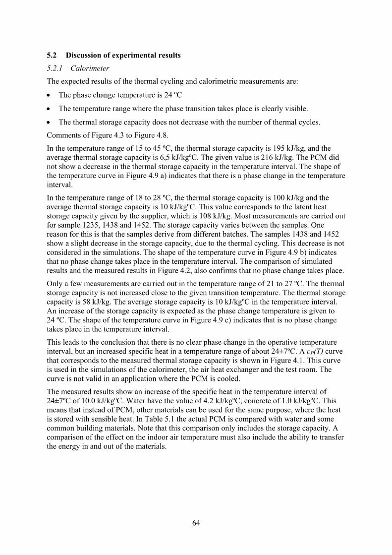
64

5.2 Discussion of experimental results

5.2.1 Calorimeter

The expected results of the thermal cycling and calorimetric measurements are:

• The phase change temperature is 24 ºC

• The temperature range where the phase transition takes place is clearly visible.

• The thermal storage capacity does not decrease with the number of thermal cycles.

Comments of Figure 4.3 to Figure 4.8.

In the temperature range of 15 to 45 ºC, the thermal storage capacity is 195 kJ/kg, and the average thermal storage capacity is 6,5 kJ/kgºC. The given value is 216 kJ/kg. The PCM did not show a decrease in the thermal storage capacity in the temperature interval. The shape of the temperature curve in Figure 4.9 a) indicates that there is a phase change in the temperature interval.

In the temperature range of 18 to 28 ºC, the thermal storage capacity is 100 kJ/kg and the average thermal storage capacity is 10 kJ/kgºC. This value corresponds to the latent heat storage capacity given by the supplier, which is 108 kJ/kg. Most measurements are carried out for sample 1235, 1438 and 1452. The storage capacity varies between the samples. One reason for this is that the samples derive from different batches. The samples 1438 and 1452 show a slight decrease in the storage capacity, due to the thermal cycling. This decrease is not considered in the simulations. The shape of the temperature curve in Figure 4.9 b) indicates that no phase change takes place in the temperature interval. The comparison of simulated results and the measured results in Figure 4.2, also confirms that no phase change takes place.

Only a few measurements are carried out in the temperature range of 21 to 27 ºC. The thermal storage capacity is not increased close to the given transition temperature. The thermal storage capacity is 58 kJ/kg. The average storage capacity is 10 kJ/kgºC in the temperature interval. An increase of the storage capacity is expected as the phase change temperature is given to 24 ºC. The shape of the temperature curve in Figure 4.9 c) indicates that is no phase change takes place in the temperature interval.

This leads to the conclusion that there is no clear phase change in the operative temperature interval, but an increased specific heat in a temperature range of about 24±7ºC. A cP(T) curve that corresponds to the measured thermal storage capacity is shown in Figure 4.1. This curve is used in the simulations of the calorimeter, the air heat exchanger and the test room. The curve is not valid in an application where the PCM is cooled.

The measured results show an increase of the specific heat in the temperature interval of 24±7ºC of 10.0 kJ/kgºC. Water have the value of 4.2 kJ/kgºC, concrete of 1.0 kJ/kgºC. This means that instead of PCM, other materials can be used for the same purpose, where the heat is stored with sensible heat. In Table 5.1 the actual PCM is compared with water and some common building materials. Note that this comparison only includes the storage capacity. A comparison of the effect on the indoor air temperature must also include the ability to transfer the energy in and out of the materials.

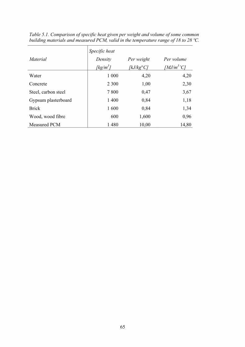
65

Table 5.1. Comparison of specific heat given per weight and volume of some common building materials and measured PCM, valid in the temperature range of 18 to 28 ºC.

Specific heat

Material Density Per weight Per volume

[kg/m3] [kJ/kg°C] [MJ/m3˚C]

Water 1 000 4,20 4,20

Concrete 2 300 1,00 2,30

Steel, carbon steel 7 800 0,47 3,67

Gypsum plasterboard 1 400 0,84 1,18

Brick 1 600 0,84 1,34

Wood, wood fibre 600 1,600 0,96

Measured PCM 1 480 10,00 14,80

66

5.2.2 Heat exchanger

In the application that is investigated in the project, the PCM is stored in a PCM heat exchanger unit. A simple calculation, Figure 4.10, shows that there are difficulties to load and unload the PCM storage in a room, unless the heat transfer between the indoor air and the PCM is enhanced. A prototype of the air heat exchanger is built and tested. Also, a mathematical model is made to explore the effect of different cP(T) curves. Measurements on the prototype are compared with simulated results and show agreement. This leads to the conclusion that simulations can be used to explore the effect on the heat exchanger for different cP(T) curves.

Simulations of the air heat exchanger, where the inlet temperature is constant, show that with a material that has a narrow melting temperature range, the cooling power output is close to constant throughout the phase transition. For materials that have a larger melting temperature range the cooling power is descending with time. The effect of this is that within a short time, the cooling power of the air heat exchanger will be lower than the power that is needed to run the fan.

The simulations of the air heat exchanger unit also show that the geometry of the heat exchanger is important for the function. The heat exchanger can be modelled as a fictive heat transfer coefficient, see equation [3.11]. The fictive heat transfer coefficient expresses the ability for the heat exchanger to store and release the stored energy. The airflow, the air velocity, the length and the heat transfer coefficient between the airflow and the PCM are the most governing factors. High airflows and short length give the highest fictive heat transfer coefficient. The heat transfer between the airflow and the PCM, can be enhanced with a rough surface. The air velocity should be so high that there is turbulent flow. But to high air velocity also gives a noise problem. The exchanger should be designed so the airflow through the unit is as high as possible in relation to the power input to the fan. The consequences of this are that the designer of the system must, in order to achieve a functional system, carefully design the unit in order to get the desired performance. The chosen components should use as little power as possible and should fit into the geometry. If this is not achieved, the unit will use more energy to run the system, than the delivered cooling energy.

The experiments and modelling of the air heat exchanger, also show that the cooling power output is linearly dependent on the temperature difference between the temperature that enters the heat exchanger and the temperature in the PCM. This implies that the phase change temperature, or the transition temperature, is important for the function of the system. PCM with a narrow temperature range is the most desirable material.

The mass of PCM and the way in which the PCM is stored, are also important for the function of the application. This is an important factor for the economic evaluation of the application. The heat transfer coefficient of the system is dependent on the heat resistance in the material. The thickness of the storage therefore must be optimised in order to achieve the desired effect. A simplified conclusion of this is that the power is dependent on the airflow and contact area, and the energy that is released and stored is dependent on the mass of the PCM storage.

The critical properties of the PCM concerning the function of the heat exchanger, are the thermal storage capacity, the melting temperature and the melting temperature range. The critical property of the equipment is its power and energy efficiency.

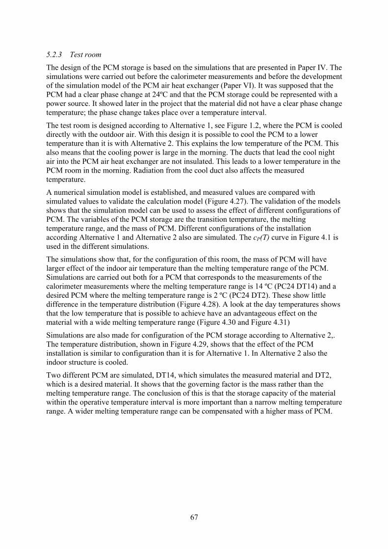
67

5.2.3 Test room

The design of the PCM storage is based on the simulations that are presented in Paper IV. The simulations were carried out before the calorimeter measurements and before the development of the simulation model of the PCM air heat exchanger (Paper VI). It was supposed that the PCM had a clear phase change at 24ºC and that the PCM storage could be represented with a power source. It showed later in the project that the material did not have a clear phase change temperature; the phase change takes place over a temperature interval.

The test room is designed according to Alternative 1, see Figure 1.2, where the PCM is cooled directly with the outdoor air. With this design it is possible to cool the PCM to a lower temperature than it is with Alternative 2. This explains the low temperature of the PCM. This also means that the cooling power is large in the morning. The ducts that lead the cool night air into the PCM air heat exchanger are not insulated. This leads to a lower temperature in the PCM room in the morning. Radiation from the cool duct also affects the measured temperature.

A numerical simulation model is established, and measured values are compared with simulated values to validate the calculation model (Figure 4.27). The validation of the models shows that the simulation model can be used to assess the effect of different configurations of PCM. The variables of the PCM storage are the transition temperature, the melting temperature range, and the mass of PCM. Different configurations of the installation according Alternative 1 and Alternative 2 also are simulated. The cP(T) curve in Figure 4.1 is used in the different simulations.

The simulations show that, for the configuration of this room, the mass of PCM will have larger effect of the indoor air temperature than the melting temperature range of the PCM. Simulations are carried out both for a PCM that corresponds to the measurements of the calorimeter measurements where the melting temperature range is 14 ºC (PC24 DT14) and a desired PCM where the melting temperature range is 2 ºC (PC24 DT2). These show little difference in the temperature distribution (Figure 4.28). A look at the day temperatures shows that the low temperature that is possible to achieve have an advantageous effect on the material with a wide melting temperature range (Figure 4.30 and Figure 4.31)

Simulations are also made for configuration of the PCM storage according to Alternative 2,. The temperature distribution, shown in Figure 4.29, shows that the effect of the PCM installation is similar to configuration than it is for Alternative 1. In Alternative 2 also the indoor structure is cooled.

Two different PCM are simulated, DT14, which simulates the measured material and DT2, which is a desired material. It shows that the governing factor is the mass rather than the melting temperature range. The conclusion of this is that the storage capacity of the material within the operative temperature interval is more important than a narrow melting temperature range. A wider melting temperature range can be compensated with a higher mass of PCM.

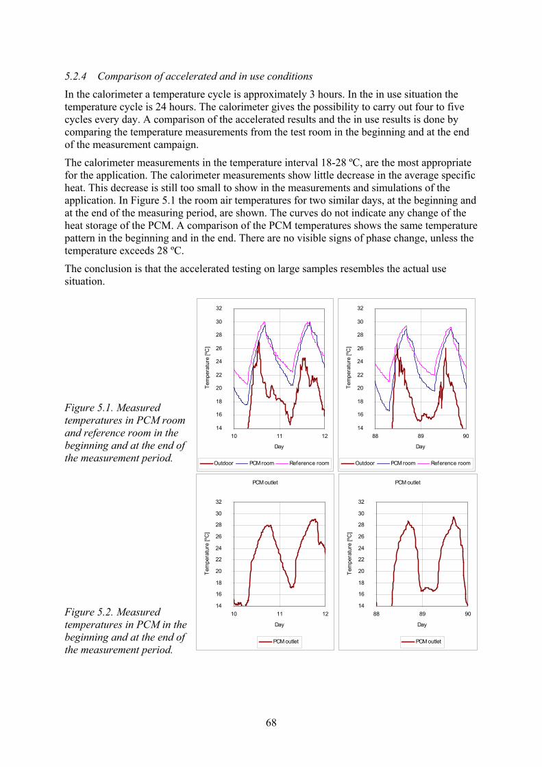
68

PCM outlet

14

16

18

20

22

24

26

28

30

32

10 11 12

Day

Tem

pera

ture

[ºC

]

PCM outlet

PCM outlet

14

16

18

20

22

24

26

28

30

32

88 89 90

Day

Tem

pera

ture

[ºC

]

PCM outlet

14

16

18

20

22

24

26

28

30

32

10 11 12

Day

Tem

pera

ture

[ºC

]

Outdoor PCM room Reference room

14

16

18

20

22

24

26

28

30

32

88 89 90

Day

Tem

pera

ture

[ºC

]

Outdoor PCM room Reference room

5.2.4 Comparison of accelerated and in use conditions

In the calorimeter a temperature cycle is approximately 3 hours. In the in use situation the temperature cycle is 24 hours. The calorimeter gives the possibility to carry out four to five cycles every day. A comparison of the accelerated results and the in use results is done by comparing the temperature measurements from the test room in the beginning and at the end of the measurement campaign.

The calorimeter measurements in the temperature interval 18-28 ºC, are the most appropriate for the application. The calorimeter measurements show little decrease in the average specific heat. This decrease is still too small to show in the measurements and simulations of the application. In Figure 5.1 the room air temperatures for two similar days, at the beginning and at the end of the measuring period, are shown. The curves do not indicate any change of the heat storage of the PCM. A comparison of the PCM temperatures shows the same temperature pattern in the beginning and in the end. There are no visible signs of phase change, unless the temperature exceeds 28 ºC.

The conclusion is that the accelerated testing on large samples resembles the actual use situation.

Figure 5.1. Measured temperatures in PCM room and reference room in the beginning and at the end of the measurement period.

Figure 5.2. Measured temperatures in PCM in the beginning and at the end of the measurement period.

69

5.2.5 Energy efficiency of the system

The estimations of unloading time shown in Figure 4.10, show that it could be difficulties to unload a storage of PCM with air, with natural convection. Therefore it is necessary to force the convection to exchange the stored energy. The time it takes to load and unload the PCM storage is dependent on the fictive heat transfer coefficient αP and the temperature difference. This leads to a problem, the cooling power must be greater than the power of the fan that runs the system. If the design of the heat exchanger and the fan system is not designed carefully, one will end up only with a fan that moves the indoor air around and heats the room. One of the aims with the system is that both the power and the energy consumption should be low. This obvious requirement implies that the design of the system is crucial for the energy-related performance of the system.

In order to get an efficient system the following components must be optimised: The geometry of the heat exchanger must be optimised, according to the desired loading and unloading time. Looking into the expression of the fictive heat transfer coefficient, one can see that a high airflow and a short length are the most deciding factors to achieve high heat transfer. The air velocity and the properties surface must also be formed to get a turbulent flow. But there are practice limitations in the velocity. If the air velocity is too high there will be a noise problem, and if the air gap is too small, there is also a problem of pressure drop in the system. In the design of the heat exchanger, it might be obvious, at first thought, to make a long exchanger, in order to achieve as large temperature difference as possible. But too long a distance, for the air, will lead to two problems. The fictive heat transfer coefficient is lower and the pressure drop increases.

It is necessary to design a system with as low pressure drop as possible and choose a fan that is efficient for this particular use. In the design of the test room these problems are not fully considered. The airflow in the daytime loop is approximately 0.07 m3/h and the fan power is 72 W. The ratio between the airflow and the power use could have been improved, for example by using a DC motor and a larger diameter of the propeller of the fan.

The control of the run-times of the fans and airflows are also important in order to get an efficient system. The parameters that can be measured are the air temperatures and the PCM temperatures. The test room does not have any regulation of airflow according to the measured temperatures. An optimisation of the design would increase the system efficiency.

In Figure 1.2, two different configurations of the system are shown. The choice of which alternative is the most efficient must be decided for each case. The advantage with Alternative 1 is that it is possible to cool the PCM to a lower temperature. With a system solution according to Alternative 2, it is possible to involve the rest of the structure in the night cooling.

The type of system that is presented in this thesis works much in the same way as if the building would have a high thermal inertia. Therefore there must be a temperature rise in the building in order to unload the stored energy in the PCM. The system cannot be compared to air conditioning system. Possibly, the energy efficiency of the systems can be compared. An increase of the overall efficiency of the system would be obtained if the PCM storage also was used during the warming season of the building. The PCM should in this case be used to store energy when the indoor temperatures rise above an acceptable level during the afternoon, and release the energy in the following morning.

70

5.3 Service life of PCM The service life of a product is based on the performance of one or more critical properties, the performance requirements and the degradation environment, Figure 5.3.

Figure 5.3. Schematic picture of service life estimation

5.3.1 Performance requirements

The performance requirements of the application are discussed in 1.5.2 and can be concluded in:

• The phase transition process must be completely reversible and only temperature dependent.

• The phase transition temperature must match the practical temperature range of the application.

• The material must have a large latent heat and high thermal conductivity. The material is chemical stable such that no chemical composition occurs.

The use in building application sets special requirements to the materials. According to the European Construction Directive (CPD 1988), six essential requirements must be fulfilled for materials. The requirement that is investigated in this project is:

• Energy economy and heat retention

Performance

Time Service life

Performance requirement

Performance of critical property as function of degradation environment

71

5.3.2 Critical properties of application

The service life of the PCM and the application that it is used in, will be based on the critical properties of the system. According to the discussion above, the critical properties of the PCM in its application are the thermal storage capacity, the phase change temperature and the melting temperature range. The measurement of thermal properties shows that the operative temperature interval is a critical property. According to the energy efficiency of the application, the energy use to exchange the stored energy is the critical property.

5.3.3 Degradation environment

The degradation environment in the actual application is the temperature cycling in the operative temperature interval.

5.3.4 Service life discussion

In my licentiate thesis it is proposed that the service life of a product can be assessed in three different ways. At first, there is the “dose response approach”, where gradual degradation of components takes place due to a specific dose of a degradation agent. The second approach is to draw conclusions of the service life from observed maintenance intervals in the built environment. Thirdly, is the “risk assessment approach”. It is adopted for such components that are not subjected to continuous degradation but had an instant failure, due to special conditions. What method should be used to assess the service life of PCM components? It is clear that the service life of a phase change material should be based on a dose response function or a damage function. The accelerated testing of the material agrees with the results obtained in the condition use of the material. The dose or the degradation agent of the PCM is the temperature cycling of the material.

The calorimeter measurements and the temperature measurements in the test room showed that there is no clear phase change in the operative temperature interval. But there is an increased specific heat in the actual interval, compared to the specific heat in liquid and solid phase. This fact is tested in simulation of the heat exchanger and the room simulation. It shows to have a clear negative influence of the cooling power output of the heat exchanger when the input air temperature is constant. The effect is not as clear in the simulation of the room. The property that is most important in the room application is the storage capacity in the whole operative temperature interval. The performance is better with a low melting temperature range but is not crucial for the performance of the application. The wide melting temperature range can be compensated with an increase of the PCM mass.

The calorimeter measurements of the PCM show a decrease in the thermal storage capacity in the measurement in the temperature range of 18-28 ºC. In the temperature ranges of 15-45 ºC and of 21-27 ºC, this tendency did not show. However, it is clear that a function of the long time behaviour can be established if a tendency of decrease of the thermal storage capacity should show in the measurements.

According to Table 1.1 the design lives of services components range from 10 to 25 years. Is the service life of this PCM in this range? If the PCM is stored in a steady temperature, i.e. it is not thermally cycled, it will recover to its former thermal storage capacity. In Paper VII it is shown for one of the samples. One sample is stored in room temperature for six months. When the sample is measured in the calorimeter, the thermal storage capacity is higher in the first cycles to approach the former measured value in a few cycles. This indicates that the service life of the PCM in this particular application is within the range of the DLC of the services.

72

73

6 CONCLUSIONS In the project presented in this thesis, development of a PCM based night cooling system is carried out. Along with this development, the service life of the PCM and its use in the application is estimated. In the application cool night air is used to cool the indoor air during daytime. The PCM is a modified hydrated salt. Storing the PCM in an air heat exchanger unit enhances the heat transfer from the indoor air to the PCM. The intended use for the application is in lightweight buildings with a low thermal inertia where there is an over production of heat like schools, offices and shopping centres. The effect in heavyweight buildings is limited.

A program is set up in order to develop and perform performance over time testing PCM. The testing procedure is set up according to ISO standards. The tests are focused on the change over time of the heat storage capacity in the operative temperature interval 18 to 28 ºC. Measurements are carried out with water bath calorimeter designed for this particular purpose.

Parallel to the calorimeter measurements, development of the application is carried out. A prototype of the heat exchanger is placed in a test room. Attached to the test room is a reference room and the temperatures in the rooms are measured and compared. The effect of the night cooling system is similar to an increase of the thermal inertia, but the storage and release of energy is controlled with fans. This leads to the fact that the cooling effect of the application is dependent mostly on the mass of the installed PCM and on the ability to exchange the energy in an efficient way. A theoretical model of the heat exchanger and the test room is made and a simulation model is created. Results from the calorimeter measurements are fed into simulation models in order to evaluate the results. Proposals of enhancements are presented and different configurations of the night cooling system are evaluated.

Service life estimations components and material are based on the performance over time of one or more critical properties. If the performances of these properties are below the performance requirements after a period time, the material reaches its service life. The critical properties of the PCM are evaluated in the experiments and in the simulations of the application. The performance requirements of the material are set up according to general requirements of PCM and requirements according to the European Construction Product Directive (CPD 1988).

The critical properties of a PCM are the transition temperature, the melting temperature range and the storage capacity in the operative temperature interval. The critical property of the application is its energy efficiency. The result of the investigation can be concluded in:

• The night cooling system will lower the indoor day temperatures; this works as if the thermal inertia is increased in lightweight buildings. The mass of PCM and the design of the system are critical to the system efficiency.

• The thermal storage capacity is increased in the operative temperature interval, but the effect of a clear phase change does not show. In the application this can be compensated with an increase of the mass of PCM.

• The service life of the PCM is expected to be within the range of design lives of services components.

74

75

7 FUTURE WORK The research project that is presented in this thesis follows two lines: performance over time testing of PCM and development of a night cooling application. Both these lines need to be followed up in future works.

The results of the development of the application can be used directly to design night cooling systems. To get more efficient systems, work needs to be carried out in the design of the PCM storage, choice of fans and configuration of the system. Also integration of the findings can be implemented in software for simulation of different climatic conditions. As the system will work in any climatic context where there is a temperature swing from night to day, an investigation in different climates in the world, including desert climate, should be carried out.

The possibility to design an efficient system is dependent on the accuracy of the presented thermal material properties of the PCM. Therefore it is desirable that standardized testing methods are established, and standardized classification systems of PCMs are developed.

The method of direct measuring of the storage capacity on samples, which resembles the shape in the actual application, is a promising technique. The calorimetric equipment presented in the thesis needs development for a better and more reliable function. It works in the melting phase. Equipment is needed also to measure the energy exchange in the solidification phase.

76

77

8 REFERENCES ABHAT A., 1983. Low temperature latent heat temperature storage: Heat storage materials.

Solar Energy, Vol. 30, No. 4, pp. 313-332.

ATHIENITIS, A.K.; LIU, C.; HAWES, D.; BANU, D.; FELDMAN, D., 1997. Investigation of the thermal performance of a passive solar test. Building and Evironment, Vol. 32, No 5, pp. 405-410.

BANARD, N., (2002). Thermal Mass and Night Ventilation – Utilising “Hidden” Thermal Mass. The International Journal of Ventilation, Volume 1: Issue 2, October 2002.

BARTON P.; BEGGS C.B.; SLEIGH P.A., 2002. A theoretical study of the thermal performance of the TermoDeck hollow core slab system. Applied Thermal Engineering, September 2002, vol. 22, no. 13, pp. 1485-1499(15) Elsevier Science

BELLANDER R., HED G., 2005. Water calorimetric measurements of large samples of phase change material (Paper to be published)

BONACINA C., COMINI G., FASANO A., PRIMICERIO M., 1973. Numerical solution of phase change problems, International Journal of Heat and Mass Transfer, 16, (1973), 1825-1832.

BROWN P. W., GRIMES II J., W.; KAETZEL, L., 1986. Evaluation of the variation in thermal performance in a NA2SO4 10H2O phase change system. Solar Energy Materials, v 13, n 6, Jul, 1986, p 453-461

BYUNG C. S., SANG D. K.; PARK, W.H., 1989. Phase separation and supercooling of a latent heat-storage material. Energy (Oxford). Volume 14, n 12, Dec, 1989, p 921-930

CARLSSON B., STYMNE H., WETTERMARK G., 1978. Storage of low-temperature heat in salt-hydrate melts – calcium chloride hexahydrate. Swedish Council for Building Research. Document D12:1978. ISBN 91-540-2889-2.

CPD (1988), COUNCIL DIRECTIVE of 21 December 1988 on the approximation of laws, regulations and administrative provisions of the Member States relating to construction products. (EG:s direktiv rörande byggprodukter) ISBN 91-85548-38-3.

CROWE, C. T., ELGER D., ROBERTSON J. A., 2001. Engineering Fluid Mechanics 7th edition, John Wiley & Sons, Inc. ISBN 0-471-38482-8.

FARID, M. M., KHUDHAIR, A.M.; RAZACK, S. A. K.; AL-HALLAJ, S., 2003. A review on phase change energy storage: Materials and applications. Energy Conversion and Management, v 45, n 9-10, June, 2004, p 1597-1615

FEUSTEL H. E. AND STETIU C., 1997. Thermal Performance of Phase Change Wallboard for Residential Cooling Application Indoor. Environment Program Energy and Environment Division Lawrence Berkeley National Laboratory University of California Berkeley, CA 94720, USA. April 1997. http://epb1.lbl.gov/thermal/pcm1.pdf

78

HASNAIN, S.M.,1998. Review on sustainable thermal energy storage technologies, Part I: Heat storage materials and techniques (King Abdulaziz City for Science and Technology) Source: Energy Conversion and Management, v 39, n 11, Aug, 1998, p 1127-1138

HE, B., 2004: High-Capacity Cool Thermal Energy Storage for Peak Shaving. Thesis (PHd),. TRITA-KET R195. ISSN 1104-3466. ISBN 91-7283-751-9. Royal University of Technology, Stockholm, Sweden 2004

HED G., 2000. Service life planning in building design. Thesis (Lic.). Centre of Built Environment, University of Gävle. Research School on Built Environment. RD-report No 4.

HED G., BELLANDER R. 2005. Mathematical modelling of PCM air heat exchanger Energy and buildings

HED G., BELLANDER R., 2005. Service life testing of PCM based components in buildings. Proceedings of: 10DBMC International Conférence On Durability of Building Materials and Components, LYON [France] 17-20 April 2005

HED G., 1999. Service life planning carried out in a building project The International Journal of Low Energy and Sustainable Buildings. http://www.byv.kth.se/avd/byte/leas/

HETENY, J., LAGERKVIST K.O., 1981. Långtidstest genom cycling av ett saltsmältlager med glaubersalt som energilagringsmaterial. (Long-term testing by cycling a phase-change heat store with glauber salts as an energy storage material). Teknisk rapport SP-RAPP 1981:05. Borås, Sweden 1981.

HOLMAN J. P. 1997. Heat Transfer, 8th edition. McGraw Hill, Inc. ISBN 0-07-844785-2

ISO 15686-1, 2000, Buildings and constructed assets – Service life planning, part 1, General principles. International Organization for Standardization.

ISO 15686-2, 2001. Buildings and constructed assets – Service life planning, part 2, Service life prediction principles. International Organization for Standardization

JOHANNESSON G., 2002. Lectures on building physics, Heat and moisture transfer. Kungliga Tekniska Högskolan, Stockholm 2002.

JOHANSSON U., 2001. DCN analysis of PCM. SP Report F1 16387

LAMBERG P., LEHTINIEMI R. AND HENELL A.-M. 2003. Numerical and experimental investigation of melting and freezing processes in phase change material storage. International Journal of Thermal Sciences, in press. © 2003 by authors and © 2003 Elsevier Science.

79

LAMBERG P., JOKISALO J., SIRÉN K., 2000. The effects on indoor comfort when using phase change materials with building concrete products. In proceedings of: IEA Annex 10 “Phase change materials and chemical reactions for thermal energy storage”. Sixth Workshop, Stockholm, Sweden, 22-24 November 2000. http://www.fskab.com/ANNEX10/WS_pres/Lamberg.pdf

MARÍN, J.M.; ZALBA, B.; CABEZA, L.F.; MEHLING, H., 2003. Determination of enthalpy-temperature curves of phase change materials with the T-history method - improvement to temperature dependent properties. Measurement Science and Technology, 14, 184-189, 2003.

MARTEINSSON, B., 2003. Assessment of Service Lives in Design of Buildings – Development of the Factor Method. Thesis (Lic.). KTH´s Research School, Centre of Built Environment, University of Gävle. BMG-MT TR01-2003. ISBN 91-7283-586-9.

MARTIN V., RYDSTRAND M AND HE B., 2003. On the effective design of a PCM cool storage in comfort cooling applications – the importance of narrow phase change temperature ranges. In the proceedings of: IEA Annex 17 Workshop EM3 Tokyo 2002. http://www.fskab.com/Annex17/

MATHSOFT, Mathcad 11, User´s guide, 2002.

MEHLING H, S. HIEBLER S, . CABEZA L. F., 2002. News on the application of PCM:s for heating and cooling of buildings. In proceedings of: IEA Annex 17, Phase change materials and chemical reactions for thermal energy storage. Tokyo 2002-09-30--10-02. http://www.fskab.com/Annex17/index.htm

NEEPER, D.A. 2000. Thermal dynamics of wallboard with latent heat storage (Science & Engineering Associates, Inc) Source: Solar Energy, v 68, n 5, 2000, p 393-403

LAMBERG P., JOKISALO J. , SIRÉN K., 2000. The effects on indoor comfort when using phase change materials with building concrete products. In proceedings of: IEA Annex 10 “Phase change materials and chemical reactions for thermal energy storage. Sixth Workshop, Stockholm, Sweden, 22-24 November 2000. http://www.fskab.com/ANNEX10/WS6.htm

PILLAI, K. K.; BRINKWORTH, B. J., 1976. Storage of low grade thermal energy using phase change materials. Applied Energy, v 2, n 3, Jul, 1976, p 205-216

ROUCOULT, J.-M. Douzane, O.; Langlet, T., 1999. Incorporation of thermal inertia in the aim of installing a natural nighttime ventilation system in buildings; Energy and Buildings, v 29, n 2, Jan, 1999, p 129-133

RYU H. W., WOO S. W.; SHIN, B. C.; KIM, S. D., 1992. Prevention of supercooling and stabilization of inorganic salt hydrates as latent heat storage materials, Solar Energy Materials and Solar Cells. Volume 27, n 2, Jul, 1992, p 161-172

80

SCALAT, S., BANU, D.; HAWES, D.; PARIS, J.; HAGHIGHATA, F.; FELDMAN, D. 1996. Full scale thermal testing of latent heat storage in wallboard. Solar Energy Materials and Solar Cells, v 44, n 1, Oct 30, 1996, p 49-61

STETIU C. FEUSTEL H. E. Phase Change Wallboard and Mechanical Night Ventilation in Commercial Buildings Lawrence Berkeley National Laboratory, Berkeley, CA http://epb1.lbl.gov/thermal/pcm2.pdf

STOCKERL, R., KOHLER, H.-H., 1991. Dynamic investigations of the slow recrystallization of incongruently melting Glauber salt. Solar Energy, v 46, n 3, 1991, p 167-173

WINWOOD R., BENSTEAD R.; EDWARDS R., 1997. Advanced fabric energy storage I: review (EA Technology); Building Services Engineering Research & Technology, v 18, n 1, 1997, p 1-6

YAMAHA, M., 1999. A simulation model for thermal response of PCM installed in air distribution system. In proceedings of IEA Annex 10 “Phase change materials and chemical reactions for thermal energy storage”. Third Workshop, 27-28 May 1999, Helsinki, Finland. http://www.fskab.com/ANNEX10/workshops.htm

ZALBA B., MARIN J. MA, CABEZA L. F., MEHLING H., 2003. Review on thermal storage with phase change materials, heat transfer analysis and applications. Applied Thermal Engineering 23 (2003) 251-283