UNIVERSIDAD NACIONAL DE CÓRDOBA

FACULTAD DE MATEMÁTICA, ASTRONOMÍA Y FÍSICA ______________________________________________________________________

SERIE “A”

TRABAJOS DE MATEMÁTICA

Nº 110/2011

A PARAMETER ESTIMATION PROBLEM FOR A TUMOUR GROWTH MODEL

D.A. Knopoff, D.R. Fernández, G.A. Torres, C.V. Turner

Editores: Jorge G. Adrover – Gastón García CIUDAD UNIVERSITARIA – 5000 CÓRDOBA

REPÚBLICA ARGENTINA

A parameter estimation problem for a tumour growth model .

D. A. Knopoff, D. R. Fernandez, G. A. Torres and C. V. Turner∗

FaMAF, Universidad Nacional de Cordoba - CIEM-CONICET. Cordoba, Argentina.

Abstract

In this paper we present a method for estimating unknown parameters that appear on anavascular, spheric tumour growth model. The model for the tumour is based on nutrient drivengrowth of a continuum of live cells, whose birth and death generate volume changes describedby a velocity field. The drug is applied externally, and is assumed to be a diffusible substancecapable of killing cells.

The model consists on a coupled system of partial differential equations which is solvednumerically. As the domain on which the equations are definedis the tumour, that changes in sizeover time, the problem can be formulated as a moving boundaryone.

After solving the forward problem properly, we are concerned in using the model for theestimation of parameters, by fitting the numerical solutionwith real data. We define a functionalto compare both of them and we use the pattern search method for minimizing it, obtaining goodaccuracy for the recovery of a few parameters.

Keywords: avascular tumour, constrained optimization, inverse problem, mathematical modeling.

1 Introduction.

The interest for research in modeling cancer has grown enormously over the last decades, [1, 2].Pioneers have been, for example, [11, 15], where the first spatio-temporal models of an avascularmulticellular spheroid’s (MCS) growth have been developed. The study of MCS is interesting be-cause they provide the best insight into the effectiveness of chemotherapeutic drugs on tumours invivo, and their behaviour can be studied experimentally (invitro) by controlling environmental con-ditions in which they grow: for example, the radii of the tumour can be monitored by changing thechemotherapeutic drug or oxygen levels.

In addition, another variables can be measured. If possible, experimentalists can get informationabout the distribution of substances within the tumour. Moreover, via medical imaging or histologicalcuts, they can also get data about the density of the different kind of cells conforming it: proliferating,quiescent, necrotic.

That is why in this general approach of modeling the key variables are the tumour size (radius)and the concentration within the tumour of growth-rate limiting diffusible chemicals (nutrients suchas oxygen or glucose or a chemotherapeutic drug). Since the tumour changes in size over time, thedomain on which the models are formulated must be determinedas part of the solution process, givinga vast class of moving boundary problems, [6, 7].

In this article, we propose a framework for estimating unknown parameters via PDE-constrainedoptimization, following the PDE-based model by Ward and King, [16]. In this approach, avascular

∗E-mail address: knopoff@famaf.unc.edu.ar, dfernandez@famaf.unc.edu.ar, torres@gmail.com,turner@famaf.unc.edu.ar

1

tumour growth is modeled via a coupled nonlinear system of differential equations, which make thenumerical solution procedure quite challenging.

We are concerned with developing a robust PDE-constrained formulation that let us find the bestset of parameters of a tumour growth model that fits patient orexperimental data. We choose theparameters that should be of applied interest and try to obtain them by defining a functional to beminimized.

The paper is organized as follows: section 2 introduces the tumour growth model (forward prob-lem). Section 3 shows the numerical solution of the forward problem and checks its accuracy byproving some theoretical results. Section 4 introduces theinverse problem approach, by defining thefunctional to be minimized. Finally, in section 5 the numerical procedure to solve the inverse problemis discussed.

2 Mathematical model.

We consider the model proposed by Ward and King in [16]. The tumour is a spheroid which consistsof a continuum of living cells, in one of two states: live or dead. The rates of birth and death dependon the nutrient and chemotherapeutic drug concentration. It is supposed that those processes generatevolume changes, leading to cell movement described by a velocity field. The system of equations tobe studied is:

∂n∂t

+1r2

∂(r2vn)∂r

= [km(c)−kd(c)−KG(km(c))w]n, (2.1)

∂c∂t

+1r2

∂(r2vc)∂r

=Dr2

∂∂r

(r2 ∂c

∂r

)−βkm(c)n, (2.2)

1r2

∂(r2v)∂r

= [VLkm(c)− (VL −VD){kd(c)+KG(km(c))w}]n, (2.3)

∂w∂t

+1r2

∂(r2vw)∂r

=Dw

r2

∂∂r

(r2 ∂w

∂r

)−

Kω

G(km(c))wn, (2.4)

where the dependent variablesn, c, v and w are the live cell density (cells/unit volume), nutrientconcentration, velocity and drug concentration, respectively. As it is described in [16], equation (2.1)states that the rate of change ofn is dependent on the difference between the birthkm(c) and deathkd(c) rates, where this one is either natural (as described in [17]) or due to the drug effects, at a rateKG(km(c))w. The functonskm andkd are taken to be generalised Michaelis-Menten kinetics withexponent 1, i.e.

km(c) = A

(c

cc+c

), (2.5)

kd(c) = B

(1−σ

ccd +c

). (2.6)

The constantK is the maximum possible rate of drug induced cell death. The constantsA, B andσare positive parameters of the Michaelis-Menten kinetics,while cc andcd are critical concentrations.G(km(c)) is a function that represents the dependence between drug action and cell-cycle. As it isconsidered in [16] it is a good idea to choose a linear dependence, giving

G(km(c)) = km(c)/A.

2

Equation (2.2) states that the nutrient is consumed at a rateproportional to the rate of mitosis,and its diffusion is described by Ficks law. Equation (2.3) states that the rate of volume change isgiven by the difference in volume generated via birth from that lost by death (it is assumed that a livecell occupies a volumeVL that is twice the volume of a death cellVD). The diffusion of the drug isdescribed also by Ficks law, and it is assumed that it is degraded only when it attacks a living cell,giving a maximum degradation rateK/ω. ω is a dimensionless constant that can be interpreted as ameasure of the drugs effectiveness, as explained in [16], with increasingω implying that less drugis consumed to produce the same effects during the killing process. These considerations lead toequation (2.4).

2.1 Moving boundary problem

As it has been mentioned, the tumour is assumed to be a spheroid that exhibits radial simmetry. Thatis why, not only the state variablesn, c, v andw are important, but the outer tumour radius is also akey variable to be determined. Since the tumour changes in size over time, the domains on which themodels are formulated (and the PDEs are valid) must be determined as part of the solution.

Let S(t) be the tumour radius at timet. So, if we suppose that the treatment begins at timet = 0,in which the tumour has a radiusSI , with living cell density and nutrient concentration distributionsnI (r) andcI (r), respectively, then the initial conditions of the problem can be formulated as

n(r,0) = nI (r), (2.7)

c(r,0) = cI (r), (2.8)

w(r,0) = 0, (2.9)

S(0) = SI . (2.10)

Because symmetry is assumed about the tumour center, there is no flux there. That is why, asboundary conditions aboutr = 0, are taken:

∂c∂r

(0, t) = 0, (2.11)

v(0, t) = 0, (2.12)∂w∂r

(0, t) = 0. (2.13)

Moreover, on the external boundary (which is also the boundary of the complement of the tumouras a subset of the body), the following conditions are taken:

c(S(t), t) = c0, (2.14)dSdt

= v(S(t), t), (2.15)

w(S(t), t) = w0(t), (2.16)

wherec0 andw0(t) are external nutrient and drug concentrations, respectively. The functionw0(t)depends on the chemotherapeutic protocol. In our simulations it will be considered as a constant thatdoes not depend ont. However, other functions may be adopted, for example in section 3 we showan example in which drug is provided for some intervals of time, but not for other ones.

3

2.2 Nondimensionalisation

Before analysing the model equations, we re-scale the mathematical model in the following way,denoting non-dimensional variables with bars:

n=VLn; c= c/c0; v= v/r0A; t = At r = r/r0; S= S/r0; w= w/W0

wherer0 = (3VL/4π)1/3 is the radius of a single cell andW0 is a suitable reference drug concentration(typically W0 = max(w0(t))).

It is important to remark that inherent in this problem are two timescales: the tumour growthtimescale (≈ 1 day) and the much shorter drug and nutrient diffusions (≈ 1 min). That is why,following [2, 1, 16, 6] we adopt a quasi-steady assumption inthe nutrient and drug equations.

Following [16], and relabeling the variables with bar againwithout it, these rescalings lead to thefollowing system of differential equations:

∂n∂t

+v∂n∂r

= [a(c,w)−b(c,w)n]n, (2.17)

1r2

∂∂r

(r2 ∂c

∂r

)= k(c)n, (2.18)

1r2

∂(r2v)∂r

= b(c,w)n, (2.19)

1r2

∂∂r

(r2∂w

∂r

)=

Kα

km(c)wn, (2.20)

where

α = ωDwVLW0/Ar20, (2.21)

K = KW0/A,

a(c,w) =1A[km(c)−kd(c)−KG(km(c))w],

b(c,w) =1A{km(c)− (1−δ)[kd(c)−KG(km(c))w]},

k(c) = βkm(c)/A,

with δ =VD/VL and(β) = r20βA/VLc0D.

We note that theconstantα defined above comprises many model parameters that should beinteresting to know exactly. It will be of great importance in the next sections, whereα will beconsidered as a key parameter of the problem.

Also, it is worth saying that rigorous mathematical analysis including existence, uniqueness, andstability theorems, as well as properties of the free boundaries for similar tumour growth models inwhich different kind of PDEs are combined, have been obtained, [4] and [8].

4

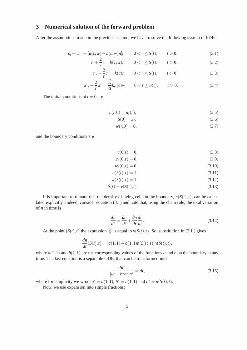
3 Numerical solution of the forward problem

After the assumptions made in the previous section, we have to solve the following system of PDEs:

nt +vnr = [a(c,w)−b(c,w)n]n 0< r ≤ S(t), t > 0, (3.1)

vr +2r

v= b(c,w)n 0< r ≤ S(t), t > 0, (3.2)

crr +2r

cr = k(c)n 0< r ≤ S(t), t > 0, (3.3)

wrr +2r

wr =Kα

km(c)w 0< r ≤ S(t), t > 0. (3.4)

The initial conditions att = 0 are

n(r,0) = nI (r), (3.5)

S(0) = SI , (3.6)

w(r,0) = 0, (3.7)

and the boundary conditions are

v(0, t) = 0, (3.8)

cr(0, t) = 0, (3.9)

wr(0, t) = 0, (3.10)

c(S(t), t) = 1, (3.11)

w(S(t), t) = 1, (3.12)

S(t) = v(S(t), t). (3.13)

It is important to remark that the density of living cells in the boundary,n(S(t), t), can be calcu-lated explicitly. Indeed, consider equation (3.1) and notethat, using the chain rule, the total variationof n in time is

dndt

=∂n∂t

+∂n∂r

drdt

. (3.14)

At the point(S(t), t) the expressiondrdt is equal tov(S(t), t). So, substitution in (3.1 ) gives

dndt

(S(t), t) = [a(1,1)−b(1,1)n(S(t), t)]n(S(t), t),

wherea(1,1) andb(1,1) are the corresponding values of the functionsa andb on the boundary at anytime. The last equation is a separable ODE, that can be transformed into

dn∗

[a∗−b∗n∗]n∗= dt, (3.15)

where for simplicity we wrotea∗ = a(1,1), b∗ = b(1,1) andn∗ = n(S(t), t).Now, we use expansion into simple fractions:

5

1(a∗−b∗n∗)n∗

=b∗

a∗1

a∗−b∗n∗+

1a∗

1n∗

. (3.16)

Combining equations (3.15) and (3.16) and integrating overtime we get

∫ t

0dt =

∫ n(S(t),t)

1

dn∗

(a∗−b∗n∗)n∗= ln

((a∗−b∗)n(S(t), t)a∗−b∗n(S(t), t)

). (3.17)

Finally, solving forn on the boundary, we obtain

n(S(t), t) =a∗ea∗t

a∗−b∗+b∗ea∗t . (3.18)

Equation (3.18) is not only an elegant analytical result, but also it will become of really importancewhen calculating numerically the value ofn in the boundary. As we shall see, when defining thespatial grid to solve equation (3.1) with a forward finite difference scheme, for each pointr j of thegrid we will need to take also the pointr j+1 but that is impossible in the last point of the grid, sayS(t)

3.1 Fixed domain method

The first step for solving this moving boundary problem will be transforming the original domain toa fixed one, i.e., re-writing the whole system for the change of coordinatesy= r/S(t). In this way,the spatial domain will be the interval[0,1].

Observation 3.1 If r = yS(t), then drdy = S(t) and dr

dt = yS(t).

We briefly illustrate the way in which the new equations are obtained, using (3.1).Let N(y, t)

.= n(r, t) = n(yS(t), t). Differentiating this expression respect toy, we obtain

Ny = nr ry+ntty = nrS(t),

and thennr =Ny

S .And differentiation respect tot gives

Nt = nrdrdt

+nt ,

and so we deduce thatnt = Nt −Ny

S yS.Substitution in (3.1) gives

Nt −SS

yNy+VS

Ny = N[a(C)−b(C)N]N 0< r ≤ 1, t > 0. (3.19)

The same procedure is applied to the other equations, and we obtain

Cyy+2yCy = k(C)S2N, (3.20)

Vy+2yV = b(C)NS, (3.21)

Wyy+2yWy =

Kα

km(C)S2WN. (3.22)

6

The initial conditions for the transformed problem are

N(y,0) = NI(y), 0≤ y≤ 1, (3.23)

S(0) = SI , (3.24)

W(y,0) = 0, 0≤ y≤ 1, (3.25)

and the boundary conditions are

V(0, t) = 0, t > 0, (3.26)

Cy(0, t) = 0, t > 0, (3.27)

Wy(0, t) = 0, t > 0, (3.28)

C(1, t) = 1, t > 0, (3.29)

W(1, t) = 1, t > 0, (3.30)

S(t) =V(1, t), t > 0. (3.31)

3.2 Numerical procedure

The drug is first applied att = 0, by which time the tumour has grown following the model withoutdrug, [17]. Originally, att ≈−500, a single cell started to take nutrients from the environment, lettingit grow up to a dimensionless size ofSI ≈ 202. The solution for the variablesN, C andV is taken asthe initial distribution of them for the drug treatment case.

All the simulations described in this section use the following parameter values, as suggested in[16]:

B/A= 1, σ = 0.9, δ = 0.5, β = 0.005, cc = 0.1, cd = 0.05, K = 50.

The problem (3.19)-(3.22) subject to the initial and boundary conditions is solved in the followingway:

1. Given the distributions ofN, V, C andW at timek we solve (3.19) using a finite-differencescheme to obtainN at timek+1. The value ofN at the boundary is updated directly by solvingequation (3.18).

2. The ODEs system (3.20)-(3.22) is solved using theMATLAB’s packagebbvp4c to obtainC, VandW at timek+1.

3. Using the valueV(1,k+1) we solve equation (3.31) forSat timek+1 using Eulers method.

We remark that solving the system (3.20)-(3.22) is challenging in the sense that there is a sin-gularity at r = 0. The packagebbvp4c let us deal with this singularity by using aSingular Termtool.

3.3 Numerical results

The numerical solution for this problem is very well discussed and analized in many aspects by Wardand King, [16]. The parameterα is taken as a variable in the sense that we are interested in studyinghow the solution behaves whenα is changed.

7

0 10 20 30 40 50 60 70 80186

188

190

192

194

196

198

200

202

204

206

100*time (adimensional)

tu

mo

r ra

diu

s (a

dim

ensi

on

al)

alfa = 10 (non−effective treatment)alfa = 100 (effective treatment)alfa = 1000 (effective treatment)

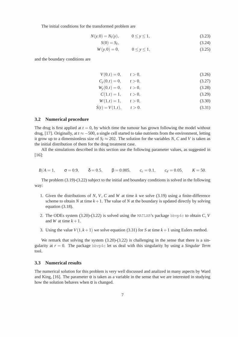
Figure 1: Evolution of the tumour radius for different values of α.

0 10 20 30 40 50 60 70 80 90 100−10

−8

−6

−4

−2

0

2

4

6

alpha

velo

city

at

the

bo

un

dar

y

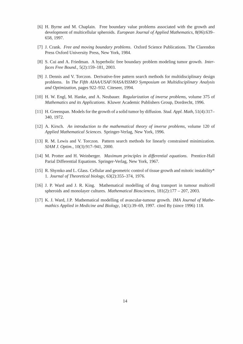
Figure 2: Velocity at the tumour’s boundary for a fixed time (t = 10) for different values ofα.

We are able to confirm thatα can, indeed, be considered ameasure of the treatment effectiveness.We plot how the radius of the tumour evolves in time when varying this parameter, as showed infigure 1.

We can observe that a valueα = 10 does not stop the growth of the tumour, although there is akilling cell process. However, ifα = 100 orα = 1000 the radius of the tumour decreases (of coursethe mass could never disappear because the drug does not act over the already formed necrotic core).

An interesting question to answer is:for which value ofα can be stated that tumour will decreasein size? That should be helpful, for example, w hen choosing some dosewhen the drug coefficientdiffusion and the initial spheroid size are known. To determine this value we take into account thevelocity in the boundary at a fixed time for different values of α. For example, in figure 2 we can seethat if we fix the non-dimensional timet = 10, the functionv(S(t), t) has a root inα ≈ 25.

The problem has also be solved for a different treatment protocol. We took a drug withα = 1000and provided it for some time intervals, so that the boundarycondition is the following:

w0(t) = 1, t ∈ [0,20),w0(t) = 0, t ∈ [20,50),w0(t) = 1, t ≥ 50.

8

0 10 20 30 40 50 60 70 80160

165

170

175

180

185

190

195

200

205

210

Time (adimensional)

Rad

ius

(ad

imen

sio

nal

)

Figure 3: Evolution of the tumour radius for a pulse-type drug provision.

In [16] the surviving fraction is plotted for a boundary condition similar to this one. In contrast,in figure 3 we plot the evolution of the tumour radius for this situation, which should be consideredwhen designing a treatment, because it is really important in the effectiveness-toxicity balance.

4 Inverse problem

The main idea of this section is to recover some of the parameters which appear in the mathemat-ical model, motivated in the lack of references that exist inliterature. In reality, some of them areunknown, especially in vivo.

We consider that the parameterα defined above is important because it provides a measure of thetreatment effectiveness. In particular, it can provide information about the drug diffusion coefficient,the optimal dose to get a desired effect or, eventually, Michaelis-Menten kinetics, see equation (2.21).

Thus, we are interested in the recovery of this parameter using available scans (MR images fromreal patients that could let us follow the tumour size evolution over time) or reliable measurementssuch as histological studies (obtained experimentally forin vitro cases). The data should be obtainedat different moments in time over a time interval of lenghtT. The inverse problem can be formulatedas follows:

Find a parameter value able to generate data that best match the available information over time0≤ t ≤ T.

Because of the nature of the mathematical model, we have to solve a PDE constrained optimiza-tion problem. The constraints are given by the model equations (2.1)-(2.14), which can be writtenin a short way asP (φ) = 0, whereP is the differential operator given by the set of equations andφ = (N,C,V,W).

4.1 The objective functional

We should construct an objective functional which gives us somedistancebetween the experimental(real) data and the solution of the system of PDEs for each value ofα.

First of all, it is important to decide which variables are capable to be measured experimentally.For instance, it is clear that the tumour radiusS(t) can be known at certain timestk, k= 1, ...,M. So,the first possibility for defining a functional could be

9

J(S;α) =∫ T

0[Sα(t)−S∗(t)]2dt, (4.1)

whereSα(t) is the radius evolution obtained solving the direct problemfor a certain value ofα andS∗(t) is the evolution measured experimentally (real data).

Other variable that could be measured is the concentration of living cells, via biomedical imaging.Thus, we are motivated to define a functional that reproducesin a better way the knowledge we haveabout the process, i.e.

J(N,S;α) =∫ 1

0

∫ T

0[Nα(y, t)−N∗(y, t)]2dtdy+µ

∫ T

0[Sα(t)−S∗(t)]2dt, (4.2)

whereNα(y, t) andN∗(y, t) are the living cell concentration for the direct problem solved with thevalue α and the real data, respectively (both of them in the domain[0,1]× [0,T]). The positiveconstantµ is introduced, as we shall see, to take into account the different order of magnitude betweenN andS.

So, the constrained optimization problem can be formulatedas

minα∈C

J(α),

s.t.P (φ) = 0,

whereC denotes the set ofadmissible valuesof α.We remark that, in general, there is a fundamental difference between the direct and the inverse

problems. In fact, the latter is usually ill-posed in the sense of existence, uniqueness and stability ofthe solution. This inconvenient is often treated by using some regularization techniques, [12, 10].

4.2 Discretization of the objective functional

Even if the functionsS(t) andN(y, t) are not known in their whole domains, it is sufficient to knowthe values that they take at several points (defining a convenient grid mesh fory andt).

First of all, suppose that we have experimental measurements of N andS at different timestk,k= 1, ...,M. That would give us temporal information about the variables.

On the other hand, the distribution of living cells depends also on the position along the tumour.A common techniche in medical imaging islandmark registration: landmarks are points placed atmeaningful parts of the tumour, with the intention of representing it as good as possible with a fewisolated points. Lety j , j = 1, ...,Q denote a set of points in the interval[0,1] that are chosen by anexpert. Note that the points should be chosen in the interval[0,S(t)], but for simplicity we will assumethat they are fixed in time.

Then, the objective functional (4.2) can be discretized as

J(N,S;α) =Q

∑j=1

M

∑k=1

[Nα(y j , tk)−N∗(y j , tk)]2+µ

M

∑k=1

[Sα(tk)−S∗(tk)]2dt. (4.3)

10

5 Numerical experiments

The pattern search method, [9]-[13], was employed to estimate the parameter of interest by minimiz-ing the objective functional. It is a direct method, i.e. a method that neither compute nor explicitlyapproximate derivatives ofJ. For this purpose we use the functionpattern search of MATLAB.

We study the functionals behaviour by solving some test cases. The living cell density and thetumour radius are generated via the forward problem. We showhere the results obtained by assuminga standard valueα = 1000. It seems that this value is quite reasonable, see [16],although in a nextstep we are trying to determine whether or not the dose considered is tolerable for a patient.

1. Model-generated data

Consider first an optimization problem that consist in minimizing the functional (4.3), whereN∗(y, t) andS∗(t) are generated via the forward model, for a choice of the modelparameterα = 1000.

Working with the functional (4.3) requires to define the landmark pointsy j and the timestkwhere the measurements are made. For simplicity, and to be consistent with the way we solvedthe direct problem, we took the same spatial grid for the landmarks, i.e. 30 equidistant points0 = y1 < ... < y30 = 1. Regarding to the time selection, it is apparent from the experimentsthat 20 time steps are enough to obtain the desired results, so we take 20 equidistant pointst1 < ... < t20. The factorµ is taken to be 1.

The idea of this test case is to investigate how close the original value of the parameter canbe retrieved. However, it is not a trivial one, because we do not know, for instance, if theoptimization problem has a solution or, in that case, if it isunique or if the method convergesto another local minima.

We emphasize we have run the algorithm several times using different initial random conditionsand in all cases the results were similar. They can be summarized in the following table:

• Stopping criteria:difference between two consecutive iterations lower than10−5

• Iterations/elapsed time:25/45 min

• Final point:α = 1001

• Functional final value:J(α) = 1.8871.10−4

2. Model-generated data with5%of random noise

It is well known that the presence of noise in the data may imply the appearance of strongnumerical instabilities in the solution of an inverse problem, [5].

The outputs of the detectors and the experimental equipmentwhere the variablesN∗ andS∗ aremeasured are often affected by perturbations, usually random ones. As stated in [3], it is ingeneral valid to consider a 5% of random noise.

The functional (4.3) is the same used for case 1, except from the constantµ. It was clear fromnumerical experiments that the factorµ= 1 was not suitable for this case, as it is showed infigures 4 and 5, where we can see that the order of magnitude between both terms in theobjective functional is different. Indeed, in the case of the living cell density, we can see thatboth lines are almost indistinguishable. By a trial and error procedure, we determined thatµ= 10−4 is a suitable factor.

Again, starting with different points, the results of the procedure are the following:

11

0 10 20 30 40 50 60 70 80 90 100160

165

170

175

180

185

190

195

200

205

210

Time (adimensional)

Rad

ius

(ad

imen

sio

nal

)

Figure 4: Evolution of the tumour radius without (red line) and with 5% random noise (blue line).

100 110 120 130 140 150 160 170 180 190 2000

0.1

0.2

0.3

0.4

0.5

0.6

0.7

0.8

0.9

1

Radius (adimensional)

Liv

ing

cel

l den

sity

Figure 5: Living cell distribution without (red line) and with 5% random noise (blue line), for theinitial time.

12

• Stopping criteria:difference between two consecutive iterations lower than10−5

• Iterations/elapsed time:24/36 min

• Final point:α = 992.97

• Functional final value:J(α) = 0.100886

6 Conclusions and future work

A simple methodology was developed for the estimation of biochemical parameters involved in thegrowth of an avascular tumour using data that could be obtained from medical imaging. The inverseproblem has been solved using the Pattern Search algorithm,coupled with a finite different schemeand a boundary value problem solver for the resolution of thedirect problem. The presented resultsdemonstrate the feasibility of the proposed methodology. Even in the case when 5% of noise wasadded to the input data the methodology estimates the desired parameter with very good accuracy

According to the results, this methodology can help to estimate several chemical/biological pa-rameters involved in the process (diffusion coefficient, mitosis and death rates, Michaelis-Mentenconstants, etc.) that could be useful and important to studyfor the design of a treatment procedure.As future work we plan to recover more parameters involved inthe model, and focus on the regular-ization of the problem considering different regularization methods and iterative algorithms. In orderto solve the optimization problem, we will use an algorithm that take into account the derivative ofthe functional like the conjugate gradient method.

In addition, we are trying to use these optimization ideas towork with vascular tumour’s model.That will surely give a more realistic idea of a chemotherapeutic treatment and its protocol.

Acknowledgments

The work of the authors was partially supported by grants from CONICET, SECYT-UNC and PICT-FONCYT.

References

[1] J. Adam and N. Bellomo.A survey of models for tumor immune systems dynamics. Modelingand simulation in science, engineering & technology. Birkhauser, 1997.

[2] J. A. Adam. A simplified mathematical model of tumor growth. Mathematical Biosciences,81(2):229 – 244, 1986.

[3] J. Agnelli, A. Barrea, and C. Turner. Tumor location and parameter estimation by thermography.Mathematical and Computer Modelling, 53(7-8):1527 – 1534, 2011. Mathematical Methodsand Modelling of Biophysical Phenomena.

[4] B. V. Bazaliy and A. Friedman. A free boundary problem foran elliptic-parabolic system:application to a model of tumor growth.Comm. Partial Differential Equations, 28(3-4):517–560, 2003.

[5] M. Bertero and M. Piana. Inverse problems in biomedical imaging: modeling and methods ofsolution.Complex Systems in Biomedicine, pages 1–33, 2006.

13

[6] H. Byrne and M. Chaplain. Free boundary value problems associated with the growth anddevelopment of multicellular spheroids.European Journal of Applied Mathematics, 8(06):639–658, 1997.

[7] J. Crank. Free and moving boundary problems. Oxford Science Publications. The ClarendonPress Oxford University Press, New York, 1984.

[8] S. Cui and A. Friedman. A hyperbolic free boundary problem modeling tumor growth.Inter-faces Free Bound., 5(2):159–181, 2003.

[9] J. Dennis and V. Torczon. Derivative-free pattern search methods for multidisciplinary designproblems. InThe Fifth AIAA/USAF/NASA/ISSMO Symposium on Multidisciplinary Analysisand Optimization, pages 922–932. Citeseer, 1994.

[10] H. W. Engl, M. Hanke, and A. Neubauer.Regularization of inverse problems, volume 375 ofMathematics and its Applications. Kluwer Academic Publishers Group, Dordrecht, 1996.

[11] H. Greenspan. Models for the growth of a solid tumor by diffusion.Stud. Appl. Math, 51(4):317–340, 1972.

[12] A. Kirsch. An introduction to the mathematical theory of inverse problems, volume 120 ofApplied Mathematical Sciences. Springer-Verlag, New York, 1996.

[13] R. M. Lewis and V. Torczon. Pattern search methods for linearly constrained minimization.SIAM J. Optim., 10(3):917–941, 2000.

[14] M. Protter and H. Weinberger.Maximum principles in differential equations. Prentice-HallParial Differential Equations. Springer-Verlag, New York, 1967.

[15] R. Shymko and L. Glass. Cellular and geometric control of tissue growth and mitotic instability*1. Journal of Theoretical biology, 63(2):355–374, 1976.

[16] J. P. Ward and J. R. King. Mathematical modelling of drugtransport in tumour multicellspheroids and monolayer cultures.Mathematical Biosciences, 181(2):177 – 207, 2003.

[17] K. J. Ward, J.P. Mathematical modelling of avascular-tumour growth.IMA Journal of Mathe-mathics Applied in Medicine and Biology, 14(1):39–69, 1997. cited By (since 1996) 118.

14

A parameter estimation problem for a tumour growth model .

D. A. Knopoff, D. R. Fernandez, G. A. Torres and C. V. Turner∗

FaMAF, Universidad Nacional de Cordoba - CIEM-CONICET. Cordoba, Argentina.

Abstract

In this paper we present a method for estimating unknown parameters that appear on anavascular, spheric tumour growth model. The model for the tumour is based on nutrient drivengrowth of a continuum of live cells, whose birth and death generate volume changes describedby a velocity field. The drug is applied externally, and is assumed to be a diffusible substancecapable of killing cells.

The model consists on a coupled system of partial differential equations which is solvednumerically. As the domain on which the equations are definedis the tumour, that changes in sizeover time, the problem can be formulated as a moving boundaryone.

After solving the forward problem properly, we are concerned in using the model for theestimation of parameters, by fitting the numerical solutionwith real data. We define a functionalto compare both of them and we use the pattern search method for minimizing it, obtaining goodaccuracy for the recovery of a few parameters.

Keywords: avascular tumour, constrained optimization, inverse problem, mathematical modeling.

1 Introduction.

The interest for research in modeling cancer has grown enormously over the last decades, [1, 2].Pioneers have been, for example, [11, 15], where the first spatio-temporal models of an avascularmulticellular spheroid’s (MCS) growth have been developed. The study of MCS is interesting be-cause they provide the best insight into the effectiveness of chemotherapeutic drugs on tumours invivo, and their behaviour can be studied experimentally (invitro) by controlling environmental con-ditions in which they grow: for example, the radii of the tumour can be monitored by changing thechemotherapeutic drug or oxygen levels.

In addition, another variables can be measured. If possible, experimentalists can get informationabout the distribution of substances within the tumour. Moreover, via medical imaging or histologicalcuts, they can also get data about the density of the different kind of cells conforming it: proliferating,quiescent, necrotic.

That is why in this general approach of modeling the key variables are the tumour size (radius)and the concentration within the tumour of growth-rate limiting diffusible chemicals (nutrients suchas oxygen or glucose or a chemotherapeutic drug). Since the tumour changes in size over time, thedomain on which the models are formulated must be determinedas part of the solution process, givinga vast class of moving boundary problems, [6, 7].

In this article, we propose a framework for estimating unknown parameters via PDE-constrainedoptimization, following the PDE-based model by Ward and King, [16]. In this approach, avascular

∗E-mail address: knopoff@famaf.unc.edu.ar, dfernandez@famaf.unc.edu.ar, torres@gmail.com,turner@famaf.unc.edu.ar

1

tumour growth is modeled via a coupled nonlinear system of differential equations, which make thenumerical solution procedure quite challenging.

We are concerned with developing a robust PDE-constrained formulation that let us find the bestset of parameters of a tumour growth model that fits patient orexperimental data. We choose theparameters that should be of applied interest and try to obtain them by defining a functional to beminimized.

The paper is organized as follows: section 2 introduces the tumour growth model (forward prob-lem). Section 3 shows the numerical solution of the forward problem and checks its accuracy byproving some theoretical results. Section 4 introduces theinverse problem approach, by defining thefunctional to be minimized. Finally, in section 5 the numerical procedure to solve the inverse problemis discussed.

2 Mathematical model.

We consider the model proposed by Ward and King in [16]. The tumour is a spheroid which consistsof a continuum of living cells, in one of two states: live or dead. The rates of birth and death dependon the nutrient and chemotherapeutic drug concentration. It is supposed that those processes generatevolume changes, leading to cell movement described by a velocity field. The system of equations tobe studied is:

∂n∂t

+1r2

∂(r2vn)∂r

= [km(c)−kd(c)−KG(km(c))w]n, (2.1)

∂c∂t

+1r2

∂(r2vc)∂r

=Dr2

∂∂r

(r2 ∂c

∂r

)−βkm(c)n, (2.2)

1r2

∂(r2v)∂r

= [VLkm(c)− (VL −VD){kd(c)+KG(km(c))w}]n, (2.3)

∂w∂t

+1r2

∂(r2vw)∂r

=Dw

r2

∂∂r

(r2 ∂w

∂r

)−

Kω

G(km(c))wn, (2.4)

where the dependent variablesn, c, v and w are the live cell density (cells/unit volume), nutrientconcentration, velocity and drug concentration, respectively. As it is described in [16], equation (2.1)states that the rate of change ofn is dependent on the difference between the birthkm(c) and deathkd(c) rates, where this one is either natural (as described in [17]) or due to the drug effects, at a rateKG(km(c))w. The functonskm andkd are taken to be generalised Michaelis-Menten kinetics withexponent 1, i.e.

km(c) = A

(c

cc+c

), (2.5)

kd(c) = B

(1−σ

ccd +c

). (2.6)

The constantK is the maximum possible rate of drug induced cell death. The constantsA, B andσare positive parameters of the Michaelis-Menten kinetics,while cc andcd are critical concentrations.G(km(c)) is a function that represents the dependence between drug action and cell-cycle. As it isconsidered in [16] it is a good idea to choose a linear dependence, giving

G(km(c)) = km(c)/A.

2

Equation (2.2) states that the nutrient is consumed at a rateproportional to the rate of mitosis,and its diffusion is described by Ficks law. Equation (2.3) states that the rate of volume change isgiven by the difference in volume generated via birth from that lost by death (it is assumed that a livecell occupies a volumeVL that is twice the volume of a death cellVD). The diffusion of the drug isdescribed also by Ficks law, and it is assumed that it is degraded only when it attacks a living cell,giving a maximum degradation rateK/ω. ω is a dimensionless constant that can be interpreted as ameasure of the drugs effectiveness, as explained in [16], with increasingω implying that less drugis consumed to produce the same effects during the killing process. These considerations lead toequation (2.4).

2.1 Moving boundary problem

As it has been mentioned, the tumour is assumed to be a spheroid that exhibits radial simmetry. Thatis why, not only the state variablesn, c, v andw are important, but the outer tumour radius is also akey variable to be determined. Since the tumour changes in size over time, the domains on which themodels are formulated (and the PDEs are valid) must be determined as part of the solution.

Let S(t) be the tumour radius at timet. So, if we suppose that the treatment begins at timet = 0,in which the tumour has a radiusSI , with living cell density and nutrient concentration distributionsnI (r) andcI (r), respectively, then the initial conditions of the problem can be formulated as

n(r,0) = nI (r), (2.7)

c(r,0) = cI (r), (2.8)

w(r,0) = 0, (2.9)

S(0) = SI . (2.10)

Because symmetry is assumed about the tumour center, there is no flux there. That is why, asboundary conditions aboutr = 0, are taken:

∂c∂r

(0, t) = 0, (2.11)

v(0, t) = 0, (2.12)∂w∂r

(0, t) = 0. (2.13)

Moreover, on the external boundary (which is also the boundary of the complement of the tumouras a subset of the body), the following conditions are taken:

c(S(t), t) = c0, (2.14)dSdt

= v(S(t), t), (2.15)

w(S(t), t) = w0(t), (2.16)

wherec0 andw0(t) are external nutrient and drug concentrations, respectively. The functionw0(t)depends on the chemotherapeutic protocol. In our simulations it will be considered as a constant thatdoes not depend ont. However, other functions may be adopted, for example in section 3 we showan example in which drug is provided for some intervals of time, but not for other ones.

3

2.2 Nondimensionalisation

Before analysing the model equations, we re-scale the mathematical model in the following way,denoting non-dimensional variables with bars:

n=VLn; c= c/c0; v= v/r0A; t = At r = r/r0; S= S/r0; w= w/W0

wherer0 = (3VL/4π)1/3 is the radius of a single cell andW0 is a suitable reference drug concentration(typically W0 = max(w0(t))).

It is important to remark that inherent in this problem are two timescales: the tumour growthtimescale (≈ 1 day) and the much shorter drug and nutrient diffusions (≈ 1 min). That is why,following [2, 1, 16, 6] we adopt a quasi-steady assumption inthe nutrient and drug equations.

Following [16], and relabeling the variables with bar againwithout it, these rescalings lead to thefollowing system of differential equations:

∂n∂t

+v∂n∂r

= [a(c,w)−b(c,w)n]n, (2.17)

1r2

∂∂r

(r2 ∂c

∂r

)= k(c)n, (2.18)

1r2

∂(r2v)∂r

= b(c,w)n, (2.19)

1r2

∂∂r

(r2∂w

∂r

)=

Kα

km(c)wn, (2.20)

where

α = ωDwVLW0/Ar20, (2.21)

K = KW0/A,

a(c,w) =1A[km(c)−kd(c)−KG(km(c))w],

b(c,w) =1A{km(c)− (1−δ)[kd(c)−KG(km(c))w]},

k(c) = βkm(c)/A,

with δ =VD/VL and(β) = r20βA/VLc0D.

We note that theconstantα defined above comprises many model parameters that should beinteresting to know exactly. It will be of great importance in the next sections, whereα will beconsidered as a key parameter of the problem.

Also, it is worth saying that rigorous mathematical analysis including existence, uniqueness, andstability theorems, as well as properties of the free boundaries for similar tumour growth models inwhich different kind of PDEs are combined, have been obtained, [4] and [8].

4

3 Numerical solution of the forward problem

After the assumptions made in the previous section, we have to solve the following system of PDEs:

nt +vnr = [a(c,w)−b(c,w)n]n 0< r ≤ S(t), t > 0, (3.1)

vr +2r

v= b(c,w)n 0< r ≤ S(t), t > 0, (3.2)

crr +2r

cr = k(c)n 0< r ≤ S(t), t > 0, (3.3)

wrr +2r

wr =Kα

km(c)w 0< r ≤ S(t), t > 0. (3.4)

The initial conditions att = 0 are

n(r,0) = nI (r), (3.5)

S(0) = SI , (3.6)

w(r,0) = 0, (3.7)

and the boundary conditions are

v(0, t) = 0, (3.8)

cr(0, t) = 0, (3.9)

wr(0, t) = 0, (3.10)

c(S(t), t) = 1, (3.11)

w(S(t), t) = 1, (3.12)

S(t) = v(S(t), t). (3.13)

It is important to remark that the density of living cells in the boundary,n(S(t), t), can be calcu-lated explicitly. Indeed, consider equation (3.1) and notethat, using the chain rule, the total variationof n in time is

dndt

=∂n∂t

+∂n∂r

drdt

. (3.14)

At the point(S(t), t) the expressiondrdt is equal tov(S(t), t). So, substitution in (3.1 ) gives

dndt

(S(t), t) = [a(1,1)−b(1,1)n(S(t), t)]n(S(t), t),

wherea(1,1) andb(1,1) are the corresponding values of the functionsa andb on the boundary at anytime. The last equation is a separable ODE, that can be transformed into

dn∗

[a∗−b∗n∗]n∗= dt, (3.15)

where for simplicity we wrotea∗ = a(1,1), b∗ = b(1,1) andn∗ = n(S(t), t).Now, we use expansion into simple fractions:

5

1(a∗−b∗n∗)n∗

=b∗

a∗1

a∗−b∗n∗+

1a∗

1n∗

. (3.16)

Combining equations (3.15) and (3.16) and integrating overtime we get

∫ t

0dt =

∫ n(S(t),t)

1

dn∗

(a∗−b∗n∗)n∗= ln

((a∗−b∗)n(S(t), t)a∗−b∗n(S(t), t)

). (3.17)

Finally, solving forn on the boundary, we obtain

n(S(t), t) =a∗ea∗t

a∗−b∗+b∗ea∗t . (3.18)

Equation (3.18) is not only an elegant analytical result, but also it will become of really importancewhen calculating numerically the value ofn in the boundary. As we shall see, when defining thespatial grid to solve equation (3.1) with a forward finite difference scheme, for each pointr j of thegrid we will need to take also the pointr j+1 but that is impossible in the last point of the grid, sayS(t)

3.1 Fixed domain method

The first step for solving this moving boundary problem will be transforming the original domain toa fixed one, i.e., re-writing the whole system for the change of coordinatesy= r/S(t). In this way,the spatial domain will be the interval[0,1].

Observation 3.1 If r = yS(t), then drdy = S(t) and dr

dt = yS(t).

We briefly illustrate the way in which the new equations are obtained, using (3.1).Let N(y, t)

.= n(r, t) = n(yS(t), t). Differentiating this expression respect toy, we obtain

Ny = nr ry+ntty = nrS(t),

and thennr =Ny

S .And differentiation respect tot gives

Nt = nrdrdt

+nt ,

and so we deduce thatnt = Nt −Ny

S yS.Substitution in (3.1) gives

Nt −SS

yNy+VS

Ny = N[a(C)−b(C)N]N 0< r ≤ 1, t > 0. (3.19)

The same procedure is applied to the other equations, and we obtain

Cyy+2yCy = k(C)S2N, (3.20)

Vy+2yV = b(C)NS, (3.21)

Wyy+2yWy =

Kα

km(C)S2WN. (3.22)

6

The initial conditions for the transformed problem are

N(y,0) = NI(y), 0≤ y≤ 1, (3.23)

S(0) = SI , (3.24)

W(y,0) = 0, 0≤ y≤ 1, (3.25)

and the boundary conditions are

V(0, t) = 0, t > 0, (3.26)

Cy(0, t) = 0, t > 0, (3.27)

Wy(0, t) = 0, t > 0, (3.28)

C(1, t) = 1, t > 0, (3.29)

W(1, t) = 1, t > 0, (3.30)

S(t) =V(1, t), t > 0. (3.31)

3.2 Numerical procedure

The drug is first applied att = 0, by which time the tumour has grown following the model withoutdrug, [17]. Originally, att ≈−500, a single cell started to take nutrients from the environment, lettingit grow up to a dimensionless size ofSI ≈ 202. The solution for the variablesN, C andV is taken asthe initial distribution of them for the drug treatment case.

All the simulations described in this section use the following parameter values, as suggested in[16]:

B/A= 1, σ = 0.9, δ = 0.5, β = 0.005, cc = 0.1, cd = 0.05, K = 50.

The problem (3.19)-(3.22) subject to the initial and boundary conditions is solved in the followingway:

1. Given the distributions ofN, V, C andW at timek we solve (3.19) using a finite-differencescheme to obtainN at timek+1. The value ofN at the boundary is updated directly by solvingequation (3.18).

2. The ODEs system (3.20)-(3.22) is solved using theMATLAB’s packagebbvp4c to obtainC, VandW at timek+1.

3. Using the valueV(1,k+1) we solve equation (3.31) forSat timek+1 using Eulers method.

We remark that solving the system (3.20)-(3.22) is challenging in the sense that there is a sin-gularity at r = 0. The packagebbvp4c let us deal with this singularity by using aSingular Termtool.

3.3 Numerical results

The numerical solution for this problem is very well discussed and analized in many aspects by Wardand King, [16]. The parameterα is taken as a variable in the sense that we are interested in studyinghow the solution behaves whenα is changed.

7

0 10 20 30 40 50 60 70 80186

188

190

192

194

196

198

200

202

204

206

100*time (adimensional)

tu

mo

r ra

diu

s (a

dim

ensi

on

al)

alfa = 10 (non−effective treatment)alfa = 100 (effective treatment)alfa = 1000 (effective treatment)

Figure 1: Evolution of the tumour radius for different values of α.

0 10 20 30 40 50 60 70 80 90 100−10

−8

−6

−4

−2

0

2

4

6

alpha

velo

city

at

the

bo

un

dar

y

Figure 2: Velocity at the tumour’s boundary for a fixed time (t = 10) for different values ofα.

We are able to confirm thatα can, indeed, be considered ameasure of the treatment effectiveness.We plot how the radius of the tumour evolves in time when varying this parameter, as showed infigure 1.

We can observe that a valueα = 10 does not stop the growth of the tumour, although there is akilling cell process. However, ifα = 100 orα = 1000 the radius of the tumour decreases (of coursethe mass could never disappear because the drug does not act over the already formed necrotic core).

An interesting question to answer is:for which value ofα can be stated that tumour will decreasein size? That should be helpful, for example, w hen choosing some dosewhen the drug coefficientdiffusion and the initial spheroid size are known. To determine this value we take into account thevelocity in the boundary at a fixed time for different values of α. For example, in figure 2 we can seethat if we fix the non-dimensional timet = 10, the functionv(S(t), t) has a root inα ≈ 25.

The problem has also be solved for a different treatment protocol. We took a drug withα = 1000and provided it for some time intervals, so that the boundarycondition is the following:

w0(t) = 1, t ∈ [0,20),w0(t) = 0, t ∈ [20,50),w0(t) = 1, t ≥ 50.

8

0 10 20 30 40 50 60 70 80160

165

170

175

180

185

190

195

200

205

210

Time (adimensional)

Rad

ius

(ad

imen

sio

nal

)

Figure 3: Evolution of the tumour radius for a pulse-type drug provision.

In [16] the surviving fraction is plotted for a boundary condition similar to this one. In contrast,in figure 3 we plot the evolution of the tumour radius for this situation, which should be consideredwhen designing a treatment, because it is really important in the effectiveness-toxicity balance.

4 Inverse problem

The main idea of this section is to recover some of the parameters which appear in the mathemat-ical model, motivated in the lack of references that exist inliterature. In reality, some of them areunknown, especially in vivo.

We consider that the parameterα defined above is important because it provides a measure of thetreatment effectiveness. In particular, it can provide information about the drug diffusion coefficient,the optimal dose to get a desired effect or, eventually, Michaelis-Menten kinetics, see equation (2.21).

Thus, we are interested in the recovery of this parameter using available scans (MR images fromreal patients that could let us follow the tumour size evolution over time) or reliable measurementssuch as histological studies (obtained experimentally forin vitro cases). The data should be obtainedat different moments in time over a time interval of lenghtT. The inverse problem can be formulatedas follows:

Find a parameter value able to generate data that best match the available information over time0≤ t ≤ T.

Because of the nature of the mathematical model, we have to solve a PDE constrained optimiza-tion problem. The constraints are given by the model equations (2.1)-(2.14), which can be writtenin a short way asP (φ) = 0, whereP is the differential operator given by the set of equations andφ = (N,C,V,W).

4.1 The objective functional

We should construct an objective functional which gives us somedistancebetween the experimental(real) data and the solution of the system of PDEs for each value ofα.

First of all, it is important to decide which variables are capable to be measured experimentally.For instance, it is clear that the tumour radiusS(t) can be known at certain timestk, k= 1, ...,M. So,the first possibility for defining a functional could be

9

J(S;α) =∫ T

0[Sα(t)−S∗(t)]2dt, (4.1)

whereSα(t) is the radius evolution obtained solving the direct problemfor a certain value ofα andS∗(t) is the evolution measured experimentally (real data).

Other variable that could be measured is the concentration of living cells, via biomedical imaging.Thus, we are motivated to define a functional that reproducesin a better way the knowledge we haveabout the process, i.e.

J(N,S;α) =∫ 1

0

∫ T

0[Nα(y, t)−N∗(y, t)]2dtdy+µ

∫ T

0[Sα(t)−S∗(t)]2dt, (4.2)

whereNα(y, t) andN∗(y, t) are the living cell concentration for the direct problem solved with thevalue α and the real data, respectively (both of them in the domain[0,1]× [0,T]). The positiveconstantµ is introduced, as we shall see, to take into account the different order of magnitude betweenN andS.

So, the constrained optimization problem can be formulatedas

minα∈C

J(α),

s.t.P (φ) = 0,

whereC denotes the set ofadmissible valuesof α.We remark that, in general, there is a fundamental difference between the direct and the inverse

problems. In fact, the latter is usually ill-posed in the sense of existence, uniqueness and stability ofthe solution. This inconvenient is often treated by using some regularization techniques, [12, 10].

4.2 Discretization of the objective functional

Even if the functionsS(t) andN(y, t) are not known in their whole domains, it is sufficient to knowthe values that they take at several points (defining a convenient grid mesh fory andt).

First of all, suppose that we have experimental measurements of N andS at different timestk,k= 1, ...,M. That would give us temporal information about the variables.

On the other hand, the distribution of living cells depends also on the position along the tumour.A common techniche in medical imaging islandmark registration: landmarks are points placed atmeaningful parts of the tumour, with the intention of representing it as good as possible with a fewisolated points. Lety j , j = 1, ...,Q denote a set of points in the interval[0,1] that are chosen by anexpert. Note that the points should be chosen in the interval[0,S(t)], but for simplicity we will assumethat they are fixed in time.

Then, the objective functional (4.2) can be discretized as

J(N,S;α) =Q

∑j=1

M

∑k=1

[Nα(y j , tk)−N∗(y j , tk)]2+µ

M

∑k=1

[Sα(tk)−S∗(tk)]2dt. (4.3)

10

5 Numerical experiments

The pattern search method, [9]-[13], was employed to estimate the parameter of interest by minimiz-ing the objective functional. It is a direct method, i.e. a method that neither compute nor explicitlyapproximate derivatives ofJ. For this purpose we use the functionpattern search of MATLAB.

We study the functionals behaviour by solving some test cases. The living cell density and thetumour radius are generated via the forward problem. We showhere the results obtained by assuminga standard valueα = 1000. It seems that this value is quite reasonable, see [16],although in a nextstep we are trying to determine whether or not the dose considered is tolerable for a patient.

1. Model-generated data

Consider first an optimization problem that consist in minimizing the functional (4.3), whereN∗(y, t) andS∗(t) are generated via the forward model, for a choice of the modelparameterα = 1000.

Working with the functional (4.3) requires to define the landmark pointsy j and the timestkwhere the measurements are made. For simplicity, and to be consistent with the way we solvedthe direct problem, we took the same spatial grid for the landmarks, i.e. 30 equidistant points0 = y1 < ... < y30 = 1. Regarding to the time selection, it is apparent from the experimentsthat 20 time steps are enough to obtain the desired results, so we take 20 equidistant pointst1 < ... < t20. The factorµ is taken to be 1.

The idea of this test case is to investigate how close the original value of the parameter canbe retrieved. However, it is not a trivial one, because we do not know, for instance, if theoptimization problem has a solution or, in that case, if it isunique or if the method convergesto another local minima.

We emphasize we have run the algorithm several times using different initial random conditionsand in all cases the results were similar. They can be summarized in the following table:

• Stopping criteria:difference between two consecutive iterations lower than10−5

• Iterations/elapsed time:25/45 min

• Final point:α = 1001

• Functional final value:J(α) = 1.8871.10−4

2. Model-generated data with5%of random noise

It is well known that the presence of noise in the data may imply the appearance of strongnumerical instabilities in the solution of an inverse problem, [5].

The outputs of the detectors and the experimental equipmentwhere the variablesN∗ andS∗ aremeasured are often affected by perturbations, usually random ones. As stated in [3], it is ingeneral valid to consider a 5% of random noise.

The functional (4.3) is the same used for case 1, except from the constantµ. It was clear fromnumerical experiments that the factorµ= 1 was not suitable for this case, as it is showed infigures 4 and 5, where we can see that the order of magnitude between both terms in theobjective functional is different. Indeed, in the case of the living cell density, we can see thatboth lines are almost indistinguishable. By a trial and error procedure, we determined thatµ= 10−4 is a suitable factor.

Again, starting with different points, the results of the procedure are the following:

11

0 10 20 30 40 50 60 70 80 90 100160

165

170

175

180

185

190

195

200

205

210

Time (adimensional)

Rad

ius

(ad

imen

sio

nal

)

Figure 4: Evolution of the tumour radius without (red line) and with 5% random noise (blue line).

100 110 120 130 140 150 160 170 180 190 2000

0.1

0.2

0.3

0.4

0.5

0.6

0.7

0.8

0.9

1

Radius (adimensional)

Liv

ing

cel

l den

sity

Figure 5: Living cell distribution without (red line) and with 5% random noise (blue line), for theinitial time.

12

• Stopping criteria:difference between two consecutive iterations lower than10−5

• Iterations/elapsed time:24/36 min

• Final point:α = 992.97

• Functional final value:J(α) = 0.100886

6 Conclusions and future work

A simple methodology was developed for the estimation of biochemical parameters involved in thegrowth of an avascular tumour using data that could be obtained from medical imaging. The inverseproblem has been solved using the Pattern Search algorithm,coupled with a finite different schemeand a boundary value problem solver for the resolution of thedirect problem. The presented resultsdemonstrate the feasibility of the proposed methodology. Even in the case when 5% of noise wasadded to the input data the methodology estimates the desired parameter with very good accuracy

According to the results, this methodology can help to estimate several chemical/biological pa-rameters involved in the process (diffusion coefficient, mitosis and death rates, Michaelis-Mentenconstants, etc.) that could be useful and important to studyfor the design of a treatment procedure.As future work we plan to recover more parameters involved inthe model, and focus on the regular-ization of the problem considering different regularization methods and iterative algorithms. In orderto solve the optimization problem, we will use an algorithm that take into account the derivative ofthe functional like the conjugate gradient method.

In addition, we are trying to use these optimization ideas towork with vascular tumour’s model.That will surely give a more realistic idea of a chemotherapeutic treatment and its protocol.

Acknowledgments

The work of the authors was partially supported by grants from CONICET, SECYT-UNC and PICT-FONCYT.

References

[1] J. Adam and N. Bellomo.A survey of models for tumor immune systems dynamics. Modelingand simulation in science, engineering & technology. Birkhauser, 1997.

[2] J. A. Adam. A simplified mathematical model of tumor growth. Mathematical Biosciences,81(2):229 – 244, 1986.

[3] J. Agnelli, A. Barrea, and C. Turner. Tumor location and parameter estimation by thermography.Mathematical and Computer Modelling, 53(7-8):1527 – 1534, 2011. Mathematical Methodsand Modelling of Biophysical Phenomena.

[4] B. V. Bazaliy and A. Friedman. A free boundary problem foran elliptic-parabolic system:application to a model of tumor growth.Comm. Partial Differential Equations, 28(3-4):517–560, 2003.

[5] M. Bertero and M. Piana. Inverse problems in biomedical imaging: modeling and methods ofsolution.Complex Systems in Biomedicine, pages 1–33, 2006.

13

[6] H. Byrne and M. Chaplain. Free boundary value problems associated with the growth anddevelopment of multicellular spheroids.European Journal of Applied Mathematics, 8(06):639–658, 1997.

[7] J. Crank. Free and moving boundary problems. Oxford Science Publications. The ClarendonPress Oxford University Press, New York, 1984.

[8] S. Cui and A. Friedman. A hyperbolic free boundary problem modeling tumor growth.Inter-faces Free Bound., 5(2):159–181, 2003.

[9] J. Dennis and V. Torczon. Derivative-free pattern search methods for multidisciplinary designproblems. InThe Fifth AIAA/USAF/NASA/ISSMO Symposium on Multidisciplinary Analysisand Optimization, pages 922–932. Citeseer, 1994.

[10] H. W. Engl, M. Hanke, and A. Neubauer.Regularization of inverse problems, volume 375 ofMathematics and its Applications. Kluwer Academic Publishers Group, Dordrecht, 1996.

[11] H. Greenspan. Models for the growth of a solid tumor by diffusion.Stud. Appl. Math, 51(4):317–340, 1972.

[12] A. Kirsch. An introduction to the mathematical theory of inverse problems, volume 120 ofApplied Mathematical Sciences. Springer-Verlag, New York, 1996.

[13] R. M. Lewis and V. Torczon. Pattern search methods for linearly constrained minimization.SIAM J. Optim., 10(3):917–941, 2000.

[14] M. Protter and H. Weinberger.Maximum principles in differential equations. Prentice-HallParial Differential Equations. Springer-Verlag, New York, 1967.

[15] R. Shymko and L. Glass. Cellular and geometric control of tissue growth and mitotic instability*1. Journal of Theoretical biology, 63(2):355–374, 1976.

[16] J. P. Ward and J. R. King. Mathematical modelling of drugtransport in tumour multicellspheroids and monolayer cultures.Mathematical Biosciences, 181(2):177 – 207, 2003.

[17] K. J. Ward, J.P. Mathematical modelling of avascular-tumour growth.IMA Journal of Mathe-mathics Applied in Medicine and Biology, 14(1):39–69, 1997. cited By (since 1996) 118.

14