Embed Size (px)
Citation preview
1
Sentiment-Based Commercial Real Estate Forecasting with Google
Search Volume Data
Marian Alexander Dietzel, [email protected]
IRE|BS – International Real Estate Business School, University of Regensburg
Nicole Braun, [email protected]
IRE|BS – International Real Estate Business School, University of Regensburg
Wolfgang Schaefers, [email protected]
IRE|BS – International Real Estate Business School, University of Regensburg
2
Sentiment-Based Commercial Real Estate Forecasting with Google
Search Volume Data
Abstract
Purpose – This article examines internet search query data provided by ‘Google Trends’,
with respect to its ability to serve as a sentiment indicator and improve commercial real estate
forecasting models for transactions and price indices.
Methodology – The study uses data from CoStar the largest data providers of US commercial
real estate repeat sales indices. We design three groups of models: baseline models including
fundamental macro data only, those including Google data only and models combining both
sets of data.
One-month-ahead forecasts based on VAR models are conducted to compare the forecast
accuracy of the models.
Findings – The empirical results show that all models augmented with Google data,
combining both macro and search data, significantly outperform baseline models which
abandon internet search data.
Models based on Google data alone, outperform the baseline models in all cases.
The models achieve a reduction over the baseline models of the mean squared forecasting
error (MSE) for transactions and prices of up to 35% and 54% respectively.
Practical Implications – The results suggest that Google data can serve as an early market
indicator. The findings of this study suggest that the inclusion of Google search data in
forecasting models can improve forecast accuracy significantly. This implies that commercial
real estate forecasters should consider incorporating this free and timely data set into their
market forecasts or when performing plausibility checks for future investment decisions.
Originality – This is the first paper applying Google search query data to the commercial real
estate sector.
Keywords Forecasting, Commercial Real Estate, Investment Process, Google Trends, Search
Query Data, Sentiment, Prices, Transactions
Paper type Research paper

3
1. Introduction
Among others, Brooks and Tsolacos (2010) emphasise the importance of good forecasts for
the commercial real estate industry. There are fewer commercial properties than residential
buildings, but the former are usually of much higher value per unit. They form a
heterogeneous asset class, as they differ significantly in size, value and across sectors (retail,
office, industrial etc.), which makes them more difficult to compare among each other. As
opposed to the typical house buyer, commercial real estate buyers and sellers are
predominately professionals aiming to maximise their income.
Baum (2009) stresses the importance of forecasts, as real estate investors are interested in
what property type/market develops better than others, when it comes to selecting future
investments. Institutional investors, like insurance companies or property funds, usually have
a specific investment horizon in mind when allocating their funds. Hence, they produce
implicit and explicit forecasts about the performance of property markets across different
regions and sectors. Real estate consultancies publish market reports, in which they give an
outlook of market activity and movement. Property developers are particularly interested in
the future development of rents and prices, when setting up feasibility studies. When making
credit-approval decisions, banks and other real estate financers are interested in which
direction a market moves.
While homes serve either as self-owned accommodation or income-producing assets,
commercial properties usually serve only as the latter. This is particularly evident in periods
where, for example, sale-and-lease-back deals are fashionable, which leads to a reduction in
the share of users owning their own commercial property.
These unique attributes of commercial property cause the market to behave differently from
the housing market, which makes commercial real estate markets a special case in terms of
forecasting.
Although the literature on commercial real estate forecasting is not as comprehensive as for
housing, there are nonetheless many studies investigating the prediction of market behaviour.
Wheaton (1987) and Malizia (1991) focus on long-term relationships between the demand
and supply sides of commercial real estate markets and relate this to fundamental market
factors. MacKinnon and Al Zaman (2009) also take a closer look at the long-term effects of
return predictability and long-horizon asset allocations. Ghysels et al. (2007), on the other
hand, conclude that fundamental economic indicators “[…] cannot fully account for future
movements in returns”. This implies that there are unobservable factors influencing the
market, which are not captured by fundamentals.
Clayton et al. (2009) claim that since the property market is inefficient due to its
heterogeneity, a sentiment factor could describe the part of market variation that cannot be
explained by widely recognised fundamentals. They find that, while real estate fundamentals
are the main driver of markets, sentiment also plays a role in pricing.
Krystalogianni et al., (2004) are one of the first to deploy leading economic indicators to
make short-term predictions of commercial real estate market turning points. In a very similar
approach, Tsolacos (2012) finds that sentiment data derived from business tendency surveys
employed in a probit methodology produce acceptable early signals of rent-growth turning
points in three major European office markets. Both pieces of research use either survey-
based sentiment indicators or common leading economic indicators (e.g. export orders, retail
sales, car registrations etc.).
4
Although the application of sentiment/leading indicators is very promising for the forecasting
profession, there are some drawbacks that should be mentioned. First of all, most of these
indicators are published with a delay of up to two months. In the case of survey-based
indicators, the data collection is expensive and time-consuming. Furthermore, it is
questionable whether the designated respondent is always the one actually answering the
questionnaire, and if so, whether she always answers truthfully. The latter could also be
related to a fear of revealing sensitive information, given the lack of anonymity standards.
Leading indicators such as export orders, car registrations or retail sales are not affected by
these problems, but are totally detached from the real estate market in terms of its underlying.
In our opinion it seems somewhat unsatisfactory to use such indicators to produce monthly
forecasts of the highly complex commercial real estate market.
Google search volume data, on the other hand, overcome many of these issues. As the
uncontested search engine market leader1, Google provides publicly accessible search-query
data by means of their tool ‘Google Trends 2.0’2, which evolved from ‘Google Insights for
Search’. Unlike other sentiment data sets, the time delay can virtually be neglected, as Google
data are available only two days after the day of collection. Needless to say, that the data
collection takes significantly less effort than, for example, survey-based indicators.
Furthermore, the sample size is relatively large and problems like the abovementioned
questionnaire bias can be avoided. Search volume indices (SVI) can be filtered for certain
categories or key words, in order to make the index case-specific (here: real estate). If used
correctly, SVI should reveal the information required by the searcher, and without distortion.
To the authors’ best knowledge, this is the first study that utilises Google Trends search
volume indices (SVI) as a sentiment indicator for the commercial real estate market. Google
Trends users are able to retrieve and download historical logs of online search queries on a
weekly basis from January 2004 until now.
A growing number of academic studies employing Google search query data for research
purposes in various economic sectors, and especially the field of property research, reveal
Google’s potential as a sentiment indicator, as the users’ desire for information on specific
fields of interest is well catered for. This helps researchers to make inferences about the near
future.
In order to show the role internet research plays during an investment process, we augment a
transaction model designed by Roberts and Henneberry (2007), to highlight the phases during
which an investor makes use of the internet (Google) and thereby reveals his specific
interests. Critics may now claim that especially a (large) professional institutional investor
would hardly go on the internet to simply ‘google’ for a property he would like to purchase.
This is surely true, as a large investor would most probably get in touch directly with real
estate agents. However, by conducting online research, as typically done by investment
/research departments when gathering information for a future investment decision, an
investor does reveal his interest after all. We posit that the more searchers display such
interest, the greater the demand for real estate.
Thus, we differentiate between ‘object-related’ and ‘market-related’ interest, which we
discuss in further detail in Section 2.
1 According to ComScore (2014) Google’s market share in the USA was 67.5% in March, 2014
2 http://www.google.com/trends/
5
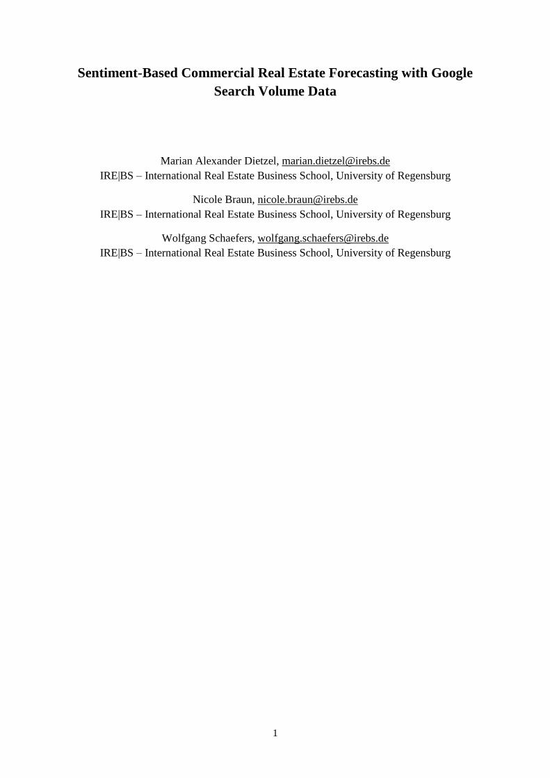
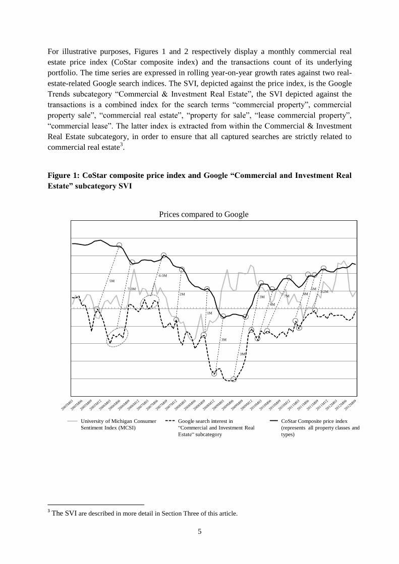
For illustrative purposes, Figures 1 and 2 respectively display a monthly commercial real
estate price index (CoStar composite index) and the transactions count of its underlying
portfolio. The time series are expressed in rolling year-on-year growth rates against two real-
estate-related Google search indices. The SVI, depicted against the price index, is the Google
Trends subcategory “Commercial & Investment Real Estate”, the SVI depicted against the
transactions is a combined index for the search terms “commercial property”, commercial
property sale”, “commercial real estate”, “property for sale”, “lease commercial property”,
“commercial lease”. The latter index is extracted from within the Commercial & Investment
Real Estate subcategory, in order to ensure that all captured searches are strictly related to
commercial real estate3.
Figure 1: CoStar composite price index and Google “Commercial and Investment Real
Estate” subcategory SVI
Prices compared to Google
University of Michigan Consumer
Sentiment Index (MCSI)
5M
7-3M
6-3M
2M
1M
3M
3M
3M
4M
7M4M
5M3-2M
-100
-80
-60
-40
-20
0
20
40
-0.25
-0.2
-0.15
-0.1
-0.05
0
0.05
0.1
0.15
0.2
0.25
g_inv_subcat co_compGoogle search interest in
“Commercial and Investment Real
Estate“ subcategory
CoStar Composite price index
(represents all property classes and
types)
3 The SVI are described in more detail in Section Three of this article.
6
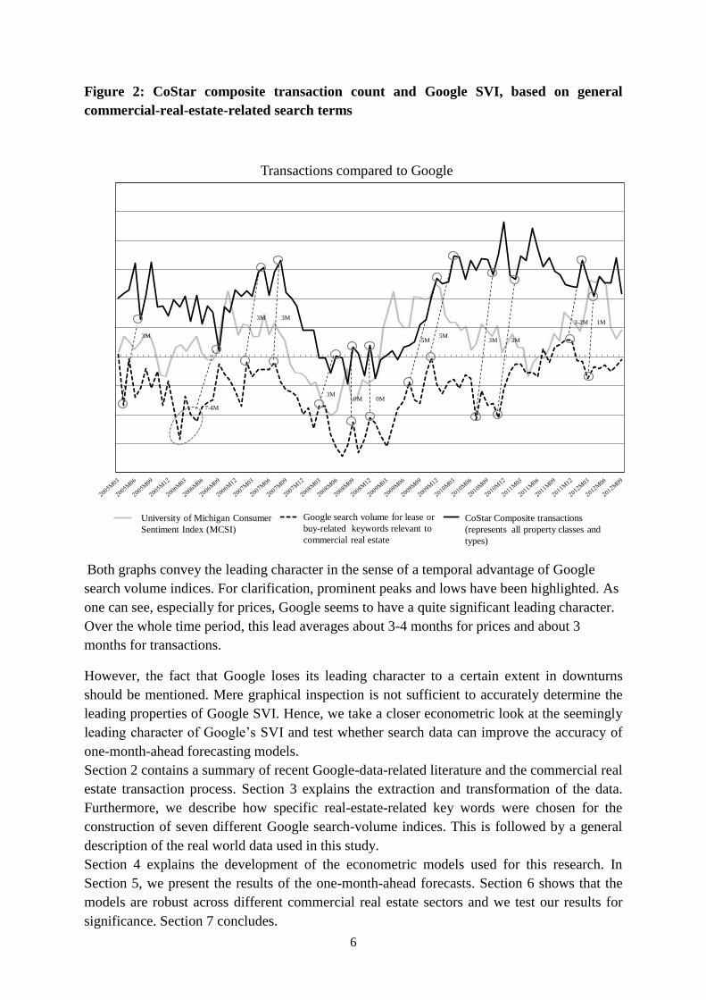
Figure 2: CoStar composite transaction count and Google SVI, based on general
commercial-real-estate-related search terms
Transactions compared to Google
-800
-600
-400
-200
0
200
400
600
-20
-15
-10
-5
0
5
10
15
20
25
30
g_comm co_comp_tra
3M
7-4M
3M3M
3M0M 0M
5M5M
3M 3M
3-2M 1M
CoStar Composite transactions
(represents all property classes and
types)
Google search volume for lease or
buy-related keywords relevant to
commercial real estate
University of Michigan Consumer
Sentiment Index (MCSI)
Both graphs convey the leading character in the sense of a temporal advantage of Google
search volume indices. For clarification, prominent peaks and lows have been highlighted. As
one can see, especially for prices, Google seems to have a quite significant leading character.
Over the whole time period, this lead averages about 3-4 months for prices and about 3
months for transactions.
However, the fact that Google loses its leading character to a certain extent in downturns
should be mentioned. Mere graphical inspection is not sufficient to accurately determine the
leading properties of Google SVI. Hence, we take a closer econometric look at the seemingly
leading character of Google’s SVI and test whether search data can improve the accuracy of
one-month-ahead forecasting models.
Section 2 contains a summary of recent Google-data-related literature and the commercial real
estate transaction process. Section 3 explains the extraction and transformation of the data.
Furthermore, we describe how specific real-estate-related key words were chosen for the
construction of seven different Google search-volume indices. This is followed by a general
description of the real world data used in this study.
Section 4 explains the development of the econometric models used for this research. In
Section 5, we present the results of the one-month-ahead forecasts. Section 6 shows that the
models are robust across different commercial real estate sectors and we test our results for
significance. Section 7 concludes.
7
2. Literature Review
2.1. Research with Google Search Volume Data
A large variety of social/economic activities now take place online. In our developed world,
everyday-life without the internet seems unimaginable for private and business consumers
alike. According to www.forrester.com, the internet penetration rate for the United States was
79% in December 20124, and for businesses the proportion is probably greater. Therefore,
Google search data can be regarded as largely representative.
Academic research on internet search activity has been around for about a decade, although
mainly in the field of computer science. With the launch of Google Trends in 2006,
researchers from various fields started recognising the potential of this very extensive dataset
made available by Google. Various factors suggest the suitability of Google data for our
purposes as outlined in the introduction. The collection of Google data is much cheaper than
traditional market sentiment measures like survey or interview-based indicators, and are
presented in real-time. This enables the forecasting of short-term trends. The first to make use
of these particular features in a scientific article were Ginsberg et al. (2009), who identify flu
hotspots by collecting searches related to symptoms across the United States. They find a high
correlation between internet searches and data from surveillance reports of “influenza-like
illness physician visits”. As mentioned above, Google data are publicly accessible just two
days after the search activity, whereas traditional influenza surveillance systems are typically
published with a 1-2 week delay. This time advantage makes SVI a very efficient indicator of
the flu virus spread and led to the development of an epidemic tracking tool called Google Flu
Trends5.
Later the same year, Google’s chief economist Hal Varian and his colleague Hyunyoung Choi
published a seminal article on how Google search data could be used for research (Choi and
Varian, 2009). By employing simple seasonal autoregressive models, they show how the
inclusion of search data reduces the mean absolute error of one-month-ahead forecasts of
retail, automotive and home sales, as well as travel to foreign countries. In an updated version
of their first article, they demonstrate similar results for the prediction of vehicles and motor
parts sales, initial claims for unemployment benefits, travel and consumer confidence (Choi
and Varian, 2012). Chamberlin (2010) replicates Choi and Varian’s research on UK data and
confirms the leading characteristics and forecasting abilities of Google search indices. He
points to the problem that the large overall rise in total searches over the last few years has led
to a falling share of specific searches, which possibly stunts the upward growth of search
indices, but reinforces downward movements. These opinions on the advantages and
disadvantages of Google data are also shared by Tierney and Pan (2012).
Askitas and Zimmermann (2009) utilise Google search data to construct an index based on
search words that job-seekers would use to find employment. Evidence shows that the index
is highly predictive of the monthly German unemployment rate.
More recently, researchers have discovered the usefulness of search data for stock markets
and investor sentiment. Dzielinski (2012) uses search data to create a novel ex ante indicator
of economic uncertainty, based on the notion that in times of uncertainty, the demand for
information increases. As a measure of uncertainty, he uses the SVI for the term “economy”.
4 http://www.forrester.com/Online+Penetration+Rate+In+The+US+Has+Stabilized+At+79/-/E-PRE4464
5 http://www.google.org/flutrends/
8
His findings suggest a negative correlation between the Google index and commonly used
measures of investor confidence. Based on an analogous concept, Preis et al. (2013) identify
98 stock-market-related search terms and find a connection between an increase in Google
search volume before stock market declines. They show that trading strategies based on these
early warning signs significantly outperform random investment strategies. Furthermore, they
conclude that national as opposed to international search volume indices explain market
movements more effectively, which is probably because the proportion of (private) traders
among internet users is higher in the U.S. than it is globally. Beer et al. (2013) construct a
Google sentiment indicator for the French market and find a correlation with commonly used
alternative sentiment indicators. Empirical tests based on a VAR-model show that investor
sentiment is predictive of short-term market returns, where a negative relationship between
investor sentiment and stock returns during the first two weeks is prevalent. Da et al. (2011)
make use of Google Trends to construct a new measure of investor attention by which they
predict trading volume. Examining search indices derived from Russell 3000 stock tickers in a
VAR-framework, they come to the conclusion that the internet-based indices lead alternative
commonly used attention measures. Moreover, they find that a rise in Google searches
predicts an increase in stock prices over the next two weeks and a reversal of the prices within
the year. Drake et al. (2012) use a SVI to measure investor demand for information. Similar to
Da et al. (2011), they obtain Google search indices for the tickers of S&P 500 stocks. Their
main findings are that investor demand increases in a period of 1-2 weeks around corporate
announcements and is positively related to media attention and news, while being negatively
associated with investor distraction6. Bank et al. (2011) use Google search data as an indicator
of stock markets activity for the German and European stock markets and find supporting
evidence that internet searches are correlated with a rise in stock trading volume and liquidity.
Wu and Brynjolfsson (2009) conducted one of the first research projects on Google data that
is solely related to real estate. They examine the influence of Google search indices on house
prices and transaction volume for 50 US states on a quarterly basis. They conclude that an
increase in the search index is positively correlated with higher transaction volumes and
prices. They find no significant connection between the “real estate” category and house
prices, which may be because of its broad and unspecified nature in terms of the searches it
captures (e.g. property management, property development). The subcategory “real estate
agencies”, on the other hand, seems robust and positively correlated with sales. By testing
forecast accuracy, they show that Google search index augmented models outperform those
without Google by a significant margin. Kulkarni et al. (2009) derive Google search indices
based on real-estate-related keywords at the city level and test their predictive power for the
Case Shiller Index for the 20 largest MSAs. By carrying out two-way regressions, they
provide evidence that Google search indices Granger-cause house prices, but not the other
way around. Also testing for causal relationships at city levels, Beracha and Wintoki (2012)
use panel vector autoregressions for 245 MSAs to demonstrate that housing-related search
data Granger-cause abnormal price movements.
Hohenstatt et al. (2011) confirm these results at a national level for the 20 largest MSAs.
Testing whether Google search data add explanatory power to housing market models, they
find that search data significantly improve the goodness-of-fit, especially where the
6 Investors conduct less internet research when distracted by more important competing earning news.
9
subcategory “Real Estate Agency” serves as a very robust indicator for transactions. In
addition, they confirm empirically the time setting for the home buying process derived from
the existing literature and the National Association of Realtors’ “Profile of Home Buyers and
Sellers 2009”. Building on their first article, Hohenstatt and Kaesbauer (2013) confirm their
results for the UK housing market. By splitting their sample into downturn and upturn phases,
they provide evidence that the relatively robust subcategory “Real Estate Agencies” works
particularly well during upswings. Also, they propose a potential stress indicator for market
soundness by filtering the “Home Financing” subcategory for mortgage approvals and find
that the transaction volume reacts much more sensitively to a change in the indicator than
house prices. McLaren and Shanbhogue (2011) also focus on UK data using SVI to construct
indicators for house prices and unemployment rates. In line with previous studies, they find
that search data help in forecasting unemployment rates and perform about equally to other
more common early indicators. The results for house prices are even more convincing, as SVI
outperform existing indicators in terms of forecasting accuracy. They also mention the
limitations of the data in that they are scaled and rehashed and that two users with different
intentions might use similar key terms to carry out their search, which may distort the index
marginally.
2.2. Investment Process
Nedleman (1999) realised early on that firms are able to improve their information
procurement and target their investment objects more precisely by making use of the internet.
Stravroski (2004) stated that the use of the internet could facilitate the access to services even
for complex products like real estate or legal services. By designing an e-business model for
commercial real estate, he shows that tenants and investors can potentially conduct an entire
real estate transaction via the internet without even leaving their desk. Of course this does not
correspond to the practice for the investment process as a whole, but it suggests that
especially during early phases of the investment decision process, internet research does play
a major role.
Henderson and Cowart (2002) show that visitors of residential and commercial real estate
brokerage websites make extensive use of the internet for their preliminary research before
making a purchase.
The body of literature of models describing the real estate investment process is large. Among
others, Pyhrr et al. (1989), , , , Baum (2009), , Farragher and Savage (2008), Farragher and
Kleiman (1996) define the decision-making/transaction process for commercial real estate.
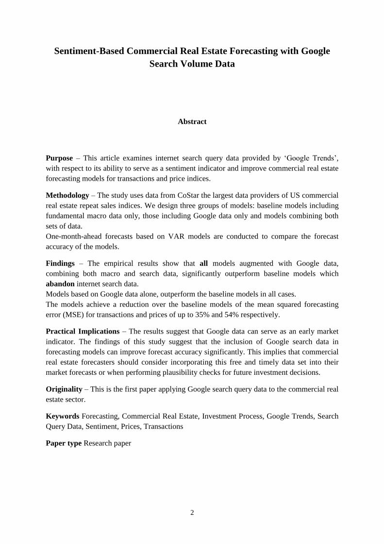
Roberts and Henneberry (2007) analyse existing literature about the normative decision-
making process to design a composite investment process combined from various models.
Based on this process, we reveal during which phases of the investment process Google
research plays a part. It seems intuitive that the moment an investor starts an internet research
is the same point in time at which he reveals his interest in real estate to Google. Figure 3
depicts the process and points out the relevant phases for internet research.
10
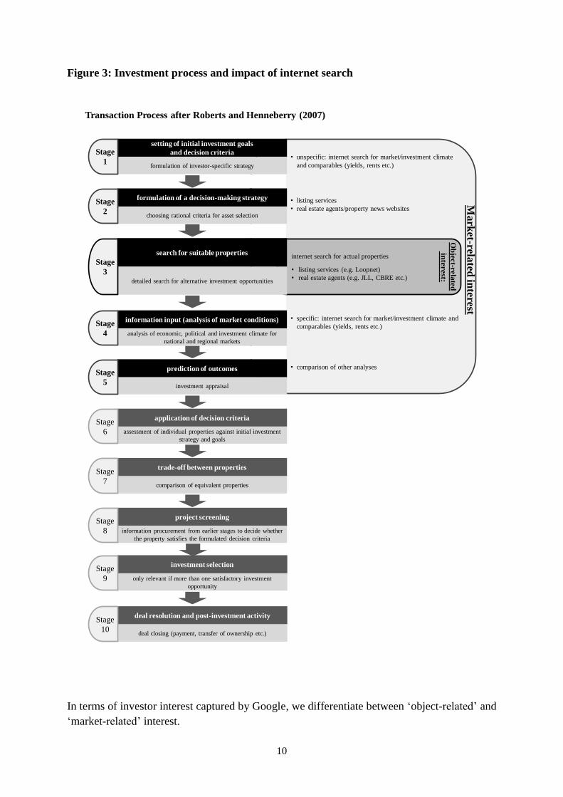
Figure 3: Investment process and impact of internet search
• unspecific: internet search for market/investment climate
and comparables (yields, rents etc.)
• listing services
• real estate agents/property news websites
• specific: internet search for market/investment climate and
comparables (yields, rents etc.)
• comparison of other analyses
Transaction Process after Roberts and Henneberry (2007)
internet search for actual properties
• listing services (e.g. Loopnet)
• real estate agents (e.g. JLL, CBRE etc.)
setting of initial investment goals
and decision criteria
formulation of investor-specific strategy
Stage
1
formulation of a decision-making strategy
choosing rational criteria for asset selection
Stage
2
search for suitable properties
detailed search for alternative investment opportunities
Stage
3
prediction of outcomes
investment appraisal
Stage
5
application of decision criteria
assessment of individual properties against initial investment
strategy and goals
Stage
6
trade-off between properties
comparison of equivalent properties
Stage
7
project screening
information procurement from earlier stages to decide whether
the property satisfies the formulated decision criteria
Stage
8
investment selection
only relevant if more than one satisfactory investment
opportunity
Stage
9
deal resolution and post-investment activity
deal closing (payment, transfer of ownership etc.)
Stage
10
information input (analysis of market conditions)
analysis of economic, political and investment climate for
national and regional markets
Stage
4
Ma
rket-rela
tedin
terest
Ob
ject-r
ela
ted
inte
rest:
In terms of investor interest captured by Google, we differentiate between ‘object-related’ and
‘market-related’ interest.
11
Object-related interest is the effort an investor makes to find a property he would like to buy.
Investors might either search for very general terms (e.g. “office property for sale”) or for
listing services/real estate agents (e.g. “Loopnet”7, “CBRE”, “JLL”) in order to access
property information online. Such interest will most probably come from investors who are
predominately interested in non-investment grade properties (e.g. private equity funds, family
offices, private investors). According to our transaction process, an investor would very likely
reveal this kind of interest during stage three.
Market-related interest is that which virtually every investor reveals during the first five
stages, and refers specifically to the analysis of market information and real estate specific
input variables (e.g. market rent, cap rate) needed for the internal investment appraisal
process. In this context investors are not interested in finding a potential investment
opportunity on the internet, but rather in gathering enough market information to make a
decision about whether or not to make a potential investment. Typically, during this phase,
research departments will look at market reports published by large real estate agents or at
commercial-property-related news websites to obtain information on rent and yield
development, the direction of movement of national and local markets and other market
activities. Furthermore, they might browse listing services or brokerage websites to find
properties comparable to the currently appraised investment opportunity, as well as potential
competition in the market.
3. Data
3.1. Data Extraction from Google Trends
Google offers search query data through its tool Google Trends 2.0, which has existed since
2012 as a merging of Google Insights and Google Trends8. Users are able to download search
volume indices that show the level of interest in certain search terms over time. These search
indices can be aggregated at international, national, state and MSA levels. Instead of absolute
numbers, the search data are normalized and scaled from 0 to 100, the latter representing the
highest search volume within the viewed time period. Thus, the trend/chart for the same
keywords can change over time, as soon as a new maximum has been reached. This has been
criticised by Tierney and Pan (2012), among others, because the aggregation of data, and the
scaling process, can lead to a loss of data.
In order to filter certain topics, Google provides categories and subcategories for specific
searches. In this respect, the search engine not only monitors a single search query at a time,
but also those a user conducts before and after. If, for example, a user had been searching for
“office” followed by “lease contract”, Google Trends would probably put this search into the
‘Real Estate’ category. If, however, he searched for “office” then “stapler”, he would most
probably be placed in the retail category.
Following the existing literature, we apply two methods to construct our search volume
indices. Similar to Askitas and Zimmermann (2009) we use popular single search terms,
combine them into one search and build an index. In addition, we make use of the
7 “LoopNet.com is the most heavily trafficked commercial real estate website, with an average of nearly four
million monthly unique visitors according to Google Analytics” Loopnet (2013) 8 https://support.google.com/trends/answer/2423202?hl=en&ref_topic=13973
12
subcategories already provided by Google Trends analogous to Choi and Varian (2012) or
Hohenstatt et al. (2011).
While subcategory indices were used as provided by Google, the following approach was
employed to construct indices based on search words.
The specific search terms were chosen by starting with logical keywords like “commercial
property” or “commercial real estate”, then adding the top “related [search] terms” suggested
by Google Trends. In order to ensure that all search interest is related to commercial real
estate only, all indices were extracted from within the “Commercial & Investment Real
Estate” subcategory provided by Google. Therefore, all single search indices form a subset of
the “Commercial & Investment Real Estate” subcategory.
Based on the above, seven different search indices were extracted from Google Trends. Each
index is based on either a different set of search keywords or a real estate subcategory.
Therefore, each index differs in its progression over time, as attempts were made to capture
various interests.
We split the seven indices into two groups, in order to generate (general) market, as well as
sector-specific search indices. While the first three indices are intended to capture general
interest in commercial real estate, the remaining four indices are aimed at finding out about
interest in specific real estate sectors (office, retail, industrial, multifamily). The latter kind
serves to show the robustness of Google Trends data in our forecasting models in section 6.
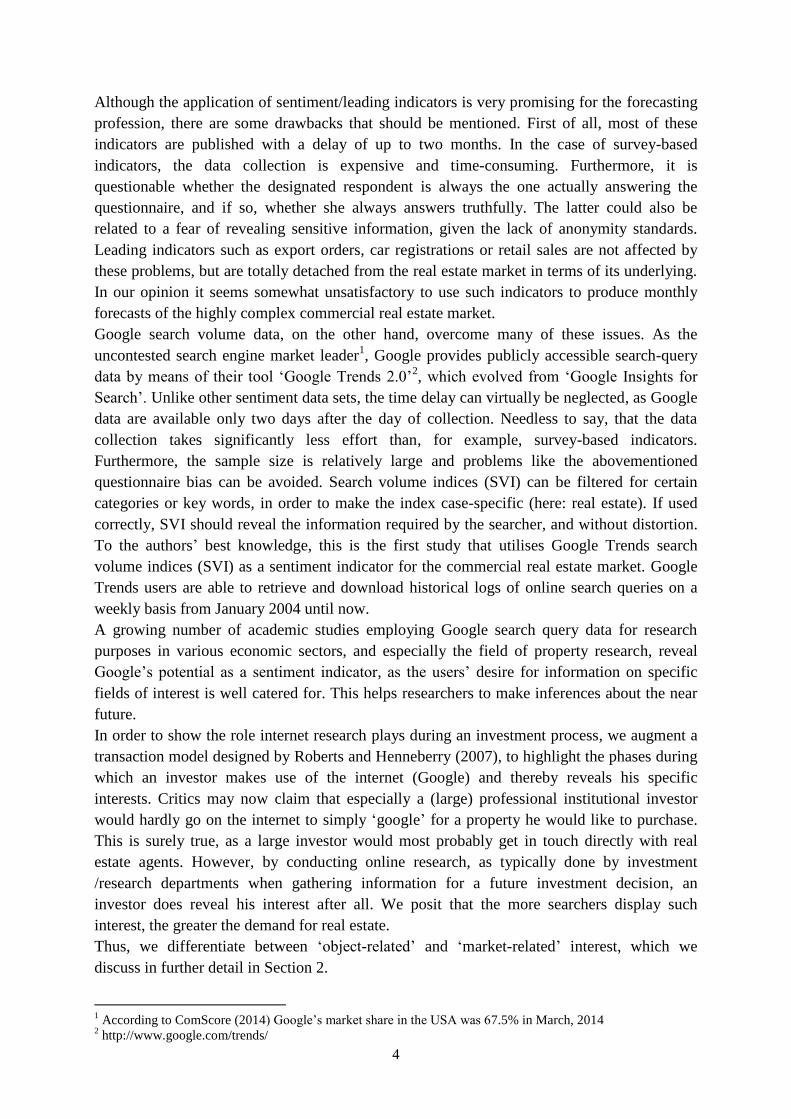
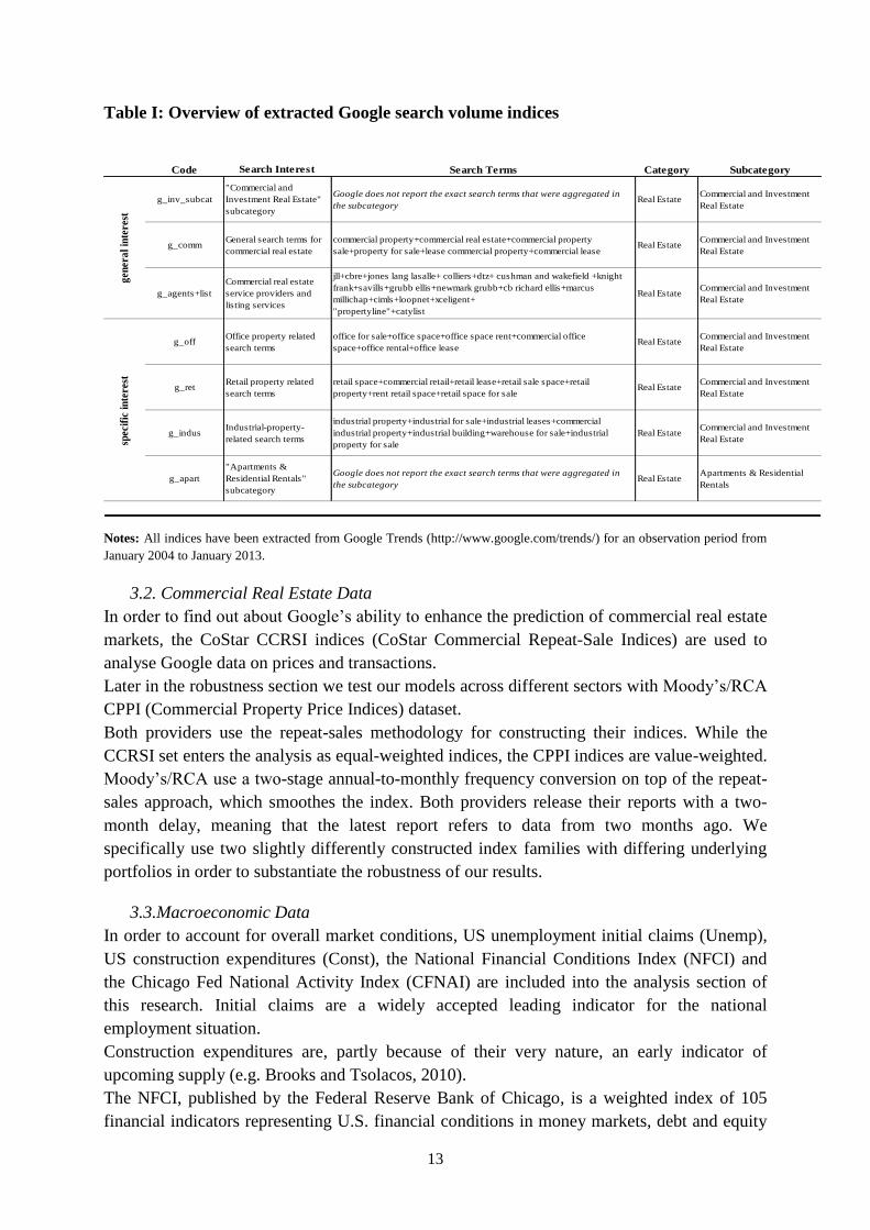
As Table I depicts, the first index is the “Commercial & Investment Real Estate” subcategory
provided by Google. The second is constructed from general search terms for commercial real
estate. The third contains search terms for large commercial real estate service providers, as
well as commercial real estate listing services such as “Jones Lang Lasalle” or “Loopnet”.
Critics might now argue that investors will not google for well-known agents. However,
googling e.g. “market report office New York” and being forwarded to a direct link to the
report is much faster and more practical than to first call up an agent’s website, look for the
research section, choose the desired property class (for example office) and finally select the
required market. If one fails to find a suitable report, then the procedure has to start from
square one, but with a different real estate service provider. Hence, searchers would very
likely first use Google to find a desired market report simply for the sake of convenience and
brevity.
Of the remaining four indices, three are linked to specific search terms related to office, retail
and industrial properties respectively. In order to capture the interest in multifamily
properties, the subcategory “Apartments & Residential Rentals” was chosen. This stems
simply from the fact that Google Trends are very unlikely to place any searches related to
apartments in the “Investment & Commercial Real Estate” subcategory.
13
Table I: Overview of extracted Google search volume indices
Code Search Interest Search Terms Category Subcategory
g_inv_subcat
"Commercial and
Investment Real Estate"
subcategory
Google does not report the exact search terms that were aggregated in
the subcategoryReal Estate
Commercial and Investment
Real Estate
g_commGeneral search terms for
commercial real estate
commercial property+commercial real estate+commercial property
sale+property for sale+lease commercial property+commercial leaseReal Estate
Commercial and Investment
Real Estate
g_agents+list
Commercial real estate
service providers and
listing services
jll+cbre+jones lang lasalle+ colliers+dtz+ cushman and wakefield +knight
frank+savills+grubb ellis+newmark grubb+cb richard ellis+marcus
millichap+cimls+loopnet+xceligent+
"propertyline"+catylist
Real EstateCommercial and Investment
Real Estate
g_offOffice property related
search terms
office for sale+office space+office space rent+commercial office
space+office rental+office leaseReal Estate
Commercial and Investment
Real Estate
g_retRetail property related
search terms
retail space+commercial retail+retail lease+retail sale space+retail
property+rent retail space+retail space for saleReal Estate
Commercial and Investment
Real Estate
g_indusIndustrial-property-
related search terms
industrial property+industrial for sale+industrial leases+commercial
industrial property+industrial building+warehouse for sale+industrial
property for sale
Real EstateCommercial and Investment
Real Estate
g_apart
"Apartments &
Residential Rentals"
subcategory
Google does not report the exact search terms that were aggregated in
the subcategoryReal Estate
Apartments & Residential
Rentals
gen
era
l in
tere
stsp
ecif
ic i
nte
rest
Notes: All indices have been extracted from Google Trends (http://www.google.com/trends/) for an observation period from
January 2004 to January 2013.
3.2. Commercial Real Estate Data
In order to find out about Google’s ability to enhance the prediction of commercial real estate
markets, the CoStar CCRSI indices (CoStar Commercial Repeat-Sale Indices) are used to
analyse Google data on prices and transactions.
Later in the robustness section we test our models across different sectors with Moody’s/RCA
CPPI (Commercial Property Price Indices) dataset.
Both providers use the repeat-sales methodology for constructing their indices. While the
CCRSI set enters the analysis as equal-weighted indices, the CPPI indices are value-weighted.
Moody’s/RCA use a two-stage annual-to-monthly frequency conversion on top of the repeat-
sales approach, which smoothes the index. Both providers release their reports with a two-
month delay, meaning that the latest report refers to data from two months ago. We
specifically use two slightly differently constructed index families with differing underlying
portfolios in order to substantiate the robustness of our results.
3.3.Macroeconomic Data
In order to account for overall market conditions, US unemployment initial claims (Unemp),
US construction expenditures (Const), the National Financial Conditions Index (NFCI) and
the Chicago Fed National Activity Index (CFNAI) are included into the analysis section of
this research. Initial claims are a widely accepted leading indicator for the national
employment situation.
Construction expenditures are, partly because of their very nature, an early indicator of
upcoming supply (e.g. Brooks and Tsolacos, 2010).
The NFCI, published by the Federal Reserve Bank of Chicago, is a weighted index of 105
financial indicators representing U.S. financial conditions in money markets, debt and equity
14
markets and banking systems. Treasury yield-, cmbs-, fixed rate mortgage- and corporate
bond yield-spreads are among the ten highest weighted subindicators 9. For this research, the
NFCI is intended to account for the general financing conditions of market participants.
The CFNAI is a weighted average of 85 economic indicators drawn from four broad
categories also published by the Federal Reserve Bank of Chicago. Among others, it includes
data on production and income, personal consumption and housing, as well as sales, orders
and inventories10
. For this study, the CFNAI is used to account for the overall US economy.
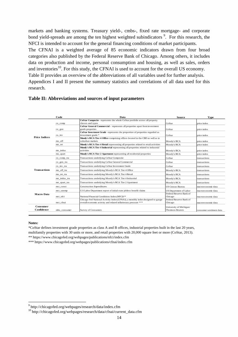
Table II provides an overview of the abbreviations of all variables used for further analysis.
Appendices I and II present the summary statistics and correlations of all data used for this
research.
Table II: Abbreviations and sources of input parameters
Code Data Source Type
co_comp
CoStar Composite - represents the whole CoStar portfolio across all property
classes and types CoStar price index
co_gen
CoStar General Commercial - represents all properties apart from investment
grade properties CoStar price index
co_inv
CoStar Investment Grade - represents the proportion of properties regarded as
investment grade * CoStar price index
mo_off
Moody's/RCA Tier 4 Office comprising offices located in the CBD as well as in
suburban markets Moody's/RCA price index
mo_ret Moody's/RCA Tier 4 Retail representing all properties related to retail activities Moody's/RCA price index
mo_indus
Moody's/RCA Tier 4 Industrial representing all properties related to industrial
activities Moody's/RCA price index
mo_apart Moody's/RCA Tier 2 Apartment representing all residential properties Moody's/RCA price index
co_comp_tra Transactions underlying CoStar Composite CoStar transactions
co_gen_tra Transactions underlying CoStar General Commercial CoStar transactions
co_inv_tra Transactions underlying CoStar Investment Grade CoStar transactions
mo_off_tra Transactions underlying Moody's/RCA Tier 4 Office Moody's/RCA transactions
mo_ret_tra Transactions underlying Moody's/RCA Tier 4 Retail Moody's/RCA transactions
mo_indus_tra Transactions underlying Moody's/RCA Tier 4 Industrial Moody's/RCA transactions
mo_apart_tra Transactions underlying Moody's/RCA Tier 2 Apartment Moody's/RCA transactions
mcr_const Construction Expenditures US Census Bureau macroeconomic data
mcr_unemp U.S Labor Department report of initial state jobless benefit claims US Department of Labor macroeconomic data
mcr_nfci National Financial Conditions Index (NFCI)**
Federal Reserve Bank of
Chicago macroeconomic data
mcr_cfnai
Chicago Fed National Activity Index (CFNAI), a monthly index designed to gauge
overall economic activity and related inflationary pressure ***
Federal Reserve Bank of
Chicago macroeconomic data
Consumer
Confidence mhu_consumer Survey of Consumers
University of Michigan/
Thomson Reuters consumer sentiment data
Price Indices
Transactions
Macro Data
Notes:
*CoStar defines investment grade properties as class A and B offices, industrial properties built in the last 20 years,
multifamily properties with 30 units or more, and retail properties with 20,000 square feet or more (CoStar, 2013).
** https://www.chicagofed.org/webpages/publications/nfci/index.cfm
*** https://www.chicagofed.org/webpages/publications/cfnai/index.cfm
9 http://chicagofed.org/webpages/research/data/index.cfm
10 http://chicagofed.org/webpages/research/data/cfnai/current_data.cfm
15
4. Analysis
4.1. Preliminary Steps
All data used for this research were retrieved as seasonally unadjusted series. In order to
account for seasonality, we put them into rolling year-on-year differences. Since Google
search data can only be downloaded on a weekly basis, they first have to be transformed into
monthly series. Weeks extending into the next month were therefore split up, weighted by
days and counted into the month to which they belong. The sample used for this study runs
from January 2004 to January 2013. Transforming the time series into year-on-year
differences implies a loss of 12 months, leaving 97 observations in total.
In order to ensure that the time series are I(0) processes, common unit root tests (Dickey and
Fuller, 1979; Phillips and Perron, 1988; Kwiatkowski et al., 1992) were employed. The tests
suggest a need for first differencing to ensure stationarity. As an additional positive effect,
first differencing resolves the issue of the downward trending of Google search indices, which
is due to the rapid increase in total search volumes over recent years and has already been
criticised, for example, by Carrière-Swallow and Labbé (2013). Due to the very volatile
nature of the year-on-year transaction counts, we put them into log form to account for
outliers.
4.2. Granger-causality
In order to study the relationship between Google SVI, real estate indices and transactions, we
perform pairwise Granger-causality tests (Granger, 1969). As a specification, we assume a
lag-order of 12 which, as a period of one year, is adequate for the analysis. Additionally, we
perform the tests with six lags to check our results for consistency.
Basic model for testing Granger-causality:
(1)
(2)
where is either 6 or 12 lags as described above; represents prices/transactions and
stands for the Google SVI.
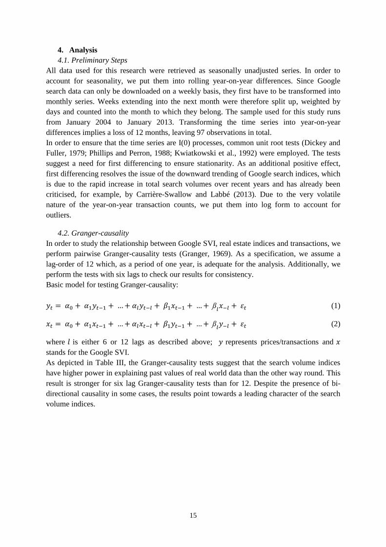
As depicted in Table III, the Granger-causality tests suggest that the search volume indices
have higher power in explaining past values of real world data than the other way round. This
result is stronger for six lag Granger-causality tests than for 12. Despite the presence of bi-
directional causality in some cases, the results point towards a leading character of the search
volume indices.
16
Table III: Granger-causality tests between prices/transactions and Google SVI
g_agents_list g_comm g_inv_subcat g_agents_list g_comm g_inv_subcat
dependent ** *** ** **/+ ** ***/++
independent **/++ */++ ***/+++ **
dependent * ** *** ***/++ */++ **/++
independent + ++ */++ **/+++ *
dependent ** ***/++ *** **/++
independent ** ++
co_gen
co_comp
co_inv
Prices Transactions
Notes: Performance of pairwise Granger-causality tests, where d and i represent the dependent and independent variable
respectively. The test is performed for 6 lags (indicated by “*”) and 12 lags (indicated by “+”). Significant at: */+ p < 0.10,
**/++ p < 0.05 and ***/+++ p < 0.01.
Generally, bi-directional relationships are present as shown in Table III.
For time series with interdependencies, Sims (1980) suggests the use of vector-autoregressive
(VAR) models to avoid endogeneity problems. As no clear one-side causal direction can be
determined, VAR-models seem appropriate for further analysis.
4.3. Lag Order
In VAR-models, variable adjustments responding to changes in another variable are often
inert, so that over a one-period horizon, only part of the overall effect of the change is
observable. Therefore, it is necessary to determine the optimal lag-structure before specifying
the models. One way of doing this is to pairwise estimate all Google and real estate variables
in VAR Models.
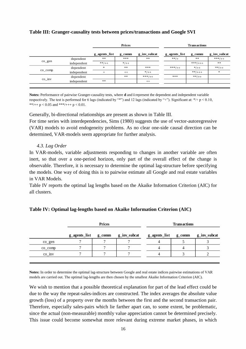
Table IV reports the optimal lag lengths based on the Akaike Information Criterion (AIC) for
all clusters.
Table IV: Optimal lag-lengths based on Akaike Information Criterion (AIC)
g_agents_list g_comm g_inv_subcat g_agents_list g_comm g_inv_subcat
co_gen 7 7 7 4 5 3
co_comp 7 7 7 4 4 3
co_inv 7 7 7 4 3 2
TransactionsPrices
Notes: In order to determine the optimal lag-structure between Google and real estate indices pairwise estimations of VAR
models are carried out. The optimal lag-lengths are then chosen by the smallest Akaike Information Criterion (AIC).
We wish to mention that a possible theoretical explanation for part of the lead effect could be
due to the way the repeat-sales-indices are constructed. The index averages the absolute value
growth (loss) of a property over the months between the first and the second transaction pair.
Therefore, especially sales-pairs which lie farther apart can, to some extent, be problematic,
since the actual (non-measurable) monthly value appreciation cannot be determined precisely.
This issue could become somewhat more relevant during extreme market phases, in which
17
vast numbers of transactions take place within a short time frame. However, even then, a
definite lead (lag) effect cannot be determined, since the first sales-pairs still differ from
transaction to transaction in terms of which cycle phase they were transacted in. Further
research could investigate this issue. There are some reasons, however, why we believe that
this problem is more theoretical than practical. Firstly, it is mitigated by a growing number of
transactions feeding into the index. CoStar provides the largest commercial real estate
database ranging back more than twenty years and including more than 1.3 million property
sale records. Consequently, many of these transactions overlap with each other in both the
past and the future. This automatically eliminates a substantial proportion of the theoretical
systematic lead/lag effect of the index. Moreover, according to CoStar most transactions
occur after a 12-month holding period, which is fairly short for commercial real estate. This
means that the value de- or appreciation of the building can be ascribed quite precisely to the
respective month for the largest part of the underlying portfolio.
We believe that at least part of the leading effect of the Google indicators stems from the fact
that they incorporate information from the early phases of the transaction process (see Section
2.2). However, not all Google research necessarily takes place during a transaction or due
diligence process, but could also be conducted at an even earlier point of time. The
commercial real estate indices on the other hand, receive their data from deal closings, which
by their very nature, occur at the end of the transaction process.
4.4.Models
We believe that at least part of the leading effect of the Google indicators stems from the fact
that they incorporate information from the early phases of the transaction process (see Section
2.2). However, not all Google research necessarily takes place during a transaction or due
diligence process, but could also be conducted at an even earlier point of time. The
commercial real estate indices on the other hand, receive their data from deal closings, which
by their very nature, occur at the end of the transaction process.
For prices, the test reveals an average of seven lags as the optimum lag length. For
transactions, a slightly shorter lag structure of four lags is, on average, suggested by the AIC.
Therefore, it can be assumed that transactions lead prices. The results are broadly in line with
the graphical analysis from Section 1 as they support the proposition that Google has a
stronger leading effect on prices than it does on transactions. From our preliminary analysis,
we find interdependencies between prices, transactions and search indices, which lead us to
use vector autoregressive (VAR) models. Based on the lag-length-tests from above, we use a
lag-order specification of six for the models.
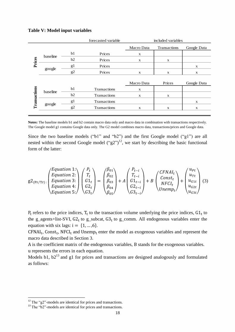
In order to test forecast accuracy, we construct four different general models, separated into
two baseline and two Google models. As a result, we obtain a total of 24 models.11
As shown
in Table V, the b1 model carries macro data and prices or transactions; b2 contains prices and
transactions as well as macro data; g1 contains prices or transactions and Google data; g2
contains all mentioned variables.
11
Twelve models for price and transaction forecasts each.
18
Table V: Model input variables
forecasted variable
Macro Data Transactions Google Data
b1 Prices x
b2 Prices x x
g1 Prices x
g2 Prices x x x
Macro Data Prices Google Data
b1 Transactions x
b2 Transactions x x
g1 Transactions x
g2 Transactions x x x
included variables
baseline
Pri
ces
Tra
nsa
ctio
ns
baseline
Notes: The baseline models b1 and b2 contain macro data only and macro data in combination with transactions respectively.
The Google model g1 contains Google data only. The G2 model combines macro data, transactions/prices and Google data.
Since the two baseline models (“b1” and “b2”) and the first Google model (“g1”) are all
nested within the second Google model (“g2”)12
, we start by describing the basic functional
form of the latter:
(3)
refers to the price indices, to the transaction volume underlying the price indices, to
the g_agents+list-SVI, to g_subcat, to g_comm. All endogenous variables enter the
equation with six lags: .
, , and enter the model as exogenous variables and represent the
macro data described in Section 3.
is the coefficient matrix of the endogenous variables, stands for the exogenous variables.
represents the errors in each equation.
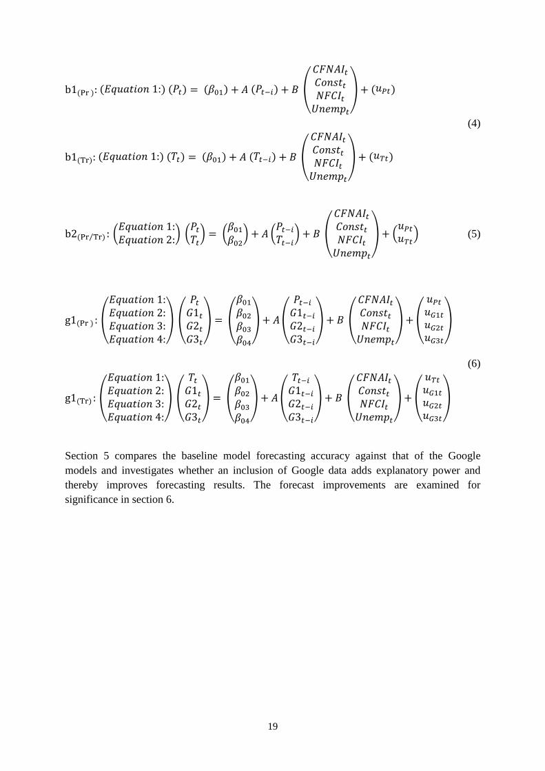
Models b1, b213
and g1 for prices and transactions are designed analogously and formulated
as follows:
12
The “g2”-models are identical for prices and transactions. 13
The “b2”-models are identical for prices and transactions.
19
(4)
(5)
(6)
Section 5 compares the baseline model forecasting accuracy against that of the Google
models and investigates whether an inclusion of Google data adds explanatory power and
thereby improves forecasting results. The forecast improvements are examined for
significance in section 6.
20
4.5. Impulse-Response-Function
Since an ordinary interpretation of VAR-models can be vague, due to various interactions
between the equations, we employ an impulse response function (IRF) to determine the
reaction of the price/transaction variables to a shock from the Google variables.
The IRF describes the reaction of the process in , when, at point of
time , a single shock hits the variable in the system (Lütkepohl et al., 2004).
In order to remain consistent, we set the observation period to six months
. The accumulated impulse response shows the total reaction over the observation period
for all possible six month-periods over the entire sample.
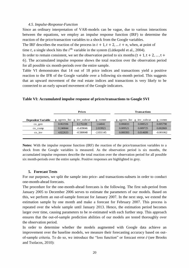
Table VI demonstrates that 14 out of 18 price indices and transactions yield a positive
reaction to the IFR of the Google variable over a following six-month period. This suggests
that an upward movement of the real estate indices and transactions is very likely to be
connected to an early upward movement of the Google indicators.
Table VI: Accumulated impulse response of prices/transactions to Google SVI
Dependent Variable g_agents_list g_inv_subcat g_comm g_agents_list g_inv_subcat g_comm
co_gen 0.061936 0.176108 1.64041 0.006833 0.008523 0.005798
co_comp 0.246844 -0.439046 2.019921 0.009521 0.009725 0.002869
co_inv 4.822633 -0.580048 -2.831145 0.000393 0.014699 -0.001062
TransactionsPrices
Notes: With the impulse response function (IRF) the reaction of the price/transaction variables to a
shock from the Google variables is measured. As the observation period is six months, the
accumulated impulse responses describe the total reaction over the observation period for all possible
six month-periods over the entire sample. Positive responses are highlighted in grey.
5. Forecast Tests
For our purposes, we split the sample into price- and transactions-subsets in order to conduct
one-month-ahead forecasts.
The procedure for the one-month-ahead forecasts is the following. The first sub-period from
January 2005 to December 2006 serves to estimate the parameters of our models. Based on
this, we perform an out-of-sample forecast for January 2007. In the next step, we extend the
estimation sample by one month and make a forecast for February 2007. This process is
repeated over the whole sample until January 2013. Hence, the estimation period becomes
larger over time, causing parameters to be re-estimated with each further step. This approach
ensures that the out-of-sample prediction abilities of our models are tested thoroughly over
the observation period.
In order to determine whether the models augmented with Google data achieve an
improvement over the baseline models, we measure their forecasting accuracy based on out-
of-sample criteria. To do so, we introduce the “loss function” or forecast error (see Brooks
and Tsolacos, 2010):
21
(7)
where are the realisations (actuals) at time and is the one-month-ahead
forecast made at time . We have 73 observations from January 2007 to January 2013.
Based on this loss function, we compute the mean squared error (MSE) for all forecasts.
(8)
Theil (1966, 1971) introduced the U1 coefficient which ranges between 0 and 1, with the
basic rule being that the closer the coefficient is to zero, the better the forecast accuracy. We
utilise the U1 coefficient in order to render the measurement of forecast accuracy of all
models comparable.
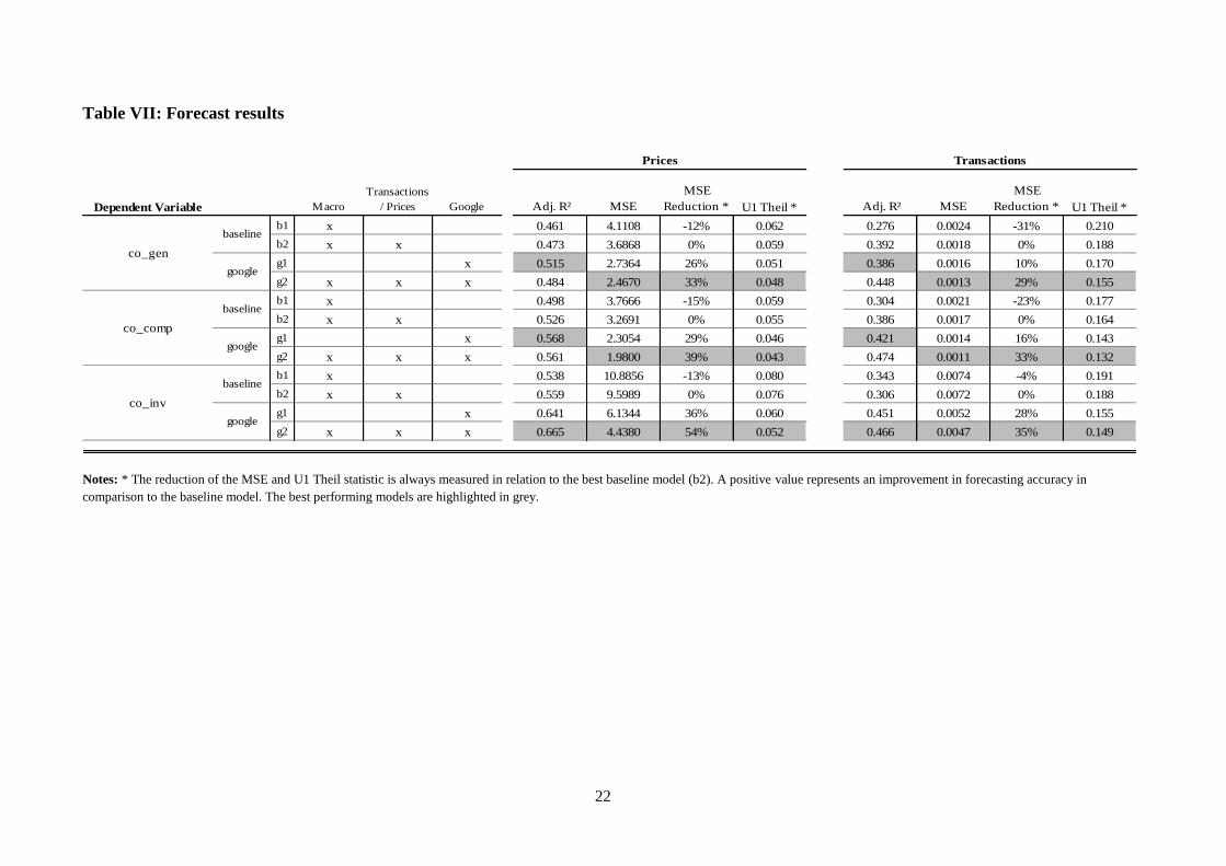
(9)We report the MSE, the MSE reduction in Google
data augmented models, against the best baseline model and Theil’s U1 statistic. In addition,
the adjusted-R² serves as a goodness-of-fit measure and in-sample criterion. Table VII gives
an overview of the results of all (24) tested models. The best performing models are
highlighted in grey.
22
Table VII: Forecast results
Dependent Variable Macro
Transactions
/ Prices Google Adj. R² MSE
MSE
Reduction * U1 Theil * Adj. R² MSE
MSE
Reduction * U1 Theil *
b1 x 0.461 4.1108 -12% 0.062 0.276 0.0024 -31% 0.210
b2 x x 0.473 3.6868 0% 0.059 0.392 0.0018 0% 0.188
g1 x 0.515 2.7364 26% 0.051 0.386 0.0016 10% 0.170
g2 x x x 0.484 2.4670 33% 0.048 0.448 0.0013 29% 0.155
b1 x 0.498 3.7666 -15% 0.059 0.304 0.0021 -23% 0.177
b2 x x 0.526 3.2691 0% 0.055 0.386 0.0017 0% 0.164
g1 x 0.568 2.3054 29% 0.046 0.421 0.0014 16% 0.143
g2 x x x 0.561 1.9800 39% 0.043 0.474 0.0011 33% 0.132
b1 x 0.538 10.8856 -13% 0.080 0.343 0.0074 -4% 0.191
b2 x x 0.559 9.5989 0% 0.076 0.306 0.0072 0% 0.188
g1 x 0.641 6.1344 36% 0.060 0.451 0.0052 28% 0.155
g2 x x x 0.665 4.4380 54% 0.052 0.466 0.0047 35% 0.149
co_inv
baseline
co_comp
baseline
co_gen
baseline
Prices Transactions
Notes: * The reduction of the MSE and U1 Theil statistic is always measured in relation to the best baseline model (b2). A positive value represents an improvement in forecasting accuracy in
comparison to the baseline model. The best performing models are highlighted in grey.
23
The strongest finding is that the g2 models have the lowest MSE and U1 statistic, and thereby
outperform the baseline models across all groups. For prices, the reduction in the MSEs
ranges between 33% and 54%, when comparing the best Google models (g2) to the best
baseline models (b2). The comparison of the b2 and g1 models indicates that models based
only on Google search indices, and the lags of the dependent variable, outperform the baseline
models every time.
For transactions, the reduction in the MSEs lies between 29% and 35%. As for prices both
Google models outperform the baseline models across all groups at all times. This provides
strong evidence that the models augmented with internet search data outperform by a large
margin the baseline models that only include fundamental market data. The results verify
existing research which is stating that the best forecasting results are achieved by combining
real world and internet data.
The in-sample criterion adjusted-R² largely supports the above findings. In all cases, the
adjusted-R² of either one of the Google models is higher than for the baseline models.
A few additional findings are worth mentioning.
Firstly, Theil’s U1 statistic suggests that price forecasts generally come closer to their actual
values than transaction forecasts. A possible explanation could be that prices are generally
less prone to large shifts, which makes them easier to predict in one-month-ahead forecasts.
The generally much lower MSE level for transactions stems from the fact that they are put
into log transformations.
Secondly, it should be mentioned that the implementation of Google data appears to work
very successfully in the prediction of investment grade property prices. This appears
somewhat puzzling at first sight. It seems intuitive, however, that larger, more expensive and
better located properties draw much more searcher attention. Hence, analogously to
residential properties, we expect the user-side interest to be well covered by Google Trends,
especially in an era in which internet presence and individually created websites play a large
role in the marketing of larger properties. Furthermore, a closer look at the MSE reveals that
the forecasting error for investment grade properties was significantly larger from the start (in
the baseline models), compared, for instance, against the ‘general’ properties index. Hence,
the clearly sharper MSE-reduction could partly stem from a mathematical background. All in
all, the results paint a clear picture. Forecasting models augmented with Google search data
are able to reduce the forecasting errors about one third.
6. Robustness
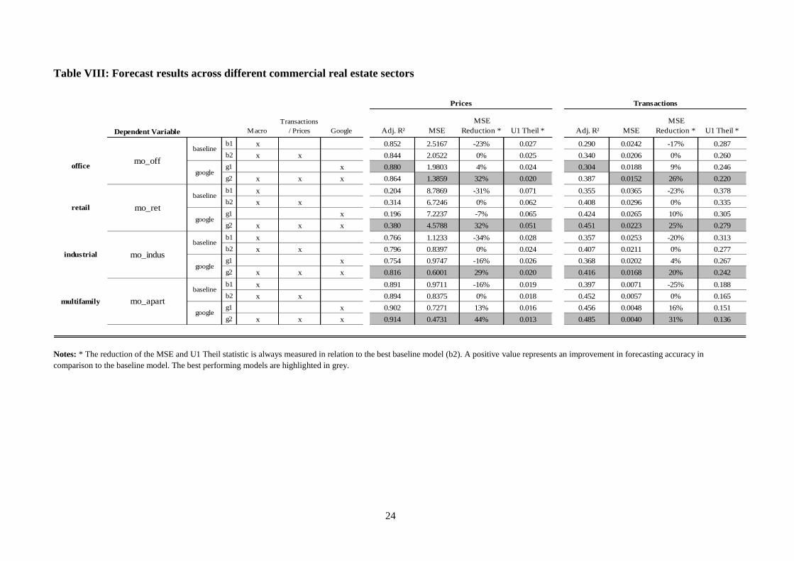
6.1. Robustness across different commercial real estate sectors
In order to test our Google data augmented forecasting models for robustness we use a
different set of commercial real estate data (RCA/Moody’s CPPI) and test them on different
sectors (office, retail, industrial, multifamily). We exchange the “G3” index g_comm by the
respective sector related search indices described in Section 3 to account for specific interest.
As illustrated in table VIII the results confirm the results from above. In all cases Google
augmented models outperform non-Google models.
24
Table VIII: Forecast results across different commercial real estate sectors
Dependent Variable Macro
Transactions
/ Prices Google Adj. R² MSE
MSE
Reduction * U1 Theil * Adj. R² MSE
MSE
Reduction * U1 Theil *
b1 x 0.852 2.5167 -23% 0.027 0.290 0.0242 -17% 0.287
b2 x x 0.844 2.0522 0% 0.025 0.340 0.0206 0% 0.260
g1 x 0.880 1.9803 4% 0.024 0.304 0.0188 9% 0.246
g2 x x x 0.864 1.3859 32% 0.020 0.387 0.0152 26% 0.220
b1 x 0.204 8.7869 -31% 0.071 0.355 0.0365 -23% 0.378
b2 x x 0.314 6.7246 0% 0.062 0.408 0.0296 0% 0.335
g1 x 0.196 7.2237 -7% 0.065 0.424 0.0265 10% 0.305
g2 x x x 0.380 4.5788 32% 0.051 0.451 0.0223 25% 0.279
b1 x 0.766 1.1233 -34% 0.028 0.357 0.0253 -20% 0.313
b2 x x 0.796 0.8397 0% 0.024 0.407 0.0211 0% 0.277
g1 x 0.754 0.9747 -16% 0.026 0.368 0.0202 4% 0.267
g2 x x x 0.816 0.6001 29% 0.020 0.416 0.0168 20% 0.242
b1 x 0.891 0.9711 -16% 0.019 0.397 0.0071 -25% 0.188
b2 x x 0.894 0.8375 0% 0.018 0.452 0.0057 0% 0.165
g1 x 0.902 0.7271 13% 0.016 0.456 0.0048 16% 0.151
g2 x x x 0.914 0.4731 44% 0.013 0.485 0.0040 31% 0.136
mo_indus
baseline
multifamily mo_apart
baseline
office
industrial
retail mo_ret
baseline
mo_off
baseline
Prices Transactions
Notes: * The reduction of the MSE and U1 Theil statistic is always measured in relation to the best baseline model (b2). A positive value represents an improvement in forecasting accuracy in
comparison to the baseline model. The best performing models are highlighted in grey.
25
The case of multifamily properties stands out to some degree. The fact that Google works
very well for residential properties seems straightforward, however, as the internet has
become one of the most important media for finding a residence. We assume that forecasting
models benefit perticularly from the well-displayed consumer demand information provided
by Google search queries. This result is in line with existing research such as Hohenstatt et al.
(2011, 2013); Wu and Brynjolfsson (2009) and Beracha and Wintoki (2012). The evidence
provided in Tables VII and VIII indicates quite clearly that the inclusion of Google Trends
data is robust in improving the in- and out-of-sample accuracy of price and transaction
forecast models for US commercial real estate markets.
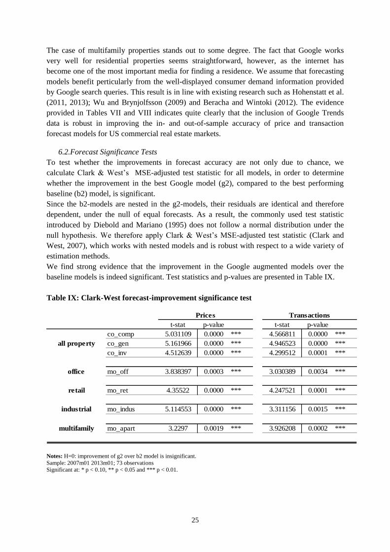
6.2.Forecast Significance Tests
To test whether the improvements in forecast accuracy are not only due to chance, we
calculate Clark & West’s MSE-adjusted test statistic for all models, in order to determine
whether the improvement in the best Google model (g2), compared to the best performing
baseline (b2) model, is significant.
Since the b2-models are nested in the g2-models, their residuals are identical and therefore
dependent, under the null of equal forecasts. As a result, the commonly used test statistic
introduced by Diebold and Mariano (1995) does not follow a normal distribution under the
null hypothesis. We therefore apply Clark & West’s MSE-adjusted test statistic (Clark and
West, 2007), which works with nested models and is robust with respect to a wide variety of
estimation methods.
We find strong evidence that the improvement in the Google augmented models over the
baseline models is indeed significant. Test statistics and p-values are presented in Table IX.
Table IX: Clark-West forecast-improvement significance test
t-stat p-value t-stat p-value
co_comp 5.031109 0.0000 *** 4.566811 0.0000 ***
co_gen 5.161966 0.0000 *** 4.946523 0.0000 ***
co_inv 4.512639 0.0000 *** 4.299512 0.0001 ***
office mo_off 3.838397 0.0003 *** 3.030389 0.0034 ***
retail mo_ret 4.35522 0.0000 *** 4.247521 0.0001 ***
industrial mo_indus 5.114553 0.0000 *** 3.311156 0.0015 ***
multifamily mo_apart 3.2297 0.0019 *** 3.926208 0.0002 ***
all property
Prices Transactions
Notes: H=0: improvement of g2 over b2 model is insignificant.
Sample: 2007m01 2013m01; 73 observations
Significant at: * p < 0.10, ** p < 0.05 and *** p < 0.01.
26
7. Conclusion
Existing research shows that internet data offer considerable potential for ‘nowcasting’ (real-
time estimation of indicators/indices that are released with a time lag) and forecasting
purposes. Google’s search volume indices are freely available and easily accessible, and
feature certain advantages over survey-based sentiment indicators, in terms of their rapid
delivery and avoidance of common interviewer effects. Combined with the fact that Google is
the unchallenged leading search engine provider with a U.S. market share of 67.5 % in March
201414
, this renders the corresponding share of searchers sufficiently representative. However,
correct and precise measurement of sentiment/interest constitutes a much greater challenge.
Especially Google’s intelligent categorisation helps researchers to capture a great chunk of
search interest for specific areas. However, particularly the absence of absolute search counts
and the way the data are scaled and rehashed, creates something of a black box in some
respects.
To the authors’ best knowledge, this is the first study examining the role of internet search
data in the commercial real estate sector. Based on a theoretical framework, we construct
various forecast models and find that the inclusion of Google data significantly improves the
one-month-ahead forecasts of commercial real estate prices and transactions for the US
market. These results are robust for the whole sample of prices and transactions supplied by
the two largest US repeat-sales index providers, whether smoothed or unsmoothed, value- or
equal-weighted, aggregated or sector-specific. In line with existing research, we come to the
conclusion that models containing both macro and Google data deliver the best forecasting
results.
The results imply that Google search data are suitable for measuring sentiment in commercial
real estate markets. Despite the fact that the commercial real estate market is dominated by
professional investors who make use of various information sources, we find that Google does
indeed often play a role during the search process before deal closing. This raises the
questions of whether this additional set of information could help to make commercial real
estate markets more efficient. Fama (1970) gives a definition of efficient market prices, which
“fully reflect” available information. Fu and Ng (2001) state that real estate markets are less
efficient than stock markets, which Clayton et al. (2009) ascribe to their highly segmented and
heterogeneous underlying assets. This causes commercial real estate markets to be inefficient
in terms of information availability. We demonstrate that Google search volume indicators
can be applied effectively to commercial real estate and thereby improve market transparency.
This allows market participants to adapt faster to changes in market climate, which could
consequently improve the market efficiency.
The apparent leading character of Google data in commercial real estate markets could make
this tool an indispensable instrument for the forecasting profession in the industry. This
corresponds to Wu and Brynjolfsson (2009), who claim that especially real estate, with its
long, research-intensive buying processes compared to stocks for example, is very suitable for
being forecasted by internet-search-data-based models. Real estate forecasters are thus
advised to make use of this dataset to improve or substantiate their forecasting results.
As a whole our findings suggest that search volume data can serve as leading indicators for
short-term trends or even turning-points in the market. In general, we believe that there is
great potential for multiple-month-ahead market forecasts, for which Google’s search index
forecasting tool could create further advantages for estimating market sentiment and as a
14
Comscore (2014)

27
consequence, market movement. This kind of information could certainly contribute to real
estate investors’ investment decisions and selection processes.
Further research should also examine Google’s explanatory power with respect to rent trends.
This includes focussing on the demand for space by the user side. If successful, price bubbles
or market turnarounds could potentially be detected at an early stage.
More generally, research in this area should be extended to MSA/city level and the specific
behaviour of Google search volume indices during downturns and upswings, and to the
performance predictability of indirect real estate investment vehicles and other financial
market products, such as REITs, CMBS or MBS.
28
References
Askitas, N. And Zimmermann K. F. (2009), “Google Econometrics and Unemployment
Forecasting”, Applied Economics Quarterly, Vol. 50 No. 2, pp. 107-20.
Bank, M., Larch, M. and Peter, G. (2011), “Google search volume and its influence on
liquidity and returns of German stocks”, Financial Markets and Portfolio Management, Vol.
25 No. 3, pp. 229-64.
Baum, A. (2009), Commercial Real Estate Investment – A Strategic Approach, 2nd
Edition,
Elsevier.
Beer, F. , Hervé, F. and Zouaoui, M. (2013), “Is Big Brother Watching Us? Google, Investor
Sentiment and the Stock Market”, Economics Bulletin, Vol. 33 No. 1, pp. 454-66.
Beracha, E. and Wintoki, J. (2012), “Predicting Future Home Price Changes Using Current
Google Search Data,” Journal of Real Estate Research, forthcoming.
Brooks, C. and Tsolacos, S. (2010), “Forecast evaluation”, Real Estate Modelling and
Forecasting, Cambridge: Cambridge University Press, pp. 268-302.
Carriére-Swallow, Y. and Labbé, F. (2013), “Nowcasting with Google Trends in an Emerging
Market”, Journal of Forecasting, Vol. 32 No. 4, pp. 289-98.
Chamberlin, G. (2010), “Googling the present”, Economic & Labour Market Review,
December 2010, pp. 59-95.
Choi, H. and Varian, H. (2009), “Predicting the Present with Google Trends”, Google
Research, Google Inc.
Choi, H. and Varian, H. (2012), “Predicting the Present with Google Trends”, Economic
Record, Vol. 88 No. s1, pp. 2-9.
Clark, T.E. and West, K.D. (2007), “Approximately normal tests for equal predictive
accuracy in nested models”, Journal of Econometrics, Vol. 138 No. 1, p. 291-311.
Clayton, J., Ling, D.C. and Naranjo, A. (2009), “Commercial Real Estate Valuation:
Fundamentals versus Investor Sentiment”, The Journal of Real Estate Finance and
Economics, Vol. 38 No. 1, pp. 5-37.
Comscore (2014), “comScore Releases March 2014 U.S. Search Engine Rankings”, available
at:
http://www.comscore.com/ger/Insights/Press_Releases/2014/4/comScore_Releases_March_2
014_U.S._Search_Engine_Rankings (accessed 16 May 2014).
Costar (2013), Commercial Repeat-Sale Indices – Methodology, available at:
http://www.costar.com/uploadedFiles/About_Costar/CCRSI/articles/pdfs/CCRSI-
Methodology.pdf (accessed 20 June 2013).
29
Da, Z., Engelberg, J. and Gao, P. (2011), “In Search of Attention”, The Journal of Finance,
Vol. 66 No. 5, pp. 1461-99.
Dickey, D. A. and Fuller, W. A. (1979), “Distribution of the Estimators for Autoregressive
Time Series With a Unit Root”, Journal of American Statistical Association, Vol. 74, pp. 427-
31.
Diebold, F. and Mariano, R. (1995), “Comparing Predictive Accuracy”, Journal of Business
and Economic Statistics, Vol. 13 No. 3, p. 253-63.
Drake, M. S., Roulstone, D. T. and Thornock, J. R. (2012), “Investor Information Demand:
Evidence from Google Searches Around Earning Announcements”, Journal of Accounting
Research, Vol. 50 No. 4, pp. 1001-40.
Dzielinski, M. (2012), “Measuring Economic Uncertainty and its Impact on the Stock
Market”, Finance Research Letters, Vol. 9 No. 3, pp. 167-75.
Fama, E. (1970), “Efficient capital markets: a review of theory and empirical work”. The
Journal of Finance, Vol. 25, No. 2, pp. 383-417.
Farragher, E.J. and Kleiman, R.T. (1996), “A re-examination of real estate investment
decisionmaking practices”, Journal of Real Estate Portfolio Management, Vol. 2 No. 1, pp.
31-39.
Farragher, E.J. and Savage, A. (2008), “An investigation of real estate investment decision-
making practices”, Journal of Real Estate Practice and Education, Vol. 11 No. 1, pp. 29-40.
Fu, Y. and Ng, L.K. (2001), “Market Efficiency and Return Statistics: Evidence from Real
Estate and Stock Markets Using a Present-Value Approach”, Real Estate Economics, Vol. 29,
No. 2, pp. 227-250.
Geltner, D. and Mei, J. (1995), “The Present Value Model with Time-Varying Discount
Rates: Implications for Commercial Property Valuation and Investment Decisions”, Journal
of Real Estate Finance and Economics, Vol. 11 No. 2, pp. 119-35.
Ghysels, E., Plazzi, A. and Valkanov, R. (2007), “Valuation in US Commercial Real Estate”,
European Financial Management, Vol. 13 No. 3, pp. 472-97.
Ginsberg, J., Mohebbi, M. H., Patel, R. S., Brammer, L., Smolinski, M. S., Brilliant, L. and
Zimmermann, K. F. (2009), “Detecting influenza epidemics using search engine query data,
Nature, Vol. 457.
Granger, C. W. J. (1969), “Investigating Causal Relations by Econometric Models and Cross-
spectral Methods”, Econometrica, Vol. 37 No. 3, pp. 424-38.
Henderson, K. V. and Cowart, L. B. (2002), “Bucking e-commerce trends: A content analysis
comparing commercial real estate brokerage and residential real estate brokerage websites”,
Journal of Corporate Real Estate, Vol. 4 No. 4, pp. 375-85.
30
Hohenstatt, R., Kaesbauer, M. and Schaefers, W. (2011), “’Geco’ and its Potential for Real
Estate Research: Evidence from the U.S. Housing Market, Journal of Real Estate Research,
Vol. 33 No. 4., pp. 471-506.
Hohenstatt, R. and Kaesbauer, M. (2013), “GECO’s Weather Forecast’ for the U.K. Housing
Market: To What Extent Can We Rely on Google ECOnometrics?”, Journal of Real Estate
Research, forthcoming.
Krystalogianni, A., Matysiak, G. and Tsolacos, S. (2004) “Forecasting UK commercial real
estate cycle phases with leading indicators: a probit approach”, Applied Economics, Vol. 36
No. 20, pp. 2347-56.
Kulkarni, R., Haynes, K. E., Stough, R. R. and Paelinck, J. H. P. (2009), “Forecasting
Housing Prices with Google Econometrics”, Research Paper School of Public Policy, George
Mason University, No. 2009-10.
Kwiatkowski, D., Phillips, P. C. B., Schmidt, P. and Shin, Y. (1992), “Testing the null
hypothesis of stationarity against the alternative of a unit root”, Journal of Econometrics, Vol.
54, pp. 159-78.
Loopnet (2013), “Quick Stats: Traffic Summary”, available at:
http://www.loopnet.com/xNet/Mainsite/Marketing/About/TrafficSummary.aspx (accessed 30
July 2013).
Lütkepohl, H. and Krätzig, M. (2004), Applied time series econometrics, Cambridge
University Press, New York.
MacKinnon, G.H. and Al Zaman, A. (2009), “Real Estate for the Long Term: The Effect of
Return Predictability on Long-Horizon Allocations”, Real Estate Economics, Vol. 37 No. 1,
pp. 117-53.
Malizia, E.E. (1991), “Forecasting Demand for Commercial Real Estate Based on the
Economic Fundamentals of U.S. Metro Markets”, Journal of Real Estate Research, Vol. 6
No. 6, pp. 251-66.
McLaren, N. and Shanbhogue, R. (2011), “Using internet search data as economic
indicators”, Quarterly Bulletin 2011 Q2, pp. 134-40.
Nedleman, A.G. (1999), “E-Commerce and Real Estate: A Phantom Menace?”, The Los
Angeles Business Journal, available at: www.securitization.net/pdf/EcommerceArticle.pdf
(accessed 27 July 2013).
Phillips, P. C. B and Perron, P. (1988), “Testing for a unit root in time series regression”,
Biomètrika, Vol. 75 No. 2, pp. 335-46.
Plazzi, A., Torous, W. and Valkanov, R. (2010), “Expected Returns and Expected Growth in
Rents of Commercial Real Estate”, The Review of Financial Studies, Vol. 23 No. 9, pp. 3469-
519.

31
Plazzi, A., Tourous, W. and Valkanov, R. (2012), “Forecasting Real Estate Prices”, in Elliot
G. and Timmermann A. (Eds.), Handbook of Economic Forecasting: Vol. 2, Elsevier,
forthcoming.
Preis, T., Moat, H.S., Stanley, E. (2013), “Quantifying Trading Behavior in Financial Markets
Using Google Trends”, Nature - Scientific Reports, Vol. 3 No. 1684, pp. 1-6.
Pyhrr, S.A., Cooper, J.R., Wofford, L.E., Kapplin, S.D. and Lapides, P.D. (1989), Real estate
investment: strategy, analysis, decisions, John Wiley and Sons, New York.
Roberts, C. and Henneberry, J. (2007), “Exploring office investment decision making in
different European contexts”, Journal of Property Investment and Finance, Vol. 25 No. 3, pp.
289-305.
Sims, C. (1980), “Macroeconomics and reality”, Econometrica, Vol. 48 No. 1, pp. 1-48.
Stravroski, B. (2004), “Designing a new e-business model for a commercial real estate
enterprise: a case study”, Online Information Review, Vol. 28 No. 2, pp. 110-119.
Theil, H. (1966), Applied Economic Forecasting, The University of Chicago Press, Chicago,
IL.
Theil, H. (1971), Principles of Econometrics, Amsterdam: North-Holland Publishing Co.
Tierney, H. L. R. and Pan, B. (2012), “A Poisson Regression Examination of the Relationship
between Website Traffic and Search Engine Queries”, Netnomics: Economic Research and
Electronic Networking, Vol. 13 No. 3, pp. 155-89.
Tsolacos, S. (2012), “The role of sentiment indicators for real estate market forecasting”,
Journal of European Real Estate Research, Vol. 5 No. 2, pp. 109-20.
Wheaton, W.C. (1987), “The Cyclic Behavior of the National Office Market”, Real Estate
Economics, Vol. 15 No. 4, pp. 281-99.
Wu, L. and Brynjolfsson, E. (2009), “The Future of Prediction: How Google Searches
Foreshadow Housing Prices and Sales”, Working papers, Wharton School, University of
Pennsylvania.