FORECASTING THE REAL ESTATE MARKET: A COINTEGRATED APPROACH

_______________

A Thesis

Presented to

The Faculty of the Department

of Economics

University of Houston

_______________

In Partial Fulfillment

Of the Requirements for the Degree of

Master of Arts

_______________

By

Jaweria Seth

August, 2011

FORECASTING THE REAL ESTATE MARKET: A COINTEGRATED APPROACH

_______________

An Abstract of a Thesis

Presented to

The Faculty of the Department

of Economics

University of Houston

_______________

In Partial Fulfillment

Of the Requirements for the Degree of

Master of Arts

_______________

By

Jaweria Seth

August, 2011

ABSTRACT

Research has shown that a decline in residential investments signals an impending

decline in economic activity. Sources of demand for both residential and commercial real

estate sectors are similar and this should move the markets in the same direction over the

long-run. Since the residential market has already collapsed, the study of real estate

investments is important. This paper utilizes real estate and macroeconomic data to

forecast investment loans. Cointegration methods are used for the forecast because the

data displays a tendency to move together. The results show that the forecast is

inconsistent with the positive relationship between both real estate markets; the

residential market will continue to decline, whereas the commercial market with see a

positive growth from 2011-2012.

iv

TABLE OF CONTENTS

1. Introduction. . . . . . . . . . . . . . . . . . . . . . . . . . . . . 1

2. Methodology. . . . . . . . . . . . . . . . . . . . . . . . . . . . . 4

2.1 Data. . . . . . . . . . . . . . . . . . . . . . . . . . . . . . . 4

2.1.1 DF-GLS Test for Unit Root. . . . . . . . . . . . . . . . . . 5

2.1.2 Structural Breaks. . . . . . . . . . . . . . . . . . . . . . 7

2.2 Modeling. . . . . . . . . . . . . . . . . . . . . . . . . . . . . 8

2.3 Forecasting. . . . . . . . . . . . . . . . . . . . . . . . . . . . 13

3. Results. . . . . . . . . . . . . . . . . . . . . . . . . . . . . . . 15

3.1 Modeling. . . . . . . . . . . . . . . . . . . . . . . . . . . . . 15

3.1.1 Residential Real Estate (RRE). . . . . . . . . . . . . . . . . 15

3.1.2 Commercial Real Estate (CRE) . . . . . . . . . . . . . . . . 16

3.2 Forecasting. . . . . . . . . . . . . . . . . . . . . . . . . . . . 19

3.2.1 Residential Real Estate (RRE). . . . . . . . . . . . . . . . . 19

3.2.2 Commercial Real Estate (CRE) . . . . . . . . . . . . . . . . 21

4. Conclusion. . . . . . . . . . . . . . . . . . . . . . . . . . . . . . 23

Appendix. . . . . . . . . . . . . . . . . . . . . . . . . . . . . . . . . . 25

References. . . . . . . . . . . . . . . . . . . . . . . . . . . . . . . . . 26

v

1

1. INTRODUCTION

Research has shown that a decline in residential investments signals an impending

decline in economic activity (Leamer, 2007). This is confirmed by the burst of the most

recent housing bubble in 2007. The financial crisis that followed forced large institutions

to fail which caused a major recession. Specifically, Leamer (2007) shows that in the year

proceeding recessions, problems in the residential investment market contributed to 26%

of the decline in the economy. Many previous studies have focused on the housing

market since it affects people on a personal level; however, the study of the commercial

market is also important because this sector is large with a high financial leverage.

Additionally, problems in housing market lead to problems in the commercial market.

This is cause for great concern given the current state of the economy. Companies that

are associated with the residential market, such as construction and retail industries, grew

quickly as well and expanded the demand for commercial real estate. As a result of the

housing bubble burst, a decline in residential investment caused greater declines in

consumer spending, decreasing the demand for commercial real estate (Feldstein, 2007).

Since the fundamental sources of demand for both real estate sectors are similar, the

markets should move in the same direction over the long-run (Gyourko, 2009).

In order to study how real estate investments will perform, this paper focuses on

forecasting commercial and residential real estate loans. Previous research has focused

on using investment returns to determine the state of the real estate market; however

loans are used since they are a more direct measure of the investment. Since the loans

series and other variables of interest display a tendency to move together in the long run,

the Johansen test for cointegration is first used to analyse whether real estate loans and

2

other real estate variables and macroeconomic variables endogenously related to loans

are cointegrated. Several model specifications are used, including variables that seem to

move together in the long run, to determine which combination of variables best models

the real estate loan market. Using information criteria, the cointegrated VAR models are

assessed to choose the optimal model, which best represents each real estate sector.

Models are assessed both with the inclusion and the exclusion of structural breaks

because different models vary in regards to their sensitivity to breaks (Timmermann,

2006). This suggests that the model, and specifically the forecast, accuracy does not

depend on the whether breaks are included in the model.

After choosing the optimal model specification, with and without breaks, for the

commercial and residential real estate sectors, a forecasting exercise for all models is

done. Rolling and recursive forecasting methods are used on the 2 best model

specifications in each sector to determine which one is more accurate in forecast ability

on average throughout the full sample. Forecast accuracy is based on minimizing the

root mean square error (RMSE). The optimal specification is then used to model both

commercial and residential real estate sectors, and to forecast the 2011-2013 period.

Though there have been several studies employing cointegration techniques to the

real estate market, much of that research has focused on finding long-run relationships

between real estate variables and financial assets1. Additionally, the real estate studies

were more concentrated on the residential market, with the exception of Chaudhry, Myer,

1 These studies find long-run cointegrating relationships between real estate variables and financial asset

variables using the Johansen method. Ullah & Zhou (2003) studied the relationship between housing sales, housing prices, the 30-year mortgage rate and the NYSE stock index returns. Tuluca, Seiler, Myer, & Webb (1998) studied the relationship between the financial assets (t-bill, bonds, and stocks) and securitized/un-securitized real estate loans. Chaudhry, Myer, & Webb (1999) studied the relationship between financial assets and commercial real estate.

3

& Webb (1999), who studied the commercial real estate market. This is also the case with

studies that looked at the connection between real estate variables and macroeconomic

variables2.

Furthermore, there have not been many studies undertaken that forecast real

estate variables using the cointegrated VAR model. Zhou (1997) forecasted residential

sales and prices using the recursive technique. However, the author used the Engle and

Granger method of cointegration. On the other hand, Tuluca, Seiler, Myer, & Webb

(1998) employed the Johansen method and performed a straightforward forecast with a

holdout period of 8 observations to forecast the returns on securitized and un-securitized

real estate as well as returns on other financial assets (including t-bill, stocks, and

bonds). However, they were interested in the relationships between different financial

assets for portfolio investment decisions, rather than the real estate assets‟ relationship to

the macroeconomy.

The lack of research on multivariate cointegrating relationships between real

estate variables (including loans) and macroeconomic variables (including interest rates,

GDP, and employment) and is due to the non-stationarity of the real estate variables.

Conventional time series analysis, such as ARMA and VARs, requires stationary

variables. The use of non-stationary variables in these procedures would be incorrect

because the standard assumptions for asymptotic analysis will not be valid (Brooks &

Tsolacos, 2010). Also, the studies that applied cointegration techniques to the real estate

sector were more interested in modeling and explaining the long-run relationships

2 Kim, Goodman, & Kozar (2006) studied the relationship between home sales/construction market and

interest rate changes. Fei, Yun, and Cheng (2010) studied the relationship between housing prices in different cities. Zhou (1997) found a cointegrating relationship between home sales and home sale prices.

4

between the variables rather than forecasting certain variables.

This paper contributes to the existing literature in two ways: First, it applies a

cointegrated VAR model to model real estate loans in both the commercial and

residential sectors. Second, this paper assesses forecast accuracy using both rolling and

recursive forecasting methods under a cointegrated VAR model. The results of this

exercise is then used to forecast commercial and residential real estate loans to predict

the evolution of the real estate market from 2011-2013.

The rest of the paper is as follows: Section 2 describes the data and methodology

used to forecast a cointegrated VAR model. Section 3 presents the results from the

cointegration analysis and the forecasts. Section 5 concludes this study.

2. METHODOLOGY

2.1 Data

The commercial and residential real estate data used in this study was acquired

from BBVA Research. National data was obtained from 1950 to 2010 in quarterly

measures. Apart from the variables that were already in percentages, variables were

transformed into their logarithmic forms to rescale the data (Brooks & Tsolacos, 2010).

Commercial real estate variables comprise of total loans in dollars (“creloans”),

investment returns (“creret”), vacancy (“crevac”) and delinquency (“credel”) rates,

consumer price index (“cpi”), gross domestic product (“gdp”), service employment

(“service”), and interest rate variables including the federal funds rate (“fed”) and the ten

year treasury bill rate (“tenyr”). Residential real estate variables comprise of total loans in

dollars (“rreloans”), total number of existing home sales (“exist”), delinquency rates

(“rredel”), house price index (“hp”), gross domestic product (“gdp”), unemployment rate

5

(“ur”), and interest rate variables including the federal funds rate (“fed”) and the 30-year

mortgage rate (“mort30y”).

These variables are tested for unit root as a preliminary step to the cointegration

method. The specific variables of interest are commercial and residential real estate loans.

This data shows an increase in both sectors‟ loans since 1950 with a decline in late

2000‟s. Figure 1 shows that possible structural breaks may occur in the data due to the

slope change in the trend function. The following section provides the method and results

of unit root testing and obtaining break points in the data.

0

2000

4000

6000

8000

10000

12000

0

200

400

600

800

1000

1200

1400

1600

1800

19

52

19

55

19

58

19

61

19

64

19

67

19

70

19

73

19

76

19

79

19

82

19

85

19

88

19

91

19

94

19

97

20

00

20

03

20

06

20

09

($ b

illio

ns)

Year

FIGURE 1: Commercial and Residential Real Estate Loans (1952-2010)

Commerical Real Estateloans "CREloans"

Residential Real Estateloans "RREloans"

2.1.1 DF-GLS Test for Unit Root:

The Dickey-Fuller General Least Squares (DF-GLS) test (1996) is used in this

study to determine the existence of unit root in the variables in level form. Commonly

used tests consist of the Augmented Dickey-Fuller (ADF) and the Phillips-Perron (PP)

tests. However, this study employs the DF-GLS test since it has been shown that the DF-

GLS test has substantially improved power when an unknown mean or trend is present

6

when compared to previous forms of the ADF test (Elliott, Rothenberg, & Stock, 1996).

Also, since Elliot, Rothenberg, and Stock have determined that the DF-GLS test works

well in small samples, this serves as an additional advantage given the dataset used in this

study.

The DF-GLS test is a modified version of the Dickey-Fuller (DF) test where the

series is detrended via a GLS regression prior to performing the DF test for unit root.

First, a GLS regression is used to estimate the intercept and trend. The regression is then

detrended using OLS regression estimators. Second, the ADF test is used on the

detrended variable by fitting the OLS regression:

∆yt = α + βyt-1 + δt + λ0∆yt-1 + λ2∆yt-2 + … + λk∆yt-k + εt, (1)

and testing the null hypothesis of unit root, H0: β= 0, against an alternative that yt is

stationary (Moody, 2009). In the above regression, k is the lag order chosen by

minimizing the modified Akaike Information Criteria (MAIC).

Ng and Perron (2001) have found that using the MAIC to determine lag length in

a DF-GLS context produces significant size and power improvements over the standard

Akaike and Schwartz-Bayesian Information Criterion (AIC and SBC). This is because the

MAIC considers the bias in the estimate of the sum of the autoregressive coefficients

when choosing the lag order (Ng & Perron, 2001). This study relies on the lag order

chosen from minimizing the MAIC when determining if variables are unit root processes.

If the DF-GLS test statistic is lower than the critical value, the null hypothesis of

unit root is rejected. According to Table 1, all of the variables are non-stationary; the null

hypothesis cannot be rejected at the 5% significance level. Therefore, it can be concluded

that all of the variables follow unit root processes.

7

TABLE 1: DF-GLS Test for Unit Root

Min MAIC P 1

RMSE 2 DF-GLS test

statistic

5% Critical

Value

Null Hypothesis

(H0=unit root)

Commercial Real Estate (CRE)

logCREloans -9.078 5 0.010 -0.936 -2.894 Fail to Reject

logservice -12.072 11 0.002 -0.145 -2.841 Fail to Reject

logcreret -8.793 7 0.011 -1.027 -2.895 Fail to Reject

logcpi -10.716 4 0.005 -1.289 -2.901 Fail to Reject

loggdp -9.391 2 0.009 -0.228 -2.915 Fail to Reject

crevac -1.750 2 0.389 -1.898 -3.027 Fail to Reject

fed 0.773 9 1.316 -2.040 -2.858 Fail to Reject

tenyr -1.072 7 0.550 -1.183 -2.890 Fail to Reject

credel -3.805 2 0.144 -0.346 -3.089 Fail to Reject

Residential Real Estate (RRE)

logRREloans -10.368 12 0.005 -1.806 -2.832 Fail to Reject

loggdp -9.391 2 0.009 -0.228 -2.915 Fail to Reject

loghp -10.228 8 0.006 -0.984 -2.875 Fail to Reject

logexist -5.705 1 0.056 -1.776 -2.959 Fail to Reject

mort30y -1.300 1 0.511 -1.309 -2.973 Fail to Reject

fed 0.773 9 1.316 -2.040 -2.858 Fail to Reject

ur -2.565 12 0.252 -2.499 -2.832 Fail to Reject

rredel -4.024 3 0.124 -1.144 -3.056 Fail to Reject

Notes: 1. P is the chosen lag length determined by minimizing the MIAC (Modified Akaike Information Criteria).

2. The RMSE corresponds to the lag length chosen by the MAIC.

Variables

2.1.2 Structural Breaks:

Testing for structural changes is an important aspect of forecasting because the

presence of breaks in the data may cause inaccurate forecasts. However, Timmermann

(2006) implies that the forecast, accuracy may not depend on the whether breaks are

included in the model since different models vary in regards to their sensitivity to breaks.

Figure 1 indicates possible slope breaks in both commercial and residential real estate

loans. The Bai (1999) likelihood ratio test is used to confirm multiple structural changes

and the location of the breaks in the data.

The Bai (1999) test is used because the model allows for lagged dependent

variables and trends in the regressors; both series that are tested for multiple breaks seem

to be trending. The testing procedure is as follows: The model is estimated under the null

hypothesis of no breaks against a single break. If the null hypothesis is rejected, the

8

model is estimated under the null of single break versus two breaks, and so on. This

procedure is repeated until the test failed to reject the null of no additional breaks

(Prodan, 2008).

Results show evidence of 3 significant breaks in both variables being tested;

commercial and residential real estate loans. The locations of the breaks are consistent

with historical events. For commercial real estate loans, the breaks occurred in 1989 Q2,

1992 Q4, and 2008 Q2. The first and second breaks correspond to the collapse and

subsequent recovery of the commercial real estate market. The third break corresponds to

the most recent financial crises, in which the real estate bubble burst after property values

peaked in 2007 (Gyourko, 2009). In regards to residential real estate loans, the breaks

occurred in 1990 Q1, 1999 Q1, and 2006 Q2. The first break occurred after the 1980‟s

housing bubble burst (Glaeser, Gyourko, & Saiz, 2008). The second and third breaks

correspond to the most recent housing bubble of 2000-2006, during which housing prices

increased sharply prior to the financial crisis (Feldstein, 2007).

2.2 Modeling

Classical regression model assumptions require that all series be stationary with

zero mean and finite variance. Since the series in this study are non-stationary, a simple

VAR model would not be valid. If non-stationary variables are present, the model may

result in a spurious regression3 (Enders, 1995). An exception to this is a model that

removes the stochastic trends and produces stationary linear relationships between

variables. Cointegration implies that certain linear combinations of the variables of the

3 Enders (1995): A spurious regression is a relationship between variables that give a high r2, and t-

statistics that seem to be significant, but in fact there does not appear to be a direct causal connection. The results have no economic meaning.

9

vector process are integrated of lower order than the process itself (Juselius, 2003).

Typically, cointegration is a linear stationary relationship between non-stationary

variables integrated to the order of 1. Variables that are cointegrated tend to move

together in the long-run. In order to test for cointegration between variables, the variables

must first be tested to determine if they are non-stationary (also known as unit root

processes).

Since the results of the DF-GLS test indicate that the variables are non-stationary,

the next step is testing for cointegration between the variables. The Johansen test is used

model the commercial and residential real estate markets since this method has the option

of choosing multiple cointegrating relationships; the number of stationary long-run

relationships between variables. Typically, as the number of variables in a model

increases, so does the number of cointegrating relationships. This test employs the use of

likelihood ratio tests to determine the number of cointegrating relationships. The number

of cointegrating relationships, the rank, is then used to estimate the cointegrated VAR

model (Juselius, 2003). In this study, the Johansen test is broken down into four steps: (1)

lag length determination and residual analysis, (2) rank test, (3) variable exclusion test,

and (4) estimating the cointegrated VAR model. The results are obtained using CATS in

RATS, version 2.

It is important to identify the optimal lag length when estimating VAR models

since results of the test can be sensitive to the number of lags (Enders, 1995). A mis-

specified model can result in a different number of cointegrating relationships. Different

information criterion, such as the AIC, SBC, and H-Q, are based on the maximum

likelihood test including a penalizing factor for the addition of extra lags (Juselius, 2003).

10

This test calculates the AIC and SBC for different values of k lags, and displays the

values that correspond to each lag. The lag lengths were chosen accordingly in each

model depending on the results of both AIC and SBC tests. If both tests give identical

results, in regards to the lag order k that minimized AIC and SBC values, lag k is chosen

to estimate the model. After the correct lag order is chosen, the VAR is modeled. All

specifications of the model are analyzed in regards to their residual autocorrelation by

evaluating the Lagrange multiplier (LM) test statistics4. When both information criteria

indicate the same lag order k, the residuals do not show significant autocorrelation.

However, when both tests give different results, the two VAR models are compared to

determine which models are white noise processes, in which the residuals cause less

autocorrelation. Typically, the smaller lag order shows significant autocorrelation in the

residuals; therefore, the higher lag order is used to estimate the model.

The most important step is determining the cointegrating rank. The rank separates

out r equilibrium errors in which the system is adjusting back towards long-run steady

state. The number of unit roots, which are the driving trends in the system, is given by p-r

where p is the number of variables in the system. The rank is chosen by using the

likelihood ratio trace test at the 5% significance level. The null hypothesis is rank=r, with

p-r unit roots in the system (Dennis, Hansen, Johansen, & Juselius, 2005). If r=0, there

are no cointegrating relationships between the variables implying that the variables do not

have any common stochastic trends and do not move together in long-run. If p>r>0, then

there is/are r relation(s) that push the system towards stationary, and if p=r, then the

system is already at its long-run steady-state (Juselius, 2003).

4 Smith (2008) found that the Lagrange multiplier (LM) test for autocorrelation performs better than the

Ljung-Box test since it has better size and power properties.

11

For small sample size models, the standard rank test‟s asymptotic distribution

does not give a good approximation to the finite sample distribution. In this case, the

Bartlett correction is relied on when determining rank. The correction takes into account

the number of parameters, lag length, rank, number of restricted deterministic terms, and

the number of unrestricted terms (Johansen, 2000). The Bartlett correction is relevant in

this study since the sample size ranges from 74 to 140 observations in quarterly

measures5. Also, it has been shown that when known structural breaks are included in a

multivariate model, new asymptotic tables are required (Johansen, Mosconi, & Nielson,

2000). In this case, the cointegration analysis involves an additional step: simulating

asymptotic trace test distributions for models that include breaks.

The rank determines the number of error correction parameters in the model, but

cannot be given economic interpretation until restrictions are placed on the cointegrating

vectors. When the number of variables in the model is large, so is the number of

cointegrating vectors. When there are multiple cointegrating vectors, it may not be

possible to identify the relationships since the number of combinations between the

variables is large (Juselius, 2003). In general, the rank describes the number of

cointegrating vectors that pull forces toward long-run steady state equilibrium; the higher

the rank, the more stable the system.

The variable exclusion test indicates which variables should be omitted in the

long-run. In certain cases, the cointegrated VAR model does not require all variables to

be present in the cointegrating relationship (Dennis et al., 2005). Models in which

5 According to Juselius (2003), a small sample size is typically 50-100 observations in quarterly measures.

12

variables that can be significantly excluded at the 5% are discarded. After the correct

model specification and rank is chosen, the cointegrated VAR model is estimated.

For a n-variable model, the (n x 1) vector xt = (x1t, x2t, …, xnt)‟ has an error-

correction representation if it can be expressed in the form:

∆xt = π0 + πxt-1 + π1∆xt-1 + π2∆xt-2 + … + πp∆xt-p + εt , (2)

where π0 = an (n x 1) vector of intercept terms with elements πi0

πi = (n x n) coefficient matrices with elements πjk(i)

π = is a matrix with elements πjk such that one or more of the πjk ≠ 0

εi = an (n x 1) vector with elements εit

(Enders, 1995)

Using the full sample, the VAR Error-Correction Model (VECM) is estimated.

The estimates of a VECM model can be interpreted as both short-run and long-run

effects. The long-run relationship measures the relations between the levels of the

variables, while the short-run dynamics measures the adjustment between the first

differences of the variables. However, the model cannot be interpreted when two or

more cointegrating vectors are present since it requires restrictions on the rank. With two

or more cointegrating vectors, there is an identification problem (Juselius, 2003).

Restrictions on the cointegrating vectors are not tested since the focus of this

paper is forecasting real estate loans, not interpreting the relationships between the

variables in the model. For each model specification, the AIC and SBC is calculated to

determine which model specification best fits the data. The optimal model is one which

minimizes both information criterions in each real estate sector, with and without their

respective structural breaks included.

13

2.3 Forecasting

Since the variables are proven to be cointegrated, forecasting is done using VAR

models with error correction terms since this method would be superior, especially in

multi-step horizons, to VAR in differences and in levels (Engle & Yoo, 1987). Clements

and Hendry (1995) showed that, in a cointegrating model, the VAR in differences

forecasted worse than the unrestricted VAR and the VAR with error corrections terms.

With small samples, the differences between an unrestricted VAR and a VAR with error

correction terms become more apparent, favouring the VAR with error correction terms.

The results also supported earlier work that as the forecast horizon increases, the

cointegrated VAR model (VECM) becomes the better choice for forecasting a

cointegrated series. Tuluca, Seiler, Myer, & Webb (1998) found that the cointegrated

VAR model forecasts are better, if not the same, compared to the VAR model forecasts6.

The full sample estimation provides four models to be used to perform the out-

of-sample forecast exercise. This forecasting exercise is done to determine which model

forecasts with the lowest root mean square forecast error (RMSE) on average in each

sector; the model that includes the breaks or the model that does not. Forecast

evaluations are carried out using two methods: rolling and recursive forecasting.

Forecasting is made difficult after a break has occurred because the new data

generating process is unknown. In this study, forecasting accuracy is compared between

the best model excluding breaks and the best model including breaks. This is done to

assess whether including structural breaks in the models will reduce forecasting errors.

6 The authors found that un-securitized real estate returns’ cointegrated VAR model forecast was superior

to the VAR model forecast. For the t-bill series, the choice between the different VAR model techniques did not make a difference in the forecasts.

14

For all models, forecasting methods that are robust to breaks are used, such as rolling

and recursive forecasting (Eklund, Kapetanios, & Price, 2009). These methods allow for

time variation and are useful in assessing a model‟s stability over time.

In a rolling window forecast, a window of size n less than the entire sample, is

modeled and forecasted. The window is then moved 4 quarters into the future and the

process is repeated. In a recursive window forecast, the window is expanded 4 quarters

into the futures at each step. Both methods are used because there exists a bias-variance

tradeoff between the two that is taken into account when deciding on which model

forecasts better on average. If there happens to be a different data generating process

throughout the series, then using the earlier data may lead to bias in the parameter

estimates and forecasts. In a recursive window scheme, the earlier data is used in all

windows and this bias can accumulate to cause higher RMSE‟s in the forecasts than

compared to models that use a smaller sample that only covers the present data

generating process. However, decreasing the sample size increases the variance of the

parameter estimates, also leading to higher RMSEs in the forecasts. This occurs in a

rolling window scheme, where the number of observations is reduced in all windows

(Clark & McCracken, 2004).

The data used in this study consists of both macroeconomic and financial series,

including GDP and investment returns, which are known to include structural breaks.

Both rolling and recursive forecasts are used because the sample size is small, so relying

only on the rolling scheme would cause an increase in parameter variance. Additionally,

since there are known structural changes in the series, relying only on the recursive

scheme will definitely cause an increase in parameter estimate bias.

15

The forecast exercise provides the optimal model for both commercial and

residential real estate sectors. The forecast for these models has the lowest RMSE on

average throughout the sample. This indicates that the model‟s forecast ability is superior

compared to others in its sector. Using the models‟ full sample estimation, the VECM is

forecasted 3-years out to predict how the economy will progress in terms of investments

in real estate.The forecast error variance decomposition analysis is performed in order to

understand short-run behavior in individual variables in response to shocks. The analysis

determines what proportion of the h-step-ahead error variance for a variable i is explained

by shocks to variable j. A shock to the i-th variable will evidently directly affect that

variable, but it will also affect all the other variables in the VAR system (Brooks &

Tsolacos, 2010).

3. RESULTS

3.1 Modeling

3.1.1 Residential Real Estate (RRE):

The restricted specification for residential real estate (RRE) loans model is

comprised of the following variables: GDP, house price index, number of existing home

sales, and the 30-year mortgage rate. These variables directly influence the demand for

RRE investment. RRE loans were modeled given different combinations of interest rate,

unemployment rate, and delinquency rate variables. Table 3.1 shows models whose

residuals are white noise processes, all parameters included are significant, and long-run

relationships are present among the variables. As shown, Model A minimizes both

information criteria from the specifications that exclude the structural breaks.

16

Alternatively, Model E minimizes both information criteria from the models that include

the breaks. The breaks are included in the model as dummy variables, such that:

sb901 = t*(T>=1990:1); sb991 = t*(T>=1999:1); and sb062 = t*(T>=2006:2).

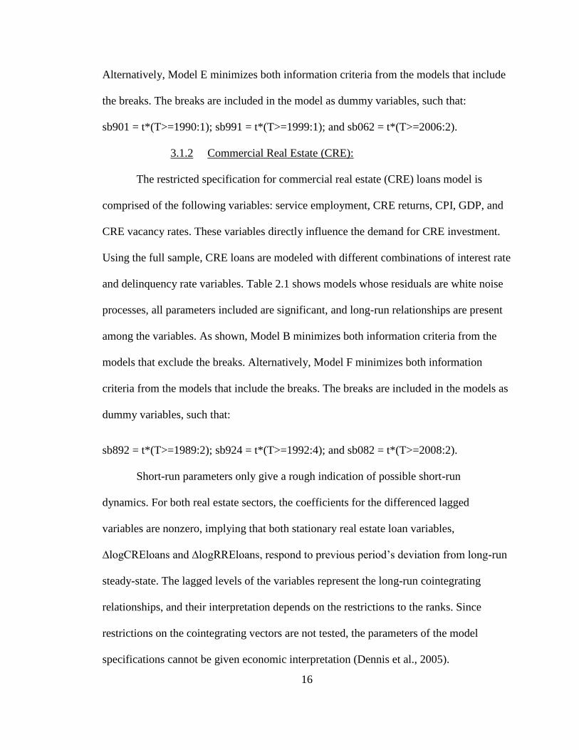
3.1.2 Commercial Real Estate (CRE):

The restricted specification for commercial real estate (CRE) loans model is

comprised of the following variables: service employment, CRE returns, CPI, GDP, and

CRE vacancy rates. These variables directly influence the demand for CRE investment.

Using the full sample, CRE loans are modeled with different combinations of interest rate

and delinquency rate variables. Table 2.1 shows models whose residuals are white noise

processes, all parameters included are significant, and long-run relationships are present

among the variables. As shown, Model B minimizes both information criteria from the

models that exclude the breaks. Alternatively, Model F minimizes both information

criteria from the models that include the breaks. The breaks are included in the models as

dummy variables, such that:

sb892 = t*(T>=1989:2); sb924 = t*(T>=1992:4); and sb082 = t*(T>=2008:2).

Short-run parameters only give a rough indication of possible short-run

dynamics. For both real estate sectors, the coefficients for the differenced lagged

variables are nonzero, implying that both stationary real estate loan variables,

∆logCREloans and ∆logRREloans, respond to previous period‟s deviation from long-run

steady-state. The lagged levels of the variables represent the long-run cointegrating

relationships, and their interpretation depends on the restrictions to the ranks. Since

restrictions on the cointegrating vectors are not tested, the parameters of the model

specifications cannot be given economic interpretation (Dennis et al., 2005).

17

TABLE 2.1: RRE Models- Full Sample Estimation

Dependent Variable: D_logRREloans

[A]* [B] [C] [D] [E]* [F] [G] [H]

Variables

Constant 0.0200 0.0027 1.6645 -0.0808 -0.3180 0.0697 1.1974 0.1045

R_Trend20.0045 0.0009 0.0039 0.0015

logRREloans{1} -0.0787 -0.0921 -0.2305 -0.1477 -0.1661 -0.0898 -0.1421 -0.1654

loggdp{1} 0.0371 0.0463 -0.1429 0.1065 0.1641 0.0554 -0.1580 0.0743

loghp{1} 0.0622 0.0692 0.1605 0.0420 0.0525 0.0422 0.1562 0.0677

logexist{1} 0.0316 0.0404 -0.0069 0.0284 0.0203 0.0204 -0.0202 0.0422

mort30y{1} -0.0011 -0.0019 -0.0034 -0.0040

fed{1} -0.0011 -0.0013 -0.0007 -0.0012

ur{1} -0.0016 -0.0001 0.0019 -0.0009

rredel{1} -0.0006 0.0009 0.0005

D_logRREloans{1} 0.1559 0.1024 0.0645 0.0432 0.1697 0.0462

D_loggdp{1} -0.1257 -0.1240 -0.1190 -0.0798 -0.1418 -0.0088

D_loghp{1} 0.0264 -0.0244 -0.0030 0.0242 0.0851 -0.0426

D_logexist{1} -0.0219 -0.0174 -0.0261 -0.0223 -0.0595 -0.0231

D_mort30y{1} -0.0034 -0.0016 -0.0004 0.0011

D_fed{1} -0.0006 -0.0003

D_ur{1} 0.0044 0.0046

D_rredel{1} 0.0026

T_1990:1 -0.0008 -0.0004 -0.0009

T_1999:1 0.0017 0.0017 0.0005 -0.0017 0.0013

T_2006:2 -0.0026 -0.0025 -0.0015 -0.0005 -0.0016

D_T_1990:1 0.0026 0.0024 0.0028

D_T_1999:1 0.0022 0.0010 0.0027 0.0046 -0.0011

D_T_2006:2 -0.0002 -0.0003 0.0002 0.0031 0.0005

Lag(s) 2 2 1 2 2 2 1 2

Rank(s) 1 1 4 3 5 5 3 5

AIC -4905 -4623 -3510 -5107 -5647 -3405 -3568 -5390

SBC -4533 -4251 -3357 -4756 -5299 -3274 -3425 -5045

Notes: 1. The specifications above are modelled in their Error-Correction form.

2. R_Trend specifies a model with linear trends in the variables and in the cointegrating relations.

* indicates the optimal model: minimizing the AIC/SBC

Models1

18

TABLE 2.2: CRE Models- Full Sample Estimation

Dependent Variable: D_logCREloans

[A] [B]* [C] [D] [E] [F]* [G] [H] [I]

Variables

Constant -0.9515 -1.0504 -1.9863 -0.9644 -0.9346 -0.2549 -1.7115 1.1465 -2.8929

R_Trend2

-0.0004 -0.0009 -0.0005 -0.0007 -0.0106

logCREloans{1} -0.1307 -0.1480 -0.1161 -0.0935 -0.1804 -0.1638 -0.1054 -0.1389 -0.0774

logservice{1} 0.0760 0.0485 0.0980 0.0418 -0.0245 -0.1356 -0.1234 -0.1577 0.1779

logcreret{1} 0.0811 0.0896 0.0592 0.0652 0.0935 0.0635 0.0106 0.1114 0.0830

logcpi{1} -0.3852 -0.3185 -0.0202 -0.0956 -0.1252 -0.3607 -0.0781 -0.3710 0.0442

loggdp{1} 0.2583 0.2799 0.1618 0.1354 0.2772 0.4784 0.6687 0.2996 0.0706

crevac{1} 0.0011 0.0016 0.0021 0.0013 0.0019 0.0013 0.0015 0.0020 0.0019

fed{1} 0.0011 0.0019 -0.0005

tenyr{1} 0.0029 0.0033

credel{1} -0.0002 -0.0015 0.0004 -0.0015 -0.0037 -0.0038

D_logCREloans{1} 0.2336 0.2126 0.2371 0.1986 0.0715

D_logservice{1} 0.4287 0.1399 -0.0549 0.0253 0.7454

D_logcreret{1} -0.2044 -0.2136 -0.1234 -0.1781 -0.0938

D_logcpi{1} 0.7198 0.5699 0.4004 0.6397 0.1896

D_loggdp{1} -0.4606 -0.4316 -0.1683 -0.5295 0.0384

D_crevac{1} -0.0055 -0.0050 -0.0053 -0.0044 -0.0043

D_fed{1} 0.0016

D_tenyr{1}

D_credel{1} 0.0007 -0.0021

T_1989:2 -0.0021

T_1992:4 0.0012 0.0052 -0.0004 -0.0022

T_2008:2 -0.0018 0.0019 0.0011 0.0037

D_T_1989:2 -0.0037

D_T_1992:4 -0.0063 -0.0055 -0.0053 -0.0157

D_T_2008:2 0.0057 0.0155 0.0232 0.0120

Lag(s) 2 2 1 1 2 2 1 1 2

Rank(s) 2 4 6 5 6 4 6 6 3

AIC -5489 -5799 -4647 -4603 -4529 -5643 -4803 -4707 -4529

SBC -5256 -5573 -4496 -4452 -4395 -5425 -4661 -4563 -4402

Notes: 1. The specifications above are modelled in their Error-Correction form.

2. R_Trend specifies a model with linear trends in the variables and in the cointegrating relations.

* indicates the optimal model: minimizing the AIC/SBC

Models1

19

3.2

3.3 Forecasting

3.3.1 Residential Real Estate (RRE):

Table 3.2 displays the results of the forecasting exercise for the RRE market. The

findings indicate that the model excluding structural breaks forecasts with a lower RMSE

on average than the model that includes the breaks. Furthermore, Model A also appears to

forecast better both in the short run and the long run. As shown in the table below, Model

A‟s forecast is superior to Model E since RMSE is minimized both at the 1-step-ahead

and 4-step-ahead forecast7.

TABLE 3.1: RRE In-Sample Forecast Exercise

Rolling

Forecast

Recursive

Forecast

Rolling

Forecast

Recursive

Forecast

1-step-ahead 0.0050 0.0041 * 0.0048 0.0062

2-steps-ahead 0.0073 * 0.0078 0.0088 0.0109

3-steps-ahead 0.0111 * 0.0133 0.0146 0.0167

4-steps-ahead 0.0176 * 0.0200 0.0205 0.0229

Notes: The Root Mean Square Errors (RMSEs) are used to assess forecast accuracy

* indicates the best model (minimizing the RMSE) for each step-ahead forecast

Model A (excluding SB) Model E (including SB)

The forecasting exercise determines that the model which excludes the structural

breaks forecasts with a minimum RMSE on average throughout the full sample. This

model is then forecasted out 3 years 2011-2013. Figure 2 suggests that residential real

estate loans will slightly decrease with a growth rate of -2.51% per year. This is a

7 Results shown in Table 3.2 also include 2- and 3-steps-ahead forecast errors. The findings are consistent

with the conclusion that model 3 forecasts with a lower RMSE on average than model 4.

20

negative outlook given that RRE loans had been declining with a rate of 2.117% per year

from its peak in 2008:1 to 2010:4.

0

2000

4000

6000

8000

10000

120001

97

6

19

79

19

82

19

85

19

88

19

91

19

94

19

97

20

00

20

03

20

06

20

09

20

12

RR

E lo

ans

($ b

illio

ns)

Year

FIGURE 2: Residential Real Estate Loans- FORECAST

Residential Real Estate loans"RREloans"

RREloans FORECAST *

The forecast error variance decomposition analysis indicates what proportion of

the 15-steps-ahead forecast error variance of variable i is explained by shocks to variable

j. It is typical for a variable to explain the majority of its forecast error variance in the

short-run and smaller fractions in the long-run. The proportion of error variance of

„logRREloans‟ that is explained by its own shocks at 4-steps-ahead is 68.61, and at 12-

steps ahead is 17.54. The proportion that is explained by shocks to „loghp‟ at 4-steps-

ahead is 16.27, and at 12-steps-ahead is 52.81. The proportion that is explained by shocks

to „mort30y‟ at 4-steps-ahead is 10.07, and at 12-steps-ahead is 16.298. This analysis

shows that shocks to the house price index will affect RRE loans in the short-run, but

they will have even more of an impact in the long-run. This can be seen in the recent

8 The proportion of error variance of ‘logRREloans’ that is explained by shocks to the remaining variables

is less than 10.00; the shocks to other variables are not going to considerable affect RRE loans in the short-run or the long-run. The Appendix shows the decomposition of variance for the series from steps 1 to 15.

21

housing bubble as evidenced by the sudden increase in house prices that led to a rapid

increase in RRE loans over the past decade.

3.3.2 Commercial Real Estate (CRE):

Table 2.2 displays the results of the forecasting exercise for the CRE market. The

findings indicate that the model including structural breaks forecasts with a lower RMSE

on average than the model that excludes the breaks. Furthermore, Model F also appears to

forecast better both in the short run and the long run. As shown in the table below, Model

F‟s forecast is superior to Model B since RMSE is minimized both at the 1-step-ahead

and 4-step-ahead forecast9.

TABLE 3.2: CRE In-Sample Forecast Exercise

Rolling

Forecast

Recursive

Forecast

Rolling

Forecast

Recursive

Forecast

1-step-ahead 0.0101 0.0100 0.0086 * 0.0099

2-steps-ahead 0.0157 0.0140 0.0134 0.0132 *

3-steps-ahead 0.0258 0.0257 0.0226 0.0222 *

4-steps-ahead 0.0317 0.0349 0.0277 0.0267 *

Notes: The Root Mean Square Errors (RMSEs) are used to assess forecast accuracy

* indicates the best model (minimizing the RMSE) for each step-ahead forecast

Model B (excluding SB) Model F (including SB)

The forecasting exercise determines that the model which includes the structural

breaks forecasts with a minimum RMSE on average throughout the full sample. This

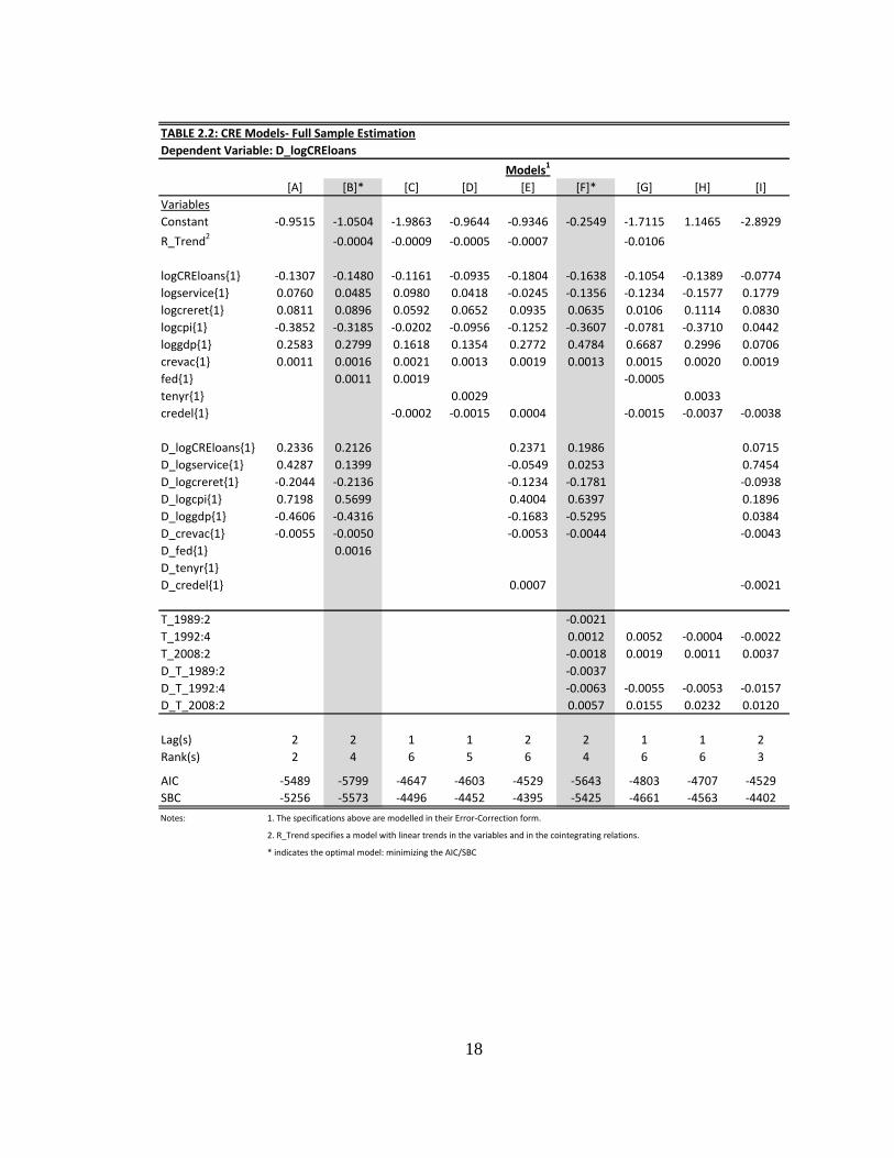
model is then forecasted out from 2011-2013. Figure 3 suggests that commercial real

estate loans will slightly increase with a growth rate of 1.99% per year. This is a positive

outlook given that CRE loans have been declining at a rate of 5.290% per year from its

9 Results shown in Table 2.2 also include 2- and 3-steps-ahead forecast errors. The findings are consistent

with the conclusion that model 2 forecasts with a lower RMSE on average than model 1.

22

peak in 2009:1 to 2010:4. However, this forecast is inconsistent with the view that CRE

and RRE loans move together. Since both sectors are driven by common fundamentals,

such as similar demand cycles, these markets should display a tendency to move together

in the long-run. A possible reason that the markets are moving in opposite directions is

the financial assistance program for banks and bank holding companies, Troubled Asset

Relief Program (TARP), that expired October 2010 (February Oversight Report, 2010).

The problems in the CRE sector and its impact on the economy, such as rising loan

default rates and declines in CRE investments, will be felt over the next few years. Since

the data in this study ends in 2010:4 and the expiration of the program is quite recent, its

effect on the CRE sector is not detected in this analysis.

0

200

400

600

800

1000

1200

1400

1600

1800

19

85

19

88

19

91

19

94

19

97

20

00

20

03

20

06

20

09

20

12

CR

E lo

ans

($ b

illio

ns)

Year

FIGURE 3: Commercial Real Estate Loans- FORECAST

Commercial Real Estate loans"CREloans"

CREloans (SB) FORECAST *

The forecast error variance decomposition analysis indicates that the proportion of

error variance of „logCREloans‟ that is explained by its own shocks at 4-steps-ahead is

69.76, and at 12-steps ahead is 16.65. The proportion that is explained by shocks to

„logservice‟ at 4-steps-ahead is 11.03, and at 12-steps-ahead is 24.97. The proportion that

is explained by shocks to „loggdp‟ at 4-steps-ahead is 12.68, and at 12-steps-ahead is

23

42.2910

. This analysis shows that shocks to service employment and gdp are going to

affect CRE loans in the short-run, but they will even more of an impact in the long-run.

4. CONCLUSION

The purpose of this study is to forecast commercial and residential real estate

loans. Since these series are non-stationary and seem to move together in the long-run,

the Johansen test is implemented to develop cointegrated VAR models for both real

estate sectors (commercial and residential). This method analyses whether real estate

loans and other endogenous real estate and macroeconomic variables, such as investment

returns, interest rates, and employment, display a tendency to move together in the long

run. Once the models are specified, with the inclusion and exclusion of structural breaks,

the Akaike and Schwartz-Bayesian information criteria statistics are minimized to decide

which model is superior in each sub-category. Out-of-sample forecasting exercise, which

includes rolling and recursive schemes, is then carried out for the 4 models that remain

to determine whether including the structural breaks in the models improves forecasting

accuracy on average throughout the sample. Results show that including the structural

breaks in the commercial real estate sector model improves forecast accuracy for both

forecasting methods. On the contrary, excluding the structural breaks in the best

residential real estate model improves forecast accuracy for both forecasting methods.

The final forecasting results obtained for both commercial and residential real estate

loans leads to the conclusion that both real estate sectors will move in opposite

directions from 2011-2013; forecasts suggest that CRE loans will increase, but RRE

10

The proportion of error variance of ‘logCREloans’ that is explained by shocks to the remaining variables is less than 10.00; the shocks to other variables are not going to considerable affect CRE loans in the short-run or the long-run. The Appendix shows the decomposition of variance for the series from steps 1 to 15.

24

loans will decrease.

Areas of further research could extend into improvements in model specifications

and forecast accuracy. To specify models that best describe the real estate loan market,

certain variables may not be strictly endogenous. A weakly exogenous variable is one

that does not adjust to the disequilibrium error. In this case, that variable could be

included in the cointegrated VAR model as an exogenous variable; set as an independent

variable with no lag parameters included. Additionally, improved methods of forecasting

could be used to minimize forecast error. Pesaran & Pick (2008) found that in the

presence of structural breaks, rolling window averaging from model could result in

lower mean square forecast errors; this is supported by empirical evidence11

.

11

Bhattacharya & Thomakos (2011) found that rolling window averaging outperformed the best window forecasts for exchange rates, inflation, and output growth more than 50% of the time across all rolling windows.

25

APPENDIX: Variance Decomposition Analysis

Step Std Error logCREloans logservice logcreret logcpi loggdp crevac

1 0.007 100.000 0.000 0.000 0.000 0.000 0.000

2 0.010 95.872 1.497 0.000 2.614 0.004 0.013

3 0.012 86.056 5.583 1.582 2.563 3.927 0.289

4 0.014 69.757 11.025 3.801 1.806 12.682 0.929

5 0.017 54.262 15.765 5.537 1.332 21.327 1.779

6 0.019 42.448 19.134 6.772 1.028 27.930 2.687

7 0.022 34.025 21.339 7.623 0.807 32.630 3.576

8 0.025 28.080 22.748 8.165 0.648 35.944 4.415

9 0.027 23.834 23.658 8.462 0.539 38.308 5.199

10 0.029 20.736 24.261 8.571 0.470 40.031 5.931

11 0.031 18.420 24.674 8.540 0.431 41.315 6.620

12 0.033 16.645 24.970 8.408 0.411 42.293 7.273

13 0.035 15.254 25.191 8.206 0.401 43.052 7.897

14 0.036 14.138 25.363 7.958 0.395 43.649 8.497

15 0.038 13.225 25.501 7.683 0.390 44.122 9.079

Step Std Error logRREloans loggdp loghp logexist mort30y

1 0.006 100.000 0.000 0.000 0.000 0.000

2 0.009 93.578 0.450 1.696 0.030 4.246

3 0.012 82.926 0.799 7.837 1.479 6.959

4 0.016 68.612 1.047 16.274 3.997 10.070

5 0.020 55.048 1.277 24.630 6.426 12.620

6 0.026 44.192 1.480 31.742 8.258 14.328

7 0.032 36.054 1.646 37.451 9.494 15.356

8 0.038 30.042 1.774 41.973 10.284 15.927

9 0.046 25.568 1.872 45.573 10.774 16.213

10 0.053 22.186 1.945 48.475 11.066 16.328

11 0.061 19.580 2.000 50.847 11.232 16.341

12 0.070 17.536 2.042 52.812 11.316 16.294

13 0.079 15.903 2.075 54.462 11.346 16.214

14 0.088 14.579 2.100 55.864 11.343 16.115

15 0.097 13.490 2.119 57.066 11.318 16.008

Decomposition of Variance for Series LOGCRELOANS

Decomposition of Variance for Series LOGRRELOANS

26

REFERENCES

Bai, J. (1999). Likelihood ratio tests for multiple structural changes. Journal of

Econometrics, 91, 299-323.

Bhattacharya, P.S. & Thomakos, D.D. (2011). Improving forecasting performance by

window and model averaging. Deakin University. Economic Series.

Brooks, C. & Tsolacos, S. (2010). Real estate modeling and forecasting. New York:

Cambridge University Press.

Chaudhry, M.K., Myer, F.C.N., & Webb, J.R. (1999). Stationarity and cointegration in

systems with real estate and financial assets. Journal of Real Estate Finance and

Economics, 18, 3, 339-349.

Clark, T.E. & McCracken, M.W. (2004). Forecast accuracy and the choice of

observation window.

Clements, M.P. & Hendry, D.F. (1995). Forecasting in cointegrated systems. Journal of

Applied Econometrics, 10, 2, 127-146.

Dennis, J.G., Hansen, H., Johansen, S., & Juselius, K. (2005). CATS in RATS: Version 2.

Illinois, USA: Estima.

Eklund, J., Kapetanios, G., & Price, S. (2009). Forecasting in presence of recent and

recurring and structural change. Bank of England.

Elliott, G., Rothenberg, T.J., & Stock, J.H. (1996). Tests for an autoregressive unit root.

Econometrica, 64, 4, 813-836.

Enders, W. (1995). Applied Econometric Time Series. USA: John Wiley & Sons, Inc.

Engle, R.F. & Yoo, B.S. (1987). Forecasting and testing in co-integrated systems.

27

Journal of Econometrics, 35, 143-159.

February Oversight Report. (2010). Commercial Real Estate Losses and the Risk to

Financial Stability. Congressional Oversight Panel.

Fei-Xue, H., Yun, Z., & Cheng, Li. (2010). Ripple effect of housing prices fluctuations

among nine cities of China. Management Science and Engineering, 4, 3, 41-54.

Feldstein, M.S. (2007). Housing, credit markets and the business cycle. National Bureau

of Economic Research, Working Paper 13471. Retrieved from

http://www.nber.org/papers/w13471

Glaeser, E.L., Gyourko, J., & Saiz A. (2008). Housing supply and housing bubbles.

National Bureau of Economic Research, Working Paper 14193. Retrieved from

http://www.nber.org/papers/w14193

Gyourko, J. (2009). Understanding commercial real estate: Just how different from

housing is it?. National Bureau of Economic Research, Working Paper 14708.

Retrieved from http://www.nber.org/papers/w14708

Johansen, S. (2000). A bartlett correction factor for tests on the cointegrating relations.

Econometric Theory, 16, 5, 740-778.

Johansen, S., Mosconi, R., Nielsen, B. (2000). Cointegration analysis in the presence of

structural breaks in the deterministic trend. Econometrics Journal, 3, 216-249.

Juselius, K. (2003). The cointegrated VAR model: Econometric methodology and

macroeconomic applications. Oxford University Press.

Kim, D.K., Goodman, K.A., & Kozar, L.M. (2006). Monetary policy and housing

market: Cointegration approach. Journal of Economics and Economic Education

Research, 7, 1, 43-52.

28

Leamer, E.E. (2007). Housing is the business cycle. National Bureau of Economic

Research, Working Paper 13428. Retrieved from

http://www.nber.org/papers/w13428

Moody, C. (2009). Basic econometrics with STATA. Economics Department. College of

William and Mary.

Ng, S. & Perron, P. (2001). Lag length selection and the construction of unit root tests

with good size and power. Econometrica, 69, 6. 1519-1554.

Prodan R. (2008). Potential Pitfalls in Determining Multiple Structural Changes With an

Application to Purchasing Power Parity. Journal of Business and Economic

Statistics, 26, 1, 50-65.

Pesaran, M.H. & Pick, A. (2008). Forecasting random walks under drift instability.

University of Cambridge. Cambridge Working Papers in Economics, 0814.

Smith, D.R. (2008). Evaluating specification tests for markov-switching time-series

models. Journal of Time Series Analysis, 29, 4, 629-652.

Timmermann, Allan. (2006) “Forecast Combinations.” In Handbook of Economic

Forecasting, edited by Graham Elliot, C.W.J. Granger, and Allan Timmermann.

Elsevier.

Tuluca, S.A., Seiler, M.J., Myer, F.C.N., & Webb, J.R. (1998). Cointegration in return

series and its effect on short-term prediction. Managerial Finance, 24, 8, 48-63.

Ullah, A. & Zhou, S.G. (2003). Real estate and stock returns: A multivariate VAREC

model. Property Management, 21, 1, 8-24.

Zhou, Z. (1997). Forecasting sales and price for existing single-family homes: A VAR

model with error correction. The Journal of Real Estate Research, 14, 155-167.