DISS. ETH No. 18120

SENSOR MODELING AND VALIDATION FOR LINEAR ARRAY AERIAL AND SATELLITE IMAGERY

A dissertation submitted to

ETH ZURICH

for the degree of

Doctor of Sciences

Presented by

SULTAN AKSAKAL - KOCAMAN

M. Sc., Middle East Technical University, Turkey

26.11.1976

citizen of Turkey

accepted on the recommendation of

Prof. Dr. Armin Gruen

Prof. Dr. Christian Heipke

2008

Dissertation Title:

Sensor Modeling and Validation for Linear Array Aerial

and Satellite Imagery

CONTENTS

Contents ……………………………………………………………………………..…. iii

Abstract ……………………………………………………………………………….... ix

Riassunto ………...……………………………………………………………………... xi

1 Introduction ………………………………………………………………............ 1

1.1 Research Objectives ……………………………………………………….… 3

1.2 Review of Digital Optical Sensors …………………………………………… 4

1.2.1 Point-based Sensors ………………………………………………. 4

1.2.2 Linear Array CCD Sensors ……………………………….……..… 4

1.2.3 Frame Array CCD Sensors …………….…..…..………….…….… 5

1.3 Review of Sensor Calibration Approaches for Linear Array CCD Sensors … 6

1.4 Review of Sensor Orientation Methods for Linear Array CCD Sensors ……. 7

1.4.1 Direct vs. Indirect Georeferencing ……………………………...….. 7

1.4.2 Rigorous vs. Generic Models for Georeferencing …………...…… 10

1.4.2.1 Generic Models for Sensor Orientation …….……………..….. 10

1.4.2.2 Rigorous Sensor Orientation of Linear Array CCD Sensors .… 11

1.4.2.2.1 Review of Trajectory Modeling Approaches ………..… 12

1.4.2.2.2 Geometric Accuracy of Aerial Linear Array CCD Sensors 13

1.4.2.2.3 Geometric Accuracy of High-resolution Satellite Optical …...

Sensors ………………………………………………… 14

iv

1.5 Quality Analysis and Validation for the Geometric Processing Methods …… 16

1.6 Outline …………………………………………….………………………… 17

2 Characterizations of the Linear Array CCD Sensor Geometries …………… 19

2.1 Optical System Specification ………………………………..…………...…. 19

2.2 Line Geometry ……………………………………………………………..... 21

2.3 Resolution Specification …………………………………………………….. 23

2.3.1 Spatial Resolution ………………………………………………..... 23

2.3.2 Radiometric Resolution …………………………………………… 24

2.3.3 Spectral Resolution ………………………………………………... 24

2.3.4 Temporal Resolutions of Satellite Sensors ……….……….………. 25

2.4 Operation Principles ……………………………………………….….…….. 25

2.4.1 Sensor and Platform Synchronization ………………….…...…….. 25

2.4.2 Stereo Acquisition ……………………………………….….…….. 27

2.4.3 Platform Stabilization …………………………………….….……. 27

3 Calibration Parameters for the Linear Array CCD Sensors ………….….….. 29

3.1 Optical System Related Parameters ……………………………….….……… 29

3.1.1 Principal Point Displacement ……...…………………….….…….. 30

3.1.2 Camera Constant ……………………………………….….……… 30

3.1.3 Lens Distortions …………………………………………….…….. 30

3.2 CCD Line Related Parameters ………………………………….…………... 32

3.2.1 Scale effect ……...………………………………….…….……….. 32

3.2.2 Rotation …………………………………………….…….……….. 32

3.2.3 Displacement from the Principal Point ………………...…………. 34

3.2.4 Bending …………………………….…………….…………….…. 34

4 Methodology for Sensor Orientation and Calibration .……………....………. 35

v

4.1 Preparation for Rigorous Sensor Orientation ………………………….….… 37

4.1.1 Image Trajectory Extraction ……………………………….….…... 37

4.1.2 Interior Orientation Extraction ……………..……………………... 38

4.1.3 Coordinate System Transformations ………………..…………….. 38

4.1.3.1 Transformations Among Object Space Coordinates …………. 38

4.1.3.2 Pixel-Space to Image-Space Transformation …………………. 39

4.2 Rigorous Sensor Orientation ………………………………….……………. 42

4.2.1 Modified Bundle Adjustment with Trajectory Modeling ..……… 42

4.2.1.1 DGR Model ……………………………………………….…. 44

4.2.1.2 Piecewise Polynomial Model (PPM) ………………………… 51

4.2.1.3 The Lagrange Interpolation Model (LIM) ……….………….... 58

4.2.2 Self-calibration Method ……………………………………..…….. 65

4.2.2.1 Functional Model of the Additional Parameters for the Airborne TLS Sensors …………………………………………….……... 66

4.2.2.2 Functional Model of the Additional Parameters for the ALOS/PRISM Sensor ………….……...…………………….... 68

4.2.2.3 Extended Observation Equations for Self-calibration ……….. 70

4.2.2.4 Determinability Analysis for Self-Calibration Parameters …... 72

4.2.3 Weighting Scheme of the Bundle Adjustment …………..…..…… 74

4.2.4 Accuracy Assessment of the Bundle Adjustment ………..…..…… 75

4.2.5 Processing time …………………………………………..…..…… 78

5 Applications …………………………………………………………………..…. 81

5.1 StarImager Sensor ………………………………………………………..…. 81

5.1.1 Applications over the Yoriichio Testfield, Japan …………………… 82

5.1.1.1 SI-290 Dataset ...………………………………………………. 82

5.1.1.2 SI-100 Dataset ………………………………………………… 95

vi

5.1.2 Findings and Discussion ………………………………………….…. 99

5.2 ADS40 Sensor ……………………………………………………………. 101

5.2.1 Applications to Testfields …………………………………..…….. 101

5.2.1.1 Vaihingen/Enz, Germany ……………...…………………….. 101

5.2.1.2 Pavia, Italy ………………………….……………….….….… 107

5.2.2 Findings and Discussion ……………………………………..…… 115

5.3 The ALOS/PRISM Sensor ……………………………………….….…… 117

5.3.1 Introduction ………………………………………………….……. 117

5.3.1.1 PRISM Sensor Description .………………………….….. 117

5.3.1.2 PRISM Data Description and Preprocessing ……….….... 119

5.3.2 Applications to Testfields …………………………………..…….. 121

5.3.2.1 Saitama, Japan ………………………………….….…..… 121

5.3.2.2 Bern/Thun, Switzerland ………………………………….. 127

5.3.2.3 Piemont, Italy ……………………………......…………... 130

5.3.2.4 Okazaki, Japan …………………………………………… 132

5.3.2.5 Zurich/Winterthur, Switzerland ……………………..…… 134

5.3.3 Findings and Discussion …………………………………....……… 137

6 Conclusions and Outlook …………………………………………..……..…… 139

6.1 Summary ………………………………………………………..…..……... 139

6.2 Conclusions ……………………………………………………..…..……... 142

6.3 Recommendations for Future Work …………………………….……...….. 144

Appendix A: Fundamentals of Frame Bundle Adjustment ……...…..……..…… 145

A.1 Introduction to the Least Squares Estimation …..………………….………. 145

A.1.1 Method of Least Squares ………………………………………... 146

A.1.2 Gauss Markoff Model …………...……………………..………... 146

vii

A.2 Statistical Testing (Hypothesis Testing) …………………….……………... 147

A.3 Frame Bundle Adjustment ……………………………..………..………… 149

Bibliography ……..…………………………………………………………………. 151

Acknowledgements …………………………………………………………………. 165

viii

ABSTRACT

The Linear Array CCD technology is widely used in the new generation aerial photogrammetric sensors and also in the high-resolution satellite optical sensors. In comparison to the Matrix (frame/area) Array sensors, the Linear Array CCD sensors have smaller number of detectors to cover the same swath width. In addition, the flexibility is higher in the physical sensor design. The conventional film cameras used in aerial photogrammetry are manufactured in frame format. The first remote sensing sensors for Earth observation employed film cameras as well. The recent sensor technologies of the optical remote sensing satellites are replaced with the Linear Array CCDs. In case of the aerial photogrammetric sensors, medium and small format aerial cameras are produced only in the frame format. The development in large format cameras is twofold. The Linear Array CCD and Matrix Array CCD sensors have been present in the industry since the year 2000.

Due to the geometric differences between the Linear Array cameras and the frame cameras, the conventional photogrammetric procedures for the geometric processing of the Linear Array CCD images should be redefined or newly developed. The trajectory modeling is one of the main concepts, which entered into the field of photogrammetry with the aerial and satellite pushbroom sensors. The modified collinearity equations are extended with mathematical functions to model the image trajectory in the bundle adjustment. This study encompasses the triangulation of Linear Array CCD images with the use of different trajectory models. The self-calibration models are partially adapted from the frame sensors in accordance with the physical structures of the Linear Array CCD sensors.

In general, the triangulation and self-calibration of the aerial and the satellite Linear Array CCD images show similarities in terms of trajectory modeling and the physical definitions of the additional parameters. The main difference is in the number unknown parameters defined in the bundle adjustment, which is calculated as a function of the number of lenses, the trajectory model configuration, and the number of Linear Array CCDs used in the

x

sensor. Therefore, similar sensor modeling and calibration approaches are applied in this study, with necessary adjustments for each system.

In order to obtain high accuracy point positioning, high quality image trajectory measurement is crucial. The given trajectory can be modeled in the adjustment by using constant and linear correction parameters, as well as higher order polynomials. This study investigates the three different trajectory models with three different mathematical approaches. Two of the models are investigated at different levels of sophistication by altering the model parameters.

Two different aerial Linear Array CCD sensors, the STARIMAGER of former Starlabo Corporation, Japan, and the ADS40 sensor of the Leica Geosystems, Heerbrugg, are used for the practical investigations. The PRISM (Panchromatic Remote-sensing Instrument for Stereo Mapping) onboard of Japanese ALOS satellite launched by JAXA (Japan Aerospace Exploration Agency) in 2006 is the satellite Linear Array CCD sensor used for the application parts of this study. The two aerial Linear Array CCD sensors work with the TLS (Three-Line-Scanner) principle. Three or more Linear Array CCDs are located in the focal plane of a single lens with different viewing angles providing stereo capability. The PRISM sensor differs in the optical design with three camera heads, each associated with a different viewing angle.

Due to the design differences between the sensors, two sets of additional parameters for self-calibration are applied in this study. The aerial TLS sensors share the same set of additional parameters due to similar interior geometries of the sensors. The self-calibration of the PRISM sensor uses a different set due to multiple lenses and also multiple CCD chips used to form each image line.

The sensor orientation and calibration methods presented in this study are validated using a number of application datasets. The image datasets of the three sensors are acquired over specially established testfields. Triangulation results prove the importance of high quality trajectory measurements for accurate sensor orientation. When the given image trajectory has a low quality, a sophisticated trajectory model should be used together with a high number of ground control points.

This study also shows that, despite their weaker sensor geometry, the Linear Array CCD sensors have reached the accuracy potential of the conventional frame imagery for point determination. In addition, similar to the conventional film sensors, self-calibration has proven as a powerful tool for modeling the systematic errors of the Linear Array CCD imagery, albeit the method should be applied with a great care.

RIASSUNTO

I sensori CCD lineari, detti anche sensori pushbroom, sono ampiamente utilizzati nella nuova generazione di camere aeree e sensori ottici satellitari ad alta risoluzione. Rispetto ai sensori a matrice rettangolare, i sensori CCD lineari utilizzano un minor numero di rivelatori per coprire la stessa larghezza di strisciata e presentano maggiore flessibilita’ di progettazione. Le camere analogiche convenzionali utilizzate in fotogrammetria aerea erano fabbricate in formato quadrato. Anche i primi sensori di telerilevamento per l'osservazione della Terra lavoravano con camere analogiche, ma sono stati sostituiti dai sensori CCD lineari. Nel caso di camere fotogrammetriche aeree, i sensori digitali di piccolo e medio formato sono a matrice rettangolare. I sensori di grande formato sono presenti gia’ dal 2000 sia a matrice lineare che rettangolare.

A causa della diversa geometria del sensore, la procedura convenzionale usata in fotogrammetria per il processamento geometrico dei sensori CCD lineari deve essere ridefinita o interamente sviluppata. La modellazione della traiettoria di volo è uno dei principali aspetti introdotti in fotogrammetria aerea e satellitare dai sensori pushbroom. Infatti le equazioni di collinearità sono estese con funzioni matematiche che modellano la traiettoria del sensore. Questa ricerca ha come obiettivo la triangolazione di immagini acquisite da sensori CCD lineari, usando diversi modelli per la traiettoria. Per l’autocalibrazione, il modello usato per i sensori a matrice rettangolare e’ stato parzialmente modificato e adattato alla struttura fisica dei sensori CCD lineari.

In generale, la triangolazione e l’autocalibrazione dei sensori CCD lineari montati su aereo e satellite mostra analogie in termini di modellazione della traiettoria e definizione fisica dei parametri aggiuntivi di autocalibrazione. La differenza principale e’ il numero di parametri incogniti presenti nella compensazione a stelle proiettive, che e’ calcolata in funzione del numero di lenti e di vettori CCD nel sensore e la configurazione del modello della traiettoria. Di conseguenza simili approci sono utilizzati in questo studio, con adattamenti necessari per i singoli sensori.

Per ottenere un'elevata precisione di posizionamento, e’ cruciale misurare la traiettoria accuratamente. La traiettoria osservata viene successivamente modellata nella

xii

compensazione con parametri di correzione costanti o lineari, così come polinomi di ordine superiore. Questo studio indaga tre diversi modelli di traiettoria con tre differenti approcci matematici. Due dei modelli sono studiati a diversi livelli di sofisticazione, modificando i parametri del modello stesso.

Per la valutazione pratica degli algoritmi sviluppati, sono stati utilizzati due sensori CCD lineari aerei, STARIMAGER della Starlabo Corporation, Giappone, e ADS40 della Leica Geosystems, Svizzera, e il sensore PRISM (Panchromatic Remote-sensing Instrument for Stereo Mapping) montato a bordo del satellite giapponese ALOS, lanciato dalla JAXA (Japan Aerospace Exploration Agency) nel 2006. I due sensori aerei lavorano con il pricipio TLS (Three-Line-Scanner), con tre linee di sensori. Secondo questa geometria, tre o più CCD lineari sono montati sul piano focale di un’unica lente, con diversi angoli di vista per garantire l’acquisizione in stereo. Il sensore PRISM differisce nel design ottico, poiche’ utilizza tre camere separate, ciascuna associata ad un diverso angolo di visualizzazione.

A causa delle differenze di progettazione dei sensori, due serie di parametri aggiuntivi per l'auto-calibrazione sono utilizzate. I sensori TLS aerei hanno lo stesso set di parametri aggiuntivi, mentre nel caso di PRISM il set tiene conto della presenza di piu’ lenti e chips CCD.

L’orientamento e calibrazione dei sensori pushbroom presentati in questo studio sono validati con diversi set di dati. Le immagini utilizzate sono state acquisite su testfields appositamente istituiti. I risultati della triangolazione dimostrano l'importanza di una misurazione accurata della traiettoria per l’orientamento del sensore. Quando la traiettoria e’ misurata con bassa o insufficiente qualità, un sofisticato modello deve essere usato per la modellazione della traiettoria, insieme ad un numero elevato di punti di controllo a terra.

Questo studio mostra anche che, nonostante la debole geometria, i sensori CCD lineari hanno raggiunto la precisione dei sensori a matrice rettangolare nel posizionamento dei punti. In aggiunta, come per le tradizionali camere analogiche, l’autocalibrazione risulta essere un potente strumento per la modellazione degli errori sistematici del sensore, anche se deve essere applicata con una grande cautela.

1

INTRODUCTION

Full automatization of the processes is still one of the major aims in the field of aerial and satellite photogrammetry. A significant amount of research is devoted to automatization both on the hardware level, e.g. the use of auxiliary measurement devices, and on the algorithmic level, e.g. automated image matching for point extraction and DSM generation purposes. Avoidance of ground measurements is still a main task of many research projects without compromising high accuracy.

The development of digital airborne cameras is an important step for automatization of processes and especially realization of on-line triangulation in aerial and satellite photogrammetry. With the help of auxiliary exterior orientation (EO) measurement devices and automatic matching algorithms, the post-processing burden in triangulation is significantly reduced. A quasi real-time data processing procedure is almost possible, which allows the operator to control the blunders and other model errors, and to remove false observations or add new observations at an early stage of block processing. Such a capability increases significantly the speed of execution and the reliability of results of the overall triangulation procedure (Gruen, 1985b). Furthermore, the direct georeferencing accuracy may be sufficient for many applications with proper calibration of the sensors and post-processing of the measurements. Thus, the triangulation procedure may become obsolete.

At the current time, most of the high resolution satellite optical digital cameras acquiring images with a large swath width use Linear Array CCD technology. The large format aerial digital cameras employ the CCD Array sensors either in area or line form. The main advantages of the Linear Array CCD technology over the Matrix Array (called also as Frame Array or Area Array) CCD sensors can be listed as: (i) design flexibility, (ii) better affordability, and (iii) a nearly parallel projection in the flight direction. Multiple Linear Array CCDs can be located on the focal plane of a single lens in parallel position, providing image acquisition capability from different spectral channels and different angles for stereo viewing. In comparison to the Frame Array sensors, a lighter camera design with large swath width is possible with the Linear Array sensors by using a smaller number of CCD detectors in total. For similar reasons, the affordability is increased in terms of

2

number of lenses and CCD detectors required for the same swath width and spectral channels to be used. In addition, the operational constraints caused by the camera weight are reduced, which may be important especially for the satellite platforms.

Both the aerial and satellite Linear Array CCD sensors operate with the pushbroom principle and collect one or more image lines at an instant of time. Therefore, there is one set of EO parameters for each image line, except the Three-Line-Scanners (TLS). The multiple image lines of the TLS sensors, which are by definition located on the focal plane of a single lens, share the same set of orientation parameters at the same instant of time. The image geometry of the Linear Array CCD images is different from the conventional frame imaging. It is considered weaker due to excessive number of EO parameters. Opposite to the traditional photogrammetry, it is impossible to reconstruct the EO parameters of all image lines with the help of ground control points (GCPs) only.

The position and attitude measurement devices, i.e. GPS (Global Positioning System) antenna, IMUs (Inertial Measurement Units), etc., are used for exterior orientation determination in aerial and satellite photogrammetry for about two decades. The star trackers are also used for the attitude determination of satellite sensors. The qualities of the measurements are increased in the meantime and the direct georeferencing without use of GCPs is nowadays possible for many applications, which require relatively low accuracy. In addition to the developments on the hardware side, the use of sophisticated mathematical algorithms, such as Kalman Filtering, increases the overall navigation accuracy significantly. The EO parameter measurements with the GPS/IMU devices and star trackers are crucial for the Linear Array CCD sensors and a high quality image trajectory is very important for the systems’ overall accuracy. The data obtained from the auxiliary devices can be used as observations in the photogrammetric triangulation and be improved with the use of GCPs. The concept of trajectory modeling becomes important and new algorithms are developed for this purpose.

A modified bundle adjustment procedure with the possibility of using three different trajectory models has been developed at the Institute of Geodesy and Photogrammetry (IGP), Chair of Photogrammetry and Remote Sensing, ETH Zurich by Gruen and Zhang (2003): (a) Direct georeferencing with stochastic exterior orientations (DGR), (b) Piecewise Polynomials with kinematic model up to second order and stochastic first and second order constraints (PPM), and (c) Lagrange Polynomials with variable orientation fixes (LIM). These models are used for the improvement of the exterior orientation parameters, which are measured by the GPS and INS (Inertial Navigation System)/star tracker in a modified photogrammetric bundle adjustment procedure. The models are implemented in a software module called TLS-LAB. A number of ground control points are needed in these approaches in order to achieve high accuracies.

Self-calibration is an efficient and powerful technique used for the calibration of photogrammetric imaging systems. If used in the context of general bundle solution, it provides for object space coordinates or object features, camera exterior and interior orientation parameters, and models systematic errors as well (Gruen and Beyer, 2001). It has now been more than 30 years since the concept of camera system self-calibration was introduced into the photogrammetric community. It has become even more important for the satellite remote sensing, where in-flight calibration is necessary on a regular base in

3

order to achieve high positional accuracy. The definition of additional parameters (APs) is one of the major issues for self-calibration.

Most of the problems of photogrammetric triangulation for conventional aerial cameras have already been solved and its accuracy potential has been investigated. Systematic error models of conventional aerial cameras for aerial photogrammetry and digital cameras for close-range photogrammetry have already been defined by many authors. As a new-generation imaging sensor, the systematic error sources of Linear Array CCD sensors should be identified and discussed accordingly. The physical conditions of the sensors are considered for AP definition in this study. Although different sets of APs are defined for the aerial and satellite sensors, some of the parameters are commonly used due to the Linear Array CCD structure.

Geometric modeling, calibration and validation of aerial and satellite Linear Array CCD sensors are the main investigation topics of this study. The methodologies include rigorous modeling using modified collinearity equations, which are expanded by three different trajectory models. Sensor calibration is performed through self-calibration. Specially designed sets of APs for different sensors are used for this purpose. The validations of the methods are performed using statistical analysis tools for quality control and accuracy assessment. The precision and reliability characteristics of the Linear Array CCD sensors are investigated in the same quality control system using the data of three different sensors, two for the aerial and one for the satellite platforms, acquired over a number of testfields.

1.1 Research Objectives

The main objectives of this study are:

Investigation of the accuracy potential of the Linear Array CCD sensors under several testfield designs and network conditions, i.e. block configurations, different numbers and distributions of ground control points, tie points, etc.

Investigation of the modeling capabilities and limitations of the trajectory models developed by Gruen and Zhang (2003) with different configurations, i.e. varying numbers of orientation fixes, polynomial segments, etc.

Investigation of the self-calibration capabilities of Linear Array CCD sensors and implementation of an automated AP detection strategy using statistical tests for parameter determinability

Implementation of an automated blunder detection algorithm using Baarda’s (1967, 1968) data snooping approaches

Development of a software package integrated into the existing Linear Array CCD sensor data processing software, TLS-LAB, developed at the IGP, ETH Zurich using MS Visual C++ 6.0

Validation of the software and the methods implemented here is another important task of this study. Images of a number of aerial and satellite Linear Array CCD sensors and reference data acquired over designated testfields are used to achieve these goals.

4

1.2 Review of Digital Optical Sensors

A brief introduction and overview of the airborne and satellite digital optical sensors are given in this section. The sensors are analyzed according to their interior geometries, i.e. frame sensors, line sensors, etc., which determines the image collection method, i.e. pushbroom, whiskbroom, frame imaging, etc., as well.

Two different imaging technologies, the charge-coupled device (CCD) and the complementary metal oxide semiconductor (CMOS), are used in the digital optical sensors. The CCD technology is commonly used in the high-resolution satellite optical sensors and large and medium format aerial digital cameras. The CMOS technology is mostly used in the small format digital cameras, used in aerial photogrammetry, such as Kodak Pro SLR cameras, Canon EOS series, and Nikon D2X range cameras (Petrie and Walker, 2007).

The satellite digital optical sensors are presented mainly in three different formats: (i) Point-based sensors, (ii) Linear Array CCD sensors, and (iii) Frame (Matrix/Area) Array sensors. The large format aerial digital cameras are manufactured in the latter two formats only. The main characteristics of the three types of the sensors are given below. Most frequently used sensors in the industry are classified in the corresponding sections.

1.2.1 Point-based Sensors

A point sensor images only a single point at any instant of time (Mikhail et al., 2001). The point-based electromechanical sensors acquire images in whiskbroom mode. They use rotating mirrors to scan the terrain surface from side to side perpendicular to the direction of the sensor platform movement, like a whiskbroom (Poli, 2005). The width of the sweep is referred to as the sensor swath. Advantages of whiskbroom scanners over other types of sensors are that they have simple overall design, wide field-of-view, and easier to calibrate due to small number of detectors. On the other hand, they have more moving parts, post-processing is required due to spatial incongruence, and they have more constraints in spectral and spatial resolution due to low integration time (Nieke and Itten, 2007).

Well known examples of satellite whiskbroom imagers are MSS on LANDSAT 1-5, TM on LANDSAT 4-5, ETM+ on LANDSAT 6-7, AVHRR on POES, SeaWiFS on SeaStar, and the GOES satellites (Poli, 2005).

Examples of airborne whiskbroom imagers can be found in hyperspectral imaging, e.g. Hymap of HyVista Corp., Australia, and ARES of Integrated Spectronics, Australia, co-financed by DLR German Aerospace Center and the GFZ GeoResearch Center Potsdam, Germany.

1.2.2 Linear Array CCD Sensors

These types of sensors use CCD detectors located along a straight line in the focal plane. There are several configurations of the arrangement of the CCD lines in the focal plane of a lens/optics, which are explained in detail in Chapter 2.

The Linear Array CCD sensors operate with the pushbroom principle. The sensor is located in the focal plane perpendicular to the platform’s motion. The perspective

5

projection is applicable only in the across-track direction. With the pushbroom principle, one image line is acquired at an instant of time and stored one after the other to form a strip during the platform movement.

Most of the high-resolution Earth observation satellite sensors in operation (e.g. SPOT 4&5 sensors of CNES, France; IKONOS, Orbview-3, and GeoEye-1 sensors of GeoEye, U.S.A.; KOMPSAT-1 and KOMPSAT-2 sensors of KARI, South Korea; QuickBird and Worldview-1 sensors of Digital Globe, U.S.A.; EROS-A1 and EROS-B sensors of ImageSat Intl., Israel; Cartosat-1 and Cartosat-2 sensors of ISRO, India; and the PRISM and AVNIR-2 sensors of JAXA, Japan) and planned for near future (e.g. RapidEye sensor of RapidEye AG, Germany; Worldview-2 sensor of Digital Globe, U.S.A.; EROS-C sensor of ImageSat Intl., Israel; and Pleiades-1 and Pleiades-2 sensors of CNES, France) are using Linear Array CCD technology.

In case of the large format aerial digital cameras, Wide Angle Airborne Camera WAAC (Boerner et al., 1997), the High Resolution Stereo Camera HRSC (Wewel et al., 1999), the Digital Photogrammetric Assembly DPA (Haala et al., 1998) were the first digital systems being used for airborne applications. The first commercial line scanner Airborne Digital Sensor ADS40 was developed by LH Systems jointly with DLR (Reulke et al., 2000, Sandau et al., 2000). In the year 2000, Starlabo Corporation, Tokyo designed the Three-Line-Scanner (TLS) system, jointly with the Institute of Industrial Science, University of Tokyo (Murai and Matsumoto, 2000). JAS-150s of Jena-Optronik, Germany, is a recent example of the Linear Array CCD sensors in the market (Jena-Optronik, 2007). The 3-DAS-1 and 3-OC systems of Wehrli Associates, NY, U.S.A., are also relatively new products and differ from other TLS sensors with their multiple camera heads (lenses).

1.2.3 Frame (Area /Matrix) Array CCD Sensors

In digital frame sensors, the CCD pixels are positioned in a rectangular matrix. Similar to the film cameras, the images are taken in a central projection. The images are taken with a certain amount of overlap for stereo viewing and with a time interval. The perspective projection is valid in all directions of imaging.

In satellite sensors, the matrix array configuration is mostly applied in small-satellite missions (body mass < 1000 kg), e.g. Bilsat-1, TUBSAT series, UoSAT series, Kitsat series, etc., and in some of the meteorology and environmental monitoring satellite sensors, such as MERIS on ENVISAT, POLDER on ADEOS, etc. In comparison to satellite Linear Array CCD sensors, frame array CCD cameras of small satellite missions have larger GSDs or smaller coverage area due to small number CCD detectors (e.g. 2048 2048 pixels in Bilsat-1, 750 x 580 pixels in DLR-TUBSAT, 1024 x 1024 pixels in UoSAT SHI and MSI cameras).

The aerial Frame Array sensors can be categorized as small, medium, and large format cameras. Petrie (2003) categorizes the aerial digital frame cameras as:

i. small format (up to 16 megapixels)

ii. medium format (from 16 up to 50 megapixels)

iii. large format (greater than 50 megapixels)

6

Medium and large format cameras are used in large scale photogrammetric projects. Among the medium format cameras, the DSS of Applanix, Canada, DigiCAM of IGI, Germany, and Rollei AIC of RolleiMetric, Germany, can be listed. DMC of Intergraph, U.S.A., UltraCam-D and UltraCam-X cameras of Microsoft, and the DiMAC of DIMAC Systems, Luxembourg, are large format digital frame cameras playing major roles in the aerial photogrammetry market.

A comprehensive study reported by Alamús et al. (2005 and 2006) on the DMC image geometry shows that analog cameras and the DMC achieve comparable 3D point accuracies in aerotriangulation and also in stereoplotting. A geometric performance study on the UltraCam-D sensor has been published by Honkavaara et al. (2006). Both works propose use of multiple sets of additional parameters, one set for each camera head, for improved point determination accuracy. More information on the DMC image processing can be found in Madani et al. (2004), Rosengarten (2005), Doerstel (2005), Doerstel et al. (2005), Zhang et al. (2006), and on UltraCam-D processing in Leberl and Gruber (2003) and Kroepfl et al. (2004).

A European project on “Digital Camera Calibration” initiated by EuroSDR (European Spatial Data Research) has been finalized by the end of 2007. Image datasets of three large format aerial digital cameras, the DMC, the UltraCam-D, and the ADS40, have been acquired over different testfields and tested by different participants, from universities, research institutes, and companies. The results are reported by Cramer (2007). Self-calibration is used to improve the accuracy of all datasets with different sets of additional parameters. The planimetric accuracy results of the DMC and the UltraCam-D are comparable. However, the UltraCam-D has performed better in height. The ADS40 results are superior to the results of both sensors, especially in height.

1.3 Review of Sensor Calibration Approaches for the Linear Array CCD Sensors

The aerial and satellite sensor systems should be calibrated in order to meet the georeferencing accuracy requirements. Calibration can be a component or a system approach and includes the calibration of cameras and the auxiliary measurement devices, such as GPS, IMU, star trackers, etc., and their relative alignments.

The relative alignment of the camera and the auxiliary measurement devices might change during operation. An in-flight calibration method should be performed on a regular base for satellite sensors, in order to detect those changes. In case of aerial photogrammetric projects, the auxiliary devices are usually calibrated individually and aligned with the camera in the flight preparation phase. The literature on the GPS/INS calibration and integration are briefly summarized in the following section.

The cameras are calibrated basically for two main aspects: for their radiometry and geometry. The radiometric calibration techniques fall out of the scope of this study.

Considering their physical structures, cameras are calibrated mainly for distortions of the optical system (lens) and the focal plane arrangements. The well-known lens distortion models of Brown (1971) are used in photogrammetric applications. The focal plane

7

arrangements include the principal point of the lens, camera focal length, positions of the imaging detectors with respect to the principal point, and the detector size.

There are different techniques for camera calibration. The main categorization of the techniques includes laboratory calibration, testfield calibration, and self-calibration. The development line of the calibration techniques is briefly explained by Clarke and Fryer (1998).

Self-calibration is an efficient and powerful technique used for the calibration of photogrammetric imaging systems. Systematic error models of conventional aerial cameras for aerial photogrammetry and digital cameras for close-range photogrammetry have already been defined by several authors (Ebner, 1976; Brown, 1971 and 1976; Gruen, 1978; Beyer, 1992; Fraser, 1997).

A self-calibration model, originally developed for frame cameras, was adapted for the ADS40 sensor and is currently available in the Orima software of Leica Geosystems (Tempelmann et al., 2003). The algorithmic details of the sensor model are given in Hinsken et al. (2002). The laboratory calibration procedures of the ADS40 sensors, both at DLR and Leica Geosystems, are reported by Schuster and Braunecker (2000).

Chen et al. (2003) described the laboratory calibration method for the TLS (later STARIMAGER) sensor. The camera’s interior orientation data, lens distortion parameters, and the alignment errors of the CCD sensors in the flight direction are estimated in this model.

Post-launch and in-flight calibration have drawn considerable interest in the satellite remote sensing community. A number of radiometric and geometric calibration techniques and results of several calibration programs are presented in Morain and Budge (2004). An AP set, which includes mainly the lens distortions, scale error and CCD line inclination, is applied to a number of satellite pushbroom sensors by Poli (2005). The BLUH software developed at the University of Hannover is used for self-calibration of a number of aerial and satellite sensors (Jacobsen, 2004).

1.4 Review of Sensor Orientation Methods for Linear Array CCD Sensors

1.4.1 Direct vs. Indirect Georeferencing

Georeferencing is a process which provides the position and rotation information of an object or an event at a certain time in an Earth reference frame as output. The concept of the georeferencing provides the position and the attitude values (EO parameters) of the sensor at the time of imaging.

There are three methods to obtain the EO parameters of an image: the direct, indirect, and integrated georeferencing. With the direct georeferencing method, the EO parameters are obtained from external instruments on board of a sensor platform, such as GPS, inertial measurement units (IMU), star trackers, etc. The indirect georeferencing is the conventional way of obtaining the EO parameters. The parameters are computed in a

8

mathematical solution using a number of GCPs. The indirect georeferencing methods can be analyzed in two categories: rigorous sensor models and the generic ones.

When the rigorous sensor modeling is required, a bundle adjustment is applied for the solution. The image and the ground coordinates of the control points, image coordinate of the tie points and sensor interior orientation parameters are inputs of the bundle adjustment. The indirect georeferencing is a post-processing method, while the direct georeferencing method can be used for online photogrammetric applications.

A third approach to solve the georeferencing problem is called integrated sensor orientation. It is a combined solution which employs both the direct and indirect georeferencing methods. The EO parameters provided by the external measurement devices are used as input and improved in this post-processing method. The input parameters are stochastically weighted in the process.

A large amount of research has already been devoted to the systematic analysis of the GPS and IMU systems, integration algorithms for their data, and direct georeferencing of the airborne sensors. The GPS is part of a satellite-based navigation system developed by the U.S. Department of Defense. The fundamentals of the GPS can be found in Grewal et al. (2001). The major problems and limitations are described also by Jekeli (2000).

In the literature, there are several GPS/INS designs for georeferencing of airborne images. According to each design, different integration methods are proposed. A brief overview of accuracy requirements of several applications areas can be found in Schwarz et al. (1994), and Schwarz (1995). Error models for INS/GPS integration and design methods for improving the attitude accuracy are discussed by Skaloud (1999) and by Skaloud and Schwarz (2000). In another study, the system calibration issues for a digital Airborne Integrated Mapping System (AIMS) and a performance analysis are introduced by Grejner-Brzezinska (1999) and Toth (1999).

The Applanix Corporation in Canada has developed an off-the-shelf Position and Orientation System for Direct Georeferencing (POS/DG) for airborne applications and tested in a collaboration with the University of Calgary (Lithopoulos, 1999; Mostafa and Schwarz, 2000). The performance analysis of the system with low-cost digital cameras is reported by Mostafa and Schwarz (2001), Mostafa and Hutton (2001), and Mostafa (2002).

Most of the GPS/INS data integration algorithms, which are presented by the authors mentioned above, use the Kalman Filter approach. Kalman Filter is one of the most well known and often-used mathematical tools, which can be used for estimation from noisy sensor measurements with a complex stochastic model. It is named after Rudolph E. Kalman, who in 1960 published his famous paper describing a recursive solution to the discrete-data linear filtering problem (Kalman, 1960).

Kalman Filter is an extremely effective and versatile procedure for combining noisy sensor outputs to estimate the state of a system with uncertain dynamics. In GPS/INS integration, noisy sensors include GPS receivers and IMU components, and the system state include the position, velocity, acceleration, attitude, and attitude rate of a vehicle. Uncertain dynamics include unpredictable disturbances of the host vehicle and unpredictable changes in the sensor parameters (Grewal et al., 2001). A Kalman filter optimally estimates position, velocity, and attitude errors, as well as errors in the inertial and GPS measurements (Grejner-Brzezinska and Toth, 1998).

9

The European Organization for Experimental Photogrammetric Research (OEEPE, later renamed as EuroSDR) has initiated a multi-site test investigation of direct and integrated sensor orientation using GPS and IMU in comparison and in combination with aerial triangulation. The focus was on the accuracy of large scale topographic mapping using film cameras. The results were assessed in the scenarios of; (i) conventional aerial triangulation, (ii) GPS/IMU observations for the projection centers only (direct sensor orientation), (iii) combination of aerial triangulation with GPS/IMU (integrated sensor orientation). The accuracy results of direct sensor orientation were proven to be an alternative to conventional bundle adjustment. The RMSE values obtained from independent check points (multi-ray) were between 5-10 cm in planimetry and 10-15 cm in height in image scale 1:5 000. For two rays points, the RMSE differences were higher by a factor of about 1.5. In case of integrated sensor orientation, the planimetric RMSE values were only slightly better than the direct sensor orientation. Improvements occurred primarily in height (Heipke et al., 2002).

At the University of Stuttgart, the sensor integration and system calibration issues for three line scanner imagery are discussed by Cramer et al (1999) and Cramer and Stallmann (2002). In addition, Terzibaschian and Scheele (1994) introduced the attitude and positioning system used for georeferencing of WAOSS three-line scanner. A combined block adjustment approach using GPS and IMU data was introduced by the University of Hannover (Jacobsen, 1999). The potential and limitation of this combined sensor orientation was evaluated by Jacobsen (2000) and the calibration aspects of the sensors were provided by Jacobsen (2002) and Wegmann (2002).

On the satellite imagery side, the direct georeferencing accuracies of different sensors are varying. The main factors are the measurement precision and calibration accuracies of onboard GPS/INS instruments and their relative alignments with respect to the imaging sensor. Direct georeferencing accuracy of a sensor is usually inferior at early phases of operation. The accuracy improves during operation by regular calibration of the sensors. For example, the expected geopositioning accuracy of IKONOS Geo imagery was 24 m in 2001 (Fraser et al., 2001), while in 2008 the satellite operator (Geoeye, 2008) gives the accuracy values better than 15 m. Another example can be given from the SPOT-5 HRS sensor. The HRS absolute location accuracy increased from an initial 63 m RMSE value right after the commissioning phase (July 2002), up to about 20 m RMSE (Bouillon, 2004; Baudoin et al., 2004). On the other hand, the Cartosat-1 sensor data (launched in 2005) still has very large positional biases (100 m – 5750 m) as reported by Lutes (2006), Baltsavias et al. (2007) and Kocaman et al. (2008), which makes the images unsuitable for global mapping purposes without use of GCPs.

In case of the ALOS/PRISM sensor, the direct georeferencing accuracy results were given as 2.5 (6.25 m) pixels in planimetry and up to 9 pixels (22.5 m) in height (Tadono et al., 2007). JAXA EORC announced the positioning accuracy of the PRISM sensor as 9.8 m, 16.7 m, and 18.1 m for the nadir, forward and backward cameras (as of 28 September 2007). The direct georeferencing accuracy of the PRISM sensor was assessed by Kocaman and Gruen (2008) using the images acquired over two different testfields. The RMSE values obtained from the two datasets were 1.7 m-3.6 m and 2.5 m-6.4 m in planimetry and in height, respectively.

10

1.4.2 Rigorous vs. Generic Models for Georeferencing

The rigorous sensor models reflect the physical reality of the sensor. There is no unique formulation of the rigorous models. The functional model should be defined according to the physical characteristics of the sensor. The basic formulation is based on the collinearity equation. Aerial Linear Array CCD images are usually georeferenced with rigorous sensor models.

The generic sensor models are independent from a priori knowledge of the physical sensor conditions. The geometric metadata information is not necessarily used with the generic models. The generic models are in most cases only approximations and generally do not produce as accurate results as the physical models. The main advantage of using the generic models is that a sophisticated knowledge of the sensor geometry is not required and that they can be used in a fairly simple way. Some well-known examples of the generic models are 2D/3D polynomial functions, the Rational Function Models, 2D/3D affine transformation, and the Direct Linear Transformation model. These models are briefly introduced below.

1.4.2.1 Generic Models for Sensor Orientation

The 2D/3D polynomial functions are approximations and can be used when a rigorous model is not available. The polynomial functions are in general used up to 3rd order, since higher orders may bring instability and a large number of unknowns into the adjustment. For a detailed analysis on the use of 2D/3D polynomial functions, see Toutin (2004a).

An affine transformation is in fact a 1st order polynomial function and consists of 6 parameters: 2 translations, 2 scales and 2 rotations. The 2D-3D affine models are often used for the orientation of the small field of view satellite imagery as an approximate model. For satellite sensors with a narrow field of view like IKONOS, the affine transformation model may be used. For details of two different affine models (3D affine and the relief-corrected 2D affine transformation) see Baltsavias et al. (2001) and Fraser et al. (2002). Their validity and performance is expected to deteriorate with increasing area/field of view size and rotation of the satellite during imaging (which may introduce non-linearities), and with increasing height range and lack of good GCP distribution.

The Rational Function Models (RFMs) is a form of polynomial functions. It has recently drawn considerable interest in the remote sensing community, especially in light of the trend that some commercial high-resolution satellite imaging systems, such as IKONOS, are only supplied with rational polynomials coefficients (RPCs) instead of rigorous sensor model parameters (Tao and Hu, 2001; Grodecki and Dial, 2003). A RFM is generally the ratio of two polynomials with its parameters derived from a rigorous sensor model or a number of ground control points. These models do not describe the physical imaging process but use a general transformation to describe the relationship between image and ground coordinates (Zhang, 2005).

The RPCs obtained from a RFM can be corrected in a bundle adjustment procedure using affine transformation parameters. The model has originally been proposed by Grodecki and Dial (2003) for the block adjustment of the IKONOS images. The model has been implemented with two different parameter sets (two shift parameters and six parameters for

11

translation and rotation) by Zhang (2005) and has been used for accuracy improvement of the RPCs provided by a number of different satellite operators (Eisenbeiss et al., 2004, Zhang, 2005, Baltsavias et al., 2007, Kocaman et al., 2008, Kocaman and Gruen, 2008). The investigations have shown that the affine correction provided better accuracy results than the two-parameter (shifts only) correction model. Sub-pixel (up to 0.4) accuracies have been achieved in different investigations. Homogeneous GCP distribution was crucial to achieve the optimal results and a small number of GCPs (3-6) was usually sufficient for the adjustment (Baltsavias et al., 2007, Kocaman et al., 2008). On the other hand, the accuracy results of the RPC affine correction were inferior to the rigorous model results (Kocaman and Gruen, 2008), which showed that the affine parameters were not sufficient to model the local systematic errors.

A comparison between the relief-corrected 2D affine, 3D affine, and the RPC correction with two translational parameters and affine parameters were provided in Eisenbeiss et al. (2004). The results have shown that the 3D affine is inferior to all other models, due to sensitivity of the GCP selection, the number of GCPs, and high elevation range in the testfield. The RPC correction model with affine parameters came out as the best model providing accurate and stable results in all images even with small number of GCPs (4).

The Direct Linear Transformation (DLT) is a well-known example of the application of projective geometry in photogrammetry. The DLT model relates the 3D object space coordinates to image space by a rational function polynomial with 11 coefficients. For computation of the DLT parameters, a minimum of 6 GCPs are required. The DLT has been used by El-Manadili and Novak (1996) and Savopol and Armenakis (1998) with SPOT and IRS-1C images respectively. The investigations of Savopol and Armenakis (1998) have shown that pixel level accuracy can be achieved with the DLT model using 9 GCPs. Wang (1999) expanded the DLT by adding corrections for self-calibration, and Yang (2001) used it in piecewise functions. The potential disadvantages of the DLT model over the rigorous models are the requirement of a larger number of GCPs, sensitivity to both the topography and the GCP distribution (in planimetry and in height), and inadequacy in modeling the systematic errors of the images.

1.4.2.2 Rigorous Sensor Orientation of Linear Array CCD Sensors

The rigorous solution of sensor orientation uses the modified collinearity equations in a bundle adjustment model. The most elementary unit in photogrammetry is the image ray, which connects an object point, the perspective center of the camera lens, and the projection of the point on the image. The exterior orientation (EO) and interior orientation (IO) parameters, and the systematic error components of the camera should be known to reconstruct the image ray. The rigorous sensor models developed for the orientation and self-calibration of the STARIMAGER, ADS40, and the ALOS/PRISM are explained in detail in Chapter 4.

12

1.4.2.2.1 Review of Trajectory Modeling Approaches

Trajectory modeling approach is crucial for the processing of aerial and satellite images, which are based on of Linear Array CCD technology.

A trajectory modeling concept with orientation fixes has been proposed by Hofmann et al. (1982) for the orientation of a newly developed three line scanner, so called Digital Photogrammetry System (DPS). Further developments and investigations on the accuracy of the system were published by Hofmann (1984a, 1984b, 1986).

The concept of the DPS has been further developed and realized in the airborne imaging system DPA (Digital Photogrammetry Assembly) and the satellite Linear Array sensor MOMS-02. The first evaluation of the DPA system has been presented by Hofmann et al. (1993). Details of the mathematical model used for the evaluation was published by Müller (1991).

The mathematical model of Hofmann et al. (1982) has been developed by Ebner et al. (1992) at the TU Munich for the orientation of the MOMS-02 spaceborne sensor. The MOMS-02 consists of three lenses acquiring simultaneous along-track stereo images from three different viewing angles. The unknown parameters of the sensor model contain a total of 12 EO (X,Y,Z, ,, for the forward and the backward lenses) and 9 IO (principal point displacements and camera constant parameters for each lens) parameters. The EO parameters for the nadir lens were not included in the model in order to avoid over-parameterization in bundle adjustment. The EO parameters are determined at the orientation fixes, and the EO parameters for the image lines between the orientation fixes are interpolated with a 3rd order Lagrange polynomial function. The investigations based on the simulation data has shown that the 3rd order polynomial functions approximate the orbit quite accurately. Different orientation fix intervals have been tested with the simulation data in this study. In addition the corrections at the orientation fixes, platform position and attitude offset and drift parameters (12 in total) were introduced in the system to model the errors of the external measurement devices. The study presented by the Group was based on simulation data and the absolute accuracy of the model was not evaluated. The model was tested later with the imagery of airborne MEOSS and the spaceborne MOMS-02 sensors (Ohlhof, 1995), HRSC and WAOSS sensors (Ohlhof and Kornus, 1994), and the MOMS-2P sensor (Kornus et al., 1999a and 1999b).

The model proposed for DPS/DPA (Hofmann et al., 1982, Müller, 1991) has been implemented later for the orientation of the imagery of the ADS40 camera, Leica Geosystems, Heerbrugg, in the Orima software (Hinsken et al., 2002). In the sensor model of Orima, the EO parameters are determined at the orientation fixes, and the EO parameters for the image lines between the orientation fixes are interpolated with a linear interpolation. The position and attitude drift parameters are not used. A constant GPS offset and IMU misalignment parameter set for the whole image block is introduced in the adjustment. Regarding self-calibration, an AP set developed for frame cameras has been adapted for the ADS40 sensor in Orima (Tempelmann et al. 2003).

Lee et al. (2000) has developed a piecewise polynomial model for the trajectory modeling of an airborne hyperspectral pushbroom sensor HYDICE. The model has been used before for the trajectory modeling of other multispectral sensors (Ethridge, 1977, McGlone and Mikhail, 1981). In this study, the trajectory is modeled by dividing it into pieces

13

(segments) and defining 15 parameters per segment (up to first order and up to second order polynomials coefficients for the position and attitude errors, respectively). Two kinds of constraints are applied at the section boundaries (zero and first order continuity constraints).

Kratky (1989) developed a rigorous sensor model for the SPOT images. With this model, the satellite position is derived from known nominal orbit relations. The attitude variations are modeled by a polynomial functions (linear or quadratic). This model has been used for the orientation of SPOT (Baltsavias and Stallmann, 1992), MOMS-02/D2 (Baltsavias and Stallmann, 1996), MOMS-02/Priroda (Poli et al., 2000). The model was also investigated and extended in Fritsch and Stallmann (2000).

The piecewise polynomial approach for the satellite sensor trajectory modeling has been applied by Poli (2005) with zero order, first order, and second order continuity constraints. In addition, a self-calibration model has been included in this approach. The sensor model has been applied to the imagery of a number of satellite sensors (i.e. MOMS-02, SPOT-5/HRS, ASTER, MISR, EROS-A1).

The trajectory models used in this dissertation (the DGR, the PPM, and the LIM) have been developed by Gruen and Zhang (2003) for the orientation of aerial TLS images. The PPM has similarities with the piecewise polynomial models presented by Lee et al. (2000) and Poli (2005). With the PPM, the errors of each trajectory segment are modeled by 18 parameters (second order polynomials for each EO parameter). The trajectory can also be modeled as a whole.

The DGR model can be considered as a simplified version of the PPM, where the position data errors are modeled with translational offset parameters and the attitude data errors are modeled with shift and drift parameters. The DGR models the trajectory errors as a whole without segmentation.

The LIM proposed by Gruen and Zhang (2003) has its origins in the study of Ebner et al. (1992). With the LIM, the attitude data errors are corrected at the orientation fixes and also by shift and drift parameters per trajectory, with consideration of the availability of high accuracy position data provided by the GPS. The current implementation of the model, which is presented in Chapter 4, is different and simplified and models the position and attitude errors by shift parameters (6 orientation parameters) at the orientation fixes. Global modeling of the position and attitude offset parameters can be performed by applying the DGR prior to the LIM if necessary.

1.4.2.2.2 Geometric Accuracy of Aerial Linear Array CCD Sensors

The first accuracy evaluation tests with the airborne DPA system have been reported by Hofmann et al. (1993) and Müller et al. (1994). The empirical accuracy results were approximately 1-2 pixels in planimetry and 3-5 pixels in height. The results have been confirmed by further DPA evaluation tests reported by Fritsch (1997).

A comparison between the airborne DPA, and HRSC imagery has been published by Haala et al. (2000). While DPA accuracy results were in the order of 3-4 pixels, the HRSC accuracy was at sub-pixel level (~0.5 pixel).

14

Point determination accuracy studies with the ADS40 imagery have been performed by several authors in different test areas. Yotsumata et al. (2002) obtained 0.6 and 1.1 pixel absolute accuracy in X, 0.75 pixel absolute accuracy in Y, and 1.4 pixel absolute accuracy in Z at two different flights. Tempelmann et al. (2003) announced the results of Tsukuba area (Japan) tests as 0.5 pixel in sigma naught, 0.6, 0.5, and 0.7 pixels RMSE in X, Y, and Z respectively. Alhamlan et al. (2004) triangulated the Waldkirch (Switzerland) test data with a different number of control points and with four different combinations of the three panchromatic scenes (forward-nadir-backward). 0.5-0.7 pixels in sigma naught, 0.7-1.5 pixels in RMSE X, 0.7-1.3 pixels in RMSE Y, and 0.9-3.3 pixels in RMSE Z are the results of these tests. All investigations given above were performed with the Orima software of Leica Geosystems, Heerbrugg.

The results of two more recent ADS40 datasets acquired over the Vaihingen/Enz testfield, Germany, and the Pavia testfield, Italy, have been presented by the University of Pavia, Italy, IGP, ETH Zurich, and IFP, University of Stuttgart. The Vaihingen/Enz test flight has been performed as a joint project between the IFP, Stuttgart and Leica Geosystems, Heerbrugg. The dataset has been processed within the “Digital Camera Calibration” project initiated by EuroSDR and the results were published by Kocaman et al. (2006) and Cramer (2007). The Pavia testfield results were reported in Casella et al. (2007a) and Kocaman et al. (2007). Further analyses of the results are given in the Chapter 5.2 of this dissertation.

The three trajectory models developed for the STARIMAGER (former TLS sensor) imagery have been tested with data acquired with the SI-100 camera over the GSI testfield in Japan, and the results were published in Gruen and Zhang (2002, 2003). The test area is covered by a single strip with triple overlap of 650 m x 2500 m and with a dense ground control point (GCP) distribution (48 GCPs). 0.5-1.2 pixel accuracy in planimetry and 0.7-2.1 pixel accuracy in height have been achieved for ground point determination. Self-calibration has not been applied in these tests. The triangulation accuracy of the tests were superior to the results of other STARIMAGER tests, which are presented in Chapter 5.1, due to a number of factors (e.g. smaller test area, more accurate trajectory and camera calibration data, etc.). The tests performed by Gruen and Zhang (2002, 2003) have shown that the more complex trajectory models (the PPM and the LIM) resulted in higher triangulation accuracy, which were represented by RMSE values and the standard deviations. The accuracy improvement in height was visible only when a high number of GCPs were used (>12). When the number of orientation fixes/polynomial are compared, the use of a higher number improved the accuracy values especially in height.

On the other hand, Chen et al. (2004) presented another trajectory modeling approach, which divides the trajectories into sections with overlapping parts. The test results, which were obtained from the STARIMAGER dataset acquired over the Yoriichio testfield, vary with the number of control points and the block configuration. In the multiple strip configuration and using 12 GCPs, the RMSE values are equal to 1.5 and 3.0 pixels in planimetry and in height, respectively.

1.4.2.2.3 Geometric Accuracy of High-resolution Satellite Optical Sensors

Rigorous modeling of ALOS/PRISM sensor has been performed by JAXA, Japan and the Chair of Photogrammetry and Remote Sensing, ETH Zurich. Geometric calibration

15

principles and triangulation results of both research groups have been reported by Tadono et al. (2007), Gruen et al. (2007), and Kocaman and Gruen (2007a, 2007b, 2008). The georeferencing accuracies obtained over the same test datasets were in general similar in both groups. In some cases, the ETH Zurich results were slightly better. A number of GCPs is necessary to acquire sub-pixel accuracy. RMSE values of 1/2 pixels in planimetry and 1/3 pixels in height were obtained in the best case. Two different trajectory models have been tested in bundle adjustment with self-calibration at ETH Zurich. The methods and the results are provided in detail in Chapter 4 and Chapter 5.3, respectively.

Eisenbeiss et al. (2004) have tested geometric accuracies of the QuickBird and IKONOS images, which were acquired over two different areas (Thun and Geneva, Switzerland). RPC corrections with translation (RPC1) and affine parameters (RPC2), and 2D and 3D affine transformation models were investigated in this study. The results of Geneva IKONOS data for all models were quite similar. The best results of the QuickBird dataset acquired over the same area were obtained from the RPC2. The RMSE values obtained using RPC2 with all GCPs were 0.44 m (x, 0.72 pixel) and 0.42 m (y, 0.68 pixel) for the QuickBird and 0.54 m (x, 0.54 pixel) and 0.42 m (y, 0.42 pixel) for the IKONOS images. A 3D accuracy assessment using an IKONOS triplet over the Thun area was performed using RPC1, RPC2, and 3D affine transformation. The best results were obtained from RPC2 and led to RMSE values of 0.4 and 0.7 pixels in planimetry and in height, respectively.

A physical sensor model developed by Toutin (1995) to geometrically process multisensor images has been adapted for the QuickBird images (60 cm GSD) and investigated by himself (2004b) using a stereopair. Planimetric and height accuracy values of 2.6 and 2.3 pixels, respectively, have been achieved in this study. However, the full geometric potential could not be achieved due to the low accuracy of the GCP coordinates (1 m in planimetry and 2 m in height).

Jacobsen (2007) reported on the geometric accuracies of eight different satellite optical sensors (ASTER, KOMPSAT-1, SPOT-5, IRS-1C, Orbview-3, Cartosat-1, IKONOS, QuickBird). The evaluations were performed using different software modules developed at the University of Hannover. Three different sensor models (RPC corrections, 3D affine transformation, DLT) and different sets of additional parameters have been tested using images acquired over four testfields. The achieved accuracies were between 0.5-1.6 pixels depending on the sensors and datasets.

An early report on IKONOS geometric accuracy potential using DLT and 3D affine transformation models can be found in Fraser et al. (2001). The achieved RMSE values were 0.35-0.5m in planimetry and 0.5-0.8m in height, for both stereopairs and image triplets. In comparison to the 3D affine transformation model, the DLT have been found to be of slightly lower triangulation accuracy and exhibited stability problems for certain GCP configurations.

Poli et al. (2004) evaluated the 3D point positioning accuracy of SPOT-5/HRS images using a rigorous sensor model with the PPM. The spatial resolutions of the images were 10 m in along-track and 5 m in across-track directions. Using 16 control and 25 check points, the achieved RMSE values were 3.5 m, 6.2 m, 3.8 m in X,Y,Z, respectively. The best results were obtained by modeling the exterior orientation with 2 segments and 2nd order functions and with self-calibration.

16

The Indian Cartosat-1 satellite is similar to the PRISM in terms of spatial resolution. The main difference is in image geometry, where one forward and one near nadir camera takes Cartosat-1 image stereopairs simultaneously. Investigations on the Cartosat-1 image geometry have been performed by several groups, including ours, within the ISPRS-ISRO Cartosat-1 Scientific Assessment Programme (C-SAP). We act as principal investigator for some test sites and evaluated also data from other test sites. The results obtained from several test sites were reported by different groups. Some examples can be found in Lehner et al. (2007, 2008), Baltsavias et al. (2007), Kocaman et al. (2008), and Willneff et al. (2008). A synthesis of the Programme results was given in Nandakumar et al. (2008). Half a pixel accuracy in the object space has been obtained in most of the datasets, while in a few of them 1/3rd of a pixel could be achieved.

1.5 Quality Analysis and Validation of the Geometric Processing Methods

In general, validation is the process of checking if something satisfies a certain criterion. Validation implies one is able to testify that a solution or process is correct or compliant with set standards or rules (Wikipedia).

The geometric validation of aerial and satellite Linear Array CCD sensors are performed in terms of accuracy and reliability. Accurate calibration of the cameras and auxiliary measurement devices, the image quality, consistency of the results, sensitivity to erroneous operations and error detection capabilities, and meeting the actual data and accuracy requirements of the industry are parts of the validation process.

The validation of the imagery of the aerial and satellite Linear Array CCD sensors requires appropriate hardware and software tools, and well-equipped testfields. The laboratory calibration for the aerial and the satellite sensors (before the launch) is necessary. The cross-check mechanisms for the position and attitude measurement devices, such as increasing the redundancy by using multiple IMU devices and a star tracker in parallel, are control tools on the hardware side. On the software side, preprocessing of the GPS and IMU data with a Kalman Filter, using a rigorous sensor model to reflect the physical reality of the sensors, implementation of the self-calibration capability in a bundle adjustment with appropriate additional parameters, development of trajectory models with sufficient order of parameters for systematic error compensation, and implementation of statistical analysis tools for the accuracy assessment, are the major validation tools. To possibly prove the image quality and stereo capabilities of the sensors, other tools such as radiometric preprocessing and analysis, a sophisticated matching algorithm for DSM generation, are indispensable parts of a photogrammetric software suit.

On the other hand, the validation of the methods is also crucial for adequate system validation. Selection of the appropriate georeferencing and calibration method for an image dataset, internal control mechanisms of the bundle adjustment, statistical evaluation of the results, and seeking for consistency of the results, are the important aspects of the methodological validation at first hand.

This study aims at validation of the Linear Array CCD sensors and the developed methods simultaneously. Three different trajectory models and self-calibration with different sets of additional parameters are investigated in terms of accuracy, reliability and determinability.

17

A gross error detection method, Baarda’s (1967, 1968) data snooping algorithm, is integrated into the models to remove the blunders in the measurements. The modeling errors are investigated by comparing the internal and external accuracy parameters. The systems’ precisions are assessed through the analysis of the covariance matrix. An automated iterative parameter removal algorithm is implemented in the self-calibration software in order to detect undeterminable parameters and also to use the optimal set of additional parameters.

1.6 Outline

This dissertation is organized in six chapters. After the introduction chapter, the main aspects of the characterizations of the aerial and satellite Linear Array CCD sensors are given Chapter 2. The common features of the aerial and satellite Linear Array CCD sensors are described and the differences are underlined when necessary.

The Chapter 3 defines the main calibration parameters for the Linear Array CCD sensors. The parameters explained in this section are the most common parameters and can be used for a substantial number of optical Linear Array CCD sensors.

The methodologies used in this work are given in detail in the Chapter 4. The methods of rigorous sensor orientation with trajectory modeling and self-calibration are explained stepwise. The geometric preprocessing algorithms needed to be applied to the data before the bundle adjustment and the accuracy assessment methods are given in this part as well.

The practical applications are provided in the Chapter 5. The image datasets of three different Linear Array CCD sensors acquired over a number of testfields are investigated and the results of 9 different datasets are presented and discussed in this section.

The study is concluded in the last Chapter together with recommendations and outlook for the future work.

18

2

CHARACTERIZATIONS of the LINEAR ARRAY CCD SENSOR GEOMETRIES

This section describes the major characterizations of aerial and high-resolution satellite Linear Array CCD sensors, with a brief overview of the existing sensor designs and technologies.

Considering the imaging parts and the operational aspects, the aerial and high-resolution satellite Linear Array CCD sensors can be characterized in the following categories: (i) optical system specification, (ii) line geometry, (iii) sensor resolution, and (iv) operational specifications. These aspects are explained in the following subsections. Differences between the aerial and satellite sensors are underlined when necessary.

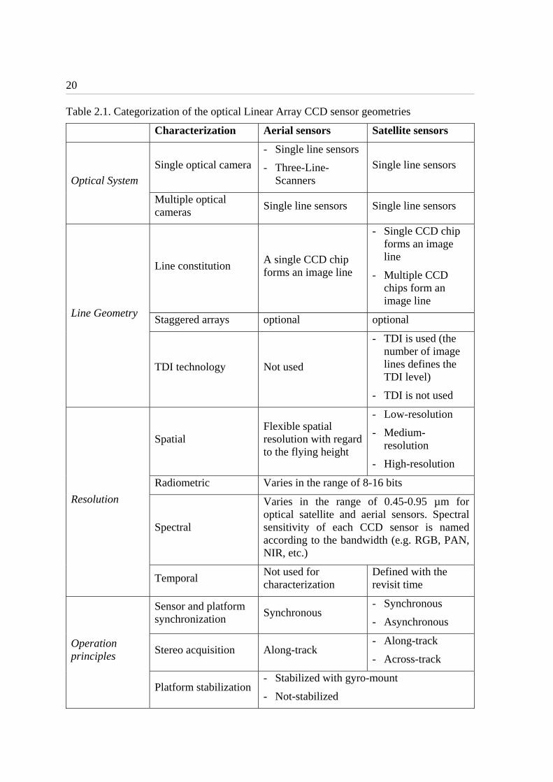
An overview of the Linear Array CCD geometries is given in Table 2.1.

2.1 Optical System Specification

According to the optical systems involved, there are two main design principles: single-lens and multiple-lens systems. For utilization of an aerial/satellite optical sensor in 3D photogrammetric applications, the sensor should have stereo image collection capability. Stereo imaging is possible both in single and multiple lens systems, with the help of platform movement capabilities or the special arrangement of the Linear Array CCD sensors on the focal plane.

High-resolution satellite sensors with single optical system usually work with asynchronous imaging principle, as explained in section 2.4.1, and along-track agile body pointing capability to acquire stereo images in the same orbital pass (e.g. EROS-A of ImageSat Intl., QuickBird of Digital Globe, SPOT-5 HRS of CNES, and IKONOS of GeoEye, etc.).

20

Table 2.1. Categorization of the optical Linear Array CCD sensor geometries

Characterization Aerial sensors Satellite sensors

Single optical camera

- Single line sensors

- Three-Line-Scanners

Single line sensors

Optical System

Multiple optical cameras

Single line sensors Single line sensors

Line constitution A single CCD chip forms an image line

- Single CCD chip forms an image line

- Multiple CCD chips form an image line

Staggered arrays optional optional Line Geometry

TDI technology Not used

- TDI is used (the number of image lines defines the TDI level)

- TDI is not used

Spatial Flexible spatial resolution with regard to the flying height

- Low-resolution

- Medium-resolution

- High-resolution

Radiometric Varies in the range of 8-16 bits

Spectral

Varies in the range of 0.45-0.95 µm for optical satellite and aerial sensors. Spectral sensitivity of each CCD sensor is named according to the bandwidth (e.g. RGB, PAN, NIR, etc.)

Resolution

Temporal Not used for characterization

Defined with the revisit time

Sensor and platform synchronization

Synchronous - Synchronous

- Asynchronous

Stereo acquisition Along-track - Along-track

- Across-track

Operation principles

Platform stabilization - Stabilized with gyro-mount

- Not-stabilized

21

Forward Backward Nadir

Flight direction

In case of the aerial sensors, the Three-Line-Scanner (TLS) design involves a single lens with multiple Linear Array CCDs located on the focal plane for stereo acquisition (Figure 2.1). The ADS40 sensor of Leica, Heerbrugg, the STARIMAGER system of former Starlabo Corporation, Japan, the JAS-150 system of Jena Optronik, Germany, and the HRSC-A and HRSC-AX sensors of DLR, Germany, are examples of aerial TLS sensors.

Satellite sensors with multiple optical systems (cameras), such as Cartosat-1 of ISRO, India, and ALOS/PRISM of JAXA, Japan, etc., can acquire stereo images without body tilting. The image acquisition geometry of ALOS/PRISM sensor is depicted in Figure 2.2 and also in Figure 2.5. The 3-DAS-1 and the 3-OC systems of Wehrli Associates, U.S.A. are the aerial examples of Linear Array CCD sensors with multiple camera heads.

Figure 2.1. A TLS camera operates with pushbroom principle and acquires array images continuously. Multiple image lines with different looking angles are acquired at an instant of time.

2.2 Line Geometry

Several arrangements of the Linear Array CCD chips on the focal plane of a lens can be applied. The arrangements can be classified as following:

- Line constitution: One or more CCD chips can be used to form an image line. The STARIMAGER of the Starlabo and the ADS40 of Leica Geosystems are examples of the sensors with single CCD chips located parallel to the line direction. Alternatively, multiple CCD chips can be employed along a single line with a small overlap and optical butting, as shown in Figure 2.3. Examples of this type of line construction can be found in IRS 1C/1D PAN sensors of ISRO, the IKONOS sensor of GeoEye, the QuickBird sensor of Digital Globe, and the ALOS/PRISM sensor of JAXA. In case of

22

ALOS/PRISM, 6 and 8 Linear Array CCD chips are used to form the image lines of the nadir and forward/backward cameras, respectively.

Figure 2.2. Each camera (forward-nadir-backward) of the ALOS/PRISM acquires one panchromatic image line at time t. All three cameras operate simultaneously and take continuous images of the Earth (t3-t1=t5-t3=45.3).

Figure 2.3. Multiple CCD chips can be located along a single virtual line with a small overlap and optical butting.

- Staggered arrays: Two identical Linear Array CCD chips are located closely in order to improve the ground resolution. Taking one CCD chip as reference, the second CCD chip is shifted by half a pixel in the line direction (Figure 2.4).

Flight direction

Line direction

Forward image

Focal plane of the Backward camera

Satellite orbitNadir image

Backward image

t1 t2

t3 t4 t5 t6

Focal plane of the Nadir camera Focal plane of the

Forward camera

PRISM sensor (ref: www.jaxa.jp)

Forward camera

Backward camera

Nadir camera

23

Figure 2.4. Staggered array structure of the CCD chips.

Examples of staggered array technology can be found in the ADS40 sensor of Leica Geosystems (Reulke et al., 2006) and SPOT missions of CNES. According to Sandau (2003), the spatial resolution can be improved by a factor of 2 when staggered arrays are used in an optimal sampling pattern. However, Becker et al. (2005) analyzed the effect of the staggered arrays into the spatial resolution improvement with ADS40 images. Their investigations show that the improvements are between 8%-15%. Platform motions during the image collection are the main obstacle for the resolution improvement in this case.

- Time Delayed Integration (TDI) technology: Dealing with high-speed image acquisition and processing systems, the speed of operation is often limited by the amount of available light, due to short exposure times. Therefore, high-speed applications often use line-scan cameras, based on CCD sensors with TDI (Bodenstorfer et al., 2007). Depending on the TDI level, a number of Linear Array CCDs are located in parallel, in order to acquire images with improved radiometry. With the TDI technology, a longer effective exposure time is provided without introducing additional motion blur. The TDI is the state-of-the-art and used in a number of high-resolution satellite sensors, such as, the IKONOS, the KOMPSAT-1 and the KOMPSAT-2, the EROS-B, and the WorldView-1.

2.3 Resolution Specification

The term resolution defines the smallest discernable physical unit of an observed signal by a sensor (Kramer, 2002). For the airborne and spaceborne digital optical sensors, one should consider spatial, spectral, temporal, and radiometric resolutions. The primary use of this term in this dissertation refers to the spatial resolution.

2.3.1 Spatial Resolution

Spatial resolution defines the size of an image resolution cell in the target area, or the size of pixels in the focal plane. It is usually expressed in terms of GSD (Ground Sample Distance), footprint, pixel size, or IFOV (Instantaneous Field of View) . The IFOV denotes the (angular) aperture within which the sensor is sensitive to electromagnetic radiation, and it is often expressed as a small solid angle.

The aerial Linear Array CCD sensors can produce images with different GSDs, which are computed with respect to flying height. On the other hand, the earth observation satellite sensors are known with a constant GSD value, even though there might be a deviation

Flight direction

Line direction

24

from this value mainly due to variable convergence angles. Sensors with satellite body movement capability can take images from variable along-track and across-track looking angles and produce different GSDs.

The satellite optical sensor imagery can be classified according to their GSD size. The major classification is done as low, medium and high resolution. The term “very-high resolution” is also used in the literature to point out the sensors with a GSD of better than 5 m. The definitions of the low, medium and high-resolution imagery have always been altered with the availability of the imagery with greater ground resolution. The satellite optical sensors which provide images with a ground resolution of 10 m and better are considered as high-resolution nowadays, while the resolution up to 500 m is classified as medium resolution. Other satellite sensors having a spatial resolution of 500 m and less are considered as low-resolution. Very often, multiple imaging sensors with different spatial resolutions are mounted onboard of one satellite platform.

2.3.2 Radiometric Resolution

The radiometric resolution describes the ability to discriminate very slight differences in energy and represents the sensitivity to detect small differences in reflected or emitted energy. It is expressed by an integer number that corresponds to the number of bits (in power of 2) used to quantize a pixel.

Images provided by line scanners for 3D mapping may have a resolution ranging from 8 bit (256 grey values) to 16 bits (65 566 grey values). Most of satellite and airborne imagers have radiometric resolutions between 8 bits and 12 bits.

2.3.3 Spectral Resolution

The spectral resolution refers to the resolving power of a system in terms of wavelength or frequency (Kramer, 2002). The aerial and satellite Linear Array CCD sensors acquire images usually in panchromatic (PAN) mode and/or in multispectral (MS) mode. These sensors often have multiple Linear Array CCDs with one or more optical camera heads acquiring imagery in different spectral channels. Some sensors, such as IRS 1C/1D, acquire images in a single PAN band covering only a certain part of electromagnetic spectrum (0.50-0.75 m), while some others acquire images in multiple bands, such as IKONOS operating in the PAN (0.50-0.95 m), Blue (0.45-0.52 m), Green (0.51-0.60 m), Red (0.63-0.79 m), and the Near Infrared (0.76-0.85 m) bands. The definitions of the MS bandwidths can differ slightly for different sensors. However, the spectrum definition of PAN band also varies very often, such as the bandwidth is between (0.50-0.90 m) for EROS-A1, (0.49-0.69 m) for Quickbird, (0.45-0.90 m) for GeoEye-1, and (0.50-0.85 m) for Cartosat-2. New band definitions, such as red edge, will be available with the launches of the RapidEye, the Sentinel-2, and the WorldView-2.

Advanced multispectral sensors for remote sensing applications are the hyperspectral sensors, which detect hundreds of very narrow spectral bands throughout the visible, near-infrared, and mid-infrared portions of the electromagnetic spectrum. Their very high spectral resolutions facilitate fine discriminations between different targets based on their spectral response in each of the narrow bands.

25

Panchromatic, RGB (red-green-blue), and near-infrared channels are mainly used in the aerial large format digital cameras. There are also examples of aerial hyperspectal pushbroom sensors, e.g. CASI 1500 and SASI 600 from Itres Research, Canada (www.itres.com, last accessed on 18.01.2008).

2.3.4 Temporal Resolutions of Satellite Sensors

The absolute temporal resolution of a satellite remote sensing system is the time interval between two successive acquisitions of the same area. The temporal resolution is used as an important characteristic for the satellite sensors, since they operate on pre-defined and fixed orbits.

In near-polar orbits, areas at high latitudes will be imaged more frequently than the equatorial zone due to the increasing overlap in adjacent swaths as the orbit paths come closer together near the poles. Some satellite systems can be maneuvered and pointed to the target area to reduce the revisit period. Thus, the actual temporal resolution of a sensor depends on a variety of factors, including the satellite/sensor capabilities, the swath overlap and the latitude.

The ability to collect imagery of the same area of the Earth’s surface at different periods of time is one of the most important characteristics of the remote sensors. Spectral and spatial characteristics of features may change over time and these changes can be detected by collecting and comparing multi-temporal imagery. By imaging on a continuous basis at different times, we are able to monitor the changes that take place on the Earth’s surface, whether they are naturally occurring (such as changes in natural vegetation cover or flooding) or induced by humans (such as urban development or deforestation).

2.4 Operation Principles

Operational principles of the satellite platforms and sensors can be analyzed in two main categories: sensor and platform synchronization and stereo-acquisition principle. When the aerial Linear Array CCD sensors considered, the platform stabilization is a distinctive character of some sensors.

2.4.1 Sensor and Platform Synchronization

According to the sensor and platform synchronization, there are two different operating principles of the satellite sensors:

- Synchronous acquisition mode: The acquisition mode is synchronous if the satellite speed and the scanning speed are equal. Each scan line of a Linear Array CCD is acquired with the same viewing angle. Examples of synchronous image modes are the ALOS/PRISM, Cartosat-1, Orbview-3, etc. Image acquisition principle of the ALOS/PRISM sensor is demonstrated in Figure 2.5.

- Asynchronous acquisition mode: The acquisition mode is asynchronous if the scanning velocity and the platform velocity are not the same (Poli, 2005). Asynchronous imaging is mainly used in the sensors with single optics, in order to

26

acquire along-track stereo images. Examples can be found in Quickbird and EROS-A (Figure 2.6). The image geometries are affected by different off-nadir angles, which cause different sizes of GSDs.

Some satellite sensors, e.g. IKONOS, can operate in both synchronous and asynchronous acquisition modes. The stereo image acquisition is performed using agile body pointing and asynchronous operation capabilities.

Figure 2.5. Image acquisition principle of the PRISM sensor (Tadono et al., 2004)

Figure 2.6. EROS A1 sensor, asynchronous image acquisition, scan angles and the real

shape of the imaged geographical area. (http://imagesat.pionet.com)

27

2.4.2 Stereo Acquisition

Considering the stereo acquisition, there are two main streams:

- Along-track stereo acquisition: In case of satellite sensors with along-track stereo capability, the stereo images of the same area are taken along the flight direction, with a time delay in the order of seconds. Images acquired by successive orbits may have a small overlap in the across-track direction, too. The main advantage of the along-track stereo acquisition (quasi-simultaneous imaging) over the across-track stereo acquisition (on different dates) appears on the radiometric differences of the stereo images. The radiometric image variations, which can be caused by temporal changes, sun illumination, etc., are relatively small between the along-track images. SPOT-HRS, IKONOS, ALOS/PRISM (Figure 2.5), Cartosat-1, EROS-B, and EROS-A1 sensors are examples of along-track stereo image acquisition. All large format aerial Linear Array CCD sensors acquire along-track stereo images.

- Across-track stereo-acquisition: In across-track configuration, the CCD lines and the optical system are combined with a mirror that rotates from one side of the sensor to the other across the flight direction. The along-track angle is constant and close to zero. The across-track angle is usually up to 30°, but can reach larger values (for example 45° with Orbview-3). The number of strips is equal to the number of channels (one for each CCD line), all looking in the same direction. At the next satellite pass over the area of interest, the strips are acquired with a different viewing angle. According to this configuration, the stereo images are collected from different orbits, with the overlapping area across the flight direction (Poli, 2005). The most relevant consequence of this configuration is that the time interval between the acquisitions of two stereo scenes can be in the order of days or more, therefore differences in the land cover, due to natural events or human actions, in weather, and in the cloud distribution may occur. KOMPSAT-1, SPOT-5 HRG, ALOS/AVNIR-2, and RapidEye are examples of the sensors for across-track stereo acquisition. Across-track stereo acquisition with the RapidEye constellation is demonstrated in Figure 2.7.

A few of the high-resolution satellite platforms and sensors has the capability to operate in both modes due to sensor agility. Examples of such sensors in operation and planned for launch in near future are Quickbird, Orbview-3, ResourceSat-1, Formosat-2, KOMPSAT-2, Cartosat-2, GeoEye-1, WorldView-1, WorldView-2, EROS-C, Pleiades-1, and Pleiades-2.

2.4.3 Platform Stabilization

The aerial Linear Array sensors are often stabilized using a gyro-mount in order to reduce the image deformation caused by the aircraft movement and to keep the viewing angle. In comparison to the aircrafts, the satellite platforms operate in a smoother fashion. Therefore, the use of gyro-mount may not be necessary.

As an example, the STARIMAGER sensor (formerly called TLS) uses a high-performance stabilizer, especially since it was initially mounted on a helicopter. The stabilizer has a

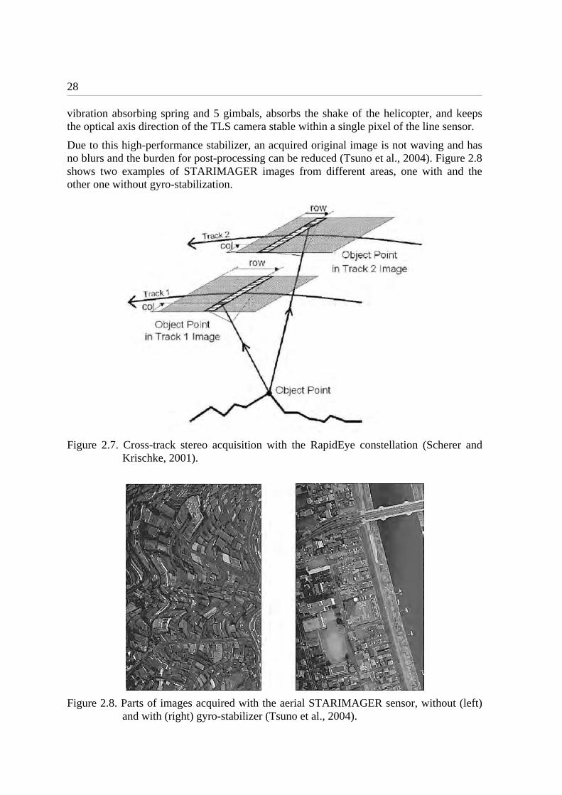
28

vibration absorbing spring and 5 gimbals, absorbs the shake of the helicopter, and keeps the optical axis direction of the TLS camera stable within a single pixel of the line sensor.

Due to this high-performance stabilizer, an acquired original image is not waving and has no blurs and the burden for post-processing can be reduced (Tsuno et al., 2004). Figure 2.8 shows two examples of STARIMAGER images from different areas, one with and the other one without gyro-stabilization.

Figure 2.7. Cross-track stereo acquisition with the RapidEye constellation (Scherer and Krischke, 2001).

Figure 2.8. Parts of images acquired with the aerial STARIMAGER sensor, without (left) and with (right) gyro-stabilizer (Tsuno et al., 2004).

3

CALIBRATION PARAMETERS for the LINEAR ARRAY CCD SENSORS

The interior orientation parameters of a Linear Array CCD sensor are usually determined with a laboratory calibration method. However, these parameters might be altered by time during the operation, which causes systematic errors in image coordinates. A refinement or in-flight calibration is usually necessary to update the given camera calibration data.

Systematic error components of Linear Array CCD sensors encompass camera systematic errors and sensor misalignment and displacements with respect to exterior orientation measurement devices. These components might not be separable due to high correlations among them. Therefore, only a reduced set of components are introduced into bundle adjustment as additional parameters. Often, a parameter corrects errors with similar mathematical effect, e.g. camera constant and the height offset.

This chapter aims to explain only the most common systematic errors of the interior orientation for the Linear Array CCD sensors. These systematic errors can be categorized as optical system (lens) related and the CCD line related parameters. The errors in CCD lines and lens distortions have been described also in another doctoral dissertation by Poli (2005).

3.1 Optical System Related Parameters

The well-known systematic error parameters of the sensor optical systems include lens distortions, change in focal length, and the principal point offset. These parameters are lens specific and if multiple lenses are employed in sensor design, one set of parameters should be defined for each lens separately.

30

3.1.1 Principal Point Displacement

The principal point is defined as “that point on the image plane which is at the base of the perpendicular from the ‘centre of the lens’, or more correctly, from the rear nodal point” (Atkinson, 1996). The length of that perpendicular is the principal distance and, at infinity focus, it is equal to the focal length of the lens (Clarke et al., 1998).

The camera parameters (principal point and the lens distortion) is calibrated in a laboratory with the help of an optical goniometer. In an idealized lens model, the image plane is exactly perpendicular to the optical axis. In reality, there is a slight difference. The point where the optical axis intersects the image plane is called principal point of autocollimation (PPA). The center of the lens distortions refers to the point, where the principal ray of best symmetry intersects the image plane. This point is called principal point of best symmetry (PBS). The image coordinates are referred to the PBS. The mathematical projection centre is at a distance c from PBS (Kraus, 1993).

Systematic errors in the principal point definition cause constant corrections (xp, yp) in the image coordinates of all points.

3.1.2 Camera Constant

The principal distance is called also as camera constant and both terms are equal to camera focal length at infinity focus. Here, all three terms are used identically. The correction term for the camera constant describes any changes in the given parameter of the optical system. A systematic error in the camera constant creates a scale effect in the resulting image coordinates, in case of flat terrain (Figure 3.1). The effect of a change c in the focal length on the image coordinates of a point i are computed using the Equation set 3.1. The

cx and cy represent the correction terms for xi and yi, respectively.

cc

xxx

pi

c )(

cc

yyy

pi

c )(

where, c is the focal length, c is the change in the focal length, xi, yi are the image coordinates of each point, xp, yp are the image coordinates of the principal point of the lens.

3.1.3 Lens Distortions

The widely used definitions of the lens systematic distortions include the radial symmetric lens distortion and the decentering distortion parameters. The Brown (1971) model is used here to correct the systematic errors in the image coordinates caused by the lens distortion.

The radial symmetric distortion is represented as power series of the radial distance r:

...73

52

31 rKrKrKr

(3.1)

(3.2)

31

where, r2 =(x-xp) 2 +(y-yp)

2 and, xp, yp are calibrated image coordinates of the principal point (PBS) of the lens.

In wide-angle and fish-eye lenses, the first three terms (K1, K2, K3) are needed to model the radial symmetric lens distortion of the digital cameras. After the corrections, the error correction terms regarding the radial symmetric lens distortion (xk, yk) on the image coordinates xi, yi of a point i is computed using the Equation set 3.3.

Figure 3.1. Effect of the systematic change in the camera constant. H: flying height, PP: principal point, c: calibrated focal length, c’: erroneous focal length

xk = (xi-xp)ri2k1 + (xi-xp)ri

4k2 +(xi-xp)ri6k3

yk = (yi-yp)ri2k1 + (yi-yp)ri

4k2 +(yi-yp)ri6k3

The first two parameters (p1, p2) of the decentering distortion model defined by Brown (1976) bring corrections (xd, yd) to image coordinates xi, yi of a point i as:

xd = (ri2 +2(xi-xp)

2 )p1 +2(xi-xp) (yi-yp)p2

yd = (ri2 +2(yi-yp)

2 )p2 +2(xi-xp)(yi-yp)p1

For the Linear Array CCD sensors, if no camera calibration data is provided, it is assumed that the xi=xp (equal to zero) for the nadir view. With the camera calibration data, xp = yp= 0 in the beginning of the adjustment. In the subsequent steps, these parameters are replaced

(3.3)

(3.4)

Nominal Flight direction

Camera lens

Image line on the ground

H

Focal plane c c

PP

Focal plane

PP

32

with estimated principal point displacement correction term to obtain corrected image coordinates.

3.2 CCD Line Related Parameters

As shown in Chapter 2.2, an image line can be formed using one or more CCD chips. The systematic error parameters presented here, i.e. scale, rotation, displacement from the principal point, and bending, are in general defined per CCD image line (Figure 3.2). If multiple CCD chips are used to form an image line, it might be necessary to define calibration parameters per CCD chip instead of image line.

3.2.1 Scale effect

The scale effect parameter represents any change in the size of CCD pixel detectors (Figure 3.2a). Systematic errors in CCD detector size and in camera constant have similar influences on the image coordinates. If multiple image lines are located on the focal plane, such as in the Three-Line-Scanners, it might be necessary to introduce one scale parameter for each line. The scale parameter has a significant effect on the y coordinates of the image points, which is defined perpendicular to the flight direction. The correction term for each point i is computed using the Equation 3.5.

ys = -(yi-yp)s

where ys is the resulting correction term on image coordinate yi of each point in y direction, s is the scale parameter for each CCD chip, yp is the image coordinate of the principal point of the lens in y direction.

3.2.2 Rotation

In the pushbroom sensors, the CCD lines are assumed to be perpendicular to the flight direction. However, small rotations might occur during manufacturing. This rotation should be considered in the calibration model. If only one image line is located in the focal plane, i.e. forward, nadir, and backward cameras of the ALOS/PRISM, the line rotation parameter might not be separable from the yaw error of image trajectory. A graphical representation of CCD line rotation is given in Figure 3.2b.

The effect of the CCD line rotation is significant in the x direction. The correction term regarding the CCD line rotation ( x ) for any image point i is computed using the

Equation 3.6.

)y-(y pix

where, yi is the image coordinate of each point in y direction, yp is the image coordinate of the principal point of the lens in y direction, and

(3.6)

(3.5)

33

= 180/π,

)( .

Figure 3.2. (a) Effect of a change in CCD detector size (scale effect). The (x,y) axes represent the image coordinate system, PP is the principal point, l and l are the calibrated and given (uncalibrated or determined in a former calibration method, e.g. using laboratory calibration) positions of a CCD line, respectively.

(b) CCD line rotation in the focal plane. and represent the calibrated and the given rotations of a CCD line, respectively.

(c) CCD line bending in the focal plane.

(d) CCD chip displacements with respect to the principal point. C1, C2, and C3 are calibrated, and C1, C2, and C3 are the given positions of the CCD chip centers.

l

PP

l

y

x

(a)

(c)

l

PP

l

y

x PP

C1

y

x

C3

C2

C1

C3

C2

(d)

l

PP

l

y

x

(b)

34

3.2.3 Displacement from the Principal Point

The center of a CCD line or the individual CCD chips which form an image line are in general displaced from the principal point of the camera. The positions of the CCD chip centers with respect to the principal point should be known for a precise point positioning process. Figure 3.2d demonstrates a change from the given calibration parameters, which can be estimated through self-calibration.

A pair of displacement parameters (xp, yp) is defined for each individual CCD chip. Image coordinates (xi,yi) of each CCD pixel i are updated by adding the estimated (xp, yp) parameters of the corresponding chip.

3.2.4 Bending

A bending error in the Linear Array CCDs forms an arc on the line (Figure 3.2c). The parameter is mainly effective in the x coordinate of the image points. The correction term (xb) for each point i is computed using the Equation 3.7.

xb = (yi-yp)ri2b

where b is the CCD line bending, yi is the image coordinate of each point in y direction, yp is the image coordinate of the principal point of the lens in y direction, and

ri2 =(xi-xp)

2 +(yi-yp) 2

(3.7)

4

METHODOLOGY FOR SENSOR ORIENTATION AND CALIBRATION

Solutions for the georeferencing problem of the imagery of the Linear Array CCD sensors employ both existing and also new photogrammetric algorithms. For accurate georeferencing, the image trajectory should be recorded by external measurement devices, such as GPS, INS, star tracker, etc. The given (measured) trajectory very often contains systematic errors, such as constant positional and rotational displacements, drift in time, etc. The trajectory modeling concept is therefore introduced into the bundle adjustment by modifying the conventional collinearity equations.

Three different trajectory models have been developed and implemented at the Chair of Photogrammetry and Remote Sensing, ETH Zurich by Gruen and Zhang (2003). The models, named as the DGR, the PPM and the LIM, are explained in detail in the following sections. The DGR is applied to the imagery of all sensors in Chapter 5 and validated using reference data. When compared to the DGR, the PPM and the LIM are more complex models. The LIM is applied only in the aerial TLS data, where the image trajectory is comparably uneven due to relatively rough aircraft movements, and sudden changes and jumps can be expected. Therefore, dense orientation fixes might be necessary to model the trajectory errors. On the contrary, the Earth observation satellites move in a smooth orbit and a small number of segments would be adequate for modeling the trajectory errors. With LIM, at least four orientation fixes should be defined with the current implementation of the model. Therefore, the PPM and the DGR are applied to the satellite image data (i.e. ALOS/PRISM) and the use of LIM is avoided.

The airborne optical sensors used here are working with the Three-Line-Scanner (TLS) principle (see Figure 2.1 in Chapter 2). The term TLS refers to the airborne linear array CCD sensors with single lens and three parallel CCD lines located on the focal plane. Although two images of an area acquired from two Linear Array CCDs with different

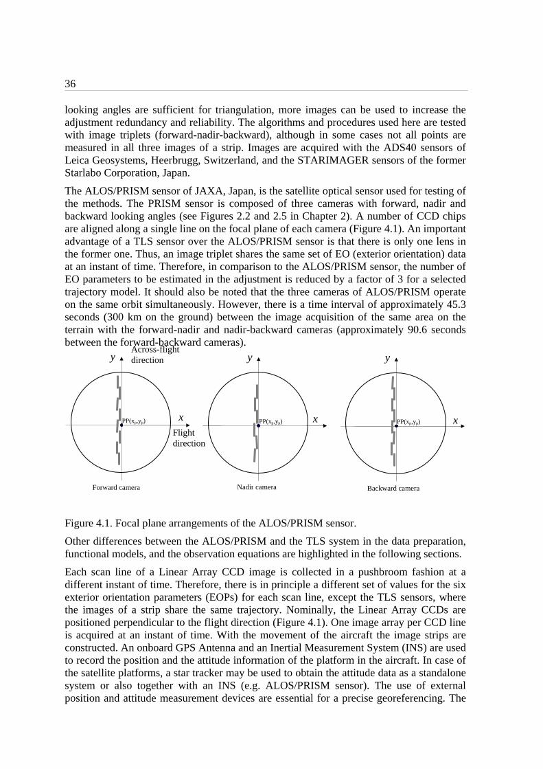
36

looking angles are sufficient for triangulation, more images can be used to increase the adjustment redundancy and reliability. The algorithms and procedures used here are tested with image triplets (forward-nadir-backward), although in some cases not all points are measured in all three images of a strip. Images are acquired with the ADS40 sensors of Leica Geosystems, Heerbrugg, Switzerland, and the STARIMAGER sensors of the former Starlabo Corporation, Japan.

The ALOS/PRISM sensor of JAXA, Japan, is the satellite optical sensor used for testing of the methods. The PRISM sensor is composed of three cameras with forward, nadir and backward looking angles (see Figures 2.2 and 2.5 in Chapter 2). A number of CCD chips are aligned along a single line on the focal plane of each camera (Figure 4.1). An important advantage of a TLS sensor over the ALOS/PRISM sensor is that there is only one lens in the former one. Thus, an image triplet shares the same set of EO (exterior orientation) data at an instant of time. Therefore, in comparison to the ALOS/PRISM sensor, the number of EO parameters to be estimated in the adjustment is reduced by a factor of 3 for a selected trajectory model. It should also be noted that the three cameras of ALOS/PRISM operate on the same orbit simultaneously. However, there is a time interval of approximately 45.3 seconds (300 km on the ground) between the image acquisition of the same area on the terrain with the forward-nadir and nadir-backward cameras (approximately 90.6 seconds between the forward-backward cameras).

Figure 4.1. Focal plane arrangements of the ALOS/PRISM sensor.

Other differences between the ALOS/PRISM and the TLS system in the data preparation, functional models, and the observation equations are highlighted in the following sections.

Each scan line of a Linear Array CCD image is collected in a pushbroom fashion at a different instant of time. Therefore, there is in principle a different set of values for the six exterior orientation parameters (EOPs) for each scan line, except the TLS sensors, where the images of a strip share the same trajectory. Nominally, the Linear Array CCDs are positioned perpendicular to the flight direction (Figure 4.1). One image array per CCD line is acquired at an instant of time. With the movement of the aircraft the image strips are constructed. An onboard GPS Antenna and an Inertial Measurement System (INS) are used to record the position and the attitude information of the platform in the aircraft. In case of the satellite platforms, a star tracker may be used to obtain the attitude data as a standalone system or also together with an INS (e.g. ALOS/PRISM sensor). The use of external position and attitude measurement devices are essential for a precise georeferencing. The

x

Nadir camera

y

PP(xp,yp)

Forward camera

y

PP(xp,yp)

y

PP(xp,yp)

Backward camera

x x Flight direction

Across-flight direction

37

image trajectory, which contains the EO data of each line, is generated from the GPS and INS/star tracker measurements in a post-processing procedure.

The self-calibration is an alternative method to the laboratory and testfield calibration for the calibration of optical imaging systems in the photogrammetric community. It includes mathematical definitions of potential systematic errors of sensors and other system components. These errors are introduced as additional parameters and estimated in the bundle adjustment procedure together with other unknowns (i.e. EOPs, object space coordinates of points). In case of laboratory calibration, the camera interior orientation and distortion parameters are measured using auxiliary devices in a laboratory environment. On the other hand, the testfield calibration is accomplished by acquiring data over specially designated testfields. A regular bundle adjustment (without additional parameters) is applied to obtain image residuals, which are used for determination and analysis of systematic errors in image space.

In this study, the three trajectory models are expanded for self-calibration. The functional model of additional parameters are defined for the aerial TLS sensors and the ALOS/PRISM sensor separately.

Details of the triangulation and the self-calibration procedures are explained in the following sections of this chapter. Solution algorithms of the bundle adjustment system and accuracy evaluation methods are given accordingly.

4.1 Preparation for Rigorous Sensor Orientation

The data provided by the camera vendors and satellite operators are usually presented in a variety of formats. The data should be converted into the input format of the developed models. The major steps of data preparation can be categorized as image trajectory and interior orientation extraction, and coordinate system transformations (pixel-to-image space and between the object space systems). There are some other preparation steps of bundle adjustment that are not covered here, such as GCP ground and image measurements, image format extraction, image preprocessing, etc.

4.1.1 Image Trajectory Extraction

The image trajectory data contain the EOPs of each image line. The given trajectory data should refer to the perspective center of the camera. Trajectory extraction for each image line regards to post-processing of the position and attitude measurement devices, coordinate transformation, sensor alignment correction, and time integration including data interpolation. In case of the satellite imagery, orbital data extraction can be part of the process as well.

The EOPs of the aerial Linear Array imagery are measured using GPS and INS instruments. A specially designed Kalman Filter is often applied for integration of the GPS/INS data. The data output rates of the GPS devices are lower than the image scan rate (i.e. 5 Hz vs. 500 Hz, respectively). An INS comprises multiple IMUs (Inertial Measurement Units), which measure the attitude and acceleration of a platform. There is a variety of IMUs, with different data output frequencies and accuracy levels. The post-

38

processing of GPS/INS data with the Kalman Filter increases the overall accuracy of the system. As a part of the data integration process, coordinate system transformations might be necessary to bring different sources of data into the same coordinate system, such as from inertial reference system and the GPS system to the camera system, which has the origin in the perspective center of the camera. These transformations include sensor misalignment parameters and positional displacements.

It is often necessary to interpolate the output trajectory data to compute the EOPs of each image line. For example, in case of the ALOS/PRISM imagery, the EO (exterior orientation) values are given in certain periods of time, i.e. every 1 second for attitude, etc. Instead of a simple linear interpolation, a polynomial function, such as Lagrange polynomials, is preferred to improve the interpolation accuracy.

Alternatively, the orbit of a satellite can be defined with Keplerian elements or state vectors. The Keplerian elements are composed of six elements: semi-major axis, inclination, argument of perigee, eccentricity, true anomaly, and right ascension of ascending node. The state vectors contain position, attitude and velocity of the satellite for a particular time. However, these two approaches have not been employed in this study.

4.1.2 Interior Orientation Extraction

The interior orientation data of the Linear Array CCD imagery refers to the location of each CCD pixel (x, y) in the image coordinate system and the focal length of the camera. In the practical implementation of the TLS-LAB software, a look-up table, which contains the position parameters (x,y) of each CCD detector with regard to the principal point, is used for transformation of measured pixel coordinates into image space coordinates. If the given interior orientation data is expressed as a set of sensor parameters, such as lens distortion parameters, number of CCD pixel detectors, pixel size, CCD line inclination, etc., these parameters should be transformed into a look-up table for being input into the software. Another problem of interior orientation extraction might appear in the coordinate transformation. If the given parameters are defined in a reference system other than the image coordinate system, e.g. the PRISM pixel positions, they should be transformed into the image system accordingly.

4.1.3 Coordinate System Transformations

4.1.3.1 Transformations Among Object Space Coordinates

The basic collinearity equation in photogrammetry is in principle a similarity transformation for each imaging ray and should be performed in a Cartesian coordinate system. If camera perspective center coordinates (i.e. EOPs) and GCP ground coordinates are given in different systems, they are transformed into a Cartesian reference system. If the coordinates are referenced to a projection system, such as geographical coordinates, the Universal Transverse Mercator (UTM), etc., a local coordinate system can be defined by the user.

39

The planimetric coordinates of the GCPs used in the practical applications of this study are mostly given in either the UTM projection system or the geographical coordinates (latitude and longitude). The height values are referenced to the ellipsoidal or geoid surfaces.

The image trajectory data of the aerial Linear Array CCD sensors are usually provided in the UTM projection system. In the case of the ALOS/PRISM sensor, the trajectory data are defined in two different reference systems. The attitude data are presented as 4 parameter quaternion defined in the ECI (Earth Centered Inertial) system. A transformation from the given attitude data into the earth fixed coordinate system (ECR- Earth Centered Rotational) is therefore performed by taking the earth rotation into account. The satellite position data are provided both in the ECR and the ECI systems.

In a last step, an additional transformation procedure has been applied to bring the trajectory coordinates and the GCP ground coordinates into the same Cartesian coordinate system, which is a local system and defined per project.

After the bundle adjustment, the following back transformations may be applied to appropriate systems:

The trajectory data may be updated after the bundle adjustment process, and the new trajectory coordinates are transformed into the corresponding projection system.

The ground coordinates of the new (tie) points are transformed from the local coordinate system into the coordinate system in which the GCPs are defined originally.

4.1.3.2 Pixel-Space to Image-Space Transformation

In Linear Array CCD imagery, the pixel coordinates of one certain point are measured by its digital image column v and the scan line number u (Figure 4.2). The origin point of the image coordinate system is defined according to the perspective center (xp, yp, -c) of the camera, where (xp, yp) are the principal point coordinates on the focal plane, and c is the camera constant. The (x,y) are used to denote the image space coordinates of the points. In the following formulations, the x axis is defined parallel to the nominal flight direction (Figure 4.3). The y axis is perpendicular to the x axis. In the ideal case, the y axis shall be parallel to the Linear Array CCD. In practice, there is often a small inclination angle between the y axis and the Linear Array CCDs.

The image coordinates (x, y) of an image point are computed using the pixel coordinate v and the interior orientation parameters. A common approach used to perform pixel-to-image space coordinate transformation for the Linear Array CCD imagery is to estimate the camera interior orientation parameters and lens distortion in the laboratory and to generate a calibration file for each CCD line of the camera accordingly. In case of satellite imagery, the interior orientation parameters change after the launch due to temperature differences. Therefore in-flight calibration through self-calibration is necessary to update the camera calibration data file. The calibration data file contains the camera interior parameters, such as focal length and CCD pixel size, and a look-up table with the image space coordinates (x,y) of the center of each pixel in the CCD array.

40

Figure 4.2. Pixel coordinate system of Linear Array CCD images.

Figure 4.3. Image space (focal plane) coordinate system of TLS cameras. PP denotes the principal point of camera lens and origin of the image coordinate system. As a first approximation, the PP coincides with the center point of the nadir CCD line.

By using the look-up table, the image coordinates of a point i can be computed in sub-pixel level. Having the pixel coordinates (u,v) of the point as input, a linear interpolation is performed between the image coordinates of the centers of two neighboring pixels, as following:

xi =calxk +(calxk+1-calxk) × dv

yi =calyk +(calyk+1-calyk) × dv

where (xi,yi) are the calibrated image space coordinates of a measured point i, which is located between the center points of the two neighboring CCD detectors (k) and (k+1), calxk and calyk are the calibrated coordinates of the centers of pixel k (corresponds to the integer part of measured coordinate v), and dv denotes the decimal (sub-pixel) part of v.

(4.1a)

(4.1b)

Flight (scan) direction

Line direction

u

v

x (nominal flight direction)

y

PP(xp,yp)

Backward CCD Line Nadir CCD Line

Forward CCD Line

41

In case of the STARIMAGER camera, the interior orientation parameters were estimated by a collimator device. The CCD line structure is demonstrated in Figure 4.4. C denotes the center point of the Linear Array CCD, PP is the principal point of the camera, and is the inclination of CCD array to the y-axis.

Figure 4.4. TLS CCD sensor coordinate system definition and interior orientation parameters (Gruen, Zhang, 2002).

The image coordinates (x, y) of a point in STARIMAGER are computed by following equations with respect to its pixel coordinate v:

x = xc + (v-Midv) × ps × sin

y = yc + (v-Midv) × ps × cos

x = x + r × x/r = Ix(v)

y = y + r × y/r = Iy(v)

where r = a1r + a3r3 + a5r

5 r = 22 yx

A correction term (r) for the radial distortion of the camera is included in the transformation. (xc, yc) are the image coordinates of the center of the CCD arrays, is the inclination angle for the CCD arrays to the image y axis, a1, a3 and a5 are radial symmetric lens distortion correction coefficients, Midv is the number of the CCD central pixel, and ps is the pixel size (Gruen and Zhang, 2002).

(4.2)

(4.3)

PP

CCD Pixel number

P

x

y

xi

yi

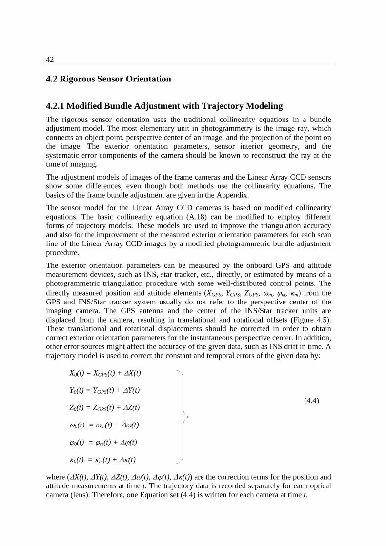
42

4.2 Rigorous Sensor Orientation

4.2.1 Modified Bundle Adjustment with Trajectory Modeling

The rigorous sensor orientation uses the traditional collinearity equations in a bundle adjustment model. The most elementary unit in photogrammetry is the image ray, which connects an object point, perspective center of an image, and the projection of the point on the image. The exterior orientation parameters, sensor interior geometry, and the systematic error components of the camera should be known to reconstruct the ray at the time of imaging.

The adjustment models of images of the frame cameras and the Linear Array CCD sensors show some differences, even though both methods use the collinearity equations. The basics of the frame bundle adjustment are given in the Appendix.

The sensor model for the Linear Array CCD cameras is based on modified collinearity equations. The basic collinearity equation (A.18) can be modified to employ different forms of trajectory models. These models are used to improve the triangulation accuracy and also for the improvement of the measured exterior orientation parameters for each scan line of the Linear Array CCD images by a modified photogrammetric bundle adjustment procedure.

The exterior orientation parameters can be measured by the onboard GPS and attitude measurement devices, such as INS, star tracker, etc., directly, or estimated by means of a photogrammetric triangulation procedure with some well-distributed control points. The directly measured position and attitude elements (XGPS, YGPS, ZGPS, m, m, m) from the GPS and INS/Star tracker system usually do not refer to the perspective center of the imaging camera. The GPS antenna and the center of the INS/Star tracker units are displaced from the camera, resulting in translational and rotational offsets (Figure 4.5). These translational and rotational displacements should be corrected in order to obtain correct exterior orientation parameters for the instantaneous perspective center. In addition, other error sources might affect the accuracy of the given data, such as INS drift in time. A trajectory model is used to correct the constant and temporal errors of the given data by:

X0(t) = XGPS(t) + X(t)

Y0(t) = YGPS(t) + Y(t)

Z0(t) = ZGPS(t) + Z(t)

0(t) = m(t) + (t)

0(t) = m(t) + (t)

0(t) = m(t) + (t)

where (X(t), Y(t), Z(t), (t), (t), (t)) are the correction terms for the position and attitude measurements at time t. The trajectory data is recorded separately for each optical camera (lens). Therefore, one Equation set (4.4) is written for each camera at time t.

(4.4)

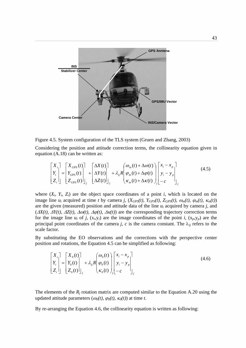
43

Figure 4.5. System configuration of the TLS system (Gruen and Zhang, 2003)

Considering the position and attitude correction terms, the collinearity equation given in equation (A.18) can be written as:

j

pi

pi

jm

m

m

ij

jjGPS

GPS

GPS

i

i

i

c

yy

xx

tt

tt

tt

R

tZ

tY

tX

tZ

tY

tX

Z

Y

X

)()(

)()(

)()(

)(

)(

)(

)(

)(

)(

where (Xi, Yi, Zi) are the object space coordinates of a point i, which is located on the image line ui acquired at time t by camera j, (XGPS(t), YGPS(t), ZGPS(t), m(t), m(t), m(t)) are the given (measured) position and attitude data of the line ui acquired by camera j, and (X(t), Y(t), Z(t), (t), (t), (t)) are the corresponding trajectory correction terms for the image line ui of j, (xi,yi) are the image coordinates of the point i, (xp,yp) are the principal point coordinates of the camera j, c is the camera constant. The ij refers to the scale factor.

By substituting the EO observations and the corrections with the perspective center position and rotations, the Equation 4.5 can be simplified as following:

j

pi

pi

j

ij

ji

i

i

c

yy

xx

t

t

t

R

tZ

tY

tX

Z

Y

X

)(

)(

)(

)(

)(

)(

0

0

0

0

0

0

The elements of the Rj rotation matrix are computed similar to the Equation A.20 using the updated attitude parameters (0(t), 0(t), 0(t)) at time t.

By re-arranging the Equation 4.6, the collinearity equation is written as following:

(4.5)

GPS Anntena

Camera Center

GPS/IMU Vector

INS/Camera Vector

INS Stabilizer Center

(4.6)

44

pjjijjijjij

jijjijjijjij x

ZZrYYrXXr

ZZrYYrXXrcx

tttttt

tttttt

)()()(

)()()(

)()()()()()(

)()()()()()(

033023013

031021011

pjjijjijjij

jijjijjijjij y

ZZrYYrXXr

ZZrYYrXXrcy

tttttt

tttttt

)()()(

)()()(

)()()()()()(

)()()()()()(

033023013

032022012

The ij is canceled out similar to the Equations (A.19a) and (A.19b).

Equations (4.5, 4.6, 4.7a and 4.7b) are the basic equations in the triangulation approach of the Linear Array images, which are appended by a trajectory model. Three different types of trajectory models are investigated by Gruen and Zhang (2003): (a) Direct georeferencing with stochastic exterior orientations (DGR), (b) Piecewise Polynomials with kinematic model up to second order and stochastic first and second order constraints (PPM) and (c) Lagrange Polynomials with variable orientation fixes (LIM). The LIM has been modified in this study. The mathematical definitions of the trajectory models and their observation equations used in the adjustment are given in the following sub-sections.

4.2.1.1 DGR Model

The image trajectory is modeled as a whole with the DGR model. Considering the errors of the aircraft attitude elements and the GPS errors, the positional systematic errors of the trajectory are modeled as:

X0(t) = XGPS(t) +Xoff

Y0(t) = YGPS(t) + Yoff

Z0(t) = ZGPS(t) + Zoff

where (Xoff, Yoff, Zoff) are one set of unknown offset parameters to be estimated for the whole strip.

Similarly, the attitude error terms (, , ) can be modeled by 6 parameters using the following equations for the whole trajectory:

(t) = 0 + 1t

(t) = 0 + 1t

(t) = 0 + 1t

The attitude errors of the INS/Star tracker system mainly consist of the constant offset (0, 0, 0) due to the incorrect initial alignment and the drift errors in time (1, 1, 1). These errors have to be determined or corrected to obtain the correct attitude data at time t (0(t), 0(t), 0(t)).

The EO elements of the collinearity equation are updated in the adjustment after each iteration using:

(4.8)

(4.9)

(4.7a)

(4.7b)

45

X0j = XGPS(t) + Xoff

Y0j = YGPS(t) + Yoff

Z0j = ZGPS(t) + Zoff

0j = m(t) + 0 + 1t

0j = m(t) + 0 + 1t

0j = m(t) + 0 + 1t

The factor t for the attitude drift vector parameters represents the time. In case that the data acquisition time is not recorded, the t can be represented as a function of the pixel coordinate (u) assuming a constant scanning frequency (fs):

sf

ut

When the scan line frequency (fs) information is not available, this term can be replaced by a ratio factor di for each point:

se

sii uu

uud

where ui is the pixel coordinate of a point (i) in the scan line direction, us is the first line of the trajectory part used in the adjustment (if the whole trajectory is used for the adjustment, then us = 0), and ue is the number of last scan line of the trajectory part used for the adjustment.

The observation equations used for the DGR model are:

vc=Axoff + Bsxs + Bdxd + Cxg – lc ; Pc

voff= xoff – loff ; Poff

vs= xs – ls ; Ps

vd= xd – ld ; Pd

vg= xg – lg ; Pg

The first equation of this system is the linearized observation equations of the modified collinearity equations, which are obtained from substitution of the trajectory model parameters given in Equation set 4.10 into the Equations 4.7a and 4.7b. xoff is the unknown positional offset vector; xs and xd are the unknown INS shift and drift terms respectively; xg is the ground coordinates vector; A, Bs, Bd and C are the corresponding design matrices; v, l and P are the respective residual and discrepancy vectors and weight matrices.

(4.13)

(4.10)

(4.12)

(4.11)

46

The total number of the unknown parameters for the DGR model is computed using:

pnsunknowns nnu 39

where ns is total number of image trajectories to model, and npn is the total number of object points. The factor 9 for ns refers to the trajectory unknowns, which are unknown positional offset vector (given in Equation set (4.8): Xoff, Yoff, Zoff), and the INS shift and drift vectors (given Equation set (4.9): 0,0,0, 1,1,1).

The total number of observation equations is computed using:

gcpcsraysnsobservatio nnnn 32

where nrays is number of measured image points (rays), ncs is the number of observation equations used for the trajectory unknowns (9×ns), and ngcp is the number of GCPs, which are used as full-control, in the adjustment. If a GCP is used only as planimetric or as height control point, then only the respective ground coordinates are introduced as weighted observations and the number of constraints for this point is two or one, respectively.

The minimum number of image points and GCPs to be used with the DGR model are listed below for basic image block configurations of two types of sensors. The underlying assumptions for the computations are: all GCPs are full control points, all points are measured in all images with a good distribution, and the EO parameters are free unknowns in the adjustment (apriori EOP >> gcp & EOP >> pixel size).

- For the triangulation of one ALOS/PRISM image triplet, a minimum of 3 full GCPs should be measured for the estimation of the trajectory unknowns (4 is preferred for redundancy). A total of 6 points (GCP + tie) are required for the solution. When the self-calibration is applied, one additional point per image should be measured per AP (e.g. for the 6 AP set, 2 more points should be measured in all 3 images).

- For the triangulation of one TLS image triplet, again a minimum of 3 full GCPs should be measured for estimation of the trajectory unknowns (4 is preferred). When the self-calibration is applied (with 18 APs), a total of 6 points (GCP + tie) are required for the solution.

By substituting the updated EO elements (Equation 4.10) in the collinearity equations (4.7a and 4.7b), the image coordinates (xi, yi) of the point are computed. The discrepancy vector consist of the differences between the image coordinates (xi, yi), which are computed from the collinearity equations, and the measured ones obtained after a transformation from pixel to the image systems ( '' , ii yx ):

lx='ii xx

ly='ii yy

The partial terms of the collinearity equation (A.21a and A.21b), which are fx, fy, and fz, are used for further computation of the elements of the design matrices. The design matrices for image observations are formed as following:

(4.14)

(4.15)

(4.16)

47

232221

131211

aaa

aaaA

232221

131211

bsbsbs

bsbsbsBs

232221

131211

bdbdbd

bdbdbdBd

C =-A

The following equations are used to compute the elements of the design matrix A for each image point i.

z

c

off f

xrcr

X

xa 1311

11

z

c

off f

xrcr

Y

xa 2321

12

z

c

off f

xrcr

Z

xa 3331

13

z

c

off f

yrcr

X

ya 1312

21

z

c

off f

yrcr

Y

ya 2322

22

z

c

off f

yrcr

Z

ya 3332

23

Equation set (4.18a) is used for computations of the a11, a12, a13, which are elements of design matrix A for the xi component of image coordinates, while the equation set (4.18b) is used for computing the a21, a22, a23 elements for the yi component. c denotes the camera focal length, r11…r33 are the elements of the rotation matrix given in Equation set (A.20), and fx, fy, and fz, are the partial terms of the collinearity equation given in Equation set (A.21).

For the x component of the image space coordinates, the following derivatives are used to compute the elements of the Bs matrix:

20

11z

xZzX

f

fdfdc

xbs

20

12z

xZzX

f

fdfdc

xbs

20

13z

xZzX

f

fdfdc

xbs

And for the y component:

(4.18a)

(4.18b)

(4.19a)

(4.17)

48

20

21z

YZYY

f

fdfdc

ybs

20

22z

YZYY

f

fdfdc

ybs

20

23z

YZYY

f

fdfdc

ybs

where;

)(coscoscos

)(cossincos)(cossin

0

00

ji

jijiX

ZZ

YYXXd

)(sincoscos)(sinsincos)(sinsin 000 jijijiY ZZYYXXd

))(sincoscossin(sin

))(sinsincoscos(sin

0

0

ji

jiX

ZZ

YYd

))(coscossinsinsin(

))(cossinsincossin(

0

0

ji

jiY

ZZ

YYd

))(cossinsincos(sin

))(coscossinsinsin()(sincos(

0

00

ji

jijiX

ZZ

YYXXd

))(sinsincoscos(sin

))(sincoscossinsin()(coscos(

0

00

ji

jijiY

ZZ

YYXXd

)(cossin)(sinsin)(cos 000 jijijiZ ZZYYXXd

)(sincos)(coscos 00 jijiZ ZZYYd

0Zd

where c is the camera constant, and fx, fy, and fz are the partial terms of the collinearity equation given in equation set (A.21).

Elements of the design matrix Bd are functions of the elements of the design matrix Bs:

idbsx

bd 111

11

idbsx

bd 121

12

idbsx

bd 131

13

idbsy

bd 211

21

idbsy

bd 221

22

idbsy

bd 231

23

The di coefficient is computed from the Equation 4.12 for each image point (ray) i.

(4.19b)

(4.20)

(4.21)

49

The structural characteristic of the design matrices A, Bs, Bd, and C of Eq. 4.13 are represented in Figure 4.6. The resulting normal equations matrix (N = Qxx

-1 in Eq. A.14) and the solution vector ( x in Eq. A.6) are demonstrated in Figure 4.7. The sample matrices given in both Figures are demonstrated for an ALOS/PRISM image triplet (forward, nadir, and backward images).

lT (discrepancy vector) lc

[image rays 2,1]

loff+ ls+ ld

[3 9,1]

lg

[Full GCP 3,1]

Figure 4.6. The sparsity structure of the design matrix and the discrepancy vector for the DGR model, demonstrated for an ALOS/ PRISM image triplet.

A + Bs + Bd

Forwardimage

9

Nadir image

9

Backward image

9

C Pn3

A + Bs + Bd

A + Bs + Bd P1

P2

Pn-1

Pn

Image rays 2

3 9

Full GCP 3

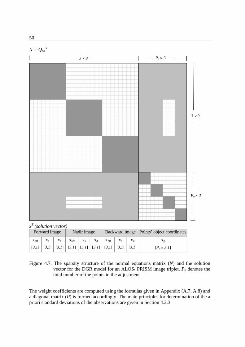
50

N = Qxx-1

xT (solution vector) Forward image Nadir image Backward image Points’ object coordinates

xoff

[3,1]

xs

[3,1]

xd

[3,1]

xoff

[3,1]

xs

[3,1]

xd

[3,1]

xoff

[3,1]

xs

[3,1]

xd

[3,1]

xg

[Pn 3,1]

Figure 4.7. The sparsity structure of the normal equations matrix (N) and the solution vector for the DGR model for an ALOS/ PRISM image triplet. Pn denotes the total number of the points in the adjustment.

The weight coefficients are computed using the formulas given in Appendix (A.7, A.8) and a diagonal matrix (P) is formed accordingly. The main principles for determination of the a priori standard deviations of the observations are given in Section 4.2.3.

3 9

Pn 3

3 9 Pn 3

51

4.2.1.2 Piecewise Polynomial Model

The piecewise polynomial model is used to model the image trajectory with respect to time (Lee et al. 2000). In this model, the values of the exterior orientation parameters are written as polynomial functions of time. The bundle adjustment solution determines the polynomial coefficients instead of the exterior orientation parameters themselves. Due to the instability of the high-order polynomial models, the piecewise polynomial model is used, in which the full complex trajectory is divided into sections, with each section having its own set of low-order polynomials. Continuity constraints on the orientation parameters at the section boundaries ensure that the calculated positions and attitudes are continuous across the boundaries. The piecewise polynomial model is used to model the position and attitude errors (given in Eq. 4.4: X, Y, Z, , , ) with respect to time. The model is described as:

2210)( txtxxtX kkk

2210)( tytyytY kkk

2210)( tztzztZ kkk

2210)( ttt kkk

2210)( ttt kkk

2210)( ttt kkk

for k=1,2,…,ns (ns = number of polynomial segments)

The given trajectory data is updated in the bundle adjustment after each iteration, using the

estimated unknowns ( kkkkkkkkkkkkkkkkkkk zyxzyxzyx 2222111000222111000 ,,,,,,,,,,,,,,,,, );

(k=1,2,…, ns) as following:

22100 )( txtxxtXX kkk

GPSj

22100 )( tytyytYY kkk

GPSj

22100 )( tztzztZZ kkk

GPSj

22100 )( ttt kkk

INSj

22100 )( ttt kkk

INSj

22100 )( ttt kkk

INSj

where se

s

uu

uut

(4.22)

(4.23)

52

k represents the polynomial segment number, u is the pixel space coordinate of a measured point in scan line direction, and us and ue are the begin line and end line numbers of the polynomial segment k, respectively.

There are two kinds of constraints that are applied to each parameter at the section boundaries. The zero order continuity constraints ensure that the value of the function computed from the polynomial in every two neighboring sections is equal at their boundaries, i.e.

2210

212

11

10 txtxxtxtxx kkkkkk

2210

212

11

10 tytyytytyy kkkkkk

2210

212

11

10 tztzztztzz kkkkkk

2210

212

11

10 tttt kkkkkk

2210

212

11

10 tttt kkkkkk

2210

212

11

10 tttt kkkkkk

where k=2,3,…,ns

The first order continuity constraint requires that the slope, or first order derivatives of the functions in two adjacent sections is forced to have the same value at their boundary, i.e.

txxtxx kkkk21

12

11 22

tyytyy kkkk21

12

11 22

tzztzz kkkk21

12

11 22

tt kkkk21

12

11 22

tt kkkk21

12

11 22

tt kkkk21

12

11 22

k=2,3,…,ns

With the PPM, the bundle adjustment solution determines the polynomial coefficients instead of the exterior orientation parameters themselves. The overall estimation model results in:

(4.24)

(4.25)

53

vc = Axpos + Bxatt + Cxg – lc ; Pc

vpos= xpos – lpos; Ppos

vA2=A1xpos – lA1; PA1

vA3=A2xpos – lA2; PA2

vatt= xatt – latt; Patt

vB2= B1xatt – lB1; PB1

vB1= B2xatt – lB2; PB2

vg = xg – lg ; Pg

where the first equation of this system is the linearized observation equations of the modified collinearity equations, which are obtained from substitution of the trajectory model parameters given in Equation set 4.23 into the Equations 4.7a and 4.7b. The following equations are derived from the two kinds of constraints; xpos contains the unknown positional correction terms (X, Y, Z) for all sections; xatt is the unknown attitude error vector (, , ) for all sections; xg is the ground coordinate vector; A, A1, A2, B, B1, B2, and C are the corresponding design matrices; v, l and P are the respective residual and discrepancy vectors and weight matrices. Through this consequent weighting scheme much flexibility is obtained with respect to the modeling of different trajectory conditions.

The number of unknowns in this model is computed by:

pn

n

ipiecesunknowns nnu

s

i318

1

where ns is the total number of image trajectories to model, npieces is the number of polynomial pieces (segments), and npn is the total number of object points. 18 is the number of polynomial coefficients per trajectory segment.

The number of observation equations is computed with:

gcpcsraysnsobservatio nnnn 32

where nrays is number of measured image points (rays), ngcp is number of full ground control points in the adjustment. The number of observation equations (ncs) contains three different kinds of constraints. The zero and first order continuity constraints (Eq. 4.24 and 4.25) are applicable when the trajectory is divided into multiple segments. In addition, the trajectory unknowns are introduced as weighed observations (vpos and vatt in Eq. 4.26) into the adjustment in order to increase modeling flexibility and also to increase adjustment stability . In case of multiple trajectory segments, the ncs is computed using:

s

i

s

i

n

ipieces

n

ipiecescs nnn

11

)1(1218

If the trajectory is modeled as a whole, the last term of the equation above becomes zero.

(4.27)

(4.28)

(4.26)

(4.29)

54

The minimum number of image points and GCPs to be used in the adjustment with the PPM with one segment are listed below for the basic image block configurations of the two sensor types. The underlying assumptions for the computations are: all GCPs are full control points, all points are measured in all images with a good distribution, and the EO parameters are free unknowns in the adjustment (apriori EOP >> gcp & EOP >> pixel size).

- For the triangulation of one ALOS/PRISM image triplet, a minimum of 6 full GCPs should be measured for determination of 18 trajectory unknowns. A total of 13 points (GCP + tie) are required for the solution for the triplet. When the self-calibration is applied, one additional point (of any type) per image should be measured per AP (e.g. for the 6 AP set, 2 more points should be measured in all 3 images).

- For the triangulation of one TLS image triplet, again at least 6 full GCPs should be measured for determination of 18 trajectory unknowns. When the self-calibration is applied (with 18 APs), a minimum of 7 points (GCP + tie) are required for the solution.

The design matrices are formed for each image point i as following:

292827262524232221

191817161514131211

aaaaaaaaa

aaaaaaaaaAi

292827262524232221

191817161514131211

bbbbbbbbb

bbbbbbbbbBi

The elements of the first three columns of the A and B matrices are computed using equations (4.18) and (4.19). The remaining elements are computed with:

21

11

24

14

a

at

a

a

22

12

25

15

a

at

a

a

23

13

26

16

a

at

a

a

21

112

27

17

a

at

a

a

22

122

28

18

a

at

a

a

23

132

29

19

a

at

a

a

21

11

24

14

b

bt

b

b

22

12

25

15

b

bt

b

b

23

13

26

16

b

bt

b

b

21

112

27

17

b

bt

b

b

22

122

28

18

b

bt

b

b

23

132

29

19

b

bt

b

b

(4.31)

(4.30)

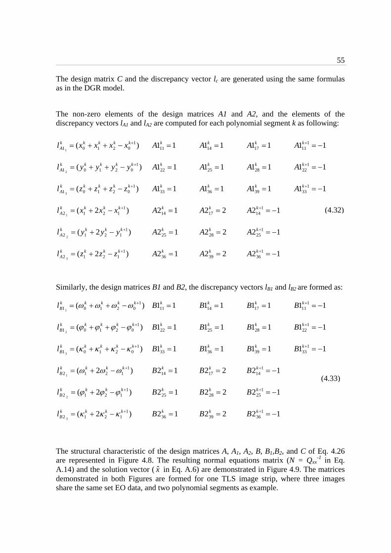
55

The design matrix C and the discrepancy vector lc are generated using the same formulas as in the DGR model.

The non-zero elements of the design matrices A1 and A2, and the elements of the discrepancy vectors lA1 and lA2 are computed for each polynomial segment k as following:

)( 1021011

kkkkkA xxxxl 1111

kA 1114 kA 1117

kA 11 111 kA

)( 102101 2

kkkkkA yyyyl 1122

kA 1125 kA 1128

kA 11 122 kA

)( 102101 3

kkkkkA zzzzl 1133

kA 1136 kA 1139

kA 11 133 kA

)2( 11212 1

kkkkA xxxl 1214

kA 2217 kA 12 1

14 kA

)2( 11212 2

kkkkA yyyl 1225

kA 2228 kA 12 1

25 kA

)2( 11212 3

kkkkA zzzl 1236

kA 2239 kA 12 1

36 kA

Similarly, the design matrices B1 and B2, the discrepancy vectors lB1 and lB2 are formed as:

)( 1021011

kkkkkBl 1111

kB 1114 kB 1117

kB 11 111 kB

)( 102101 2

kkkkkBl 1122

kB 1125 kB 1128

kB 11 122 kB

)( 102101 3

kkkkkBl 1133

kB 1136 kB 1139

kB 11 133 kB

)2( 11212 1

kkkkBl 1214

kB 2217 kB 12 1

14 kB

)2( 11212 2

kkkkBl 1225

kB 2228 kB 12 1

25 kB

)2( 11212 3

kkkkBl 1236

kB 2239 kB 12 1

36 kB

The structural characteristic of the design matrices A, A1, A2, B, B1,B2, and C of Eq. 4.26 are represented in Figure 4.8. The resulting normal equations matrix (N = Qxx

-1 in Eq. A.14) and the solution vector ( x in Eq. A.6) are demonstrated in Figure 4.9. The matrices demonstrated in both Figures are formed for one TLS image strip, where three images share the same set EO data, and two polynomial segments as example.

(4.32)

(4.33)

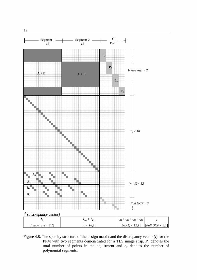
56

lT (discrepancy vector) lc

[image rays 2,1]

lpos+ latt

[ns 18,1]

lA1+ lA2+ lB1+ lB2

[(ns -1) 12,1]

lg

[Full GCP 3,1]

Figure 4.8. The sparsity structure of the design matrix and the discrepancy vector (l) for the PPM with two segments demonstrated for a TLS image strip. Pn denotes the total number of points in the adjustment and ns denotes the number of polynomial segments.

A + B

Segment-1 18

Segment-2 18

C Pn3

A + B

P1

P2

Pn-1

A1

A2

B1

B2

Pn

Image rays 2

ns 18

Full GCP 3

(ns -1) 12

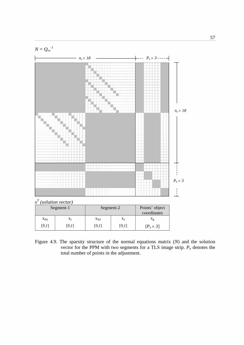
57

N = Qxx-1

xT (solution vector) Segment-1 Segment-2 Points’ object

coordinates xdis

[9,1]

xs

[9,1]

xdis

[9,1]

xs

[9,1]

xg

[Pn 3]

Figure 4.9. The sparsity structure of the normal equations matrix (N) and the solution vector for the PPM with two segments for a TLS image strip. Pn denotes the total number of points in the adjustment.

ns 18

Pn 3

ns 18 Pn 3

58

4.2.1.3 Lagrange Interpolation Model (LIM)

Ebner et al. (1992) developed the principle of orientation images or orientation fixes for the geometric in-flight calibration of MOMS imagery. This method is based on collinearity equations and the exterior orientation parameters are determined in the so-called orientation fixes, which are introduced at certain time intervals. Between the orientation fixes, the exterior orientation parameters of an arbitrary scan line are interpolated using Lagrange polynomials. All unknown orientation parameters for these orientation fixes are estimated in a least squares adjustment procedure, and the parameters for each individual scan line are interpolated with its neighboring orientation fixes. The general form of the nth order Lagrange polynomial is given as:

n

ijj ji

jn

iin tt

tttPtP

;00

)()(

Where Pn(t) at time t is interpolated from the values P(ti) at the n+1 neighboring orientation fixes at time ti; Pn(t) is any of the six exterior orientation parameters for a scan line at time t.

The interpolation function of order three has attracted most attention (Ebner et al. 1992, Fraser & Shao 1996). This method is modified by Gruen and Zhang (2002) according to TLS sensor model with the provision of auxiliary position/attitude data generated by the GPS/INS system.

In this study, the Lagrange polynomials are used to model GPS and INS translational errors (X, Y, Z, , , ). In the bundle adjustment, using the Lagrange function given in equation (4.34), four Lagrange coefficients are computed for each image point:

))()((

))()((

21111

211

iiiiii

iii

linelinelinelinelineline

lineulineulineut

))()((

))()((

211

2112

iiiiii

iii

linelinelinelinelineline

lineulineulineut

))()((

))()((

21111

213

iiiiii

iii

linelinelinelinelineline

lineulineulineut

))()((

))()((

12212

114

iiiiii

iii

linelinelinelinelineline

lineulineulineut

where; linei < u < linei+1;

u is the pixel space coordinate of an image point in scan line direction, linei is the pixel column number of the orientation fix number i.

(4.34)

(4.35)

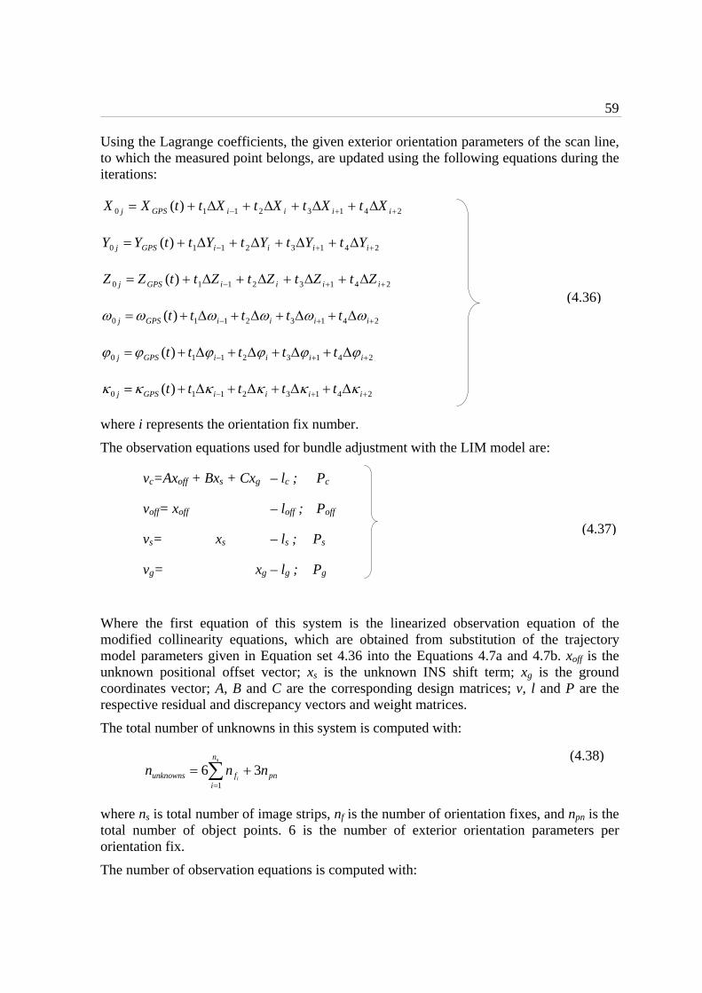
59

Using the Lagrange coefficients, the given exterior orientation parameters of the scan line, to which the measured point belongs, are updated using the following equations during the iterations:

24132110 )( iiiiGPSj XtXtXtXttXX

24132110 )( iiiiGPSj YtYtYtYttYY

24132110 )( iiiiGPSj ZtZtZtZttZZ

24132110 )( iiiiGPSj ttttt

24132110 )( iiiiGPSj ttttt

24132110 )( iiiiGPSj ttttt

where i represents the orientation fix number.

The observation equations used for bundle adjustment with the LIM model are:

vc=Axoff + Bxs + Cxg – lc ; Pc

voff= xoff – loff ; Poff

vs= xs – ls ; Ps

vg= xg – lg ; Pg

Where the first equation of this system is the linearized observation equation of the modified collinearity equations, which are obtained from substitution of the trajectory model parameters given in Equation set 4.36 into the Equations 4.7a and 4.7b. xoff is the unknown positional offset vector; xs is the unknown INS shift term; xg is the ground coordinates vector; A, B and C are the corresponding design matrices; v, l and P are the respective residual and discrepancy vectors and weight matrices.

The total number of unknowns in this system is computed with:

pn

n

ifunknowns nnn

s

i36

1

where ns is total number of image strips, nf is the number of orientation fixes, and npn is the total number of object points. 6 is the number of exterior orientation parameters per orientation fix.

The number of observation equations is computed with:

(4.37)

(4.38)

(4.36)

60

gcpcsraysnsobservatio nnnn 32

where nrays is the number of measured image points (rays), ngcp is the number of full ground control points in the adjustment, and ncs is the number of observation equations used as constraints for the given EO parameters at each orientation fix. ncs is computed using:

s

i

n

ifcs nn

1

6

where ns is total number of image strips and nf is the number of orientation fixes.

The minimum number of orientation fixes is defined as 4 in the TLS-LAB software, due to the number of Lagrange coefficients used in the model (Eq. 4.35).

Figure 4.10 demonstrates the number of unknown and known parameters in the adjustment, when LIM is applied with 4 orientation fixes, without self-calibration, and 3 control and 3 tie points.

Figure 4.10. A demonstration of the number of known and unknown parameters in the LIM using 4 orientation fixes, 3 GCPs, and 3 tie points. The triangles and the solid circles represent the GCPs and the tie points, respectively. The unknown and known parameters are marked with bold and italic characters, respectively.

Computation of the minimum number of image rays

The minimum number of image rays between any two fixes is computed separately for the adjustment models with and without self-calibration. Figure 4.11 represents the relation between the adjustment redundancy and the number of points (GCP, check and tie) between any two orientation fixes, orientation fix number, and the number of GCPs, according to the following assumptions:

- All GCPs are full control points

- All points are evenly distributed between the fixes over the whole strip

(4.39)

(4.40)

6EO 6EO 6EO 6EO

3(x,y) 1(X,Y,Z) 1(X,Y,Z)

3(x,y) 1(X,Y,Z)

12 unknowns & 12 knowns

in total

18 unknowns & 15 knowns

in total

12 unknowns & 18 knowns

in total

Strip trajectory

Ori. fix 1 Ori. fix 2 Ori. fix 3 Ori. fix 4

3(x,y) 1(X,Y,Z) 1(X,Y,Z)

3(x,y) 1(X,Y,Z) 1(X,Y,Z)

3(x,y) 1(X,Y,Z)

3(x,y) 1(X,Y,Z)

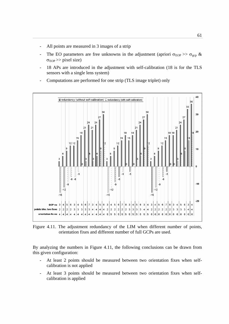
61

- All points are measured in 3 images of a strip

- The EO parameters are free unknowns in the adjustment (apriori EOP >> gcp & EOP >> pixel size)

- 18 APs are introduced in the adjustment with self-calibration (18 is for the TLS sensors with a single lens system)

- Computations are performed for one strip (TLS image triplet) only

Figure 4.11. The adjustment redundancy of the LIM when different number of points, orientation fixes and different number of full GCPs are used.

By analyzing the numbers in Figure 4.11, the following conclusions can be drawn from this given configuration:

- At least 2 points should be measured between two orientation fixes when self-calibration is not applied

- At least 3 points should be measured between two orientation fixes when self-calibration is applied

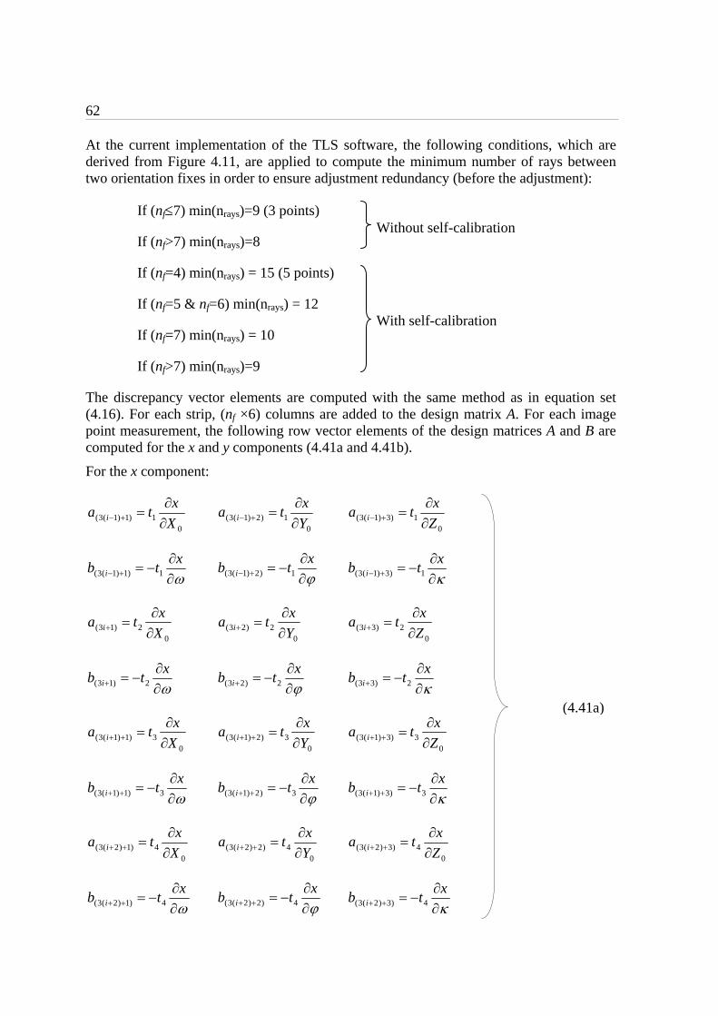
62

At the current implementation of the TLS software, the following conditions, which are derived from Figure 4.11, are applied to compute the minimum number of rays between two orientation fixes in order to ensure adjustment redundancy (before the adjustment):

If (nf7) min(nrays)=9 (3 points)

If (nf>7) min(nrays)=8

If (nf=4) min(nrays) = 15 (5 points)

If (nf=5 & nf=6) min(nrays) = 12

If (nf=7) min(nrays) = 10

If (nf>7) min(nrays)=9

The discrepancy vector elements are computed with the same method as in equation set (4.16). For each strip, (nf ×6) columns are added to the design matrix A. For each image point measurement, the following row vector elements of the design matrices A and B are computed for the x and y components (4.41a and 4.41b).

For the x component:

01)1)1(3( X

xta i

01)2)1(3( Y

xta i

0

1)3)1(3( Z

xta i

x

tb i 1)1)1(3(

x

tb i 1)2)1(3(

x

tb i 1)3)1(3(

02)13( X

xta i

02)23( Y

xta i

02)33( Z

xta i

x

tb i 2)13(

x

tb i 2)23(

x

tb i 2)33(

03)1)1(3( X

xta i

03)2)1(3( Y

xta i

03)3)1(3( Z

xta i

x

tb i 3)1)1(3(

x

tb i 3)2)1(3(

x

tb i 3)3)1(3(

04)1)2(3( X

xta i

04)2)2(3( Y

xta i

04)3)2(3( Z

xta i

x

tb i 4)1)2(3(

x

tb i 4)2)2(3(

x

tb i 4)3)2(3(

(4.41a)

Without self-calibration

With self-calibration

63

For the y component:

01)1)1(3( X

yta i

01)2)1(3( Y

yta i

0

1)3)1(3( Z

yta i

y

tb i 1)1)1(3(

y

tb i 1)2)1(3(

y

tb i 1)3)1(3(

02)13( X

yta i

02)23( Y

yta i

02)33( Z

yta i

y

tb i 2)13(

y

tb i 2)23(

y

tb i 2)33(

03)1)1(3( X

yta i

03)2)1(3( Y

yta i

03)3)1(3( Z

yta i

y

tb i 3)1)1(3(

y

tb i 3)2)1(3(

y

tb i 3)3)1(3(

04)1)2(3( X

yta i

04)2)2(3( Y

yta i

04)3)2(3( Z

yta i

y

tb i 4)1)2(3(

y

tb i 4)2)2(3(

y

tb i 4)3)2(3(

The derivatives used for these coefficients are computed with the Equations (4.18) and (4.19). The design matrix C is generated using the same formula as in the DGR model. When large position and attitude offset errors are expected in the trajectory, performing the adjustment with the DGR model before the LIM to correct these offset errors increases the adjustment stability. This approach is not necessarily used for PPM, since the problem can be solved by giving appropriate weights to the polynomial parameters.

The structural characteristic of the design matrices A, B, and C of Eq. 4.37 and the discrepancy matrix are represented in Figure 4.12. The resulting normal equations matrix (N = Qxx

-1 in Eq. A.14) and the solution vector ( x in Eq. A.6) is demonstrated in Figure 4.13. The matrices demonstrated in both Figures are formed for one TLS image strip, where three images share the same set EO data, and 6 orientation fixes.

(4.41b)

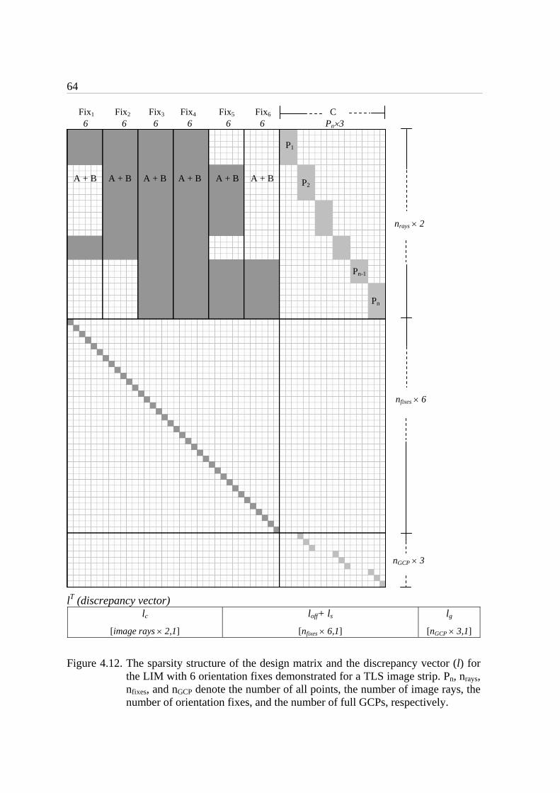
64

Fix1 Fix2 Fix3 Fix4 Fix5 Fix6 C 6 6 6 6 6 6 Pn3

lT (discrepancy vector) lc

[image rays 2,1]

loff+ ls

[nfixes 6,1]

lg

[nGCP 3,1]

Figure 4.12. The sparsity structure of the design matrix and the discrepancy vector (l) for the LIM with 6 orientation fixes demonstrated for a TLS image strip. Pn, nrays, nfixes, and nGCP denote the number of all points, the number of image rays, the number of orientation fixes, and the number of full GCPs, respectively.

A + B A + B

P1

P2

Pn-1

Pn

A + B A + B A + B A + B

nrays 2

nfixes 6

nGCP 3

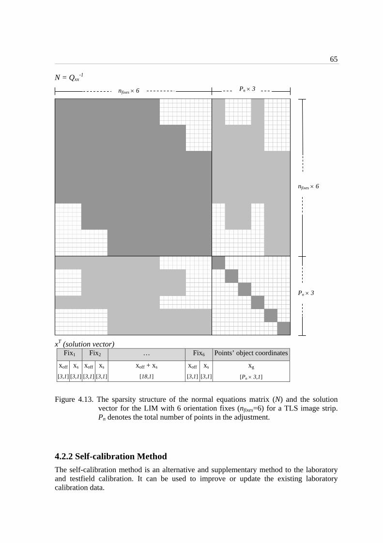
65

N = Qxx-1

xT (solution vector) Fix1 Fix2 … Fix6 Points’ object coordinates

xoff

[3,1]

xs

[3,1]

xoff

[3,1]

xs

[3,1]

xoff + xs

[18,1]

xoff

[3,1]

xs

[3,1]

xg

[Pn 3,1]

Figure 4.13. The sparsity structure of the normal equations matrix (N) and the solution vector for the LIM with 6 orientation fixes (nfixes=6) for a TLS image strip. Pn denotes the total number of points in the adjustment.

4.2.2 Self-calibration Method

The self-calibration method is an alternative and supplementary method to the laboratory and testfield calibration. It can be used to improve or update the existing laboratory calibration data.

nfixes 6

Pn 3

nfixes 6 Pn 3

66

Additional parameters are defined and applied to the image coordinates to correct for potential systematic errors of the sensor and other system components (e.g. atmospheric effects). The right-hand sides of the collinearity equations (A.21a and A.21b in Appendix) are expanded with additional parameter functions xij , yij:

xij = ijpj

z

xj xx

f

fc

yij = ijpj

z

yj yy

f

fc

The terms xij and yij can be understood as corrections to the image coordinates xij and yij in order to reduce the physical reality of the sensor geometry to the perspective model. They are usually meaningful functions of image coordinates.

4.2.2.1 Functional Model of the Additional Parameters for the Airborne TLS Sensors

A graphical representation of the CCD line structure and image coordinate system of a TLS system is given in Figure 4.14.

Figure 4.14. CCD line structure of TLS. (x,y) denote the image coordinate system. Ob, On, and Of denote the CCD line centers for backward, nadir and forward images. b, n and f are the inclination angles with y axis for each CCD line. PP represents the principal point of the camera lens.

(4.42a)

(4.42b)

f

x (flight direction)

y

PP(xp,yp) Ob (x0b,y0b) Of (x0f,y0f)

On(x0n,y0n)

b

n

Backward CCD Line

Nadir CCD Line

Forward CCD Line

67

Additional parameters used for the self-calibration of TLS sensors are:

c: Systematic error in the focal length of the camera lens.

Lens Distortion Parameters: Radial symmetric lens distortion (k1, k2, k3) and decentering distortion (p1, p2) models of Brown (1971).

xp: Displacement of the CCD line center from the principal point (PP) of the camera lens, defined in the flight direction.

yp: Displacement of the CCD line center from the principal point (PP) of the camera lens, defined across the flight direction.

sy: Scale parameter, defined in the (y) direction.

: Systematic error of the inclination angle between the CCD line and the (y) axis of the camera coordinate system (Figure 4.14). The effect of on the y-coordinates can be neglected due to the small error magnitude.

The functional model for self-calibration of a TLS system with backward, nadir and forward images include a total of 18 APs and is formed as:

xi<b,n,f> = xp<b,n,f>-c

xx pi )( c + (xi-xp)ri2k1 + (xi-xp)ri

4k2 +(xi-xp)ri6k3

+ (ri2 +2(xi-xp)

2 )p1 +2(xi-xp) (yi-yp)p2 +

)y-(y pi <b,n,f>

yi<b,n,f> = yp<b,n,f>-c

yy pi )( c+(yi-yp)ri2k1 + (yi-yp)ri

4k2 +(yi-yp)ri6k3

+ (ri2 +2(yi-yp)

2 )p2 +2(xi-xp)(yi-yp)p1 – (yi-yp)sy<b,n,f>

where; xi, yi : image coordinates of each point,

xp, yp : image coordinates of the principal point

= 180/π

ri2 =(xi-xp)

2 +(yi-yp) 2

The CCD line bending parameter, which is explained in Chapter 3.2.4, is not introduced for the TLS sensor in order to prevent over-parameterization.

(4.43a)

(4.43b)

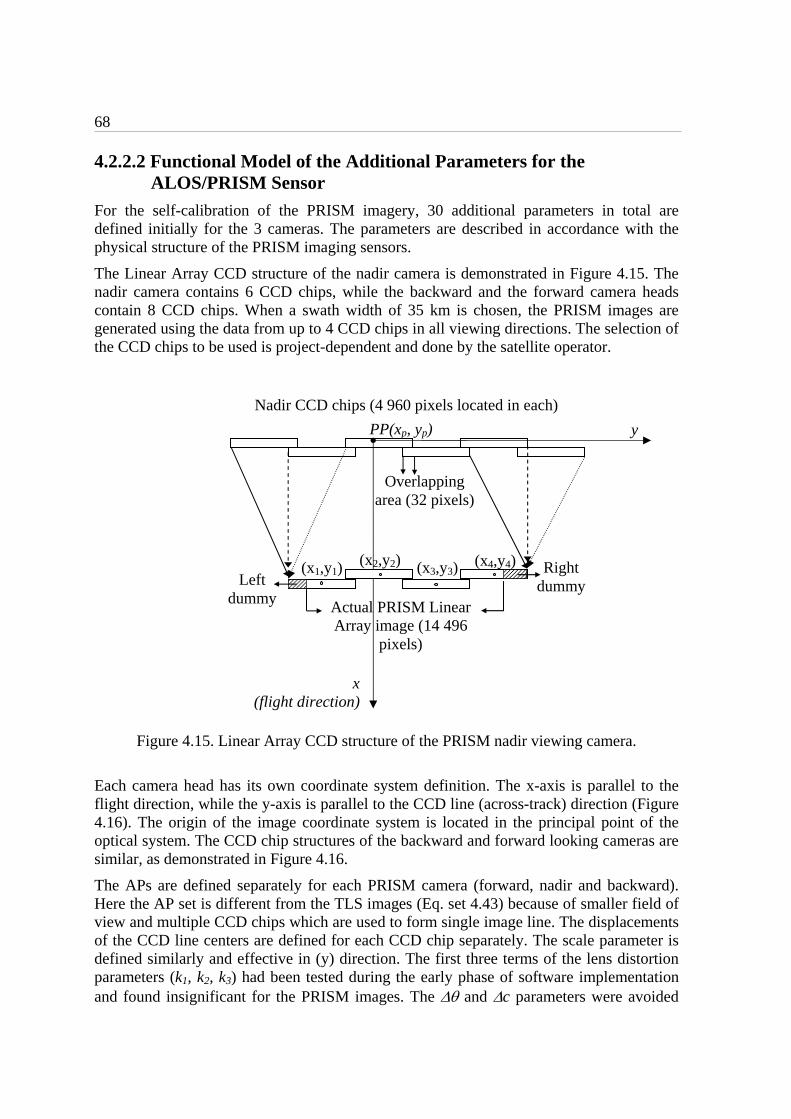
68

4.2.2.2 Functional Model of the Additional Parameters for the ALOS/PRISM Sensor

For the self-calibration of the PRISM imagery, 30 additional parameters in total are defined initially for the 3 cameras. The parameters are described in accordance with the physical structure of the PRISM imaging sensors.

The Linear Array CCD structure of the nadir camera is demonstrated in Figure 4.15. The nadir camera contains 6 CCD chips, while the backward and the forward camera heads contain 8 CCD chips. When a swath width of 35 km is chosen, the PRISM images are generated using the data from up to 4 CCD chips in all viewing directions. The selection of the CCD chips to be used is project-dependent and done by the satellite operator.

Figure 4.15. Linear Array CCD structure of the PRISM nadir viewing camera.

Each camera head has its own coordinate system definition. The x-axis is parallel to the flight direction, while the y-axis is parallel to the CCD line (across-track) direction (Figure 4.16). The origin of the image coordinate system is located in the principal point of the optical system. The CCD chip structures of the backward and forward looking cameras are similar, as demonstrated in Figure 4.16.

The APs are defined separately for each PRISM camera (forward, nadir and backward). Here the AP set is different from the TLS images (Eq. set 4.43) because of smaller field of view and multiple CCD chips which are used to form single image line. The displacements of the CCD line centers are defined for each CCD chip separately. The scale parameter is defined similarly and effective in (y) direction. The first three terms of the lens distortion parameters (k1, k2, k3) had been tested during the early phase of software implementation and found insignificant for the PRISM images. The and c parameters were avoided

y

x(flight direction)

PP(xp, yp)

Actual PRISM Linear Array image (14 496

pixels)

Left dummy

Right dummy

Nadir CCD chips (4 960 pixels located in each)

Overlapping area (32 pixels)

(x1,y1)(x2,y2) (x3,y3)

(x4,y4)

69

due to inevitable high correlation with the EO parameters () and Z0, respectively. In case of the aerial TLS images, this problem has not been considered, because of the multiple CCD lines, which are located on the focal plane and are sharing the same set of EO parameters.

On the other hand, the CCD line bending parameter has been introduced to correct the effect of potential non-linear (arc shaped) systematic deformation of the row of chips.

Figure 4.16. The backward and forward imaging lines contain 8 CCD chips. 32 pixels are located in the overlapping area. There is one coordinate system definition per camera (x: flight direction; y: CCD line direction). The camera principal point is the origin of the image coordinate system.

The AP set of each image includes:

- scale effect s in y direction (per image),

- CCD line bending b parameter (per image),

- 2 x 4 = 8 displacements of the centres of the CCD chips from the principal point (per image)

The terms xij and yij of Equations (4.42a) and (4.42b) include the APs used to model the systematic errors. The mathematical expressions of the correction terms xij and yij are:

xij = xnj + yijrij2bj

yij = ynj + yijsj

with

i = 1,…, m; m = number of points

j = 1,…, 3 number of cameras

(4.44a)

(4.44b)

y

x(flight direction)

PP(xp, yp)

Actual PRISM image (14 496 x 16 000 pixels)

(CCD chip coverage is project-variant)

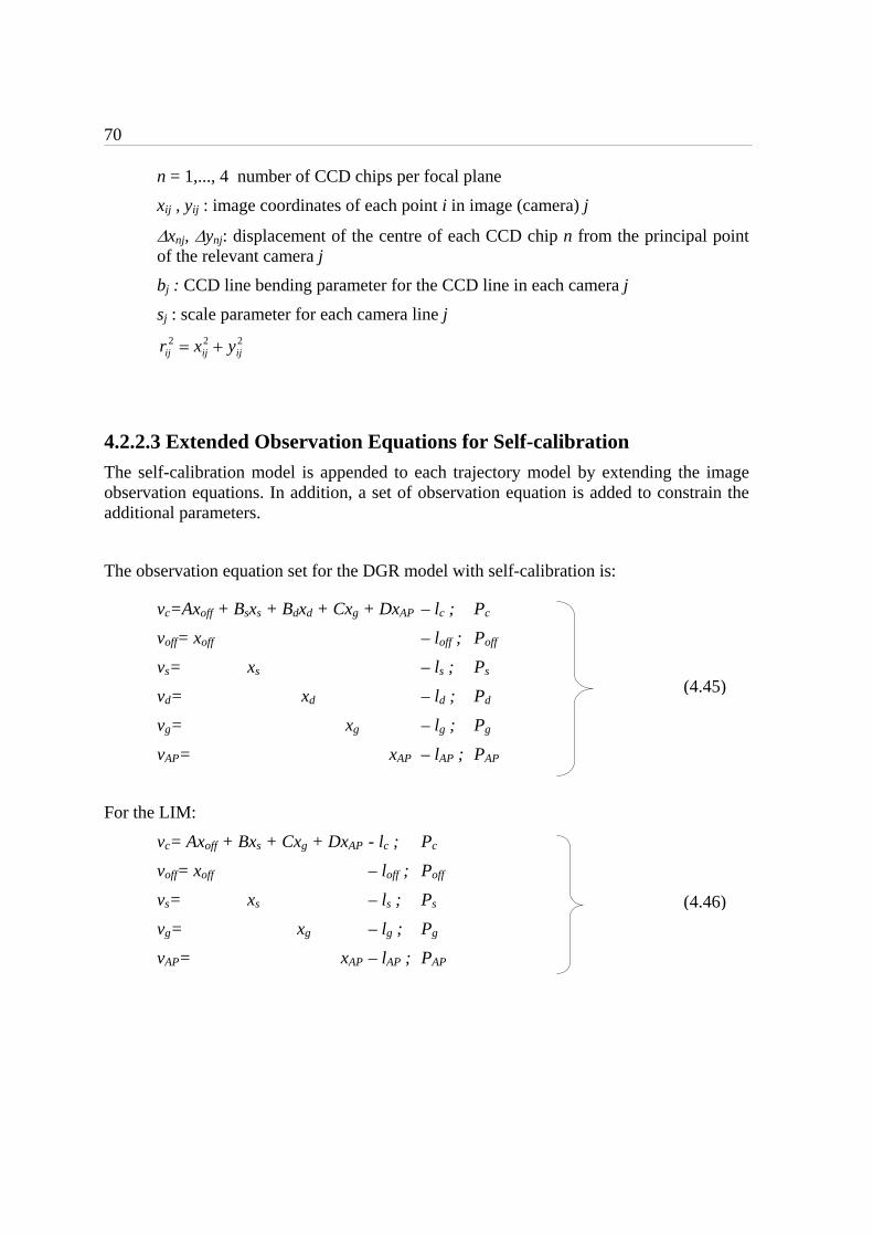
70

n = 1,..., 4 number of CCD chips per focal plane

xij , yij : image coordinates of each point i in image (camera) j

xnj, ynj: displacement of the centre of each CCD chip n from the principal point of the relevant camera j

bj : CCD line bending parameter for the CCD line in each camera j

sj : scale parameter for each camera line j 222ijijij yxr

4.2.2.3 Extended Observation Equations for Self-calibration

The self-calibration model is appended to each trajectory model by extending the image observation equations. In addition, a set of observation equation is added to constrain the additional parameters.

The observation equation set for the DGR model with self-calibration is:

vc=Axoff + Bsxs + Bdxd + Cxg + DxAP – lc ; Pc

voff= xoff – loff ; Poff

vs= xs – ls ; Ps

vd= xd – ld ; Pd

vg= xg – lg ; Pg

vAP= xAP – lAP ; PAP

For the LIM:

vc= Axoff + Bxs + Cxg + DxAP - lc ; Pc

voff= xoff – loff ; Poff

vs= xs – ls ; Ps

vg= xg – lg ; Pg

vAP= xAP – lAP ; PAP

(4.45)

(4.46)

71

For the PPM:

vc = Axpos + Bxatt + Cxg + DxAP – lc ; Pc

vpos= xpos – lpos; Ppos

vA2=A1xpos – lA1; PA1

vA3=A2xpos – lA2; PA2

vatt= xatt – latt; Patt

vB2= B1xatt – lB1; PB1

vB1= B2xatt – lB2; PB2

vg = xg – lg ; Pg

vAP= xAP – lAP ; PAP

Since the functional models of self-calibration (Equation sets 4.43 and 4.44) are already linear, linearization is not necessary. The elements of the design matrices D (d1, d2, …, dn ; n=18) in Equations (4.45 - 4.47) are computed according to the functional model. For the airborne TLS sensors, the Equations (4.48a and 4.48b) are extracted from the Equations (4.43a and 4.43b). Similarly, the Equations (4.49a and 4.49b) are extracted from the Equations (4.44a and 4.44b) for the ALOS/PRISM sensor.

For the TLS sensors, we get for the x components:

1pxd

c

xxd pi

c

2)(1

rxxd pik 4)(2

rxxd pik

6)(3

rxxd pik )(22

1 pip xxrd

))((22 pipip yyxxd pi yyd

(4.48a)

(4.47)

72

For the TLS sensors, we get for the y components:

1pyd

c

yyd pi

c

2)(1

ryyd pik 4)(2

ryyd pik

6)(3

ryyd pik ))((21 pipip yyxxd

)(22

2 pip yyrd )( pis yydy

For the ALOS/PRISM sensor, we get for the x components:

1njxd 2

ijijb rydj

For the ALOS/PRISM sensor, we get for the y components:

1njyd ijs yd

j

4.2.2.4 Determinability Analysis for the Self-Calibration Parameters

The aim of self-calibration for this work is to determine the optimal set of APs for optimal estimation of the object space coordinates of the measured image points. The adjustment procedure starts with the full parameter set and eliminates undeterminable parameters automatically in an iterative approach. The APs are introduced as free unknowns into the system. The major problem for parameter elimination is to find robust criteria for rejection of undeterminable parameters. A stepwise parameter elimination algorithm proposed by Gruen (1985a) is used here. The algorithm includes:

i. Determinability check by analyzing the diagonal elements of the factorized normal matrix during Cholesky decomposition. If an element falls below a pivot value, the parameter is excluded from the system by replacing this element with a large number.

ii. Correlation analysis between the APs and the EO parameters, and also between the APs and the points’ object space coordinates. Elements of the correlation coefficients matrix are computed using:

jjii

ijij

qq

qr

where qij, qii, and qjj are corresponding elements of the Qxx covariance matrix.

(4.48b)

(4.50)

(4.49a)

(4.49b)

73

iii. Analysis of the negative effect of each AP on the object space coordinates of the points by using the trace check algorithm of the covariance matrix. The effect of each AP is computed with:

pn

i

n

jjjij

pnAP qr

n 1

220

2 1

where, 0 is the a priori standard deviation of the unit weight, npn is the total

number of points in the adjustment, rij is the correlation coefficient between the AP i and corresponding coordinate of the point j, and qjj is the corresponding element of the Qxx covariance matrix. The

iAP values of each AP i are computed for the

X,Y,Z coordinate components separately and compared with a critical value. The critical value is chosen as a ratio of the image GSD.

iv. Statistical significance tests under Student’s t distribution for the individual analysis of the APs; and under Fisher (F) distribution for the analysis of sub-sets of APs are applied. Six groups of APs, which consist of (xpb, , xpn ,xpf), (ypb,, ypn ,ypf), (syb, syn, syf), (b ,n, f), (k1, k2, k3), (p1, p2), are tested with the F-distribution due to strong correlations between the parameters of the same group.

Student’s t distribution values are computed for each additional parameter using:

ti = ii

i

q

x

0ˆ

ˆ

where ti is Student’s t distribution value, ix is the estimated AP value, 0 is the a

posteriori standard deviation of unit weight, qii is the corresponding diagonal element of covariance matrix of unknowns. The distribution value is compared with a threshold value t, which is chosen by the user according to the significance level required. If ti<t, then the parameter is considered as insignificant in the bundle system.

),...,,(ˆ 21 kT xxxx parameters are tested in every sub-set of APs, and the statistical

variable of F distribution for each group is obtained as follows:

20

1ˆˆ

ˆ

ˆˆ

kxQx

F xxT

where x is the estimated parameter vector in the bundle adjustment, xxQ ˆˆ is the

corresponding part of the covariance matrix, k is the number of APs in the group, and 0 is the a posteriori standard deviation of the unit weight. The obtained F

value is compared with a threshold value, computed with an assumed significance level . When F<F, then the AP group is considered as insignificant.

(4.52)

(4.51)

(4.53)

74

4.2.3 Weighting Scheme of the Bundle Adjustment

The weighting scheme is of high importance for the triangulation of Linear Array Imagery. The unknown parameters of the bundle adjustment, in particular the trajectory unknowns, are usually highly correlated. In order to ensure parameter determinability under the weakening correlation pattern, the given EO parameters measured by GPS and INS/star tracker systems, shall be introduced as weighted observations. The weighting scheme plays a significant role in the adjustment accuracy.

The weight of an observation is computed using a priori standard deviation value according to the Equation A.8. Here, the standard deviation of the unit weight is always chosen as equal to a priori standard deviation of image measurements (0 = img). Selection of appropriate a priori standard deviations of the adjustment observations, including the constraint equations, is a crucial procedure for optimal estimation. The main principles followed here for a priori standard deviation selection are:

For trajectory unknowns, in principle the standard deviations provided by the sensor developer or data provider are taken into account. However, these values do not always represent the reality, due to the influences of operational and processing aspects which cause improvement or deterioration of the data quality. The trajectory data might be improved in a post-processing e.g. with Kalman Filtering, or may suffer from different types of errors, such as sensor relative alignment errors, lack of appropriate post-processing, etc. Therefore, the instrument precision values might be questionable and after the triangulation, the solution vector and the adjustment accuracy should be analyzed carefully in order to detect any anomaly caused by the weighting scheme.

For each trajectory model, different approaches are used to introduce the a priori standard deviations of the given EO data. In case of the DGR model, the a priori standard deviations of the position and attitude offset parameters (Xoff, Yoff, Xoff, o, o, o) are selected according to the principles above. The a priori standard deviations of attitude drift parameters (1, 1, 1) should represent the error budget of the INS/Star tracker instrument within a certain time interval. The standard deviation value used to compute the respective weight should reflect the total drift error for the entire image strip.

In case of the PPM, the Ppos and Patt matrices of the Eq. 4.26 are formed to introduce the quality of given trajectory data into the adjustment, whereas the PA1, PA2, PB1, PB2 are formed to ensure data continuity between neighboring segments. The unknown parameters of each polynomial segment (Eq. 4.22) are introduced individually in the Ppos and Patt matrices by forming 18 observation equations. The zero order parameters reflect the offset errors expected for the whole trajectory. The a priori standard deviations of the first and second order parameters should be in accordance with the expected maximum error values for an entire segment. The weight coefficients of the continuity constraints should be relatively high, representing the allowed differences between the position and attitude values of the two neighboring image lines located at the segment borders.

75

In case of the LIM, the Poff and Ps matrices (Eq. 4.37) are used for stochastic modeling of the trajectory unknowns. For each orientation fix, 3 position and 3 attitude offset parameters are estimated. The a priori standard deviations of these parameters represent the maximum errors to be estimated at an orientation fix. In comparison to the DGR and the PPM, the control of the adjustment with the stochastic model in LIM is considerably weaker due to large number of orientation parameters and fewer constraints. If a large number of orientation fixes is used in an image strip, a large number of control points or highly accurate trajectory data is required for precise modeling.

As a supplementary technique, if the given trajectory data contains large position and attitude offset errors, it is recommended to use the DGR prior to the LIM to model those errors. In a similar situation, the PPM can be run with one segment definition and low weights on the zero order parameters. After this adjustment, the trajectory shall be corrected. As a second step, the PPM can be run with multiple segments and with relatively higher weights on the zero order parameters. If the accuracy achieved in the first step is sufficient, the second step may not be necessary.

For image measurements, depending on the image quality and measurement accuracy, 0.3-0.5 pixels are usually taken as a priori standard deviation. The values can be judged by the operator, who performs the image measurements.

In principle, the additional parameters are introduced as free unknowns in the beginning of the adjustment. In practice, it is carried out by introducing very high a priori standard deviations (e.g. APi = 10 mm, etc.). In the parameter elimination procedure, undeterminable parameters are removed from the system by introducing very low standard deviation value to the corresponding parameter (e.g. APi = 0.000001 mm, etc.).

For the ground control points, the a priori standard deviations come from the ground data collection accuracy. The measurement accuracy varies with the measurement method. When a static GPS measurement method is used, the accuracy is usually better than 5 cm.

4.2.4 Accuracy Assessment of the Bundle Adjustment

The internal accuracy is expressed in terms of theoretical accuracy (precision) parameters. The theoretical sigma values (standard deviations) can be obtained from the analysis of the covariance matrix after the bundle adjustment or by using empirical accuracy values. The covariance matrix Kxx (Eq. A.12 in Appendix) is defined as a measure of precision of the solution x in the bundle block adjustment (Gruen, 1982).

Parameters used for internal quality control of the system are:

A posteriori standard deviation of unit weight (sigma naught):

76

un

PvvT

0

where, v is the residual vector, P is the weight matrix, n is the number of observations, and u is the number of unknowns. Equation (4.54) is analogous to the Equation (A.10) in Appendix.

Standard deviations of object space coordinates:

In the least squares adjustment procedure, the a posteriori sigma naught value and the elements of the covariance matrix Kxx (Eq. A.12 and Eq. A14 ) are used to compute the individual standard deviations of the object points.

iii XXX q0ˆˆ iii YYY q0ˆˆ

iii ZZZ q0ˆˆ

where ii XXq ,

iiYYq , iiZZq , are diagonal elements of the inverse of the normal equation

matrix at the position of the corresponding unknown.

As described by Gruen (1982), the means of the variances of the adjusted ground point coordinates are used as theoretical precision measures. The mean standard deviations for the point set are computed via the law of error propagation:

X

n

iX

X n

X

i 1

2ˆˆ

Y

n

iY

Y n

Y

i 1

2ˆˆ

Z

n

iZ

Z n

Z

i 1

2ˆˆ

with nX, nY, nZ number of point coordinates used for the computation, and iX ,

iY , and iZ are the standard deviations of the X,Y,Z coordinates obtained from the

covariance matrix. These parameters are computed and evaluated separately for control, check and tie points.

The absolute (external) accuracy is evaluated by using reference data. The differences between the given and estimated coordinates of check points (CP) are calculated to obtain the residuals. Check points are a subset of GCPs that are not used as control point in the adjustment procedure. The residuals of the CPs in object space are computed using:

riii XXX ˆˆ

riii YYY ˆˆ

riii ZZZ ˆˆ

(4.54)

(4.55)

(4.56)

(4.57)

77

where iX , iY iZ are the estimated ground coordinates of a CP (i), and riX , r

iY riZ are the

given coordinates.

A common representation of absolute accuracy of georeferencing is the root-mean-square error (RMSE) value. The RMSE is computed from the ground residuals of CPs using the following formulae:

X

n

ii

X n

XX

1

2ˆ

Y

n

ii

Y n

YY

1

2ˆ

Z

n

ii

Z n

ZZ

1

2ˆ

Where nX, nY, nZ are the numbers of CP coordinates; and iX , iY , iZ are the object

residuals computed by using the Equation set (4.57).

A large difference between the RMSE and the theoretical values is an indication of remaining systematic errors in the dataset.

The absolute maximum of the residuals in a CP set is an important measure of the quality of the point set and the georeferencing method.

The theoretical and the empirical accuracies in X and Y axes are often expressed with one parameter, and called “planimetric accuracy”. The formulations of the planimetric standard deviation and the planimetric RMSE are as follows:

2

ˆˆˆ

22

ii YXXY

2

ˆˆˆ

22

ii YXXY

The arithmetic mean values are often calculated and used to evaluate biases in the residuals:

Xn

ii

xX X

nmean

1

ˆ1

Yn

ii

YY Y

nmean

1

ˆ1

Zn

ii

ZZ Z

nmean

1

ˆ1

where nX, nY, nZ are number of CP coordinates; and iX , iY , iZ are the object

residuals computed in Equation set (4.57).

In an unbiased dataset, the arithmetic mean value should be close to zero.

The empirical standard deviations of a point set can be computed from the analysis of residuals by:

(4.58)

(4.59)

(4.60)

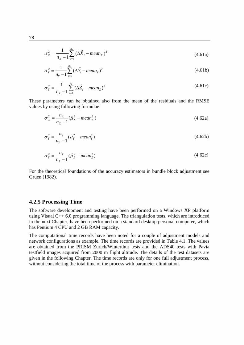
78

Xn

iXi

XX meanX

n 1

22 )ˆ(1

1

Yn

iYi

YY meanY

n 1

22 )ˆ(1

1

Zn

iZi

ZZ meanZ

n 1

22 )ˆ(1

1

These parameters can be obtained also from the mean of the residuals and the RMSE values by using following formulae:

)ˆ(1

222XX

X

XX mean

n

n

)ˆ(1

222YY

Y

YY mean

n

n

)ˆ(1

222ZZ

Z

ZZ mean

n

n

For the theoretical foundations of the accuracy estimators in bundle block adjustment see Gruen (1982).

4.2.5 Processing Time

The software development and testing have been performed on a Windows XP platform using Visual C++ 6.0 programming language. The triangulation tests, which are introduced in the next Chapter, have been performed on a standard desktop personal computer, which has Pentium 4 CPU and 2 GB RAM capacity.

The computational time records have been noted for a couple of adjustment models and network configurations as example. The time records are provided in Table 4.1. The values are obtained from the PRISM Zurich/Winterthur tests and the ADS40 tests with Pavia testfield images acquired from 2000 m flight altitude. The details of the test datasets are given in the following Chapter. The time records are only for one full adjustment process, without considering the total time of the process with parameter elimination.

(4.61a)

(4.61b)

(4.61c)

(4.62a)

(4.62b)

(4.62c)

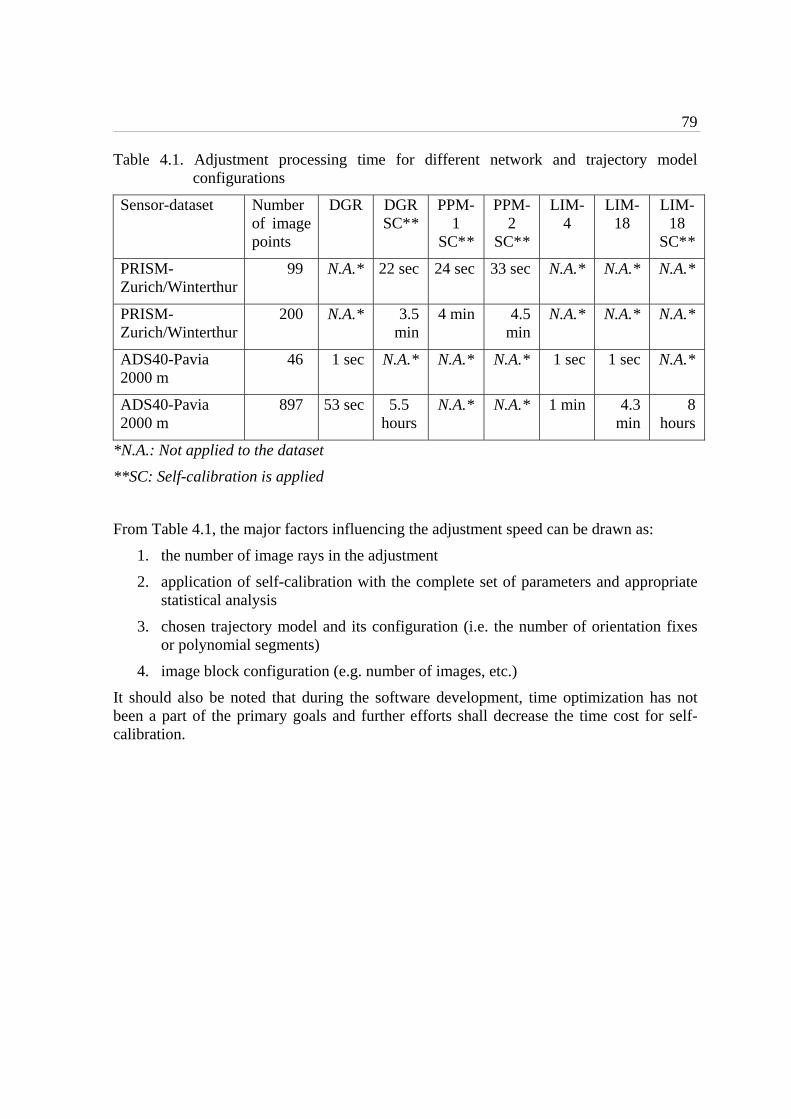
79

Table 4.1. Adjustment processing time for different network and trajectory model configurations

Sensor-dataset Number of image points

DGR DGR SC**

PPM-1

SC**

PPM-2

SC**

LIM-4

LIM-18

LIM-18

SC**

PRISM-Zurich/Winterthur

99 N.A.* 22 sec 24 sec 33 sec N.A.* N.A.* N.A.*

PRISM-Zurich/Winterthur

200 N.A.* 3.5 min

4 min 4.5 min

N.A.* N.A.* N.A.*

ADS40-Pavia 2000 m

46 1 sec N.A.* N.A.* N.A.* 1 sec 1 sec N.A.*

ADS40-Pavia 2000 m

897 53 sec 5.5 hours

N.A.* N.A.* 1 min 4.3 min

8 hours

*N.A.: Not applied to the dataset

**SC: Self-calibration is applied

From Table 4.1, the major factors influencing the adjustment speed can be drawn as:

1. the number of image rays in the adjustment

2. application of self-calibration with the complete set of parameters and appropriate statistical analysis

3. chosen trajectory model and its configuration (i.e. the number of orientation fixes or polynomial segments)

4. image block configuration (e.g. number of images, etc.)

It should also be noted that during the software development, time optimization has not been a part of the primary goals and further efforts shall decrease the time cost for self-calibration.

80

5

APPLICATIONS

The methodologies, which are proposed in Chapter 4 for geometric processing and validation of aerial and high-resolution satellite Linear Array CCD sensors, are applied to imagery of three different sensors. The STARIMAGER sensor of former Starlabo Corp., Japan, and the ADS40 sensor of the Leica Geosystems, Heerbrugg, Switzerland are the aerial Linear Array CCD sensors, which are operating with the Three-Line-Scanner principle. Applications of the proposed methods to the satellite Linear Array CCD sensor are realized using the imagery of the PRISM sensor, which operates onboard of the Japanese ALOS satellite. The images of all sensors are acquired over a number of specially designed testfields.

As a common procedure, Baarda’s data snooping algorithm (Eq. A.17) has been applied to all datasets before starting comprehensive testing, in order to eliminate blunder measurements from the point sets. This is a critical issue especially for large point sets, such as in ADS40 and STARIMAGER cases, where a great number of tie points were collected in automatic or semi-automatic fashion to provide sufficient flexibility with the LIM (i.e. selection of number of orientation fixes). The algorithm has worked successfully and the test datasets were free of gross errors.

This chapter is subdivided in three main subsections, one per sensor. The sensor descriptions and their applications to the testfields are given in the respective sections. Brief discussions on the results are provided for each sensor.

5.1 The STARIMAGER (TLS) Sensor

The STARIMAGER sensor was designed in the year 2000 by the Starlabo Corporation, Tokyo jointly with the Institute of Industrial Science, University of Tokyo. The system was originally called Three-Line-Scanner (TLS). The TLS system was initially designed to

82

record line features (roads, rivers, railways, power-lines, etc) only, but later tests also revealed the suitability for general mapping and GIS-related applications (Murai and Matsumoto, 2000). Starlabo Corporation has presented four different configurations of STARIMAGER cameras, namely SI-100, SI-250, SI-290, and SI-290N, with various numbers of CCD lines and pixels in each. The Starlabo Corporation has been discontinued and the system has passed to some of the shareholders of the company. The STARIMAGER is still in operation in Japan and used for airborne surveying and mapping applications.

The STARIMAGER systems are composed of eight major subsystems (imaging, data pre- and post-processing, trajectory data recording, data storage systems, etc.), which are discussed in Chen et al. (2003). The imaging system typically has three major subassemblies: stabilizer, INS, and the TLS. The TLS system produces seamless high-resolution images (5 - 10 cm footprint on the ground) in three viewing directions (forward, nadir and backward). The camera system is equipped with a high quality stabilizer. The stabilizer with five gimbals absorbs the vibrations of the aircraft movement and produces images with much less jitter than caused by an uncompensated platform movement.

The first design of the STARIMAGER system, called SI-100, consists of 3 Linear Array CCDs located on the focal plate of a single lens. Each line includes 12 000 CCD detectors with a size of 7 µm. In the later configurations (i.e. SI-250, SI-290, and SI-290N) 10 Linear Array CCDs having 14 400 pixels were used.

Two image datasets acquired over the Yoriichio Testfield, Japan with the SI-100 and SI-290 are processed in this study. The results of the SI-290 dataset were published in Kocaman (2005). The SI-100 dataset was analyzed in Kocaman et al. (2006). More details on the results are presented in the following sections. The sensor and dataset descriptions are provided accordingly.

5.1.1 Applications over the Yoriichio Testfield, Japan

5.1.1.1 SI-290 Dataset

The main system specifications of the SI290 sensor are given in Table 5.1. The focal distance of the SI-290 camera lens system is 93 mm, and the stereo angles are 15, 23, and 38, between forward and nadir, nadir and backward, and forward and backward, respectively. Each line sensor consists of 14 400 CCD pixels with 5 m spacing, and acquires 500 line images per second (2 msec acquisition interval), recorded with a controlling and recording device installed in the aircraft. A GPS antenna acquires the camera position signal at 5 Hz and the IMU on the top of the TLS camera acquires the camera attitude signal at 500 Hz. A Trimble MS750 serves as Rover GPS and collects L1/L2 kinematic data at 5 Hz and another Trimble MS750 serves as Base GPS on the ground. The stabilizer has a vibration-absorbing spring and 5 gimbals, absorbing the fluctuations of the aircraft, and keeps the optical axis direction of the TLS camera stable within a single pixel of the line sensor. The TLS camera and stabilizer are controlled by the electronic devices in the aircraft cabin, which record images, position and attitude data

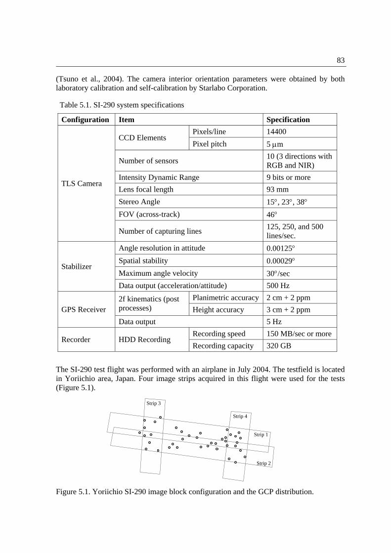
83

(Tsuno et al., 2004). The camera interior orientation parameters were obtained by both laboratory calibration and self-calibration by Starlabo Corporation.

Table 5.1. SI-290 system specifications

Configuration Item Specification

Pixels/line 14400 CCD Elements

Pixel pitch 5 m

Number of sensors 10 (3 directions with RGB and NIR)

Intensity Dynamic Range 9 bits or more

Lens focal length 93 mm

Stereo Angle 15, 23, 38

FOV (across-track) 46

TLS Camera

Number of capturing lines 125, 250, and 500 lines/sec.

Angle resolution in attitude 0.00125

Spatial stability 0.00029

Maximum angle velocity 30/sec Stabilizer

Data output (acceleration/attitude) 500 Hz

Planimetric accuracy 2 cm + 2 ppm 2f kinematics (post processes) Height accuracy 3 cm + 2 ppm GPS Receiver

Data output 5 Hz

Recording speed 150 MB/sec or more Recorder HDD Recording

Recording capacity 320 GB

The SI-290 test flight was performed with an airplane in July 2004. The testfield is located in Yoriichio area, Japan. Four image strips acquired in this flight were used for the tests (Figure 5.1).

Figure 5.1. Yoriichio SI-290 image block configuration and the GCP distribution.

Strip 1

Strip 2

Strip 3

Strip 4

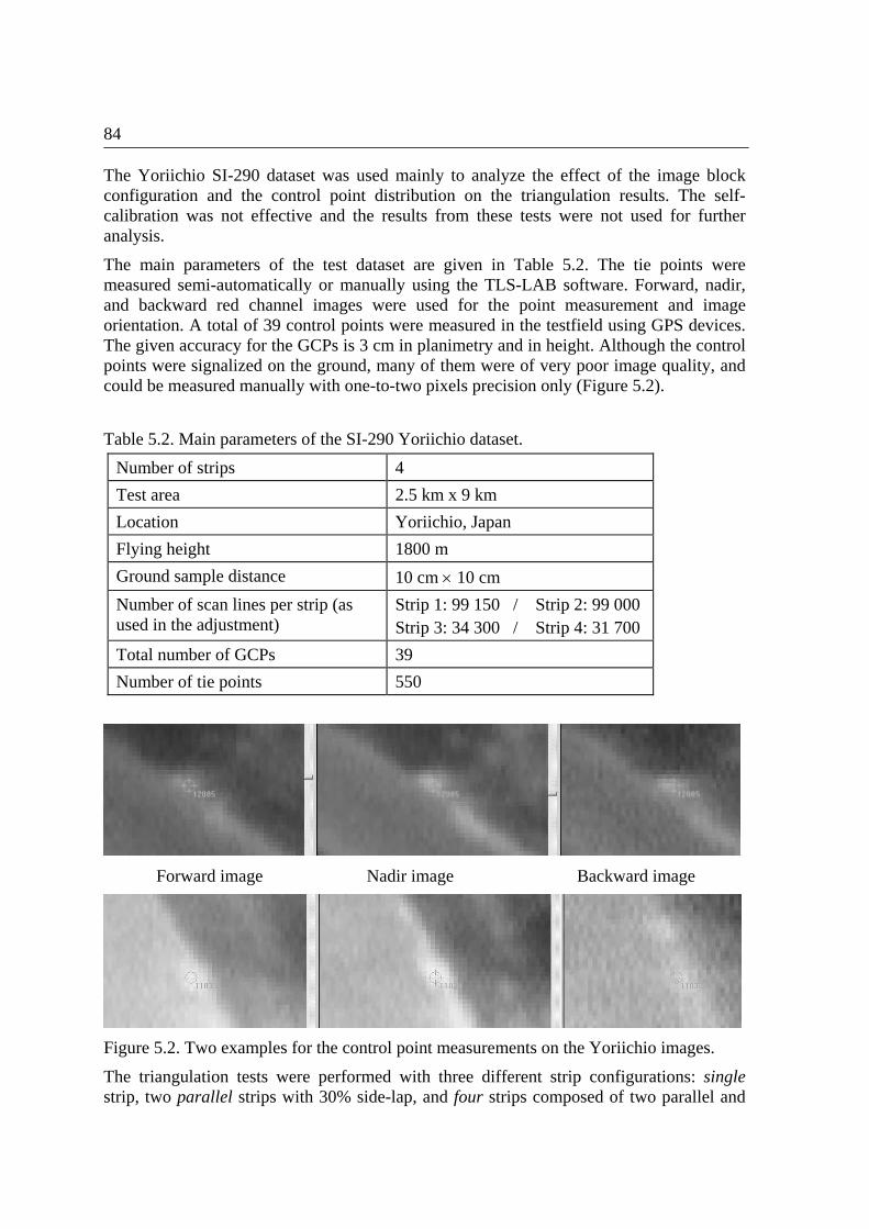
84

The Yoriichio SI-290 dataset was used mainly to analyze the effect of the image block configuration and the control point distribution on the triangulation results. The self-calibration was not effective and the results from these tests were not used for further analysis.

The main parameters of the test dataset are given in Table 5.2. The tie points were measured semi-automatically or manually using the TLS-LAB software. Forward, nadir, and backward red channel images were used for the point measurement and image orientation. A total of 39 control points were measured in the testfield using GPS devices. The given accuracy for the GCPs is 3 cm in planimetry and in height. Although the control points were signalized on the ground, many of them were of very poor image quality, and could be measured manually with one-to-two pixels precision only (Figure 5.2).

Table 5.2. Main parameters of the SI-290 Yoriichio dataset.

Number of strips 4

Test area 2.5 km x 9 km

Location Yoriichio, Japan

Flying height 1800 m

Ground sample distance 10 cm 10 cm

Number of scan lines per strip (as used in the adjustment)

Strip 1: 99 150 / Strip 2: 99 000 Strip 3: 34 300 / Strip 4: 31 700

Total number of GCPs 39

Number of tie points 550

Forward image Nadir image Backward image

Figure 5.2. Two examples for the control point measurements on the Yoriichio images.

The triangulation tests were performed with three different strip configurations: single strip, two parallel strips with 30% side-lap, and four strips composed of two parallel and

85

two cross strips. The strip-1, demonstrated in Figure 5.1, was used for single strip tests, while the strip-1 and strip-2 were used for the parallel strips tests.

For each configuration, various numbers of control points were used. In order to analyze the effect of control point distribution on the accuracy results, different sets of control points having the same number in total were tested for some cases. Each test was named with the number of control points used. If two tests were performed with the same number of control points having different distributions, then a second number was set as suffix to distinguish between tests. For example, T.3-1 and T.3-2 represent two different tests both performed with three control points but with different GCP distributions.

For each test, the GCPs, which were not used as control points, were used as check points. The image coordinates of the check points were used as observations together with the control and tie points in the bundle adjustment.

The tests were performed using the DGR model and the LIM with four different numbers of orientation fixes (5, 15, 30, and 45). The number of image lines between any two orientation fixes for the LIM are approximately:

5 orientation fixes: 25 000, 8 500, and 8 000 for the strips 1&2, strip 3, and strip 4 respectively

15 orientation fixes: 7 000 and 2 500 for the strips 1&2 and the strips 3 & 4 respectively

30 orientation fixes: 3 400, 2 000, 2 400 for the strips 1&2, strip 3, and strip 4 respectively

45 orientation fixes: 2250, 2000, and 2400 for the strips 1&2, strip 3, and strip 4 respectively

The given number of orientation fixes are nominal and defined by the user before the adjustment starts. The actual numbers are computed automatically by the software and limited according to the number of image observations available between the fixes. The details of the computational principles are given in Section 4.2.1.3.

The a priori standard deviations of the unknown parameters used to compute the weight coefficients matrices in the LIM and the DGR are given Table 5.3. Since the information of trajectory data quality was not available from the Starlabo Corp., the approximations for the a priori standard deviations were obtained from the DGR tests with all GCPs and very low weights on the EO parameters. The values are kept the same in all test configurations of the SI-290 dataset.

The a posteriori sigma naught ( 0 ) values obtained from the tests with different models

for all block configurations are demonstrated in Figure 5.3. Since the 0 values do not

vary with the number of control points used in the adjustment, only the values obtained from 4 GCP tests are presented in the graph. From the Figure 5.3 it can be clearly seen that the increase in the number of orientation fixes has a positive effect on the 0 .

86

Table 5.3. A priori standard deviations used for the unknown parameters of the SI-290 dataset.

Parameter Std. deviation () in DGR Std. deviation () in LIM*

Xoff, Yoff 20 m 2 m

Zoff 5 m 2 m

0, 0 0.2 0.1

0 3 0.1

1, 1, 1 0.2 Not applicable

GCP (X,Y,Z) 3 cm 3 cm

Image measurement Initial: 2 pixels

After 3rd iteration: 0 Initial: 0 obtained from the

DGR

After 3rd iteration: 0

* The DGR is run prior to the LIM in order to remove large position and attitude offsets from the system.

The triangulation results are presented in the following parts according to the image block configuration (single, parallel and cross-strip configurations).

Figure 5.3. A posteriori sigma naught values of the all block configurations obtained from the 4 GCP tests.

4.00

6.00

8.00

10.00

12.00

14.00

16.00

18.00

DGR LIM-5 LIM-15 LIM-30 LIM-45

mic

ron

s

Model

Single strip

2-strips

4-strips

87

Single Strip Results

22 GCPs and 273 tie points are measured in Strip-1 (Figure 5.1). The DGR results are given in Figure 5.4. The use of a higher number of GCPs improved the RMSE values significantly. However, the improvements in sigma values were not significant in this case. In comparison to T.4, T.6-1 has a better control distribution at the edges of the strip, that provides an important improvement in planimetric RMSE. From the results it can be said that the DGR model was not sufficient to model the systematic errors of the trajectories.

On the other hand, the LIM delivers better sigma and RMSE values than the DGR model (Figures 5.5 and 5.6). However, the single strip has poorer geometry than the multiple-cross strip block configuration and a greater number of control points were necessary to provide the system stability. Therefore, the number of orientation fixes should be chosen carefully in order to keep the system stable. The LIM-15 delivers better accuracy values than the LIM-45. In addition, when a small number of control points are used, a small number of orientation fixes should be preferred. In comparison to the DGR model results, the increase of the number of control points has a more significant effect on the LIM results. The GCP distribution is also more important when the LIM is used. When two different versions of the 3 and 6 GCP cases are compared, the results of DGR do not show large differences. However, the LIM delivers significantly different results when the different distributions are chosen for the same number of control points.

Figure 5.4. The DGR model results for the single strip with different numbers and

distributions of GCPs.

88

Figure 5.5. LIM results with 15 orientation fixes for the single strip with different numbers and distributions of GCPs.

Figure 5.6. LIM results with 45 orientation fixes for the single strip with different number and distribution of GCPs.

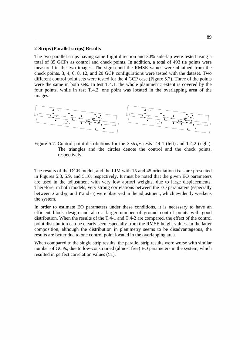
89

2-Strips (Parallel-strips) Results

The two parallel strips having same flight direction and 30% side-lap were tested using a total of 35 GCPs as control and check points. In addition, a total of 493 tie points were measured in the two images. The sigma and the RMSE values were obtained from the check points. 3, 4, 6, 8, 12, and 20 GCP configurations were tested with the dataset. Two different control point sets were tested for the 4 GCP case (Figure 5.7). Three of the points were the same in both sets. In test T.4.1. the whole planimetric extent is covered by the four points, while in test T.4.2. one point was located in the overlapping area of the images.

Figure 5.7. Control point distributions for the 2-strips tests T.4-1 (left) and T.4.2 (right). The triangles and the circles denote the control and the check points, respectively.

The results of the DGR model, and the LIM with 15 and 45 orientation fixes are presented in Figures 5.8, 5.9, and 5.10, respectively. It must be noted that the given EO parameters are used in the adjustment with very low apriori weights, due to large displacements. Therefore, in both models, very strong correlations between the EO paramaters (especially between X and , and Y and ) were observed in the adjustment, which evidently weakens the system.

In order to estimate EO parameters under these conditions, it is necessary to have an efficient block design and also a larger number of ground control points with good distribution. When the results of the T.4-1 and T.4-2 are compared, the effect of the control point distribution can be clearly seen especially from the RMSE height values. In the latter composition, although the distribution in planimetry seems to be disadvantageous, the results are better due to one control point located in the overlapping area.

When compared to the single strip results, the parallel strip results were worse with similar number of GCPs, due to low-constrained (almost free) EO parameters in the system, which resulted in perfect correlation values (1).

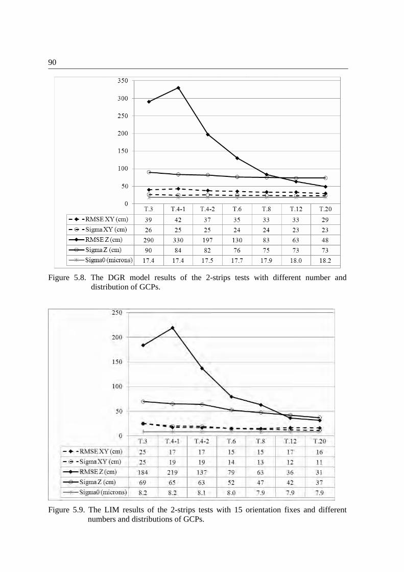
90

Figure 5.8. The DGR model results of the 2-strips tests with different number and distribution of GCPs.

Figure 5.9. The LIM results of the 2-strips tests with 15 orientation fixes and different numbers and distributions of GCPs.

91

Figure 5.10. The LIM results of 2-strips tests with 45 orientation fixes and different numbers and distributions of GCPs.

4-Strips Results

The 4-strips block is composed of two parallel and two cross strips. A total of 39 ground control points were used as control and check points for the adjustment. 553 tie points were distributed homogeneously in all four images. 3, 4, 6, 8, 12, and 20 control point distributions were tested to observe the number of control points on the results. Two different distributions of 3 and 6 GCP cases were tested. The two different distributions of the 3 GCP cases are given in Figure 5.11. In the T.3-1 case, the two points on the left side were selected to cover a larger planimetric extent of the area. In the T.3-2 distribution, the two GCPs on the left were measured in two strips.

Figure 5.11. Control point distribution for the 4-strips test T.3-1 (left) and T.3-2 (right).

92

The results of the DGR model and the LIM with 45 fixes are given in Table 5.4. For the DGR results, the difference in RMSE height between T.3-1 and T.3-2 was caused by the different distributions of the control points. However, comparing the LIM-45 results of these two distributions, it is not possible to prefer any of the distributions as they provided equal level of accuracies. With the DGR model, the main improvement from 3 to 20 control points was in height (Table 5.4, Figure 5.12). From 3 to 20 control points, the height RMSE values showed an improvement of 25%. However, the improvement of the corresponding sigma values was only 9%. A similar improvement can be observed also with the LIM model. Here, a large number of GCPs are useful to model the height errors better. However, this conclusion cannot be generalized for all TLS datasets.

The trajectory parameters estimated in test T.12 with the DGR are given in Table 5.5. The large offset parameters can be seen in the DGR results, which justifies the relatively small weights on the trajectory unknowns. The deviations from these offset values are computed with the LIM. The deviation interval (minimum and maximum values) for each parameter is given in Table 5.5 as well. The values are derived from the LIM-45 results using the same set of 12 GCPs.

The LIM results with 15 and 45 orientation fixes are presented in Figures 5.13 and 5.14. Contrary to the 2-strips tests, the LIM-45 produced more accurate and stable results than the LIM-15. In addition, the most accurate results out of all block configurations were obtained from the 4-strips tests. Given the inaccurate trajectory values, the best solution for this dataset was obtained with cross-strip configuration and using the LIM with a high number of orientation fixes and control points (T.20). The results of this test correspond to 1.2 and 2.1 pixels absolute accuracy in planimetry and height, respectively.

Table 5.4. 4-strips tests, the DGR and the LIM-45 results

DGR LIM-45

XY (cm) Z (cm) XY (cm) Z (cm) XY (cm) Z (cm) Z (cm) Z (cm)

T.3-1 22 67 43 107 T.3-1 16 47 15 46

T.3-2 22 67 47 81 T.3-2 16 47 16 47

T.4 22 66 44 99 T.4 14 45 16 47

T.6-1 21 64 44 72 T.6-1 11 40 16 43

T.6-2 21 64 45 88 T.6-2 12 41 15 36

T.8-1 20 63 40 80 T.8-1 10 36 14 32

T.12 20 62 33 78 T.12 9 33 12 25

T.20 19 61 33 58 T.20 8 28 12 21

93

Figure 5.12: The DGR model results of 4-strips tests.

Table 5.5. 4-strips tests, trajectory parameters estimated with the DGR using 12 GCPs and the deviations (min and max values) at 45 orientation fixes computed with the LIM

DGR

Parameter Xoff Yoff Zoff 0 0 0 1 1 1

Strip-1 2.2 m 13.8 m 5.1 m 0.202 0.318 1.46 -0.050 0.170 0.36

Strip-2 1.7 m 13.6 m 5.1 m 0.149 -0.124 3.27 -0.096 0.231 0.41

Strip-3 16.7 m -0.9 m 4.5 m 0.027 0.092 3.94 0.018 0.035 0.02

Strip-4 -16.9 m 0.8 m 4.8 m 0.019 0.032 4.15 -0.013 -0.059 0.15

LIM

Parameter Xoff Yoff Zoff 0 0 0

All strips -3.5 m

6.3 m

-2.9 m

3.5 m

-1.4 m

1.7 m

-0.116

0.084

-0.092

0.169

-0.08

0.07

94

Figure 5.13. 4-strips tests, the LIM results with 15 orientation fixes.

Figure 5.14. 4-strips tests, the LIM results with 45 orientation fixes.

95

5.1.1.2 SI-100 Dataset

As the first engineering model of the STARIMAGER, the SI-100 camera configuration contains three times three parallel one-dimensional CCD focal plane arrays, with 10 200 pixels of 7m each (Gruen and Zhang, 2002). The STARIMAGER camera is shown in Figure 5.15. The system configuration is given in Figure 4.5. The sensor parameters of the SI-100 camera are given in Table 5.6.

Figure 5.15. The STARIMAGER (Tsuno et al., 2004)

Table 5.6. SI-100 sensor and imaging parameters

Focal length 60.0 mm

Number of pixels per array 10 200

CCD pixel size 7 m

Number of Linear Array CCDs on the focal plane 3

Stereo view angle 21/42 *

Field of view 61.5 Instantaneous field of view 0.0065 Scan line frequency 500 HZ * forward-nadir/forward-backward stereo view angles

Three parallel SI-100 image strips acquired over the Yoriichio testfield were used for the triangulation tests. The self-calibration improved the accuracy in this dataset. Here, different strip configurations were not used for investigations and only the whole block was tested with different numbers of control points. The main parameters of the dataset are given in Table 5.7. The image stripes and the GCP distribution are shown in Figure 5.16.

The DGR and the LIM with different numbers of orientation fixes were applied to the datasets. The number of image lines between any two orientation fixes for the LIM are approximately:

5 orientation fixes: 38 400, 38 900, and 37 700 for the strips 1, 2, and 3 respectively

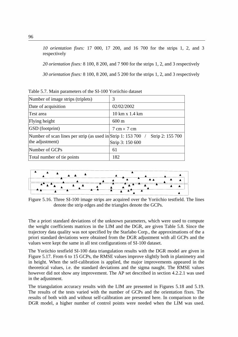
96

10 orientation fixes: 17 000, 17 200, and 16 700 for the strips 1, 2, and 3 respectively

20 orientation fixes: 8 100, 8 200, and 7 900 for the strips 1, 2, and 3 respectively

30 orientation fixes: 8 100, 8 200, and 5 200 for the strips 1, 2, and 3 respectively

Table 5.7. Main parameters of the SI-100 Yoriichio dataset

Number of image strips (triplets) 3

Date of acquisition 02/02/2002

Test area 10 km x 1.4 km

Flying height 600 m

GSD (footprint) 7 cm 7 cm

Number of scan lines per strip (as used in the adjustment)

Strip 1: 153 700 / Strip 2: 155 700 Strip 3: 150 600

Number of GCPs 61

Total number of tie points 182

Figure 5.16. Three SI-100 image strips are acquired over the Yoriichio testfield. The lines denote the strip edges and the triangles denote the GCPs.

The a priori standard deviations of the unknown parameters, which were used to compute the weight coefficients matrices in the LIM and the DGR, are given Table 5.8. Since the trajectory data quality was not specified by the Starlabo Corp., the approximations of the a priori standard deviations were obtained from the DGR adjustment with all GCPs and the values were kept the same in all test configurations of SI-100 dataset.

The Yoriichio testfield SI-100 data triangulation results with the DGR model are given in Figure 5.17. From 6 to 15 GCPs, the RMSE values improve slightly both in planimetry and in height. When the self-calibration is applied, the major improvements appeared in the theoretical values, i.e. the standard deviations and the sigma naught. The RMSE values however did not show any improvement. The AP set described in section 4.2.2.1 was used in the adjustment.

The triangulation accuracy results with the LIM are presented in Figures 5.18 and 5.19. The results of the tests varied with the number of GCPs and the orientation fixes. The results of both with and without self-calibration are presented here. In comparison to the DGR model, a higher number of control points were needed when the LIM was used.

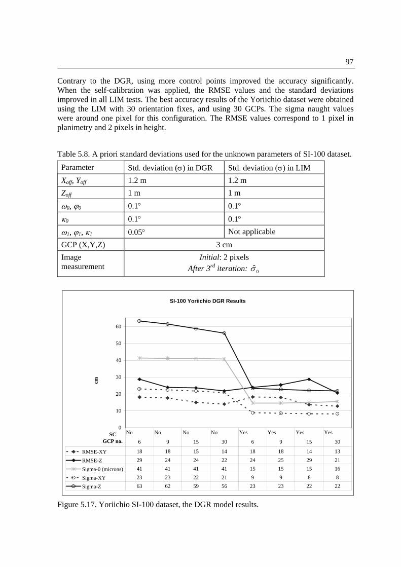
97

Contrary to the DGR, using more control points improved the accuracy significantly. When the self-calibration was applied, the RMSE values and the standard deviations improved in all LIM tests. The best accuracy results of the Yoriichio dataset were obtained using the LIM with 30 orientation fixes, and using 30 GCPs. The sigma naught values were around one pixel for this configuration. The RMSE values correspond to 1 pixel in planimetry and 2 pixels in height.

Table 5.8. A priori standard deviations used for the unknown parameters of SI-100 dataset.

Parameter Std. deviation () in DGR Std. deviation () in LIM

Xoff, Yoff 1.2 m 1.2 m

Zoff 1 m 1 m

0, 0 0.1 0.1

0 0.1 0.1

1, 1, 1 0.05 Not applicable

GCP (X,Y,Z) 3 cm

Image measurement

Initial: 2 pixels

After 3rd iteration: 0

SI-100 Yoriichio DGR Results

0

10

20

30

40

50

60

SC GCP no.

cm

RMSE-XY 18 18 15 14 18 18 14 13

RMSE-Z 29 24 24 22 24 25 29 21

Sigma-0 (microns) 41 41 41 41 15 15 15 16

Sigma-XY 23 23 22 21 9 9 8 8

Sigma-Z 63 62 59 56 23 23 22 22

No No No No Yes Yes Yes Yes

6 9 15 30 6 9 15 30

Figure 5.17. Yoriichio SI-100 dataset, the DGR model results.

98

Yoriichio LIM Results with 15 GCPs

0

20

40

60

80

100

Ori fix no. SC

cm

RMSE-XY 13 18 43 36 11 12 12 13

RMSE-Z 28 31 39 37 26 23 23 20

Sigma-0 (microns) 40 40 41 41 10 8 7 8

Sigma-XY 24 33 49 50 6 7 10 10

Sigma-Z 68 85 105 106 18 17 20 20

5 10 20 30 5 10 20 30

No No No No Yes Yes Yes Yes

Figure 5.18. Yoriichio SI-100 dataset LIM results with 15 GCPs.

Yoriichio LIM results with 30 GCPs

0

10

20

30

40

50

60

70

80

Ori. fix no. SC

cm

RMSE-XY 11 10 20 19 10 7 8 8

RMSE-Z 21 23 26 29 19 17 14 16

Sigma-0 (microns) 40 40 40 40 11 8 7 8

Sigma-XY 22 25 31 32 6 5 6 6

Sigma-Z 60 66 79 82 17 14 15 16

5 10 20 30 5 10 20 30

No No No No Yes Yes Yes Yes

Figure 5.19. Yoriichio SI-100 dataset LIM results with 30 GCPs.

99

5.1.2 Findings and Discussion

Considering the Yoriichio SI-290 dataset, using three different block configurations and the LIM, the accuracy results of the best cases are as following:

single strip: 1.1 pixels in planimetry and 2.1 pixels in height using 11 control points;

2-strips: 1.6 pixels in planimetry and 3.3 pixels in height using 12 control points;

4-strips: 1.1 pixels in planimetry and 2.4 pixels in height using 12 control points.

The sigma naught values of the LIM tests with 45 orientation fixes were around one pixel for all three block configurations. The increase in the number of the LIM orientation fixes has a positive effect on the estimated sigma naught values.

With the cross-strip configuration of 4-strips, it was possible to obtain a relatively stable system even with 3 control points. With the use of the LIM and a high number of tie points, thus higher number of orientation fixes, the sigma naught and the standard deviations of the ground coordinates became smaller. The positive effect of trajectory modeling with the LIM was more significant in height values. The DGR model was not adequate to model the systematic errors of the trajectory with the nine modeling parameters defined by the algorithm. Using the DGR model, the following accuracy results were achieved:

single strip: 2.5 pixels in planimetry and 4.9 pixels in height using 11 control points;

2-strips: 3.3 pixels in planimetry and 6.3 pixels in height using 12 control points;

4-strips: 3.3 pixels in planimetry and 7.8 pixels in height using 12 control points.

One of the main problems of the test data was very low GCP image quality due to poor signalization on the ground. For an adequate and comprehensive accuracy testing, well-signalized and well-distributed control points are crucial. The quality of the trajectory data has a major effect on the accuracy of the results. The trajectory data used in these tests most probably had a high noise level. Due to these errors, trajectory modeling with the LIM was very important for high adjustment accuracy.

An efficient block configuration and control point distribution was important to improve the system accuracy due to two reasons. First, the correlations between the exterior orientation parameters were very high and they should be controlled by the network geometry as well as the stochastical model of the adjustment. The 2-strips block had the disadvantage of inadequate distribution of control points. With a better control point distribution, the exterior orientation parameters could be estimated more precisely.

Secondly, with an efficient block configuration it was possible to reduce the number of control points to reach a certain accuracy level. In the LIM case, the sigma and RMSE values of the single strip tests performed with 6 GCPs were similar to the those of 4-strips tests performed with 3 GCPs. Single strip tests have shown that a single strip had poorer geometry and a high number of control points was necessary for the system stability and trajectory modeling. With a small number of control points (<=6), it was better to use the DGR model or the LIM with smaller number of orientation fixes.

100

Considering the SI-100 Yoriichio dataset, the DGR model required less control points in comparison to the LIM, but the accuracy remained the same with more control points. The self-calibration with the DGR model improved the sigma naught and the standard deviations only. The LIM modeled the trajectory errors better, although more control points were needed. In addition, the APs helped to improve the overall system accuracy in all LIM tests. A high number of orientation fixes provided only slightly better triangulation accuracy. However more control points were needed to keep the system stable in this case.

In both datasets, the blocks suffered from insufficient image quality, bad definition of signalized points, and problems in GPS/INS processing. Therefore, the results shown here should be examined with some care and should not be generalized.

101

5.2 The ADS40 Sensor

The ADS40 sensor is developed by Leica Geosystems, Heerbrugg, Switzerland. Simultaneous multiple image acquisitions are performed with the TLS principle. Therefore, the main design principles are similar to the STARIMAGER sensors of the former Starlabo Corporation, Tokyo. The basic design principles are given by Sandau et al. (2000). The ADS40 is accommodated in the PAV30 gyro-stabilized mount. The ADS40 sensor and its onboard installation are demonstrated in Figure 5.20.

The Linear Array CCD arrangements of different ADS40 sensors can be customized based on the user demands prior to production. Therefore, the sensors used in the following testfields have slight differences in terms of spectral characteristics and the positions of the CCD arrays in the focal plane and the viewing angles. The sensors’ main characteristics are given in the sections of respective datasets.

5.2.1 Applications to Testfields

Imagery of two different ADS40 sensors acquired over two different testfields, the Vaihingen/Enz testfield, Germany, and the Pavia testfield, Italy, were investigated in this study. The Vaihingen/Enz tests flights were part of the EuroSDR (European Spatial Data Research) project “Digital Camera Calibration”, together with the test flights of two aerial Frame Array sensors. As a project participant, we have also processed a part of the ADS40 dataset at the IGP, ETH Zurich. The test results were published in Kocaman et al. (2006). In addition to these results, the triangulation results of two other research groups are provided by Cramer (2007). All results were at the same level of accuracy when self-calibration was applied.

The Pavia test flights were performed in the year 2004 by the CGR Company, Italy, with an ADS40 sensor, which has a specially designed Linear Array CCD arrangement in the focal plane. The ADS40 datasets from two different flying heights were processed at the IGP, ETH Zurich, and the Geomatics Laboratory at the University of Pavia. The results were published before in Casella et al. (2007a, 2007b) and Kocaman et al. (2007).

The IGP results of both the Vaihingen/Enz and the Pavia ADS40 datasets are presented in more details in the following sections together with discussions and concluding remarks

5.2.1.1 Vaihingen/Enz, Germany

The Vaihingen/Enz test site was established by the Institute for Photogrammetry (IFP), University of Stuttgart, in 1995 originally for the geometrical performance test of the DPA sensor. The test site itself is located about 20km north-west of Stuttgart in a hilly area providing several types of vegetation and land use, a mostly rural area with smaller forests and villages. There exist more than 200 signalized and natural control points in the area (Cramer, 2005).

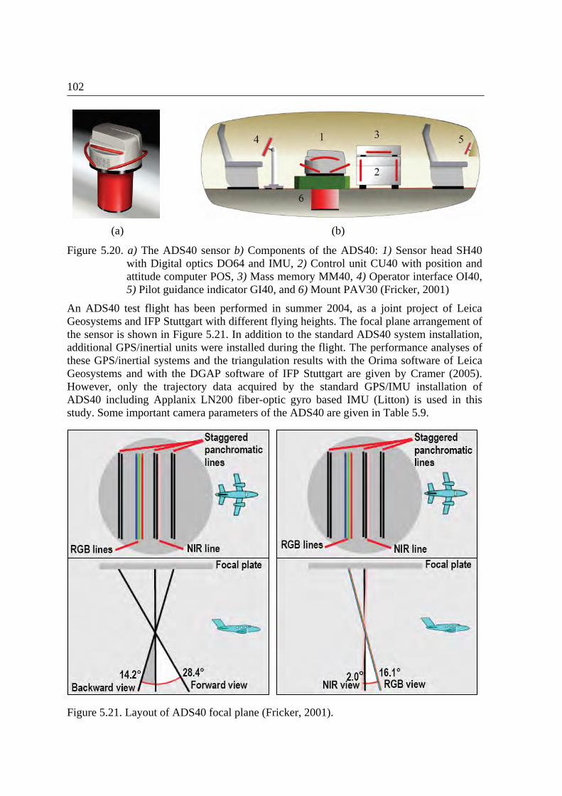
102

Figure 5.20. a) The ADS40 sensor b) Components of the ADS40: 1) Sensor head SH40 with Digital optics DO64 and IMU, 2) Control unit CU40 with position and attitude computer POS, 3) Mass memory MM40, 4) Operator interface OI40, 5) Pilot guidance indicator GI40, and 6) Mount PAV30 (Fricker, 2001)

An ADS40 test flight has been performed in summer 2004, as a joint project of Leica Geosystems and IFP Stuttgart with different flying heights. The focal plane arrangement of the sensor is shown in Figure 5.21. In addition to the standard ADS40 system installation, additional GPS/inertial units were installed during the flight. The performance analyses of these GPS/inertial systems and the triangulation results with the Orima software of Leica Geosystems and with the DGAP software of IFP Stuttgart are given by Cramer (2005). However, only the trajectory data acquired by the standard GPS/IMU installation of ADS40 including Applanix LN200 fiber-optic gyro based IMU (Litton) is used in this study. Some important camera parameters of the ADS40 are given in Table 5.9.

Figure 5.21. Layout of ADS40 focal plane (Fricker, 2001).

(a) (b)

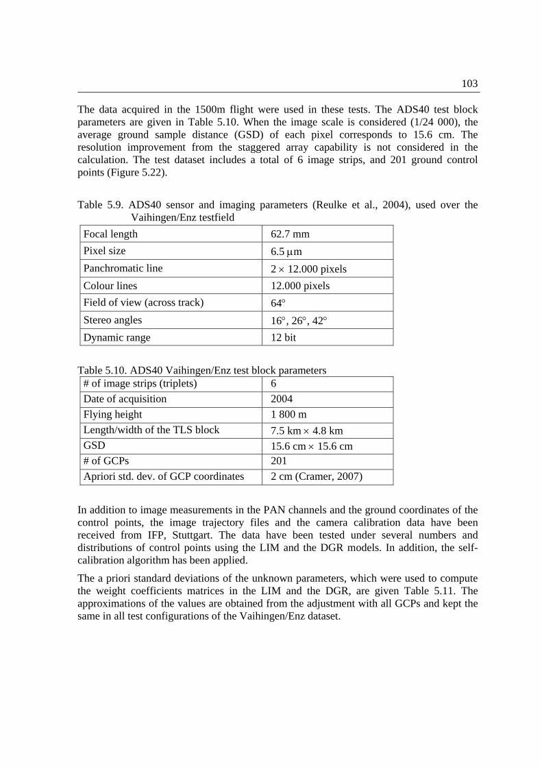
103

The data acquired in the 1500m flight were used in these tests. The ADS40 test block parameters are given in Table 5.10. When the image scale is considered (1/24 000), the average ground sample distance (GSD) of each pixel corresponds to 15.6 cm. The resolution improvement from the staggered array capability is not considered in the calculation. The test dataset includes a total of 6 image strips, and 201 ground control points (Figure 5.22).

Table 5.9. ADS40 sensor and imaging parameters (Reulke et al., 2004), used over the

Vaihingen/Enz testfield

Focal length 62.7 mm

Pixel size 6.5 m

Panchromatic line 2 12.000 pixels

Colour lines 12.000 pixels

Field of view (across track) 64 Stereo angles 16, 26, 42 Dynamic range 12 bit

Table 5.10. ADS40 Vaihingen/Enz test block parameters # of image strips (triplets) 6

Date of acquisition 2004

Flying height 1 800 m

Length/width of the TLS block 7.5 km 4.8 km GSD 15.6 cm 15.6 cm # of GCPs 201

Apriori std. dev. of GCP coordinates 2 cm (Cramer, 2007)

In addition to image measurements in the PAN channels and the ground coordinates of the control points, the image trajectory files and the camera calibration data have been received from IFP, Stuttgart. The data have been tested under several numbers and distributions of control points using the LIM and the DGR models. In addition, the self-calibration algorithm has been applied.

The a priori standard deviations of the unknown parameters, which were used to compute the weight coefficients matrices in the LIM and the DGR, are given Table 5.11. The approximations of the values are obtained from the adjustment with all GCPs and kept the same in all test configurations of the Vaihingen/Enz dataset.

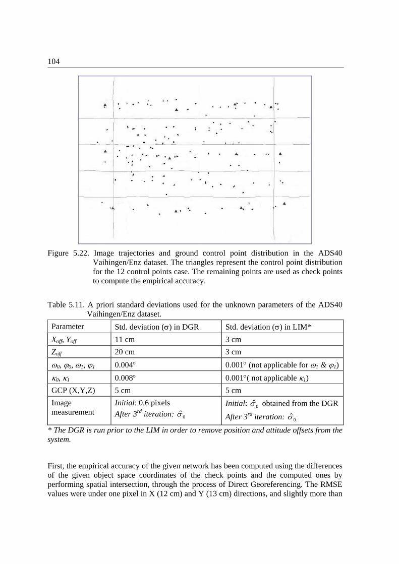
104

Figure 5.22. Image trajectories and ground control point distribution in the ADS40 Vaihingen/Enz dataset. The triangles represent the control point distribution for the 12 control points case. The remaining points are used as check points to compute the empirical accuracy.

Table 5.11. A priori standard deviations used for the unknown parameters of the ADS40

Vaihingen/Enz dataset.

Parameter Std. deviation () in DGR Std. deviation () in LIM*

Xoff, Yoff 11 cm 3 cm

Zoff 20 cm 3 cm

0, 0, 1, 1 0.004 0.001 (not applicable for 1 & 1)

0, 1 0.008 0.001( not applicable 1)

GCP (X,Y,Z) 5 cm 5 cm

Image measurement

Initial: 0.6 pixels

After 3rd iteration: 0 Initial: 0 obtained from the DGR

After 3rd iteration: 0

* The DGR is run prior to the LIM in order to remove position and attitude offsets from the system.

First, the empirical accuracy of the given network has been computed using the differences of the given object space coordinates of the check points and the computed ones by performing spatial intersection, through the process of Direct Georeferencing. The RMSE values were under one pixel in X (12 cm) and Y (13 cm) directions, and slightly more than

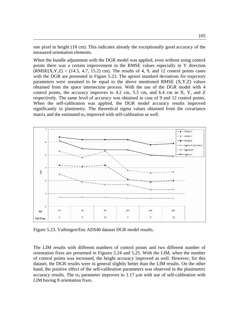
105

one pixel in height (18 cm). This indicates already the exceptionally good accuracy of the measured orientation elements.

When the bundle adjustment with the DGR model was applied, even without using control points there was a certain improvement in the RMSE values especially in Y direction (RMSE(X,Y,Z) = (14.5, 4.7, 15.2) cm). The results of 4, 9, and 12 control points cases with the DGR are presented in Figure 5.23. The apriori standard deviations for trajectory parameters were assumed to be equal to the above mentioned RMSE (X,Y,Z) values obtained from the space intersection process. With the use of the DGR model with 4 control points, the accuracy improves to 4.2 cm, 5.3 cm, and 6.4 cm in X, Y, and Z respectively. The same level of accuracy was obtained in case of 9 and 12 control points. When the self-calibration was applied, the DGR model accuracy results improved significantly in planimetry. The theoretical sigma values obtained from the covariance matrix and the estimated 0 improved with self-calibration as well.

Figure 5.23. Vaihingen/Enz ADS40 dataset DGR model results.

The LIM results with different numbers of control points and two different number of orientation fixes are presented in Figures 5.24 and 5.25. With the LIM, when the number of control points was increased, the height accuracy improved as well. However, for this dataset, the DGR results were in general slightly better than the LIM results. On the other hand, the positive effect of the self-calibration parameters was observed in the planimetric accuracy results. The 0 parameter improves to 1.17 m with use of self-calibration with LIM having 8 orientation fixes.

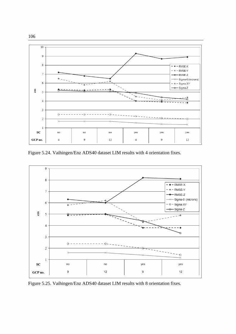
106

Figure 5.24. Vaihingen/Enz ADS40 dataset LIM results with 4 orientation fixes.

Figure 5.25. Vaihingen/Enz ADS40 dataset LIM results with 8 orientation fixes.

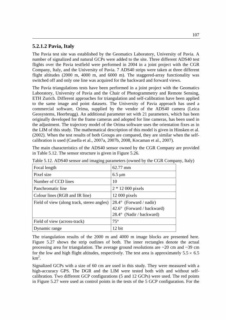
107

5.2.1.2 Pavia, Italy

The Pavia test site was established by the Geomatics Laboratory, University of Pavia. A number of signalized and natural GCPs were added to the site. Three different ADS40 test flights over the Pavia testfield were performed in 2004 in a joint project with the CGR Company, Italy, and the University of Pavia. 7 ADS40 strips were taken at three different flight altitudes (2000 m, 4000 m, and 6000 m). The staggered-array functionality was switched off and only one line was acquired for the backward and forward views.

The Pavia triangulations tests have been performed in a joint project with the Geomatics Laboratory, University of Pavia and the Chair of Photogrammetry and Remote Sensing, ETH Zurich. Different approaches for triangulation and self-calibration have been applied to the same image and point datasets. The University of Pavia approach has used a commercial software, Orima, supplied by the vendor of the ADS40 camera (Leica Geosystems, Heerbrugg). An additional parameter set with 21 parameters, which has been originally developed for the frame cameras and adopted for line cameras, has been used in the adjustment. The trajectory model of the Orima software uses the orientation fixes as in the LIM of this study. The mathematical description of this model is given in Hinsken et al. (2002). When the test results of both Groups are compared, they are similar when the self-calibration is used (Casella et al., 2007a, 2007b, 2008, Kocaman et al., 2007).

The main characteristics of the ADS40 sensor owned by the CGR Company are provided in Table 5.12. The sensor structure is given in Figure 5.26.

Table 5.12. ADS40 sensor and imaging parameters (owned by the CGR Company, Italy)

Focal length 62.77 mm

Pixel size 6.5 μm

Number of CCD lines 10

Panchromatic line 2 * 12 000 pixels

Colour lines (RGB and IR line) 12 000 pixels

Field of view (along track, stereo angles)

28.4° (Forward / nadir) 42.6° (Forward / backward) 28.4° (Nadir / backward)

Field of view (across-track) 75°

Dynamic range 12 bit

The triangulation results of the 2000 m and 4000 m image blocks are presented here. Figure 5.27 shows the strip outlines of both. The inner rectangles denote the actual processing area for triangulation. The average ground resolutions are ~20 cm and ~39 cm for the low and high flight altitudes, respectively. The test area is approximately 5.5 6.5 km2.

Signalized GCPs with a size of 60 cm are used in this study. They were measured with a high-accuracy GPS. The DGR and the LIM were tested both with and without self-calibration. Two different GCP configurations (5 and 12 GCPs) were used. The red points in Figure 5.27 were used as control points in the tests of the 5 GCP configuration. For the

108

12 GCP configuration, the green points and the four red points in the corners were used. The black points were used as independent check points in all tests.

Figure 5.26. Structure of the ADS40 owned by CGR and used to acquire the studied imagery (Casella & Franzini, 2006).

Figure 5.27. Structures of the 2000 m (red) and 4000 m (blue) blocks and the distributions of GCPs (Kocaman et al., 2007).

The image coordinate measurements of the control points were manually performed at the University of Pavia and provided to the our Group. 46 and 50 signalized control points were measured on the images of 2000 m flight and 4000 m flight, respectively. The visibility of the points in the images of all flight datasets are shown in Figure 5.28. Tie points were extracted and measured automatically with the APM of Socet Set.

(a) (b)

(c) Figure 5.28. Visibility of a GCP in (a) the 2000m block (b) the 4000m block (c) the

6000m block (Casella et al., 2007b).

1 pixel

12.000 pixels

2 Red 2 Green

1 Blue 1 NIR

2 2 Panchromatic

109

The a priori standard deviations of the unknown parameters, which are used to compute the weight coefficients matrices in the LIM and the DGR, are given Table 5.13. The approximations of the values are obtained from the adjustment with all GCPs and kept the same in all test configurations of the Pavia dataset.

Table 5.13. A priori standard deviations used for the unknown parameters of the ADS40

Pavia dataset.

Parameter Std. deviation () in the DGR and the LIM

Xoff, Yoff 10 cm

Zoff 20 cm

0, 0, 1, 1 0.0054

0, 1 0.0081

GCP (X,Y,Z) XY: 1.5 cm, Z: 2 cm

Image measurement Initial: 1/3 pixel (=2.2 microns)

Direct georeferencing results: Direct georeferencing was performed using multiple weighted forward intersection. The results are given in Table 5.14. Both datasets show systematic error behaviour, as can be seen from the mean of the residuals, especially in height.

Table 5.14. The ADS40 Pavia datasets, the results of direct georeferencing

Flight/parameter 2000 m block 4000 m block

Component X (m) Y (m) Z (m) X (m) Y (m) Z (m)

RMSE 0.12 0.10 0.65 0.32 0.57 1.79

Mean 0.01 -0.01 -0.57 -0.14 0.34 -1.78

Sigma 0.10 0.10 0.22 0.15 0.18 0.39

The sigma variable in Table 5.14 is computed via error propogation from the covariance matrix of spatial intersection according to:

X

XX n

i2ˆ

ˆ

Y

YY n

i2ˆ

ˆ

Z

ZZ n

i2ˆ

ˆ

with nX nY, nZ number of point coordinates used for the computation.

Further investigations from Casella and Franzini (2008) have shown that the main factor of the systematic errors came from the camera calibration provided by the vendor. The APs are found mostly significant in the adjustment tests presented below.

(5.1)

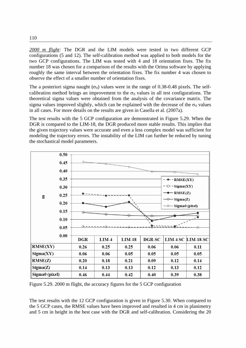
110

2000 m flight: The DGR and the LIM models were tested in two different GCP configurations (5 and 12). The self-calibration method was applied to both models for the two GCP configurations. The LIM was tested with 4 and 18 orientation fixes. The fix number 18 was chosen for a comparison of the results with the Orima software by applying roughly the same interval between the orientation fixes. The fix number 4 was chosen to observe the effect of a smaller number of orientation fixes.

The a posteriori sigma naught (0) values were in the range of 0.38-0.48 pixels. The self-calibration method brings an improvement to the 0 values in all test configurations. The theoretical sigma values were obtained from the analysis of the covariance matrix. The sigma values improved slightly, which can be explained with the decrease of the 0 values in all cases. For more details on the results are given in Casella et al. (2007a).

The test results with the 5 GCP configuration are demonstrated in Figure 5.29. When the DGR is compared to the LIM-18, the DGR produced more stable results. This implies that the given trajectory values were accurate and even a less complex model was sufficient for modeling the trajectory errors. The instability of the LIM can further be reduced by tuning the stochastical model parameters.

Figure 5.29. 2000 m flight, the accuracy figures for the 5 GCP configuration

The test results with the 12 GCP configuration is given in Figure 5.30. When compared to the 5 GCP cases, the RMSE values have been improved and resulted in 4 cm in planimetry and 5 cm in height in the best case with the DGR and self-calibration. Considering the 20

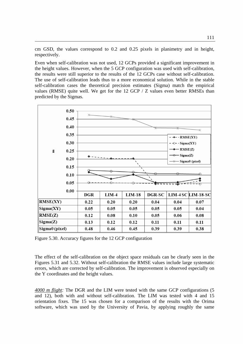
111

cm GSD, the values correspond to 0.2 and 0.25 pixels in planimetry and in height, respectively.

Even when self-calibration was not used, 12 GCPs provided a significant improvement in the height values. However, when the 5 GCP configuration was used with self-calibration, the results were still superior to the results of the 12 GCPs case without self-calibration. The use of self-calibration leads thus to a more economical solution. While in the stable self-calibration cases the theoretical precision estimates (Sigma) match the empirical values (RMSE) quite well. We get for the 12 GCP / Z values even better RMSEs than predicted by the Sigmas.

Figure 5.30. Accuracy figures for the 12 GCP configuration

The effect of the self-calibration on the object space residuals can be clearly seen in the Figures 5.31 and 5.32. Without self-calibration the RMSE values include large systematic errors, which are corrected by self-calibration. The improvement is observed especially on the Y coordinates and the height values.

4000 m flight: The DGR and the LIM were tested with the same GCP configurations (5 and 12), both with and without self-calibration. The LIM was tested with 4 and 15 orientation fixes. The 15 was chosen for a comparison of the results with the Orima software, which was used by the University of Pavia, by applying roughly the same

112

interval between the orientation fixes. The 4 was chosen as orientation fix number to observe the effect of a smaller number of orientation fixes. The a posteriori 0 values of all tests were in the range of 0.44-0.52 pixels. A graphical representation of the results of the 5 and 12 GCP cases are provided in Figures 5.33 and 5.34. The test results without self-calibration show large systematic errors, which were corrected by self-calibration (Figures 5.35 and 5.36).

The RMSE values obtained from the tests without self-calibration were between 0.8-1.0 pixels for planimetry, and 1.9-2.4 pixels for height. The LIM performed better than the DGR in height. Also, the use of 12 GCPs improved the RMSE height values slightly. The self-calibration improved the RMSE results. They were in the range of 0.18-0.24 pixels for planimetry and 0.31-0.38 pixels for height. The DGR and the LIM results with self-calibration were very similar in planimetry, while in height the DGR was slightly better. The results of the 5 and 12 GCP cases were very similar in all self-calibration tests.

-1000 0 1000 2000 3000 4000 5000-3500

-3000

-2500

-2000

-1500

-1000

-500

0

500

1000

1500

2000

X [m]

Y [

m]

1 2

8

18

23

28 29

3637

39

45

49

3

56

7

910 11

12 13

1415

16 17

20

22

24 2526

27

30 31 32

3334

35

3840

41 4243

44

46 47

48

10 cm

Figure 5.31. Object space residuals for the DGR model with 12 GCPs without self-calibration

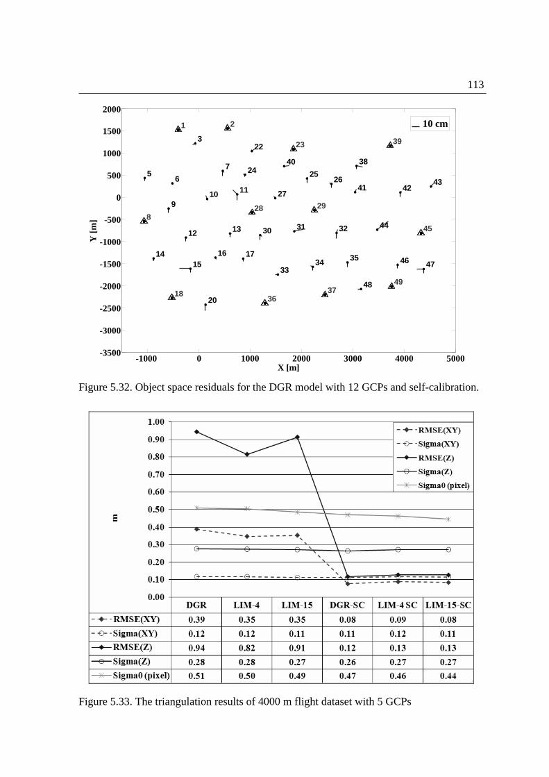
113

-1000 0 1000 2000 3000 4000 5000-3500

-3000

-2500

-2000

-1500

-1000

-500

0

500

1000

1500

2000

X [m]

Y [

m]

1 2

8

18

23

28 29

3637

39

45

49

3

56

7

910 11

12 13

1415

16 17

20

22

24 2526

27

30 31 32

3334

35

3840

41 4243

44

46 47

48

10 cm

Figure 5.32. Object space residuals for the DGR model with 12 GCPs and self-calibration.

Figure 5.33. The triangulation results of 4000 m flight dataset with 5 GCPs

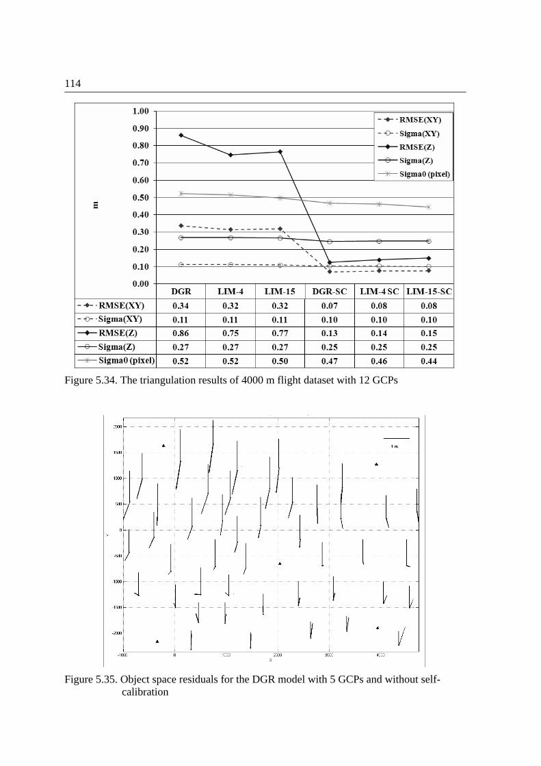
114

Figure 5.34. The triangulation results of 4000 m flight dataset with 12 GCPs

Figure 5.35. Object space residuals for the DGR model with 5 GCPs and without self-calibration

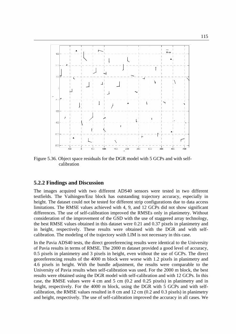
115

Figure 5.36. Object space residuals for the DGR model with 5 GCPs and with self-calibration

5.2.2 Findings and Discussion

The images acquired with two different ADS40 sensors were tested in two different testfields. The Vaihingen/Enz block has outstanding trajectory accuracy, especially in height. The dataset could not be tested for different strip configurations due to data access limitations. The RMSE values achieved with 4, 9, and 12 GCPs did not show significant differences. The use of self-calibration improved the RMSEs only in planimetry. Without consideration of the improvement of the GSD with the use of staggered array technology, the best RMSE values obtained in this dataset were 0.21 and 0.37 pixels in planimetry and in height, respectively. These results were obtained with the DGR and with self-calibration. The modeling of the trajectory wsith LIM is not necessary in this case.

In the Pavia ADS40 tests, the direct georeferencing results were identical to the University of Pavia results in terms of RMSE. The 2000 m dataset provided a good level of accuracy, 0.5 pixels in planimetry and 3 pixels in height, even without the use of GCPs. The direct georeferencing results of the 4000 m block were worse with 1.2 pixels in planimetry and 4.6 pixels in height. With the bundle adjustment, the results were comparable to the University of Pavia results when self-calibration was used. For the 2000 m block, the best results were obtained using the DGR model with self-calibration and with 12 GCPs. In this case, the RMSE values were 4 cm and 5 cm (0.2 and 0.25 pixels) in planimetry and in height, respectively. For the 4000 m block, using the DGR with 5 GCPs and with self-calibration, the RMSE values resulted in 8 cm and 12 cm (0.2 and 0.3 pixels) in planimetry and height, respectively. The use of self-calibration improved the accuracy in all cases. We

116

should also note that the staggered array technology was switched off in the Pavia test flights.

Overall, the ADS40 tests showed that

- The APs were in general determinable under the given estimation model parameters. There were usually high correlations between the EO and APs in the initial set, which were treated by the parameter removal algorithm in an iterative approach. When the RMSE values are analyzed at each iteration, differences between the full and reduced sets of APs were found very small and negligible, showing the fact that there was no significant disturbance on the object point coordinates which was caused by the APs. This fact was also proved by the trace check algorithm.

- An accurate image and trajectory dataset can reach the geometric accuracy potential even with few well-defined and signalized GCPs.

117

5.3 The ALOS/PRISM Sensor

5.3.1 Introduction

The Chair of Photogrammetry and Remote Sensing, ETH Zurich, is a member of the JAXA (Japan Aerospace Exploration Agency) Cal/Val team for the ALOS/PRISM sensor. Since the launch of the satellite, the calibration and validation work has been performed. Software and algorithms have been developed and tested using data from several testfields for this purpose.

Two of the trajectory models, the PPM and the DGR model, are used for georeferencing and calibration with a specially developed set of APs, which are described in Chapter 4.2.2.2. The LIM is not applied here, since the PPM provides sufficient level of complexity to model errors of the satellite trajectory. In addition, a small number of segments are applicable with this model whereas a minimum of 4 orientation fixes are required with the LIM. The AP set and the trajectory models are described in Chapter 4.

A brief overview of the PRISM sensor and data characteristics, pre-processing methods, the results of the sensor orientation and calibration obtained in a number of testfields, and an analysis of the results are given in the following sections. Details of different phases of sensor calibration are given in chronological order. The algorithms have been updated during the calibration work. Therefore, there are differences in the applications.

Georeferencing results from a number of other high-resolution satellite (HRS) images are presented in the next section for a comparison with the findings from PRISM images.

5.3.1.1 PRISM Sensor Description

The new generation Japanese remote sensing satellite ALOS (Advanced Land Observing Satellite) has three remote-sensing instruments onboard: PRISM (Panchromatic Remote-sensing Instrument for Stereo Mapping), AVNIR-2 (Advanced Visible and Near Infrared Radiometer type-2), and PALSAR (Cloud Phased Array type L-band Synthetic Aperture Radar). A StarTracker and a GPS antenna are installed on the satellite in order to measure the platform rotation and position, respectively. A graphical demonstration of the satellite is provided in Figure 5.37.

PRISM is a panchromatic radiometer with 2.5-meter spatial resolution. It has three optical systems for forward, nadir and backward view working with pushbroom principle (see Figures 2.2 and 2.5 in Chapter 2). There are two different image acquisition modes according to chosen swath width. In triplet imaging mode, the swath width is 35 km. If 70 km swath width is preferred, only the nadir and backward cameras work simultaneously. The main characteristics of the PRISM sensor are given in Table 5.15.

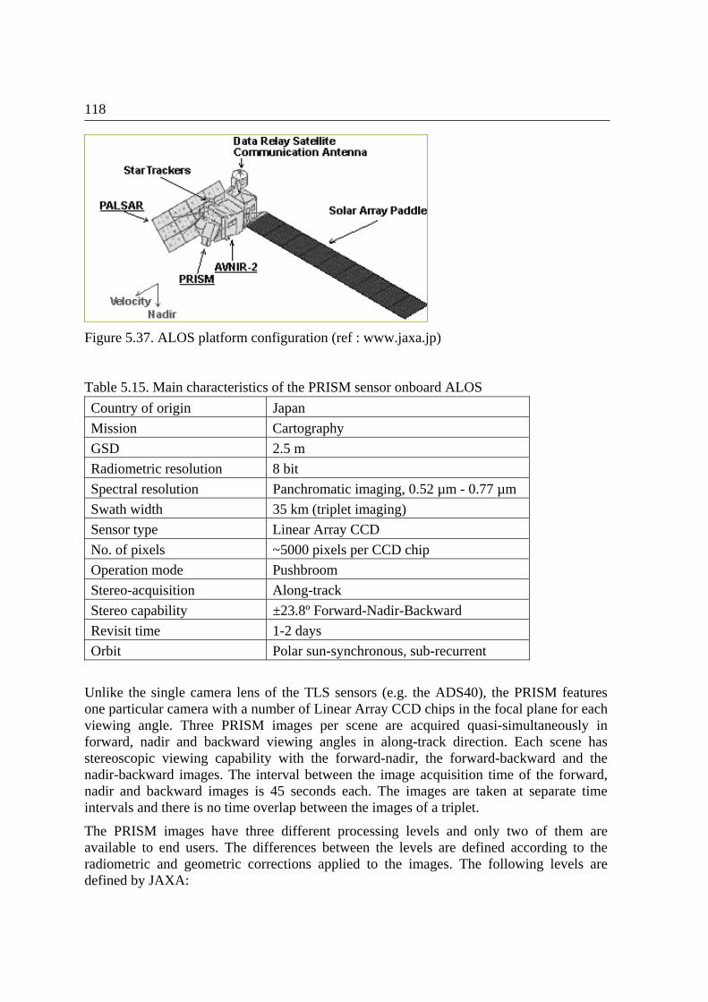
118

Figure 5.37. ALOS platform configuration (ref : www.jaxa.jp)

Table 5.15. Main characteristics of the PRISM sensor onboard ALOS

Country of origin Japan

Mission Cartography

GSD 2.5 m

Radiometric resolution 8 bit

Spectral resolution Panchromatic imaging, 0.52 µm - 0.77 µm

Swath width 35 km (triplet imaging)

Sensor type Linear Array CCD

No. of pixels ~5000 pixels per CCD chip

Operation mode Pushbroom

Stereo-acquisition Along-track

Stereo capability ±23.8º Forward-Nadir-Backward

Revisit time 1-2 days

Orbit Polar sun-synchronous, sub-recurrent

Unlike the single camera lens of the TLS sensors (e.g. the ADS40), the PRISM features one particular camera with a number of Linear Array CCD chips in the focal plane for each viewing angle. Three PRISM images per scene are acquired quasi-simultaneously in forward, nadir and backward viewing angles in along-track direction. Each scene has stereoscopic viewing capability with the forward-nadir, the forward-backward and the nadir-backward images. The interval between the image acquisition time of the forward, nadir and backward images is 45 seconds each. The images are taken at separate time intervals and there is no time overlap between the images of a triplet.

The PRISM images have three different processing levels and only two of them are available to end users. The differences between the levels are defined according to the radiometric and geometric corrections applied to the images. The following levels are defined by JAXA:

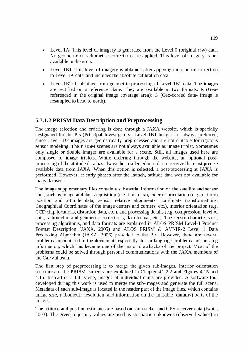
119

Level 1A: This level of imagery is generated from the Level 0 (original raw) data. No geometric or radiometric corrections are applied. This level of imagery is not available to the users.

Level 1B1: This level of imagery is obtained after applying radiometric correction to Level 1A data, and includes the absolute calibration data.

Level 1B2: It obtained from geometric processing of Level 1B1 data. The images are rectified on a reference plane. They are available in two formats: R (Geo-referenced in the original image coverage area); G (Geo-corded data- image is resampled to head to north).

5.3.1.2 PRISM Data Description and Preprocessing

The image selection and ordering is done through a JAXA website, which is specially designated for the PIs (Principal Investigators). Level 1B1 images are always preferred, since Level 1B2 images are geometrically preprocessed and are not suitable for rigorous sensor modeling. The PRISM scenes are not always available as image triplet. Sometimes only single or double images are available for a scene. Still, all images used here are composed of image triplets. While ordering through the website, an optional post-processing of the attitude data has always been selected in order to receive the most precise available data from JAXA. When this option is selected, a post-processing at JAXA is performed. However, at early phases after the launch, attitude data was not available for many datasets.

The image supplementary files contain a substantial information on the satellite and sensor data, such as image and data acquisition (e.g. time data), exterior orientation (e.g. platform position and attitude data, sensor relative alignments, coordinate transformations, Geographical Coordinates of the image centers and corners, etc.), interior orientation (e.g. CCD chip locations, distortion data, etc.), and processing details (e.g. compression, level of data, radiometric and geometric corrections, data format, etc.). The sensor characteristics, processing algorithms, and data formats are explained in ALOS PRISM Level-1 Product Format Description (JAXA, 2005) and ALOS PRISM & AVNIR-2 Level 1 Data Processing Algorithm (JAXA, 2006) provided to the PIs. However, there are several problems encountered in the documents especially due to language problems and missing information, which has became one of the major drawbacks of the project. Most of the problems could be solved through personal communications with the JAXA members of the Cal/Val team.

The first step of preprocessing is to merge the given sub-images. Interior orientation structures of the PRISM cameras are explained in Chapter 4.2.2.2 and Figures 4.15 and 4.16. Instead of a full scene, images of individual chips are provided. A software tool developed during this work is used to merge the sub-images and generate the full scene. Metadata of each sub-image is located in the header part of the image files, which contains image size, radiometric resolution, and information on the unusable (dummy) parts of the images.

The attitude and position estimates are based on star tracker and GPS receiver data (Iwata, 2003). The given trajectory values are used as stochastic unknowns (observed values) in

120

the adjustment. The position data is given in the image supplementary files in two different coordinate systems (ECI- Earth Centered Inertial and ECR- Earth Centered Rotating systems). The ECR data are used directly in the computations. The position data is provided for 25 hours in one minute interval. Given the image acquisition time, the position data of each image line is interpolated using a 2nd order polynomial function. The accuracy of the position data is also provided in this file and usually equal to 1 m.

The attitude data was not available for some of the early PRISM images. Therefore, they were estimated in the adjustment. In later datasets, the attitude data was given in the image supplementary file. However, it was still not employed in some of the following datasets due to lack of proper data format description at the time of processing.

The provided attitude data is in quaternion format, which is composed of four elements to reconstruct the rotation matrix. The rotation matrix defines the transformation between the ECI (J2000) system to satellite coordinate system. First of all, a transformation between the ECI system to ECR system is required. The attitude data is given with 0.1 second interval for one orbit cycle (approximately 99 minutes). The following rotations are applied in a stepwise procedure for the ECI-to-ECR transformation for each attitude dataset.

To convert the J2000 values into TOD (True of Date) system, astronomic nutation and precession matrices are applied. Both matrices contain time dependent parameters.

Between the TOD and the ECR, the Greenwich Sidereal Time and polar motion matrices are applied to the data.

After the transformation into the ECR system, an interpolation is performed using a 2nd order polynomial function, in order to obtain the attitude data of each image line according to image acquisition time.

Since the trajectory data is defined in satellite coordinate system, after this step, it is transformed into the camera coordinate systems, which has its origin at the camera perspective center. In addition, before the triangulation, another transformation is applied to the trajectory data and the GCP coordinates to convert them into a local Cartesian coordinate system. The origin of the local coordinate system is taken as the center of the nadir image.

As a part of preprocessing, the given CCD chip positions have been interpolated for each pixel and transformed into the focal plane. The positions of the centers of three CCD pixel detectors (start, center, and end) for each CCD chip were provided by JAXA as a part of Cal/Val team work. First, a scale transformation was performed since the given values were defined on a virtual plane, which is parallel to the focal plane. Afterwards, a linear interpolation function was used to generate a look-up table for each camera, which contains the positions of all CCD pixels in image coordinate system. This step was necessary to adapt data into the software input format.

In addition to the CCD chip positions, the focal length of each PRISM camera and the CCD pixel size were provided by JAXA.

121

5.3.2 Applications to Testfields

Until now, 12 different PRISM image datasets have been processed in terms of triangulation and self-calibration and the results of most of them have been published in different scientific platforms (e.g. Gruen et al., 2007, Kocaman and Gruen 2007a, 2007b, 2008, etc.). In addition, DSMs (digital surface models) have been generated automatically for most of these testfields and some others from the PRISM images using the IGP software SAT-PP. The DSMs results are evaluated in Gruen et al. (2007), Gruen and Wolff (2007), Wolff and Gruen (2007).

Here the results of five testfields, Saitama and Okazaki, Japan, Piemont, Italy, Bern/Thun and Zurich/Winterthur, Switzerland, are presented. The Saitama dataset was the first one to be processed. The initial phases of calibration, software development, and testing have been performed with this dataset. The details are given in the following section.

The Zurich/Winterthur dataset represents the most recent status of the algorithm and software development, image quality, and the sensor calibration of JAXA. The results were therefore different from the other four earlier datasets, especially for the minimum GCP requirement to achieve sub-pixel accuracy.

5.3.2.1 Saitama, Japan

The Saitama testfield is located in the north-east of Tokyo, Japan. It was the first ALOS/PRISM Cal/Val dataset generated by JAXA. The PRISM images have been acquired in April, 2006. The main parameters of the dataset are given in Table 5.16. There are 203 ground control points measured on the images (Figure 5.38). The image measurements of the GCPs have been performed by JAXA, Japan. Many of the GCPs are closely located on the ground (Figure 5.39). 111 tie points were measured manually at the IGP in order to have denser image point distribution.

Table 5.16. Main parameters of the PRISM dataset acquired over the Saitama testfield.

Imaging Date 30.04.2006

Number of PRISM images 1 scene with forward, nadir and backward images

Viewing angles -23.8, 0, 23.8No. of GCPs 203

No. of tie points 111

The software development, additional parameter (AP) definition for self-calibration, and the testing have been initially performed with the Saitama dataset in a stepwise procedure. The image metadata extraction and generation of full image scene have been performed as the very first step. The supplementary data extraction part has evolved during testing, and further implementations are still necessary.

In the second step, the DGR model has been implemented for the multiple camera structure of the PRISM. No APs were defined at this step. Since no attitude data were available, they have been estimated using all GCPs. These values were used as rough approximations and the dataset was tested with 12 GCPs. The achieved theoretical and empirical accuracy

122

values were 1½ pixels. It should also be noted that the a priori standard deviations of the trajectory unknowns were 100 m for the position, 2 for the 0, 0, 0, and 0.2 for the 1,1, 1 parameters for a whole image (0.034/second), and did not represent the reality, especially due to the metadata interpretation problem. In addition, the interior orientation data were not precise, only the nominal values of focal length and the CCD pixel size were known, and CCD detector position information was missing.

In the next step, the scale and CCD line bending parameters (two parameters per image) have been added to the DGR model. Using the APs and correct weighting scheme (given in Table 5.17), the achieved RMSE values were (0.8 pixel) in planimetry and 2.8 m (1.1 pixel) in height. The a posteriori sigma naught was equal to 0.6 pixel. There were still strong systematic effects in the object space (Figure 5.40). In order to identify the sources of these errors, the residuals have been back projected into the image space. The back-projected error vectors indicated displacements in the relative positions of the CCD chips, in all three images. The image space residuals obtained from the Saitama tests are presented in Figures 5.41a,b,c. CCD center displacement parameters have been added to the model (Eq. 4.44a and 4.44b in Chapter 4) and the shifts could be compensated by these parameters.

Figure 5.38. GCP distribution in Saitama PRISM nadir image.

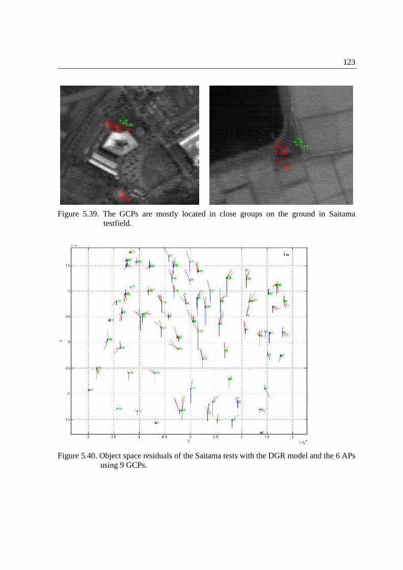
123

Figure 5.39. The GCPs are mostly located in close groups on the ground in Saitama testfield.

Figure 5.40. Object space residuals of the Saitama tests with the DGR model and the 6 APs using 9 GCPs.

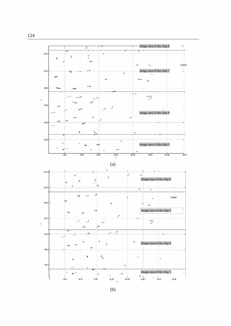
124

(a)

(b)

Image area of the chip 8

Image area of the chip 7

Image area of the chip 6

Image area of the chip 5

Image area of the chip 6

Image area of the chip 5

Image area of the chip 4

Image area of the chip 3

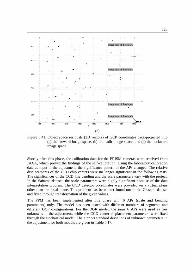
125

(c)

Figure 5.41. Object space residuals (3D vectors) of GCP coordinates back-projected into (a) the forward image space, (b) the nadir image space, and (c) the backward image space.

Shortly after this phase, the calibration data for the PRISM cameras were received from JAXA, which proved the findings of the self-calibration. Using the laboratory calibration data as input in the adjustment, the significance pattern of the APs changed. The relative displacements of the CCD chip centers were no longer significant in the following tests. The significances of the CCD line bending and the scale parameters vary with the project. In the Saitama dataset, the scale parameters were highly significant because of the data interpretation problem. The CCD detector coordinates were provided on a virtual plane other than the focal plane. This problem has been later found out in the Okazaki dataset and fixed through transformation of the given values.

The PPM has been implemented after this phase with 6 APs (scale and bending parameters) only. The model has been tested with different numbers of segments and different GCP configurations. For the DGR model, the same 6 APs were used as free unknowns in the adjustment, while the CCD center displacement parameters were fixed through the stochastical model. The a priori standard deviations of unknown parameters in the adjustment for both models are given in Table 5.17.

Image area of the chip 6

Image area of the chip 5

Image area of the chip 4

Image area of the chip 3

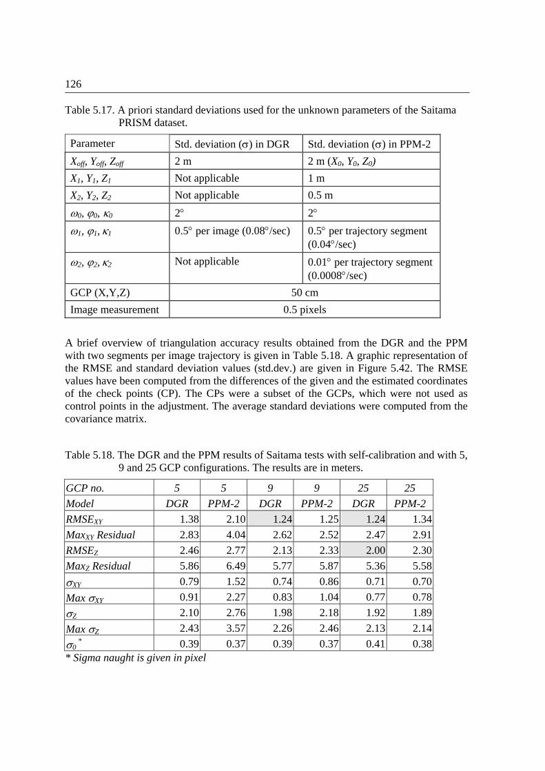
126

Table 5.17. A priori standard deviations used for the unknown parameters of the Saitama PRISM dataset.

Parameter Std. deviation () in DGR Std. deviation () in PPM-2

Xoff, Yoff, Zoff 2 m 2 m (X0, Y0, Z0)

X1, Y1, Z1 Not applicable 1 m

X2, Y2, Z2 Not applicable 0.5 m

0, 0, 0 2 2

1, 1, 1 0.5 per image (0.08/sec) 0.5 per trajectory segment (0.04/sec)

2, 2, 2 Not applicable 0.01 per trajectory segment (0.0008/sec)

GCP (X,Y,Z) 50 cm

Image measurement 0.5 pixels

A brief overview of triangulation accuracy results obtained from the DGR and the PPM with two segments per image trajectory is given in Table 5.18. A graphic representation of the RMSE and standard deviation values (std.dev.) are given in Figure 5.42. The RMSE values have been computed from the differences of the given and the estimated coordinates of the check points (CP). The CPs were a subset of the GCPs, which were not used as control points in the adjustment. The average standard deviations were computed from the covariance matrix.

Table 5.18. The DGR and the PPM results of Saitama tests with self-calibration and with 5, 9 and 25 GCP configurations. The results are in meters.

GCP no. 5 5 9 9 25 25

Model DGR PPM-2 DGR PPM-2 DGR PPM-2

RMSEXY 1.38 2.10 1.24 1.25 1.24 1.34

MaxXY Residual 2.83 4.04 2.62 2.52 2.47 2.91

RMSEZ 2.46 2.77 2.13 2.33 2.00 2.30

MaxZ Residual 5.86 6.49 5.77 5.87 5.36 5.58

XY 0.79 1.52 0.74 0.86 0.71 0.70

Max XY 0.91 2.27 0.83 1.04 0.77 0.78

Z 2.10 2.76 1.98 2.18 1.92 1.89

Max Z 2.43 3.57 2.26 2.46 2.13 2.14

0 *

0.39 0.37 0.39 0.37 0.41 0.38 * Sigma naught is given in pixel

127

Figure 5.42. Saitama tests accuracy results (RMSEs and standard deviations, computed for check point coordinates)

With the DGR, the RMSE values in planimetry were at sub-pixel level, even with only 5 GCPs. There was not much to gain by going from 5 over 9 to 25 GCPs. The RMSE values in height were similar in all versions (Figure 5.42). When the DGR and the PPM models are compared, the accuracy values were about at the same level in the 9 and 25 GCPs versions. However, the PPM requires a higher number of control points to be stable. The instability of the PPM has been indicated by the theoretical values (std. dev.) of the 5 GCPs case, which show significant differences between both models, although the sigma naught is almost equal. In all cases the standard deviations were clearly better than the related RMSEs. This shows the existence of small systematic residual errors.

5.3.2.2 Bern/Thun, Switzerland

The Bern/Thun testfield is located between the Bern and Thun cities of Switzerland. The testfield was set up by the Chair of Photogrammetry and Remote Sensing, ETH Zurich, under a contract with JAXA (Gruen et al., 2006). The coordinates of the GCPs were determined by GPS. The main parameters of the PRISM Bern/Thun dataset are given in Table 5.19. The testfield setup is demonstrated in Figure 5.43. All points were measured manually in the images. Similar to the Saitama dataset, the images suffer from a number of radiometric problems, leading to image artifacts, partially to fixed pattern noise. The reasons for those deficiencies are problems with black reference calibration (resulting in striping), jpeg-compression (resulting in blocking), saturation effects (mainly related to

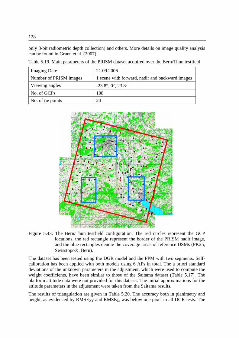
128

only 8-bit radiometric depth collection) and others. More details on image quality analysis can be found in Gruen et al. (2007).

Table 5.19. Main parameters of the PRISM dataset acquired over the Bern/Thun testfield

Imaging Date 21.09.2006

Number of PRISM images 1 scene with forward, nadir and backward images

Viewing angles -23.8, 0, 23.8 No. of GCPs 108

No. of tie points 24

Figure 5.43. The Bern/Thun testfield configuration. The red circles represent the GCP locations, the red rectangle represent the border of the PRISM nadir image, and the blue rectangles denote the coverage areas of reference DSMs (PK25, Swisstopo, Bern).

The dataset has been tested using the DGR model and the PPM with two segments. Self-calibration has been applied with both models using 6 APs in total. The a priori standard deviations of the unknown parameters in the adjustment, which were used to compute the weight coefficients, have been similar to those of the Saitama dataset (Table 5.17). The platform attitude data were not provided for this dataset. The initial approximations for the attitude parameters in the adjustment were taken from the Saitama results.

The results of triangulation are given in Table 5.20. The accuracy both in planimetry and height, as evidenced by RMSEXY and RMSEZ, was below one pixel in all DGR tests. The

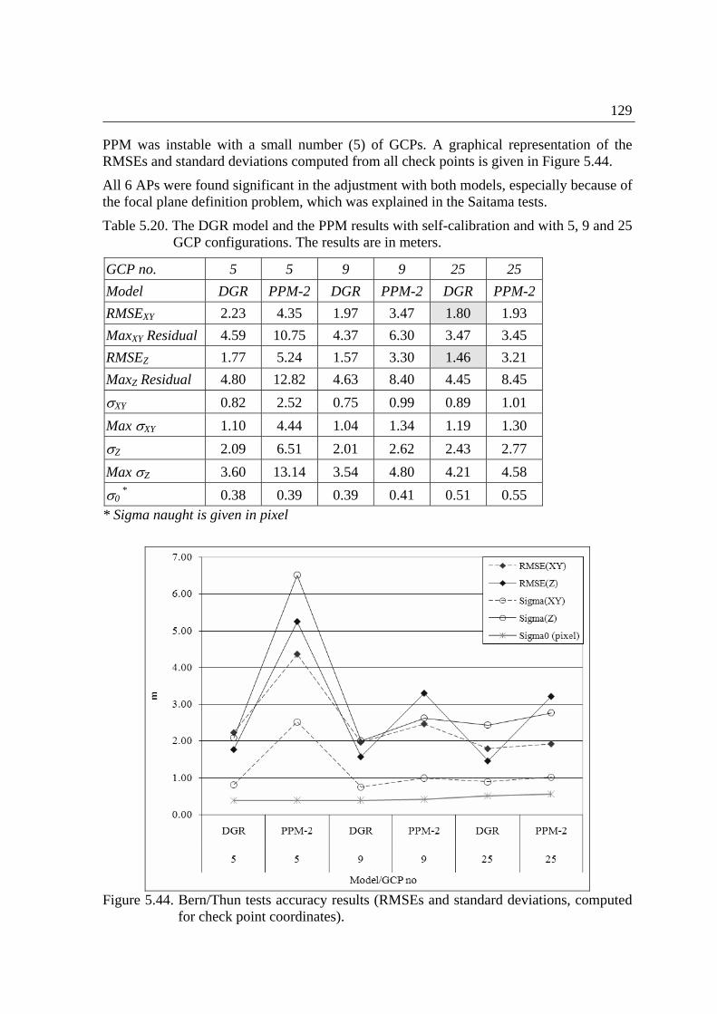
129

PPM was instable with a small number (5) of GCPs. A graphical representation of the RMSEs and standard deviations computed from all check points is given in Figure 5.44.

All 6 APs were found significant in the adjustment with both models, especially because of the focal plane definition problem, which was explained in the Saitama tests.

Table 5.20. The DGR model and the PPM results with self-calibration and with 5, 9 and 25 GCP configurations. The results are in meters.

GCP no. 5 5 9 9 25 25

Model DGR PPM-2 DGR PPM-2 DGR PPM-2

RMSEXY 2.23 4.35 1.97 3.47 1.80 1.93

MaxXY Residual 4.59 10.75 4.37 6.30 3.47 3.45

RMSEZ 1.77 5.24 1.57 3.30 1.46 3.21

MaxZ Residual 4.80 12.82 4.63 8.40 4.45 8.45

XY 0.82 2.52 0.75 0.99 0.89 1.01

Max XY 1.10 4.44 1.04 1.34 1.19 1.30

Z 2.09 6.51 2.01 2.62 2.43 2.77

Max Z 3.60 13.14 3.54 4.80 4.21 4.58

0 *

0.38 0.39 0.39 0.41 0.51 0.55 * Sigma naught is given in pixel

Figure 5.44. Bern/Thun tests accuracy results (RMSEs and standard deviations, computed

for check point coordinates).

130

5.3.2.3 Piemont, Italy

The Piemont testfield is located in the north western part of Italy. The testfield was set up by GAEL Consultant, France. Due to mountainous terrain structure, it was difficult locate GCPs with a homogeneous distribution. The ground coordinates of the GCPs were determined by GPS. The main parameters of the PRISM dataset acquired over the Piemont testfield are given in Table 5.21. The GCPs are measured manually in the images. GCP distribution in PRISM nadir image is given in Figure 5.45.

Although the attitude data were provided for this dataset, they could not be employed in the adjustment. The main reason was the complexity of the data transformation between different coordinate systems and the lack of proper format definition. The a priori standard deviations of the unknown parameters in the adjustment, which were used to compute the weight coefficients, are similar to those of the Saitama dataset (Table 5.17).

Table 5.21. The main parameters of the PRISM dataset acquired over the Piemont testfield

Imaging Date 04.09.2006

Number of PRISM images 1 scene with forward, nadir and backward images

Viewing angles -23.8, 0, 23.8 Total no. of GCPs 29

Total no. of tie points 142 Since there are only 29 GCPs in the testfield, the DGR model and the PPM have been tested with two different GCP configurations. The results are given in Table 5.22 and a graphical representation is shown in Figure 5.46. The accuracy values are at sub-pixel level for all models. The DGR model performs again better than the PPM in the 5 GCPs configuration. The difference can be observed especially in the theoretical values. Similar to the Saitama and the Bern/Thun datasets, all APs were significant here in both models, especially due to focal plane definition problem.

Table 5.22. The DGR model and the PPM results with self-calibration and with 5 and 9 GCP configurations. The results are in meters.

GCP no. 5 5 9 9

Model DGR PPM-2 DGR PPM-2

RMSEXY 2.34 2.58 2.22 2.20

MaxXY Residual 3.71 4.10 3.55 4.19

RMSEZ 1.05 2.36 1.03 1.20

MaxZ Residual 2.36 4.84 2.04 2.18

XY 0.58 2.37 0.59 0.68

Max XY 0.67 6.66 0.70 1.40

Z 1.60 4.10 1.64 1.82

Max Z 1.84 10.68 1.94 3.23

0 *

0.28 0.26 0.30 0.27 * Sigma naught is given in pixel

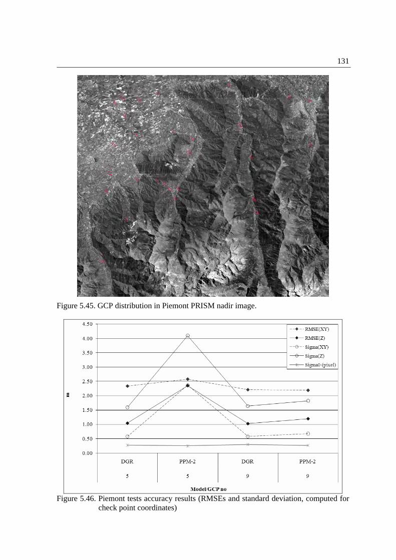
131

Figure 5.45. GCP distribution in Piemont PRISM nadir image.

Figure 5.46. Piemont tests accuracy results (RMSEs and standard deviation, computed for

check point coordinates)

132

5.3.2.4 Okazaki, Japan

The Okazaki testfield is located in the Aichi Prefecture on the Honshu island of Japan. The testfield has been generated as the 2nd ALOS/PRISM Cal/Val dataset by JAXA. The main project parameters are given in Table 5.23. GCP distribution in the PRISM nadir image is shown in Figure 5.47. The attitude data were provided for this dataset. However, this data could not be employed in the adjustment due to missing transformation parameters in the algorithm. The a priori standard deviations of the unknown parameters in the adjustment are defined similar to those of the Saitama dataset (Table 5.17).

Table 5.23. Main parameters of the PRISM dataset acquired over the Okazaki testfield.

Imaging Date 20.06.2006

Number of PRISM images 1 image triplet

Viewing angles -23.8, 0, 23.8 Total number of GCPs 51

No. of tie points 135

Figure 5.47. GCP distribution in Okazaki PRISM nadir image.

133

The DGR results with 5, 9, and 25 GCP configurations and the PPM results with 25 GCPs are presented in Figure 5.48. Since the Okazaki tests were performed after the first three testfields, the PPM was not applied with a small number of GCPs. Only the 25 GCPs configuration is used and the whole trajectory is modeled with one segment only.

0.00

0.50

1.00

1.50

2.00

2.50

3.00

3.50

DGR DGR DGR PPM-1

5 9 25 25

Model/GCP no.

m

RMSE(XY)

RMSE(Z)

Sigma(XY)

Sigma(Z)

Sigma0 (pixel)

Figure 5.48. Okazaki tests accuracy results (RMSEs and standard deviations, computed for check point coordinates)

Using the DGR model, there was not much to gain from 5 to 25 GCPs in planimetric accuracy. However, the height accuracy improved with the increase of the number of GCPs. The a posteriori sigma naught values were very similar in all tests and vary between 0.51-0.54 pixels. Comparing the results of the DGR and the PPM test, the theoretical and empirical accuracy values are equally the same. From these tests, it can be again concluded that the DGR parameters are sufficient to model the trajectory errors.

Considering the 25 GCPs tests, the AP significance patterns were similar in both models. Scale parameters in forward and nadir images, and the CCD line bending parameter in backward image were found significant in the Student’s test.

134

5.3.2.5 Zurich, Switzerland

The Zurich/Winterthur testfield has been established by the IGP, ETH Zurich in summer 2007 under an ESA-ESRIN contract. The PRISM image triplet has been acquired before the establishment of the testfield. During the GPS measurement campaign, the images were used to select the control points with good image definition. The main parameters of the PRISM dataset in this testfield are given in Table 5.24. A total of 99 GCPs were measured in the field and also in the PRISM images. The GCPs and the tie points were measured with least squares matching. However, the matching procedure was not successful for some of the points due to inferior image definition and these points have been measured manually. The testfield setup is represented in Figure 5.49. The overview and the documentations of the GCP’s are reproduced with authorization of Swisstopo, Switzerland (ref: BA081107).

Table 5.24. Main parameters of the PRISM dataset acquired over the Zurich/Winterthur testfield

Imaging date 22.04.2007

Number of PRISM images 1 image triplet

Viewing angles (nominal) -23.8, 0, 23.8 Total no. of GCPs 99

No. of tie points 101

Before testing the Zurich/Winterthur data, the coordinate system transformation algorithm of the software was improved using an updated format description. However, the task could not be accomplished, again due to partially missing information. Therefore, the complete coordinate transformation parameters were not employed in the model. The calibration data of the sensor relative alignment parameters were still missing in the transformation, which introduced a constant shift error into the position and attitude parameters in the adjustment. The drift error in the attitude data could be removed with the new implementation.

The positional shift values were relatively small (below 2 m). Considering the accuracy of given position data (usually given as 1 m) and the spatial resolution of the sensor, their effect can be neglected in the error budget.

3 attitude shift parameters (roll, pitch, and yaw) per image trajectory were estimated in the adjustment, with 0.07 a priori standard deviation. This value is quite small in comparison to the former datasets, where the trajectory attitude data was not provided and/or employed. The complete weighting schema is provided in Table 5.25.

The dataset was tested with the DGR and the PPM model with one segment per image trajectory. With the help of more accurate trajectory data, smaller number of GCPs could be tested for this dataset. 1, 2, 4, and 9 GCP configurations have been used in the tests. The points were selected in a homogeneous distribution in planimetry for the multiple GCP cases. The results are provided in Table 5.26 and Figure 5.50.

135

Figure 5.49. The Zurich/Winterthur testfield configuration. The red dots represent the GCP locations, the blue rectangle represents the border of the PRISM nadir image, and the yellow rectangles denote the coverage areas of two reference DSMs.

Table 5.25. A priori standard deviations used for the unknown parameters of the Zurich/Winterthur PRISM dataset.

Parameter Std. deviations () in DGR Std. deviations () in PPM

Xoff, Yoff, Zoff 2 m 2 m (X0, Y0, Z0)

X1, Y1, Z1 Not applicable 1 m

X2, Y2, Z2 Not applicable 0.5 m

0, 0, 0 0.07 0.07

1, 1, 1 0.0001 0.0001

2, 2, 2 Not applicable 0.00001

GCP (X,Y,Z) 20 cm

Image measurement 0.5 pixels

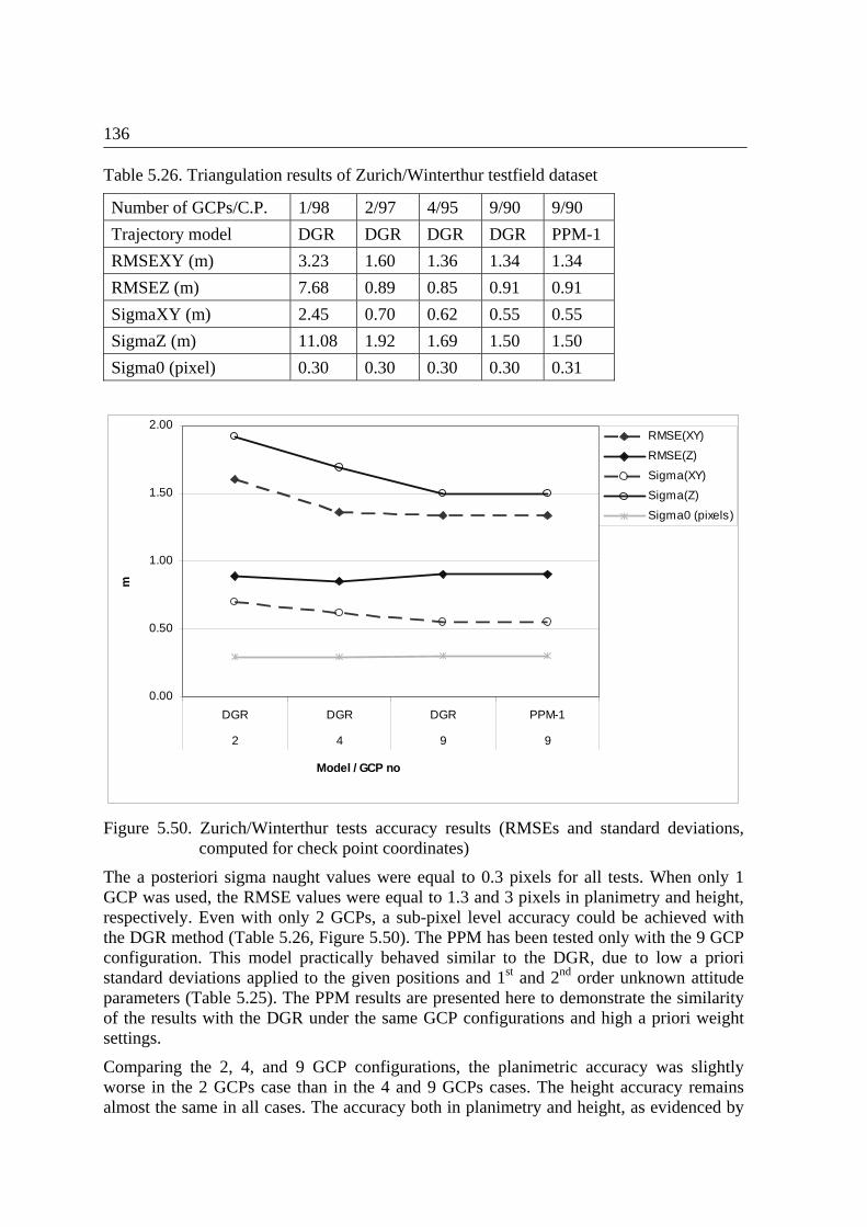
136

Table 5.26. Triangulation results of Zurich/Winterthur testfield dataset

Number of GCPs/C.P. 1/98 2/97 4/95 9/90 9/90

Trajectory model DGR DGR DGR DGR PPM-1

RMSEXY (m) 3.23 1.60 1.36 1.34 1.34

RMSEZ (m) 7.68 0.89 0.85 0.91 0.91

SigmaXY (m) 2.45 0.70 0.62 0.55 0.55

SigmaZ (m) 11.08 1.92 1.69 1.50 1.50

Sigma0 (pixel) 0.30 0.30 0.30 0.30 0.31

0.00

0.50

1.00

1.50

2.00

DGR DGR DGR PPM-1

2 4 9 9

Model / GCP no

m

RMSE(XY)

RMSE(Z)

Sigma(XY)

Sigma(Z)

Sigma0 (pixels)

Figure 5.50. Zurich/Winterthur tests accuracy results (RMSEs and standard deviations, computed for check point coordinates)

The a posteriori sigma naught values were equal to 0.3 pixels for all tests. When only 1 GCP was used, the RMSE values were equal to 1.3 and 3 pixels in planimetry and height, respectively. Even with only 2 GCPs, a sub-pixel level accuracy could be achieved with the DGR method (Table 5.26, Figure 5.50). The PPM has been tested only with the 9 GCP configuration. This model practically behaved similar to the DGR, due to low a priori standard deviations applied to the given positions and 1st and 2nd order unknown attitude parameters (Table 5.25). The PPM results are presented here to demonstrate the similarity of the results with the DGR under the same GCP configurations and high a priori weight settings.

Comparing the 2, 4, and 9 GCP configurations, the planimetric accuracy was slightly worse in the 2 GCPs case than in the 4 and 9 GCPs cases. The height accuracy remains almost the same in all cases. The accuracy both in planimetry and height, as evidenced by

137

RMSEXY and RMSEZ, was below one pixel in all tests. The PPM results were the same as the DGR model results of the same 9 GCP configuration.

Considering the self-calibration, four of the additional parameters (scale parameters of the forward-nadir-backward images and the CCD line bending parameter of the nadir image) were statistically significant in the Zurich/Winterthur tests.

5.3.3 Findings and Discussion

The calibration procedure of the ALOS/PRISM images is presented here in a chronological order. The software and algorithm development steps have been carried out using testfield data acquired over five areas. The Piemont, Italy, Saitama and Okazaki, Japan and Bern/Thun, Switzerland, datasets represent earlier phases of the images and also algorithms. The Zurich/Winterthur testfield was setup later and the most recent PRISM data were acquired over this testfield. PRISM images from a number of other testfields have been tested afterwards, but the results were quite similar and they are discussed in Kocaman and Gruen (2008).

Here, the PRISM system has been calibrated using the technique of self-calibration. In all cases, PRISM image triplets have been used. Validation is a system approach. It includes the sensor performance, but also the quality of both the data processing algorithms and the reference data. The validations of our georeferencing procedures could be performed in all five testfields.

We started our calibration approach with partially uncalibrated Saitama image data. The missing information concerning the precise location of the individual focal plane array CCD chips with respect to the camera’s principal point led to significant systematic errors in object and image space. By applying the respective additional parameters in our self-calibration procedure (2 shifts for each chip in image space) we were able to compensate these systematic errors, thus leading to much better results (improvement of up to 50%).

After receiving from JAXA the calibrated shift values for the chips we applied those and found the results correct after validation by self-calibration.

For georeferencing we applied both our sensor/trajectory models DGR and PPM and found that DGR had the better performance in case of very few GCPs. Under the given sensor configurations the PPM method turned out to be a bit instable with 5 GCPs, but with 9 and more GCPs both methods performed equally well overall.

Considering the DGR results only, a brief summary of the accuracy values obtained in the best GCP configurations over all five testfields are summarized in Table 5.27. Concerning the planimetric accuracy the theoretical expectations (SigmaXY) were usually significantly better than the empirical values (RMSEXY). However, we note that in some cases the empirical height accuracy values (RMSEZ) were even better than the corresponding theoretical precision values. This can be explained by the fact that the image definitions of the points in planimetry were much worse than the height definition. This problem arises basically from the image radiometric quality problems. On the other hand, the GCPs were defined mostly on the road intersections, which can usually be considered as flat in the area of one pixel.

138

Table 5.27. Summary of the accuracy results obtained from the best GCP and sensor model configurations in all 5 testfields

Component Parameter Minimum (m) Maximum (m)

RMSE XY 1.20 2.30 Planimetric accuracy Sigma XY 0.55 0.94

RMSE Z 0.85 2.50 Height accuracy

Sigma Z 1.50 2.60

Sigma 0 0.27 0.54

Over all five testfields we achieved with our empirical accuracy values quite consistent results. We stay in all cases in the sub-pixel domain, in the best cases we achieved about half a pixel planimetric accuracy and 1/3 pixel height accuracy. This relatively high accuracy is surprising, considering the fact that the image quality of PRISM has still much potential for improvement. On the other side one usually uses only well defined points as GCPs and check points, where the inferior image quality has not such a negative influence.

With the latest version of the algorithm, which was developed during this study, and the calibration data provided by JAXA, two GCPs are sufficient to model the errors of the system and to calibrate the images.

Self-calibration is a very powerful method for sensor model refinement. However, it should be noted that the most appropriate additional parameter functions have not yet been fully explored for PRISM imagery. The physical sensor model is still not complete due partially missing relative alignment parameters in the coordinate system transformation. In any case, self-calibration should be used with great care. The statistical testing of additional parameters for determinability is a crucial requirement for a successful use of this technique.

If we compare these georeferencing results with those which were obtained with other satellite sensors of similar type (SPOT-5, IKONOS, Quickbird, Cartosat-1) we note that the accuracy (expressed in pixels) is about the same as with these other sensors.

6

CONCLUSIONS and OUTLOOK

6.1 Summary

This study has accomplished a large part of the initial objectives. Sensor geometries and self-calibration capabilities of a number of aerial and satellite Linear Array CCD sensors have been investigated under different network conditions, i.e. different numbers of strips, images, GCPs, etc. However, systematic studies with synthetic data are still required in order to provide definitive conclusions.

Imagery of a number of aerial and satellite Linear Array CCD sensors have been oriented using rigorous models based on collinearity conditions. The Linear Array Bundle adjustment software developed at the IGP, ETH Zurich, has been adapted according to the requirements of each sensor. In addition, algorithms for the preparation of image datasets for the sensor orientation have been implemented in the software. Among those, image and trajectory extraction, coordinate transformations between coordinate systems (object spaces, image space, and pixel space), preprocessing of calibration data can be listed. For reference data preparation, GCP coordinate measurements were performed in the images and on the ground. Additional tie points were extracted manually or semi-automatically when needed.

Three different trajectory models were used for the investigations. The Direct Georeferencing Model (DGR) is the relatively simple one among all three considering the mathematical model and the number of unknown parameters introduced into the adjustment. In this study, the model has been applied to both aerial and satellite cases. The Lagrange Interpolation Model (LIM) has been preferred for the modeling of the imagery of the aerial Linear Array CCD sensors, while the Piecewise Polynomial Model (PPM) has been applied only in the satellite images, where the satellite moves along a smoother trajectory and a small number of segments is sufficient for modeling. With LIM, at least four orientation fixes should be defined with the current implementation of the model.

140

The self-calibration is a useful technique for on-the-job calibration of sensors and modeling of the system errors and thus improving the accuracies in practical applications. It has been applied to the data of all sensors used in this study. Different additional parameter sets have been defined for the airborne and satellite cases due to differences between focal plane arrangements and the sensor characteristics. In both cases, the self-calibration has been found useful when applied with appropriate care.

Images of two different aerial Linear Array CCD sensors, the STARIMAGER of former Starlabo Corporation, Japan, and the ADS40 sensor of the Leica Geosystems, Heerbrugg, were used for the investigations. The results obtained from two different engineering models of STARIMAGER, the SI-100 and the SI290 models, are presented here. The images were acquired over the Yoriichio Testfield, Japan. A number of image and trajectory problems have been encountered in the dataset, which resulted in relatively low georeferencing accuracy and requirement of a large number of GCPs. On the contrary, both of the ADS40 datasets, which were acquired over the Vaihingen/Enz Testfield, Germany, and the Pavia Testfield, Italy, have superior quality in terms of image and trajectory data. All practical results are presented in Chapter 5 of this report.

Briefly, the main achievements of the STARIMAGER datasets are:

Considering the Yoriichio SI-290 dataset and the three different block configurations, the best accuracy results were obtained with the LIM. The results were between 1.1-1.6 pixels in planimetry and 2.1-3.3 pixels in height. The best results were obtained using the highest number of GCPs, which was 11 for the single strip and 20 for the multiple strips cases. With the cross-strip configuration of 4-strips, it was possible to obtain a relatively stable system even with 3 control points. The Single strip tests have shown that the single strip has poor geometry and use of a higher number of GCPs was necessary. In this dataset, an efficient block configuration provided a better handling of correlations between the EO parameters and high accuracy with small number of GCP.

Considering the SI-100 Yoriichio dataset, the APs have improved the overall system accuracy. In the best case with the LIM and 30 orientation fixes, and using 30 GCPs, the RMSE values corresponded to 1 pixel in planimetry and 2 pixels in height.

Both datasets cope with poor image quality, small ground signal size, and problems in GPS/INS processing. The trajectory data used in these tests have most probably a high noise level. The DGR was not adequate to model these errors. Therefore, the trajectory modeling with the LIM was very important for a high adjustment accuracy. However, with the small number of control points (<=6), it was better to use the DGR model or the LIM with smaller number of orientation fixes (4-6 fixes, depending on the GCP distribution).

Major achievements of the ADS40 datasets were:

The Vaihingen/Enz block has outstanding trajectory accuracy, especially in height. The RMSE values achieved with 4, 9, and 12 GCPs did not show significant differences. The use of self-calibration improved the RMSEs only in planimetry. Without considering the improvement of the GSD with the use of staggered array technology, the best RMSE values obtained in this dataset were 0.21-0.37 pixels in

141

planimetry and in height, respectively. These results were obtained with the DGR and with self-calibration. The modeling of the trajectory with LIM was not necessary in this case.

In the Pavia ADS40 tests, we had the possibility to compare our results with the University of Pavia results. The direct georeferencing results were identical in terms of RMSE values. The 2000 m dataset provides a good level of accuracy, 0.5 pixels in planimetry and 3 pixels in height, even without the use of GCPs. The direct georeferencing results of the 4000 m block were worse and resulted in 1.2 pixels in planimetry and 4.6 pixels in height with a forward intersection. The bundle adjustment results were comparable to the University of Pavia results when the self-calibration was applied. For the 2000 m block, the best RMSE values were 0.2 and 0.25 pixels in planimetry and height, respectively. For the 4000 m block, using the DGR with 5 GCPs and with self-calibration, the RMSE values resulted in 0.2 and 0.3 pixels in planimetry and in height, respectively. The use of self-calibration improved the accuracy in all cases. We should also note that the staggered array technology was switched off during the Pavia test flights.

Overall, the ADS40 tests showed that the APs are in general determinable under given estimation model parameters. No high disturbances on the object point coordinates caused by the APs were observed in the trace check algorithm. Our parameter removal algorithm works efficiently. An accurate image and trajectory dataset can reach the geometric accuracy potential even with few well-defined GCPs.

The PRISM onboard of the Japanese ALOS is the example of the satellite Linear Array CCD sensor used for investigations in this study. PRISM can acquire along-track image triplets with multiple camera heads. 12 different PRISM image datasets acquired over designated testfields have been georeferenced and calibrated. The results of only the first five datasets are presented here due to two reasons. First, the early PRISM datasets reflect the calibration problems, which had been faced in the initial period after the satellite launch. Second, the sensor is already geometrically calibrated and stable, and has reached its accuracy potential in terms of georeferencing. The recent PRISM datasets (i.e. Adana, Turkey, Wellington, South Africa, Sakurajima, Japan, Haiphong, Vietnam, Thimpu, Bhutan) have similar accuracy with the presented datasets and do not exhibit any new characteristics.

The Piemont, Italy, Saitama and Okazaki, Japan, and Bern/Thun, Switzerland, datasets represent the earlier phases of image acquisition and calibration, data processing, and algorithm development both at the IGP and at JAXA. The more recent PRISM images were acquired over the Zurich/Winterthur testfield. Dense and homogeneous GCP distribution in the PRISM images were provided in this testfield. PRISM Level 1B1 (geometrically uncorrected) image triplets have been used in all testfields. The results of the five datasets can be summarized as:

Self-calibration is powerful to model the systematic errors of the PRISM images. In the early steps of the Saitama processing, the missing information concerning the precise location of the individual focal plane array CCD chips with respect to the camera’s principal point led to significant systematic errors in object and image space. By applying the respective additional parameters in our self-calibration

142

procedure, we were able to compensate these systematic errors, and achieve much better results (improvement of up to 50%). After receiving the calibrated shift values of the CCD chips from JAXA, we have performed the adjustment again and validated the values by self-calibration.

For georeferencing we have applied two of our sensor/trajectory models, the DGR and the PPM, and found that the DGR performed better in case of very few GCPs. The PPM method turned out to be a bit instable with small number of GCPs. But with 9 and more GCPs, both methods performed equally accurate overall. Considering the DGR results only, the best RMSE values, which were achieved in over all five testfields, are between 1.2-2.3 pixels in planimetry and 0.85-2.5 pixels in height.

If we compare these georeferencing results with those which were obtained with other satellite sensors of similar type (i.e. SPOT-5, IKONOS, Quickbird, Cartosat-1, etc.), we see that the accuracies (expressed in pixels) are almost the same.

6.2 Conclusions

Overall, the following points and conclusions can be highlighted for all sensors and datasets:

A number of well defined points as GCPs and check points are necessary for comprehensive analysis of the systems’ geometries and self-calibration capabilities. The minimum number of GCPs required for this procedure depends mainly on:

- sensor configuration (i.e. number of lenses and Linear Array CCDs),

- image block configuration (e.g. the number of image strips and the number of images per strip),

- quality of the given trajectory and the camera calibration data,

- selected trajectory model and its configuration in the bundle adjustment,

- and, use of self-calibration and the definition of additional parameters,

The GCP ground coordinates are nowadays measured with differential GPS technology and the measurement accuracy is adequate for the use of large format aerial digital cameras and high-resolution satellite optical sensors. Definition of GCPs in images is a key issue for accurate sensor orientation and can sometimes be a limiting factor for high-accuracy due to low image quality and signalization problems on the ground. A homogeneous distribution of the GCPs should be considered while preparing a calibration and validation test site. Full planimetric and vertical coverage of the image extent should be aimed at.

Depending on the number of control and check points, the use of tie points might be necessary when a complex trajectory model (such as the PPM or the LIM), and self-calibration are used in the adjustment. In addition, the minimum number of tie points depends also on the number of orientation fixes defined for the LIM and number of segments defined for the PPM.

143

As can be seen from the STARIMAGER applications, the point determination accuracy of the Linear Array CCD sensors is highly dependent on the quality of the given trajectory. If the trajectory data contains large systematic errors, trajectory modeling in the adjustment using the PPM or LIM is crucial. The main drawback of these models is the requirement for a high number of GCPs. Using accurate a priori trajectory data, the systematic error correction with the DGR is usually sufficient and a small number of GCPs (between 2-6, depending on the AP set) is enough in these cases.

Another advantage of high quality trajectory data appears in the handling of the stochastical model. The EO parameters of the Linear Array CCD imagery are highly correlated (especially between X- and Y-). The correlation pattern weakens the system, may reduce the adjustment reliability and parameter determinability for the EO parameters and the APs in general, and increases the demand for a higher number of GCPs. Therefore, the operational aspects of the Linear Array CCD image acquisition and data preprocessing (i.e. trajectory data processing with Kalman Filtering) become much more important than the traditional film imaging and the Matrix Array imagery.

The self-calibration is applicable to the Linear Array CCD imagery. Our experiences have shown that the success of the self-calibration depends mainly on:

- the mathematical definition of APs,

- sensor configuration (i.e. number of lenses and Linear Array CCDs),

- test site configuration (e.g. the number of image strips and the number of images per strip, the number and the distribution of the GCPs, etc.),

- quality of the given trajectory and the camera calibration data,

- selected trajectory model and its configuration in the bundle adjustment,

- existence of systematic errors in the system,

- and, the noise level contained in the system.

The applications of the self-calibration to the STARIMAGER datasets were the problematic cases, mainly due to the trajectory errors and other undefined errors of the system, and also low image quality of the GCPs. The parameter definition and determinability are the key issues of self-calibration and the method should not be applied blindly. The AP sets for each sensor should be tested and analyzed comprehensively using the imagery acquired over well-defined testfields. Accurate reference data is necessary for validation of the methods and the image data. Using appropriate statistical detection tools, parameter determinability should be checked at different steps of the adjustment.

The data snooping algorithm of Baarda was tested with different trajectory models and image datasets. The method has worked efficiently to detect blunders in the image measurements and provided a testing with clear datasets (free of gross errors).

144

6.3 Recommendations and Future Work

In order to understand the systems fully, more investigations on the Linear Array CCD imagery should be performed. The applications presented here can be seen as early steps of this research field. Further work is necessary, especially on:

i. Trajectory analysis methods, in order to understand the quality of given image trajectory data,

ii. Analysis of the stochastical model, sensitiveness of the models to given apriori accuracies of GCPs and the trajectory data,

iii. Extension of the investigations on the trajectory models and the self-calibration for other Linear Array CCD sensors,

iv. Investigations on the direct georeferencing capabilities of the sensors (so far, only the accuracies of the ADS40 datasets could be assessed with direct georeferencing).

v. And, structural analysis on the trajectory models and the network conditions using synthetic data.

Investigations with synthetic data are recommended as a part of the future work also for realization of the first two items above. Although systematic investigations with synthetic data were part of the objectives of this study at the beginning and was even initiated for the airborne Linear Array CCD imagery (Kocaman and Gruen, 2006), it was not possible to finalize this part of the work within the time frame.

The most time consuming aspects of working with the practical data came from the metadata extraction and data import to the software format. Currently, the fields of aerial and satellite photogrammetry lack standardization of data processing methods and presentation to the users. There is a variety of sensor orientation and calibration methods; yet the society does not have a consensus on the processing methods of Linear Array CCD imagery. In addition, the image and the auxiliary data are usually presented in different formats by the image vendors, creating difficulties in importing the data into existing software and algorithms. A standardization of the formats and methods would increase the speed of any research work and software development in these fields and provide the users better understanding of the systems.

APPENDIX

FUNDAMENTALS OF FRAME BUNDLE ADJUSTMENT

A.1 Introduction to the Least Squares Estimation

Most of the quantities involved in photogrammetric processes are random variables. Their values are obtained from measurements. Due to several factors, such as human limitations, instrumental imperfections, there is a certain amount of errors included in the measurements. An error is the difference between an observed value of a variable and its true value. The errors are categorized as random errors, systematic errors, and gross errors (blunders).

The blunders and systematic errors in the measurements can be eliminated with appropriate care and mathematical corrections. However, the random errors cannot be corrected and are treated with a statistical method, called least squares adjustment. The method was introduced by Carl Gauss at the beginning of 19th century.

The least squares adjustment assumes that the measurements are redundant, so that there are more measurements than the number of unknowns in the adjustment. The redundancy is denoted as:

r= n-u; n>u

where n is the number of measurements and u is the number of unknowns. r is known also as degrees of freedom in the adjustment.

The number of unknowns is defined according to the mathematical model used. The mathematical model describes the geometric and physical situation involved in the adjustment problem. The mathematical model is composed of two parts: a functional model and a stochastical model. When the sensor orientation problem is considered, the functional model is determined by the chosen georeferencing method. The stochastical

(A.1)

146

model includes the a priori knowledge about the accuracy of the measured quantities, which are introduced with weights in the adjustment.

In the least squares adjustment, the true value, which is theoretically the correct or exact value of a variable cannot be obtained. Instead, the most probable value, which has the highest probability for a measured or indirectly determined quantity, is estimated based on the observations. The observations are the directly measured/observed quantities and contain random errors.

A.1.1 Method of Least Squares

A sensible method of estimating unknown parameters is given by minimizing the sum of the squares of the deviations of the observations l from the estimators s[E(l)] of their expected values E(l), which are functions of the unknown parameters (Koch, 1999). Let the linear model be:

l=Ax+e

where

s(E(l)) = Ax,

E(l)=l,

E(e)=0

l is the vector of observations, A is the coefficient matrix, x is the unknown parameters vector, and e is the vector of errors.

The method of least squares estimation (called also as least squares adjustment) aims at:

(l-Ax)T(l-Ax) = minimum

Since the vector of the true errors e is unknown, the vector of the residuals (v), which are the differences between an observed value and the value given by the model, is minimized in the estimation (v=-e).

A.1.2 Gauss-Markoff Model

Let A be an nu matrix of given coefficients, x a u1 vector of unknown, fixed parameters, l an n1 random vector of observations, and P(l)= 2 1D the nn covariance matrix of l, where the weight matrix D of observations l is known and the positive factor 2 is unknown. Let A have full column rank, i.e. rankA=u, and let the weight matrix P be positive definite. Then

Ax=E(l) with P(l)= 2 1D

(l-Ax)TP(l)-1(l-Ax) = minimum

(A.2)

(A.3)

(A.4)

(A.5)

147

is said to be a Gauss-Markoff model with full rank (Koch, 1999).

In this model, instead of minimizing the sum of squares of the residuals, one minimizes a quadratic form in the residuals. This leads to the estimator:

x = (ATPA)-1ATPl

which is the best linear unbiased estimator for x. The A is the design matrix in the adjustment, formed by observation equations, and P is the weight coefficient matrix of the l measurements vector.

The D(l)= 2 1P belongs to the stochastical part of the adjustment. It is assumed to be known except for the factor 2 . The matrix P is supposed to be positive definite and denotes the weight matrix of the observations l. In least squares adjustment, one also sets

1P =Q, which is the cofactors or weight coefficients matrix. The 2 is called the variance of unit weight (Koch, 1999). In practice, the unit weight (P0=I) is used for one type of observations. In bundle adjustment, the unit weight is usually used for the a priori standard deviation of the image coordinates:

0=img , P0=Pimg=I

where 20 corresponds to the 2 , the variance of the unit weight.

Weights of other observation equations are computed using following formulation:

02

20 PPi

i

where i is the a priori standard deviation of an observation i.

A.2 Statistical Testing (Hypothesis Testing)

Using the terminology of modern linear estimation theory for interval estimation, the linear adjustment model given in Equation (A.5) with the assigned weight matrix P can be formulated as a null-hypothesis H0 (Gruen, 1982):

H0: l N(Ax, 20 P-1)

(i.e. l has a multidimensional normal distribution with the assumptions as in Equation A.4). Suppose a minimum variance of unbiased estimates of x and 2

0 is performed with:

)ˆ()ˆ(1

ˆ 20 lxAPlxA

rT

where r is the redundancy given in Equation (A.1). The residuals are denoted by:

lxAv ˆ

(A.6)

(A.7)

(A.8)

(A.9)

(A.10)

(A11)

148

Under H0 the distributions of x and v are:

x N(x,Kxx), Kxx =20 Qxx

v N(0,Kvv), Kvv =20 Qvv

with the weight coefficients matrices:

Qxx = (ATPA)-1

Txxvv AAQPQ 1

The term precision is defined by the statistical features of the estimated parameters x , if the a priori assumptions (functional and stochastical relations) of the adjustment model are considered to be true. The covariance matrix Kxx contains all information concerning the precision of the solution x . The precision describes the deviation of the estimated x from its expectation associated with the corresponding model.

For the discussion of the effects of a possibly wrong model, the term accuracy becomes more important. The accuracy is formulated as:

A( x )=E(( x -x)( x -x)T)

If the adjustment model is a false model, then we get E(l)≠Ax. For more details on the model testing under the null-hypothesis of Equation (A.9), see Gruen (1982).

Another important aspect of the selected adjustment model is the reliability. The reliability defines the quality of the adjustment model with respect to the detection of model errors. Those errors can be blunders, systematic errors (errors in the functional assumptions), and weight errors (errors in the stochastical assumptions). Baarda’s (1967, 1968) reliability theory is a well-known and commonly used algorithm among photogrammetrists. The algorithm is based on the assumption that there is only one gross error in the observations at a time. The adjustment should be repeated to search for multiple errors. Using the elements (qvv) of Qvv given in Equation (A.15), the statistical test value wi for each observation is obtained as:

ivv

ii

q

vw

0

where vi is the corresponding element of the residual vector obtained by Equation (A.11), and 0 is the a priori sigma naught. According to a chosen significance level, a critical value |wmax| is compared with each wi. The internationally adopted significance level is 0.001 which has been chosen by Baarda (1968).

(A.13)

(A.15)

(A.17)

(A.12)

(A.14)

(A.16)

149

A.3 Frame Bundle Adjustment

The most elementary unit in photogrammetry is the image ray, which connects an object point, perspective center of an image, and the projection of the point on the image. The exterior orientation parameters, sensor interior geometry, and the systematic error components of the camera should be known to reconstruct the ray at the time of imaging.

A single frame image can be thought of as a bundle of such rays converging at the perspective center with an unknown position and orientation in space. A bundle block adjustment establishes the position and orientation of each bundle, using the rays in each bundle and the given ground control information (Mikhail et al., 2001). The bases of the bundle method are the collinearity equations:

jj

pjij

pjij

jij

Z

Y

X

c

yy

xx

R

Z

Y

X

00

where Xi, Yi, Zi are the object space coordinates of object point (Pi), X0j, Y0j, Z0j are the object space coordinates of the perspective center (Oj), xij, yij, 0 are the measured image coordinates of point ( '

ijP ), xpj, ypj are the image space coordinates of principal point (PPj), cj

is the camera constant for the lens j, Rj is the rotation matrix between image and object space coordinate systems, ij is the scale factor for the imaging ray. To relate the image coordinates (x, y) to the object coordinates (X, Y, Z) of a terrain point at any given instant, the collinearity equations are used.

The components of Equation (A.18) are reduced to two by canceling out the scale factor and are re-arranged according to:

xij = pjjijjijjij

jijjijjijj x

ZZrYYrXXr

ZZrYYrXXrc

)()()(

)()()(

033023013

031021011

yij = pjjijjijjij

jijjijjijj y

ZZrYYrXXr

ZZrYYrXXrc

)()()(

)()()(

033023013

032022012

r11j…r33j are the elements of the rotation matrix Rj. Three rotation angles (,,) are used to generate the rotation matrix. There are several methods to compute the elements. Here, the following formulations are used:

i

(A.18)

(A.19a)

(A.19b)

150

jjr coscos11

jjr sincos12

jr sin13

jjjjjr sincoscossinsin21

jjjjjr sincossinsinsin22

jjr sincos23

jjjjjr sinsincoscossin31

jjjjjr cossinsincossin32

jjr coscos33

Equations (A.19a) and (A.19b) can be written in compact form as:

xij = pj

z

xj x

f

fc

yij = pj

z

yj y

f

fc

(A.21a)

(A.21b)

(A.20)

BIBLIOGRAPHY Alamús, R., Kornus,W., Palà, V., Pérez, F., Arbiol, R., Bonet, R., Costa, J., Hernández, J.,

Marimon, J., Ortiz, M.A., Palma, E., Pla, M., Racero, S., Talaya, J., 2005. Validation process of the ICC digital camera. International Archives of Photogrammetry, Remote Sensing and Spatial Information Sciences, Vol. 36, Part I/W3 (on CD-ROM).

Alamús, R., Kornus, W., Talaya, J., 2006. Studies on DMC geometry. ISPRS Journal of Photogrammetry & Remote Sensing, Vol. 60, pp. 375–386.

Alhamlan, S., Mills, J.P., Walker, A.S., Saks, T., 2004. The influence of ground control points in the triangulation of Leica ADS40 data. Proceedings of the 20th ISPRS Congress, 12-23 July, Istanbul, International Archives of Photogrammetry, Remote Sensing and Spatial Information Sciences, Vol. 35 Part B1, pp. 495-500.

Atkinson, K.B. (Editor), 1996. Close range photogrammetry and machine vision. Whittles Publishing, Caithness, Scotland, 371 pages.

Baarda, W., 1967. Statistical concepts in geodesy. Netherlands Geodetic Commission, Vol. 2, No. 4, Delft, Netherlands, 74 pages.

Baarda, W., 1968. A testing procedure for use in geodetic networks. Netherlands Geodetic Commission, Vol. 2, No. 5, Delft, 97 pages.

Baltsavias, E. P., Stallmann, D., 1992. Metric information extraction from SPOT images and the role of polynomial mapping functions. International Archives of Photogrammetry, Remote Sensing and Spatial Information Sciences, Vol. 29, Part B4, pp. 358 - 364.

Baltsavias, E. P., Stallmann, D., 1996. Geometric potential of MOMS-02/D2 data for point positioning, DTM and orthoimage. International Archives of Photogrammetry, Remote Sensing and Spatial Information Sciences, Vol. 31, Part B4, pp. 110-116.

Baltsavias, E., Pateraki, M., Zhang, L., 2001. Radiometric and geometric evaluation of IKONOS Geo images and their use for 3D building modeling. Proceedings of the Joint ISPRS Workshop on "High Resolution Mapping from Space 2001", 19-21 September, Hannover, Germany (on CD-ROM).

152

Baltsavias, E., Kocaman, S., Akca, D., Wolff, K., 2007. Geometric and radiometric investigations of Cartosat-1 data. International Archives of Photogrammetry, Remote Sensing and Spatial Information Sciences, Vol. 36, Part I/W51 (on CD-ROM).

Baudoin, A. , Schroeder, M. , Valorge, C. , Bernard, M. , Rudowski, V., 2004. The HRS-Sap initiative: A scientific assessment of the High Resolution Stereoscopic Instrument on board of Spot-5 by ISPRS Investigators. Proceedings of the 20th ISPRS Congress, 12-23 July, Istanbul, International Archives of Photogrammetry, Remote Sensing and Spatial Information Sciences, Vol. 35, Part B1, pp. 372-378.

Becker, S., Haala, N., Reulke, R., 2005. Determination and resolution of spatial for digital aerial images. International Archives of Photogrammetry, Remote Sensing and Spatial Information Sciences, Vol. 36, Part I/W3 (on CD-ROM).

Beyer, H.A., 1992. Geometric and radiometric analysis of a CCD-camera based photogrammetric close-range system. Doctoral Thesis, No. 9701, Institute of Geodesy and Photogrammetry, ETH Zurich, Zurich, Switzerland.

Bodenstorfer, E., Fürtler, J., Brodersen, J., Mayer, K.J., Eckel, C., Gravogl, K., Nachtnebel, H., 2007. High-speed line-scan camera with digital time delay integration. Real-time image processing 2007, Editors: Nasser Kehtarnavaz and Matthias F. Carlsohn, Proceedings of the SPIE-IS&T Electronic Imaging, Vol. 6496, pp. 64960I, San Jose, California, U.S.A.

Boerner, A., Reulke, R., Scheele, M., Terzibaschian, Th., 1997. Stereo processing of Image data from an airborne three-line CCD scanner. The 3rd International Airborne Remote Sensing Conference and Exhibition, 7-10 July, Copenhagen, Denmark, Vol I, pp. 423-430.

Bouillon, A., Gigord, P., 2004. SPOT-5 HRS location performance tuning and monitoring principles. Proceedings of the 20th ISPRS Congress, 12-23 July, Istanbul, International Archives of Photogrammetry, Remote Sensing and Spatial Information Sciences, Vol. 35, Part B1, pp. 379-384.

Brown, D.C., 1971. Close-range camera calibration. Photogrammetric Engineering, Vol. 37 (8), pp. 855-866.

Brown, D.C., 1976. The bundle adjustment – progress and prospects. International Archives of Photogrammetry, Vol. 21(3), paper no 3-03-041, 33 pages.

Casella, V., Franzini, 2006. Presentation at the internal project meeting at the University of Pavia, Pavia, Italy, on 14.07.2006.

Casella, V., Franzini, M., Kocaman, S., Gruen, A., 2007a. Triangulation and self-calibration of the ADS40 imagery: a case study over the Pavia test site. Proceedings of the 8th Conference on “Optical 3D Measurement Techniques”, 9-12 July, Zurich, Switzerland, Vol. I, pp. 223-232.

Casella, V., Franzini, M., Padova, B., 2007b. Accuracy assessment of ADS40 imagery as a function of flying height and of aerial triangulation strategies. Proceedings of the 5th MMT Symposium, 29-31 May 2007, Padua, Italy (on CD-ROM).

153

Casella, V., Franzini, M., 2008. In-depth analysis of systematic errors in an ADS40 dataset. EuroCOW 2008 International Calibration and Orientation Workshop, Jan 30-Feb 1, Castelldefels, Spain (on CD-ROM).

Casella, V., Franzini, M., Kocaman, S., Gruen, A., 2008. Geometric accuracy assessment of ADS40 imagery under various network configurations. 21st ISPRS Congress, Beijing, China, 3-11 July, International Archives of Photogrammetry, Remote Sensing and Spatial Information Sciences, Vol. XXXVII. Part B1, pp. 627-632.

Chen, T., Shibasaki, R., Murai, S., 2003. Development and calibration of the airborne three-line scanner (TLS) imaging system. Photogrammetric Engineering & Remote Sensin, Vol. 69, no. 1, pp. 71-78.

Chen, T., Shibasaki, R., Tsuno, K., 2004. Orientation strategies of airborne three-line scanner STARIMAGER’s imagery with minimum ground control. Proceedings of the 20th ISPRS Congress, 12-23 July, Istanbul, International Archives of Photogrammetry, Remote Sensing and Spatial Information Sciences, Vol. 35 Part B3, pp. 36-40.

Clarke, T.A., Fryer, J.G., 1998. The development of camera calibration methods and models. The Photogrammetric Record, Vol. 16(91), pp.51-66.

Clarke, T.A., Fryer, J.G. and Wang, X., 1998. The principal point and CCD cameras. The Photogrammetric Record, Vol. 16(92), pp. 293-312.

Cramer, M., Stallmann, D., Haala, N., 1999. Sensor integration and calibration of digital airborne three-line camera systems. Proceedings of ISPRS Workshop Commission II/1 Mobile Mapping Technologies, 21-23 April, Bangkok, Thailand, International Archives of Photogrammetry, Remote Sensing and Spatial Information Sciences, Vol. 32, Part 2-5-3/W10.

Cramer, M., Stallmann, D., 2002. System calibration for direct georeferencing. ISPRS Commission III Symposium, Photogrammetric Computer Vision, 9-13 September 2002, Graz, Austria, International Archives of Photogrammetry, Remote Sensing and Spatial Information Sciences, Vol. 34 Part 3A, pp. 79-84.

Cramer, M., 2005. 10 years IFP test site Vaihingen/Enz: an independent performance study. Editor: Dieter Fritsch, Photogrammetric Week '05, Wichmann, Heidelberg, pp. 79-92.

Cramer, M., 2007. The EuroSDR performance test for digital aerial camera systems. Editor: Dieter Fritsch, Photogrammetric Week '07, 3-7 September, Stuttgart, Germany, pp. 89-106.

Doerstel, C., 2005. DMC – PPS and new features. Proceedings of ISPRS Workshop "High-Resolution Earth Imaging for Geospatial Information", 17-20 May, Hannover, Germany, International Archives of Photogrammetry, Remote Sensing and Spatial Information Sciences, Vol. 36, Part I/W3 (on CD-ROM).

Doerstel, C., Traub, S., Wuescher, D., 2005. Towards fully automated processing of DMC images. Proceedings of ISPRS Workshop High-Resolution Earth Imaging for Geospatial Information, 17-20 May, Hannover, Germany, International Archives of Photogrammetry, Remote Sensing and Spatial Information Sciences, Vol. 36, Part I/W3 (on CD-ROM).

154

Ebner, H., 1976. Self-calibrating block adjustment. International Archives of Photogrammetry, Vol. 21(3), paper no. 3-04, 17 pages.

Ebner, H., Kornus, W., Ohlhof, T., 1992. A simulation study on point determination for the MOMS-02/D2 space project using an extended functional model. International Archives of Photogrammetry, Remote Sensing and Spatial Information Sciences, Vol. 29, Part B4, pp. 458-464.

El-Manadili, Y., Novak, K., 1996. Precise rectification of SPOT imagery using the direct linear transformation model. Photogrammetric Engineering and Remote Sensing, Vol. 62(1), pp. 67-72.

Eisenbeiss, H., Baltsavias, E., Pateraki, M., Zhang, L., 2004. Potential of IKONOS and QuickBird imagery for accurate 3D point positioning, orthoimage and DSM generation. International Archives of Photogrammetry, Remote Sensing and Spatial Information Sciences, Vol. 35, Part B3, pp. 522-528.

Ethridge, M.M., 1977. Geometric analysis of singly and multiply scanned aircraft digital arrays. Ph.D. thesis, Purdue University, West Lafayatte, Indiana, 301 pages.

Fraser, C., S., Shao, J., 1996. Exterior orientation determination of MOMS-02 three-line imagery: experiences with the Australian test field data. International Archives of Photogrammetry, Remote Sensing and Spatial Information Sciences, Vol. 31, Part B3, Vienna, pp. 207-214.

Fraser, C.S., 1997. Digital camera self-calibration. ISPRS Journal of Photogrammetry and Remote Sensing, Vol. 52, pp. 149-159.

Fraser, C.S., Baltsavias, E., Gruen, A., 2001. IKONOS Geo stereo images: geometric potential and suitability for 3D building reconstruction. Photogrammetrie-Fernerkundung-Geoinformation: Geodaten schaffen Verbindungen, Vol. 10, pp. 113-121.

Fraser, C.S., Baltsavias, E., Gruen, A., 2002. Processing of IKONOS imagery for submetre 3D positioning and building extraction. ISPRS Journal of Photogrammetry and Remote Sensing, Vol. 56, pp. 177-194.

Fricker, P., 2001. ADS40 – progress in digital aerial data collection. Editors: D. Fritsch and R. Spiller, Photogrammetric Week 2001, Wichmann Verlag, Heidelberg, Germany, pp. 105-116.

Fritsch, D., 1997. Experiences with the airborne three-line camera system DPA. Photogrammetric Week’97, Wichmann Verlag, Eds. Fritsch/Hobbie, pp. 63-74.

Fritsch, D., Stallmann, D., 2000. Rigorous photogrammetric modeling processing of high resolution satellite imagery. International Archives of Photogrammetry, Remote Sensing and Spatial Information Sciences, Vol. 33, Part B1, pp.313-321.

Geoeye, 2008. GeoEye imagery products: IKONOS. http://www.geoeye.com/products/imagery/ikonos/default.htm (last accessed on 29.05.2008)

Grejner-Brzezinska, D.A., Toth, C.K., 1998. GPS error modeling and OTF ambiguity resolution for high-accuracy GPS/INS integrated system. Journal of Geodesy, vol. 72, pp. 626-638.

155

Grejner-Brzezinska, D.A., 1999. Direct exterior orientation of airborne imagery with GPS/INS system: performance analysis. Navigation, Vol. 46, No. 4, pp. 261-270.

Grewal, M.S., Weill, L.R., Andrews, A.P., 2001. Global positioning systems, inertial navigation, and integration. John Wiley and Sons Publication, New York, U.S.A.

Grodecki, J., Dial, G., 2003. Block adjustment of high-resolution satellite images described by rational polynomials. Photogrammetric Engineering & Remote Sensing, Vol. 69(1), pp. 59-68.

Gruen, A., 1978. Progress in photogrammetric point determination by compensation of systematic errors and detection of gross errors. Nachrichten aus dem Karten- und Vermessungswesen, Series II, 36, 113-140.

Gruen, A., 1982. The accuracy potential of the modern bundle block adjustment in aerial photogrammetry. Photogrammetric Engineering & Remote Sensing, Vol. 48, No. 1, pp. 45-54

Gruen, A., 1985a. Data processing methods for amateur photographs. The Photogrammetric Record, Vol. 11 (65), pp. 567-579.

Gruen, A., 1985b. Algorithmic aspects in on-line triangulation. Photogrammetric Engineering & Remote Sensing, Vol. 51, No. 4, pp. 419-436.

Gruen, A., Beyer, H.A., 2001. System calibration through self-calibration. Calibration and Sensor Orientation of Cameras in Computer Vision, Editors: Gruen and Huang, Springer-Verlag Berlin, Heidelberg, pp.163-193.

Gruen, A., Zhang, L., 2002. Sensor modelling for aerial mobile mapping with Three-line Scanner (TLS) imagery. Symposium of ISPRS Commission II, "Integrated System for Spatial Data Production, Custodian and Decision Support", 20-23 August, Xian, China, International Archives of Photogrammetry, Remote Sensing and Spatial Information Sciences, Vol. 34, part 2, pp. 139-146.

Gruen, A., Zhang, L., 2003. Sensor modeling for aerial triangulation with Three-Line-Scanner (TLS) imagery. Journal of Photogrammetrie, Fernerkundung, Geoinformation, Vol. 2, pp. 85-98.

Gruen, A., Eisenbeiss, H., Hanusch, T., Sauerbier, M., Wolff K., 2006. Documentation of the reference DSMs of the ALOS testfield Bern/Thun, Switzerland. Report to JAXA, Japan.

Gruen, A., Kocaman, S., Wolff, K., 2007. Calibration and validation of early ALOS/PRISM images. The Journal of the Japan Society of Photogrammetry and Remote Sensing, Vol 46, No. 1, pp. 24-38.

Gruen, A., Wolff, K., 2007. DSM Generation with ALOS/PRISM Data Using SAT-PP. IEEE International Geoscience and Remote Sensing Symposium (IGARSS) 2007, July 23 -27 (on CD-ROM).

Haala, N., Stallmann, D., Cramer, M., 1998. Calibration of directly measured position and attitude by aerotriangulation of three-line airborne imagery. International Archives of Photogrammetry and Remote Sensing, Vol. 32, Part 3, pp. 23-30.

156

Haala, N., Fritsch, D., Stallmann, D., Cramer, M., 2000. On the performance of digital airborne pushbroom cameras for photogrammetric data processing – a case study. International Archives of Photogrammetry and Remote Sensing, Vol. 33, Part B4/1. pp. 324-331.

Heipke, C., Jacobsen, K., Wegmann, H., 2002. Analysis of the results of the OEEPE test “Integrated Sensor Orientation”. OEEPE Integrated Sensor Orientation Test Report and Workshop Proceedings, Editors: C. Heipke, K. Jacobsen, and H. Wegmann, OEEPE Official Publication No. 43, pp. 31-48.

Hinsken, L., Miller, S., Tempelmann, U., Uebbing, R., Walker, S., 2002. Triangulation of LH Systems' ADS40 imagery using ORIMA GPS/IMU. Proceedings of ISPRS Commission III Symposium, 9-13 September, Graz, Austria, International Archives of Photogrammetry, Remote Sensing and Spatial Information Sciences, Vol. 34, part 3A, pp. 156-162.

Hofmann, O., Navé, P., Ebner, H., 1982. DPS a digital photogrammetric system for producing digital elevation models and orthophotos by means of Linear Array Scanner imagery. International Archives of Photogrammetry, Vol. 24 Part B3, pp. 216-227.

Hofmann, O., 1984a. Applications of the digital photogrammetry system DPS, a rigorous three-dimensional compilation process for push broom imagery. International Archives of Photogrammetry, Vol. 25 Part A4, pp. 172-179.

Hofmann, O., 1984b. Investigations of the accuracy of the digital photogrammetry system DPS, a rigorous three-dimensional compilation process for push broom imagery. International Archives of Photogrammetry, Vol. 25 Part A4, pp. 180-187.

Hofmann, O., 1986. The stereo-push-broom scanner system DPS and its accuracy. International Archives of Photogrammetry, Vol. 26 Part 3/2, pp. 345-356.

Hofmann, O., Kaltenecker, A., Müller, F., 1993. Das flugzeuggestützte, digitale Dreizeilenaufnahme- und Auswertesystem DPS – erste Erprobungsergebnisse. Photogrammetric Week ’93, Wichmann, Karlsruhe, pp. 97-107.

Honkavaara, E., Ahokas, E., Hyyppä, J., Jaakkola, J., Kaartinen, H., Kuittinen, R., Markelin, L., Nurminen, K., 2006. Geometric test field calibration of digital photogrammetric sensors. ISPRS Journal of Photogrammetry and Remote Sensing, Vol. 60, pp. 387–399.

Iwata, T., 2003. Precision geolocation determination and pointing management for the Advanced Land Observing Satellite (ALOS). Proceedings of IEEE/IGARSS 2003, 21-25 July, Toulouse, France, Vol. 3, pp. 1845-1848.

Jacobsen, K., 1999. Determination of image orientation supported by IMU and GPS. Joint Workshop of ISPRS Working Groups I/1, I/3 and IV/4 – Sensors and Mapping from Space, Hannover, Germany, 6 pages (on CD-ROM).

Jacobsen, K., 2000. Potential and limitation of direct sensor orientation. International Archives of Photogrammetry, Remote Sensing and Spatial Information Sciences, Vol. 33, Part B3, pp. 429-435.

157

Jacobsen, K., 2002. Calibration aspects in direct georeferencing of frame imagery. International Archives of Photogrammetry, Remote Sensing and Spatial Information Sciences, Vol. 34 Part 1, pp. 82-89.

Jacobsen, 2004. Issues and methods for in-flight and on-orbit calibration. Post-Launch Calibration of Satellite Sensors, Editors: S.A. Morain and A.M. Budge, Taylor and Francis Group, London, pp. 83-91.

Jacobsen, K., 2007. Orientation of high resolution optical space images. ASPRS Annual Conference 2007, May 7-11, Tampa, Florida, U.S.A. (on CD-ROM).

JAXA, 2005. ALOS/PRISM Level 1 Product Format Description. Revision G, August, 87 pages (distributed as softcopy).

JAXA, 2006. ALOS/PRISM & AVNIR-2 Level 1 Data Processing Algorithm. Revision J, October, 229 pages (distributed as softcopy).

Jekeli, C., 2000. Inertial navigation systems with geodetic applications: inertial navigation systems. Published by Walter de Gruyter, New York, U.S.A., 352 pages.

Jena-Optronik, 2007. JAS-150s Data Sheet. http://www.jena-optronik.com (last accessed on 17.01.2007).

Kalman, R.E., 1960. A new approach to linear filtering and prediction problems. Transactions of the ASME-Journal of Basic Engineering, No. 82, Series D, pp. 35-45.

Kocaman, S., 2005. Investigations on the triangulation accuracy of STARIMAGER imagery. Proceedings of the ASPRS 2005 Annual Conference, 7-11 March, Baltimore, Maryland, U.S.A. (on CD-ROM)

Kocaman, S., Zhang, L., Gruen A., 2006. Self-calibrating triangulation of airborne linear array CCD cameras. EuroCOW 2006 International Calibration and Orientation Workshop, 25-27 Jan., Castelldefels, Spain (on CD-ROM).

Kocaman, S., Gruen, A., 2006. A simulation study for geometric accuracy testing of airborne linear array CCD cameras. Presentation at the ISPRS Commission I Symposium, "From Sensors to Imagery", 3-6 July, Paris Marne-la-Vallée, France.

Kocaman, S., Gruen, A., 2007a. Orientation and calibration of ALOS/PRISM imagery. Proceedings of ISPRS Hannover Workshop 2007, High-Resolution Earth Imaging for Geospatial Information, 29 May- 1 June, Hannover, Germany, International Archives of Photogrammetry, Remote Sensing and Spatial Information Sciences, Vol. 36, Part 1/W51 (on CD-ROM).

Kocaman, S., Gruen, A., 2007b. Rigorous sensor modeling of ALOS/PRISM imagery. Proceedings of the 8th Conference on Optical 3D Measurement Techniques, 9-12 July, Zurich, Switzerland, Vol. I, pp. 204-213.

Kocaman, S., Gruen A., Casella, V., Franzini, 2007. Accuracy assessment of ADS40 imagery over the Pavia Testsite. The proceedings of the 28th Asian Conference on Remote Sensing, 12-16 Nov., Kuala Lumpur, Malaysia (on CD-ROM).

Kocaman, S., Gruen, A., 2008. Geometric modeling and validation of ALOS/PRISM imagery and products. 21st ISPRS Congress, 3-11 July, Beijing, China, International

158

Archives of Photogrammetry, Remote Sensing and Spatial Information Sciences, Vol. XXXVII. Part B1, pp. 731-738.

Kocaman, S., Wolff, K., Gruen, A., Baltsavias, E., 2008. Geometric validation of Cartosat-1 imagery. 21st ISPRS Congress, 3-11 July, Beijing, China, International Archives of Photogrammetry, Remote Sensing and Spatial Information Sciences, Vol. XXXVII. Part B1, pp. 1363-1368.

Koch, K.R., 1999. Parameter estimation and hypothesis testing in linear models. Springer-Verlag, Berlin Heidelberg, Germany, 333 pages.

Kornus, W., Lehner, M., Schroeder, M., 1999a. Photogrammetric block adjustment using MOMS-2P imagery of the three intersecting stereo-strips. Proceedings of ISPRS Workshop "Integrated Sensor Calibration and Orientation", Portland, Maine, USA, June 16-17.

Kornus, W., Lehner, M., Schroeder, M., 1999b. Geometric inflight calibration by block adjustment using MOMS-2P imagery of three intersecting stereo strips. Proceedings of ISPRS Workshop “Sensors and Mapping from Space”, Hanover, September 27-30, 1999.

Kramer, H.J., 2002. Observation of the Earth and its environment. Springer-Verlag, Berlin Heidelberg, 1544 pages.

Kratky, V., 1989. Rigorous photogrammetric processing of SPOT images at CCM Canada. ISPRS Journal of Photogrammetry and Remote Sensing, No. 44, pp. 53-71.

Kraus, K., 1993. Photogrammetry. Vol. 1, Fundamentals and standard processes, Ferd. Dümmlers Verlag, Bonn, Germany, 397 pages.

Kroepfl, M., Kruck, E., Gruber, M., 2004. Geometric calibration of the digital large format camera UltraCamD. International Archives of Photogrammetry, Remote Sensing and Spatial Information Sciences, Vol. 35, Part B1, pp. 42–44.

Leberl, F., Gruber, M., 2003. Flying the new large format digital aerial camera Ultracam. Photogrammetric Week 2003, Editor: D. Fritsch, Wichmann Verlag, Germany, pp. 67–76.

Lee, C., Theiss, H. J., Bethel, J. S., Mikhail, E. M., 2000. Rigorous mathematical modeling of airborne pushbroom imaging system. Photogrammetric Engineering & Remote Sensing, Vol. 66, No. 4, pp.385-392.

Lehner, M., Müller, R., Reinartz, P., Schroeder, M., 2007. Stereo evaluation of Cartosat-1 data for French and Catalonian test sites. International Archives of Photogrammetry, Remote Sensing and Spatial Information Sciences, Vol, 36, Part 1/W51, 5 pages (on CD-ROM).

Lehner, M., d’Angelo, P., Müller, R., Reinartz, P., 2008. Stereo evaluation of Cartosat-1 data summary of DLR results during Cartosat-1 Scientific Assessment Program. International Archives of Photogrammetry, Remote Sensing and Spatial Information Sciences. Vol. 37, Part B1, pp. 1295-1300.

Lithopoulos, E., 1999. The Applanix approach to GPS/INS integration. Photogrammetric Week’99, Editors: D. Fritsch and R. Spiller, Wichmann Verlag, Heidelberg, Germany, pp. 53-57.

159

Lutes, J., 2006. First impressions of Cartosat-1. The proceedings of the Fifth Annual Joint Agency Commercial Imagery Evaluation (JACIE) Workshop “Civil Commercial Imagery Evaluation”, 14-16 March, Laurel, MD, U.S.A. (on CD-ROM).

Madani, M., Dörstel C., Heipke C., Jacobsen K., 2004. DMC practical experience and accuracy assessment. International Archives of Photogrammetry, Remote Sensing and Spatial Information Sciences, Vol. 35, Part B2, pp. 396-401.

McGlone, J.C., Mikhail, E.M., 1981. Photogrammetric analysis of aircraft multispectral scanner data. Technical report, School of Civil Engineering, Purdue University, West Lafayette, Indiana, 178 pages.

Mikhail, E.M., Bethel, J.S., McGlone, J. C., 2001. Introduction to modern photogrammetry. John Wiley and Sons Inc., New York, U.S.A., 479 pages.

Morain, S. A., Budge, A. M., 2004. Post-launch calibration of satellite sensors. ISPRS Book Series, Vol. 2, Taylor and Francis Group, London, 193 pages.

Mostafa, M.M.R., Schwarz, K.P., 2000. A multi-sensor system for airborne image capture and georeferencing. Photogrammetric Engineering & Remote Sensing, Vol. 66, No. 12, pp. 1417-1423.

Mostafa, M.M.R., Schwarz, K.P., 2001. Digital image georeferencing from a multiple camera system by GPS/INS. ISPRS Journal of Photogrammetry and Remote Sensing, Vol. 56, pp. 1-12.

Mostafa, M.M.R., Hutton, J., 2001. Airborne kinematic positioning and attitude determination without base stations. Proceedings of International Symposium on Kinematic Systems in Geodesy, Geomatics, Navigation (KIS 2001), 4-8 June, Banff, Alberta, Canada.

Mostafa, M.M.R., 2002. Digital multi-sensor systems – calibration and performance analysis. Integrated Sensor Orientation, Test Report and Workshop Proceedings, OEEPE Official Publication No. 43.

Murai, S., Matsumoto, Y., 2000. The development of airborne three line scanner with high accuracy INS and GPS for analysing car velocity distribution. International Archives of Photogrammetry and Remote Sensing, Vol. 33, Part B2, pp. 416-421.

Müller, F., 1991. Photogrammetrische Punktbestimmung mit Bilddaten digitaler Dreizeilenkameras. Deutsche Geodätische Kommission, Reihe C, Heft No. 372, Munich, Germany.

Müller, F., Hofmann, O., Kaltenecker, A., 1994. Digital Photogrammetric Digital photogrammetric assembly line (DPA) point determination using airborne three-line camera imagery: practical results. Proceedings of SPIE, ISPRS Commission III Symposium: Spatial Information from Digital Photogrammetry and Computer Vision, Editors: Heinrich Ebner, Christian Heipke, and Konrad Eder, Vol. 2357, p. 592-598.

Nandakumar, R., Amitabh, MPT Chamy, Kopparthi, S.S.S., Paswan, G., Prakash, S., Singh, S., 2008. Synthesis of investigations under ISPRS-ISRO Cartosat-1 Scientific Assessment Programme primarily for DEM generation. International Archives of Photogrammetry, Remote Sensing and Spatial Information Sciences. Vol. 37. Part B1, pp. 1279-1286.

160

Nieke, J., Itten, K.I., 2007. Hyperspectral imagers. 12th SSOM Engelberg Lectures on Optics, 5–7 March, Hotel Regina Titlis, Engelberg, Switzerland (accessed online on http://www-optics.unine.ch/events/engelberg2007/ on 20.01.2008).

Ohlhof, T., Kornus, W., 1994. Geometric calibration of digital three-line CCD cameras. International Archives of Photogrammetry, Remote Sensing and Spatial Information Sciences. Vol. 30, Part 1, pp. 71-81.

Ohlhof, T., 1995. Block triangulation using three-line images. Proceedings of “Photogrammetric Week 1995”, Editors: D. Fritsch and D. Hobbie, Wichmann Verlag, Heidelberg, Germany, pp. 197-206.

Petrie, G., 2003. Airborne digital frame cameras: the technology is really improving. GeoInformatics, Vol. 6(7), pp. 18–27.

Petrie, G., Walker, A.S., 2007. Airborne digital imaging technology: a new overview. The Photogrammetric Record, Vol. 22(119), pp. 203–225.

Poli, D., Seiz, G., Baltsavias, E. P., 2000. Cloud-top height estimation from satellite stereopairs for weather forecasting and climate change analysis. International Archives of Photogrammetry and Remote Sensing, Vol. 33, Part B7/3, pp.1162-1169.

Poli, D., Zhang, L., Gruen, A., 2004. SPOT-5/HRS stereo images orientation and automated DSM generation. International Archives of Photogrammetry and Remote Sensing, Vol. 35, Part B1, pp.421-432

Poli, D., 2005. Modelling of spaceborne linear array sensors. Doctoral Thesis, No. 85, Institute of Geodesy and Photogrammetry, ETH Zurich, Zurich, Switzerland.

Reulke, R., Franke, K-H., Fricker, P., Pomierski, T., Sandau, R., Schoenermark, M., Tornow, C., Wiest, L., 2000. Target related multispectral and true color optimization of the color channels of the LH Systems ADS40. International Archives of Photogrammetry and Remote Sensing, Vol. 33, Part B1, pp. 244-250.

Reulke, R., Tempelmann, U., Stallmann, D., Cramer, M., Haala, E., 2004. Improvement of spatial resolution with staggered arrays as used in the airborne optical sensor Leica ADS40. International Archives of Photogrammetry and Remote Sensing, Vol. 35, Part B, pp. 114-119.

Reulke, R., Becker, S., Haala, N., Tempelmann, U., 2006. Determination and improvement of spatial resolution of the CCD-line-scanner system ADS40. ISPRS Journal of Photogrammetry and Remote Sensing, Vol. 60, Issue 2, pp. 81-90.

Rosengarten, H., 2005. The DMC solution. Proceedings of ISPRS Workshop "High-Resolution Earth Imaging for Geospatial Information", 17-20 May, Hannover, Germany (on CD-ROM).

Sandau, R., 2003. Small satellites - what are the prospects for topographic mapping in the next decade. Proceedings of ISPRS Hannover Workshop High Resolution Mapping from Space, 6-8 October, Hannover, Germany (on CD-ROM).

Sandau, R., Braunecker, B., Driescher, H., Eckardt, A., Hilbert, S., Hutton, J., Kirchhofer, W., Lithopoulos, E., Reulke, R., Wicki, S., 2000. Design principle of the LH Systems ADS40 airborne digital sensor. International Archives of Photogrammetry and Remote Sensing, Amsterdam, Vol. 33, Part B1, pp. 258-265.

161

Savopol, F., Armenakis, C., 1998. Modelling of the IRS-1C satellite pan imagery using the DLT approach. International Archives of Photogrammetry and Remote Sensing, Vol. 32, Part 4, pp. 511-514.

Scherer, S., Kriscke, M., 2001. The RapidEye optical satellite family for high resolution imagery. Proceedings of Programmetric Week 01, Stuttgart, Germany, Wichmann Verlag, Heidelberg, Germany, pp. 139-145.

Schuster, R., Braunecker, B., 2000. Calibration of the LH Systems ADS40 airborne digital sensor. International Archives of Photogrammetry, Remote Sensing and Spatial Information Sciences, Vol. 33, Part B1, pp. 288-294.

Schwarz, K.P., Chapman, M.A., Cannon, M.E., Gong, P., Cosandier, D., 1994. A precise positioning/attitude system in support of airborne remote sensing. Canadian Conference on GIS-94/ISPRS, 6-10 June, Ottawa, Canada, International Archives of Photogrammetry, Remote Sensing and Spatial Information Sciences, Vol. 30, Part 2, pp. 191-201.

Schwarz, K.P., 1995. Integrated airborne navigation systems for photogrammetry. Photogrammetric Week ‘95, Editors: D. Fritsch and D. Hobbie, Heidelberg, Germany, pp. 139-153.

Skaloud, J., 1999. Optimizing georeferencing of airborne survey systems by INS/DGPS. Doctoral Thesis, University of Calgary, Dept. of Geomatics Engineering, Calgary, Alberta.

Skaloud, J., Schwarz, K.P., 2000. Accurate orientation for airborne mapping systems. Photogrammetric Engineering & Remote Sensing, Vol. 66, No. 4, pp. 393-401.

Tadono, T., Shimada, M., Watanabe, M., Hashimoto, T., Iwata, T., 2004. Calibration and validation of PRISM onboard ALOS. International Archives of Photogrammetry, Remote Sensing and Spatial Information Sciences, Vol. 35 part B1, pp. 13-18.

Tadono, T., Shimada, M., Iwata T., Takaku, J., 2007. Accuracy assessment of geolocation determination for PRISM and AVNIR-2 onboard ALOS. Proceedings of the 8th Conference on Optical 3D Measurement Techniques, 9-12 July, Zurich, Switzerland, Vol. I, pp. 214-222.

Tao, C. V., Hu, Y., 2001. A comprehensive study of the rational function model for photogrammetric processing. Photogrammetric Engineering & Remote Sensing, Vol. 66(12), pp. 1477-1485.

Tempelmann, U., Hinsken, L., Recke, U., 2003. ADS40 calibration and verification process. Proceedings of the 6th Optical 3D Measurement Techniques Conference, Zurich, Switzerland, pp. 48-54.

Terzibaschian, T., Scheele, M., 1994. Attitude and positioning measurements systems used in the airborne testing of the original Mars Mission Wide Angle Optoelectronic Stereo Scanner WAOSS. International Archives of Photogrammetry, Remote Sensing and Spatial Information Sciences, Vol. 30, Part I, pp. 47-55.

Toth, C., 1999. Experiences with frame CCD arrays and direct georeferencing. Photogrammetric Week 1999, Editors: D. Fritsch and R. Spiller, Wichmann Verlag, Heidelberg, Germany, pp. 95-109.

162

Toutin, T., 1995. Generating DEM from stereo-images with a photogrammetric approach: examples with VIR and SAR data. EARSeL Advances in Remote Sensing, Vol. 4, pp. 110–117.

Toutin, T., 2004a. Review article: geometric processing of remote sensing images: models, algorithms and methods. International Journal of Remote Sensing, Vol. 25, No. 10, pp. 1893-1924.

Toutin, T., 2004b. DSM generation and evaluation from QuickBird stereo imagery with 3D physical modelling. International Journal of Remote Sensing, Vol. 25(22), pp. 5181–5193.

Tsuno, K., Murai, S., Shibasaki, R., Gruen, A., Zhang, L., 2004. StarImager – a new airborne three-line scanner for large-scale applications. International Archives of Photogrammetry, Remote Sensing and Spatial Information Sciences, Vol. 35, Part B1, pp.226-234.

Wewel, F., Scholten, F., Gwinner, K., 1999. High resolution stereo camera (HRSC) – multispectral data acquisition and photogrammetric data processing. Proceedings of 4th International Airborne Remote Sensing Conference and Exhibition, 21-24 June, Ottawa, Canada, Vol. I, pp. 263-272.

Wang, Y., 1999. Automated triangulation of linear scanner imagery. Proceedings of Joint ISPRS Workshop on Sensors and Mapping from Space, 27-30 September, Hannover, Germany, 5 pages (on CD-ROM).

Wegmann, H., 2002. Image orientation by combined (A)AT with GPS and IMU. International Archives of Photogrammetry, Remote Sensing and Spatial Information Sciences, Vol. 34, Part 1, pp. 279-284.

Wikipedia: www.wikipedia.org (last accessed on 27.05.2008).

Willneff, J., Weser, T., Rottensteiner, F., Fraser, C.S., 2008. Precise georeferencing of Cartosat imagery via different orientation models. International Archives of Photogrammetry, Remote Sensing and Spatial Information Sciences, Vol. 37. Part B1, pp. 1287-1294.

Wolff, K., Gruen, A., 2007. DSM Generation from early ALOS/PRISM Data using SAT-PP. ISPRS Hannover Workshop 2007, "High Resolution Earth Imaging for Geospatial Information", May 29- June 1, Hannover, Germany, 6 pages (on CD-ROM).

Yang, Y., 2001. Piece-wise linear rational function approximation in digital photogrammetry. Proceedings of ASPRS Annual Conference, 23-27 April, St Louis, U.S.A., 14 pages (on CD-ROM).

Yotsumata, T., Okagawa, M., Fukuzawa, Y., Tachibana, K., Sasagawa, T., 2002. Investigation for mapping accuracy of the Airborne Digital Sensor-ADS40. ISPRS Comission I Mid-Term Symposium in conjunction with Pecora 15/Land Satellite Information IV Conference, Integrated Remote Sensing at the Global, Regional and Local Scale, Denver, USA, 10-15 November (on CD-ROM).

Zhang, L., 2005. Automatic digital surface model (DSM) generation from linear array images. Doctoral Thesis, No. 90, Institute of Geodesy and Photogrammetry, ETH Zurich, Switzerland.

163

Zhang, L., Kocaman, S., Akca, D., Kornus, W., Baltsavias, E., 2006. Tests and performance evaluation of DMC images and new methods for their processing. International Archives of Photogrammetry, Remote Sensing and Spatial Information Sciences, Vol. 36, Part 1, 8 pages (on CD-ROM).

164

ACKNOWLEDGEMENTS

I am very grateful to many people who made this Ph.D. possible and supported me constantly.

First of all I would like to thank Prof. Armin Gruen for giving me the opportunity to work at the Chair of Photogrammetry and Remote Sensing (P&F) and supervising my Ph.D. work. I have learnt from his leadership both in my professional and personal life. He was a leader not only as an expert in photogrammetry, but also as a very good team leader, inspiring personality. His broad vision about both science and life always influenced me.

I also would like to thank Prof. Christian Heipke for taking his time to read my dissertation, giving very valuable feedback and being my co-examiner.

I am grateful to the team of JAXA and RESTEC, in particular Dr. Takeo Tadono and Junichi Takaku, for their great support during the PRISM Cal/Val activities. I also thank to Prof. Vittorio Casella and Marica Franzini from the University of Pavia for providing the ADS40 dataset and fruitful discussions during our collaboration. I would like to thank all people who worked for the STARLABO Corporation, in particular Mr. Koichi Tsuno, for their project support and provision of the test TLS/SI image datasets. Many thanks to Dr. Michael Cramer and Dr. Dirk Stallmann from IFP Stuttgart for providing me support during the EuroSDR project.

My former and actual colleagues at the P&F were also very important for the success of my work, not only for their scientific cooperation, but also for their friendship and support. Among them I would like to mention Dr. Zhang Li, Dr. Daniela Poli, and Dr. Emmanuel Baltsavias, for supporting me throughout my work and giving useful suggestions. I would also like to thank to my colleagues Nusret Demir, Dr. Kirsten Wolff, Dr. Devrim Akca, Henri Eisenbeiss, Martin Sauerbier, Thomas Hanusch, Haris Papasaika, David Novak, Dr.

166

Fabio Remondino, Natalia Vassilieva, and Beat Rüedin for their valuable support and friendship. The help and friendliness of the Institute secretaries, especially Mrs. Susanne Sebestyen and Mrs. Liliane Steinbrückner, are also greatly appreciated.

I wish to thank all my friends in Zurich and in Turkey for their support, constant presence and deep friendship.

I also want to acknowledge from heart my family, who has always encouraged my professional choices and has always been close to me.

My final acknowledgment is directed to my husband Özgür. He shared the most difficult moments with me and gave the strength to finalize this work.

Thank you all sincerely!