Embed Size (px)
Citation preview
White Noise Reduction for Wideband Sensor
Array Signal Processing
Mohammad Reza Anbiyaei
Supervisors:
Dr. Wei Liu
and
Dr. Xiaoli Chu
Thesis submitted in candidature
for graduating with degree of doctor of philosophy
March 2018
c© Mohammad Reza Anbiyaei 2018
Abstract
The performance of wideband array signal processing algorithms is dependant on the
noise level in the system. In this thesis, a method is proposed for reducing the level of
white noise in wideband arrays via a judiciously designed spatial transformation followed
by a bank of high-pass filters. The method is initially introduced for uniform linear arrays
(ULAs) and analysed in detail. The spectrum of the signal and noise after being processed
by the proposed noise reduction method is analysed, and the correlation matrix of the
processed noise is derived.
The reduced noise level leads to a higher signal-to-noise ratio (SNR) for the system,
which can have a significant effect on the performance improvement of various beam-
forming methods and other array signal processing applications such as direction of ar-
rival (DOA) estimation.
The performance of two well-known beamformers, the reference signal based (RSB)
beamformer and the linearly constrained minimum variance (LCMV) beamformer is re-
viewed. Then, the theoretical effect of applying the proposed noise reduction method as
a pre-processing step on the performance enhancement of RSB and LCMV beamformers
is studied. The theoretical results are then confirmed by simulation. As a representative
example of wideband DOA estimation application, a compressive sensing-based DOA
estimation method is employed to demonstrate the improved estimation by applying the
pre-processing noise reduction method, which is confirmed by simulation.
Next, the idea is extended to wideband non-uniform linear arrays (NLAs). Since, NLA
does not have a uniform spacing, the beam response of the row vectors of the transfor-
mation is distorted. Therefore, the transformation is re-designed using the least squares
method to satisfy the band-pass requirements of the transformation. Simulation results
show a satisfactory improvement in the the performance of RSB and LCMV beamform-
ers for the NLA structure.
The idea is further extended to uniform rectangular arrays (URAs) and uniform circu-
lar arrays (UCAs), as two major types of the planar arrays. Two methods are proposed for
reducing the effect of white noise in wideband URAs and for each one, a different trans-
formation is designed. The first one is based on a two-dimensional (2D) transformation
and the second one is an adaptation of the method developed for the ULA case. The devel-
oped method for the UCA structure is based on a one-dimensional (1D) transformation,
with modified modulation for the transformation to satisfy the required band-pass char-
acteristics of the transformation. Same as linear array structures, the RSB and LCMV
beamformers are used to demonstrate the performance enhancement of the method for
planar arrays.
ii
Contents
List of Abbreviations vi
List of Figures viii
List of Tables xi
List of Publications xii
Acknowledgements xiii
1 Introduction 1
1.1 Introduction . . . . . . . . . . . . . . . . . . . . . . . . . . . . . . . . . 1
1.2 Original Contributions . . . . . . . . . . . . . . . . . . . . . . . . . . . 7
1.2.1 White noise reduction for wideband uniform linear array signal
processing with applications in beamforming and DOA estimation 8
1.2.2 Extension of the white noise reduction method for non-uniform
linear arrays . . . . . . . . . . . . . . . . . . . . . . . . . . . . . 9
1.2.3 Extension of the white noise reduction method for planar arrays . 10
1.3 Outline . . . . . . . . . . . . . . . . . . . . . . . . . . . . . . . . . . . 11
2 Adaptive Wideband Beamforming 13
2.1 Wideband Beamforming . . . . . . . . . . . . . . . . . . . . . . . . . . 13
2.2 Reference Signal Based Adaptive Beamformer . . . . . . . . . . . . . . 15
2.3 Linearly Constrained Minimum Variance Adaptive Beamformer . . . . . 25
iii
2.4 Summary . . . . . . . . . . . . . . . . . . . . . . . . . . . . . . . . . . 27
3 White Noise Reduction for Wideband Uniform Linear Array Signal Process-
ing 29
3.1 General Structure of the Proposed Method . . . . . . . . . . . . . . . . . 29
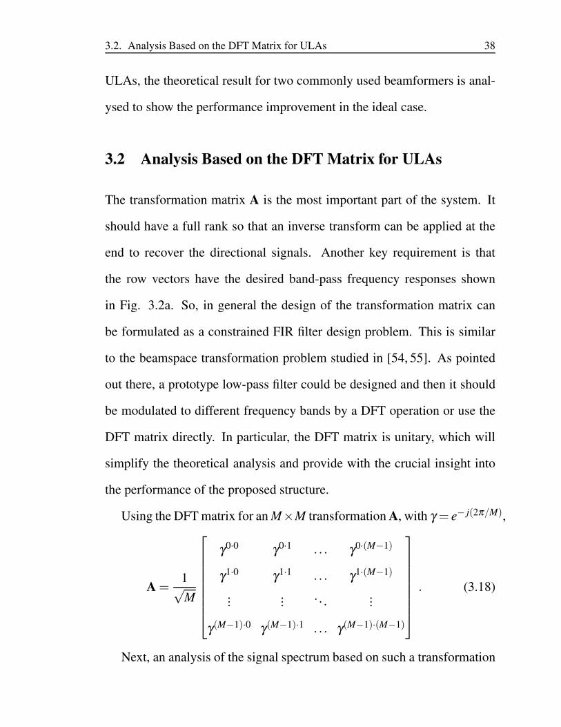
3.2 Analysis Based on the DFT Matrix for ULAs . . . . . . . . . . . . . . . 38
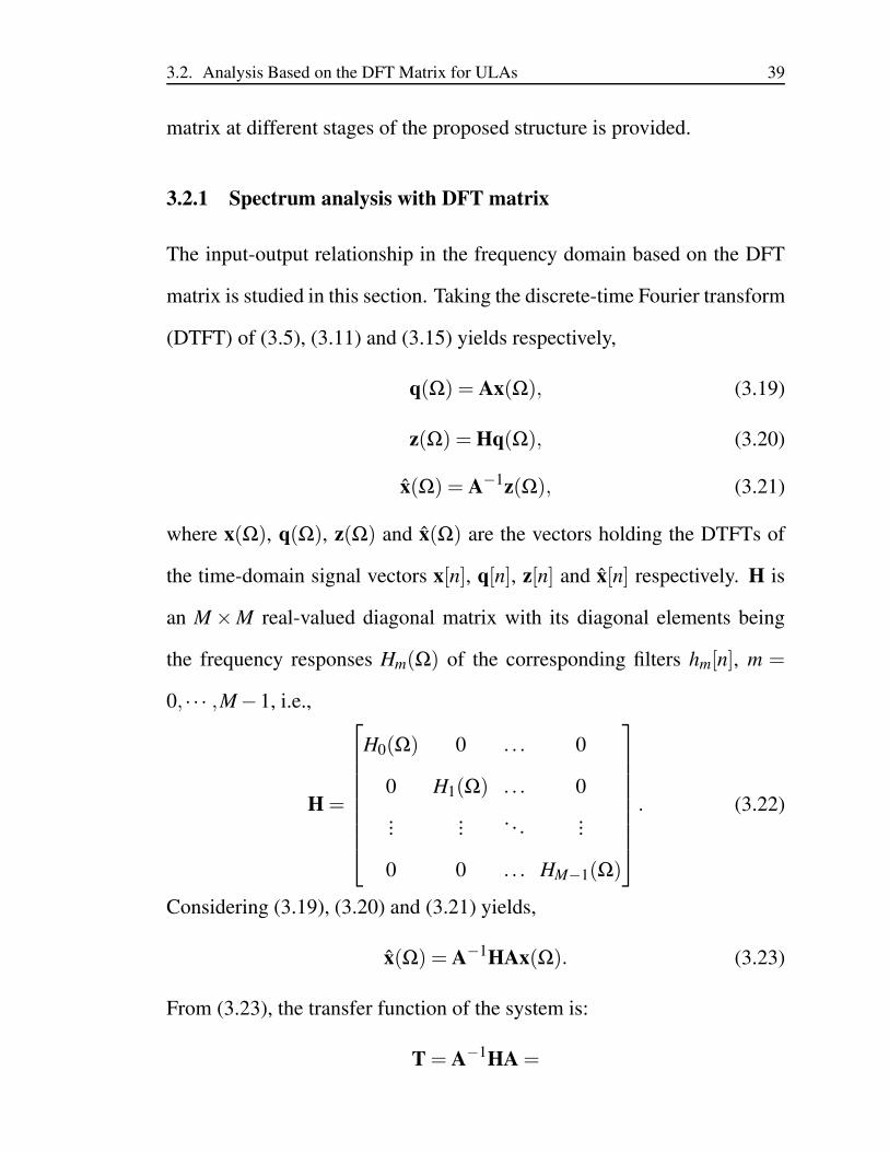
3.2.1 Spectrum analysis with DFT matrix . . . . . . . . . . . . . . . . 39
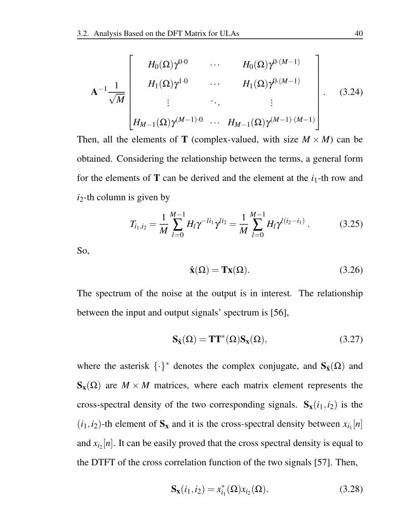
3.3 Performance Analysis of the Proposed Method . . . . . . . . . . . . . . 43
3.3.1 Reference signal based adaptive beamformer . . . . . . . . . . . 43
3.3.2 Linearly constrained minimum variance adaptive beamformer . . 45
3.4 Compressive Sensing Based DOA Estimation . . . . . . . . . . . . . . . 46
3.4.1 Introduction to compressive sensing . . . . . . . . . . . . . . . . 46
3.4.2 Signal model for DOA estimation . . . . . . . . . . . . . . . . . 48
3.4.3 Generating the virtual array . . . . . . . . . . . . . . . . . . . . 49
3.4.4 Narrowband DOA estimation . . . . . . . . . . . . . . . . . . . 50
3.4.5 Wideband DOA estimation . . . . . . . . . . . . . . . . . . . . . 50
3.5 Simulation Results . . . . . . . . . . . . . . . . . . . . . . . . . . . . . 54
3.5.1 The effect of the method on noise and directional signals . . . . . 56
3.5.2 The effect of the method on beamforming performance . . . . . . 60
3.5.3 The effect of the method on DOA estimation performance . . . . 64
3.6 Summary . . . . . . . . . . . . . . . . . . . . . . . . . . . . . . . . . . 66
4 Extension of the Noise Reduction Method for Non-uniform Linear Arrays 68
4.1 The Proposed White Noise Reduction for Non-uniform Linear Arrays . . 69
4.2 Least Squares Based Design for the Transformation Matrix . . . . . . . . 71
4.3 Simulation Results . . . . . . . . . . . . . . . . . . . . . . . . . . . . . 74
4.4 Fixing Ill Conditioned Transformation Matrix With SVD . . . . . . . . . 76
4.4.1 Simulation . . . . . . . . . . . . . . . . . . . . . . . . . . . . . 78
4.5 Summary . . . . . . . . . . . . . . . . . . . . . . . . . . . . . . . . . . 80
iv

5 Extension of the Method to Planar Arrays 83
5.1 White Noise Reduction for URAs with a 2D Transformation . . . . . . . 84
5.2 White Noise Reduction for URAs with a 1D Transformation . . . . . . . 92
5.3 White Noise Reduction for UCAs . . . . . . . . . . . . . . . . . . . . . 95
5.4 Simulation Results . . . . . . . . . . . . . . . . . . . . . . . . . . . . . 99
5.4.1 Simulation for the URA structure . . . . . . . . . . . . . . . . . 100
5.4.2 Simulation for the UCA structure . . . . . . . . . . . . . . . . . 106
5.5 Summary . . . . . . . . . . . . . . . . . . . . . . . . . . . . . . . . . . 107
6 Further Insights into the Proposed Noise Reduction Method 110
6.1 The TDL Equivalent Structure . . . . . . . . . . . . . . . . . . . . . . . 111
6.2 Computational Complexity of the Method . . . . . . . . . . . . . . . . . 113
6.3 Simulation Results . . . . . . . . . . . . . . . . . . . . . . . . . . . . . 113
6.4 Summary . . . . . . . . . . . . . . . . . . . . . . . . . . . . . . . . . . 118
7 Conclusions and Future Work 120
7.1 Conclusions . . . . . . . . . . . . . . . . . . . . . . . . . . . . . . . . . 120
7.2 Future Work . . . . . . . . . . . . . . . . . . . . . . . . . . . . . . . . . 124
Appendix 126
Bibliography 127
v

List of Abbreviations:
ANC Active Noise Control
CRB Cramer-Rao Bound
CS Compressive Sensing
CSSM Coherent Signal Subspace Method
DFT Discrete Fourier Transform
DTFT Discrete-Time Fourier Transform
DOA Direction of Arrival
ESPRIT Estimation of Signal Parameters via Rotational Invariance Techniques
FFT Fast Fourier Transform
FIR Finite Impulse Response
ISSM Incoherent Signal Subspace Method
LCMV Linearly Constrained Minimum Variance
MSE Mean Square Error
MUSIC MUltiple Signal Classification
NLA Non-uniform Linear Array
NP Non-deterministic Polynomial-time
NR Noise Reduction
PSD Power Spectral Density
RMSE Root Mean Square Error
RSB Reference Signal Based
SBL Sparse Bayesian Learning
SINR Signal-to-Interference plus Noise Ratio
SIR Signal-to-Interference Ratio
SNR Signal-to-Noise Ratio
SRACV Sparse Representation of Array Covariance Vector
vi

SVD Singular Value Decomposition
TDL Tapped Delay-Line
TOPS Test of Orthogonality of Projected Subspaces method
TSNR Total Signal-to-Noise Ratio
ULA Uniform Linear Array
UCA Uniform Circular Array
URA Uniform Rectangular Array
ZP Zero Phase
vii
List of Figures
1.1 A simple beamformer with its output y[n] given by a linear combination
of the received array signals x0[n], x1[n], · · · , xM−1[n] weighted with the
coefficients w0, w1, · · · , wM−1. . . . . . . . . . . . . . . . . . . . . . . . 5
2.1 A general wideband beamformer with M sensors and J taps. . . . . . . . 14
2.2 The RSB adaptive beamforming structure. . . . . . . . . . . . . . . . . . 15
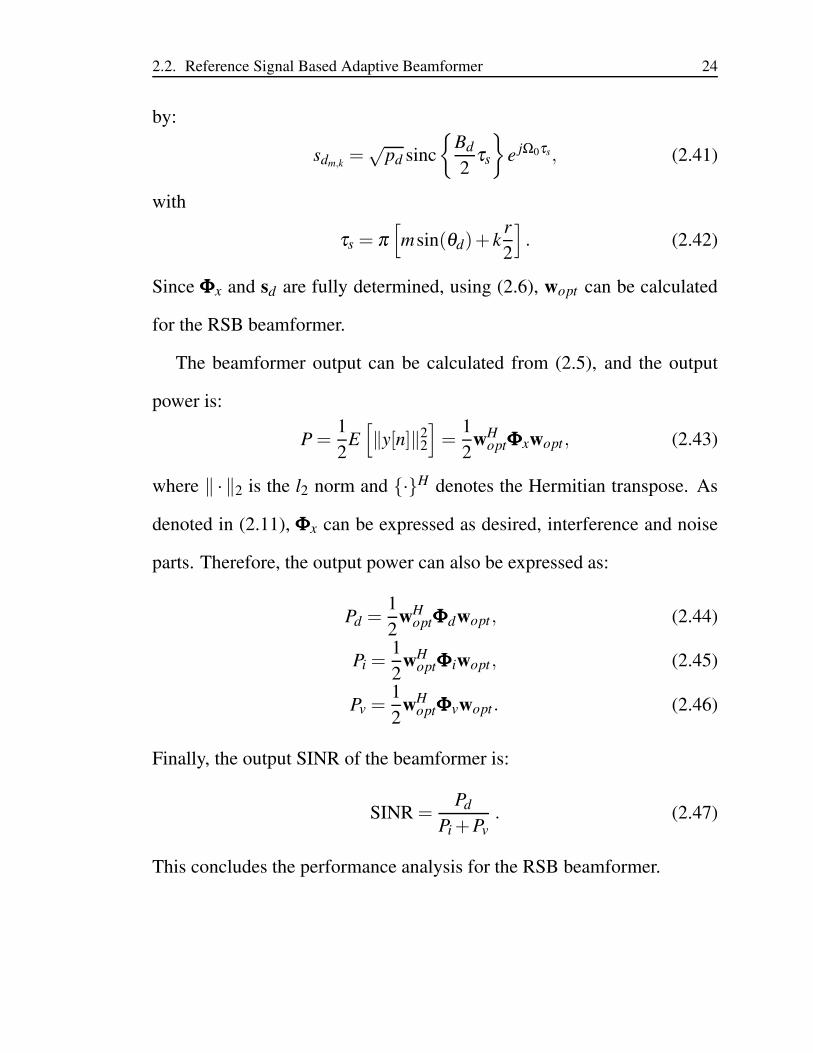
2.3 PSD of the desired signal. . . . . . . . . . . . . . . . . . . . . . . . . . . 18
2.4 The LCMV adaptive beamforming structure. . . . . . . . . . . . . . . . . 26
2.5 The equivalent single TDL beamformer for LCMV when the desired sig-
nal is arriving from broadside. . . . . . . . . . . . . . . . . . . . . . . . 26
3.1 A block diagram for the general structure of the proposed noise reduction
approach. . . . . . . . . . . . . . . . . . . . . . . . . . . . . . . . . . . 30
3.2 Frequency responses of the row vectors of A in the ideal case and the
high-pass filtering effect of a sample row vector. . . . . . . . . . . . . . . 33
3.3 Output to input noise power ratio for odd (M > 1) and even (M > 2) values
of M. . . . . . . . . . . . . . . . . . . . . . . . . . . . . . . . . . . . . 37
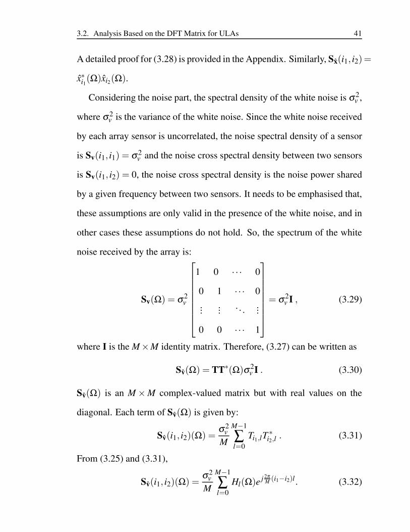
3.4 Power spectrum of the output of the noise reduction system with M=16. . 42
3.5 The frequency response of the 16×16 DFT matrix. . . . . . . . . . . . . 54
3.6 Frequency response of an example band-pass filter with M=16. . . . . . . 55
viii
3.7 Frequency response of the resultant beamformer with respect to normalised
signal frequency and DOA angle, when applying the filter coefficients in
Fig. 3.6 to the received array signal. . . . . . . . . . . . . . . . . . . . . 55
3.8 Frequency response of the 16 linear-phase 101-tap FIR high-pass filters. . 56
3.9 The beam pattern of a sample row vector before and after high-pass filter-
ing (ULA, M=16). . . . . . . . . . . . . . . . . . . . . . . . . . . . . . . 57
3.10 The power spectrum density of the spatially and temporally white noise
before and after processing (M=16). . . . . . . . . . . . . . . . . . . . . 58
3.11 SINR performance of both beamformers with and without the proposed
noise reduction (NR) method (M=16, J=100). . . . . . . . . . . . . . . . 62
3.12 SINR performance of both beamformers with and without the proposed
noise reduction method with regard to input SNR (M=16, J=100). . . . . 63
3.13 DOA estimation results with and without the proposed white noise reduc-
tion. . . . . . . . . . . . . . . . . . . . . . . . . . . . . . . . . . . . . . 65
3.14 RMSE vs input SNR. . . . . . . . . . . . . . . . . . . . . . . . . . . . . 66
4.1 Frequency response of the row vectors of the 15×15 designed transfor-
mation matrix for NLAs. . . . . . . . . . . . . . . . . . . . . . . . . . . 75
4.2 SINR performance of both beamformers with and without the proposed
noise reduction method for the NLA. . . . . . . . . . . . . . . . . . . . . 77
4.3 SINR performance of both beamformers with and without the modified
noise reduction (NR) methods for the NLA. . . . . . . . . . . . . . . . . 81
5.1 The structure of a URA, where a signal impinges from azimuth angle θ
and elevation angle φ . . . . . . . . . . . . . . . . . . . . . . . . . . . . 85
5.2 A block diagram of the proposed noise reduction method based on a 2D
transformation. . . . . . . . . . . . . . . . . . . . . . . . . . . . . . . . 86
5.3 Frequency responses of the 2D transformation applied to an M×N URA. 89
5.4 The high-pass filtering effect of the (m, l)-th 2D filter in the ideal case. . . 90
ix
5.5 The high-pass filtering effect of the (m, l)-th 2D filter in the signal fre-
quency domain in the ideal case. . . . . . . . . . . . . . . . . . . . . . . 90
5.6 The general structure for UCA. . . . . . . . . . . . . . . . . . . . . . . . 96
5.7 Frequency responses of an example 2D-DFT vector and its corresponding
1D-DFT vector, for the directional signal arriving from θ = 90 and φ = 45.101
5.8 SINR performance of both beamformers with and without the proposed
noise reduction (NR) methods for the URA. . . . . . . . . . . . . . . . . 104
5.9 SINR performance of the RSB beamformer with the desired signal arriv-
ing from θd = 5 and φd = 0. . . . . . . . . . . . . . . . . . . . . . . . 105
5.10 The beam-pattern of a sample row vector of the transformation designed
for UCA, before and after modifying the condition number, M = 30, φ =
90. . . . . . . . . . . . . . . . . . . . . . . . . . . . . . . . . . . . . . 107
5.11 SINR performance of both beamformers with and without the modified
noise reduction (NR) methods for the UCA, M = 30, J = 5. . . . . . . . . 108
6.1 SINR performance of RSB beamformer with NR method and without NR
with equivalent length, lhp = 101. . . . . . . . . . . . . . . . . . . . . . 115
6.2 SINR performance of LCMV beamformer with NR method and without
NR with equivalent length, lhp = 101. . . . . . . . . . . . . . . . . . . . 116
6.3 SINR performance of both beamformers with respect to number of taps,
with NR method and without NR with equivalent length Jeq. . . . . . . . 117
x
List of Tables
3.1 MSE for the directional signal. . . . . . . . . . . . . . . . . . . . . . . . 60
3.2 Power loss for the white noise. . . . . . . . . . . . . . . . . . . . . . . . 60
4.1 Sensor locations for the wideband NLA example. . . . . . . . . . . . . . 74
5.1 MSE for the directional signal before and after the proposed noise reduc-
tion process for different URA sizes. . . . . . . . . . . . . . . . . . . . . 102
6.1 Computational complexity of the noise reduction based implementation,
the RSB and LCMV beamformers. . . . . . . . . . . . . . . . . . . . . . 113
6.2 Computation time of the noise reduction based implementation, the RSB
and LCMV beamformers. . . . . . . . . . . . . . . . . . . . . . . . . . . 118
xi
List of Publications:
Journal papers:
1. M. R. Anbiyaei, W. Liu, and D. C. McLernon, “ White noise reduc-
tion for wideband linear array signal processing”, IET Signal Pro-
cessing, DOI: 10.1049/iet-spr.2016.0730, accepted, yet to appear in
the printed journal.
Conference papers:
1. M. R. Anbiyaei, W. Liu, and D. C. McLernon, “Performance im-
provement for wideband beamforming with white noise reduction
based on sparse arrays”, in Proc. 25th European Signal Processing
Conference, pp. 2433-2437, Greece, September 2017.
2. M. R. Anbiyaei, W. Liu, and D. C. McLernon, “White noise reduction
for wideband beamforming based on uniform rectangular arrays”, in
Proc. 22nd Digital Signal Processing Conference, pp. 1-5, London,
UK, August 2017.
3. M. R. Anbiyaei, W. Liu, and D. C. McLernon, “Performance im-
provement for wideband DOA estimation with white noise reduction
based on uniform linear arrays,” in Proc. IEEE, 9th Sensor Array and
Multichannel Signal Processing Workshop (SAM), pp. 1-5, Rio de
Janeiro, Brazil, July 2016.
xii

Acknowledgements:
I would like to take this opportunity to express my deepest gratitude to
my supervisor Dr. Wei Liu for his persistent encouragement, guidance and
support, and also for giving me the opportunity to pursue my PhD studies
under his supervision.
I also thank my second supervisor Dr. Xiaoli Chu for her help and
support regarding the doctoral development program.
Finally, I would like to thank my parents for their continuous encour-
agement and support.
xiii
Chapter 1
Introduction
1.1 Introduction
Wideband array signal processing, including beamforming and direction
of arrival (DOA) estimation, has various applications in radar, sonar and
wireless communications, and has been studied extensively in the past.
In [1], different adaptive beamformer methods and parameter estima-
tion is reviewed thoroughly. Wei et. al [2] has reviewed different methods
of beamforming and array structures. Krim and Vberg review background
material and of the basic problem formulation of the parameter estimation
in [3]. They introduce spectral-based algorithmic solutions to the signal
parameter estimation problem, and the suboptimal solutions are compared
to the parametric methods. Allen and Ghavami review the fundamentals
of array signal processing in [4], and they review different adaptive beam-
forming and estimation methods considering both narrowband and wide-
band cases. Some difficulties and practical techniques related to sensor
1
1.1. Introduction 2
arrays are addressed in [5]. Such as, placing sensors as an array for accu-
rate measurement, calibrating a sensor array by experiment and etc.
The performance of wideband array signal processing algorithms is de-
pendent on the level of noise in the system, and normally the lower the
level of noise, the better the performance is. Many methods have been
developed in the past to reduce the noise level, such as adaptive noise can-
cellation (ANC) [6], the Wiener filters [7,8], and zero phase (ZP) noise re-
duction methods [9,10]. The ANC uses a reference undesired noise source
and a primary source contaminated by noise, and then adaptive filtering is
employed to produce a cleaned result [11]. The Wiener filter produces an
estimate of the desired signal by minimising the mean squared error (MSE)
between the noisy signal and a reference [12, 13]. The ANC and Wiener
filter methods have proved to work well in specific applications but due to
their adaptive nature, they have high computational complexity. ZP noise
reducers can reduce the noise without the need to know a priori information
of the signal [14,15]. The limitation of ZP noise reducers is that, the signal
has to be periodic [16], and it is mainly applied to speech signals. In this
thesis, a novel non-adaptive white noise reduction approach is developed
with low computational complexity, and relatively good performance, with
no limitation on the received wideband signal.
In addition to the wideband beamforming, the wideband DOA estima-
tion is also a field of interest in this thesis. Many DOA methods have
been proposed for both narrowband and wideband signals, and two rep-
1.1. Introduction 3
resentative ones are the multiple signal classification (MUSIC) [17] and
the estimation of signal parameters via rotational invariance techniques
(ESPRIT) [18] algorithms, which were originally proposed for narrow-
band signals. For wideband signals, a commonly used approach is to
decompose the wideband signal into different frequency bins and trans-
form the wideband problem into a narrowband one through various fo-
cusing or interpolation algorithms [19, 20]. In addition, methods such
as incoherent signal subspace method (ISSM) [21], coherent signal sub-
space method (CSSM) [22] and test of orthogonality of projected sub-
spaces method (TOPS) [23] have also been proposed.
Recently, with the development of compressive sensing theory [24,25],
many sparsity based DOA estimation methods were developed. A source
localization method based on a sparse representation of sensor measure-
ments is introduced in [26]. In [27], a DOA estimation method is proposed
based on a novel data model using the concept of a sparse representation of
array covariance vectors (SRACV), in which DOA estimation is achieved
by jointly finding the sparsest coefficients of the array covariance vectors.
The sparse spectrum fitting algorithm for the estimation of DOAs of mul-
tiple sources is introduced in [28], and its asymptotic consistency and ef-
fective regularization under both asymptotic and finite sample cases are
studied. In [29], the authors propose co-prime arrays for effective DOA
estimation.
In addition, various extensions of the above methods are developed for
1.1. Introduction 4
the wideband case. A method named wideband covariance matrix sparse
representation (W-CMSR) is proposed in [30]. In this method, the lower
left triangular elements of the covariance matrix are aligned to form a
new measurement vector, then DOA estimation is achieved by representing
this vector on an over-complete dictionary under the constraint of sparsity.
In [31], the sparse Bayesian learning (SBL) technique is used to estimate
the DOAs of independent narrowband/wideband signals by reconstructing
the covariance vectors with high computational efficiency. In [32], a class
of low-complexity compressive sensing-based DOA estimation methods
for wideband co-prime arrays is proposed, which is based on the narrow-
band DOA estimation method for co-prime arrays [29].
Wideband arrays are affected by noise from different sources. These
noise sources include the voltages due to thermal noise [33] also known
as Johnson-Nyquist noise [34], the shot noise [35], the cosmic black-body
radiation [36] and etc. The classical central limit theorem [37] asserts that
the distribution of the summation of different random variables converges
to a normal, Gaussian distribution with mean 0, which is the definition of
the white noise. Therefore, one common assumption for noise in wideband
arrays is that it is spatially (and in many cases also temporally) white. That
is, the noise at one array sensor is uncorrelated with that at other sensors.
Under this assumption, it seems that there is not much can be done about
it and simply it has to be accepted whatever is left of the noise component
after processing the signals. For example, in the simplest beamforming
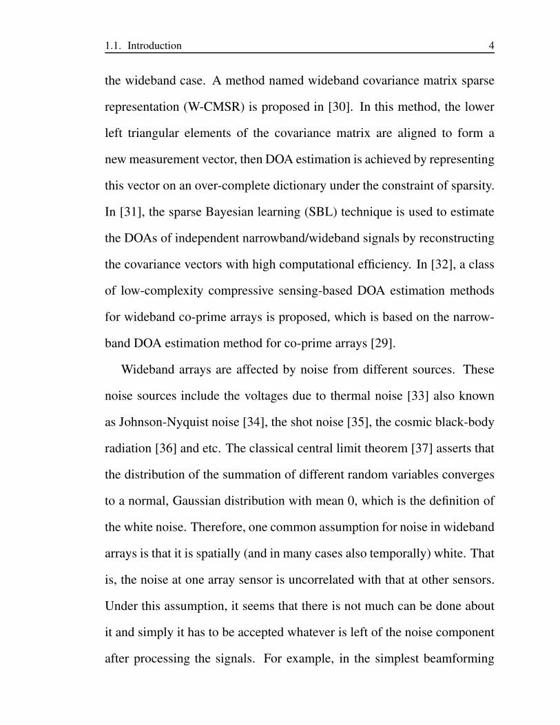
1.1. Introduction 5
y[n]
x0[n]
w1
w0
θ x1[n]
xM−1[n] wM−1
Fig. 1.1: A simple beamformer with its output y[n] given by a linear combination of the
received array signals x0[n], x1[n], · · · , xM−1[n] weighted with the coefficients w0, w1, · · · ,
wM−1.
structure shown in Fig. 1.1, the beamformer output y[n] is a linear combi-
nation of the received array signals x0[n], x1[n], · · · , xM−1[n] weighted with
the coefficients w0, w1, · · · , wM−1, where n is the discrete time index, M
is the number of sensors in the array and θ is the angle of arrival of the
impinging signal. The values of these coefficients are obtained based on
some criterion such as maximising the output signal-to-interference plus
noise ratio (SINR).
The question here is, whether there is anything that can be done to re-
duce the effect of the white noise in a wideband array system (without at-
tenuating the directional signals) so that the performance of the subsequent
processing (such as DOA estimation and beamforming) can be improved.
In this thesis, the aim is to answer that question by developing a novel
method to reduce the white noise level of a wideband array using a combi-
1.1. Introduction 6
nation of a set of judiciously designed spatial transformations and a bank of
high-pass filters, and the key is to realise that the white noise and the direc-
tional wideband signals received by the array have different spatial char-
acteristics. Based on this difference, and motivated by the low-complexity
subband-selective adaptive beamformer proposed in [38], first the received
wideband sensor signals is transformed into a new domain where the di-
rectional signals are decomposed in such a way that their corresponding
outputs are associated with a series of tighter and tighter high-pass spec-
tra, while the spectrum of noise still covers the full band from −π to π in
the normalised frequency domain. Then, a series of high-pass filters with
different cut-off frequencies are applied to selectively remove part of the
noise spectrum while keeping the directional signals unchanged. Finally,
an inverse transformation is applied to the filtered outputs to recover the
original sensor signals, where compared to the original set of received sen-
sor signals, the directional signals are left intact while the noise power has
been reduced.
One condition placed on the transformation matrix is that it must be
invertible. It has been further assumed that it is also unitary and thus the
discrete Fourier transform (DFT) matrix is used as a representative exam-
ple for the uniform linear array (ULA) case and a least squares based de-
sign is introduced for the non-uniform linear array (NLA) case. Detailed
analysis shows that the signal-to-noise ratio (SNR) of the array after the
proposed processing can be improved by about 3 dB in the ideal case. This
1.2. Original Contributions 7
is then translated into improved performance for beamforming, as demon-
strated by both theoretical analysis and simulation results. This work is fo-
cused on two well-known beamformers, namely the reference signal based
(RSB) [39, 40], and the linearly constrained minimum variance (LCMV)
beamformers [41].
The method is also extended to uniform rectangular arrays (URAs), and
uniform circular arrays (UCAs) as examples of planar arrays.
1.2 Original Contributions
The original contributions of this work to the field of array signal process-
ing are listed as follows,
• The SNR of the received signal can be improved by a maximum of
3 dB using the proposed noise reduction method for different array
structures such as ULA, NLA, URA and UCA which have been pre-
sented in this work.
• Using the developed noise reduction method an increased output SINR
performance is achieved for the classic RSB and LCMV beamform-
ers, for different array structures.
• Simulation results show an improved estimation accuracy for the com-
pressive sensing based DOA estimation for the ULA structure.
• The method provides an alternative approach to beamforming with
1.2. Original Contributions 8
reduced computational complexity and more robustness.
• No prior information of the impinging signal is needed and the method
is quite flexible. Therefore, it can be used for different array signal
processing applications, such as beamforming and DOA estimation.
In the following, the contributions of the work are explained in greater
detail.
1.2.1 White noise reduction for wideband uniform linear array sig-
nal processing with applications in beamforming and DOA es-
timation
A novel method is proposed for reducing the level of white noise in wide-
band ULAs via a judiciously designed spatial transformation followed by
a bank of high-pass filters. 3 dB improvement in total SNR is achieved by
this method. A detailed analysis of the method and its effect on the spec-
trum of the signal and noise is presented. The reduced noise level leads
to a higher SNR for the system, which can have significant effect on the
performance of various beamforming methods and other signal processing
applications, such as DOA estimation.
The improved performance of two well-known beamformers, namely,
the RSB and the LCMV beamformers is analysed. Initially, a detailed
theoretical performance analysis is presented, and then, the improved per-
formance is confirmed using simulation.
1.2. Original Contributions 9
A compressive sensing based method employing the group sparsity con-
cept is employed to analyse the performance improvement for DOA esti-
mation. The performance is evaluated by calculating the error between the
estimated and the actual DOA angles of the received signals. By apply-
ing the noise reduction method, the error between the estimated and the
actual DOA angles was reduced. Therefore, the estimation accuracy has
been improved by employing the noise reduction method. The improved
estimation accuracy is confirmed by simulation.
By studying the structure of the method further, it is understood that if
a classic beamformer is applied to a set of array signals which have been
processed by the noise reduction method, the pre-processing and the clas-
sic beamformer can be modelled as an equivalent beamformer with longer
TDLs. Additionally, the complexity of the noise reduction method includ-
ing the beamformer part is less than the direct implementation with equiv-
alent length. Also, with the noise reduction method, a more robust beam-
forming can be achieved, since by using the noise reduction pre-processing
the numerical issues due to calculating the optimum beamforming coeffi-
cients based on inversion of correlation matrices can be avoided.
1.2.2 Extension of the white noise reduction method for non-uniform
linear arrays
The idea is extended to the NLAs by redesigning the transformation using
least squares filter design method. Therefore, the noise reduction method
1.2. Original Contributions 10
is adjusted to be applicable to the non-uniform sensor layout of NLAs. A
prototype filter using least squares method is designed, and modulated to
different frequency subbands to cover the whole normalised spectrum. A
low condition number is crucial, to be certain that the transformation is
invertible. Initially, the diagonal loading method is used to keep the con-
dition number low. Similar to the ULA case, 3 dB improvement in total
SNR is achieved, which leads to the performance enhancement for beam-
forming. This enhancement is demonstrated by simulation, using RSB and
LCMV beamformers.
Also, for reducing the condition number of the designed transforma-
tion matrix, a modification method is proposed based on replacing the
small singular values of the transformation. The effect of this modification
method on the beam-pattern and the condition number of the transforma-
tion is presented, and the beamforming performance of the noise reduction
method using the modified transformation is investigated using simulation.
1.2.3 Extension of the white noise reduction method for planar ar-
rays
The idea is also extended to two major types of planar arrays, namely,
URAs and UCAs.
In case of the URA, two design methods are introduced for the noise
reduction method, and for each one the transformation is redesigned. The
first method is based on a two-dimensional (2D) transformation, and the
1.3. Outline 11
second one is an adaptation of the ULA noise reduction method, which is
based on one-dimensional (1D) transformation of the received signals.
For the UCA case, a 1D transformation is presented, which is almost
similar to the ULA case, and the difference is in modulating the prototype
filter to different subbands. Due to the sparse nature of circular arrays,
the condition number of the transformation might be high, which is in this
case, and the condition number is reduced by replacing the small singular
values of the transformation, same as in the NLA case.
The effect of the noise reduction methods for the planar arrays on per-
formance improvement of RSB and LCMV beamformers is confirmed by
simulation.
1.3 Outline
This thesis is organised as follows.
In Chapter 2, the wideband beamforming is briefly reviewed and a de-
tailed theoretical performance analysis is provided for the two well-known
classic beamformers, namely, RSB and LCMV beamformers. These two
beamformers are used for different applications in this thesis.
The white noise reduction method based on the ULA structure is pro-
posed in Chapter 3, with a detailed analysis of the spectrum and correla-
tion matrix of the noise after the proposed processing, when DFT matrix is
used as transformation. Then, the effect of the noise reduction method on
1.3. Outline 12
the performance enhancement of the RSB and LCMV beamformers and
a compressive sensing based DOA estimation is presented, and confirmed
by simulation results.
The idea is extended to the structure of the NLAs in Chapter 4. The least
squares approach is used for designing the transformation with satisfactory
band-pass response.
The idea is further extended to the URA and UCA structures as exam-
ples of the planar arrays in Chapter 5, where two methods are presented
for the URA case, one based on 2D filtering and one by directly adopting
the method developed for the ULA structure. For the UCA case, the mod-
ulation of the row vectors of the transformation is modified to satisfy the
structure of the UCA.
In Chapter 6, it is shown that the proposed noise reduction method is
equivalent to a traditional tapped delay-line (TDL) system. The perfor-
mance and computational complexity of the beamformers are compared,
with the proposed pre-processing and without any pre-processing with the
same length.
Finally, conclusions are drawn in Chapter 7, with possible topics for
future work.
Chapter 2
Adaptive Wideband Beamforming
In this chapter, the general idea of wideband beamforming is briefly re-
viewed. The RSB and LCMV beamformers are reviewed as examples for
adaptive wideband beamforming, and a detailed analysis of their perfor-
mance is provided.
2.1 Wideband Beamforming
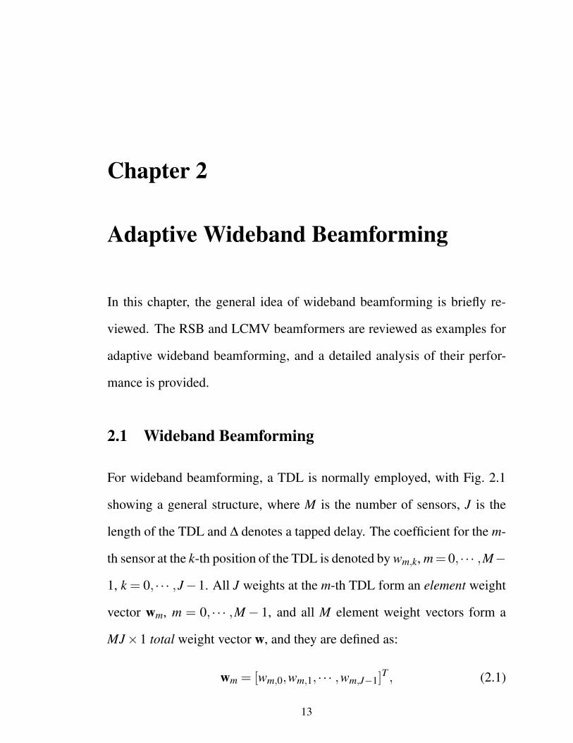
For wideband beamforming, a TDL is normally employed, with Fig. 2.1
showing a general structure, where M is the number of sensors, J is the
length of the TDL and ∆ denotes a tapped delay. The coefficient for the m-
th sensor at the k-th position of the TDL is denoted by wm,k, m= 0, · · · ,M−
1, k = 0, · · · ,J−1. All J weights at the m-th TDL form an element weight
vector wm, m = 0, · · · ,M − 1, and all M element weight vectors form a
MJ×1 total weight vector w, and they are defined as:
wm = [wm,0,wm,1, · · · ,wm,J−1]T , (2.1)
13
2.1. Wideband Beamforming 14
,
,,0
,0
,1
,1
n
M−1 M−1M−1
w0 w0 −1J
M−1 ][nx
][x0
w w w −1J
][y n
w0
Fig. 2.1: A general wideband beamformer with M sensors and J taps.
w =[
wT0 ,w
T1 , · · ·wT
M−1
]T, (2.2)
where ·T denotes the transpose. The received signal by the m-th sensor
at the k-th position of the TDL is denoted by xm,k[n], m = 0, · · · ,M − 1,
k = 0, · · · ,J − 1. All J received signals at the m-th TDL form an element
signal vector xm, m = 0, · · · ,M−1 and all M element signal vectors form
the total input signal vector x, which are defined as:
xm =[
xm,0[n],xm,1[n], · · · ,xm,M−1[n]]T
, (2.3)
x = [xT0 ,x
T1 , · · · ,xT
M−1]T . (2.4)
Finally, the beamformer output y[n] is given by
y[n] = wT x . (2.5)
The idea is to process the received array signals by the noise reduc-
tion method, so that the noise level in the received signals will be reduced.
Then, the new set of array signals with reduced noise level will be fed to the
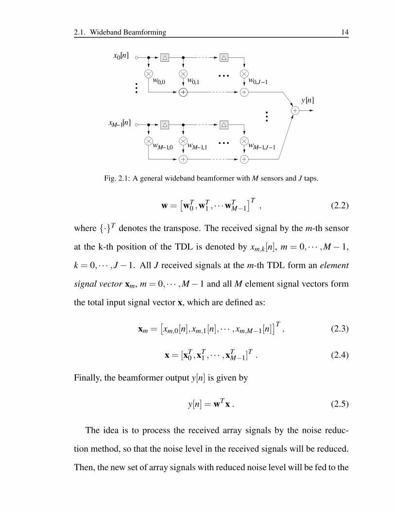
2.2. Reference Signal Based Adaptive Beamformer 15
+-
+r[n]e[n]
x[n] y[n]w
Fig. 2.2: The RSB adaptive beamforming structure.
following beamformers. In the following, two widely-used adaptive beam-
forming methods are briefly reviewed and the theoretical performance re-
sults are then derived based on the proposed noise reduction method.
2.2 Reference Signal Based Adaptive Beamformer
The reference signal based (RSB) beamformer is normally employed when
a reference signal r[n] is available, where the weight vector of the beam-
former can be adjusted to minimise the MSE between the reference signal
and the beamformer output y[n] [39,40], as shown in Fig. 2.2. The MJ×1
optimal weight vector is given by:
wopt =ΦΦΦx−1sd , (2.6)
where ·−1 denotes the inverse operator, ΦΦΦx is the signal correlation ma-
trix with size MJ×MJ, and is defined by:
ΦΦΦx = E[
x∗xT]
, (2.7)
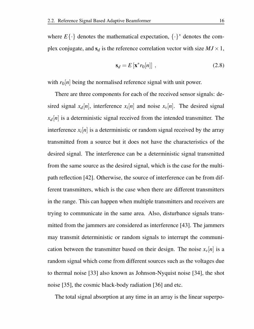
2.2. Reference Signal Based Adaptive Beamformer 16
where E· denotes the mathematical expectation, ·∗ denotes the com-
plex conjugate, and sd is the reference correlation vector with size MJ×1,
sd = E [x∗r0[n]] , (2.8)
with r0[n] being the normalised reference signal with unit power.
There are three components for each of the received sensor signals: de-
sired signal xd[n], interference xi[n] and noise xv[n]. The desired signal
xd[n] is a deterministic signal received from the intended transmitter. The
interference xi[n] is a deterministic or random signal received by the array
transmitted from a source but it does not have the characteristics of the
desired signal. The interference can be a deterministic signal transmitted
from the same source as the desired signal, which is the case for the multi-
path reflection [42]. Otherwise, the source of interference can be from dif-
ferent transmitters, which is the case when there are different transmitters
in the range. This can happen when multiple transmitters and receivers are
trying to communicate in the same area. Also, disturbance signals trans-
mitted from the jammers are considered as interference [43]. The jammers
may transmit deterministic or random signals to interrupt the communi-
cation between the transmitter based on their design. The noise xv[n] is a
random signal which come from different sources such as the voltages due
to thermal noise [33] also known as Johnson-Nyquist noise [34], the shot
noise [35], the cosmic black-body radiation [36] and etc.
The total signal absorption at any time in an array is the linear superpo-
2.2. Reference Signal Based Adaptive Beamformer 17
sition of the absorption associated with all the impinging signals and the
noise [44, 45]. Therefore, the signal available at the m-th sensor and k-th
tap is,
xm,k[n] = xdm,k[n]+ xim,k[n]+ xvm,k[n] . (2.9)
So, the total signal vector x can also be decomposed into three correspond-
ing parts:
x = xd +xi +xv. (2.10)
Since the desired signal, interference and noise are independent and so,
uncorrelated with each other, ΦΦΦx is also a linear superposition of the cor-
responding parts and can be decomposed into three MJ ×MJ correlation
matrices corresponding to the desired signal, interference and white noise
components, respectively. i.e.,
ΦΦΦx =ΦΦΦd +ΦΦΦi +ΦΦΦv . (2.11)
In the following, each of the correlation matrices from (2.11) are deter-
mined.
First, the desired signal part is considered. To simplify the theoretical
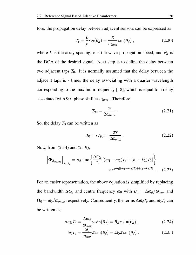
calculations, it is assumed that the desired signal xd[n] has a flat power
spectral density (PSD) equal to 2π pd/∆ωd , where pd, ωd and ∆ωd are the
power, frequency, and bandwidth of the desired signal, respectively. The
PSD of the desired signal Sd(ω) is illustrated in Fig. (2.3) with ω0 being
the centre frequency.
The auto-correlation is a measure of the correlation between the values
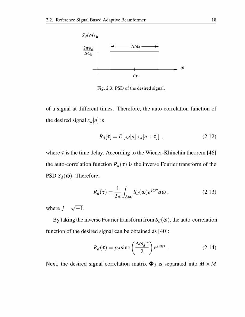
2.2. Reference Signal Based Adaptive Beamformer 18
ω
∆ωd2π pd∆ωd
ω0
Sd(ω)
Fig. 2.3: PSD of the desired signal.
of a signal at different times. Therefore, the auto-correlation function of
the desired signal xd[n] is
Rd[τ] = E [xd[n] xd[n+ τ]] , (2.12)
where τ is the time delay. According to the Wiener-Khinchin theorem [46]
the auto-correlation function Rd(τ) is the inverse Fourier transform of the
PSD Sd(ω). Therefore,
Rd(τ) =1
2π
∫
∆ωd
Sd(ω)e jωτdω , (2.13)
where j =√−1.
By taking the inverse Fourier transform from Sd(ω), the auto-correlation
function of the desired signal can be obtained as [40]:
Rd(τ) = pd sinc
(
∆ωdτ
2
)
e jω0τ . (2.14)
Next, the desired signal correlation matrix ΦΦΦd is separated into M ×M
2.2. Reference Signal Based Adaptive Beamformer 19
sub-matrices as:
ΦΦΦd =
ΦΦΦd0,0· · · ΦΦΦd0,M−1
.... . .
...
ΦΦΦdM−1,0· · · ΦΦΦdM−1,M−1
, (2.15)
where each correlation sub-matrix is a J× J matrix and corresponds to the
correlation of the desired signal of two different element signal vectors.
Therefore,
ΦΦΦdm1,m2= E
[
x∗dm1xT
dm2
]
. (2.16)
Note that the correlation between the desired signal at the k1-th tap of the
m1-th element and the k2-th tap of m2-th element is given by:
[
ΦΦΦdm1,m2
]
k1,k2
= E[
x∗dm1,k1[n] xdm2,k2
[n]]
. (2.17)
The desired signal received at the m-th element and the k-th tap is a copy of
the original desired signal with a delay among the array elements, as well
a delay among taps. So
xdm,k[n] = xd [n−mTe− kT0] , (2.18)
where Te is the unit propagation delay between elements, and T0 is the
propagation delay between adjacent taps. So, (2.17) can be written as:
[
ΦΦΦdm1,m2
]
k1,k2
= Rd [(m1 −m2)Te +(k1− k2)T0] . (2.19)
It is assumed that the adjacent array sensor spacing is half a wavelength
of the maximum frequency ωmax to avoid the spatial aliasing [47]. There-
2.2. Reference Signal Based Adaptive Beamformer 20
fore, the propagation delay between adjacent sensors can be expressed as
Te =L
csin(θd) =
π
ωmaxsin(θd) , (2.20)
where L is the array spacing, c is the wave propagation speed, and θd is
the DOA of the desired signal. Next step is to define the delay between
two adjacent taps T0. It is normally assumed that the delay between the
adjacent taps is r times the delay associating with a quarter wavelength
corresponding to the maximum frequency [48], which is equal to a delay
associated with 90 phase shift at ωmax . Therefore,
T90 =π
2ωmax. (2.21)
So, the delay T0 can be written as
T0 = rT90 =πr
2ωmax. (2.22)
Now, from (2.14) and (2.19),
[
ΦΦΦdm1,m2
]
k1,k2
= pd sinc
∆ωd
2[(m1−m2)Te +(k1− k2)T0]
×e jω0[(m1−m2)Te+(k1−k2)T0] . (2.23)
For an easier representation, the above equation is simplified by replacing
the bandwidth ∆ωd and centre frequency ω0 with Bd = ∆ωd/ωmax and
Ω0 = ω0/ωmax, respectively. Consequently, the terms ∆ωdTe and ω0Te can
be written as,
∆ωdTe =∆ωd
ωmaxπ sin(θd) = Bdπ sin(θd) , (2.24)
ω0Te =ω0
ωmaxπ sin(θd) = Ω0π sin(θd) . (2.25)
2.2. Reference Signal Based Adaptive Beamformer 21
Similarly, ∆ωdT0 and ω0T0 are written as,
∆ωdT0 =∆ωd
ωmax· πr
2= Bd
πr
2, (2.26)
ω0T0 =ω0
ωmax· πr
2= Ω0
πr
2. (2.27)
Therefore, in the simplified form, the correlation of the desired signal at
the k1-th tap of the m1-th element and the k2-th tap of the m2-th element
can be expressed as,
[
ΦΦΦdm1,m2
]
k1,k2
= pd sinc
Bd
2τd
e jΩ0τd , (2.28)
where τd is,
τd = π[
(m1 −m2)sin(θd)+(k1− k2)r
2
]
. (2.29)
Next step is to determine the interference correlation matrix ΦΦΦi using
the same approach. The DOA θi of the interference is different from θd .
Same as before, to simplify the theoretical calculations, it is been assumed
that the interference signal xi[n] has a flat PSD, equal to 2π pi/∆ωi, where
pi, ωi and ∆ωi are the power, frequency and bandwidth of the interference
signal, respectively. Same as (2.15), the interference correlation matrix ΦΦΦi
is separated into M×M sub-matrices as:
ΦΦΦi =
ΦΦΦi0,0 · · · ΦΦΦi0,M−1
.... . .
...
ΦΦΦiM−1,0 · · · ΦΦΦiM−1,M−1
, (2.30)
where each correlation sub-matrix is a J × J matrix, corresponding to the
correlation of the interference of two different element interference signal
2.2. Reference Signal Based Adaptive Beamformer 22
vectors,
ΦΦΦim1,m2= E
[
x∗im1xT
im2
]
. (2.31)
The correlation between the interference at the k1-th tap of the m1-th ele-
ment and the k2-th tap of the m2-th element is:
[
ΦΦΦim1,m2
]
k1,k2
= E[
x∗im1,k1[n] xim2,k2
[n]]
. (2.32)
Similar to the desired signal in (2.28), in the simplified form, the correla-
tion of the interference at the k1-th tap of the m1-th element and the k2-th
tap of the m2-th element can be expressed as:
[
ΦΦΦim1,m2
]
k1,k2
= pi sinc
Bi
2τi
e jΩ0τi , (2.33)
where Bi = ∆ωi/ω0 and τi is
τi = π[
(m1 −m2)sin(θi)+(k1 − k2)r
2
]
. (2.34)
Since it is assumed that the noise available at each sensor is temporally
and also spatially white, so the noise is mathematically independent be-
tween the sensors in the TDL. Therefore, the noise correlation products of
the correlation matrix in (2.11) are zero, apart from the product of the same
delay-line. Similar to (2.15) and (2.30), the noise correlation matrix ΦΦΦv is
also separated into M×M sub-matrices, so:
ΦΦΦv =
ΦΦΦv0,0 0 · · · 0
0 ΦΦΦv1,1 · · · 0
......
. . ....
0 0 · · · ΦΦΦvM−1,M−1
, (2.35)
2.2. Reference Signal Based Adaptive Beamformer 23
where each non-zero noise correlation sub-matrix is a J × J matrix. It is
assumed the white noise has a flat PSD equal to 2πσ2v /∆ωv, where σ2
v is
the noise variance and ∆ωv is the bandwidth of the noise. Therefore, as in
(2.28) and (2.33), the correlation of the noise at the k1-th and k2-th tap of
the same m1-th element is
[ΦΦΦvm1,m1]k1,k2
= σ2v sinc
Bv
2τv
e jΩ0τv, (2.36)
where Bv = ∆ωv/ω0 and τv is
τv = π[
(k1− k2)r
2
]
. (2.37)
Finally, the reference correlation vector sd is determined. Assuming the
reference signal ro[n] is the same as the desired signal xd[n], sd in (2.8) can
be written as
sd = E[x∗ro[n]] = E[x∗xdo[n]] . (2.38)
where xdo[n] is the same as xd[n], with unit power. It has been assumed that
the desired signal, interferences and the noise are uncorrelated with each
other. Therefore, (2.38) can be expressed as:
sd = E[x∗dxdo[n]] . (2.39)
Furthermore, sd can be expanded as:
sd =[
sd0,0, · · · ,sd0,J−1
, · · · ,sdM−1,0, · · · ,sdM−1,J−1
]T, (2.40)
where sdm,k, m = 0, · · · ,M−1, k = 0, · · · ,J−1, indicates the correlation of
the reference and the desired signal at the m-th element and k-th tap, given
2.2. Reference Signal Based Adaptive Beamformer 24
by:
sdm,k=√
pd sinc
Bd
2τs
e jΩ0τs, (2.41)
with
τs = π[
msin(θd)+ kr
2
]
. (2.42)
Since ΦΦΦx and sd are fully determined, using (2.6), wopt can be calculated
for the RSB beamformer.
The beamformer output can be calculated from (2.5), and the output
power is:
P =1
2E[
‖y[n]‖22
]
=1
2wH
optΦΦΦxwopt , (2.43)
where ‖ · ‖2 is the l2 norm and ·H denotes the Hermitian transpose. As
denoted in (2.11), ΦΦΦx can be expressed as desired, interference and noise
parts. Therefore, the output power can also be expressed as:
Pd =1
2wH
optΦΦΦdwopt , (2.44)
Pi =1
2wH
optΦΦΦiwopt , (2.45)
Pv =1
2wH
optΦΦΦvwopt . (2.46)
Finally, the output SINR of the beamformer is:
SINR =Pd
Pi +Pv. (2.47)
This concludes the performance analysis for the RSB beamformer.
2.3. Linearly Constrained Minimum Variance Adaptive Beamformer 25
2.3 Linearly Constrained Minimum Variance Adaptive
Beamformer
In practice, the reference signal r[n] may be unavailable. However, when
some information on the DOAs as well as the bandwidth limits of the de-
sired signal and/or the interferences is available, a linearly constrained
minimum variance (LCMV) beamformer can be employed for effective
beamforming [2, 49].
minw
wHΦΦΦxw subject to CHw = f , (2.48)
where w and ΦΦΦx are defined as before in Section 2.2, C is the MJ × J
constraint matrix and f is the J × 1 response vector. The beamformer will
always have the desired response set out by the constraint equation CHw =
f, no matter how the weights are adjusted. The structure of the LCMV
beamformer is shown in Fig. 2.4. The solution to (2.48) can be obtained
using the Lagrange multipliers method [49],
wopt =ΦΦΦ−1x C(CHΦΦΦ−1
x C)−1f . (2.49)
The correlation matrix ΦΦΦx is determined in the same way as in Sec. 2.2.
So, only the constraint matrix C and the response vector f need to be de-
fined. In the following, C and f are defined for the case when the desired
signal is coming from the broadside, i.e., θd = 0.
In this case, the desired signal components are received at the same
time at the array elements, and so there would be no delay between the
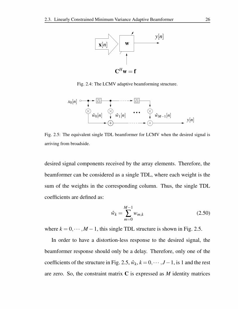
2.3. Linearly Constrained Minimum Variance Adaptive Beamformer 26
x[n]
y[n]
CHw = f
w
Fig. 2.4: The LCMV adaptive beamforming structure.
wM−1[n]
x0[n]
w0[n] w1[n]y[n]
Fig. 2.5: The equivalent single TDL beamformer for LCMV when the desired signal is
arriving from broadside.
desired signal components received by the array elements. Therefore, the
beamformer can be considered as a single TDL, where each weight is the
sum of the weights in the corresponding column. Thus, the single TDL
coefficients are defined as:
wk =M−1
∑m=0
wm,k (2.50)
where k = 0, · · · ,M−1, this single TDL structure is shown in Fig. 2.5.
In order to have a distortion-less response to the desired signal, the
beamformer response should only be a delay. Therefore, only one of the
coefficients of the structure in Fig. 2.5, wk, k = 0, · · · ,J−1, is 1 and the rest
are zero. So, the constraint matrix C is expressed as M identity matrices
2.4. Summary 27
IJ, with size J× J. Thus, C is:
C = [IJ, · · · ,IJ]T . (2.51)
The response vector f is only a delay, so:
f = [0, · · · ,1, · · · ,0]T . (2.52)
After defining C and f, using (2.49), wopt can be obtained and the output
SINR can be calculated using (2.43)–(2.47) from Sec. 2.2.
2.4 Summary
The general area of adaptive wideband beamforming was reviewed in this
chapter. First, the general structure of wideband beamformers using TDLs
was studied and the signal model was introduced which will be used through-
out the thesis. Then, the general structure of the two well-known beam-
formers, namely, RSB and LCMV adaptive beamformers was studied. Un-
der the assumption that the received signals have flat PSDs, the theoretical
values for correlation matrices of the beamformers were calculated. Using
these correlation values the optimum weight vector wopt was calculated for
the beamformers. Since the optimum weight vector wopt and the correla-
tion matrices for desired, interference and the noise for each beamformer
is known, the power of the desired signal Pd , the power of interference
Pi and the power of noise Pn in the output was derived, hence, the output
SINR can be calculated from these values. In the following chapters, a

2.4. Summary 28
method is developed to improve the output SINR by developing a white
noise reduction pre-processing method for different array structures.
Chapter 3
White Noise Reduction for Wideband
Uniform Linear Array Signal
Processing
The most common array structure is the uniform linear array (ULA). The
general idea of the proposed method is presented in this chapter in details
based on a ULA structure for the sensors. Also, the effect of the noise
reduction method on the performance of wideband beamforming and DOA
estimation is shown with simulation. The contents of this chapter has been
published in [50], and parts of the contents is presented at a conference
[51].
3.1 General Structure of the Proposed Method
Consider an M-element ULA, a block diagram for the general structure of
the proposed method is shown in Fig. 3.1. The M received array signals
29
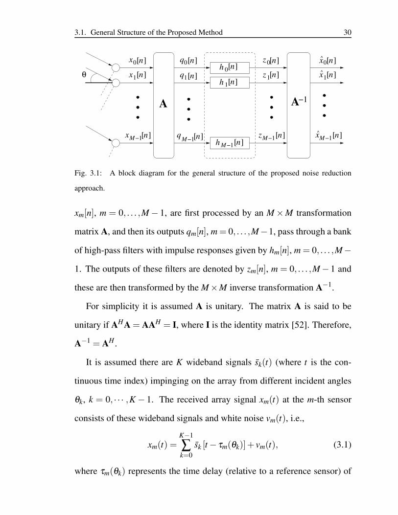
3.1. General Structure of the Proposed Method 30
1θ
−1
n[ ]
n[ ]n[ ]
n[ ]
n[ ]
n[ ]
n[ ]
n[ ]
n[ ]
n[ ]
n[ ]n[ ]
n[ ] n[ ] n[ ]−1M −1M −1M −1M
−1M
^
^
x
x
x
q
q
z
z
x
xh
h
h
A A
0
1
0
1
0
1
q z ^x
1
0 0
Fig. 3.1: A block diagram for the general structure of the proposed noise reduction
approach.
xm[n], m = 0, . . . ,M − 1, are first processed by an M ×M transformation
matrix A, and then its outputs qm[n], m = 0, . . . ,M−1, pass through a bank
of high-pass filters with impulse responses given by hm[n], m = 0, . . . ,M−
1. The outputs of these filters are denoted by zm[n], m = 0, . . . ,M− 1 and
these are then transformed by the M×M inverse transformation A−1.
For simplicity it is assumed A is unitary. The matrix A is said to be
unitary if AHA = AAH = I, where I is the identity matrix [52]. Therefore,
A−1 = AH .
It is assumed there are K wideband signals sk(t) (where t is the con-
tinuous time index) impinging on the array from different incident angles
θk, k = 0, · · · ,K − 1. The received array signal xm(t) at the m-th sensor
consists of these wideband signals and white noise vm(t), i.e.,
xm(t) =K−1
∑k=0
sk [t − τm(θk)]+ vm(t), (3.1)
where τm(θk) represents the time delay (relative to a reference sensor) of
3.1. General Structure of the Proposed Method 31
the k-th impinging signal with the incident angle θk arriving at the m-th
sensor of the array. Taking the first sensor in the array as the reference
point, hence τ0(θk) = 0. So with
sm(t) =K−1
∑k=0
sk [t − τm(θk)] , (3.2)
(3.1) becomes
xm(t) = sm(t)+ vm(t) . (3.3)
With a sampling frequency of fs, the discrete version of the array vector
snapshot is
x[n] = s[n]+v[n] , (3.4)
where
x[n] = [x0[n],x1[n], · · · ,xM−1[n]]T ,
s[n] = [s0[n],s1[n], · · · ,sM−1[n]]T ,
v[n] = [v0[n],v1[n], · · · ,vM−1[n]]T .
Applying the M×M transformation matrix A to the signal vector x[n],
the output signal vector q[n] is obtained as
q[n] = Ax[n], (3.5)
where
q[n] = [q0[n],q1[n], · · · ,qM−1[n]]T .
The element of A at the m-th row and l-th column is denoted by am,l,
i.e., [A]m,l = am,l. Each row vector of A acts as a simple beamformer, and
3.1. General Structure of the Proposed Method 32
its output qm[n] is given by
qm[n] =M−1
∑l=0
am,lxl[n]. (3.6)
The beam response Rm(Ω,θ) of this simple beamformer as a function of
the normalised angular frequency Ω and the DOA angle θ is [38, 53],
Rm(Ω,θ) =M−1
∑l=0
am,le− jlµΩsinθ , (3.7)
where µ = d/cTs and Ω = ωTs, with d being the spacing between the
adjacent sensors, c the wave propagation speed, Ts the sampling period,
and ω the angular frequency of signals.
Since the sampling frequency is fs =1Ts
, the normalised angular fre-
quency is Ω = ωfs= 2π f
fs, where f is the signal frequency. In this thesis, fs
is equal to the Nyquist frequency. Therefore, fs = 2 fmax, where fmax is the
maximum frequency of the signal. So,
Ω =2π f
fs=
2π f
2 fmax=
π f
fmax. (3.8)
Assuming the range of the frequency f is [− fmax : fmax], the range of nor-
malised angular frequency Ω is [−π : π ].
With Ω = µΩsinθ , an alternative representation for Rm(Ω,θ) can be
obtained as follows
Am(Ω) =M−1
∑l=0
am,le− jlΩ, (3.9)
where Ω is representing the spatial frequency of the received signal, Am(Ω)
is the frequency response of the m-th row vector of the M×M transforma-
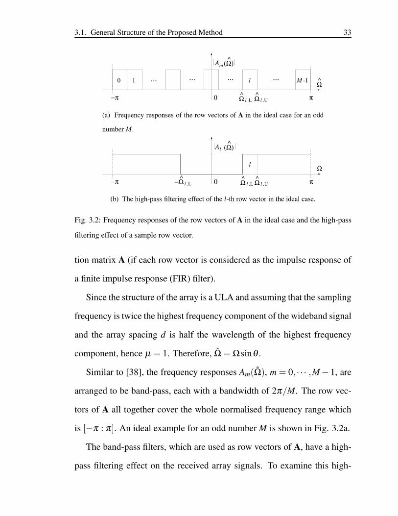
3.1. General Structure of the Proposed Method 33
Ω^
l ,L Ω^
M -1
^(Ω)
... ... ... ...
l ,U−π π
l
0
^Ω
0 1
mA
(a) Frequency responses of the row vectors of A in the ideal case for an odd
number M.
Ω^
l ,L Ω^
l ,U
^(Ω)
−π π
l
0l ,L^
−Ω
Ω
lA
(b) The high-pass filtering effect of the l-th row vector in the ideal case.
Fig. 3.2: Frequency responses of the row vectors of A in the ideal case and the high-pass
filtering effect of a sample row vector.
tion matrix A (if each row vector is considered as the impulse response of
a finite impulse response (FIR) filter).
Since the structure of the array is a ULA and assuming that the sampling
frequency is twice the highest frequency component of the wideband signal
and the array spacing d is half the wavelength of the highest frequency
component, hence µ = 1. Therefore, Ω = Ωsinθ .
Similar to [38], the frequency responses Am(Ω), m = 0, · · · ,M− 1, are
arranged to be band-pass, each with a bandwidth of 2π/M. The row vec-
tors of A all together cover the whole normalised frequency range which
is [−π : π ]. An ideal example for an odd number M is shown in Fig. 3.2a.
The band-pass filters, which are used as row vectors of A, have a high-
pass filtering effect on the received array signals. To examine this high-
3.1. General Structure of the Proposed Method 34
pass behaviour, the l-th row vector is analysed. The frequency response of
this row vector is shown in Fig. 3.2a, which is:
∣
∣Al(Ω)∣
∣=
1, for Ω ∈ [Ωl,L : Ωl,U ]
0, otherwise.
(3.10)
Considering the above frequency response, the received array signal com-
ponents with frequency of Ω ∈ [−Ωl,L : Ωl,L] will not “pass” through this
row vector, since Ω = Ωsinθ does not fall into the passband of [Ωl,L :
Ωl,U ], no matter what value the DOA angle θ takes. Therefore, the fre-
quency range of the output is |Ω| ≥ Ωl,L and the lower bound is determined
by Ωl,L, when Ωl,L > 0. Alternatively, the lower bound is determined by
|Ωl,U |, when Ωl,L < Ωl,U < 0.
As a result, the output spectrum of the directional signal part of ql[n]
corresponding to the l-th row vector will then be high-pass filtered as
shown in Fig. 3.2b. As the noise part in x[n] is spatially white, the out-
put noise spectrum of the row vector is still a constant, covering the whole
spectrum. As shown in Fig. 3.1, the output ql[n], l = 0, · · · ,M − 1, of
each row vector is the input to a corresponding high-pass filter hl[n], l =
0, · · · ,M−1. These high-pass filters should cover the whole bandwidth of
the signal part of the output ql[n] and therefore have the same frequency
response as specified in Fig. 3.2b. As a result, in the ideal case, the high-
pass filters will not have any effect on the signal components and all the
signal components will pass through the high-pass filters without any dis-
tortion. But then the frequency components of the white noise falling into
3.1. General Structure of the Proposed Method 35
the stopband of these high-pass filters will be removed.
The output of the high-pass filters is the convolution of each row vector
output and its corresponding high-pass filter,
z[n] =
z0[n]
...
zM−1[n]
=
q0[n]h0[n]
...
qM−1[n]hM−1[n]
, (3.11)
where denotes the convolution operator.
Considering the noise reduction effect of the high-pass filters, each fil-
ter removes part of the noise except for the filter corresponding to the row
vector with a frequency response covering the zero frequency component,
which should allow all frequencies to pass. Assuming that the size M of the
array is an odd number, from Fig. 3.2, for the first row vector A0(Ω), 2/M
part of the noise passes, while for A1(Ω), 4/M part of the noise passes,
and so on. For the row vector with frequency response covering the zero
frequency, all of the noise will pass. For the row vectors with frequency
responses larger than the zero frequency, the high-pass filters are replicas
of the high-pass filters regarding the row vectors with frequency responses
lower than the zero frequency. Therefore, in the ideal case, the ratio be-
tween the total noise power after and before the processing of the M high-
pass filters can be expressed as
Pvo
Pvi=
1
M
(
1+2
(
2
M+
4
M+ · · ·+ M−1
M
))
, (3.12)
where Pvo is the total noise power at the output of the filters and Pvi is the

3.1. General Structure of the Proposed Method 36
total noise power at their input. Following the same procedure, if the size
of the array is an even number, then this ratio is given by
Pvo
Pvi=
1
M
(
1+2
(
3
M+
5
M+ · · ·+ M−1
M
)
+1
M
)
. (3.13)
As a result,
r(M) =Pvo
Pvi=
M2+2M−12M2 , if M > 1 is odd
M2+2M−22M2 , if M > 2 is even.
(3.14)
When M → ∞, the noise power will be reduced by half in both cases. The
output noise power to input noise power ratio versus the number of array
sensors M is plotted in Fig. 3.3. Since the high-pass filters have no effect
on the signal part, the ratio between the total signal power and the total
noise power is improved by almost 3 dB in the ideal case. For a finite M,
the improvement will be less than 3 dB. For example, when M = 16, it is
about 2.53 dB.
Applying the inverse of the transformation matrix A−1 = AH (with size
M ×M) to z[n], the estimates of the original input sensor signals xm[n],
m = 0, · · · ,M−1 is obtained. In vector form, it is represented as
x[n] = A−1z[n], (3.15)
where x[n] = [x0[n], x1[n], · · · , xM−1[n]]T .
After going through these processing stages, there is no change in the
signal part at the final output xl[n], l = 0, · · · ,M−1 compared to the orig-
inal signal part in xl[n], l = 0, · · · ,M − 1. On the contrary, since A−1 is
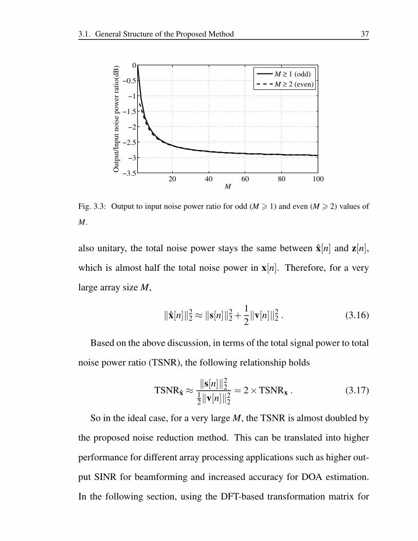
3.1. General Structure of the Proposed Method 37
20 40 60 80 100−3.5
−3
−2.5
−2
−1.5
−1
−0.5
0
M
Outp
ut/
Input
nois
e pow
er r
atio
(dB
)
M ≥ 1 (odd)
M ≥ 2 (even)
Fig. 3.3: Output to input noise power ratio for odd (M > 1) and even (M > 2) values of
M.
also unitary, the total noise power stays the same between x[n] and z[n],
which is almost half the total noise power in x[n]. Therefore, for a very
large array size M,
‖x[n]‖22 ≈ ‖s[n]‖2
2+1
2‖v[n]‖2
2 . (3.16)
Based on the above discussion, in terms of the total signal power to total
noise power ratio (TSNR), the following relationship holds
TSNRx ≈‖s[n]‖2
212‖v[n]‖2
2
= 2×TSNRx . (3.17)
So in the ideal case, for a very large M, the TSNR is almost doubled by
the proposed noise reduction method. This can be translated into higher
performance for different array processing applications such as higher out-
put SINR for beamforming and increased accuracy for DOA estimation.
In the following section, using the DFT-based transformation matrix for
3.2. Analysis Based on the DFT Matrix for ULAs 38
ULAs, the theoretical result for two commonly used beamformers is anal-
ysed to show the performance improvement in the ideal case.
3.2 Analysis Based on the DFT Matrix for ULAs
The transformation matrix A is the most important part of the system. It
should have a full rank so that an inverse transform can be applied at the
end to recover the directional signals. Another key requirement is that
the row vectors have the desired band-pass frequency responses shown
in Fig. 3.2a. So, in general the design of the transformation matrix can
be formulated as a constrained FIR filter design problem. This is similar
to the beamspace transformation problem studied in [54, 55]. As pointed
out there, a prototype low-pass filter could be designed and then it should
be modulated to different frequency bands by a DFT operation or use the
DFT matrix directly. In particular, the DFT matrix is unitary, which will
simplify the theoretical analysis and provide with the crucial insight into
the performance of the proposed structure.
Using the DFT matrix for an M×M transformation A, with γ = e− j(2π/M),
A =1√M
γ0·0 γ0·1 . . . γ0·(M−1)
γ1·0 γ1·1 . . . γ1·(M−1)
......
. . ....
γ(M−1)·0 γ(M−1)·1 . . . γ(M−1)·(M−1)
. (3.18)
Next, an analysis of the signal spectrum based on such a transformation
3.2. Analysis Based on the DFT Matrix for ULAs 39
matrix at different stages of the proposed structure is provided.
3.2.1 Spectrum analysis with DFT matrix
The input-output relationship in the frequency domain based on the DFT
matrix is studied in this section. Taking the discrete-time Fourier transform
(DTFT) of (3.5), (3.11) and (3.15) yields respectively,
q(Ω) = Ax(Ω), (3.19)
z(Ω) = Hq(Ω), (3.20)
x(Ω) = A−1z(Ω), (3.21)
where x(Ω), q(Ω), z(Ω) and x(Ω) are the vectors holding the DTFTs of
the time-domain signal vectors x[n], q[n], z[n] and x[n] respectively. H is
an M ×M real-valued diagonal matrix with its diagonal elements being
the frequency responses Hm(Ω) of the corresponding filters hm[n], m =
0, · · · ,M−1, i.e.,
H =
H0(Ω) 0 . . . 0
0 H1(Ω) . . . 0
......
. . ....
0 0 . . . HM−1(Ω)
. (3.22)
Considering (3.19), (3.20) and (3.21) yields,
x(Ω) = A−1HAx(Ω). (3.23)
From (3.23), the transfer function of the system is:
T = A−1HA =
3.2. Analysis Based on the DFT Matrix for ULAs 40
A−1 1√M
H0(Ω)γ0·0 · · · H0(Ω)γ0·(M−1)
H1(Ω)γ1·0 · · · H1(Ω)γ0·(M−1)
.... . .
...
HM−1(Ω)γ(M−1)·0 · · · HM−1(Ω)γ(M−1)·(M−1)
. (3.24)
Then, all the elements of T (complex-valued, with size M ×M) can be
obtained. Considering the relationship between the terms, a general form
for the elements of T can be derived and the element at the i1-th row and
i2-th column is given by
Ti1,i2 =1
M
M−1
∑l=0
Hlγ−li1γ li2 =
1
M
M−1
∑l=0
Hlγl(i2−i1) . (3.25)
So,
x(Ω) = Tx(Ω). (3.26)
The spectrum of the noise at the output is in interest. The relationship
between the input and output signals’ spectrum is [56],
Sx(Ω) = TT∗(Ω)Sx(Ω), (3.27)
where the asterisk ·∗ denotes the complex conjugate, and Sx(Ω) and
Sx(Ω) are M × M matrices, where each matrix element represents the
cross-spectral density of the two corresponding signals. Sx(i1, i2) is the
(i1, i2)-th element of Sx and it is the cross-spectral density between xi1[n]
and xi2[n]. It can be easily proved that the cross spectral density is equal to
the DTFT of the cross correlation function of the two signals [57]. Then,
Sx(i1, i2) = x∗i1(Ω)xi2(Ω). (3.28)
3.2. Analysis Based on the DFT Matrix for ULAs 41
A detailed proof for (3.28) is provided in the Appendix. Similarly, Sx(i1, i2)=
x∗i1(Ω)xi2(Ω).
Considering the noise part, the spectral density of the white noise is σ2v ,
where σ2v is the variance of the white noise. Since the white noise received
by each array sensor is uncorrelated, the noise spectral density of a sensor
is Sv(i1, i1) = σ2v and the noise cross spectral density between two sensors
is Sv(i1, i2) = 0, the noise cross spectral density is the noise power shared
by a given frequency between two sensors. It needs to be emphasised that,
these assumptions are only valid in the presence of the white noise, and in
other cases these assumptions do not hold. So, the spectrum of the white
noise received by the array is:
Sv(Ω) = σ2v
1 0 · · · 0
0 1 · · · 0
......
. . ....
0 0 · · · 1
= σ2v I , (3.29)
where I is the M×M identity matrix. Therefore, (3.27) can be written as
Sv(Ω) = TT∗(Ω)σ2v I . (3.30)
Sv(Ω) is an M × M complex-valued matrix but with real values on the
diagonal. Each term of Sv(Ω) is given by:
Sv(i1, i2)(Ω) =σ2
v
M
M−1
∑l=0
Ti1,lT∗
i2,l. (3.31)
From (3.25) and (3.31),
Sv(i1, i2)(Ω) =σ2
v
M
M−1
∑l=0
Hl(Ω)e j 2πM(i1−i2)l. (3.32)
3.2. Analysis Based on the DFT Matrix for ULAs 42
−1 −0.5 0 0.5 10
0.2
0.4
0.6
0.8
1
Pow
er S
pec
tral
den
sity
/ σ
2 v
Ω/π
Fig. 3.4: Power spectrum of the output of the noise reduction system with M=16.
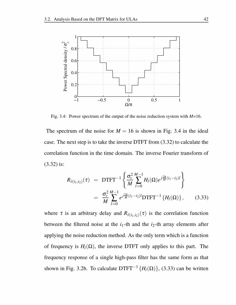
The spectrum of the noise for M = 16 is shown in Fig. 3.4 in the ideal
case. The next step is to take the inverse DTFT from (3.32) to calculate the
correlation function in the time domain. The inverse Fourier transform of
(3.32) is:
Rv(i1,i2)(τ) = DTFT−1
σ2v
M
M−1
∑l=0
Hl(Ω)e j 2πM(i1−i2)l
=σ2
v
M
M−1
∑l=0
e j 2πM(i1−i2)lDTFT−1Hl(Ω) , (3.33)
where τ is an arbitrary delay and Rv(i1,i2)(τ) is the correlation function
between the filtered noise at the i1-th and the i2-th array elements after
applying the noise reduction method. As the only term which is a function
of frequency is Hl(Ω), the inverse DTFT only applies to this part. The
frequency response of a single high-pass filter has the same form as that
shown in Fig. 3.2b. To calculate DTFT−1Hl(Ω), (3.33) can be written
3.3. Performance Analysis of the Proposed Method 43
as
Rv(i1,i2)(τ) =σ2
v
M
M−1
∑l=0
π − Ωl,L
πe j 2π
M(i1−i2)le j
π+Ωl,L2
τ sinc(π − Ωl,L
2τ), (3.34)
where π is the maximum normalised frequency and Ωl,L is the lower bound
frequency of the l-th high-pass filter as was previously shown in Fig. 3.2b.
The correlation values regarding different time delays can be calculated
from (3.34) and will be used to derive the theoretical performance results
for different wideband beamformers.
3.3 Performance Analysis of the Proposed Method for
Adaptive Wideband Beamforming
In this section, the performance of the proposed noise reduction method
for adaptive wideband beamforming is analysed.
3.3.1 Reference signal based adaptive beamformer
For the proposed noise reduction method, in the ideal case the directional
signals (desired and interference) remain intact and only the noise part is
reduced/changed. Then, the total signal vector x corresponding to x after
noise reduction can be expressed as:
x = xd +xi + xv , (3.35)
where xv is the part of x corresponding to the reduced noise after the pro-
posed processing.
3.3. Performance Analysis of the Proposed Method 44
Similarly, the correlation matrices ΦΦΦd and ΦΦΦi will remain the same af-
ter noise reduction, but the correlation matrix for the noise part will be
changed to ΦΦΦv with size MJ×MJ. Then, the MJ ×MJ correlation matrix
ΦΦΦx after noise reduction can be expressed as:
ΦΦΦx =ΦΦΦd +ΦΦΦi +ΦΦΦv . (3.36)
ΦΦΦv can be obtained from (3.34) and partition it into M×M submatrices
(each submatrix is J× J),
ΦΦΦv =
ΦΦΦv0,0· · · ΦΦΦv0,M−1
.... . .
...
ΦΦΦvM−1,0· · · ΦΦΦvM−1,M−1
. (3.37)
where ΦΦΦvi1,i2= E
[
x∗vi1xT
vi2
]
. The delay between two adjacent taps in a TDL
is T0 =πr
2Ω0, where Ω0 is the normalised centre frequency and r is the num-
ber of quarter-wave delays in T0 at frequency Ω0. Hence the delay between
the i-th and the k-th taps is τ = (i− k)T0. Therefore, the correlation value[
ΦΦΦvi1,i2
]
i,kbetween the noise (after the proposed processing) at the i-th tap
of the i1-th element and that at the k-th tap of the i2-th element is given by
[
ΦΦΦvi1,i2
]
i,k= E
[
v∗i1,i[n]vi2,k[n]]
= Rv(i1,i2) [(i− k)T0] . (3.38)
From (3.34) and (3.38),
[
ΦΦΦvi1,i2
]
i,k=
σ2v
M
M−1
∑l=0
π − Ωl,L
πe j 2π
M(i1−i2)le j
π+Ωl,L2
(i−k)T0
× sinc(π − Ωl,L
2(i− k)T0) .
(3.39)
3.3. Performance Analysis of the Proposed Method 45
Now all the correlation values required for calculating the wopt in (2.6)
is determined and the beamformer output y[n] is
y[n] = wTopt x , (3.40)
with its power given by
P =1
2E[
‖y[n]‖2]
=1
2wH
optΦΦΦxwopt . (3.41)
The output SINR is given by
SINR =Pd
Pi +Pv, (3.42)
where
Pd =1
2wH
optΦΦΦdwopt , (3.43)
Pi =1
2wH
optΦΦΦiwopt , (3.44)
Pv =1
2wH
optΦΦΦvwopt . (3.45)
3.3.2 Linearly constrained minimum variance adaptive beamformer
In practice, the reference signal assumed in Section 2.2 may be unavail-
able. However, when some information on the DOAs as well as the band-
width limits of the desired signal and/or the interferences is available, the
LCMV beamformer can be employed for effective beamforming [2, 49].
The LCMV beamformer is formulated as follows (based on the recovered
signal x after the proposed noise reduction method),
minw
wHΦΦΦxw subject to CHw = f , (3.46)
3.4. Compressive Sensing Based DOA Estimation 46
where w and ΦΦΦx are defined as before in Section 2.2 and Section 3.3.1,
C is the MJ × J constraint matrix and f is the J × 1 response vector. The
solution to (3.46) can be obtained using the Lagrange multipliers method,
wopt =ΦΦΦ−1x C(CHΦΦΦ−1
x C)−1f . (3.47)
Suppose the desired signal comes from the broadside, i.e., θd = 0.
Then, C and f have a very simple form, and they are same as (2.51) and
(2.52). With the optimal weight vector determined, the output SINR can
be obtained as in Section 2.2.
3.4 Compressive Sensing Based DOA Estimation
To further demonstrate the improved array processing performance with an
improved TSNR, the effect of the developed method on the performance
of the wideband DOA estimation problem is considered in this section by
employing a compressive sensing based method.
3.4.1 Introduction to compressive sensing
The DOA estimation techniques are widely used for different applications
such as radars. Most of the DOA estimation scenarios are sparse, since
only a small fraction of the azimuth-range or the elevation-range cells are
occupied by objects of interest. Therefore, compressive sensing (CS) [58,
59] is a suitable approach to solve the DOA estimation problem.
3.4. Compressive Sensing Based DOA Estimation 47
By employing the compressive sensing it is possible to reconstruct a
sparse signal f from an under-determined linear system of equations Bf =
g. Assuming f is a sparse vector with length L, the number of non-zero
elements of f satisfies, ‖ f‖0 ≪ L, where ‖ · ‖0 denotes the l0 norm, which
is the number of non-zero elements of a vector. Assume B is a K × L
matrix of rank K, with K < L, so B is under-determined. f is considered to
be sparse, hence, it can be computed from,
minf
‖f‖0
subject to Bf = g ,
(3.48)
which is a non-deterministic polynomial-time (NP) hard problem. There-
fore, solving (3.48) is not practically feasible. By using convex relax-
ation [60], also known as Basis Pursuit [61], the l0 norm in (3.48) is relaxed
by l1 norm. So, (3.48) is written as,
minf
‖f‖1
subject to Bf = g ,
(3.49)
where ‖ ·‖1 denotes the l1 norm. (3.49) can be solved by convex optimiza-
tion methods [62]. Two conditions have to be satisfied, so that (3.49) can
be solvable. One condition is that B must satisfy the isotropy property,
which states that the components of each row of B have unit variance and
they are uncorrelated. Another condition is that B should have a small co-
herence. The coherence is defined as the maximum inner product between
normalised columns of B [63].
3.4. Compressive Sensing Based DOA Estimation 48
The compressive sensing based DOA estimation method adopted in this
chapter is a direct adaptation and extension of the method developed in [29]
and [32] for co-prime arrays.
3.4.2 Signal model for DOA estimation
First, for the received vector signal in (3.4), it is divided into P non-
overlapping groups with length L, and an L-point DFT is then applied. The
l-th frequency bin samples of the p-th group are placed into one vector as:
X[l, p] = [X0[l, p],X1[l, p], · · · ,XM−1[l, p]]T , (3.50)
where
Xn[l, p] =L−1
∑i=0
xn[Lp+ i]e− j 2πL
il, (3.51)
with p = 0, · · · ,P−1 and l = 0, · · · ,L−1.
Define Sk[l, p] and Vm[l, p] as the DFT of the p-th group impinging sig-
nals sk[n] and noise vm[n], respectively. S[l, p] =[
S0[l, p], · · · , SK−1[l, p]]T
is a column vector holding signals from the l-th frequency bin, and V[l, p] =
[V0[l, p], · · · ,VM−1[l, p]]T is the column noise vector of the array. Then, the
output signal model in the DFT domain can be expressed as:
X[l, p] = D(l,θ)S[l, p]+V[l, p], (3.52)
where D(l,θ) = [d(l,θ0), ...,d(l,θK−1)] is the steering matrix at frequency
Ωl corresponding to the l-th frequency bin. The column vector d(l,θk) is
the steering vector at frequency Ωl and angle θk, which is given by
d(l,θk) =
[
1, e− j d
cTsΩl sinθk , · · · , e
− j(M−1)d
cTsΩl sinθk
]
. (3.53)
3.4. Compressive Sensing Based DOA Estimation 49
By considering each frequency bin of interest separately, (3.52) is a nar-
rowband signal model.
3.4.3 Generating the virtual array
The auto-correlation matrix of the observed array vector X[l, p] is:
Rxx[l] = E
X[l, p]XH [l, p]
=K−1
∑k=0
σ2k [l]d(l,θk)d
H(l,θk)+σ2v [l]IM ,
(3.54)
where IM is the M×M identity matrix. σ2k [l] represents the power of the k-
th impinging signal of the l-th frequency bin and σ2v [l] is the corresponding
noise power. In practical applications, it can be assumed that,
Rxx[l] ≈1
P
P−1
∑p=0
X[l, p] ·XH [l, p], (3.55)
and it is assumed that the directional signals are wide-sense stationary.
Vectorising Rxx[l] yields:
u[l] = vecRxx= D[l]s[l]+σ2v IM , (3.56)
where D[l] = [d(l,θ0), · · · , d(l,θK−1)], d(l,θk) = d∗(l,θk)⊗d(l,θk) (⊗ is
the Kronecker product), and s[l] = σ20 [l],σ
21 [l], · · · , σ2
K−1[l]T . IM is an
M2 × 1 column vector obtained by vectorising the identity matrix IM. Eq.
(3.56) characterises a virtual array with D[l] and s[l] as its steering matrix
and impinging signal vector, respectively. Eq. (3.56) can be reduced to:
u[l] = D[l]s[l], (3.57)
where D[l] =
[
D[l], IM
]
and s =[
sT [l],σ2v [l]
]T.
3.4. Compressive Sensing Based DOA Estimation 50
3.4.4 Narrowband DOA estimation
For the l-th frequency, with a search grid of Kg potential arriving angles
(θg,0, · · · ,θg,Kg−1) , the steering matrix is
Dg[l] =[
d(l,θg,0), · · · , d(l,θg,Kg−1)]
. (3.58)
Constructing a column vector sg[l] consisting of Kg elements, with each
representing a potential arriving signal, yields
Dg[l] =
[
Dg[l], IM
]
; sg[l] =[
sg[l],σ2v [l]
]T
. (3.59)
Since noise power is not known, σ2v [l] is also considered to be a variable.
In [29], a compressive sensing based DOA estimation was proposed for co-
prime arrays, which can be applied directly for the ULA case. Therefore,
for the l-th frequency bin, the narrowband DOA estimation is formulated
as:
minsg[l]
∥
∥sg[l]∥
∥
1
subject to∥
∥u[l]− Dg[l]s
g[l]
∥
∥
2≤ ε ,
(3.60)
where ε denote the error bound.
3.4.5 Wideband DOA estimation
The narrowband DOA estimation in (3.60) can be used for wideband case
by applying the estimation to each frequency bin, and then averaging the
results.
For each frequency bin, the impinging signals have the same spatial
characteristics, although the amount of power regarding each DOA might
3.4. Compressive Sensing Based DOA Estimation 51
be different. This is known as the group sparsity concept [64, 65]. There-
fore, a more effective alternative is to apply the DOA estimation over the
frequency range of interest simultaneously.
It is assumed Q frequency bins are covering the frequency range of
interest in the DFT domain, where Q ≤ L, and the same search grid Kg is
assumed for each frequency bin lq, 0 ≤ q ≤ Q−1.
Two matrices should be constructed here, a block diagonal matrix Dg
using Dg[lq],
Dg = blkdiagDg[l0],D
g[l1], · · · ,D
g[lQ−1] , (3.61)
and a (Kg+1)×Q matrix R using sg[lq] with R=[
sg[l0], sg[l1], · · · , sg[lQ−1]
]
.
Then, the following wideband virtual array model u= Dgr can be obtained,
where u =[
uT [l0], · · · ,uT [lQ−1]]T
and r = vec(R) is a (Kg+1) ·Q×1 col-
umn vector by vectorising R. The row vector rk, 0 ≤ k ≤ Kg, is used to
represent k-th row of matrix R. Then, a new (Kg +1)×1 column vector r
is formed based on the l2 norm of rk, 0 ≤ k ≤ Kg, as given below
r =[
‖r0‖2 ,‖r1‖2 , · · · ,∥
∥rKg
∥
∥
2
]T. (3.62)
Finally, the group sparsity based wideband DOA estimation is formulated
as follows
minr
‖r‖1
subject to∥
∥u− Dgr∥
∥
2≤ ε .
(3.63)
The problem in (3.63) can be solved using CVX, a software package for
specifying and solving convex programs [66,67]. The steps for calculating
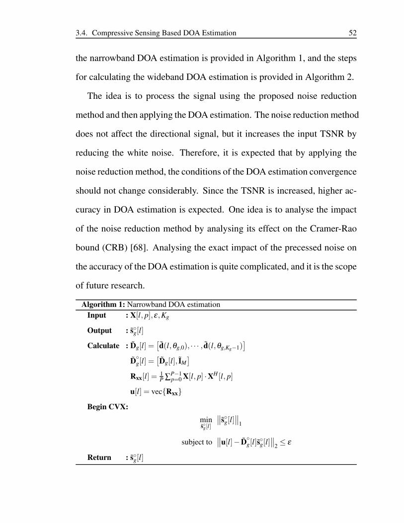
3.4. Compressive Sensing Based DOA Estimation 52
the narrowband DOA estimation is provided in Algorithm 1, and the steps
for calculating the wideband DOA estimation is provided in Algorithm 2.
The idea is to process the signal using the proposed noise reduction
method and then applying the DOA estimation. The noise reduction method
does not affect the directional signal, but it increases the input TSNR by
reducing the white noise. Therefore, it is expected that by applying the
noise reduction method, the conditions of the DOA estimation convergence
should not change considerably. Since the TSNR is increased, higher ac-
curacy in DOA estimation is expected. One idea is to analyse the impact
of the noise reduction method by analysing its effect on the Cramer-Rao
bound (CRB) [68]. Analysing the exact impact of the precessed noise on
the accuracy of the DOA estimation is quite complicated, and it is the scope
of future research.
Algorithm 1: Narrowband DOA estimation
Input : X[l, p],ε,Kg
Output : sg[l]
Calculate : Dg[l] =[
d(l,θg,0), · · · , d(l,θg,Kg−1)]
Dg[l] =
[
Dg[l], IM
]
Rxx[l] =1P ∑P−1
p=0 X[l, p] ·XH [l, p]
u[l] = vecRxx
Begin CVX:
minsg[l]
∥
∥sg[l]∥
∥
1
subject to∥
∥u[l]− Dg[l]s
g[l]
∥
∥
2≤ ε
Return : sg[l]
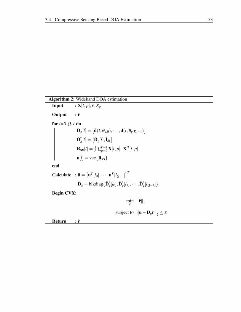
3.4. Compressive Sensing Based DOA Estimation 53
Algorithm 2: Wideband DOA estimation
Input : X[l, p],ε,Kg
Output : r
for l=0:Q-1 do
Dg[l] =[
d(l,θg,0), · · · , d(l,θg,Kg−1)]
Dg[l] =
[
Dg[l], IM
]
Rxx[l] =1P ∑P−1
p=0 X[l, p] ·XH [l, p]
u[l] = vecRxxend
Calculate : u =[
uT [l0], · · · ,uT [lQ−1]]T
Dg = blkdiagDg[l0], D
g[l1], · · · , D
g[lQ−1]
Begin CVX:
minr
‖r‖1
subject to∥
∥u− Dgr∥
∥
2≤ ε
Return : r
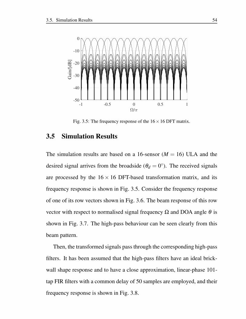
3.5. Simulation Results 54
-1 -0.5 0 0.5 1
/
-50
-40
-30
-20
-10
0
Gai
n/[
dB
]
Fig. 3.5: The frequency response of the 16×16 DFT matrix.
3.5 Simulation Results
The simulation results are based on a 16-sensor (M = 16) ULA and the
desired signal arrives from the broadside (θd = 0). The received signals
are processed by the 16× 16 DFT-based transformation matrix, and its
frequency response is shown in Fig. 3.5. Consider the frequency response
of one of its row vectors shown in Fig. 3.6. The beam response of this row
vector with respect to normalised signal frequency Ω and DOA angle θ is
shown in Fig. 3.7. The high-pass behaviour can be seen clearly from this
beam pattern.
Then, the transformed signals pass through the corresponding high-pass
filters. It has been assumed that the high-pass filters have an ideal brick-
wall shape response and to have a close approximation, linear-phase 101-
tap FIR filters with a common delay of 50 samples are employed, and their
frequency response is shown in Fig. 3.8.
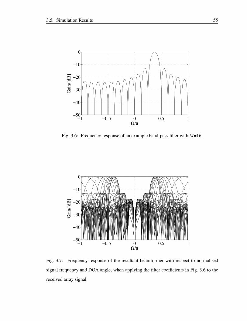
3.5. Simulation Results 55
−1 −0.5 0 0.5 1−50
−40
−30
−20
−10
0
Ω/π
Gai
n/[
dB
]
Fig. 3.6: Frequency response of an example band-pass filter with M=16.
−1 −0.5 0 0.5 1−50
−40
−30
−20
−10
0
Ω/π
Gai
n/[
dB
]
Fig. 3.7: Frequency response of the resultant beamformer with respect to normalised
signal frequency and DOA angle, when applying the filter coefficients in Fig. 3.6 to the
received array signal.
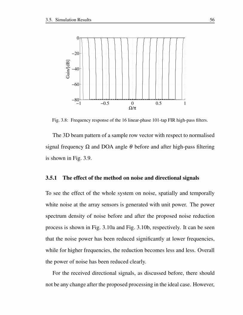
3.5. Simulation Results 56
−1 −0.5 0 0.5 1−80
−60
−40
−20
0
Ω/π
Gai
n/[
dB
]
Fig. 3.8: Frequency response of the 16 linear-phase 101-tap FIR high-pass filters.
The 3D beam pattern of a sample row vector with respect to normalised
signal frequency Ω and DOA angle θ before and after high-pass filtering
is shown in Fig. 3.9.
3.5.1 The effect of the method on noise and directional signals
To see the effect of the whole system on noise, spatially and temporally
white noise at the array sensors is generated with unit power. The power
spectrum density of noise before and after the proposed noise reduction
process is shown in Fig. 3.10a and Fig. 3.10b, respectively. It can be seen
that the noise power has been reduced significantly at lower frequencies,
while for higher frequencies, the reduction becomes less and less. Overall
the power of noise has been reduced clearly.
For the received directional signals, as discussed before, there should
not be any change after the proposed processing in the ideal case. However,
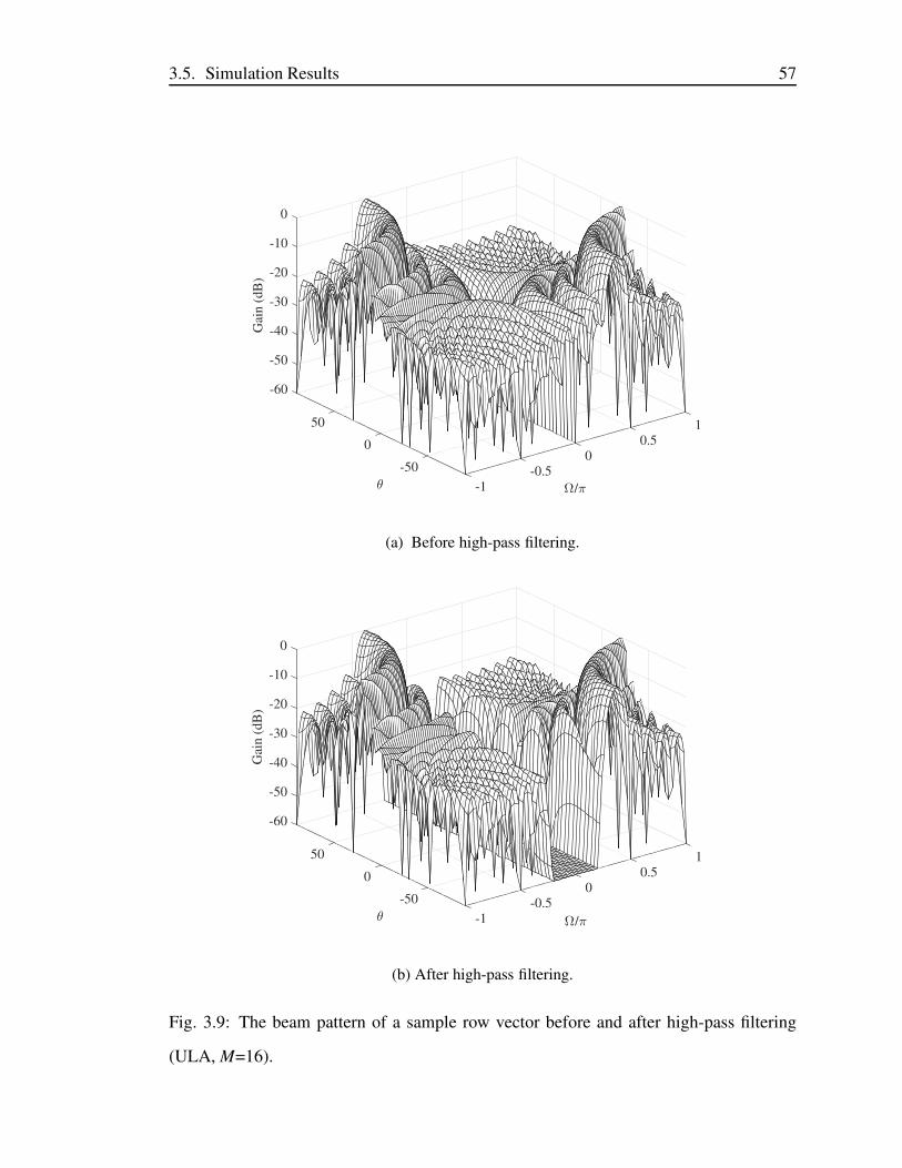
3.5. Simulation Results 57
-60
-50
-40
50 1
-30
Gai
n (
dB
) -20
0.50
-10
/
0
0-50 -0.5
-1
(a) Before high-pass filtering.
-60
-50
-40
50 1
-30
Gai
n (
dB
) -20
0.50
-10
/
0
0-50 -0.5
-1
(b) After high-pass filtering.
Fig. 3.9: The beam pattern of a sample row vector before and after high-pass filtering
(ULA, M=16).
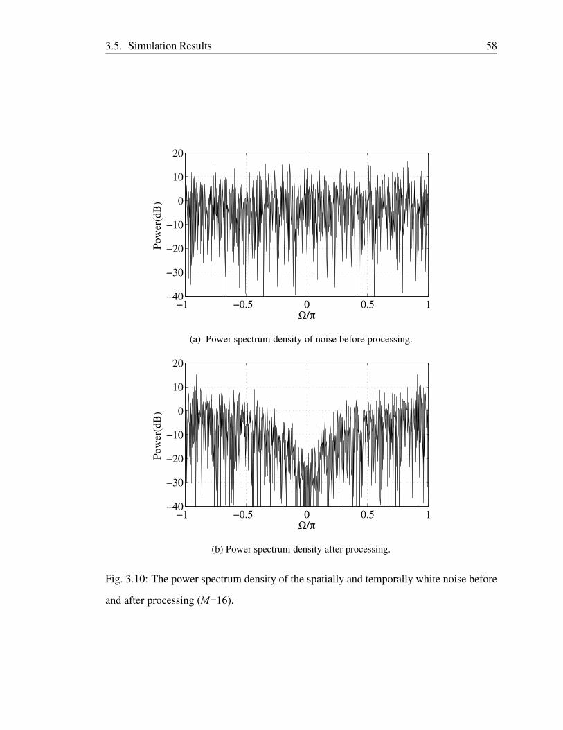
3.5. Simulation Results 58
−1 −0.5 0 0.5 1−40
−30
−20
−10
0
10
20
Ω/π
Pow
er(d
B)
(a) Power spectrum density of noise before processing.
−1 −0.5 0 0.5 1−40
−30
−20
−10
0
10
20
Ω/π
Pow
er(d
B)
(b) Power spectrum density after processing.
Fig. 3.10: The power spectrum density of the spatially and temporally white noise before
and after processing (M=16).
3.5. Simulation Results 59
the response of the row vectors of the transformation is not ideal and as a
result, a small amount of the directional signals will exist at the lower side-
lobe region and it will be removed by the following high-pass filters.
In order to show this effect, a wideband signal with unit power is applied
to the array from the broadside. The number of signals N sampled in the
time domain at each sensor is 32768. The MSE for the directional signals
before and after the proposed processing is calculated by,
MSE =1
MN
M−1
∑m=0
N−1
∑n=0
(xm[n]− xm[n])2 . (3.64)
The results for different array size (M) are shown in Table 3.1, where it
can be seen that the effect on the directional signal can be ignored for
M > 16. Therefore, the directional signal is recovered with less distortion
by increasing M, since by increasing the array size, less signal is available
in the side-lobes which will be removed by the corresponding high-pass
filters.
The output noise power Pvo to the input noise power Pvi is calculated
and presented in Table 3.2. It can be seen that the power ratio which is pre-
sented in (3.14) is getting closer to the ideal case of -3 dB, as M increases.
Therefore, larger array size M results in having a better recovery of the
directional signal, and having a more effective white noise reduction.
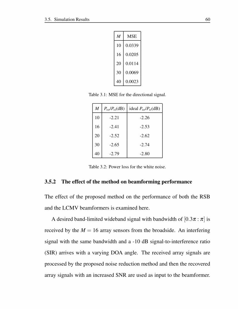
3.5. Simulation Results 60
M MSE
10 0.0339
16 0.0205
20 0.0114
30 0.0069
40 0.0023
Table 3.1: MSE for the directional signal.
M Pvo/Pvi(dB) ideal Pvo/Pvi(dB)
10 -2.21 -2.26
16 -2.41 -2.53
20 -2.52 -2.62
30 -2.65 -2.74
40 -2.79 -2.80
Table 3.2: Power loss for the white noise.
3.5.2 The effect of the method on beamforming performance
The effect of the proposed method on the performance of both the RSB
and the LCMV beamformers is examined here.
A desired band-limited wideband signal with bandwidth of [0.3π : π ] is
received by the M = 16 array sensors from the broadside. An interfering
signal with the same bandwidth and a -10 dB signal-to-interference ratio
(SIR) arrives with a varying DOA angle. The received array signals are
processed by the proposed noise reduction method and then the recovered
array signals with an increased SNR are used as input to the beamformer.
3.5. Simulation Results 61
The input SNR is 0 dB and the TDL length is J = 100.
The output SINR performances of both beamformers with and without
the proposed pre-processing are compared in Fig. 3.11 as a function of the
DOA angle θi of the interfering signal, where the theoretical value is based
on the result derived in Sec. 3.3. It can be seen that the simulation result
matches the theoretical one very well. With the change of the direction of
the interfering signal, except for the region where DOA of the interfering
signal is very close to the desired signal, an almost constant improvement
of about 2 dB can be observed.
It is also important to analyse how the output SINR performance of
the proposed method varies with different input SNRs. Seven interfering
signals are applied to the system, each with a -10 dB input SIR, and their
DOAs are θi = 10,20,30,40,50,60 and 70, respectively. All the
other settings are the same as before. The results are shown in Fig. 3.12. As
expected, a higher output SINR has been achieved by the proposed method
for both beamformers especially when the input SNR is larger than -10 dB
and generally the improvement becomes larger when input SNR increases.
In general, the theoretical results should be the best one, but it can be
seen in Fig. 3.11 and Fig. 3.12 that the simulated results are better than the
theoretical results. The reason is that the band-pass response of the row
vectors of the transformation is not ideal and therefore, the directional sig-
nal components which are available in the lower side-lobes are removed
by the high-pass filters. So, the interfering signals are going to be slightly
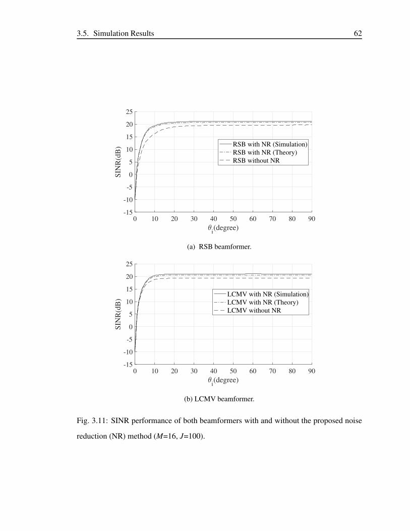
3.5. Simulation Results 62
0 10 20 30 40 50 60 70 80 90
i(degree)
-15
-10
-5
0
5
10
15
20
25S
INR
(dB
) RSB with NR (Simulation)
RSB with NR (Theory)
RSB without NR
(a) RSB beamformer.
0 10 20 30 40 50 60 70 80 90
i(degree)
-15
-10
-5
0
5
10
15
20
25
SIN
R(d
B)
LCMV with NR (Simulation)
LCMV with NR (Theory)
LCMV without NR
(b) LCMV beamformer.
Fig. 3.11: SINR performance of both beamformers with and without the proposed noise
reduction (NR) method (M=16, J=100).
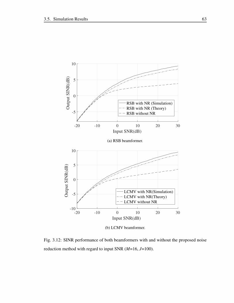
3.5. Simulation Results 63
-20 -10 0 10 20 30
Input SNR(dB)
-5
0
5
10O
utp
ut
SIN
R(d
B)
RSB with NR (Simulation)
RSB with NR (Theory)
RSB without NR
(a) RSB beamformer.
-20 -10 0 10 20 30
Input SNR(dB)
-10
-5
0
5
10
Outp
ut
SIN
R(d
B)
LCMV with NR(Simulation)
LCMV with NR(Theory)
LCMV without NR
(b) LCMV beamformer.
Fig. 3.12: SINR performance of both beamformers with and without the proposed noise
reduction method with regard to input SNR (M=16, J=100).
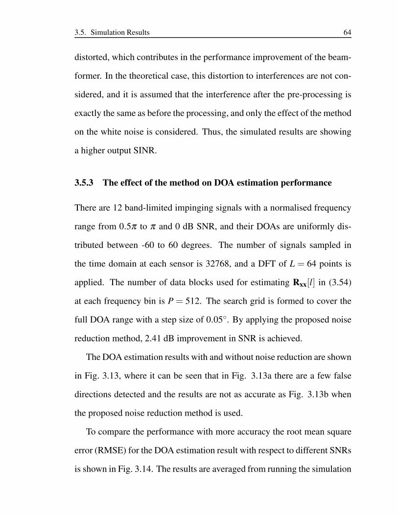
3.5. Simulation Results 64
distorted, which contributes in the performance improvement of the beam-
former. In the theoretical case, this distortion to interferences are not con-
sidered, and it is assumed that the interference after the pre-processing is
exactly the same as before the processing, and only the effect of the method
on the white noise is considered. Thus, the simulated results are showing
a higher output SINR.
3.5.3 The effect of the method on DOA estimation performance
There are 12 band-limited impinging signals with a normalised frequency
range from 0.5π to π and 0 dB SNR, and their DOAs are uniformly dis-
tributed between -60 to 60 degrees. The number of signals sampled in
the time domain at each sensor is 32768, and a DFT of L = 64 points is
applied. The number of data blocks used for estimating Rxx[l] in (3.54)
at each frequency bin is P = 512. The search grid is formed to cover the
full DOA range with a step size of 0.05. By applying the proposed noise
reduction method, 2.41 dB improvement in SNR is achieved.
The DOA estimation results with and without noise reduction are shown
in Fig. 3.13, where it can be seen that in Fig. 3.13a there are a few false
directions detected and the results are not as accurate as Fig. 3.13b when
the proposed noise reduction method is used.
To compare the performance with more accuracy the root mean square
error (RMSE) for the DOA estimation result with respect to different SNRs
is shown in Fig. 3.14. The results are averaged from running the simulation
3.5. Simulation Results 65
−80 −60 −40 −20 0 20 40 60 800
0.2
0.4
0.6
0.8
1
θ: Degrees
Norm
alis
ed S
pec
trum
(a) Without white noise reduction.
−80 −60 −40 −20 0 20 40 60 800
0.2
0.4
0.6
0.8
1
θ: Degrees
Norm
alis
ed S
pec
trum
(b) With white noise reduction.
Fig. 3.13: DOA estimation results with and without the proposed white noise reduction.
100 times. It can be clearly seen that using the developed noise reduction
method, the DOA estimation result has been improved significantly over
the whole considered input SNR range.
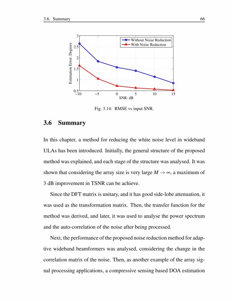
3.6. Summary 66
−10 −5 0 5 10 150.5
1
1.5
2
2.5
3
SNR: dB
Est
imat
ion
Err
or:
Deg
rees
Without Noise Reduction
With Noise Reduction
Fig. 3.14: RMSE vs input SNR.
3.6 Summary
In this chapter, a method for reducing the white noise level in wideband
ULAs has been introduced. Initially, the general structure of the proposed
method was explained, and each stage of the structure was analysed. It was
shown that considering the array size is very large M → ∞, a maximum of
3 dB improvement in TSNR can be achieve.
Since the DFT matrix is unitary, and it has good side-lobe attenuation, it
was used as the transformation matrix. Then, the transfer function for the
method was derived, and later, it was used to analyse the power spectrum
and the auto-correlation of the noise after being processed.
Next, the performance of the proposed noise reduction method for adap-
tive wideband beamformers was analysed, considering the change in the
correlation matrix of the noise. Then, as another example of the array sig-
nal processing applications, a compressive sensing based DOA estimation
3.6. Summary 67
for was reviewed.
In the simulation section, the effect of the method on the directional sig-
nal, and white noise presented. Then, the SINR performance of the RSB
and LCMV beamformers with and without the noise reduction method was
demonstrated, which confirmed the increased output SINR for beamform-
ers using the proposed method. Also, simulation results showed an im-
provement in the accuracy of the compressive sensing based DOA estima-
tion.
Chapter 4
Extension of the Noise Reduction
Method for Non-uniform Linear Arrays
In Chapter 3, a method was developed for reducing the effect of white noise
in wideband ULAs via a combination of a judiciously designed transforma-
tion followed by high-pass filters to improve the performance for wideband
beamforming and DOA estimation. In this chapter, that idea is extended
to non-uniform linear arrays (NLAs) and as a result, the transformation is
re-designed using the least squares method to adjust the noise reduction
method for the non-uniform sensor layout of NLAs.
To make sure the transformation is invertible, a prototype filter is first
designed and then modulated to different subbands to cover the full nor-
malised frequency band from −π to π . The diagonal loading method is
used to keep the condition number to a low level [69]. Similar to the ULA
case, the overall SNR of the system can be improved by up to 3 dB, which
then leads to performance enhancement for beamforming as demonstrated
68
4.1. The Proposed White Noise Reduction for Non-uniform Linear Arrays 69
using two well-known adaptive beamformers, namely the RSB [70,71] and
the LCMV beamformers [2, 49].
The contents of this chapter is published in [50] and is also presented at
a conference [72].
4.1 The Proposed White Noise Reduction for Non-uniform
Linear Arrays
The general structure of the proposed method for NLAs is same as the
general structure for ULAs, as presented in Fig. 3.1. M array signals
xm[n],m = 0, · · · ,M − 1, are received by the NLA sensors. Then, the re-
ceived array signals are transformed by an M×M transformation A. Next,
the transformed signals qm[n],m = 0, · · · ,M − 1, are passed through the
corresponding high-pass filters hm[n],m = 0, · · · ,M−1. Finally, the high-
pass filtered signals zm[n],m = 0, · · · ,M − 1 are block-transformed by the
inverse of the transformation A−1.
The signal model is similar to the ULA case, and it can be presented
by (3.1)–(3.4). By applying the M×M transformation to the signal vector
x[n], the output signal vector is obtained as (3.5). Each row vector of A acts
as a simple beamformer, with its output same as (3.6). The beam response
Rm(Ω,θ) of this beamformer for the NLA structure is given by:
Rm(Ω,θ) =M−1
∑l=0
am,le− j
dlcTs
(Ωsinθ) = Am(Ωsinθ), (4.1)
where dl is the spacing between the zero-th sensor and the l-th sensor
4.1. The Proposed White Noise Reduction for Non-uniform Linear Arrays 70
(where d0=0). Therefore, considering Ω = Ωsinθ ,
Am(Ω) =M−1
∑l=0
am,le− j
dlcTs
Ω, (4.2)
where Am(Ω) is the frequency response of the m-th row vector of the trans-
formation matrix A, considering each row vector as the impulse response
of an FIR filter. The frequency responses Am(Ω),m = 0, · · · ,M−1, are set
to have band-pass characteristics, each with a bandwidth of 2π/M. Over-
all, the row vectors of A cover the entire normalised frequency band of
[−π : π ].
By considering the entire range of the DOA θ of the received sig-
nals, the row vectors of A have high-pass filtering behaviour as explained
in Sec. 3.1. According to the general structure in Fig. 3.1, each high-
pass filter hl[n], l = 0, · · · ,M − 1, processes its corresponding input ql[n],
l = 0, · · · ,M−1. The high-pass filters have the same high-pass frequency
response as their corresponding row vectors of the transformation A, and
they cover the entire bandwidth of the directional signal. Therefore, in the
ideal case, the directional signal is not affected by any distortion after be-
ing processed by the high-pass filters. On the contrary, the high-pass filters
remove parts of the white noise which fall into their stop-band.
The output of the aforementioned high-pass filters which is denoted
by zl[n], l = 0, · · · ,M− 1, is then processed by the inverse transformation
A−1, and the original array signals will be recovered without any distor-
tion in the ideal case, while the noise power will be reduced leading to an
4.2. Least Squares Based Design for the Transformation Matrix 71
improved overall SNR. Following the same analysis for the ULA, as dis-
cussed in Sec. 3.1, when A is unitary, up to 3 dB total SNR improvement
can be achieved by the proposed method. Although, in practice, the TSNR
improvement will be less than 3 dB, due to limited number of sensors and
difficulty in designing a unitary transformation matrix with the required
band-pass responses for the NLA case.
The transformation matrix A is required to be unitary to make sure that
the row vectors of both A and A−1 have unity norm and preserve the signal
power after transforming the signal and also after transforming the signal
back. If the transformation is not unitary, the noise might be amplified sig-
nificantly during the process, even if some of it has been removed by high-
pass filters, which subsequently leads to a reduced output SNR. Moreover,
a unitary transformation ensures that A is of full rank.
In the next section, the design of the transformation for NLAs is pre-
sented, with required band-pass characteristics.
4.2 Least Squares Based Design for the Transformation
Matrix
As an example for a unitary matrix with a good band-pass response, the
DFT matrix in the ULA case is considered in this section. However, the
DFT matrix is not applicable for the NLA case, since it does not have a
uniform spacing, and the resultant beams by each row vector of such a
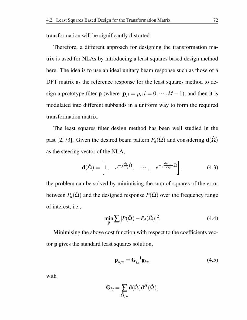
4.2. Least Squares Based Design for the Transformation Matrix 72
transformation will be significantly distorted.
Therefore, a different approach for designing the transformation ma-
trix is used for NLAs by introducing a least squares based design method
here. The idea is to use an ideal unitary beam response such as those of a
DFT matrix as the reference response for the least squares method to de-
sign a prototype filter p (where [p]l = pl, l = 0, · · · ,M − 1), and then it is
modulated into different subbands in a uniform way to form the required
transformation matrix.
The least squares filter design method has been well studied in the
past [2, 73]. Given the desired beam pattern Pd(Ω) and considering d(Ω)
as the steering vector of the NLA,
d(Ω) =
[
1, e− j
d1cTs
Ω, · · · , e− j
dM−1cTs
Ω
]
, (4.3)
the problem can be solved by minimising the sum of squares of the error
between Pd(Ω) and the designed response P(Ω) over the frequency range
of interest, i.e.,
minp
∑ |P(Ω)−Pd(Ω)|2. (4.4)
Minimising the above cost function with respect to the coefficients vec-
tor p gives the standard least squares solution,
popt = G−1ls gls, (4.5)
with
Gls = ∑Ωpb
d(Ω)dH(Ω),
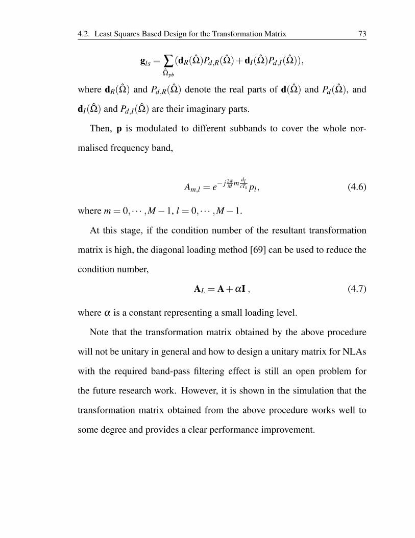
4.2. Least Squares Based Design for the Transformation Matrix 73
gls = ∑Ωpb
(dR(Ω)Pd,R(Ω)+dI(Ω)Pd,I(Ω)),
where dR(Ω) and Pd,R(Ω) denote the real parts of d(Ω) and Pd(Ω), and
dI(Ω) and Pd,I(Ω) are their imaginary parts.
Then, p is modulated to different subbands to cover the whole nor-
malised frequency band,
Am,l = e− j 2π
Mm
dlcTs pl, (4.6)
where m = 0, · · · ,M−1, l = 0, · · · ,M−1.
At this stage, if the condition number of the resultant transformation
matrix is high, the diagonal loading method [69] can be used to reduce the
condition number,
AL = A+αI , (4.7)
where α is a constant representing a small loading level.
Note that the transformation matrix obtained by the above procedure
will not be unitary in general and how to design a unitary matrix for NLAs
with the required band-pass filtering effect is still an open problem for
the future research work. However, it is shown in the simulation that the
transformation matrix obtained from the above procedure works well to
some degree and provides a clear performance improvement.
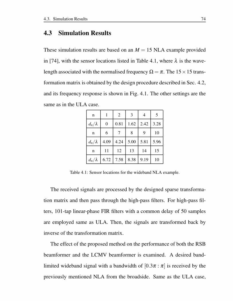
4.3. Simulation Results 74
4.3 Simulation Results
These simulation results are based on an M = 15 NLA example provided
in [74], with the sensor locations listed in Table 4.1, where λ is the wave-
length associated with the normalised frequency Ω= π . The 15×15 trans-
formation matrix is obtained by the design procedure described in Sec. 4.2,
and its frequency response is shown in Fig. 4.1. The other settings are the
same as in the ULA case.
n 1 2 3 4 5
dn/λ 0 0.81 1.62 2.42 3.28
n 6 7 8 9 10
dn/λ 4.09 4.24 5.00 5.81 5.96
n 11 12 13 14 15
dn/λ 6.72 7.58 8.38 9.19 10
Table 4.1: Sensor locations for the wideband NLA example.
The received signals are processed by the designed sparse transforma-
tion matrix and then pass through the high-pass filters. For high-pass fil-
ters, 101-tap linear-phase FIR filters with a common delay of 50 samples
are employed same as ULA. Then, the signals are transformed back by
inverse of the transformation matrix.
The effect of the proposed method on the performance of both the RSB
beamformer and the LCMV beamformer is examined. A desired band-
limited wideband signal with a bandwidth of [0.3π : π ] is received by the
previously mentioned NLA from the broadside. Same as the ULA case,
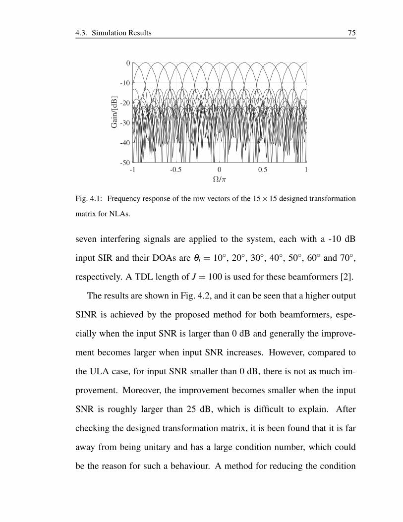
4.3. Simulation Results 75
-1 -0.5 0 0.5 1
/
-50
-40
-30
-20
-10
0
Gai
n/[
dB
]
Fig. 4.1: Frequency response of the row vectors of the 15×15 designed transformation
matrix for NLAs.
seven interfering signals are applied to the system, each with a -10 dB
input SIR and their DOAs are θi = 10, 20, 30, 40, 50, 60 and 70,
respectively. A TDL length of J = 100 is used for these beamformers [2].
The results are shown in Fig. 4.2, and it can be seen that a higher output
SINR is achieved by the proposed method for both beamformers, espe-
cially when the input SNR is larger than 0 dB and generally the improve-
ment becomes larger when input SNR increases. However, compared to
the ULA case, for input SNR smaller than 0 dB, there is not as much im-
provement. Moreover, the improvement becomes smaller when the input
SNR is roughly larger than 25 dB, which is difficult to explain. After
checking the designed transformation matrix, it is been found that it is far
away from being unitary and has a large condition number, which could
be the reason for such a behaviour. A method for reducing the condition
4.4. Fixing Ill Conditioned Transformation Matrix With SVD 76
number even further is introduced in Sec. 4.4 but as mentioned at the end of
Sec. 4.2, further research is needed for designing a unitary transformation
matrix for NLAs with the desired frequency responses.
4.4 Fixing Ill Conditioned Transformation Matrix With
Singular Value Decomposition
It has been mentioned before that, it is important that the transformation
matrix is well conditioned and ideally unitary. A well conditioned matrix
has a low condition number. In section 4.2, the least squares method is
used to design a transformation for NLAs by employing the least squares
filter design method, and then using the diagonal loading method, the con-
dition number of the transformation is reduced. As it was seen in previous
section, an improvement in the performance of the NLAs was achieved but
for low input SNRs the performance was not satisfactory and by analysing
the transformation, it was realised that the condition number of the trans-
formation is still high (around 9). In this section, the singular value decom-
position (SVD) is used to decompose the transformation and subsequently
to modify the transformation to be well-conditioned and as close to unitary
as possible by replacing the low value singular values.
An M ×M transformation matrix A is assumed, which is not unitary.
The SVD of A is
A = UΣVH , (4.8)
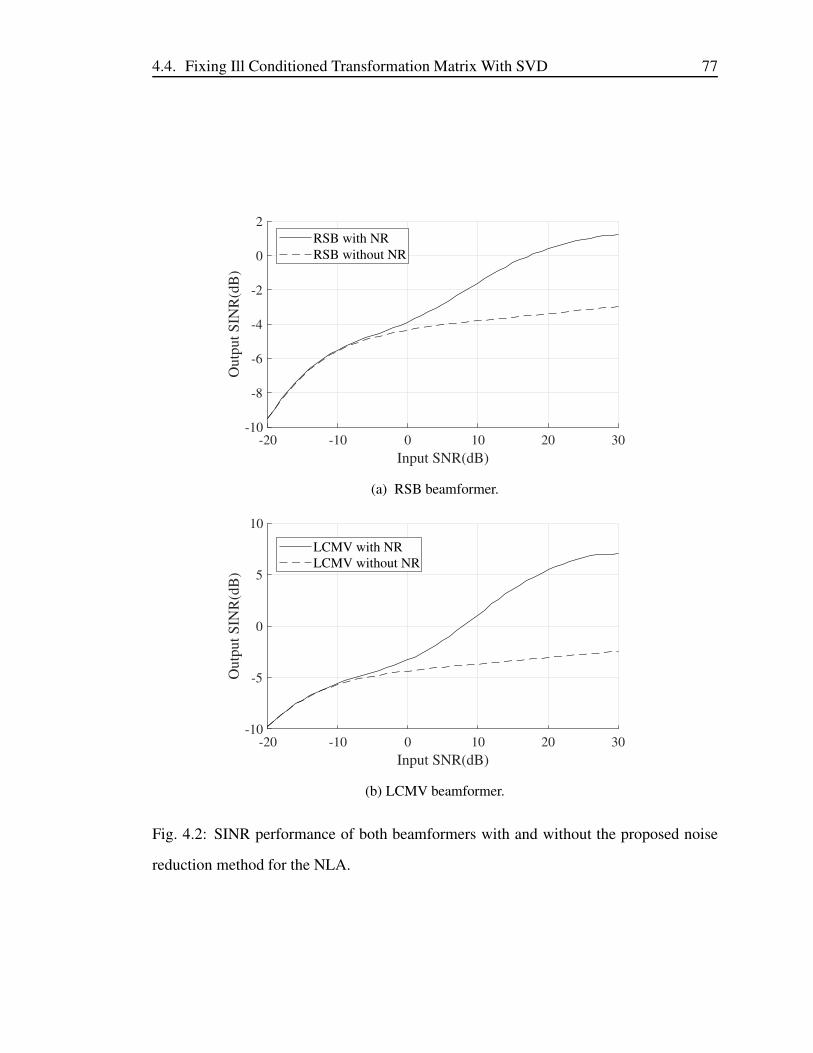
4.4. Fixing Ill Conditioned Transformation Matrix With SVD 77
-20 -10 0 10 20 30
Input SNR(dB)
-10
-8
-6
-4
-2
0
2O
utp
ut
SIN
R(d
B)
RSB with NR
RSB without NR
(a) RSB beamformer.
-20 -10 0 10 20 30
Input SNR(dB)
-10
-5
0
5
10
Ou
tpu
t S
INR
(dB
)
LCMV with NR
LCMV without NR
(b) LCMV beamformer.
Fig. 4.2: SINR performance of both beamformers with and without the proposed noise
reduction method for the NLA.
4.4. Fixing Ill Conditioned Transformation Matrix With SVD 78
where U and V are M×M unitary matrices and Σ is a diagonal rectangular
M×M matrix with singular values σi, i = 0, · · · ,M−1, on the diagonal.
The condition number of a matrix is the largest singular value divided
by the smallest one:
κ =σ0
σM−1. (4.9)
Therefore, small singular values result in a large condition number.
The unitary matrix B which minimises ||A−B||2F is B = UVH , where
||.||F defines the Frobenius norm, and therefore, the closest unitary matrix
to A is B [75,76]. This is actually, equal to replacing all the singular values
with 1, σi = 1, i = 0, · · · ,M−1.
The problem with this method is that, if all singular values are replaced
with 1, the beam-pattern of the row vectors of the transformation may be
changed significantly. Therefore, it is not suitable for transforming the
signal, although the transformation is unitary.
The alternative approach is to replace the singular values smaller than
a threshold value. Using this method, the condition number is reduced but
the singular values which are bigger than the threshold are kept the same.
4.4.1 Simulation
As an example, the NLA case which was mentioned before is considered,
the threshold is set to 0.5, and all the (σi, i = 0, · · · ,M − 1) ≤ 0.5 are re-
placed with 0.5. After replacing the small singular values, the condition
number is reduced to 2.45, which is much better than 9 achieved by the
4.4. Fixing Ill Conditioned Transformation Matrix With SVD 79
diagonal loading previously. In order to analyse the effect on the beam pat-
tern, the side-lobe attenuation and 3 dB beamwidth are calculated before
and after the singular value modification of the transformation. The aver-
age 3 dB beamwidth before the modification is 0.162 in the normalised fre-
quency. The average 3 dB beamwidth after the modification is also 0.162,
and therefore, there is no change in 3 dB beamwidth. Moreover, The aver-
age side-lobe attenuation before the modification is 12.59 dB, and after the
modification is 12.73 dB. So, there is no major change in the beam-pattern
for the transformation, and the proposed modification method works quite
well.
Next, the performance of the noise reduction method is analysed with
the modified transformation with low condition number, when used as a
pre-processing step for TDL beamformers. The NLA array structure has
15 sensors (M = 15) and the desired signal arrives from the broadside
(θd = 0). The transformation is a 15× 15 matrix obtained by the modi-
fied design procedure described. For high-pass filters, 101-tap linear-phase
FIR filters with a common delay of 50 samples are employed. A desired
band-limited wideband signal with a bandwidth of [0.3π ,π ] is received by
the aforementioned NLA from the broadside. Four interfering signals are
applied to the system, each with a -20 dB input SIR and their DOAs are
θi = 10,30,50,70, respectively. A tapped delay line with length J = 5
is used for these beamformers. Fig. 4.3, illustrates the performance of the
two well-known RSB and LCMV beamformers when used with and with-
4.5. Summary 80
out the modified noise reduction method. It is clear that for both RSB and
LCMV beamformers the performance of the beamformer with the modi-
fied noise reduction pre-processing is increased significantly.
4.5 Summary
In this chapter, the noise reduction method introduced in Chapter 3 was
re-designed based on the structure of NLAs. Same as the ULA case, a
maximum of 3 dB improvement in output TSNR was achieved. This TSNR
improvement leads to possible performance enhancement in many array
signal processing applications.
Due to the non-uniform spacing of the NLA, the resultant beam-patterns
of the row vectors are significantly distorted. Therefore, the DFT matrix
is not applicable. The least squares method was used for re-designing the
transformation for NLA. The beam response of DFT matrix was used as
the reference response for the least squares method to design a prototype
filter, and then the prototype was modulated to different subbands to form
the transformation matrix.
Diagonal loading method was used to reduce the condition number of
the designed transformation, and simulation results presented an improve-
ment in output SINR performance for the RSB and LCMV beamformers,
when the noise reduction method is used as a pre-processing step.
Later, the SVD was used to decompose the transformation. By replac-
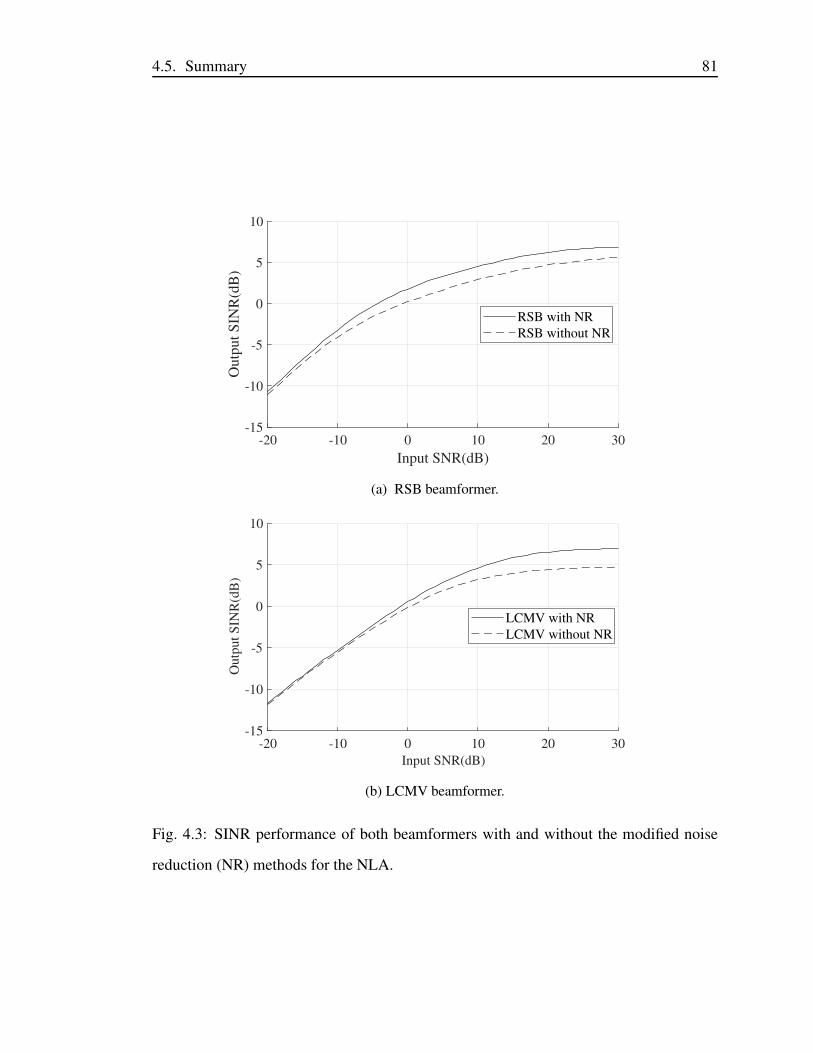
4.5. Summary 81
-20 -10 0 10 20 30
Input SNR(dB)
-15
-10
-5
0
5
10O
utp
ut
SIN
R(d
B)
RSB with NR
RSB without NR
(a) RSB beamformer.
-20 -10 0 10 20 30
Input SNR(dB)
-15
-10
-5
0
5
10
Ou
tpu
t S
INR
(dB
)
LCMV with NR
LCMV without NR
(b) LCMV beamformer.
Fig. 4.3: SINR performance of both beamformers with and without the modified noise
reduction (NR) methods for the NLA.
4.5. Summary 82
ing the low value singular values, the transformation was modified to be
well-conditioned and as close to unitary as possible. The simulation re-
sults showed a steady improvement for RSB and LCMV beamformers for
a wide range of input SNRs from -20 dB to 30dB.
In the following chapter transformation is re-designed for the structure
of planar arrays.
Chapter 5
Extension of the Method to Planar
Arrays
In Chapter 3, a method was developed for reducing the effect of white noise
in wideband ULAs via a combination of a judiciously designed transforma-
tion followed by high-pass filters to improve the performance for wideband
beamforming and DOA estimation. In this chapter, the idea is extended to
the case of planar arrays, and focus on two major types of planar arrays,
namely, uniform rectangular arrays (URAs) [77, 78] and uniform circular
arrays (UCAs) [79, 80]. As a result, the transformation matrix has to be
re-designed to adjust the noise reduction method to the structure of URAs
and UCAs.
In particular, two noise reduction methods are introduced in this chapter
for URAs and for each one, a different transformation is designed. The first
method is based on a two-dimensional (2D) transformation. The second
method is an adaptation of the method introduced in Chapter 3, which
83
5.1. White Noise Reduction for URAs with a 2D Transformation 84
is based on one-dimensional (1D) transformation of the signals received
by the URA. The transformations must be invertible and ideally, unitary.
As representative examples for unitary transformations, 2D-DFT (discrete
Fourier transform) and 1D-DFT are used in simulation.
Later, a method is introduced for the UCAs based on a 1D transforma-
tion. The transformation is re-designed for the UCA structure, by changing
the modulation of the prototype filter to match the structure of the UCA.
All the methods can increase the overall signal-to-noise ratio (SNR) of
the array. This improvement leads to performance enhancement of var-
ious array signal processing applications such as beamforming, which is
demonstrated by simulation using two well-known adaptive beamformers,
namely the RSB [39, 40], and the LCMV beamformers [2, 49].
Part of the contents of this chapter was presented at a conference [81].
5.1 White Noise Reduction for URAs with a 2D Transfor-
mation
The linear arrays are used to resolve the azimuth angle θ of the received
signal, whereas the URA allows to resolve the elevation angle φ in addition
to the azimuth angle θ [82]. Both structures are widely used for developing
different smart antennas.
The structure of a URA is shown in Fig. 5.1, and a block diagram for
the general structure of the proposed noise reduction method is shown in
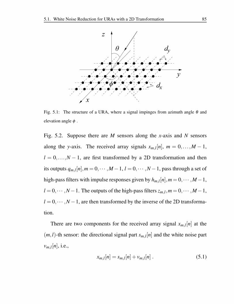
5.1. White Noise Reduction for URAs with a 2D Transformation 85
y
x
y
z
d
d
xϕ
θ
Fig. 5.1: The structure of a URA, where a signal impinges from azimuth angle θ and
elevation angle φ .
Fig. 5.2. Suppose there are M sensors along the x-axis and N sensors
along the y-axis. The received array signals xm,l[n], m = 0, . . . ,M − 1,
l = 0, . . . ,N − 1, are first transformed by a 2D transformation and then
its outputs qm,l[n],m = 0, · · · ,M−1, l = 0, · · · ,N−1, pass through a set of
high-pass filters with impulse responses given by hm,l[n],m = 0, · · · ,M−1,
l = 0, · · · ,N−1. The outputs of the high-pass filters zm,l,m = 0, · · · ,M−1,
l = 0, · · · ,N−1, are then transformed by the inverse of the 2D transforma-
tion.
There are two components for the received array signal xm,l[n] at the
(m, l)-th sensor: the directional signal part sm,l[n] and the white noise part
vm,l[n], i.e.,
xm,l[n] = sm,l[n]+ vm,l[n] . (5.1)
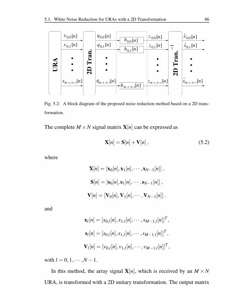
5.1. White Noise Reduction for URAs with a 2D Transformation 86
2D
Tra
n.
n[ ]x 0,0
n[ ]
n[ ]M−1, N−1x
n[ ]
n[ ]
n[ ]M−1, N−1q
n[ ]M−1, N−1h
n[ ]
n[ ]
n[ ]
n[ ]
n[ ]M−1, N−1z
−1
n[ ]x 0,0
n[ ]x0,1
n[ ]M−1, N−1x
0,1x
0,0
0,1
q
q0,0h
0,1h
0,0
0,1
z
z
^
^
^
2D
Tra
n.
UR
A
Fig. 5.2: A block diagram of the proposed noise reduction method based on a 2D trans-
formation.
The complete M×N signal matrix X[n] can be expressed as
X[n] = S[n]+V[n] , (5.2)
where
X[n] = [x0[n],x1[n], · · · ,xN−1[n]] ,
S[n] = [s0[n],s1[n], · · · ,sN−1[n]] ,
V[n] = [V0[n],V1[n], · · · ,VN−1[n]] .
and
xl[n] = [x0,l[n],x1,l[n], · · · ,xM−1,l[n]]T ,
sl[n] = [s0,l[n],s1,l[n], · · · ,sM−1,l[n]]T ,
Vl[n] = [v0,l[n],v1,l[n], · · · ,vM−1,l[n]]T ,
with l = 0,1, · · · ,N −1.
In this method, the array signal X[n], which is received by an M ×N
URA, is transformed with a 2D unitary transformation. The output matrix
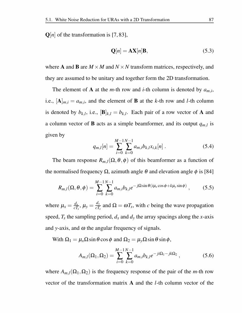
5.1. White Noise Reduction for URAs with a 2D Transformation 87
Q[n] of the transformation is [7, 83],
Q[n] = AX[n]B, (5.3)
where A and B are M×M and N×N transform matrices, respectively, and
they are assumed to be unitary and together form the 2D transformation.
The element of A at the m-th row and i-th column is denoted by am,i,
i.e., [A]m,i = am,i, and the element of B at the k-th row and l-th column
is denoted by bk,l, i.e., [B]k,l = bk,l. Each pair of a row vector of A and
a column vector of B acts as a simple beamformer, and its output qm,l is
given by
qm,l[n] =M−1
∑i=0
N−1
∑k=0
am,ibk,lxi,k[n] . (5.4)
The beam response Rm,l(Ω,θ ,φ) of this beamformer as a function of
the normalised frequency Ω, azimuth angle θ and elevation angle φ is [84]
Rm,l(Ω,θ ,φ) =M−1
∑i=0
N−1
∑k=0
am,ibk,le− jΩsinθ(iµx cosφ+kµy sinφ) , (5.5)
where µx =dx
cTs, µy =
dy
cTsand Ω = ωTs, with c being the wave propagation
speed, Ts the sampling period, dx and dy the array spacings along the x-axis
and y-axis, and ω the angular frequency of signals.
With Ω1 = µxΩsinθ cosφ and Ω2 = µyΩsinθ sinφ ,
Am,l(Ω1,Ω2) =M−1
∑i=0
N−1
∑k=0
am,ibk,le− jiΩ1− jkΩ2 , (5.6)
where Am,l(Ω1,Ω2) is the frequency response of the pair of the m-th row
vector of the transformation matrix A and the l-th column vector of the
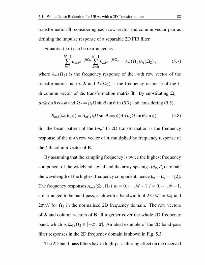
5.1. White Noise Reduction for URAs with a 2D Transformation 88
transformation B, considering each row vector and column vector pair as
defining the impulse response of a separable 2D FIR filter.
Equation (5.6) can be rearranged as
M−1
∑i=0
am,ie− jiΩ1
N−1
∑k=0
bk,le− jkΩ2 = Am(Ω1)Al(Ω2) , (5.7)
where Am(Ω1) is the frequency response of the m-th row vector of the
transformation matrix A and Al(Ω2) is the frequency response of the l-
th column vector of the transformation matrix B. By substituting Ω1 =
µxΩsinθ cosφ and Ω2 = µyΩsinθ sinφ in (5.7) and considering (5.5),
Rm,l(Ω,θ ,φ) = Am(µxΩsinθ cosφ)Al(µyΩsinθ sinφ) . (5.8)
So, the beam pattern of the (m,l)-th 2D transformation is the frequency
response of the m-th row vector of A multiplied by frequency response of
the l-th column vector of B.
By assuming that the sampling frequency is twice the highest frequency
component of the wideband signal and the array spacings (dx, dy) are half
the wavelength of the highest frequency component, hence µx = µy = 1 [2].
The frequency responses Am,l(Ω1,Ω2),m = 0, · · · ,M−1, l = 0, · · · ,N −1,
are arranged to be band-pass, each with a bandwidth of 2π/M for Ω1 and
2π/N for Ω2 in the normalised 2D frequency domain. The row vectors
of A and column vectors of B all together cover the whole 2D frequency
band, which is Ω1,Ω2 ∈ [−π : π ]. An ideal example of the 2D band-pass
filter responses in the 2D frequency domain is shown in Fig. 5.3.
The 2D band-pass filters have a high-pass filtering effect on the received
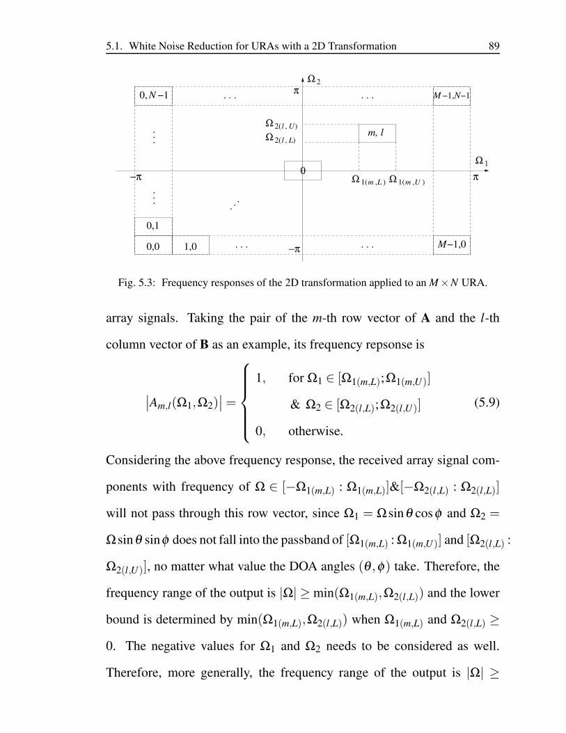
5.1. White Noise Reduction for URAs with a 2D Transformation 89
0
0, −1
−1,0M
Lm1( , )Ω Ω m U1( , )
. . .
. . .
. . .
0,0 . . . . . .1,0
. . .
Ω
Ω
2
1
Ω
Ω
−π
π
−π π
. . . M N−1, −1
L
l
l2( , )
2( , )Um, l
0,1
N
Fig. 5.3: Frequency responses of the 2D transformation applied to an M×N URA.
array signals. Taking the pair of the m-th row vector of A and the l-th
column vector of B as an example, its frequency repsonse is
∣
∣Am,l(Ω1,Ω2)∣
∣=
1, for Ω1 ∈ [Ω1(m,L);Ω1(m,U)]
& Ω2 ∈ [Ω2(l,L);Ω2(l,U)]
0, otherwise.
(5.9)
Considering the above frequency response, the received array signal com-
ponents with frequency of Ω ∈ [−Ω1(m,L) : Ω1(m,L)]&[−Ω2(l,L) : Ω2(l,L)]
will not pass through this row vector, since Ω1 = Ωsinθ cosφ and Ω2 =
Ωsinθ sinφ does not fall into the passband of [Ω1(m,L) : Ω1(m,U)] and [Ω2(l,L) :
Ω2(l,U)], no matter what value the DOA angles (θ ,φ) take. Therefore, the
frequency range of the output is |Ω| ≥ min(Ω1(m,L),Ω2(l,L)) and the lower
bound is determined by min(Ω1(m,L),Ω2(l,L)) when Ω1(m,L) and Ω2(l,L) ≥
0. The negative values for Ω1 and Ω2 needs to be considered as well.
Therefore, more generally, the frequency range of the output is |Ω| ≥
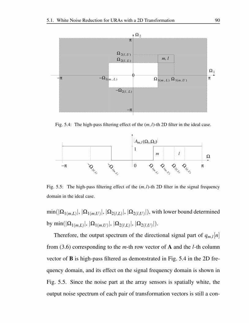
5.1. White Noise Reduction for URAs with a 2D Transformation 90
1( , )
Ω
Ω
2
1
−π
π
−π πm L−Ω1( , ) Ω
Ω
Ω
−Ω
l
l
l
U
L
2( , )
2( , )
L2( , )
m, l
Ω0
m U1( , )m L
Fig. 5.4: The high-pass filtering effect of the (m, l)-th 2D filter in the ideal case.
1( , )
m L
−π π0
Ω
1
−Ω2( , )
ΩΩ2( , )
l U2( , )
l L
l
A
l L
(Ω ,Ω )1 2m,l
−Ω Ω m
L
1( , )
m
Ω m
U
1( , )
Fig. 5.5: The high-pass filtering effect of the (m, l)-th 2D filter in the signal frequency
domain in the ideal case.
min(|Ω1(m,L)|, |Ω1(m,U)|, |Ω2(l,L)|, |Ω2(l,U)|), with lower bound determined
by min(|Ω1(m,L)|, |Ω1(m,U)|, |Ω2(l,L)|, |Ω2(l,U)|).
Therefore, the output spectrum of the directional signal part of qm,l[n]
from (3.6) corresponding to the m-th row vector of A and the l-th column
vector of B is high-pass filtered as demonstrated in Fig. 5.4 in the 2D fre-
quency domain, and its effect on the signal frequency domain is shown in
Fig. 5.5. Since the noise part at the array sensors is spatially white, the
output noise spectrum of each pair of transformation vectors is still a con-
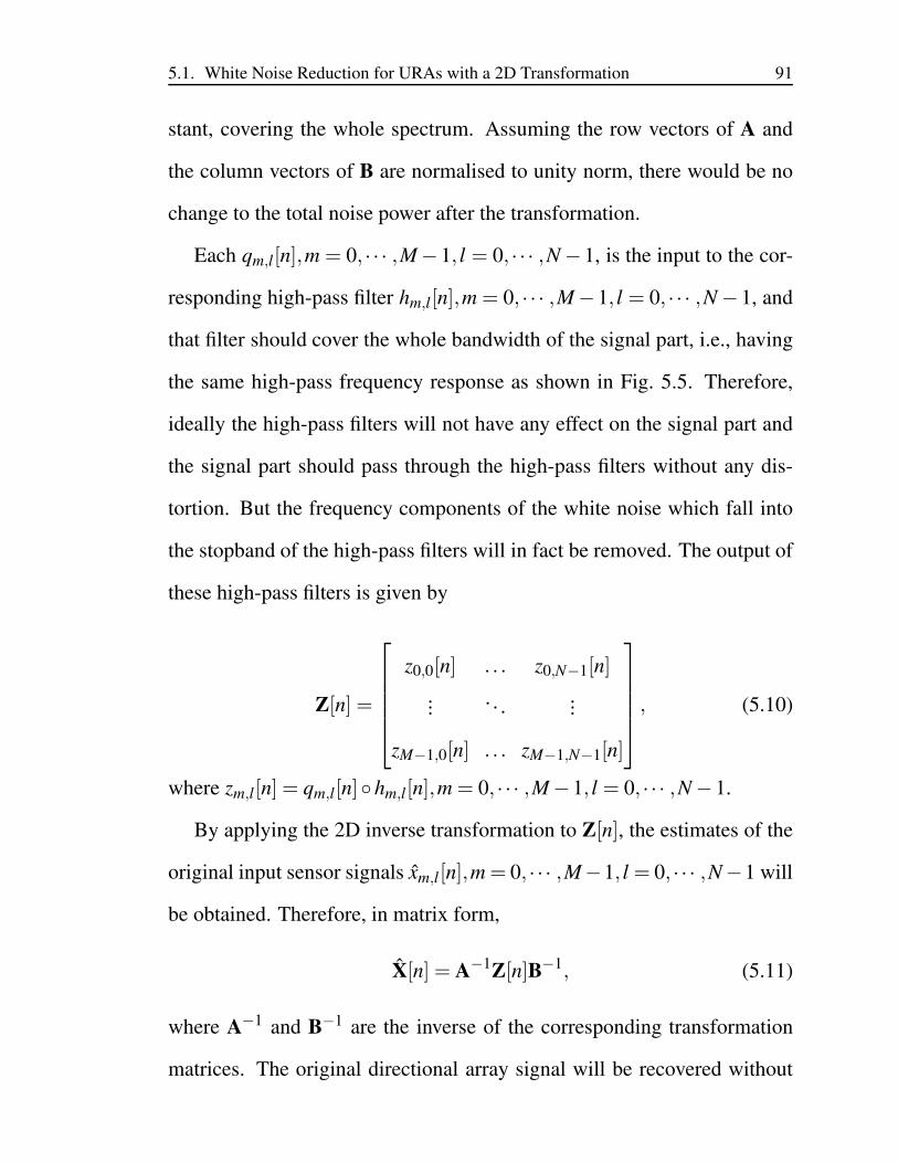
5.1. White Noise Reduction for URAs with a 2D Transformation 91
stant, covering the whole spectrum. Assuming the row vectors of A and
the column vectors of B are normalised to unity norm, there would be no
change to the total noise power after the transformation.
Each qm,l[n],m = 0, · · · ,M−1, l = 0, · · · ,N −1, is the input to the cor-
responding high-pass filter hm,l[n],m = 0, · · · ,M−1, l = 0, · · · ,N −1, and
that filter should cover the whole bandwidth of the signal part, i.e., having
the same high-pass frequency response as shown in Fig. 5.5. Therefore,
ideally the high-pass filters will not have any effect on the signal part and
the signal part should pass through the high-pass filters without any dis-
tortion. But the frequency components of the white noise which fall into
the stopband of the high-pass filters will in fact be removed. The output of
these high-pass filters is given by
Z[n] =
z0,0[n] . . . z0,N−1[n]
.... . .
...
zM−1,0[n] . . . zM−1,N−1[n]
, (5.10)
where zm,l[n] = qm,l[n]hm,l[n],m = 0, · · · ,M−1, l = 0, · · · ,N −1.
By applying the 2D inverse transformation to Z[n], the estimates of the
original input sensor signals xm,l[n],m = 0, · · · ,M−1, l = 0, · · · ,N−1 will
be obtained. Therefore, in matrix form,
X[n] = A−1Z[n]B−1, (5.11)
where A−1 and B−1 are the inverse of the corresponding transformation
matrices. The original directional array signal will be recovered without
5.2. White Noise Reduction for URAs with a 1D Transformation 92
distortion in the ideal case, while the noise power will be reduced, leading
to an improved TSNR.
Considering the stopband of each high-pass filter, the total effect of the
high-pass filters on the total noise power can be calculated. By using nu-
meric methods, it has been calculated that when M, N → ∞, the power of
noise will be reduced by 1.76 dB. Therefore, up to a maximum of 1.76 dB
improvement in TSNR can be achieved. However, in practice, the TSNR
improvement will be less than that, due to the limited number of sensors
in the URA. This TSNR improvement is less than the 3 dB improvement
which was achieved for ULAs using a 1D unitary transformation as in
Chapter 3. In the next section, as an alternative approach, the noise re-
duction method for ULAs is adapted to be applicable to URAs, in order to
achieve a higher output TSNR.
5.2 White Noise Reduction for URAs with a 1D Transfor-
mation
In this approach, the method developed for ULAs in Chapter 3 is adapted
for the URA structure. Each column of the sensors of a URA is actually
a ULA. Therefore, each column of the sensors is taken separately as a
ULA and the previously developed noise reduction method is applied for
the ULAs to each column. As a result, along each column of sensors a 3
dB improvement in the SNR of that column is achieved. Considering the
5.2. White Noise Reduction for URAs with a 1D Transformation 93
whole URA structure, the TSNR is improved by 3 dB. In the following,
this approach is explained in more details.
Assume the l-th column of sensors along the x-axis, is considered for
processing. xl[n]=[x0,l [n], x1,l[n], · · · , xM−1,l[n]]T is the signal vector ac-
cording to this column. xl[n] is transformed with a 1D transformation ma-
trix such as A, with size M×M. After transforming xl[n], the output signal
vector ql[n] is obtained as
ql[n] = Axl[n], (5.12)
where ql[n] = [q0,l[n], · · · ,qM−1,l[n]]T .
The high-pass filtering effect of the transformation for ULAs has been
shown in Chapter 3. Because of the high-pass filtering effect of the trans-
formation on the directional signal, the output spectrum of the directional
signal part of qm,l[n] corresponding to the m-th row vector of A is high-
pass filtered. As the noise part of the array sensors is spatially white, the
output noise spectrum of the row vector is still a constant, covering the
whole spectrum. Since A is assumed to be unitary and the row vectors of
A are normalised to unity norm, therefore, there would be no change to the
total noise power after transformation.
Similar to the explanation for (5.10), each qm,l[n],m = 0, · · · ,M − 1, is
the input to the corresponding high-pass filter hm,l[n],m = 0, · · · ,M − 1,
and the high-pass filter should cover the whole bandwidth of the signal
part, i.e., having the same high-pass frequency response. Therefore, ide-
5.2. White Noise Reduction for URAs with a 1D Transformation 94
ally the high-pass filters will not have any effect on the signal part and
the signal part should pass through the high-pass filters without any distor-
tion. However, frequency components of the white noise which fall into
the stopband of the high-pass filters will be removed. The output of these
high-pass filters is given by
zl[n] =
z0,l[n]
z1,l[n]
...
zM−1,l[n]
=
q0,l[n]h0,l[n]
q1,l[n]h1,l[n]
...
qM−1,l[n]hM−1,l[n]
. (5.13)
By applying the inverse of the transformation matrix (A−1) to zl[n], the
estimates of the original input sensor signals xm,l[n], m = 0, · · · ,M − 1 is
obtained. Therefore, in vector form,
xl[n] = A−1zl[n], (5.14)
where xl[n] = [x0,l[n], x1,l[n], · · · , xM−1,l[n]]T . After going through these
processing stages, ideally, there is no change in the signal part in the final
output xm,l[n], m = 0, · · · ,M − 1, compared to the original signal part in
xm,l[n], m = 0, · · · ,M − 1. However, since A−1 is also unitary, the total
noise power stays the same between xl[n] and zl[n]. Following the same
analysis for the ULA case as discussed in Chapter 3, the same conclusion
can be drawn that up to 3 dB TSNR improvement can be obtained by the
proposed method. However, in practice, the SNR improvement will be less
than 3 dB due to the limited number of sensors. The same process needs to
5.3. White Noise Reduction for UCAs 95
be applied to all the columns of sensors of the URA across the x-axis, and
for each column of sensors a 3 dB improvement in TSNR will be achieved.
However, one important point is that, although the TSNR improvement
is 3 dB and much higher than the case of the 2D transformation devel-
oped in the last section, the side-lobe attenuation of the 1D case will be
much less than the 2D case. Because as shown in (5.8), the beam-pattern
of the 2D transformation is the multiplication of the beam-patterns of its
corresponding row/column vectors. A direct consequence will be more
distortion to the signal part using the 1D transformation when discarding
the noise components using the high-pass filters. As a result, the perfor-
mance improvement may be less than the method directly based on the 2D
transformation. This will be demonstrated in simulation section.
5.3 White Noise Reduction for UCAs
In this section, the method is extended to uniform circular arrays (UCAs)
which is another type of planar arrays. Therefore, the transformation is
re-designed to adjust the noise reduction method to the structure of UCAs.
The method introduced in this section is based on a 1D transforma-
tion and is an adaptation of the method introduced in Chapter 3. Same as
before, the transformation should be invertible and ideally, unitary. The
circular arrays have a sparse structure naturally. Therefore, designing an
ideal unitary transformation is not always possible. First, the transforma-
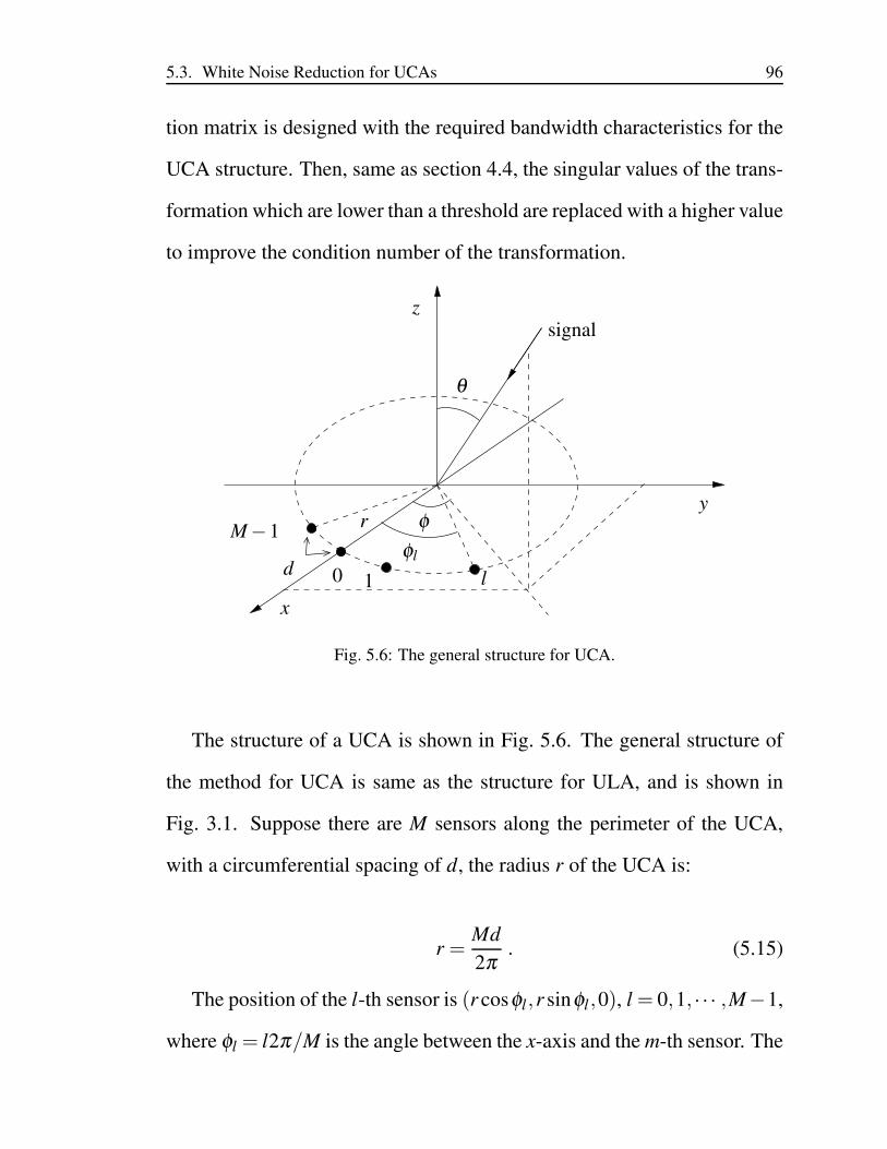
5.3. White Noise Reduction for UCAs 96
tion matrix is designed with the required bandwidth characteristics for the
UCA structure. Then, same as section 4.4, the singular values of the trans-
formation which are lower than a threshold are replaced with a higher value
to improve the condition number of the transformation.
x
y
z
d
signal
θ
φ
φl
M−1
0 1 l
r
Fig. 5.6: The general structure for UCA.
The structure of a UCA is shown in Fig. 5.6. The general structure of
the method for UCA is same as the structure for ULA, and is shown in
Fig. 3.1. Suppose there are M sensors along the perimeter of the UCA,
with a circumferential spacing of d, the radius r of the UCA is:
r =Md
2π. (5.15)
The position of the l-th sensor is (r cosφl,r sinφl,0), l = 0,1, · · · ,M−1,
where φl = l2π/M is the angle between the x-axis and the m-th sensor. The
5.3. White Noise Reduction for UCAs 97
spacing d is α/2 times the wavelength of the highest frequency component
of the signal λmin, and therefore, d = αλmin/2, where α is a scalar value.
So, r is [85, 86]:
r = αλmin
2
M
2π. (5.16)
Considering β = M/2π ,
r = αβλmin
2. (5.17)
The phase difference between the centre of the UCA and the l-th sensor is:
Φ = ωr sinθ cos(φ −φl)
c, (5.18)
where ω is the angular frequency of the signal and c is the wave propaga-
tion speed. By plugging (5.16) into (5.18),
Φ =ωλmin
2cαβ sinθ cos(φ −φl) . (5.19)
Ω = ωTs by considering the sampling frequency of Ts = λmin/2c. There-
fore, the l-th element of d(Ω,θ ,φ) which is the steering vector of the UCA
is [79, 87]:
dl = e jαβΩsin θ cos(φ−φl) . (5.20)
The transformation can be designed for the UCA using the steering vec-
tor. The row vectors of the transformation matrix are each a band-pass filter
and together they cover the entire normalised frequency range of the sig-
nal. Same as before, first a low-pass filter with the required characteristics
is designed as the prototype filter. Then, the prototype filter is modulated
to each subband of the transformation. Considering p is the prototype
5.3. White Noise Reduction for UCAs 98
filter with length M, p can be modulated to cover the entire normalised
frequency band, using
am,l = e− jαβ 2πM
mcos(φ−φl)pl , (5.21)
where m = 0, · · · ,M−1, l = 0, · · · ,M−1. Note that, for different elevation
angles φ , the transformation changes, and the design gives different results.
Therefore, the elevation angle φ of the desired signal should be known to
design the transformation. For the signals not coming from φ used for
the design, the frequency response of the transformation is different, so in
here, it is assumed that the impinging signals are coming from the same φ .
If the elevation angle φ of the desired signal changes, the transformation
should be re-designed, or alternatively, pre-steering can be used to adjust
the impinging signal to the transformation.
In this work, it is assumed that φ = π/2. Therefore, (5.21) can be
written as:
am,l = e− jαβ 2πM
mcos(π2−φl)pl . (5.22)
The beam response Rm(Ω,θ) of a row vector of the transformation is:
Rm(Ω,θ) =M−1
∑l=0
am,lejαβΩsinθ cos(π
2−φl) . (5.23)
With Ω = Ωsinθ , Rm(Ω,θ) can be represented in the following form:
Am(Ω) =M−1
∑l=0
am,lejαβ Ωcos(π
2−φl), (5.24)
where Am(Ω) is the frequency response of the m-th row vector of the trans-
formation.
5.4. Simulation Results 99
The frequency responses are designed to be band-pass, each with a
bandwidth of 2π/M, and altogether they cover the entire normalised fre-
quency band. The band-pass filters have high-pass filtering effect on the
received signals with φ = π/2, and different values for θ . The examina-
tion of the high-pass behaviour is same as the examination provided for the
ULA case in Sec. 3.1.
The transformation should be invertible and ideally unitary. The cir-
cular arrays are sparse in general [88]. Therefore, if the transformation
matrix is ill-conditioned, the approach introduced in Sec. 4.4 can be used
to reduce the condition number of the transformation, without causing a
significant change in the beam pattern of the transformation.
After designing a well-conditioned transformation with the required fre-
quency responses, the high-pass filters are applied and then the signal is
transformed back, similar to the block diagram illustrated in Fig. 3.1.
5.4 Simulation Results
In this section, simulation results will be provided and compared to verify
the effectiveness of the proposed noise reduction pre-processing methods
for the URA and UCA structures.
5.4. Simulation Results 100
5.4.1 Simulation for the URA structure
For simplicity, the same number of sensors is used across the x-axis and
y-axis (M = N), with the same array spacings (dx = dy). The URA has 16
sensors along each axis (M = 16) and the desired signal arrives from the
broadside (θd,φd = 0). The transformation matrix A = B is a 16×16 DFT
matrix, as an example of unitary transformation. For the high-pass filters,
linear phase 101-tap FIR filters with a common delay of 50 samples are
employed. Then, the array signals are transformed back by the inverse of
the transformation matrix (A−1).
As mentioned before, by using the 2D transformation method, up to
1.76 dB and by using the 1D transformation method, up to 3 dB TSNR
improvement can be achieved. Despite lower TSNR improvement, the 2D
transformation method has less distortion on the directional signal, because
the 2D transformation vectors have a higher side-lobe attenuation, due to
the dual filtering process along both axes. Frequency responses of an ex-
ample 2D-DFT vector in the frequency domain and its corresponding 1D-
DFT vector, for the directional signal arriving from θ = 90 and φ = 45
are shown in Fig. 5.7. It can be clearly seen that the side-lobe attenuation
for the 2D-DFT is around 26 dB, whereas the side-lobe attenuation for the
1D-DFT is around 13 dB. This results to less amount of directional sig-
nals available in the lower side-lobes of the 2D-DFT, to be removed by the
high-pass filters compared to the 1D-DFT. Therefore, a better recovery for
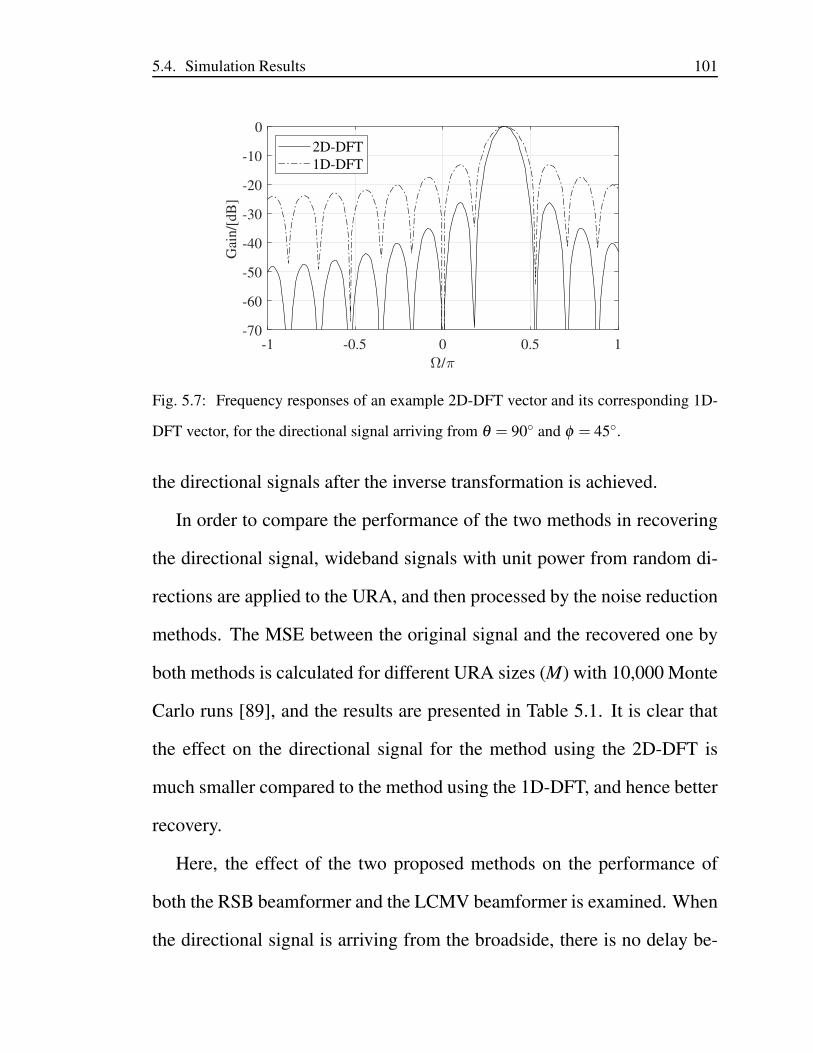
5.4. Simulation Results 101
-1 -0.5 0 0.5 1
/
-70
-60
-50
-40
-30
-20
-10
0
Gai
n/[
dB
]
2D-DFT
1D-DFT
Fig. 5.7: Frequency responses of an example 2D-DFT vector and its corresponding 1D-
DFT vector, for the directional signal arriving from θ = 90 and φ = 45.
the directional signals after the inverse transformation is achieved.
In order to compare the performance of the two methods in recovering
the directional signal, wideband signals with unit power from random di-
rections are applied to the URA, and then processed by the noise reduction
methods. The MSE between the original signal and the recovered one by
both methods is calculated for different URA sizes (M) with 10,000 Monte
Carlo runs [89], and the results are presented in Table 5.1. It is clear that
the effect on the directional signal for the method using the 2D-DFT is
much smaller compared to the method using the 1D-DFT, and hence better
recovery.
Here, the effect of the two proposed methods on the performance of
both the RSB beamformer and the LCMV beamformer is examined. When
the directional signal is arriving from the broadside, there is no delay be-
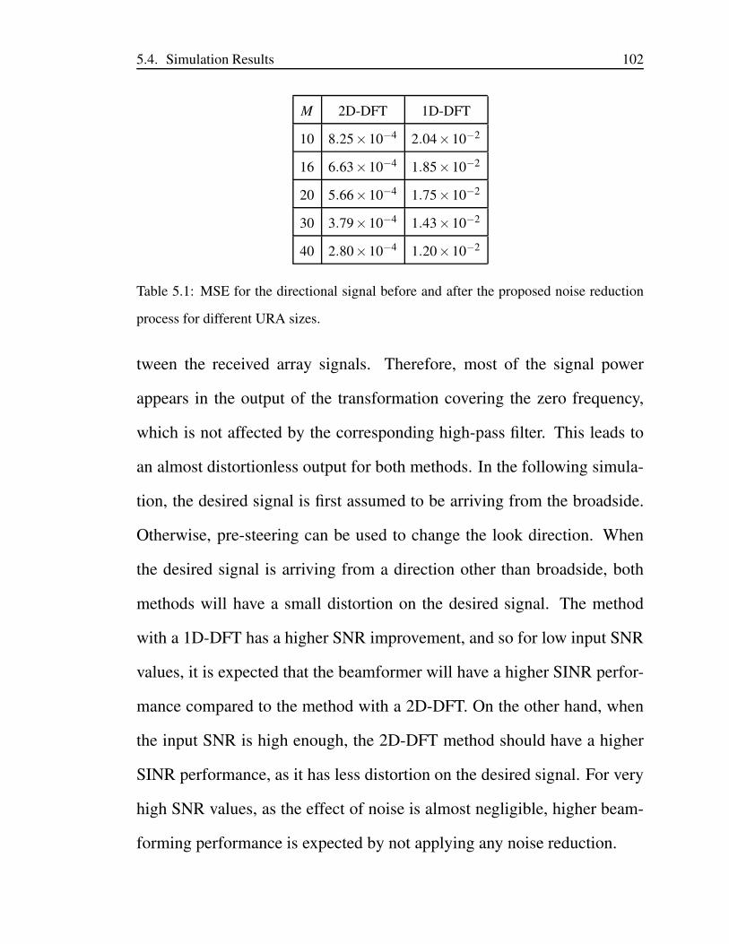
5.4. Simulation Results 102
M 2D-DFT 1D-DFT
10 8.25×10⁻⁴ 2.04×10⁻²
16 6.63×10⁻⁴ 1.85×10⁻²
20 5.66×10⁻⁴ 1.75×10⁻²
30 3.79×10⁻⁴ 1.43×10⁻²
40 2.80×10⁻⁴ 1.20×10⁻²
Table 5.1: MSE for the directional signal before and after the proposed noise reduction
process for different URA sizes.
tween the received array signals. Therefore, most of the signal power
appears in the output of the transformation covering the zero frequency,
which is not affected by the corresponding high-pass filter. This leads to
an almost distortionless output for both methods. In the following simula-
tion, the desired signal is first assumed to be arriving from the broadside.
Otherwise, pre-steering can be used to change the look direction. When
the desired signal is arriving from a direction other than broadside, both
methods will have a small distortion on the desired signal. The method
with a 1D-DFT has a higher SNR improvement, and so for low input SNR
values, it is expected that the beamformer will have a higher SINR perfor-
mance compared to the method with a 2D-DFT. On the other hand, when
the input SNR is high enough, the 2D-DFT method should have a higher
SINR performance, as it has less distortion on the desired signal. For very
high SNR values, as the effect of noise is almost negligible, higher beam-
forming performance is expected by not applying any noise reduction.
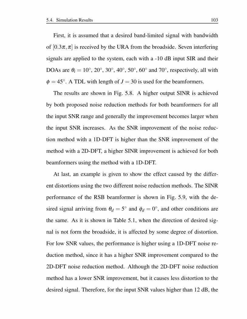
5.4. Simulation Results 103
First, it is assumed that a desired band-limited signal with bandwidth
of [0.3π ,π ] is received by the URA from the broadside. Seven interfering
signals are applied to the system, each with a -10 dB input SIR and their
DOAs are θi = 10, 20, 30, 40, 50, 60 and 70, respectively, all with
φ = 45. A TDL with length of J = 30 is used for the beamformers.
The results are shown in Fig. 5.8. A higher output SINR is achieved
by both proposed noise reduction methods for both beamformers for all
the input SNR range and generally the improvement becomes larger when
the input SNR increases. As the SNR improvement of the noise reduc-
tion method with a 1D-DFT is higher than the SNR improvement of the
method with a 2D-DFT, a higher SINR improvement is achieved for both
beamformers using the method with a 1D-DFT.
At last, an example is given to show the effect caused by the differ-
ent distortions using the two different noise reduction methods. The SINR
performance of the RSB beamformer is shown in Fig. 5.9, with the de-
sired signal arriving from θd = 5 and φd = 0, and other conditions are
the same. As it is shown in Table 5.1, when the direction of desired sig-
nal is not form the broadside, it is affected by some degree of distortion.
For low SNR values, the performance is higher using a 1D-DFT noise re-
duction method, since it has a higher SNR improvement compared to the
2D-DFT noise reduction method. Although the 2D-DFT noise reduction
method has a lower SNR improvement, but it causes less distortion to the
desired signal. Therefore, for the input SNR values higher than 12 dB, the
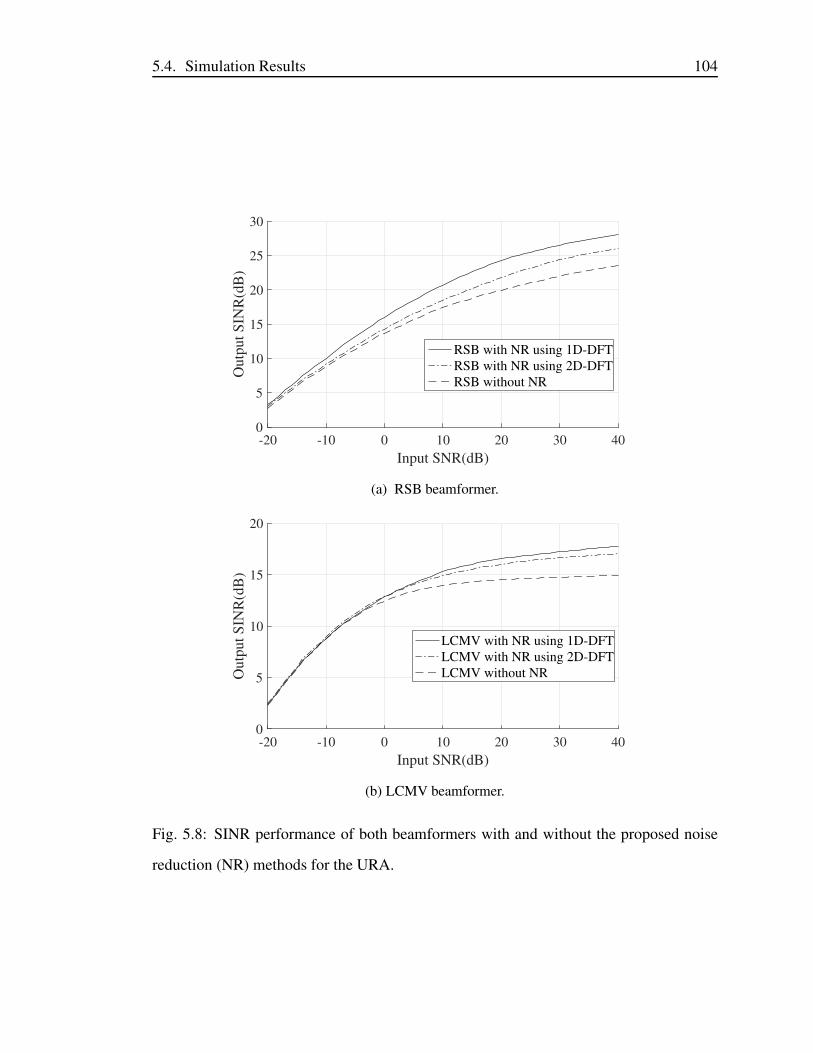
5.4. Simulation Results 104
-20 -10 0 10 20 30 40
Input SNR(dB)
0
5
10
15
20
25
30
Ou
tpu
t S
INR
(dB
)
RSB with NR using 1D-DFT
RSB with NR using 2D-DFT
RSB without NR
(a) RSB beamformer.
-20 -10 0 10 20 30 40
Input SNR(dB)
0
5
10
15
20
Ou
tpu
t S
INR
(dB
)
LCMV with NR using 1D-DFT
LCMV with NR using 2D-DFT
LCMV without NR
(b) LCMV beamformer.
Fig. 5.8: SINR performance of both beamformers with and without the proposed noise
reduction (NR) methods for the URA.
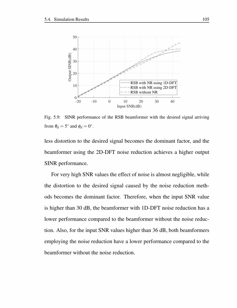
5.4. Simulation Results 105
-20 -10 0 10 20 30 40
Input SNR(dB)
0
10
20
30
40
50
Ou
tpu
t S
INR
(dB
)
RSB with NR using 1D-DFT
RSB with NR using 2D-DFT
RSB without NR
Fig. 5.9: SINR performance of the RSB beamformer with the desired signal arriving
from θd = 5 and φd = 0.
less distortion to the desired signal becomes the dominant factor, and the
beamformer using the 2D-DFT noise reduction achieves a higher output
SINR performance.
For very high SNR values the effect of noise is almost negligible, while
the distortion to the desired signal caused by the noise reduction meth-
ods becomes the dominant factor. Therefore, when the input SNR value
is higher than 30 dB, the beamformer with 1D-DFT noise reduction has a
lower performance compared to the beamformer without the noise reduc-
tion. Also, for the input SNR values higher than 36 dB, both beamformers
employing the noise reduction have a lower performance compared to the
beamformer without the noise reduction.
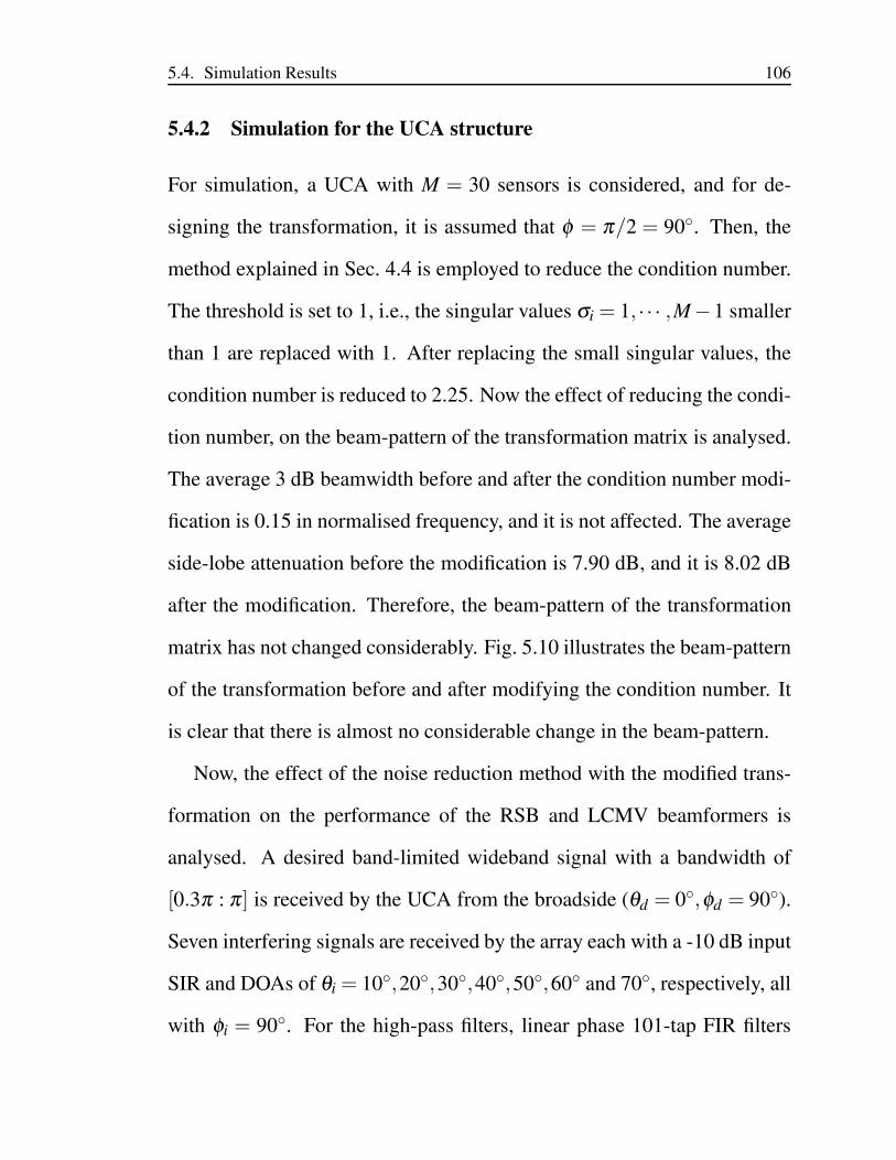
5.4. Simulation Results 106
5.4.2 Simulation for the UCA structure
For simulation, a UCA with M = 30 sensors is considered, and for de-
signing the transformation, it is assumed that φ = π/2 = 90. Then, the
method explained in Sec. 4.4 is employed to reduce the condition number.
The threshold is set to 1, i.e., the singular values σi = 1, · · · ,M−1 smaller
than 1 are replaced with 1. After replacing the small singular values, the
condition number is reduced to 2.25. Now the effect of reducing the condi-
tion number, on the beam-pattern of the transformation matrix is analysed.
The average 3 dB beamwidth before and after the condition number modi-
fication is 0.15 in normalised frequency, and it is not affected. The average
side-lobe attenuation before the modification is 7.90 dB, and it is 8.02 dB
after the modification. Therefore, the beam-pattern of the transformation
matrix has not changed considerably. Fig. 5.10 illustrates the beam-pattern
of the transformation before and after modifying the condition number. It
is clear that there is almost no considerable change in the beam-pattern.
Now, the effect of the noise reduction method with the modified trans-
formation on the performance of the RSB and LCMV beamformers is
analysed. A desired band-limited wideband signal with a bandwidth of
[0.3π : π ] is received by the UCA from the broadside (θd = 0,φd = 90).
Seven interfering signals are received by the array each with a -10 dB input
SIR and DOAs of θi = 10,20,30,40,50,60 and 70, respectively, all
with φi = 90. For the high-pass filters, linear phase 101-tap FIR filters
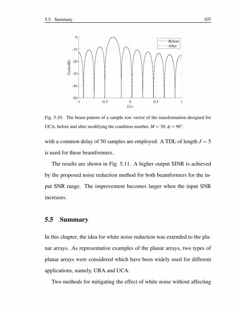
5.5. Summary 107
-1 -0.5 0 0.5 1
/
-50
-40
-30
-20
-10
0
Gai
n(d
B)
Before
After
Fig. 5.10: The beam-pattern of a sample row vector of the transformation designed for
UCA, before and after modifying the condition number, M = 30, φ = 90.
with a common delay of 50 samples are employed. A TDL of length J = 5
is used for these beamformers.
The results are shown in Fig. 5.11. A higher output SINR is achieved
by the proposed noise reduction method for both beamformers for the in-
put SNR range. The improvement becomes larger when the input SNR
increases.
5.5 Summary
In this chapter, the idea for white noise reduction was extended to the pla-
nar arrays. As representative examples of the planar arrays, two types of
planar arrays were considered which have been widely used for different
applications, namely, URA and UCA.
Two methods for mitigating the effect of white noise without affecting
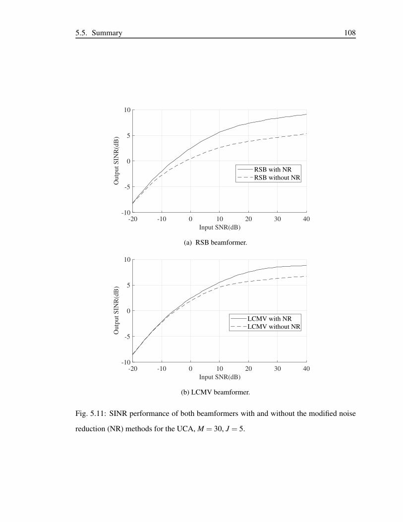
5.5. Summary 108
-20 -10 0 10 20 30 40
Input SNR(dB)
-10
-5
0
5
10O
utp
ut
SIN
R(d
B)
RSB with NR
RSB without NR
(a) RSB beamformer.
-20 -10 0 10 20 30 40
Input SNR(dB)
-10
-5
0
5
10
Ou
tpu
t S
INR
(dB
)
LCMV with NR
LCMV without NR
(b) LCMV beamformer.
Fig. 5.11: SINR performance of both beamformers with and without the modified noise
reduction (NR) methods for the UCA, M = 30, J = 5.
5.5. Summary 109
the directional signal in wideband URAs have been introduced. With the
proposed method using a 2D transformation, a maximum of 1.76 dB im-
provement in TSNR can be achieved in the ideal case, which is less than
the 3 dB improvement previously achieved for ULAs. As an alternative,
the noise reduction method using a 1D transformation for the URAs was
proposed, which is a direct adaptation of the method used for ULAs, with
a 3 dB improvement achieved. Despite lower improvement in TSNR, the
2D transformation method has less distortion for directional signals.
Later, a method based on 1D transformation was introduced for the
UCAs, with a maximum of 3 dB improvement in TSNR. Due to the sparse
nature of the UCA structure, the transformation is not unitary, and the con-
dition number of the transformation is high. Therefore, same as Chapter 4,
the transformation was modified by replacing the low value singular values
of the transformation.
The increased TSNR can be translated into performance improvement
in various planar array signal processing applications and as an example its
effect on adaptive beamforming was studied. As demonstrated by simula-
tion results, a clear improvement in performance in terms of output SINR
has been achieved for a range of input SNR values.
Chapter 6
Further Insights into the Proposed
Noise Reduction Method
As it can be seen from the proposed structure in Chapter. 3, no prior in-
formation is needed about the impinging signals to reduce the noise level
and increase the overall SNR by about 3 dB. However, although the SNR
has been improved, the noise is not white any more, as specified in (3.34),
whose effect on the ultimate performance of the system can not be seen
directly. That is why both theoretical analyses and computer simulation
are provided to show that indeed by the proposed method, the performance
of the two studied beamformers has been improved.
The result in the previous chapters is obtained from the viewpoint of
reducing the noise level of the received signals. In this chapter, the benefits
of the method is discussed from a broader point of view.
The contents of this chapter is published in [50].
110
6.1. The TDL Equivalent Structure 111
6.1 The TDL Equivalent Structure
Actually by studying the structure further, it is realised that the proposed
structure is equivalent to a traditional TDL system, but with a much larger
TDL length. As a result, by applying the same LCMV beamformer (with
the same TDL length) to both the original set of array signals and the
new set of array signals after the proposed pre-processing, the latter one
will be equivalent to a kind of LCMV beamformer but with much longer
TDLs, and hence the improved performance. From this viewpoint, the
proposed method can also be considered as a low-complexity approach to
adaptive beamforming. Certainly another advantage is that the proposed
pre-processing is standard and can be applied to the original array signals,
whatever the following processing (either beamforming or DOA estima-
tion, or tracking, etc.) is. As shown in the study for DOA estimation based
on the proposed structure in [51], the improved SNR can be translated into
improved DOA estimation performance too.
To show that the overall combination of the proposed noise reduction
part and the following TDL-based beamformer is equivalent to a new beam-
former with a much longer TDL, i.e., the noise reduction method along-
side the TDL attached can be modelled as an equivalent TDL with a larger
length, first the following is derived:
y[n] =M−1
∑k=0
lhp+J−2
∑n0=0
xk[n−n0]M−1
∑p=0
apk
M−1
∑m=0
amp
J−1
∑j=0
wm jhp[n0− j], (6.1)
where lhp is the length of the high-pass filters and [A−1]mp = amp .
6.1. The TDL Equivalent Structure 112
By arranging (6.1),
y[n] =M−1
∑k=0
lhp+J−2
∑n0=0
M−1
∑p=0
M−1
∑m=0
J−1
∑j=0
apkampwm jhp[n0− j]xk[n−n0] . (6.2)
By assuming wk,n0=∑M−1
p=0 ∑M−1m=0 ∑J−1
j=0 apkampwm jhp[n0− j] , (6.1) becomes
y[n] =M−1
∑k=0
lhp+J−2
∑n0=0
wk,n0xk[n−n0], (6.3)
which is the equivalent TDL of a length Jeq = lhp + J − 1 for the noise
reduction method combined with a TDL of length J.
The question is, since the noise reduction method can be modelled as
a TDL, which one of the following provides a higher performance: using
the noise reduction method and a TDL with length J or using a larger TDL
with length Jeq = lhp + J − 1. It might be thought that the latter one will
give a higher performance, although it may have the highest implemen-
tation complexity, since a globally optimum solution can be found with-
out constraints imposed by the proposed specific noise reduction process.
However, the real picture is much complicated, due to numerical issues
involved in calculating the optimum beamforming coefficients based on
inversion of correlation matrices of difference sizes [90, 91]. The longer
the TDL, the larger the dimension of the matrix involved and the more
likely it will cause additional errors in performing matrix inversion.
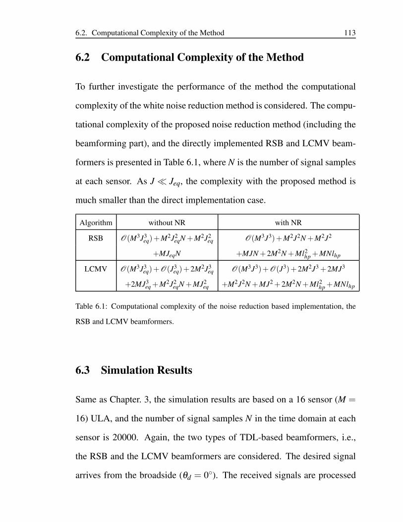
6.2. Computational Complexity of the Method 113
6.2 Computational Complexity of the Method
To further investigate the performance of the method the computational
complexity of the white noise reduction method is considered. The compu-
tational complexity of the proposed noise reduction method (including the
beamforming part), and the directly implemented RSB and LCMV beam-
formers is presented in Table 6.1, where N is the number of signal samples
at each sensor. As J ≪ Jeq, the complexity with the proposed method is
much smaller than the direct implementation case.
Algorithm without NR with NR
RSB O(M3J3eq)+M2J2
eqN +M2J2eq O(M3J3)+M2J2N +M2J2
+MJeqN +MJN +2M2N +Ml2hp +MNlhp
LCMV O(M3J3eq)+O(J3
eq)+2M2J3eq O(M3J3)+O(J3)+2M2J3 +2MJ3
+2MJ3eq +M2J2
eqN +MJ2eq +M2J2N +MJ2 +2M2N +Ml2
hp +MNlhp
Table 6.1: Computational complexity of the noise reduction based implementation, the
RSB and LCMV beamformers.
6.3 Simulation Results
Same as Chapter. 3, the simulation results are based on a 16 sensor (M =
16) ULA, and the number of signal samples N in the time domain at each
sensor is 20000. Again, the two types of TDL-based beamformers, i.e.,
the RSB and the LCMV beamformers are considered. The desired signal
arrives from the broadside (θd = 0). The received signals are processed
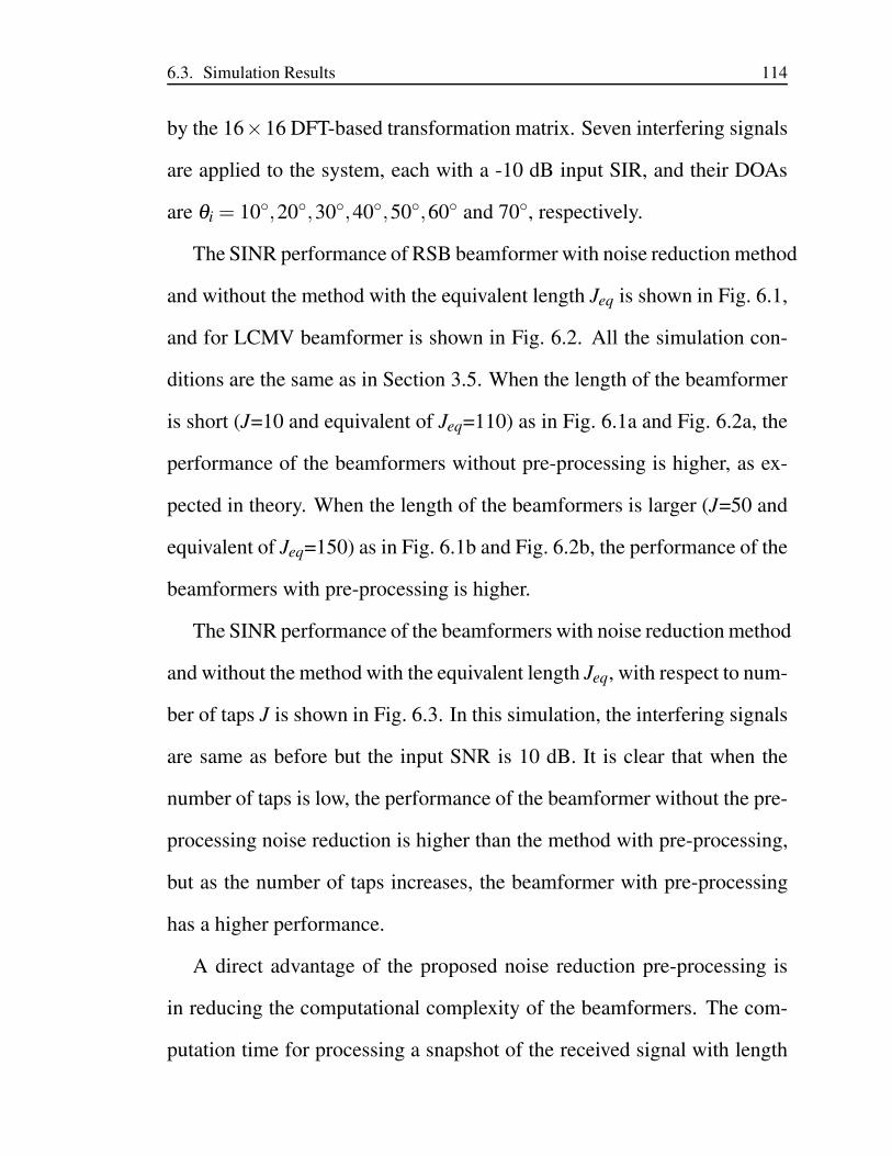
6.3. Simulation Results 114
by the 16×16 DFT-based transformation matrix. Seven interfering signals
are applied to the system, each with a -10 dB input SIR, and their DOAs
are θi = 10,20,30,40,50,60 and 70, respectively.
The SINR performance of RSB beamformer with noise reduction method
and without the method with the equivalent length Jeq is shown in Fig. 6.1,
and for LCMV beamformer is shown in Fig. 6.2. All the simulation con-
ditions are the same as in Section 3.5. When the length of the beamformer
is short (J=10 and equivalent of Jeq=110) as in Fig. 6.1a and Fig. 6.2a, the
performance of the beamformers without pre-processing is higher, as ex-
pected in theory. When the length of the beamformers is larger (J=50 and
equivalent of Jeq=150) as in Fig. 6.1b and Fig. 6.2b, the performance of the
beamformers with pre-processing is higher.
The SINR performance of the beamformers with noise reduction method
and without the method with the equivalent length Jeq, with respect to num-
ber of taps J is shown in Fig. 6.3. In this simulation, the interfering signals
are same as before but the input SNR is 10 dB. It is clear that when the
number of taps is low, the performance of the beamformer without the pre-
processing noise reduction is higher than the method with pre-processing,
but as the number of taps increases, the beamformer with pre-processing
has a higher performance.
A direct advantage of the proposed noise reduction pre-processing is
in reducing the computational complexity of the beamformers. The com-
putation time for processing a snapshot of the received signal with length
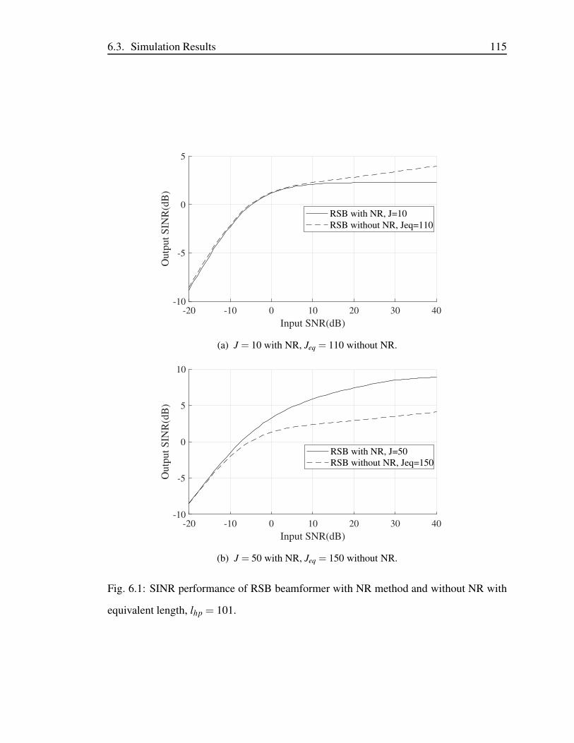
6.3. Simulation Results 115
-20 -10 0 10 20 30 40
Input SNR(dB)
-10
-5
0
5O
utp
ut
SIN
R(d
B)
RSB with NR, J=10
RSB without NR, Jeq=110
(a) J = 10 with NR, Jeq = 110 without NR.
-20 -10 0 10 20 30 40
Input SNR(dB)
-10
-5
0
5
10
Ou
tpu
t S
INR
(dB
)
RSB with NR, J=50
RSB without NR, Jeq=150
(b) J = 50 with NR, Jeq = 150 without NR.
Fig. 6.1: SINR performance of RSB beamformer with NR method and without NR with
equivalent length, lhp = 101.
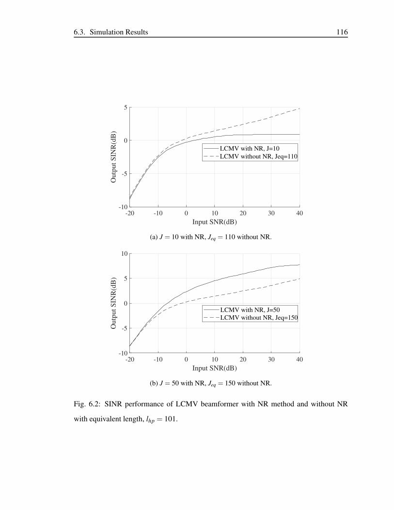
6.3. Simulation Results 116
-20 -10 0 10 20 30 40
Input SNR(dB)
-10
-5
0
5O
utp
ut
SIN
R(d
B)
LCMV with NR, J=10
LCMV without NR, Jeq=110
(a) J = 10 with NR, Jeq = 110 without NR.
-20 -10 0 10 20 30 40
Input SNR(dB)
-10
-5
0
5
10
Ou
tpu
t S
INR
(dB
)
LCMV with NR, J=50
LCMV without NR, Jeq=150
(b) J = 50 with NR, Jeq = 150 without NR.
Fig. 6.2: SINR performance of LCMV beamformer with NR method and without NR
with equivalent length, lhp = 101.
6.3. Simulation Results 117
5 10 15 20 25 30 35 40 45 50
J
-2
0
2
4
6
8
Ou
tpu
t S
INR
(dB
)
RSB with NR
RSB with Jeq
(a) RSB beamformer.
5 10 15 20 25 30 35 40 45 50
J
-2
0
2
4
6
Ou
tpu
t S
INR
(dB
)
LCMV with NR
LCMV with Jeq
(b) LCMV beamformer.
Fig. 6.3: SINR performance of both beamformers with respect to number of taps, with
NR method and without NR with equivalent length Jeq.
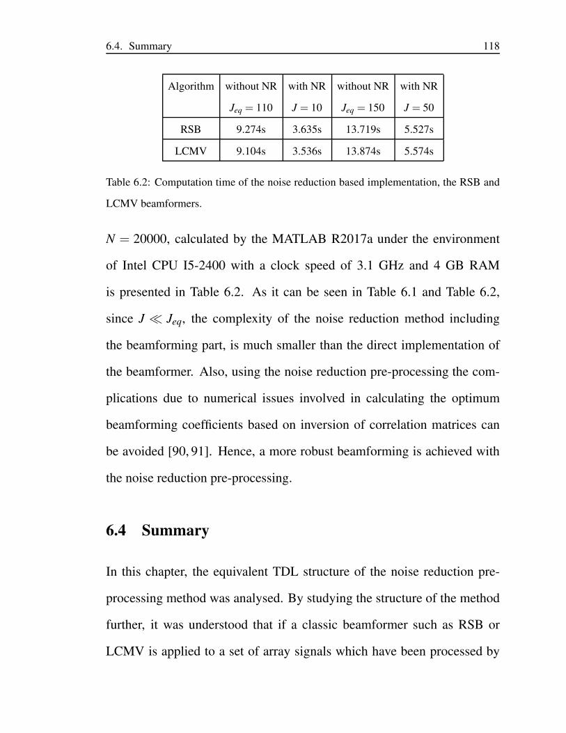
6.4. Summary 118
Algorithm without NR with NR without NR with NR
Jeq = 110 J = 10 Jeq = 150 J = 50
RSB 9.274s 3.635s 13.719s 5.527s
LCMV 9.104s 3.536s 13.874s 5.574s
Table 6.2: Computation time of the noise reduction based implementation, the RSB and
LCMV beamformers.
N = 20000, calculated by the MATLAB R2017a under the environment
of Intel CPU I5-2400 with a clock speed of 3.1 GHz and 4 GB RAM
is presented in Table 6.2. As it can be seen in Table 6.1 and Table 6.2,
since J ≪ Jeq, the complexity of the noise reduction method including
the beamforming part, is much smaller than the direct implementation of
the beamformer. Also, using the noise reduction pre-processing the com-
plications due to numerical issues involved in calculating the optimum
beamforming coefficients based on inversion of correlation matrices can
be avoided [90, 91]. Hence, a more robust beamforming is achieved with
the noise reduction pre-processing.
6.4 Summary
In this chapter, the equivalent TDL structure of the noise reduction pre-
processing method was analysed. By studying the structure of the method
further, it was understood that if a classic beamformer such as RSB or
LCMV is applied to a set of array signals which have been processed by
6.4. Summary 119
the noise reduction method, the pre-processing and the classic beamformer
can be modelled as an equivalent beamformer with longer TDLs.
The weight vector of the equivalent TDL structure was derived, and the
expressions for the computational complexity of the beamformers with and
without the noise reduction method was presented.
The advantages of using the method as a pre-processing step for the
beamformers compared to the direct usage of the classic adaptive beam-
formers with equivalent length Jeq from the viewpoint of computational
complexity was discussed, and the performance of RSB and LCMV beam-
formers with noise reduction pre-processing method, and without the method
with the equivalent length Jeq was compared by simulation results.
It was understood that the complexity of the noise reduction method in-
cluding the beamformer part is less than the direct implementation with
equivalent length Jeq. Also, with the noise reduction method, a more
robust beamforming is achieved, since by using the noise reduction pre-
processing the numerical issues due to calculating the optimum beamform-
ing coefficients based on inversion of correlation matrices are avoided.
Chapter 7
Conclusions and Future Work
7.1 Conclusions
In this thesis, a method for mitigating the effect of white noise without
affecting the directional signals in wideband arrays has been introduced.
With the proposed method, a maximum 3 dB improvement in TSNR can
be achieved in the ideal case. The increased TSNR can be translated into
performance improvement in various array signal processing applications
such as beamforming and DOA estimation.
The performance of the two well-known beamformers, namely, RSB
and LCMV beamformers was briefly reviewed in Chapter 2. The proposed
noise reduction method was introduced based on the ULA structure, and a
detailed study of the proposed method was performed in Chapter 3. The
analysis showed that the method does not have any effect on the spectra of
the directional signal in the ideal case, but it will remove half of the noise
power. Although in practice, the directional signal is distorted slightly
120
7.1. Conclusions 121
due to the presence of some signal components in lower side-lobes of the
transformation. Also, due to the limitation of the size of the array, the
improvement in TSNR is less than 3 dB.
The theoretical and simulated results for beamforming and DOA esti-
mation showed that by using the noise reduction method as a pre-processing
step, a higher output SINR performance for beamformers and a more accu-
rate DOA estimation was achieved. Since the transformation for the ULA
is unitary and the side-lobe attenuation of the DFT matrix which was used
as the transformation is as high as 13 dB, the distortion to the directional
signal caused by the method does not affect the performance considerably.
The method was re-designed to be applied to different array structures,
namely, NLA, URA and UCA.
The least squares method was employed for the design of the trans-
formation for the NLA to satisfy the required band-pass characteristics in
Chapter 4. Since the NLA has a sparse array structure, designing a unitary
or close to unitary transformation is a problematic issue. In addition to
diagonal loading, a method based on replacing the small singular values
was proposed to reduce the condition number of the transformation and
still keeping the band-pass characteristics the same. Replacing the small
singular values, reduces the condition number of the transformation which
is in our interest. The improvement in the output SINR of the RSB and
the LCMV beamformers was demonstrated by simulation. More research
is needed to successfully design unitary transformations. Since transfor-
7.1. Conclusions 122
mations which are not unitary do not preserve the power of the signal after
transformation, the transformed signals are prone to more significant dis-
tortion.
Two types of planar arrays were considered in Chapter 5, namely, URA
and UCA. Two methods for mitigating the white noise for the URA were
introduced. With the proposed method using a 2D transformation, a maxi-
mum of 1.76 dB improvement in TSNR can be achieved in the ideal case,
which is less than the 3 dB improvement achieved for the linear arrays.
Alternatively, the noise reduction method using a 1D transformation for
URAs was also proposed, which is a direct adaptation of the method used
for ULAs, with a 3 dB improvement achieved. Despite the lower TSNR,
the 2D transformation method has less distortion for the directional signals.
Therefore, depending on the application and the input SNR, either one of
the methods can provide a satisfactory performance. The transformation
was also re-designed for the UCA structure by modifying the modulation
of the row vectors of the transformation. As demonstrated by simulation
results, a clear improvement in performance, in terms of the output SINR
has been achieved for a range of input SNR values.
As it was discussed in Chapter 6, the proposed structure is equivalent
to a traditional TDL. Therefore, the noise reduction method and the cor-
responding beamformer can be considered as a beamformer with longer
TDLs, but with lower computational complexity. There are different ad-
vantages and also disadvantages of using the proposed method. Based on
7.1. Conclusions 123
the application, one might find using the method beneficial or otherwise.
Overall, some the advantages of the proposed noise reduction method
are:
• Improved TSNR by a maximum of 3 dB for different array structures.
• providing an alternative approach to beamforming with reduced com-
putational complexity.
• Achieving a more robust beamforming solution, since the method
does not involve the computation of the inverse of the signal corre-
lation matrix which is normally needed for computing the optimal
weight vector coefficients.
• Since no prior information of the impinging signal is needed, the
method is quite flexible. Therefore, it can be used for different ar-
ray signal processing applications.
On the other hand, the method has the following disadvantages:
• A unitary transformation design can only be achieved for uniform
array structures.
• For non-uniform and sparse structures, the condition number needs to
be reduced by either diagonal loading or replacing the small singular
values, which can change the beam-pattern of the transformation and
cause further complications in the design.
7.2. Future Work 124
• The noise after being processed by the method is not white any more.
This makes it more complicated to analyse the impact of the pro-
cessed noise on the performance of the array signal processing appli-
cations, such as beamforming and DOA estimation.
7.2 Future Work
The following topics can be considered as future work.
The output noise spectrum is not white after being processed by the
noise reduction processing, and it is correlated between the sensors. More
research is needed to analyse the effect of the correlated and coloured noise
on the performance of the beamformers, and the characteristics of the re-
maining noise need to be analysed further.
In Chapter 6, it was shown that the proposed structure is equivalent to
a traditional TDL system with a larger TDL length and it was mentioned
previously that the same beamforming techniques can be applied to the
new set of array signals after the proposed processing, and it is equiva-
lent to kind of adaptive beamformer but with longer TDLs. Therefore, the
proposed method can be considered as a low-complexity approach to adap-
tive beamforming. This approach can be further studied and possibly new
adaptive beamformers can be designed with lower complexity and optimal
performance.
In addition, for every array structure, a transformation was designed
7.2. Future Work 125
with the required band-pass characteristics. The transformation has to be
invertible and ideally unitary. For the ULA and URA structure design-
ing unitary transformations is not an issue, but with the increasing interest
in sparse arrays, designing a unitary transformation is challenging. The
transformation was designed for NLAs, with low condition number by ei-
ther diagonal loading or replacing the small singular values, but designing
a unitary or almost unitary transformation for sparse arrays is still an open
problem. As the array becomes more sparse, the transformation design be-
comes more difficult. Some of the sparse arrays which are in focus for fu-
ture work are co-prime arrays [92,93], nested arrays [94] and super nested
arrays [95, 96].
Another topic for further research can be designing unitary transfor-
mations with higher side-lobe attenuation. After the transformation, the
directional signals which are available on the side-lobes are removed by
consequent high-pass filters. So, the higher the side-lobe attenuation, the
less distortion is caused to the directional signal. In this thesis, for ULA, 13
dB side-lobe attenuation has been achieved with DFT matrix as the trans-
formation. By windowing techniques, higher side-lobe attenuation can be
achieved, but the transformation will not be exactly unitary after applying
the windows to the row vectors of the transformation. Therefore, further
research is needed to design unitary transformation with higher side-lobe
attenuation.
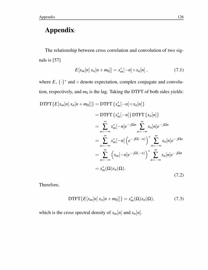
Appendix 126
Appendix:
The relationship between cross correlation and convolution of two sig-
nals is [57]
E[xm[n] xn[n+m0]] = x∗m[−n] xn[n] , (7.1)
where E, ·∗ and denote expectation, complex conjugate and convolu-
tion, respectively, and m0 is the lag. Taking the DTFT of both sides yields:
DTFTE[xm[n] xn[n+m0]]= DTFTx∗m[−n] xn[n]
= DTFTx∗m[−n]DTFTxn[n]
=∞
∑n=−∞
x∗m[−n]e− jΩn∞
∑n=−∞
xn[n]e− jΩn
=∞
∑n=−∞
x∗m[−n](
e− jΩ(−n))∗ ∞
∑n=−∞
xn[n]e− jΩn
=∞
∑n=−∞
(
xm[−n]e− jΩ(−n))∗ ∞
∑n=−∞
xn[n]e− jΩn
= x∗m(Ω)xn(Ω).
(7.2)
Therefore,
DTFTE[xm[n] xn[n+m0]]= x∗m(Ω)xn(Ω), (7.3)
which is the cross spectral density of xm[n] and xn[n].
Bibliography
[1] H. L. Van Trees, Optimum Array Processing, Part IV of Detection,
Estimation, and Modulation Theory, Wiley, New York, April 2002.
[2] W. Liu and S. Weiss, Wideband Beamforming: Concepts and Tech-
niques, John Wiley & Sons, Chichester, UK, March 2010.
[3] H. Krim and M. Viberg, “Two decades of array signal processing re-
search: the parametric approach,” IEEE Signal Processing Magazine,
vol. 13, no. 4, pp. 67–94, July 1996.
[4] B. Allen and M. Ghavami, Adaptive Array Systems, Fundamentals
and Applications, John Wiley & Sons, Chichester, England, February
2005.
[5] W. Yang, Sensor Array, InTech, DOI: 10.5772/2034, March 2012.
[6] B. Widrow, J. R. Glover, J. M. McCool, J. Kaunitz, C. S. Williams,
R. H. Hearn, J. R. Zeidler, J. E. Dong, and R. C. Goodlin, “Adaptive
noise cancelling: Principles and applications,” Proceedings of the
IEEE, vol. 63, no. 12, pp. 1692–1716, December 1975.
127
Bibliography 128
[7] A. K. Jain, Fundamentals of digital image processing, Prentice-Hall,
Inc., January 1989.
[8] H. Ogawa and E. Oja, “Projection filter, Wiener filter, and
Karhunen-Loeve subspaces in digital image restoration,” Journal of
Mathematical analysis and applications, vol. 114, no. 1, pp. 37–51,
February 1986.
[9] Y. Kamamori, A. Kawamura, and Y. Liguni, “Zero phase signal anal-
ysis and its application to noise reduction,” IEICE Transactions on
Fundamentals of Electronics, Communications and Computer Sci-
ences, vol. J93-A, pp. 658–666, October 2010.
[10] S. Kohmura, A. Kawamura, and Y. Iiguni, “An efficient zero phase
noise reduction method for impact noise with damped oscillation,”
in Proc. IEEE International Conference on Acoustics, Speech, and
Signal Processing, Vancouver, BC, Canada, 26 May 2013, IEEE, pp.
892–895.
[11] T. B. Spalt, C. R. Fuller, T. F. Brooks, and W. Humphreys, “A
background noise reduction technique using adaptive noise cancel-
lation for microphone arrays,” in Proc. 17th AIAA/CEAS Aeroacous-
tics Conference, American Institute of Aeronautics and Astronautics,
Portland, OR, 6 June 2011, pp. 2715–2731.
Bibliography 129
[12] J. Chen, J. Benesty, Y. Huang, and S. Doclo, “New insights into the
noise reduction Wiener filter,” IEEE Transactions on audio, speech,
and language processing, vol. 14, no. 4, pp. 1218–1234, July 2006.
[13] J. S. Goldstein, I. S. Reed, and L. L. Scharf, “A multistage repre-
sentation of the Wiener filter based on orthogonal projections,” IEEE
Transactions on Information Theory, vol. 44, no. 7, pp. 2943–2959,
November 1998.
[14] S. Kohmura, A. Kawamura, and Y. Iiguni, “A zero phase noise reduc-
tion method with damped oscillation estimator,” IEICE Transactions
on Fundamentals of Electronics, Communications and Computer Sci-
ences, vol. 97, no. 10, pp. 2033–2042, October 2014.
[15] W. Thanhikam, Y. Kamamori, A. Kawamura, and Y. Iiguni, “Station-
ary and non-stationary wide-band noise reduction using zero phase
signal,” IEICE Transactions on Fundamentals of Electronics, Com-
munications and Computer Sciences, vol. 95, no. 5, pp. 843–852,
May 2012.
[16] A. Tanaka and A. Kawamura, “Iterative zero phase method for white
and impulse noise reduction,” in Proc. 22nd International Conference
on Digital Signal Processing (DSP), London, UK, 23 August 2017,
IEEE, pp. 1–5.
Bibliography 130
[17] R. Schmidt, “Multiple emitter location and signal parameter estima-
tion,” IEEE Transactions on Antennas and Propagation, vol. 34, pp.
276–280, March 1986.
[18] R. Roy and T. Kailath, “ESPRIT-estimation of signal parameters
via rotational invariancetechniques,” IEEE Transactions on Acous-
tics, Speech, and Signal Processing, vol. 37, no. 7, pp. 984–995, July
1989.
[19] B. Friedlander and A. J. Weiss, “Direction finding for wide-band
signals using an interpolated array,” IEEE Transactions on Signal
Processing, vol. 41, no. 4, pp. 1618–1634, April 1993.
[20] J. Krolik and D. Swingler, “Focused wide-band array processing by
spatial resampling,,” IEEE Transactions on Acoustics, Speech, and
Signal Processing, vol. 38, no. 2, pp. 356–360, February 1990.
[21] G. Su and M. Morf, “The signal subspace approach for multiple wide-
band emitter location,” IEEE Transactions on Acoustics, Speech and
Signal Processing, vol. 31, no. 6, pp. 1502–1522, December 1983.
[22] H. Wang and M. Kaveh, “Coherent signal-subspace processing for
the detection and estimation of angles of arrival of multiple wide-
band sources,” IEEE Transactions on Acoustics, Speech, and Signal
Processing, vol. 33, pp. 823–831, August 1985.
Bibliography 131
[23] Y.-S Yoon, L. M. Kaplan, and J. H. McClellan, “TOPS: new DOA
estimator for wideband signals,” IEEE Transactions on Signal Pro-
cessing, vol. 54, no. 6, pp. 1977–1989, June 2006.
[24] E. J. Candes, J. Romberg, and T. Tao, “Robust uncertainty principles:
exact signal reconstruction from highly incomplete frequency infor-
mation,” IEEE Transactions on Information Theory, vol. 52, no. 2,
pp. 489 – 509, February 2006.
[25] E. J. Candes, M. B. Wakin, and S. P. Boyd, “Enhancing sparsity by
reweighted l1 minimization,” Journal of Fourier Analysis and Appli-
cations, vol. 14, pp. 877–905, December 2008.
[26] D. Malioutov, M. Cetin, and A. S. Willsky, “A sparse signal re-
construction perspective for source localization with sensor arrays,”
IEEE Transactions on Signal Processing, vol. 53, no. 8, pp. 3010–
3022, August 2005.
[27] J. H. Yin and T. Q. Chen, “Direction-of-arrival estimation using a
sparse representation of array covariance vectors,” IEEE Transactions
on Signal Processing, vol. 59, no. 9, pp. 4489–4493, September 2011.
[28] J. M. Zheng and M. Kaveh, “Sparse spatial spectral estimation: a
covariance fitting algorithm, performance and regularization,” IEEE
Transactions on Signal Processing, vol. 61, no. 11, pp. 2767–2777,
June 2013.
Bibliography 132
[29] Y. M. Zhang, M. G. Amin, and B. Himed, “Sparsity-based DOA es-
timation using co-prime arrays,” in Proc. IEEE International Con-
ference on Acoustics, Speech, and Signal Processing, Vancouver,
Canada, May 2013, pp. 3967–3971.
[30] Z. M. Liu, Z. T. Huang, and Y. Y. Zhou, “Direction-of-arrival esti-
mation of wideband signals via covariance matrix sparse representa-
tion,” IEEE Transactions on Signal Processing, vol. 59, no. 9, pp.
4256–4270, Sept. 2011.
[31] Z.-M. Liu, Z.-T. Huang, and Y.-Y. Zhou, “Sparsity-inducing direction
finding for narrowband and wideband signals based on array covari-
ance vectors,” IEEE Transactions on Wireless Communications, vol.
12, no. 8, pp. 1–12, August 2013.
[32] Q. Shen, W. Liu, W. Cui, S. L. Wu, Y. D. Zhang, and M. Amin,
“Low-complexity direction-of-arrival estimation based on wideband
co-prime arrays,” IEEE Trans. Audio, Speech and Language Process-
ing, vol. 23, pp. 1445–1456, September 2015.
[33] V. Ambegaokar and B. I. Halperin, “Voltage due to thermal noise in
the dc josephson effect,” Physical Review Letters, vol. 22, no. 25, pp.
1364, June 1969.
[34] H. Nyquist, “Thermal agitation of electric charge in conductors,”
Physical review, vol. 32, no. 1, pp. 110, July 1928.
Bibliography 133
[35] Y. M. Blanter and M. Buttiker, “Shot noise in mesoscopic conduc-
tors,” Physics reports, vol. 336, no. 1-2, pp. 1–166, October 2000.
[36] R. H. Dicke, P. J. E. Peebles, P. G. Roll, and D. T. Wilkinson,
“Cosmic Black-Body Radiation,” The Astrophysical Journal, vol.
142, pp. 414–419, July 1965.
[37] C. Kipnis and S. R. S. Varadhan, “Central limit theorem for additive
functionals of reversible markov processes and applications to simple
exclusions,” Communications in Mathematical Physics, vol. 104, no.
1, pp. 1–19, January 1986.
[38] W. Liu and R. J. Langley, “An adaptive wideband beamforming struc-
ture with combined subband decomposition,” IEEE Transactions on
Antennas and Propagation, vol. 89, pp. 913–920, July 2009.
[39] R. T. Compton, Jr., “The relationship between tapped delay-line and
FFT processing in adaptive arrays,” IEEE Transactions on Antennas
and Propagation, vol. 36, no. 1, pp. 15–26, January 1988.
[40] R. T. Compton, “The bandwidth performance of a two-element adap-
tive array with tapped delay-line processing,” IEEE Transactions on
Antennas and Propagation, vol. 36, no. 1, pp. 4–14, January 1988.
[41] A. Jakobsson, S. R. Alty, and S. Lambotharan, “On the implemen-
tation of the linearly constrained minimum variance beamformer,”
Bibliography 134
IEEE Transactions on Circuits & Systems II: Express Briefs, vol. 53,
no. 10, pp. 1059–1062, October 2006.
[42] M. E. Knox, “Single antenna full duplex communications using a
common carrier,” in Wireless and microwave technology conference
(WAMICON), 2012 IEEE 13th annual, Cocoa Beach, FL, USA, 15-
17 April 2012, IEEE, pp. 1–6.
[43] D. Yang, G. Xue, J. Zhang, A. Richa, and X. Fang, “Coping with a
smart jammer in wireless networks: A stackelberg game approach,”
IEEE Transactions on Wireless Communications, vol. 12, no. 8, pp.
4038–4047, August 2013.
[44] S. R. Best, “The receiving and scattering properties of a finite dipole
array,” IEEE Antennas and Propagation Magazine, vol. 53, no. 6, pp.
9–17, December 2011.
[45] M. Wang, L. Lin, J. Chen, D. Jackson, W. Kainz, Y. Qi, and P. Jar-
muszewski, “Evaluation and optimization of the specific absorption
rate for multiantenna systems,” IEEE Transactions on Electromag-
netic Compatibility, vol. 53, no. 3, pp. 628–637, August 2011.
[46] L. Cohen, “The generalization of the Wiener-Khinchin theorem,”
in Proceedings of the IEEE International Conference on Acoustics,
Speech and Signal Processing. IEEE, 15 May 1998, vol. 3, pp. 1577–
1580.
Bibliography 135
[47] M. S. Brandstein and D. Ward, Eds., Microphone Arrays: Signal Pro-
cessing Techniques and Applications, Springer, Berlin, April 2001.
[48] W. E. Rodgers and R. T. Compton, Jr., “Adaptive array bandwidth
with tapped delay-line processing,” IEEE Trans. Areospace Elec-
tronic Systems, vol. AES-15, no. 1, pp. 21–27, January 1979.
[49] O. L. Frost, III, “An algorithm for linearly constrained adaptive array
processing,” Proceedings of the IEEE, vol. 60, no. 8, pp. 926–935,
August 1972.
[50] M. R. Anbiyaei, W. Liu, and D. C. McLernon, “White noise reduction
for wideband linear array signal processing,” IET Signal Processing,
October 2017.
[51] M. R. Anbiyaei, W. Liu, and D. C. McLernon, “Performance im-
provement for wideband DOA estimation with white noise reduction
based on uniform linear arrays,” in Proc. IEEE, Sensor Array and
Multichannel Signal Processing Workshop (SAM), Rio de Janeiro,
Brazil, July 2016.
[52] B. Noble and J. W. Daniel, Applied Linear Algebra, Prentice-Hall,
Upper Saddle River, NJ, 1977.
[53] W. Liu, S. Weiss, and L. Hanzo, “A subband-selective broadband
GSC with cosine-modulated blocking matrix,” IEEE Transactions on
Antennas and Propagation, vol. 52, pp. 813–820, March 2004.
Bibliography 136
[54] T. Sekiguchi and Y. Karasawa, “Wideband beamspace adaptive array
utilizing FIR fan filters for multibeam forming,” IEEE Transactions
on Signal Processing, vol. 48, no. 1, pp. 277–284, January 2000.
[55] W. Liu, R. Wu, and R. Langley, “Design and analysis of broadband
beamspace adaptive arrays,” IEEE Transactions on Antennas and
Propagation, vol. 55, no. 12, pp. 3413–3420, December 2007.
[56] B. Mulgrew, P. Grant, and J. Thompson, “Random signal analysis,”
in Digital Signal Processing, pp. 176–205. Macmillan Education UK,
1999.
[57] R. N. Bracewell, The Fourier Transform and its applications,
McGraw-Hill Series in Electrical Engineering, Networks and Sys-
tems, New York, 2nd edition, February 1986.
[58] E. J. Candes and T. Tao, “Near-optimal signal recovery from random
projections: Universal encoding strategies,” IEEE transactions on
Information Theory, vol. 52, no. 12, pp. 5406–5425, 30 November
2006.
[59] C. Y. Chen and P. P. Vaidyanathan, “Compressed sensing in MIMO
radar,” in Proc. 42nd Asilomar Conference on Signals, Systems and
Computers. IEEE, October 2008, pp. 41–44.
Bibliography 137
[60] N. B. Karahanoglu and H. Erdogan, “A* orthogonal matching pursuit:
Best-first search for compressed sensing signal recovery,” Digital
Signal Processing, vol. 22, no. 4, pp. 555–568, July 2012.
[61] S. S. Chen, D. L. Donoho, and M. A. Saunders, “Atomic decompo-
sition by basis pursuit,” SIAM review, vol. 43, no. 1, pp. 129–159,
2001.
[62] J. A. Tropp and S. J. Wright, “Computational methods for sparse
solution of linear inverse problems,” Proceedings of the IEEE, vol.
98, no. 6, pp. 948–958, April 2010.
[63] M. Rossi, A. M. Haimovich, and Y. C. Eldar, “Conditions for target
recovery in spatial compressive sensing for MIMO radar,” in Proc.
IEEE International Conference on Acoustics, Speech and Signal Pro-
cessing (ICASSP). IEEE, May 2013, pp. 4115–4119.
[64] J. Kim, R. Monteiro, and H. Park, “Group sparsity in nonnegative
matrix factorization,” in Proc. SIAM International Conference on
Data Mining, Anaheim, CA, USA, 2012, SIAM, pp. 851–862.
[65] J. Huang and T. Zhang, “The benefit of group sparsity,” The Annals
of Statistics, vol. 38, no. 4, pp. 1978–2004, 2010.
[66] M. Grant and S. Boyd, “CVX: Matlab software for disciplined con-
vex programming, version 2.0 beta, build 1023,” December 2013,
Available: http://cvxr.com/cvx.
Bibliography 138
[67] M. Grant and S. Boyd, “Graph implementations for nonsmooth con-
vex programs,” in Recent Advances in Learning and Control, V. Blon-
del, S. Boyd, and H. Kimura, Eds., Lecture Notes in Control and
Information Sciences, pp. 95–110. Springer-Verlag Limited, 2008,
http://stanford.edu/ boyd/graph dcp.html.
[68] P. Stoica and A. Nehorai, “MUSIC, maximum likelihood, and
Cramer-Rao bound,” IEEE Transactions on Acoustics, Speech, and
Signal Processing, vol. 37, no. 5, pp. 720–741, May 1989.
[69] B. D. Carlson, “Covariance matrix estimation errors and diagonal
loading in adaptive arrays,” IEEE Transactions on Aerospace and
Electronic Systems, vol. 24, pp. 397–401, July 1988.
[70] F. W. Vook and R. T. Compton, Jr., “Bandwidth performance of lin-
ear adaptive arrays with tapped delay-line processing,” IEEE Trans-
actions on Aerospace and Electronic Systems, vol. 28, no. 3, pp. 901–
908, July 1992.
[71] N. Lin, W. Liu, and R. J. Langley, “Performance analysis of an adap-
tive broadband beamformer based on a two-element linear array with
sensor delay-line processing,” Signal Processing, vol. 90, pp. 269–
281, January 2010.
[72] M. R. Anbiyaei, W. Liu, and D. C. McLernon, “Performance im-
provement for wideband beamforming with white noise reduction
Bibliography 139
based on sparse arrays,” in Proc. 25th European Signal Processing
Conference (EUSIPCO), Kos Island, Greece, Aug 2017, pp. 2433–
2437.
[73] Y. Zhao, W. Liu, and R. J. Langley, “An application of the least
squares approach to fixed beamformer design with frequency invari-
ant constraints,” IET Signal Processing, pp. 281–291, June 2011.
[74] M. B. Hawes and W. Liu, “Sparse microphone array design for wide-
band beamforming,” in Proc. International Conference on Digital
Signal Processing, Santorini, Greece, July 2013.
[75] R. L. de Queiroz, “On unitary transform approximations,” IEEE
Signal Processing Letters, vol. 5, no. 2, pp. 46–47, February 1998.
[76] R. L. de Queiroz, “Approximating lapped transforms through unitary
postprocessing,” IEEE Signal Processing Letters, vol. 8, no. 12, pp.
307–309, December 2001.
[77] M. Ghavami, “Wideband smart antenna theory using rectangular ar-
ray structures,” IEEE Transactions on Signal Processing, vol. 50, no.
9, pp. 2143–2151, September 2002.
[78] W. Liu, “Design and implementation of a rectangular frequency in-
variant beamformer with a full azimuth angle coverage,” Journal of
the Franklin Institute, vol. 348, pp. 2556–2569, November 2011.
Bibliography 140
[79] S. C. Chan and K. S. Pun, “On the design of digital broadband beam-
former for uniform circular array with frequency invariant charac-
teristics,” in Proc. IEEE International Symposium on Circuits and
Systems, Phoenix, USA, May 2002, vol. 1, pp. 693–696.
[80] L. Yu and W. Liu, “Performance analysis of the data subtraction
based robust beamformer,” in Proc. of the Sensor Signal Processing
for Defence Conference, London, UK, September 2011, pp. 21–24.
[81] M. R. Anbiyaei, W. Liu, and D. C. McLernon, “White noise reduction
for wideband beamforming based on uniform rectangular arrays,” in
Proc. 22nd International Conference on Digital Signal Processing
(DSP), London, UK, Aug 2017, pp. 1–5.
[82] G. Sommerkorn, D. Hampicke, R. Klukas, A. Richter, A. Schneider,
and R. Thoma, “Uniform rectangular antenna array design and cal-
ibration issues for 2-d ESPRIT application,” in Proceedings of the
4th European Personal Mobile Communications Conference, Vienna,
Austria, February 2001.
[83] J. S. Lim and A. V. Oppenheim, Two-dimensional Signal and Image
Processing, Prentice Hall, Englewood Cliffs, New Jersey, 1990.
[84] W. Liu, “Design of a rectangular frequency invariant beamformer
with a full azimuth angle coverage,” in Proc. European Signal Pro-
cessing Conference, Glasgow, Scotland, August 2009, pp. 579–582.
Bibliography 141
[85] P. Ioannides and C. A. Balanis, “Uniform circular and rectangular
arrays for adaptive beamforming applications,” IEEE Antennas and
Wireless Propagation Letters, vol. 4, no. 1, pp. 351–354, 26 Septem-
ber 2005.
[86] C. A. Balanis, Antenna Theory: Analysis and Design, Wiley, Febru-
ary 2016.
[87] M. Abramowitz and I. A. Stegun, Eds., Handbook of Mathematical
Functions, Dover Publications, New York, 1970.
[88] P. S. Naidu, Sensor array signal processing, CRC press, June 2009.
[89] C. P. Robert, Monte Carlo Methods, Wiley Online Library, August
2016.
[90] P. C. Hansen, Rank-Deficient and Discrete Ill-Posed Problems. Nu-
merical Aspects of Linear Inversion, SIAM, Philadelphia, 1998.
[91] C. R. Vogel, Computational Methods for Inverse Problems, Soci-
ety for Industrial and Applied Mathematics, Philadelphia, PA, USA,
2002.
[92] P. P. Vaidyanathan and P. Pal, “Sparse sensing with co-prime samplers
and arrays,” IEEE Transactions on Signal Processing, vol. 59, no. 2,
pp. 573–586, Feb. 2011.
[93] S. Qin, Y. D. Zhang, and M. G. Amin, “Generalized coprime ar-
ray configurations for direction-of-arrival estimation,” IEEE Trans-
Bibliography 142
actions on Signal Processing, vol. 63, no. 6, pp. 1377–1390, March
2015.
[94] P. Pal and P. P. Vaidyanathan, “Nested arrays: A novel approach to
array processing with enhanced degrees of freedom,” IEEE Trans-
actions on Signal Processing, vol. 58, no. 8, pp. 4167–4181, August
2010.
[95] C. L. Liu and P. P. Vaidyanathan, “Super nested arrays: Linear sparse
arrays with reduced mutual coupling—Part I: Fundamentals,” IEEE
Transactions on Signal Processing, vol. 64, no. 15, pp. 3997–4012,
August 2016.
[96] C. L. Liu and P. P. Vaidyanathan, “Super nested arrays: Linear
sparse arrays with reduced mutual coupling—Part II: High-order ex-
tensions,” IEEE Transactions on Signal Processing, vol. 64, no. 16,
pp. 4203–4217, August 2016.


![DESIGN OF A WIDEBAND VIVALDI ANTENNA ARRAY … · DESIGN OF A WIDEBAND VIVALDI ANTENNA ARRAY ... Two double-ridged waveguide TEM horn antennas ... Double transition in HFSS[R]](https://img.pdfslide.us/doc/110x75/5ae77def7f8b9a3d3b8e9763/design-of-a-wideband-vivaldi-antenna-array-of-a-wideband-vivaldi-antenna-array.jpg)