Embed Size (px)
Citation preview
JOURNAL OF GEOPHYSICAL RESEARCH, VOL. 85, NO. C10, PAGES 5529-5554, OCTOBER 20, 1980
Sensitivity of a Global Climate Model to an Increase of CO2 Concentration in the Atmosphere
SYUKURO MANABE AND RONALD J. STOUFFER
Geophysical Fluid Dynamics Laboratory/NOAA, Princeton University, Princeton, New Jersey 08540
This study investigates the response of a global model of the climate to the quadrupling of the CO2 concentration in the atmosphere. The model consists of (1) a general circulation model of the atmo- sphere, (2) a heat and water balance model of the continents, and (3) a simple mixed layer model of the oceans. It has a global computational domain and realistic geography. For the computation of radiative transfer, the seasonal variation of insolation is imposed at the top of the model atmosphere, and the fixed distribution of cloud cover is prescribed as a function of latitude and of height. It is found that with some exceptions, the model succeeds in reproducing the large-scale characteristics of seasonal and geographi- cal variation of the observed atmospheric temperature. The climatic effect of a CO2 increase is deter- mined by comparing statistical equilibrium states of the model atmosphere with a normal concentration and with a 4 times the normal concentration of CO2 in the air. It is found that the warming of the model atmosphere resulting from the CO2 increase has significant seasonal and latitudinal variation. Because of the absence of an albedo feedback mechanism, the warming over the Antarctic continent is somewhat less than the warming in high latitudes of the northern hemisphere. Over the Arctic Ocean and its sur- roundings, the warming is much larger in winter than summer, thereby reducing the amplitude of sea- sonal temperature variation. It is concluded that this seasonal asymmetry in the warming results from the reduction in the coverage and thickness of the sea ice. The warming of the model atmosphere results in an enrichment of the moisture content in the air and an increase in the poleward moisture transport. The additional moisture is picked up from the tropical ocean and is brought to high latitudes where both pre- cipitation and runoff increase throughout the year. Further, the time of rapid snowmelt and maximum runoff becomes earlier.
1. INTRODUCTION
Since the pioneering work of Callender [1938], many studies have been made on the climatic impact of an anthropogenic increase in the CO2 concentration in the atmosphere. Earlier studies of this topic [Plass, 1956; Kondratiev and Niilisk, 1960; Kaplan, 1960; M611er, 1963] contain an evaluation of the tem- perature change at the earth's surface in response to an in- crease of the CO2 concentration based upon the consideration of the surface radiation balance. One of the basic short-
comings of this approach is that it cannot properly incorpo- rate the influence of the atmospheric heat balance upon the temperature change of the earth's surface. As was demon- strated by M611er [1963], this approach leads to rather unre- liable results.
Manabe and Wetheraid [1967] avoided this difficulty by us- ing a radiative convective equilibrium model of the atmo- sphere in which the heat exchanges among the earth's surface, atmosphere, and outer space are taken into consideration. Studies of the climate sensitivity problem with radiative con- vective equilibrium models are extensively reviewed by Ra- manathan and Coakley [1978]. Refer to their review for some of the latest results from this approach.
Obviously, a radiative convective model is a highly sim- plified model of the atmosphere and does not contain some of the important dynamical and physical processes such as the snow-albedo feedback mechanism and the dynamics of the large-scale atmospheric circulation. To evaluate the response of the atmosphere to a CO2 increase considering these proc- esses, Manabe and Wetherald [1975, 1980] used a general cir- culation model of the atmosphere with a limited computa- tional domain, idealized geography, and annual mean
This paper is not subject to U.S. copyright. Published in 1980 by the American Geophysical Union.
insolation. They conducted extensive studies of the thermal, dynamical, and hydrological response of the model.
The present study is a natural extension of the studies by Manabe and Wetheraid. It investigates the CO2 climate sensi- tivity problem by use of a global circulation model of the at- mosphere with a simple mixed layer ocean, realistic geogra- phy, and seasonal variation of insolation. In the interpretation of the results from this model, one should recognize that the additional complexity of the model does not necessarily guar- antee the better simulation of the sensitivity of the actual cli- mate. However, it is hoped that the present study identifies some specific mechanisms controlling the sensitivity of the cli- mate. Special emphasis of the study is placed upon the investi- gation of the seasonal and interhemispheric asymmetries in the response of the model climate to an increase of the CO2 concentration in the air. Some of the results from this study were summarized briefly in an earlier publication by Manabe and $touffer [ 1979].
2. MODEL STRUCTURE
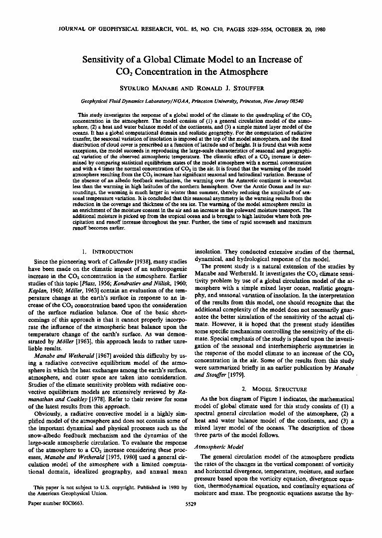
As the box diagram of Figure I indicates, the mathematical model of global climate used for this study consists of (1) a spectral general circulation model of the atmosphere, (2) a heat and water balance model of the continents, and (3) a mixed layer model of the oceans. The description of those three parts of the model follows.
Atmospheric Model
The general circulation model of the atmosphere predicts the rates of the changes in the vertical component of vorticity and horizontal divergence, temperature, moisture, and surface pressure based upon the vorticity equation, divergence equa- tion, thermodynamical equation, and continuity equations of moisture and mass. The prognostic equations assume the by-
Paper number 80C0663. 5529
5530 MANABE AND STOUFFER.' GLOBAL CLIMATE MODEL OF CO 2 INCREASE
ATMOSPHERE
CONTINUITY THERMODYNAMIC EQUATION OF EQUATION
,
WATER VAPOR RADIATION
EQUATION OF MOTION
HYDROLOGY ,HEAT BALANCE I
CONTINENT
SEA ICE ,HEAT BALANCE i
MIXEB LAYER OCEAN Fig. 1. Box diagram illustrating the basic structure of the mathematical model of global climate.
drostatic approximation and use a variable, o = [(Pressure)/ (surface pressure)], as the vertical coordinate for the conve- nience of incorporating the effect of surface topography [Phil- lips, 1957].
The horizontal distributions of the aforementioned vari-
ables are represented by a finite number of spherical harmon- ics. The model predicts the rate of change of the spectral com- ponents by computing the tendencies from the prognostic equations at all grid points and by transforming them to the spectral domain. This transform method originally proposed by Orsag [1970] and Eliassen et al. [1970] yields an accuracy comparable with the conventional spectral method [e.g., Platzman, 1960]. It also consumes much less computer time than the latter when the spectral resolution of a model is high. Obviously, the horizontal resolution of a spectral representa- tion of a field depends upon the degree of spectral truncation. For the present model, so-called rhomboidal truncation is used. Fifteen waves are retained in both longitudinal and meridional directions. The vertical derivatives appearing in the prognostic equations are computed by a finite difference method. The model has nine unevenly spaced finite difference levels in the vertical where o = 0.025, 0.095, 0.205, 0.350, 0.515, 0.680, 0.830, 0.940, and 0.990.
The numerical time integration of the prognostic equations are conducted by a semi-implicit method in which the linear and nonlinear components of the rate of change of a variable are separated and are time-integrated implicitly and explicitly, respectively. To prevent the growth of fictitious computational solutions, a time-smoothing technique developed by Robert [1966] is applied at each time step. The smoothing constant a is chosen to be 0.02.
The dynamical component of the model described above is developed by Gordon and Stern [1974] and is very similar to the spectral model developed by Bourke [1974] and Hoskins and Simmons [1975]. The reader is referred to these papers for further details. The performance of this spectral model of the atmosphere general circulation is evaluated in detail by Ma- nabe et al. [1979b].
The physical processes incorporated into the model are nearly identical with those used in the general circulation model of Holloway and Manabe [1971]. A brief description of these processes follows.
Condensation of water vapor is predicted whenever super- saturation is indicated in the prognostic equation of water va- por. Snowfall is predicted when the air temperature at an alti- tude of 300 m falls below the freezing temperature. Otherwise, rainfall is predicted. Refer to Manabe et al. [1965] for further details of prognostic system of water vapor.
For the computation of terrestrial radiation, a scheme of Rodgers and Walshaw [1966] as modified by Stone and Ma- nabe [1968] is used. For the computation of solar radiation flux, the scheme developed by Lacis and Hansen [1974] is used after minor modification. The seasonal and latitudinal varia-
tion of insolation is prescribed at the top of the model atmo- sphere. For the sake of simplicity, the diurnal variation is re- moved from the insolation. The depletion of solar radiation and the transfer of terrestrial radiation is computed by taking into consideration the effects of clouds, water vapor, carbon dioxide, and ozone. The mixing ratio of carbon dioxide is as- sumed to be constant everywhere. A zonally uniform distribu- tion of ozone is specified as a function of latitude, height, and season by use of the data compiled by Hering and Borden [1964] and London [1962]. Cloud cover is assumed to be zo- nally uniform and invariant with respect to time. The annual mean distribution of cloud cover used for this study is deter- mined based upon the studies of London [1957] and $asamori and London [1972]. The distribution of water vapor is deter- mined from the time integration of the prognostic equation of water vapor.
Heat and Water Balance Model of the Continents
Surface temperatures over the continents are determined by the boundary condition that no heat is stored in the soil (i.e., the net fluxes of solar and terrestrial radiation and the turbu-
lent fluxes of sensible and latent heat locally add to zero). For the computation of the net downward flux of solar radiation, the surface albedos are prescribed as a function of latitude over oceans and geographically over continents based upon the study of Posey and Clapp [1964]. However, these albedos are replaced by higher values whenever snow cover or sea ice are simulated.
The albedos for snow cover are mainly determined by lati- tude and the snow depth. Table 1 gives the albedo values for deep snow as a function of latitude. When the snow depth is
MANABE AND STOUFFER: GLOBAL CLIMATE MODEL OF CO 2 INCREASE 5531
TABLE 1. Albedo (%) as Function of Latitude for Snow and Sea Ice
Degrees Latitude
0ø-55 o 55 ø-66.5 o 66.5 ø-90ø
Deep snow 60 60 --- 80* 80 Thick sea ice 50 50 --- 70 70
*--- means linear interpolation with respect to latitude between the two values.
below a critical value equivalent to 1 cm of precipitable water, the albedos are reduced. Referring to the study by Kung et al. [1964], it is assumed that snow albedo decreases from the val- ues in Table I to the lower albedo of underlying soil suface as a square root function of snow depth (represented in water equivalent). Note that the albedo of the snow-free surface over the Greenland and Antarctic ice sheets is almost as large as the albedo for deep snow so that there is little albedo feed- back when the snow melts.
The change of soil moisture is computed from the rates of rainfall, evaporation, snowmelt, and runoff. A change of snow depth is predicted as a net contribution from snowfall, sub- limation, and snowmelt, the last being determined from the heat budget requirement. For further details of the hydrologic computations over the continental surface, refer to Manabe [1969a].
Mixed Layer Ocean Model
It is well known that the oceans have a far reaching influ- ence upon climate. Oceans are the source of moisture for the hydrologic cycle. The oceans also have a large heat capacity and thus reduce the amplitude of the seasonal temperature variation. In addition, ocean currents influence climate through horizontal heat transport. The mixed layer model of ocean used for this study includes the first two of these three influences but lacks the third one, the horizontal heat trans- port. The sensitivity of a climate model, which incorporates a three-dimensional ocean model with ocean currents, is the subject of future investigation.
In this study the mixed layer of the ocean is simplified as a vertically isothermal layer of static water with uniform thick- ness. Over the ice-free region, the prognostic equation for the mixed layer temperature Tm is
OTto Q • -- (1)
at Co' H
where Co is the heat capacity of water, and H is the thickness of the mixed layer ocean. Q, the rate of net heat gain by the ocean, is defined by the following equation
Q --/red- fSH- fLH (2)
where fred is the flux of net downward radiation (including both solar and terrestrial radiation), fsH and fLH are upward fluxes of sensible and latent heat, respectively. The heat ex- change between the mixed layer and the deeper layers of the oceans is not taken into consideration.
Over the ice covered region, the temperature of the mixed layer ocean remains at the freezing point (i.e., -2øC). Thus the rate of its change is zero.
The albedo of the mixed layer ocean, necessary for the computation of the net radiation flux at the ocean surface, is prescribed as a function of latitude. When the ocean is cov-
ered by sea ice, a higher value of surface albedo is assigned. Table I gives the albedo values for thick sea ice as a function of latitude. When the thickness of ice is less than 50 cm, the albedo decreases from the values in Table I to the lower al-
bedo of underlying water surface as a square root function of ice thickness. The sea ice albedo of Table 1 is further reduced
to 45% when the top surface of the sea ice is melting; this in- corporates the influence of fresh water ponds (or puddles) forming on top Of the ice pack.
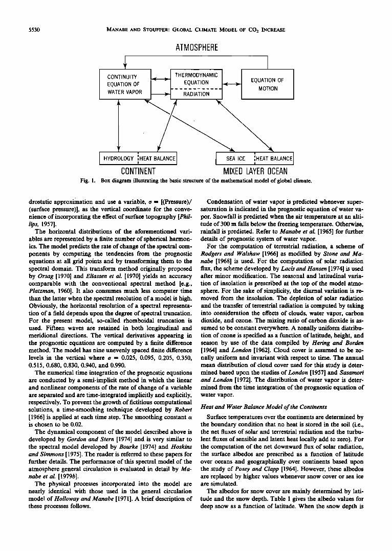
The thickness of the mixed layer is chosen such that it is equal to the effective depth of the seasonal thermocline Df which is defined by the following equation
Df' AAT-•-O- • = AAT-• x dz = A.• T(z) x dz (3)
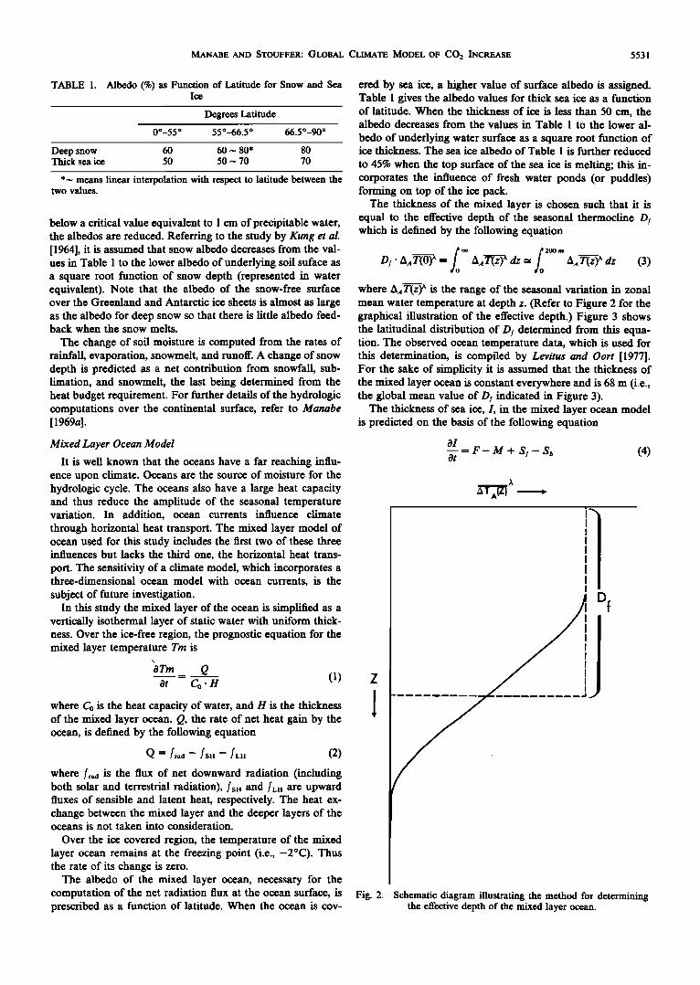
where A• T(z) x is the range of the seasonal variation in zonal mean water temperature at depth z. (Refer to Figure 2 for the graphical illustration of the effective depth.) Figure 3 shows the latitudinal distribution of D• determined from this equa- tion. The observed ocean temperature data, which is used for this determination, is compiled by Levitus and Oort [1977]. For the sake of simplicity it is assumed that the thickness of the mixed layer ocean is constant everywhere and is 68 m (i.e., the global mean value of D• indicated in Figure 3).
The thickness of sea ice, L in the mixed layer ocean model is predicted on the basis of the following equation
0I --= F- M + S•- Sb (4) Ot
aT A(ZJ
i
Fig. 2. Schematic diagram illustrating the method for determining the effective depth of the mixed layer ocean.
5532 MANABE AND STOUFFER: GLOBAL CLIMATE MODEL OF CO 2 INCREASE
50
100
150 I , I • I I • I I • , I , [ I [ • 90N 60 30 0 30 60 90S
LATITUDE
Fig. 3. Latitudinal distribution of the effective depth of the mixed layer ocean as determined by the method illustrated in Figure 2.
where Sf and So denote the rates of snowfall and sub- limination (in water equivalent). M and F are rates of melting and freezing of sea ice, respectively. In this equation the effect of ice advection by wind stress and ocean currents is not taken into consideration. In the presence of sea ice, the temperature of the mixed layer ocean is at the freezing point, and the heat conduction through the sea ice is balanced by the latent heat of freezing or melting at the bottom of the sea ice. The freez- ing and melting at the ice bottom, together with the melting at the ice top, sublimation, and snowfall determines the change of ice thickness. For further details, see Bryan [1969] and Ma- nabe [1969b].
3. NUMERICAL EXPERIMENTS
The climatic impacts of an increase in the CO2 content of the atmosphere are investigated based upon a comparison be- tween the climate of the model with the normal concentration
of CO2 (i.e., 300 ppm) and another model climate with 4 times the normal concentration (i.e., 1200 ppm). One could have in- vestigated the consequences of a smaller difference in the CO2 concentration. Instead, the CO2 content is altered by a sub- stantial factor for ease of discriminating the CO2 induced change from the natural fluctuation of the model climate [Leith, 1973]. Following the normal practice, the climates with the normal and with 4 times the normal CO2 concentrations are obtained from the long-term integrations of the model de- scribed in the preceding section. (Hereafter, these two in- tegrations are identified as the 1 x CO2 and 4 x CO2 experi-
TABLE 2. Length and Number of Seasonal Cycles in Each Stage of the Numerical Time Integrations
Length of Seasonal Cycle, Year Number of
Atmosphere Ocean Seasonal Cycles
I X GO 2 Experiment •/• 1 4 •/8 1 1 1/4 1 1 '/2 ! 1 ! ! 5
4 X C02 Experiment 1/16 1 4 1/8 1 1 1/4 1 1 •/• 1 2 1 1 6
ments, respectively.) It is found that the period of numerical time integration required for the model to settle down to a stable climatic condition is approximately 10-15 years. Since the straightforward integration of the model consumes a large amount of computer time and is therefore very costly, an eco- nomical method of time integration is developed.
For the development of an economical method, it is impor- tant to recognize the following characteristics of a joint ocean- atmosphere model. (1) The thermal inertia of the atmospheric part of the model is much shorter than that of the oceanic part. (2) The numerical time integration of the atmospheric model over a given time period usually consumes much more computer time than that of the oceanic model. With these fac- tors in mind, Manabe and Bryan [1969] developed an econom- ical method in which a very long-term integration of the oce- anic part of the joint model is synchronized with a relatively short-term integration of the atmospheric part of the model. Thus they reduced the disparity between the two parts of the model in approaching toward a statistically stationary climate. The consequence is a shortening of the period of atmospheric integration by a substantial factor.
For the present study their method is modified such that it is applicable to the time integration of the joint model with seasonal variation of insolation. In this modified version the
time integration of the atmospheric part of the model over the period of an accelerated seasonal cycle is synchronized with a full 1 year integration of the oceanic part of the model. At the beginning of the integration, the period of the accelerated sea- sonal cycle for the atmospheric model is chosen to be 1/16 of a year (i.e., 365/16 = 23 days). The period increases in several steps and becomes a full year (i.e., 365 days) toward the end of the integration. Table 2 tabulates the length and number of the atmospheric seasonal cycles for each experiment.
During a time integration, the quantities which are trans- reitted from the atmospheric to the oceanic part of the joint model are the exchange rates of momentum, heat, water, and ice (including snow). On the other hand, the distributions of sea surface temperature and sea ice thickness are transmitted from the oceanic to the atmospheric part of the model. For further details of the information exchange, refer' to Manabe [ 1969b] and Bryan [ 1969].
The present economical method used in this study' differs from an earlier economical method, which is developed by Manabe et al. [1979a] for the seasonal time integration of a joint model with a deep ocean. It is found that the earlier method is not effective in accelerating the approach of the
MANABE AND STOUFFER: GLOBAL CLIMATE MODEL OF CO 2 INCREASE 5533
2
300
2g0
280
270
260
250
24O
_ • LW TOP
_ \
• SW TOP
230 I I I I I I I I I I I I I 1 2 3 4 5 6 7 8 9 10 11 12 13
YEARS
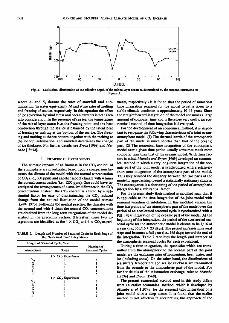
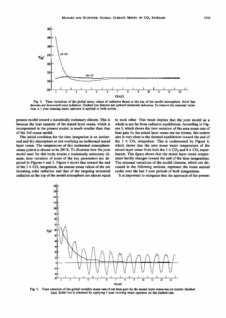
Fig. 4. Time variations of the global mean values of radiative fluxes at the top of the model atmosphere. Solid line denotes net downward solar radiation. Dashed line denotes net upward terrestrial radiation. To remove the seasonal varia- tion, a 1 year running mean operator is applied to both curves.
present model toward a statistically stationary climate. This is because the heat capacity of the mixed layer ocean, which is incorporated in the present model, is much smaller than that of the full ocean model.
The initial condition for the time integration is an isother- mal and dry atmosphere at rest overlying an isothermal mixed layer ocean. The temperature of this isothermal atmosphere- ocean system is chosen to be 280 K. To illustrate how the joint model used for this study attains a statistically stationary cli- mate, time variation of some of the key parameters are de- picted in Figures 4 and 5. Figure 4 shows that toward the end of the 1 x CO2 integration, the annual mean values of the net incoming solar radiation and that of the outgoing terrestrial radiation at the top of the model atmosphere are almost equal
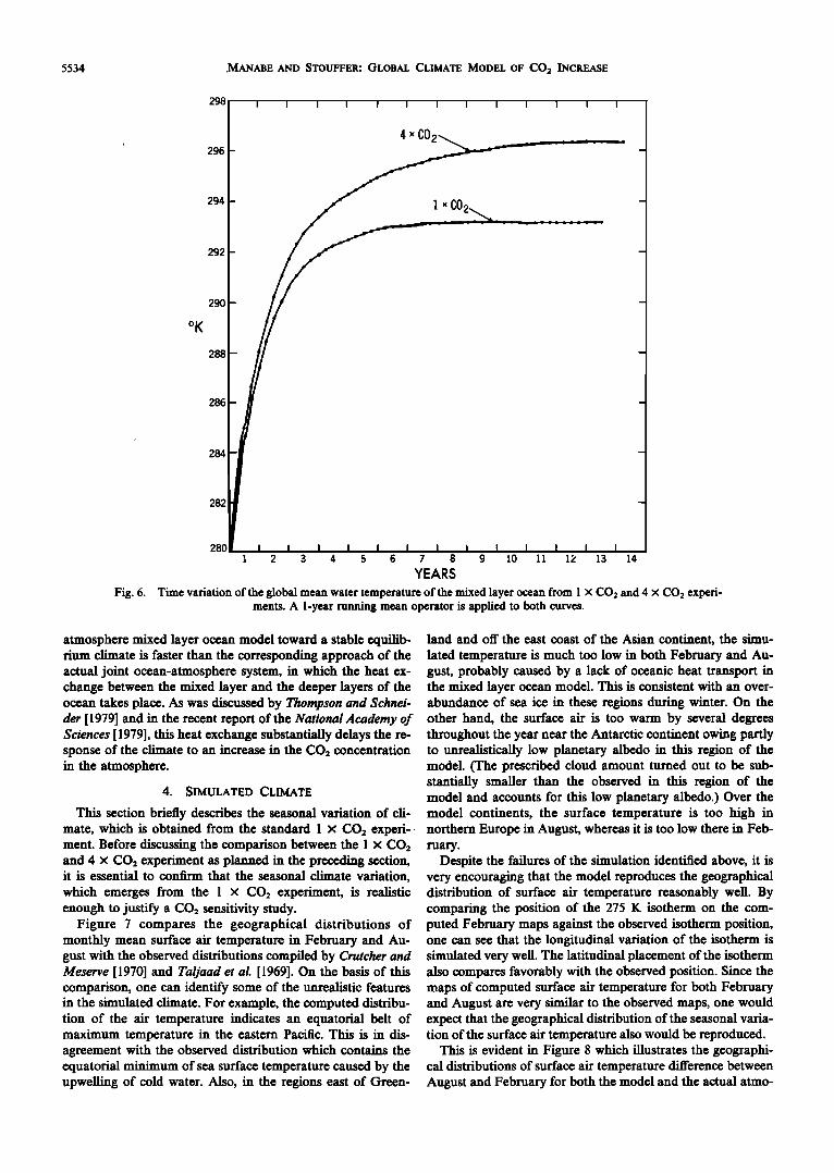
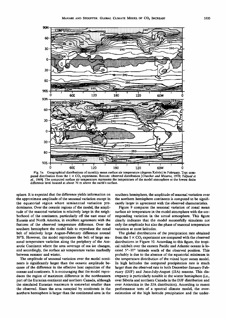
to each other. This result implies that the joint model as a whole is not far from radiative equilibrium. According to Fig- ure 5, which shows the time variation of the area mean rate of heat gain by the mixed layer ocean-sea ice system, this system also is very close to the thermal equilibrium toward the end of the 1 x CO2 integration. This is underscored by Figure 6, which shows that the area mean water temperature of the mixed layer ocean from both the 1 x CO: and 4 x CO2 exper- iments. This figure shows that the mixed layer ocean temper- ature hardly changes toward the end of the time integrations. The seasonal variations of the model climates, which are dis- cussed in the following sections, represent the mean annual cycles over the last 3 year periods of both integrations.
It is important to recognize that the approach of the present
140
130
120
110
100
9O
8O
7O
W/M 60 5O
4O
3O
2O
lO
0--
-10
-20
-30
t I \i
-- i X w • .'•
, , , , ,. ,, /, ,-, ,, ,,, ,., / • ' I I ' t I I t ' ' e' J I ' I - t , , , , , , , , , , , , ,
'] ' I I I I I I t ' I t I • I I t I • • tt I I I I • I I I t I I I I I I I t I i I
I I I I I I I I I I I I I 1 2 3 4 5 6 7 8 9 10 ll 12 13
YEARS
Fig. 5. Time va•ation of the global monthly mean rate of net heat gain by the m•ed layer ocean-sea ice system (dashed line). Solid line is obtained by applying 1 year •ng mean operator on the dashed line.
5534 ,MANABE AND STOUFFER: GLOBAL CLIMATE MODEL OF CO2 INCREASE
296
I I I I I I I I I' I I I I
4,• CO,
294 1 ,,CO,
292
290
o K
288
286
284
282
28o 1 2 3 4 5 6 7 8 9 1o 11 12 13 14
YEARS
Fig. 6. Time variation of the global mean water temperature of the mixed layer ocean from I x CO2 and 4 x CO2 experi- ments. A l-year running mean operator is applied to both curves.
atmosphere mixed layer ocean model toward a stable equilib- land and off the east coast of the Asian continent, the simu- rium climate is faster than the corresponding approach of the lated temperature is much too low in both February and Au- actual joint ocean-atmosphere system, in which the heat ex- gust, probably caused by a lack of oceanic heat transport in change between the mixed layer and the deeper layers of the the mixed layer ocean model. This is consistent with an over- ocean takes place. As was discussed by Thompson and $chnei- abundance of sea ice in these regions during winter. On the der [1979] and in the recent report of the National Academy of other hand, the surface air is too warm by several degrees Sciences [1979], this heat exchange substantially delays the re- sponse of the climate to an increase in the CO• concentration in the atmosphere.
4. SIMULATED CLIMATE
This section briefly describes the seasonal variation of eli-
throughout the year near the Antarctic continent owing partly to unrealistically low planetary albedo in this region of the model. (The prescribed cloud amount turned out to be sub- stantially smaller than the observed in this region of the model and accounts for this low planetary albedo.) Over the model continents, the surface temperature is too high in
mate, which is obtained from the standard 1 x CO• experi-, northern Europe in August, whereas it is too low there in Feb- ment. Before discussing the comparison between the 1 x CO• ruary. and 4 x CO• experiment as planned in the preceding section, Despite the failures of the simulation identified above, it is it is essential to confirm that the seasonal climate variation, very encouraging that the model reproduces the geographical which emerges from the 1 x CO2 experiment, is realistic distribution of surface air temperature reasonably well. By enough to justify a CO2 sensitivity study. comparing the position of the 275 K isotherm on the com-
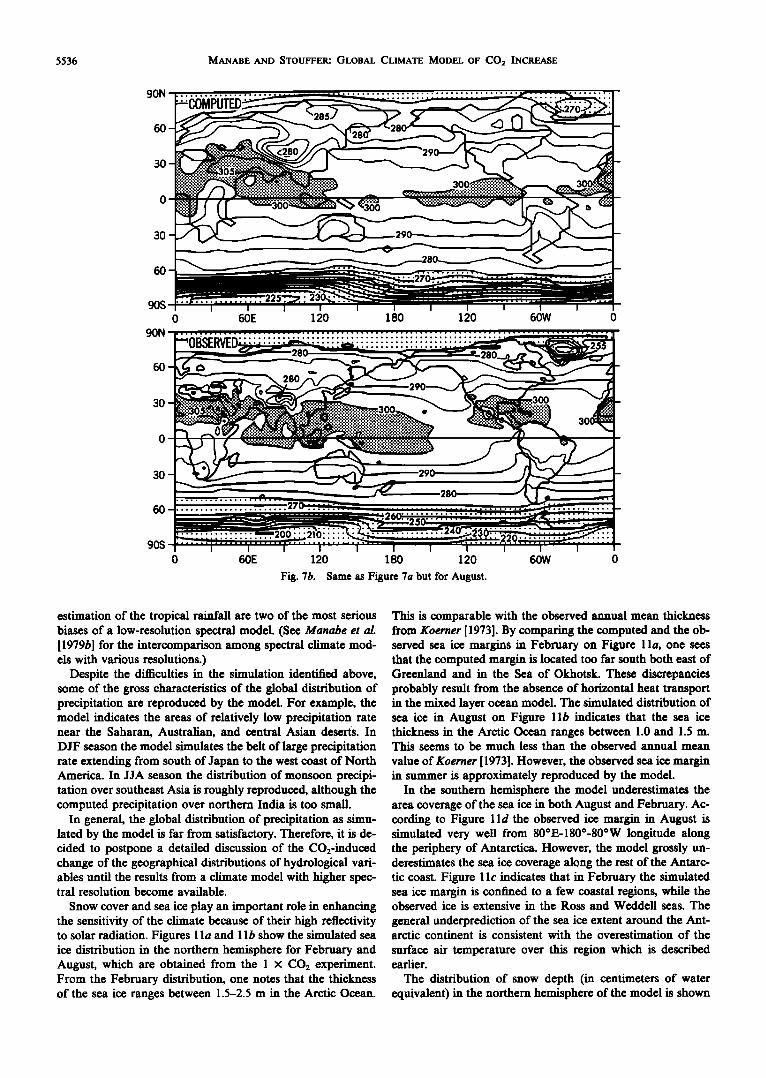
Figure 7 compares the geographical distributions of puted February maps against the observed isotherm position, monthly mean surface air temperature in February and Au- gust with the observed distributions compiled by Crutcher and Meserve [1970] and Taljaad et al. [1969]. On the basis of this comparison, one can identify some of the unrealistic features in the simulated climate. For example, the computed distribu- tion of the air temperature indicates an equatorial belt of maximum temperature in the eastern Pacific. This is in dis- agreement with the observed distribution which contains the equatorial minimum of sea surface temperature caused by the upwelling of cold water. Also, in the regions east of Green-
one can see that the longitudinal variation of the isotherm is simulated very well. The latitudinal placement of the isotherm also compares favorably with the observed position. Since the maps of computed surface air temperature for both February and August are very similar to the observed maps, one would expect that the geographical distribution of the seasonal varia- tion of the surface air temperature also would be reproduced.
This is evident in Figure 8 which illustrates the geographi- cal distributions of surface air temperature difference between August and February for both the model and the actual atmo-
MANABE AND STOUFFER: GLOBAL CLIMATE MODEL OF CO2 INCREASE 5535
90N
60
30 290
30
60
90S
90N
60
30
30
60
90S
0 60E 120 180 120 60W 0
300
280
0 60E 120 180 120 60W 0
Fig. 7a. Geographical distributions of monthly mean surface air temperature (degrees Kelvin) in February. Top: com- puted distribution from the I x CO2 experiment. Bottom: observed distribution [Crutcher and Meserve, 1970; Taljaad et al., 1969]. The computed surface air temperature represents the temperature of the model atmosphere at the lowest finite difference level located at about 70 m above the earth's surface.
sphere. It is expected that the difference yields information on the approximate amplitude of the seasonal variation except in the equatorial region where semiannual variation pre- dominates. Over the oceanic regions of the model, the ampli- tude of the seasonal variation is relatively large in the neigh- borhood of the continents, particularly off the east coast of Eurasia and North America, in excellent agreement with the features of the observed temperature difference. Over the southern hemisphere the model fails to reproduce the zonal belt of relatively large August-February difference around 30øS. However, the model reproduces the belt of large sea- sonal temperature variation along the periphery of the Ant- arctic Continent where the area coverage of sea ice changes, and accordingly, the surface air temperature varies markedly between summer and winter.
The amplitude of seasonal variation over the model conti- nents is significantly larger than the oceanic amplitude be- cause of the difference in the effective heat capacities of the oceans and continents. It is encouraging that the model repro- duces the region of maximum difference in the northeastern part of the Eurasian continent and northern Canada, although the simulated Eurasian maximum is somewhat smaller than
the observed. Since the area occupied by continents in the northern hemisphere is larger than the continental area in the
southern hemisphere, the amplitude of seasonal variation over the northern hemisphere continents is computed to be signifi- cantly larger in agreement with the observed characteristics.
Figure 9 compares the seasonal variation of zonal mean surface air temperature in the model atmosphere with the cor- responding variation in the actual atmosphere. This figure clearly indicates that the model successfully simulates not only the amplitude but also the phase of seasonal temperature variation at most latitudes.
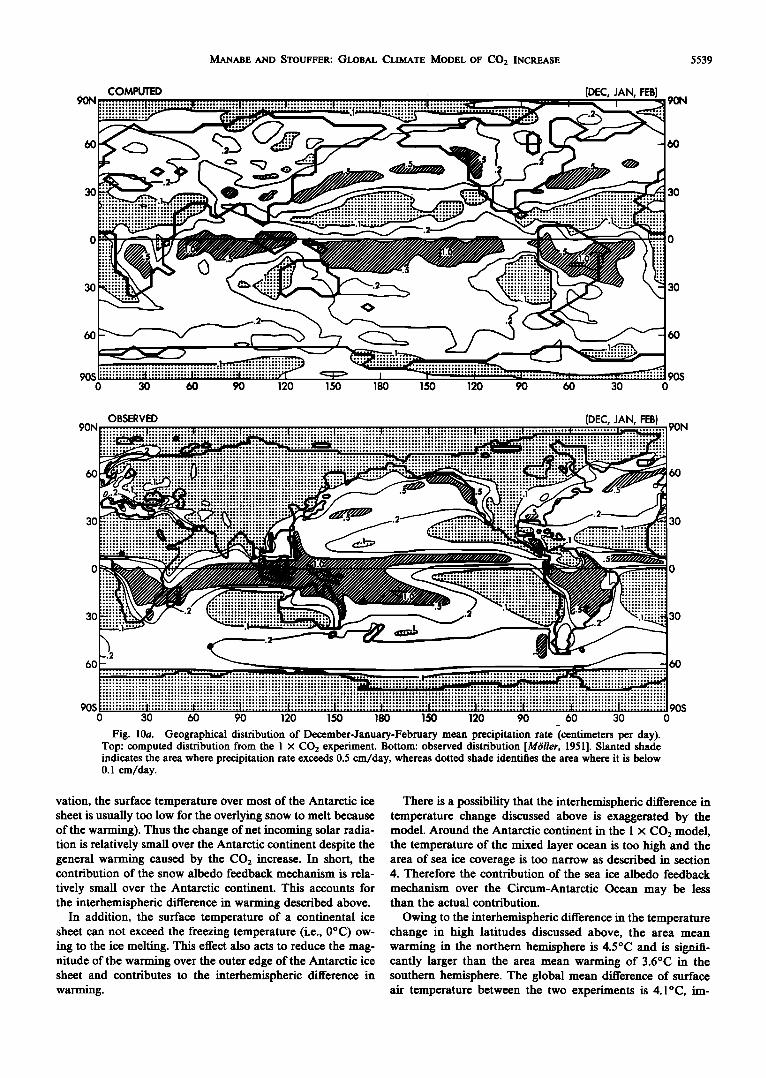
The global distributions of the precipitation rate obtained from the 1 x CO2 experiment are compared with the observed distributions in Figure 10. According to this figure, the tropi- cal rainbelt over the eastern Pacific and Atlantic oceans is lo-
cated 5ø-10 ø latitude south of the observed position. This probably is due to the absence of the equatorial minimum in the temperature distribution of the mixed layer ocean model. In high latitudes the computed precipitation rate is much larger than the observed rate in both December-January-Feb- ruary (DJF) and June-July-August (JJA) seasons. This dis- crepancy is particularly notable in the winter hemisphere (i.e., over Siberia and northern Canada in the DJF distribution and
over Antarctica in the JJA distribution). According to recent performance tests of a spectral climate model, the over- estimation of the high latitude precipitation and the under-
5536 MANABE AND STOUFFER: GLOBAL CLIMATE MODEL OF CO2 INCREASE
90N
60
30
30
60
90S
90N
60
30
30
60
300
60E 120 180 120 60W
280
90S
0 60E 120 180 120
Fig. 7b. Same as Figure 7a but for August.
60W o
estimation of the tropical rainfall are two of the most serious biases of a low-resolution spectral model. (See Manabe et al. [1979b] for the intercomparison among spectral climate mod- els with various resolutions.)
Despite the difficulties in the simulation identified above, some of the gross characteristics of the global distribution of precipitation are reproduced by the model. For example, the model indicates the areas of relatively low precipitation rate near the Saharan, Australian, and central Asian deserts. In DJF season the model simulates the belt of large precipitation rate extending from south of Japan to the west coast of North America. In JJA season the distribution of monsoon precipi- tation over southeast Asia is roughly reproduced, although the computed precipitation over northern India is too small.
In general, the global distribution of precipitation as simu- lated by the model is far from satisfactory. Therefore, it is de- cided to postpone a detailed discussion of the CO2-induced change of the geographical distributions of hydrological vari- ables until the results from a climate model with higher spec- tral resolution become available.
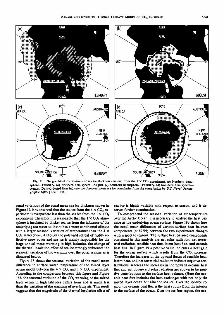
Snow cover and sea ice play an important role in enhancing the sensitivity of the climate because of their high reflectivity to solar radiation. Figures 1 la and I lb show the simulated sea ice distribution in the northern hemisphere for February and August, which are obtained from the I x CO2 experiment. From the February distribution, one notes that the thickness of the sea ice ranges between 1.5-2.5 m in the Arctic Ocean.
This is comparable with the observed annual mean thickness from Koerner [1973]. By comparing the computed and the ob- served sea ice margins in February on Figure 1 la, one sees that the computed margin is located too far south both east of Greenland and in the Sea of Okhotsk. These discrepancies probably result from the absence of horizontal heat transport in the mixed layer ocean model. The simulated distribution of sea ice in August on Figure lib indicates that the sea ice thickness in the Arctic Ocean ranges between 1.0 and 1.5 m. This seems to be much less than the observed annual mean
value of Koerner [ 1973]. However, the observed sea ice margin in summer is approximately reproduced by the model.
In the southern hemisphere the model underestimates the area coverage of the sea ice in both August and February. Ac- cording to Figure 1 ld the observed ice margin in August is simulated very well from 80øE-180ø-80øW longitude along the periphery of Antarctica. However, the model grossly un- derestimates the sea ice coverage along the rest of the Antarc- tic coast. Figure 1 l c indicates that in February the simulated sea ice margin is confined to a few coastal regions, while the observed ice is extensive in the Ross and Weddell seas. The
general underprediction of the sea ice extent around the Ant- arctic continent is consistent with the overestimation of the
surface air temperature over this region which is described earlier.
The distribution of snow depth (in centimeters of water equivalent) in the northern hemisphere of the model is shown
MANABE AND STOUFFER: GLOBAL CLIMATE MODEL OF CO 2 INCREASE 5537
90N
60
30
30
60
90S
90N 0 60E 120 180 120 60W 0
60
30
30
60
90S
0 60E 120 180 120 60W 0
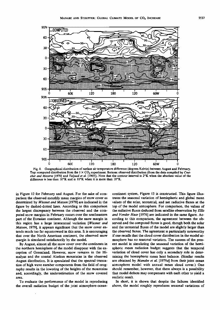
Fig. 8. Geographical distribution of surface air temperature difference (degrees Kelvin) between August and February. Top: computed distribution from the I x CO2 experiment. Bottom: observed distribution (from the data compiled by Crut- cher and Meserve [1970] and Taljaad et al. [1969]). Note that the contour interval is 2øK when the absolute value of the difference is less than 10øK and is 10øK when it is more than 10øK.
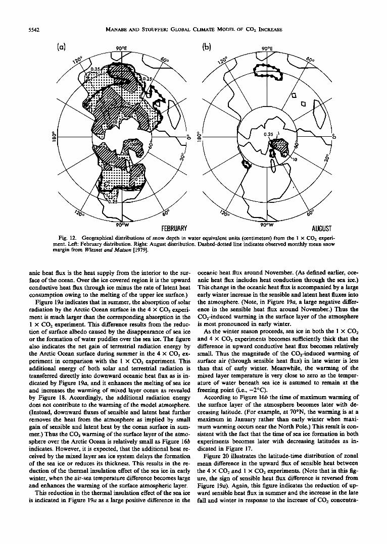
in Figure 12 for February and August. For the sake of com- parison the observed monthly mean margins of snow cover as determined by Wiesnet and Matson [1979] are indicated in the figure by dashed-dotted lines. According to this comparison the largest discrepancy between the observed and the com- puted snow margins in February occurs over the southeastern part of the Eurasian continent. Although the snow margin in this region has a large interannual variation [Wiesnet and Matson, 1979], it appears significant that the snow cover ex- tends much too far equatorward in this area. It is encouraging that over the North American continent, the observed snow margin is simulated satisfactorily by the model.
By August, almost all the snow cover over the continents in the northern hemisphere of the model disappear with the ex- ception of Greenland. However, snow remains in the Hi- malyas and the coastal Alaskan mountains in the observed August distribution. It is speculated that the spectral trunca- tion of high wave number components from the field of orog- raphy results in the lowering of the heights of the mountains and, accordingly, the underestimation of the snow covered area.
To evaluate the performance of the model in reproducing the overall radiation budget of the joint atmosphere-ocean-
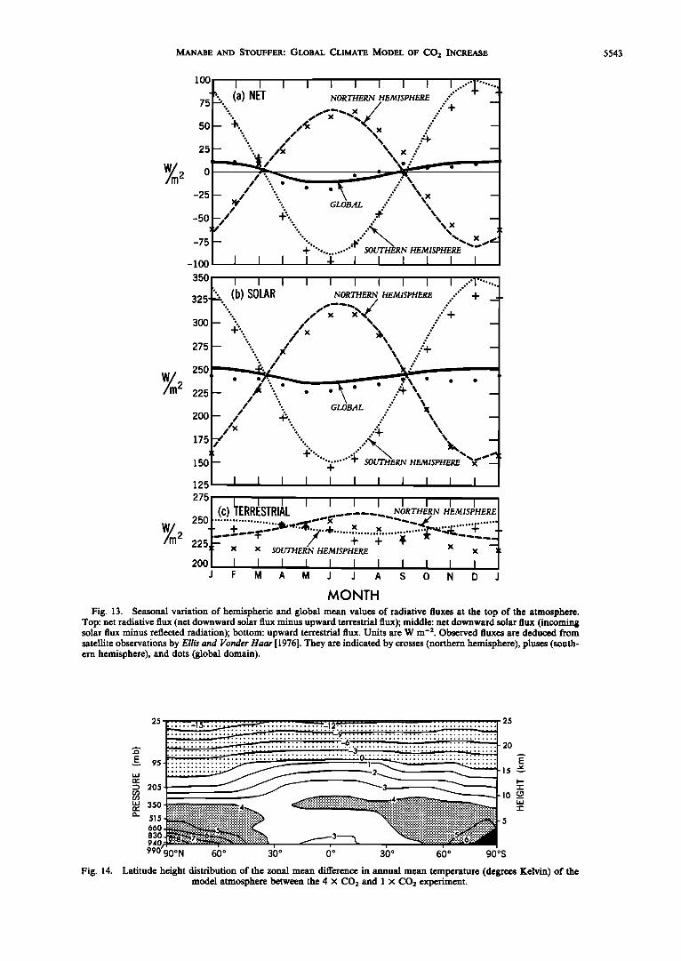
continent system, Figure 13 is constructed. This figure illus- trates the seasonal variation of hemispheric and global mean values of the solar, terrestrial, and net radiative fluxes at the top of the model atmosphere. For comparison, the values of the radiative fluxes deduced from satellite observation by Ellis and Vonder Haar [1976] are indicated in the same figure. Ac- cording to this comparison, the agreement between the ob- served and the computed fluxes is good, though both the solar and the terrestrial fluxes of the model are slightly larger than the observed fluxes. The agreement is particularly noteworthy if one recalls that the cloud cover distribution in the model at-
mosphere has no seasonal variation. The success of the pres- ent model in simulating the seasonal variation of the hemi- spheric mean radiation budget suggests that the temporal variation of cloud cover has only a secondary role in deter- mining the hemispheric mean heat balance. (Similar results are obtained by Manabe et al. [1979a] from their joint ocean atmosphere model with annual mean cloud cover.) One should remember, however, that there always is a possibility that model defects may compensate with each other to yield a realistic result.
In short, it is shown that despite the failures identified above, the model roughly reproduces seasonal variations of
5538 MANABE AND STOUFFER.' GLOBAL CLIMATE MODEL OF CO 2 INCREASE
90øN
60 ø
30 ø
o
30 ø
0
,90øS
Jan Apr Jul Oct Jan Jan Apr Jul Oct Jan
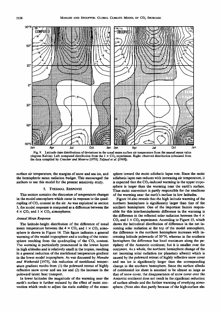
Fig. 9. Latitude-time distributions of deviations in the zonal mean surface air temperature from the am•ua! mean value (degrees Kelvin). Left: computed distribution from the 1 x CO2 experiment. Right: observed distribution (obtained from the data compiled by Crutcher and Meserve [1970]; Taljaad et al. [1969]).
surface air temperature, the margins of snow and sea ice, and the hemispheric mean radiation budget. This encouraged the authors to use this model for the present sensitivity study.
5. THERMAL RESPONSE
This section contains the discussion of temperature changes in the model atmosphere which occur in response to the quad- rupling of CO2 content in the air. As was explained in section 3, the model response is computed as a difference between the 4 x CO: and I x CO: atmospheres.
Annual Mean Response
The latitude-height distribution of the difference of zonal mean temperature between the 4 x CO: and 1 x CO: atmo- sphere is shown in Figure 14. This figure indicates a general warming of the model troposphere and a cooling of the strato- sphere resulting from the quadrupling of the CO2 content. The warming is particularly pronounced in the lowest layers in high altitudes and is relatively small in the tropics, resulting in a general reduction of the meridional temperature gradient in the lower model troposphere. As was discussed by Manabe and Wetheraid [1975], this reduction of meridional temper- ature gradient results from (1) the poleward retreat of highly reflective snow cover and sea ice and (2) the increase in the poleward latent heat transport.
In lower latitudes the magnitude of the warming near the earth's surface is further reduced by the effect of moist con- vection which tends to adjust the static stability of the atmo-
sphere toward the moist adiabatic lapse rate. Since the moist adiabatic lapse rate reduces with increasing air temperature, it is expected that the CO:-induced warming in the upper tropo- sphere is larger than the warming near the earth's surface. Thus moist convection is partly responsible for the smallness of the warming near the earth's surface in low latitudes.
Figure 14 also reveals that the high latitude warming of the northern hemisphere is significantly larger than that of the southern hemisphere. One of the important factors respon- sible for this interhemisphereic difference in the warming is the difference in the reflected solar radiation between the 4 x
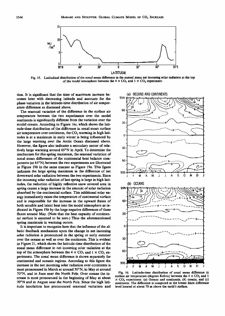
CO: and 1 x CO: experiment. According to Figure 15, which shows the latitudinal distribution of difference in the net in-
coming solar radiation at the top of the model atmosphere, the difference in the northern hemisphere increases with in- creasing latitude polewards of 30øN, whereas in the southern hemisphere the difference has local maximum along the pe- riphery of the Antarctic continent, but it is smaller over the continent. As a whole, the northern hemisphere change of the net incoming solar radiation (or planetary albedo) which is caused by the poleward retreat of highly reflective snow cover and sea ice is significantly larger than the corresponding change in the southern hemisphere. Since the surface albedo of continental ice sheet is assumed to be almost as large as that of snow cover, the disappearance of snow cover over the Antarctic continent does not result in the significant reduction of surface albedo and the further warming of overlying atmo- sphere. (Note also that partly because of the high-surface ele-
MANABE AND STOUFFER: GLOBAL CLIMATE MODEL OF CO 2 INCREASE 5539
90N
30
COMPUTED (DEC, JAN, FEB) 90N
30
30
60
90S o 30 60 90 120 150 180 150 120 90 60 30
30
905 0
90N
60
30
30
60
90S 0
OBSERVED
::::::::::::::::::::::::::::::::::::::: .......
:::::::::::::::::::::::::::::::::
::iii:::::::: •
::::::::::::::::
(DEC, JAN, FEB)
....... :::: .................... ..
:::::::::::::::::
............................................................................ . ...................... :::::::::::::::...
..................................................... . .......... .......,,o,,,,,,oooo,,,,,,,o,,,.,..,,,o.,,...,...oo..o.o ....................................................
........................................................... .......................,.............,...,..,,...,,..,............. ..... ...... ...................................
...................................................... ......................... .... ................,.....,.,,o,,o,..,,,,.,.o ..... ...... .....................................
30 60 90 120 150 180 150 120 90 60 30
Fig. 10a. Geographical distribution of December-January-February mean precipitation rate (centimeters per day). Top: computed distribution from the 1 x CO2 experiment. Bottom: observed distribution [M611er, 1951]. Slanted shade indicates the area where precipitation rate exceeds 0.5 cm/day, whereas dotted shade identifies the area where it is below 0.1 cm/day.
90N
60
30
30
60
90S 0
vation, the surface temperature over most of the Antarctic ice sheet is usually too low for the overlying snow to melt because of the warming). Thus the change of net incoming solar radia- tion is relatively small over the Antarctic continent despite the general warming caused by the CO2 increase. In short, the contribution of the snow albedo feedback mechanism is rela-
tively small over the Antarctic continent. This accounts for the interhemispheric difference in warming described above.
In addition, the surface temperature of a continental ice sheet can not exceed the freezing temperature (i.e., 0øC) ow- ing to the ice melting. This effect also acts to reduce the mag- nitude of the warming over the outer edge of the Antarctic ice sheet and contributes to the interhemispheric difference in warming.
There is a possibility that the interhemispheric difference in temperature change discussed above is exaggerated by the model. Around the Antarctic continent in the 1 x CO: model, the temperature of the mixed layer ocean is too high and the area of sea ice coverage is too narrow as described in section 4. Therefore the contribution of the sea ice albedo feedback
mechanism over the Circum-Antarctic Ocean may be less than the actual contribution.
Owing to the interhemispheric difference in the temperature change in high latitudes discussed above, the area mean warming in the northern hemisphere is 4.5øC and is signifi- cantly larger than the area mean warming of 3.6øC in the southern hemisphere. The global mean difference of surface air temperature between the two experiments is 4.1øC, im-
5540 MANABE AND STOUFFER: GLOBAL CLIMATE MODEL OF CO2 INCREASE
COMPUTED (JUN, JUL, AUG) 90N .................... I i i•iiiii!iiji!!!iiiiiiii!il!!iiiiiii!:::ij...]q:•'/•• i 90N
••::Vj•::.]• ........... ':-':••...:j:7•.1 ...... :::!!::i!iiii::: .......
:' '::: .... 1 .1.:: ..........
::::" . ':iiii•i!iii!iiiii•i: ........... ::::::::::::::::: .:::::::::::::' :::-:-:
ß ' "11iiiii::'::::!iii: iiiiiiiii!iiiiii:: ß .1 :::'" .2 "::::::::::::::: ..:"
I
90S•.....•,...•,....__•• "• ..• .... :::....-"•' ...... ::::::::::::::::::::::::::::: I • I I I I •'•-'•-•-90S 0 30 60 90 120 150 180 150 120 90 60 30 0
6O 6O
30 30
0 0
30 30
60 60
OBSERVED (JUN, JUL, AUG) 90N 90N
6O
..... :::::::::::::::::: ............... ß ........ , ........ ......................... ::::::: .... ::::::: ....
60
3O
3O
6O
90S 0
::::::::::::::::::::::::::::::::::::::::::::::::::::::::::::::::::::::::::::: ............................. ::::::::::::::::::::::::::::::::::::::::: .........................
::::::::::::::::::::::::::::::::::::::::::::::::::::::::::::: .... ::::::::::::::::::::: ......................................................................................
30 60 90 120 150 180 150 120 90 60 30
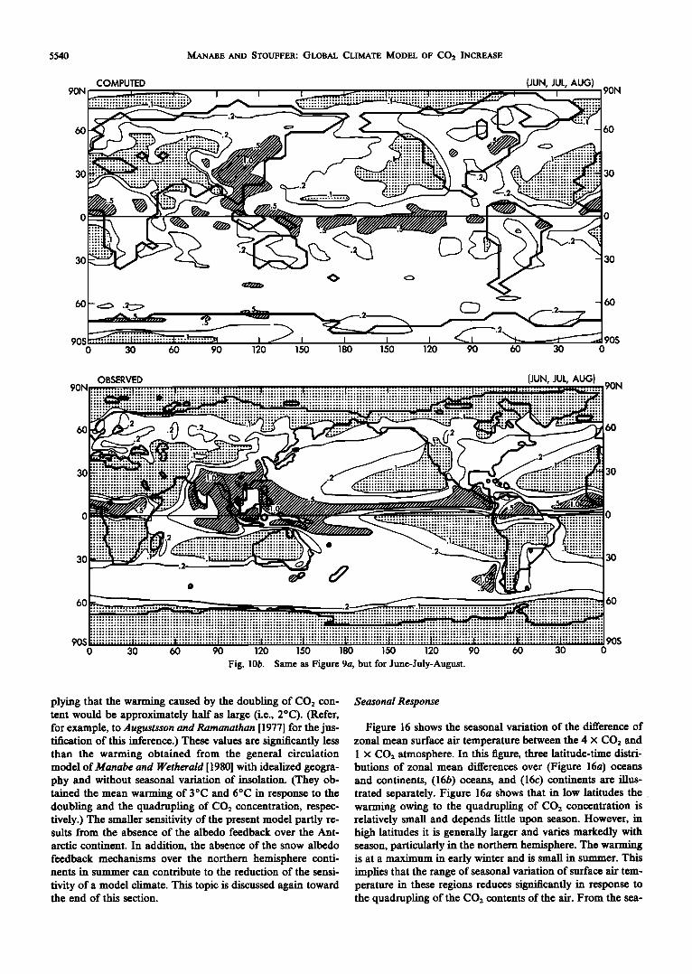
Fig. 10b. Same as Figure 9a, but for June-July-August.
3O
3O
6O
90S 0
plying that the warming caused by the doubling of CO2 con- tent would be approximately half as large (i.e., 2øC). (Refer, for example, to Augustsson and Ramanathan [1977] for the jus- tiffcation of this inference.) These values are significantly less than the warming obtained from the general circulation model of Manabe and Wetheraid [1980] with idealized geogra- phy and without seasonal variation of insolation. (They ob- tained the mean warming of 3øC and 6øC in response to the doubling and the quadrupling of CO2 concentration, respec- tively.) The smaller sensitivity of the present model partly re- suits from the absence of the albedo feedback over the Ant-
arctic continent. In addition, the absence of the snow albedo feedback mechanisms over the northern hemisphere conti- nents in summer can contribute to the reduction of the sensi-
tivity of a model climate. This topic is discussed again toward the end of this section.
Seasonal Response
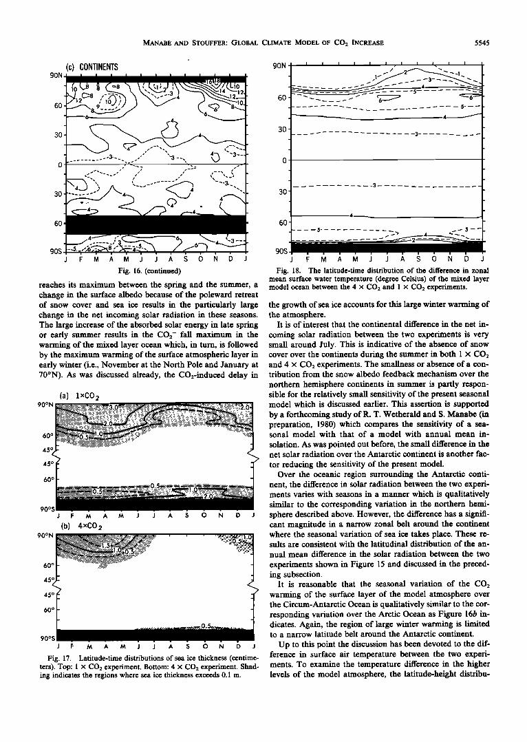
Figure 16 shows the seasonal variation of the difference of zonal mean surface air temperature between the 4 x CO2 and 1 x CO2 atmosphere. In this figure, three latitude-time distri- butions of zonal mean differences over (Figure 16a) oceans and continents, (16b) oceans, and (16c) continents are illus- trated separately. Figure 16a shows that in low latitudes the warming owing to the quadrupling of CO2 concentration is relatively small and depends little upon season. However, in high latitudes it is generally larger and varies markedly with season, particularly in the northern hemisphere. The warming is at a maximum in early winter and is small in summer. This implies that the range of seasonal variation of surface air tem- perature in these regions reduces significantly in response to the quadrupling of the CO2 contents of the air. From the sea-
MANABE AND STOUFFER: GLOBAL CLIMATE MODEL OF CO 2 INCREASE 5541
,18C
eeee
0
NORTH AMERICA
AUGUST
(c)
.0 o
9(•øE
60 ø
AUSTRALIA
NEW ZEALAND
SOUTH AM ERICA FEBRUARY / • 90,•W
(cm) 9•øE AFRICA
eeeeeeeee
ß ß
ANTARCTICA
eeeeeeeeee
SOUTH AMERICA )øW
60 ø
Fig. 11. Geographical distributions of sea ice thickness (meters) from the I x CO2 experiment. (a) Northern hemi- sphere-February. (b) Northern hemisphere--August. (c) Southern hemisphere--February. (d) Southern hemisphere-- August. Dashed-dotted lines indicate the observed mean sea ice boundaries from the compilation by U.S. Naval Oceano- graphic Office [ 1957, 1958].
NEW ZEALAND
•)o.
AUGUST
sonal variations of the zonal mean sea ice thickness shown in
Figure 17, it is observed that the sea ice from the 4 x CO,• ex- periment is everywhere less than the sea ice from the 1 x CO,• experiment. Therefore it is reasonable that the 1 x CO,• atmo- sphere is insulated by thicker sea ice from the influence of the underlying sea water so that it has a more continental climate with a larger seasonal variation of temperature than the 4 x CO,• atmosphere. Although the poleward retreat of highly re- flective snow cover and sea ice is mainly responsible for the large annual mean warming in high latitudes, the change of the thermal insulation effect of sea ice strongly influences the seasonal variation of the warming over the polar regions as is discussed below.
Figure 18 shows the seasonal variation of the zonal mean difference in surface water temperature of the mixed layer ocean model between the 4 x CO,• and I x CO,• experiment. According to the comparison between this figure and Figure 16b, the seasonal variation of the CO,• warming of the mixed layer ocean in high latitudes differs from and is much less than the variation of the warming of overlying air. This result suggests that the magnitude of the thermal insulation effect of
sea ice is highly variable with respect to season, and it de- serves further examination.
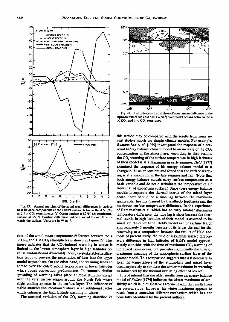
To comprehend the seasonal variation of air temperature over the Arctic Ocean, it is necessary to analyze the heat bal- ance at the underlying ocean surface. Figure 19a shows how the zonal mean differences of various surface heat balance
components (at 82øN) between the two experiments changes with respect to seasons. The surface heat balance components contained in this analysis are net solar radiation, net terres- trial radiation, sensible heat flux, latent heat flux, and oceanic heat flux. In Figure 19 a positive value indicates a heat gain for the ocean surface which results from the CO,• increase. Therefore the increases in the upward fluxes of sensible heat, latent heat, and net terrestrial radiation indicate negative con- tributions, whereas the increases in the upward oceanic heat flux and net downward solar radiation are shown to be posi- tive contributions to the surface heat balance. (Here the oce- anic heat flux includes the heat exchanges with not only the mixed layer ocean but also the sea ice. Over the ice-free re- gion, the oceanic heat flux is the heat supply from the interior to the surface of the ocean. Over the ice-free region, the oce-
5542 MANABE AND STOUFFER: GLOBAL CLIMATE MODEL OF CO2 INCREASE
o
0.25 o
o
eøøw FEBRUARY eøøw AUGUST Fig. 12. Geographical distributions of snow depth in water equivalent units (centimeters) from the I x CO2 experi-
ment. Left: February distribution. Right: August distribution. Dashed-dotted line indicates observed monthly mean snow margin from Wiesnet and Matson [1979].
anic heat flux is the heat supply from the interior to the sur- face of the ocean. Over the ice covered region it is the upward conductive heat flux through ice minus the rate of latent heat consumption owing to the melting of the upper ice surface.)
Figure 19a indicates that in summer, the absorption of solar radiation by the Arctic Ocean surface in the 4 x CO2 experi- ment is much larger than the corresponding absorption in the 1 x CO2 experiment. This difference results from the reduc- tion of surface albedo caused by the disappearance of sea ice or the formation of water puddles over the sea ice. The figure also indicates the net gain of terrestrial radiation energy by the Arctic Ocean surface during summer in the 4 x CO2 ex- periment in comparison with the 1 x CO2 experiment. This additional energy of both solar and terrestrial radiation is transferred directly into downward oceanic heat flux as is in- dicated by Figure 19a, and it enhances the melting of sea ice and increases the warming of mixed layer ocean as revealed by Figure 18. Accordingly, the additional radiation energy does not contribute to the warming of the model atmosphere. (Instead, downward fluxes of sensible and latent heat further removes the heat from the atmosphere as implied by small gain of sensible and latent heat by the ocean surface in sum- mer.) Thus the CO2 warming of the surface layer of the atmo- sphere over the Arctic Ocean is relatively small as Figure 16b indicates. However, it is expected, that the additional heat re- ceived by the mixed layer sea ice system delays the formation of the sea ice or reduces its thickness. This results in the re-
duction of the thermal insulation effect of the sea ice in early winter, when the air-sea temperature difference becomes large and enhances the warming of the surface atmospheric layer.
This reduction in the thermal insulation effect of the sea ice
is indicated in Figure 19a as a large positive difference in the
oceanic heat flux around November. (As defined earlier, oce- anic heat flux includes heat conduction through the sea ice.) This change in the oceanic heat flux is accompanied by a large early winter increase in the sensible and latent heat fluxes into the atmosphere. (Note, in Figure 19a, a large negative differ- ence in the sensible heat flux around November.) Thus the CO2-induced warming in the surface layer of the atmosphere is most pronounced in early winter.
As the winter season proceeds, sea ice in both the 1 x CO2 and 4 x CO2 experiments becomes sufficiently thick that the difference in upward conductive heat flux becomes relatively small. Thus the magnitude of the CO2-induced warming of surface air (through sensible heat flux) in late winter is less than that of early winter. Meanwhile, the warming of the mixed layer temperature is very close to zero as the temper- ature of water beneath sea ice is assumed to remain at the
freezing point (i.e., -2øC). According to Figure 16b the time of maximum warming of
the surface layer of the atmosphere becomes later with de- creasing latitude. (For example, at 70øN, the warming is at a maximum in January rather than early winter when maxi- mum warming occurs near the North Pole.) This result is con- sistent with the fact that the time of sea ice formation in both
experiments becomes later with decreasing latitudes as in- dicated in Figure 17.
Figure 20 illustrates the latitude-time distribution of zonal mean difference in the upward flux of sensible heat between the 4 x CO2 and 1 x CO2 experiments. (Note that in this fig- ure, the sign of sensible heat flux difference is reversed from Figure 19a). Again, this figure indicates the reduction of up- ward sensible heat flux in summer and the increase in the late
fall and winter in response to the increase of CO2 concentra-
MANABE AND STOUFFER: GLOBAL CLIMATE MODEL OF CO2 INCREASE 5543
1 oo I I
75 •,. (a)NET 50
25
-25
-50
-75
-lOO
350
325'
3OO
275
NORTHERN HEMISPHERE :
[ [ [ [ ] •.••1 ........
NORTHERN HEMISPHERE ?" + ._:.
xx r .-"' + \ / -
% ..-' • .f+ -
I I
• (b)SOLAR
_
ß
\ • \ : \ I \ . 250 ß I ..'
2 ß '\ ø ø 225 --
/ • GLOBAL ...' ]q 200 -- / -p: / X --
ß X
• •... .... .•-' 150 - ' ....... • •sP• • • +
•25, i I , I i I I I I , I I I
2751 I I I I I I I '1 I I I I I •c) TERRESTRIAL __ _ •o•• •sP•g•l
250 F ................... x •• .... , •2 '"•-.•, x x .• ......... •' 225• • • + + • • --•
2oo• • I I I I I I I I I I / 3 F M A M 3 3 A S O N D •
MONTH
Fig. 13. Seasonal variation of hemispheric and global mean values of radiative fluxes at the top of the atmosphere. Top: net radiative flux (net downward solar flux minus upward terrestrial flux); middle: net downward solar flux (incoming solar flux minus reflected radiation); bottom: upward terrestrial flux. Units are W m -2. Observed fluxes are deduced from satellite observations by Ellis and Vonder Haar [1976]. They are indicated by crosses (northern hemisphere), pluses (south- ern hemisphere), and dots (global domain).
• ..... ••."• :::::-. i iiii::::iiii:i 7.-3 ...... ,..... :::: :0 "• • • ii ! i i ! i ! i i :: :: :: :: :: :..:: :•-'"••-• •____, ...... :-"-'• --:.:•.::i:: • 205 n-
if) • ....... .......... :• .-..... :.:+:..'• ::........:...........:..........:.....•• "' 3so :::::::::::::::::::::::::::::::::::::::::::::::::::::: iii x m 515 5
940.1¾ 'o .... ' "'-' ' '" • '" '"' '•'"•-.N:" .'•::•.' .." '.".."..' : l •'• • ========================== •:.:.',' 990 o o o o o o o 90 N 60 30 0 30 60 90 S
Fig. 14. Latitude height distribution of the zonal mean difference in annual mean temperature (degrees Kelvin) of the model atmosphere between the 4 x CO2 and I x CO2 experiment.
5544 MANABE AND STOUFFER: GLOBAL CLIMATE MODEL OF CO 2 INCREASE
•2
0 I I I I I 90øN 60 ø 30 ø 0 30 ø 60 ø 90øS
LATITUDE
Fig. 15. Latitudinal distribution of the zonal mean difference in the annual mean net incoming solar radiation at the top of the model atmosphere between the 4 x CO2 and I x CO2 experiment.
tion. It is significant that the time of maximum increase be- comes later with decreasing latitude and accounts for the phase variation in the latitude-time distribution of air temper- ature difference as discussed above.
The seasonal variation of the difference in the surface air
temperature between the two experiments over the model continents is significantly different from the variation over the model oceans. According to Figure 16c, which shows the lati- tude-time distribution of the difference in zonal mean surface
air temperature over continents, the CO2 warming in high lati- tudes is at a maximum in early winter is being influenced by the large warming over the Arctic Ocean discussed above. However, the figure also indicates a secondary center of rela-
30 tively large warming around 65øN in April. To determine the mechanism for this spring maximum, the seasonal variation of zonal mean differences of the continental heat balance com-
60 ponents (at 65øN) between the two experiments are illustrated in Figure 19b in the same manner as Figure 19a. This figure indicates the large spring maximum in the difference of net 90S downward solar radiation between the two experiments. Since the incoming solar radiation of late spring is large in high lati- tudes, the reduction of highly reflective snow covered area in spring causes a large increase in the amount of solar radiation absorbed by the continental surface. This additional solar en- ergy immediately raises the temperature of continental surface and is responsible for the increase in the upward fluxes of both sensible and latent heat into the model atmosphere as in- dicated in Figure 19b by the large negative differences of these fluxes around May. (Note that the heat capacity of continen- tal surface is assumed to be zero.) Thus the aforementioned spring maximufia in warming occurs.
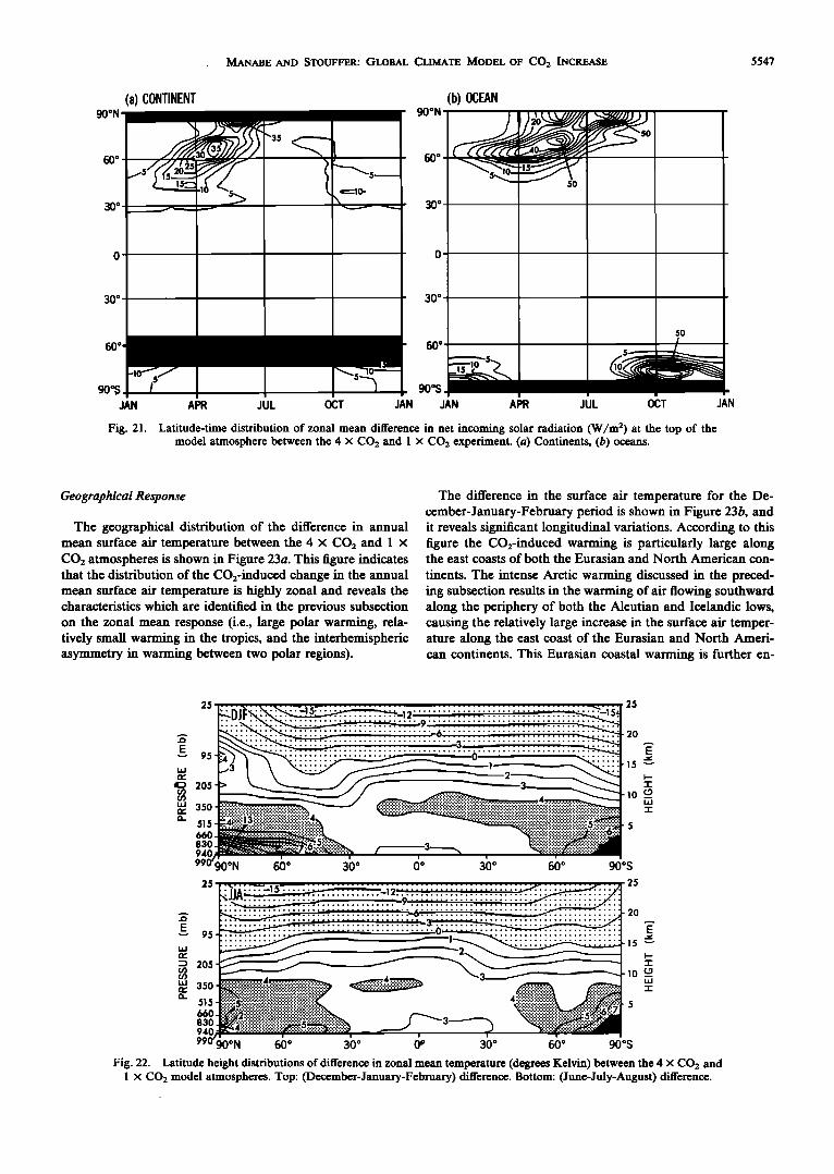
It is important to recognize here that the influence of the al- bedo feedback mechanism upon the change in net incoming solar radiation is pronounced in the spring or early summer over the oceans as well as over the continents. This is evident 30 in Figure 21, which shows the latitude-time distribution of the zonal mean difference in net incoming solar radiation at the top of the atmosphere between the 4 x CO• and 1 x CO• ex- 60 periments. The zonal mean difference is shown separately for continental and oceanic regions. According to this figure the increase in the net incoming solar radiation over continents is most pronounced in March at around 50øN, in May at around 70øN, and in June near the North Pole. Over oceans the in- crease is most pronounced in the beginning of May at about 70øN and in August near the North Pole. Since the high lati- tude insolation has pronounced seasonal variation and
(a) OCEANS AND CONTINENTS 90N • , • • •. • , ' .....
,,/'.J; ", il '1/,:/"' ',-,..' , \ 2J ,' \ • / I ', • .-' ) '"'-•,,]o.L-'
60 : ......... •- 6 '"-' " •6
-...... • ......... .. 3_ _- .-•... s •-
4 '"- 6 '• 4
J F M A M J J A S 0 N D J
(b) OCEANS
6o
30-
.
o
9OS J F M A M J J A S O N D J
Fig. 16. Latitude-time distribution of zonal mean difference in surface air temperature (degrees Kelvin) between the 4 x CO2 and 1 x CO2 experiment. (a) Oceans and continents, (b) oceans, and (c) continents. The difference is computed at the lowest finite difference level located at about 70 m above the earth's surface.
MANABE AND STOUFFER.' GLOBAL CLIMATE MODEL OF CO 2 INCREASE 5545
90N (c) CONTINENTS
6o
30
6O
90S J F M A M J J A S 0 N D J
Fig. 16. (continued)
reaches its maximum between the spring and the summer, a change in the surface albedo because of the poleward retreat of snow cover and sea ice results in the particularly large change in the net incoming solar radiation in these seasons. The large increase of the absorbed solar energy in late spring or early summer results in the CO:- fall maximum in the warming of the mixed layer ocean which, in turn, is followed by the maximum warming of the surface atmospheric layer in early winter (i.e., November at the North Pole and January at 70øN). As was discussed already, the CO2-induced delay in
(a) lxCO 2
u r .......... "•••'":•::'•'.'••.•:".":•ii:.::.•ii!:•:::::: !i:• ......
45ø f 60 ø [-
90øS J F M A M J J A S O N D J
(b) 4xCO 2 90øN -,r-.••-.•-..•.••.•..••••••••••:.....•::•::..:.•.•.•,=.....•.. •......• ........•••:•:.:..:.:.:.:;.s..:•.:: , , ' """"•" '•':' ' ':' •"•' ß '•. ß ß - ß ' '. ß .- ß :•••.'.'.1 0
"- '" '- '" .............
60ø • ...................... .":' ...... "' ':'•.' :.'-";:: • ............
45ø f 60ø I
90os
J F M A M J J A S O N D J
Fig. 17. Latitude-time distributions of sea ice thickness (centime- ters). Top: I x CO2 experiment. Bottom: 4 x CO2 experiment. Shad- ing indicates the regions where sea ice thickness exceeds 0.1 m.
90N
60
30
30
60
90S •- J F M A M J J A S 0 N D J
Fig. 18. The latitude-time distribution of the difference in zonal mean surface water temperature (degree Celsius) of the mixed layer model ocean between the 4 x CO2 and I x CO2 experiments.
the growth of sea ice accounts for this large winter warming of the atmosphere.
It is of interest that the continental difference in the net in-
coming solar radiation between the two experiments is very small around July. This is indicative of the absence of snow cover over the continents during the summer in both 1 x CO• and 4 x CO: experiments. The smallness or absence of a con- tribution from the snow albedo feedback mechanism over the
northern hemisphere continents in summer is partly respon- sible for the relatively small sensitivity of the present seasonal model which is discussed earlier. This assertion is supported by a forthcoming study of R. T. Wetheraid and S. Manabe (in preparation, 1980) which compares the sensitivity of a sea- sonal model with that of a model with annual mean in-
solation. As was pointed out before, the small difference in the net solar radiation over the Antarctic continent is another fac-
tor reducing the sensitivity of the present model. Over the oceanic region surrounding the Antarctic conti-
nent, the difference in solar radiation between the two experi- ments varies with seasons in a manner which is qualitatively similar to the corresponding variation in the northern hemi- sphere described above. However, the difference has a signifi- cant magnitude in a narrow zonal belt around the continent where the seasonal variation of sea ice takes place. These re- sults are consistent with the latitudinal distribution of the an- nual mean difference in the solar radiation between the two
experiments shown in Figure 15 and discussed in the preced- ing subsection.
It is reasonable that the seasonal variation of the CO,• warming of the surface layer of the model atmosphere over the Circum-Antarctic Ocean is qualitatively similar to the cor- responding variation over the Arctic Ocean as Figure 16b in- dicates. Again, the region of large winter warming is limited to a narrow latitude belt around the Antarctic continent.
Up to this point the discussion has been devoted to the dif- ference in surface air temperature between the two experi- ments. To examine the temperature difference in the higher levels of the model atmosphere, the latitude-height distribu-
5546 MANABE AND STOUFFER.' GLOBAL CLIMATE MODEL OF CO2 INCREASE
w
90øN I I I I I I I 80 j I 1(82N ) I (a) Ocean
70 ........... SENSIBLE HEAT FLUX
..... LATENT HEAT FLUX
60 ...... NET TERRESTRIAL RADIATION .... NET SOLAR RADIATION
50 OCEAN HEAT FLUX I I 40 I
I I 30 I
I I 20 I
lO
-20 ß
ß
.
-30
-40 \'""...../ -50
-60
-70
-80 I I I
50 I • i (b) Continents (65N)
i i I
! I i I i i I
•" SNOW MELT
3o- / ', I % -
I 20- I
/ \ - W In - /
I• .,./ _ %..,"'" ..... ',,, •,•
I "--• / • •--•'• -- %...
,'-.,, '•.• /./' -301 I I I I' I • I I I I /
J F M A M J J A S O N D
TIME (month)
Fig. 19. Annual marches of the zonal mean differences in various heat balance components at the earth's surface between the 4 x CO2 and I x CO2 experiments. (a) Ocean surface at 82øN, (b) continental surface at 65øN. Positive difference indicate an additional flux to- wards the surface. Units are in W m -•.
tion of the zonal mean temperature difference between the 4 x CO• and 1 x CO• atmospheres is shown in Figure 22. This figure indicates that the CO•-induced warming in winter is limited to the lowest atmosphere layer in high latitudes be- cause,asManabeand Wetheraid[ 1975 ] suggested, stable stratifica- .tion tends to prevent the penetration of heat into the upper model troposphere. On the other hand, the warming tends to spread over the entire model troposphere in lower latitudes where moist convection predominates. In summer, similar spreading of warming takes place at most latitudes except over the very narrow region around the North Pole where
60 ø
30 ø
o
30 ø
60 ø-
90øS
JAN APR JUL OCT JAN
Fig. 20. Latitude-time distribution of zonal mean difference in the upward flux of sensible heat (W/m 2) over model oceans between the 4 x CO2 and I x CO2 experiment.
this section may be compared with the results from some re- cent studies which use simple climate models. For example, Rarnanathan et al. [1979] investigated the response of a sea- sonal energy balance climate model to an increase of the CO• concentration in the atmosphere. According to their results, the CO• warming of the surface temperature in high latitudes of their model is at a maximum in early summer. Held [1977] examined the response of his energy balance model to a change in the solar constant and found that the surface warm- ing is at a maximum in the late summer and fall. (Note that both energy balance models carry surface temperature as a basic variable and do not discriminate the temperature of air from that of underlying surface.) Since these energy balance models incorporate the thermal inertia of the mixed layer ocean, there should be a time lag between the maximum spring solar heating (caused by the albedo feedback) and the maximum surface temperature difference. In the experiment of Ramanathan et al. which has an early summer maximum temperature difference, the time lag is short because the ther- mal inertia in high latitudes of their model is assumed to be small. On the other hand, Held's model exhibits a time lag of approximately 3 months because of its larger thermal inertia. According to a comparison between the results of Held and those of present study, the time of maximum surface temper- ature difference in high latitudes of Held's model approxi- mately coincides with the time of maximum CO• warming of the mixed layer ocean, but precedes significantly the time of maximum warming of the atmospheric surface layer of the present model. This comparison suggests that it is necessary to treat the temperatures of the atmosphere and mixed layer ocean separately to simulate the winter maximum in warming as influenced by the thermal insulating effect of sea ice.
It is of interest that the older results from an energy balance model of Sellers [1974] indicates the winter maximum of sen-
slight cooling appears in the surface layer. The influence of sitivity which is in qualitative agreement with the results from stable stratification mentioned above is an additional factor the present study. However, his winter maximum appears to which enhances the high latitude warming in winter. result from a somewhat different mechanism which has not
The seasonal variation of the CO2 warming described in been fully identified by the present authors.
MANABE AND STOUFFER.' GLOBAL CLIMATE MODEL OF CO 2 INCREASE 5547
90øN
0
(a) CONTINENT (b) OCEAN
• • •s '"'-' s• so
50
90ø$ . JAN APR JUL OCT JAN JAN APR JUL OCT JAN
Fig. 21. Latitude-time distribution of zonal mean difference in net incoming solar radiation (W/m 2) at the top of the model atmosphere between the 4 x CO2 and 1 x CO2 experiment. (a) Continents, (b) oceans.
Geographical Response
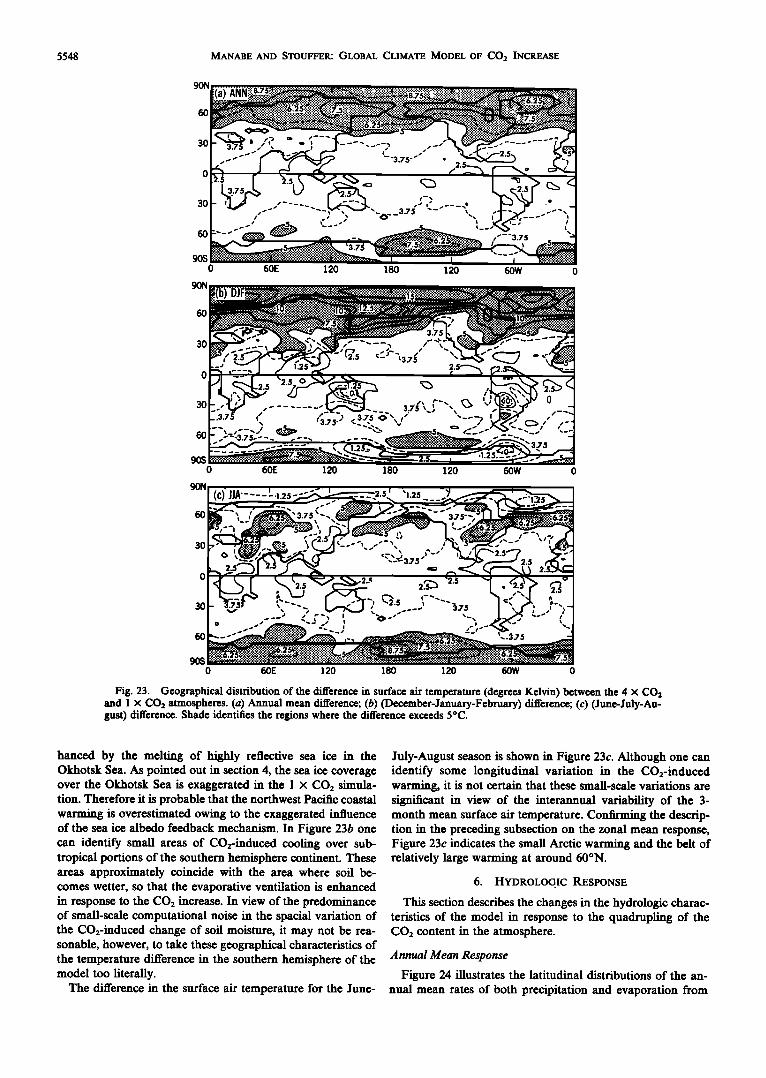
The geographical distribution of the difference in annual mean surface air temperature between the 4 x CO2 and I x CO2 atmospheres is shown in Figure 23a. This figure indicates that the distribution of the CO2-induced change in the annual mean surface air temperature is highly zonal and reveals the characteristics which are identified in the previous subsection on the zonal mean response (i.e., large polar warming, rela- tively small warming in the tropics, and the interhemispheric asymmetry in warming between two polar regions).
The difference in the surface air temperature for the De- cember-January-February period is shown in Figure 23b, and it reveals significant longitudinal variations. According to this figure the CO:-induced warming is particularly large along the east coasts of both the Eurasian and North American con-
tinents. The intense Arctic warming discussed in the preced- ing subsection results in the warming of air flowing southward along the periphery of both the Aleutian and Icelandic lows, causing the relatively large increase in the surface air temper- ature along the east coast of the Eurasian and North Ameri- can continents. This Eurasian coastal warming is further en-
25 25
..-. '•,-6 ............................... 20
E 9,5 ............................ :::'•;:::::• ................ E u.J 1 15 "-' n- 2 I--
• 205 -r- u') lO c9 cu 350
515 ...:.:.:.: .......... 5 660 830
T
90øN 60 ø 30 ø 0 ø 30 ø 60 ø 90øS
25 25
•.• . 20 • 1,5 "-' g
O0 U :" "":" 2:':':':':':':':':':':':':':':':':':':':':':':':':':':" '"':':':':':':':':':':':':':':':':': ',,• •":':g ':•'•
:.:.:.' ..:.:.:.'.'.....:.:-'
9 4 0 ':':':':':':':':':':':':':" '":':':'"":':':':':' ":':':':':" o o o 99•90øN 60 ø 30 ø 0 •' 30 60 90 S Fig. 22. Latitude height distributions of difference in zonal mean temperature (degrees Kelvin) between the 4 x CO2 and
1 x CO2 model atmospheres. Top: (December-January-February) difference. Bottom: (June-July-August) difference.
5548 MANABE AND STOUFFER: GLOBAL CLIMATE MODEL OF C02 INCREASE
90N
60
30
30
I•(a) ANN::•..%-r.•'"'"'••:':••.•: ....... :,!,•i..•i:.•.'•,:•:.a:,::'•:As.7:::::::::::::::::::::::: :i:5 ....... :.::.:...::.. •:!:• ..... '"-..:.'..':.:::..'/;:: "'•;....' .'...-• '":':':'" '" "•• ii• iii:.':.::'/.'. • •-• '-' •-'"'•i! i' '""" -'.......' ."• "..•'"-'-'-'••
-'•. ' : • ' -i - - •- -•' .... '" -'"'"" ' " "• .........
....,... , .. '"' "-,-".,.,,..."-'._ ..:: _
, ..- . ;' :: -- •.,• ,, •_• ---• [.....-- .•g.:.• ---. •.•..&.:.:...• .... • [---' .:_ ...'::• '"'"'-• ,• ,.-, ,•"'""*:•.":'":•:••••'.•....:::•• /--'3.75 • -' ß ':;:;:::;: •' ; 7 5 ::::::::::'; ..•...a•. ! ß 5 ..:.:.:.:.:.:.:.. 3.75 '.'•,.'....'.?;:;::•_•.. .............. :'.".": .... • ...... ... ======================= • •:""- :.. ;•:...........'•-•:•..."'"'"'•"'''"' "-••••" ':":"'• :_•i:::':-::.--/...'.:• • ' ' '" ' ' ' ' '"'"'"'"'"'"'"•' ß ß ß '"'""•'"'..•:::::::::::'"'"':':. ß ß. :"::- - - -:;:::::::::;:;:"::::•'"'•:".'::- -. -":-':-'::..'.;.-'.• I .... I •
60E 120 180 120 60W 0 90S
0
90N
60
30
30
0 60E 120 180 120 60W 0
Fig. 23. Geographical distribution of the difference in surface air temperature (degrees Kelvin) between the 4 X CO2 and 1 x CO2 atmospheres. (a) Annual mean difference; (b) (December-January-February) difference; (c) (June-July-Au- gust) difference. Shade identifies the regions where the difference exceeds 5øC.
hanced by the melting of highly reflective sea ice in the Okhotsk Sea. As pointed out in section 4, the sea ice coverage over the Okhotsk Sea is exaggerated in the 1 x CO2 simula- tion. Therefore it is probable that the northwest Pacific coastal warming is overestimated owing to the exaggerated influence of the sea ice albedo feedback mechanism. In Figure 23b one can identify small areas of CO2-induced cooling over sub- tropical portions of the southern hemisphere continent. These areas approximately coincide with the area where soil be- comes wetter, so that the evaporative ventilation is enhanced in response to the CO2 increase. In view of the predominance of small-scale computational noise in the spacial variation of the CO2-induced change of soil moisture, it may not be rea- sonable, however, to take these geographical characteristics of the temperature difference in the southern hemisphere of the model too literally.
The difference in the surface air temperature for the June-
July-August season is shown in Figure 23c. Although one can identify some longitudinal variation in the CO:-induced warming, it is not certain that these small-scale variations are significant in view of the interannual variability of the 3- month mean surface air temperature. Confirming the descrip- tion in the preceding subsection on the zonal mean response, Figure 23c indicates the small Arctic warming and the belt of relatively large warming at around 60øN.
6. HYDROLOGIC RESPONSE
This section describes the changes in the hydrologic charac- teristics of the model in response to the quadrupling of the CO: content in the atmosphere.
Annual Mean Response
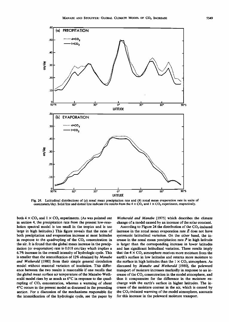
Figure 24 illustrates the latitudinal distributions of the an- nual mean rates of both precipitation and evaporation from
MANABE AND STOUFFER: GLOBAL CLIMATE MODEL OF CO2 INCREASE 5549
.eoj (a) PREC•i[•TION 50 ......... 2 "
.40
.:30
.20
.10
0
90øN 60 ø 30 ø 0 ø 30 ø 60 ø 90øS
LATITUDE
.6O
(b) EVAPORATION
.50 - ' ........ 4xC02 -
lxCO 2
.40 -
• .:30
.20
.10
0 I I I I I 90øN 60 ø 30 ø 0 ø 30 ø 60 ø 9005
LATITUDE
Fig. 24. Latitudinal distributions of (a) zonal mean precipitation rate and (b) zonal mean evaporation rate in units of centimeters/day. Solid line and dotted line indicate the results from the 4 x CO2 and I x CO2 experiment, respectively.
both 4 x CO2 and 1 x CO2 experiments. (As was pointed out in section 4, the precipitation rate from the present low-reso- lution spectral model is too small in the tropics and is too large in high latitudes.) This figure reveals that the rates of both precipitation and evaporation increase at most latitudes in response to the quadrupling of the CO•_ concentration in the air. It is found that the global mean increase in the precip- itation (or evaporation) rate is 0.018 cm/day which implies a 6.7% increase in the overall intensity of hydrologic cycle. This is smaller than the intensification of 12% obtained by Manabe and Wetheraid [1980] from their simple general circulation model without seasonal variation of insolation. This differ-
ence between the two results is reasonable if one recalls that
the global mean surface air temperature of the Manabe-Weth- erald model rises by as much as 6øC in response to the quad- rupling of CO•_ concentration, whereas a warming of about 4øC occurs in the present model as discussed in the preceding section. For a discussion of the mechanisms responsible for the intensification of the hydrologic cycle, see the paper by
Wetherald and Manabe [1975] which describes the climate change of a model caused by an increase of the solar constant.
According to Figure 24 the distribution of the CO•_-induced increase in the zonal mean evaporation rate/• does not have systematic latitudinal variation. On the other hand, the in- crease in the zonal mean precipitation rate/5 in high latitude is larger than the corresponding increase in lower latitudes and has significant latitudinal variation. These results imply that the 4 x CO•_ atmosphere receives more moisture from the earth's surface in low latitudes and returns more moisture to
the surface in high latitudes than the 1 x CO•_ atmosphere. As discussed by Manabe and Wetherald [1980], the poleward transport of moisture increases markedly in response to an in- crease of the CO•_ concentration in the model atmosphere, and thus it compensates for the difference in the moisture ex- change with the earth's surface in higher latitudes. The in- crease of the moisture content in the air, which is caused by the CO•_-induced warming of the model atmosphere, accounts for this increase in the poleward moisture transport.
5550 MANABE AND STOUFFER: GLOBAL CLIMATE MODEL OF CO2 INCREASE
.O6
.O5
.O4
.O3
.02
.Ol
o
:Ol
-.02
-.03
.04
.03
ø02
>, .01 o
• 0 E u -.01
-.02
-.O3
-.04
-.05 90N
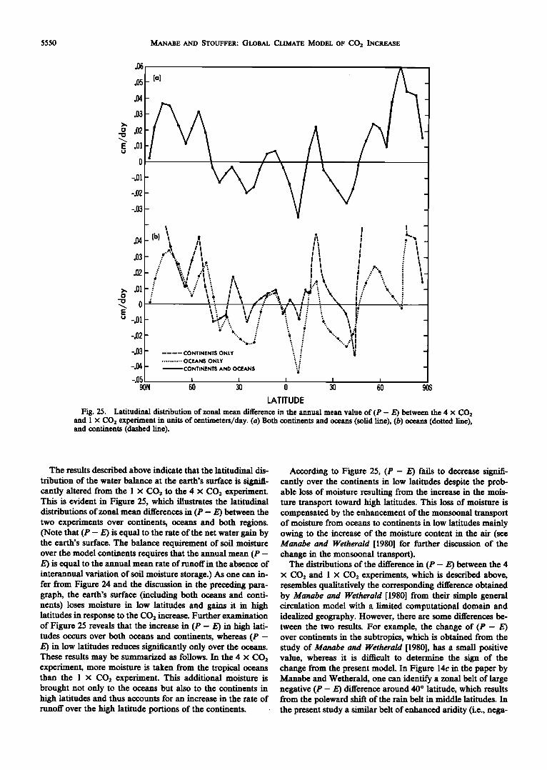
(b) %
' L •," .),
- ". '•'.• .•
- -------- CONTINENTS ONLY ........... OCEANS ONLY
- CONTINENTS AND OCEANS I I I I I
60 30 0 30 60
LATITUDE
ß i
90S
Fig. 25. Latitudinal distribution of zonal mean difference in the annual mean value of (P - E) between the 4 x CO2 and I x CO2 experiment in units of centimeters/day. (a) Both continents and oceans (solid line), (b) oceans (dotted line), and continents (dashed line).
The results described above indicate that the latitudinal dis-
tribution of the water balance at the earth's surface is signifi- cantly altered from the 1 x CO2 to the 4 x CO2 experiment. This is evident in Figure 25, which illustrates the latitudinal distributions of zonal mean differences in (P - E) between the two experiments over continents, oceans and both regions. (Note that (P - E) is equal to the rate of the net water gain by the earth's surface. The balance requirement of soil moisture over the model continents requires that the annual mean (P - E) is equal to the annual mean rate of runoff in the absence of interannual variation of soil moisture storage.) As one can in- fer from Figure 24 and the discussion in the preceding para- graph, the earth's surface (including both oceans and conti- nents) loses moisture in low latitudes and gains it in high latitudes in response to the CO2 increase. Further examination of Figure 25 reveals that the increase in (P - E) in high lati- tudes occurs over both oceans and continents, whereas (P - E) in low latitudes reduces significantly only over the oceans. These results may be summarized as follows. In the 4 x CO2 experiment, more moisture is taken from the tropical oceans than the 1 x CO2 experiment. This additional moisture is brought not only to the oceans but also to the continents in high latitudes and thus accounts for an increase in the rate of runoff over the high latitude portions of the continents.
According to Figure 25, (P - E) fails to decrease signifi- cantly over the continents in low latitudes despite the prob- able loss of moisture resulting from the increase in the mois- ture transport toward high latitudes. This loss of moisture is compensated by the enhancement of the monsoonal transport of moisture from oceans to continents in low latitudes mainly owing to the increase of the moisture content in the air (see Manabe and Wetheraid [1980] for further discussion of the change in the monsoonal transport).
The distributions of the difference in (P - E) between the 4 x CO2 and 1 x CO2 experiments, which is described above, resembles qualitatively the corresponding difference obtained by Manabe and Wetheraid [1980] from their simple general circulation model with a limited computational domain and idealized geography. However, there are some differences be- tween the two results. For example, the change of (P - E) over continents in the subtropics, which is obtained from the study of Manabe and Wetheraid [1980], has a small positive value, whereas it is difficult to determine the sign of the change from the present model. In Figure 14c in the paper by Manabe and Wetheraid, one can identify a zonal belt of large negative (P- E) difference around 40 ø latitude, which results from the poleward shift of the rain belt in middle latitudes. In the present study a similar belt of enhanced aridity (i.e., nega-
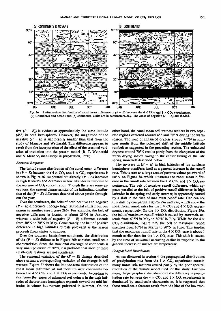
MANABE AND STOUFFER: GLOBAL CLIMATE MODEL OF CO 2 INCREASE 5551
90øN
60 ø
•0 ø
30 ø
60 ø
(a) CONTINENTS & OCEANS (b) CONTINENTS
" ß . .... ß • .. .• • ....
•'.-.'.'.'-'•e'"•N'""" ß ß -•-'"-'• •-'• •-'-'"n ß -,:.- •.:::: :.:.:.:.:.:.•: '.•.'.', '.:•:• w+•.:.:.:.:.' ß. -.-.:.:.•.• '"'¾• . :. :. :. :. :.: •:..•:::. k•---- •-• •-:.:-:-:-:-:-:-:-:-•5 .'•..
.....
...... • •,..-.-........................
.:.:.:.•.. z....•.:....:.:c..•::.:.•:.:.•:•:•':':':'¾c••' •:::. :.:.:•:•.•.:.:..:,•.••:• --•'•'•:•::•: ::•::'$?•:•:.•.:.:.::::• . .•...v ..-•• ß .........
.• , _• . , .••"• .... • --- .... •.. • •
.... .025 90øS
JAN APR JUL OCT JAN JAN APR JUL OCT JAN
Fig. 26. Latitude-time distribution of zonal mean difference in (P - E) between the 4 x CO2 and I x CO2 experiments. (a) Continents and oceans and (b) continents. Units are in centimeters/day. The areas of negative (P - E) are shaded.
tive (P - E)) is evident at approximately the same latitude (45 ø ) in both hemispheres. However, the magnitude of the negative (P - E) is significantly smaller than that from the study of Manabe and Wetheraid. This difference appears to result from the incorporation of the effect of the seasonal vari- ation of insolation into the present model (R. T. Wetheraid and S. Manabe, manuscript in preparation, 1980).
Seasonal Response
The latitude-time distribution of the zonal mean difference
in (P - E) between the 4 x CO2 and 1 x CO2 experiments is shown in Figure 26. As pointed out already, (P - E) increases in high latitudes and decreases in low latitudes in response to the increase of CO2 concentration. Though there are some ex- ceptions, the general characteristics of the latitudinal distribu- tion of the (P- E) difference described above persist through- out the year.
Over the continents, the belts of both positive and negative (P- E) differences undergo large latitudinal shifts from one season to another (see Figure 26b). For example, the belt of negative difference is located at about 25øN in January, whereas a wide belt of negative (P - E) difference extends from 30øN to 70øN in May. Concurrently, the belt of positive difference in high latitudes retreats poleward as the season proceeds from winter to summer.
Over the southern hemisphere continents, the distribution of the (P- E) difference in Figure 26b contains small-scale characteristics. Since the fractional coverage of continents is very small poleward of 30øS, it is probable that most of these small-scale features are not significant.
The seasonal variation of the (P- E) change described above causes a corresponding variation of the change in soil wetness. Figure 27 shows the latitude-time distribution of the zonal mean difference of soil moisture over continents be-
tween the 4 x CO2 and 1 x CO2 experiments. According to this figure the region of enhanced soil wetness in the high lati- tudes of the northern hemisphere expands toward the mid-lat- itudes in winter but retreats poleward in summer. On the
other hand, the zonal mean soil wetness reduces in two sepa- rate regions centered around 45 ø and 70øN during the warm season. The zone of enhanced dryness around 45øN in sum- mer results from the poleward shift of the middle latitude rainbelt as suggested in the preceding section. The enhanced dryness around 70øN results partly from the elongation of the warm drying season owing to the earlier timing of the late spring snowmelt described below.
The increase in (P - E) in high latitudes of the northern hemisphere manifests itself as a general increase in the runoff rate. This is seen as a large area of positive values poleward of 60øN on Figure 28, which illustrates the zonal mean differ- ence in the runoff rate between the 4 x CO2 and 1 x CO2 ex- periments. The belt of negative runoff difference, which ap- pears parallel to the belt of positive runoff difference in high latitudes in the spring and early summer, is apparently caused by a shift in the time of maximum runoff rate. One can see this shift by comparing Figures 29a and 29b, which show the zonal mean runoff rates for the 1 x CO2 and 4 x CO2 experi- ments, respectively. On the 1 x CO2 distribution, Figure 29a, the belt of maximum runoff, which is caused by snowmelt, ex- tends from 60øN in May to 80øN in July. While for the 4 x CO: distribution, Figure 29b, the belt of maximum runoff stretches from 60øN in March to 80øN in June. This implies that the maximum runoff rate in the 4 x CO: case is about 1 month earlier than for the 1 x CO: case. This shift is caused by the time of snowmelt occurring earlier in response to the general increase of surface air temperature.
Geographical Distribution
As was discussed in section 4, the geographical distributions of precipitation rate from the 1 x CO: experiment contain many unrealistic features caused partly by the poor spectral resolution of the climate model used for this study. Further- more, the geographical distribution of the difference in precip- itation rate between the 4 x CO2 and 1 x CO2 experiments is dominated by small-scale characteristics. It is suspected that these small-scale features result from the bias of the low reso-
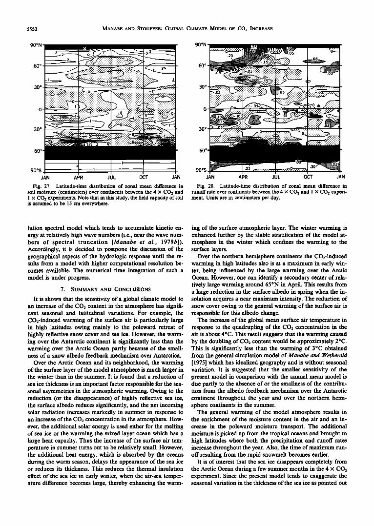
5552 MANABE AND STOUFFER: GLOBAL CLIMATE MODEL OF CO 2 INCREASE
90øN
60"
30"
30"
'"' "".....:•::i: :!::::::'i'.iiiii:iiii::::•...
- :..:.:..•::...:.:.:.: .'.:? __ ..•-•.....-:-:.:-:.:-:-•-.-.- •--•..' :• '""'"'"'"' i".'.'.'.'..'."•-0 ' '.'.'.'.'.'.'.'.'.'.'.'.'.'.'.'.-•'.'.'.'.'.'.'.'.'.', :'-'--' "•:'--•._-':!•::.:.:.:.:..:.:.:.:...'..:..'.':• •:i.•.:.:.:.:.:.:.:.:.:.:.:...' ::::: :::' :.;-:-.-Z.;:;:;:;;;:::::;-:::: ::::::::::::::::::::: '"•::':::::::::::-:: ::::;:.:" ..",./'":-•-""•.':'. ß :.;.;.:.;........ 0,._•_ ß.......................•..• .:...........:.,.........:...--.•..._.....•. ;.
- • - ,•..;.:.•--?;.:.;.;•--•. ,'"- , ),.:-;.;..',,,;• '.---....,4D,;.;.;.;-;.;.;.)'"• • ..... .'-'-'---"'.'.'".'.'-• l& ½:.'-'.'-'.'.' ,•)'.'.'-'.'-' :•0- ß '-'-' ' ' '-1' i":':':""" ' ' ' c_• -'-'-'-:.' ' -:-:.:-' ' '.:..... ß ' '•-' .. ,-.:..••• :: :-::':•';'• • %:• t..<. '•..: :..:: :..?:• ---- ' ...... "': •l• .-./77..;-:.:-:-."•:..:.;-:,'.'-.-2•0' '•----• •--• • /:-'•-:-O'----:Q_:::-:-:-:':".......'---,-m•_._
' -4•..:::::::-:.::: :'.:-i :::::::::::::::::::::: :::':•:.--'.'.--•":-•' ::. ;.: ':': :% ....., ... ...... ................ :..:.=.
1
90os - .• --
JAN APR JUL OCT JAN
Fig. 27. Latitude-time distribution of zonal mean difference in soil moisture (centimeters) over continents between the 4 x CO•_ and I x CO•_ experiments. Note that in this study, the field capacity of soil is assumed to be 15 cm everywhere.
90øN
60"
30"
60"
.20 •j •;•F•.W•.•fr•F.•--• ß
.......... C":':"'"' ß ß
i!!!iiiiii:i:!::::.:. ..........o...../:.v_' ::::::::::::::::::::::::::::: :::':':':'""' ..... i"••:!:: 'x-:-:-.'-."-• :::::::::-:.'.'.'.'.'-'.6'-' ' 4::: ...:.:.:.:.::.:.:.'.'.'.' .....
• J•""'" '"'"'"'"•'" "'• 0..fi• k...',,...)...x •.-:._'.:.:.'_• :':"'•:'"*:::*:*:*:':' .':':':'-'T- ß -':': ß ......:•:::::.x. ß .•D .... . '."'"'.:.:.:..."=%....:.:.:..
%%." '•-"•"7.•:!1!::.'•"""• •:::::::::•' .o.s;.',-'::-'.,,,,• ' .'.':':':':':'. 0 ............ .c..=.:..• •;:; ;:;:;:;:;:.. _ ....
:. ,,.:..:: :o..½iiii
'.......:./I I I I!I 90øS :::• r [.2• x:'.'.'.'.'.'.'.'.' ........?...o.......-•....
JAN APR JUL OCT JAN
Fig. 28. Latitude-time distribution of zonal mean difference in runoff rate over continents between the 4 x CO•_ and I x CO•_ experi- ment. Units are in centimeters per day.
lution spectral model which tends to accumulate kinetic en- ergy at relatively high wave numbers (i.e., near the wave num- bers of spectral truncation [Manabe et al., 1979b]). Accordingly, it is decided to postpone the discussion of the geographical aspects of the hydrologic response until the re- suits from a model with higher computational resolution be- comes available. The numerical time integration of such a model is under progress.
7. SUMMARY AND CONCLUSIONS
It is shown that the sensitivity of a global climate model to an increase of the CO,_ content in the atmosphere has signifi- cant seasonal and latitudinal variations. For example, the CO•_-induced warming of the surface air is particularly large in high latitudes owing mainly to the poleward retreat of highly reflective snow cover and sea ice. However, the warm- ing over the Antarctic continent is significantly less than the warming over the Arctic Ocean partly because of the small- ness of a snow albedo feedback mechanism over Antarctica.
Over the Arctic Ocean and its neighborhood, the warming of the surface layer of the model atmosphere is much larger in the winter than in the summer. It is found that a reduction of
sea ice thickness is an important factor responsible for the sea- sonal asymmetries in the atmospheric warming. Owing to the reduction (or the disappearance) of highly reflective sea ice, the surface albedo reduces significantly, and the net incoming solar radiation increases markedly in summer in response to an increase of the CO2 concentration in the atmosphere. How- ever, the additional solar energy is used either for the melting of sea ice or the warming the mixed layer ocean which has a large heat capacity. Thus the increase of the surface air tem- perature in summer tums out to be relatively small. However, the additional heat energy, which is absorbed by the oceans during the warm season, delays the appearance of the sea ice or reduces its thickness. This reduces the thermal insulation
effect of the sea ice in early winter, when the air-sea temper- ature difference becomes large, thereby enhancing the warm-
ing of the surface atmospheric layer. The winter warming is enhanced further by the stable stratification of the model at- mosphere in the winter which confines the warming to the surface layers.
Over the northern hemisphere continents the CO2-induced warming in high latitudes also is at a maximum in early win- ter, being influenced by the large warming over the Arctic Ocean. However, one can identify a secondary center of rela- tively large warming around 65øN in April. This results from a large reduction in the surface albedo in spring when the in- solation acquires a near maximum intensity. The reduction of snow cover owing to the general warming of the surface air is responsible for this albedo change.
The increase of the global mean surface air temperature in response to the quadrupling of the CO2 concentration in the air is about 4øC. This result suggests that the warming caused by the doubling of CO2 content would be approximately 2øC. This is significantly less than the warming of 3øC obtained from the general circulation model of Manabe and Wetheraid [1975] which has idealized geography and is without seasonal variation. It is suggested that the smaller sensitivity of the present model in comparison with the annual mean model is due partly to the absence of or the smallness of the contribu- tion from the albedo feedback mechanism over the Antarctic
continent throughout the year and over the northern hemi- sphere continents in the summer.
The general warming of the model atmosphere results in the enrichment of the moisture content in the air and an in-
crease in the poleward moisture transport. The additional moisture is picked up from the tropical oceans and brought to high latitudes where both the precipitation and runoff rates increase throughout the year. Also, the time of maximum run- off resulting from the rapid snowmelt becomes earlier.
It is of interest that the sea ice disappears completely from the Arctic Ocean during a few summer months in the 4 x CO2 experiment. Since the present model tends to exaggerate the seasonal variation in the thickness of the sea ice as pointed out
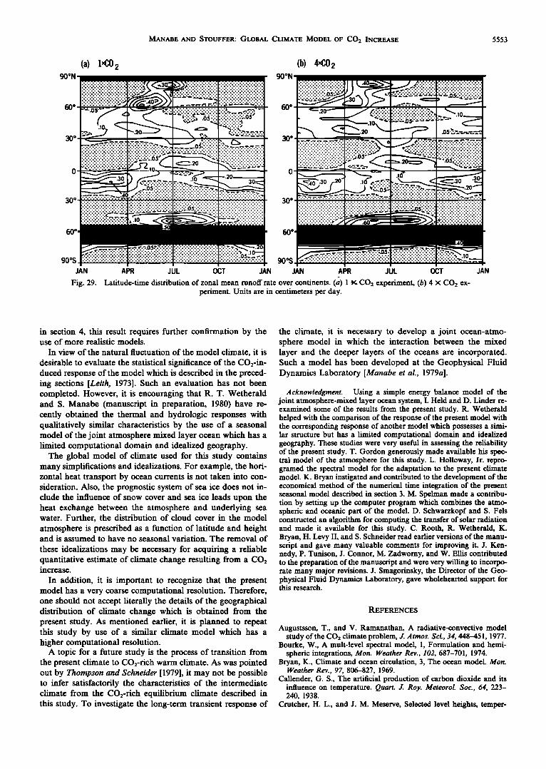
MANABE AND STOUFFER: GLOBAL CLIMATE MODEL OF CO2 INCREASE 5553
60 ø
0
(a) 1,,C0 2 (b) 4,,C02
30'
...........,..........................•, ............................ .'.:..'.:.:.:.:-: :::::::::::::::::::::::::::::
..'-:.:.:.:.:-:-:-.'-:-:..'-:.:.: ;-:-'" • .'C:'.•.:d.•.'.:.:.:.:.: :.:.:.:.:.:.:.:.:.:.:.:.:-:. ':':':':':':':':': .05:'"• :,:,•:.:,:.• -_._. a..• .._..:. 0 "-'-'"-'"'"' .__............................. ..,.,.• .-.
5•• ••• v.v.v.-.v.v.v.......• •"--' .0 < • • -• ,- ;,'<-;.:-;.•'-:,•:.;.;.;..;.;...•..-•.'7...;•;• '• ••.'.'.'.'.'. -;-'.;-;.;.;-;.;.;-;.;..'..•,, • lt• • v....:, 0$.v ..........-...•,.ua •-• • •'•'; '
., .•0 • •• • •%:':':'" .7.•.•• _.._ ,..-.•..•...__. ••..,v.- .... .--, •x, • ,':';':>•. • • ,-:...•..?..-.-..•..?...-: •..F..7...-..T.x•X• • •,• •,:.'..7.--..?..:,..-..-..-v.,7...-...0'.':'.: '..':'.':'.'.'.'.'.'.';'.'.'.'.' ';';';'";'.'-".'-•.•-.--- ,. ..... 05;;;;'-;.;;; ;.."'..•..--•..--.':.-?.r.....Z .;...'...;.;.;.;.;.;.;.;.;.;.; ;.;.;.;.;.;.;.;.;.;.x•,• ...,,•?..;.;.:.;.;.;.;....;..-....;.;.;.;,;.;.;.;.;.;.
i:i:i:i:!:i:i:i:i:!:i:!:i:i:i i:i:!:i:i:i:i:i:i:i:::'•:•' •'*'•':'•'"":::::::: :::::::::::::::::::::::::::::: ============================= :::::::::::::::?Y ================================================
"•*'•:':':'¾'•'•'*a ;-•.•0,"'- -•C "'ff';'•:•""•'-'-'i _ •.30. ) .•,,• ....... 10 •--' •1 •.--•"• 30 /- 10 e, --•"'" .... -•,.•< •.30 '-.-. • • I "%".":-:':':-:-: :-:•-.'•..--.-_'"•---• •,,._.•.•-.•' •.•0; _ ß. •..:.:.:.:.: ..?..-..-. \ V .-.' :, .-.,,'.-.-.-.-.-.-•. __ .20 • ,,•,.-..•:-:.:.:.:.:..:.:.:.:.:.:.:.:.:.:?.-. • _•i •v•_•_•j•,•_ • -.o• ,............................•:•..•..• • •'.'.'.'.'.'.'.'.'.'.'.' ................................?..•.•............• _-7'.'•.'."C.'?.'.•'•'.•.•.'•"•.•.':':-•':-:-:-:-:'•-:-:': :':'X-X-X-X-X-X- '.'.'. ß -- .... '.'.'.'.'-' '.'.'.'-'.'.'-'.'-? ..... •-'-•-?C-•-•.?.•-•-•.7 •'•':-•C-•-•'•'_ _?-_'.'_' -;-:-:-:-:-;-:-;-:¾;¾:-;' ,,-:-;-:¾:-:-:-:-;-:-:-:-:-; :-;-;-:-;-:-:-:-:-:-:-:-:-:- -:-:-:-:-:-;':':-:-:-:-:-:-:' ß ........................................................ ::::::::::::::::::::::::::::: ::::::::::::::::::::::::::::: -:._-:.;:½.05;_;:-:-::::::;.: :.:.;-:.:.:.:.:.:.:-:.:-:.:-; ::::::::::::::::::::::::::::: ::;::;;;::;:;;::::?•;•' ;;•.'•'-";:.;.05•:;:;::: ::::::::::::::::::::::::::::
.:.:.:.:.:.:.;.;.:.;.:.;.::½. ,c.,..•_• "" '•., ,.;.;.:.:.;.:.;.:.;.;.;.;.:.; :.:::.:.:-:.:.x;;;:":"•.-•""--•-•::.;: :::::::::::::::::::::::::::::: ......................,, .•,••...- •i......... .... ..........
,,oo, ::::::::::::::::::::::::::::: :.:.:.:.:.:.:.:.:.:.:.:.:.:..:.:.:.:.:.:.:.:.:.:.:.:.:.:, JAN APR JUL OCT JAN JAN APR JUL OCT JAN
Fig. 29. Latitude-time distribution of zonal mean runoff rate over continents. (•) 1 ,•<, CO: experiment, (b) 4 x CO: ex- periment. Units are in centimeters per day.
in section 4, this result requires further confirmation by the use of more realistic models.
In view of the natural fluctuation of the model climate, it is
desirable to evaluate the statistical significance of the CO:-in- duced response of the model which is described in the preced- ing sections [Leith, 1973]. Such an evaluation has not been completed. However, it is encouraging that R. T. Wetheraid and S. Manabe (manuscript in preparation, 1980) have re- cently obtained the thermal and hydrologic responses with qualitatively similar characteristics by the use of a seasonal model of the joint atmosphere mixed layer ocean which has a limited computational domain and idealized geography.
The global model of climate used for this study contains many simplifications and idealizations. For example, the hori- zontal heat transport by ocean currents is not taken into con- sideration. Also, the prognostic system of sea ice does not in- dude the influence of snow cover and sea ice leads upon the heat exchange between the atmosphere and underlying sea water. Further, the distribution of cloud cover in the model atmosphere is prescribed as a function of latitude and height and is assumed to have no seasonal variation. The removal of
these idealizations may be necessary for acquiring a reliable quantitative estimate of climate change resulting from a CO: increase.
In addition, it is important to recognize that the present model has a very coarse computational resolution. Therefore, one should not accept literally the details of the geographical distribution of climate change which is obtained from the present study. As mentioned earlier, it is planned to repeat this study by use of a similar climate model which has a higher computational resolution.
A topic for a future study is the process of transition from the present climate to CO:-rich warm climate. As was pointed out by Thompson and Schneider [1979], it may not be possible to infer satisfactorily the characteristics of the intermediate climate from the CO:-rich equilibrium climate described in this study. To investigate the long-term transient response of
the climate, it is nebessary to develop a joint ocean-atmo- sphere model in which the interaction between the mixed layer and the deeper layers of the oceans are incorporated. Such a model has been developed at the Geophysical Fluid Dynamics Laboratory [Manabe et al., 1979a].
Acknowledgment. Using a simple energy balance model of the joint atmosphere-mixed layer ocean system, I. Held and D. Linder re- examined some of the results from the present study. R. Wetheraid helped with the comparison of the response of the present model with the corresponding response of another model which possesses a simi- lar structure but has a limited computational domain and idealized geography. These studies were very useful in assessing the reliability of the present study. T. Gordon generously made available his spec- tral model of the atmosphere for this study. L. Holloway, Jr. repro- gramed the spectral model for the adaptation to the present climate model. K. Bryan instigated and contributed to the development of the economical method of the numerical time integration of the present seasonal model described in section 3. M. Spelman made a contribu- tion by setting up the computer program which combines the atmo- spheric and oceanic part of the model. D. Schwarzkopf and S. Fels constructed an algorithm for computing the transfer of solar radiation and made it available for this study. C. Rooth, R. Wetheraid, K. Bryan, H. Levy II, and S. Schneider read earlier versions of the manu- script and gave many valuable comments for improving it. J. Ken- nedy, P. Tunison, J. Connor, M. Zadworny, and W. Ellis contributed to the preparation of the manuscript and were very willing to incorpo- rate many major revisions. J. Smagorinsky, the Director of the Geo- physical Fluid Dynamics Laboratory, gave wholehearted support for this research.
REFERENCES
Augustsson, T., and V. Ramanathan, A radiative-convective model study of the COe climate problem, J. Atmos. ScL, 34, 448-451, 1977.
Bourke, W., A muir-level spectral model, 1, Formulation and hemi- spheric integrations, Mon. Weather Rev., 102, 687-701, 1974.
Bryan, K., Climate and ocean circulation, 3, The ocean model. Mon. Weather Rev., 97, 806-827, 1969.
Callender, G. S., The artificial production of carbon dioxide and its influence on temperature. Quart. J. Roy. Meteorol. Soc., 64, 223- 240, 1938.
Crutcher, H. L., and J. M. Meserve, Selected level heights, temper-
5554 MANABE AND STOUFFER: GLOBAL CLIMATE MODEL OF CO2 INCREASE
ature, and dew points for the Northern Hemisphere, NA FAIR 50- IC-52, U.S. Nav. Weather Ser., Washington, D.C., 1970.
Eliassen, E., B. Machenhauer, and E. Rasmussen, On a numerical method for integration of the hydrodynamical equations with a spectral representation of the horizontal fields, Reœ. 2, Dep. of Me- teorol., Copenhagen Univ., Denmark, 1970.
Ellis, J. S., and T. H. Vonder Haar, Zonal average earth radiation budget measurement from satellite for climate studies, Atmos. $ci. Pap. 240, Colo. State Univ., Fort Collins, Colo., 1976.
Gordon, T., and B. Stem, The GARP programme on numerical ex- perimentation, Reœ. 7, World Meteorol. Org., Geneva, 1974.
Held, I. M., Time Dependent Statistical Dynamical Model of Various Shape and Sizes, World Meteorological Organization, Geneva 1977.
Hering, W. S., and T. R. Borden, Jr., Ozonezonde observation over North America, Environ. Res. Pap. 38(2), Air Force Cambridge Res. Lab., Hanson Field, Mass., 1964.
Holloway, J. L., Jr., and S. Manabe, Simulation of climate by a global general circulation model. Mon. Weather Rev., 101, 69-78, 1971.
Hoskins, B. J., and A. J. Simmons, A multi-layer spectral model and the semi-implicit method, Quart. J. Roy. Meteorol. Soc., 101, 637- 655, 1975.
Kaplan, L. D., The influence of carbon dioxide variations on the at- mospheric heat balance, Tellus, 12, 204-208, 1960.
Koemer, R. M., The mass balance of the sea ice of the Arctic Ocean. J. Glaciol., 12, 173-185, 1973.
Kondratiev, K., and H. I. Niilisk, On the question of carbon dioxide variation in the atmosphere, Geofis. Pura. Appl., 46, 216-230, 1960.
Kung, E. C., R. A. Bryson, and D. H. Lenshow, Study of a continen- tal surface albedo on the basis of flight measurement and structure of the earth's surface cover over North America, Mon. Weather Rev., 92, 543-564, 1964.
Lacis, A. A., and J. E. Hansen, A parameterization for the absorption of solar radiation in the earth's atmosphere, J. Atmos. Sci., 31, 118- 133, 1974.
Leith, C. E., Standard error of time-average estimates of climatic means, J. Appl. Meteorol., 12, 1066-1069, 1973.
Levitus, S., and A. H. Oort, Global analysis of oceanographic data, Bull. Amer. Meteorol. Soc., 58, 1270-1284, 1977.
London, J., A study of the atmospheric heat balance, final report, Contract AF19(122)-165, DDCAD 117227, Coil. of Eng., New York Univ., 1957.
London, J., Mesospheric Dynamics, 3, The distribution of total ozone in the Northern Hemisphere, Final Report, Contract AF19(604)- 5492, Dep. of Meteorol. and Oceanogr., New York Univ., 1962.
Manabe, S., Climate and ocean circulation, 1, The atmospheric circu- lation and the hydrology of the earth's surface, Mon. Weather Rev., 97, 739-774, 1969a.
Manabe, S., Climate and ocean circulation, 2, The atmospheric circu- lation and the effect of heat transport by ocean currents, Mon. Weather Rev., 97, 775-805, 1969b.
Manabe, S., and K. Bryan, Climate calculation with a combined ocean-atmospheric model, J. Atmos. Sci., 26, 786-789, 1969.
Manabe, S., and R. J. Stouffer, A CO2-climate sensitivity study with a mathematical model of the global climate, Nature, 282, 491-493, 1979.
Manabe, S., and R. T. Wetheraid, Thermal equilibrium of the atmo- sphere with a given distribution of relative humidity, J. Atmos. Sci., 24, 241-259, 1967.
Manabe, S., and R. T. Wetherald, The effects of doubling the CO2- concentration on the climate of a general circulation model, J. Atmos. Sci., 32, 3-15, 1975.
Manabe, S., and R. T. Wetheraid, On the distribution of climate change resulting from an increase in CO2-content of the atmo- sphere, J. Atmos. Sci., 37, 99-118, 1980.
Manabe, S., J. Smagorinsky, and R. F. Strickler, Simulated climatol- ogy of a general circulation model with a hydrologic cycle, Mort. Weather Rev., 93, 769-798, 1965.
Manabe, S., K. Bryan, and M. J. Spelman, A global ocean-atmo- sphere climate model with seasonal variation for future studies of climate sensitivity, Dyn. Atmos. Oceans, 3, 393-426, 1979a.
Manabe, S., D. G. Hahn, and J. L. Holloway, Climate simulation with GFDL spectral models of the atmosphere, GARP Publ. Ser. 22, World Meteorol. Org., Geneva, 1979b.
M611er, F., Quarterly charts of rainfall for the whole earth (in Ger- man), Petermanns. Geograph. Mitt., 95, 1-7, 1951.
M611er, F., On the influence of changes in air on the radiation balance of the earth's surface and on the climate, J. Geophys. Res., 68, 3877- 3886, 1963.
National Academy of Sciences, Carbon dioxide and climate: A Scien- tific assessment, Washington, D.C., 1979.
Orsag, S. A., Transform method for calculation of vector-coupled sums: Application to the spectral form of the vorticity equation, J. Atmos. $ci., 27, 890-895, 1970.
Phillips, N. A., A coordinate system having some special advantage for numerical forecasting, J. Meteorol., 14, 184-185, 1957.
Plass, G. N., The influence of 15-micron carbon dioxide band on the atmospheric infrared cooling rate, Quart. J. Roy. Meteorol., Soc., 82, 310-324, 1956.
Platzman, G. W., The spectral form of the vorticity equation, J. Mete- orol., 17, 635-644, 1960.
Posey, J. W., and P. F. Clapp, Global distribution of normal surface albedo, Geof Int., 4, 33-48, 1964.
Ramanathan, V., and J. A. Coakley, Jr., Climate modeling through radiative-convective models, Rev. Geophys. Space Phys., 16, 465- 489, 1978.
Ramanathan, V., R. D. Lian, and R. D. Cess, Increased atmospheric CO2: Zonal and seasonal estimates of the effect on the radiation en- ergy balance and surface temperature, J. Geophys. Res., 84, 4949- 4958, 1979.
Robert, A., The integration of a low order spectral form of the primi- tive equations, J. Meteorol. $oc. Jap., 44, 237-244, 1966.
Rodgers, C. D., and C. D. Walshaw, The computation of infrared cooling rate in planetary atmospheres, Quart. J. Roy. Meteorol. $oc., 92, 67-92, 1966.
Sasamori, T., J. London, and D. V. Hoyt, Radiation budget of South- ern Hemisphere, in Meteorology of the Southern Hemisphere, Mete- orol. Monogr., vol. 13, edited by C. W. Newton, American Meteor- ological Society, Boston, Mass., 1972.
Sellers, W. D., A reassessment of the effect of CO2 variations on a simple global climate model, J. Appl. Meteorol., 13, 831-833, 1974.
Stone, H. M., and S. Manabe, Comparison among various numerical models designed for computing infrared cooling, Mon. Weather Rev., 96, 735-741, 1968.
Taljaad, J. J., H. van Loon, H. L. Crutcher, and R. L. Jenne, Climate of the upper air, 1, Southern Hemisphere, NA FAIR 50-1C-55, U.S. Nav. Weather Ser., Washington, D.C., 1969.
Thompson, S. L., and S. H. Schneider, A seasonal zonal energy bal- ance climate model with an interactive lower layer. J. Geophys. Res., 84, 2401-2414, 1979.
U.S. Naval Oceanographic Office, Oceanographic Atlas of the Polar Seas, 1, Antarctic, Hydrogr. Office Publ. 705, Washington, D.C., 1957.
U.S. Naval Oceanographic Office, Oceanographic Atlas of the Polar Seas, 2, Arctic, Hydrogr. Office Publ. 705, Washington, D.C., 1958.
Wetheraid, R. T., and S. Manabe, The effect of changing solar con- stant on the climate of a general circulation model, J. Atmos. Sci., 32, 2044-2059, 1975.
Wiesnet, D. R., and M. Matson, The satellite-derived Northern Hemi- sphere snow cover record for the winter of 1977-1978, Mon. Weather Rev., 107, 928-933, 1979.
(Received January 23, 1980; revised May 5, 1980;
accepted May 11, 1980.)