Embed Size (px)
Citation preview
MA10CH11-Rohling ARI 20 October 2017 14:47
Annual Review of Marine Science
Comparing Climate Sensitivity,Past and PresentEelco J. Rohling,1,2,∗ Gianluca Marino,1,∗
Gavin L. Foster,2 Philip A. Goodwin,2
Anna S. von der Heydt,3 and Peter Kohler4
1Research School of Earth Sciences, The Australian National University, Canberra 2601,Australia; email: [email protected], [email protected] and Earth Science, University of Southampton, Southampton SO14 3ZH, UnitedKingdom; email: [email protected], [email protected] for Marine and Atmospheric Research Utrecht and Center for Extreme Matter andEmergent Phenomena, Utrecht University, 3584 CC Utrecht, The Netherlands;email: [email protected] Helmholtz-Zentrum fur Polar-und Meeresforschung (AWI), 27515Bremerhaven, Germany; email: [email protected]
Annu. Rev. Mar. Sci. 2018. 10:261–88
First published as a Review in Advance onSeptember 22, 2017
The Annual Review of Marine Science is online atmarine.annualreviews.org
https://doi.org/10.1146/annurev-marine-121916-063242
Copyright c© 2018 by Annual Reviews.All rights reserved
∗These authors contributed equally to this article
Keywords
climate sensitivity, present climate, paleoclimate, idealized scenarios,feedbacks
Abstract
Climate sensitivity represents the global mean temperature change causedby changes in the radiative balance of climate; it is studied for bothpresent/future (actuo) and past (paleo) climate variations, with the formerbased on instrumental records and/or various types of model simulations.Paleo-estimates are often considered informative for assessments ofactuo-climate change caused by anthropogenic greenhouse forcing, butthis utility remains debated because of concerns about the impacts ofuncertainties, assumptions, and incomplete knowledge about controllingmechanisms in the dynamic climate system, with its multiple interactingfeedbacks and their potential dependence on the climate background state.This is exacerbated by the need to assess actuo- and paleoclimate sensitivityover different timescales, with different drivers, and with different (dataand/or model) limitations. Here, we visualize these impacts with idealizedrepresentations that graphically illustrate the nature of time-dependentactuo- and paleoclimate sensitivity estimates, evaluating the strengths,weaknesses, agreements, and differences of the two approaches. We alsohighlight priorities for future research to improve the use of paleo-estimatesin evaluations of current climate change.
261
Click here to view this article's online features:
• Download figures as PPT slides• Navigate linked references• Download citations• Explore related articles• Search keywords
ANNUAL REVIEWS Further
Ann
u. R
ev. M
ar. S
ci. 2
018.
10:2
61-2
88. D
ownl
oade
d fr
om w
ww
.ann
ualr
evie
ws.
org
Acc
ess
prov
ided
by
Aus
tral
ian
Nat
iona
l Uni
vers
ity o
n 06
/03/
19. F
or p
erso
nal u
se o
nly.
MA10CH11-Rohling ARI 20 October 2017 14:47
1. INTRODUCTION
Studies of past and future climate change often center on some climate sensitivity to changes in theradiative balance of the Earth. This sensitivity appears in many guises. The equilibrium climatesensitivity (ECS) is the equilibrium global annual mean temperature rise caused by a doubling ofatmospheric CO2 concentration (Charney et al. 1979, Knutti & Hegerl 2008, IPCC 2013, Forster2016, Stevens et al. 2016) or a radiative forcing of approximately 3.7 W m−2 (Myhre et al. 1998,Byrne & Goldblatt 2014, Etminan et al. 2016), which can be further amplified or dampened byseveral feedbacks within the climate system acting on many different timescales (e.g., von derHeydt et al. 2016). The amount of global annual mean temperature change in response to a givenchange in Earth’s radiative balance is called either the climate sensitivity parameter or the specificclimate sensitivity (in K W−1 m2 or ◦C W−1 m2). The transient climate response is the globalannual mean temperature rise at the time of CO2 doubling, which arises from a linear increase(1% y−1) in CO2 forcing over a period of 70 years (IPCC 2013).
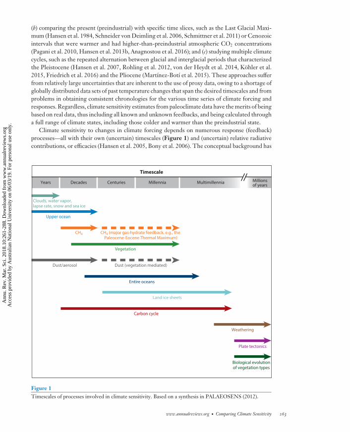
Regardless of which definition or timescale is considered, the response (or sensitivity) of climate(or temperature) to a perturbation in the radiative balance (or forcing) is an important metric forevaluating the potential outcomes of anthropogenic impacts on the radiative balance, such asgreenhouse-gas releases, land-use changes, and aerosol emissions. The radiative balance, in turn,represents the sum of radiative forcings and feedbacks (where the latter occur over a wide range oftimescales) (Figure 1), which collectively determine the surface temperature on Earth. Feedbacksare commonly categorized as fast (when acting within less than 100 years) or slow (when actingover longer timescales), although this timescale-based distinction is somewhat blurry in reality(see overview in PALAEOSENS 2012) (Figure 1).
Attempts at constraining climate sensitivity have been made throughout the past century andearlier, and despite advances in our understanding of the physical processes that govern Earth’sclimate, the estimates have not changed much from the very earliest ones (Arrhenius 1896,Callendar 1938, IPCC 2013, Stevens et al. 2016). Current estimates of climate sensitivity re-main within a 66% probability range of 1.5–4.5 K (Charney et al. 1979, IPCC 2013, Stevens et al.2016). But research into this climate metric has intensified in recent years, notably because ofincreasing concerns about our future global warming trajectory and implementation of mitigationstrategies (Mann 2014). Climate sensitivity has been extensively investigated in studies that linkobservations and modeling both for past (paleo) climates (e.g., Lunt et al. 2010) and for the modernclimate with projections into the future (e.g., Fasullo & Trenberth 2012, Sherwood et al. 2014).Another intensive branch of research estimates climate sensitivity directly from paleoclimate re-constructions (Hansen & Sato 2012, PALAEOSENS 2012, Skinner 2012, Royer 2016, von derHeydt et al. 2016). An emerging property of recent investigations into present-day ECS is someapparent nonlinearity or climate-background-state dependence (Knutti & Rugenstein 2015). Inthe typical approach to calculating ECS—extrapolating transient climate simulations following anabrupt doubling of CO2 (i.e., 2×CO2) to the point when the surface temperature change becomeszero—it turns out that a linear relationship is not the best approximation (Bloch-Johnson et al.2015) and that the so-called fast feedbacks are still changing after more than 150 years (Rugensteinet al. 2016b). These are key issues for further research. In addition, there is interest in better un-derstanding climate sensitivity and the forcing and feedback processes that control Earth’s climatethrough past episodes of climate change, such as the Plio-Pleistocene glacial-interglacial cyclesand earlier Cenozoic events and sustained episodes of global warming. In this field, potential statedependence is also a key focus.
Paleoclimate data can be used to evaluate climate sensitivity in several ways, including(a) analyzing time series of the recent past, such as the last millennium (Hegerl et al. 2006);
262 Rohling et al.
Ann
u. R
ev. M
ar. S
ci. 2
018.
10:2
61-2
88. D
ownl
oade
d fr
om w
ww
.ann
ualr
evie
ws.
org
Acc
ess
prov
ided
by
Aus
tral
ian
Nat
iona
l Uni
vers
ity o
n 06
/03/
19. F
or p
erso
nal u
se o
nly.
MA10CH11-Rohling ARI 20 October 2017 14:47
(b) comparing the present (preindustrial) with specific time slices, such as the Last Glacial Maxi-mum (Hansen et al. 1984, Schneider von Deimling et al. 2006, Schmittner et al. 2011) or Cenozoicintervals that were warmer and had higher-than-preindustrial atmospheric CO2 concentrations(Pagani et al. 2010, Hansen et al. 2013b, Anagnostou et al. 2016); and (c) studying multiple climatecycles, such as the repeated alternation between glacial and interglacial periods that characterizedthe Pleistocene (Hansen et al. 2007, Rohling et al. 2012, von der Heydt et al. 2014, Kohler et al.2015, Friedrich et al. 2016) and the Pliocene (Martınez-Botı et al. 2015). These approaches sufferfrom relatively large uncertainties that are inherent to the use of proxy data, owing to a shortage ofglobally distributed data sets of past temperature changes that span the desired timescales and fromproblems in obtaining consistent chronologies for the various time series of climate forcing andresponses. Regardless, climate sensitivity estimates from paleoclimate data have the merits of beingbased on real data, thus including all known and unknown feedbacks, and being calculated througha full range of climate states, including those colder and warmer than the preindustrial state.
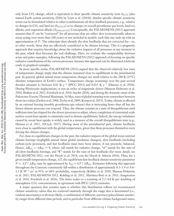
Climate sensitivity to changes in climate forcing depends on numerous response (feedback)processes—all with their own (uncertain) timescales (Figure 1) and (uncertain) relative radiativecontributions, or efficacies (Hansen et al. 2005, Bony et al. 2006). The conceptual background has
Clouds, water vapor, lapse rate, snow and sea ice
Upper ocean
CH4 CH4 (major gas-hydrate feedback, e.g., the Paleocene-Eocene Thermal Maximum)
Vegetation
Dust/aerosol Dust (vegetation mediated)
Entire oceans
Land ice sheets
Carbon cycle
Weathering
Biological evolutionof vegetation types
Plate tectonics
Timescale
Years Decades Centuries Millennia Multimillennia Millionsof years
Figure 1Timescales of processes involved in climate sensitivity. Based on a synthesis in PALAEOSENS (2012).
www.annualreviews.org • Comparing Climate Sensitivity 263
Ann
u. R
ev. M
ar. S
ci. 2
018.
10:2
61-2
88. D
ownl
oade
d fr
om w
ww
.ann
ualr
evie
ws.
org
Acc
ess
prov
ided
by
Aus
tral
ian
Nat
iona
l Uni
vers
ity o
n 06
/03/
19. F
or p
erso
nal u
se o
nly.
MA10CH11-Rohling ARI 20 October 2017 14:47
been previously discussed in relation to both modern/future (actuo) climate change and paleocli-mate change (e.g., Charney et al. 1979; Hansen et al. 1984, 2005, 2007, 2008, 2013b; Skinner 2012;Marvel et al. 2016; von der Heydt et al. 2016). PALAEOSENS (2012) synthesized discussions andmathematically evaluated relationships.
Here, we outline the PALAEOSENS (2012) framework and consider its implications and chal-lenges. We then formulate some simple, purely theoretical, graphical representations to illustrateand evaluate the nature of the probability distributions for climate sensitivity in response to anthro-pogenic forcing and through episodes of climate change in the paleoclimate record. We use theseschematic representations to investigate how climate sensitivities from actuo- and paleo-studiescan best be assessed to make them comparable to one another. Finally, we consider implications ofthe results for the potential of narrowing down the climate sensitivity range and/or its dependenceon climate background states.
2. FRAMEWORK
PALAEOSENS (2012) outlined an approach that uses reconstructions of key climate parametersin the geological past to approximate the equilibrium fast-feedback climate sensitivity term thatapplies to actuo-climate studies (Sa, i.e., the ECS calculated when all fast feedbacks and surface-ocean warming have completed). The main issue that needed to be addressed in aligning climatesensitivity estimates from paleoclimate studies with those from actuo-climate studies concernsthe contrasting timescales involved—natural climate change is much slower than anthropogenicclimate change (Crowley 1990, Zeebe et al. 2016). Natural change therefore includes the action offeedbacks that are too slow to be relevant over the next 100–200 years and/or relate to processesthat are not (yet) included in climate models owing to computational limits (e.g., continental icesheets).
One way to address this issue uses the so-called time-dependent climate sensitivity approach,which accounts for both fast and slow feedbacks and allows evaluation of climate sensitivity con-tinuously over timescales that are relevant to both the imminent future and the distant geologicpast (Zeebe 2013). It builds on the notion that fast and slow feedbacks operate continuously in theclimate system, thereby modulating the evolution of climate and its sensitivity to forcing throughtime. In this time-dependent climate sensitivity approach, the fast-feedback climate sensitivity isset (to 3 K), whereas the evolution of the slow feedbacks (carbon cycle, vegetation, low-latitudeglaciers, and polar ice sheets) is modeled using constraints from the paleoclimate record. Thestrength of this approach for future climate projections lies in the comprehensive estimates ofanthropogenic warming (and its duration) that it delivers. For example, it accounts for the im-pacts of warming on the solubility of CO2 in the ocean, which further enhance global warmingby increasing atmospheric CO2 concentrations (Zeebe 2013). Note that this approach relies ona linearization of the climate response around the background climate and applies only to caseswhere the climate system (after a very long time) reaches a unique and true equilibrium. In reality,the climate system may instead (a) exhibit variability on many different timescales (interannual toorbital), with potentially different characteristics under CO2 forcing, and (b) cross tipping pointsthat imply highly nonlinear climate responses (e.g., Drijfhout et al. 2015).
Another approach, which has been more extensively applied, explicitly resolves radiative forc-ing caused by the slow-feedback processes (e.g., ice-sheet albedo, vegetation albedo, and/orgreenhouse-gas concentrations) and then removes their influences from the calculated climatesensitivity (Hansen et al. 2007, Kohler et al. 2010, Masson-Delmotte et al. 2010, PALAEOSENS2012, Rohling et al. 2012, Martınez-Botı et al. 2015). PALAEOSENS (2012) proposed the pa-rameter Sp for paleoclimate sensitivity in terms of temperature change relative to forcing resulting
264 Rohling et al.
Ann
u. R
ev. M
ar. S
ci. 2
018.
10:2
61-2
88. D
ownl
oade
d fr
om w
ww
.ann
ualr
evie
ws.
org
Acc
ess
prov
ided
by
Aus
tral
ian
Nat
iona
l Uni
vers
ity o
n 06
/03/
19. F
or p
erso
nal u
se o
nly.
MA10CH11-Rohling ARI 20 October 2017 14:47
only from CO2 change, which is equivalent to their specific climate sensitivity term S[CO2] [alsonamed Earth system sensitivity (ESS) by Lunt et al. (2010)]. Similar specific climate sensitivityterms can be formulated relative to other (combinations of) slow-feedback processes, e.g., relativeto changes in CO2 and land ice (S[CO2,LI]) or to changes in overall greenhouse-gas levels, land-icealbedo, and vegetation albedo (S[GHG,LI,VG]). Conceptually, the PALAEOSENS (2012) approachassumes that Sp can be “corrected” for all processes that are either slow (conventionally taken tomean acting over more than 100 years) or not included in models, such that one ends up with anapproximation of Sa. The subscripts then identify the slow feedbacks that are corrected for—or,in other words, those that are effectively considered to be climate forcings. This is a pragmaticapproach that requires knowledge about the radiative impacts of all processes at any moment inthe past, which then becomes the real challenge. Here, we evaluate the comparability betweenactuo and paleo examples, following the PALAEOSENS (2012) approach of focusing on specificradiative contributions of the various processes, because this approach can be illustrated relativelyeasily in graphical examples.
In more specific terms, PALAEOSENS (2012) argued that the observed relatively low ratesof temperature change imply that the climate remained close to equilibrium in the preindustrialpast. In general, global annual mean temperature changes are small relative to the 288 K (15◦C)absolute temperature of Earth’s surface. Temperature change (warming) over the past severaldecades amounts to between 0.01 K y−1 (IPCC 2013) and 0.015 K y−1 (Hansen et al. 2010).During Pleistocene deglaciations, it was an order of magnitude slower (Masson-Delmotte et al.2010, Shakun et al. 2012, Friedrich et al. 2016, Snyder 2016), and during the dramatic onset of thePaleocene-Eocene Thermal Maximum, 56 Mya, rates of global warming were somewhere betweenthose two values (Zachos et al. 2006, Zeebe et al. 2009, Kemp et al. 2015). Today, climate is affectedby an external forcing (notably greenhouse-gas release) that is increasing faster than all but thefastest climate processes can respond. Thus, the climate remains in a state of disequilibrium untilsufficient time has elapsed for the slower processes to adjust, where completion of centennial-scalesurface-ocean heat uptake is commonly used to denote equilibrium. Indeed, the energy imbalancecaused by ocean heat uptake is widely used as a measure of the overall disequilibrium state (e.g.,Hansen et al. 2011, 2013a,b, 2017). During most of the preindustrial past, climate feedbackswere close to equilibrium with the global temperature, given that these processes themselves weredriving the climate changes.
For close-to-equilibrium changes in the past, the radiative impacts of the global mean externalclimate forcings (negligible annual mean global insolation changes), slow feedbacks (includingcarbon-cycle processes), and fast feedbacks must have been almost, if not precisely, balanced.Hence, �R[sf ] + �R[ff ] ≈ 0, where �R stands for radiative change, “sf ” stands for the sum ofall (slow-feedback) forcings, and “ff ” stands for the sum of fast feedbacks (for more detail, seePALAEOSENS 2012, von der Heydt et al. 2014, von der Heydt & Ashwin 2016). Thus, for agiven (small) temperature change, �T, the equilibrium fast-feedback climate sensitivity parameterSa= �T / �R[ff ] may be approximated by S[sf ]=�T / �R[sf ]. Estimates following this approachthroughout the Cenozoic consistently fall within a distribution of approximately 0.3–1.9 or 0.6–1.3 K W−1 m2 at 95% or 68% probability, respectively (Kohler et al. 2010, Masson-Delmotteet al. 2011, PALAEOSENS 2012, Rohling et al. 2012, Martınez-Botı et al. 2015, Anagnostouet al. 2016, Friedrich et al. 2016). The latter scales to a warming of 2.2–4.8 K per doubling ofatmospheric CO2 concentrations, in agreement with IPCC (2013) estimates.
A major question that remains open is whether this distribution reflects (a) reconstructedclimate sensitivity values that are scattered randomly through the range that is determined (i.e.,random uncertainty) or (b) more likely, a combination of different, narrower paleoclimate sensitiv-ity ranges from different time periods, and in particular from different climate background states,
www.annualreviews.org • Comparing Climate Sensitivity 265
Ann
u. R
ev. M
ar. S
ci. 2
018.
10:2
61-2
88. D
ownl
oade
d fr
om w
ww
.ann
ualr
evie
ws.
org
Acc
ess
prov
ided
by
Aus
tral
ian
Nat
iona
l Uni
vers
ity o
n 06
/03/
19. F
or p
erso
nal u
se o
nly.
MA10CH11-Rohling ARI 20 October 2017 14:47
which would therefore represent a systematic source of uncertainty (see also Stevens et al. 2016,von der Heydt et al. 2016). Indeed, model-based process studies and theoretical considerationsdrive an expectation that the value of climate sensitivity should depend on the prevailing climatebackground state, because contributing feedback processes may become more or less effective(i.e., their efficacies may change) under different background climate conditions (for attempts todefine different types of state dependence, see, e.g., Crucifix 2006, von der Heydt et al. 2016).Recent work (von der Heydt et al. 2014, 2016; Kohler et al. 2015) suggests that state depen-dence may be detectable with model-based interpretation of the data, but the matter has not beenconclusively resolved owing to uncertainties involved in the data and the (chronological) compar-isons between records. In detail, the state dependence identified by Kohler et al. (2015) resultedmainly from calculation of the land-ice albedo radiative forcing, �R[LI], based on deconvolutionof the global deep-sea benthic oxygen isotope record with three-dimensional ice-sheet models.Another, relatively minor contribution resulted from the latitudinal dependence of changes inincoming insolation, I. Combined, these drove a nonlinear relationship between �R[LI] and sealevel. Earlier approaches used simpler one-dimensional ice-sheet models (van de Wal et al. 2011),did not similarly account for the latitudinal dependence of I (Kohler et al. 2010, PALAEOSENS2012), or approximated �R[LI] as a linear function of sea level (Hansen et al. 2008, Martınez-Botıet al. 2015) and therefore were primed to miss the state dependence detected by Kohler et al.(2015). More recently, Friedrich et al. (2016) found a similar state-dependent, nonlinear rela-tionship between global temperature and radiative forcing anomalies over the last 784,000 years.Briefly, they determined global annual mean temperature variations using a combination of proxyreconstructions from marine sediment cores and simulation results from an Earth system modelof intermediate complexity. The latter was also used to characterize the planetary albedo throughthe last 784,000 years by simulating the radiative impacts of ice sheets, continental shelf inun-dation/exposure, and vegetation cover. The greenhouse-gas forcing was quantified from ice-corerecords. Finally, Friedrich et al. (2016) detected climate sensitivity and its state dependence fromthe local slope of the temperature versus radiative forcing regression, similar to previous studies(e.g., Kohler et al. 2015).
A key cause of state dependence of climate sensitivity—especially with respect to slowfeedbacks—concerns changes in the efficacy of one or more of these feedbacks under differentclimate states, meaning that the radiative contribution of these processes changes through time.For example, a similar unit area of ice has a stronger radiative impact at lower latitudes than athigher latitudes owing to greater amounts of incoming radiation per unit area as the equator is ap-proached; i.e., the efficacy of the ice albedo feedback may be noticeably stronger for lower-latitudeice than for higher-latitude ice. This notion has implications for paleoclimate sensitivity studiesthat consider both maximum and intermediate glaciation states. In another example, large-scaleclustering of continental mass at low latitudes in the Neoproterozoic supercontinent of Rodinia isthought to have amplified the difference between continental reflection and sea-surface absorptionof incoming solar radiation relative to distributions with more continental mass at higher latitudes,which facilitated major global cooling that eventually led to Snowball Earth (Kirschvink 1992),although this influence remains contested (Poulsen et al. 2002). State dependence of climate sen-sitivity may also result from less obvious changes that—in particular for fast feedbacks—are notnecessarily well approximated in terms of efficacy changes. Among these, variations in cloud cov-erage and types are among the least understood parameters in paleoclimate studies, even thoughthey likely exerted a major control on both albedo and retention of outgoing long-wave radiation(e.g., Bony et al. 2015, Zhou et al. 2016).
So far, it is virtually impossible to develop a comprehensive view of past efficacy changes formost feedbacks, which complicates the reconstruction of state dependence in paleodata-based
266 Rohling et al.
Ann
u. R
ev. M
ar. S
ci. 2
018.
10:2
61-2
88. D
ownl
oade
d fr
om w
ww
.ann
ualr
evie
ws.
org
Acc
ess
prov
ided
by
Aus
tral
ian
Nat
iona
l Uni
vers
ity o
n 06
/03/
19. F
or p
erso
nal u
se o
nly.
MA10CH11-Rohling ARI 20 October 2017 14:47
studies. A pragmatic solution is therefore needed. One approach assumes constant efficacies for allfeedbacks and then assesses whether calculated ECSs appear to have been constant or variable withclimate background state. Any inferred variations subsequently become targets for investigating thepotential variability of feedback efficacies. Alternatively, hybrid approaches are possible, in whichfeedback efficacies through time are assessed with climate models. But this technique introducespotential model bias into the primarily observation-based estimates, meaning that subsequentcomparisons with model-based results become somewhat circular.
In the next section, we use highly idealized examples to graphically illustrate (a) the controls onpaleoclimate sensitivity probability distributions, (b) the limitations resulting from data availabilityissues that affect approximations of Sa using S[sf] in paleodata-based studies, and (c) how statedependence caused by temporal changes in feedback efficacy may factor into the reconstructedprobability distributions.
3. ACTUO-CLIMATE VERSUS PALEOCLIMATE SENSITIVITY
As a first step toward more precise assessments of climate sensitivity, PALAEOSENS (2012)advocated strict adherence to specific definitions to avoid conflating information that appliesover different timescales and different climate background states, as tends to occur in broadlygeneralized approaches (Pagani et al. 2010, Snyder 2016). However, although the PALAEOSENS(2012) framework may ensure like-for-like comparisons, it still involves choices and assumptionsthat may affect the outcome (e.g., Skinner 2012). As a consequence, climate sensitivity is morea moving target than a unique fixed number, depending on the choices and assumptions madeand the timescales and climate background states over which it is considered. In addition, fromthe point of view of dynamical systems theory, climate sensitivity is more likely a probabilitydistribution than a single number (von der Heydt & Ashwin 2016), where the distribution arisesnot from randomness or observational errors but from the actual climate-system dynamics thatexhibit state-dependent behavior through their fast-feedback processes. Thus, pertinent questionsremain about the extent to which a determination of S[sf] may provide insight into the Sa that isrelevant to anthropogenic forcing. We explore this with simple, schematic, idealized graphicexample scenarios.
In contrast to most modeling approaches to climate sensitivity, we consider here atime-dependent climate sensitivity S(t) to reflect both the short-term variations and longer-term background-state dependence of S. We follow the general principles laid out above(PALAEOSENS 2012), where S is determined by the radiative balance of the planet and dif-ferent feedbacks enhance or dampen the initial temperature response:
S = �T�R= −1
λP +∑N
i=1 λfi +
∑Mj=1 λs
j
. 1.
Here, the λ terms refer to the strength of different feedback processes (in terms of a feedback factor,in W m−2 K−1), sorted by the timescale on which they act: λP reflects the change in long-waveradiation in the absence of other feedbacks (the so-called Planck feedback), and the superscripts “f”and “s” denote N fast-feedback and M slow-feedback processes, respectively. Note that Equation1 includes the sum of slow feedbacks (the third term in the denominator), which is the versionapplicable for calculating paleoclimate sensitivity in the PALAEOSENS (2012) framework. Foractuo-climate sensitivity, that sum of slow feedbacks is omitted from the denominator.
Generally, feedback factors are assumed to be constant. However, to reflect the state depen-dence of feedbacks, a time-dependent climate sensitivity, S(t), results from the fact that both λf
and λs can be time dependent. For example, the state dependence of fast-feedback processes as
www.annualreviews.org • Comparing Climate Sensitivity 267
Ann
u. R
ev. M
ar. S
ci. 2
018.
10:2
61-2
88. D
ownl
oade
d fr
om w
ww
.ann
ualr
evie
ws.
org
Acc
ess
prov
ided
by
Aus
tral
ian
Nat
iona
l Uni
vers
ity o
n 06
/03/
19. F
or p
erso
nal u
se o
nly.
MA10CH11-Rohling ARI 20 October 2017 14:47
inferred between glacial and interglacial periods (von der Heydt et al. 2014) may be represented bya (long-timescale) variation of λf(t). The different response times in all feedback factors can be re-flected by a delayed growth of the feedback factors for those processes with slower timescales. Thefirst details in this direction were published by Zeebe (2013), who assumed that the slow-feedbackprocesses, λs, grow from zero to their full strength after a certain time delay.
We adopt a similar approach, with a focus on changes in the time domain. However, ourschematic scenarios build up the argument in terms of simple prescribed functions for the radiativecontributions (�R) from the various processes, rather than in terms of feedback responses. We didthis because we aim to graphically compare actuo- and paleo-scenarios, and for paleo-scenariosthe data more directly resolve �R contributions (Hansen et al. 2007, 2008; Kohler et al. 2010;Masson-Delmotte et al. 2010; Rohling et al. 2012).
Our actuo-scenario (Section 3.1) and paleo-scenario (Section 3.2) represent processes that con-trol changes in the radiative balance of climate by means of simple prescribed sigmoidal responsefunctions, with random, uniformly distributed uncertainty ranges that are evaluated in a MonteCarlo–style approach of 1,000 separate instances. Each response function describes a schematictime-dependent development of a radiative anomaly, in which a phase of exponentially increasinggrowth from zero is followed (in a symmetrical manner through time) by a phase of exponen-tially decreasing growth before settling at the stipulated maximum radiative impact of the processconsidered. The various response functions are then summed up, giving a median record of totalradiative change over time and an uncertainty range based on percentile ranges across all MonteCarlo instances. A rough scaling is worked out for each instance to calibrate the record of totalradiative change to one of total temperature change over time. This temperature record is thenused in a ratio relative to the records for component sums �R[ff] and �R[sf] to estimate the impliedSa and S[sf], respectively.
Although our radiative response functions are simple prescribed functions rather than fullyinteractive feedback processes, we aim to use reasonably realistic amplitude scalings (efficacies)for the contributing radiative (feedback) processes in both the actuo- and paleo-scenarios, basedon published numbers for the modern climate and for Pleistocene glacial-interglacial cycles. Weemphasize that the scenarios may not be viewed as in-depth analyses because they do not com-prehensively represent the interactive physics of the climate system. Including the latter woulddeeply entangle the idealized results shown here and confound relationships between the variousclimate sensitivity definitions and their underlying processes, which would make it more difficultto visualize the potential impacts of issues such as limited data availability, unknown past pro-cesses, and fundamental uncertainties. Our idealized example scenarios guide the discussion byvisualizing such impacts (Sections 4.1 and 4.2). Finally, given that our approach—which draws onproxy-based paleo-reconstructions of radiative forcing anomalies (�R) to calculate temperaturechange (�T ) and climate sensitivity (S)—may be less familiar to climate modelers, we end thediscussion with an illustration of how the importance of the time domain might be addressed in afeedback-focused analysis framework (Section 4.3).
3.1. Illustrative Scenario for Actuo-Climate Sensitivity
For the actuo-climate scenario, we consider that, for any given trigger (e.g., greenhouse-gasemissions), a sequence develops of delayed temperature responses (indicated with δ) and ra-diative feedback responses (indicated with �R), all with their own timescales and amplitudes(Table 1). Key responses to be taken into account are the direct warming effect of the emissions,the associated outgoing long-wave radiation cooling response (Planck response), and other typicalvery fast feedbacks, which include changes in water-vapor content, atmospheric lapse rate, and
268 Rohling et al.
Ann
u. R
ev. M
ar. S
ci. 2
018.
10:2
61-2
88. D
ownl
oade
d fr
om w
ww
.ann
ualr
evie
ws.
org
Acc
ess
prov
ided
by
Aus
tral
ian
Nat
iona
l Uni
vers
ity o
n 06
/03/
19. F
or p
erso
nal u
se o
nly.
MA10CH11-Rohling ARI 20 October 2017 14:47
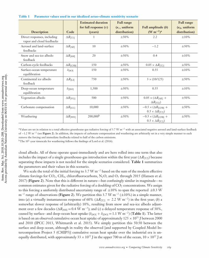
Table 1 Parameter values used in our idealized actuo-climate sensitivity scenario
Description Code
Estimated durationfor full response (τ )
(years)
Full range(ετ , uniformdistribution)
Full amplitude (h)(W m−2)a
Full range(εh, uniformdistribution)
Direct responses, includingvapor and cloud feedbacks
�R[T2] 1 ±50% 2.2 ±10%
Aerosol and land-surfacefeedbacks
�R[AE] 10 ±50% −1.2 ±50%
Snow and sea-ice albedofeedback
�R[SSI] 20 ±50% 0.4 ±10%
Carbon-cycle feedbacks �R[CFB] 150 ±50% 0.05×�R[T2] ±50%
Surface-ocean temperatureequilibration
δ[SO] 150 ±50% 0.55 ±10%
Continental ice albedofeedback
�R[LI] 750 ±50% 3× (10/125) ±50%
Deep-ocean temperatureequilibration
δ[DO] 1,500 ±50% 0.55 ±10%
Vegetation albedo �R[VG] 500 ±50% 0.05× (�R[AE] +�R[T2])
±50%
Carbonate compensation �R[CC] 10,000 ±50% −0.5× (�R[CFB] +0.5×�R[T2])
±50%
Weathering �R[WE] 200,000b ±50% −0.5× (�R[CFB] +0.5×�R[T2])
±50%
aValues are set in relation to a total effective greenhouse-gas radiative forcing of 3.7 W m−2 with an associated negative aerosol and land-surface feedbackof −1.2 W m−2 (see Figure 2). In addition, the impacts of carbonate compensation and weathering are arbitrarily set in a very simple manner to eachremove the forcing and immediate feedbacks related to half of the carbon emissions.bThe 105-year timescale for weathering follows the findings of Lord et al. (2016).
cloud albedo. All of these operate quasi-immediately and are here rolled into one term that alsoincludes the impact of a single greenhouse-gas introduction within the first year (�R[T2]) becauseseparating these impacts is not needed for the simple scenarios considered. Table 1 summarizesthe parameters and their values in this scenario.
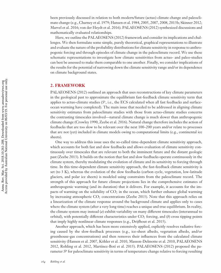
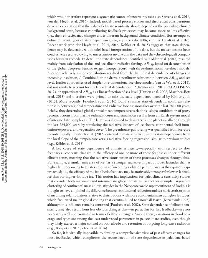
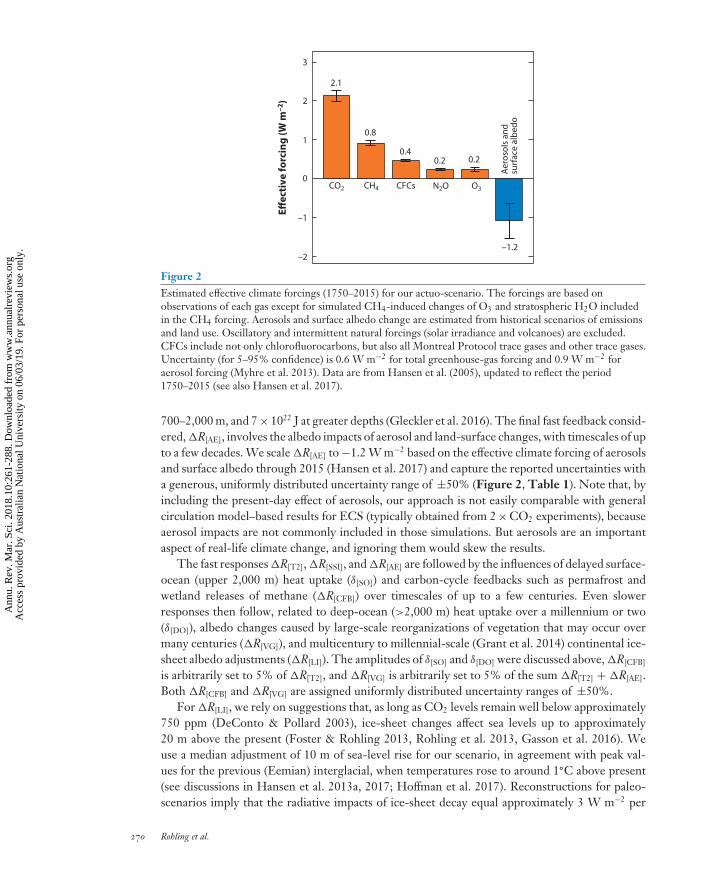
We scale the total of the initial forcing to 3.7 W m−2 based on the sum of the modern effectiveclimate forcings for CO2, CH4, chlorofluorocarbons, N2O, and O3 through 2015 (Hansen et al.2017) (Figure 2). Note that this is different in nature—but confusingly similar in magnitude—tocommon estimates given for the radiative forcing of a doubling of CO2 concentrations. We assignto this forcing a uniformly distributed uncertainty range of ±10% to span the reported ±0.3 Wm−2 range of observations (Figure 2). We partition this 3.7 W m−2 (±10%) in a simple manner,into (a) a virtually instantaneous response of 60% (�R[T2] = 2.2 W m−2) in the first year; (b) asomewhat slower response of (arbitrarily) 10%, resulting from snow and sea-ice albedo adjust-ment over a few decades (�R[SSI]= 0.4 W m−2); and (c) a delayed temperature response of 30%,caused by surface- and deep-ocean heat uptake (δ[SO] + δ[DO]= 1.1 W m−2) (Table 1). The latteris based on an observed cumulative ocean heat uptake of approximately 125× 1021 J between 2000and 2010 (IPCC 2013, Whitmarsh et al. 2015). We simply partition this 50:50 between thesurface and deep ocean, although in reality the observed [and supported by Coupled Model In-tercomparison Project 5 (CMIP5)] cumulative ocean heat uptake over the industrial era is un-equally distributed, with approximately 33× 1022 J in the upper 700 m of the ocean, 10× 1022 J at
www.annualreviews.org • Comparing Climate Sensitivity 269
Ann
u. R
ev. M
ar. S
ci. 2
018.
10:2
61-2
88. D
ownl
oade
d fr
om w
ww
.ann
ualr
evie
ws.
org
Acc
ess
prov
ided
by
Aus
tral
ian
Nat
iona
l Uni
vers
ity o
n 06
/03/
19. F
or p
erso
nal u
se o
nly.
MA10CH11-Rohling ARI 20 October 2017 14:47
2.1
0.8
0.40.2 0.2
–1.2
CO2 CH4 CFCs N2O O3
Aer
osol
s an
dsu
rfac
e al
bedo
2
1
0
–1
Effec
tive
forc
ing
(W m
–2)
3
–2
Figure 2Estimated effective climate forcings (1750–2015) for our actuo-scenario. The forcings are based onobservations of each gas except for simulated CH4-induced changes of O3 and stratospheric H2O includedin the CH4 forcing. Aerosols and surface albedo change are estimated from historical scenarios of emissionsand land use. Oscillatory and intermittent natural forcings (solar irradiance and volcanoes) are excluded.CFCs include not only chlorofluorocarbons, but also all Montreal Protocol trace gases and other trace gases.Uncertainty (for 5–95% confidence) is 0.6 W m−2 for total greenhouse-gas forcing and 0.9 W m−2 foraerosol forcing (Myhre et al. 2013). Data are from Hansen et al. (2005), updated to reflect the period1750–2015 (see also Hansen et al. 2017).
700–2,000 m, and 7× 10²² J at greater depths (Gleckler et al. 2016). The final fast feedback consid-ered, �R[AE], involves the albedo impacts of aerosol and land-surface changes, with timescales of upto a few decades. We scale �R[AE] to−1.2 W m−2 based on the effective climate forcing of aerosolsand surface albedo through 2015 (Hansen et al. 2017) and capture the reported uncertainties witha generous, uniformly distributed uncertainty range of ±50% (Figure 2, Table 1). Note that, byincluding the present-day effect of aerosols, our approach is not easily comparable with generalcirculation model–based results for ECS (typically obtained from 2×CO2 experiments), becauseaerosol impacts are not commonly included in those simulations. But aerosols are an importantaspect of real-life climate change, and ignoring them would skew the results.
The fast responses �R[T2], �R[SSI], and �R[AE] are followed by the influences of delayed surface-ocean (upper 2,000 m) heat uptake (δ[SO]) and carbon-cycle feedbacks such as permafrost andwetland releases of methane (�R[CFB]) over timescales of up to a few centuries. Even slowerresponses then follow, related to deep-ocean (>2,000 m) heat uptake over a millennium or two(δ[DO]), albedo changes caused by large-scale reorganizations of vegetation that may occur overmany centuries (�R[VG]), and multicentury to millennial-scale (Grant et al. 2014) continental ice-sheet albedo adjustments (�R[LI]). The amplitudes of δ[SO] and δ[DO] were discussed above, �R[CFB]
is arbitrarily set to 5% of �R[T2], and �R[VG] is arbitrarily set to 5% of the sum �R[T2] + �R[AE].Both �R[CFB] and �R[VG] are assigned uniformly distributed uncertainty ranges of ±50%.
For �R[LI], we rely on suggestions that, as long as CO2 levels remain well below approximately750 ppm (DeConto & Pollard 2003), ice-sheet changes affect sea levels up to approximately20 m above the present (Foster & Rohling 2013, Rohling et al. 2013, Gasson et al. 2016). Weuse a median adjustment of 10 m of sea-level rise for our scenario, in agreement with peak val-ues for the previous (Eemian) interglacial, when temperatures rose to around 1◦C above present(see discussions in Hansen et al. 2013a, 2017; Hoffman et al. 2017). Reconstructions for paleo-scenarios imply that the radiative impacts of ice-sheet decay equal approximately 3 W m−2 per
270 Rohling et al.
Ann
u. R
ev. M
ar. S
ci. 2
018.
10:2
61-2
88. D
ownl
oade
d fr
om w
ww
.ann
ualr
evie
ws.
org
Acc
ess
prov
ided
by
Aus
tral
ian
Nat
iona
l Uni
vers
ity o
n 06
/03/
19. F
or p
erso
nal u
se o
nly.
MA10CH11-Rohling ARI 20 October 2017 14:47
125-m-equivalent sea-level rise (Hansen et al. 2008, Kohler et al. 2010, Rohling et al. 2012).There remains considerable uncertainty with this number; using three-dimensional ice-sheetmodels, Kohler et al. (2015) found it to be 4 W m−2, whereas Friedrich et al. (2016) reportedit to be only 1.5 W m−2, likely related to a smaller simulated albedo change between land-ice-covered conditions and no-ice conditions relative to that used by Kohler et al. (2015). We use auniformly distributed uncertainty of ±50% of �R[LI], to allow a uniform range between 1.5 and4.5 W m−2 for a 125-m-equivalent sea-level change, which spans the estimates in the literature.Hence, we set the median �R[LI] in the actuo-scenario to 3× (10/125) W m−2 for a sea-levelrise up to 10 m. We accept that use of this linear approximation of �R[LI] from sea-level changeobscures a potentially important nonlinearity of the climate system, which may underpin a statedependence in S[CO2,LI] over the last 2 million years (Kohler et al. 2015).
For each process, the above-mentioned idealized signal-development curve uses the standardfunctional form
�R (t) = (h + εh)
1+ e[−c ( tτ+ετ
−φ)]. 2.
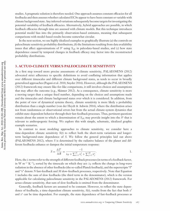
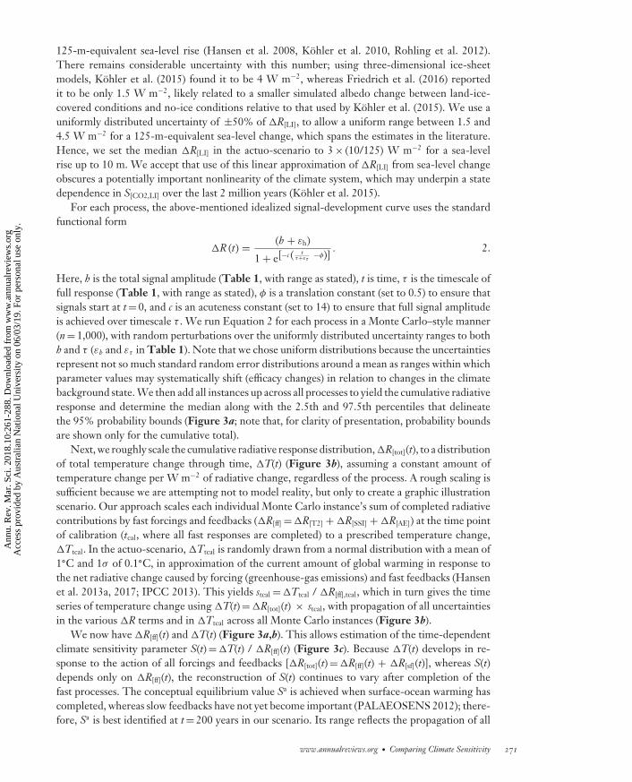
Here, h is the total signal amplitude (Table 1, with range as stated), t is time, τ is the timescale offull response (Table 1, with range as stated), φ is a translation constant (set to 0.5) to ensure thatsignals start at t= 0, and c is an acuteness constant (set to 14) to ensure that full signal amplitudeis achieved over timescale τ . We run Equation 2 for each process in a Monte Carlo–style manner(n= 1,000), with random perturbations over the uniformly distributed uncertainty ranges to bothh and τ (εh and ετ in Table 1). Note that we chose uniform distributions because the uncertaintiesrepresent not so much standard random error distributions around a mean as ranges within whichparameter values may systematically shift (efficacy changes) in relation to changes in the climatebackground state. We then add all instances up across all processes to yield the cumulative radiativeresponse and determine the median along with the 2.5th and 97.5th percentiles that delineatethe 95% probability bounds (Figure 3a; note that, for clarity of presentation, probability boundsare shown only for the cumulative total).
Next, we roughly scale the cumulative radiative response distribution, �R[tot](t), to a distributionof total temperature change through time, �T(t) (Figure 3b), assuming a constant amount oftemperature change per W m−2 of radiative change, regardless of the process. A rough scaling issufficient because we are attempting not to model reality, but only to create a graphic illustrationscenario. Our approach scales each individual Monte Carlo instance’s sum of completed radiativecontributions by fast forcings and feedbacks (�R[ff]=�R[T2] +�R[SSI] +�R[AE]) at the time pointof calibration (tcal, where all fast responses are completed) to a prescribed temperature change,�Ttcal. In the actuo-scenario, �Ttcal is randomly drawn from a normal distribution with a mean of1◦C and 1σ of 0.1◦C, in approximation of the current amount of global warming in response tothe net radiative change caused by forcing (greenhouse-gas emissions) and fast feedbacks (Hansenet al. 2013a, 2017; IPCC 2013). This yields stcal=�Ttcal / �R[ff],tcal, which in turn gives the timeseries of temperature change using �T(t)=�R[tot](t) × stcal, with propagation of all uncertaintiesin the various �R terms and in �Ttcal across all Monte Carlo instances (Figure 3b).
We now have �R[ff](t) and �T(t) (Figure 3a,b). This allows estimation of the time-dependentclimate sensitivity parameter S(t)=�T(t) / �R[ff](t) (Figure 3c). Because �T(t) develops in re-sponse to the action of all forcings and feedbacks [�R[tot](t)=�R[ff](t) + �R[sf](t)], whereas S(t)depends only on �R[ff](t), the reconstruction of S(t) continues to vary after completion of thefast processes. The conceptual equilibrium value Sa is achieved when surface-ocean warming hascompleted, whereas slow feedbacks have not yet become important (PALAEOSENS 2012); there-fore, Sa is best identified at t= 200 years in our scenario. Its range reflects the propagation of all
www.annualreviews.org • Comparing Climate Sensitivity 271
Ann
u. R
ev. M
ar. S
ci. 2
018.
10:2
61-2
88. D
ownl
oade
d fr
om w
ww
.ann
ualr
evie
ws.
org
Acc
ess
prov
ided
by
Aus
tral
ian
Nat
iona
l Uni
vers
ity o
n 06
/03/
19. F
or p
erso
nal u
se o
nly.
MA10CH11-Rohling ARI 20 October 2017 14:47
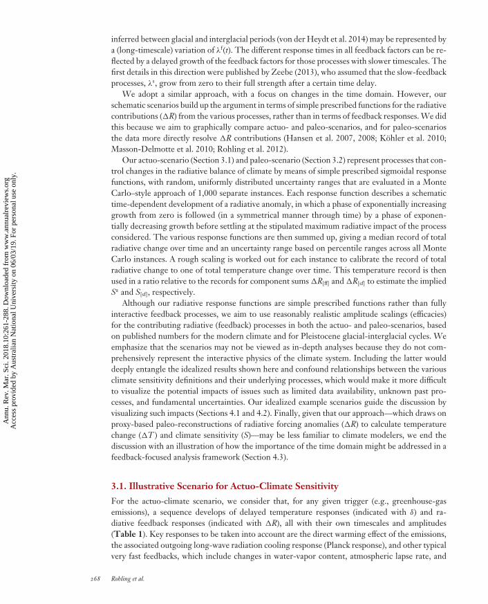
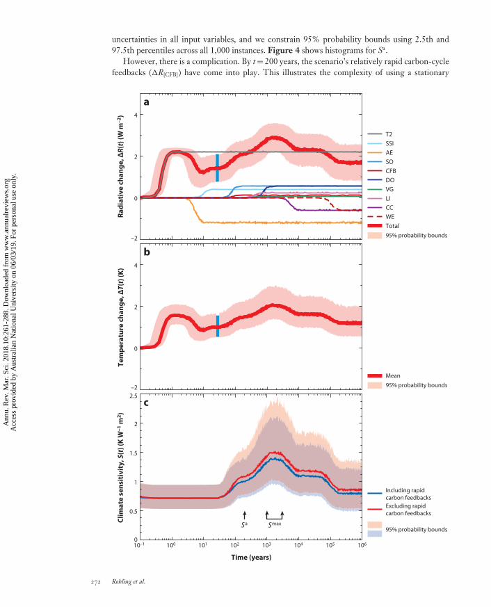
uncertainties in all input variables, and we constrain 95% probability bounds using 2.5th and97.5th percentiles across all 1,000 instances. Figure 4 shows histograms for Sa.
However, there is a complication. By t= 200 years, the scenario’s relatively rapid carbon-cyclefeedbacks (�R[CFB]) have come into play. This illustrates the complexity of using a stationary
–2
0
2
4
Tem
pera
ture
cha
nge,
ΔT(t)
(K)
Mean
10–1 100 101 102 103 104 105 1060
0.5
1
1.5
2
2.5
Clim
ate
sens
itiv
ity,
S(t
) (K
W–1
m2 )
Including rapidcarbon feedbacksExcluding rapidcarbon feedbacks
95% probability bounds
c
b
SmaxSa
Time (years)
–2
0
2
4Ra
diat
ive
chan
ge, Δ
R(t)
(W m
–2)
T2SSIAESOCFBDOVGLICCWETotal
a
95% probability bounds
95% probability bounds
272 Rohling et al.
Ann
u. R
ev. M
ar. S
ci. 2
018.
10:2
61-2
88. D
ownl
oade
d fr
om w
ww
.ann
ualr
evie
ws.
org
Acc
ess
prov
ided
by
Aus
tral
ian
Nat
iona
l Uni
vers
ity o
n 06
/03/
19. F
or p
erso
nal u
se o
nly.
MA10CH11-Rohling ARI 20 October 2017 14:47
Climate sensitivity (K W–1 m2)
50
40
30
20
10
00 0.5 1.0 1.5 2.0 2.5
n
Transient (fast feedbacks only)
Sa without rapid carbon feedbacksSa with rapid carbon feedbacksSmax without rapid carbon feedbacksSmax with rapid carbon feedbacks
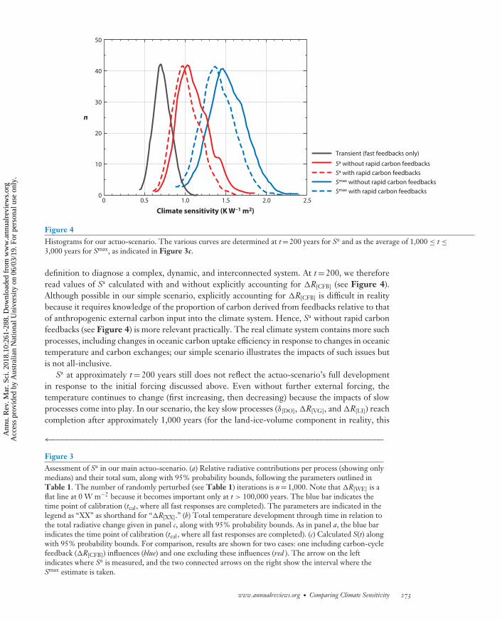
Figure 4Histograms for our actuo-scenario. The various curves are determined at t= 200 years for Sa and as the average of 1,000 ≤ t ≤3,000 years for Smax, as indicated in Figure 3c.
definition to diagnose a complex, dynamic, and interconnected system. At t= 200, we thereforeread values of Sa calculated with and without explicitly accounting for �R[CFB] (see Figure 4).Although possible in our simple scenario, explicitly accounting for �R[CFB] is difficult in realitybecause it requires knowledge of the proportion of carbon derived from feedbacks relative to thatof anthropogenic external carbon input into the climate system. Hence, Sa without rapid carbonfeedbacks (see Figure 4) is more relevant practically. The real climate system contains more suchprocesses, including changes in oceanic carbon uptake efficiency in response to changes in oceanictemperature and carbon exchanges; our simple scenario illustrates the impacts of such issues butis not all-inclusive.
Sa at approximately t= 200 years still does not reflect the actuo-scenario’s full developmentin response to the initial forcing discussed above. Even without further external forcing, thetemperature continues to change (first increasing, then decreasing) because the impacts of slowprocesses come into play. In our scenario, the key slow processes (δ[DO], �R[VG], and �R[LI]) reachcompletion after approximately 1,000 years (for the land-ice-volume component in reality, this
←−−−−−−−−−−−−−−−−−−−−−−−−−−−−−−−−−−−−−−−−−−−−−−−−−−−−−−−−−−−−−−−−−−−−−−Figure 3Assessment of Sa in our main actuo-scenario. (a) Relative radiative contributions per process (showing onlymedians) and their total sum, along with 95% probability bounds, following the parameters outlined inTable 1. The number of randomly perturbed (see Table 1) iterations is n= 1,000. Note that �R[WE] is aflat line at 0 W m−2 because it becomes important only at t > 100,000 years. The blue bar indicates thetime point of calibration (tcal, where all fast responses are completed). The parameters are indicated in thelegend as “XX” as shorthand for “�R[XX].” (b) Total temperature development through time in relation tothe total radiative change given in panel c, along with 95% probability bounds. As in panel a, the blue barindicates the time point of calibration (tcal, where all fast responses are completed). (c) Calculated S(t) alongwith 95% probability bounds. For comparison, results are shown for two cases: one including carbon-cyclefeedback (�R[CFB]) influences (blue) and one excluding these influences (red ). The arrow on the leftindicates where Sa is measured, and the two connected arrows on the right show the interval where theSmax estimate is taken.
www.annualreviews.org • Comparing Climate Sensitivity 273
Ann
u. R
ev. M
ar. S
ci. 2
018.
10:2
61-2
88. D
ownl
oade
d fr
om w
ww
.ann
ualr
evie
ws.
org
Acc
ess
prov
ided
by
Aus
tral
ian
Nat
iona
l Uni
vers
ity o
n 06
/03/
19. F
or p
erso
nal u
se o
nly.
MA10CH11-Rohling ARI 20 October 2017 14:47
may be too fast, given that adjustment over∼3,000 years has been suggested by modeling studies;Clark et al. 2016). From approximately t= 3,000 years, carbonate compensation becomes a playeras the first of the very slow Earth system responses (eventually also including silicate weathering)that slowly remove the carbon. We portray the peak value of S(t) (here named Smax) using thedistribution between t= 1,000 and t= 3,000 years (see Figure 4). If the �R[LI] adjustment timewere stretched to ∼3,000 years (see Clark et al. 2016), Smax would be a narrower peak of similaramplitude, centered on t= 3,000 years.
3.2. Illustrative Scenario for Paleoclimate Sensitivity
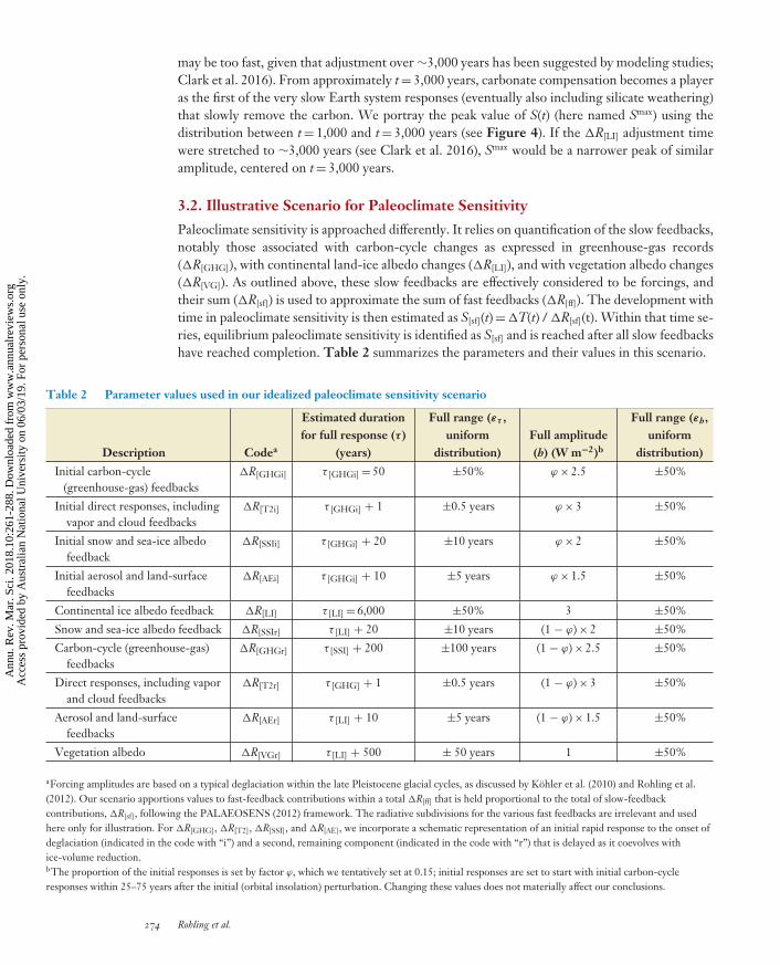
Paleoclimate sensitivity is approached differently. It relies on quantification of the slow feedbacks,notably those associated with carbon-cycle changes as expressed in greenhouse-gas records(�R[GHG]), with continental land-ice albedo changes (�R[LI]), and with vegetation albedo changes(�R[VG]). As outlined above, these slow feedbacks are effectively considered to be forcings, andtheir sum (�R[sf]) is used to approximate the sum of fast feedbacks (�R[ff]). The development withtime in paleoclimate sensitivity is then estimated as S[sf](t)=�T(t) / �R[sf](t). Within that time se-ries, equilibrium paleoclimate sensitivity is identified as S[sf] and is reached after all slow feedbackshave reached completion. Table 2 summarizes the parameters and their values in this scenario.
Table 2 Parameter values used in our idealized paleoclimate sensitivity scenario
Description Codea
Estimated durationfor full response (τ )
(years)
Full range (ετ ,uniform
distribution)Full amplitude(h) (W m−2)b
Full range (εh,uniform
distribution)
Initial carbon-cycle(greenhouse-gas) feedbacks
�R[GHGi] τ [GHGi]= 50 ±50% ϕ× 2.5 ±50%
Initial direct responses, includingvapor and cloud feedbacks
�R[T2i] τ [GHGi] + 1 ±0.5 years ϕ× 3 ±50%
Initial snow and sea-ice albedofeedback
�R[SSIi] τ [GHGi] + 20 ±10 years ϕ× 2 ±50%
Initial aerosol and land-surfacefeedbacks
�R[AEi] τ [GHGi] + 10 ±5 years ϕ× 1.5 ±50%
Continental ice albedo feedback �R[LI] τ [LI]= 6,000 ±50% 3 ±50%
Snow and sea-ice albedo feedback �R[SSIr] τ [LI] + 20 ±10 years (1 − ϕ)× 2 ±50%
Carbon-cycle (greenhouse-gas)feedbacks
�R[GHGr] τ [SSI] + 200 ±100 years (1 − ϕ)× 2.5 ±50%
Direct responses, including vaporand cloud feedbacks
�R[T2r] τ [GHG] + 1 ±0.5 years (1 − ϕ)× 3 ±50%
Aerosol and land-surfacefeedbacks
�R[AEr] τ [LI] + 10 ±5 years (1 − ϕ)× 1.5 ±50%
Vegetation albedo �R[VGr] τ [LI] + 500 ± 50 years 1 ±50%
aForcing amplitudes are based on a typical deglaciation within the late Pleistocene glacial cycles, as discussed by Kohler et al. (2010) and Rohling et al.(2012). Our scenario apportions values to fast-feedback contributions within a total �R[ff] that is held proportional to the total of slow-feedbackcontributions, �R[sf], following the PALAEOSENS (2012) framework. The radiative subdivisions for the various fast feedbacks are irrelevant and usedhere only for illustration. For �R[GHG], �R[T2], �R[SSI], and �R[AE], we incorporate a schematic representation of an initial rapid response to the onset ofdeglaciation (indicated in the code with “i”) and a second, remaining component (indicated in the code with “r”) that is delayed as it coevolves withice-volume reduction.bThe proportion of the initial responses is set by factor ϕ, which we tentatively set at 0.15; initial responses are set to start with initial carbon-cycleresponses within 25–75 years after the initial (orbital insolation) perturbation. Changing these values does not materially affect our conclusions.
274 Rohling et al.
Ann
u. R
ev. M
ar. S
ci. 2
018.
10:2
61-2
88. D
ownl
oade
d fr
om w
ww
.ann
ualr
evie
ws.
org
Acc
ess
prov
ided
by
Aus
tral
ian
Nat
iona
l Uni
vers
ity o
n 06
/03/
19. F
or p
erso
nal u
se o
nly.
MA10CH11-Rohling ARI 20 October 2017 14:47
Conceptually, no immediate agreement might be expected between actuo- and paleoclimatesensitivity estimates because they are determined from processes operating over very differenttimescales, with different assumptions and uncertainties. For example, past climate variationswere not adjustments to very rapid, high-amplitude perturbations (such as the anthropogenic CO2
emissions) along the lines of actuo-climate adjustments, but were triggered by slowly developingprocesses such as orbital forcing, with timescales of many thousands of years. Hence, paleoclimaterecords reflect coevolving changes in all climate-regulating processes (save for the very slowestones, such as plate tectonics) that are either in or near equilibrium with the changing forcing. As aconsequence, most studies based on time series of temperature and slow-feedback change directlyfind the equilibrium value S[sf], although this may not be true in highly resolved studies overcentennial-to-millennial-scale climate fluctuations (see below). In addition, paleoclimate recordsrepresent an integration of all feedback processes; e.g., they include not only the temperatureresponse to CO2 changes, but also the CO2 response to temperature changes. Our simple paleo-scenario allows such complications to be teased apart, to gauge over what timescales signals needto be considered to approximate the desired equilibrium sensitivity and what the consequenceswould be of pushing reconstructions from paleodata into shorter timescales.
For the scale and duration of the processes in our paleo-scenario, we draw on studies of glacialcycles of the last 800,000 years. As such, this scenario may be seen as a rough approximation of adeglaciation. Deglaciations were triggered by orbital forcing of climate, in particular by changesin Northern Hemisphere summer insolation (Hays et al. 1976). Orbital forcing involves minorannual-mean global-mean forcing (�0.5 W m−2) but sets up considerable gradients on spatial(latitudinal) and seasonal scales. For a long time, it was not well understood how these triggereddeglaciations (Shackleton 2000, Denton et al. 2010, Abe-Ouchi et al. 2013), although the timingrelationship was reasonably clear (Hays et al. 1976, Cheng et al. 2016). Recently, a simple modelhas related every deglaciation of the last million years to the crossing of summer insolation througha simple threshold (Tzedakis et al. 2017).
Our paleo-scenario considers an idealized sequence of events inspired by data for the penulti-mate glacial termination (Marino et al. 2015, Holloway et al. 2016) because this termination avoidsthe greater complexity of the last deglaciation yet still has the requisite chronological control forthe relevant climate records (Billups 2015, Marino et al. 2015). Following the initial perturbation(orbital forcing) and fast responses, continental ice-volume changes over thousands of years drovethe further feedback responses mainly through bipolar temperature seesaw processes (Stocker1998, Stocker & Johnsen 2003) that led to rapid Southern Ocean warming and sea-ice reduction,CO2 outgassing, warming and vapor feedbacks, and so on. Here we include aerosol changes inthat suite as well, despite a lack (so far) of unequivocal empirical evidence of that particular cou-pling. There is no unambiguous empirical evidence about the phase relationship of global meanvegetation responses to ice-volume changes, either. But given that we seek only to formulate anillustrative, idealized scenario, we simply assume that key vegetation changes take place withincenturies following land-ice changes.
The orbital-forcing component is ignored here because of our focus on annual-mean global-mean forcing. But it is important in that it directly triggers responses in ice sheets and otherprocesses in the climate system (Schmidt et al. 2017), which cause additional feedback responsesonce the climate begins to change; some of these links develop rapidly, and others develop slowly.For example, small, regionally or seasonally focused warming resulting from orbital forcing trig-gers sea-ice retreat as well as changes in surface albedo and air-sea carbon exchange, which drivefurther warming, and so on. Thereafter, the slow feedbacks come into action, such as land-iceand vegetation albedo changes. When that happens, fast processes keep interacting with slowfeedbacks. Paleo-reconstructions cannot distinguish fast responses associated with slow processes
www.annualreviews.org • Comparing Climate Sensitivity 275
Ann
u. R
ev. M
ar. S
ci. 2
018.
10:2
61-2
88. D
ownl
oade
d fr
om w
ww
.ann
ualr
evie
ws.
org
Acc
ess
prov
ided
by
Aus
tral
ian
Nat
iona
l Uni
vers
ity o
n 06
/03/
19. F
or p
erso
nal u
se o
nly.
MA10CH11-Rohling ARI 20 October 2017 14:47
from the slow processes themselves, or indeed the acceleration of slow processes resulting fromassociated, superimposed fast responses. Note that similar interactions occur in actuo-climatechanges, but our simple actuo-scenario avoids this issue by pragmatically viewing the stipulatedslow-feedback influences as effective net impacts. Doing so in the paleo-scenario would divorceour scenario too much from the paleo-reconstructions, in which temperature (and fast feedbacks)closely coevolve over thousands of years with the slow feedbacks (e.g., Rohling et al. 2009; Grantet al. 2012, 2014). Because our simple paleo-scenario cannot resolve such interactions (a dynamicmodel would be needed), we instead include a crude representation by evaluating the contribu-tion of fast feedbacks to paleoclimate change as a two-stage development. One stage stands forthe initial responses (indicated in Table 2 with “i” in the parameter names), and the other isthe subsequent fast-feedback response (indicated with “r”) associated with the development of thedominant slow continental land-ice feedback (�R[LI]). We tentatively set 0.15:0.85 proportion-alities for this. The proportionality is crudely inspired by early (initial) CO2 jumps that predatesignificant ice-volume/sea-ice responses, at around 16,300, 14,800, and 11,700 years ago, withCO2 levels in each case jumping abruptly by approximately 15% of the total deglacial change(Lambeck et al. 2014, Marcott et al. 2014).
To obtain S[sf], slow feedbacks are effectively considered to be climate forcings in thePALAEOSENS (2012) framework. Our scenario considers the total greenhouse-gas forcingcomponent �R[GHG]. In paleodata studies, this component can be determined from records ofgreenhouse-gas changes (notably from ice cores). These records integrate all carbon-cycle feed-backs, including carbonate compensation and weathering, which therefore need not be consideredseparately. We then add the continental land-ice albedo effect, which can be found from sea-levelreconstructions, giving �R[GHG] + �R[LI]. Finally, the slow vegetation albedo feedback (�R[VG])should be similarly accounted for, but this is substantially challenged by an absence of good globaldata coverage, which definitely needs to be addressed through future research. To date, hardlyany paleo-studies have accounted for �R[VG] (Friedrich et al. 2016 is an exception), and we assessthe implications by showing results that either include or exclude �R[VG]. Our analysis does notinclude albedo changes caused by atmospheric dust (aerosol) variations among the slow feedbacks/forcings, because there is no agreed way to deal with aerosols in paleoclimate sensitivity studiesand because time series of atmospheric dust are geographically very limited and generally qual-itative anyway, so that the aerosol component remains highly speculative and uncertain (e.g.,PALAEOSENS 2012, Rohling et al. 2012).
We roughly calibrate or scale our paleo-scenario on the basis of values for the radiative forc-ings and feedbacks compiled by Kohler et al. (2010) and Rohling et al. (2012) (Table 2), witha total median value of 3 W m−2 for �R[LI] (for discussion, see Section 3.1) and 2.5 W m−2
for �R[GHG]. We use �R[VG]= 1 W m−2, in agreement with Friedrich et al. (2016). As in thePALAEOSENS (2012) framework, we assume that �R[ff] is proportional to �R[sf] over timescalesof more than a few thousand years. On shorter timescales, this assumption cannot be correct be-cause fast feedbacks dominate at first, whereas slow feedbacks become important at a later stage(our results illustrate this). Proportional contributions of individual fast responses are irrelevanthere because our assessment always considers their summed value, but just for illustration’s sake,we have made an attempt at reasonably apportioning them (Table 2). The total median range of�R[AE] is estimated at around 1.5 W m−2, and for snow and sea-ice albedo we use �R[SSI]= 2W m−2, based on discussions by Kohler et al. (2010) and Rohling et al. (2012). This leaves3 W m−2 for the outgoing long-wave radiation response, water-vapor content, atmospheric lapserate, cloud albedo, and so on, all of which are captured in one term, �R[T2]. All radiative termsare assigned ±50% uncertainties using uniform distributions. The paleo-scenario omits δ[SO] andδ[DO] because paleodata yield only the total temperature response, which includes these factors.
276 Rohling et al.
Ann
u. R
ev. M
ar. S
ci. 2
018.
10:2
61-2
88. D
ownl
oade
d fr
om w
ww
.ann
ualr
evie
ws.
org
Acc
ess
prov
ided
by
Aus
tral
ian
Nat
iona
l Uni
vers
ity o
n 06
/03/
19. F
or p
erso
nal u
se o
nly.
MA10CH11-Rohling ARI 20 October 2017 14:47
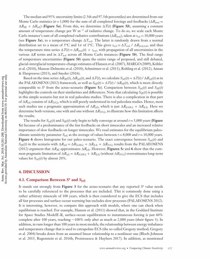
The median and 95% uncertainty limits (2.5th and 97.5th percentiles) are determined from ourMonte Carlo statistics (n= 1,000) for the sum of all completed forcings and feedbacks (�R[tot]=�R[ff] + �R[sf]) (Figure 5a). From this, we determine �T(t) (Figure 5b), assuming a constantamount of temperature change per W m−2 of radiative change. To do so, we scale each MonteCarlo instance’s sum of all completed radiative contributions (�R[tot]), taken at tcal= 10,000 years(see Figure 5a), to a temperature change �Ttcal. The latter is randomly drawn from a normaldistribution set to a mean of 5◦C and 1σ of 1◦C. This gives stcal=�Ttcal / �R[tot],tcal, and thusthe temperature time series �T(t)=�R[tot](t) × stcal, with propagation of all uncertainties in thevarious �R terms and in �Ttcal across all Monte Carlo instances (Figure 5b). The final rangeof temperature uncertainties (Figure 5b) spans the entire range of proposed, and still debated,glacial-interglacial temperature-change estimates of Hansen et al. (2007), MARGO (2009), Kohleret al. (2010), Masson-Delmotte et al. (2010), Schmittner et al. (2011), Rohling et al. (2012), Annan& Hargreaves (2013), and Snyder (2016).
Based on the time series �R[ff](t), �R[sf](t), and �T(t), we calculate S[sf](t)=�T(t) / �R[sf](t) as inthe PALAEOSENS (2012) framework, as well as S[ff](t)=�T(t) / �R[ff](t), which is more directlycomparable to Sa from the actuo-scenario (Figure 5c). Comparison between S[sf](t) and S[ff](t)highlights the controls on their similarities and differences. Note that calculating S[ff](t) is possiblein this simple scenario but not in real paleodata studies. There is also a complication in that partof �R[sf] consists of �R[VG], which is still poorly understood in real paleodata studies. Hence, mostsuch studies use a pragmatic approximation of �R[sf], which is just �R[GHG] + �R[LI]. Here wedetermine both versions, one with and one without �R[VG], to illustrate how this limitation affectsthe results.
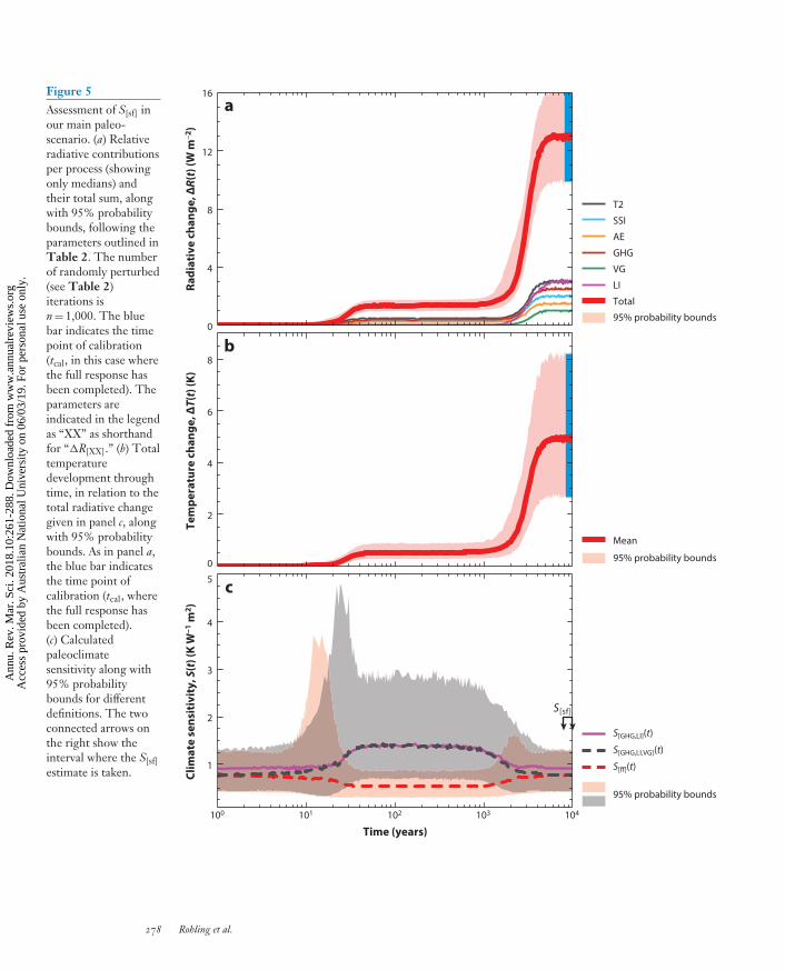
The results for S[sf](t) and S[ff](t) only begin to fully converge at around t= 5,000 years (Figure5c) because of a predominance of the fast feedbacks on short timescales and an increased relativeimportance of slow feedbacks on longer timescales. We read estimates for the equilibrium paleo-climate sensitivity parameter S[sf] as the average of values between t= 8,000 and t= 10,000 years.Figure 6 shows histograms for our paleo-scenario. The exact convergence between S[sf](t) andS[ff](t) in the scenario with �R[sf]=�R[GHG] + �R[LI] + �R[VG] results from the PALAEOSENS(2012) argument that �R[ff] approximates �R[sf]. However, Figures 5c and 6 show that the com-mon pragmatic limitation of �R[sf]=�R[GHG] +�R[LI] (without �R[VG]) overestimates long-termvalues for S[sf](t) by almost 20%.
4. DISCUSSION
4.1. Comparison Between Sa and S[sf]
It stands out strongly from Figure 3 for the actuo-scenario that any reported Sa value needsto be carefully referenced to the processes that are included. This is commonly done using arather arbitrary timescale of 100 years, which is then considered to give the ECS that includesall fast processes and surface-ocean warming but excludes slow processes (PALAEOSENS 2012).It is interesting, however, to compare this approach with models, where one can check whenequilibrium is reached. For example, Hansen et al. (2011) showed that, in the Goddard Institutefor Space Studies ModelE-R, surface-ocean equilibration to instantaneous forcing is just 60%complete after 100 years, reaching ∼100% only after as much as 2,000 years (their figure 3). Inaddition, in runs longer than 100 years in most models, the relationship between energy imbalanceand temperature change that is used to extrapolate ECS (the so-called Gregory method; Gregoryet al. 2004) breaks down from an assumed linear relationship to a nonlinear one (Bloch-Johnsonet al. 2015, Rugenstein et al. 2016b, Proistosescu & Huybers 2017). In addition, as mentioned
www.annualreviews.org • Comparing Climate Sensitivity 277
Ann
u. R
ev. M
ar. S
ci. 2
018.
10:2
61-2
88. D
ownl
oade
d fr
om w
ww
.ann
ualr
evie
ws.
org
Acc
ess
prov
ided
by
Aus
tral
ian
Nat
iona
l Uni
vers
ity o
n 06
/03/
19. F
or p
erso
nal u
se o
nly.
MA10CH11-Rohling ARI 20 October 2017 14:47
0
2
4
6
8
Mean
1
2
3
4
5
S[GHG,LI](t)
S[GHG,LI,VG](t)
S[ff](t)
c
b
100 101 102 103 104
0
4
8
12
16
T2
SSI
AE
GHG
VG
LI
Total
a
S[sf]
Tem
pera
ture
cha
nge,
ΔT(t)
(K)
Time (years)
Radi
ativ
e ch
ange
, ΔR(t)
(W m
–2)
95% probability bounds
95% probability bounds
95% probability bounds
Clim
ate
sens
itiv
ity,
S(t
) (K
W–1
m2 )
Figure 5Assessment of S[sf] inour main paleo-scenario. (a) Relativeradiative contributionsper process (showingonly medians) andtheir total sum, alongwith 95% probabilitybounds, following theparameters outlined inTable 2. The numberof randomly perturbed(see Table 2)iterations isn= 1,000. The bluebar indicates the timepoint of calibration(tcal, in this case wherethe full response hasbeen completed). Theparameters areindicated in the legendas “XX” as shorthandfor “�R[XX].” (b) Totaltemperaturedevelopment throughtime, in relation to thetotal radiative changegiven in panel c, alongwith 95% probabilitybounds. As in panel a,the blue bar indicatesthe time point ofcalibration (tcal, wherethe full response hasbeen completed).(c) Calculatedpaleoclimatesensitivity along with95% probabilitybounds for differentdefinitions. The twoconnected arrows onthe right show theinterval where the S[sf]estimate is taken.
278 Rohling et al.
Ann
u. R
ev. M
ar. S
ci. 2
018.
10:2
61-2
88. D
ownl
oade
d fr
om w
ww
.ann
ualr
evie
ws.
org
Acc
ess
prov
ided
by
Aus
tral
ian
Nat
iona
l Uni
vers
ity o
n 06
/03/
19. F
or p
erso
nal u
se o
nly.
MA10CH11-Rohling ARI 20 October 2017 14:47
n
50
40
30
20
10
00 0.5 1.0 1.5 2.0 2.5
Climate sensitivity (K W–1 m2)
S[ff]
S[GHG,LI,VG]
S[GHG,LI]
PALAEOSENS
Figure 6Histograms for our paleo-scenario. The various curves are determined as the averages of 8,000 ≤ t ≤10,000 years, as indicated in Figure 5c. The gray shading represents a scaled version of the distribution fromPALAEOSENS (2012, their figure 3c).
above, any comparison of our number for Sa with general circulation model–based ECS estimates iscomplicated by the fact that model simulations typically start with a perturbation of CO2 but omitthe observed negative radiative impacts from anthropogenic aerosols and land-surface changes(Figure 2), which act to reduce the temperature rise.
Clearly, even our simple scenario does not neatly separate processes in time. Uncertainties inthe timescales of the various processes and the potential operation of �R[CFB] on similar timescalesto δ[SO] make climate sensitivity a moving target through time (Figure 3). For the example setup here, t= 200 years seems more suitable for determining Sa because all included responses(fast feedbacks) have completed (although this is not fully the case in the more realistic model ofHansen et al. 2011). However, even in our simple scenario, t= 200 years does not provide a clear-cut criterion because the estimate then includes �R[CFB], which should in that case be correctedfor to match the definition of ECS (Figures 3c and 4). And in reality, there will be furthercarbon-cycle processes causing similar issues, as discussed in Section 3.1. Therefore, althoughexact definitions of included processes and better determination of the timescales of the differentcontributing response functions are needed to obtain Sa estimates that are as precise as possible(and as comparable between studies as possible), it is not obvious that such a level of distinctionwill always be possible in a natural system.
Figure 3c also shows that, if an arbitrarily selected cutoff time for Sa assessment causes partialinclusion of ongoing slow processes (e.g., surface-ocean warming), then this may cause extendedtails to the probability distribution function (PDF) of the climate sensitivity estimate. In particular,if this PDF were made by collating information from different climate models, each with differ-ent representations of the myriad processes and their timescales, then the combined PDF may
www.annualreviews.org • Comparing Climate Sensitivity 279
Ann
u. R
ev. M
ar. S
ci. 2
018.
10:2
61-2
88. D
ownl
oade
d fr
om w
ww
.ann
ualr
evie
ws.
org
Acc
ess
prov
ided
by
Aus
tral
ian
Nat
iona
l Uni
vers
ity o
n 06
/03/
19. F
or p
erso
nal u
se o
nly.
MA10CH11-Rohling ARI 20 October 2017 14:47
become very broad. A narrower combined PDF might be obtained by identifying the contributionsof each process to climate sensitivity in each model and then comparing results not at a certaintime step, but instead at a certain well-defined point that is based on exactly which processes areincluded and which are not. This point may occur at different time steps in different models.This approach would be a more process-oriented way of comparing between models than a sim-ple comparison between their results at an arbitrarily selected moment in time, where differentprocesses contribute to different degrees in different models. Also note that our use of uniformdistributions for the various parameter uncertainties limits the potential skew and the potentialfor long tails in the calculated final PDFs (Figure 3) relative to results based on ratios betweenGaussian-shaped PDFs for �T and �R (Kohler et al. 2010). We consider our approach justifiedby the fact that most uncertainties concern not random error around mean estimates but rangesof potential systematic (e.g., state-dependent) shifts of the means for many feedback efficacies. Inreality, the uncertainty ranges may be more complicated, combining both systematic and randomcomponents.
Now we get to the critical question about which process-based definitions would be needed forthe best comparison of Sa from actuo-studies with S[sf] in paleo-studies. One issue concerns theabove-mentioned impacts of relatively fast carbon-cycle feedbacks (�R[CFB] and similar additionalones in reality; see Section 3.1) on how Sa is estimated in actuo-studies. In addition, Figures 5cand 6 illustrate how a lack of explicit accounting for �R[VG] in the most commonly used specificpaleoclimate sensitivity term (S[GHG,LI]) risks a considerable overestimate of the inferred climatesensitivity value (almost 20% in our simple scenario), making it an inaccurate approximation of S[ff]
and therefore Sa. This clearly illustrates why resolving vegetation albedo impacts on the radiativebalance of climate needs priority in data-based reconstructions of paleoclimate sensitivity.
Next, Figure 5c suggests that—regardless of the definition used—pushing paleoclimate sensi-tivity reconstructions from time series of paleodata to temporal resolutions of less than 5,000 yearsmay result in overestimates of paleoclimate sensitivity because of transient behavior in the solution.This suggests that paleoclimate sensitivity reconstructions through, for example, North AtlanticHeinrich events or the Younger Dryas may yield unstable results, with potential anomalies tohigh values. Yet it may be instructive to carefully reconstruct time series of paleoclimate sensitiv-ity in high temporal resolutions to see whether such transient anomalies are actually found and, ifso, when and how they settle toward equilibrium values. Accurate reconstruction of global meantemperature changes will be vital to such assessments because a large component of the temper-ature swings through such events may concern energy redistribution around the globe (Stocker1998) rather than global mean change. Establishing the transient behavior of paleoclimate sen-sitivity might uncover interesting clues about the critical real-world processes involved and theirtimescales.
Finally, paleoclimate studies can measure only the full temperature response, which includesthe delayed ocean responses δ[SO] and (part or all of) δ[DO]. For a sound like-with-like comparison, atruly equilibrated actuo-scenario should therefore include these responses as well. As shown above,inclusion of δ[SO] brings a conflict with potential contributions of �R[CFB] in the actuo-scenario(Figure 3). In time-series-based paleoclimate studies, individual carbon-cycle components cannotbe distinguished, so the best comparison between Sa from actuo-studies and paleo-S[sf] estimateswould require exclusion of any �R[CFB] influences (and/or similar carbon-cycle changes; see Sec-tion 3.1) from the Sa estimate. The situation is worse with respect to the slow δ[DO]. Includingthis in an Sa estimate from actuo-studies would require consideration over thousands of years,by which time carbonate compensation, continental land-ice influences, and long-term vegeta-tion adjustments would also have become important players in the temperature developments(Figure 3). In addition, inclusion of δ[DO] would increase the timescale of evaluation to a few
280 Rohling et al.
Ann
u. R
ev. M
ar. S
ci. 2
018.
10:2
61-2
88. D
ownl
oade
d fr
om w
ww
.ann
ualr
evie
ws.
org
Acc
ess
prov
ided
by
Aus
tral
ian
Nat
iona
l Uni
vers
ity o
n 06
/03/
19. F
or p
erso
nal u
se o
nly.
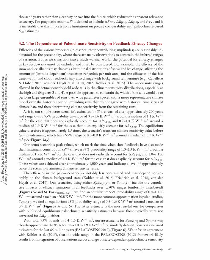
MA10CH11-Rohling ARI 20 October 2017 14:47
thousand years rather than a century or two into the future, which reduces the apparent relevanceto society. For pragmatic reasons, Sa is defined to include �R[T2], �R[SSI], �R[AE], and δ[SO], and itis inevitable that this imposes some limitations on precise comparability with paleoclimate-basedS[sf] estimates.
4.2. The Dependence of Paleoclimate Sensitivity on Feedback Efficacy Changes
Efficacies of the various processes (in essence, their contributing amplitudes) are reasonably un-derstood for the present day, where there are many observations to constrain the inferred rangesof variation. But as we transition into a much warmer world, the potential for efficacy changesin key feedbacks cannot be excluded and must be considered. For example, the efficacy of thesnow and ice albedos may change as latitudinal distributions of snow and ice change, affecting theamount of (latitude-dependent) insolation reflection per unit area, and the efficacies of the fastwater-vapor and cloud feedbacks may also change with background temperature (e.g., Caballero& Huber 2013; von der Heydt et al. 2014, 2016; Kohler et al. 2015). The uncertainty rangesallowed in the actuo-scenario yield wide tails in the climate sensitivity distributions, especially atthe high end (Figures 3 and 4). A possible approach to constrain the width of the tails would be toperform large ensembles of runs over wide parameter spaces with a more representative climatemodel over the historical period, excluding runs that do not agree with historical time series ofclimate data and then determining climate sensitivity from the remaining runs.
As it is, our simple actuo-scenario’s estimates for Sa are reached after approximately 200 yearsand range over a 95% probability envelope of 0.8–1.6 K W−1 m2 around a median of 1.1 K W−1
m2 for the case that does not explicitly account for �R[CFB], and 0.7–1.4 K W−1 m2 around amedian of 1.0 K W−1 m2 for the case that does explicitly account for �R[CFB]. The equilibriumvalue therefore is approximately 1.5 times the scenario’s transient climate sensitivity value beforeδ[SO] involvement, which has a 95% range of 0.5–0.9 K W−1 m2 around a median of 0.7 K W−1
m2 (see Figure 3a,c).Our actuo-scenario’s peak values, which mark the time when slow feedbacks have also made
their maximum contribution (Smax), have a 95% probability range of 1.0–2.3 K W−1 m2 around amedian of 1.5 K W−1 m2 for the case that does not explicitly account for �R[CFB], and 1.0–2.1 KW−1 m2 around a median of 1.4 K W−1 m2 for the case that does explicitly account for �R[CFB].These values are achieved after approximately 1,000 years and indicate a level of approximatelytwice the scenario’s transient climate sensitivity value.
The efficacies in the paleo-scenario are notably less constrained and may depend consid-erably on the climate background state (Kohler et al. 2015, Friedrich et al. 2016, von derHeydt et al. 2016). Our scenarios, using either S[GHG,LI,VG] or S[GHG,LI], include the cumula-tive impacts of efficacy variations in all feedbacks over ±50% ranges (uniformly distributed)(Figures 5c and 6). For S[GHG,LI,VG], we find an equilibrium 95% probability range of 0.4–1.3 KW−1 m2 around a median of 0.8 K W−1 m2. For the more common approximation in paleo-studies,S[GHG,LI], we find an equilibrium 95% probability range of 0.5–1.6 K W−1 m2 around a median of0.9 K W−1 m2 (Figures 5c and 6). The latter estimate is the most useful one for comparisonwith published equilibrium paleoclimate sensitivity estimates because those typically were notcorrected for �R[VG] either.
With total 95% bounds of 0.4–1.6 K W−1 m2, our assessments for S[GHG,LI] and S[GHG,LI,VG]
closely approximate the 95% bounds of 0.3–1.9 K W−1 m2 for similarly defined, observation-basedestimates for the last 65 million years (PALAEOSENS 2012) (Figure 6). We infer, in agreementwith Kohler et al. (2015), that the wide range in the PALAEOSENS (2012) framework likelyresults from integration of observations across a range of state-dependent paleoclimate sensitivity
www.annualreviews.org • Comparing Climate Sensitivity 281
Ann
u. R
ev. M
ar. S
ci. 2
018.
10:2
61-2
88. D
ownl
oade
d fr
om w
ww
.ann
ualr
evie
ws.
org
Acc
ess
prov
ided
by
Aus
tral
ian
Nat
iona
l Uni
vers
ity o
n 06
/03/
19. F
or p
erso
nal u
se o
nly.
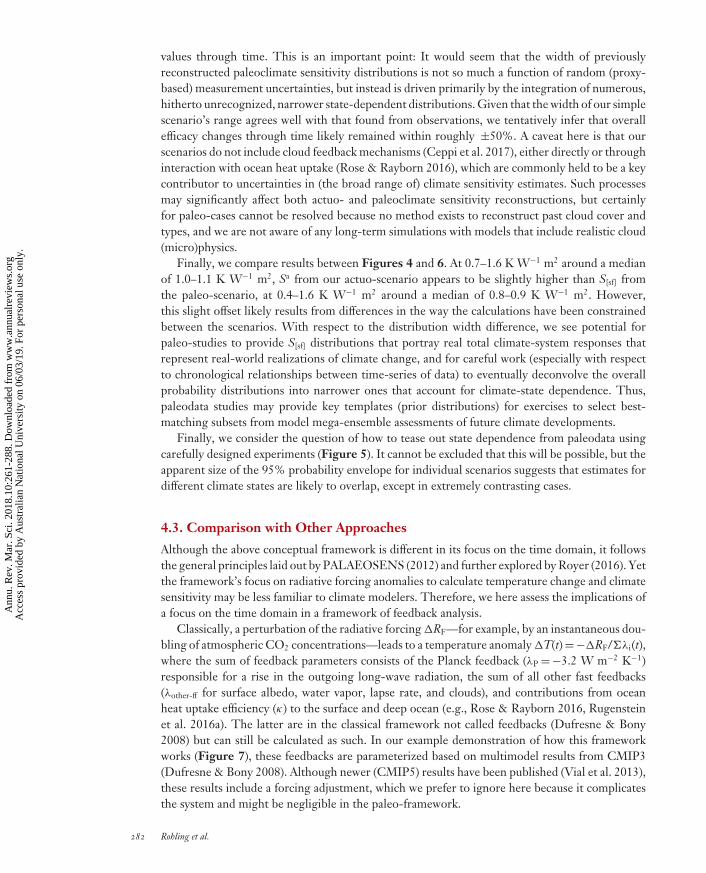
MA10CH11-Rohling ARI 20 October 2017 14:47
values through time. This is an important point: It would seem that the width of previouslyreconstructed paleoclimate sensitivity distributions is not so much a function of random (proxy-based) measurement uncertainties, but instead is driven primarily by the integration of numerous,hitherto unrecognized, narrower state-dependent distributions. Given that the width of our simplescenario’s range agrees well with that found from observations, we tentatively infer that overallefficacy changes through time likely remained within roughly ±50%. A caveat here is that ourscenarios do not include cloud feedback mechanisms (Ceppi et al. 2017), either directly or throughinteraction with ocean heat uptake (Rose & Rayborn 2016), which are commonly held to be a keycontributor to uncertainties in (the broad range of) climate sensitivity estimates. Such processesmay significantly affect both actuo- and paleoclimate sensitivity reconstructions, but certainlyfor paleo-cases cannot be resolved because no method exists to reconstruct past cloud cover andtypes, and we are not aware of any long-term simulations with models that include realistic cloud(micro)physics.
Finally, we compare results between Figures 4 and 6. At 0.7–1.6 K W−1 m2 around a medianof 1.0–1.1 K W−1 m2, Sa from our actuo-scenario appears to be slightly higher than S[sf] fromthe paleo-scenario, at 0.4–1.6 K W−1 m2 around a median of 0.8–0.9 K W−1 m2. However,this slight offset likely results from differences in the way the calculations have been constrainedbetween the scenarios. With respect to the distribution width difference, we see potential forpaleo-studies to provide S[sf] distributions that portray real total climate-system responses thatrepresent real-world realizations of climate change, and for careful work (especially with respectto chronological relationships between time-series of data) to eventually deconvolve the overallprobability distributions into narrower ones that account for climate-state dependence. Thus,paleodata studies may provide key templates (prior distributions) for exercises to select best-matching subsets from model mega-ensemble assessments of future climate developments.
Finally, we consider the question of how to tease out state dependence from paleodata usingcarefully designed experiments (Figure 5). It cannot be excluded that this will be possible, but theapparent size of the 95% probability envelope for individual scenarios suggests that estimates fordifferent climate states are likely to overlap, except in extremely contrasting cases.
4.3. Comparison with Other Approaches
Although the above conceptual framework is different in its focus on the time domain, it followsthe general principles laid out by PALAEOSENS (2012) and further explored by Royer (2016). Yetthe framework’s focus on radiative forcing anomalies to calculate temperature change and climatesensitivity may be less familiar to climate modelers. Therefore, we here assess the implications ofa focus on the time domain in a framework of feedback analysis.
Classically, a perturbation of the radiative forcing �RF—for example, by an instantaneous dou-bling of atmospheric CO2 concentrations—leads to a temperature anomaly �T(t)=−�RF/λi(t),where the sum of feedback parameters consists of the Planck feedback (λP=−3.2 W m−2 K−1)responsible for a rise in the outgoing long-wave radiation, the sum of all other fast feedbacks(λother-ff for surface albedo, water vapor, lapse rate, and clouds), and contributions from oceanheat uptake efficiency (κ) to the surface and deep ocean (e.g., Rose & Rayborn 2016, Rugensteinet al. 2016a). The latter are in the classical framework not called feedbacks (Dufresne & Bony2008) but can still be calculated as such. In our example demonstration of how this frameworkworks (Figure 7), these feedbacks are parameterized based on multimodel results from CMIP3(Dufresne & Bony 2008). Although newer (CMIP5) results have been published (Vial et al. 2013),these results include a forcing adjustment, which we prefer to ignore here because it complicatesthe system and might be negligible in the paleo-framework.
282 Rohling et al.
Ann
u. R
ev. M
ar. S
ci. 2
018.
10:2
61-2
88. D
ownl
oade
d fr
om w
ww
.ann
ualr
evie
ws.
org
Acc
ess
prov
ided
by
Aus
tral
ian
Nat
iona
l Uni
vers
ity o
n 06
/03/
19. F
or p
erso
nal u
se o
nly.
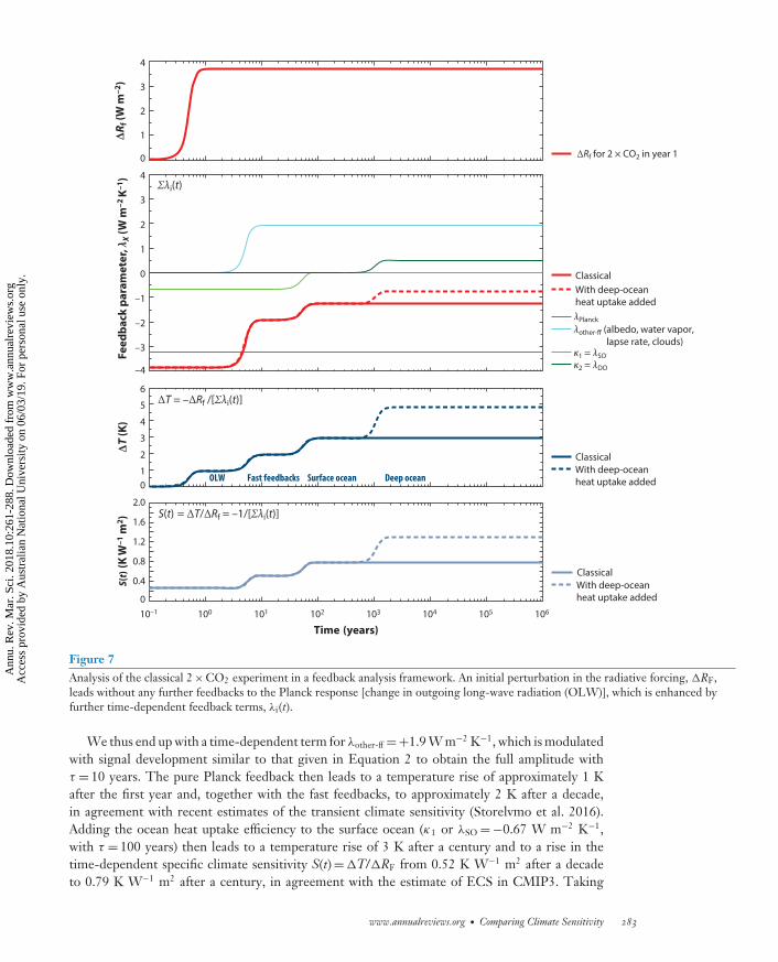
MA10CH11-Rohling ARI 20 October 2017 14:47
–4
–3
–2
–1
0
1
2
3
4
Feed
back
par
amet
er, λ
X (W
m–2
K–1)
10–1 100 101 102 103 104 105 106
Time (years)
ClassicalWith deep-oceanheat uptake added
λother-ff (albedo, water vapor, lapse rate, clouds)κ1 = λSOκ2 = λDO
λPlanck
0
1
2
3
4
ΔRf (
W m
–2)
ΔT (K
)
ΔRf for 2 × CO2 in year 1
01
2
3
4
5
6
ClassicalWith deep-oceanheat uptake added
With deep-oceanheat uptake added
OLW Fast feedbacks Surface ocean Deep ocean
0
0.4
0.8
1.2
1.6
2.0
S(t)
(K W
–1 m
2 ) S(t) = ΔT/ΔRf = –1/[Σλi(t)]
ΔT = –ΔRf /[Σλi(t)]
Classical
Σλi(t)
Figure 7Analysis of the classical 2×CO2 experiment in a feedback analysis framework. An initial perturbation in the radiative forcing, �RF,leads without any further feedbacks to the Planck response [change in outgoing long-wave radiation (OLW)], which is enhanced byfurther time-dependent feedback terms, λi(t).
We thus end up with a time-dependent term for λother-ff=+1.9 W m−2 K−1, which is modulatedwith signal development similar to that given in Equation 2 to obtain the full amplitude withτ = 10 years. The pure Planck feedback then leads to a temperature rise of approximately 1 Kafter the first year and, together with the fast feedbacks, to approximately 2 K after a decade,in agreement with recent estimates of the transient climate sensitivity (Storelvmo et al. 2016).Adding the ocean heat uptake efficiency to the surface ocean (κ1 or λSO=−0.67 W m−2 K−1,with τ = 100 years) then leads to a temperature rise of 3 K after a century and to a rise in thetime-dependent specific climate sensitivity S(t)=�T/�RF from 0.52 K W−1 m2 after a decadeto 0.79 K W−1 m2 after a century, in agreement with the estimate of ECS in CMIP3. Taking
www.annualreviews.org • Comparing Climate Sensitivity 283
Ann
u. R
ev. M
ar. S
ci. 2
018.
10:2
61-2
88. D
ownl
oade
d fr
om w
ww
.ann
ualr
evie
ws.
org
Acc
ess
prov
ided
by
Aus
tral
ian
Nat
iona
l Uni
vers
ity o
n 06
/03/
19. F
or p
erso
nal u
se o
nly.
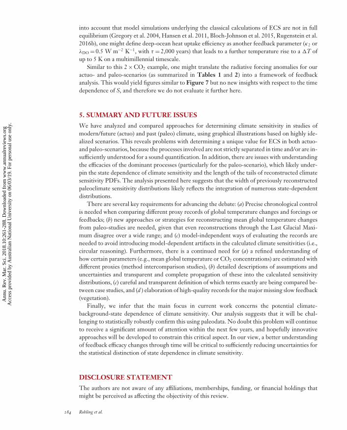
MA10CH11-Rohling ARI 20 October 2017 14:47
into account that model simulations underlying the classical calculations of ECS are not in fullequilibrium (Gregory et al. 2004, Hansen et al. 2011, Bloch-Johnson et al. 2015, Rugenstein et al.2016b), one might define deep-ocean heat uptake efficiency as another feedback parameter (κ2 orλDO= 0.5 W m−2 K−1, with τ = 2,000 years) that leads to a further temperature rise to a �T ofup to 5 K on a multimillennial timescale.
Similar to this 2×CO2 example, one might translate the radiative forcing anomalies for ouractuo- and paleo-scenarios (as summarized in Tables 1 and 2) into a framework of feedbackanalysis. This would yield figures similar to Figure 7 but no new insights with respect to the timedependence of S, and therefore we do not evaluate it further here.
5. SUMMARY AND FUTURE ISSUES
We have analyzed and compared approaches for determining climate sensitivity in studies ofmodern/future (actuo) and past (paleo) climate, using graphical illustrations based on highly ide-alized scenarios. This reveals problems with determining a unique value for ECS in both actuo-and paleo-scenarios, because the processes involved are not strictly separated in time and/or are in-sufficiently understood for a sound quantification. In addition, there are issues with understandingthe efficacies of the dominant processes (particularly for the paleo-scenario), which likely under-pin the state dependence of climate sensitivity and the length of the tails of reconstructed climatesensitivity PDFs. The analysis presented here suggests that the width of previously reconstructedpaleoclimate sensitivity distributions likely reflects the integration of numerous state-dependentdistributions.
There are several key requirements for advancing the debate: (a) Precise chronological controlis needed when comparing different proxy records of global temperature changes and forcings orfeedbacks; (b) new approaches or strategies for reconstructing mean global temperature changesfrom paleo-studies are needed, given that even reconstructions through the Last Glacial Maxi-mum disagree over a wide range; and (c) model-independent ways of evaluating the records areneeded to avoid introducing model-dependent artifacts in the calculated climate sensitivities (i.e.,circular reasoning). Furthermore, there is a continued need for (a) a refined understanding ofhow certain parameters (e.g., mean global temperature or CO2 concentrations) are estimated withdifferent proxies (method intercomparison studies), (b) detailed descriptions of assumptions anduncertainties and transparent and complete propagation of these into the calculated sensitivitydistributions, (c) careful and transparent definition of which terms exactly are being compared be-tween case studies, and (d ) elaboration of high-quality records for the major missing slow feedback(vegetation).
Finally, we infer that the main focus in current work concerns the potential climate-background-state dependence of climate sensitivity. Our analysis suggests that it will be chal-lenging to statistically robustly confirm this using paleodata. No doubt this problem will continueto receive a significant amount of attention within the next few years, and hopefully innovativeapproaches will be developed to constrain this critical aspect. In our view, a better understandingof feedback efficacy changes through time will be critical to sufficiently reducing uncertainties forthe statistical distinction of state dependence in climate sensitivity.
DISCLOSURE STATEMENT
The authors are not aware of any affiliations, memberships, funding, or financial holdings thatmight be perceived as affecting the objectivity of this review.
284 Rohling et al.
Ann
u. R
ev. M
ar. S
ci. 2
018.
10:2
61-2
88. D
ownl
oade
d fr
om w
ww
.ann
ualr
evie
ws.
org
Acc
ess
prov
ided
by
Aus
tral
ian
Nat
iona
l Uni
vers
ity o
n 06
/03/
19. F
or p
erso
nal u
se o
nly.
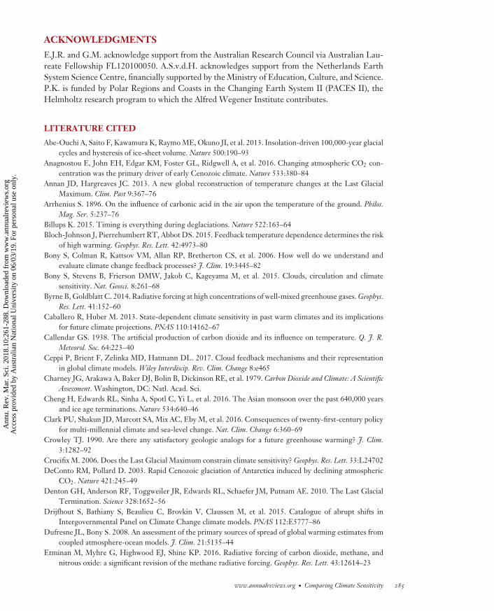
MA10CH11-Rohling ARI 20 October 2017 14:47
ACKNOWLEDGMENTS
E.J.R. and G.M. acknowledge support from the Australian Research Council via Australian Lau-reate Fellowship FL120100050. A.S.v.d.H. acknowledges support from the Netherlands EarthSystem Science Centre, financially supported by the Ministry of Education, Culture, and Science.P.K. is funded by Polar Regions and Coasts in the Changing Earth System II (PACES II), theHelmholtz research program to which the Alfred Wegener Institute contributes.
LITERATURE CITED
Abe-Ouchi A, Saito F, Kawamura K, Raymo ME, Okuno JI, et al. 2013. Insolation-driven 100,000-year glacialcycles and hysteresis of ice-sheet volume. Nature 500:190–93
Anagnostou E, John EH, Edgar KM, Foster GL, Ridgwell A, et al. 2016. Changing atmospheric CO2 con-centration was the primary driver of early Cenozoic climate. Nature 533:380–84
Annan JD, Hargreaves JC. 2013. A new global reconstruction of temperature changes at the Last GlacialMaximum. Clim. Past 9:367–76
Arrhenius S. 1896. On the influence of carbonic acid in the air upon the temperature of the ground. Philos.Mag. Ser. 5:237–76
Billups K. 2015. Timing is everything during deglaciations. Nature 522:163–64Bloch-Johnson J, Pierrehumbert RT, Abbot DS. 2015. Feedback temperature dependence determines the risk
of high warming. Geophys. Res. Lett. 42:4973–80Bony S, Colman R, Kattsov VM, Allan RP, Bretherton CS, et al. 2006. How well do we understand and
evaluate climate change feedback processes? J. Clim. 19:3445–82Bony S, Stevens B, Frierson DMW, Jakob C, Kageyama M, et al. 2015. Clouds, circulation and climate
sensitivity. Nat. Geosci. 8:261–68Byrne B, Goldblatt C. 2014. Radiative forcing at high concentrations of well-mixed greenhouse gases. Geophys.
Res. Lett. 41:152–60Caballero R, Huber M. 2013. State-dependent climate sensitivity in past warm climates and its implications
for future climate projections. PNAS 110:14162–67Callendar GS. 1938. The artificial production of carbon dioxide and its influence on temperature. Q. J. R.
Meteorol. Soc. 64:223–40Ceppi P, Brient F, Zelinka MD, Hatmann DL. 2017. Cloud feedback mechanisms and their representation
in global climate models. Wiley Interdiscip. Rev. Clim. Change 8:e465Charney JG, Arakawa A, Baker DJ, Bolin B, Dickinson RE, et al. 1979. Carbon Dioxide and Climate: A Scientific
Assessment. Washington, DC: Natl. Acad. Sci.Cheng H, Edwards RL, Sinha A, Spotl C, Yi L, et al. 2016. The Asian monsoon over the past 640,000 years
and ice age terminations. Nature 534:640–46Clark PU, Shakun JD, Marcott SA, Mix AC, Eby M, et al. 2016. Consequences of twenty-first-century policy
for multi-millennial climate and sea-level change. Nat. Clim. Change 6:360–69Crowley TJ. 1990. Are there any satisfactory geologic analogs for a future greenhouse warming? J. Clim.
3:1282–92Crucifix M. 2006. Does the Last Glacial Maximum constrain climate sensitivity? Geophys. Res. Lett. 33:L24702DeConto RM, Pollard D. 2003. Rapid Cenozoic glaciation of Antarctica induced by declining atmospheric
CO2. Nature 421:245–49Denton GH, Anderson RF, Toggweiler JR, Edwards RL, Schaefer JM, Putnam AE. 2010. The Last Glacial
Termination. Science 328:1652–56Drijfhout S, Bathiany S, Beaulieu C, Brovkin V, Claussen M, et al. 2015. Catalogue of abrupt shifts in
Intergovernmental Panel on Climate Change climate models. PNAS 112:E5777–86Dufresne JL, Bony S. 2008. An assessment of the primary sources of spread of global warming estimates from
coupled atmosphere-ocean models. J. Clim. 21:5135–44Etminan M, Myhre G, Highwood EJ, Shine KP. 2016. Radiative forcing of carbon dioxide, methane, and
nitrous oxide: a significant revision of the methane radiative forcing. Geophys. Res. Lett. 43:12614–23
www.annualreviews.org • Comparing Climate Sensitivity 285
Ann
u. R
ev. M
ar. S
ci. 2
018.
10:2
61-2
88. D
ownl
oade
d fr
om w
ww
.ann
ualr
evie
ws.
org
Acc
ess
prov
ided
by
Aus
tral
ian
Nat
iona
l Uni
vers
ity o
n 06
/03/
19. F
or p
erso
nal u
se o
nly.
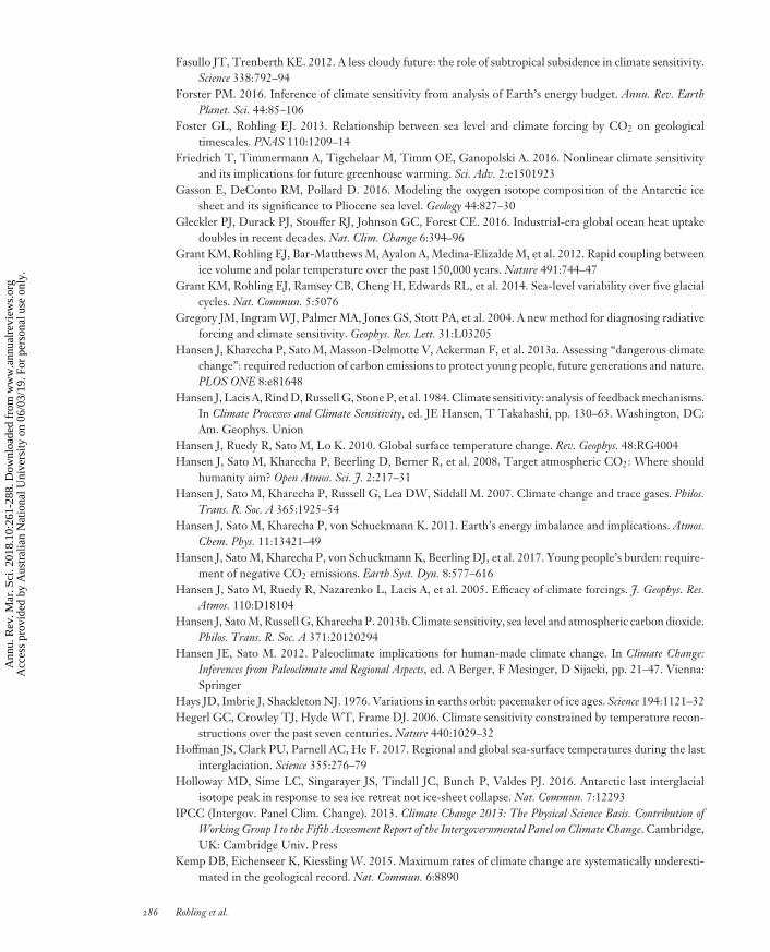
MA10CH11-Rohling ARI 20 October 2017 14:47
Fasullo JT, Trenberth KE. 2012. A less cloudy future: the role of subtropical subsidence in climate sensitivity.Science 338:792–94
Forster PM. 2016. Inference of climate sensitivity from analysis of Earth’s energy budget. Annu. Rev. EarthPlanet. Sci. 44:85–106
Foster GL, Rohling EJ. 2013. Relationship between sea level and climate forcing by CO2 on geologicaltimescales. PNAS 110:1209–14
Friedrich T, Timmermann A, Tigchelaar M, Timm OE, Ganopolski A. 2016. Nonlinear climate sensitivityand its implications for future greenhouse warming. Sci. Adv. 2:e1501923
Gasson E, DeConto RM, Pollard D. 2016. Modeling the oxygen isotope composition of the Antarctic icesheet and its significance to Pliocene sea level. Geology 44:827–30
Gleckler PJ, Durack PJ, Stouffer RJ, Johnson GC, Forest CE. 2016. Industrial-era global ocean heat uptakedoubles in recent decades. Nat. Clim. Change 6:394–96
Grant KM, Rohling EJ, Bar-Matthews M, Ayalon A, Medina-Elizalde M, et al. 2012. Rapid coupling betweenice volume and polar temperature over the past 150,000 years. Nature 491:744–47
Grant KM, Rohling EJ, Ramsey CB, Cheng H, Edwards RL, et al. 2014. Sea-level variability over five glacialcycles. Nat. Commun. 5:5076
Gregory JM, Ingram WJ, Palmer MA, Jones GS, Stott PA, et al. 2004. A new method for diagnosing radiativeforcing and climate sensitivity. Geophys. Res. Lett. 31:L03205
Hansen J, Kharecha P, Sato M, Masson-Delmotte V, Ackerman F, et al. 2013a. Assessing “dangerous climatechange”: required reduction of carbon emissions to protect young people, future generations and nature.PLOS ONE 8:e81648
Hansen J, Lacis A, Rind D, Russell G, Stone P, et al. 1984. Climate sensitivity: analysis of feedback mechanisms.In Climate Processes and Climate Sensitivity, ed. JE Hansen, T Takahashi, pp. 130–63. Washington, DC:Am. Geophys. Union
Hansen J, Ruedy R, Sato M, Lo K. 2010. Global surface temperature change. Rev. Geophys. 48:RG4004Hansen J, Sato M, Kharecha P, Beerling D, Berner R, et al. 2008. Target atmospheric CO2: Where should
humanity aim? Open Atmos. Sci. J. 2:217–31Hansen J, Sato M, Kharecha P, Russell G, Lea DW, Siddall M. 2007. Climate change and trace gases. Philos.
Trans. R. Soc. A 365:1925–54Hansen J, Sato M, Kharecha P, von Schuckmann K. 2011. Earth’s energy imbalance and implications. Atmos.
Chem. Phys. 11:13421–49Hansen J, Sato M, Kharecha P, von Schuckmann K, Beerling DJ, et al. 2017. Young people’s burden: require-
ment of negative CO2 emissions. Earth Syst. Dyn. 8:577–616Hansen J, Sato M, Ruedy R, Nazarenko L, Lacis A, et al. 2005. Efficacy of climate forcings. J. Geophys. Res.
Atmos. 110:D18104Hansen J, Sato M, Russell G, Kharecha P. 2013b. Climate sensitivity, sea level and atmospheric carbon dioxide.
Philos. Trans. R. Soc. A 371:20120294Hansen JE, Sato M. 2012. Paleoclimate implications for human-made climate change. In Climate Change:
Inferences from Paleoclimate and Regional Aspects, ed. A Berger, F Mesinger, D Sijacki, pp. 21–47. Vienna:Springer
Hays JD, Imbrie J, Shackleton NJ. 1976. Variations in earths orbit: pacemaker of ice ages. Science 194:1121–32Hegerl GC, Crowley TJ, Hyde WT, Frame DJ. 2006. Climate sensitivity constrained by temperature recon-
structions over the past seven centuries. Nature 440:1029–32Hoffman JS, Clark PU, Parnell AC, He F. 2017. Regional and global sea-surface temperatures during the last
interglaciation. Science 355:276–79Holloway MD, Sime LC, Singarayer JS, Tindall JC, Bunch P, Valdes PJ. 2016. Antarctic last interglacial
isotope peak in response to sea ice retreat not ice-sheet collapse. Nat. Commun. 7:12293IPCC (Intergov. Panel Clim. Change). 2013. Climate Change 2013: The Physical Science Basis. Contribution of
Working Group I to the Fifth Assessment Report of the Intergovernmental Panel on Climate Change. Cambridge,UK: Cambridge Univ. Press
Kemp DB, Eichenseer K, Kiessling W. 2015. Maximum rates of climate change are systematically underesti-mated in the geological record. Nat. Commun. 6:8890
286 Rohling et al.
Ann
u. R
ev. M
ar. S
ci. 2
018.
10:2
61-2
88. D
ownl
oade
d fr
om w
ww
.ann
ualr
evie
ws.
org
Acc
ess
prov
ided
by
Aus
tral
ian
Nat
iona
l Uni
vers
ity o
n 06
/03/
19. F
or p
erso
nal u
se o
nly.
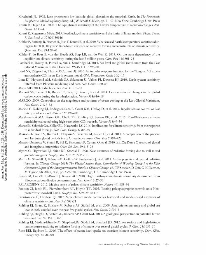
MA10CH11-Rohling ARI 20 October 2017 14:47
Kirschvink JL. 1992. Late proterozoic low latitude global glaciation: the snowball Earth. In The ProterozoicBiosphere: A Multidisciplinary Study, ed. JW Schoff, C Klein, pp. 51–52. New York: Cambridge Univ. Press
Knutti R, Hegerl GC. 2008. The equilibrium sensitivity of the Earth’s temperature to radiation changes. Nat.Geosci. 1:735–43
Knutti R, Rugenstein MAA. 2015. Feedbacks, climate sensitivity and the limits of linear models. Philos. Trans.R. Soc. Lond. A 373:20150146
Kohler P, Bintanja R, Fischer H, Joos F, Knutti R, et al. 2010. What caused Earth’s temperature variations dur-ing the last 800,000 years? Data-based evidence on radiative forcing and constraints on climate sensitivity.Quat. Sci. Rev. 29:129–45
Kohler P, de Boer B, von der Heydt AS, Stap LB, van de Wal R. 2015. On the state dependency of theequilibrium climate sensitivity during the last 5 million years. Clim. Past 11:1801–23
Lambeck K, Rouby H, Purcell A, Sun Y, Sambridge M. 2014. Sea level and global ice volumes from the LastGlacial Maximum to the Holocene. PNAS 111:15296–303
Lord NS, Ridgwell A, Thorne MC, Lunt DJ. 2016. An impulse response function for the “long tail” of excessatmospheric CO2 in an Earth system model. Glob. Biogeochem. Cycles 30:2–17
Lunt DJ, Haywood AM, Schmidt GA, Salzmann U, Valdes PJ, Dowsett HJ. 2010. Earth system sensitivityinferred from Pliocene modelling and data. Nat. Geosci. 3:60–64
Mann ME. 2014. False hope. Sci. Am. 310:78–81Marcott SA, Bauska TK, Buizert C, Steig EJ, Rosen JL, et al. 2014. Centennial-scale changes in the global
carbon cycle during the last deglaciation. Nature 514:616–19MARGO. 2009. Constraints on the magnitude and patterns of ocean cooling at the Last Glacial Maximum.
Nat. Geosci. 2:127–32Marino G, Rohling EJ, Rodriguez-Sanz L, Grant KM, Heslop D, et al. 2015. Bipolar seesaw control on last
interglacial sea level. Nature 522:197–201Martınez-Botı MA, Foster GL, Chalk TB, Rohling EJ, Sexton PF, et al. 2015. Plio-Pleistocene climate
sensitivity evaluated using high-resolution CO2 records. Nature 518:49–54Marvel K, Schmidt GA, Miller RL, Nazarenko LS. 2016. Implications for climate sensitivity from the response
to individual forcings. Nat. Clim. Change 6:386–89Masson-Delmotte V, Buiron D, Ekaykin A, Frezzotti M, Gallee H, et al. 2011. A comparison of the present
and last interglacial periods in six Antarctic ice cores. Clim. Past 7:397–423Masson-Delmotte V, Stenni B, Pol K, Braconnot P, Cattani O, et al. 2010. EPICA Dome C record of glacial
and interglacial intensities. Quat. Sci. Rev. 29:113–28Myhre G, Highwood EJ, Shine KP, Stordal F. 1998. New estimates of radiative forcing due to well mixed
greenhouse gases. Geophys. Res. Lett. 25:2715–18Myhre G, Shindell D, Breon F-M, Collins W, Fuglestvedt J, et al. 2013. Anthropogenic and natural radiative
forcing. In Climate Change 2013: The Physical Science Basis. Contribution of Working Group I to the FifthAssessment Report of the Intergovernmental Panel on Climate Change, ed. TF Stocker, D Qin, G-K Plattner,M Tignor, SK Allen, et al, pp. 659–740. Cambridge, UK: Cambridge Univ. Press
Pagani M, Liu ZH, LaRiviere J, Ravelo AC. 2010. High Earth-system climate sensitivity determined fromPliocene carbon dioxide concentrations. Nat. Geosci. 3:27–30
PALAEOSENS. 2012. Making sense of palaeoclimate sensitivity. Nature 491:683–91Poulsen CJ, Jacob RL, Pierrehumbert RT, Huynh TT. 2002. Testing paleogeographic controls on a Neo-
proterozoic snowball Earth. Geophys. Res. Lett. 29:10-1–4Proistosescu C, Huybers PJ. 2017. Slow climate mode reconciles historical and model-based estimates of
climate sensitivity. Sci. Adv. 3:e1602821Rohling EJ, Grant K, Bolshaw M, Roberts AP, Siddall M, et al. 2009. Antarctic temperature and global sea
level closely coupled over the past five glacial cycles. Nat. Geosci. 2:500–4Rohling EJ, Haigh ID, Foster GL, Roberts AP, Grant KM. 2013. A geological perspective on potential future
sea-level rise. Sci. Rep. 3:3461Rohling EJ, Medina-Elizalde M, Shepherd JG, Siddall M, Stanford JD. 2012. Sea surface and high-latitude
temperature sensitivity to radiative forcing of climate over several glacial cycles. J. Clim. 25:1635–56Rose BEJ, Rayborn L. 2016. The effects of ocean heat uptake on transient climate sensitivity. Curr. Clim.
Change Rep. 2:190–201
www.annualreviews.org • Comparing Climate Sensitivity 287
Ann
u. R
ev. M
ar. S
ci. 2
018.
10:2
61-2
88. D
ownl
oade
d fr
om w
ww
.ann
ualr
evie
ws.
org
Acc
ess
prov
ided
by
Aus
tral
ian
Nat
iona
l Uni
vers
ity o
n 06
/03/
19. F
or p
erso
nal u
se o
nly.
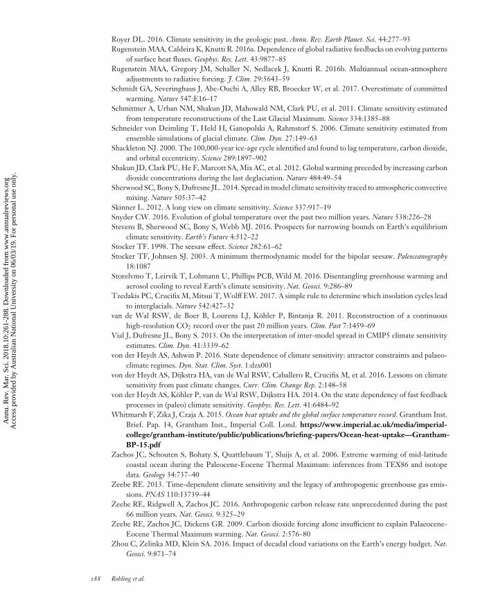
MA10CH11-Rohling ARI 20 October 2017 14:47
Royer DL. 2016. Climate sensitivity in the geologic past. Annu. Rev. Earth Planet. Sci. 44:277–93Rugenstein MAA, Caldeira K, Knutti R. 2016a. Dependence of global radiative feedbacks on evolving patterns
of surface heat fluxes. Geophys. Res. Lett. 43:9877–85Rugenstein MAA, Gregory JM, Schaller N, Sedlacek J, Knutti R. 2016b. Multiannual ocean-atmosphere
adjustments to radiative forcing. J. Clim. 29:5643–59Schmidt GA, Severinghaus J, Abe-Ouchi A, Alley RB, Broecker W, et al. 2017. Overestimate of committed
warming. Nature 547:E16–17Schmittner A, Urban NM, Shakun JD, Mahowald NM, Clark PU, et al. 2011. Climate sensitivity estimated
from temperature reconstructions of the Last Glacial Maximum. Science 334:1385–88Schneider von Deimling T, Held H, Ganopolski A, Rahmstorf S. 2006. Climate sensitivity estimated from
ensemble simulations of glacial climate. Clim. Dyn. 27:149–63Shackleton NJ. 2000. The 100,000-year ice-age cycle identified and found to lag temperature, carbon dioxide,
and orbital eccentricity. Science 289:1897–902Shakun JD, Clark PU, He F, Marcott SA, Mix AC, et al. 2012. Global warming preceded by increasing carbon
dioxide concentrations during the last deglaciation. Nature 484:49–54Sherwood SC, Bony S, Dufresne JL. 2014. Spread in model climate sensitivity traced to atmospheric convective
mixing. Nature 505:37–42Skinner L. 2012. A long view on climate sensitivity. Science 337:917–19Snyder CW. 2016. Evolution of global temperature over the past two million years. Nature 538:226–28Stevens B, Sherwood SC, Bony S, Webb MJ. 2016. Prospects for narrowing bounds on Earth’s equilibrium
climate sensitivity. Earth’s Future 4:512–22Stocker TF. 1998. The seesaw effect. Science 282:61–62Stocker TF, Johnsen SJ. 2003. A minimum thermodynamic model for the bipolar seesaw. Paleoceanography
18:1087Storelvmo T, Leirvik T, Lohmann U, Phillips PCB, Wild M. 2016. Disentangling greenhouse warming and
aerosol cooling to reveal Earth’s climate sensitivity. Nat. Geosci. 9:286–89Tzedakis PC, Crucifix M, Mitsui T, Wolff EW. 2017. A simple rule to determine which insolation cycles lead
to interglacials. Nature 542:427–32van de Wal RSW, de Boer B, Lourens LJ, Kohler P, Bintanja R. 2011. Reconstruction of a continuous
high-resolution CO2 record over the past 20 million years. Clim. Past 7:1459–69Vial J, Dufresne JL, Bony S. 2013. On the interpretation of inter-model spread in CMIP5 climate sensitivity
estimates. Clim. Dyn. 41:3339–62von der Heydt AS, Ashwin P. 2016. State dependence of climate sensitivity: attractor constraints and palaeo-
climate regimes. Dyn. Stat. Clim. Syst. 1:dzx001von der Heydt AS, Dijkstra HA, van de Wal RSW, Caballero R, Crucifix M, et al. 2016. Lessons on climate
sensitivity from past climate changes. Curr. Clim. Change Rep. 2:148–58von der Heydt AS, Kohler P, van de Wal RSW, Dijkstra HA. 2014. On the state dependency of fast feedback
processes in (paleo) climate sensitivity. Geophys. Res. Lett. 41:6484–92Whitmarsh F, Zika J, Czaja A. 2015. Ocean heat uptake and the global surface temperature record. Grantham Inst.
Brief. Pap. 14, Grantham Inst., Imperial Coll. Lond. https://www.imperial.ac.uk/media/imperial-college/grantham-institute/public/publications/briefing-papers/Ocean-heat-uptake—Grantham-BP-15.pdf
Zachos JC, Schouten S, Bohaty S, Quattlebaum T, Sluijs A, et al. 2006. Extreme warming of mid-latitudecoastal ocean during the Paleocene-Eocene Thermal Maximum: inferences from TEX86 and isotopedata. Geology 34:737–40
Zeebe RE. 2013. Time-dependent climate sensitivity and the legacy of anthropogenic greenhouse gas emis-sions. PNAS 110:13739–44
Zeebe RE, Ridgwell A, Zachos JC. 2016. Anthropogenic carbon release rate unprecedented during the past66 million years. Nat. Geosci. 9:325–29
Zeebe RE, Zachos JC, Dickens GR. 2009. Carbon dioxide forcing alone insufficient to explain Palaeocene-Eocene Thermal Maximum warming. Nat. Geosci. 2:576–80
Zhou C, Zelinka MD, Klein SA. 2016. Impact of decadal cloud variations on the Earth’s energy budget. Nat.Geosci. 9:871–74
288 Rohling et al.
Ann
u. R
ev. M
ar. S
ci. 2
018.
10:2
61-2
88. D
ownl
oade
d fr
om w
ww
.ann
ualr
evie
ws.
org
Acc
ess
prov
ided
by
Aus
tral
ian
Nat
iona
l Uni
vers
ity o
n 06
/03/
19. F
or p
erso
nal u
se o
nly.
MA10_TOC ARI 10 October 2017 13:21
Annual Review ofMarine Science
Volume 10, 2018
Contents
A Biogeochemical Oceanographer at Sea: My Life with Nitrogenand a Nod to SilicaRichard C. Dugdale � � � � � � � � � � � � � � � � � � � � � � � � � � � � � � � � � � � � � � � � � � � � � � � � � � � � � � � � � � � � � � � � � � � � � � � � � � � � 1
Applying Movement Ecology to Marine Animals with ComplexLife CyclesRichard M. Allen, Anna Metaxas, and Paul V.R. Snelgrove � � � � � � � � � � � � � � � � � � � � � � � � � � � � � � �19
Ecological Stoichiometry of Ocean PlanktonAllison R. Moreno and Adam C. Martiny � � � � � � � � � � � � � � � � � � � � � � � � � � � � � � � � � � � � � � � � � � � � � � � � � � �43
The Ecology, Biogeochemistry, and Optical Propertiesof CoccolithophoresWilliam M. Balch � � � � � � � � � � � � � � � � � � � � � � � � � � � � � � � � � � � � � � � � � � � � � � � � � � � � � � � � � � � � � � � � � � � � � � � � � � � � �71
A Satellite-Based Lagrangian View on Phytoplankton DynamicsYoav Lehahn, Francesco d’Ovidio, and Ilan Koren � � � � � � � � � � � � � � � � � � � � � � � � � � � � � � � � � � � � � � � � � �99
Spaceborne Lidar in the Study of Marine SystemsChris A. Hostetler, Michael J. Behrenfeld, Yongxiang Hu, Johnathan W. Hair,
and Jennifer A. Schulien � � � � � � � � � � � � � � � � � � � � � � � � � � � � � � � � � � � � � � � � � � � � � � � � � � � � � � � � � � � � � � � � � 121
Remote Sensing Tropical Coral Reefs: The View from AboveSam J. Purkis � � � � � � � � � � � � � � � � � � � � � � � � � � � � � � � � � � � � � � � � � � � � � � � � � � � � � � � � � � � � � � � � � � � � � � � � � � � � � � � � 149
How Do Marine Pelagic Species Respond to Climate Change?Theories and ObservationsGregory Beaugrand and Richard R. Kirby � � � � � � � � � � � � � � � � � � � � � � � � � � � � � � � � � � � � � � � � � � � � � � � � � 169
Improving Marine Ecosystem Models with Biochemical TracersHeidi R. Pethybridge, C. Anela Choy, Jeffrey J. Polovina, and Elizabeth A. Fulton � � � � 199
Manifestation, Drivers, and Emergence of Open Ocean DeoxygenationLisa A. Levin � � � � � � � � � � � � � � � � � � � � � � � � � � � � � � � � � � � � � � � � � � � � � � � � � � � � � � � � � � � � � � � � � � � � � � � � � � � � � � � � 229
Ann
u. R
ev. M
ar. S
ci. 2
018.
10:2
61-2
88. D
ownl
oade
d fr
om w
ww
.ann
ualr
evie
ws.
org
Acc
ess
prov
ided
by
Aus
tral
ian
Nat
iona
l Uni
vers
ity o
n 06
/03/
19. F
or p
erso
nal u
se o
nly.
MA10_TOC ARI 10 October 2017 13:21
Comparing Climate Sensitivity, Past and PresentEelco J. Rohling, Gianluca Marino, Gavin L. Foster, Philip A. Goodwin,
Anna S. von der Heydt, and Peter Kohler � � � � � � � � � � � � � � � � � � � � � � � � � � � � � � � � � � � � � � � � � � � � � � 261
Marine Aerosols and CloudsSarah D. Brooks and Daniel C.O. Thornton � � � � � � � � � � � � � � � � � � � � � � � � � � � � � � � � � � � � � � � � � � � � � � 289
Progress in Deciphering the Controls on the Geochemistry of Fluidsin Seafloor Hydrothermal SystemsSusan E. Humphris and Frieder Klein � � � � � � � � � � � � � � � � � � � � � � � � � � � � � � � � � � � � � � � � � � � � � � � � � � � � � 315
Planktonic Subsidies to Surf-Zone and Intertidal CommunitiesSteven G. Morgan, Alan L. Shanks, Jamie H. MacMahan,
Ad J.H.M. Reniers, and Falk Feddersen � � � � � � � � � � � � � � � � � � � � � � � � � � � � � � � � � � � � � � � � � � � � � � � � 345
Sediment Trapping in EstuariesHans Burchard, Henk M. Schuttelaars, and David K. Ralston � � � � � � � � � � � � � � � � � � � � � � � � � � 371
The Bottom Boundary LayerJohn H. Trowbridge and Steven J. Lentz � � � � � � � � � � � � � � � � � � � � � � � � � � � � � � � � � � � � � � � � � � � � � � � � � � 397
The Fate and Impact of Internal Waves in Nearshore EcosystemsC.B. Woodson � � � � � � � � � � � � � � � � � � � � � � � � � � � � � � � � � � � � � � � � � � � � � � � � � � � � � � � � � � � � � � � � � � � � � � � � � � � � � � � � 421
Mixing Efficiency in the OceanM.C. Gregg, E.A. D’Asaro, J.J. Riley, and E. Kunze � � � � � � � � � � � � � � � � � � � � � � � � � � � � � � � � � � � � 443
The Recent Atlantic Cold Anomaly: Causes, Consequences, andRelated PhenomenaSimon A. Josey, Joel J.-M. Hirschi, Bablu Sinha, Aurelie Duchez,
Jeremy P. Grist, and Robert Marsh � � � � � � � � � � � � � � � � � � � � � � � � � � � � � � � � � � � � � � � � � � � � � � � � � � � � � 475
A Synoptic View of the Ventilation and Circulation of AntarcticBottom Water from Chlorofluorocarbons and Natural TracersSarah G. Purkey, William M. Smethie Jr., Geoffrey Gebbie,
Arnold L. Gordon, Rolf E. Sonnerup, Mark J. Warner, and John L. Bullister � � � � � � 503
Errata
An online log of corrections to Annual Review of Marine Science articles may be found athttp://www.annualreviews.org/errata/marine
Ann
u. R
ev. M
ar. S
ci. 2
018.
10:2
61-2
88. D
ownl
oade
d fr
om w
ww
.ann
ualr
evie
ws.
org
Acc
ess
prov
ided
by
Aus
tral
ian
Nat
iona
l Uni
vers
ity o
n 06
/03/
19. F
or p
erso
nal u
se o
nly.