Embed Size (px)
Citation preview
The Evolution of Climate Sensitivity and Climate Feedbacks in theCommunity Atmosphere Model
A. GETTELMAN AND J. E. KAY
National Center for Atmospheric Research,* Boulder, Colorado
K. M. SHELL
Oregon State University, Corvallis, Oregon
(Manuscript received 8 April 2011, in final form 26 August 2011)
ABSTRACT
The major evolution of the National Center for Atmospheric Research Community Atmosphere Model
(CAM) is used to diagnose climate feedbacks, understand how climate feedbacks change with different
physical parameterizations, and identify the processes and regions that determine climate sensitivity. In the
evolution of CAM from version 4 to version 5, the water vapor, temperature, surface albedo, and lapse rate
feedbacks are remarkably stable across changes to the physical parameterization suite. However, the climate
sensitivity increases from 3.2 K in CAM4 to 4.0 K in CAM5. The difference is mostly due to (i) more positive
cloud feedbacks and (ii) higher CO2 radiative forcing in CAM5. The intermodel differences in cloud feedbacks
are largest in the tropical trade cumulus regime and in the midlatitude storm tracks. The subtropical stratocu-
mulus regions do not contribute strongly to climate feedbacks owing to their small area coverage. A ‘‘modified
Cess’’ configuration for atmosphere-only model experiments is shown to reproduce slab ocean model results.
Several parameterizations contribute to changes in tropical cloud feedbacks between CAM4 and CAM5, but the
new shallow convection scheme causes the largest midlatitude feedback differences and the largest change in
climate sensitivity. Simulations with greater cloud forcing in the mean state have lower climate sensitivity. This
work provides a methodology for further analysis of climate sensitivity across models and a framework for
targeted comparisons with observations that can help constrain climate sensitivity to radiative forcing.
1. Introduction
The earth’s climate system is being perturbed by an-
thropogenic radiative forcing. In addition to direct ra-
diative forcing of the system (e.g., from anthropogenic
greenhouse gases), the responses to radiative forcing
(surface and atmospheric temperature changes) cause
feedbacks within the system that amplify or damp the
changes (Schneider 1972; Cess et al. 1990; Bony et al.
2006). Increases in temperature allow the specific hu-
midity to increase, which increases the greenhouse effect
due to water vapor (the water vapor feedback). Melting
of snow or sea ice lowers the surface albedo, resulting in
more absorption of solar radiation (the surface albedo
feedback). Increases in surface and atmospheric tem-
perature cause more emission to space, a cooling effect
(temperature feedbacks). Clouds exert complex feed-
backs due to their opposite shortwave and longwave
effects. Clouds reflect shortwave radiation to space,
cooling the planet, but absorb longwave radiation and
emit at cooler temperatures, causing warming. Low
clouds cool and high clouds warm, with the balance of
effects being a net cooling (Stephens 2005). Changes to
cloud amount, location, and radiative properties (e.g.,
optical depth) can exert feedbacks on the system.
Any of these feedbacks may significantly alter the
magnitude of the response to radiative forcing. The water
vapor feedback, for example, is large and positive (Held
and Soden 2000). While it is straightforward to calculate
the direct radiative forcing, the feedback response to that
* The National Center for Atmospheric Research is sponsored
by the National Science Foundation.
Corresponding author address: A. Gettelman, National Center
for Atmospheric Research, 1850 Table Mesa Dr., Boulder, CO,
80305.
E-mail: [email protected]
1 MARCH 2012 G E T T E L M A N E T A L . 1453
DOI: 10.1175/JCLI-D-11-00197.1
� 2012 American Meteorological Society
forcing is a complex process to measure and understand.
Although there are many physical, chemical, biological,
and geological feedbacks that operate on a range of time
scales, here we focus on the water vapor, lapse rate/
temperature, surface albedo, and cloud feedbacks, which
are responsible for much of the uncertainty in future
climate projections of the next 100 years (Bony et al.
2006; Solomon et al. 2007). Remaining uncertainties
stem from ocean heat uptake, anthropogenic emissions,
and carbon cycle changes.
Many authors have decomposed and assessed the rel-
ative importance of feedbacks using different methods.
Cess et al. (1990, 1996) used simplified perturbation ex-
periments with uniform 62-K sea surface temperature
(SST) changes under July conditions (known as ‘‘Cess’’
experiments) to diagnose cloud radiative feedbacks.
More comprehensive feedback calculations were per-
formed by Colman (2003), who decomposed feedbacks
into different components such as water vapor, temper-
ature, albedo, and clouds and found a negative across-
model correlation between water vapor and lapse rate
feedbacks. Colman (2003) found agreement between
the Cess experiments and calculations using the partial
radiative perturbation (PRP) technique of Wetherald
and Manabe (1988). Senior and Mitchell (1993) and
Ringer et al. (2006) found large differences between
assessments of feedbacks from either fully coupled or
slab ocean models and Cess experiments. Soden and
Held (2006) recently performed feedback calculations
using a radiative response (or kernel) method. Soden
et al. (2008) showed that the kernel method yielded
results equivalent to full PRP calculations.
Cess et al. (1990) were among the first to report that
cloud feedbacks explain most intermodel differences in
climate feedbacks. This is reiterated in a recent review
(Stephens 2005). Bony et al. (2004) separated cloud
forcing into dynamic and thermodynamic components,
showing that the trade cumulus (moderate subsidence)
regime was most important for cloud feedback. Bony
and Dufresne (2005) found the biggest spread in model
projections of cloud feedback in regions of moderate
subsidence with trade cumulus clouds. Webb et al. (2006)
confirmed that cloud feedbacks were the major source
of spread between models, that low-cloud feedbacks
were at least half of the signal, and that they were not
confined to tropical low cloud (stratocumulus) re-
gions. Medeiros et al. (2008) used aquaplanet experi-
ments and also found that shallow (or trade) cumulus
regimes were most important for cloud feedback.
Williams and Webb (2009) used a clustering method
and noted that regions with low cloud provided the
largest variance in model cloud feedback estimates.
Thus, there is consensus that cloud feedbacks (and
especially shortwave cloud feedback associated with
trade cumulus clouds) are critical for understanding
climate sensitivity.
This work uses radiative kernels to analyze climate
sensitivity and climate feedbacks in two recent versions
of the National Center for Atmospheric Research
(NCAR) general circulation model (GCM), the Com-
munity Atmospheric Model, versions 4 and 5 (CAM4
and CAM5). CAM is the atmospheric component of the
Community Earth System Model (CESM). Shell et al.
(2008) analyzed feedbacks in an earlier version of CAM
using radiative kernels, and Soden et al. (2008) looked at
global feedbacks in a suite of models using radiative
kernels. We aim to document the climate sensitivity and
climate feedbacks in CAM and how they have changed,
as well as to understand what regions, regimes and,
processes are responsible for these feedbacks. We also
provide a framework that can be used generally for
future model analyses and comparisons.
Our methods are described in section 2. We describe
the model formulations and experiments in section 3
present results in section 4. Sensitivity tests are performed
in section 5, a discussion is in section 6, and conclusions
are in section 7.
2. Methodology
We apply radiative kernels calculated offline to the
climate response in doubled CO2 experiments with at-
mospheric GCMs coupled to slab ocean models (SOMs).
In CESM, SOM experiments yield results very similar
to atmospheric models coupled to a full dynamic ocean
(Bitz et al. 2012). For feedbacks attributed to atmo-
spheric physical parameterizations, the same feedbacks
found in the SOM runs can be diagnosed with stand-alone
atmosphere model SST perturbation experiments. We
then use these experiments to better understand the most
critical feedback processes and regimes, which turn out
to be related to clouds.
When the earth’s energy budget is modified, the planet
warms or cools to balance the imposed forcing G and
return the top-of-atmosphere (TOA) energy imbalance
H to zero. At a given time,
H 5 G 2 D(F 2 Q) 5 G 1 DR. (1)
The sign convention is such that a positive forcing G
corresponds to a warming effect. The forcing can be
balanced by an increase in outgoing longwave radiation
(F; positive values indicate a cooling effect) or a decrease
in absorbed solar radiation (Q; positive values indicate
a warming effect) due to the climate response. Thus DR is
the change in net (shortwave minus longwave) TOA (or
1454 J O U R N A L O F C L I M A T E VOLUME 25
top of model in this case) radiation caused by the climate
response. In equilibrium, H 5 0, so G 5 2DR 5 D(F 2 Q).
The climate sensitivity g determines how much the cli-
mate, represented by the global average above-surface
temperature Tas, needs to change for the TOA fluxes to
return to equilibrium:
G 5D(F 2 Q)
DTas
DTas 5 2lDTas, (2)
where l is the feedback parameter in units of watts per
square meter per kelvin and g 5 2G/l (K) is the climate
sensitivity to a forcing G.
Following Zhang et al. (1994), we assume that, to first
order, the total feedback parameter l is the sum of water
vapor q, surface temperature Ts, atmospheric temperature
Ta, surface albedo a, and cloud C feedback parameters:
l 5 lTs
1 lTa
1 lq 1 lC 1 la
1 NT, (3)
where the nonlinear terms NT are less than 10% (Shell
et al. 2008) and each parameter corresponds to the
change in TOA radiation [DR 5 D(Q 2 F)] solely due to
the change in that feedback variable in response to a 1-K
increase in global average surface air temperature (DTas 5
1 K). The temperature feedback lTacan be separated into
components owing to a uniform change in atmospheric
temperature with height, the ‘‘Planck’’ feedback lTp
, and
a feedback due to changes in temperature lapse rate
lLR. Thus, in Eq. (3), lTa
5 lTp
1 lLR
.
The radiative kernel technique (Soden et al. 2008;
Shell et al. 2008) factors the feedback parameter for
each climate variable X into two parts by approximating
the change in (Q 2 F) in response to DX as linear around
some base state. The quantity [›(Q 2 F)/›X] 5 (›R/›X)
is the radiative kernel, the change in TOA fluxes due to
a standard change in a physical climate variable (the
adjoint radiative response). It is calculated using an off-
line radiative transfer model and depends on the radi-
ative transfer code, as well as the base state, where the
base state—and the kernel—are a function of space and
time. The climate response of the variable is (dX/dTas).
The climate response is calculated discretely as (DX/DTas),
where DX is the difference in the climate variable X be-
tween the experimental and control GCM simulations.
Then the climate feedback parameter lX is
lX(x, y, [z], t) 5›R
›X
DX
DTas
; (4)
lX is computed for every horizontal grid point (x, y) and
altitude (z) for all X except Ts and a, for every month of
the year (t). Where the feedback is not single level, the
contributions in the vertical (z) can be summed to get
the net DH for each column. For the water vapor feed-
back, we use lnq as the feedback variable because it scales
well with the radiation. Lapse rate feedback parameters
are determined from the atmospheric temperature kernel
and the departure of the atmospheric temperature change
from the above-surface temperature change (DTas).
Because cloud feedbacks are affected by the state of
the climate system, to diagnose cloud feedback we use the
change in cloud radiative forcing (CRF) (Ramanathan
et al. 1989), adjusted to remove the effects of changing
noncloud fields. CRF is the difference between the all-sky
TOA flux (all) and the clear-sky TOA flux (clr)—the
TOA flux the atmospheric column would have if clouds
were removed but all other variables remained the same.
For the longwave (LW) CRFLW 5 Fall 2 Fclr, and for the
shortwave (SW) CRFSW 5 Qall 2 Qclr so that CRF 5
CRFLW 1 CRFSW. The cloud feedback (CF) can be es-
timated by taking DCRF/DTas.
However, DCRF can be influenced by changes in non-
cloud variables (Zhang et al. 1994; Colman 2003; Soden
et al. 2004). For example, if the surface albedo changes,
CRF will change, even if clouds remain the same, because
Rclr changes. We can thus subtract contributions to DCRF
due to water vapor, temperature, surface albedo, and
forcing (CO2) changes to obtain the adjusted DCRF.
The adjusted cloud feedback (ACF) is the adjusted
DCRF divided by the global average near-surface tem-
perature change (DTas). Cloud feedbacks can also be
decomposed into SW and LW components (ASCF and
ALCF, respectively).
The radiative kernels used in this study were calculated
offline with CAM, version 3 (CAM3) (Shell et al. 2008).
Soden et al. (2008) have shown globally that the radiative
kernels calculated with different models produce similar
results, so the use of CAM3 kernels is appropriate.
Finally, we will calculate the climate sensitivity g for
the different runs. First, we calculate an effective feed-
back parameter leff using the total change in forcing and
TOA energy imbalance between two runs with different
surface temperatures and CO2 concentrations:
leff 5 2(GCO22 H)/DTas, (5)
where GCO2is the radiative forcing. For doubling CO2
from 280 to 560 ppm by volume (ppmv), GCO25 3:5 or
3.8 W m22, depending on the model version (see section
6), and H is the change in TOA imbalance. The effective
climate sensitivity (geff) is then geff
5 2GCO2
/leff
. For
an equilibrium state (H 5 0), this reduces to DTas. The
method allows an estimate of g from runs that are out of
balance (H 6¼ 0). Below we show that, for the same
model code in equilibrium (a slab ocean model) and out
1 MARCH 2012 G E T T E L M A N E T A L . 1455
of balance (specified SST formulation), geff ’ g. This
method is conceptually similar to the regression slope
method of Gregory et al. (2004).
Feedbacks with vertical structure are integrated over
the troposphere. Here the troposphere is defined as the
region with pressures higher than 100 hPa. We use this
convention throughout the paper except for lapse rate
feedbacks where we use pressures higher than 300 hPa
poleward of 308 latitude and pressure higher than 100 hPa
equatorward of 308 since lapse rates change in the
stratosphere.
In zonal mean figures, we show an ‘‘area weighted’’
feedback parameter (using Gaussian weights) in units of
petawatts (1 PW 5 1 3 1015 W) per degree latitude per
kelvin (PW 821 K21). This is simply watts per square
meter multiplied by the area of a 18 latitude circle (m2)
at each latitude.
3. Model and run description
a. Model
In this study we focus on changes in the CAM between
version 4 (CAM4) and version 5 (CAM5) in CESM.
CAM4 is essentially the same as NCAR CAM3 (Collins
et al. 2004, 2006) with modifications to the deep con-
vective closure and momentum transport described by
Neale et al. (2008). The model features a complete radi-
ative transfer scheme, deep and shallow convection,
and bulk stratiform cloud scheme with specified cloud
particle sizes and a prescribed distribution of aerosol
mass.
CAM5 includes a substantially revised physical pa-
rameterization suite over CAM4 (Gettelman et al. 2010;
Neale et al. 2010). The only major moist physics pa-
rameterization remaining constant between CAM4 and
CAM5 is the deep convective parameterization (Neale
et al. 2008). CAM5 contains an updated moist boundary
layer (Bretherton and Park 2009) and shallow cumulus
convection scheme (Park and Bretherton 2009) that
improves the simulation of low clouds (Neale et al.
2010). The new two-moment stratiform cloud micro-
physics scheme (Gettelman et al. 2010; Morrison and
Gettelman 2008) includes aerosol activation of cloud
drops/crystals for liquid and ice, explicitly treating
aerosol–cloud interactions. The new radiation code, the
Rapid Radiative Transfer Model for GCMs (Iacono et al.
2008), is a correlated-K code that compares better to line-
by-line calculations than CAM4 (Iacono et al. 2008). The
liquid cloud macrophysical closure is described by Neale
et al. (2010) and is more consistent with the convection
and microphysics schemes. The aerosol treatment in the
model uses a modal-based prognostic scheme similar to
that described by Easter et al. (2004), but with only three
modes (Aitken, accumulation, and coarse), and is de-
scribed by Liu et al. (2011), whereas CAM4 uses a pre-
scribed mass-based scheme with direct radiative effects
and no interaction with clouds.
b. Run configuration
This work uses two different model configurations.
First, we run experiments with CAM coupled to a SOM,
and then we perform a series of atmosphere-only per-
turbation experiments. Each experiment is a pair of runs
with identical code but with the concentration of CO2
set to 280 ppmv in one run and 560 ppmv in the other.
These simulations are described below and listed in
Table 1.
1) SLAB OCEAN MODEL
We use a series of slab ocean model experiments to
elucidate differences between CAM4 (CAM4-SOM) and
CAM5 (CAM5-SOM) in a coupled framework. SOM
runs have only a single layer thermodynamic ocean and
sea ice with specified heat fluxes through the bottom.
The SOM configurations are described more fully by
Bitz et al. (2012) and differ from the configuration used
by Kiehl et al. (2006) to assess climate sensitivity in
CAM3 and CCSM3. SOM runs are at least 60 years
long and in all cases the atmosphere equilibrates with
a perturbation in about 20–30 yr, so we analyze the last
20 years. The results are not sensitive to whether the
last 10, 15, or 20 yr are used for analysis.
TABLE 1. Description of runs used in this study. Run types are
either slab ocean model (SOM) or modified Cess (Cess) with
horizontal resolution (Res) of either 0.98 3 1.258 (18) or 1.98 3
2.58(28) as described in the text.
Name Type Res Description
CAM4-SOM SOM 18 CAM4 physics
CAM4-SOM2 SOM 28 CAM4 physics
CAM5-SOM SOM 18 CAM5.1 physics
CAM5-SOM2 SOM 28 CAM5.0 physics
CAM4-Cess Cess 28 CAM4 physics, equal
to CAM4-SOM2
1micro Cess 28 CAM4 physics 1 new
microphysics
1macro Cess 28 Above 1 new
macrophysics
1rad Cess 28 Above 1 new radiation
and cloud optics
1aero Cess 28 Above 1 new aerosol
scheme
1PBL Cess 28 Above 1 new PBL
CAM5-Cess Cess 28 Above 1 new shallow Cu
scheme 5 CAM5-SOM2
1456 J O U R N A L O F C L I M A T E VOLUME 25

The SOM runs are listed in Table 1. They represent
a baseline CAM4-SOM run at 0.98 3 1.258 horizontal
resolution (hereafter 18). The CAM4-SOM run repre-
sents the released version of CAM4 in the Community
Climate System Model version 4 (CCSM4), discussed by
Bitz et al. (2012). CAM5-SOM uses the CAM5.1 release
code and is run at the same resolution. We also have
performed SOM runs at 1.98 3 2.58 resolution (hereafter
28) for CAM4 (CAM4-SOM2) and CAM5 (CAM5-
SOM2), and results were found to be quite similar to the
18 experiments. CAM5-SOM2 includes CAM5.0 code
used for the modified Cess experiments.
2) STAND-ALONE EXPERIMENTS
Because we are interested in ‘‘fast’’ feedbacks that
quickly respond to surface properties (and then cause a
slow evolution of those properties), we explore a simpli-
fied methodology for investigating perturbations to the
earth system. Following Cess et al. (1990), we use a stand-
alone atmospheric model and fix the SST to a monthly
climatology based on observations (Hurrell et al. 2008).
We then perturb the system with a specified DSST. Cess
et al. (1990, 1996) and others have used a horizontally
uniform 62-K perturbation and constant July conditions.
This may not reproduce cloud feedbacks from a SOM or
fully coupled model (Senior and Mitchell 1993; Ringer
et al. 2006). Instead, we contrast a control and a pertur-
bation experiment as follows. The control uses climato-
logical SST and preindustrial CO2 concentrations. We
calculate the spatial SST perturbation (DSST) as the
difference between a CAM5-SOM run under doubled
CO2 radiative forcing and a corresponding CAM5-
SOM run with preindustrial CO2. DSST is added to the
SST climatology each month for the perturbation run
while also doubling the CO2 concentration. Both control
and perturbation runs use a full and repeating annual
SST cycle. We term this a ‘‘modified Cess’’ formulation.
Differences between the control and perturbation simu-
lations are used to determine feedbacks. The modified
Cess runs reproduce the feedbacks in corresponding
SOM runs (see Table 2 and the next section).
These runs allow us to rapidly test the effects of changes
to the atmospheric physical parameterization suite, as
they come to equilibrium in just a few years. While 2 3 60
years are desirable for SOM runs, modified Cess runs can
be performed with 2 3 6 years of simulation. Table 1
describes a series of modified Cess experiments that
sequentially add parameterizations to CAM4 until the
final atmospheric model code is identical to CAM5. The
sequence is determined by model structure and de-
pendencies and broadly represents the development
path from CAM4 to CAM5. As noted in Table 1, we
sequentially replace the cloud microphysics (micro),
the cloud fraction or macrophysics (macro), the radi-
ation code and cloud optics (rad), the aerosol scheme
(aero), the planetary boundary layer scheme (PBL),
and finally the shallow convection scheme (making the
complete CAM5 suite). All modified Cess experiments
are run at 28 (1.98 3 2.58) horizontal resolution and are
at least 5 years in length, with the CAM4-Cess and
CAM5-Cess experiments both 10 years long.
4. Results
We start by looking at the differences between CAM4
and CAM5 in SOM runs for water vapor feedbacks,
exploring temperature (including lapse rate) and surface
albedo feedbacks, and finally focusing on cloud feed-
backs. In discussing cloud feedbacks, we will examine the
effects of individual parameterizations for which CAM4
and CAM5 differ. The sign convention used is that pos-
itive denotes a warming and negative denotes a cooling.
Despite the presence of many known amplifying
feedbacks, high-latitude feedbacks beyond the albedo
TABLE 2. Feedbacks (lX; W m22 K21), ALCF and ASCF cloud feedback and geff (K) from CAM4 and CAM5 SOM runs and Cess
experiments as described in the text.
Simulation la lTs lTp lLR lq ALCF ASCF geff
CAM4-SOM (18) 0.34 20.66 22.25 20.22 1.44 0.22 0.21 3.2
CAM4-SOM2 (28) 0.36 20.65 22.25 20.18 1.39 0.16 0.27 3.1
CAM4-Cess 0.33 20.64 22.21 20.15 1.31 0.19 0.05 2.8
1micro 0.31 20.64 22.21 20.16 1.34 0.32 20.08 2.7
1macro 0.31 20.64 22.21 20.17 1.34 0.17 0.07 2.9
1rad 0.32 20.64 22.22 20.18 1.34 0.15 0.20 3.7
1aero 0.31 20.64 22.22 20.19 1.34 0.13 0.24 3.5
1PBL 0.31 20.64 22.21 20.15 1.31 0.16 0.10 2.9
1ShCu 5 CAM5-Cess 0.29 20.64 22.29 20.15 1.32 20.05 0.46 4.4
CAM5-SOM2 (28) 0.30 20.66 22.28 20.27 1.47 0.05 0.47 4.2
CAM5-SOM (18) 0.31 20.66 22.31 20.30 1.54 0.01 0.50 4.0
1 MARCH 2012 G E T T E L M A N E T A L . 1457
feedback are not discussed in great detail here because
the high latitudes cover a small fraction of the globe (3%
for 7082908N or S, 7% for 608–908N or S) and therefore
are small players in globally averaged feedbacks and
feedback differences.
a. Water vapor feedbacks
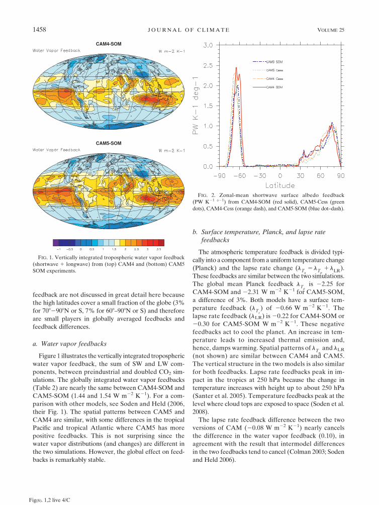
Figure 1 illustrates the vertically integrated tropospheric
water vapor feedback, the sum of SW and LW com-
ponents, between preindustrial and doubled CO2 sim-
ulations. The globally integrated water vapor feedbacks
(Table 2) are nearly the same between CAM4-SOM and
CAM5-SOM (1.44 and 1.54 W m22 K21). For a com-
parison with other models, see Soden and Held (2006,
their Fig. 1). The spatial patterns between CAM5 and
CAM4 are similar, with some differences in the tropical
Pacific and tropical Atlantic where CAM5 has more
positive feedbacks. This is not surprising since the
water vapor distributions (and changes) are different in
the two simulations. However, the global effect on feed-
backs is remarkably stable.
b. Surface temperature, Planck, and lapse ratefeedbacks
The atmospheric temperature feedback is divided typi-
cally into a component from a uniform temperature change
(Planck) and the lapse rate change (lTa5 lTp
1 lLR).
These feedbacks are similar between the two simulations.
The global mean Planck feedback lTp
is 22.25 for
CAM4-SOM and 22.31 W m22 K21 for CAM5-SOM,
a difference of 3%. Both models have a surface tem-
perature feedback (lTs
) of 20.66 W m22 K21. The
lapse rate feedback (lLR) is 20.22 for CAM4-SOM or
20.30 for CAM5-SOM W m22 K21. These negative
feedbacks act to cool the planet. An increase in tem-
perature leads to increased thermal emission and,
hence, damps warming. Spatial patterns of lTp
and lLR
(not shown) are similar between CAM4 and CAM5.
The vertical structure in the two models is also similar
for both feedbacks. Lapse rate feedbacks peak in im-
pact in the tropics at 250 hPa because the change in
temperature increases with height up to about 250 hPa
(Santer et al. 2005). Temperature feedbacks peak at the
level where cloud tops are exposed to space (Soden et al.
2008).
The lapse rate feedback difference between the two
versions of CAM (20.08 W m22 K21) nearly cancels
the difference in the water vapor feedback (0.10), in
agreement with the result that intermodel differences
in the two feedbacks tend to cancel (Colman 2003; Soden
and Held 2006).
FIG. 1. Vertically integrated tropospheric water vapor feedback
(shortwave 1 longwave) from (top) CAM4 and (bottom) CAM5
SOM experiments.
FIG. 2. Zonal-mean shortwave surface albedo feedback
(PW K21 821) from CAM4-SOM (red solid), CAM5-Cess (green
dots), CAM4-Cess (orange dash), and CAM5-SOM (blue dot–dash).
Fig(s). 1,2 live 4/C
1458 J O U R N A L O F C L I M A T E VOLUME 25
c. Surface albedo feedbacks
Surface albedo feedbacks (la) are similar between
CAM4 and CAM5 with a difference of 0.03 W m22 K21,
or 9% (Table 2). The zonal mean surface albedo feed-
backs for the CAM4 and CAM5 SOM runs are illus-
trated in Fig. 2 (in PW deg21 K21). The feedbacks are
sharply peaked in the Southern Hemisphere, corre-
sponding to the region of sea ice loss. In the Northern
Hemisphere, the region is much broader as both sea ice
and land ice and snow contribute. CAM4 has more
positive feedbacks in the Southern Hemisphere. In
both hemispheres, the regions making large contributions
to the albedo feedback in CAM5 tend to be shifted
slightly to higher latitudes due to differences in the
mean sea ice edge.
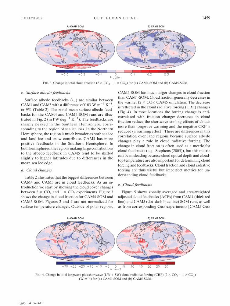
d. Cloud changes
Table 2 illustrates that the biggest differences between
CAM4 and CAM5 are in cloud feedbacks. As an in-
troduction we start by showing the cloud cover changes
between 2 3 CO2 and 1 3 CO2 experiments. Figure 3
shows the change in cloud fraction for CAM4-SOM and
CAM5-SOM. Figures 3 and 4 are not normalized for
surface temperature changes. Outside of polar regions,
CAM5-SOM has much larger changes in cloud fraction
than CAM4-SOM. Cloud fraction generally decreases in
the warmer (2 3 CO2) CAM5 simulation. The decrease
is reflected in the cloud radiative forcing (CRF) changes
(Fig. 4). In most locations the forcing change is anti-
correlated with fraction change: decreases in cloud
fraction reduce the shortwave cooling effects of clouds
more than longwave warming and the negative CRF is
reduced (a warming effect). There are differences in this
correlation over land regions because surface albedo
changes play a role in cloud radiative forcing. The
change in cloud fraction is often used as a metric for
cloud feedbacks (e.g., Stephens (2005)), but this metric
can be misleading because cloud optical depth and cloud-
top temperature are also important for determining cloud
forcing and feedbacks. Cloud fraction and cloud radiative
forcing are thus useful but imperfect metrics for un-
derstanding cloud feedbacks.
e. Cloud feedbacks
Figure 5 shows zonally averaged and area-weighted
adjusted cloud feedbacks (ACFs) from CAM4 (thick red
line) and CAM5 (dot–dash blue line) SOM runs, as well
as from corresponding Cess experiments [CAM5 Cess
FIG. 3. Change in total cloud fraction (2 3 CO2 2 1 3 CO2) for (a) CAM4-SOM and (b) CAM5-SOM.
FIG. 4. Change in total longwave plus shortwave (LW 1 SW) cloud radiative forcing (CRF) (2 3 CO2 2 1 3 CO2)
(W m22) for (a) CAM4-SOM and (b) CAM5-SOM.
Fig(s). 3,4 live 4/C
1 MARCH 2012 G E T T E L M A N E T A L . 1459
(green), CAM4 Cess (orange)]. For clarity, we omit high
latitudes poleward of 608 since the area falls off rapidly
and the adjustment depends strongly on surface prop-
erties (sea ice and snow). These regions have specified
sea ice in Cess runs and so are not fully treated by this
method.
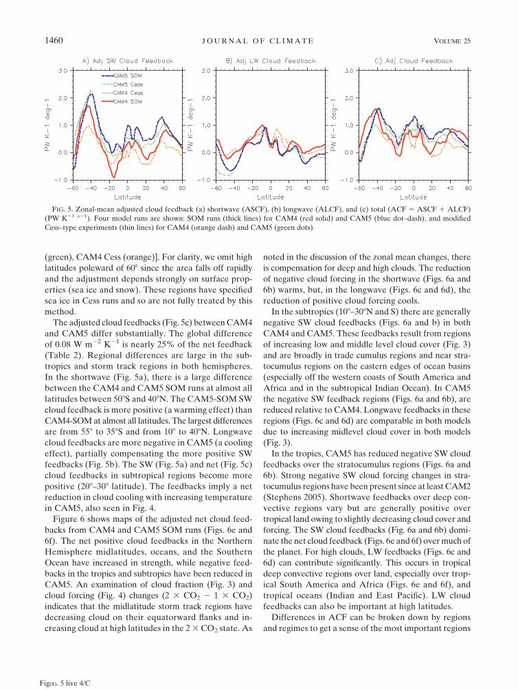
The adjusted cloud feedbacks (Fig. 5c) between CAM4
and CAM5 differ substantially. The global difference
of 0.08 W m22 K21 is nearly 25% of the net feedback
(Table 2). Regional differences are large in the sub-
tropics and storm track regions in both hemispheres.
In the shortwave (Fig. 5a), there is a large difference
between the CAM4 and CAM5 SOM runs at almost all
latitudes between 508S and 408N. The CAM5-SOM SW
cloud feedback is more positive (a warming effect) than
CAM4-SOM at almost all latitudes. The largest differences
are from 558 to 358S and from 108 to 408N. Longwave
cloud feedbacks are more negative in CAM5 (a cooling
effect), partially compensating the more positive SW
feedbacks (Fig. 5b). The SW (Fig. 5a) and net (Fig. 5c)
cloud feedbacks in subtropical regions become more
positive (208–308 latitude). The feedbacks imply a net
reduction in cloud cooling with increasing temperature
in CAM5, also seen in Fig. 4.
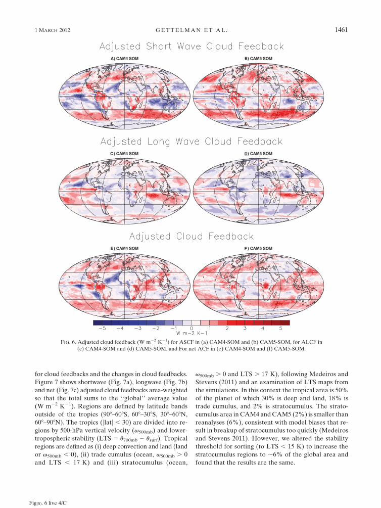
Figure 6 shows maps of the adjusted net cloud feed-
backs from CAM4 and CAM5 SOM runs (Figs. 6e and
6f). The net positive cloud feedbacks in the Northern
Hemisphere midlatitudes, oceans, and the Southern
Ocean have increased in strength, while negative feed-
backs in the tropics and subtropics have been reduced in
CAM5. An examination of cloud fraction (Fig. 3) and
cloud forcing (Fig. 4) changes (2 3 CO2 2 1 3 CO2)
indicates that the midlatitude storm track regions have
decreasing cloud on their equatorward flanks and in-
creasing cloud at high latitudes in the 2 3 CO2 state. As
noted in the discussion of the zonal mean changes, there
is compensation for deep and high clouds. The reduction
of negative cloud forcing in the shortwave (Figs. 6a and
6b) warms, but, in the longwave (Figs. 6c and 6d), the
reduction of positive cloud forcing cools.
In the subtropics (108–308N and S) there are generally
negative SW cloud feedbacks (Figs. 6a and b) in both
CAM4 and CAM5. These feedbacks result from regions
of increasing low and middle level cloud cover (Fig. 3)
and are broadly in trade cumulus regions and near stra-
tocumulus regions on the eastern edges of ocean basins
(especially off the western coasts of South America and
Africa and in the subtropical Indian Ocean). In CAM5
the negative SW feedback regions (Figs. 6a and 6b), are
reduced relative to CAM4. Longwave feedbacks in these
regions (Figs. 6c and 6d) are comparable in both models
due to increasing midlevel cloud cover in both models
(Fig. 3).
In the tropics, CAM5 has reduced negative SW cloud
feedbacks over the stratocumulus regions (Figs. 6a and
6b). Strong negative SW cloud forcing changes in stra-
tocumulus regions have been present since at least CAM2
(Stephens 2005). Shortwave feedbacks over deep con-
vective regions vary but are generally positive over
tropical land owing to slightly decreasing cloud cover and
forcing. The SW cloud feedbacks (Fig. 6a and 6b) domi-
nate the net cloud feedback (Figs. 6e and 6f) over much of
the planet. For high clouds, LW feedbacks (Figs. 6c and
6d) can contribute significantly. This occurs in tropical
deep convective regions over land, especially over trop-
ical South America and Africa (Figs. 6e and 6f), and
tropical oceans (Indian and East Pacific). LW cloud
feedbacks can also be important at high latitudes.
Differences in ACF can be broken down by regions
and regimes to get a sense of the most important regions
FIG. 5. Zonal-mean adjusted cloud feedback (a) shortwave (ASCF), (b) longwave (ALCF), and (c) total (ACF 5 ASCF 1 ALCF)
(PW K21 821). Four model runs are shown: SOM runs (thick lines) for CAM4 (red solid) and CAM5 (blue dot–dash), and modified
Cess–type experiments (thin lines) for CAM4 (orange dash) and CAM5 (green dots).
Fig(s). 5 live 4/C
1460 J O U R N A L O F C L I M A T E VOLUME 25
for cloud feedbacks and the changes in cloud feedbacks.
Figure 7 shows shortwave (Fig. 7a), longwave (Fig. 7b)
and net (Fig. 7c) adjusted cloud feedbacks area-weighted
so that the total sums to the ‘‘global’’ average value
(W m22 K21). Regions are defined by latitude bands
outside of the tropics (908–608S, 608–308S, 308–608N,
608–908N). The tropics (jlatj , 30) are divided into re-
gions by 500-hPa vertical velocity (v500mb) and lower-
tropospheric stability (LTS 5 u700mb 2 usurf). Tropical
regions are defined as (i) deep convection and land (land
or v500mb , 0), (ii) trade cumulus (ocean, v500mb . 0
and LTS , 17 K) and (iii) stratocumulus (ocean,
v500mb . 0 and LTS . 17 K), following Medeiros and
Stevens (2011) and an examination of LTS maps from
the simulations. In this context the tropical area is 50%
of the planet of which 30% is deep and land, 18% is
trade cumulus, and 2% is stratocumulus. The strato-
cumulus area in CAM4 and CAM5 (2%) is smaller than
reanalyses (6%), consistent with model biases that re-
sult in breakup of stratocumulus too quickly (Medeiros
and Stevens 2011). However, we altered the stability
threshold for sorting (to LTS , 15 K) to increase the
stratocumulus regions to ;6% of the global area and
found that the results are the same.
FIG. 6. Adjusted cloud feedback (W m22 K21) for ASCF in (a) CAM4-SOM and (b) CAM5-SOM, for ALCF in
(c) CAM4-SOM and (d) CAM5-SOM, and For net ACF in (e) CAM4-SOM and (f) CAM5-SOM.
Fig(s). 6 live 4/C
1 MARCH 2012 G E T T E L M A N E T A L . 1461
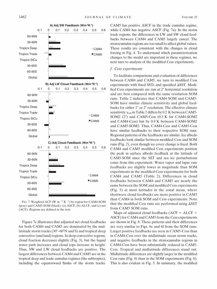
Figure 7c illustrates that adjusted net cloud feedbacks
for both CAM4 and CAM5 are dominated by the mid-
latitude storm tracks (308–608N and S) and tropical deep
convective (and land) regions. In deep convective regions,
cloud fraction decreases slightly (Fig. 3), but the liquid
water path increases and cloud tops increase in height.
Thus, SW and LW cloud feedbacks are positive. The
largest differences between CAM4 and CAM5 are in the
tropical deep and trade cumulus regimes (the subtropics),
including the equatorward flanks of the storm tracks.
CAM5 has positive ASCF in the trade cumulus regime,
while CAM4 has negative ASCF (Fig. 7a). In the storm
track regions, the differences in LW and SW cloud feed-
backs between CAM4 and CAM5 largely cancel. The
stratocumulus regions are too small to affect global values.
These results are consistent with the changes in cloud
forcing in Fig. 4. To understand which parameterization
changes to the model are important in these regimes, we
next turn to analysis of the modified Cess experiments.
f. Cess experiments
To facilitate comparisons and evaluation of differences
between CAM4 and CAM5, we turn to modified Cess
experiments with fixed SSTs and specified DSST. Modi-
fied Cess experiments are run at 28 horizontal resolution
and are best compared with the same resolution SOM
runs. Table 2 indicates that CAM4-SOM and CAM5-
SOM have similar climate sensitivity and global feed-
backs for either 18 or 28 resolution. The effective climate
sensitivity geff in Table 2 differs by 0.2 K between CAM5-
SOM2 (28) and CAM5-Cess (0.3 K for CAM4-SOM2
and CAM4-Cess) but by 0.9 K between CAM4-SOM2
and CAM5-SOM2. Thus, CAM4-Cess and CAM5-Cess
have similar feedbacks to their respective SOM runs.
Regional patterns of the feedbacks are similar. Ice albedo
feedbacks look similar between modified Cess and SOM
runs (Fig. 2), even though ice cover change is fixed. Both
CAM4 and CAM5 modified Cess experiments position
the peak in surface albedo feedback at the latitude of
CAM5-SOM since the SST and sea ice perturbations
come from this experiment. Water vapor and lapse rate
feedbacks are slightly lower in magnitude than SOM
experiments in the modified Cess experiments for both
CAM4 and CAM5 (Table 2). Differences in cloud
feedbacks between CAM4 and CAM5 are nearly the
same between the SOM and modified Cess experiments
(Fig. 5) at most latitudes in the zonal mean, where
shortwave cloud feedbacks are more positive in CAM5
than CAM4 in both SOM and Cess experiments. Note
that the modified Cess runs are performed using DSST
from CAM5 SOM runs.
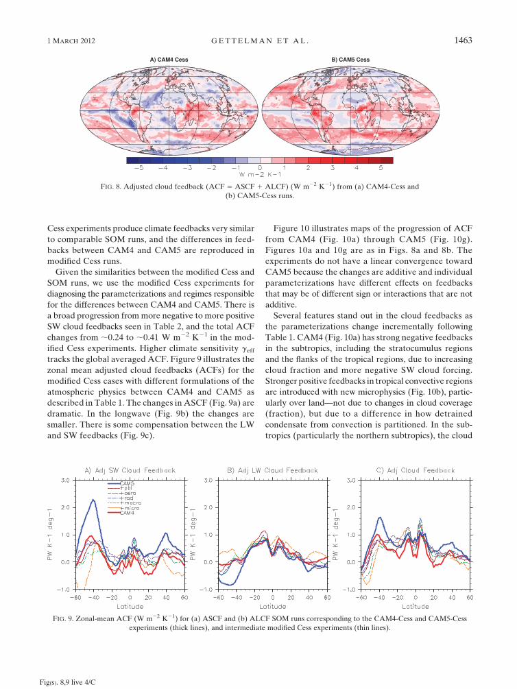
Maps of adjusted cloud feedbacks (ACF 5 ALCF 1
ASCF) for CAM4 and CAM5 from the Cess experiments
are shown in Fig. 8. These patterns and their differences
are very similar to Figs. 6e and 6f from the SOM runs.
Larger positive feedbacks are seen in CAM5-Cess than
in CAM4-Cess over the midlatitude ocean storm tracks,
and negative feedbacks in the stratocumulus regions in
CAM4-Cess have been substantially reduced in CAM5-
Cess. Tropical and midlatitude differences stand out.
Midlatitude differences are slightly larger in the modified
Cess runs (Fig. 8) than in the SOM experiments (Fig. 6).
This is also evident in Fig. 5. In summary, the modified
FIG. 7. Weighted ACF (W m22 K21) by region for CAM4-SOM
(gray) and CAM5-SOM (black): (a) ASCF, (b) ALCF, and (c) net
(ACF). Regions are defined in the text.
1462 J O U R N A L O F C L I M A T E VOLUME 25
Cess experiments produce climate feedbacks very similar
to comparable SOM runs, and the differences in feed-
backs between CAM4 and CAM5 are reproduced in
modified Cess runs.
Given the similarities between the modified Cess and
SOM runs, we use the modified Cess experiments for
diagnosing the parameterizations and regimes responsible
for the differences between CAM4 and CAM5. There is
a broad progression from more negative to more positive
SW cloud feedbacks seen in Table 2, and the total ACF
changes from ;0.24 to ;0.41 W m22 K21 in the mod-
ified Cess experiments. Higher climate sensitivity geff
tracks the global averaged ACF. Figure 9 illustrates the
zonal mean adjusted cloud feedbacks (ACFs) for the
modified Cess cases with different formulations of the
atmospheric physics between CAM4 and CAM5 as
described in Table 1. The changes in ASCF (Fig. 9a) are
dramatic. In the longwave (Fig. 9b) the changes are
smaller. There is some compensation between the LW
and SW feedbacks (Fig. 9c).
Figure 10 illustrates maps of the progression of ACF
from CAM4 (Fig. 10a) through CAM5 (Fig. 10g).
Figures 10a and 10g are as in Figs. 8a and 8b. The
experiments do not have a linear convergence toward
CAM5 because the changes are additive and individual
parameterizations have different effects on feedbacks
that may be of different sign or interactions that are not
additive.
Several features stand out in the cloud feedbacks as
the parameterizations change incrementally following
Table 1. CAM4 (Fig. 10a) has strong negative feedbacks
in the subtropics, including the stratocumulus regions
and the flanks of the tropical regions, due to increasing
cloud fraction and more negative SW cloud forcing.
Stronger positive feedbacks in tropical convective regions
are introduced with new microphysics (Fig. 10b), partic-
ularly over land—not due to changes in cloud coverage
(fraction), but due to a difference in how detrained
condensate from convection is partitioned. In the sub-
tropics (particularly the northern subtropics), the cloud
FIG. 8. Adjusted cloud feedback (ACF 5 ASCF 1 ALCF) (W m22 K21) from (a) CAM4-Cess and
(b) CAM5-Cess runs.
FIG. 9. Zonal-mean ACF (W m22 K21) for (a) ASCF and (b) ALCF SOM runs corresponding to the CAM4-Cess and CAM5-Cess
experiments (thick lines), and intermediate modified Cess experiments (thin lines).
Fig(s). 8,9 live 4/C
1 MARCH 2012 G E T T E L M A N E T A L . 1463
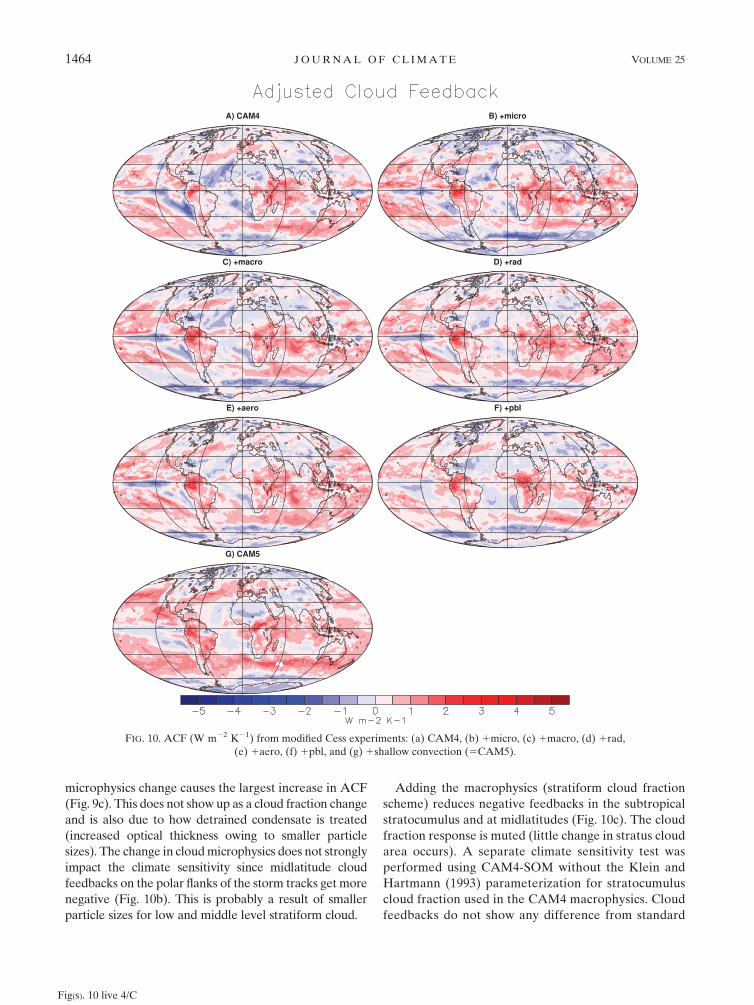
microphysics change causes the largest increase in ACF
(Fig. 9c). This does not show up as a cloud fraction change
and is also due to how detrained condensate is treated
(increased optical thickness owing to smaller particle
sizes). The change in cloud microphysics does not strongly
impact the climate sensitivity since midlatitude cloud
feedbacks on the polar flanks of the storm tracks get more
negative (Fig. 10b). This is probably a result of smaller
particle sizes for low and middle level stratiform cloud.
Adding the macrophysics (stratiform cloud fraction
scheme) reduces negative feedbacks in the subtropical
stratocumulus and at midlatitudes (Fig. 10c). The cloud
fraction response is muted (little change in stratus cloud
area occurs). A separate climate sensitivity test was
performed using CAM4-SOM without the Klein and
Hartmann (1993) parameterization for stratocumulus
cloud fraction used in the CAM4 macrophysics. Cloud
feedbacks do not show any difference from standard
FIG. 10. ACF (W m22 K21) from modified Cess experiments: (a) CAM4, (b) 1micro, (c) 1macro, (d) 1rad,
(e) 1aero, (f) 1pbl, and (g) 1shallow convection (5CAM5).
Fig(s). 10 live 4/C
1464 J O U R N A L O F C L I M A T E VOLUME 25
CAM4-SOM, consistent with the small stratocumulus
area (Fig. 7).
Introducing the radiation code and cloud optics makes
tropical cloud feedbacks (Fig. 10d) more positive in the
Indian Ocean. This appears to be due to a LW cloud
forcing change resulting from changes in the ice cloud
optics. The global climate sensitivity increases sub-
stantially (Table 2) because of a jump in the shortwave
(and total) cloud feedbacks (Table 2). The sensitivity
also increases because offline calculations (Kay et al.
2011, manuscript submitted to J. Climate) show an in-
crease in the CO2 radiative forcing GCO 2
of about 10%
(from 3.5 to 3.8 W m22 for doubling CO2 from 280 to 560
ppmv) with the Rapid Radiative Transfer Model for
GCMs radiation code.
The introduction of the aerosol scheme and new aerosol
optics (that alter the direct radiative effect of aerosols)
does not have a strong impact on cloud feedback (Figs.
10e) or overall climate sensitivity (Table 2). This assumes
constant aerosol emissions for present-day conditions.
The new boundary layer scheme increases negative
feedbacks in the subtropics and tropics (Figs. 10f and
9c). This occurs in the subtropics, mostly in the SW (Fig.
9a), because of larger increases in low-cloud fraction in
the subtropics with the addition of the new PBL scheme.
This increase enhances negative SW cloud feedbacks
and corresponds to the only large decrease in the climate
sensitivity in the progression between CAM4 and
CAM5 (Table 2).
The introduction of the shallow cumulus scheme is the
last piece that makes up CAM5, and its introduction has
the largest impact on ACF (difference between Figs. 10f
and 10g). The effects are largest in the oceanic mid-
latitude storm tracks and extend to the edge of the sub-
tropics. Effects are due to cloud fraction changes
(reductions) extending farther equatorward in these
simulations. Differences are also clear in the zonal mean
(Fig. 9). The reductions in cloud cause increases in ASCF
in the storm tracks (Fig. 9a) and are consistent with
a larger reduction in the shallow convection mass flux for
the 2 3 CO2 case in CAM5 over CAM4.
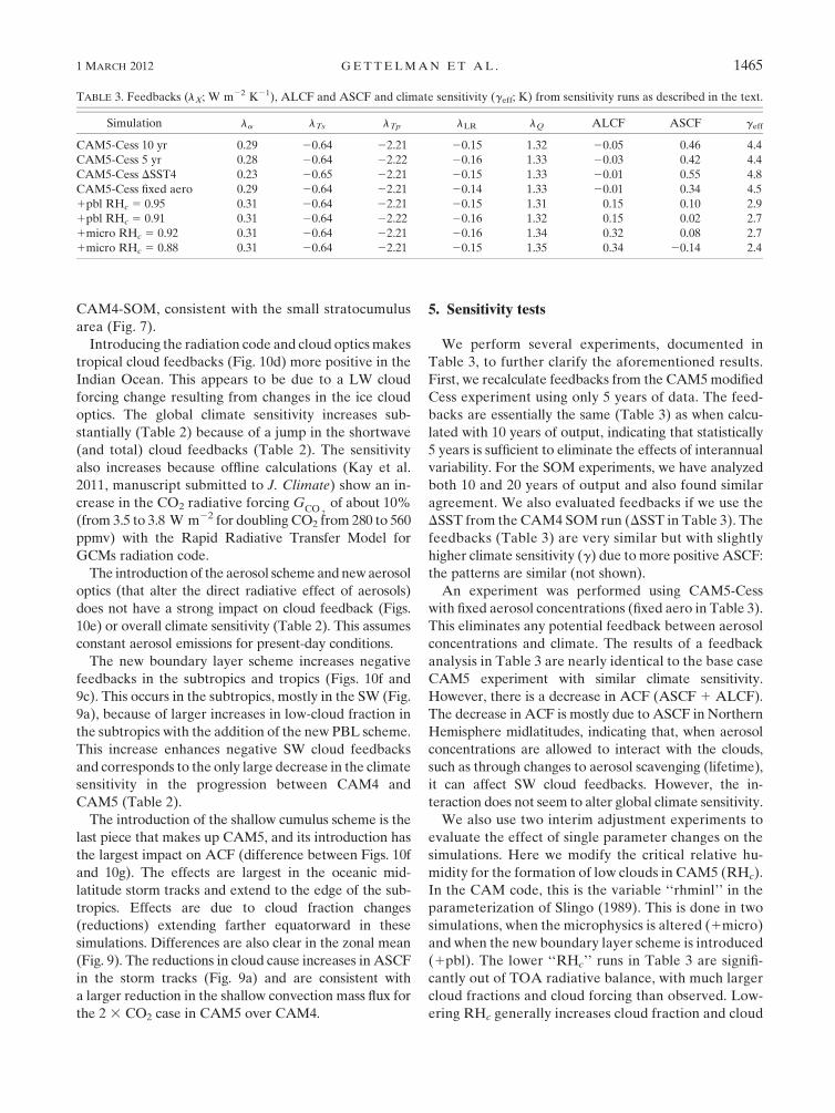
5. Sensitivity tests
We perform several experiments, documented in
Table 3, to further clarify the aforementioned results.
First, we recalculate feedbacks from the CAM5 modified
Cess experiment using only 5 years of data. The feed-
backs are essentially the same (Table 3) as when calcu-
lated with 10 years of output, indicating that statistically
5 years is sufficient to eliminate the effects of interannual
variability. For the SOM experiments, we have analyzed
both 10 and 20 years of output and also found similar
agreement. We also evaluated feedbacks if we use the
DSST from the CAM4 SOM run (DSST in Table 3). The
feedbacks (Table 3) are very similar but with slightly
higher climate sensitivity (g) due to more positive ASCF:
the patterns are similar (not shown).
An experiment was performed using CAM5-Cess
with fixed aerosol concentrations (fixed aero in Table 3).
This eliminates any potential feedback between aerosol
concentrations and climate. The results of a feedback
analysis in Table 3 are nearly identical to the base case
CAM5 experiment with similar climate sensitivity.
However, there is a decrease in ACF (ASCF 1 ALCF).
The decrease in ACF is mostly due to ASCF in Northern
Hemisphere midlatitudes, indicating that, when aerosol
concentrations are allowed to interact with the clouds,
such as through changes to aerosol scavenging (lifetime),
it can affect SW cloud feedbacks. However, the in-
teraction does not seem to alter global climate sensitivity.
We also use two interim adjustment experiments to
evaluate the effect of single parameter changes on the
simulations. Here we modify the critical relative hu-
midity for the formation of low clouds in CAM5 (RHc).
In the CAM code, this is the variable ‘‘rhminl’’ in the
parameterization of Slingo (1989). This is done in two
simulations, when the microphysics is altered (1micro)
and when the new boundary layer scheme is introduced
(1pbl). The lower ‘‘RHc’’ runs in Table 3 are signifi-
cantly out of TOA radiative balance, with much larger
cloud fractions and cloud forcing than observed. Low-
ering RHc generally increases cloud fraction and cloud
TABLE 3. Feedbacks (lX; W m22 K21), ALCF and ASCF and climate sensitivity (geff; K) from sensitivity runs as described in the text.
Simulation la lTs lTp lLR lQ ALCF ASCF geff
CAM5-Cess 10 yr 0.29 20.64 22.21 20.15 1.32 20.05 0.46 4.4
CAM5-Cess 5 yr 0.28 20.64 22.22 20.16 1.33 20.03 0.42 4.4
CAM5-Cess DSST4 0.23 20.65 22.21 20.15 1.33 20.01 0.55 4.8
CAM5-Cess fixed aero 0.29 20.64 22.21 20.14 1.33 20.01 0.34 4.5
1pbl RHc 5 0.95 0.31 20.64 22.21 20.15 1.31 0.15 0.10 2.9
1pbl RHc 5 0.91 0.31 20.64 22.22 20.16 1.32 0.15 0.02 2.7
1micro RHc 5 0.92 0.31 20.64 22.21 20.16 1.34 0.32 0.08 2.7
1micro RHc 5 0.88 0.31 20.64 22.21 20.15 1.35 0.34 20.14 2.4
1 MARCH 2012 G E T T E L M A N E T A L . 1465
forcing. The runs with larger cloud fraction (lower
RHc) and larger cloud forcing have reduced ASCF and
reduced climate sensitivity. In both of these cases,
thicker low clouds (higher gross SW cloud forcing) tend
to lower climate sensitivity (geff) in these CAM5-Cess
simulations.
In summary, the feedback calculations are robust with
respect to the time period and input SST used. We also
note from Table 2 that feedbacks are not affected by
horizontal resolution in the CAM4 and CAM5 SOM
runs. Aerosols appear to have a small impact on SW
cloud feedbacks, but not climate sensitivity. The di-
agnosis of feedbacks also appears fairly stable to some
of the more commonly used gross cloud adjustment
parameters in climate models, with the caveat that the
changes to clouds may matter for climate sensitivity,
and higher mean cloud forcing results in decreased
ASCF and lower climate sensitivity.
6. Discussion
A series of experiments has been conducted to try to
understand what processes and regions are responsible
for the change in cloud feedbacks between two versions
of CAM. Model configurations with fixed ocean tem-
perature perturbations derived from coupled slab ocean
model runs are able to reproduce feedbacks in the
SOM experiments, allowing us to use the less compu-
tationally intensive modified Cess experiments (fol-
lowing Cess et al. 1990). Modified Cess experiments can
reproduce key climate feedbacks seen in SOM runs, in
contrast to traditional Cess experiments (Senior and
Mitchell 1993; Ringer et al. 2006). Furthermore, global
climate sensitivity and climate feedbacks do not appear
sensitive to model horizontal resolution (18 or 28) in
either CAM4 or CAM5.
CAM5 has a higher climate sensitivity than CAM4.
Water vapor, temperature, and lapse rate feedbacks as
well as surface albedo feedbacks are basically the same
between the two models. The difference in sensitivity
is mostly due to (i) changes in cloud feedbacks and
(ii) a difference in GCO2
between CAM4 and CAM5.
The GCO2
is a function of the model state (e.g., the
temperature, cloud, and water vapor distribution) and
the radiative transfer code. Calculations (see Kay et al.
2011, manuscript submitted to J. Climate) indicate
GCO25 3:5 W m22 for CAM4 and 3.8 W m22 for
CAM5. The result is consistent with calculations by
Iacono et al. (2008), who indicate that the difference is
due to the radiative transfer code itself (not model
state). Assuming a constant total feedback strength (l)
of 21 W m22 K21 in Eq. (2), this yields a difference in
climate sensitivity (DTas) of 0.3 K, or about 40% of the
0.8-K difference in sensitivity between CAM4-SOM
and CAM5-SOM (Table 2).
There is uncertainty that comes into the nonlinear
term (NT) in Eq. (3): NT can be calculated by estimating
the total feedback (l) for CAM4 and CAM5 as leff [Eq.
(5)] with GCO2differing for CAM4 and CAM5, and DTas
and H as the difference in temperature and TOA bal-
ance, respectively, between the 2 3 CO2 and 1 3 CO2
SOM runs. This allows a closed sum of feedbacks. For
CAM5-SOM H 5 20.005 W m22, so leff 5 (3.8 2
0.005)/4.0 5 20.95 W m22 K21. For CAM4-SOM H 5
20.075, so leff 5 (3.5 2 0.075)/3.2 5 21.07 W m22 K21.
The sum of the feedbacks from Table 2 does not equal
this (20.92 for CAM4-SOM, 20.91 for CAM5-SOM)
This means that the nonlinear term NT 5 10.04 for
CAM5-SOM and 10.15 for CAM4-SOM. This is a
measure of the uncertainty and, for CAM4, is larger
than the 10% estimate of Shell et al. (2008). The clouds
differ by 0.08 W m22 K21 (with CAM5 higher). This is
offset by differences of 20.03 and 20.06 in albedo and
Planck feedbacks, representing small fractional changes
in these feedbacks (9% and 3%, respectively). There is
10%–20% uncertainty in the feedbacks due to NT.
After factoring in the change in radiative forcing,
cloud feedbacks account for much of the remaining
difference between the climate sensitivity in CAM4 and
CAM5 and the largest percent difference in feedbacks
(25%). The 0.08 W m22 K21 difference in net cloud
feedback between CAM4-SOM and CAM5-SOM masks
larger changes in SW (10.29) and LW (20.21) compo-
nents, indicating a very different cloud response in CAM5
from CAM4. Using perturbations to Eq. (3), the net
cloud feedback difference of 0.08 W m22 K21 between
CAM5-SOM and CAM4-SOM accounts for another
;0.26–0.37 K (30%–50%) of the difference in climate
sensitivity, depending on whether CAM4 or CAM5
values of GCO2and leff are used in Eq. (3).
The changes in cloud feedbacks are spatially coherent.
Negative cloud feedbacks in the tropics decrease in the
CAM5 experiments, while positive cloud feedbacks in-
crease over the subtropics and in the storm track re-
gions. Tropical changes are due to reductions in negative
feedbacks with a new cloud microphysics and macro-
physics scheme. The microphysics affects convective
detrainment, and the macrophysics mutes cloud fraction
changes in trade cumulus regimes in the subtropics. The
new PBL scheme tends to increase negative cloud
feedbacks through increased subtropical cloud fraction
and reduce climate sensitivity, counteracting the changes
from the microphysics. In the subtropics and mid-
latitudes, positive increases of cloud forcing in the
equatorward portion of the stormtrack regions (due to
larger decreases in cloud fraction) occur with the
1466 J O U R N A L O F C L I M A T E VOLUME 25
introduction of the new shallow convection (cumulus)
scheme, enhancing climate sensitivity. The new shallow
cumulus scheme alters the interaction between stratus
and shallow cumulus clouds and has a major effect on
the flanks of the storm tracks. Larger decreases in shallow
convective mass flux are occurring in CAM5 for 2 3 CO2
conditions, decreasing cloud in broad regions as the storm
tracks shift poleward. The poleward shift in the 2 3 CO2
simulations is consistent with observations (Seidel et al.
2008) and other model simulations (Son et al. 2009) and is
about the same in both CAM4 and CAM5, but the effect
on clouds is larger in CAM5.
Notably, these changes are not strongly due to the
subtropical marine stratocumulus regions. When cloud
feedbacks are weighted by area, these regions are less
important as they represent only 2%–6% of the area of
the planet. These small regions may be more important
in a fully coupled system with ocean dynamics, yet given
their limited area the stratocumulus region impact on
global feedback strength is inherently limited. From
these experiments it appears that cumulus clouds in the
subtropics and storm track regions exert the strongest
lever on global climate sensitivity. This conclusion is
supported by previous work. Bony et al. (2004) noted
that it was regions of moderate subsidence (trade cu-
mulus) that have the highest frequency and largest effect
on tropical averaged cloud forcing, and Medeiros et al.
(2008) found that the shallow cumulus regime was
most important for cloud forcing and feedback. While
Williams and Webb (2009) stress the importance of low
clouds for cloud feedback, half of their global signal is
from outside of the tropical regions. The results are
consistent with recent work by Trenberth and Fasullo
(2010), who found a relationship between cloudiness in
the SH storm track (a canonical bias in models) and
model climate sensitivity.
In the CAM5 simulations, as the planet warms, low
clouds become less extensive and the storm tracks move
poleward. The change in cloudiness and cloud forcing is
most strongly impacted by shallow convective clouds
and is strongly correlated with decreases in shallow
convective mass flux. One likely mechanism is that the
reduced mass flux alters detrainment into stratiform
clouds, reducing the liquid water path and allowing for
a larger change (reduction) in the (negative) cloud
forcing.
Perturbation tests reveal two additional important
features of the simulations. First, tests at two different
points in the model development process indicated that
climate sensitivity does appear to be coherently de-
creased by ;10% as cloud forcing increases. In these
experiments, a climate state with more cloud radia-
tive forcing (thicker clouds with more water substance
and/or larger horizontal extent) implies a smaller per-
centage change in cloud forcing response and lower
climate sensitivity. This is likely due to the nonlinear
effects of radiative transfer: bands where cloud is
important in the LW and SW saturate, and further
changes to cloud forcing are reduced with increased
cloudiness. Expanding on this hypothesis, high water
content clouds can especially dampen warming over an
ice-covered ocean. Kay et al. (2011, manuscript sub-
mitted to J. Climate) find that the high water content
Arctic clouds in CAM4 dampen greenhouse warming
both with negative Arctic shortwave cloud feedbacks
and by masking the surface, reducing positive surface
albedo feedbacks.
Second, fixing aerosol concentrations in CAM5-Cess
decreased SW cloud feedbacks. The decreased feedback
implies that interactive prognostic aerosols play a role in
understanding cloud feedback responses; however, the
effects on climate sensitivity are not conclusive, and the
results are not seen with the introduction of the new
aerosol scheme (Table 2). This may indicate a complex
interaction of several different parameterizations be-
tween clouds and aerosols.
7. Conclusions
This work highlights the evolution of climate sensi-
tivity in CAM from version 4 (3.2 K) to version 5
(4.0 K). It also highlights the utility of modified ‘‘Cess’’
experiments to diagnose feedbacks. The increase in
sensitivity is due to changes in CO2 radiative forcing
(40%) and most of the remainder is due to changes in
cloud feedbacks. Changes in cloud feedbacks primarily
occur in the tropics and midlatitudes. Changes to water
vapor, lapse rate, and albedo feedbacks are not strong
contributors to changes in global climate sensitivity
between CAM4 and CAM5.
Several parameterizations contribute to cloud changes
in the tropics and a reduction of negative feedbacks in the
subtropics. The shallow cumulus scheme is important for
enhancing positive cloud feedbacks in the subtropics and
midlatitudes. The equatorward branches of the storm
tracks and deep convective regions contribute most to the
global change in cloud feedbacks. Stratocumulus regions
in the tropics and subtropics do not strongly contribute
to the change in cloud feedbacks or climate sensitivity.
Further work will be necessary to understand the exact
mechanisms that alter the climate sensitivity.
These results hint at relationships between clouds and
climate sensitivity. CAM4 and CAM5 span a wide range
of structural parameterization differences. In perturba-
tion experiments, climate states with higher cloud forc-
ing are less sensitive than those with thinner clouds. This
1 MARCH 2012 G E T T E L M A N E T A L . 1467
may be location and regime specific. Further work is
necessary to (i) test these conclusions across a broader
spectrum of models and (ii) compare model states with
observations of key cloud parameters to attempt to better
constrain climate sensitivity. Current observational con-
straints imply cloud feedbacks similar to what is de-
scribed here (Dessler 2010), but do not have sufficient
precision to constrain climate sensitivity. Given the cur-
rent uncertainty in global estimates of important cloud
properties, it is critical to get better observations (both
mean state and variability) in different regions (such as
the subtropics and the Southern Ocean).
Acknowledgments. KMS was supported by the
National Science Foundation Grant ATM-0904092.
Thanks are given to C. Hannay for assistance with
runs and J. T. Kiehl for key insights. We also thank B.
Medieros, K. E. Trenberth, and J. T. Fasullo for discussions.
REFERENCES
Bitz, C., K. Shell, P. Gent, D. Bailey, G. Danabasoglu, K. Armour,
M. Holland, and J. Kiehl, 2012: Climate sensitivity of the
Community Climate System Model version 4. J. Climate, in
press.
Bony, S., and J.-L. Dufresne, 2005: Marine boundary layer clouds
at the heart of tropical cloud feedback uncertainties in cli-
mate models. Geophys. Res. Lett., 32, L20806, doi:10.1029/
2005GL023851.
——, ——, H. Le Treut, J.-J. Morcrette, and C. Senior, 2004: On
dynamic and thermodynamic components of cloud changes.
Climate Dyn., 22, 71–86, doi:10.1007/s00382-003-0369-6.
——, and Coauthors, 2006: How well do we understand and
evaluate climate change feedback processes? J. Climate, 19,
3445–3482.
Bretherton, C. S., and S. Park, 2009: A new moist turbulence pa-
rameterization in the Community Atmosphere Model. J. Cli-
mate, 22, 3422–3448.
Cess, R. D., and Coauthors, 1990: Intercomparison and interpretation
of climate feedback processes in 19 atmospheric general circu-
lation models. J. Geophys. Res., 95, 16 601–16 615.
——, and Coauthors, 1996: Cloud feedback in atmospheric general
circulation models: An update. J. Geophys. Res., 101 (D8),
12 791–12 794.
Collins, W. D., and Coauthors, 2004: Description of the NCAR
Community Atmosphere Model (CAM 3.0). NCAR Tech.
Note NCAR/TN-4641STR, 226 pp.
——, and Coauthors, 2006: The formulation and atmospheric
simulation of the Community Atmosphere Model Version 3
(CAM3). J. Climate, 19, 2122–2161.
Colman, R., 2003: A comparison of climate feedbacks in general
circulation models. Climate Dyn., 20, 865–873.
Dessler, A. E., 2010: A determination of the cloud feedback from
climate variations over the past decade. Science, 330, 1523–
1527, doi:10.1126/science.1192546.
Easter, R. C., and Coauthors, 2004: MIRAGE: Model description
and evaluation of aerosols and trace gases. J. Geophys. Res.,
109, D20210, doi:10.1029/2004JD004571.
Gettelman, A., and Coauthors, 2010: Global simulations of ice
nucleation and ice supersaturation with an improved cloud
scheme in the Community Atmosphere Model. J. Geophys.
Res., 115, D18216, doi:10.1029/2009JD013797.
Gregory, J. M., and Coauthors, 2004: A new method for diagnosing
radiative forcing and climate sensitivity. Geophys. Res. Lett.,
31, L03205, doi:10.1029/2003GL018747.
Held, I. M., and B. J. Soden, 2000: Water vapor feedback and global
warming. Annu. Rev. Energy Environ., 25, 441–475.
Hurrell, J. W., J. J. Hack, D. Shea, J. M. Caron, and J. Rosinski,
2008: A new sea surface temperature and sea ice boundary
dataset for the Community Atmosphere Model. J. Climate, 21,
5145–5153.
Iacono, M. J., J. S. Delamere, E. J. Mlawer, M. W. Shephard, S. A.
Clough, and W. D. Collins, 2008: Radiative forcing by long-
lived greenhouse gases: Calculations with the AER radiative
transfer models. J. Geophys. Res., 113, D13103, doi:10.1029/
2008JD009944.
Kiehl, K. T., C. A. Shields, J. J. Hack, and W. D. Collins, 2006: The
climate sensitivity of the Community Climate System Model
version 3 (CCSM3). J. Climate, 19, 2584–2596.
Klein, S. A., and D. L. Hartmann, 1993: The seasonal cycle of low
stratiform clouds. J. Climate, 6, 1587–1606.
Liu, X., and Coauthors, 2011: Toward a minimal representation of
aerosol direct and indirect effects: Model description and
evaluation. Geosci. Model Dev. Discuss., 4, 3485–3598.
Medeiros, B., and B. Stevens, 2011: Revealing differences in GCM
representations of low clouds. Climate Dyn., 36, 385–399,
doi:10.1007/s00382-009-0694-5.
——, ——, I. M. Held, M. Zhao, D. L. Williamson, J. G. Olson, and
C. S. Bretherton, 2008: Aquaplanets, climate sensitivity, and
low clouds. J. Climate, 21, 4974–4991.
Morrison, H., and A. Gettelman, 2008: A new two-moment bulk
stratiform cloud microphysics scheme in the Community At-
mosphere Model, version 3 (CAM3). Part I: Description and
numerical tests. J. Climate, 21, 3642–3659.
Neale, R. B., J. H. Richter, and M. Jochum, 2008: The impact of
convection on ENSO: From a delayed oscillator to a series of
events. J. Climate, 21, 5904–5924.
——, and Coauthors, 2010: Description of the NCAR Community
Atmosphere Model (CAM5.0). NCAR Tech. Note NCAR/TN-
486-STR, 268 pp.
Park, S., and C. S. Bretherton, 2009: The University of Washington
shallow convection and moist turbulence schemes and their
impact on climate simulations with the Community Atmo-
sphere Model. J. Climate, 22, 3449–3469.
Ramanathan, V., R. D. Cess, E. F. Harrison, P. Minnis, B. R.
Barkstrom, E. Ahmad, and D. Hartmann, 1989: Cloud-radiative
forcing and climate: Results from the Earth Radiation Budget
Experiment. Science, 243, 57–63.
Ringer, M. A., and Coauthors, 2006: Global mean cloud feedbacks
in idealized climate change experiments. Geophys. Res. Lett.,
33, L07718, doi:10.1029/2005GL025370.
Santer, B. D., and Coauthors, 2005: Amplification of surface tem-
perature trends and variability in the tropical atmosphere.
Science, 309, 1551–1556, doi:10.1126/science.1114867.
Schneider, S., 1972: Cloudiness as a global climatic feedback
mechanism: The effects on radiation balance and surface
temperatures of variations in cloudiness. J. Atmos. Sci., 29,
1413–1422.
Seidel, D. J., Q. Fu, W. J. Randel, and T. Reichler, 2008: Widening
of the tropical belt in a changing climate. Nat. Geosci., 1, 21–
24, doi:10.1038/ngeo.2007.38.
Senior, C. A., and J. F. B. Mitchell, 1993: Carbon dioxide and climate:
The impact of cloud parameterization. J. Climate, 6, 393–418.
1468 J O U R N A L O F C L I M A T E VOLUME 25
Shell, K. M., J. T. Kiehl, and C. A. Shields, 2008: Using the radiative
kernel technique to calculate climate feedbacks in NCAR’s
Community Atmosphere Model. J. Climate, 21, 2269–2282.
Slingo, A. A., 1989: A GCM parameterization for the shortwave
radiative properties of clouds. J. Atmos. Sci., 46, 1419–1427.
Soden, B. J., and I. M. Held, 2006: An assessment of climate
feedbacks in coupled ocean–atmosphere models. J. Climate,
19, 3354–3360.
——, D. D. Turner, B. M. Lesht, and L. M. Miloshevich, 2004: An
analysis of satellite, radiosonde, and lidar observations of upper
tropospheric water vapor from the Atmospheric Radiation
Measurement Program. J. Geophys. Res., 109, D04105,
doi:10.1029/2003JD003828.
——, I. M. Held, R. Colman, K. M. Shell, J. T. Kiehl, and C. A.
Shields, 2008: Quantifying climate feedbacks using radiative
kernels. J. Climate, 21, 3504–3520.
Solomon, S., D. Qin, M. Manning, M. Marquis, K. Averyt, M. M. B.
Tignor, H. L. Miller Jr., and Z. Chen, Eds., 2007: Climate
Change 2007: The Physical Science Basis. Cambridge Uni-
versity Press, 996 pp.
Son, S.-W., and Coauthors, 2009: The impact of stratospheric ozone
recovery on tropopause height trends. J. Climate, 22, 429–445.
Stephens, G. L., 2005: Cloud feedbacks in the climate system: A
critical review. J. Climate, 18, 237–273.
Trenberth, K. E., and J. T. Fasullo, 2010: Simulation of present-day
and twenty-first-century energy budgets of the southern oceans.
J. Climate, 23, 440–454.
Webb, M. J., and Coauthors, 2006: On the contribution of local
feedback mechanism to the range of climate sensitivity in two
GCM ensembles. Climate Dyn., 27, 17–38, doi:10.1007/s00382-
006-0111-2.
Wetherald, R. T., and S. Manabe, 1988: Cloud feedback pro-
cesses in a general circulation model. J. Atmos. Sci., 45,
1397–1415.
Williams, K. D., and M. J. Webb, 2009: A quantitative performance
assessment of cloud regimes in climate models. Climate Dyn.,
33, 141–157, doi:10.1007/s00382-008-0443-1.
Zhang, M. H., J. J. Hack, and J. T. Kiehl, 1994: Diagnostic study of
climate feedback processes in atmospheric general circulation
models. J. Geophys. Res., 99 (D3), 5525–5537.
1 MARCH 2012 G E T T E L M A N E T A L . 1469