Semiparametric Estimation of Fixed E�ects Panel Data Varying

Coe�cient Models

Yiguo SunDepartment of Economics, University of Guelph

Guelph, ON, Canada N1G2W1

Raymond J. CarrollDepartment of Statistics, Texas A&M University

College Station, TX 77843-3134, USA

Dingding LiDepartment of Economics, University of Windsor

Windsor, ON, Canada N9B3P4

April 2, 2009

Abstract

We consider the problem of estimating a varying coe�cient panel data model with �xede�ects using a local linear regression approach. Unlike �rst-di�erenced estimator, our proposedestimator removes �xed e�ects using kernel-based weights. This results a one-step estimatorwithout using back-�tting technique. The computed estimator is shown to be asymptoticallynormally distributed. A modi�ed least-squared cross-validatory method is used to select theoptimal bandwidth automatically. Moreover, we propose a test statistic for testing the nullhypothesis of a random e�ects against a �xed e�ects varying coe�cient panel data model.Monte Carlo simulations show that our proposed estimator and test statistic have satisfactory�nite sample performance.

Key words: Consistent test; Fixed e�ects; Panel data; Varying coe�cients model.

1 INTRODUCTION

Panel data traces information on each individual unit across time. Such two-dimensional infor-

mation set enables researchers to estimate complex models and extract information and inferences

which may not be possible using pure time-series data or cross-section data. With the increased

availability of panel data, both theoretical and applied work in panel data analysis have become

more popular in the recent years.

Arellano (2003), Baltigi (2005), and Hsiao (2003) provide excellent overview of parametric panel

data model analysis. However, it is well known that a misspeci�ed parametric panel data model may

give misleading inferences. To avoid imposing the strong restrictions assumed in the parametric

panel data models, econometricians and statisticians have worked on theories of nonparametric

and semiparametric panel data regression models. For example, Henderson, Carroll, and Li (2008)

considered the �xed-e�ects nonparametric panel data model. Henderson and Ullah (2005), Lin and

Carroll (2000, 2001, 2006), Lin, Wang, Welsh and Carroll (2004), Lin and Ying (2001), Ruckstuhl,

Welsh and Carroll (1999), Wang (2003), and Wu and Zhang (2002) considered the random-e�ects

nonparametric panel data models. Li and Stengos (1996) considered a partially linear panel data

model with some regressors being endogenous via IV approach, and Su and Ullah (2006) investigated

a �xed-e�ects partially linear panel data model with exogenous regressors.

A purely nonparametric model su�ers from the `course of dimensionality' problem; while a

partially linear semiparametric model may be too restrictive as it only allows for some additive

nonlinearities. The varying coe�cient model considered in this paper includes both pure non-

parametric model and partially linear regression model as special cases. Moreover, we assume a

�xed-e�ects panel data model. By �xed e�ects we mean that the individual e�ects are correlated

with the regressors in an unknown way. Consistent with the well-known results in parametric panel

data model estimation, we show that random e�ects estimators are inconsistent if the true model

is one with �xed e�ects and that �xed e�ects estimators are consistent under both random and

�xed e�ects panel data model, although the random e�ects estimator is more e�cient than the

�xed e�ects estimator when the random e�ects model holds true. Therefore, estimation of random

e�ects models is appropriate only when individual e�ects are uncorrelated with regressors. As in

practice, economists often view the assumptions required for the random e�ects model as being

1

unsupported by the data, this paper emphasizes more on estimating a �xed e�ects panel data vary-

ing coe�cient model, and we propose to use the local linear method to estimate unknown smooth

coe�cient functions. We also propose a test statistic for testing a random e�ects against a �xed

e�ects varying coe�cient panel data model. Simulation results show that our proposed estimator

and test statistic have satisfactory �nite sample performances.

Recently, Cai and Li (2008) studied a dynamic nonparametric panel data model with unknown

varying coe�cients. As Cai and Li (2008) allow the regressors not appearing in the varying coe�-

cient curves to be endogenous, the GMM-based IV estimation method plus local linear regression

approach is used to deliver consistent estimator of the unknown smooth coe�cient curves. In this

paper, all the regressors are assumed to be exogenous. Therefore, the least-squared method com-

bining with local linear regression approach can be used to produce consistent estimator of the

unknown smoothing coe�cient curves. In addition, the asymptotic results are given when the time

length is �nite.

The rest of the paper is organized as follows. In section 2 we set up the model and discuss

transformation methods that are used to remove �xed e�ects. Section 3 proposes a nonparametric

�xed e�ects estimator and studies its asymptotic properties. In section 4 we suggest a statistic

for testing the null hypothesis of a random e�ects against a �xed e�ects varying coe�cient model.

Section 5 reports simulation results that examine the �nite sample performance of our semipara-

metric estimator and the test statistic. Finally we concludes the paper in section 6. The proofs of

the main results are collected in an Appendix.

2 FIXED-EFFECTS VARYING COEFFICIENT PANEL DATA

MODELS

We consider the following �xed-e�ects varying coe�cient panel data regression model

Yit = X>it �(Zit) + �i + �it; (i = 1; :::; n; t = 1; :::;m) (1)

where the covariate Zit = (Zit;1; :::; Zit;q)> is of dimension q, Xit = (Xit;1; :::; Xit;p)> is of dimension

p; �(�) = f�1(�); � � � ; �p(�)g> contains p unknown functions, and all other variables are scalars. None

of the variables in Xit can be obtained from Zit and vice versa. The random errors vit are assumed

to be i.i.d. with a zero mean, �nite variance �2v > 0 and independent of �j , Zjs, and Xjs for all i, j,

2

s and t. The unobserved individual e�ects �i are assumed to be i.i.d. with a zero mean and a �nite

variance �2� > 0. We allow for �i to be correlated with Zit and/or Xit with an unknown correlation

structure. Hence, model (1) is a �xed-e�ects model. Alternatively, when �i is uncorrelated with

Zit and Xit, model (1) becomes a random-e�ects model.

A somewhat simplistic explanation for consideration of �xed e�ects models and the need for

estimation of the function �(�) arises from considerations such as the following. Suppose that Yit is

the (logarithm) income of individual i at time period t, and Xit is education of individual i at time

period t , e.g., number of years of schooling; and Zit is the age of individual i at time t. The �xed

e�ects term �i in (1) includes the individual's unobservable characteristics such as ability, e.g., IQ

level, characteristics which are not observable for the data at hand. In this problem, economists

are interested in the marginal e�ects of education on income, after controlling for the unobservable

individual ability factors. Hence, they are interested in the marginal e�ects in the income change

for an additional year of education regardless of whether the person has high or low ability. In this

simple example, it is reasonable to believe that ability and education are positively correlated. If

one does not control for the unobserved individual e�ects, then one would over-estimate the true

marginal e�ects of education on income (i.e., with an upwards bias).

When Xit � 1 for all i and t and p = 1, model (1) reduces to Henderson, Carroll, and Li's

(2008) nonparametric panel data model with �xed e�ects as a special case. One may also interpret

X>it �(Zit) as an interactive term between Xit and Zit where we allow �(Zit) to have a exible format

since the popularly used parametric setup such as Zit and/or Z2it may be misspeci�ed.

For a given �xed e�ects model, there are many ways of removing the unknown �xed e�ects from

the model.

The usual �rst-di�erenced (FD) estimation method deducts one equation from another to re-

move the time-invariant �xed e�ects. For example, deducting equation for time t from that for

time t� 1; we have for t = 2; � � � ;m

eYit = Yit � Yit�1 = X>it �(Zit)�X>

it�1�(Zit�1) + evit; with evit = vit � vit�1; (2)

or deducting equation for time t from that for time 1; we obtain for t = 2; � � � ;m

eYit = Yit � Yi1 = X>it �(Zit)�X>

i1�(Zi1) + evit; with evit = vit � vi1: (3)

3

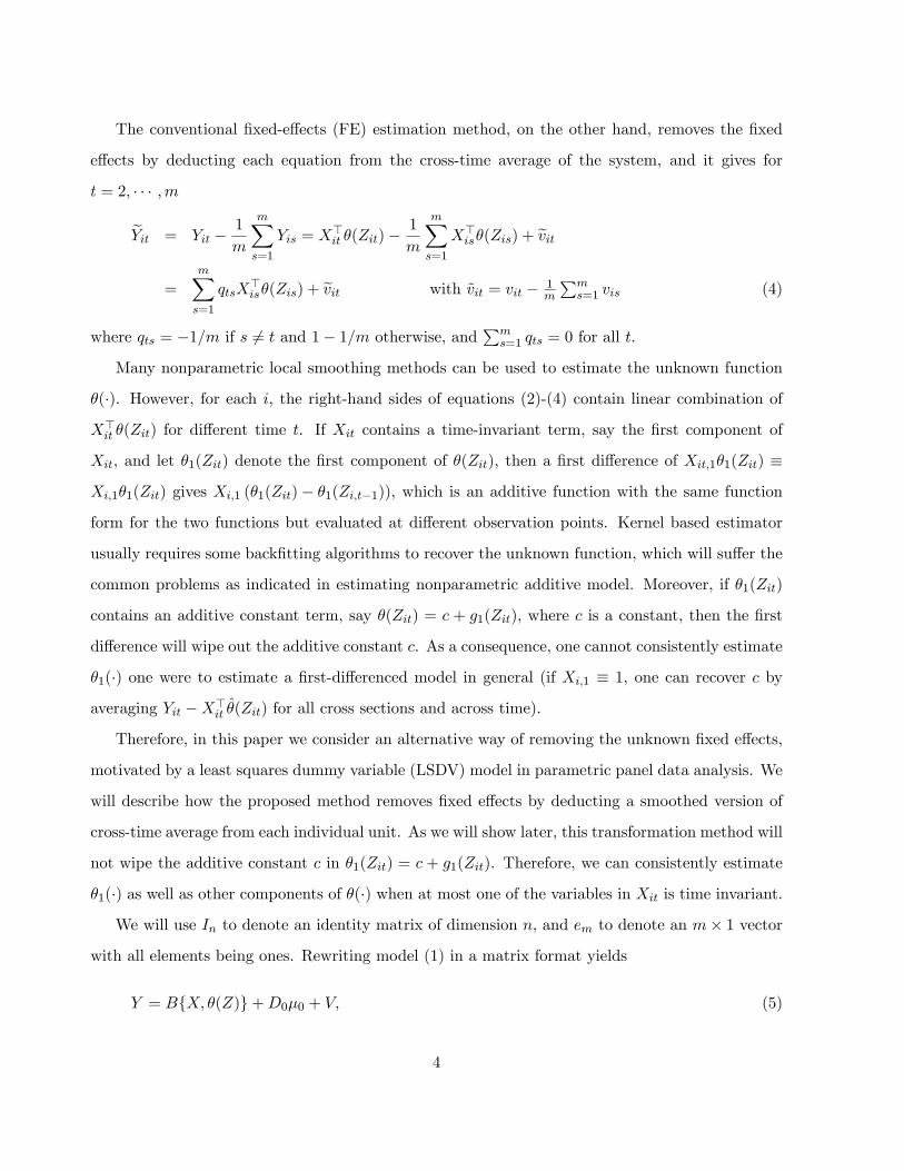
The conventional �xed-e�ects (FE) estimation method, on the other hand, removes the �xed

e�ects by deducting each equation from the cross-time average of the system, and it gives for

t = 2; � � � ;m

eYit = Yit �1

m

mXs=1

Yis = X>it �(Zit)�

1

m

mXs=1

X>is�(Zis) + evit

=

mXs=1

qtsX>is�(Zis) + evit with ~vit = vit � 1

m

Pms=1 vis (4)

where qts = �1=m if s 6= t and 1� 1=m otherwise, andPms=1 qts = 0 for all t.

Many nonparametric local smoothing methods can be used to estimate the unknown function

�(�). However, for each i, the right-hand sides of equations (2)-(4) contain linear combination of

X>it �(Zit) for di�erent time t. If Xit contains a time-invariant term, say the �rst component of

Xit, and let �1(Zit) denote the �rst component of �(Zit), then a �rst di�erence of Xit;1�1(Zit) �

Xi;1�1(Zit) gives Xi;1 (�1(Zit)� �1(Zi;t�1)), which is an additive function with the same function

form for the two functions but evaluated at di�erent observation points. Kernel based estimator

usually requires some back�tting algorithms to recover the unknown function, which will su�er the

common problems as indicated in estimating nonparametric additive model. Moreover, if �1(Zit)

contains an additive constant term, say �(Zit) = c + g1(Zit), where c is a constant, then the �rst

di�erence will wipe out the additive constant c. As a consequence, one cannot consistently estimate

�1(�) one were to estimate a �rst-di�erenced model in general (if Xi;1 � 1, one can recover c by

averaging Yit �X>it �(Zit) for all cross sections and across time).

Therefore, in this paper we consider an alternative way of removing the unknown �xed e�ects,

motivated by a least squares dummy variable (LSDV) model in parametric panel data analysis. We

will describe how the proposed method removes �xed e�ects by deducting a smoothed version of

cross-time average from each individual unit. As we will show later, this transformation method will

not wipe the additive constant c in �1(Zit) = c + g1(Zit). Therefore, we can consistently estimate

�1(�) as well as other components of �(�) when at most one of the variables in Xit is time invariant.

We will use In to denote an identity matrix of dimension n, and em to denote an m� 1 vector

with all elements being ones. Rewriting model (1) in a matrix format yields

Y = BfX; �(Z)g+D0�0 + V; (5)

4

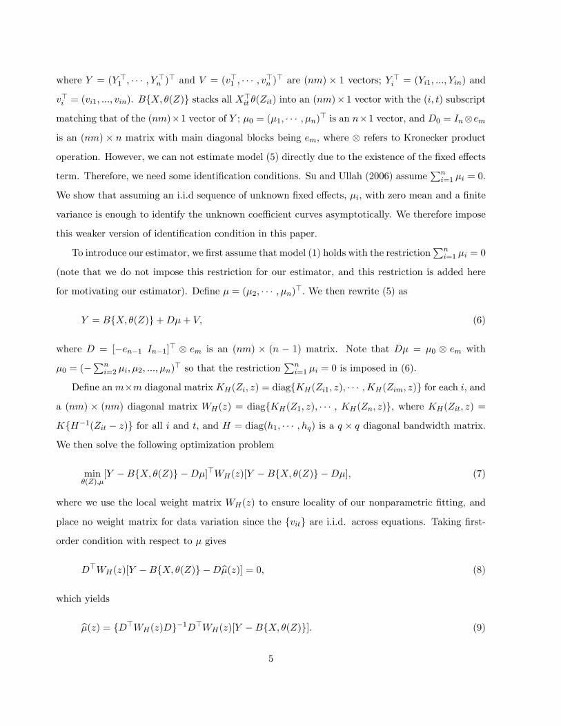
where Y = (Y >1 ; � � � ; Y >n )> and V = (v>1 ; � � � ; v>n )> are (nm) � 1 vectors; Y >i = (Yi1; :::; Yin) and

v>i = (vi1; :::; vin). BfX; �(Z)g stacks all X>it �(Zit) into an (nm)� 1 vector with the (i; t) subscript

matching that of the (nm)�1 vector of Y ; �0 = (�1; � � � ; �n)> is an n�1 vector, and D0 = Inem

is an (nm) � n matrix with main diagonal blocks being em, where refers to Kronecker product

operation. However, we can not estimate model (5) directly due to the existence of the �xed e�ects

term. Therefore, we need some identi�cation conditions. Su and Ullah (2006) assumePni=1 �i = 0.

We show that assuming an i.i.d sequence of unknown �xed e�ects, �i, with zero mean and a �nite

variance is enough to identify the unknown coe�cient curves asymptotically. We therefore impose

this weaker version of identi�cation condition in this paper.

To introduce our estimator, we �rst assume that model (1) holds with the restrictionPni=1 �i = 0

(note that we do not impose this restriction for our estimator, and this restriction is added here

for motivating our estimator). De�ne � = (�2; � � � ; �n)>: We then rewrite (5) as

Y = BfX; �(Z)g+D�+ V; (6)

where D = [�en�1 In�1]> em is an (nm) � (n � 1) matrix. Note that D� = �0 em with

�0 = (�Pni=2 �i; �2; :::; �n)

> so that the restrictionPni=1 �i = 0 is imposed in (6).

De�ne anm�m diagonal matrix KH(Zi; z) = diagfKH(Zi1; z); � � � ;KH(Zim; z)g for each i; and

a (nm) � (nm) diagonal matrix WH(z) = diagfKH(Z1; z); � � � ; KH(Zn; z)g, where KH(Zit; z) =

KfH�1(Zit � z)g for all i and t; and H = diag(h1; � � � ; hq) is a q � q diagonal bandwidth matrix.

We then solve the following optimization problem

min�(Z);�

[Y �BfX; �(Z)g �D�]>WH(z)[Y �BfX; �(Z)g �D�]; (7)

where we use the local weight matrix WH(z) to ensure locality of our nonparametric �tting, and

place no weight matrix for data variation since the fvitg are i.i.d. across equations. Taking �rst-

order condition with respect to � gives

D>WH(z)[Y �BfX; �(Z)g �Db�(z)] = 0; (8)

which yields

b�(z) = fD>WH(z)Dg�1D>WH(z)[Y �BfX; �(Z)g]: (9)

5

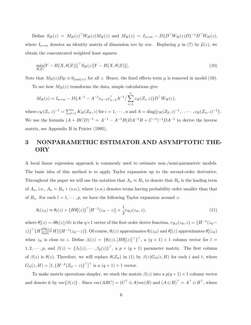
De�ne SH(z) = MH(z)>WH(z)MH(z) and MH(z) = In�m � DfD>WH(z)Dg�1D>WH(z),

where In�m denotes an identity matrix of dimension nm by nm. Replacing � in (7) by b�(z), weobtain the concentrated weighted least squares

min�(Z)

[Y �BfX; �(Z)g]>SH(z)[Y �BfX; �(Z)g]; (10)

Note that MH(z)D� � 0(nm)�1 for all z. Hence, the �xed e�ects term � is removed in model (10).

To see how MH(z) transforms the data, simple calculations give

MH(z) = In�m �DfA�1 �A�1en�1e>n�1A�1=nXi=1

cH(Zi; z)gD>WH(z);

where cH(Zi; z)�1 =

Pmt=1KH(Zit; z) for i = 1; � � � ; n andA = diagfcH(Z2; z)�1; : : � � � ; cH(Zn; z)�1g.

We use the formula (A + BCD)�1 = A�1 � A�1B(DA�1B + C�1)�1DA�1 to derive the inverse

matrix, see Appendix B in Poirier (1995).

3 NONPARAMETRIC ESTIMATORANDASYMPTOTIC THE-

ORY

A local linear regression approach is commonly used to estimate non-/semi-parametric models.

The basic idea of this method is to apply Taylor expansion up to the second-order derivative.

Throughout the paper we will use the notation that An � Bn to denote that Bn is the leading term

of An, i.e., An = Bn+(s:o:), where (s:o:) denotes terms having probability order smaller than that

of Bn. For each l = 1; � � � ; p; we have the following Taylor expansion around z:

�l(zit) � �l(z) + fH�0l(z)g>[H�1(zit � z)] +1

2rH;l(zit; z); (11)

where �0l(z) = @�l(z)=@z is the q�1 vector of the �rst order derive function, rH;l(zit; z) = fH�1(zit�

z)g>fH @2�l(z)@z@z>

HgfH�1(zit�z)g: Of course, �l(z) approximates �l(zit) and �0l(z) approximates �0l(zit)

when zit is close to z: De�ne �l(z) = f�l(z); [H�0l(z)]>g>; a (q + 1) � 1 column vector for l =

1; 2; � � � ; p; and �(z) = f�1(z); � � � ; �p(z)g>, a p � (q + 1) parameter matrix. The �rst column

of �(z) is �(z): Therefore, we will replace �(Zit) in (1) by �(z)Git(z;H) for each i and t; where

Git(z;H) = [1; fH�1(Zit � z)g>]> is a (q + 1)� 1 vector.

To make matrix operations simpler, we stack the matrix �(z) into a p(q+1)� 1 column vector

and denote it by vecf�(z)g . Since vec(ABC) = (C>A)vec(B) and (AB)> = A>B>; where

6

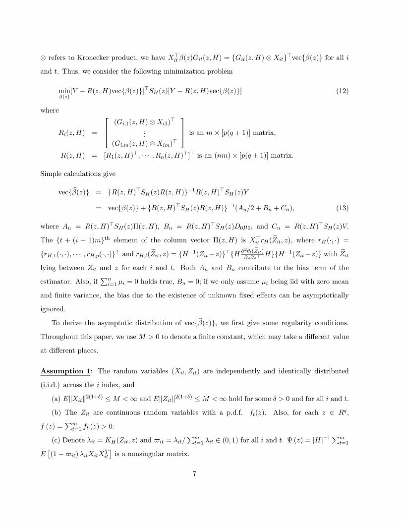
refers to Kronecker product, we have X>it �(z)Git(z;H) = fGit(z;H) Xitg>vecf�(z)g for all i

and t. Thus, we consider the following minimization problem

min�(z)

[Y �R(z;H)vecf�(z)g]>SH(z)[Y �R(z;H)vecf�(z)g] (12)

where

Ri(z;H) =

264 (Gi;1(z;H)Xi1)>...

(Gi;m(z;H)Xim)>

375 is an m� [p(q + 1)] matrix,

R(z;H) = [R1(z;H)>; � � � ; Rn(z;H)>]> is an (nm)� [p(q + 1)] matrix.

Simple calculations give

vecfb�(z)g = fR(z;H)>SH(z)R(z;H)g�1R(z;H)>SH(z)Y

= vecf�(z)g+ fR(z;H)>SH(z)R(z;H)g�1(An=2 +Bn + Cn); (13)

where An = R(z;H)>SH(z)�(z;H), Bn = R(z;H)>SH(z)D0�0, and Cn = R(z;H)>SH(z)V:

The ft + (i � 1)mgth element of the column vector �(z;H) is X>it rH(

eZit; z); where rH(�; �) =frH;1(�; �); � � � ; rH;p(�; �)g> and rH;l( eZit; z) = fH�1(Zit�z)g>fH @2�l( eZit)

@z@z>HgfH�1(Zit�z)g with eZit

lying between Zit and z for each i and t. Both An and Bn contribute to the bias term of the

estimator. Also, ifPni=1 �i = 0 holds true, Bn = 0; if we only assume �i being iid with zero mean

and �nite variance, the bias due to the existence of unknown �xed e�ects can be asymptotically

ignored.

To derive the asymptotic distribution of vecfb�(z)g, we �rst give some regularity conditions.Throughout this paper, we use M > 0 to denote a �nite constant, which may take a di�erent value

at di�erent places.

Assumption 1: The random variables (Xit; Zit) are independently and identically distributed

(i.i.d.) across the i index, and

(a) EkXitk2(1+�) �M <1 and EkZitk2(1+�) �M <1 hold for some � > 0 and for all i and t.

(b) The Zit are continuous random variables with a p.d.f. ft(z). Also, for each z 2 Rq,

f (z) =Pmt=1 ft (z) > 0.

(c) Denote �it = KH(Zit; z) and $it = �it=Pmt=1 �it 2 (0; 1) for all i and t. (z) = jHj

�1Pmt=1

E�(1�$it)�itXitXT

it

�is a nonsingular matrix.

7

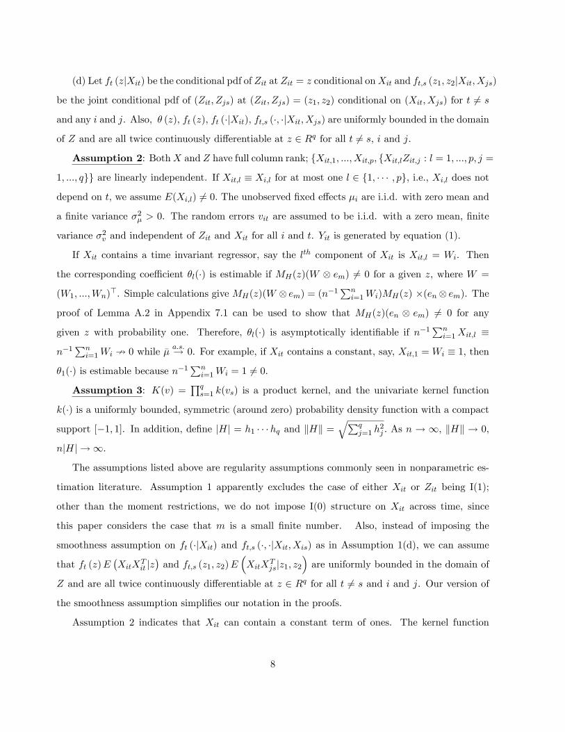
(d) Let ft (zjXit) be the conditional pdf of Zit at Zit = z conditional onXit and ft;s (z1; z2jXit; Xjs)

be the joint conditional pdf of (Zit; Zjs) at (Zit; Zjs) = (z1; z2) conditional on (Xit; Xjs) for t 6= s

and any i and j. Also, � (z), ft (z), ft (�jXit), ft;s (�; �jXit; Xjs) are uniformly bounded in the domain

of Z and are all twice continuously di�erentiable at z 2 Rq for all t 6= s, i and j.

Assumption 2: BothX and Z have full column rank; fXit;1; :::; Xit;p; fXit;lZit;j : l = 1; :::; p; j =

1; :::; qgg are linearly independent. If Xit;l � Xi;l for at most one l 2 f1; � � � ; pg, i.e., Xi;l does not

depend on t, we assume E(Xi;l) 6= 0: The unobserved �xed e�ects �i are i.i.d. with zero mean and

a �nite variance �2� > 0. The random errors vit are assumed to be i.i.d. with a zero mean, �nite

variance �2v and independent of Zit and Xit for all i and t. Yit is generated by equation (1).

If Xit contains a time invariant regressor, say the lth component of Xit is Xit;l = Wi. Then

the corresponding coe�cient �l(�) is estimable if MH(z)(W em) 6= 0 for a given z, where W =

(W1; :::;Wn)>. Simple calculations give MH(z)(W em) = (n�1

Pni=1Wi)MH(z) �(en em). The

proof of Lemma A.2 in Appendix 7.1 can be used to show that MH(z)(en em) 6= 0 for any

given z with probability one. Therefore, �l(�) is asymptotically identi�able if n�1Pni=1Xit;l �

n�1Pni=1Wi 9 0 while ��

a:s:! 0. For example, if Xit contains a constant, say, Xit;1 =Wi � 1; then

�1(�) is estimable because n�1Pni=1Wi = 1 6= 0.

Assumption 3: K(v) =Qqs=1 k(vs) is a product kernel, and the univariate kernel function

k(�) is a uniformly bounded, symmetric (around zero) probability density function with a compact

support [�1; 1]. In addition, de�ne jHj = h1 � � �hq and kHk =qPq

j=1 h2j : As n ! 1, kHk ! 0,

njHj ! 1.

The assumptions listed above are regularity assumptions commonly seen in nonparametric es-

timation literature. Assumption 1 apparently excludes the case of either Xit or Zit being I(1);

other than the moment restrictions, we do not impose I(0) structure on Xit across time, since

this paper considers the case that m is a small �nite number. Also, instead of imposing the

smoothness assumption on ft (�jXit) and ft;s (�; �jXit; Xis) as in Assumption 1(d), we can assume

that ft (z)E�XitX

Tit jz�and ft;s (z1; z2)E

�XitX

Tjsjz1; z2

�are uniformly bounded in the domain of

Z and are all twice continuously di�erentiable at z 2 Rq for all t 6= s and i and j. Our version of

the smoothness assumption simpli�es our notation in the proofs.

Assumption 2 indicates that Xit can contain a constant term of ones. The kernel function

8

having a compact support in Assumption 3 is imposed for the sake of brevity of proof and can be

removed at the cost of lengthy proofs. Speci�cally, the Gaussian kernel is allowed.

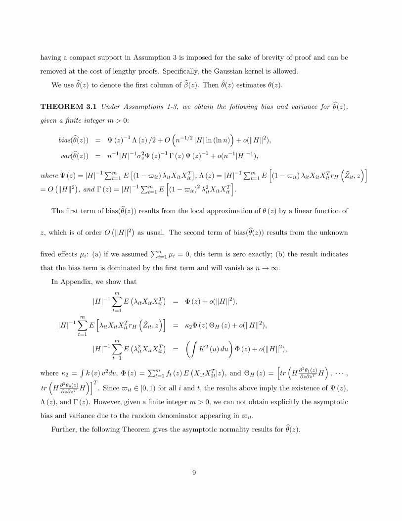
We use b�(z) to denote the �rst column of b�(z). Then �(z) estimates �(z).THEOREM 3.1 Under Assumptions 1-3, we obtain the following bias and variance for b�(z),given a �nite integer m > 0:

bias(b�(z)) = (z)�1 � (z) =2 +O�n�1=2 jHj ln (lnn)

�+ o(kHk2);

var(b�(z)) = n�1jHj�1�2v(z)�1 � (z) (z)�1 + o(n�1jHj�1);

where (z) = jHj�1Pmt=1 E

�(1�$it)�itXitXT

it

�, � (z) = jHj�1

Pmt=1E

h(1�$it)�itXitXT

it rH

�~Zit; z

�i= O

�kHk2

�, and � (z) = jHj�1

Pmt=1E

h(1�$it)2 �2itXitXT

it

i.

The �rst term of bias(b�(z)) results from the local approximation of � (z) by a linear function of

z, which is of order O�kHk2

�as usual. The second term of bias(b�(z)) results from the unknown

�xed e�ects �i: (a) if we assumedPni=1 �i = 0, this term is zero exactly; (b) the result indicates

that the bias term is dominated by the �rst term and will vanish as n!1.

In Appendix, we show that

jHj�1mXt=1

E��itXitX

Tit

�= �(z) + o(kHk2),

jHj�1mXt=1

Eh�itXitX

Tit rH

�~Zit; z

�i= �2� (z)�H (z) + o(kHk2),

jHj�1mXt=1

E��2itXitX

Tit

�=

�ZK2 (u) du

�� (z) + o(kHk2),

where �2 =Rk (v) v2dv, � (z) =

Pmt=1 ft (z)E

�X1tX

T1tjz�, and �H (z) =

htr�H @2�1(z)

@z@zTH�; � � � ;

tr�H@2�p(z)@z@zT

H�iT

. Since $it 2 [0; 1) for all i and t, the results above imply the existence of (z),

� (z), and � (z). However, given a �nite integer m > 0, we can not obtain explicitly the asymptotic

bias and variance due to the random denominator appearing in $it.

Further, the following Theorem gives the asymptotic normality results for b�(z).

9

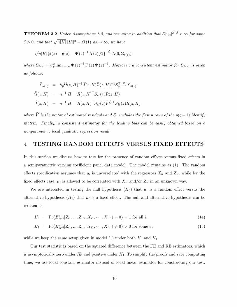
THEOREM 3.2 Under Assumptions 1-3, and assuming in addition that Ejvitj2+� <1 for some

� > 0, and thatpnjHjkHk2 = O (1) as !1, we havep

njHjfb�(z)� �(z)�(z)�1 � (z) =2g d! N(0;��(z));

where ��(z) = �2v limn!1(z)

�1 � (z) (z)�1. Moreover, a consistent estimator for ��(z) is given

as follows:

b��(z) = Spb(z;H)�1 bJ(z;H)b(z;H)�1S>p p! ��(z);b(z;H) = n�1jHj�1R(z;H)>SH(z)R(z;H)bJ(z;H) = n�1jHj�1R(z;H)>SH(z)bV bV >SH(z)R(z;H)where bV is the vector of estimated residuals and Sp includes the �rst p rows of the p(q+1) identify

matrix. Finally, a consistent estimator for the leading bias can be easily obtained based on a

nonparametric local quadratic regression result.

4 TESTING RANDOM EFFECTS VERSUS FIXED EFFECTS

In this section we discuss how to test for the presence of random e�ects versus �xed e�ects in

a semiparametric varying coe�cient panel data model. The model remains as (1). The random

e�ects speci�cation assumes that �i is uncorrelated with the regressors Xit and Zit, while for the

�xed e�ects case, �i is allowed to be correlated with Xit and/or Zit in an unknown way.

We are interested in testing the null hypothesis (H0) that �i is a random e�ect versus the

alternative hypothesis (H1) that �i is a �xed e�ect. The null and alternative hypotheses can be

written as

H0 : PrfE(�ijZi1; :::; Zim; Xi1; � � � ; Xim) = 0g = 1 for all i, (14)

H1 : PrfE(�ijZi1; :::; Zim; Xi1; � � � ; Xim) 6= 0g > 0 for some i , (15)

while we keep the same setup given in model (1) under both H0 and H1.

Our test statistic is based on the squared di�erence between the FE and RE estimators, which

is asymptotically zero under H0 and positive under H1: To simplify the proofs and save computing

time, we use local constant estimator instead of local linear estimator for constructing our test.

10

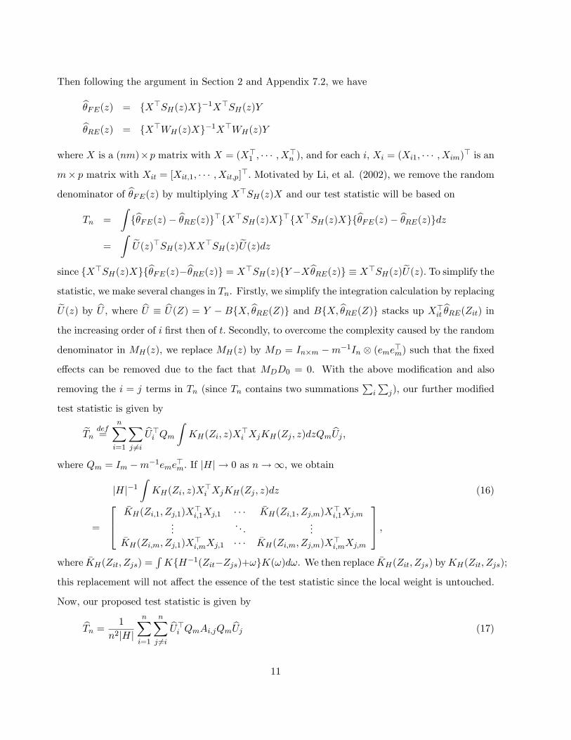
Then following the argument in Section 2 and Appendix 7.2, we have

b�FE(z) = fX>SH(z)Xg�1X>SH(z)Yb�RE(z) = fX>WH(z)Xg�1X>WH(z)Y

where X is a (nm)�p matrix with X = (X>1 ; � � � ; X>

n ); and for each i, Xi = (Xi1; � � � ; Xim)> is an

m� p matrix with Xit = [Xit;1; � � � ; Xit;p]>: Motivated by Li, et al. (2002), we remove the random

denominator of b�FE(z) by multiplying X>SH(z)X and our test statistic will be based on

Tn =

Zfb�FE(z)� b�RE(z)g>fX>SH(z)Xg>fX>SH(z)Xgfb�FE(z)� b�RE(z)gdz

=

Z eU(z)>SH(z)XX>SH(z)eU(z)dzsince fX>SH(z)Xgfb�FE(z)�b�RE(z)g = X>SH(z)fY �Xb�RE(z)g � X>SH(z)eU(z): To simplify thestatistic, we make several changes in Tn. Firstly, we simplify the integration calculation by replacingeU(z) by bU , where bU � bU(Z) = Y � BfX; b�RE(Z)g and BfX; b�RE(Z)g stacks up X>

itb�RE(Zit) in

the increasing order of i �rst then of t: Secondly, to overcome the complexity caused by the random

denominator in MH(z), we replace MH(z) by MD = In�m �m�1In (eme>m) such that the �xed

e�ects can be removed due to the fact that MDD0 = 0. With the above modi�cation and also

removing the i = j terms in Tn (since Tn contains two summationsPi

Pj), our further modi�ed

test statistic is given by

eTn def= nXi=1

Xj 6=i

bU>i Qm Z KH(Zi; z)X>i XjKH(Zj ; z)dzQm

bUj ;where Qm = Im �m�1eme>m: If jHj ! 0 as n!1, we obtain

jHj�1ZKH(Zi; z)X

>i XjKH(Zj ; z)dz (16)

=

264�KH(Zi;1; Zj;1)X

>i;1Xj;1 � � � �KH(Zi;1; Zj;m)X

>i;1Xj;m

.... . .

...�KH(Zi;m; Zj;1)X

>i;mXj;1 � � � �KH(Zi;m; Zj;m)X

>i;mXj;m

375 ,where �KH(Zit; Zjs) =

RKfH�1(Zit�Zjs)+!gK(!)d!. We then replace �KH(Zit; Zjs) byKH(Zit; Zjs);

this replacement will not a�ect the essence of the test statistic since the local weight is untouched.

Now, our proposed test statistic is given by

bTn = 1

n2jHj

nXi=1

nXj 6=i

bU>i QmAi;jQm bUj (17)

11

whereAi;j equals to the right-hand side of equation (16) after replacing �KH(Zit; Zjs) byKH(Zit; Zjs).

Finally, to remove the asymptotic bias term of the proposed test statistic, we calculate the leave-

one-unit-out random-e�ects estimator of �(Zit); that is, for a given pair of (i; j) in the double

summation of (17) with i 6= j, b�RE(Zit) is calculated without using the observations on the jth-unit, f(Xjt; Zjt; Yjt)gmt=1 and b�RE(Zjt) is calculated without using the observations on the ith-unit.

We present the asymptotic properties of this test below and delay the proofs to Appendix 7.3.

THEOREM 4.1 Under Assumptions 1-3, and ft (z) has a compact support S for all t, and

npjHj kHk4 ! 0 as n!1, then we have under H0 that

Jn = npjHj bTn=b�0 d! N(0; 1) (18)

where b�20 = 2n2jHj

Pni=1

Pnj 6=i(

bV >i QmAi;jQm bVj)2 is a consistent estimator of�20 = 4(1� 1=m)2�4v

ZK2(u)du

mXt=2

t�1Xs=1

Ehft(Z1s)(X

>1sX2t)

2i,

where bVit = Yit � X>itb�FE(Zit) � b�i and for each pair of (i; j), i 6= j, b�FE(Zit) is a leave-two-

unit-out FE estimator without using the observations from the ith and jth units and b�i = �Yi �

m�1Pmt=1X

>itb�FE(Zit). Under H1, Pr[Jn > Bn] ! 1 as n ! 1, where Bn is any nonstochastic

sequence with Bn = o(npjHj).

Assuming that ft (z) has a compact support S for all t is to simplify the proof of supz2S jjb�RE(z)�� (z) jj = op (1) as n ! 1; otherwise, some trimming procedure has to be placed to show the

uniform convergence result and the consistency of b�20 as an estimator of �20. Theorem 4.1 states

that the test statistic Jn = npjHj bTn=b�0 is a consistent test for testing H0 against H1. It is a

one-sided test. If Jn is greater than the critical values from the standard normal distribution, we

reject the null hypothesis at the corresponding signi�cance levels.

5 MONTE CARLO SIMULATIONS

In this section we report some Monte Carlo simulation results to examine the �nite sample perfor-

mance of the proposed estimator. The following data generating process is used:

Yit = �1(Zit) + �2(Zit)Xit + �i + vit; (19)

12

where �1(z) = 1 + z + z2, �2(z) = sin(z�), Zit = wit + wi;t�1, wit is i.i.d. uniformly distributed in

[0; �=2], Xit = 0:5Xi;t�1 + �it, �it is i.i.d. N(0; 1). In addition, �i = c0 �Zi� + ui for i = 2; � � � ; n with

c0 = 0; 0:5; and 1.0, ui is i.i.d. N(0; 1):When c0 6= 0, �i and Zit are correlated; we use c0 to control

the correlation between �i and �Zi� = m�1Pmt=1 Zit. Moreover, vit is i.i.d. N(0; 1), wit, �it, ui and

vit are independent of each other.

We report estimation results for both the proposed �xed-e�ects (FE) estimator and the random-

e�ects (RE) estimator, see Appendix 7.2 for the asymptotic results of the RE estimator. To learn

how the two estimators perform when we have �xed-e�ects model and when we have random-e�ects

model, we use the integrated squared error as a standard measure of estimation accuracy:

ISE(b�l) = Z fb�l(z)� �l(z)g2f(z)dz; (20)

which can be approximated by the average mean squared error

AMSE(b�l) = (nm)�1 nXi=1

mXt=1

[b�l(Zit)� �l(Zit)]2for l = 1; 2. In Table 1 we present the average value of AMSE(b�l) from 1000 Monte Carlo

experiments. We choose m = 3 and n = 50, 100, and 200.

Since the bias and variance of the proposed FE estimator do not depend on the values of the

�xed e�ects, our estimates are the same for di�erent values of c0; however, it is not true under the

random-e�ects model. Therefore, the results derived from the FE estimator are only reported once

in Table 1 since it is invariant to di�erent values of c0.

It is well-known that the performance of non/semiparametric models depends on the choice of

bandwidth. Therefore, we propose a leave-one-unit-out cross validation method to automatically

select the optimal bandwidth for estimating both the FE and RE models. Speci�cally, when

estimating �(�) at a point Zit; we remove f(Xit; Yit; Zit)gmt=1 from the data and only use the rest

of (n � 1)m observations to calculate b�(�i)(Zit). In computing the RE estimate, the leave-one-unit-out cross validation method is just a trivial extension of the conventional leave-one-out cross

validation method. The conventional leave-one-out method fails to provide satisfying result due to

the existence of unknown �xed e�ects. Therefore, when calculating the FE estimator, we use the

13

following modi�ed leave-one-unit-out cross validation method:

bHopt = argminH[Y �BfX; b�(�1)(Z)g]>M>

DMD[Y �BfX; b�(�1)(Z)g]; (21)

where MD = In�m � m�1In (eme>m) satis�es MDD0 = 0; this is used to remove the unknown

�xed e�ects. In addition, BfX; b�(�1)(Z)g stacks up X>itb�(�i)(Zit) in the increasing order of i �rst

then of t. Simple calculations give

[Y �BfX; b�(�1)(Z)g]>M>DMD[Y �BfX; b�(�1)(Z)g]

= [BfX; �(Z)g �BfX; b�(�1)(Z)g]>M>DMD[BfX; �(Z)g �BfX; b�(�1)(Z)g]

+2[BfX; �(Z)g �BfX; b�(�1)(Z)g]>M>DMDV + V

>MDMDV; (22)

where the last term does not depend on the bandwidth. If vit is independent of the fXjs; Zjsg for all

i, j, s and t, or (Xit; Zit) is strictly exogenous variable, then the second term has zero expectation

because the linear transformation matrix MD removes a cross-time not cross-sectional average

from each variable, e.g. eYit = Yit �m�1Pms=1 Yis for all i and t. Therefore, the �rst term is the

dominant term in large samples and (21) is used to �nd an optimal smoothing matrix minimizing

a weighted mean squared error of fb�(Zit)g: Of course, we could use other weight matrices in (21)instead of MD as long as the weight matrices can remove the �xed e�ects and do not trigger a

non-zero expectation of the second term in (22).

Table 1 shows that the RE estimator performs better than the FE estimator when the true

model is a random e�ects model. However, the FE estimator performs much better than the RE

estimator when the true model is a �xed-e�ects model. This is expected since the RE estimator

is inconsistent when the true model is the �xed e�ects model. Therefore, our simulation results

indicate that a test for random e�ects against �xed e�ects will be always in demand when we

analyze panel data models. In Table 2 we report simulation results of the proposed nonparametric

test of random e�ects against �xed e�ects.

For the selection of the bandwidth h, for univariate case, Theorem 4.1 indicates that h ! 0,

nh!1, and nh9=2 ! 0 as n!1; if we take h � n��; Theorem 4.1 requires � 2 (29 ; 1): To ful�ll

both conditions nh ! 1 and nh9=2 ! 0 as n ! 1, we use � = 2=7. Therefore, in producing

Table 2, we use h = c(nm)�2=7b�z to calculate the RE estimator with c taking a value from :8 , 1:0,

and 1:2. Since the computation is very time consuming, we only report results for n = 50 and 100.

14

With m = 3, the e�ective sample size is 150 and 300, which is small but moderate sample size.

Although the bandwidth chosen this way may not be optimal, the results in Tables 2, 3, and 4 show

that the proposed test statistic is not very sensitive to the choice of h when c changes and that a

moderate size distortion and decent power are consistent with the �ndings in the nonparametric

tests literature. We conjecture that some bootstrap procedures can be used to reduce the size

distortion in �nite samples. We will leave this as a future research topic.

6 CONCLUSION

In this paper we proposed a local linear least squares method to estimate a �xed e�ects varying

coe�cient panel data model when the number of observations across time is �nite; a data-driven

method was introduced to automatically �nd the optimal bandwidth for the proposed FE estimator.

In addition, we introduced a new test statistic to test for a random e�ects model against a �xed

e�ects model. Monte Carlo simulations indicate that the proposed estimator and test statistic have

good �nite sample performance.

7 APPENDIX

7.1 Proof of Theorem 3.1

To make our mathematical formula short, we introduce some simpli�ed notations �rst: for each i

and t; �it = KH (Zit; z) and cH (Zi; z)�1 =

Pmt=1 �it, and for any positive integers i; j; t; s

[�]it;js = Git (z;H)GTjs (z;H) =

266641 Gjs1 � � � GjsqGit1 Git1Gjs1 � � � Git1Gjsq...

.... . .

...Gitq GitqGjs1 � � � GitqGjsq

37775=

"1

�H�1 (Zjs � z)

�TH�1 (Zit � z) H�1 (Zit � z)

�H�1 (Zjs � z)

�T#

(A.1)

where the (l + 1)th element of Gjs (z;H) is Gjsl = (Zjsl � zl) =hl; l = 1; � � � ; q. Simple calculations

show that

[�]i1t1;i2t2 [�]j1s1;j2s2 =

0@1 + qXj=1

Gj1s1jGi2t2j

1A [�]i1t1;j2s2 ;Ri (z;H)

T KH (Zi; z) emeTmKH (Zj ; z)Rj (z;H) =

mXt=1

mXs=1

�it�js [�]it;js �XitX

Tjs

�15

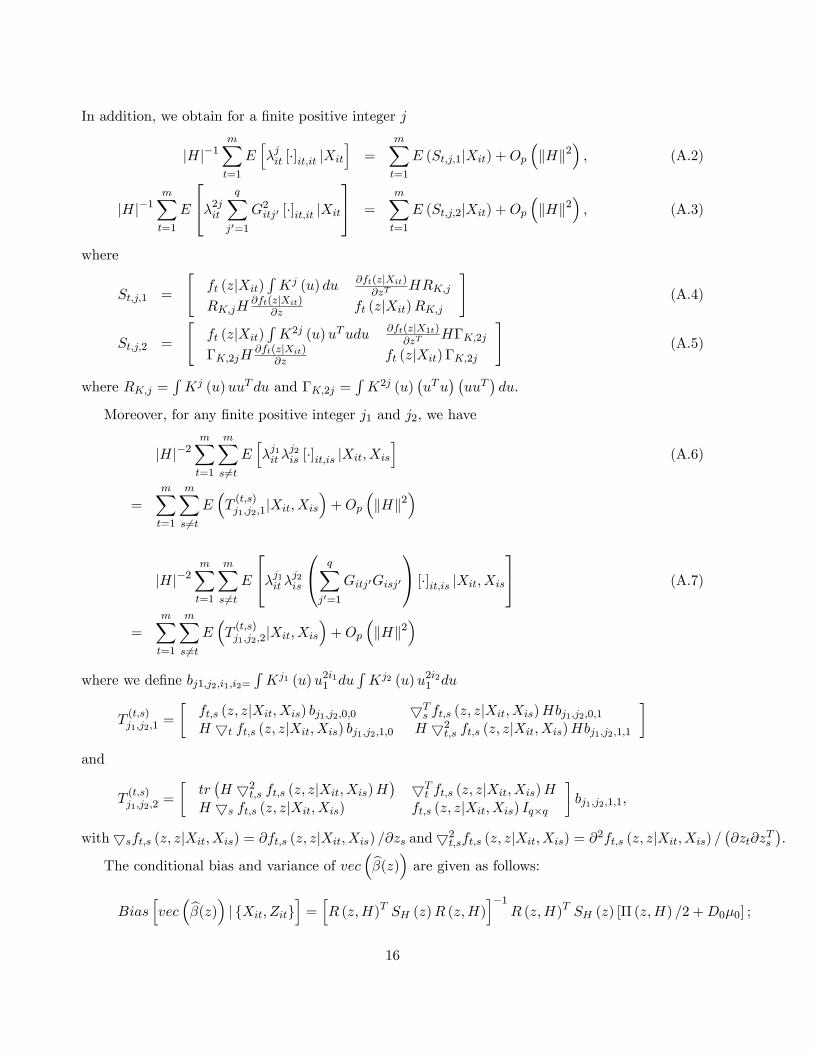
In addition, we obtain for a �nite positive integer j

jHj�1mXt=1

Eh�jit [�]it;it jXit

i=

mXt=1

E (St;j;1jXit) +Op�kHk2

�; (A.2)

jHj�1mXt=1

E

24�2jit qXj0=1

G2itj0 [�]it;it jXit

35 =mXt=1

E (St;j;2jXit) +Op�kHk2

�; (A.3)

where

St;j;1 =

"ft (zjXit)

RKj (u) du @ft(zjXit)

@zTHRK;j

RK;jH@ft(zjXit)

@z ft (zjXit)RK;j

#(A.4)

St;j;2 =

"ft (zjXit)

RK2j (u)uTudu @ft(zjX1t)

@zTH�K;2j

�K;2jH@ft(zjXit)

@z ft (zjXit) �K;2j

#(A.5)

where RK;j =RKj (u)uuTdu and �K;2j =

RK2j (u)

�uTu

� �uuT

�du.

Moreover, for any �nite positive integer j1 and j2; we have

jHj�2mXt=1

mXs 6=t

Eh�j1it �

j2is [�]it;is jXit; Xis

i(A.6)

=mXt=1

mXs 6=t

E�T(t;s)j1;j2;1

jXit; Xis�+Op

�kHk2

�

jHj�2mXt=1

mXs 6=t

E

24�j1it �j2is0@ qXj0=1

Gitj0Gisj0

1A [�]it;is jXit; Xis35 (A.7)

=

mXt=1

mXs 6=t

E�T(t;s)j1;j2;2

jXit; Xis�+Op

�kHk2

�where we de�ne bj1;j2;i1;i2=

RKj1 (u)u2i11 du

RKj2 (u)u2i21 du

T(t;s)j1;j2;1

=

�ft;s (z; zjXit; Xis) bj1;j2;0;0 5T

s ft;s (z; zjXit; Xis)Hbj1;j2;0;1H 5t ft;s (z; zjXit; Xis) bj1;j2;1;0 H 52

t;s ft;s (z; zjXit; Xis)Hbj1;j2;1;1

�and

T(t;s)j1;j2;2

=

�tr�H 52

t;s ft;s (z; zjXit; Xis)H�

5Tt ft;s (z; zjXit; Xis)H

H 5s ft;s (z; zjXit; Xis) ft;s (z; zjXit; Xis) Iq�q

�bj1;j2;1;1;

with5sft;s (z; zjXit; Xis) = @ft;s (z; zjXit; Xis) =@zs and52t;sft;s (z; zjXit; Xis) = @2ft;s (z; zjXit; Xis) =

�@zt@z

Ts

�.

The conditional bias and variance of vec�b�(z)� are given as follows:

Biashvec

�b�(z)� j fXit; Zitgi = hR (z;H)T SH (z)R (z;H)i�1R (z;H)T SH (z) [� (z;H) =2 +D0�0] ;16

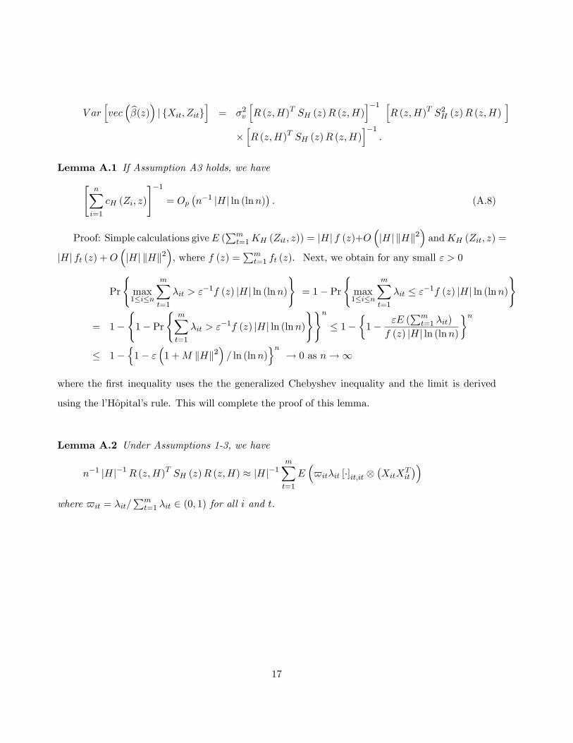
V arhvec

�b�(z)� j fXit; Zitgi = �2v

hR (z;H)T SH (z)R (z;H)

i�1 hR (z;H)T S2H (z)R (z;H)

i�hR (z;H)T SH (z)R (z;H)

i�1:

Lemma A.1 If Assumption A3 holds, we have"nXi=1

cH (Zi; z)

#�1= Op

�n�1 jHj ln (lnn)

�. (A.8)

Proof: Simple calculations give E (Pmt=1KH (Zit; z)) = jHj f (z)+O

�jHj kHk2

�andKH (Zit; z) =

jHj ft (z) +O�jHj kHk2

�, where f (z) =

Pmt=1 ft (z). Next, we obtain for any small " > 0

Pr

(max1�i�n

mXt=1

�it > "�1f (z) jHj ln (lnn)

)= 1� Pr

(max1�i�n

mXt=1

�it � "�1f (z) jHj ln (lnn))

= 1�(1� Pr

(mXt=1

�it > "�1f (z) jHj ln (lnn)

))n� 1�

�1� "E (

Pmt=1 �it)

f (z) jHj ln (lnn)

�n� 1�

n1� "

�1 +M kHk2

�= ln (lnn)

on! 0 as n!1

where the �rst inequality uses the the generalized Chebyshev inequality and the limit is derived

using the l'Hopital's rule. This will complete the proof of this lemma.

Lemma A.2 Under Assumptions 1-3, we have

n�1 jHj�1R (z;H)T SH (z)R (z;H) � jHj�1mXt=1

E�$it�it [�]it;it

�XitX

Tit

��where $it = �it=

Pmt=1 �it 2 (0; 1) for all i and t.

17

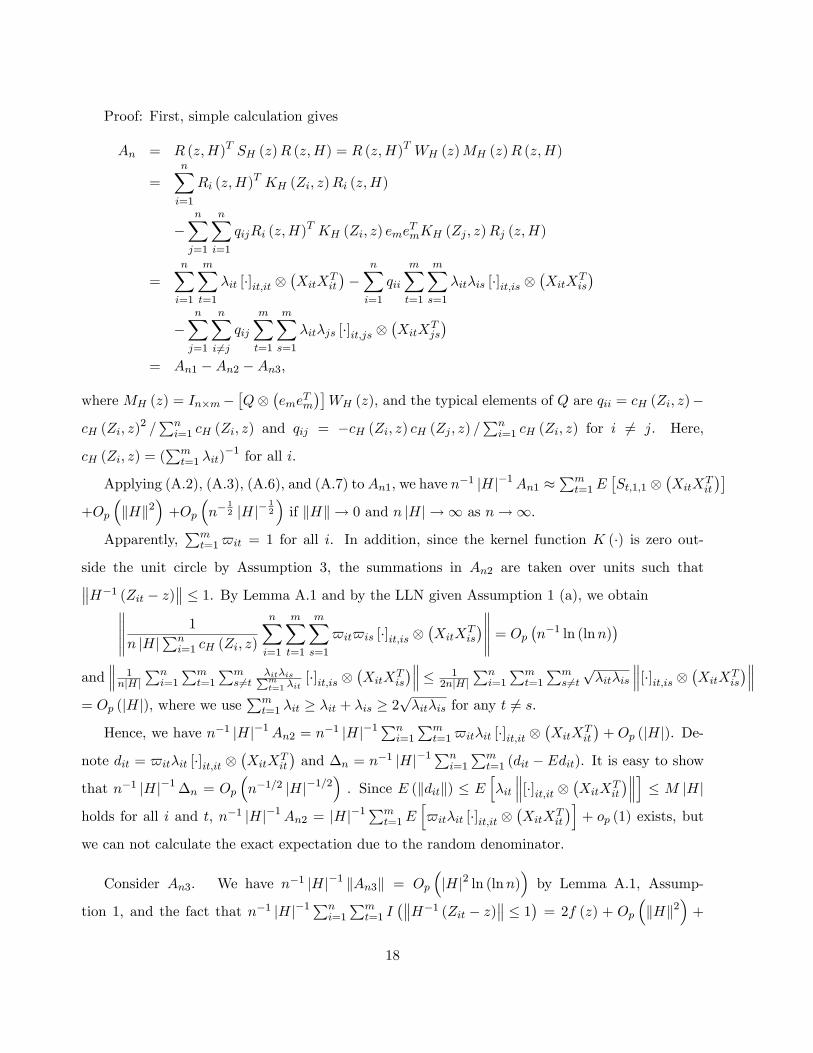
Proof: First, simple calculation gives

An = R (z;H)T SH (z)R (z;H) = R (z;H)T WH (z)MH (z)R (z;H)

=nXi=1

Ri (z;H)T KH (Zi; z)Ri (z;H)

�nXj=1

nXi=1

qijRi (z;H)T KH (Zi; z) eme

TmKH (Zj ; z)Rj (z;H)

=nXi=1

mXt=1

�it [�]it;it �XitX

Tit

��

nXi=1

qii

mXt=1

mXs=1

�it�is [�]it;is �XitX

Tis

��

nXj=1

nXi6=j

qij

mXt=1

mXs=1

�it�js [�]it;js �XitX

Tjs

�= An1 �An2 �An3;

where MH (z) = In�m��Q

�eme

Tm

��WH (z), and the typical elements of Q are qii = cH (Zi; z)�

cH (Zi; z)2 =Pni=1 cH (Zi; z) and qij = �cH (Zi; z) cH (Zj ; z) =

Pni=1 cH (Zi; z) for i 6= j. Here,

cH (Zi; z) = (Pmt=1 �it)

�1 for all i.

Applying (A.2), (A.3), (A.6), and (A.7) toAn1, we have n�1 jHj�1An1 �

Pmt=1E

�St;1;1

�XitX

Tit

��+Op

�kHk2

�+Op

�n�

12 jHj�

12

�if kHk ! 0 and n jHj ! 1 as n!1.

Apparently,Pmt=1$it = 1 for all i. In addition, since the kernel function K (�) is zero out-

side the unit circle by Assumption 3, the summations in An2 are taken over units such that H�1 (Zit � z) � 1. By Lemma A.1 and by the LLN given Assumption 1 (a), we obtain 1

n jHjPni=1 cH (Zi; z)

nXi=1

mXt=1

mXs=1

$it$is [�]it;is �XitX

Tis

� = Op �n�1 ln (lnn)�and

1njHj

Pni=1

Pmt=1

Pms 6=t

�it�isPmt=1 �it

[�]it;is �XitX

Tis

� � 12njHj

Pni=1

Pmt=1

Pms 6=tp�it�is

[�]it;is �XitXTis

� = Op (jHj), where we use

Pmt=1 �it � �it + �is � 2

p�it�is for any t 6= s.

Hence, we have n�1 jHj�1An2 = n�1 jHj�1Pni=1

Pmt=1$it�it [�]it;it

�XitX

Tit

�+ Op (jHj). De-

note dit = $it�it [�]it;it �XitX

Tit

�and �n = n

�1 jHj�1Pni=1

Pmt=1 (dit � Edit). It is easy to show

that n�1 jHj�1�n = Op�n�1=2 jHj�1=2

�. Since E (kditk) � E

h�it

[�]it;it �XitXTit

� i � M jHj

holds for all i and t, n�1 jHj�1An2 = jHj�1Pmt=1E

h$it�it [�]it;it

�XitX

Tit

�i+ op (1) exists, but

we can not calculate the exact expectation due to the random denominator.

Consider An3. We have n�1 jHj�1 kAn3k = Op

�jHj2 ln (lnn)

�by Lemma A.1, Assump-

tion 1, and the fact that n�1 jHj�1Pni=1

Pmt=1 I

� H�1 (Zit � z) � 1� = 2f (z) + Op

�kHk2

�+

18

Op

�n�1=2 jHj�1=2

�.

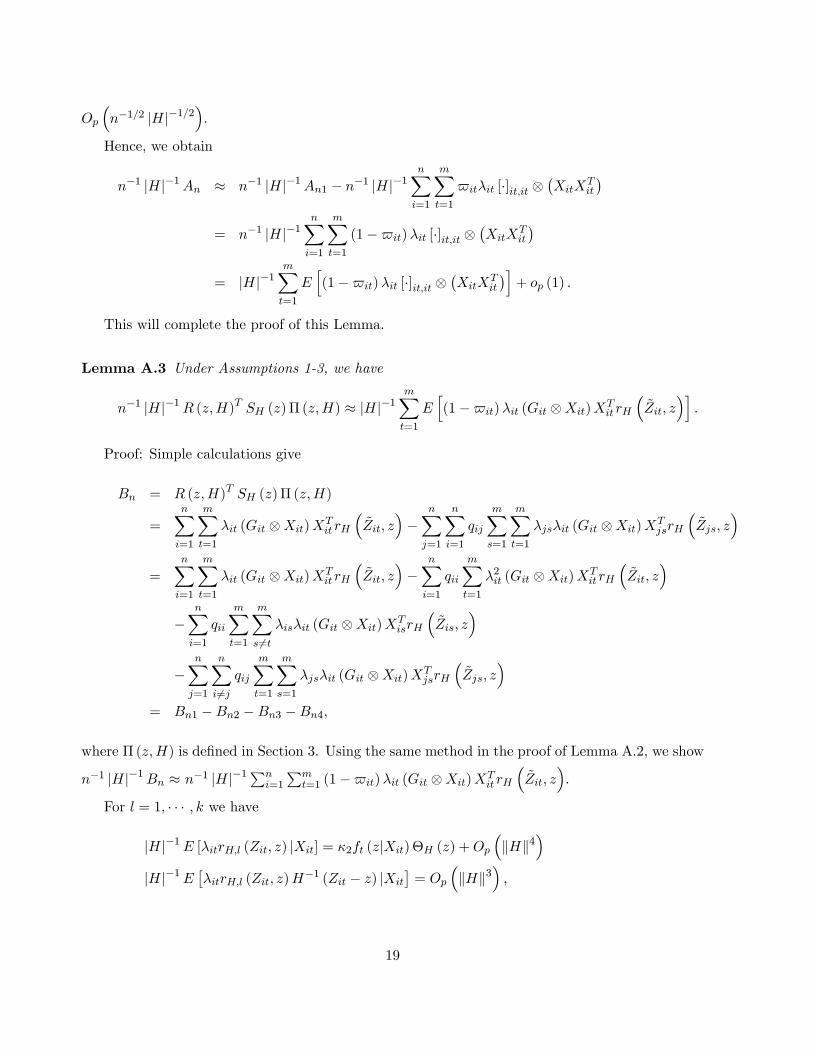
Hence, we obtain

n�1 jHj�1An � n�1 jHj�1An1 � n�1 jHj�1nXi=1

mXt=1

$it�it [�]it;it �XitX

Tit

�= n�1 jHj�1

nXi=1

mXt=1

(1�$it)�it [�]it;it �XitX

Tit

�= jHj�1

mXt=1

Eh(1�$it)�it [�]it;it

�XitX

Tit

�i+ op (1) :

This will complete the proof of this Lemma.

Lemma A.3 Under Assumptions 1-3, we have

n�1 jHj�1R (z;H)T SH (z)� (z;H) � jHj�1mXt=1

Eh(1�$it)�it (Git Xit)XT

it rH

�~Zit; z

�i:

Proof: Simple calculations give

Bn = R (z;H)T SH (z)� (z;H)

=nXi=1

mXt=1

�it (Git Xit)XTit rH

�~Zit; z

��

nXj=1

nXi=1

qij

mXs=1

mXt=1

�js�it (Git Xit)XTjsrH

�~Zjs; z

�=

nXi=1

mXt=1

�it (Git Xit)XTit rH

�~Zit; z

��

nXi=1

qii

mXt=1

�2it (Git Xit)XTit rH

�~Zit; z

��

nXi=1

qii

mXt=1

mXs 6=t

�is�it (Git Xit)XTisrH

�~Zis; z

��

nXj=1

nXi6=j

qij

mXt=1

mXs=1

�js�it (Git Xit)XTjsrH

�~Zjs; z

�= Bn1 �Bn2 �Bn3 �Bn4;

where � (z;H) is de�ned in Section 3. Using the same method in the proof of Lemma A.2, we show

n�1 jHj�1Bn � n�1 jHj�1Pni=1

Pmt=1 (1�$it)�it (Git Xit)XT

it rH

�~Zit; z

�.

For l = 1; � � � ; k we have

jHj�1E [�itrH;l (Zit; z) jXit] = �2ft (zjXit)�H (z) +Op�kHk4

�jHj�1E

��itrH;l (Zit; z)H

�1 (Zit � z) jXit�= Op

�kHk3

�;

19

and E�n�1 jHj�1Bn1

��n�2 [� (z)�H (z)]

T ; O�kHk3

�oT, where

�H (z) =

�tr

�H@2�1 (z)

@z@zTH

�; � � � ; tr

�H@2�k (z)

@z@zTH

��T:

Similarly we can show that V ar�n�1 jHj�1Bn1

�= O

�n�1 jHj�1 kHk4

�if E

� XitXTisXitX

Tis

� <M <1 for all t and s.

In addition, it is easy to show that n�1 jHj�1Pni=1

Pmt=1$it�it (Git Xit)XT

it rH

�~Zit; z

�=

n�1 jHj�1Pni=1

Pmt=1E

h$it�it (Git Xit)XT

it rH

�~Zit; z

�i+Op

�n�1=2 jHj�1=2 kHk2

�, where

jHj�1Pmt=1E

h$it�it (Git Xit)XT

it rH

�~Zit; z

�i� jHj�1

Pmt=1E

h�it

(Git Xit)XTit rH

�~Zit; z

� i�M kHk2 <1 for all i and t.

This will complete the proof of this lemma.

Lemma A.4 Under Assumptions 1-3, we have

n�1 jHj�1R (z;H)T SH (z)D0�0 = Op�n�1=2 jHj ln (lnn)

�.

Proof: Simple calculations give MH(z)D0�0 = ��MH(z) (en em), where �� = n�1Pni=1 �i. It

follows that

Cn = R (z;H)T SH (z)D0�0 = ��R (z;H)T SH (z) (en em)

= ��nXi=1

mXt=1

RTi Kiem � ��nXj=1

mXt=1

�jt

!nXi=1

qijRTi Kiem

= ��nXi=1

mXt=1

�it (Git Xit)� ��nXj=1

mXt=1

�jt

!nXi=1

qij

mXt=1

�it (Git Xit)

= n��

24 nXi=1

mXt=1

�it

!�135�1 nXi=1

mXt=1

$it (Git Xit)

and we obtain n�1 jHj�1Cn = ��Op (jHj ln (lnn)) by (a) Lemma A.1, (b) for all l = 1; � � � ; q,

k ((Zit;l � zl) =h) = 0 if jZit;l � zlj > h by Assumption 3, (c) $it � 1, and (d) E kXitk1+� < M <1

for some � > 0 by Assumption 1. Since �i � iid�0; �2�

�, we have �� = Op

�n�1=2

�. It follows that

n�1 jHj�1Cn = Op�n�1=2 jHj ln (lnn)

�.

Lemma A.5 Under Assumptions 1-3, we have

n�1 jHj�1R (z;H)T S2H (z)R (z;H) � jHj�1

mXt=1

Eh(1�$it)2 �2it [�]it

�XitX

Tit

�i:

20

Proof: Simple calculations give

Dn = R (z;H)T S2H (z)R (z;H) = R (z;H)T WH (z)MH (z)MH (z)

T WH (z)R (z;H)

=nXi=1

Ri (z;H)T K2

H (Zi; z)Ri (z;H)� 2nXj=1

nXi=1

qjiRj (z;H)T K2

H (Zj ; z) emeTmKH (Zi; z)Ri (z;H)

+nXj=1

nXi=1

nXi0=1

qijqji0Ri (z;H)T KH (Zi; z) eme

TmK

2H (Zj ; z) eme

TmKH (Zi0 ; z)Ri0 (z;H)

= Dn1 � 2Dn2 +Dn3:

Using the same method in the proof of Lemma A.2, we show Dn �Pni=1

Pmt=1 (1�$it)

2 �2it [�]it;it�XitX

Tit

�. It is easy to show that n�1 jHj�1Dn1 = n�1 jHj�1

Pni=1

Pmt=1 �

2it [�]it;it

�XitX

Tit

�=Pm

t=1E�St;2;1

�XitX

Tit

��+Op

�kHk2

�+Op

�n�1=2 jHj�1=2

�.

Also, we obtain n�1 jHj�1Pni=1

Pmt=1 (1�$it)

2 �2it [�]it;it�XitX

Tit

�= { (z)+Op

�n�1=2 jHj�1=2

�,

where { (z) = jHj�1Pmt=1 E

h(1�$it)2 �2it [�]it;it

�XitX

Tit

�i� jHj�1

Pmt=1E

h�2it

[�]it;it �XitXTit

� i�M <1 for all i and t.

The four lemmas above are enough to give the result of Theorem 3.1. Moreover, applying

Liaponuov's CLT will give the result of Theorem 3.2. Since the proof is a rather standard procedure,

we drop the details for compactness of the paper.

7.2 Technical Sketch{Random E�ects Estimator

The RE estimator, �RE(�), is the solution to the following optimization problem:

min�(z)

[Y �R (z;H) vec (� (z))]T WH (z) [Y �R (z;H) vec (� (z))] ;

that is, we have

vec��RE (z)

�=

hR (z;H)T WH (z)R (z;H)

i�1R (z;H)T WH (z)Y

= vec (� (z)) +hR (z;H)T WH (z)R (z;H)

i�1 �~An=2 + ~Bn + ~Cn

�where ~An = R (z;H)

T WH (z)� (z;H), ~Bn = R (z;H)T WH (z)D0�0, and ~Cn = R (z;H)

T WH (z)V .

Its asymptotic properties are as follows.

21

Lemma A.6 Under Assumptions 1-3, and E�XitX

Tit jz�and E (�iXitjz) have continuous second-

order derivative at z 2 Rq. Also,pn jHj kHk2 = O (1) as n ! 1, and E

�jvitj2+�

�< 1 and

E�j�ij2+�

�< M <1 for all i and t and for some � > 0, we have under H0

pn jHj

�b�RE(z)� �(z)� �2�H (z) =2� d! N�0;��(z);RE

�; (A.9)

where �2 =Rk (v) v2dv, ��(z);RE =

��2� + �

2v

�� (z)�1

RK2 (u) du and � (z) =

Pmt=1 ft (z)E

�X1tX

T1tjz�.

Under H1, we have

Bias�b�RE(z)� = �(z)�1

mXt=1

ft (z)E (�1X1tjz) + o (1)

V ar��RE (z)

�= n�1 jHj�1 �2v� (z)

�1ZK2 (u) du (A.10)

where �H (z) is given in the proof of Lemma A.3.

Proof of Lemma A.6: First, we have the following decompositionpn jHj

h�RE (z)� �(z)

i=pn jHj

h�RE (z)� E

��RE (z)

�i+pn jHj

hE��RE (z)

�� �(z)

i;

where we can show that the �rst term converges to a normal distribution with mean zero by

Liaponuov's CLT (the details are dropped since it is a rather standard proof), and the second

term contributes to the asymptotic bias. Since it will cause no notational confusion, we drop the

subscription `RE'. Below, we use Biasi

n� (z)

oand V ari

n� (z)

oto denote the respective bias and

variance of �RE (z) under H0 if i = 0 and under H1 if i = 1.

First, under H0, the bias and variance of � (z) are as follows: Bias0

n� (z) j f(Xit; Zit)g

o=

Sp

hR (z;H)T WH (z)R (z;H)

i�1R (z;H)T WH (z)� (z;H) =2 and

V ar0

n� (z) j f(Xit; Zit)g

o= Sp

hR (z;H)T WH (z)R (z;H)

i�1 hR (z;H)T WH (z)V ar(UU

T )WH (z)R (z;H)i

�hR (z;H)T WH (z)R (z;H)

i�1STp :

It is simple to show that V ar(UUT ) = �2�In �eme

Tm

�+ �2vIn�m.

22

Next, underH1, we notice thatBias1

n� (z) j f(Xit; Zit)g

ois the sum ofBias0

n� (z) j f(Xit; Zit)g

oplus an additional term Sp

hR (z;H)T WH (z)R (z;H)

i�1R (z;H)T WH (z)D0�0, and that

V ar1

n� (z) j f(Xit; Zit)g

o= �2vSp

hR (z;H)T WH (z)R (z;H)

i�1 hR (z;H)T WH (z)

2R (z;H)i

�hR (z;H)T WH (z)R (z;H)

i�1STp .

Noting that R (z;H)T WH (z)R (z;H) is An1 in Lemma A.2 and that R (z;H)T WH (z)� (z;H)

is Bn1 in Lemma A.3, we have

Bias0

n� (z)

o= �2�H (z) =2 + o

�kHk2

�. (A.11)

In addition, under Assumptions 1-3, and E�j�ij2+�

�< M < 1 and E

�kXitk2+�

�< M < 1 for

all i and t and for some � > 0, we show that

n�1 jHj�1 SpR (z;H)T WH (z)D0�0 = n�1 jHj�1 Sp

nXi=1

�i

mXt=1

�it (Git Xit)

=mXt=1

ft (z)E (�1X1tjz) +Op�kHk2

�+Op

�(n jHj)�1=2

�; (A.12)

which is a non-zero constant plus a term of op(1) under H1. Combining (A.11) and (A.12), we

obtain (A.10). Hence, under H1, the bias of the RE estimator will not vanish as n!1, and this

leads to the inconsistency of the RE estimator under H1.

As for the asymptotic variance, we can easily show that under H0

V ar0

n� (z)

o= n�1 jHj�1

��2� + �

2v

�� (z)�1

ZK2 (u) du; (A.13)

and under H1, V ar1

n� (z)

o= n�1 jHj�1 �2v� (z)

�1 R K2 (u) du, where we have recognized that

R (z;H)T WH (z)2R (z;H) is Dn1 in Lemma A.5, and

��2� + �

2v

�R (z;H)T WH (z)

2R (z;H) is the

leading term of R (z;H)T WH (z)V ar(UUT )WH (z)R (z;H).

23

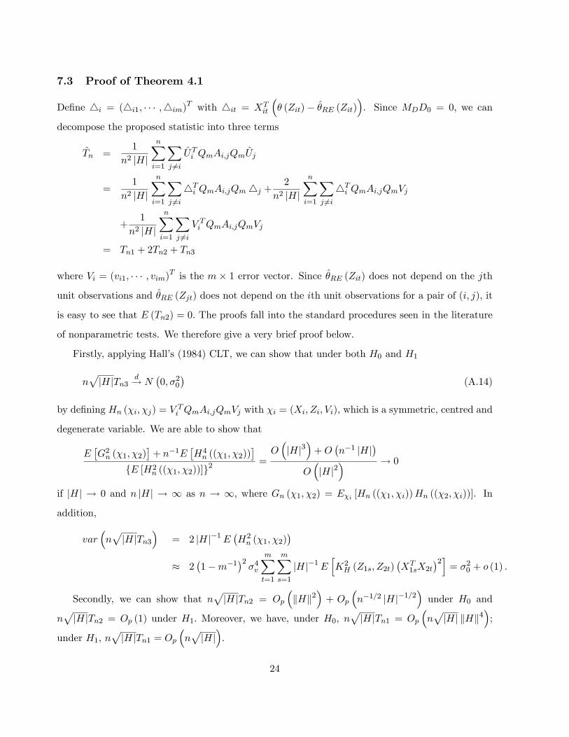
7.3 Proof of Theorem 4.1

De�ne 4i = (4i1; � � � ;4im)T with 4it = XT

it

�� (Zit)� �RE (Zit)

�. Since MDD0 = 0; we can

decompose the proposed statistic into three terms

Tn =1

n2 jHj

nXi=1

Xj 6=i

UTi QmAi;jQmUj

=1

n2 jHj

nXi=1

Xj 6=i

4Ti QmAi;jQm 4j +

2

n2 jHj

nXi=1

Xj 6=i

4Ti QmAi;jQmVj

+1

n2 jHj

nXi=1

Xj 6=i

V Ti QmAi;jQmVj

= Tn1 + 2Tn2 + Tn3

where Vi = (vi1; � � � ; vim)T is the m � 1 error vector. Since �RE (Zit) does not depend on the jth

unit observations and �RE (Zjt) does not depend on the ith unit observations for a pair of (i; j); it

is easy to see that E (Tn2) = 0: The proofs fall into the standard procedures seen in the literature

of nonparametric tests. We therefore give a very brief proof below.

Firstly, applying Hall's (1984) CLT, we can show that under both H0 and H1

npjHjTn3

d! N�0; �20

�(A.14)

by de�ning Hn (�i; �j) = VTi QmAi;jQmVj with �i = (Xi; Zi; Vi), which is a symmetric, centred and

degenerate variable. We are able to show that

E�G2n (�1; �2)

�+ n�1E

�H4n ((�1; �2))

�fE [H2

n ((�1; �2))]g2 =

O�jHj3

�+O

�n�1 jHj

�O�jHj2

� ! 0

if jHj ! 0 and n jHj ! 1 as n ! 1; where Gn (�1; �2) = E�i [Hn ((�1; �i))Hn ((�2; �i))]. In

addition,

var�npjHjTn3

�= 2 jHj�1E

�H2n (�1; �2)

�� 2

�1�m�1�2 �4v mX

t=1

mXs=1

jHj�1EhK2H (Z1s; Z2t)

�XT1sX2t

�2i= �20 + o (1) .

Secondly, we can show that npjHjTn2 = Op

�kHk2

�+ Op

�n�1=2 jHj�1=2

�under H0 and

npjHjTn2 = Op (1) under H1: Moreover, we have, under H0, n

pjHjTn1 = Op

�npjHj kHk4

�;

under H1, npjHjTn1 = Op

�npjHj�.

24

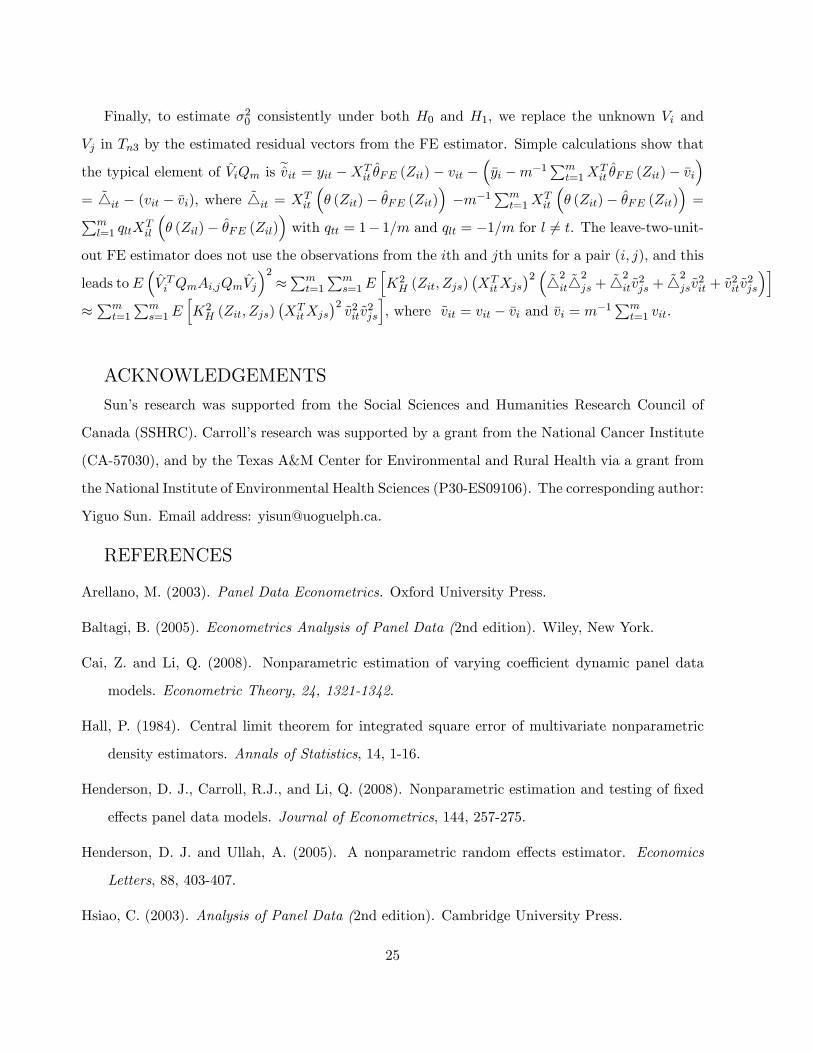
Finally, to estimate �20 consistently under both H0 and H1, we replace the unknown Vi and

Vj in Tn3 by the estimated residual vectors from the FE estimator. Simple calculations show that

the typical element of ViQm is evit = yit �XTit �FE (Zit) � vit �

��yi �m�1Pm

t=1XTit �FE (Zit)� �vi

�= ~4it � (vit � �vi), where ~4it = XT

it

�� (Zit)� �FE (Zit)

��m�1Pm

t=1XTit

�� (Zit)� �FE (Zit)

�=Pm

l=1 qltXTil

�� (Zil)� �FE (Zil)

�with qtt = 1� 1=m and qlt = �1=m for l 6= t. The leave-two-unit-

out FE estimator does not use the observations from the ith and jth units for a pair (i; j), and this

leads to E�V Ti QmAi;jQmVj

�2�Pmt=1

Pms=1E

hK2H (Zit; Zjs)

�XTitXjs

�2 � ~42it~42js +

~42it~v

2js +

~42js~v

2it + ~v

2it~v

2js

�i�Pmt=1

Pms=1E

hK2H (Zit; Zjs)

�XTitXjs

�2~v2it~v

2js

i, where ~vit = vit � �vi and �vi = m�1Pm

t=1 vit.

ACKNOWLEDGEMENTS

Sun's research was supported from the Social Sciences and Humanities Research Council of

Canada (SSHRC). Carroll's research was supported by a grant from the National Cancer Institute

(CA-57030), and by the Texas A&M Center for Environmental and Rural Health via a grant from

the National Institute of Environmental Health Sciences (P30-ES09106). The corresponding author:

Yiguo Sun. Email address: yisun@uoguelph.ca.

REFERENCES

Arellano, M. (2003). Panel Data Econometrics. Oxford University Press.

Baltagi, B. (2005). Econometrics Analysis of Panel Data (2nd edition). Wiley, New York.

Cai, Z. and Li, Q. (2008). Nonparametric estimation of varying coe�cient dynamic panel data

models. Econometric Theory, 24, 1321-1342.

Hall, P. (1984). Central limit theorem for integrated square error of multivariate nonparametric

density estimators. Annals of Statistics, 14, 1-16.

Henderson, D. J., Carroll, R.J., and Li, Q. (2008). Nonparametric estimation and testing of �xed

e�ects panel data models. Journal of Econometrics, 144, 257-275.

Henderson, D. J. and Ullah, A. (2005). A nonparametric random e�ects estimator. Economics

Letters, 88, 403-407.

Hsiao, C. (2003). Analysis of Panel Data (2nd edition). Cambridge University Press.

25

Li, Q. and Huang, C.J., Li, D. and Fu, T. (2002). Semiparametric smooth coe�cient models.

Journal of Business & Economic Statistics, 20, 412-422.

Li, Q. and Stengos, T. (1996). Semiparametric estimation of partially linear panel data models.

Journal of Econometrics, 71, 389-397.

Lin, D. Y. and Ying, Z. (2001). Semiparametric and nonparametric regression analysis of longitu-

dinal data (with discussion). Journal of the American Statistical Association, 96, 103-126.

Lin, X., and Carroll, R. J. (2000). Nonparametric function estimation for clustered data when the

predictor is measured without/with Error. Journal of the American Statistical Association, 95,

520-534.

Lin, X. and Carroll, R. J. (2001). Semiparametric regression for clustered data using generalized

estimation equations. Journal of the American Statistical Association, 96, 1045-1056.

Lin, X. and Carroll, R. J. (2006). Semiparametric estimation in general repeated measures prob-

lems. Journal of the Royal Statistical Society, Series B, 68, 68-88.

Lin, X., Wang, N., Welsh, A. H. and Carroll, R. J. (2004). Equivalent kernels of smoothing splines

in nonparametric regression for longitudinal/clustered data. Biometrika, 91, 177-194.

Poirier, D.J. (1995). Intermediate Statistics and Econometrics: a Comparative Approach. The

MIT Press.

Ruckstuhl, A. F., Welsh, A. H. and Carroll, R. J. (2000). Nonparametric function estimation of

the relationship between two repeatedly measured variables. Statistica Sinica, 10, 51-71.

Su, L. and Ullah, A. (2006). Pro�le likelihood estimation of partially linear panel data models with

�xed e�ects. Economics Letters, 92, 75-81.

Wang, N. (2003). Marginal nonparametric kernel regression accounting for within-subject correla-

tion. Biometrika, 90, 43-52.

Wu, H. and Zhang, J. Y. (2002). Local polynomial mixed-e�ects models for longitudinal data.

Journal of the American Statistical Association, 97, 883-897.

26

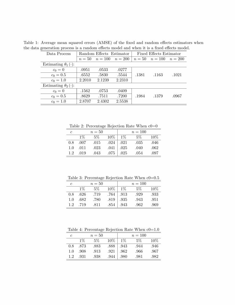
Table 1: Average mean squared errors (AMSE) of the �xed and random e�ects estimators whenthe data generation process is a random e�ects model and when it is a �xed e�ects model.

Data Process Random E�ects Estimator Fixed E�ects Estimatorn = 50 n = 100 n = 200 n = 50 n = 100 n = 200

Estimating �1 (�):c0 = 0 .0951 .0533 .0277c0 = 0:5 .6552 .5830 .5544 .1381 .1163 .1021c0 = 1:0 2.2010 2.1239 2.2310

Estimating �2 (�):c0 = 0 .1562 .0753 .0409c0 = 0:5 .8629 .7511 .7200 .1984 .1379 .0967c0 = 1:0 2.8707 2.4302 2.5538

Table 2: Percentage Rejection Rate When c0=0

c n = 50 n = 100

1% 5% 10% 1% 5% 10%

0.8 .007 .015 .024 .021 .035 .0461.0 .011 .023 .041 .025 .040 .0621.2 .019 .043 .075 .025 .054 .097

Table 3: Percentage Rejection Rate When c0=0.5

c n = 50 n = 100

1% 5% 10% 1% 5% 10%

0.8 .626 .719 .764 .913 .929 .9331.0 .682 .780 .819 .935 .943 .9511.2 .719 .811 .854 .943 .962 .969

Table 4: Percentage Rejection Rate When c0=1.0

c n = 50 n = 100

1% 5% 10% 1% 5% 10%

0.8 .873 .883 .888 .943 .944 .9461.0 .908 .913 .921 .962 .966 .9671.2 .931 .938 .944 .980 .981 .982