Nonparametric panel data models with interactive fixed effects∗

Joachim Freyberger‡

Department of Economics, University of Wisconsin - Madison

November 3, 2012

Abstract

This paper studies nonparametric panel data models with multidimensional, unobserved individual

effects when the number of time periods is fixed. I focus on models where the unobservables have

a factor structure and enter an unknown structural function nonadditively. A key distinguishing

feature of the setup is to allow for the various unobserved individual effects to impact outcomes dif-

ferently in different time periods. When individual effects represent unobserved ability, this means

that the returns to ability may change over time. Moreover, the models allow for heterogeneous

marginal effects of the covariates on the outcome. The first set of results in the paper provides

sufficient conditions for point identification when the outcomes are continuously distributed. These

results lead to identification of marginal and average effects. I provide further point identification

conditions for discrete outcomes and a dynamic model with lagged dependent variables as regres-

sors. Using the identification conditions, I present a nonparametric sieve maximum likelihood

estimator and study its large sample properties. In addition, I analyze flexible semiparametric and

parametric versions of the model and characterize the asymptotic distribution of these estimators.

Monte Carlo experiments demonstrate that the estimators perform well in finite samples. Finally,

in an empirical application, I use these estimators to investigate the relationship between teach-

ing practice and student achievement. The results differ considerably from those obtained with

commonly used panel data methods.

∗I am very grateful to my advisor Joel Horowitz as well as Ivan Canay and Elie Tamer for their excellent advice,constant support, and many helpful comments and discussions. I have also received valuable feedback from MattMasten, Konrad Menzel, Diane Schanzenbach, Arek Szydlowski, Alex Torgovitsky, and seminar particatipants atNorthwestern University. I thank Jan Bietenbeck for sharing his data. Financial support from the Robert EisnerMemorial Fellowship is gratefully acknowledged.‡Email: j.freyberger@u.northwestern.edu. Comments are very welcome.

1 Introduction

This paper is about identification and estimation of panel data models with multidimensional,

unobserved individual effects. In particular, I study models based on the outcome equation

(1) Yit = gt(Xit, λ

′iFt + Uit

), i = 1, . . . , n, t = 1, . . . , T,

where Xit ∈ Rdx is a random vector of explanatory variables, Yit is a scalar outcome variable,

and Uit is a scalar idiosyncratic disturbance term. The structural functions gt are unknown. Both

λi ∈ RR and Ft ∈ RR are unobserved vectors of unknown dimension R. I study models with both

continuously and discretely distributed outcomes. The explanatory variables Xit can be continuous

or discrete and may depend on the individual effects λi. In this paper, T is fixed while n→∞.

Nonlinear and nonparametric panel data models have recently received much attention.1 All of

these models are based on special cases of the general outcome equation

(2) Yit = gt (Xit, λi, Uit) , i = 1, . . . , n, t = 1, . . . , T,

where Uit and λi may be infinite dimensional. With Xi = (Xi1, . . . , XiT ) and x = (x1, . . . , xT ),

most of these models share the feature that

E [Yit | Xi = x, λi = λ1] < E [Yit | Xi = x, λi = λ2]

implies

E [Yis | Xi = x, λi = λ1] < E [Yis | Xi = x, λi = λ2] ,

for all s 6= t such that xs = xt. Consequently, the ranking of individuals with the same ob-

served characteristics, based on their expected outcome, cannot change over t without a change

in observables Xit. This condition usually follows because either it is assumed that λi is a

scalar and that E [Yit | Xi, λi] is strictly increasing in λi for all t, or because it is assumed that

E [Yit | Xi = x, λi = λ] = E [Yis | Xi = x, λi = λ] for s 6= t such that xs = xt. In contrast, models

based on (1) do not impose such assumptions, but instead allow for multidimensional unobserved

individual effects, which may affect the outcome variable Yit differently for different t. When in-

dividual effects represent unobserved abilities, this means that both the returns to the various

1I discuss the related literature in the next section.

1

abilities, as well as the relative importance of each ability on the outcome, can change over t.

Another important feature of model (1) is that it allows for heterogeneous marginal effects of the

covariates on the outcome, which implies, for example, that returns to education may depend on

unobserved ability.2

The flexibility of model (1) is important in many applications. For example, suppose that we

are interested in the relationship between teacher characteristics and student achievement. Assume

that each student i takes T tests, such as subject specific tests, and Yit is the outcome of test t for

student i. The vector Xit contains explanatory variables such as student, classroom, and teacher

characteristics. A linear fixed effects model, which is based on the outcome equation

Yit = X ′itβ + λi + Uit, i = 1, . . . , n, t = 1, . . . , T,

is often used in this setting. For example, Dee (2007) analyzes whether assignment to a same-gender

teacher has an influence on student achievement. Clotfelter, Ladd, and Vigdor (2010) and Lavy

(2011) investigate the relationship between teacher credentials and student achievement and teach-

ing practice and student achievement, respectively. In a linear fixed effects model λi is a scalar and

represents unobserved ability of student i. Loosely speaking, this model assumes that if student i

and j have the same observed characteristics and student i is better in subject t, say Mathematics,

then student i must also be better in subject s, say English. In contrast, the vector λi in model

(1) accounts for different dimensions of unobserved abilities and Ft represents the importance of

each ability for test t. Hence, the model allows some students to have abilities such that they have

a higher expected outcome in Mathematics, while others may have a higher expected outcome in

English, without changes in observables. Furthermore, the impact of a teacher on students may

differ for students with different abilities, which is ruled out in linear models. The main object of

interest in this setting could then be marginal effects of teacher characteristics on students’ test

outcomes for different levels of students’ abilities.

Other applications of model (1) include estimating returns to education or the effect of union

membership on wages. In these examples, t represents time and the outcome Yit is wage at time t

of person i. The covariates Xit may include years of education, experience, and union membership.

The vector λi represents different unobserved abilities of person i, and Ft represents the price of

these abilities at time t. Model (1) also applies to macroeconomic situations. For example, assume

2Equation (1) becomes a model when combined with assumptions in later sections. For simplicity I refer to theoutcome equation as model (1) in the introduction, because the structure is one of the models’ main features.

2

that Yit is output of country i in period t and Xit contains input variables such as labor and capi-

tal. The vector Ft denotes common shocks, such as technology shocks or a financial crisis, while λi

represents the heterogeneous impacts of the common shocks on country i.3

This paper presents sufficient conditions for point identification of model (1) when T is fixed

and n → ∞. All parameters of the model are point identified up to normalizations under the

assumptions in this paper. In models with this specific structure of the unobservables, the vec-

tor Ft is usually referred to as the factors, while λi are called the loadings. The factor structure

of the unobservables is commonly called interactive fixed effects because of the interaction of λi

and Ft. Since T is fixed and n → ∞, I treat Ft as a vector of constants and λi as a vector of

random variables.4 The identified parameters include the functions gt as well as the number of

factors R, the factors Ft, and the distributions of λi and Uit conditional on the observed covariates.

Although T is fixed, I require that T ≥ 2R + 1. This condition means that for a given T , only

factor models with less than or equal to T/2− 1 factors are point identified under the assumptions

I provide. These identification results imply identification of average effects as well as marginal

effects, which are often the primary objects of interest in applications. I first consider continuously

distributed outcomes, in which case the functions gt are assumed to be strictly increasing in the

second argument. The identification strategy follows two main steps. First, I use results from

the measurement error literature to show that the distribution of (Yi, λi) is identified up to some

nonunique features, such as any one to one transformation of λi. In the second step, I establish

uniqueness of all parameters by combining arguments from linear factor models and single index

models with unknown link functions. The set of assumptions provided in this case, rules out that

Xit contains lagged dependent variables and that the outcome Yit is discrete. Therefore, I discuss

several extensions to the above model where some assumptions are relaxed to accommodate these

cases. The cost is strengthening other assumptions. Most importantly, I require λi to be discretely

distributed if the outcomes are discrete, and T needs to be larger if Xit contains past outcomes.

After providing sufficient conditions for identification, I present a nonparametric sieve maxi-

mum likelihood estimator, which can be used to estimate the structural functions gt as well as the

factors and the conditional densities of λi and Uit consistently. The estimator requires estimat-

ing objects which might be high dimensional in applications, such as the conditional density of

λi. Therefore, in addition to a fully nonparametric estimator, this paper also provides a flexible

3For more examples in economics where factor models are applicable see Bai (2009) and references therein.4I use the terminology interactive fixed effects, although I make some assumptions about the distribution of λi.

Graham and Powell (2012) provide a discussion on the difference between fixed effects and correlated random effects.

3

semiparametric estimator. In this setup, I reduce the dimensionality of the estimation problem by

assuming a location and scale model for the conditional distributions. The structural functions can

be nonparametric, semiparametric, or parametric. In the latter two cases, many of the parameters

of interest are finite dimensional. I show that the estimators of the finite dimensional parameters

are√n consistent and asymptotically normally distributed, which yields confidence intervals for

these parameters. I also describe an easy to implement fully parametric estimator. Finally, I show

how the null hypothesis that the model has R factors can be tested against the alternative that the

model has more than R factors, and how this result can be used to consistently estimate the number

of factors. I provide Monte Carlo simulation results which demonstrate that the semiparametric

estimator performs well in finite samples.

In an empirical application, I use the semiparametric estimator to investigate the relationship

between teaching practice and student achievement. The outcome variables Yit are different math-

ematics and science test scores for each student i. The main regressors are a measure of traditional

teaching practice and a measure of modern teaching practice for each class a student attends. These

measures are constructed using students’ answers to questions about class activities. Traditional

teaching practice is associated with lecture based classes with an emphasis on memorizing defi-

nitions and formulas. Modern teaching practice is associated with cooperative group work and

justification of answers. The main objects of interest in this application are marginal effects of

teaching practice, on mathematics and science test scores, for different levels of students’ abilities.

Using a standard linear fixed effects model, I find a positive relationship between traditional teach-

ing practice and test outcomes in both mathematics and science. I then estimate model (1) with

two factors and obtain substantially different results. I still find a positive relationship between tra-

ditional teaching practice and mathematics test scores, but a positive relationship between modern

teaching practice and science test scores. Furthermore, the structural functions are significantly

nonlinear. In particular, the magnitude of the relationship between teaching practice and test out-

comes is higher for students with low abilities than for students with high abilities.

It should be noted that there are potential costs of identifying all features of model (1). In

particular, certain objects, such as average marginal effects, may be identified under weaker as-

sumptions. I leave these questions for future research and instead focus on point identification of

all parameters. This approach has the advantage that it leads to identification of many interesting

objects in applications, such as marginal effects for different levels of abilities.

The remainder of the paper is organized as follows. The next section connects this paper to

4

related literature on linear factor models, nonparametric panel data models, and measurement er-

ror models. Section 3 deals with identification of model (1) with continuous outcomes and without

lagged dependent variables as regressors. Section 4 extends the arguments to allow for lagged de-

pendent variables and discrete outcomes. Section 5 discusses different ways to estimate the model,

including the number of factors. Section 6 and 7 present Monte Carlo results and the empirical

application, respectively. Finally, Section 8 concludes. All proofs are contained in the appendix.

2 Related literature

This paper is related to a vast literature on linear factor models, nonlinear and nonparametric

panel data models, and measurement error models. Linear factor models are well understood and

provide a way to deal with multidimensional unobserved heterogeneity. The model usually is

Yit = X ′itβ + λ′iFt + Uit, i = 1, . . . , n, t = 1, . . . , T.

The theoretical econometrics literature on linear factor models includes Holtz-Eakin, Newey, and

Rosen (1988), Ahn, Lee, and Schmidt (2001), Bai and Ng (2002), Bai (2003), Andrews (2005),

Pesaran (2006), Bonhomme and Robin (2008), Bai (2009), Ahn, Lee, and Schmidt (2010), Moon

and Weidner (2010), Bai and Ng (2011), and Bai (2012). Some papers (e.g. Bai 2009) let n→∞

and T → ∞ while others (e.g. Ahn et al. 2010) have T fixed and n → ∞, as in this paper.

Estimating the number of factors is considered by Bai and Ng (2002). Nonlinear additive factor

models of the form

Yit = g (Xit) + λ′iFt + Uit, i = 1, . . . , n, t = 1, . . . , T

have been studied recently by Huang (2010) and Su and Jin (2012), in a setup where n → ∞

and T → ∞. The drawback of linear models is that they impose homogeneous marginal effects.

In my application this means that the influence of teachers on students is identical for students

with different abilities. Moreover, the analysis in these papers is tailored to the linear model. For

example, Bai (2009) estimates the factors using the method of principal components.

Factor models have been used in several applications. Related to the application in this paper,

Carneiro, Hansen, and Heckman (2003) use five test scores to estimate a linear factor model with

two factors. Heckman, Stixrud, and Urzua (2006) use a linear factor model to explain labor mar-

5

ket and behavioral outcomes. Cunha and Heckman (2008) and Cunha, Heckman, and Schennach

(2010) estimate the evolution of cognitive and noncognitive skills with factor models. Williams,

Heckman, and Schennach (2010) study a model where the first stage is a linear factor model and

the estimated factor scores are used in a nonparametric second stage. They use their model to

estimate the technology of skill formation.

Many recent papers in the nonparametric panel data literature with continuously distributed

outcomes are related to the model I consider.5 Evdokimov (2010, 2011) provides identification

results for nonlinear models with a scalar heterogeneity term. Arellano and Bonhomme (2012)

analyze a random coefficients model which allows for multidimensional unobserved heterogeneity.

Other nonnested setups include Chernozhukov, Fernandez-Val, Hahn, and Newey (2012), Graham

and Powell (2012), and Hoderlein and White (2012) who mainly focus on identification and estima-

tion of average marginal effects and quantile effects. In all these papers, the ranking of individuals

based on their mean or median outcome cannot change over t without changes in observable regres-

sors. Bester and Hansen (2009) are also concerned with average marginal effects but do not impose

this assumption. Instead they restrict the conditional distribution of λi. Altonji and Matzkin

(2005) require an external variable which they construct in a panel data model by restricting the

conditional distribution of λi.

Nonlinear panel data models with discrete outcomes generally need a different treatment. For

example Chamberlain (2010) shows that in binary outcome panel data models, point identification

fails in case the support of the regressors is bounded and the disturbance is not logistic distributed.

Honore and Tamer (2006) demonstrate lack of point identification in a similar model with lagged

dependent variables. Williams (2011) derives partial identification results for panel data models

with discrete outcomes and shows that the identified set converges to a point as T →∞. The iden-

tification strategy used in my paper yields point identification of the distribution of (Yi, λi) | Xi

with discrete outcomes, provided that λi has a discrete distribution as well.

The identification strategy with continuously distributed outcomes is related to Hu and Schen-

nach (2008) and Cunha, Heckman, and Schennach (2010), because it relies on an eigendecomposi-

tion of a linear operator, but the arguments differ in important steps. Hu and Schennach (2008)

study a nonparametric measurement error model with instrumental variables. The connection

to the factor model is that λi can be seen as unobserved regressors. A subset of the outcomes

represents the observed and mismeasured regressors, while another subset of outcomes serves as

5Arellano and Bonhomme (2011) provide a recent survey on nonlinear panel data models.

6

instruments. Cunha, Heckman, and Schennach (2010) apply results in Hu and Schennach (2008) to

identify a nonparametric factor model similar to model (2). One of their identifying assumptions

fixes a measure of location of the distribution of a subset of outcomes given λi.6 Such measures

generally do not exist in model (1) when all functions gt are unknown. Instead, I use the relation

between Yit and λi delivered by (1), combined with arguments from linear factor models and single

index models with unknown link functions. Hence, the two models are nonnested. Furthermore, the

different sets of outcomes, which represent regressors and instruments, are interchangeable which

allows me to show that T = 2R+ 1 is sufficient for identification in model (1). The structure of the

model also leads to more primitive sufficient conditions for some of the high level assumptions.7

Similarly, in the case of discrete λi, the identification strategy is related to the one of Hu (2008)

who is concerned with a measurement error model with one discrete mismeasured regressor. The

identification strategy with lagged dependent variables is related to Hu and Shum (2012) and Sasaki

(2012) who use arguments related to the approach of Hu and Schennach (2008). Again, I do not

impose one of their main identifying assumptions, but instead use the additional structure of the

factor model. Shiu and Hu (2011) study a dynamic panel data model with covariates which requires

certain conditions on the process of Xit. The assumptions in all these papers are nonnested with

the assumptions I present. I complement these papers by focusing on the factor structure of the

error terms but by using different conditions which allow for different interesting models.

3 Identification of static factor model with continuous outcomes

This section is about identification of a model based on (1) with continuously distributed outcome

variables Yit and continuously distributed λi. I first introduce important notation and state the

assumptions. Afterwards, I discuss the assumptions and show that they are sufficient for identifi-

cation. To simplify the notation, I first assume that the number of factors R is known. In Section

3.3 I show how the number of factors can be identified.

3.1 Assumptions, definitions, and notation

As stated in the introduction, I assume in this section that the structural functions gt are strictly

increasing in the second argument. Define the inverse function ht (Yit, Xit) ≡ g−1t (Yit, Xit). Then

6The corresponding assumption in Hu and Schennach (2008) fixes a measure of location of the distribution of themeasurement error.

7These assumptions are invertibility of integral operators. Lemma 1 provides sufficient conditions.

7

equation (1) can be written as

(3) ht (Yit, Xit) = λ′iFt + Uit, i = 1, . . . , n, t = 1, . . . , T.

A necessary condition for point identification is T ≥ 2R+1.8 To simplify the notation I assume

that T = 2R+ 1, but the extension to a larger T is straightforward. In fact, the assumptions with

a larger T are weaker, as discussed below.

Assumption S1. R is known and T = 2R+ 1.

I now introduce some important definitions and notation followed by the remaining assumptions.

For each t, let Xt ⊆ RK and Yt ⊆ R be the supports of Xit and Yit, respectively. Let Λ ⊆ RR be the

support of λi. Define Xi = (Xi1, . . . , XiT ) and define Yi and Ui analogously. Let X ≡ ∪Tt=1Xt and

Y ≡ ∪Tt=1Yt be the supports of Xi and Yi, respectively. Define the vector of the last R outcomes

Zi1 ≡(Yi(R+2), . . . , Yi(2R+1)

).

Let K ≡ {k1, k2, . . . , kR} ⊂ {1, 2, . . . , R + 1} be a set of any R integers between 1 and R + 1 with

k1 < k2 < . . . < kR. Let kR+1 ≡ {1, 2, . . . , R+ 1} \K be the remaining integer. Define

ZiK ≡ (Yik1 , . . . , YikR) and

ZikR+1≡ YikR+1

.

For example, if R = 2 and T = 5, then Zi1 = (Yi4, Yi5) and ZiK can be (Yi1, Yi2) or (Yi1, Yi3) or

(Yi2, Yi3). The scalar ZikR+1is the remaining outcome which is neither contained in Zi1 nor in ZiK .

Let Z1 ⊆ RR and ZK ⊆ RR be the supports of Zi1 and ZiK , respectively.

The conditional probability mass or density function of any random variable W | V is denoted

by fW |V (w; v) and the marginal probability density (or mass) function by fW (w). Let FW |V (w; v)

and FW (w) be the cumulative distribution functions of W | V and W , respectively. The α-quantile

of W | V is denoted by Qα[W | V ]. The median, Q1/2[W | V ], is denoted by M [W | V ]. A random

variable W is complete for V if for all real measurable functions m such that E[|m(W )|] <∞

E[m(W ) | V ] = 0 a.s. implies that m (W ) = 0 a.s.

8This is shown by Carneiro, Hansen, and Heckman (2003) in a linear factor model with covariance restrictions.Related arguments can be used here to establish that point identification fails if T < 2R+ 1.

8

W is bounded complete for V if the implication holds for any bounded function m.

Let F be the R× T matrix containing all factors and write it as

(4) F =(F1 F2 · · · FT

)=(F 1 F 2 F 3

)where F 1 is R×R, F 2 is R× 1, and F 3 is R×R. Let IR×R denote the R×R identity matrix.

This section focuses on the continuous case. Therefore, I make the following assumption.

Assumption S2. fYi1,...,YiT ,λi|Xi (y1, . . . , yT , λ;x) is bounded on Y1×· · ·×YT×Λ×X and continuous

in (y1, . . . , yT , λ) ∈ Y1 × · · · × YT × Λ for all x ∈ X . All marginal and conditional densities are

bounded.

Next, I present several additional assumptions. In addition to assuming that ht is strictly

increasing in the first argument, I require location and scale normalizations. Second, I use moment

restrictions, independence assumptions, and completeness conditions. Finally, just as in linear

factor models, the factors and loadings are only identified up to a transformation.

Assumption S3.

(i) ht is strictly increasing and differentiable in its first argument.

(ii) Let yt = M [Yit]. There exist xt ∈ Xt such that ht(yt, xt) = 0 for all t = R + 2, . . . , 2R + 1

and ∂ht(yt,xt)∂y = 1 for all t = 1, . . . , T.

Assumption S4. M [Uit | Xi, λi] = 0 for all t = 1, . . . , T . If R = 1, Qα [Uit | Xi, λi] is independent

of λi for all α in a neighborhood of 1/2.

Assumption S5. Ui1, . . . , UiT are jointly independent conditional on λi and Xi.

Assumption S6. F 3 = IR×R and F 1 has full rank.

Assumption S7. The R×R covariance matrix of λi has full rank conditional on Xi.

Assumption S8. Zi1 is bounded complete for ZiK for any R integers K ⊂ {1, . . . , R + 1} condi-

tional on Xi. Moreover, λi is bounded complete for Zi1 conditional on Xi.

The location normalizations in Assumption S3 are needed because without them one could

add a constant c to λir as well as cFtr to ht without affecting equality (3). The location of Uit

is fixed by Assumption S4. Similarly, the scale normalizations are needed because otherwise for

9

t = T − R + 1, . . . , T one can multiply ht, λi and Uit by a constant c while for all other t one can

multiply ht, Ft and Uit by c. The assumption that the standardizations occur at the median of Yit

is only used for a minor part of the main identification theorem as discussed below.

Assumption S4 implies that while the regressors can arbitrarily depend on λi, they are strictly

exogenous with respect to Uit. This assumption rules out, for example, that Xit contains lagged

dependent variables. Moreover, for R = 1, the model would not be identified without the second

part of Assumption S4. To see this, let B(λ) be any strictly increasing function and let Ft = 1 for

all t. Then

Yit = gt

(Xit, B

−1(λi + Uit

))where λi = B(λi) and Uit = B (Uit + λi) − B(λi) and Uit satisfies the median restriction. As-

sumption S5 is strong but independence is hard to avoid in nonadditive models. Although the

unobservables λ′iFt + Uit are correlated over t, the assumption says that any dependence is due

to λi. Autoregressive Uit are thus ruled out. However, note that the assumptions do not require

that Uit and Xit are independent, nor that Uit and λi are independent. Hence, heteroskedasticity

is permitted.

Assumption S6 is a normalization which is needed because for any R×R invertible matrix H

λ′iFt = λ′iHH−1Ft = (H ′λi)

′(H−1Ft) = λ′iFt.

Although the linear combination λ′iFt can be identified, the factors and loadings can only identified

up to a transformation since λ′iFt = λ′iFt. Hence R2 restrictions on the factors and loadings are

needed to identify a certain transformation, which I impose by assuming that F 3 = IR×R. This

normalization corresponds to H = F 3 above and implicitly assumes that F 3 is invertible.9

Assumption S7 is a rank condition which rules out that some element of λi is a linear combination

of the other elements. Furthermore, all constant elements of λi, and thus time trends, are absorbed

by the function ht.

Assumption S8 is a bounded completeness condition. Completeness conditions are often used in

nonparametric instrumental variable models, in which case the regressor is required to be complete

for the instrument. This condition is a generalization of the rank condition in linear instrumental

variable regressions. The first part of Assumption S8 therefore says that ZiK serves as an instrument

9In linear factor models it is often assumed that the factors are orthogonal and have length 1 and that thecovariance matrix of the loadings is diagonal. This is convenient in the linear model because, when estimating thefactors by the method of principal components, the estimates are orthogonal.

10

for Zi1. The second part ensures that λi does not contain too much information relative to Zi1

which, for example, rules out that λi is continuously distributed while Zi1 is discrete. In some

models this assumption can be hard to interpret.10 However, here since gt is strictly increasing,

Assumption S8 is solely an assumption about the distribution of λi and Uit given Xi and the values

of Ft. The next lemma provides lower level sufficient conditions for this assumption to be satisfied.

Lemma 1. Assume that any R × R submatrix of F has full rank and that λi has support on RR

conditional on Xi. Moreover, assume that the characteristic function of Uit is nonvanishing on

(−∞,∞) for all t, and that Ui ⊥⊥ λi . Then Assumptions S3(i) and S5 imply Assumption S8.

A nonvanishing characteristic function holds for many standard distributions such as the normal

family, the t-distribution, or the gamma distribution. However, it does not hold for all distributions,

for instance uniform and triangular distributions. As an important special case, the lemma shows

that if λi and Ui are normally distributed and independent, and the covariance matrix of λi as well

as any R×R submatrix of F have full rank, then Assumption S8 holds.

If T > 2R + 1, then Assumption S8 only needs to hold for R + 1 different sets of R integers

K = {k1, k2, . . . , kR}. Also only for one these sets the full rank part of Assumption S6 has to hold.

3.2 Identification of gt and Ft and the conditional distributions of λi and Uit

In this section I outline the main arguments for identifying gt, the factors, as well as the distribution

of (Ui, λi) | Xi. Afterwards, I state the main identification theorem. The formal proof is given in

the appendix. In the next subsection I prove identification of the number of factors.

To use the scale and location normalizations define

X ≡ {(x1, . . . , xT ) ∈ X : xt = xt for all t = R+ 2, . . . , 2R+ 1} .

where xt is defined in Assumption S3. The role of this set is explained below. In the appendix, it

is shown that Assumption S5 implies an operator equivalence result of the form

L1,kR+1,K = L1,λDkR+1,λLλ,K ,

where L1,kR+1,K , L1,λ, and Lλ,K are linear integral operators and DkR+1,λ can be seen as a diagonal

operator. The operator on the left hand side only depends on the population distribution of the

10Canay, Santos, and Shaikh (2012) show that the assumption is not testable under commonly used restrictions.

11

observables, while all operators on the right hand side depend on the joint distribution of Yi and

λi. Assumption S5 also yields a second operator equivalence result

L1,K = L1,λLλ,K .

The operator on the left hand side again depends on the population distribution of the observables

only. Assumption S8 implies that the inverse of L1,λ exists and can be applied from the left.

Therefore

L−11,λL1,K = Lλ,K

and in turn

L1,kR+1,K = L1,λDkR+1,λL−11,λL1,K .

Assumption S8 also ensures that the right inverse of L1,K exists which means that

(5) L1,kR+1,KL−11,K = L1,λDkR+1,λL

−11,λ.

In a paper on measurement error models, Hu and Schennach (2008) obtain a similar operator

equality. They show that the right hand side is an eigenvalue-eigenfunction decomposition of the

operator on the left hand side and that such a decomposition is unique up to three nonunique

features. It is shown in the appendix that, conditional on Xi ∈ X , these nonunique features cannot

arise in model (1) under the assumptions provided in Section 3.1. To do so, I combine arguments

from linear factor models and single index models with unknown link functions. The most important

assumptions which are used to establish uniqueness are the factor structure, the normalizations,

the moments conditions, and monotonicity of the structural functions. Furthermore, I use that

the outcomes contained in ZiK are interchangeable, which ensures that T = 2R + 1 is sufficient

for identification. The left hand side of the operator equality (5) only depends on the population

distribution of the observables. Uniqueness of the decomposition thus ensures that the operators

L1,λ and DkR+1,λ are identified. It can then be shown that Lλ,K is also identified. Identification of

these integral operators is in this case equivalent to identification of fYi,λi|Xi . It then follows that

Ft is identified. Finally, under additional assumptions, it is shown that gt and the distribution of

Ui, λi | Xi are identified.

The previous arguments lead to the following theorem which is one of the main results in this

paper. The formal proof is given in the appendix.

12

Theorem 1. Assume that Assumptions S1 - S8 hold. Then fYi,λi|Xi(s, λ;x) is identified for all

s ∈ Y, λ ∈ Λ, and x ∈ X . Moreover, Ft is identified. Assume in addition that either λi has support

on RR or that Ui ⊥⊥ λi. Then the functions gt as well as the distribution of (Ui, λi) | Xi = x are

identified for all x ∈ X .

Remark 1. Without the additional assumption that either λi has support on RR or that Ui ⊥⊥ λi,

the functions gt and ht are identified on a subset of the support of λ′iFt + Uit and the support of

Yit, respectively. For example, gt(xt, et) is identified for all et such that et = λ′Ft for some λ ∈ Λ.

The normalization at the median of Yit in Assumption S3 is only used to identify Ft in cases where

gt is not identified for all values on the support.

Theorem 1 shows identification for all x ∈ X which is a strict subset of the support of Xi. After

identifying the structural functions and distributions for all x ∈ X , these quantities can be shown

to be identified for x /∈ X . To do so for any (x1, . . . , xT ) ∈ X take (xR+1, . . . , x2R+1) such that

fXi(R+1),...,Xi(2R+2)|Xi1,...,XiR (xR+1, . . . , x2R+1; x1, . . . , xR) > 0.

Since ht(yt, xt) is identified for all t = 1, . . . , R, in the proof of the theorem the roles of the

different periods t can be switched. In particular, instead of using a normalization at xt for t =

R + 2, . . . , 2R + 1, the values xt for t = 1, . . . , R can take this role. It follows that for these

(xR+1, . . . , x2R+1), the function ht is identified. This process can be iterated.

Hence, in the most favorable case, if fXi (x) > 0 for all x ∈ X1 × · · · × XT , the functions ht are

identified for all xt ∈ Xt. On the other hand, if Xit = xi or Xit = xt for all i and t, ht is only

identified at xt for all t. This is a standard problem in panel data models. If the regressor does

not change over t, it is not possible to distinguish between the effect of Xit and the effect of λi

on the outcome, without restricting the dependence between Xit and λi. Moreover, the function

ht depends on t. Thus, if Xit = xt, a change in Xit cannot be distinguished from a change in

the function. A similar problem occurs with time fixed effects in linear panel data models. There

are many intermediate cases where ht is identified for all xt ∈ Xt. This is, for example, the

case my empirical application (see Section 7.3 for the details), where neither fXi (x) > 0 for all

x ∈ X1 × · · · × XT nor Xit = xi or Xit = xt for all i and t. Finally, if the structural functions

are parametric, which is likely to be assumed in applications, it is easier to identify the model.

For instance, if ht is linear in a scalar Xit, identification at two points implies identification for all

xt ∈ Xt.

13

3.3 Identification of the number of factors

To identify the number of factors let R ∈{

1, . . . ,⌊T2

⌋}, where

⌊T2

⌋is the largest integer smaller

than or equal to T2 , and define

Zi1 ≡(Yi(T−R+1), . . . , YiT

)and Zi2 ≡

(Yi1, . . . , YiR

).

It can be shown that under the previous assumptions and λi ⊥⊥ Ui, Zi1 is bounded complete for Zi2

only if R ≤ R. Hence, R is the largest integer R, less than or equal to T2 , such that Zi1 is bounded

complete for Zi2. Since this condition only involves the data, it implies the following theorem.

Theorem 2. Assume that Assumptions S2, S3, S5, and S8 hold, that λi ⊥⊥ Ui, and that T ≥ 2R+1.

Then the number of factors, R, is identified.

Remark 2. More lengthy arguments than those in the proof of Theorem 2 can be used to show that

the number of factors is identified without the completeness assumption. This result is important

for estimating the number of factors, because there are no known conditions under which the

completeness assumption is testable as shown by Canay, Santos, and Shaikh (2012).

3.4 Functionals invariant to normalizations

Although a few normalization assumptions are needed in Theorem 1, many potential objects of

interest are invariant to these normalizations. Define Cit ≡ λ′iFt. Next let Qα[Cit | Xi = x] and

Qα[Uit | Xi = x] be the conditional α-quantile of Cit and Uit, respectively. Fix any t and let xt ∈ Xt

as well as x ∈ X such that the previous identification results hold. Appendix A.4 shows that the

following functionals are invariant to the normalizations in this paper.

1. Function values at quantiles of unobservables:

gt (xt, Qα1 [Cit | Xi = x] +Qα2 [Uit | Xi = x])

or

gt (xt, Qα [Cit + Uit | Xi = x]) .

2. Average function values: ∫gt (xt, e) dFCit+Uit|Xi=x (e)

14

or ∫gt (xt, e+Qα [Uit | Xi]) dFCit|Xi=x (e) .

It then immediately follows that also differences of function values or differences of average function

values are invariant to these normalizations. These quantities can be used to answer important

policy questions. For example one could answer questions about the effect of a change in class size

on test outcomes for students with different levels of abilities.

4 Further identification results

Assumptions S4 and S5 rule out that Xit contains lagged dependent variables. In this section I

relax these assumptions to accommodate this case. To do so, I must strengthen other assumptions.

Furthermore, I discuss the case of discretely distributed heterogeneity, in which case Yit may also

be discretely distributed.

4.1 Dynamic factor model with continuous outcomes

First rewrite equation (1) to

(6) Yit = gt(Yi(t−1), Xit, λ

′iFt + Uit

), i = 1, . . . , n, t = 1, . . . , T.

I assume for simplicity that R is known and that there is only one lagged dependent variable.

Several lagged dependent variables can be incorporated using similar arguments to the ones pre-

sented below. The main difference to the static model is that in the static case, periods t were

interchangeable, which is not the case with lagged dependent variables. Therefore, T needs to be

larger for the model to be identified.

Using lagged dependent variables requires adapting the arguments of Section 3. As explained

in Section 2, similar arguments, in models nonnested with the one considered here, have been used

by Shiu and Hu (2011), Hu and Shum (2012), and Sasaki (2012). I assume for simplicity that

there are no (strictly exogenous) regressors Xit. Using these regressors simply requires to make all

assumptions conditional on Xi just as in Section 3. Hence, the outcome equation is

Yit = gt(Yi(t−1), λ

′iFt + Uit

), i = 1, . . . , n, t = 1, . . . , T, or

ht(Yit, Yi(t−1)

)= λ′iFt + Uit, i = 1, . . . , n, t = 1, . . . , T.

15

The identification strategy requires that T ≥ 2R+⌈R2

⌉+ 3 where dAe is the smallest integer larger

than or equal to A. To simplify the exposition, I assume that T = 3R + 3. In the appendix it is

explained how the model can be identified, under modified assumptions, with smaller T . In this

section let K = {k1, k2, . . . , kR} be R integers between 2R+ 3 and 3R+ 3 with k1 < k2 < . . . < kR.

Also define ZiK ≡ (Yik1 , . . . , YikR) and Zi1 ≡ (Yi1, . . . , YiR). Notice that the definitions of Zi1 and

ZiK are slightly different to the ones used in Section 3. As before, IR×R is the R × R identity

matrix and F 3 is the matrix of factors from the last R periods.

Assumption L1. R is known and T = 3R+ 3.

Assumption L2. fYi1,...,YiT ,λi (y1, . . . , yT , λ) is bounded on Y1 × · · · × YT × Λ and continuous in

(y1, . . . , yT , λ) ∈ Y1 × · · · × YT × Λ. All marginal and conditional densities are bounded.

Assumption L3.

(i) ht is strictly increasing and differentiable in its first argument.

(ii) Let yt = M [Yit]. For all t = 2R + 4, . . . , 3R + 3 it holds that ht(yt, yt−1) = 0 and for all

t = 1, . . . , T it holds that ∂ht(yt,yt−1)∂y = 1.

Assumption L4. M[Uit | Yi1, . . . , Yi(t−1), λ

]= 0 for all t = 2, . . . , T . If R = 1, for all α in a

neighborhood of 1/2, Qα[Uit | Yi1, . . . , Yi(t−1), λi

]is independent of λi.

Assumption L5. For all t ≥ 2, (UiT , . . . , Uit) ⊥⊥ (Yi(t−1), . . . , Yi1) | λi.

Assumption L6. For any R integers K ⊂ {2R+ 3, 2R+ 4, . . . , 3R+ 3}, ZiK is bounded complete

for Zi1 given Yi(R+1) and Yi(2R+2). Moreover, λi is bounded complete for ZiK given Yi(2R+2). If

R = 1, Yi6 is bounded complete for Yi1 given Yi(R+1), Yi(2R+2) and Yi(2R+3).

Assumption L7. For all λ1 6= λ2 and for all s2R+2, there exist s2R+1, . . . , sR+1 such that

fYi(2R+1),...,Yi(R+2)|Yi(2R+2),Yi(R+1),λi(s2R+1, . . . , sR+2; s2R+2, sR+1, λ1)

6= fYi(2R+1),...,Yi(R+2)|Yi(2R+2),Yi(R+1),λi(s2R+1, . . . , sR+2; s2R+2, sR+1, λ2).

Assumption L8. F 3 = IR×R.

Assumption L9. The R×R covariance matrix of λi has full rank conditional on Yi1, . . . , YiT .

16

The intuition for the certain number T required is that different sets of past outcomes serve

as instruments for future outcomes. However, the sets are limited due to the dynamic structure.

Hence, T needs to be larger compared to the static case. Assumption L3 is the same normalizing

assumption made in the static case. Assumption L4 is a location normalization for Uit. It also says

that the median of future values of Uit are median independent of λi and past values of Yit. Again,

an additional restriction for R = 1 is needed. Assumption L5 relaxes the previous assumption that

Uit and Uis are independent given all regressors Xi. Assumption L6 is a completeness assumption

similar as before: Past outcomes need to serve as instruments for future outcomes and λi cannot

have too much variation relative to Yit. By Assumption L5, the dependence between ZiK and Zi1

can only come through λi. Hence, I implicitly make an assumption about the joint distribution

of λi, Yi1, . . . , YiR. If, for example, λi ⊥⊥ (Yi1, . . . , YiR), this assumption fails. Assumption L7 is

similar. It says that given Yi(2R+2), λi still affects Yi(2R+1), . . . , Yi(R+2) for some Yi(R+1). This

assumption fails, for example, if λi ⊥⊥ (Yi(2R+1), . . . , Yi(R+2)) | (Yi(2R+2), Yi(R+1)) but is not strong

in general since Yi(2R+1), . . . , Yi(R+2) is of the same dimension as λi. It is mainly rules out that λi is

a deterministic function of Yit for some t. The last three assumptions together say that Yit has to

be affected by λi but cannot be explained perfectly by it. Appendix B.2 explains these assumptions

in more detail using a particular example. The main result of this section now follows.

Theorem 3. Let Assumptions L1 - L9 hold. Then fYi,λi(s, λ) is identified for all s ∈ Y and λ ∈ Λ.

Moreover, Ft is identified for all t ≥ 2. Assume in addition that either λi has support on RR or

that Ui ⊥⊥ λi. Then for all t ≥ 2 the functions gt as well as the distribution of (Ui2, . . . , UiT , λi) are

identified.

The conclusions are similar to the static case. The main difference is that F1, g1 and the

distribution of Ui1 are not identified because Yi0 is not observed.

4.2 Factor models with discrete heterogeneity

Above I assumed that Yi and λi are continuously distributed. If λi is continuously distributed

and Yi is discrete, then the distribution of (Yi, λi) | Xi is in general not nonparametrically point

identified. This is shown by Honore and Tamer (2006) and Chamberlain (2010) in dynamic and

static binary choice models, respectively. In this section, I focus on nonparametric identification

of the distribution of (Yi, λi) | Xi when λi is discrete and Yit is either discrete or continuous. I

examine the static case, but the dynamic case can be analyzed analogously using arguments from

17

Section 4.1.

Many of the assumptions below are similar to the ones in Section 3. However, some of the

previous assumptions are too strong when λi is discretely distributed. One reason is that the

completeness assumption (Assumption S8) implies that Yit and λi have the same number of points

of support, which is stronger than needed. The assumptions below can be satisfied if the number

of points of support of λi is less than or equal to the number of points of support of Yit. This

distinction could be interesting in applications when, for example, Yit is continuously distributed

but one only wants to allow for a high type and a low type and thus, λi is binary.

Let supp(λir) = {λ1r , . . . , λ

Sr } be the support of the rth element of λi. Assume that S, the

number of points of support, is known and is the same for all r = 1, . . . , R. Let supp(Yit) be the

support of Yit and let |supp(Yit)| be the number of points of support, which could be infinity. Again

(7) Yit = gt(Xit, λ

′iFt + Uit

), i = 1, . . . , n, t = 1, . . . , T.

The points of support of λi do not have to be known. The results in this section show identification

of the distribution of (Yi, λi) | Xi where λir ∈ {λ1r , . . . , λ

Sr }, which implies identification of marginal

effects for different quantiles of λi. The assumptions are as follows.

Assumption D1. R is known and T = 2R+ 1.

Assumption D2. Ui1, . . . , UiT are jointly independent conditional on λi and Xi.

Assumption D3. S < ∞ is known. Moreover, supp(λi) = supp(λi1) × · · · × supp(λiR). Assume

that Yit has the same number of points of support for each t, and S ≤ |supp(Yit)|.

Let A1, . . . , AS be a partition of the support of Yit such that for all as1 ∈ As1 and as2 ∈ As2

with s1 < s2 it holds that as1 < as2 . Define Zi1, ZiK , and ZikR+1as in Section 3.1. Let M =

R × S. Let C1, . . . , CM be a partition of the support of ZiK (and thus also of Zi1) such that

Cm = Am1 × · · · × AmR . For example if Yit ∈ {0, 1} and S = 2, then A1 = {0} and A2 = {1} as

well as C1 = {0, 0}, C2 = {0, 1}, C3 = {1, 0}, and C4 = {1, 1}.

Conditional on Xi and for all mK ,m1 ∈ {1, . . . ,M} define

PmK ,m1 ≡ P (ZiK ∈ CmK , Zi1 ∈ Cm1) .

Let L1,K be the M ×M matrix containing the probabilities such that mK increases over rows while

18

m1 increases over columns. That is

L1,K ≡

P1,1 P1,2 · · · P1,M

P2,1 P2,2 · · · P2,M

......

. . ....

PM,1 PM,2 · · · PM,M

.

Let λ1, . . . , λM be an ordering of all points of support of λi. Let L1,λ be the M × M matrix

containing

Pl,m1 = P(Zi1 ∈ Cm1 | λi = λl

)with l increasing over rows and m1 increasing over columns.

Assumption D4. L1,K is invertible for any ordering K conditional on Xi. L1,λ is invertible

conditional on Xi.

Assumption D5. P (Yit ∈ AS | λi) is strictly increasing in λ′iFt.

Assumption D6. F 3 = IR×R and F 1 has full rank, where F 1 and F 3 are defined in equation (4).

The assumptions are similar to the ones in the continuous case. The assumption that Yit has

the same support for all t is not needed but used to simplify the notation. Invertibility of the

matrix L1,K is analogous to a completeness assumption and is similar to identification conditions

in nonparametric instrumental variable models with discrete instruments and discrete regressors.

Invertibility of L1,λ implies that λi has at most as many points of support as Zi1. While for R = 1,

Assumption D6 is just a normalization, it is important to notice that F 3 = IR×R is not just a

normalization if R > 1. The reason is that for all t, λ′iFt has up to R2 points of support while

λi only has R points of support. The assumption is used for the ordering of the eigenvectors in

the eigendecomposition. It can easily be replaced by different assumptions in specific models as

illustrated in Section C.2. These assumptions lead to the following theorem.

Theorem 4. Assume that Assumptions D1 - D6 hold. Then, conditional on Xi ∈ X ,

P (Yi1 ∈ B1, . . . , YT ∈ BT , λi = λm)

is identified for all Bt ⊆ Yt for all t = 1, . . . , T and m ∈ {1, . . . ,M}.

19

5 Estimation

In this section, I describe how the static factor model with continuous outcomes and continuous

heterogeneity can be estimated. I first discuss estimation of the structural functions and the

distribution of (Ui, λi) ⊥⊥ Xi for a known number of factors. There are many papers with similar

estimation problems. Most closely related are the papers by Ai and Chen (2003), Hu and Schennach

(2008), and Carroll, Chen, and Hu (2010). In Section 5.2 I show how the null hypothesis that the

model has R factors can be tested against the alternative that the model has more than R factors,

and how this result can be used to consistently estimate the number of factors.

5.1 Estimation with a known number of factors

First notice that by Assumptions S3 and S5, the density of Yi given Xi can be written as

fYi1,...,YiT |Xi(y;x) =

∫ T∏t=1

fUit|Xi,λi(ht (yt, xt)− λ′Ft;x, λ)h′t (yt, xt) fλi|Xi(λ;x)dλ,

where h′t (yt, xt) denotes the derivative with respect to the first argument. Section 3 establishes that

there are unique functions fUit|Xi,λi , ht, and fλi|Xi as well as vectors Ft such that the conditional

density can be written in this way. Due to this uniqueness result, estimation can be based on the

sieve maximum likelihood method. The idea of sieve estimators is that the unknown functions are

replaced by a finite dimensional approximation, which becomes more accurate as the sample size

increases.11 Although I show that a completely nonparametric maximum likelihood estimator is

consistent, such an estimator is likely to be unattractive in applications due to the high dimension-

ality of the estimation problem. For example, the unknown function fλi|Xi(λ;x) is a function of

R+Tdx arguments where dx denotes the dimension of Xit. Furthermore, the nonparametric rates of

convergence in the strong norm (introduced below) can be very slow because the model nests non-

parametric deconvolution problems of densities which can have a logarithmic rate of convergence.12

Therefore, in practice a more convenient approach is a semiparametric estimator. The semipara-

metric estimator discussed in this paper reduces the dimensionality of the estimation problem by

assuming a location and scale model for the conditional distributions. The structural functions

can be nonparametric, semiparametric, or parametric. In the latter two cases, many parameters of

interest are finite dimensional. I show that these estimated finite dimensional parameters are√n

11For an overview of sieve estimators see Chen (2007).12For related setups see for example Fan (1991), Delaigle, Hall, and Meister (2008), and Evdokimov (2010).

20

consistent and asymptotically normally distributed.

In the following subsections, I present three kinds of estimators. First, I discuss consistency

of a fully nonparametric sieve estimator. Next, I present the semiparametric estimator. Finally, I

describe a fully parametric estimator and its asymptotic distribution.

5.1.1 Fully nonparametric estimator

I prove nonparametric consistency in a very general setup. All assumptions are listed in the

appendix. In this section I outline the main assumptions and discuss how the estimator can be

implemented. I first impose smoothness restrictions on the unknown functions. To do so, for any

d-dimensional multi-index a define |a| ≡∑d

j=1 aj . For any z ∈ Z ⊆ Rd denote the |a|-th derivative

of a function η : Rd → R by

∇aη(z) =∂|a|

∂za11 · · · ∂zadd

η(z),

where ∇aη(z) = η(z) if aj = 0 for all j = 1, . . . , d. For any γ > 0, let γ be the largest integer strictly

smaller than γ. Denote by Λγ(Z) the Holder space with smoothness γ. These are all functions such

that the first γ derivatives are bounded and the γ-th derivative is Holder continuous with exponent

γ − γ. That is, for all η ∈ Λγ(Z) it holds that

max|a|≤γ

supz∈Z|∇aη(z)| <∞ and

max|a|=γ

|∇aη(z1)−∇aη(z2)| ≤ const||z1 − z2||γ−γE ,

where || · ||E denotes the Euclidean norm. Define the norm

||η||Λγ ≡ max|a|≤γ

supz∈Z|∇aη(z)|+ max

|a|=γsupz1 6=z2

|∇aη(z1)−∇aη(z2)|||z1 − z2||

γ−γE

.

Next, define ||η||Λγ,ω ≡ ||η||Λγ where η(z) = η(z)ω(z) and ω is a smooth, positive, and bounded

weight function. Precise assumptions about the weight function are given in the appendix. In many

cases ω(z) = 1 or ω(z) = (1 + ||z||2E)−ς/2 with ς > 0, but different weight functions are possible.

Moreover, denote the corresponding weighted Holder space by Λγ,ω (Z). Finally, let

Λγ,ωc (Z) ≡ {η ∈ Λγ,ω (Z) : ||η||Λγ,ω ≤ c <∞}.

In the remainder of this section I assume that all components of Xit are continuous. Discrete

21

regressors can be handled by splitting the sample into subgroups depending to the values of the

regressors. Define

θ0 = (h10, . . . , h0, f10, . . . , fT0, fλ0, F0) =(h1, . . . , hT , fUi1|Xi,λi , . . . , fUiT |Xi,λi , fλi|Xi , F

).

The notation ht0 is now used to highlight that these values correspond to the true structural

functions. In this section I assume that Ui ⊥⊥ λi and that λi has support on RR. In many

applications these seem to be reasonable assumptions and they nest many important special cases

such as normally distributed λi. I also assume that Zi1 is bounded complete for ZiK and that ZiK

is bounded complete for Zi1 for any ordering K conditional on Xi. I make these assumptions to

facilitate imposing the identification conditions given in Section 3.1. The parameter space needs to

reflect these conditions to ensure that the population objective function given below has a unique

maximum. All assumptions, except the completeness assumption S8, are easily imposable. With

the additional assumptions, it follows that λi is bounded complete for Zi1 conditional on Xi. As a

consequence, completeness does not have to be imposed as an additional constraint on the densities.

The reason is that even without this constraint, a solution to the population problem given below

corresponds to the true density of Yi | Xi. This density satisfies that Zi1 is bounded complete for

ZiK and that ZiK is bounded complete for Zi1 by assumption. These completeness conditions then

imply that λi is bounded complete for Zi1. Without either making these additional assumptions or

imposing completeness as a constraint, the identification arguments do not exclude the case where

in addition to the true densities, f10, . . . , fT0, fλ0, there are other densities, which yield the same

distribution of Yi | Xi, but λi is not bounded complete for Zi1.

Next define the function spaces

Ht ≡

{ηt ∈ Λγ1,ω1

c (Yt,Xt) for some γ1 > 2 :∂

∂ytηt (yt, xt) ≥ ε for some ε > 0 and S3 holds

}

Ft ≡

{ηt ∈ Λγ2,ω2

c (Ut,X ) for some γ2 > 1 :

∫Utηt(u, x)du = 1, ηt(u, x) ≥ 0, and S4 holds

}

Fλ ≡

{η ∈ Λγ3,ω3

c (Λ,X ) for some γ3 > 1 :

∫Ληt(λ, x)dλ = 1, η(λ, x) ≥ 0, and S7 holds

}.

I assume that ht0 ∈ Ht and ft0 ∈ Ft for all t = 1, . . . , T as well as fλ0 ∈ Fλ for appropriate weight

functions given in the appendix.

22

The factors are assumed to lie in the set

V ≡

{F ∈ V ⊂ RT×R : V is compact and S6 holds

}.(8)

Now define Θ ≡ H1 × · · · × HT × F1 × · · · × FT × Fλ × V. An element in the parameter space is

denoted by θ =(h1, . . . , hT , f1, . . . , fT , fλ, F

)with θ0 ∈ Θ. Define Wi ≡ (Yi, Xi) and

l (θ,Wi) ≡ log

∫ T∏t=1

ft(ht (Yit, Xit)− λ′Ft;Xi, λ)h′t (Yit, Xit) fλ(λ;Xi)dλ.

It holds that

θ0 = arg maxθ∈Θ

E [l (θ,Wi)]

and identification implies that θ0 is the unique maximizer. Define the norm

||θ||s =T∑t=1

(||ht||∞,ω1 + ||ft||∞,ω2 + ||Ft||E

)+ ||fλ||∞,ω3 ,

where ||η||∞,ωk ≡ supz∈Z |η(z)ωk(z)|, and ωk are weight functions similar to ωk. The weight

functions are defined in the appendix. They satisfy ωk(z)/ωk(z) → 0 as ||z||E → ∞ when the

functions have unbounded support. Consistency is proved in the norm || · ||s.

The estimator is implemented using the method of sieves. In particular let Θn be a growing

finite dimensional sieve space which is dense in Θ. Commonly used are linear sieves such as Hermite

polynomials for densities and splines or polynomials for the structural functions. In this case let

{φj(y, x)}Jnj=1 be a sequence of basis functions such as splines or polynomial and define

Hn,t =

{ηt ∈ Ht : ηt =

Jn∑j=1

ajφj(y, x) for some (a1, . . . , aJn) ∈ A ⊂ RJn}.

Similar sieve spaces, Fn,t and Fn,λ, can be defined for the densities. The assumptions imply that

Jn increases as n increases. More details on suitable sieve spaces are provided in the appendix.

Define Θn ≡ Hn,1 × · · · × Hn,T ×Fn,1 × · · · × Fn,T ×Fn,λ × V. The estimator of θ0 is

θ = arg maxθ∈Θn

n∑i=1

log

∫ T∏t=1

ft(ht (Yit, Xit)− λ′Ft;Xi, λ)h′t (Yit, Xit) fλ(λ;Xi)dλ.

The following theorem is proved in the appendix.

23

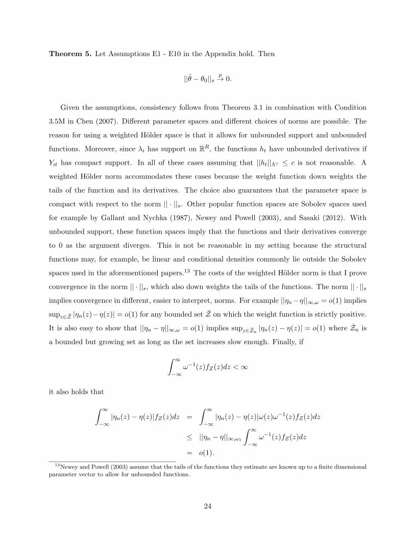
Theorem 5. Let Assumptions E1 - E10 in the Appendix hold. Then

||θ − θ0||sp→ 0.

Given the assumptions, consistency follows from Theorem 3.1 in combination with Condition

3.5M in Chen (2007). Different parameter spaces and different choices of norms are possible. The

reason for using a weighted Holder space is that it allows for unbounded support and unbounded

functions. Moreover, since λi has support on RR, the functions ht have unbounded derivatives if

Yit has compact support. In all of these cases assuming that ||ht||Λγ ≤ c is not reasonable. A

weighted Holder norm accommodates these cases because the weight function down weights the

tails of the function and its derivatives. The choice also guarantees that the parameter space is

compact with respect to the norm || · ||s. Other popular function spaces are Sobolev spaces used

for example by Gallant and Nychka (1987), Newey and Powell (2003), and Sasaki (2012). With

unbounded support, these function spaces imply that the functions and their derivatives converge

to 0 as the argument diverges. This is not be reasonable in my setting because the structural

functions may, for example, be linear and conditional densities commonly lie outside the Sobolev

spaces used in the aforementioned papers.13 The costs of the weighted Holder norm is that I prove

convergence in the norm || · ||s, which also down weights the tails of the functions. The norm || · ||s

implies convergence in different, easier to interpret, norms. For example ||ηn−η||∞,ω = o(1) implies

supz∈Z |ηn(z)−η(z)| = o(1) for any bounded set Z on which the weight function is strictly positive.

It is also easy to show that ||ηn − η||∞,ω = o(1) implies supz∈Zn |ηn(z) − η(z)| = o(1) where Zn is

a bounded but growing set as long as the set increases slow enough. Finally, if

∫ ∞−∞

ω−1(z)fZ(z)dz <∞

it also holds that

∫ ∞−∞|ηn(z)− η(z)|fZ(z)dz =

∫ ∞−∞|ηn(z)− η(z)|ω(z)ω−1(z)fZ(z)dz

≤ ||ηn − η||∞,ω1

∫ ∞−∞

ω−1(z)fZ(z)dz

= o(1).

13Newey and Powell (2003) assume that the tails of the functions they estimate are known up to a finite dimensionalparameter vector to allow for unbounded functions.

24

5.1.2 Semi-parametric estimator

Many different semiparametric approaches are possible in this setting. In this section, I describe

the approach I use in the application in Section 7. Detailed assumptions are listed in the appendix.

Here, I focus on the main assumptions, alternative implementations, and the main idea of the proof.

First I reduce the dimensionality of the optimization problem by assuming a location and scale

model for the conditional distribution of λi. In particular, I assume that

Fλi|Xi(λ;xi) = Fλ(Σ−1(xi, β1) (λ− µ(xi, β2)))

for a positive definite matrix Σ(xi, β1) ∈ RR×R and a vector µ(xi, β2) ∈ RR. The matrix Σ(xi, β1)

and the vector µ(xi, β2) are assumed to be known up to finite dimensional parameter vectors β1

and β2. The distribution function Fλ is unknown and its derivative is denoted by fλ. Furthermore,

I assume that Uit is independent of Xi and that the distribution of Uit is unknown. An alternative

to this assumption is to model the dependence between Uit and Xi to allow for heteroskedasticity.

Hence, both the distribution of λi | Xi and the distribution of Ui | Xi are semiparametric. An

alternative to a scale and location model is to assume that the support of Xi can be partitioned

into G groups and that fλi|Xi is the same for all Xi in group g. This approach is used by Weidner

(2011) in a panel data model where T →∞.

The structural functions can be parametric, semiparametric, or nonparametric depending on

the application. If the functions are parametric, I assume that ht(Yit, Xit) = h(Yit, Xit;β3t) where

h is known up to the finite dimensional parameter β3t, and h(Yit, Xit;β3t) is strictly increasing in

the first argument. One possibility is to set h(Yit, Xit;β3t) = h(Yit, β3t1)−X ′itβ3t2 where h(Yit, β3t1)

is a monotone transformation such as the Box-Cox transformation. It is also possible to specify

the function semiparametrically or nonparametrically, which leads to similar asymptotic properties

of the finite dimensional parameters of the model. For instance, in the previous example one

could assume that the transformation function is unknown, but strictly increasing and satisfies the

smoothness restrictions above.

Define β ≡ (β1, β2, β31, . . . , β3T , F )′ and assume that B is a compact subset of Rdβ . Also let

α ≡ (f1, . . . , fT , fλ) and θ ≡ (α, β). Denote the true parameter value by θ0 ≡ (α0, β0). The density

functions are assumed to satisfy similar smoothness assumptions as in the previous section.

In addition to the various finite dimensional parameters, only T one-dimensional densities as

well as one R-dimensional density function have to be estimated. Just as in the previous section,

25

these densities are estimated using the method of sieves. The norm is similar to the one used in

the previous section. The norm for the finite dimensional parameters is the standard Euclidean

norm. Therefore, the estimator θ = (α, β), which is the maximizer of the log-likelihood function, is

computationally almost identical to the one described in the previous section. The main difference

is that there are less sieve terms and more finite dimensional parameters to maximize over.

The appendix provides assumptions which ensure that the finite dimensional parameter vector

is estimated at a√n rate, and is asymptotically normally distributed. The arguments and proofs

are very similar to the ones in Ai and Chen (2003) and Carroll, Chen, and Hu (2010) among

others. The idea of the proof is to first introduce a weaker norm, namely the Fisher norm. Then,

I show that θ can be estimated at a rate faster than n−1/4 under this norm. Using this fast rate of

convergence in the weak norm and consistency in the strong norm, it can be shown that β converges

to β0 at a rate of n−1/2 and is asymptotically normal. In order to achieve this rate, the length of

the sieve has to be chosen in such a way that it balances the bias and the variance. Formally, I

obtain the following theorem.

Theorem 6. Assume that Assumptions E5 and E11 - E21 hold. Then

√n(β − β0

)d→ N

(0, (V ∗)−1

)where V ∗ is defined in equation (13) in the appendix.

Ackerberg, Chen, and Hahn (2012) provide a consistent estimator of the covariance matrix (V ∗)−1,

which is easy to implement.

5.1.3 Parametric estimator

Finally, given the results in the previous section, it is straightforward to estimate the model com-

pletely parametrically. The only additional assumption needed is that the densities fUit and fλi

are known up to a finite dimensional parameter vector. For example, one could assume that λi and

Ui are normally distributed, where the mean and the covariance of λi is a parametric function of

Xi and the variance of Uit is an unknown constant. This parameterization, which I also use in the

application, satisfies all identification assumptions. Various other parameterizations are of course

also possible. Consistency and asymptotic normality of the fully parametric maximum likelihood

estimator follows from standard arguments, such as those in Newey and McFadden (1986).

26

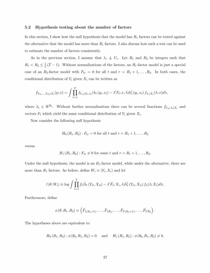
5.2 Hypothesis testing about the number of factors

In this section, I show how the null hypothesis that the model has R1 factors can be tested against

the alternative that the model has more than R1 factors. I also discuss how such a test can be used

to estimate the number of factors consistently.

As in the previous section, I assume that λi ⊥⊥ Ui. Let R1 and R2 be integers such that

R1 < R2 ≤ 12 (T − 1). Without normalizations of the factors, an R1-factor model is just a special

case of an R2-factor model with Ftr = 0 for all t and r = R1 + 1, . . . , R2. In both cases, the

conditional distribution of Yi given Xi can be written as

fYi1,...,YiT |Xi(y;x) =

∫ T∏t=1

fUit|Xi,λi(ht (yt, xt)− λ′Ft;x, λ)h′t (yt, xt) fλi|Xi(λ;x)dλ,

where λi ∈ RR2 . Without further normalizations there can be several functions fUit,λi|Xi and

vectors Ft which yield the same conditional distribution of Yi given Xi.

Now consider the following null hypothesis

H0 (R1, R2) : Ftr = 0 for all t and r = R1 + 1, . . . , R2

versus

H1 (R1, R2) : Ftr 6= 0 for some t and r = R1 + 1, . . . , R2.

Under the null hypothesis, the model is an R1-factor model, while under the alternative, there are

more than R1 factors. As before, define Wi ≡ (Yi, Xi) and let

l (θ,Wi) ≡ log

∫ T∏t=1

ft(ht (Yit, Xit)− λ′Ft;Xi, λ)h′t (Yit, Xit) fλ(λ;Xi)dλ.

Furthermore, define

φ (θ,R1, R2) ≡(F1(R1+1), . . . , F1R2 , . . . , FT (R1+1), . . . , FTR2

).

The hypotheses above are equivalent to

H0 (R1, R2) : φ (θ0, R1, R2) = 0 and H1 (R1, R2) : φ (θ0, R1, R2) 6= 0.

27

H0 (R1, R2) can be tested using a test statistic based on a scaled sample analog of

2

(supθ∈Θ

E[l (θ,Wi)]− supθ∈Θ:φ(θ,R1,R2)=0

E[l (θ,Wi)]

).

The intuition is that, under the null hypothesis, the difference above is equal to 0. Under the

alternative, the difference is strictly positive because the maximum of the unconstrained problem

is attained outside of the set where φ (θ,R1, R2) = 0. Furthermore, although not all features of the

model are point identified, the value of the likelihood at θ0 is identified. Define

LR (R1, R2) = 2

(supθ∈Θn

n∑i=1

l (θ,Wi)− supθ∈Θn:φ(θ,R1,R2)=0

n∑i=1

l (θ,Wi)

).

Chen, Tamer, and Torgovitsky (2011) show that, under the null hypothesis, LR (R1, R2) converges

in distribution to a supremum of a tight centered Gaussian process. They also prove that the

quantiles of the asymptotic distribution can be approximated consistently using a weighted boot-

strap. In a finite dimensional setup a similar result has been obtained by Lui and Shao (2003).

Let cα (R1, R2) denote the 1 − α quantile of the weighted bootstrap distribution. The test rejects

the null hypothesis if and only if LR (R1, R2) > cα (R1, R2). The following theorem is now a direct

consequence of the results in Chen, Tamer, and Torgovitsky (2011).

Theorem 7. Assume that Assumptions S2 - S8 and Assumptions 1 - 4 in Chen, Tamer, and

Torgovitsky (2011) hold. Also assume that λi ⊥⊥ Ui and that T ≥ 2R+ 1. Then:

(i) Under the null hypothesis LR (R1, R2) converges in distribution to a supremum of a tight

centered Gaussian process.

(ii) The likelihood ratio test has asymptotic size α:

P (LR (R1, R2) > cα (R1, R2) | H0 (R1, R2))→ α as n→∞.

(iii) The likelihood ratio test is consistent against any fixed alternative:

P (LR (R1, R2) > cα (R1, R2) | H1 (R1, R2))→ 1 as n→∞.

Remark 3. The Assumptions in Chen, Tamer, and Torgovitsky (2011) are directly applicable to the

28

setting in this paper but introducing them in detail would require a lot of notation and is therefore

omitted. Similarly, a more precise description of the asymptotic distribution is omitted.

Next, I assume that the true number of factors is at most R∗ where R∗ ≤ 12 (T − 1) is known.14

Let cn (R1, R∗) be a sequence of constants such that

cn (R1, R∗)

n→ 0 and

cn (R1, R∗)

log(log(n))→∞.

It now follows from the fact that LR (R1, R∗) converges to a supremum of a tight Gaussian process

under the null hypothesis and Theorem 1.3 in Dudley and Philipp (1983), which is a law of iterated

logarithm for empirical processes, that

P (LR (R1, R∗) > cn (R1, R

∗) | H0 (R1, R∗))→ 0 and

P (LR (R1, R∗) > cn (R1, R

∗) | H1 (R1, R∗))→ 1.

Let LR (R∗, R∗) = 0 and cn (R∗, R∗) > 0. Then the estimated number of factors is

R = min {R1 ∈ {0, . . . , R∗} : LR (R1, R∗) < cn (R1, R

∗)} .

The following theorem is a direct consequence of the previous derivation.

Theorem 8. Assume that Assumptions S2 - S8 and Assumptions 1 - 4 in Chen, Tamer, and

Torgovitsky (2011) hold. Also assume that λi ⊥⊥ Ui and that R ≤ R∗ ≤ 12 (T − 1). For any

R1 = 0, . . . , R∗ − 1 let cn (R1, R∗) be a sequence of constants that satisfies

cn (R1, R∗)

n→ 0 and

cn (R1, R∗)

log(log(n))→∞.

Let LR (R∗, R∗) = 0 and cn (R∗, R∗) > 0. Then P (R = R)→ 1.

Remark 4. In practice, the sequence cn (R∗, R∗) needs to be chosen. This is a very important issue

because for any given sample, the estimated number of factors directly follows from this sequence.

Selecting cn (R∗, R∗) with desirable finite sample properties, similar to the ones proposed by Bai

and Ng (2002) in linear factor models, is left for future research. In applications with small T , R∗

might be quite small. For instance, in the application in this paper, since T = 6 the upper bound

14A similar assumption is made in linear factor models; see for example Bai and Ng (2002).

29

for R∗ is 2. Hence, one might only be interested in testing whether R = 1 versus the alternative

that R = 2. In these cases, a test based on Theorem 7 might be more appealing than estimating

the number of factors consistently.

6 Monte Carlo simulation

In this section, I investigate the finite sample properties of the parametric and the semiparametric

estimator. I consider two setups with different shapes of the structural functions. In the first setup,

I am concerned with the finite sample properties of the finite dimensional parameters for various

distributions of Uit and different sample sizes. In the second setup, I replicate the distribution of

the data used in the next section and investigate finite sample properties of marginal effects.

6.1 Setup 1

I simulate the data from the model

(9)Y αit − 1

α= γ +X ′itβ + λ′iFt + Uit,

where Xit ∈ R4, λi ∈ R2, and T = 6. I assume that Xit1, Xit2 ∼ U [0, 1] and Xit3, Xit4 ∼ TN (0, 1),

where TN(0, 1) denotes the standard normal distribution truncated at −1 and 1. Furthermore,

λi ∼ N (µ(Xi, θ),Σ) with

Σ =

0.5 0.25

0.25 0.5

, µ(Xi, θ) =

Xi·1θ1 + Xi·3θ3

Xi·2θ2 + Xi·4θ4

, and Xi·k =1

T

T∑t=1

Xitk.

The interpretation is that both skills depend linearly on two of the covariates. I vary the distribution

of Uit, which is either (i) Normal, (ii) Gamma with scale parameter 1 and shape parameter 5, (iii)

Student’s t with 5 degrees of freedom, or (iv) Logistic. Each distribution is standardized such that

the median equals 0 and the standard deviation is 0.5. I assume that Ui ⊥⊥ (Xi, λi). These four

error distributions cover many interesting cases. The first and last are standard and commonly

used distributions while the Gamma distribution is asymmetric and the Student’s t distribution

does not have exponentially decreasing tails. I assume that

β =(

0.5 0.8 −0.5 0.2)′, θ =

(0.5 −0.3 0.3 0.4

)′, and

30

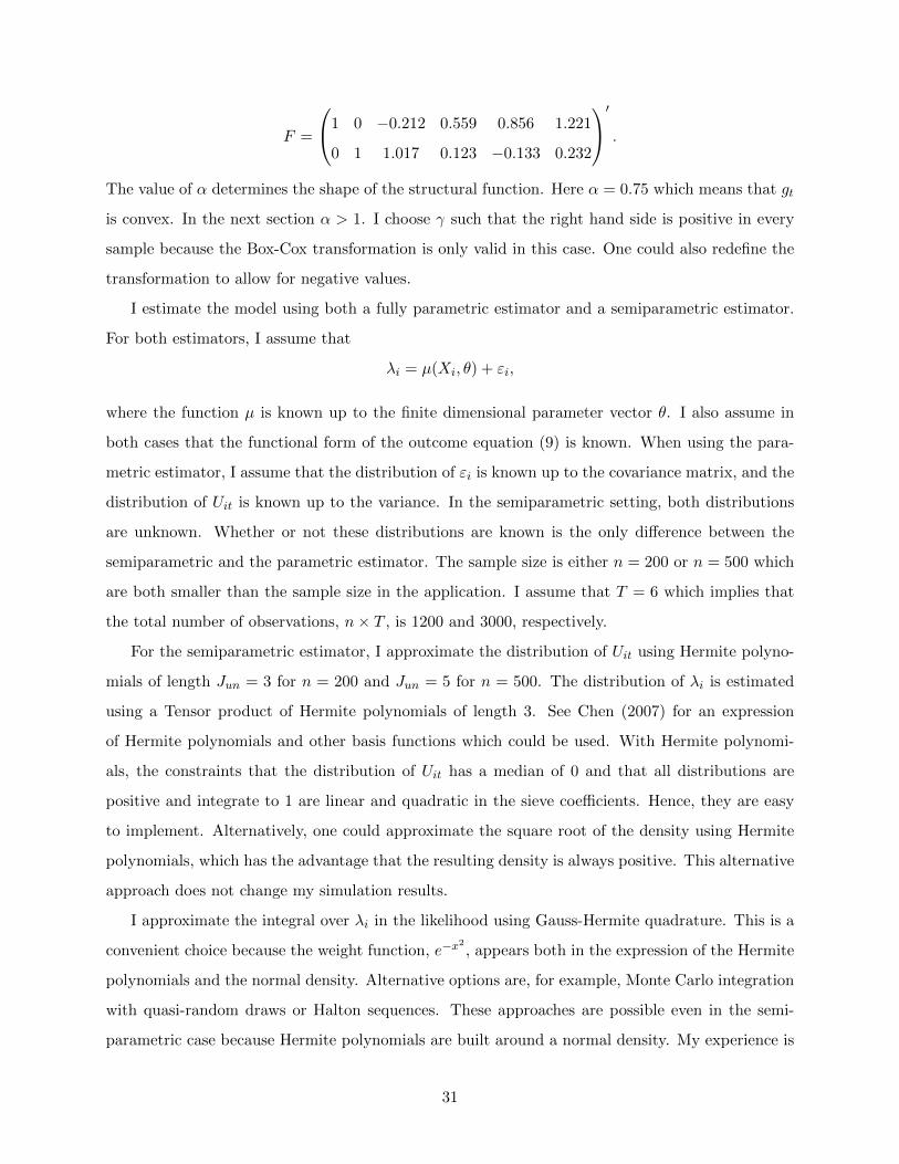
F =

1 0 −0.212 0.559 0.856 1.221

0 1 1.017 0.123 −0.133 0.232

′ .The value of α determines the shape of the structural function. Here α = 0.75 which means that gt

is convex. In the next section α > 1. I choose γ such that the right hand side is positive in every

sample because the Box-Cox transformation is only valid in this case. One could also redefine the

transformation to allow for negative values.

I estimate the model using both a fully parametric estimator and a semiparametric estimator.

For both estimators, I assume that

λi = µ(Xi, θ) + εi,

where the function µ is known up to the finite dimensional parameter vector θ. I also assume in

both cases that the functional form of the outcome equation (9) is known. When using the para-

metric estimator, I assume that the distribution of εi is known up to the covariance matrix, and the

distribution of Uit is known up to the variance. In the semiparametric setting, both distributions

are unknown. Whether or not these distributions are known is the only difference between the

semiparametric and the parametric estimator. The sample size is either n = 200 or n = 500 which

are both smaller than the sample size in the application. I assume that T = 6 which implies that

the total number of observations, n× T , is 1200 and 3000, respectively.

For the semiparametric estimator, I approximate the distribution of Uit using Hermite polyno-

mials of length Jun = 3 for n = 200 and Jun = 5 for n = 500. The distribution of λi is estimated

using a Tensor product of Hermite polynomials of length 3. See Chen (2007) for an expression

of Hermite polynomials and other basis functions which could be used. With Hermite polynomi-

als, the constraints that the distribution of Uit has a median of 0 and that all distributions are

positive and integrate to 1 are linear and quadratic in the sieve coefficients. Hence, they are easy

to implement. Alternatively, one could approximate the square root of the density using Hermite

polynomials, which has the advantage that the resulting density is always positive. This alternative

approach does not change my simulation results.

I approximate the integral over λi in the likelihood using Gauss-Hermite quadrature. This is a

convenient choice because the weight function, e−x2, appears both in the expression of the Hermite

polynomials and the normal density. Alternative options are, for example, Monte Carlo integration

with quasi-random draws or Halton sequences. These approaches are possible even in the semi-

parametric case because Hermite polynomials are built around a normal density. My experience is

31

that Gauss-Hermite quadrature leads to slightly better finite sample properties.

Table 1 provides finite sample properties for estimates of α, β1, and θ1. Different values of α

yield very similar results and are therefore not reported. The parameters α, β1, and θ1 cover dif-

ferent aspects of the model. The parameter α measures the nonlinearity of the structural function,

β1 is one of the coefficients of the regressor, and θ1 is a parameter of the distribution of λi | Xi.

The results for the other parameters are very similar. I focus on the mean and the root mean

square error (RMSE) of the estimated parameters. All results are based on 1000 Monte Carlo

iterations. The fully parametric model has very good finite sample properties. For all values of α

and all distributions of Uit, both the bias and the RMSE are small and the RMSE decreases with

the sample size. According to the asymptotic approximation, the RMSE with n = 200 should be√5/2 ≈ 1.58 times larger than the RMSE with n = 500, which is roughly true in the parametric

case. In the semiparametric case, this is only approximately the case if Uit is either logistically or

normally distributed. Clearly, the fully parametric estimator has better finite sample properties

compared to the semiparametric estimator. However, the semiparametric estimator performs quite

well for all distributions even in relatively small samples. The semiparametric estimator achieves

its best results for the normal distribution. This is not surprising since the Hermite polynomials

are built around a normal density. The estimator performs well even in the case of an asymmetric

error distribution if the size of the sieve is long enough as in the case of the Gamma distribution.

With n = 200 and Jun = 3, the estimates are substantially biased. This bias mostly disappears

with n = 500 and Jun = 5. The Student-t and logistic distribution have fatter tails, which results

in more variation of the estimates relative to the normal distribution.

6.2 Setup 2

The second setup mimics the data and the model used in the application. Now

Y αit − 1

α= γ +Xitβt + Zitδt + λ′iFt + Uit,

where Xit, Zit ∈ R, λi ∈ R2, and T = 6. Moreover, Xit = Xi1 for all t = 1, 2, 3 and Xit = Xi4 for all

t = 4, 5, 6. The same holds for Zit. I assume that Xit and Zit have truncated normal distributions.

The means, the covariance matrix, and the cutoffs are chosen such that the distributions closely

mimic the empirical distributions of the teaching practice measures in the application.15 The

15The regressors Xit and Zit correspond to the traditional and modern teaching practice measure, respectively.In the application t = 1, 2, 3 belongs to mathematics and t = 4, 5, 6 belongs to science test scores. Nonparametric

32

Table 1: Mean and root-MSE for α, β1, and θ1

α = 0.75 β1 = 0.5 θ1 = 0.5

Mean RMSE Mean RMSE Mean RMSE

Uit ∼ Normal - SPMLE

n = 200 0.748 0.049 0.505 0.098 0.497 0.253

n = 500 0.750 0.040 0.505 0.075 0.515 0.160

Uit ∼ Normal - MLE

n = 200 0.746 0.046 0.500 0.094 0.487 0.238

n = 500 0.748 0.033 0.501 0.066 0.503 0.148

Uit ∼ Gamma - SPMLE

n = 200 0.583 0.173 0.306 0.202 0.320 0.232

n = 500 0.694 0.066 0.426 0.091 0.427 0.146

Uit ∼ Gamma - MLE

n = 200 0.742 0.046 0.493 0.085 0.515 0.230

n = 500 0.745 0.032 0.494 0.057 0.491 0.142

Uit ∼ Student’s t - MMLE

n = 200 0.784 0.109 0.598 0.330 0.612 0.502

n = 500 0.776 0.089 0.576 0.251 0.589 0.296

Uit ∼ Student’s t - MLE

n = 200 0.741 0.062 0.498 0.114 0.499 0.254

n = 500 0.745 0.048 0.499 0.091 0.505 0.162

Uit ∼ Logistic - SMLE

n = 200 0.784 0.060 0.531 0.121 0.559 0.283

n = 500 0.752 0.044 0.507 0.082 0.510 0.163

Uit ∼ Logistic - MLE

n = 200 0.741 0.053 0.504 0.104 0.523 0.248

n = 500 0.748 0.036 0.499 0.069 0.497 0.153

The number of Monte Carlo simulations is 1000. The true value of α, β1, and θ1 are 0.75, 0.5,

and 0.5 respectively. The distribution of Uit is approximated using Hermite polynomials of

length Jun = 3 for n = 200 and Jun = 5 for n = 500. The distribution of λi is approximated

using a tensor product of Hermite polynomials of length 3.

33

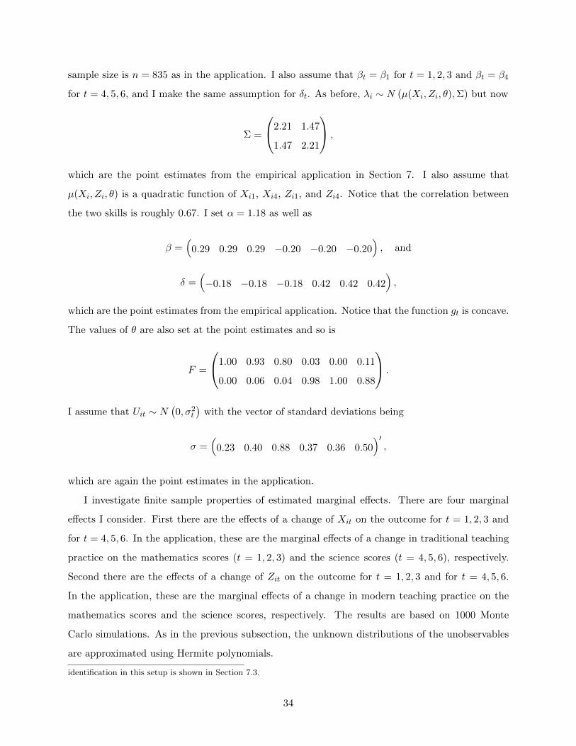
sample size is n = 835 as in the application. I also assume that βt = β1 for t = 1, 2, 3 and βt = β4

for t = 4, 5, 6, and I make the same assumption for δt. As before, λi ∼ N (µ(Xi, Zi, θ),Σ) but now

Σ =

2.21 1.47

1.47 2.21

,

which are the point estimates from the empirical application in Section 7. I also assume that

µ(Xi, Zi, θ) is a quadratic function of Xi1, Xi4, Zi1, and Zi4. Notice that the correlation between

the two skills is roughly 0.67. I set α = 1.18 as well as

β =(

0.29 0.29 0.29 −0.20 −0.20 −0.20), and

δ =(−0.18 −0.18 −0.18 0.42 0.42 0.42

),

which are the point estimates from the empirical application. Notice that the function gt is concave.

The values of θ are also set at the point estimates and so is

F =

1.00 0.93 0.80 0.03 0.00 0.11

0.00 0.06 0.04 0.98 1.00 0.88

.

I assume that Uit ∼ N(0, σ2

t

)with the vector of standard deviations being

σ =(

0.23 0.40 0.88 0.37 0.36 0.50)′,

which are again the point estimates in the application.

I investigate finite sample properties of estimated marginal effects. There are four marginal

effects I consider. First there are the effects of a change of Xit on the outcome for t = 1, 2, 3 and

for t = 4, 5, 6. In the application, these are the marginal effects of a change in traditional teaching

practice on the mathematics scores (t = 1, 2, 3) and the science scores (t = 4, 5, 6), respectively.

Second there are the effects of a change of Zit on the outcome for t = 1, 2, 3 and for t = 4, 5, 6.

In the application, these are the marginal effects of a change in modern teaching practice on the

mathematics scores and the science scores, respectively. The results are based on 1000 Monte

Carlo simulations. As in the previous subsection, the unknown distributions of the unobservables

are approximated using Hermite polynomials.

identification in this setup is shown in Section 7.3.

34

Table 2 shows the means of the estimated marginal effects for different estimation methods.

All marginal effects are evaluated at the median values of Xit, Zit, and of the unobservables. The

first line contains the true marginal effects, which are very close the estimated marginal effects in

the application. The second line shows the marginal effects when a standard linear fixed effects

model is used for estimation. For t = 1, 2, 3, the estimated marginal effects have the right signs but

the estimates are considerably biased downwards in absolute value. For t = 4, 5, 6, the estimates

are far from the true values. It appears as if Xit has a positive effect on the outcome, although

the true effect is negative. Both the parametric model and the semiparametric two factor model

yield estimated marginal effects that are close to the true values, with the parametric estimator

performing better on average.

Table 2: Mean of estimated marginal effects

t = 1, 2, 3 t = 4, 5, 6

Xit Zit Xit Zit

True marginal effect 0.186 -0.112 -0.132 0.269

Linear fixed effects 0.074 -0.009 0.044 0.020

Parametric - two factor 0.181 -0.108 -0.134 0.270

Semiparametric - two factors 0.172 -0.099 -0.113 0.235

Table 3 displays the root means square error (RMSE) of the estimates. The estimates from the

linear model have a large RMSE compared to the two factor models. The difference is especially

large for t = 4, 5, 6. The parametric and the semiparametric two factor models yield very similar

results.

Table 3: RMSE of estimated marginal effects

t = 1, 2, 3 t = 4, 5, 6

Xit Zit Xit Zit

Linear fixed effects 0.116 0.107 0.178 0.250

Parametric - two factor 0.062 0.066 0.068 0.090

Semiparametric - two factors 0.063 0.063 0.069 0.091

35

7 Application

In this section I use the static factor model to investigate the relationship between teaching practice

and student achievement. I use test scores of students from the Trends in International Mathematics

and Science Study (TIMSS) as outcome variables. This study is linked to a student questionnaire,

which allows me to calculate a measure of modern teaching practice and a measure of traditional

teaching practice for each class a student attends. Modern teaching practice is associated with

group work and reasoning, while traditional teaching practice is based on lectures and memorizing.

The two measures are defined below. A standard linear fixed effects model controls for a scalar

unobserved ability term, which has the same effect on all outcomes. This assumption means, loosely

speaking, that if two students, A and B, have the same observed characteristics and student A is

better in subject 1, then student A must also be better in subject 2. Furthermore, the impact of the

teaching practice on student achievement is, by assumption, the same for all levels of unobserved

ability. These assumptions can be relaxed by using the factor model described in this paper.

Linear fixed effects models are often used in similar settings to control for unobserved ability.

Bietenbeck (2011) and Lavy (2011) study the relationship between teaching practice and student

achievement. Dee (2007) analyzes whether the teacher’s gender has an influence of student achieve-

ment. Clotfelter, Ladd, and Vigdor (2010) investigate the relationship between teacher credentials

and student achievement. In all these papers, the T dimension in the panel are different subjects.

Aucejo (2011) studies teacher effectiveness and allows for student-teacher interactions with a scalar

student fixed effect. Although a nonlinear factor model, which controls for multiple abilities, seems

attractive in these settings, it should be noted that such a model is only applicable if T ≥ 5.

In this application, I make use the definitions of traditional and modern teaching practice by

Bietenbeck (2011). The main difference in my paper is the model used to estimate the parameters

of interest. Moreover, I use different test scores as outcome variables and the sample differs slightly

as explained below.

7.1 Data

TIMSS is an international assessment of mathematics and science knowledge of fourth and eighth-

grade students. It is carried out every four years. I make use of the 2007 sample of eighth-grade

students in the United States. This sample consists of 7377 students in 235 schools. Each student

attends a mathematics and an integrated science class with different teachers in each of the two

36

classes for almost all students. I exclude students which cannot be linked to their teachers, students

in classes with less than three students, as well as observations with missing values in the teaching

practice variables or control variables (defined below). This reduction leaves 4642 students in 182

schools. This is the estimation sample of Bietenbeck (2011), who provides more details on the data.

I further restrict myself to white, American born students between the age of 13.5 and 15.5 with

English as their first language. I also restrict the sample to schools with an enrollment between 100

and 600 students, where parents’ involvement is not reported to be very low, and where less than

75% of the students receive free lunch. The resulting sample consists of 835 male and 935 female

students in 99 schools with 144 mathematics and 161 science teachers.16

In addition to the overall test score for mathematics and science, the TIMSS contains test

scores for different cognitive domains of the tests which are mathematics knowing, applying and

reasoning, as well as science knowing, applying and reasoning. I use these six test scores as the

dependent variables Yit, where i denotes a student and t denotes a test. Hence, T = 6 which allows

me to estimate a factor model with two factors. The main regressors are the measures of teaching

practice. To construct these, I use the student questionnaire where students are asked questions

about how often they do certain activities in class. The answers are on a four point scale with 1

corresponding to never, 2 to some lessons, 3 to about half of the lessons, and 4 to every or almost

every lesson. The exact questions about class activities, which are used to construct the measures,

are listed in Table 6. These particular questions are used because they can be unambiguously

matched to recommendations on teaching practices in Zemelman, Daniels, and Hyde (2005). These

recommendations are based on a survey of the standards movement in teaching practices literature

and categorize teaching methods as either to be increased or to be decreased. In Table 6, questions

belonging to traditional teaching are the ones labeled to be decreased in Zemelman et al. (2005),

while questions belonging to modern teaching are labeled to be increased.17 For each student and

each class I compute the mean response of the answers in the modern and traditional category. I

then calculate class means of these averages, excluding the student’s own response. These class

means are the measures of traditional and modern teaching practice faced by student i in the

mathematics and science class.18 These measures therefore range from 1 to 4. In addition to

these teaching measures, I control for class size, hours spent in class, teacher experience, whether

a teacher is certified in the field, and the gender of the teacher.

16All results are very similar in different samples, such as the sample without conditioning on the school variables.17See Bietenbeck (2011) for more details on the teaching practice measures and background literature.18The results are very similar when I include the student’s own response when constructing the teaching measures.

37

7.2 Model and implementation

The results reported in this paper are based on the outcome equation

Y αit − 1

α= γ +Xmod

it βmodt +Xtradit βtradt + Z ′itγt + λ′iFt + Uit,(10)

where t = 1, 2, 3 corresponds to the mathematics scores (knowing, applying, reasoning) and t =

4, 5, 6 to the science scores (knowing, applying, reasoning). The scalars Xmodit and Xtrad

it are the

modern and traditional teaching practice measures of the classes which student i attends. I assume

that

βtrad1 = βtrad2 = βtrad3 and βtrad4 = βtrad5 = βtrad6 .

I make an analogous assumption for βmodt . Hence, I allow traditional and modern teaching practice

to have a different impact on mathematics and science subjects, but the same impact across cogni-

tive domains. The vector Zit includes class size, hours spent in class, teacher experience, whether

a teacher is certified in the field, and the gender of the teacher. I assume that

λi = µ(Xi, θ) + εi,

where εi ⊥⊥ Xi and µ is a quadratic function of Xmodi and Xtrad

i but does not include interactions of

these regressors.19 I also assume that Ui ⊥⊥ (λi, Xi). I implemented various specifications, none of

which change the main conclusions. These different specifications include adding nonlinear terms

of Xi and Zi to the right hand side of equation (10), assuming that the covariance matrix of εi is

a parametric function of Xi, allowing λi to depend on Zi, and allowing β to differ across all t.

In the most general model I estimate, the distributions of Uit and εi are unspecified and esti-

mated with Hermite polynomials of order 5 and a tensor product of Hermite polynomials of order

3, respectively. Changing the order does not affect the results much. I also estimate different

parametric models assuming that εi and Uit are normally distributed with an unknown covariance

matrix and an unknown variance, respectively. In particular, I estimate a parametric two factor

model, as well as a parametric one factor model and a parametric one factor model with Ft = 1. In

all of these models, I use the functional form assumptions above. The estimates are compared to the

ones obtained from a linear fixed effects model. All integrals are approximated using Gauss-Hermite

quadrature.

19With this assumption, λi become correlated random effects instead of fixed effects.

38

7.3 Nonparametric identification

Although a semiparametric model is used in this application, the structural functions are nonpara-

metrically identified, under the assumptions of Theorem 1. Nonparametric identification might not

be immediately obvious from Theorem 1 because Zit = Zi1 for t = 1, 2, 3 and Zit = Zi4 for t = 4, 5, 6.

The same is true for Xmodit and Xtrad

it . To simplify the notation, define Xit ≡(Xmodit , Xtrad

it , Zit).

First let Xi5 = Xi6 = x6 as in Theorem 1. Hence also Xi4 = x6. If fXi1,Xi6 (x1, x6) > 0 for all

x1 ∈ X1, it follows immediately from Theorem 1 that ht is identified for all xt ∈ Xt and t = 1, 2, 3.

Now assume that for some x1 it holds that fXi1,Xi6 (x1, x6) > 0 for all x6 ∈ X6. Then, just as in

the discussion after Theorem 1, we can switch roles of t = 1, 2, 3 and t = 4, 5, 6 and identify ht for

all xt ∈ Xt and t = 4, 5, 6.

To achieve these identification results, it is not necessary that fXi1,Xi6 (x1, x6) > 0 for all

x1 ∈ X1. For example, assume that all components of Xit are continuously distributed. Further-

more, assume that for all x and some δ > 0 it holds that fXi1,Xi6 (x1, x) > 0 and fXi1,Xi6 (x, x6) > 0

for all x1, x6 ∈ [x− δ, x+ δ]. This assumption is reasonable in this application. It says that if the

traditional teaching measure in the mathematics class has the value x, then all values in the interval

[x− δ, x+ δ] are possible values for the traditional teaching measure in the science class. A similar

statement has to be true for the modern teaching measure. With these assumptions, Theorem 1

yields identification of ht for all xt ∈ [x− δ, x+ δ] and t = 1, 2, 3. Switching roles of t = 1, 2, 3 and

t = 4, 5, 6 shows identification of ht for all xt ∈ [x−2δ, x+2δ] and t = 4, 5, 6. Switching roles again,

it then follows that ht is identified for all xt ∈ [x− 3δ, x+ 3δ] and t = 1, 2, 3. Since this process can

be iterated, the functions ht are identified for all t and for all xt ∈ Xt.

Next to identifying the structural functions, the distribution of λi | Xi is identified using similar

arguments. However, note that this conditional distribution is not identified for all x ∈ X1×· · ·×X6.

The reason is that Xi1 = Xi2 = Xi3 and Xi4 = Xi5 = Xi6 for all i and thus, the distribution of

λi | Xi is only identified for values of Xi for which these equalities hold.

7.4 Results

Table 4 contains the estimation results for the sample of 835 boys.20 The table shows marginal

effects of an increase in teaching practice evaluated at the median levels of the regressors and the

20Since each student only answers a random sample of test questions, the TIMSS data set contains five imputedvalues. I use the first imputed value, but the results based on the other ones are similar. The standard errors do notaccount for imputation of missing values. Furthermore, all issues caused by the fact that the teaching measures aregenerated regressors are ignored.

39

unobservables. In a linear model, these marginal effects are equal to the four coefficients βmodt

and βtradt with t = 1 and t = 4. First consider the results of the linear fixed effects model in the

first row. Using this model, I find a positive relationship between traditional teaching practice

and student achievement in both subjects. The relationship between modern teaching practice and

science scores is also positive but insignificant. These results are in line with findings in Bietenbeck

(2011) and Lavy (2011). Bietenbeck (2011) mainly finds a positive relationship between traditional

teaching practice and student achievement while Lavy (2011) finds evidence of positive effects of

both modern and traditional elements. I standardized Yit and the teaching practice measures

to have a standard deviation of 1. Hence, the economic interpretation is that a one standard

deviation increase of tradition practice is associated with a 0.085 standard deviation increase in the

mathematics test score.

Table 4: Marginal effects teaching practice for boys

Math scores Science scores

Traditional Modern Traditional Modern

Linear fixed effects 0.085*** -0.002 0.040* 0.027

Parametric - one factor - Ft = 1 0.087*** -0.005 0.045*** 0.027**

Parametric - one factor 0.126*** -0.032* 0.093*** -0.015

Parametric - two factors 0.188*** -0.114** -0.134** 0.265***

Semiparametric - two factors 0.165*** -0.137** -0.145** 0.236***

The symbols *, **, and *** denote significance at 10%, 5%, and 1% level respectively.

The next line shows marginal effects for a parametric one factor model with Ft = 1. The

marginal effects, evaluated at median values, are very similar to the linear model. This is expected

since the models are very similar. Notice that in the linear model, the relation between λi and Xi

is not modeled. Hence, a large difference in these marginal effects could be due to misspecification

of this relationship while the similarity suggests that the relationship is well specified. Allowing Ft

to vary produces different marginal effects as shown in the third line. The results still suggest that

traditional teaching practices are associated with better test scores in both subjects.

A parametric two factor model yields very different results. I still find a positive relationship

between traditional teaching practice and mathematics scores, but a positive relationship between

modern teaching practice and science scores. The two other marginal effects are significantly

40

negative. Finally, the semiparametric model yields similar results as the parametric two factor

model. Results for the sample of 935 girls are given in Appendix E and are qualitatively similar.

The semiparametric model also provides an estimate of the distribution of λi. Figure 1 shows

level curves of this distribution at the median level of Xi. The correlation between the two skills

is around 60%. In the parametric model, the estimated correlation is around 67%. It is also

interesting to look at the estimated factors from the semiparametric model which are

F =

1.00 0.94 0.81 0.04 0.00 0.13

0.00 0.06 0.04 0.97 1.00 0.88

.

The rows correspond to the two different factors and columns to the different subject. The first

column belongs to mathematics knowing, and columns 2−6 to mathematics applying, mathematics

reasoning, science knowing, science applying and science reasoning, respectively. The mathematics

subjects have more weights on the first skill, while science subjects have more weight on the second

skill. Notice that two numbers are exactly 0 and two are exactly 1, which corresponds to a particular

normalization.

Figure 1: Level curves skill distribution

Using the results from Section 5.2, I can test the parametric one factor model against the

parametric two factor model, and the semiparametric one factor model against the semiparametric

41

two factor model. In both cases, the null hypothesis is a one factor model and the alternative is a

two factor model. Both null hypotheses are rejected at any significance level greater than 0.5%.

The conclusions one can draw from using a nonlinear model are illustrated in Table 5. This

table contains marginal effects, using the semiparametric two factor model, for different values of

the skill distribution. High skills means being two standard deviations above the median value

in both dimensions, and low skills means being two standard deviations below. The estimated

coefficient measuring nonlinearity, α, is equal to 1.221 with a standard error of 0.062. Hence, the

estimate is significantly different from 1. In the table it can be observed that the marginal effects

are larger in absolute value for students with lower abilities. This means that the teaching method

seems to have a larger influence on students with low ability. The difference in the marginal effects

between the high and the low skilled students is more than 20%.

Table 5: Marginal effects teaching practice for boys

Math scores Science scores

Traditional Modern Traditional Modern

Low skill 0.185 -0.154 -0.163 0.265

Median skill 0.165 -0.137 -0.145 0.236

High skill 0.154 -0.128 -0.135 0.220

These marginal effects are based on the semiparametric two factor

model. They are evaluated at the median of the observables.

8 Conclusion

In this paper, I consider identification and estimation of nonparametric panel data models with

multidimensional, unobserved individual effects. The models have two key distinguishing features.

First, the setup allows for the various unobserved individual effects to impact outcomes differently

in different time periods. Individual effects often represent unobserved ability, in which case the

model permits the returns to ability to change over time. Second, the models allows for heteroge-

neous marginal effects of the covariates on the outcome, which implies, for example, that returns

to education may depend on unobserved ability.

I present nonparametric point identification conditions for all parameters of the models. These

parameters include the structural functions as well as the number of factors, the factors themselves,

42

and the distributions of the unobservables, λi and Uit, conditional on the regressors. The identi-

fication results imply identification of average effects as well as marginal effects, which are often

the main objects of interest in applications. I consider different settings with both discrete and

continuous outcomes as well as a dynamic model with lagged dependent variables as regressors.

After providing sufficient conditions for identification, I present a nonparametric maximum likeli-

hood estimator which allows estimating the structural functions, the factors, and the conditional

distribution of (λi, Ui) consistently. The estimator requires estimating functions which might be

high dimensional in applications, such as the conditional density of λi. Therefore, in addition to

a fully nonparametric estimator, this paper provides a flexible semiparametric estimator. In this

setup, the dimensions of the conditional densities are reduced by modeling them as a location and

scale model. The structural functions can be nonparametric, semiparametric, or parametric. In the

latter two cases, many parameters of interest are finite dimensional. I show that these estimated

finite dimensional parameters are√n consistent and asymptotically normally distributed. An easy

to implement fully parametric estimator is also described. Finally, I discuss how the null hypothesis

that the model has R factors can be tested against the alternative that the model has more than

R factors, and how this result can be used to estimate the number of factors consistently. I show

in Monte Carlo experiments that the semiparametric estimator performs well in finite samples.

I use the semiparametric estimator to investigate the relationship between teaching practice

and student achievement. The outcome variables Yit are different mathematics and science test

scores for each student i. The main regressors are a measure of traditional teaching practice and

a measure of modern teaching practice for each class a student attends. These measures are con-

structed using students’ answers to questions about class activities. A linear fixed effects estimator

is commonly used in related applications. This model controls for a scalar unobserved ability term,

which has the same effect on all outcomes. Furthermore, the impact of the teaching practice on

student achievement is, by assumption, the same for all levels of unobserved ability. With this

model, I find a positive relationship between traditional teaching practice and test outcomes in

both mathematics and science. I then estimate a nonlinear two factor model and obtain substan-

tially different results. I still find a positive relationship between traditional teaching practice and

mathematics test scores, but a positive relationship between modern teaching practice and science

test scores. Furthermore, the structural functions are significantly nonlinear. In particular, the

magnitude of the relationship between teaching practice and test outcomes is higher for students

with low abilities than for students with high abilities.

43

Appendices

A Proofs and examples static continuous factor model

A.1 Proof of Lemma 1

First condition on Xi ∈ X and suppress Xi. Now notice that Zi1 and ZiK are independent

conditional on λi. Therefore

P (Zi1 < s1, ZiK < sK) = Eλi [P (Zi1 < s1 | λi)P (ZiK < sK | λi)]

=

∫P (Zi1 < s1 | λi = λ)P (ZiK < sK | λi = λ) fλi(λ)dλ.

Moreover,

fZi1,ZiK (s1, sK) =

∫fZi1|λi(s1;λ)fZiK |λi(sK ;λ)fλi(λ)dλ

It follows that for any bounded function m such that E[|m(Zi1)|] <∞∫fZi1,ZiK (s1, sK)m(s1)ds1 =

∫fZiK ,λi(sK , λ)

(∫fZi1|λi(s1;λ)m(s1)ds1

)dλ.

From Theorem 2.1 in Mattner (1993) and Theorem 2.1 in D’Haultfoeuille (2011) it now follows that

Zi1 is bounded complete for λi. Furthermore, Proposition 2.4 in D’Haultfoeuille (2011) implies that

λi is (bounded) complete for ZiK and that λi is (bounded) complete for Zi1. Hence, by the previous

equality, Zi1 is bounded complete for ZiK .

A.2 Proof of Theorem 1

First condition on Xi ∈ X such that Xit = xt for all t = R+2, . . . , 2R+1. To simplify the notation,

I suppress Xit in the function ht in the proof. Define

LR =

{m : RR → R :

∫RR|m(v)|dv <∞

}and

LRbnd =

{m ∈ LR : sup

v∈RR|m(v)| <∞

}.

Furthermore define

LR(Z1) ≡{m : RR → R :

∫RR|m(v)|fZi1(v)dv <∞

}LRbnd(Z1) ≡

{m ∈ LR(Z1) : sup

v∈RR|m(v)| <∞

}

44

as well as LR(ZK), LRbnd(ZK), LR(Λ), and LRbnd(Λ) analogously. Now let skR+1∈ R be a fixed

constant and define the operators

L1,kR+1,K : LRbnd(ZK)→ LRbnd(L1,kR+1,Km

)(s1, skR+1

) ≡∫fZi1,ZiK ,ZikR+1

(s1, sK , skR+1)m(sK)dsK

L1,K : LRbnd(ZK)→ LRbnd

(L1,Km) (s1) ≡∫fZi1,ZiK (s1, sK)m(sK)dsK

L1,λ : LRbnd → LRbnd

(L1,λm) (s1) ≡∫fZi1|λi(s1;λ)m(λ)dλ

Lλ,K : LRbnd(ZK)→ LRbnd

(Lλ,Km) (λ) ≡∫fZiK ,λi(sK , λ)m(sK)dsK

DkR+1,λ : LRbnd(Λ)→ LRbnd(Λ)(DkR+1,λm

)(skR+1

, λ) ≡ fZikR+1|λi(skR+1

;λ)m(λ).

The operator L1,kR+1,K should be seen as a mapping from LRbnd(ZK) to LRbnd for a fixed value skR+1.

Changing the value of skR+1gives a different mapping. With these definitions for any m ∈ LRbnd(ZK)

(L1,K,kR+1

m)

(s1, skR+1)

=

∫fZi1,ZiK ,ZikR+1

(s1, sK , skR+1)m(sK)dsK

=

∫ (∫fZi1|λi(s1;λ)fZiK |λi(sK ;λ)fZikR+1

|λi(skR+1;λ)fλ(λ)dλ

)m(sK)dsK

=

∫fZi1|λi(s1;λ)fZikR+1

|λi(skR+1;λ)

(∫fZiK ,λi(sK , λ)m(sK)dsK

)dλ

=

∫fZi1|λi(s1;λ)fZikR+1

|λi(skR+1;λ) (Lλ,Km) (λ)dλ

=

∫fZi1|λi(s1;λ)

(DkR+1,λLλ,Km

)(skR+1

, λ)dλ

=(L1,λDkR+1,λLλ,Km

)(s1, skR+1

).

Similarly,

(L1,Km) (s1) = (L1,λLλ,Km) (s1).

Since these equalities hold for all functions m ∈ LRbnd(ZK) it follows that

L1,kR+1,K = L1,λDkR+1,λLλ,K

45

and

L1,K = L1,λLλ,K .

By Assumption S8, L1,λ is invertible and the inverse can be applied from the left. Therefore

L−11,λL1,K = Lλ,K ,

which implies that

L1,kR+1,K = L1,λDkR+1,λL−11,λL1,K .

Lemma 1 of Hu and Schennach (2008) and Assumption S8 imply that L1,K has a right inverse

which is densely defined on LRbnd. Therefore,

L1,kR+1,KL−11,K = L1,λDkR+1,λL

−11,λ.

The operator on the left hand side depends on the population distribution of the observables

only. Hence, it can be considered known. Hu and Schennach (2008) deal with the same type of

operator equality in a measurement error setup. They show that the operator on the left hand

side is bounded and its domain can therefore be extended to LRbnd. They also show that the right

hand side is an eigenvalue-eigenfunction decomposition of the known operator L1,kR+1,KL−11,K . The

eigenfunctions are fZi1|λi(s1;λ) with corresponding eigenvalues fZikR+1|λi(skR+1

;λ). Each λ indexes

an eigenfunction and an eigenvalue. The eigenfunctions are functions of s1 and skR+1is a fixed

constant. Hu and Schennach (2008) show that this decomposition is unique up to three nonunique

features:

1. Scaling: Multiplying each eigenfunction by a constant yields a different eigenvalue-eigenfunction

decomposition belonging to the same operator L1,kR+1,KL−11,K .

2. Eigenvalue degeneracy: If two or more eigenfunctions share the same eigenvalue, any linear

combination of these eigenfunctions are also eigenfunctions. Then several different eigenvalue-

eigenfunction decompositions belong to the same operator L1,kR+1,KL−11,K .

3. Ordering: For λ that satisfies λ = B(λ) for any one to one transformation B : RR → RR

L1,λDkR+1,λL−11,λ = Lλ,1DkR+1,λ

L−1

λ,1.

These conditions are very similar to conditions for nonuniqueness of an eigendecomposition of a

square matrix. While for matrices the order of the columns of the matrix that contains the eigenvec-

tors is not fixed, with operators any one to one transformation of λ leads to an eigendecomposition.

I show next that, given the assumptions of the theorem, the scaling and the ordering are fixed

by assumption. Furthermore, all eigenvalues are unique. It then follows that there are unique

operators L1,λ and DkR+1,λ such that L1,kR+1,KL−11,K = L1,λDkR+1,λL

−11,λ.

46

In now verify that these three nonunique features cannot occur in my model. First, the scaling

is unambiguous because all eigenfunctions have to integrate to one. Second, I show that eigenvalue

degeneracy cannot occur, by showing that linear combinations of the eigenfunctions fZi1λi(s1; λ1)

and fZi1|λi(s1; λ2) cannot be eigenfunctions themselves when varying K and the value of skR+1. To

see this notice that the eigenfunctions neither depend on K nor on skR+1. Now take all functions

which are eigenfunctions of L1,kR+1,KL−11,K for all K and all skR+1

. Then there can only be an

eigenvalue degeneracy problem if two eigenfunctions share the same eigenvalue for all K and all

skR+1. But this means for all kR+1 = 1, . . . , R+ 1 and all skR+1

∈ R

fZikR+1|λi(skR+1

; λ1) = fZikR+1|λi(skR+1

; λ2)

and hence for any t = 1, . . . , R+ 1

M[Yit | λi = λ1

]= M

[Yit | λi = λ2

]or gt

(λ′1Ft

)= gt

(λ′2Ft

).

But since F 1 has full rank it has to hold that λ′1Ft 6= λ′2Ft for some t which is a contradiction since

gt is strictly increasing.

Third, I show that there is a unique ordering of eigenfunctions which coincides with L1,λ. Let

λ = B(λ). Both λ and λ have to be consistent with model (1). In particular, for λ there has to

exist a strictly functions ht as well as Ft and Uit such that for all r = 1, . . . , R

hT−r+1

(Yi(T−r+1)

)= λr + Ui(T−r+1)

and

hT−r+1

(M(Yi(T−r+1) | λi = λ)

)= λr.

Since

M(Yi(T−r+1) | λi = λ) = M(Yi(T−r+1) | B(λi) = B(λ))

it follows that

gT−r+1 (λr) = gT−r+1 (Br(λ)) .21

Hence

Br(λ) = hT−r+1 (gT−r+1 (λr))

which implies that Br(·) is differentiable and Br(λ) only depends on λr. Similarly for all t < R+ 2

gt

(R∑r=1

Ftrλr

)= gt

(R∑r=1

FtrBr(λr)

)21As before g is the inverse function of h.

47

and hence∂gt

(∑Rr=1 Ftrλr

)∂λr

=∂gt

(∑Rr=1 FtrBr(λr)

)∂λr

.

Now assume that R > 1. Then since all functions are strictly monotonic and differentiable, it

follows thatFtrFts

=FtrB

′r(λr)

FtsB′r(λs),

which implies that B′r(λr) = Cr for all r.22 If R = 1, then in a neighborhood of α = 0.5

gT (λ+Qα(UiT )) = gT

(B(λ) +Qα(UiT )

)or

B (λ+Qα(UiT )) = B(λ) +Qα(UiT ).

Differentiating with respect to α and λ yields B′(λ) = C. Thus in all cases only linear transforma-

tions of λr can lead to consistent observationally equivalent models. Then for r = 1, . . . , R

gT−r+1 (λr) = gT−r+1 (Crλr + dr) .

The previous line can be rewritten to

hT−r+1 (yr) = CrhT−r+1 (yr) + dr.

where yr ≡ gT−r+1 (λr). But since at yr (recall that Xit = xt for t = R+ 2, . . . , 2R+ 1)

h′T−r+1 (yr) = h′T−r+1 (yr) = 1

it has to hold that Cr = 1. Finally,

hT−r+1 (yr) = hT−r+1 (yr) = 0

which implies that dr = 0. Therefore B(λ) = λ.

Since none of the three nonunique features can occur due to the assumptions and the structure

of the model, L1,λ and DkR+1,λ are identified. By the relation

L−11,λL1,K = Lλ,K

it also holds that Lλ,K is identified. The operator being identified is the same as the kernel being

identified. Hence fYi,λi(s, λ) is identified for all s ∈ RT and λ ∈ Λ.

In the last step, I use one of the additional assumptions to show that gt is identified, which then

22Here I use that Ftr 6= 0 for some t.

48

implies that fUi,λi(u, λ) is identified. If λr has support on R for all r = 1, . . . , R, then since

M[Yi(T−r+1) | λi = λ

]= gT−r+1 (λr)

and since fYi,λi is identified, gT−r+1 is identified for all r = 1, . . . , R. Then also for all t < R+ 2

M [Yit | λi = λ] = gt(λ′Ft

).

If R = 1, then gt is identified up to scale, which is fixed by Assumption 3. If R > 1, taking ratios of

derivatives with respect to different elements of λ identifies FtrFts

for all r, s = 1, . . . , R. Hence, again

gt is identified up to scale which is fixed. Therefore, gt and Ft are identified. Finally if Ui ⊥⊥ λi,

then for all r = 1, . . . , R

P (YT−r+1 < s | λi = λ) = FUi(T−r+1)(hT−r+1(s)− λr) .

It follows that∂P (YT−r+1<s|λi=λ)

∂s∂P (YT−r+1<s|λi=λ)

∂λr

= h′T−r+1(s).

Since hT−r+1

(M[Yi(T−r+1) | λi = λ

])= λr, the location is fixed and hT−r+1(s) is identified for all

s ∈ YT−r+1. Similarly, ht and Ft are identified for all t = 1, . . . , R + 1 using in addition the scale

normalization in Assumption S3.

If neither λi has support on RR nor Ui ⊥⊥ λi, take λ∗ such that yt = M [Yit | λi = λ∗]. Then,

since ht(M [Yit | λi = λ]) = λ′Ft, we can differentiate with respect to λ, evaluate at λ = λ∗, use the

scale and location normalization, and identify Ft. Then also ht(M [Yit | λi = λ]) is identified for all

yt such that yt = M [Yit | λi = λ] for some λ.

A.3 Proof of Theorem 2

Let R ≤ T2 be a positive integer. Define

Zi1 ≡(Yi(T−R+1), . . . , YiT

)and Zi2 ≡

(Yi1, . . . , YiR

).

Let s1, s2 ∈ RR. If R > R there exits γ ∈ RR such that(FT−R+1 . . . FT

)γ = 0.

For this vector γ it holds that(hT−R+1

(Yi(T−R+1)

). . . hT (YiT )

)′γ =

(Ui(T−R+1) . . . UiT

)′γ.

49

Define

h(Zi1

)≡(hT−R+1

(Yi(T−R+1)

). . . hT (YiT )

)′γ

and

h(Zi1

)= h

(Zi1

)1(|h(Zi1

)| ≤ 1

)− E

[h(Zi1

)1(|h(Zi1

)| ≤ 1

)].

Then under the additional assumption that λi ⊥⊥ Ui, it follows that

E[h(Zi1

)| λi]

= 0.

As a consequence Zi1 is not bounded complete for λi. Now since∫fZi1,Zi2(s1, s2)h(s1)ds1 =

∫fZi2,λi(s2, λ)

(∫fZi1|λi(s1;λ)h(s1)ds1

)= 0,

it follows that Zi1 is bounded complete for Zi2 only if R ≤ R.

A.4 Functionals invariant to normalizations

In this section I show that quantiles of unobservables as well as average function values do not

depend on the normalizations. To see that these objects are invariant to the normalizations in

Assumptions S3, S4, and S6 first notice that Cit is invariant to the normalization F 3 = IR×R. Now

recall that the other normalizations (Assumptions S3 and S4) are needed because for any at, ct ∈ R,

b ∈ RR and dt > 0 such that at = b′Ft + ct we can write for all t

ht (Yit, Xit) + atdt

=(λ′i + b′)Ft

dt+Uit + ctdt

⇔ ht (Yit, Xit) = λ′iFt + Uit

where

ht (Yit, Xit) =ht (Yit, Xit) + at

dtand Uit =

Uit + ctdt

.

Furthermore, for r = 1, . . . , R

λir =λir + brdT−r+1

and FT−r+1 = FT−r+1

and for t = 1, . . . , R+ 1 and r = 1, . . . , R

Ftr = FtrdT−r+1

dt.

Hence F 3 = IR×R is satisfied. It then follows that

Qα

[Uit | Xi

]=Qα [Uit | Xi] + ct

dtand Qα

[Cit | Xi

]=Qα [Cit | Xi] + b′Ft

dt.

50

As a consequence for xt ∈ Xt and x ∈ X it holds that

gt

(xt, Qα1

[Cit | Xi = x

]+Qα2

[Uit | Xi = x

])= gt

(xt,(Qα1

[Cit | Xi = x

]+Qα2

[Uit | Xi = x

])dt − at

)= gt

(xt,

(Qα1 [Cit | Xi] + b′Ft

dt+Qα2 [Uit | Xi] + ct

dt

)dt − at

)= gt

(xt, Qα1 [Cit | Xi] +Qα2 [Uit | Xi] + b′Ft + ct − at

)= gt (xt, Qα1 [Cit | Xi] +Qα2 [Uit | Xi]) .

Similarly, since

P(Cit + Uit < e | Xi = x

)= P

(Cit + Uit < edt − b′Ft − ct | Xi = x

)it follows that∫

gt (xt, e) dFCit+Uit|Xi=x (e) =

∫gt (xt, e) dFCit+Uit|Xi=x

(edt − b′Ft − ct

)=

∫gt

(xt,

e+ b′Ft + ctdt

)dFCit+Uit|Xi=x (e)

=

∫gt

(xt,

(e+ b′Ft + ct

dt

)dt − at

)dFCit+Uit|Xi=x (e)

=

∫gt(xt, e+ b′Ft + ct − at

)dFCit+Uit|Xi=x (e)

=

∫gt (xt, e) dFCit+Uit|Xi=x (e) .

Identical arguments yield

gt

(xt, Qα

[Cit + Uit | Xi = x

])= gt (xt, Qα [Cit + Uit | Xi]) and

∫gt

(x2, e+Qα

[Uit | Xi

])dFCit|Xi=x (e) =

∫gt (x2, e+Qα [Uit | Xi]) dFCit|Xi=x (e) .

B Proofs and examples dynamic continuous factor model

B.1 Proof of Theorem 3

Notice that by Assumption L5 it holds that for all t ≥ 2,

fYiT ,...,Yit|λi,Yi(t−1),...,Yi1 = fYiT ,...,Yit|λi,Yi(t−1).

First assume that R ≥ 2. Now recall that ZiK is a vector outcomes containing R element of

Yi(3R+3), . . . , Yi(2R+3) and Zi1 = (Yi1, . . . , YiR). Furthermore, define Zi2 = Yi(R+2), . . . , Yi(2R+1).

51

Let s1, s2, sK ∈ RR and sR+1, s2R+2 ∈ R. Then,

fZi1,Yi(R+1),Zi2,Yi(2R+2),ZiK (s1, sR+1, s2, s2R+2, sK)

=

∫fZi1,Yi(R+1),Zi2,Yi(2R+2),ZiK |λi(s1, sR+1, s2, s2R+2, sK ;λ)fλi(λ)dλ

=

∫fZiK |Yi(2R+2),λi(sK ; s2R+2, λ)fYi(2R+2),Zi2|Yi(R+1),λi(s2R+2, s2; sR+1, λ)

×fYi(R+1),Zi1,λi(sR+1, s1, λ)dλ

=

∫fZiK |Yi(2R+2),λi(sK ; s2R+2, λ)fZi2|Yi(2R+2),Yi(R+1),λi(s2; s2R+2, sR+1, λ)

×fYi(2R+2)|Yi(R+1),λi(s2R+2; sR+1, λ)fYi(R+1),Zi1,λi(sR+1, s1, λ)dλ.

Integrating over s2 yields in addition

fZi1,Yi(R+1),Yi(2R+2),ZiK (s1, sR+1, s2R+2, sK)

=

∫fZiK |Yi(2R+2),λi(sK ; s2R+2, λ)

×fYi(2R+2)|Yi(R+1),λi(s2R+2; sR+1, λ)fYi(R+1),Zi1,λi(sR+1, s1, λ)dλ.

Now for any fixed s2R+2, . . . , sR+1 define, just as in the static case, the integral operators

(LK,2,1m) (sK , s2R+2, s2, sR+1) ≡∫fZiK ,Yi(2R+2),Zi2,Yi(R+1),Zi1(sK , s2R+2, s2, sR+1, s1)m(s1)ds1

(LK,1m) (sK , s2R+2, sR+1) ≡∫fZiK ,Yi(2R+2),Yi(R+1),Zi1(sK , s2R+2, sR+1, s1)m(s1)ds1

(LK,λm) (sK , s2R+2) ≡∫fZiK |Yi(2R+2),λi(sK ; s2R+2, λ)m(λ)dλ

(Lλ,1m) (sR+1, λ) ≡∫fYi(R+1),Zi1,λi(sR+1, s1, λ)m(s1)ds1

(D2,2R+2,R+1m) (s2; s2R+2, sR+1, λ) ≡ fZi2|Yi(2R+2),Yi(R+1),λi(s2; s2R+2, sR+1, λ)m (λ)

(D2R+2,R+1m) (λ)(s2R+2; sR+1, λ) ≡ fYi(2R+2)|Yi(R+1),λi(s2R+2; sR+1, λ)m (λ) .

The operators are defined on similar function spaces as in the static case. These definitions yield,

similar to the static case, the operator equalities

LK,2,1 = LK,λD2,2R+2,R+1D2R+2,R+1Lλ,1

and

LK,1 = LK,λD2R+2,R+1Lλ,1.

52

By Assumption L6, the operator LK,λ has a left inverse for any s2R+2 and LK,1 has a right inverse

for any s2R+2 and sR+1. Therefore, similar as before,

LK,2,1L−1K,1 = LK,λD2,2R+2,R+1L

−1K,λ.

This is an eigendecomposition just as in the static case with bounded eigenvalues due to Assumption

L2. The eigenfunctions are fZiK |Yi(2R+2),λi(sK ; s2R+2, λ). These are functions of sK and each λ

indexes a different eigenfunction. Remember that s2R+2 is fixed. The corresponding eigenvalues

are fZi2|Yi(2R+2),Yi(R+1),λi(s2; s2R+2, sR+1, λ) where s2, s2R+2, and sR+1 are fixed. Again, just as in

the static case, the eigenfunctions and eigenvalues are identified up to three nonunique features.

I now show that the three nonunique features cannot occur due to the factor structure. First,

scaling is not ambiguous in this case because the eigenfunction are functions of sK and integrate

to 1. Second, notice that only the eigenvalues depend on s2 and sR+1. By Assumption L7 the

eigenvalues are unique when considering the set of functions which are eigenfunctions for all s2

and sR+1 and for a given s2R+2. Hence, eigenvalue degeneracy cannot occur. Therefore, only the

ordering ambiguity needs to be solved. Notice that the eigenvalues are the same for any vector ZiK .

The important difference to the static case is that here both the eigenfunctions and the eigenvalues

depend on s2R+2. Therefore, the ordering could depend on the value of s2R+2. In the static case, the

ordering does depend on the value of Xi, but the object of interest is the distribution of λi | Xi. In

the dynamic case, one is not primarily interested in the distribution of λi | Yi(2R+2). Hence, I need

to show that the ordering cannot depend on s2R+2. As in the static case let B(·, s2R+2) : RR → RR

be a one to one transformation for each s2R+2 and let λi = B(λi, s2R+2) be a different ordering of

the eigenvalues. Any such ordering yields eigenfunctions

fZiK |Yi(2R+2),λi(sK ; s2R+2, B(λ, s2R+2))

with the true ordering being

fZiK |Yi(2R+2),λi(sK ; s2R+2, λ).

From the densities above, the density of Yi(T−r+1) | (Yi(T−r), Yi(2R+2), λi) is known for all r =

1, . . . , R up to the ordering ambiguity. But any such ordering needs to be consistent with the

model. In particular, for all r = 1, . . . , R

M [YT−r+1 | YT−r = sT−r, Y2R+2 = s2R+2, λi = λ]

= M[YT−r+1 | YT−r = sT−r, Y2R+2 = s2R+2, λi = B(λ, s2R+2)

]and

gT−r+1 (sT−r, λr) = gT−r+1 (sT−r, Br(λ, s2R+2))

53

for some strictly increasing function gT−r+1. Since the left hand side does not depend on s2R+2,

and since gT−r+1 is strictly increasing, the ordering cannot depend on s2R+2. Therefore for some

V : RR → RR, it holds that B(λ, s2R+2) = V (λ), where Vr only depends on λr, is differentiable, and

strictly increasing. The remaining steps are now identical to the static case. In particular, it can

be shown that V (λ) = λ which leads to identification of fYi,λi . It then follows that the remaining

parameters are identified.

So far I assumed that R ≥ 2. If R = 1, the eigenfunctions to not yield densities of Yi(T−r+1) |(Yi(T−r), Yi(2R+2), λi). Therefore, slightly different arguments are needed. For ZiK = Yi5 again

LK,2,1L−1K,1 = LK,λD2,2R+2,R+1L

−1K,λ(11)

Moreover, for fixed any s5, . . . , s2 ∈ R define

(L6,2,1m) (s6, s5, s4, s3, s2) ≡∫fYi6,Yi5,Yi4,Yi3,Yi2,Yi1(s6, s5, s4, s3, s2, s1)m(s1)ds1

(L6,1m) (s6, s5, s4, s2) ≡∫fYi6,Yi5,Yi4,Yi2,Yi1(s6, s5, s4, s2, s1)m(s1)ds1

(L6,λm) (s6, s5, s4) ≡∫fYi6,Yi5|Yi4,λi(s6, s5; s4, λ)m(λ)dλ.

Then in a similar way as before,

L6,2,1L−16,1 = L6,λD2,2R+2,R+1L

−16,λ.(12)

Start with the eigendecomposition in (11). All eigenfunctions integrate to one and the eigenvalues

are unique by Assumption L7 when considering the set of functions which are eigenfunctions for

all s2 and sR+1 and for a given s2R+2. From this eigendecomposition we obtain

fYi5|Yi4,λi(s5; s4, B(λ, s4))

for an arbitrary one to one transformation B(λ, s4) as explained before. For this ordering of λ,

we also obtain fYi6,Yi5|Yi4,λi(s6, s5; s4, B(λ, s4)) up to scale from (12) because the eigendecomposi-

tions share the same eigenvalues. We only obtain the functions up to scale because they do not

integrate to 1 since s5 is fixed. However, the integral equals fYi5|Yi4,λi(s5; s4, B(λ, s4)) which is

already known, so the scale is fixed. Now we can apply the previous arguments because from

fYi6,Yi5|Yi4,λi(s6, s5; s4, B(λ, s4)) we obtain the density of Yi6 | (Yi5, Yi4, λi). Then we can show that

the restrictions of the model imply that B(λ, s4) cannot depend s4. Finally, we can use the argu-

ments from the static case and prove identification of all parameters.

It is possible to identify the parameters when T = 2R+⌈R2

⌉+3. This can be done by using very

similar arguments as in the static case. In particular, when deriving the operator equalities, one of

the diagonal operators is eliminated by integrating over s2. This results in eigenfunctions being a

54

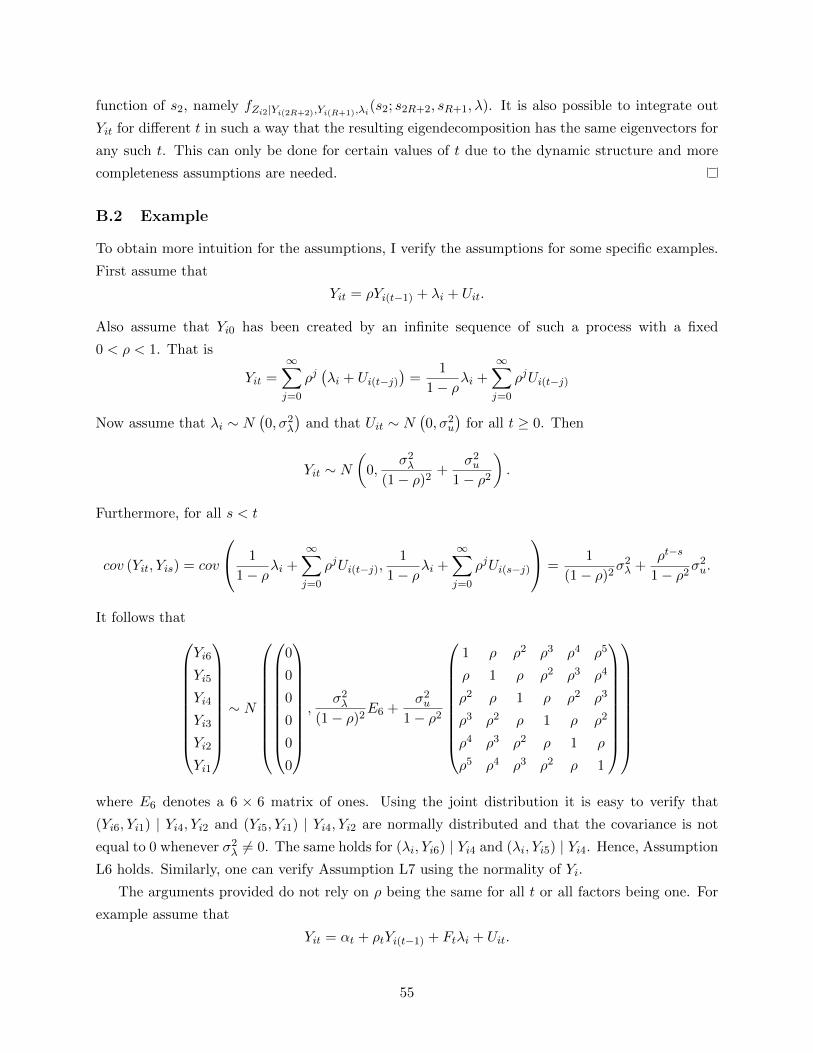
function of s2, namely fZi2|Yi(2R+2),Yi(R+1),λi(s2; s2R+2, sR+1, λ). It is also possible to integrate out

Yit for different t in such a way that the resulting eigendecomposition has the same eigenvectors for

any such t. This can only be done for certain values of t due to the dynamic structure and more

completeness assumptions are needed.

B.2 Example

To obtain more intuition for the assumptions, I verify the assumptions for some specific examples.

First assume that

Yit = ρYi(t−1) + λi + Uit.

Also assume that Yi0 has been created by an infinite sequence of such a process with a fixed

0 < ρ < 1. That is

Yit =∞∑j=0

ρj(λi + Ui(t−j)

)=

1

1− ρλi +

∞∑j=0

ρjUi(t−j)

Now assume that λi ∼ N(0, σ2

λ

)and that Uit ∼ N

(0, σ2

u

)for all t ≥ 0. Then

Yit ∼ N(

0,σ2λ

(1− ρ)2+

σ2u

1− ρ2

).

Furthermore, for all s < t

cov (Yit, Yis) = cov

1

1− ρλi +

∞∑j=0

ρjUi(t−j),1

1− ρλi +

∞∑j=0

ρjUi(s−j)

=1

(1− ρ)2σ2λ +

ρt−s

1− ρ2σ2u.

It follows that

Yi6

Yi5

Yi4

Yi3

Yi2

Yi1

∼ N

0

0

0

0

0

0

,

σ2λ

(1− ρ)2E6 +

σ2u

1− ρ2

1 ρ ρ2 ρ3 ρ4 ρ5

ρ 1 ρ ρ2 ρ3 ρ4

ρ2 ρ 1 ρ ρ2 ρ3

ρ3 ρ2 ρ 1 ρ ρ2

ρ4 ρ3 ρ2 ρ 1 ρ

ρ5 ρ4 ρ3 ρ2 ρ 1

where E6 denotes a 6 × 6 matrix of ones. Using the joint distribution it is easy to verify that

(Yi6, Yi1) | Yi4, Yi2 and (Yi5, Yi1) | Yi4, Yi2 are normally distributed and that the covariance is not

equal to 0 whenever σ2λ 6= 0. The same holds for (λi, Yi6) | Yi4 and (λi, Yi5) | Yi4. Hence, Assumption

L6 holds. Similarly, one can verify Assumption L7 using the normality of Yi.

The arguments provided do not rely on ρ being the same for all t or all factors being one. For

example assume that

Yit = αt + ρtYi(t−1) + Ftλi + Uit.

55

and

Yi0 = α0 +1

1− ρ0λi + Ui0

for some ρ ∈ (−1, 1) where Ui0 ∼ N(

0,σ20

1−ρ20

)and Uit ∼ N

(0, σ2

t

)for t ≥ 1. Then if Ft 6= 0 for all

t the assumptions can be verified in a similar way.

C Proofs and examples discrete factor models

C.1 Proof of Theorem 4

Conditional on Xi and for all mK ,m1 ∈ {1, . . . ,M} and some s define

PmK ,m1,s ≡ P(ZiK ∈ CmK , Zi1 ∈ Cm1 , ZikR+1

∈ As).

Define the matrix L1,kR+1,K as the M ×M matrix containing these probabilities for a fixed s such

that mK increases over rows while m1 increases over columns. That is

L1,kR+1,K ≡

P1,1,s P1,2,s · · · P1,M,s

P2,1,s P2,2,s · · · P2,M,s

......

. . ....

PM,1,s PM,2,s · · · PM,M,s

.

Let L1,K be the M ×M matrix containing the probabilities PmK ,m1 = P (ZiK ∈ CmK , Zi1 ∈ Cm1)

such that mK increases over rows only while m1 increases over columns. Let λ1, . . . , λM be an

ordering of all points of support of λi. Let L1,λ be the M × M matrix containing Pl,m1 =

P(Zi1 ∈ Cm1 | λi = λl

)with l increasing over rows and m1 increasing over columns. Let Lλ,K

be the matrix containing PmK ,l = P(ZiK ∈ Cm1 , λi = λl

)with l increasing over columns and mK

over rows. Let DkR+1,λ be a diagonal matrix containing P(ZikR+1

∈ As | λi = λl)

on the diagonal.

Recall that s is fixed.

As in the continuous case, it is easy to show that the assumptions and definitions imply that

L1,kR+1,KL−11,K = L1,λDkR+1,λL

−11,λ.

The eigenvectors sum to 1 because they contain conditional probabilities. Just as in Section 3, the

eigenfunctions are the same for all rotations K and any s. By Assumptions D3, D5, and full rank

of F 1, the eigenvalues are unique, when considering all K and partitions of the support of ZikR+1.

The ordering of the eigenvectors follows from the assumption that F 3 = IR×R and Assumption D5.

Therefore, all elements of L1,λ as well as DkR+1,λ and L−1K,λ are identified.

Now for all t let At,1, . . . , At,S be a partition of Yt with At,s = As for all t = 1, . . . , R. Let K =

{1, . . . , R}. Define L1,K , LK,λ, and L1,λ analogously to L1,K , LK,λ, and L1,λ but using the sets At,s

56

instead ofAt,s. It then holds that L−1K,λ = L−1

K,λ and L1,KL−1K,λ = L1,λ. The left hand side is identified,

hence the right hand side is identified for any At,s. Thus P(Yit ∈ At,s | λi = λm

)is identified for all

t = R+2, . . . , T and all s and m. Since the partition is arbitrary, P (Yit ∈ Bt | λi = λm) is identified

for all t = R+ 2, . . . , T . Similar argument yield P (Yit ∈ Bt, λi = λm) for all t = 1, . . . , R+ 1.

C.2 Example

As an illustrative example assume that Yit ∈ [0, 1], R = 2, T = 5, and S = 2. Let the points

of support of λi be {(l1, l2), (l1, h2), (h1, l2), (h1, h2)} with l1 < h1 and l2 < h2. This setup could

interpreted as each person having two skills such as cognitive and noncognitive skills. For each

skill, a person can either be of low type or of high type. Now define A1 = [0, 0.5] and A2 = (0.5, 1].

Hence C1 = [0, 0.5]× [0, 0.5], C2 = [0, 0.5]×(0.5, 1], C3 = (0.5, 1]× [0, 0.5] and C4 = (0.5, 1]×(0.5, 1].

Let Zi1 = (Yi4, Yi5) and ZK1 = (Yi1, Yi2). Let PmK ,m1 = P (ZiK ∈ CmK , Zi1 ∈ Cm1). Then

L1,K =

P1,1 P1,2 P1,3 P1,4

P2,1 P2,2 P2,3 P2,4

P3,1 P3,2 P3,3 P3,4

P4,1 P4,2 P4,3 P4,4

and L1,kR+1,K is defined similarly but contains P

(ZiK ∈ CmK , Zi1 ∈ Cm1 , ZikR+1

∈ As)

for a fixed

s. The eigenvectors are contained in L1,λ which in this case is

L1,λ =

P(Zi1 ∈ C1 | λi = λ1

)P(Zi1 ∈ C1 | λi = λ2

)P(Zi1 ∈ C1 | λi = λ3

)P(Zi1 ∈ C1 | λi = λ4

)P(Zi1 ∈ C2 | λi = λ1

)P(Zi1 ∈ C2 | λi = λ2

)P(Zi1 ∈ C2 | λi = λ3

)P(Zi1 ∈ C2 | λi = λ4

)P(Zi1 ∈ C3 | λi = λ1

)P(Zi1 ∈ C3 | λi = λ2

)P(Zi1 ∈ C3 | λi = λ3

)P(Zi1 ∈ C3 | λi = λ4

)P(Zi1 ∈ C4 | λi = λ1

)P(Zi1 ∈ C4 | λi = λ2

)P(Zi1 ∈ C4 | λi = λ3

)P(Zi1 ∈ C4 | λi = λ4

)

.

Notice that the eigenvectors sum to 1. Assumptions D5 and D6 imply that for all m = 1, 2, 3

P(Zi1 ∈ C4 | λi = λ4

)> P (Zi1 ∈ C4 | λi = λm)

and for all m = 2, 3, 4

P(Zi1 ∈ C4 | λi = λ1

)< P (Zi1 ∈ C4 | λi = λm) .

Moreover,

P (Yi4 ∈ (0.5, 1] | λi = λ2) > P (Yi4 ∈ (0.5, 1] | λi = λ3)

or equivalently

P(Zi1 ∈ C3 | λi = λ2

)+ P

(Zi1 ∈ C4 | λi = λ2

)> P

(Zi1 ∈ C3 | λi = λ3

)+ P

(Zi1 ∈ C4 | λi = λ3

).

57

To sum up, the data provides L1,kR+1,KL−11,K for all rotations K and all s. There are exactly 4

vectors with elements summing to 1, which are eigenvectors of L1,kR+1,KL−11,K for all rotations K

and all s. The vector with the smallest fourth element belongs to λ1 and the element with the

largest fourth element belongs to λ4. The other two vectors can be distinguished by the sum of

their third and fourth element: the larger sum belongs to λ2. The assumption that F 3 = IR×R can

in this case therefore be replaced with the weaker assumptions:

1. P(Zi1 ∈ C4 | λi = λ4

)> P (Zi1 ∈ C4 | λi = λm) for all m = 1, 2, 3,

2. P(Zi1 ∈ C4 | λi = λ1

)< P (Zi1 ∈ C4 | λi = λm) for all m = 2, 3, 4, and

3. P (Yi4 ∈ (0.5, 1] | λi = λ2) > P (Yi4 ∈ (0.5, 1] | λi = λ3) .

D Estimation

D.1 Fully nonparametric estimator

I first make the following three assumptions which strengthen Assumptions S5 and S8. These

assumptions can be avoided if constraints on the unknown functions are imposed, which ensure

that λi is bounded complete for Zi1.

Assumption E1. Ui1, . . . , UiT , λi are jointly independent conditional on Xi ∈ X .

Assumption E2. Zi1 is bounded complete for ZiK and ZiK is bounded complete for Zi1 for any

ordering K conditional on Xi ∈ X .

Assumption E3. λi has support on RR.

Assumptions E1 - E3 imply that λi is complete for Zi1 which follows from Theorem 2.1 in Mattner

(1993), Proposition 2.4. in D’Haultfoeuille (2011), and arguments in the proof of Lemma 1. Thus,

as discussed in Section 5.1.1, all completeness assumptions are on distributions of observables only.

As in Section 5.1.1 let Wi = (Yi, Xi), θ =(h1, . . . , hT , f1, . . . , fT , fλ, F

)and

l (θ,Wi) = log

∫ T∏t=1

ft(ht (Yit, Xit)− λ′Ft;Xi, λ)h′t (Yit, Xi,) fλ(λ;Xi)dλ.

Moreover, recall the norm

||θ||s =T∑t=1

(||ht||∞,ω1 + ||ft||∞,ω2 + ||Ft||E

)+ ||fλ||∞,ω3 .

Before, I state the smoothness assumptions let ωyl,yu(y) be a bounded weight function on [yl, yu]

such that ωyl,yu(y) > 0 for all y ∈ (yl, yu) and ωyl,yu(y) → 0 as y → yl and y → yu. Examples are

58

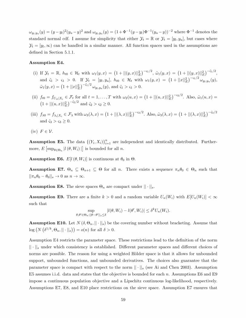
ωyl,yu(y) = (y−yl)2(yu−y)2 and ωyl,yu(y) = (1+Φ−1(y−yl)Φ−1(yu−y))−2 where Φ−1 denotes the

standard normal cdf. I assume for simplicity that either Yt = R or Yt = [yl, yu], but cases where

Yt = [yl,∞) can be handled in a similar manner. All function spaces used in the assumptions are

defined in Section 5.1.1.

Assumption E4.

(i) If Yt = R, ht0 ∈ Ht with ω1(y, x) =(1 + ||(y, x)||2E

)−ς1/2, ω1(y, x) =(1 + ||(y, x)||2E

)−ς1/2,

and ς1 > ς1 > 0. If Yt = [yl, yu], ht0 ∈ Ht with ω1(y, x) =(1 + ||x||2E

)−ς1/2 ωyl,yu(y),

ω1(y, x) =(1 + ||x||2E

)−ς1/2 ωyl,yu(y), and ς1 > ς1 > 0.

(ii) ft0 = fUit|Xi ∈ Ft for all t = 1, . . . , T with ω2(u, x) =(1 + ||(u, x)||2E

)−ς2/2. Also, ω1(u, x) =(1 + ||(u, x)||2E

)−ς2/2 and ς2 > ς2 ≥ 0.

(iii) fλ0 = fλi|Xi ∈ Fλ with ω3(λ, x) =(1 + ||(λ, x)||2E

)−ς3/2. Also, ω3(λ, x) =(1 + ||(λ, x)||2E

)−ς3/2and ς3 > ς3 ≥ 0.

(iv) F ∈ V.

Assumption E5. The data {(Yi, Xi)}ni=1 are independent and identically distributed. Further-

more, E[supθ∈Θn |l (θ,Wi) |

]is bounded for all n.

Assumption E6. E[l (θ,Wi)] is continuous at θ0 in Θ.

Assumption E7. Θn ⊆ Θn+1 ⊆ Θ for all n. There exists a sequence πnθ0 ∈ Θn such that

||πnθ0 − θ0||s → 0 as n→∞.

Assumption E8. The sieve spaces Θn are compact under || · ||s.

Assumption E9. There are a finite k > 0 and a random variable Un(Wi) with E[Un(Wi)] < ∞such that

supθ,θ′∈Θn:||θ−θ′||s≤δ

|l(θ,Wi)− l(θ′,Wi)| ≤ δkUn(Wi).

Assumption E10. Let N (δ,Θn, || · ||s) be the covering number without bracketing. Assume that

log(N(δ1/k,Θn, || · ||s

))= o(n) for all δ > 0.

Assumption E4 restricts the parameter space. These restrictions lead to the definition of the norm

|| · ||s under which consistency is established. Different parameter spaces and different choices of

norms are possible. The reason for using a weighted Holder space is that it allows for unbounded

support, unbounded functions, and unbounded derivatives. The choices also guarantee that the

parameter space is compact with respect to the norm || · ||s (see Ai and Chen 2003). Assumption

E5 assumes i.i.d. data and states that the objective is bounded for each n. Assumptions E6 and E9

impose a continuous population objective and a Lipschitz continuous log-likelihood, respectively.

Assumptions E7, E8, and E10 place restrictions on the sieve space. Assumption E7 ensures that

59

the sieve space grows as n→∞, while Assumption E10 states that the sieve space cannot grow too

fast. See Chen (2007) and references therein for choices of sieves that satisfy these assumptions.

For finite dimensional linear sieves, Assumption E10 is typically satisfied if dim(Θn)/n→ 0.

The most important aspects of the assumptions are uniqueness of the solution in the population

(identification), compactness of the parameter space, and uniform convergence over the sieves space.

As mentioned above, without Assumptions E1 - E3 one needs other conditions to ensure that the

population maximizer over the parameter space is unique. Section 5.1.1 mentions other compact

classes of functions and norms which are suitable in some applications. Uniform convergence

depends on the choice of sieves and is in general not a necessary condition. See Bierens (2012) for

an alternative approach.

I now restate Theorem 5. The theorem is a direct consequence of Theorem 3.1 in combination

with Condition 3.5M in Chen (2007). Hence, the proof is omitted.

Theorem 5. Let Assumptions E1 - E10 hold. Then

||θ − θ0||sp→ 0.

In order to implement the estimator one needs to choose basis functions as well as the length

of the sieve space. For density functions, orthogonal Hermite polynomials are a good choice (see

Gallant and Nychka (1987) and Chen (2007)). One could also use spline-wavelets as discussed by

Ai and Chen (2003). Using these basic functions, it is easy to impose conditions on the density

functions such that they are positive and integrate to 1. An alternative approach is to approximate

the square root of the density with a linear sieve. This approach has the advantage that the

functions are positive by construction. In my simulations and in the application both approaches

yield very similar results. Furthermore, the results in the application are not very sensitive to the

number of terms in the sieve space. Finally notice that when evaluating the likelihood, one has to

integrate over λ. In practice, solving the integral exactly is too time consuming. Therefore, one has

to use a numerical approximation. Possible choices are quadrature rules or Monte Carlo integration,

which are both easy to implement. The theory part assumes that the integral is evaluated exactly,

or that the approximation error is small enough relative to the sampling error in the data. In my

application and the simulations, I use Gauss Hermite quadrature rules.

D.2 Semi-parametric estimator

First, similar as in the nonparametric case, define the function spaces

Ft ≡

{ηt ∈ Λγ2,ω2

c (Ut) for some γ2 > 1 :

∫Utηt(u)du = 1 and ηt(u) ≥ 0 and S4 holds

}

60

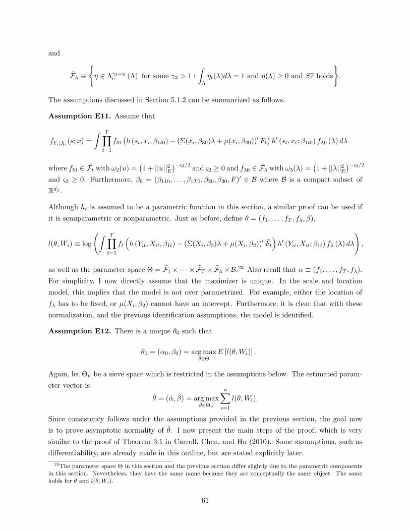
and

Fλ ≡

{η ∈ Λγ3,ω3

c (Λ) for some γ3 > 1 :

∫Ληt(λ)dλ = 1 and η(λ) ≥ 0 and S7 holds

}.

The assumptions discussed in Section 5.1.2 can be summarized as follows.

Assumption E11. Assume that

fYi|Xi(s;x) =

∫ T∏t=1

ft0(h (st, xi, β1t0)− (Σ(xi, β30)λ+ µ(xi, β20))′ Ft

)h′ (st, xt;β1t0) fλ0 (λ) dλ

where ft0 ∈ Ft with ω2(u) =(1 + ||u||2E

)−ς2/2 and ς2 ≥ 0 and fλ0 ∈ Fλ with ω3(λ) =(1 + ||λ||2E

)−ς3/2and ς3 ≥ 0. Furthermore, β0 = (β110, . . . , β1T0, β20, β30, F )′ ∈ B where B is a compact subset of

Rdβ .

Although ht is assumed to be a parametric function in this section, a similar proof can be used if

it is semiparametric or nonparametric. Just as before, define θ = (f1, . . . , fT , fλ, β),

l(θ,Wi) ≡ log

(∫ T∏t=1

ft

(h (Yit, Xit, β1t)− (Σ(Xi, β3)λ+ µ(Xi, β2))′ Ft

)h′ (Yii, Xit;β1t) fλ (λ) dλ

),

as well as the parameter space Θ = F1× · · · × FT × Fλ×B.23 Also recall that α ≡ (f1, . . . , fT , fλ).

For simplicity, I now directly assume that the maximizer is unique. In the scale and location

model, this implies that the model is not over parametrized. For example, either the location of

fλ has to be fixed, or µ(Xi, β2) cannot have an intercept. Furthermore, it is clear that with these

normalization, and the previous identification assumptions, the model is identified.

Assumption E12. There is a unique θ0 such that

θ0 = (α0, β0) = arg maxθ∈Θ

E [l(θ,Wi)] .

Again, let Θn be a sieve space which is restricted in the assumptions below. The estimated param-

eter vector is

θ = (α, β) = arg maxθ∈Θn

n∑i=1

l(θ,Wi).

Since consistency follows under the assumptions provided in the previous section, the goal now

is to prove asymptotic normality of θ. I now present the main steps of the proof, which is very

similar to the proof of Theorem 3.1 in Carroll, Chen, and Hu (2010). Some assumptions, such as

differentiability, are already made in this outline, but are stated explicitly later.

23The parameter space Θ in this section and the previous section differ slightly due to the parametric componentsin this section. Nevertheless, they have the same name because they are conceptually the same object. The sameholds for θ and l(θ,Wi).

61

I first prove that θ converges to θ at a rate faster than n−1/4 under a weaker norm || · ||2. The

norm is defined as

||v||2 ≡

√√√√E

[(dl(θ,Wi)

dθ[v]

)2]

wheredl(θ,Wi)

dθ[v] ≡ dl(θ + τv,Wi)

dτ

∣∣∣∣τ=0

.

The corresponding inner product is

〈v1, v2〉2 ≡ E[(

dl(θ,Wi)

dθ[v1]

)(dl(θ,Wi)

dθ[v2]

)].

Notice that the pathwise derivatives are linear in v. Let V denote the closure of linear space of

Θ− θ0 under the metric || · ||2. Then(V , 〈·, ·〉2

)is a Hilbert space and V = U ×Rdβ with U being

the closure of the linear span of F1×· · ·× FT ×Fλ−α0. The directional derivatives can be written

as

dl(θ,Wi)

dθ[θ − θ0] =

dl(θ,Wi)

dβ′(β − β0) +

dl(θ,Wi)

dα[α− α0]

=

(dl(θ,Wi)

dβ′− dl(θ,Wi)

dα[µ]

)(β − β0)

wheredl(θ,Wi)

dα[µ] =

(dl(θ,Wi)dα [µ1] . . . dl(θ,Wi)

dα [µdβ ])

and α− α0 = −µ(β − β0) with µ = (µ1, . . . , µdβ ). For any component k = 1, . . . , dβ define

µ∗k = arg minµk∈U

E

[(dl(θ,Wi)

dβj− dl(θ,Wi)

dα[µk]

)2].

Let µ∗ =(µ∗1, . . . , µ

∗dβ

)and

dl(θ,Wi)

dα[µ∗] =

(dl(θ,Wi)dα [µ∗1] . . . dl(θ,Wi)

dα [µ∗dβ ]).

Define the dβ × dβ matrix

(13) V ∗ = E

[(dl(θ,Wi)

dα[µ∗]

)′(dl(θ,Wi)

dα[µ∗]

)].

Now for any ζ ∈ Rdβ\{0} consider the linear functional ζ ′β. If the functional is bounded, it follows

from the Riesz Representation Theorem that there exists a vector v∗(ζ) such that for all θ ∈ V it

62

holds that ζ ′β = 〈θ, v∗(ζ)〉2. The squared norm of this functional is

supθ 6=0

|ζ ′β|2

E

[((dl(θ,Wi)dβ′ − dl(θ,Wi)

dα [µ])′β

)2] = sup

µ6=0,β 6=0

β′(ζζ ′)β

E

[((dl(θ,Wi)dβ′ − dl(θ,Wi)

dα [µ])′β

)2]

= supβ 6=0

β′(ζζ ′)β

β′V ∗β

= ζ ′(V ∗)−1ζ.

The second equality follows from the definition of V ∗ and the last equality follows by noting that the

supremum is attained at β = (V ∗)−1ζ. Hence the functional is bounded if and only if V ∗ is positive-

definite. In this case, the Riesz representer is v∗(ζ) = (v∗β((ζ)), v∗α((ζ))) where v∗β(ζ) = (V ∗)−1ζ and

v∗α = −µ∗v∗β(ζ). As implied by the Riesz Representation Theorem, it is easy to show that

||v∗(ζ)||22 = ζ ′(V ∗)−1ζ and 〈θ, v∗(ζ)〉2 = ζ ′β.

Next, it can be shown that

ζ ′(β − β0

)=⟨θ − θ0, v

∗(ζ)⟩

2=

1

n

n∑i=1

dl(θ,Wi)

dθ[v∗(ζ)] + op(n

−1/2)

and E[dl(θ,Wi)

dθ [v∗(ζ)]]

= 0. It then follows from the central limit theorem that

1√n

n∑i=1

dl(θ,Wi)

dθ[v∗(ζ)]

d→ N

(0, E

[(dl(θ,Wi)

dθ[v∗(ζ)]

)2])

.

It was previously shown that

E

[(dl(θ,Wi)

dθ[v∗(ζ)]

)2]

= ||v||22 = ζ ′(V ∗)−1ζ.

Therefore for all ζ 6= 0 we get√nζ ′(β − β0

)d→ N

(0, ζ ′(V ∗)−1ζ

)which implies by the Cramer

Wold device that√n(β − β0

)d→ N

(0, (V ∗)−1

).

I now provide conditions for these arguments to be valid. Given consistency, the following proof

focuses on a shrinking neighborhood of θ0. Therefore, define the local parameter spaces

Θ0s = {θ ∈ Θ : ||θ − θ0||s = o(1), ||θ||s ≤ c} .

and

Θ0sn = {θ ∈ Θn : ||θ − θ0||s = o(1), ||θ||s ≤ c} .

63

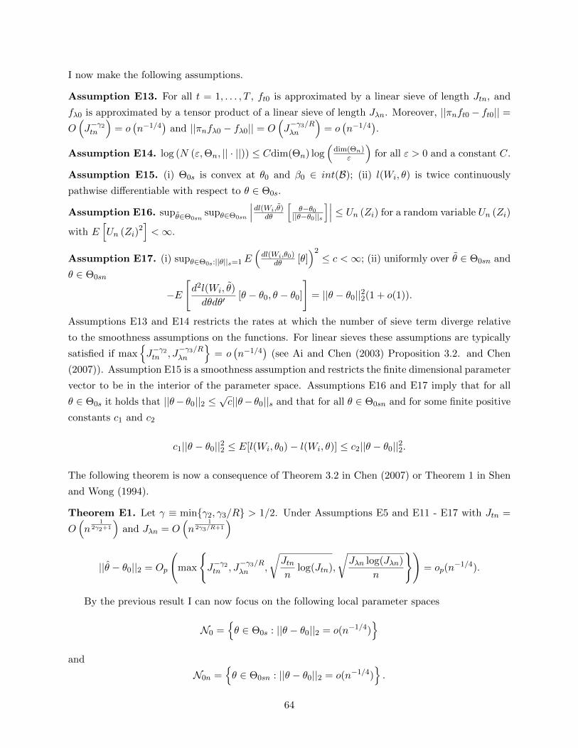
I now make the following assumptions.

Assumption E13. For all t = 1, . . . , T , ft0 is approximated by a linear sieve of length Jtn, and

fλ0 is approximated by a tensor product of a linear sieve of length Jλn. Moreover, ||πnft0 − ft0|| =O(J−γ2tn

)= o

(n−1/4

)and ||πnfλ0 − fλ0|| = O

(J−γ3/Rλn

)= o

(n−1/4

).

Assumption E14. log (N (ε,Θn, || · ||)) ≤ Cdim(Θn) log(

dim(Θn)ε

)for all ε > 0 and a constant C.

Assumption E15. (i) Θ0s is convex at θ0 and β0 ∈ int(B); (ii) l(Wi, θ) is twice continuously

pathwise differentiable with respect to θ ∈ Θ0s.

Assumption E16. supθ∈Θ0snsupθ∈Θ0sn

∣∣∣dl(Wi,θ)dθ

[θ−θ0||θ−θ0||s

]∣∣∣ ≤ Un (Zi) for a random variable Un (Zi)

with E[Un (Zi)

2]<∞.

Assumption E17. (i) supθ∈Θ0s:||θ||s=1E(dl(Wi,θ0)

dθ [θ])2≤ c <∞; (ii) uniformly over θ ∈ Θ0sn and

θ ∈ Θ0sn

−E

[d2l(Wi, θ)

dθdθ′[θ − θ0, θ − θ0]

]= ||θ − θ0||22(1 + o(1)).

Assumptions E13 and E14 restricts the rates at which the number of sieve term diverge relative

to the smoothness assumptions on the functions. For linear sieves these assumptions are typically

satisfied if max{J−γ2tn , J

−γ3/Rλn

}= o

(n−1/4

)(see Ai and Chen (2003) Proposition 3.2. and Chen

(2007)). Assumption E15 is a smoothness assumption and restricts the finite dimensional parameter

vector to be in the interior of the parameter space. Assumptions E16 and E17 imply that for all

θ ∈ Θ0s it holds that ||θ− θ0||2 ≤√c||θ− θ0||s and that for all θ ∈ Θ0sn and for some finite positive

constants c1 and c2

c1||θ − θ0||22 ≤ E[l(Wi, θ0)− l(Wi, θ)] ≤ c2||θ − θ0||22.

The following theorem is now a consequence of Theorem 3.2 in Chen (2007) or Theorem 1 in Shen

and Wong (1994).

Theorem E1. Let γ ≡ min{γ2, γ3/R} > 1/2. Under Assumptions E5 and E11 - E17 with Jtn =

O(n

12γ2+1

)and Jλn = O

(n

12γ3/R+1

)

||θ − θ0||2 = Op

(max

{J−γ2tn , J

−γ3/Rλn ,

√Jtnn

log(Jtn),

√Jλn log(Jλn)

n

})= op(n

−1/4).

By the previous result I can now focus on the following local parameter spaces

N0 ={θ ∈ Θ0s : ||θ − θ0||2 = o(n−1/4)

}and

N0n ={θ ∈ Θ0sn : ||θ − θ0||2 = o(n−1/4)

}.

64

The following assumptions are sufficient conditions for asymptotic normality of the finite dimen-

sional parameter vector β.

Assumption E18. µ∗ exists and V ∗ is positive definite.

Assumption E19. There exists v∗n ∈ Θn − πnθ0 such that ||v∗n − v∗||2 = o(1) and ||v∗n − v∗||2||θ −θ0||2 = op

(1√n

).

Assumption E20. There exists a random variable Un(Zi) with E[Un(Zi)2] <∞ and a nonnegative

measurable function q with limδ→0 q(δ) = 0 such that for all θ ∈ N0n

supθ∈N0

∣∣∣∣∣∣d2l(Wi, θ

)dθdθ′

[θ − θ0, v∗n]

∣∣∣∣∣∣ ≤ Un (Wi) q(||θ − θ0||s).

Assumption E21. Uniformly over θ ∈ N0n and θ ∈ N0

E

d2l(Wi, θ

)dθdθ′

[θ − θ0, v∗n]− d2l (Wi, θ0)

dθdθ′[θ − θ0, v

∗n]

= o

(1√n

).

Assumption E18 is a necessary assumption for√n estimation of β0. Assumption E19 ensures that

the sieve bias is negligible while Assumptions E20 and E21 control the reminder term. These as-

sumptions are standard in nonparametric maximum likelihood estimation (see for example Carroll,

Chen, and Hu (2010) or Ackerberg, Chen, and Hahn (2012)). Theorem 6 now follows.

Theorem 6. Assume that Assumptions E5 and E11 - E21 hold. Then

√n(β − β0

)d→ N

(0, (V ∗)−1

).

The proof of this theorem follows the same steps as the proof of Theorem 3.1 in Carroll, Chen,

and Hu (2010) assuming that their model is correctly specified. Hence, it is omitted.

65

E Additional tables application

Table 6: Questionnaire items used to construct teaching measures

Mathematics

Traditional We memorize formulas and procedures.

We listen to the teacher give a lecture-style presentation.

Modern We work together in small groups.

We relate what we are learning in mathematics to our daily lives.

We explain our answers.

We give explanations about what we are studying.

We decide on our own procedures for solving complex problems.

Science

Traditional We memorize science facts and principles.

We listen to the teacher give a lecture-style presentation.

We read our science textbooks and other resource materials.

Modern We work in small groups on an experiment or investigation.

We relate what we are learning in science to our daily lives.

We design or plan an experiment or investigation.

We make observations and describe what we see.

Table 7: Marginal effects teaching practice for girls

Math scores Science scores

Traditional Modern Traditional Modern

Linear fixed effects 0.033 -0.004 0.067** 0.003

Parametric - one factor - Ft = 1 0.034*** -0.004 0.069*** 0.004

Parametric - one factor 0.075*** -0.011 0.122*** -0.033**

Parametric - two factor 0.281*** -0.238*** -0.140** 0.315***

Semiparametric - two factors 0.279*** -0.260*** -0.131* 0.257***

66

References

Ackerberg, D., X. Chen, and J. Hahn (2012). A practical asymptotic variance estimator for two-step

semiparametric estimators. The Review of Economics and Statistics 94 (2), 481–498.

Ahn, S., Y. Lee, and P. Schmidt (2001). GMM estimation of linear panel data models with time-

varying individual effects. Journal of Econometrics 101 (2), 219–255.

Ahn, S., Y. Lee, and P. Schmidt (2010). Panel data models with multiple time-varying individual

effects. Working paper.

Ai, C. and X. Chen (2003). Efficient estimation of modelswith conditional moment restrictions

containing unknown functions. Econometrica 71 (6), 1795–1843.

Altonji, J. and R. Matzkin (2005). Cross section and panel data estimators for nonseparable models

with endogenous regressors. Econometrica 73 (4), 1053–1102.

Andrews, D. (2005). Cross-section regression with common shocks. Econometrica 73 (5), 1551–1585.

Arellano, M. and S. Bonhomme (2011). Nonlinear panel data analysis. Annual Review of Eco-

nomics 3, 395–424.

Arellano, M. and S. Bonhomme (2012). Identifying distributional characteristics in random coeffi-

cients panel data models. Review of Economic Studies 79 (3), 987–1020.

Aucejo, E. (2011). Assessing the role of teacher-student interactions. Working paper.

Bai, J. (2003). Factor models of large dimensions. Econometrica 71 (1), 135–171.

Bai, J. (2009). Panel data models with interactive fixed effects. Econometrica 77 (4), 1229–1279.

Bai, J. (2012). Fixed-effects dynamic panel models, a factor analytical method. Econometrica,

forthcoming .

Bai, J. and S. Ng (2002). Determining the number of factors in approximate factor models. Econo-

metrica 70 (1), 191–221.

Bai, J. and S. Ng (2011). Principal components estimation and identification of the factors. Working

paper.

67

Bester, A. and C. Hansen (2009). Identification of marginal effects in a nonparametric correlated

random effects model. Journal of Business and Economic Statistics 27 (2), 235–250.

Bierens, H. (2012). Consistency and asymptotic normality of sieve estimators under weak and

verifiable conditions. Working paper.

Bietenbeck, J. (2011). Teaching practices and student achievement: Evidence from TIMSS. Working

paper.

Bonhomme, S. and J.-M. Robin (2008). Consistent noisy independent component analysis. Journal

of Econometrics 149 (1), 12–25.

Canay, I., A. Santos, and A. Shaikh (2012). On the testability of identification in some nonpara-

metric models with endogeneity. Working paper.

Carneiro, P., K. T. Hansen, and J. J. Heckman (2003). Estimating distributions of treatment effects

with an application to the returns to schooling and measurement of the effects of uncertainty on

college choice. International economic review 44 (2), 361–422.

Carroll, R. J., X. Chen, and Y. Hu (2010). Identification and estimation of nonlinear models using

two samples with nonclassical measurement errors. Journal of Nonparametric Statistics 22 (4),

379–399.

Chamberlain, G. (2010). Binary response models for panel data: Identification and information.

Econometrica 78 (1), 159–168.

Chen, X. (2007). Large sample sieve estimation of semi-nonparametric models. In J. Heckman and

E. Leamer (Eds.), Handbook of Econometrics, Volume 6 of Handbook of Econometrics, Chap-

ter 76, pp. 5550–5623. Elsevier.

Chen, X., E. Tamer, and A. Torgovitsky (2011). Sensitivity analysis in semiparametric likelihood

models. Working paper.

Chernozhukov, V., I. Fernandez-Val, J. Hahn, and W. Newey (2012). Average and quantile effects

in nonseparable panel models. Econometrica, forthcoming .

Clotfelter, C. T., H. F. Ladd, and J. L. Vigdor (2010). Teacher credentials and student achieve-

ment in high school: A cross-subject analysis with student fixed effects. Journal of Human

Resources 45 (3), 655–681.

68

Cunha, F. and J. J. Heckman (2008). Formulating, identifying and estimating the technology of

cognitive and noncognitive skill formation. Journal of Human Resources 43 (4), 738–782.

Cunha, F., J. J. Heckman, and S. M. Schennach (2010). Estimating the technology of cognitive

and noncognitive skill formation. Econometrica 78 (3), 883–931.

Dee, T. S. (2007). Teachers and the gender gaps in student achievement. Journal of Human

Resources 42 (03), 528–554.

Delaigle, A., P. Hall, and A. Meister (2008). On deconvolution with repeated measurements. The

Annals of Statistics 36 (2), 665 – 685.

D’Haultfoeuille, X. (2011). On the completeness condition in nonparametric instrumental problems.

Econometric Theory 27 (3), 460–471.

Dudley, R. and W. Philipp (1983). Invariance principles for sums of banach space valued ran-

dom elements and empirical processes. Zeitschrift fur Wahrscheinlichkeitstheorie und verwandte

Gebiete 62, 509–552.

Evdokimov, K. (2010). Identification and estimation of a nonparametric panel data model with

unobserved heterogeneity. Working paper.

Evdokimov, K. (2011). Nonparametric identification of a nonlinear panel model with application

to duration analysis with multiple spells. Working paper.

Fan, J. (1991). On the optimal rates of convergence for nonparametric deconvolution problems.

The Annals of Statistics 19 (3), 1257–1272.

Gallant, A. R. and D. W. Nychka (1987). Semi-nonparametric maximum likelihood estimation.

Econometrica 55 (2), 363–90.

Graham, B. and J. Powell (2012). Identification and estimation of average partial effects in “irreg-

ular” correlated random coefficient panel data models. Econometrica 80 (5), 2105–2152.

Heckman, J. J., J. Stixrud, and S. Urzua (2006). The effects of cognitive and noncognitive abilities

on labor market outcomes and social behavior. Journal of Labor Economics 24 (3), 411–482.

Hoderlein, S. and H. White (2012). Nonparametric identification in nonseparable panel data models

with generalized fixed effects. Journal of Econometrics 168 (2), 300–314.

69

Holtz-Eakin, D., W. Newey, and H. S. Rosen (1988). Estimating vector autoregressions with panel

data. Econometrica 56 (6), 1371–1395.

Honore, B. E. and E. Tamer (2006). Bounds on parameters in panel dynamic discrete choice models.

Econometrica 74 (3), 611–629.

Hu, Y. (2008). Identification and estimation of nonlinear models with misclassification error using

instrumental variables: A general solution. Journal of Econometrics 144 (1), 27–61.

Hu, Y. and S. M. Schennach (2008). Instrumental variable treatment of nonclassical measurement

error models. Econometrica 76 (1), 195–216.

Hu, Y. and M. Shum (2012). Nonparametric identification of dynamic models with unobserved

state variables. Journal of Econometrics, forthcoming .

Huang, X. (2010). Nonparametric estimation in large panels with cross sectional dependence.

Working paper.

Lavy, V. (2011). What makes an effective teacher? quasi-experimental evidence. Working paper.

Lui, X. and Y. Shao (2003). Asymptotics for likelihood ratio tests under loss of identifiability. The

Annals of Statistics 31 (3), 807–832.

Mattner, L. (1993). Some incomplete but boundedly complete location families. The Annals of

Statistics 21 (4), 2158–2162.

Moon, H. R. and M. Weidner (2010). Linear regression for panel with unknown number of factors

as interactive fixed effects. Working paper.

Newey, W. and J. Powell (2003). Instrumental variable estimation of nonparametric models. Econo-

metrica 71 (5), 1565–1578.

Newey, W. K. and D. McFadden (1986). Large sample estimation and hypothesis testing. In

R. F. Engle and D. McFadden (Eds.), Handbook of Econometrics, Volume 4 of Handbook of

Econometrics, Chapter 36, pp. 2111–2245. Elsevier.

Pesaran, M. H. (2006). Estimation and inference in large heterogeneous panels with a multifactor

error structure. Econometrica 74, 967–1012.

Sasaki, Y. (2012). Heterogeneity and selection in dynamic panel data. Working paper.

70

Shen, X. and H. Wong (1994). Convergence rate of sieve estimates. The Annals of Statistics 22 (2),

580–615.

Shiu, J.-L. and Y. Hu (2011). Identification and estimation of nonlinear dynamic panel data models

with unobserved covariates. Working paper.

Su, L. and S. Jin (2012). Sieve estimation of panel data models with cross section dependence.

Journal of Econometrics 169 (1), 34–47.

Weidner, M. (2011). Semiparametric estimation of nonlinear panel data models with generalized

random effects. Working paper.

Williams, B. (2011). A measurement model with discrete measurements and continuous latent

variables. Working paper.

Williams, B., J. Heckman, and S. Schennach (2010). Nonparametric factor score regression with

an application to the technology of skill formation. Working paper.

Zemelman, S., H. Daniels, and A. Hyde (2005). Best practice: today’s standards for teaching and

learning in America’s schools. Heinemann.

71