Panel Data Models with Interactive Fixed Effects and

Multiple Structural Breaks

Degui Li∗

University of York

Junhui Qian†

Shanghai Jiao Tong University

Liangjun Su‡

Singapore Management University

July 26, 2014

Abstract

In this paper we consider estimation and inference of common structural breaks in panel

data models with interactive fixed effects which are unobservable. We introduce a penalized

principal component (PPC) estimation procedure with adaptive group fused LASSO to detect

the multiple structural breaks in the models. Under some mild conditions, we show that with

probability approaching one our method can correctly determine the unknown number of breaks

and consistently estimate the common break dates. Furthermore, to improve the convergence

rates, we estimate the regression coefficients through the post-LASSO method and establish the

asymptotic distribution theory for the resulting estimators. The developed methodology and

theory are also applicable to the case of dynamic panel data. We propose a data-driven method

to determine the tuning parameter involved in the PPC estimation procedure. The Monte Carlo

simulation results demonstrate that the proposed method works well in finite samples with low

false detection probability when there is no structural break and high probability of correctly

estimating the break numbers when the structural breaks exist.

JEL subject classifications: C33, C13.

∗Department of Mathematics, University of York, Heslington, YO10 5DD, UK. Email: degui.li@york.ac.uk.†Antai College of Economics and Management, Shanghai Jiao Tong University, Shanghai 200052, China. Email:

jhqian@sjtu.edu.cn.‡School of Economics, Singapore Management University, Singapore 178903, Singapore. Email: ljsu@smu.edu.sg.

1

Keywords: Change point, interactive fixed effects, LASSO, panel data, penalized estimation,

principal component analysis.

1 Introduction

As the availability of panel or longitudinal data increases in the last few decades, panel data studies

have become increasingly popular among a wide group of statisticians and econometricians. Analysis

of panel data sets has various advantages over that of purely time series or cross-sectional data sets,

and the most important advantage is probably that the panel data provide researchers with more

flexibility to model dynamics in cross-sectional units and uncover possible structural changes over

time. In recent years, there has been a growing literature on the estimation and test of structural

breaks in panel data models as structural breaks are quite common in many areas such as economics

and finance, and may occur for various reasons. For example, the global financial crisis and the

ensuing government regulation overhaul may fundamentally change how risks are priced in the finan-

cial markets. If such structural changes are ignored in the modelling, subsequent statistical analyses

based on financial data may lead to incorrect inferences or misleading predictions.

Generally speaking, most of the existing literature on estimating panel structural breaks falls into

two categories depending on whether the parameters of interest are allowed to be heterogenous across

subjects or not. The first category focuses on homogenous panel data models (c.f., De Watcher and

Tzavalis, 2012; and Qian and Su, 2014) and the second category considers estimation and inference

of common breaks in heterogenous panel data models (c.f., Bai, 2010; Kim, 2011; Baltagi et al.,

2013). Despite the vast literature on multiple structural breaks in the time series framework (c.f.,

Csorgo and Horvath, 1997; Bai and Perron, 1998; Qu and Perron, 2007; Harchaoui and Levy-Leduc,

2010; and Qian and Su, 2013), most of the existing work on panel structural breaks focuses on the

estimation and inference of a single structural break in panel data models. The only exception is

the paper by Qian and Su (2014) which considers shrinkage estimation of common breaks in panel

data models. However, Qian and Su’s (2014) modelling framework does not allow the existence of

cross sectional dependence, which limits the applicability of their techniques as the cross sectional

dependence commonly exists in many panel data sets nowadays (such as the panel climate data).

In this paper, we aim to estimate multiple structural breaks in panel data models with cross-

sectional dependence which is described through the unobservable interactive fixed effects. Such

cross-sectional dependence structure in analysis of panel data has received increasing interest in

2

recent years (c.f., Pesaran, 2006; Bai, 2009; Moon and Weidner, 2013; Bai and Li, 2014). However,

to the best of our knowledge, there is virtually no work on estimating multiple structural breaks in

panel data models with interactive fixed effects and possible dynamic structure (such as the dynamic

autoregressive panel data models). As in Qian and Su (2014), we apply the shrinkage idea through

the adaptive group fused LASSO (AGF LASSO) to estimate the multiple structural break dates.

Nevertheless, the existence of the unobservable interactive fixed effects in our model makes the

estimation techniques and the development of the asymptotic theory much more involved than those

in Qian and Su (2014). In Section 2 below, we introduce a novel penalized principal component (PPC)

estimation procedure via AGF LASSO to estimate both the regression coefficients and the factor

loadings. Similar to the sparsity result in the high-dimensional variable selection literature (c.f., Fan

and Li, 2001, 2006), we establish the consistency for the detection of the multiple structural breaks,

which indicates that both the number of breaks and the break dates can be consistently estimated.

Furthermore, to improve the convergence rates, we also estimate the regression coefficients through

the post-LASSO method and then establish the asymptotic distribution theory of the resulting

estimators, which generalizes the results in Bai (2009) and Moon and Weidner (2013) where there

is no structural break. The simulation studies show that the proposed PPC method has an high

probability of correctly estimating the number of breaks when the structural breaks exist in panel

data models, and a low probability of false detection when there is no structural break.

The rest of the paper is organized as follows. Section 2 introduces the model and the PPC

estimation method. Section 3 gives the asymptotic properties for the PPC estimator as well as the

post-LASSO estimator. Section 4 reports the Monte Carlo simulation results. Section 5 concludes

the paper. Appendices A and B give the assumptions and the proofs of the asymptotic results,

respectively. Some technical lemmas as well as their proofs are collected in Appendix C of the

supplemental document. Throughout the paper, we adopt the following notations. For an m×n real

matrix A (or vector) we denote its transpose as A′, its Frobenius norm as ‖A‖ (≡ [tr(AA′)]1/2), its

spectral norm as ‖A‖sp (≡ [µmax (AA′)]1/2

), and its Moore-Penrose generalized inverse as A+. Let

PA = A (A′A)+A′ and MA = Im − PA, where Im is an m × m identity matrix with m being

the number of rows for A. When A is symmetric, we use µr(A) to denote its rth largest eigenvalue

by counting multiple eigenvalues multiple times, and µmax(A) and µmin(A) to denote the largest

and smallest eigenvalues of A, respectively. Let vec(A) be the vectorization of the matrix A and let

Tr(A) be the trace of a square matrix A. Let 0 denote a null matrix or vector whose size may change

from line to line, and 1· be the usual indicator function. The operatorP→ denotes convergence

in probability,D→ convergence in distribution, and plim probability limit. We use (N, T ) → ∞ to

denote that both N and T pass to infinity jointly.

3

2 Model and estimation method

In this section, we first introduce a panel data model with interactive fixed effects and an unknown

number of structural breaks, and then propose the PPC estimation method for the model.

2.1 The model

Let Yit be the dependent variable for subject i measured at time t where i = 1, · · · , N, and t =

1, · · · , T . We consider the following panel data model with interactive fixed effects

Yit = β′tXit + λ′ift + εit, i = 1, · · · , N, t = 1, · · · , T, (2.1)

where Xit is a p× 1 vector of explanatory variables, βt is a p× 1 vector of unknown slope coefficients

which may change over time, λi and ft denote an R0 × 1 vector of unobservable factor loadings and

common factors, respectively, both of which may be correlated with Xit, and εit is the idiosyncratic

error term. Throughout the paper, we denote the true value of a parameter vector with a superscript

0. For instance, β0t , λ

0i and f 0

t denote the true values of βt, λi and ft, respectively. We allow the

regression coefficients to vary across the time and model (2.1) thus includes the classical linear panel

data models with interactive fixed effects (c.f., Pesaran, 2006; Bai, 2009; Moon and Weidner, 2013)

as a special case. As in these papers, we also assume that both the cross-sectional size N and the

time series length T pass to infinity, which is called as “large dimensional panel” in the literature.

In this paper we assume that the true regression coefficientsβ0

1, · · · , β0T

exhibit certain sparse

nature such that the total number of distinct vectors in the set is given by m0 + 1, which is unknown

but typically much smaller than the time series length T. In fact, following the literature we assume

that m0 is a fixed nonnegative integer. More specifically, we let

β0t = α0

j for t = T 0j−1, · · · , T 0

j − 1 with j = 1, · · · ,m0 + 1,

where we adopt the convention that T 00 = 1 and T 0

m0+1 = T + 1. The indices T 0j , j = 1, · · · ,m0,

indicate that there are m0 unobserved break points/dates and the number m0 + 1 denotes the total

number of regimes. We are interested in estimating the unknown number of the structural breaks, the

unobservable break dates and the regression coefficients in different regimes. Let β = (β′1, · · · , β′T )′,

αm = (α′1, · · · , α′m+1)′, Λ =(λ1, λ2, · · · , λN

)′, F =

(f1, f2, · · · , fT

)′, and Tm = (T1, · · · , Tm) .

Throughout the paper, we use m0, α0m0 =

(α0′

1 , · · · , α0′m0+1

)′and T 0

m0 =(T 0

1 , · · · , T 0m0

)to denote

the true number of structural breaks, the true vector of regression coefficients, and the set of true

break dates, respectively.

4

2.2 PPC estimation procedure

We next consider the so-called PPC estimation of the unknown components(β0,Λ0,F 0

), where

β0 =(β0′

1 , β0′2 , · · · , β0′

T

)′, Λ0 =

(λ0

1, λ02, · · · , λ0

N

)′and F 0 =

(f 0

1 , f02 , · · · , f 0

T

)′. Let Yt =

(Y1t, · · · , YNt

)′and Xt =

(X1t, · · · , XNt

)′. To apply the PPC method, we define the objective function through

QNT,γ(β,Λ,F

)=

1

NT

N∑i=1

T∑t=1

(Yit −X ′itβt − λ′ift

)2+γ

T

T∑t=2

wt∥∥βt − βt−1

∥∥ , (2.2)

which can be written as

1

NT

T∑t=1

(Yt −Xtβt −Λft)′ (Yt −Xtβt −Λft) +

γ

T

T∑t=2

wt∥∥βt − βt−1

∥∥ ,where γ ≡ γNT > 0 is a tuning parameter and wt is a data-driven weight defined by

wt =∥∥βt − βt−1

∥∥−κ, t = 2, ..., T, (2.3)

βt, t = 1, · · · , T , are the preliminary estimates of the regression coefficients βt, and κ is a user-

specified positive constant that usually takes value 2 in the literature. In this paper, the preliminary

estimationβt, t = 1, · · · , T

is constructed to minimize the first term of the above objective function

in (2.2) by ignoring the penalization device.

By concentrating F out in the first term of the objective function (2.2), we can readily obtain

the following objective function

QNT,γ (β,Λ) = QNT (β,Λ) +γ

T

T∑t=2

wt∥∥βt − βt−1

∥∥ , (2.4)

where

QNT (β,Λ) =1

NT

T∑t=1

(Yt −Xtβt)′MΛ (Yt −Xtβt) .

Following Moon and Weidner (2013), we can further concentrate Λ out in (2.4) and obtain the

objective function

QNT,γ (β) = QNT (β) +γ

T

T∑t=2

wt∥∥βt − βt−1

∥∥ , (2.5)

where

QNT (β) =1

N

N∑r=R0+1

µr[1

T

T∑t=1

(Yt −Xtβt) (Yt −Xtβt)′].

5

The implementation of the PPC estimation procedure and the establishment of its asymptotic the-

ory in this paper will be based on the minimization of the objective functions in (2.5) and (2.4),

respectively.

It can be seen that the penalization device in the above objective functions is closely related to

the literature on the adaptive LASSO (Zou, 2006), the group LASSO (Yuan and Lin, 2006), and the

fused LASSO (Tibshirani et al., 2005; Rinaldo, 2009). The use of the Frobenius norm ‖·‖ for the

vector difference βt − βt−1 generalizes the fused LASSO to the group fused LASSO; and the use of

the adaptive weights wt makes the LASSO procedure adaptive. For this reason, we can call our

penalized estimation procedure as an adaptive group fused LASSO (AGF LASSO) procedure.

Following Bai and Ng’s (2002) principal component method under the identification restrictions

that Λ′Λ/N = IR0 and F ′F is a diagonal matrix, the minimizers to the objective function defined

in (2.4), β =(β′1, · · · , β

′T

)′and Λ satisfy that

β = arg minβQNT,γ(β, Λ), (2.6)

and [ 1

NT

T∑t=1

(Yt −Xtβt

)(Yt −Xtβt

)′]Λ = ΛV NT (2.7)

where V NT is a diagonal matrix consisting of the R0 largest eigenvalues of the matrix in the square

bracket arranged in descending order. Furthermore, the common factor F 0 can be estimated by

F = (f1, f2, · · · , fT )′ with ft = N−1Λ′(Yt −Xtβt). (2.8)

An iterative algorithm based on (2.6) and (2.7) can be implemented in practice to estimate β0 and

Λ0. Note that the above calculations are different from those in the existing literature such as Bai

(2009), Lu and Su (2013), and Su (2014) by switching the role of Λ and F , because the regression

coefficients are heterogeneous over the time.

Given βt, the set of estimated break dates are given by Tm = (T1, · · · , Tm) where 2 ≤ T1 <

· · · < Tm ≤ T such that ‖βt − βt−1‖ 6= 0 at t = Tj for j = 1, · · · , m. The set Tm divides the time

interval [1, T ] into m + 1 regimes such that the parameter estimates remain constant within each

regime. Notice that if Tm = T, the last break occurs at the end of the sample and the (m+1)th regime

has only one time series observation for each cross-sectional unit. Let T0 = 1 and Tm+1 = T + 1.

Define αj = αj(Tm) = βTj−1as the estimate of α0

j for j = 1, · · · , m + 1. In the sequel, we usually

suppress the dependence of αj on Tm (or the tuning parameter γ) unless necessary. For example, we

let αm =(α′1, α

′2, · · · , α′m+1

)′to denote αm(Tm) =

[α1(Tm)′, α2(Tm)′, · · · , αm+1(Tm)′

]′.

6

3 Asymptotic properties

In this section, we give the large sample theory including the consistency of the proposed PPC

estimator and the limiting distribution of the post-LASSO estimator.

3.1 Consistency of the PPC estimator

We start with the consistency result of the PPC estimator β with convergence rates.

Theorem 3.1 Suppose that Assumptions 1 and 2(i) in Appendix A holds. Then we have (i) T−1∥∥β−

β0∥∥2

= OP

(δ−2NT

), and (ii) ‖βt − β0

t‖ = OP

(δ−1NT

), where δNT = min(

√T ,√N).

Theorems 3.1 (i) and (ii) establish the preliminary mean square and point-wise convergence rates

of βt, respectively, which is a very general result by allowing the existence of multiple jumps

in the regression coefficients. As the regression coefficients vary a lot over a time span, there is

less observational information available for the estimation of each regression coefficient (compared

with the model without any structural break), which would in turn affect the estimation accuracy

of the factor loading matrix and convergence rates for the parameters. Hence, it is not surprising

that we have the root-min(N, T ) convergence rate for the PPC estimator βt, which is slower than the

optimal root-NT rate (after bias correction) obtained in the case of no change point for the regression

coefficients (c.f., Bai, 2009; Moon and Weidner, 2013). If we assume further that N ∼ T , the above

convergence rates would become (i) T−1∥∥β − β0

∥∥2= OP (N−1) and (ii) ‖βt − β0

t‖ = OP

(N−1/2

).

Recall that T 0m0 =

T 0

1 , ..., T0m0

denotes the set of break dates and let T c = 2, ..., T \T 0

m0 . Let

θ01 = β0

1, θ1 = β1, θ0t = β0

t −β0t−1 and θt = βt− βt−1 for t = 2, ..., T. The following theorem establishes

the detection consistency, which is analogous to the sparsity result in the high-dimensional variable

selection literature.

Theorem 3.2 Suppose that Assumptions 1 and 2(i)-(ii) in Appendix A hold. Then

P(∥∥θt∥∥ = 0 for all t ∈ T c

)→ 1 as (N, T )→∞.

Theorem 3.2 shows that with probability approaching one (w.p.a.1), all the zero vectors inθ0t

must be estimated as exactly zero, which is a well-known sparsity result in the high-dimensional

variable selection literature (c.f., Fan and Li, 2006). On the other hand, by Theorem 3.1(ii), we know

that the estimates of the nonzero vectors inθ0t

are consistent by noting that βt− βt−1 consistently

estimates θ0t = β0

t − β0t−1. A combination of Theorems 3.1 and 3.2 implies that the AGF LASSO has

the ability to identify the true regression model with the correct number of structural breaks and

the correct break dates, which is stated in the following corollary.

7

Corollary 3.3 Suppose that Assumptions 1 and 2 in Appendix A hold. Then (i)

lim(N,T )→∞

P(m = m0

)= 1,

and (ii)

lim(N,T )→∞

P(T1 = T 01 , ..., Tm0 = T 0

m0) = 1.

3.2 Post-LASSO estimates

We next introduce the post-LASSO estimation of the regression coefficients, which can improve the

convergence rate of the PPC estimation given in Theorem 3.1. For any p(m+ 1)-dimensional vector

αm =(α′1, · · · , α′m+1

)′and Tm = T1, · · · , Tm with 1 < T1 < · · · < Tm ≤ T, we define the objective

function by

QNT(αm,Λ,F ; Tm

)=

1

NT

m+1∑j=1

Tj−1∑t=Tj−1

N∑i=1

(Yit −X ′itαj − λ′ift

)2=

1

NT

m+1∑j=1

Tj−1∑t=Tj−1

(Yt −Xtαj −Λft)′ (Yt −Xtαj −Λft) . (3.1)

By concentrating F out in the above objective function, we can readily obtain the following profile

post-LASSO objective function

QNT

(α,Λ; Tm

)=

1

NT

m+1∑j=1

Tj−1∑t=Tj−1

(Yt −Xtαj

)′MΛ

(Yt −Xtαj

). (3.2)

Let αm (Tm) =[α1(Tm)′, · · · , αm+1(Tm)′

]′and Λ (Tm) =

[λ1(Tm), · · · , λN(Tm)

]′denote the minimiz-

ers of the objective function defined in (3.2) for given Tm. By setting Tm as Tm = (T1, · · · , Tm), the

set of the estimated break dates constructed in Section 2.2, we obtain the post-LASSO estimate

αm ≡ αm(Tm) and Λ ≡ Λ(Tm).

We next study the asymptotic distribution of the post-LASSO estimate. Corollary 3.3 above

implies that w.p.a.1 m = m0 and Tj = T 0j for j = 1, ...,m0. Hence, it follows that αm is asymptotically

equivalent to the infeasible estimator αm0(Tm0) which is obtained only if one knows the set Tm0 of

the true break dates. Let

BNT (1) =[BNT,1(1)′, · · · , BNT,m0+1(1)′

]′and

BNT (2) =[BNT,1(2, 1)′ −BNT,1(2, 2)′, · · · , BNT,m0+1(2, 1)′ −BNT,m0+1(2, 2)′

]′,

8

where

BNT,j(1) =1

N2T 2

T 0j −1∑

t=T 0j−1

X ′tM Λm0εε′Λm0

( 1

NΛ0′Λm0

)+( 1

TF 0′F 0

)+f 0t ,

BNT,j(2, 1) =1

NT

T 0j −1∑

t=T 0j−1

X ′tΛ0( 1

NΛ0′Λ0

)+( 1

TF 0′F 0

)+[ 1

NT

T∑s=1

f 0s ε′sεt],

BNT,j(2, 2) =1

NT

T 0j −1∑

t=T 0j−1

X ′tΛ0( 1

NΛ0′Λ0

)+( 1

TF 0′F 0

)+[ 1

NT

T∑s=1

f 0t ε′sε∗t

],

and ε∗t = 1T

∑Ts=1 χstεs with χst = f 0′

s

(1TF 0′F 0

)+f 0t , ε = (ε1, · · · , εT ) with εt =

(ε1t, · · · , εNt

)′. Define

BNT = Ω+0

[BNT (1) +BNT (2)−BNT (3)

],

where Ω0 and BNT (3) are defined in Assumption 3 (iv) in Appendix A.

Theorem 3.4 Suppose that Assumptions 1–3 in Appendix A hold. Then conditional on m = m0,

we have √NT

(αm −α0 +BNT

) D−→ N(0,Ω+

0 Ω1Ω+0

),

where Ω0 and Ω1 are defined in Assumption 3 (iv) in Appendix A.

We can show that the above asymptotic bias termBNT would not affect the root-NT convergence

rate for the post-LASSO estimation, and we thus call it as the “second-order” asymptotic bias term.

Despite the use of different notations and proof strategies, Ω+0BNT (1) and Ω+

0BNT (2) correspond

to the terms −C and −B in Bai (2009) or −W−1B3 and −W−1B2 in Moon and Weidner (2013),

respectively. Like the term −W−1B1 in Moon and Weidner (2013), Ω+0BNT (3) arises here because

we allow the regressor vector Xit to contain lagged dependent variable (e.g., Yi,t−1) and it is vanishing

under Bai’s (2009) conditions A-E that include the independence between εit and (Xjs, λ0j , f

0s ) for

all i, t, j, s and thus rule out dynamics in the regression equation. As Bai (2009) remarks, in the

absence of both serial/cross-sectional correlations and heteroskedasticity and under his Assumption

D, all of these three bias terms are asymptotically negligible. In the general case, the bias terms of

the post-LASSO estimates can be removed by constructing a bias-corrected estimate. Following Bai

(2009) in the case of static panels or Moon and Weidner (2013) and Su (2013) in the case of dynamic

panels, one can easily construct a bias corrected version of our post LASSO estimate. We omit the

details as the extension is quite straightforward.

9

Note that the above theorem holds without requiring that N and T diverge to infinity at the

same speed and the latter condition was assumed in both Bai (2009) and Moon and Weidner (2013).

For the easiness of presentation, we do assume that T 0j − T 0

j−1 ∝ T in Assumption 3(ii) in Appendix

A, which implies that each regime specific regression coefficient vector α0j (j = 1, ...,m0 + 1) can be

estimated at the usual√NT -rate after possible bias correction. Apparently, it is possible to weaken

this last assumption to T 0j −T 0

j−1 →∞ and then we can anticipate that αj (Tm)’s would have different

convergence rates to their true values for j = 1, · · · ,m0 + 1.

4 Monte Carlo simulation

In this section we first introduce the choice of tuning parameter γ in the PPC estimation procedure

and then conduct a set of Monte Carlo experiments to evaluate the finite sample performance of the

proposed method.

4.1 Choice of the tuning parameter

We next discuss the choice of the tuning parameter γ in the PPC estimation procedure, which is an

important issue when the penalized methodology is used in practice. Let

αmγ = αmγ (Tmγ ) =[α1(Tmγ )′, · · · , αmγ+1(Tmγ )′

]′denote the set of post-LASSO estimates of the regression coefficients based on the break dates in

Tmγ = Tmγ (γ), where we make the dependence of various estimates on λ explicitly. Let σ2(Tmγ ) =

QNT

(αmγ , Λ, F ; Tmγ

), where F is defined similar to F in (2.8) with Λ and βt replaced by Λ and

αj(Tmγ ) when Tj−1 ≤ t ≤ Tj − 1. We then propose to select the tuning parameter γ by minimizing

the following information criterion:

IC (γ) = log[σ2(Tmγ )

]+ ρNTp

(mγ + 1

),

where ρNT is pre-determined such that ρNT → 0 and ρNT δ2NT → ∞. In the following simulation,

we choose ρNT = c log(NT )/min(N, T ) with c being a positive constant, which can satisfy the two

restrictions. More specifically, we find a tuning parameter γmax that would yield zero break in every

data generating process (DGP) and a γmin that would yield many breaks. We then search for the

optimal tuning parameter on the 40 evenly-distributed logarithmic grids in the interval [γmin, γmax].

The positive constant is set to be c = 1/20, however, it is found in separate simulations that the

10

performance of the method is not sensitive to the choice of c, especially when N or T is large. The

simulation results below will show that such a selection method for the tuning parameter performs

reasonably well in the finite sample case.

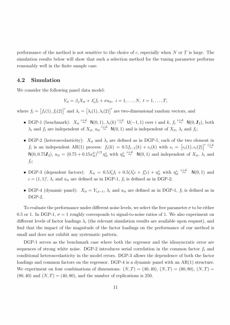
4.2 Simulation

We consider the following panel data model:

Yit = βtXit + λ′ift + σuit, i = 1, . . . , N, t = 1, . . . , T,

where ft =[ft(1), ft(2)

]′and λi =

[λi(1), λi(2)

]′are two-dimensional random vectors, and

• DGP-1 (benchmark): Xiti.i.d.∼ N(0, 1), λi(k)

i.i.d.∼ U(−1, 1) over i and k, fti.i.d.∼ N(0, I2), both

λi and ft are independent of Xit, uiti.i.d.∼ N(0, 1) and is independent of Xit, λi and ft;

• DGP-2 (heteroscedasticity): Xit and λi are defined as in DGP-1, each of the two element in

ft is an independent AR(1) process: ft(k) = 0.5ft−1(k) + εt(k) with εt =[εt(1), εt(2)

]′ i.i.d.∼N(0, 0.75I2), uit = (0.75 + 0.15x2

it)1/2η∗it with η∗it

i.i.d.∼ N(0, 1) and independent of Xit, λi and

ft;

• DGP-3 (dependent factors): Xit = 0.5λ′ift + 0.5(λ′iι + f ′tι) + ηit with ηiti.i.d.∼ N(0, 1) and

ι = (1, 1)′, λi and uit are defined as in DGP-1, ft is defined as in DGP-2;

• DGP-4 (dynamic panel): Xit = Yi,t−1, λi and uit are defined as in DGP-1, ft is defined as in

DGP-2.

To evaluate the performance under different noise levels, we select the free parameter σ to be either

0.5 or 1. In DGP-1, σ = 1 roughly corresponds to signal-to-noise ratios of 1. We also experiment on

different levels of factor loadings λi (the relevant simulation results are available upon request), and

find that the impact of the magnitude of the factor loadings on the performance of our method is

small and does not exhibit any systematic pattern.

DGP-1 serves as the benchmark case where both the regressor and the idiosyncratic error are

sequences of strong white noise. DGP-2 introduces serial correlation in the common factor ft and

conditional heteroscedasticity in the model errors. DGP-3 allows the dependence of both the factor

loadings and common factors on the regressor. DGP-4 is a dynamic panel with an AR(1) structure.

We experiment on four combinations of dimensions: (N, T ) = (40, 40), (N, T ) = (80, 80), (N, T ) =

(80, 40) and (N, T ) = (40, 80), and the number of replications is 250.

11

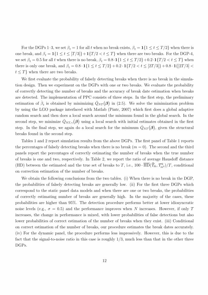
For the DGPs 1–3, we set βt = 1 for all t when no break exists, βt = 11 ≤ t ≤ T/2 when there is

one break, and βt = 11 ≤ t ≤ [T/3]+1T/2 < t ≤ T when there are two breaks. For the DGP-4,

we set βt = 0.5 for all t when there is no break, βt = 0.8 ·11 ≤ t ≤ T/2+0.2 ·1T/2 < t ≤ T when

there is only one break, and βt = 0.8 · 11 ≤ t ≤ T/2+ 0.2 · 1T/2 < t ≤ [2T/3]+ 0.8 · 1[2T/3] <

t ≤ T when there are two breaks.

We first evaluate the probability of falsely detecting breaks when there is no break in the simula-

tion design. Then we experiment on the DGPs with one or two breaks. We evaluate the probability

of correctly detecting the number of breaks and the accuracy of break date estimation when breaks

are detected. The implementation of PPC consists of three steps. In the first step, the preliminary

estimation of βt is obtained by minimizing QNT

(β)

in (2.5). We solve the minimization problem

by using the LGO package interfaced with Matlab (Pintr, 2007) which first does a global adaptive

random search and then does a local search around the minimum found in the global search. In the

second step, we minimize QNT,γ

(β)

using a local search with initial estimates obtained in the first

step. In the final step, we again do a local search for the minimum QNT

(β), given the structural

breaks found in the second step.

Tables 1 and 2 report simulation results from the above DGPs. The first panel of Table 1 reports

the percentages of falsely detecting breaks when there is no break (m = 0). The second and the third

panels report the percentages of correctly estimating the number of breaks when the true number

of breaks is one and two, respectively. In Table 2, we report the ratio of average Hausdoff distance

(HD) between the estimated and the true set of breaks to T , i.e., 100 · HD(Tm, T 0m0)/T , conditional

on correction estimation of the number of breaks.

We obtain the following conclusions from the two tables. (i) When there is no break in the DGP,

the probabilities of falsely detecting breaks are generally low. (ii) For the first three DGPs which

correspond to the static panel data models and when there are one or two breaks, the probabilities

of correctly estimating number of breaks are generally high. In the majority of the cases, these

probabilities are higher than 95%. The detection procedure performs better at lower idiosyncratic

noise levels (e.g., σ = 0.5) and the performance improves when N increases. However, if only T

increases, the change in performance is mixed, with lower probabilities of false detections but also

lower probabilities of correct estimation of the number of breaks when they exist. (iii) Conditional

on correct estimation of the number of breaks, our procedure estimates the break dates accurately.

(iv) For the dynamic panel, the procedure performs less impressively. However, this is due to the

fact that the signal-to-noise ratio in this case is roughly 1/3, much less than that in the other three

DGPs.

12

Table 1: The probabilities for falsely detecting breaks when there are none and of correctly detecting

the breaks when there are breaks

DGP σ N=T=40 N=T=80 N=80,T=40 N=40,T=80

m = 0, % of falsely detecting breaks when there are none.

0.5 0.8 0.4 0 01

1 0.8 0.4 0.4 0.8

0.5 0.8 0.8 0 0.42

1 2.8 0.8 0 1.6

0.5 1.2 0 0 1.23

1 1.2 0.4 0.4 3.2

0.5 0.4 0.4 0 0.44

1 2.4 0.8 0.8 0.4

m = 1, % of correctly detecting one break

0.5 99.6 94.8 99.6 96.81

1 96.8 91.6 99.6 79.2

0.5 94.8 98.4 100 92.82

1 94.4 90.8 100 81.2

0.5 98.8 98 99.2 95.63

1 96.4 96.4 98.8 89.6

0.5 74.4 82.4 90 61.24

1 72.8 88.4 90.8 70.8

m = 2, % of correctly detecting two breaks

0.5 99.6 98 100 94.81

1 94.8 93.2 99.2 87.2

0.5 96.8 98 100 962

1 90.8 93.2 98.4 82.8

0.5 99.6 97.2 100 96.83

1 96.8 93.6 98.4 92.4

0.5 64.8 82.8 81.6 50.84

1 62.8 84.4 86.4 61.2

13

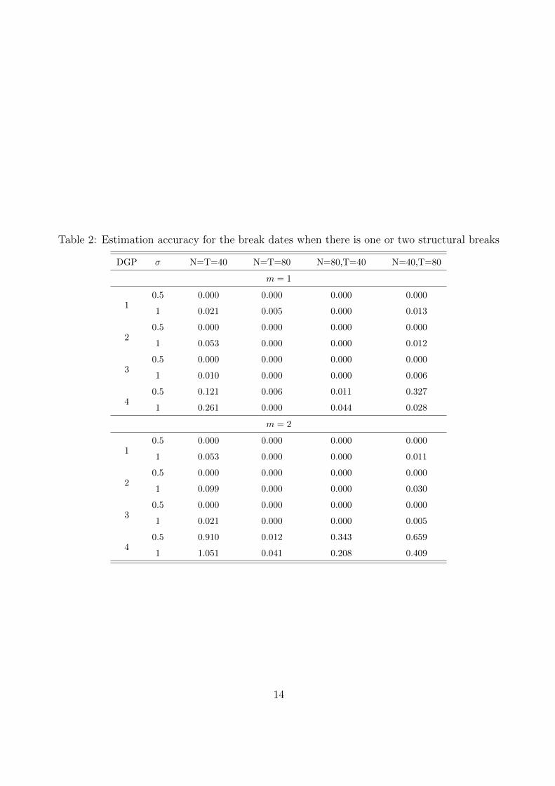
Table 2: Estimation accuracy for the break dates when there is one or two structural breaks

DGP σ N=T=40 N=T=80 N=80,T=40 N=40,T=80

m = 1

0.5 0.000 0.000 0.000 0.0001

1 0.021 0.005 0.000 0.013

0.5 0.000 0.000 0.000 0.0002

1 0.053 0.000 0.000 0.012

0.5 0.000 0.000 0.000 0.0003

1 0.010 0.000 0.000 0.006

0.5 0.121 0.006 0.011 0.3274

1 0.261 0.000 0.044 0.028

m = 2

0.5 0.000 0.000 0.000 0.0001

1 0.053 0.000 0.000 0.011

0.5 0.000 0.000 0.000 0.0002

1 0.099 0.000 0.000 0.030

0.5 0.000 0.000 0.000 0.0003

1 0.021 0.000 0.000 0.005

0.5 0.910 0.012 0.343 0.6594

1 1.051 0.041 0.208 0.409

14

5 Conclusions

In this paper, we study the estimation of the panel data models with interactive fixed effects and

multiple structural breaks, which substantially generalizes the existing work which either considers

the panel models with interactive fixed effects but no structural break (c.f., Bai, 2009), or the panel

models with multiple structural breaks but under cross-sectional independence (c.f., Qian and Su,

2014). We develop a novel PPC estimation procedure with the AGF LASSO penalty function to

consistently estimate both the regression coefficients and the factor loadings. Under some regularity

conditions, we show that both the unknown number of structural breaks and the unobservable break

dates can be consistently estimated. To further improve the convergence rates, we also estimate the

regression coefficients (in different regimes) through the post-LASSO method and then establish the

asymptotic distribution theory of the resulting estimators. In particular, the developed shrinkage

estimation methodology and the asymptotic theory are also applicable to the case of dynamic panel

data. We introduce a data-driven method to determine the tuning parameter involved in the PPC

estimation procedure. The simulation studies show that the proposed PPC method has an high

probability of correctly estimating the number of breaks when the structural breaks exist in the

simulation design, and a low probability of false detection when there is no structural break.

Appendix

We first give in Appendix A some regularity conditions that are used to derive the asymptotic

results, and then provide the proofs of the theoretical results in Section 3 as well as some tech-

nical lemmas in Appendix B. The proofs of the technical lemmas are given in Appendix C of the

supplemental document.

A Assumptions

We next list some mild assumptions which are sufficient to prove the asymptotic results stated in

Section 3, although some of them may not be the weakest possible.

Assumption 1 (i) There exist two positive definite matrices ΣF and ΣΛ such that 1TF 0′F 0 P→

ΣF and 1N

Λ0′Λ0 P→ ΣΛ. Furthermore, both the common factors f 0t and the factor loadings λ0

i have

finite 8-th moment.

15

(ii) Let the regressor Xt satisfy max1≤t≤T ‖Xt‖ = OP (N1/2) and

cx ≤ infΛ

min1≤t≤T

µmin

(N−1X ′tMΛXt

)≤ sup

Λmax

1≤t≤Tµmax

(N−1X ′tMΛXt

)≤ c∗x,

where 0 < cx < c∗x <∞, and supΛ and infΛ are taken with respect to Λ such that 1N

Λ′Λ = IR0 .

(iii) The idiosyncratic error term εit satisfies E[εit] = 0 and E[|εit|8] < C for each i and t, where C is

a bounded positive constant. Furthermore,

max1≤s,t≤T

E[‖X ′tεs‖2

]= O(N), max

1≤t≤TE[‖Λ0′εt‖2

]= O(N),

E[‖Λ0′εF 0‖2

]= O(NT ), max

1≤i,j≤NE[∥∥ T∑

t=1

T∑s=1

εitεjsγtγ′s

∥∥2]

= O(T 2), and

max1≤i,j≤N

E[∥∥ T∑

t=1

T∑s=1

εitεjsε′tεs∥∥2]

= O(N2T 2),

where γt can be either 1 or f 0t .

(iv) Letting ξij =∑T

t=1 εitεjt, there exists σij > 0 such that∣∣E[ξij]

∣∣ ≤ σijT , Var(ξij) = O(T )

and∑N

i=1

∑Nj=1 σ

2ij = O(N). Letting ηts =

∑Ni=1 εitεis, we have max1≤t≤T E

[∑Ts=1 η

2ts

]= O(N2 +

NT ) and E[∥∥∑T

t=1

∑Ts=1 f

0′t ηtsf

0s

∥∥2]= O(N2T 2).

Assumption 2 (i) The tuning parameter γ satisfies γ = o (1) and γ∆−κNT δNT = O(1), where δNT =

min(√T ,√N) and ∆NT = min1≤j≤m0

∥∥α0j+1 − α0

j

∥∥. Furthermore, ∆∗NT ≡ max1≤j≤m0

∥∥α0j+1 − α0

j

∥∥ =

O(1).

(ii) Let γδκ+1NT →∞ as (N, T )→∞.

(iii) Let δNT∆NT →∞ as (N, T )→∞.

Assumption 3 (i) For j, k = 1, · · · ,m0 + 1, there exist p × p positive definite matrices Φj and Φ∗jksuch that

1

NT

T 0j −1∑

t=T 0j−1

X ′tMΛ0XtP→ Φj and

1

NT 2

T 0j −1∑

t=T 0j−1

T 0k−1∑

s=T 0k−1

χstX′tMΛ0Xs

P→ Φ∗jk,

where χst = f 0′s

(1TF 0′F 0

)+f 0t . Furthermore, Ω0 ≡ Φ−Φ∗ is assumed to be positive definite, where

Φ = diag(Φ1, · · · ,Φm0+1) and

Φ∗ =

Φ11 Φ12 · · · Φ1,m0+1

Φ21 Φ22 · · · Φ2,m0+1

......

......

Φm0+1,1 Φm0+1,2 · · · Φm0+1,m0+1

.

16

(ii) There exist 0 < τ j < 1, j = 1, · · · ,m0 + 1, such that

1

T(T 0

j − T 0j−1)→ τ j,

m0+1∑j=1

τ j = 1.

(iii) Let

max1≤t≤T

E(A2t ) = O(N2(N + T )), δ3

NT/√NT →∞

as (N, T )→∞, where At =∑T

s=1 Λ0′εsε′sεt.

(iv) LettingWj,NT = 1NT

∑T 0j −1

t=T 0j−1

X ′tMΛ0(εt−ε∗t ) for j = 1, · · · ,m0+1 andWNT = (W ′1,NT , · · · ,W ′

m0+1,NT )′,

there exist BNT (3) and Ω1 such that

√NT [WNT −BNT (3)]

D−→ N(0,Ω1

).

Remark A.1. Assumption 1 imposes some standard moment conditions on Xit, f0t , λ0

i and εit, which

are analogous to those in the existing literature such as Bai and Ng (2002), Bai (2009), Lu and Su

(2013) and Bai and Li (2014). Assumptions 1 (iii) and (iv) allow weak form of cross-sectional depen-

dence and serial dependence among Xit, f0t , λ0

i and εit. In particular, unlike Pesaran (2006) and Bai

(2009), we do not assume independence between εit and (Xjs, f0s , λ

0j) for all i, j, t, s, and our theories

are thus applicable to the dynamic autoregressive panel data models with interactive fixed effects.

Assumption 2 imposes some mild restrictions on the tuning parameter γ and the jump sizes of the

regression coefficients, which can be easily justified. For example, assuming that the jump sizes are

bounded away from zero and infinity, we may show that Assumption 2 is satisfied if γδNT = O(1)

and γδκ+1NT →∞. Assumption 3 imposes some additional conditions for the proof of the asymptotic

distribution theory of the post-LASSO estimation, which can be verified under some primitive con-

ditions. For example, if we assume that εit, λ0i are independent across i and for each i, εit is a

martingale difference sequence with respect to the σ-field generated by (εi,t−1, . . . , εi1, f0t−1, . . . , f

01 , λ

0i )

and εit, Xit satisfy some strongly mixing conditions, then the moment condition in Assumption

3(iii) holds.

B Proof of the results in Section 3

In this appendix, we give the detailed proofs of the asymptotic results in Section 3. We start with

a lemma on the convergence rates of the preliminary estimators βt, t = 1, 2, · · · , T , whose proof is

provided in Appendix C of the supplemental document.

17

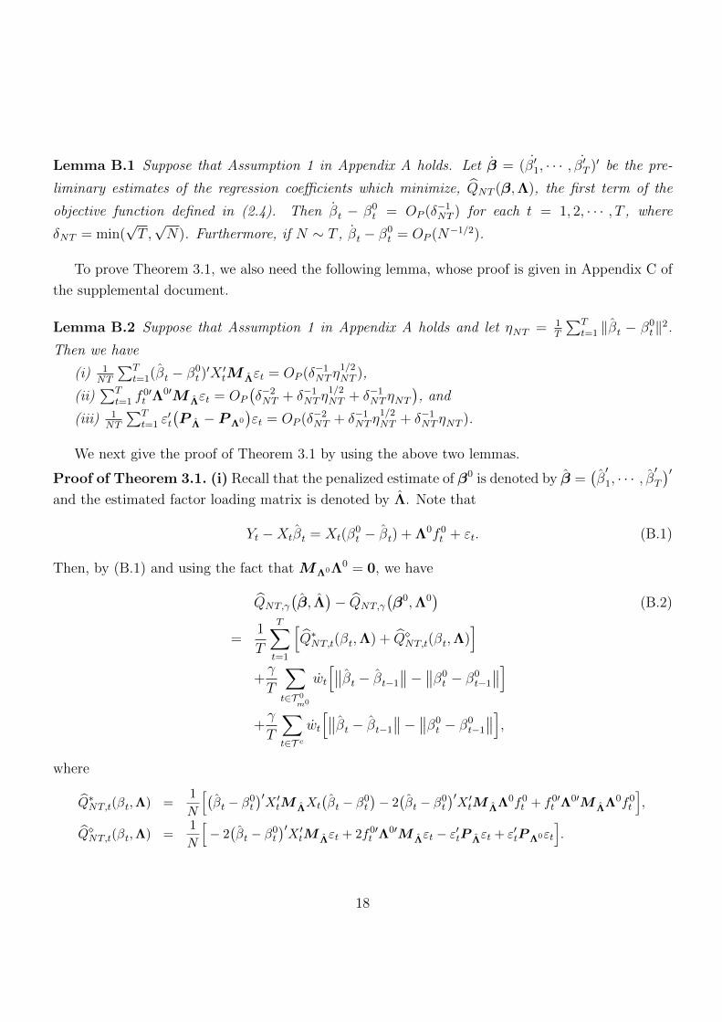
Lemma B.1 Suppose that Assumption 1 in Appendix A holds. Let β = (β′1, · · · , β′T )′ be the pre-

liminary estimates of the regression coefficients which minimize, QNT (β,Λ), the first term of the

objective function defined in (2.4). Then βt − β0t = OP (δ−1

NT ) for each t = 1, 2, · · · , T , where

δNT = min(√T ,√N). Furthermore, if N ∼ T , βt − β0

t = OP (N−1/2).

To prove Theorem 3.1, we also need the following lemma, whose proof is given in Appendix C of

the supplemental document.

Lemma B.2 Suppose that Assumption 1 in Appendix A holds and let ηNT = 1T

∑Tt=1 ‖βt − β0

t‖2.

Then we have

(i) 1NT

∑Tt=1(βt − β0

t )′X ′tM Λεt = OP (δ−1

NTη1/2NT ),

(ii)∑T

t=1 f0′t Λ0′M Λεt = OP

(δ−2NT + δ−1

NTη1/2NT + δ−1

NTηNT), and

(iii) 1NT

∑Tt=1 ε

′t

(P Λ − PΛ0

)εt = OP (δ−2

NT + δ−1NTη

1/2NT + δ−1

NTηNT ).

We next give the proof of Theorem 3.1 by using the above two lemmas.

Proof of Theorem 3.1. (i) Recall that the penalized estimate of β0 is denoted by β =(β′1, · · · , β

′T

)′and the estimated factor loading matrix is denoted by Λ. Note that

Yt −Xtβt = Xt(β0t − βt) + Λ0f 0

t + εt. (B.1)

Then, by (B.1) and using the fact that MΛ0Λ0 = 0, we have

QNT,γ

(β, Λ

)− QNT,γ

(β0,Λ0

)(B.2)

=1

T

T∑t=1

[Q∗NT,t(βt,Λ) + QNT,t(βt,Λ)

]+γ

T

∑t∈T 0

m0

wt

[∥∥βt − βt−1

∥∥− ∥∥β0t − β0

t−1

∥∥]+γ

T

∑t∈T c

wt

[∥∥βt − βt−1

∥∥− ∥∥β0t − β0

t−1

∥∥],where

Q∗NT,t(βt,Λ) =1

N

[(βt − β0

t

)′X ′tM ΛXt

(βt − β0

t

)− 2(βt − β0

t

)′X ′tM ΛΛ0f0

t + f0′t Λ0′M ΛΛ0f0

t

],

QNT,t(βt,Λ) =1

N

[− 2(βt − β0

t

)′X ′tM Λεt + 2f0′

t Λ0′M Λεt − ε′tP Λεt + ε′tPΛ0εt

].

18

As β0t − β0

t−1 = 0 for t ∈ T c, the last term on the right hand side of (B.2) satisfies that

γ

T

∑t∈T c

wt

[∥∥βt − βt−1

∥∥− ∥∥β0t − β0

t−1

∥∥] =γ

T

∑t∈T c

wt∥∥βt − βt−1

∥∥ ≥ 0. (B.3)

By the triangle inequality and Lemma B.1, we can prove that

∑t∈T 0

m0

wt

[∥∥βt − βt−1

∥∥− ∥∥β0t − β0

t−1

∥∥] ≤ OP (∆−κNT )T∑t=1

∥∥βt − β0t

∥∥≤ OP (∆−κNT )T 1/2

( T∑t=1

∥∥βt − β0t

∥∥2)1/2,

which, in conjunction with Assumption 2 (i) in Appendix A, indicates that

γ

T

∑t∈T 0

m0

wt

[∥∥βt − βt−1

∥∥− ∥∥β0t − β0

t−1

∥∥] = OP (δ−1NT )

( 1

T

T∑t=1

∥∥βt − β0t

∥∥2)1/2= OP (δ−1

NT η1/2NT ). (B.4)

By Lemma B.2, we can readily show that

1

N

T∑t=1

QNT,t(βt,Λ) = OP (δ−2NT + δ−1

NTη1/2NT + δ−1

NTηNT ). (B.5)

Combining (B.4) and (B.5), we have

QNT,γ

(β, Λ

)− QNT,γ

(β0,Λ0

)≥ 1

T

T∑t=1

Q∗NT,t(βt,Λ) +OP (δ−2NT + δ−1

NTη1/2NT + δ−1

NTηNT ). (B.6)

Define the vectors:

dβ = β − β0 and dΛ =1

N1/2vec(M ΛΛ0),

where vec(·) denotes the vectorization of a matrix; and define the matrices:

A =1

Ndiag

(X ′1M ΛX1, · · · , X ′TM ΛXT

), B = (F 0′F 0)⊗ IN , and

C =1

N1/2

[f 0

1 ⊗M ΛX1, · · · , f 0T ⊗M ΛXT

],

19

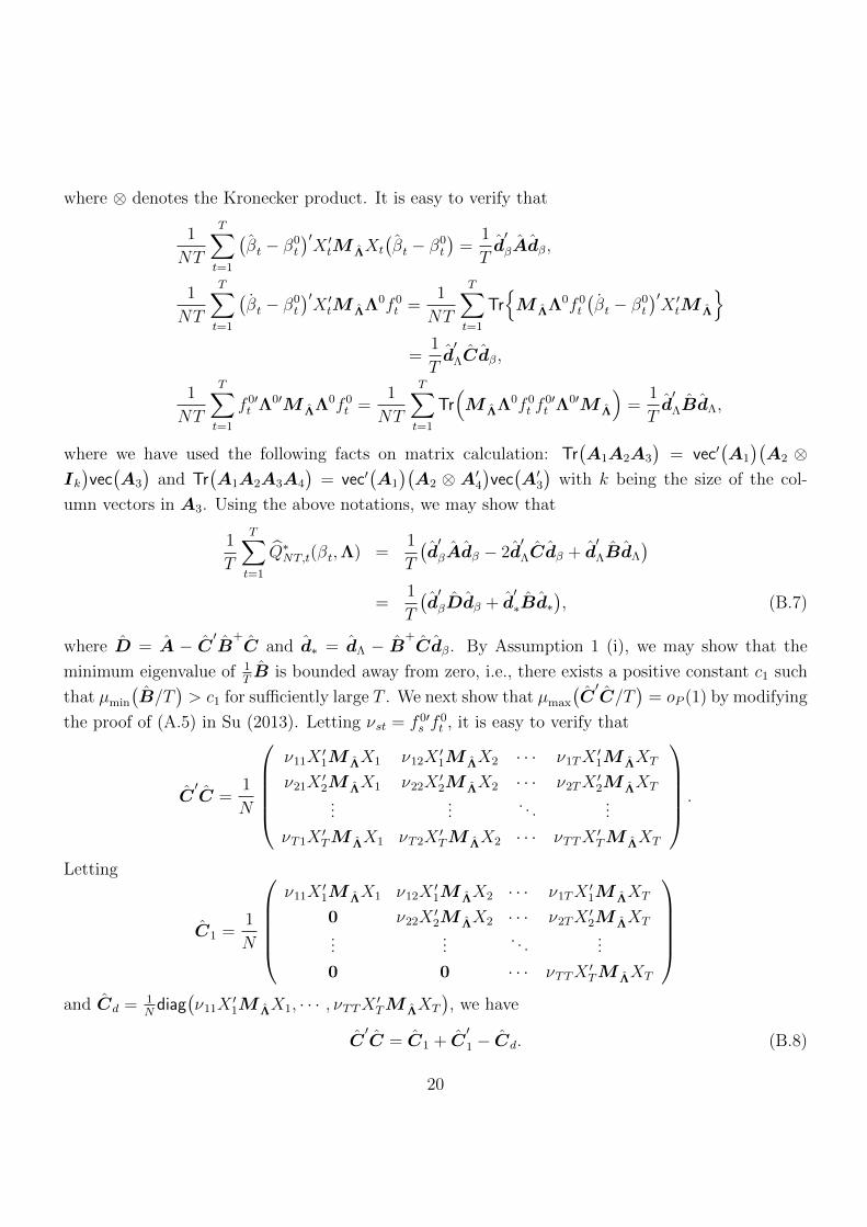
where ⊗ denotes the Kronecker product. It is easy to verify that

1

NT

T∑t=1

(βt − β0

t

)′X ′tM ΛXt

(βt − β0

t

)=

1

Td′βAdβ,

1

NT

T∑t=1

(βt − β0

t

)′X ′tM ΛΛ0f 0

t =1

NT

T∑t=1

TrM ΛΛ0f 0

t

(βt − β0

t

)′X ′tM Λ

=

1

Td′ΛCdβ,

1

NT

T∑t=1

f 0′t Λ0′M ΛΛ0f 0

t =1

NT

T∑t=1

Tr(M ΛΛ0f 0

t f0′t Λ0′M Λ

)=

1

Td′ΛBdΛ,

where we have used the following facts on matrix calculation: Tr(A1A2A3

)= vec′

(A1

)(A2 ⊗

Ik)vec(A3

)and Tr

(A1A2A3A4

)= vec′

(A1

)(A2 ⊗ A′4

)vec(A′3)

with k being the size of the col-

umn vectors in A3. Using the above notations, we may show that

1

T

T∑t=1

Q∗NT,t(βt,Λ) =1

T

(d′βAdβ − 2d

′ΛCdβ + d

′ΛBdΛ

)=

1

T

(d′βDdβ + d

′∗Bd∗

), (B.7)

where D = A − C′B

+C and d∗ = dΛ − B

+Cdβ. By Assumption 1 (i), we may show that the

minimum eigenvalue of 1TB is bounded away from zero, i.e., there exists a positive constant c1 such

that µmin

(B/T

)> c1 for sufficiently large T . We next show that µmax

(C′C/T

)= oP (1) by modifying

the proof of (A.5) in Su (2013). Letting νst = f 0′s f

0t , it is easy to verify that

C′C =

1

N

ν11X

′1M ΛX1 ν12X

′1M ΛX2 · · · ν1TX

′1M ΛXT

ν21X′2M ΛX1 ν22X

′2M ΛX2 · · · ν2TX

′2M ΛXT

......

. . ....

νT1X′TM ΛX1 νT2X

′TM ΛX2 · · · νTTX

′TM ΛXT

.

Letting

C1 =1

N

ν11X

′1M ΛX1 ν12X

′1M ΛX2 · · · ν1TX

′1M ΛXT

0 ν22X′2M ΛX2 · · · ν2TX

′2M ΛXT

......

. . ....

0 0 · · · νTTX′TM ΛXT

and Cd = 1

Ndiag

(ν11X

′1M ΛX1, · · · , νTTX ′TM ΛXT

), we have

C′C = C1 + C

′1 − Cd. (B.8)

20

By the fact that the eigenvalues of a block upper/lower triangular matrix are the combined eigenvalues

of its diagonal block matrices, Weyl’s inequality, and Assumptions 1 (i)-(ii), we have

T−1µmax(C′C) ≤ T−12µmax(C1)− µmin(Cd)

≤ 2T−1 max1≤t≤T

∥∥f 0t

∥∥2µmax

(N−1X ′tM ΛXt

)= OP (T−1)oP (T 1/4)OP (1) = oP (T−3/4),

where we use the fact that max1≤t≤T ‖f 0t ‖2 = OP

(T 1/4

)under Assumption 1 (i) by the Markov

inequality. On the other hand, we note that the minimum eigenvalue of A is positive and bounded

away from zero. Hence, the matrix D is asymptotically positive definite as its minimum eigenvalue

is positive and bounded away from zero by using the above facts. Then, by (B.7) and (B.8), we can

readily show that there exist two positive constants c2 and c3 such that

c2

T‖dβ‖2 + c3‖d∗‖2 ≤ 1

T

T∑t=1

Q∗NT,t(βt,Λ), (B.9)

which indicates that

c2

T‖dβ‖2 + c3‖d∗‖2 +OP (δ−2

NT + δ−1NTη

1/2NT + δ−1

NTηNT ) ≤ QNT

(β, Λ

)− QNT

(β0,Λ0

). (B.10)

Letting both sides in (B.10) multiply δ2NT and noting that ‖dβ‖2 = TηNT and QNT

(β, Λ

)−

QNT

(β0,Λ0

)≤ 0, we readily show that

c2 + oP (1)

T‖δNT dβ‖2 +OP (1) ·

( 1

T‖δNT dβ‖2

)1/2+OP (1) ≤ 0. (B.11)

When 1T‖δNT dβ‖2 is sufficiently large, the first term on the right hand side of (B.11) would dominate

the other two terms, which would lead to a contradiction. Hence, we must have 1T‖δNT dβ‖2 is

stochastically bounded, which completes the proof of Theorem 3.1 (i).

(ii) The proof for the point-wise convergence result is analogous, and details are omitted here.

We have thus completed the proof of Theorem 3.1.

Proof of Theorem 3.2. To prove the sparsity, it is equivalent to show

P(∥∥θt∥∥ 6= 0 for some t ∈ T c

)→ 0 (B.12)

as (N, T )→∞. We consider two cases: (i) 2 ≤ t ≤ T − 1 and t ∈ T c; and (ii) t = T and t ∈ T c.

21

For case (i), there would be two possible circumstances: (i.1) t + 1 = T 0j ∈ T 0

m0 for some

j = 1, · · · ,m0; and (i.2) t + 1 ∈ T c. We invoke subdifferential calculus (e.g., Bersekas, 1995,

Appendix B.5) to obtain the following Karush-Kuhn-Tucker condition with respect to βt to the

objective function in (2.4):

δNT

[−2

NX ′tM Λ

(Yt −Xtβt

)+ γwt

βt − βt−1∥∥βt − βt−1

∥∥ − γwt+1

βt+1 − βt∥∥βt+1 − βt∥∥] = 0, (B.13)

where for any p × 1 vector a, a/‖a‖ is defined as an arbitrary p × 1 vector with Frobenius norm

smaller than or equal to 1 in case ‖a‖ = 0. Let UNT,1 = 1NX ′tM Λ

(Yt −Xtβt

), UNT,2 = γwt

βt−βt−1∥∥βt−βt−1

∥∥and UNT,3 = γwt+1

βt+1−βt∥∥βt+1−βt∥∥ . Following the proof of Theorem 3.1, we may show that

δNT‖UNT,1‖ = OP (1). (B.14)

If circumstance (i.1) holds, by Lemma B.1 and Assumption 2 (iii), we have

wt+1 = ‖βt+1 − βt‖−κ ≤[

min1≤j≤m0

∥∥α0j+1 − α0

j

∥∥+OP (δ−1NT )]−κ

= OP (∆−κNT ), (B.15)

which together with Assumption 2 (i), indicates that

δNT‖UNT,3‖ = OP (γδNT∆−κNT ) = OP (1). (B.16)

However, for case (i) with 2 ≤ t ≤ T − 1 and t ∈ T c, by Lemma B.1, we may show that w.p.a.1

wt = ‖βt − βt−1‖−κ ≥ CδκNT , (B.17)

for some positive constant C. Hence, it is not difficult to see that when θt 6= 0,

δNT‖UNT,2‖ ≥ Cγδκ+1NT →∞ (B.18)

by using Assumption 2 (ii). By (B.14), (B.16) and (B.18), the equation (B.13) cannot hold as

(N, T )→∞. Hence, θt can only take the value of 0 at which ||θt|| is not differentiable. Furthermore,

as an implication of the above result, if t = T 0j − 1 ∈ T c for some j = 1, · · · ,m0, then we have

δNTγwtβt − βt−1∥∥βt − βt−1

∥∥ = δNTγwT 0j −1

βT 0j −1 − βT 0

j −2∥∥βT 0j −1 − βT 0

j −2

∥∥ = OP (1). (B.19)

22

We next prove (B.12) for circumstance (i.2). Following the above argument, we can show that

when t = T 0j − 2 and θT 0

j −2 6= 0,

δNTN

X ′tM Λ

(Yt −Xtβt

)= OP (1), δNTγwt

βt − βt−1∥∥βt − βt−1

∥∥ →∞, (B.20)

which, together with (B.19), implies that (B.13) cannot hold as (N, T )→∞. Hence, θT 0j −2 can only

be 0. Deducting in this way until we reach t = T 0j−1 + 1 ∈ T c, we can complete the proof of sparsity

for case (i).

For case (ii), note that the consequence of the Karush-Kuhn-Tucker condition with respect to βTleads to

δNT

[ 1

NX ′TM Λ

(YT −XT βT

)+ γwT

βT − βT−1∥∥βT − βT−1

∥∥] = 0. (B.21)

As there is only one penalty term in (B.21), the proof is much simpler than that for case (i). Hence,

we omit the details here.

We have completed the proof of Theorem 3.2.

Proof of Corollary 3.3. By Theorem 3.2, as (N, T ) → ∞, no time point in T c can be identified

as the break time, which implies that m ≤ m0. On the other hand, by Theorem 3.1, for any t ∈ T 0m0 ,

θt = βt − βt−1 = β0t − β0

t−1 +OP (δ−1NT ) = θ0

t +OP (δ−1NT ),

which indicates that ‖θ0t‖ = OP (δ−1

NT ) if θt = 0 (i.e., t ∈ T 0m0 is not identified as a break time).

However, the conclusion ‖θ0t‖ = OP (δ−1

NT ) would violate the condition δNT∆NT → ∞. Hence, each

time point in T 0m0 must be identified as the break time, which implies that m = m0 w.p.a.1 and thus

both the results (i) and (ii) are proved.

Before proving the asymptotic distribution theory for the post-LASSO estimator in Theorem 3.4,

we first give the following lemma which will be used in the proof. The proof of this lemma is given

in Appendix C of the supplemental document.

Lemma B.3 Suppose that the conditions in Theorem 3.4 holds. Let Λm0 ≡ Λ(T 0m0) be the infeasible

estimate of the factor loadings in the post-LASSO estimation procedure, H =(

1TF 0′F 0

)(1N

Λ0′Λm0

)V

+

NT ,

and αm0 ≡ αm0(T 0m0), where V NT will be defined later in (B.25). Then, for j = 1, · · · ,m0, we have

(i)

1

NT

T 0j −1∑

t=T 0j−1

X ′t(M Λm0

−MΛ0

)εt = −BNT,j(2, 1) +OP

(δ−1NT (αm0 −α0)

)+OP

(δ−3NT

)

23

and (ii)

1

NT

T 0j −1∑

t=T 0j−1

X ′tM Λm0

(Λ0 − Λm0H

+)f0t

= − 1

NT

T 0j −1∑

t=T 0j−1

X ′tMΛ0ε∗t +[Φ∗j1, · · · ,Φ∗j,m0+1

](αm0 −α0)−

BNT,j(1) +BNT,j(2, 2) +OP (δ−1NT (αm0 −α0)) +OP

(δ−3NT

),

where Φ∗jk, 1 ≤ j, k ≤ m0 + 1, are defined in Assumption 3 (i), and BNT,j(1), BNT,j(2, 1), and

BNT,j(2, 2), j = 1, · · · ,m0 + 2, are defined as in Theorem 3.4.

We are now ready to prove Theorem 3.4.

Proof of Theorem 3.4. Let GT =Tj = T 0

j for j = 1, ...,m0

. By Corollary 3.3, we readily have

P√

NT(αm −α0) ∈ C

∣∣m = m0

= P√

NT(αm −α0) ∈ C,GT

∣∣m = m0

+P√

NT(αm −α0) ∈ C,GcT

∣∣m = m0

= P√

NT(αm0 −α0) ∈ C

+ o(1), (B.22)

where C ⊂ Rp(m0+1), GcT is the complement of GT and αm0 ≡ αm0(Tm0) is the infeasible estimate of

α0. Hence, throughout the proof, we can replace m and Tj (j = 1, · · · , m) by m0 and T 0j , respectively,

which would not affect the asymptotic distribution of the post-LASSO estimator.

Letting m = m0 and Tj = T 0j in the objective function (3.1), we have

QNT(αm0 ,Λ,F ; T 0

m0

)=

m0+1∑j=1

1

NT

T 0j −1∑

t=T 0j−1

(Yt −Xtαj −Λft

)′(Yt −Xtαj −Λft

),

and

minF

QNT(αm0 ,Λ,F ; T 0

m0

)=

m0+1∑j=1

1

NT

T 0j −1∑

t=T 0j−1

(Yt −Xtαj

)′MΛ

(Yt −Xtαj

). (B.23)

Recall that Λm0 ≡ Λ(T 0m0) is defined in Lemma B.3. Let

ΦNT (Λm0) = diag

Φ1(Λm0), · · · , Φm0+1(Λm0)

and

ΞNT (Λm0) =[Ξ1(Λm0)′, · · · , Ξm0+1(Λm0)′

]′,

24

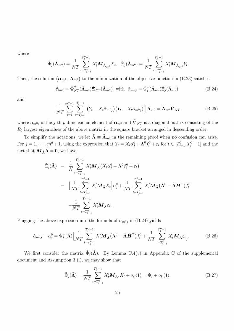
where

Φj(Λm0) =1

NT

T 0j −1∑

t=T 0j−1

X ′tM Λm0Xt, Ξj(Λm0) =

1

NT

T 0j −1∑

t=T 0j−1

X ′tM Λm0Yt.

Then, the solution(αm0 , Λm0

)to the minimization of the objective function in (B.23) satisfies

αm0 = Φ+

NT (Λm0)ΞNT (Λm0) with αm0j = Φ+j (Λm0)Ξj(Λm0), (B.24)

and [ 1

NT

m0+1∑j=1

Tj−1∑t=Tj−1

(Yt −Xtαm0j

)(Yt −Xtαm0j

)′]Λm0 = Λm0V NT , (B.25)

where αm0j is the j-th p-dimensional element of αm0 and V NT is a diagonal matrix consisting of the

R0 largest eigenvalues of the above matrix in the square bracket arranged in descending order.

To simplify the notations, we let Λ ≡ Λm0 in the remaining proof when no confusion can arise.

For j = 1, · · · ,m0 + 1, using the expression that Yt = Xtα0j + Λ0f 0

t + εt for t ∈ [T 0j−1, T

0j − 1] and the

fact that M ΛΛ = 0, we have

Ξj(Λ) =1

N

T 0j −1∑

t=T 0j−1

X ′tM Λ

(Xtα

0j + Λ0f 0

t + εt)

=[ 1

NT

T 0j −1∑

t=T 0j−1

X ′tM ΛXt

]α0j +

1

NT

T 0j −1∑

t=T 0j−1

X ′tM Λ

(Λ0 − ΛH

+)f 0t

+1

NT

T 0j −1∑

t=T 0j−1

X ′tM Λεt.

Plugging the above expression into the formula of αm0j in (B.24) yields

αm0j − α0j = Φ+

j (Λ)[ 1

NT

T 0j −1∑

t=T 0j−1

X ′tM Λ

(Λ0 − ΛH

+)f 0t +

1

NT

T 0j −1∑

t=T 0j−1

X ′tM Λεt

]. (B.26)

We first consider the matrix Φj(Λ). By Lemma C.4(v) in Appendix C of the supplemental

document and Assumption 3 (i), we may show that

Φj(Λ) =1

NT

T 0j −1∑

t=T 0j−1

X ′tMΛ0Xt + oP (1) = Φj + oP (1), (B.27)

25

with Φj defined in Assumption 3 (i) in Appendix A. Hence, we have as (N, T )→∞,

ΦNT (Λm0) = ΦNT (Λ)P→ Φ (B.28)

with Φ = diag

Φ1, · · · ,Φm0+1

.

We next consider the term 1NT

∑T 0j −1

t=T 0j−1

X ′tM Λεt. By Lemma B.3 (i),

1

NT

T 0j −1∑

t=T 0j−1

X ′tM Λεt =1

NT

T 0j −1∑

t=T 0j−1

X ′tMΛ0εt −BNT,j(2, 1) +

OP

(δ−1NT (αm0 −α0)

)+OP

(δ−3NT

). (B.29)

On the other hand, by Lemma B.3 (ii), we have

1

NT

T 0j −1∑

t=T 0j−1

X ′tM Λm0

(Λ0 − Λm0H

+)f 0t

= − 1

NT

T 0j −1∑

t=T 0j−1

X ′tMΛ0ε∗t +[Φ∗j1, · · · ,Φ∗j,m0+1

](αm0 −α0)−

BNT,j(1) +BNT,j(2, 2) +OP

(δ−1NT (αm0 −α0)

)+OP

(δ−3NT

). (B.30)

Recall thatBNT (1) =[BNT,1(1)′, · · · , BNT,m0+1(1)′

]′,BNT (2) = [BNT,1(2, 1)′−BNT,1(2, 2)′, · · · , BNT,m0+1(2, 1)′−

BNT,m0+1(2, 2)′]′, and Ω0 = Φ − Φ∗. By the definition of WNT in Assumption 3 (iv), (B.24), and

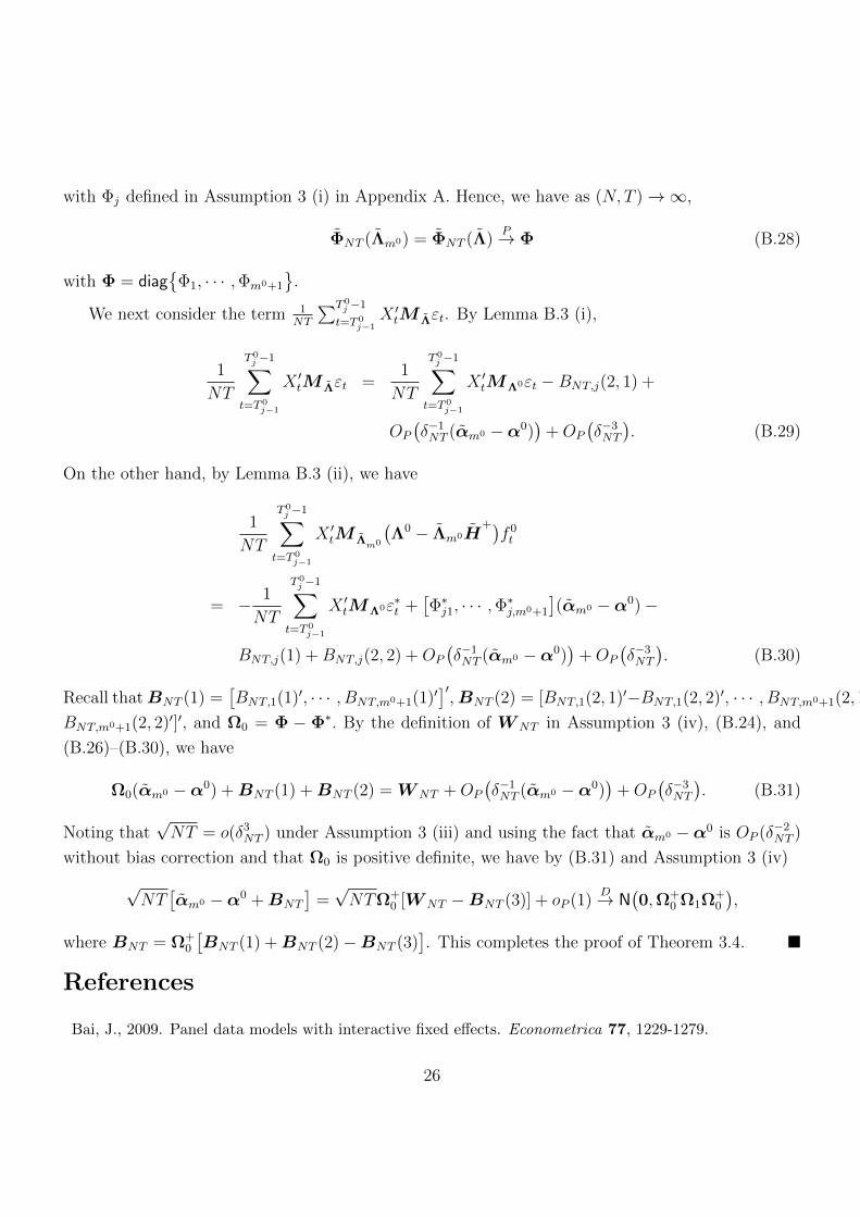
(B.26)–(B.30), we have

Ω0(αm0 −α0) +BNT (1) +BNT (2) = WNT +OP

(δ−1NT (αm0 −α0)

)+OP

(δ−3NT

). (B.31)

Noting that√NT = o(δ3

NT ) under Assumption 3 (iii) and using the fact that αm0 −α0 is OP (δ−2NT )

without bias correction and that Ω0 is positive definite, we have by (B.31) and Assumption 3 (iv)

√NT

[αm0 −α0 +BNT

]=√NTΩ+

0 [WNT −BNT (3)] + oP (1)D→ N

(0,Ω+

0 Ω1Ω+0

),

where BNT = Ω+0

[BNT (1) +BNT (2)−BNT (3)

]. This completes the proof of Theorem 3.4.

References

Bai, J., 2009. Panel data models with interactive fixed effects. Econometrica 77, 1229-1279.

26

Bai, J., 2010. Common breaks in means and variances for panel data. Journal of Econometrics 157, 78-92.

Bai, J., Li, K., 2014. Theory and methods of panel data models with interactive fixed effects. Annals of

Statistics 42, 142–170.

Bai, J., Ng, S., 2002. Determining the number of factors in approximate factor models. Econometrica 70,

191–221.

Bai, J., Perron, P., 1998. Estimating and testing liner models with multiple structural changes. Econo-

metrica 66, 47-78.

Baltagi, B. H., Feng, Q., Kao, C., 2013. Estimation of heterogeneous panels with structural breaks.

Working Paper, Syracuse University.

Bertsekas, D., 1995. Nonlinear Programming. Athena Scientific, Belmont, MA.

Csorgo, M., Horvath, L., 1997. Limit Theorems in Change-Point Analysis. Wiley Series in Probability

and Statistics.

De Watcher, S., Tzavalis, E., 2012. Detection of structural breaks in linear dynamic panel data models.

Computational Statistics and Data Analysis 56, 3020-3034.

Fan, J., Li, R., 2001. Variable selection via nonconcave penalized likelihood and it oracle properties.

Journal of American Statistical Association 96, 1348-1360.

Fan, J., Li, R., 2006. Statistical challenges with high dimensionality: feature selection in knowledge

discovery. Proceedings of the International Congress of Mathematicians (Sanz-Sole, M., Soria, J.,

Varona, J. L., Verdera, J., eds.) Vol. III, European Mathematical Society, Zurich, 595-622.

Harchaoui, Z., Levy-Leduc, C., 2010. Multiple change-point estimation with a total variation penalty.

Journal of the American Statistical Association 105, 1480-1493.

Kim, D., 2011. Estimating a common deterministic time trend break in large panels with cross sectional

dependence. Journal of Econometrics 164, 310-330.

Lu, X., Su, L., 2013. Shrinkage estimation of dynamic panel data models with interactive fixed effects.

Working paper, Singapore Management University.

Moon, H. R. Weidner, M., 2013. Dynamic linear panel data regression models with interactive fixed effects.

Working paper, University of Southern California.

27

Pesaran, M. H., 2006. Estimation and inference in large heterogeneous panels with a multifactor error

structure. Econometrica 74, 967-1012.

Qian, J., Su, L., 2013. Shrinkage estimation of regression models with multiple structural changes. Working

paper, Singapore Management University.

Qian, J., Su, L., 2014. Shrinkage estimation of common breaks in panel data models via adaptive group

fused Lasso. Working paper, Singapore Management University.

Qu, Z., Perron, P., 2007. Estimating and testing structural changes in multiple regressions. Econometrica

75, 459-502.

Su, L., 2013. Identifying latent grouped effects in panel data models with interactive fixed effects. Working

paper, Singapore Management University.

Tibshirani, R., Saunders, M., Rosset, S., Zhu, J., Knight, K., 2005. Sparsity and smoothness via the fused

Lasso. Journal of the Royal Statistical Society, Series B 67, 91-108.

Rinaldo, A., 2009. Properties and refinement of the fused Lasso. Annals of Statistics 37, 2922-2952.

Yuan, M., Lin, Y., 2006. Model selection and estimation in regression with grouped variables. Journal of

the Royal Statistical Society, Series B 68, 49-67.

Zou, H., 2006. The adaptive Lasso and its oracle properties. Journal of the American Statistical Association

101, 1418-1429.

28

Supplemental Document for

Panel Data Models with Interactive Fixed Effectsand Multiple Structural Breaks

By Degui Li, Junhui Qian, and Liangjun Su

University of York, Shanghai Jiao Tong University, and Singapore Management University

C Proofs of the technical lemmas

In this appendix we give detailed proofs of the technical lemmas used in Appendix B. Before proving

Lemma B.1 on the convergence rates of βt, we give some preliminary results. They are similar to the

corresponding results derived by Su (2013) by switching the role of F and Λ. Let b = (b′1, b′2, · · · , b′T )′

where bt is a p-dimensional column vector and let C be a positive constant whose value may change

from line to line.

Lemma C.1 Suppose that Assumption 1 in Appendix A holds. Then we have

(i) supb supΛ

∣∣∣ 1NT

∑Tt=1 b

′tX′tMΛεt

∣∣∣ = OP

(N−1/4 + T−1/4

),

(ii) supΛ

∣∣∣ 1NT

∑Tt=1 f

0′t Λ0′MΛεt

∣∣∣ = OP (N−1/4 + T−1/4),

(iii) supΛ

∣∣∣ 1NT

∑Tt=1 ε

′tPΛεt

∣∣∣ = OP (N−1/2 + T−1/2),

(iv) 1NT

∑Tt=1 ε

′tPΛ0εt = OP (N−1),

where supb is taken with respect to b such that ‖b‖ ≤ CT 1/2 and supΛ is taken with respect to Λ

such that 1N

Λ′Λ = IR0.

Proof of Lemma C.1. (i) Note that

1

NT

T∑t=1

b′tX′tMΛεt =

1

NT

T∑t=1

b′tX′tεt −

1

N2T

T∑t=1

b′tX′tΛΛ′εt

if 1N

Λ′Λ = IR0 . By Assumption 1 (iii) and the Cauchy-Schwarz inequality, we have

∣∣ T∑t=1

b′tX′tεt∣∣ =

( T∑t=1

‖bt‖2)1/2 ·

( T∑t=1

‖X ′tεt‖2)1/2

= OP (√NT ) (C.1)

29

for ‖b‖2 =∑T

t=1 ‖bt‖2 ≤ CT . On the other hand, by some elementary calculations, we have

∣∣ T∑t=1

b′tX′tΛΛ′εt

∣∣ ≤ T∑t=1

∣∣b′tX ′tΛΛ′εt∥∥ ≤ T∑

t=1

∥∥b′tX ′tΛ∥∥∥∥Λ′εt∥∥≤ max

1≤t≤T

∥∥X ′tΛ∥∥ T∑t=1

∥∥bt∥∥∥∥Λ′εt∥∥≤ max

1≤t≤T

∥∥X ′tΛ∥∥( T∑t=1

∥∥bt∥∥2)1/2( T∑

t=1

∥∥Λ′εt∥∥2)1/2

.

By the restriction on Λ and Assumption 1 (ii), we have

max1≤t≤T

∥∥X ′tΛ∥∥ = OP (N). (C.2)

On the other hand, similar to the proof of Lemma A.1 in Bai (2009), we have

T∑t=1

∥∥Λ′εt∥∥2=

T∑t=1

Tr(Λ′εtε

′tΛ)

=T∑t=1

N∑i1=1

N∑i2=1

Tr(λi1λ′i2

)εi1tεi2t

=N∑i1=1

N∑i2=1

Tr(λi1λ′i2

)T∑t=1

(εi1tεi2t − E[εi1tεi2t]

)+

N∑i1=1

N∑i2=1

Tr(λi1λ′i2

)T∑t=1

E[εi1tεi2t].

For the first term on the right hand side, it is easy to show that

∣∣∣ N∑i1=1

N∑i2=1

Tr(λi1λ′i2

)T∑t=1

(εi1tεi2t − E[εi1tεi2t]

)∣∣∣ ≤ ( N∑i1=1

λ2i1

N∑i2=1

λ2i2

)1/2

·( N∑i1=1

N∑i2=1

T∑t=1

[εi1tεi2t − E[εi1tεi2t]

]2)1/2

= OP (N) ·OP (NT 1/2) (C.3)

by the Cauchy-Schwarz inequality and Assumption 1 (iv) which indicates that

T∑t=1

εi1tεi2t − E[εi1tεi2t]

= ξi1i2 − E[ξi1i2 ] = OP

(var1/2(ξi1i2)

)= OP (T 1/2)

30

using the Markov inequality, where ξi1i2 is defined in Assumption 1 (iv). For the second term on the

right hand side, by Assumption 1 (iv) and the Cauchy-Schwarz inequality again, we also have

∣∣∣ N∑i1=1

N∑i2=1

Tr(λi1λ′i2

)T∑t=1

E[εi1tεi2t]∣∣∣ ≤ T

N∑i1=1

N∑i2=1

∣∣Tr(λi1λ′i2)∣∣σi1i2≤ T

( N∑i1=1

λ2i1

N∑i2=1

λ2i2

)1/2( N∑i1=1

N∑i2=1

σ2i1i2

)1/2

= T ·OP (N) ·OP (N1/2). (C.4)

By (C.3) and (C.4), we have

T∑t=1

∥∥Λ′εt∥∥2= OP

(N2T 1/2 +N3/2T

), (C.5)

which indicates that ∣∣ T∑t=1

b′tX′tΛΛ′εt

∣∣ = OP

(N2T 3/4 +N7/4T

), (C.6)

as ‖b‖ ≤ CT 1/2 and 1N

Λ′Λ = IR0 . Then, by (C.1) and (C.6), we can complete the proof of (i).

(ii) By the definition of MΛ and noting that 1N

Λ′Λ = IR0 , we have

1

NT

T∑t=1

f 0′t Λ0′MΛεt =

1

NT

T∑t=1

f 0′t Λ0′εt −

1

N2T

T∑t=1

f 0′t Λ0′ΛΛ′εt.

By Assumptions 1 (i) and (iii), we readily have

∣∣ T∑t=1

f 0′t Λ0′εt

∣∣ =( T∑t=1

‖f 0′t ‖2

)1/2 ·( T∑t=1

‖Λ0′εt‖2)1/2

= OP (√NT ). (C.7)

On the other hand, as in the the proof of (C.6) above we can show∣∣f 0′t Λ0′ΛΛ′εt

∣∣ = OP

(N2T 3/4 +N7/4T

). (C.8)

We then complete the proof of (ii) by using (C.7) and (C.8).

(iii) As 1N

Λ′Λ = IR0 , we have

1

NT

T∑t=1

ε′tPΛεt =1

N2T

T∑t=1

ε′tΛΛ′εt,

which together with (C.5), completes the proof of (iii).

31

(iv) Using Assumption 1 (iii) and the fact 1N

Λ0′Λ0 P−→ ΣΛ under Assumption 1 (i), we have

∣∣∣ 1

NT

T∑t=1

ε′tPΛ0εt

∣∣∣ ≤ 1

N

∥∥∥( 1

NΛ0′Λ0

)+∥∥∥ · 1

NT

T∑t=1

∥∥Λ0′εt∥∥2

= OP (N−1) ·OP (1) ·OP (1) = OP (N−1), (C.9)

which completes the proof of (iv).

We has thus completed the proof of Lemma C.1.

Lemma C.2 Suppose that Assumption 1 in Appendix A holds and let β = (β′1, · · · , β

′T )′ and Λ =(

λ′1, · · · , λ

′N

)′be the preliminary estimates of β0 and Λ0 which minimize QNT (β,Λ), the first term

of the objective function defined in (2.4). Then 1T

∑Tt=1 ‖βt − β

0t‖2 = oP (1).

Proof of Lemma C.2. The proof of this lemma is similar to the argument in the proof of Theorem

3.1 in Appendix B of the main document. Notice that

QNT

(β,Λ

)=

1

T

T∑t=1

[ 1

N

(Yt −Xtβt

)′MΛ

(Yt −Xtβt

)]≡ 1

T

T∑t=1

QNT,t(βt,Λ) (C.10)

and

Yt −Xtβt = Xt(β0t − βt) + Λ0f 0

t + εt. (C.11)

Then, by (C.10) and (C.11) and using the fact that MΛ0Λ0 = 0, we have

QNT

(β, Λ

)−QNT

(β0,Λ0

)=

1

NT

T∑t=1

(Yt −Xtβt

)′M Λ

(Yt −Xtβt

)− 1

NT

T∑t=1

(Yt −Xtβ

0t

)′MΛ0

(Yt −Xtβ

0t

)=

1

T

T∑t=1

1

N

[(Yt −Xtβt

)′M Λ

(Yt −Xtβt

)−(Yt −Xtβ

0t

)′MΛ0

(Yt −Xtβ

0t

)]=

1

T

T∑t=1

1

N

[(βt − β0

t

)′X ′tM ΛXt

(βt − β0

t

)− 2(βt − β0

t

)′X ′tM ΛΛ0f 0

t + f 0′t Λ0′M ΛΛ0f 0

t

]+

1

T

T∑t=1

1

N

[− 2(βt − β0

t

)′X ′tM Λεt + 2f 0′

t Λ0′M Λεt − ε′tP Λεt + ε′tPΛ0εt

]. (C.12)

32

By Lemma C.1 above, we can prove that

1

NT

T∑t=1

[− 2(βt−β0

t

)′X ′tM Λεt + 2f 0′

t Λ0′M Λεt− ε′tP Λεt + ε′tPΛ0εt

]= OP

(N−1/4 +T−1/4

)= oP (1).

(C.13)

Define the vectors:

dβ = β − β0 and dΛ =1

N1/2vec(M ΛΛ0),

where vec(·) denotes the vectorization of a matrix, and define the matrices:

A =1

Ndiag

(X ′1M ΛX1, · · · , X ′TM ΛXT

), B = (F 0′F 0)⊗ IN , and

C =1

N1/2

[f 0

1 ⊗M ΛX1, · · · , f 0T ⊗M ΛXT

],

where ⊗ denotes the Kronecker product. It is easy to verify that

1

NT

T∑t=1

(βt − β0

t

)′X ′tM ΛXt

(βt − β0

t

)=

1

Td′βAdβ,

1

NT

T∑t=1

(βt − β0

t

)′X ′tM ΛΛ0f 0

t =1

NT

T∑t=1

TrM ΛΛ0f 0

t

(βt − β0

t

)′X ′tM Λ

=

1

Td′ΛCdβ,

1

NT

T∑t=1

f 0′t Λ0′M ΛΛ0f 0

t =1

NT

T∑t=1

Tr(M ΛΛ0f 0

t f0′t Λ0′M Λ

)=

1

Td′ΛBdΛ,

where we have used the following fact on matrix calculation that Tr(A1A2A3

)= vec′

(A1

)(A2 ⊗

Ik)vec(A3

)and that Tr

(A1A2A3A4

)= vec′

(A1

)(A2 ⊗ A′4

)vec(A′3)

with k being the size of the

column vectors in A3 (in the first equation). With the above notations, we may show that

1

T

T∑t=1

1

N

[(βt − β0

t

)′X ′tM ΛXt

(βt − β0

t

)− 2(βt − β0

t

)′X ′tM ΛΛ0f 0

t + f 0′t Λ0′M ΛΛ0f 0

t

]=

1

T

(d′βAdβ − 2d

′ΛCdβ + d

′ΛBdΛ

)=

1

T

(d′βDdβ + d

′∗Bd∗

),

where D = A − C ′B+C and d∗ = dΛ − B

+Cdβ. By Assumption 1 (i), we may show that the

minimum eigenvalue of 1TB is bounded away from zero, i.e., there exists a positive constant c4 such

that µmin

(B/T

)> c4. Using a decomposition similar to (B.8) in Appendix B, we can readily show

that µmax

(C′C/T

)= oP (1). By Assumption 1 (ii), we can also show that the minimum eigenvalue

of A is bounded away from zero, i.e., there exists a positive constant cx (defined in Assumption 1

33

(ii)) such that µmin

(A)> cx. Hence, we have proved that the matrix D is asymptotically positive

definite as its minimum eigenvalue is positive and bounded away from zero.

Note that

1

T

(d′βDdβ + d

′∗Bd∗

)+ oP (1) ≤ QNT

(β, Λ

)−QNT

(β0,Λ0

)≤ 0, (C.14)

d′∗Bd∗ is asymptotically nonnegative, and d

′βDdβ ≥ c5‖dβ‖2 where c5 is a positive constant. We can

thus prove that 1T‖dβ‖2 = 1

T

∑Tt=1 ‖βt−β

0t‖2 = oP (1). The proof of Lemma C.2 has been completed.

Lemma C.3 Suppose that Assumption 1 in Appendix A holds. Let

H ≡ HNT =( 1

TF 0′F 0

)( 1

NΛ0′Λ

)V

+

NT

where V NT is analogously defined as V NT in (2.7) with βt replaced by βt. Denote δNT = min(√N,√T )

and ηNT = 1T

∑Tt=1 ‖βt − β

0t‖2. Then we have

(i) 1N

∥∥Λ−Λ0H∥∥2

= OP

(δ−2NT + ηNT

),

(ii) 1N

(Λ−Λ0H

)′Λ0H = OP

(δ−2NT + η

1/2NT

),

(iii) 1N

(Λ−Λ0H

)′Λ = OP

(δ−2NT + η

1/2NT

),

(iv) 1N

(Λ′Λ− H ′Λ0′Λ0H

)= OP

(δ−2NT + η

1/2NT

), and

(v)∥∥P Λ − PΛ0H

∥∥ = OP

(δ−1NT + η

1/2NT

).

34

Proof of Lemma C.3. (i) By (2.7) and (C.11) and letting dt = βt − β0t , we have

ΛV NT −Λ0HV NT

=[ 1

NT

T∑t=1

(Yt −Xtβt

)(Yt −Xtβt)

]Λ−Λ0HV NT

= 1

NT

T∑t=1

[Xt(β

0t − βt) + Λ0f 0

t + εt][Xt(β

0t − βt) + Λ0f 0

t + εt]′

Λ−Λ0HV NT

= 1

NT

T∑t=1

[−Xtdt + Λ0f 0

t + εt][−Xtdt + Λ0f 0

t + εt]′

Λ−Λ0HV NT

=1

NT

T∑t=1

Xtdtd′tX′tΛ−

1

NT

T∑t=1

Xtdtf0′t Λ0′Λ− 1

NT

T∑t=1

Xtdtε′tΛ−

1

NT

T∑t=1

Λ0f 0t d′tX′tΛ

+1

NT

T∑t=1

Λ0f 0t ε′tΛ−

1

NT

T∑t=1

εtd′tX′tΛ +

1

NT

T∑t=1

εtf0′t Λ0′Λ +

1

NT

T∑t=1

εtε′tΛ

≡8∑j=1

uNT,j. (C.15)

Noting that ‖Λ‖ = OP (N1/2) and by the assumption that max1≤t≤T‖Xt‖ = OP (N1/2) (see

Assumption 1(ii)), we may show that

‖uNT,1‖2 = Tr( 1

N2T 2

T∑t=1

T∑s=1

Xtdtd′tX′tΛΛ

′Xsdsd

′sX′s

)=

1

N2T 2

T∑t=1

T∑s=1

Tr(dtd′tX′tΛΛ

′Xsdsd

′sX′sXt

)= OP

(NT 2

T∑t=1

T∑s=1

‖dt‖2‖ds‖2)

= OP

(NT 2

[ T∑t=1

‖dt‖2]2)

= OP

(Nη2

NT

). (C.16)

35

For uNT,2, by Assumptions 1 (i) and (ii) and the fact that ‖Λ‖ = OP (N1/2), we can show that

‖uNT,2‖2 =1

N2T 2

T∑t=1

T∑s=1

Tr(Xtdtf

0′t Λ0′ΛΛ

′Λ0f 0

s d′sX′s

)=

1

N2T 2

T∑t=1

T∑s=1

Tr(dtf

0′t Λ0′ΛΛ

′Λ0f 0

s d′sX′sXt

)= OP

(N[ 1

T

T∑t=1

‖f 0t ‖2][ 1

T

T∑t=1

‖dt‖2])

= OP

(NηNT

)(C.17)

and analogously

‖uNT,4‖2 = OP

(N[ 1

T

T∑t=1

‖βt − β0t‖2])

= OP

(NηNT

). (C.18)

For uNT,3, noting that∑T

t=1 ‖εt‖2 = OP (NT ) by Assumption 1 (iii), we can show that

‖uNT,3‖2 =1

N2T 2

T∑t=1

T∑s=1

Tr(Xtdtε

′tΛΛ

′εsd′sX′s

)=

1

N2T 2

T∑t=1

T∑s=1

Tr(dtε′tΛΛ

′εsd′sX′sXt

)= OP

([ 1

T

T∑t=1

‖εt‖2][ 1

T

T∑t=1

‖dt‖2])

= OP

(NηNT

)(C.19)

and analogously

‖uNT,6‖2 = OP

(N[ 1

T

T∑t=1

‖βt − β0t‖2])

= OP

(NηNT

). (C.20)

The analysis of the remaining three terms is similar to the proof of Theorem 1 in Bai and Ng (2002)

by switching the roles of ft and λi. For uNT,5, using the fact that Λ0′Λ0 = OP (N), ‖Λ‖ = OP (N1/2)

36

and Assumption 1 (iii) (iv), we can prove that

‖uNT,5‖2 =1

N2T 2

T∑t=1

T∑s=1

Tr(Λ0f 0

t ε′tΛΛ

′εsf

0′s Λ0′

)=

1

N2T 2

T∑t=1

T∑s=1

Tr(f 0t ε′tΛΛ

′εsf

0′s Λ0′Λ0

)= OP

( 1

NT 2

∥∥∥ T∑t=1

T∑s=1

N∑i=1

N∑k=1

εitεksλ′iλkf

0t f

0′s

∥∥∥)= OP

( 1

NT 2

N∑i=1

N∑k=1

∣∣λ′iλk∣∣∥∥∥ T∑t=1

T∑s=1

εitεksf0t f

0′s

∥∥∥)= OP

( 1

NT 2

[ N∑i=1

N∑k=1

‖λi‖2‖λk‖2]1/2[ N∑

i=1

N∑k=1

∥∥ T∑t=1

T∑s=1

εitεksf0t f

0′s

∥∥2]1/2)= OP

( 1

T 2

[ N∑i=1

N∑k=1

∥∥ T∑t=1

T∑s=1

εitεksf0t f

0′s

∥∥2]1/2)= OP (N/T ) (C.21)

and

‖uNT,7‖2 =1

N2T 2

T∑t=1

T∑s=1

Tr(εtf

0′t Λ0′ΛΛ

′Λ0f 0

s ε′s

)=

1

N2T 2

T∑t=1

T∑s=1

Tr(Λ0′ΛΛ

′Λ0f 0

s ε′sεtf

0′t

)= OP

( 1

T 2

∥∥∥ T∑t=1

T∑s=1

f 0s ε′sεtf

0′t

∥∥∥) = OP (N/T ). (C.22)

By the assumption that max1≤i,j≤N E[∥∥∑T

t=1

∑Ts=1 εitεjsε

′tεs∥∥2]

= O(N2T 2) in Assumption 1 (iii),

we can similarly prove

‖uNT,8‖2 = OP (N/T ). (C.23)

By (C.15)–(C.23), we can prove that

1

N

∥∥ΛV NT −Λ0HV NT

∥∥2= OP (T−1 + ηNT ) = OP (δ−2

NT + ηNT ). (C.24)

Premultiplying (C.15) by Λ′

and using the identification restriction on Λ ( 1N Λ

′Λ = IR0) and

(C.24), we may show that

V NT −( 1

NΛ′Λ0)( 1

TF 0′F 0

)( 1

NΛ0′Λ

)= oP (1). (C.25)

37

Furthermore, applying (C.14) in the proof of Lemma C.2 and noting that the matrix B is positive

definite, we can show that

1

NΛ0′M ΛΛ0 =

1

NΛ0′Λ0 −

( 1

NΛ0′Λ

)( 1

NΛ′Λ0)

= oP (1),

which together with Assumption 1 (i), implies that 1N

Λ′Λ0 is asymptotically invertible and thus V NT

is also asymptotically invertible. We can then complete the proof of (i) by using this fact and (C.24).

(ii) Observe that by (C.15)

1

N

(Λ−Λ0H

)′Λ0H =

1

N

8∑j=1

V+

NT u′NT,jΛ

0H ≡ 1

N

8∑j=1

u∗NT,j. (C.26)

By Assumption 1 (i) and (C.16), we can readily prove

1

N‖u∗NT,1‖ ≤

( 1

N1/2‖uNT,1‖

)· ‖V +

NT‖ ·( 1

N1/2‖Λ0H‖

)= OP (ηNT ). (C.27)

Analogously, by (C.17) and (C.18), we can prove that

1

N‖u∗NT,2‖ = OP (η

1/2NT ) and

1

N‖u∗NT,4‖ = OP (η

1/2NT ). (C.28)

For u∗NT,3, by the definition of uNT,3, we have

−u∗NT,3 = −V +

NT u′NT,3Λ

0H =1

NTV

+

NT

T∑t=1

Λ′εtd′tX′tΛ

0H

=1

NTV

+

NT

T∑t=1

H′Λ0′εtd

′tX′tΛ

0H +1

NTV

+

NT

T∑t=1

(Λ−Λ0H

)′εtd′tX′tΛ

0H

≡ u∗NT,3a + u∗NT,3b. (C.29)

By the Cauchy-Schwarz inequality, we have

‖u∗NT,3a‖ ≤ C1

T

T∑t=1

‖Λ0′εtd′t‖ = OP

([ 1

T

T∑t=1

‖Λ0′εt‖2]1/2[ 1

T

T∑t=1

‖dt‖2]1/2)

= OP

(N1/2η

1/2NT

). (C.30)

Similarly, with the help of Lemma C.3 (i), we can also prove that

‖u∗NT,3b‖ = OP

(NηNT + δ−1

NT η1/2NT

). (C.31)

By (C.29)–(C.31), we have

1

N‖u∗NT,3‖ = OP

(ηNT + δ−1

NT η1/2NT

)= OP

(ηNT + δ−2

NT

). (C.32)

38

Similarly, we can also show that

1

N‖u∗NT,6‖ = OP

(ηNT + δ−1

NT η1/2NT

)= OP

(ηNT + δ−2

NT

). (C.33)

For u∗NT,5, by the definition of uNT,5, we have

u∗NT,5 =1

NTV

+

NT

T∑t=1

H′Λ0′εtf

0′t Λ0′Λ0H +

1

NTV

+

NT

T∑t=1

(Λ−Λ0H

)′εtf

0′t Λ0′Λ0H

≡ u∗NT,5a + u∗NT,5b. (C.34)

By Assumptions 1 (i) and (iii), we have

‖u∗NT,5a‖ ≤ C1

T

∥∥ T∑t=1

Λ0′εtf0′t

∥∥ = OP

( 1

T

∥∥Λ0′εF 0∥∥) = OP

(N1/2T−1/2

). (C.35)

Using Lemma C.3 (i), we can also prove that

‖u∗NT,5b‖ = OP

(NηNT +Nδ−2

NT

). (C.36)

By (C.34)–(C.36), we have1

N‖u∗NT,5‖ = OP

(ηNT + δ−2

NT

). (C.37)

Noting that Λ′Λ0 = OP (N) and using the assumption E

[∥∥Λ0′εF 0∥∥2]

= O(NT ) in Assumption 1

(iii), we can also show that

1

N‖u∗NT,7‖ = OP

(ηNT + δ−2

NT

)and

1

N‖u∗NT,8‖ = OP

(ηNT + δ−2

NT

). (C.38)

By (C.26)–(C.28), (C.32), (C.33), (C.37) and (C.38), we can complete the proof of (ii).

(iii) and (iv) The proofs of (iii) and (iv) can be completed by using the results in Lemmas C.3

(i) and (ii).

(v) Note that

P Λ − PΛ0H = Λ(Λ′Λ)+

Λ′ −Λ0H

(H′Λ0′Λ0H

)+H′Λ0′ ≡

7∑j=1

vNT,j, (C.39)

39

where

vNT,1 =(Λ−Λ0H

)(H′Λ0′Λ0H

)+(Λ−Λ0H

)′,

vNT,2 =(Λ−Λ0H

)(H′Λ0′Λ0H

)+H′Λ0′,

vNT,3 =(Λ−Λ0H

)[(Λ′Λ)+ −

(H′Λ0′Λ0H

)+](Λ−Λ0H

)′,

vNT,4 =(Λ−Λ0H

)[(Λ′Λ)+ −

(H′Λ0′Λ0H

)+]H′Λ0′,

vNT,5 = Λ0H(H′Λ0′Λ0H

)+(Λ−Λ0H

)′,

vNT,6 = Λ0H[(

Λ′Λ)+ −

(H′Λ0′Λ0H

)+](Λ−Λ0H

)′,

vNT,7 = Λ0H[(

Λ′Λ)+ −

(H′Λ0′Λ0H

)+]H′Λ0′.

Using the results in Lemmas C.3 (i) and (iv), we can prove (v).

We have thus completed the proof of Lemma C.3.

With the above three lemmas, we are ready to give the proof of Lemma B.1.

Proof of Lemma B.1. Let QNT,t(βt,Λ) be defined as in (C.10), β and Λ be defined in Lemma

C.2, and H be defined in Lemma C.3. Note that

Yt −Xtβt = Xt(β0t − βt) + ΛH

+f 0t +

(Λ0 − ΛH

+)f 0t + εt. (C.40)

The preliminary estimate βt which minimizes QNT,t(βt,Λ) (with respect to βt) satisfies that( 1

NX ′tM ΛXt

)(βt − β0

t ) =1

NX ′tM Λεt +

1

NX ′tM Λ

(Λ0 − ΛH

+)f 0t , (C.41)

as M ΛΛ = 0, where 0 is a null matrix or vector whose size may change from line to line.

We first consider the term 1NX ′tM Λεt. Notice that

1

NX ′tM Λεt =

1

NX ′tMΛ0εt +

1

NX ′t(M Λ −MΛ0

)εt. (C.42)

By the definition of MΛ0 , we have

1

NX ′tMΛ0εt =

1

NX ′tεt −

1

NX ′tΛ

0(Λ0′Λ0)+Λ0′εt. (C.43)

By Assumption 1 (iii), we can show that for each 1 ≤ t ≤ T

1

NX ′tεt = OP (N−1/2). (C.44)

By Assumptions 1 (i)–(iii), we can show that for each 1 ≤ t ≤ T

‖X ′tΛ0‖ = OP (N), ‖Λ0′εt‖ = OP (N1/2), and( 1

NΛ0′Λ0

)+ P−→ Σ+Λ ,

40

which implies that1

NX ′tΛ

0(Λ0′Λ0)+Λ0′εt = OP (N−1/2). (C.45)

Thus, by (C.43)–(C.45), we have

1

NX ′tMΛ0εt = OP (N−1/2). (C.46)

To derive the order of X ′t(M Λ −MΛ0

)εt, we need to investigate the term M Λ −MΛ0 . By

(C.39), we have

−(M Λ −MΛ0) = Λ(Λ′Λ)+

Λ′ −Λ0H

(H′Λ0′Λ0H

)+H′Λ0′ =

7∑j=1

vNT,j. (C.47)

Then, using Lemmas C.3 (i) and (iv), we can show that

1

N

∥∥X ′t( 7∑j=1, 6=5

vNT,j)εt∥∥ = OP (δ−2

NT + ηNT ). (C.48)

For X ′tvNT,5εt, note that

vNT,5 = Λ0H(H′Λ0′Λ0H

)+(Λ−Λ0H

)′,

= Λ0H(H′Λ0′Λ0H

)+V

+

NT

(ΛV NT −Λ0HV NT

)′,

= Λ0H(H′Λ0′Λ0H

)+V

+

NT

( 8∑j=1

uNT,j)′, (C.49)

where uNT,j, j = 1, · · · , 8, are defined in the proof of Lemma C.3 (i) above. By the fact that both H

and V NT are asymptotically invertible and similar to the proof of Lemma C.3 (i), we readily prove

that1

NX ′tΛ

0H(H′Λ0′Λ0H

)+V

+

NT

( 5∑j=1

uNT,j + uNT,8)′εt = OP (δ−2

NT + ηNT ). (C.50)

Meanwhile, by Assumption 1, we can prove that

1

NX ′tΛ

0H(H′Λ0′Λ0H

)+V

+

NT u′NT,6εt =

1

NX ′tΛ

0H(H′Λ0′Λ0H

)+V

+

NT

( 1

NT

T∑s=1

εsd′sX′sΛ)′εt

= OP

( 1

N2T

T∑s=1

Λ′Xsdsε

′sεt

)

41

and

∥∥ T∑s=1

Λ′Xsdsε

′sεt∥∥ ≤ [ T∑

s=1

∥∥Λ′Xsds∥∥2]1/2 · [ T∑

s=1

∥∥ε′sεt∥∥2]1/2= OP

(N(N +

√NT )

( T∑s=1

‖ds‖2)1/2),

which together with Lemma C.2, indicate that

1

NX ′tΛ

0H(H′Λ0′Λ0H

)+V

+

NT u′NT,6εt = OP

(δ−1NT η

1/2NT

)= OP (δ−2

NT + ηNT ). (C.51)

Similarly, we can also show that

1

NX ′tΛ

0H(H′Λ0′Λ0H

)+V

+

NT u′NT,7εt =

1

NX ′tΛ

0H(H′Λ0′Λ0H

)+V

+

NT

( 1

NT

T∑s=1

εsf0′s Λ0′Λ

)′εt

= OP

( 1

N2T

T∑s=1

Λ′Λ0f 0

s ε′sεt

)= OP

( 1

N2T

[ T∑s=1

∥∥Λ′Λ0f 0s

∥∥2]1/2 · [ T∑s=1

∥∥ε′sεt∥∥2]1/2)= OP

(N(N +√NT )

N2T

( T∑s=1

‖f 0s ‖2)1/2)

= OP (N−1/2 + T−1/2) = OP (δ−1NT ). (C.52)

Then, by (C.50)–(C.52), we can readily prove that

1

N

∥∥X ′tvNT,5εt∥∥ = OP (δ−1NT ), (C.53)

which together with (C.48), implies that

1

NX ′t(M Λ −MΛ0

)εt = OP (δ−1

NT ). (C.54)

We next consider the term 1NX ′tM Λ

(Λ0 − ΛH

+)f 0t . Note that

1

NX ′tM Λ

(Λ0 − ΛH

+)f 0t =

1

NX ′tMΛ0H

(Λ0 − ΛH

+)f 0t +

1

NX ′t(M Λ −MΛ0H

)(Λ0 − ΛH

+)f 0t .

(C.55)

42

Applying Lemmas C.3 (i) and (v), we can find that 1NX ′tMΛ0H

(Λ0 − ΛH

+)f 0t is the leading term,

which will be the major focus in the following proof. Note that

Λ0 − ΛH+

=(Λ0HV NT − ΛV NT

)V

+

NTH+.

Then, similar to the proof of (C.54), we can apply the decomposition (C.15) for Λ0HV NT − ΛV NT

and use the fact that MΛ0HΛ0H = 0 and both H and V NT are asymptotically invertible, and then

obtain

1

NX ′tMΛ0H

(Λ0 − ΛH

+)f 0t = − 1

NX ′tMΛ0H

( 3∑j=1

uNT,j +8∑j=6

uNT,j)V

+

NTH+f 0t . (C.56)

Similar to the proof of Lemma C.3 (i), we may prove that uniformly in t,

1

NX ′tMΛ0H

(uNT,1 + uNT,3 +

8∑j=6

uNT,j)V

+

NTH+f 0t = OP (δ−1

NT + ηNT ). (C.57)

Meanwhile, letting χst = f 0′s

(1TF 0′F 0

)+f 0t , we may also obtain

− 1

NX ′tMΛ0H uNT,2V

+

NTH+f 0t =

1

N2T

T∑s=1

X ′tMΛ0HXsdsf0′s Λ0′ΛV

+

NTH+f 0t

=1

NT

T∑s=1

X ′tMΛ0HXsχstds. (C.58)

Note that1

NX ′tM ΛXt(βt − β0

t )P∼ 1

NX ′tMΛ0HXtdt, (C.59)

where aP∼ b denotes a = b(1 + oP (1)). By (C.41), (C.46), and (C.54)–(C.59), we have

1

NX ′tMΛ0HXtdt =

1

NT

T∑s=1

X ′tMΛ0HXsχstds +OP

(δ−1NT + ηNT

). (C.60)

Let LNT = diag

1NX ′1MΛ0HX1, · · · , 1

NX ′TMΛ0HXT

and LNT,∗ be the T ×T block matrix with the

(t, s) block being 1NTX ′tMΛ0HXsχst. By (C.60), we may show that

1

T

(LNT −LNT,∗

)dβ = RNT , (C.61)

where dβ is defined in the proof of Lemma C.2, RNT = (R′1, . . . , R′T )′ with Rt = OP (δ−1

NT + ηNT )

uniformly in t. Using the the arguments as used in the proofs of Theorem 3.1 and Lemma C.2, we

43

can prove that LNT −LNT,∗ is asymptotically positive definite with the smallest eigenvalue bounded

away from zero. Hence, (C.61) indicates that

1

T‖dβ‖2 =

1

T

T∑t=1

‖βt − β0t‖2 = OP (δ−2

NT + η2NT ), (C.62)

which, in conjunction with the definition of ηNT in the statement of Lemma C.3, implies that1T‖dβ‖2 = OP (δ−2

NT ) and strengthens the consistency result in Lemma C.2. By using the fact that

the matrix 1NX ′tMΛ0HXt is positive definite as well as (C.60) and (C.62), we can prove that

‖βt − β0t‖ = OP (δ−1

NT ).

Furthermore, if N ∼ T , we have βt − β0t = OP (N−1/2), which completes the proof of Lemma B.1 in

Appendix B.

Proof of Lemma B.2. (i) Following the proofs of (C.46) and (C.54), we can readily show that

1

N2T

T∑t=1

‖X ′tM Λεt‖2

= OP (δ−2NT ). (C.63)

Then by the Cauchy-Schwarz inequality, we have

1

NT

T∑t=1

(βt − β0t )′X ′tM Λεt = OP (δ−1

NT ) ·( 1

T

T∑t=1

‖βt − β0t‖2)1/2

= OP (δ−1NTη

1/2NT ). (C.64)

(ii) As Λ0′MΛ0 = 0, we have∑T

t=1 f0′t Λ0′M Λεt =

∑Tt=1 f

0′t Λ0′(M Λ −MΛ0

)εt. Similarly to the

decomposition in (C.39), we have

P Λ − PΛ0H = Λ(Λ′Λ)+

Λ′ −Λ0H

(H ′Λ0′Λ0H

)+H ′Λ0′ ≡

7∑j=1

vNT,j, (C.65)

where

H ≡HNT =( 1

TF 0′F 0

)( 1

TΛ0′Λ

)V +

NT ,

V NT is defined in (2.7), and vNT,j, j = 1, ..., 7, are analogously defined as vNT,j in the proof of Lemma

C.3 (v) with Λ and H replaced by Λ and H , respectively. We only need to show that∣∣∣ T∑t=1

f 0′t Λ0′(M Λ −MΛ0

)εt

∣∣∣ =∣∣∣ T∑t=1

f 0′t Λ0′( 7∑

j=1

vNT,j)εt

∣∣∣= OP

(δ−2NT + δ−1

NTη1/2NT + δ−1

NTηNT). (C.66)

44

When (Λ, H) is replaced by (Λ,H) where the latter is constructed by using βt’s, it is easy to

verify that the convergence results in Lemma C.3 still hold with ηNT replaced by ηNT . By Assumption

1 (iii), ∥∥ T∑t=1

Λ0′εtf0t

∥∥ = OP (√NT ), (C.67)

which together with Lemma C.3 (with some modifications to allow the replacement of of ηNT , Λ,

and H by ηNT , Λ, and H , respectively) indicates that

1

NT

∥∥ T∑t=1

f 0′t Λ0′(vNT,2 + vNT,4 + vNT,7

)εt∥∥ = OP (δ−3

NT + δ−1NTη

1/2NT + δ−2

NTηNT ). (C.68)

On the other hand, note that

∥∥ T∑t=1

(ΛV NT −Λ0HV NT

)′εtf

0t

∥∥ =∥∥ T∑t=1

( 8∑j=1

uNT,j)′εtf

0t

∥∥, (C.69)

where uNT,j, j = 1, · · · , 8, are defined similarly to uNT,j in the proof of Lemma C.3 (i) with βt and

Λ replaced by βt and Λ, respectively. Let ds = βs − β0s. Then, by the definition of uNT,j and using

Assumption 1, we can prove that

∥∥ T∑t=1

u′NT,1εtf0t

∥∥ =1

NT‖

T∑t=1

T∑s=1

Λ′Xsdsd

′sX′sεtf

0t ‖

= OP (T−1) ·T∑t=1

‖f 0t ‖

T∑s=1

‖ds‖2‖X ′sεt‖

= OP (N1/2TηNT ), (C.70)

and ∥∥ T∑t=1

u′NT,2εtf0t

∥∥ =1

NT‖

T∑t=1

T∑s=1

Λ′Λ0f 0

s d′sX′sεtf

0t ‖

= OP (T−1) ·T∑t=1

‖f 0t ‖

T∑s=1

‖ds‖‖f 0s ‖‖X ′sεt‖

= OP (N1/2Tη1/2NT ). (C.71)

By analogous arguments, we can also show that

∥∥ T∑t=1

u′NT,4εtf0t

∥∥ = OP (N1/2Tη1/2NT ). (C.72)

45

On the other hand, we can show that

∥∥ T∑t=1

u′NT,3εtf0t

∥∥ =1

NT‖

T∑t=1

T∑s=1

Λ′εsd′sX′sεtf

0t ‖

=1

NT‖

T∑t=1

T∑s=1

H ′Λ′0εsd′sX′sεtf

0t ‖

+1

NT‖

T∑t=1

T∑s=1

(Λ−Λ0H

)′εsd′sX′sεtf

0t ‖

= OP (Tη1/2NT ) +OP (N1/2TηNT +N1/2Tδ−1

NTη1/2NT ), (C.73)

and analogously

∥∥ T∑t=1

u′NT,5εtf0t

∥∥ =1

NT‖

T∑t=1

T∑s=1

Λ′εsf

0′s Λ0′εtf

0t ‖

=1

NT‖

T∑t=1

T∑s=1

H ′Λ′0εsf0′s Λ0′εtf

0t ‖

+1

NT‖

T∑t=1

T∑s=1

(Λ−Λ0H

)′εsf

0′s Λ0′εtf

0t ‖

= OP (T ) +OP (N1/2Tη1/2NT +N1/2Tδ−1

NT ). (C.74)

Notice that

∥∥ T∑t=1

u′NT,6εtf0t

∥∥ =1

NT‖

T∑t=1

T∑s=1

Λ′Xsdsε

′sεtf

0t ‖

=1

NT‖

T∑t=1

T∑s=1

H ′Λ′0Xsdsε′sεtf

0t ‖+

1

NT‖

T∑t=1

T∑s=1

(Λ−Λ0H

)′Xsdsε

′sεtf

0t ‖.

46

For the first term on the right hand side, by the Cauchy-Schwarz inequality and Assumptions 1

(i)–(iv), we may show that

1

NT‖

T∑t=1

T∑s=1

H ′Λ′0Xsdsε′sεtf

0t ‖

≤ 1

NT‖H‖ ·

( T∑s=1

‖Λ′0Xsds‖2)1/2 ·

( T∑s=1

∥∥ T∑t=1

ε′sεtf0t

∥∥2)1/2

= OP

((NT )−1

)·( T∑s=1

‖Λ′0Xs‖2‖ds‖2)1/2 ·

[ T∑s=1

( T∑t1=1

‖ε′sεt1‖2)( T∑

t2=1

‖f 0t2‖2)]1/2

= OP

((NT )−1

)·OP

(NT 1/2η

1/2NT

)·OP

(TN1/2(N1/2 + T 1/2)

)= OP

(NT 1/2η

1/2NT +N1/2Tη

1/2NT

).

For the second term on the right hand side, by Lemma C.3 (with ηNT , Λ, and H replaced by ηNT ,

Λ and H , respectively) and Assumptions 1 (i) (ii) and (iv), we have

1

NT‖

T∑t=1

T∑s=1

(Λ−Λ0H

)′Xsd

′sε′sεtf

0t ‖

≤ 1

NT‖ ·( T∑s=1

‖(Λ−Λ0H

)′Xs‖2‖ds‖2

)1/2 ·( T∑s=1

∥∥ T∑t=1

ε′sεtf0t

∥∥2)1/2

= OP

((NT )−1

)·OP

(NT 1/2η

1/2NT (δ−1

NT + η1/2NT ))·OP

(TN1/2(N1/2 + T 1/2)

)= OP

(NT 1/2δ−1

NTη1/2NT +N1/2Tδ−1

NTη1/2NT +NT 1/2ηNT +N1/2TηNT

).

It follows that ∥∥ T∑t=1

u′NT,6εtf0t

∥∥ = OP

(NT 1/2η

1/2NT +N1/2Tη

1/2NT

). (C.75)

Notice that

∥∥ T∑t=1

u′NT,8εtf0t

∥∥ =1

NT‖

T∑t=1

T∑s=1

Λ′εsε′sεtf

0t ‖

=1

NT‖

T∑t=1

T∑s=1

H ′Λ′0εsε′sεtf

0t ‖+

1

NT‖

T∑t=1

T∑s=1

(Λ−Λ0H

)′εsε′sεtf

0t ‖.

47

For the first term on the right hand side, by the Cauchy-Schwarz inequality and Assumptions 1 (i)

(iii) and (iv), we may show that

1

NT‖

T∑t=1

T∑s=1

H ′Λ′0εsε′sεtf

0t ‖ ≤

1

NT‖H‖ ·

( T∑s=1

‖Λ′0εs‖2)1/2 ·

( T∑s=1

∥∥ T∑t=1

ε′sεtf0t

∥∥2)1/2

= OP

((NT )−1/2

)·[ T∑s=1

( T∑t1=1

‖ε′sεt1‖2)( T∑

t2=1

‖f 0t2‖2)]1/2

= OP

((NT )1/2 + T

).

For the second term on the right hand side, by Lemma C.3 (with ηNT , Λ, and H replaced by ηNT , Λ,

and H, respectively), we have

1

NT‖

T∑t=1

T∑s=1

(Λ−Λ0H

)′εsε′sεtf

0t ‖

≤ 1

NT‖ ·( T∑s=1

‖(Λ−Λ0H

)′εs‖2

)1/2 ·( T∑s=1

∥∥ T∑t=1

ε′sεtf0t

∥∥2)1/2

= OP

(NT 1/2δ−1

NT +N1/2Tδ−1NT +NT 1/2η

1/2NT +N1/2Tη

1/2NT

).

It follows that∥∥ T∑t=1

u′NT,8εtf0t

∥∥ = OP

((NT )1/2 +NT 1/2δ−1

NT +N1/2Tδ−1NT +NT 1/2η

1/2NT +N1/2Tη

1/2NT

). (C.76)

Finally, noting that∣∣∑T

s=1

∑Tt=1 f

0′s ε′sεtf

0t

∣∣ = OP (NT ) by Assumption 1(iv), we can also show that

∥∥ T∑t=1

u′NT,7εtf0t

∥∥ = OP (N). (C.77)

By (C.69)–(C.77), we readily prove that

1

NT

∥∥ T∑t=1

f 0′t Λ0′(vNT,1 + vNT,3 + vNT,5 + vNT,6

)εt∥∥ = OP (δ−2

NT + δ−1NTη

1/2NT + δ−1

NTηNT ), (C.78)

which together with (C.68), leads to (C.66). Hence, we complete the proof of (ii).

(iii) To derive the order of∑T

t=1 ε′t

(P Λ − PΛ0

)εt, we need to again use the decomposition in

(C.65). Then, following the proof of Lemma B.2 (ii), we can prove that

1

NT

T∑t=1

ε′t(P Λ − PΛ0

)εt = OP (δ−2

NT + δ−1NTη

1/2NT + δ−1

NTηNT ). (C.79)

48

We have thus completed the proof of Lemma B.2.

Before proving Lemma B.3 in Appendix B, we need to introduce two technical lemmas. The

first lemma is similar to Lemma C.3 with the preliminary estimates replaced by the post-LASSO

estimates.

Lemma C.4 Suppose that the conditions in Theorem 3.4 holds. Let Λm0 = Λ(T 0m0) be the infeasible

estimate of the factor loadings in the post-LASSO estimation procedure, H =(

1TF 0′F 0

)(1N

Λ0′Λm0

)V

+

NT

with V NT defined in the proof of Theorem 3.4 in Appendix B, and ηNT =∑m0+1

j=1 ‖αm0j −α0j‖, where

αm0j is the j-th p-dimensional element of αm0 ≡ αm0(T 0m0). Then we have

(i) 1N

∥∥Λm0 −Λ0H∥∥2

= OP

(δ−2NT + η2

NT

),

(ii) 1N

(Λm0 −Λ0H

)′Λ0H = OP

(δ−2NT + ηNT

),

(iii) 1N

(Λm0 −Λ0H

)′Λm0 = OP

(δ−2NT + ηNT

),

(iv) 1N

(Λ′m0Λm0 − H ′Λ0′Λ0H

)= OP

(δ−2NT + ηNT

), and

(v)∥∥P Λm0

− PΛ0H

∥∥ = OP

(δ−1NT + ηNT

).

Proof of Lemma C.4. The proof is analogous to that of Lemma C.3 above with certain modifica-

tion. Hence, we only sketch the main idea of the proof. For notational simplicity, we let V ≡ V NT ,

49

and ηj = αm0j − α0j , j = 1, · · · ,m0 + 1. By (B.25) in the proof of Theorem 3.4, we have

Λm0V −Λ0HV

=[ 1

NT

m0+1∑j=1

T 0j −1∑

t=T 0j−1

(Yt −Xtαm0j

)(Yt −Xtαm0j

)′]Λm0 −Λ0HV

= 1

NT

m0+1∑j=1

T 0j −1∑

t=T 0j−1

[−Xtηj + Λ0f 0

t + εt][−Xtηj + Λ0f 0

t + εt]′

Λm0 −Λ0HV

=1

NT

m0+1∑j=1

T 0j −1∑

t=T 0j−1

Xtηj η′jX′tΛm0 − 1

NT

m0+1∑j=1

T 0j −1∑

t=T 0j−1

Xtηjf0′t Λ0′Λm0 − 1

NT

m0+1∑j=1

T 0j −1∑

t=T 0j−1

Xtηjε′tΛm0

− 1

NT

m0+1∑j=1

T 0j −1∑

t=T 0j−1

Λ0f 0t η′jX′tΛm0 +

1

NT

T∑t=1

Λ0f 0t ε′tΛm0 − 1

NT

m0+1∑j=1

T 0j −1∑

t=T 0j−1

εtη′jX′tΛm0

+1

NT

T∑t=1

εtf0′t Λ0′Λm0 +

1

NT

T∑t=1

εtε′tΛm0

≡8∑j=1

uNT,j. (C.80)

Then following the proof of Lemma C.3 with Λ and dt replaced by Λm0 and ηj, respectively, and

using Assumption 3 (ii), we can readily prove Lemma C.4 (i). Note that

1

N

(Λm0 −Λ0H

)′Λ0H =

1

N

8∑j=1

V+u′NT,jΛ

0H ≡ 1

N

8∑j=1

u∗NT,j. (C.81)

Then following the proof of Lemma C.3 (ii) and using Lemma C.4 (i), we readily prove Lemma C.4

(ii). The results in (iii) and (iv) can be proved by combining Lemmas C.4 (i) and (ii). Similar to

(C.39), we have the following decomposition:

P Λm0− PΛ0H = Λm0

(Λ′m0Λm0

)+Λ′m0 −Λ0H

(H′Λ0′Λ0H

)+H′Λ0′ ≡

7∑j=1

vNT,j, (C.82)

50

where

vNT,1 =(Λm0 −Λ0H

)(H′Λ0′Λ0H

)+(Λm0 −Λ0H

)′,

vNT,2 =(Λm0 −Λ0H

)(H′Λ0′Λ0H

)+H′Λ0′,

vNT,3 =(Λm0 −Λ0H

)[(Λ′m0Λm0

)+ −(H′Λ0′Λ0H

)+](Λm0 −Λ0H

)′,

vNT,4 =(Λm0 −Λ0H

)[(Λ′m0Λm0

)+ −(H′Λ0′Λ0H

)+]H′Λ0′,

vNT,5 = Λ0H(H′Λ0′Λ0H

)+(Λm0 −Λ0H

)′,

vNT,6 = Λ0H[(

Λ′m0Λm0

)+ −(H′Λ0′Λ0H

)+](Λm0 −Λ0H

)′,

vNT,7 = Λ0H[(

Λ′m0Λm0

)+ −(H′Λ0′Λ0H

)+]H′Λ0′.

By (C.82) and Lemmas C.4 (i) and (iv), we can prove (v). We have thus completed the proof of

Lemma C.4.

Lemma C.5 Suppose that the conditions in Theorem 3.4 holds. Then we have

(i) ‖αm0 −α0‖2 =∑m0+1

j=1 ‖αm0j − α0j‖2 = OP (δ−2

NT ),

(ii) 1N

(Λm0 −Λ0H

)′εt = H

′( 1TF 0′F 0

)+[ 1NT

∑Ts=1 f

0s ε′sεt]

+OP

(δ−1NT ||αm0 −α0||

)+OP

(δ−3NT

)for

any t = 1, · · · , T ,

(iii) 1N

∑T 0j −1

t=T 0j−1

X ′tΛ0H(H

′Λ0′Λ0H)+(Λm0 −Λ0H)′εt = 1

N

∑T 0j −1

t=T 0j−1

X ′tΛ0(Λ0′Λ0)+( 1

TF 0′F 0)+

[ 1NT

∑Ts=1 f

0s · ε′sεt] +OP

(δ−1NT ||αm0 −α0||

)+OP

(δ−3NT

)for any j = 1, · · · ,m0 + 1, and

(iv) 1NT

∑Tt=1||(Λm0 −Λ0H)′εt|| · ||f 0

t || = OP (δ−2NT ).

Proof of Lemma C.5. As the proof of the convergence rates for αm0 in (i) is similar to the proof

of Lemma B.1, we omit the details. The proof of (iii) and (iv) is analogous to that of (ii) and so we

only focus on the proof of the result in (ii).

Note that for any t = 1, · · · , T ,

1

N

(Λm0 −Λ0H

)′εt =

1

NV

+(Λm0V −Λ0HV

)′εt =

1

NV

+( 8∑k=1

uNT,k)′εt (C.83)

51

by using (C.80) in the proof of Lemma C.4. By Lemma C.5 (i), Assumptions 1 (ii) and (iii), and the

Jensen inequality, we have

1

NV

+u′NT,1εt =

1

N2TV

+(m0+1∑k=1

T 0k−1∑

s=T 0k−1

Λ′m0Xsηkη

′kX′s

)εt

= OP

(N−2T−1

) ∥∥∥Λm0

∥∥∥ max1≤s≤T

‖Xs‖ ·m0+1∑k=1

‖ηk‖2

T∑s=1

∥∥ N∑i=1

Xisεit∥∥

= OP

(δ−2NTN

−1/2)

= OP

(δ−3NT

). (C.84)

By Lemmas C.4 (i) and C.5 (i) and Assumptions 1(iii) and (iv), we can show that

1

NV

+u′NT,3εt =

1

N2TV

+(m0+1∑k=1

T 0k−1∑

s=T 0k−1

H′Λ0′εsη

′kX′s

)εt

+1

N2TV

+[m0+1∑k=1

T 0k−1∑

s=T 0k−1

(Λm0 −Λ0H

)′εsη′kX′s

]εt

= OP

(N−2T−1

)·m0+1∑k=1

‖ηk‖T∑s=1

‖Λ0′εs‖∥∥ N∑i=1

Xisεit∥∥

+OP

(N−2T−1

)· ‖Λm0 −Λ0H‖ ·

m0+1∑k=1

‖ηk‖T∑s=1

‖εs‖∥∥ N∑i=1

Xisεit∥∥

= OP

(δ−1NTN

−1 + δ−2NT (N−1/2 + T−1/2)

)= OP

(δ−3NT

). (C.85)

By Assumptions 1 (i) and (iii), and Lemma C.5 (i), we have

1

NV

+u′NT,4εt =

1

N2TV

+(m0+1∑k=1

T 0k−1∑

s=T 0k−1

Λ′m0Xsηkf

0′s Λ0′)εt

= OP

(N−2T−1

)·m0+1∑k=1

‖ηk‖[ T 0

k−1∑s=T 0

k−1

‖Λ′m0Xs‖‖f 0s ‖∥∥ N∑i=1

λ0i εit∥∥]

= OP

(δ−1NT ||αm0 −α0||

). (C.86)

Analogously, we can show that

1

NV

+u′NT,2εt = OP

(δ−1NT ||αm0 −α0||

). (C.87)

52

By Assumptions 1 (iii) and (iv), we can prove that

1

NV

+u′NT,5εt =

1

N2TV

+( T∑s=1

Λ0f 0s ε′sΛm0

)′εt

=1

N2TV

+T∑s=1

(Λm0 −Λ0H)′εsf0sΛ

0′εt +1

N2TV

+( T∑s=1

H′Λ0′εsf

0′s Λ0′εt

)=

1

N2TV

+T∑s=1

(Λm0 −Λ0H)′εsf0sΛ

0′εt +OP

(N−2T−1

)·[∥∥ T∑

s=1

Λ0′εsf0s

∥∥∥∥Λ0′εt∥∥]

=1

N2TV

+T∑s=1

(Λm0 −Λ0H)′εsf0sΛ

0′εt +OP

(N−1T−1/2

). (C.88)

By Assumption 1 (ii) (iv) and Lemma C.5 (i), we have

1

NV

+u′NT,6εt =

1

N2TV

+(m0+1∑k=1

T 0k−1∑

s=T 0k−1

Λ′m0Xsηkε

′s

)εt

= OP

(N−2T−1

)·m0+1∑k=1

‖ηk‖[‖Λ′m0Xt‖

(∥∥ N∑i=1

εitεit∥∥)]

+OP

(N−2T−1

)·m0+1∑k=1

‖ηk‖[∑s 6=t

‖Λ′m0Xs‖(∥∥ N∑

i=1

εisεit∥∥)]

= OP

(δ−1NTT

−1 + δ−1NT ||αm0 −α0||

)(C.89)

By the definition of H and the fact that V+

NT is diagonal, we have

1

NV

+u′NT,7εt =

( 1

NV

+Λ′m0Λ0

)[ 1

NT

T∑s=1

f 0s ε′sεt]

= H′( 1

TF 0′F 0

)+[ 1

NT

T∑s=1

f 0s ε′sεt]. (C.90)

By the definition of uNT,8 and Assumption 3 (iii),

1

NV

+u′NT,8εt =

1

N2TV

+T∑s=1

(Λm0 −Λ0H

)′εsε′sεt +

1

N2TV

+H′T∑s=1

Λ0′εsε′sεt

=1

N2TV

+T∑s=1

(Λm0 −Λ0H

)′εsε′sεt +OP (δ−3

NT ). (C.91)

53

Combining the results in (C.83)–(C.91) yields

1

N

(Λm0 −Λ0H

)′εt = H

′( 1

TF 0′F 0

)+[ 1

NT

T∑s=1

f 0s ε′sεt]

+1

N2TV

+T∑s=1

(Λm0 −Λ0H)′εsf0sΛ

0′εt

+1

N2TV

+T∑s=1

(Λm0 −Λ0H

)′εsε′sεt +OP

(δ−3NT + δ−1

NT ||αm0 −α0||).(C.92)

By Assumption 1 (i) and (iv), the first term on the right hand side of (C.92) is OP (δ−2NT ); by Assump-

tions 1 (iii) and (iv) we can show the second term is OP (δ−2NT ); by Lemma C.4 (iii) and Assumptions

1 (iii) and (iv), we can show the third and fourth terms are OP (δ−2NT ). It follows that

1

N(Λm0 −Λ0H)′εt = OP

(δ−2NT

). (C.93)

By (C.93) and following the above arguments, we can further show that the second and third terms

on the right hand side of (C.92) is OP (δ−3NT ). This completes the proof of Lemma C.5 (ii).

Proof of Lemma B.3. For simplicity, we let Λ = Λm0 throughout this proof.

(i) Noting that

−(M Λ −MΛ0) = Λ(Λ′Λ)+

Λ′ −Λ0H

(H′Λ0′Λ0H

)+H′Λ0′ =

7∑j=1

vNT,j (C.94)

by using the decomposition (C.82), we have

1

NT

T 0j −1∑

t=T 0j−1

X ′t(M Λ −MΛ0

)εt = − 1

NT

T 0j −1∑

t=T 0j−1

X ′t( 7∑j=1

vNT,j)εt. (C.95)

54

By (C.95), Lemmas C.4 (i) and (iv) and C.5 (iii), we can prove that

1

NT

T 0j −1∑

t=T 0j−1

X ′t(M Λ −MΛ0

)εt

= − 1

NT

T 0j −1∑

t=T 0j−1

X ′t( 7∑j=1, 6=5

vNT,j)εt −

1

NT

T 0j −1∑

t=T 0j−1

X ′tvNT,5εt

=−1

NT

T 0j −1∑

t=T 0j−1

X ′tvNT,5εt +OP(δ−1NT ||αm0 −α0||

)+OP (δ−3

NT )

=−1

NT

T 0j −1∑

t=T 0j−1

X ′tΛ0H(H′Λ0′Λ0H

)+(Λ−Λ0H

)′εt +OP

(δ−1NT ||αm0 −α0||+ δ−3

NT

)

=−1

NT

T 0j −1∑

t=T 0j−1

X ′tΛ0( 1

NΛ0′Λ0

)+( 1

TF 0′F 0

)+[ 1

NT

T∑s=1

f0s ε′sεt]

+OP(δ−1NT ||αm0 −α0||+ δ−3

NT

),(C.96)

which completes the proof of Lemma B.3 (i).

(ii) Noting that for j = 1, · · · ,m0 + 1,

1

NT

T 0j −1∑

t=T 0j−1

X ′tM Λ

(Λ0 − ΛH

+)f 0t =

1

NT

T 0j −1∑

t=T 0j−1

X ′tM Λ

(Λ0HV − ΛV

)V

+H

+f 0t ,

and V+H

+=(

1N

Λ0′Λ)+( 1

TF 0′F 0

)+, by the decomposition (C.80), we have

1

NT

T 0j −1∑

t=T 0j−1

X ′tM Λ

(Λ0 − ΛH

+)f0t = − 1

NT

T 0j −1∑

t=T 0j−1

X ′tM Λ

( 8∑l=1

uNT,l)( 1

NΛ0′Λ

)+( 1

TF 0′F 0

)+f0t . (C.97)

We next analyze each term on the right hand side of the last equation.

55

For l = 1, by the definition of uNT,1, Assumption 1 and Lemma C.5 (i), we have

1

NT

T 0j −1∑

t=T 0j−1

X ′tM ΛuNT,1( 1

NΛ0′Λ

)+( 1

TF 0′F 0

)+f 0t

=1

NT

T 0j −1∑

t=T 0j−1

X ′tM Λ

( 1

NT

m0+1∑k=1

T 0k−1∑

s=T 0k−1

Xsηkη′kX′sΛ)( 1

NΛ0′Λ

)+( 1

TF 0′F 0

)+f 0t

= OP

( 1

N2T 2

m0+1∑k=1

‖ηk‖2

T 0j −1∑

t=T 0j−1

T 0k−1∑

s=T 0k−1

∥∥X ′tM ΛXs

∥∥∥∥X ′sΛ∥∥∥∥f 0t

∥∥)= OP

(δ−1NT ||αm0 −α0||

). (C.98)

For l = 2, by the definition of uNT,2, we have

1

NT

T 0j −1∑

t=T 0j−1

X ′tM ΛuNT,2( 1

NΛ0′Λ

)+( 1

TF 0′F 0

)+f 0t

= − 1

NT

T 0j −1∑

t=T 0j−1

X ′tM Λ

( 1

NT

m0+1∑k=1

T 0k−1∑

s=T 0k−1

Xsηkf0′s Λ0′Λ

)( 1

NΛ0′Λ

)+( 1

TF 0′F 0

)+f 0t

= − 1

NT 2

m0+1∑k=1

T 0j −1∑

t=T 0j−1

T 0k−1∑

s=T 0k−1

X ′tM ΛXsηkf0′s

( 1

TF 0′F 0

)+f 0t

= −m0+1∑k=1

( 1

NT 2

T 0j −1∑

t=T 0j−1

T 0k−1∑

s=T 0k−1

χstX′tM ΛXs

)ηk

= −[Φ∗j1(Λ), · · · , Φ∗j,m0+1(Λ)

](αm0 −α0),

where χst = f 0′s

(1TF 0′F 0

)+f 0t and Φ∗jk(Λ) = 1

NT 2

∑T 0j −1

t=T 0j−1

∑T 0k−1

s=T 0k−1

χstX′tM ΛXs. By Assumption 3 (i)

and Lemmas C.4(v) and C.5(i), we may show that

Φ∗jk(Λ) =1

NT 2

T 0j −1∑

t=T 0j−1

T 0k−1∑

s=T 0k−1

χstX′tMΛ0Xs +OP (δ−1

NT ) = Φ∗jk +OP (δ−1NT )

56

for 1 ≤ j, k ≤ m0 + 1. Hence, we have

1

NT

T 0j −1∑

t=T 0j−1

X ′tM ΛuNT,2( 1

NΛ0′Λm0

)+( 1

TF 0′F 0

)+f 0t

= −[Φ∗j1, · · · ,Φ∗j,m0+1

](αm0 −α0) +OP

(δ−1NT ||αm0 −α0||

). (C.99)

For l = 3, by the definition of uNT,3, Assumption 1 and Lemmas C.4 (i) and C.5(iv), we have

1

NT

T 0j −1∑

t=T 0j−1

X ′tM ΛuNT,3( 1

NΛ0′Λ

)+( 1

TF 0′F 0

)+f 0t

= − 1

NT

T 0j −1∑

t=T 0j−1

X ′tM Λ

( 1

NT

m0+1∑k=1

T 0k−1∑

s=T 0k−1

Xsηkε′sΛ)( 1

NΛ0′Λ

)+( 1

TF 0′F 0

)+f 0t

= OP

( 1

N2T 2

m0+1∑k=1

‖ηk‖T 0j −1∑

t=T 0j−1

T 0k−1∑

s=T 0k−1

∥∥X ′tM ΛXs

∥∥∥∥ε′sΛ0∥∥∥∥f 0

t

∥∥)

+OP

( 1

N2T 2

m0+1∑k=1

‖ηk‖T 0j −1∑

t=T 0j−1

T 0k−1∑

s=T 0k−1

∥∥X ′tM ΛXs

∥∥∥∥ε′s(Λ−Λ0H)∥∥∥∥f 0

t

∥∥)= OP

(δ−1NT ||αm0 −α0||

). (C.100)

To study the next two terms, we can first apply the arguments as used in the proof of Lemma

C.4(iii) to show that 1NX ′t(Λ0− ΛH

+)= OP

(δ−2NT + ||αm0−α0||

). This, in conjunction with Lemma

C.4(iii), implies that

1

N

∥∥X ′tM Λ(Λ0 − ΛH+

)∥∥∥∥f 0

t

∥∥ =1

NX ′t(Λ0 − ΛH

+) ∥∥f 0t

∥∥− 1

NX ′tΛ

(Λ′Λ)+

Λ′(

Λ0 − ΛH+) ∥∥f 0

t

∥∥= OP

(δ−2NT + ||αm0 −α0||

)(C.101)

and similarly,

1

NT

T∑t=1

∥∥X ′tM Λ(Λ0 − ΛH+

)∥∥∥∥f 0

t

∥∥ = OP

(δ−2NT + ||αm0 −α0||

). (C.102)

57

For l = 4, by the definition of uNT,4, (C.102), and Lemma C.5 (i) and noting that M ΛΛ = 0, we

have

1

NT

T 0j −1∑

t=T 0j−1

X ′tM ΛuNT,4( 1

NΛ0′Λ

)+( 1

TF 0′F 0

)+f 0t

= − 1

NT

T 0j −1∑

t=T 0j−1

X ′tM Λ

( 1

NT

m0+1∑k=1

T 0k−1∑

s=T 0k−1

Λ0f 0s η′kX′sΛ)( 1

NΛ0′Λ

)+( 1

TF 0′F 0

)+f 0t

= − 1

NT

T 0j −1∑

t=T 0j−1

X ′tM Λ

(Λ0 − ΛH

+)( 1

NT

m0+1∑k=1

T 0k−1∑

s=T 0k−1

f 0s η′kX′sΛ)( 1

NΛ0′Λ

)+( 1

TF 0′F 0

)+f 0t

= OP

( 1

N2T 2

m0+1∑k=1

‖ηk‖T 0j −1∑

t=T 0j−1

T 0k−1∑

s=T 0k−1

∥∥X ′tM Λ

(Λ0 − ΛH

+)∥∥∥∥X ′sΛ∥∥∥∥f 0s

∥∥∥∥f 0t

∥∥)= OP

(δ−1NT ||αm0 −α0||

). (C.103)

58

For l = 5, by the definition of uNT,5, Assumption 1, (C.102), and Lemma C.5 (iv), and noting that

M ΛΛ = 0, we have

1

NT

T 0j −1∑

t=T 0j−1

X ′tM ΛuNT,5( 1

NΛ0′Λ

)+( 1

TF 0′F 0

)+f 0t

=1

NT

T 0j −1∑

t=T 0j−1

X ′tM Λ

( 1

NT

T∑s=1

Λ0f 0s ε′sΛ)( 1

NΛ0′Λ

)+( 1

TF 0′F 0

)+f 0t

=1

N2T 2

T 0j −1∑

t=T 0j−1

X ′tM Λ

(Λ0 − ΛH

+)( T∑s=1

f 0s ε′sΛ

0)H( 1

NΛ0′Λ

)+( 1

TF 0′F 0

)+f 0t

+1

N2T 2

T 0j −1∑

t=T 0j−1

X ′tM Λ

(Λ0 − ΛH

+)[ T∑s=1

f 0s ε′s

(Λ−Λ0H

)]( 1

NΛ0′Λ

)+( 1

TF 0′F 0

)+f 0t

= OP

( 1

N2T 2

T 0j −1∑

t=T 0j−1

T∑s=1

∥∥X ′tM Λ

(Λ0 − ΛH

+)∥∥∥∥ε′sΛ0∥∥∥∥f 0

s

∥∥∥∥f 0t

∥∥)

+OP

( 1

N2T 2

T 0j −1∑

t=T 0j−1

T∑s=1

∥∥X ′tM Λ

(Λ0 − ΛH

+)∥∥∥∥ε′s(Λ−Λ0H)∥∥∥∥f 0

s

∥∥∥∥f 0t

∥∥)= OP

(δ−3NT + δ−1

NT ||αm0 −α0||). (C.104)

59

For l = 6, by the definition of uNT,6,the fact that 1N||(P Λ − PΛ0)εs|| = OP

(δ−1NT + ||αm0 −α0||

)(which can be demonstrated as in the proof of Lemma C.4(iii)), and Assumptions 1(i)-(iii), we have

1

NT

T 0j −1∑

t=T 0j−1

X ′tM ΛuNT,6( 1

NΛ0′Λ

)+( 1

TF 0′F 0

)+f 0t

= − 1

NT

T 0j −1∑

t=T 0j−1

X ′tM Λ

( 1

NT

m0+1∑k=1

T 0k−1∑

s=T 0k−1

εsη′kX′sΛ)( 1

NΛ0′Λ

)+( 1

TF 0′F 0

)+f 0t

= − 1

NT

T 0j −1∑

t=T 0j−1

( 1

NT

m0+1∑k=1

T 0k−1∑

s=T 0k−1

X ′tεsη′kX′sΛ)( 1

NΛ0′Λ

)+( 1

TF 0′F 0

)+f 0t

+1

NT

T 0j −1∑

t=T 0j−1

X ′t1

NT

m0+1∑k=1

T 0k−1∑

s=T 0k−1

(P Λ − PΛ0

)εsη′kX′sΛ)( 1

NΛ0′Λ

)+( 1

TF 0′F 0

)+f 0t

+1

NT

T 0j −1∑

t=T 0j−1

X ′tΛ0(Λ0′Λ0)+ 1

NT

m0+1∑k=1

T 0k−1∑

s=T 0k−1

Λ0′εsη′kX′sΛ)( 1

NΛ0′Λ

)+( 1

TF 0′F 0

)+f 0t

= OP

(δ−1NT ||αm0 −α0||

). (C.105)

For l = 7, by the definitions of uNT,7 and χst, we have

1

NT

T 0j −1∑

t=T 0j−1

X ′tM ΛuNT,7( 1

NΛ0′Λ

)+( 1

TF 0′F 0

)+f 0t

=1

NT

T 0j −1∑

t=T 0j−1

X ′tM Λ

( 1

NT

T∑s=1

εsf0′s Λ0′Λ

)( 1

NΛ0′Λ

)+( 1

TF 0′F 0

)+f 0t

=1

NT 2

T 0j −1∑

t=T 0j−1

T∑s=1

χstX′tMΛ0εs +

1

NT 2

T 0j −1∑

t=T 0j−1

T∑s=1

χstX′t

(M Λ −MΛ0

)εs

=1

NT

T 0j −1∑

t=T 0j−1

X ′tMΛ0ε∗t +1

NT

T 0j −1∑

t=T 0j−1

T∑s=1

χstX′t

(M Λ −MΛ0

)εs, (C.106)

60

where ε∗t = 1T

∑Ts=1 χstεs. On the other hand, following the proof of Lemma B.3 (i), we may show

that

1

NT 2

T 0j −1∑

t=T 0j−1

T∑s=1

χstX′t

(M Λ −MΛ0

)εs

=−1

NT

T 0j −1∑

t=T 0j−1

X ′tΛ0( 1

NΛ0′Λ0

)+( 1

TF 0′F 0

)+[ 1

NT

T∑s=1

f 0s ε′sε∗t

]+OP

(δ−3NT + δ−1

NT ||αm0 −α0||)

= −BNT,j(2, 2) +OP

(δ−3NT + δ−1

NT ||αm0 −α0||). (C.107)

It follows that

1

NT

T 0j −1∑

t=T 0j−1

X ′tM ΛuNT,7( 1

NΛ0′Λ

)+( 1

TF 0′F 0

)+f 0t

=1

NT

T 0j −1∑

t=T 0j−1

X ′tMΛ0ε∗t −BNT,j(2, 2) +OP

(δ−3NT + δ−1

NT ||αm0 −α0||). (C.108)

For l = 8, by the definition of uNT,8, we have

1

NT

T 0j −1∑

t=T 0j−1

X ′tM ΛuNT,8( 1

NΛ0′Λ

)+( 1

TF 0′F 0

)+f 0t

=1

NT

T 0j −1∑

t=T 0j−1

X ′tM Λ

( 1

NT

T∑s=1

εsε′sΛ)( 1

NΛ0′Λ

)+( 1

TF 0′F 0

)+f 0t

=1

N2T 2

T 0j −1∑

t=T 0j−1

X ′tM Λεε′Λ( 1

NΛ0′Λ

)+( 1

TF 0′F 0

)+f 0t ≡ BNT,j(1). (C.109)

By (C.97)–(C.105), (C.108) and (C.109), we can complete the proof of Lemma B.3 (ii).

We have thus completed the proof of Lemma B.3.

References

Bai, J., 2009. Panel data models with interactive fixed effects. Econometrica 77, 1229-1279.

61

Bai, J., Ng, S., 2002. Determining the number of factors in approximate factor models. Econometrica 70,

191-221.

Su, L., 2013. Identifying latent grouped effects in panel data models with interactive fixed effects. Working

paper, Singapore Management University.

62