S´eminaire Lotharingien de Combinatoire 48 (2002), Article B48c

Seminaire Lotharingien de Combinatoire 48 (2002), Article B48c

A USER’S GUIDE TO DISCRETE MORSE THEORY

ROBIN FORMAN

Abstract. A number of questions from a variety of areas of mathematics lead oneto the problem of analyzing the topology of a simplicial complex. However, thereare few general techniques available to aid us in this study. On the other hand,some very general theories have been developed for the study of smooth manifolds.One of the most powerful, and useful, of these theories is Morse Theory. In thispaper we present a combinatorial adaptation of Morse Theory, which we call discreteMorse Theory, that may be applied to any simplicial complex (or more general cellcomplex). The goal of this paper is to present an overview of the subject of discreteMorse Theory that is sufficient both to understand the major applications of thetheory to combinatorics, and to apply the the theory to new problems. We willnot be presenting theorems in their most recent or most general form, and simpleexamples will often take the place of proofs. We hope to convey the fact that thetheory is really very simple, and there is not much that one needs to know beforeone can become a “user”.

0. Introduction

A number of questions from a variety of areas of mathematics lead one to theproblem of analyzing the topology of a simplicial complex. We will see some examplesin these notes. However, there are few general techniques available to aid us in thisstudy. On the other hand, some very general theories have been developed for thestudy of smooth manifolds. One of the most powerful, and useful, of these theoriesis Morse Theory.

There is a very close relationship between the topology of a smooth manifold M andthe critical points of a smooth function f on M . For example, if f is compact, then Mmust achieve a maximum and a minimum. Morse Theory is a far-reaching extensionof this fact. Milnor’s beautiful book [30] is the standard reference on this subject.In this paper we present an adaptation of Morse Theory that may be applied to anysimplicial complex (or more general cell complex). There have been other adaptationsof Morse Theory that can be applied to combinatorial spaces. For example, a Morsetheory of piecewise linear functions appears in [26] and the very powerful “StratifiedMorse Theory” was developed by Goresky and MacPherson [19], [20]. These theories,especially the latter, have each been successfully applied to prove some very strikingresults.

This work was partially supported by the National Science Foundation.

2 ROBIN FORMAN

We take a slightly different approach than that taken in these references. Ratherthan choosing a suitable class of continuous functions on our spaces to play the roleof Morse functions, we will be assigning a single number to each cell of our complex,and all associated processes will be discrete. Hence, we have chosen the name discreteMorse Theory for the ideas we will describe.

Of course, these different approaches to combinatorial Morse Theory are not dis-tinct. One can sometimes translate results from one of these theories to another by“smoothing out” a discrete Morse function, or by carefully replacing a continuousfunction by a discrete set of its values. However, that is not the path we will followin this paper. Instead, we show that even without introducing any continuity, onecan recreate, in the category of combinatorial spaces, a complete theory that capturesmany of the intricacies of the smooth theory, and can be used as an effective tool fora wide variety of combinatorial and topological problems.

The goal of this paper is to present an overview of the subject of discrete MorseTheory that is sufficient both to understand the major applications of the theory tocombinatorics, and to apply the theory to new problems. We will not be presentingtheorems in their most recent or most general form, and simple examples will oftentake the place of proofs. We hope to convey the fact that the theory is really verysimple, and there is not much that one needs to know before one can become a“user”. Those interested in a more complete presentation of the theory can consultthe reference [10]. Earlier surveys of this work have appeared in [9] and [13].

1. CW Complexes

The main theorems of discrete (and smooth) Morse Theory are best stated inthe language of CW complexes, so we begin with an overview of the basics of suchcomplexes. J.H.C. Whitehead introduced CW complexes in his foundational work onhomotopy theory, and all of the results in this section are due to him. The readershould consult [28] for a very complete introduction to this topic. In this paper wewill consider only finite CW complexes, so many of the subtleties of the subject willnot appear.

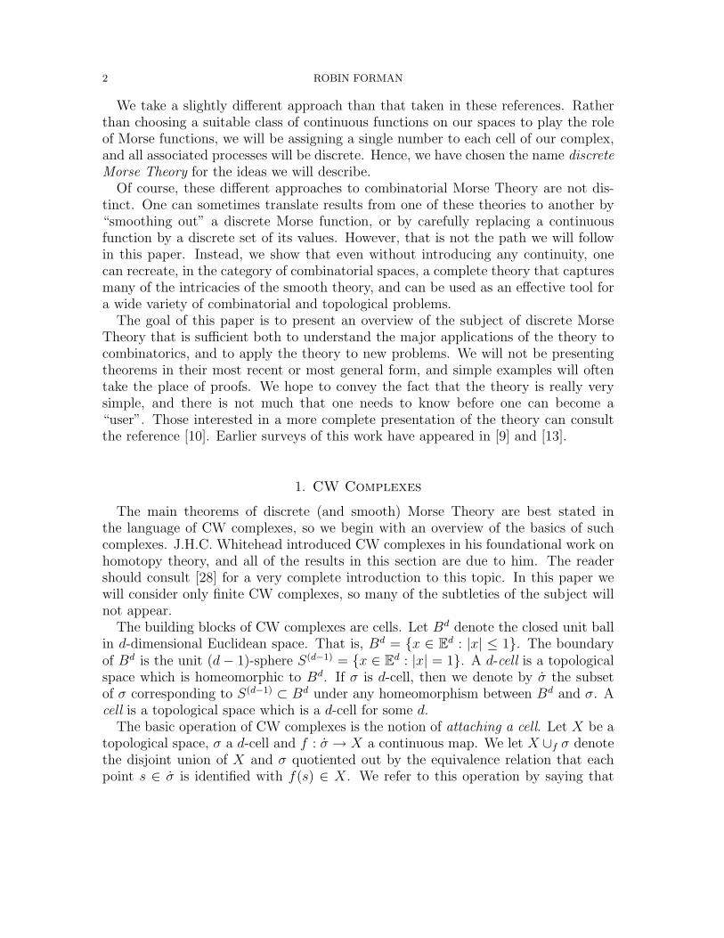
The building blocks of CW complexes are cells. Let Bd denote the closed unit ballin d-dimensional Euclidean space. That is, Bd = {x ∈ Ed : |x| ≤ 1}. The boundaryof Bd is the unit (d− 1)-sphere S(d−1) = {x ∈ Ed : |x| = 1}. A d-cell is a topologicalspace which is homeomorphic to Bd. If σ is d-cell, then we denote by σ the subsetof σ corresponding to S(d−1) ⊂ Bd under any homeomorphism between Bd and σ. Acell is a topological space which is a d-cell for some d.

The basic operation of CW complexes is the notion of attaching a cell. Let X be atopological space, σ a d-cell and f : σ → X a continuous map. We let X ∪f σ denotethe disjoint union of X and σ quotiented out by the equivalence relation that eachpoint s ∈ σ is identified with f(s) ∈ X. We refer to this operation by saying that

A USER’S GUIDE TO DISCRETE MORSE THEORY 3

X ∪f σ is the result of attaching the cell σ to X. The map f is called the attachingmap.

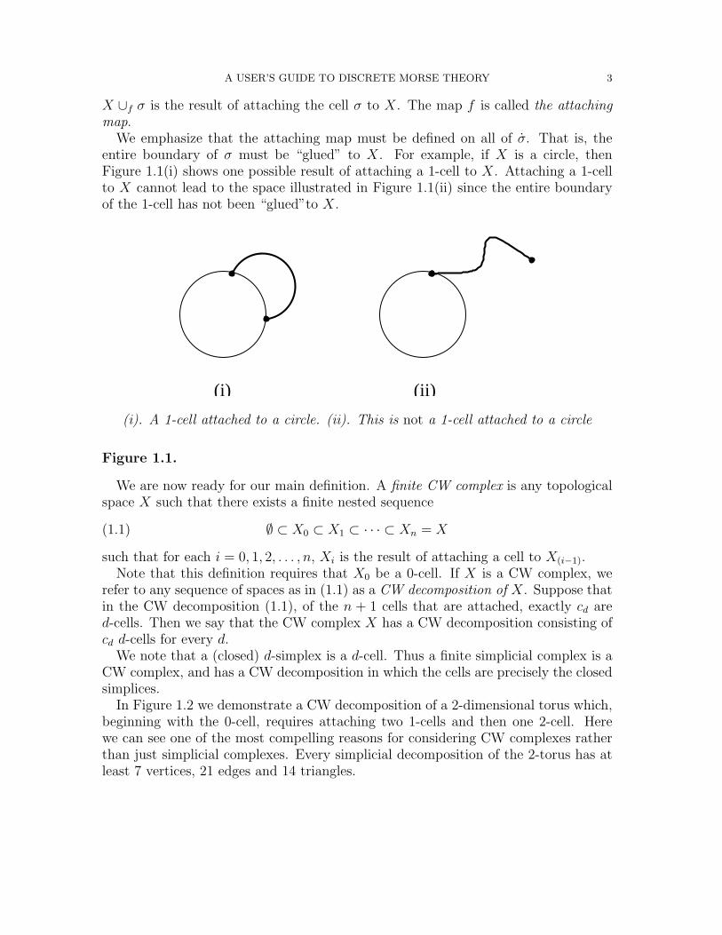
We emphasize that the attaching map must be defined on all of σ. That is, theentire boundary of σ must be “glued” to X. For example, if X is a circle, thenFigure 1.1(i) shows one possible result of attaching a 1-cell to X. Attaching a 1-cellto X cannot lead to the space illustrated in Figure 1.1(ii) since the entire boundaryof the 1-cell has not been “glued”to X.

(i) (ii)

(i). A 1-cell attached to a circle. (ii). This is not a 1-cell attached to a circle

Figure 1.1.

We are now ready for our main definition. A finite CW complex is any topologicalspace X such that there exists a finite nested sequence

(1.1) ∅ ⊂ X0 ⊂ X1 ⊂ · · · ⊂ Xn = X

such that for each i = 0, 1, 2, . . . , n, Xi is the result of attaching a cell to X(i−1).Note that this definition requires that X0 be a 0-cell. If X is a CW complex, we

refer to any sequence of spaces as in (1.1) as a CW decomposition of X. Suppose thatin the CW decomposition (1.1), of the n + 1 cells that are attached, exactly cd ared-cells. Then we say that the CW complex X has a CW decomposition consisting ofcd d-cells for every d.

We note that a (closed) d-simplex is a d-cell. Thus a finite simplicial complex is aCW complex, and has a CW decomposition in which the cells are precisely the closedsimplices.

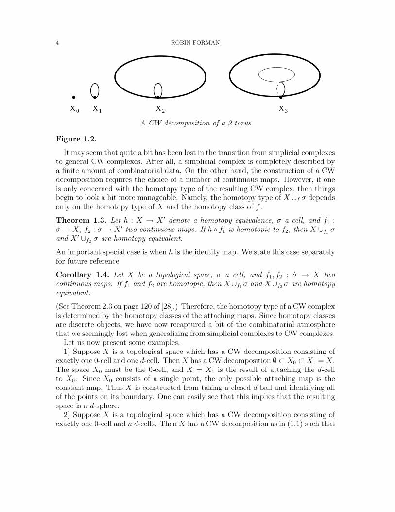
In Figure 1.2 we demonstrate a CW decomposition of a 2-dimensional torus which,beginning with the 0-cell, requires attaching two 1-cells and then one 2-cell. Herewe can see one of the most compelling reasons for considering CW complexes ratherthan just simplicial complexes. Every simplicial decomposition of the 2-torus has atleast 7 vertices, 21 edges and 14 triangles.

4 ROBIN FORMAN

X X X X0 1 2 3

A CW decomposition of a 2-torus

Figure 1.2.

It may seem that quite a bit has been lost in the transition from simplicial complexesto general CW complexes. After all, a simplicial complex is completely described bya finite amount of combinatorial data. On the other hand, the construction of a CWdecomposition requires the choice of a number of continuous maps. However, if oneis only concerned with the homotopy type of the resulting CW complex, then thingsbegin to look a bit more manageable. Namely, the homotopy type of X ∪f σ dependsonly on the homotopy type of X and the homotopy class of f .

Theorem 1.3. Let h : X → X ′ denote a homotopy equivalence, σ a cell, and f1 :σ → X, f2 : σ → X ′ two continuous maps. If h ◦ f1 is homotopic to f2, then X ∪f1 σand X ′ ∪f2 σ are homotopy equivalent.

An important special case is when h is the identity map. We state this case separatelyfor future reference.

Corollary 1.4. Let X be a topological space, σ a cell, and f1, f2 : σ → X twocontinuous maps. If f1 and f2 are homotopic, then X∪f1 σ and X∪f2 σ are homotopyequivalent.

(See Theorem 2.3 on page 120 of [28].) Therefore, the homotopy type of a CW complexis determined by the homotopy classes of the attaching maps. Since homotopy classesare discrete objects, we have now recaptured a bit of the combinatorial atmospherethat we seemingly lost when generalizing from simplicial complexes to CW complexes.

Let us now present some examples.1) Suppose X is a topological space which has a CW decomposition consisting of

exactly one 0-cell and one d-cell. Then X has a CW decomposition ∅ ⊂ X0 ⊂ X1 = X.The space X0 must be the 0-cell, and X = X1 is the result of attaching the d-cellto X0. Since X0 consists of a single point, the only possible attaching map is theconstant map. Thus X is constructed from taking a closed d-ball and identifying allof the points on its boundary. One can easily see that this implies that the resultingspace is a d-sphere.

2) Suppose X is a topological space which has a CW decomposition consisting ofexactly one 0-cell and n d-cells. Then X has a CW decomposition as in (1.1) such that


X0 is the 0-cell, and for each i = 1, 2, . . . , n the space Xi is the result of attaching a d-cell to X(i−1). From the previous example, we know that X1 is a d-sphere. The spaceX2 is constructed by attaching a d-cell to X1. The attaching map is a continuous mapfrom a (d− 1)-sphere to X1. Every map of the (d− 1)-sphere into X1 is homotopic toa constant map (since π(d−1)(X1) ∼= π(d−1)(S

d) ∼= 0). If the attaching map is actuallya constant map, then it is easy to see that the space X2 is the wedge of two d-spheres,denoted by Sd ∧ Sd. (The wedge of a collection of topological spaces is the spaceresulting from choosing a point in each space, taking the disjoint union of the spaces,and identifying all of the chosen points.) Since the attaching map must be homotopicto a constant map, Corollary 1.4 implies that X2 is homotopy equivalent to a wedgeof two d-spheres.

When constructing X3 by attaching a d-cell to X2, the relevant information is amap from Sd−1 to X2, and the homotopy type of the resulting space is determinedby the homotopy class of this map. All such maps are homotopic to a constant map(since πd−1(X2) ∼= πd−1(S

d ∧ Sd) ∼= 0). Since X2 is homotopy equivalent to a wedgeof two d-spheres, and the attaching map is homotopic to a constant map, it followsfrom Theorem 1.3 that X3 is homotopy equivalent to the space that would result fromattaching a d-cell to Sd ∧ Sd via a constant map, i.e., X3 is homotopy equivalent toa wedge of three d-spheres.

Continuing in this fashion, we can see that X must be homotopy equivalent to awedge of n d-spheres.

The reader should not get the impression that the homotopy type of a CW complexis determined by the number of cells of each dimension. This is true only for veryfew spaces (and the reader might enjoy coming up with some other examples). Thefact that wedges of spheres can, in fact, be identified by this numerical data partlyexplains why the main theorem of many papers in combinatorial topology is that acertain simplicial complex is homotopy equivalent to a wedge of spheres. Namelysuch complexes are the easiest to recognize. However, that does not explain why somany simplicial complexes that arise in combinatorics are homotopy equivalent to awedge of spheres. I have often wondered if perhaps there is some deeper explanationfor this.

3) Suppose that X is a CW complex which has a CW decomposition consistingof exactly one 0-cell, one 1-cell and one 2-cell. Let us consider a CW decompositionfor X with these cells: ∅ ⊂ X0 ⊂ X1 ⊂ X2 = X. We know that X0 is the 0-cell.Suppose that X1 is the result of attaching the 1-cell to X0. Then X1 must be a circle,and X2 arises from attaching a 2-cell to X1. The attaching map is a map from theboundary of the 2-cell, i.e., a circle, to X1 which is also a circle. Up to homotopy, sucha map is determined by its winding number, which can be taken to be a nonnegativeinteger. If the winding number is 0, then without altering the homotopy type ofX we may assume that the attaching map is a constant map, which yields thatX ∼ S1 ∧ S2 (where ∼ denotes homotopy equivalence). If the winding number is

6 ROBIN FORMAN

1 then without altering the homotopy type of X we may assume that the attachingmap is a homeomorphism, in which case X is a 2-dimensional disc. If the windingnumber is 2, then without altering the homotopy type of X we may assume that theattaching map is a standard degree 2 mapping (i.e., that wraps one circle aroundthe other twice, with no backtracking). The reader should convince him/herself thatthe result in this case is that X is the 2-dimensional projective space P2. In fact,each winding number results in a homotopically distinct space. These spaces can bedistinguished by their homology, since H1(X, Z) for the space X resulting from anattaching map with winding number n is isomorphic to Z/nZ.

It seems that we are not quite done with this example, because we assumed thatthe 1-cell was attached before the 2-cell, and we must consider the alternative order,in which X1 is the result of attaching a 2-cell to X0. In this case, X1 is a 2-sphere,and X = X2 is the result of attaching a 1-cell to X1. The attaching map is a mapof S0 into S2. Since S2 is connected (i.e., π0(S

2) = 0) all such maps are homotopicto a constant map. Taking the attaching map to be a constant map yields that X =S1 ∧ S2. Thus adding the cells in this order merely resulted in fewer possibilities forthe homotopy type of X. This is a general phenomenon. Generalizing the argumentwe just presented, using the fact that πi(S

d) = 0 for i < d, yields the followingstatement.

Theorem 1.5. Let

(1.2) ∅ ⊂ X0 ⊂ X2 ⊂ · · · ⊂ Xn = X

be a CW decomposition of a finite CW complex X. Then X is homotopy equivalent toa finite CW decomposition with precisely the same number of cells of each dimensionas in (1.2), and with the cells attached so that their dimensions form a nondecreasingsequence.

I first learned of simplicial complexes in an algebraic topology course. They wereintroduced as a category of topological spaces for which it was rather easy to definehomology and cohomology, i.e., in terms the simplicial chain- and cochain-complexes.One might be concerned that in the transition from simplicial complexes to CWcomplexes we have lost this ability to easily compute the homology. In fact, much ofthis computability remains. Let X be a CW complex with a fixed CW decomposition.Suppose that in this decomposition X is constructed from exactly cd cells of dimensiond for each d = 0, 1, 2, . . . , n = dim(K), and let Cd(X, Z) denote the space Zcd (moreprecisely, Cd(X, Z) denotes the free abelian group generated by the d-cells of X, eachendowed with an orientation). The following is one of the fundamental results in thetheory of CW complexes.

Theorem 1.6. There are boundary maps ∂d : Cd(X, Z) → Cd−1(X, Z), for each d, sothat

∂d−1 ◦ ∂d = 0


and such that the resulting differential complex

0 −→ Cn(X, Z)∂n−→ Cn−1(X, Z)

∂n−1−→ · · · ∂1−→ C0(X, Z) −→ 0

calculates the homology of X. That is, if we define

Hd(C, ∂) =Ker(∂d)

Im(∂d+1)

then for each dHd(C, ∂) ∼= Hd(X, Z)

where Hd(X, Z) denotes the singular homology of X.

The actual definition of the boundary map ∂ is slightly nontrivial and we will notgo into it here (see Ch. V Sec. 2 of [28] for the details). At first it may seem thatwithout knowing this boundary map, there is little to be gained from Theorem 1.6.In fact, much can be learned from just knowing of the existence of such a boundarymap. For example, let us choose a coefficient field F, and tensor everything with Fto get a differential complex

0 −→ Cn(X, F)∂n−→ Cn−1(X, F)

∂n−1−→ · · · ∂1−→ C0(X, F) −→ 0

which calculates H∗(X, F), where now Cd(X, F) ∼= Fcd . From basic linear algebra. wecan deduce the following inequalities.

Theorem 1.7. Let X be a CW complex with a fixed CW decomposition with cd cellsof dimension d for each d. Fix a coefficient field F and let b∗ denote the Betti numbersof X with respect to F, i.e., bd = dim(Hd(X, F)).(i) (The Weak Morse Inequalities) For each d

cd ≥ bd.

(ii) Let χ(X) denote the Euler characteristic of X, i.e.,

χ(X) = b0 − b1 + b2 − . . . .

then we also haveχ(X) = c0 − c1 + c2 − . . . .

As the name “Weak Morse Inequalities” implies, this theorem can be strengthened.The following inequalities, known as the “Strong Morse Inequalities” also follow fromstandard linear algebra.

Theorem 1.8 (The Strong Morse Inequalities). With all notation as in Theorem 1.7,for each d = 0, 1, 2, . . .

cd − cd−1 + cd−2 − · · ·+ (−1)dc0 ≥ bd − bd−1 + bd−2 − · · ·+ (−1)db0.

8 ROBIN FORMAN

Comparing Strong Morse Inequalities for consecutive values of d, and using the factthat bi = 0 for i larger than the dimension of K, yields Theorem 1.7.

We mentioned earlier that a great benefit of passing from simplicial complexes tothe more general CW complexes is that one often can use many fewer cells. Let ustake another look at this phenomenon in light of the Morse inequalities. Consider thecase where X is a two-dimensional torus, so that with respect to any coefficient fieldb0 = 1, b1 = 2, b2 = 1. From the weak Morse inequalities, we have that for any CWdecomposition,

c0 ≥ b0 = 1

c1 ≥ b1 = 2

c2 ≥ b2 = 1.

A simplicial decomposition is a special case of a CW decomposition, so these in-equalities are satisfied when cd denotes the number of d-simplices in a fixed simplicialdecomposition. However, every simplicial decomposition has at least 7 0-simplices,21 1-simplices and 14 2-simplices, so these inequalities are far from equality. It isgenerally the case that for a simplicial decomposition these inequalities are very farfrom optimal, and hence are generally of little interest. On the other hand, earlierwe demonstrated a CW decomposition of the two-torus with exactly one 0-cell, two1-cells and one 2-cell. The inequalities tell us, in particular, that one cannot build atwo-torus using fewer cells.

2. The Basics of Discrete Morse Theory

The discussion in the previous section leads us to an important question. Supposeone is given a finite simplicial complex X. Typically, we can expect that X has a CWdecomposition with many fewer cells than in the original simplicial decomposition.How can one go about finding such an “efficient” CW decomposition for X? In thissection we present a technique, discrete Morse Theory, which can be useful in suchan investigation. (We note that the ideas we will describe can be applied with nomodification at all to any finite regular CW complex, and with only minor modifica-tions to a general finite CW complex. However, for simplicity, in this paper we willrestrict attention to simplicial complexes.)

We begin by recalling that a finite simplicial complex is a finite set of vertices V ,along with a set of subsets K of V . The set K satisfies two main properties:1) V ⊆ K2) If α ∈ K and β ⊆ α then β ∈ K.By a slight abuse of notation, we will refer to the simplicial complex simply as K.The elements of K are called simplices. If α ∈ K, and α contains p + 1 vertices,then we say that the dimension of α is p, and we will sometimes denote this by α(p).For simplices α and β we will use the notation α < β or β > α to indicate that αis a proper subset of β (thinking of α and β as subsets of V ), and say that α is a


face of β. We emphasize that at this point we will not be placing any restrictions onthe finite simplicial complexes under investigation. In particular, the complexes neednot be manifolds (even though many of our examples will be). In Section 9 we willbriefly indicate how some of our conclusions can be strengthened in the case that thecomplexes are assumed to have additional structure.

A discrete Morse function on K is a function which, roughly speaking, assignshigher numbers to higher dimensional simplices, with at most one exception, locally,at each simplex. More precisely,

Definition 2.1. A function

f : K −→ Ris a discrete Morse function if for every α(p) ∈ K

(1) #{β(p+1) > α | f(β) ≤ f(α)} ≤ 1,

and

(2) #{γ(p−1) < α | f(γ) ≥ f(α)} ≤ 1.

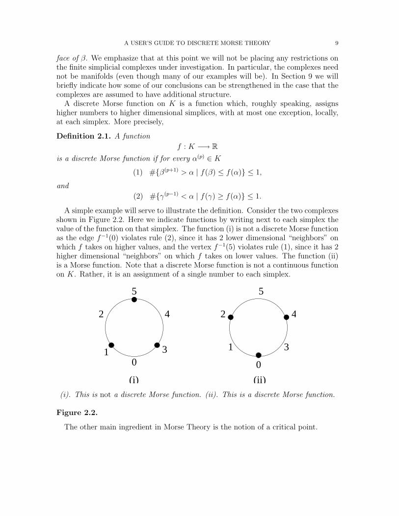
A simple example will serve to illustrate the definition. Consider the two complexesshown in Figure 2.2. Here we indicate functions by writing next to each simplex thevalue of the function on that simplex. The function (i) is not a discrete Morse functionas the edge f−1(0) violates rule (2), since it has 2 lower dimensional “neighbors” onwhich f takes on higher values, and the vertex f−1(5) violates rule (1), since it has 2higher dimensional “neighbors” on which f takes on lower values. The function (ii)is a Morse function. Note that a discrete Morse function is not a continuous functionon K. Rather, it is an assignment of a single number to each simplex.

5

4

3

4

5

3 0

1 1

2

(i) (ii)

2

0

(i). This is not a discrete Morse function. (ii). This is a discrete Morse function.

Figure 2.2.

The other main ingredient in Morse Theory is the notion of a critical point.

10 ROBIN FORMAN

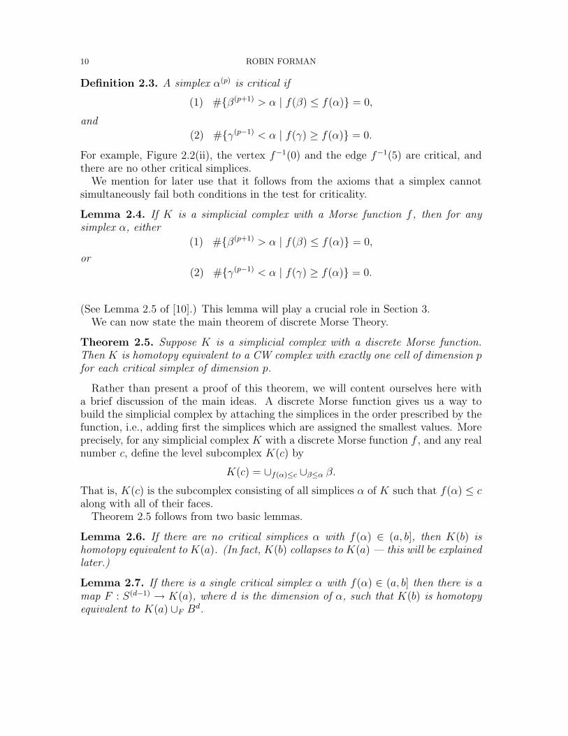
Definition 2.3. A simplex α(p) is critical if

(1) #{β(p+1) > α | f(β) ≤ f(α)} = 0,

and

(2) #{γ(p−1) < α | f(γ) ≥ f(α)} = 0.

For example, Figure 2.2(ii), the vertex f−1(0) and the edge f−1(5) are critical, andthere are no other critical simplices.

We mention for later use that it follows from the axioms that a simplex cannotsimultaneously fail both conditions in the test for criticality.

Lemma 2.4. If K is a simplicial complex with a Morse function f , then for anysimplex α, either

(1) #{β(p+1) > α | f(β) ≤ f(α)} = 0,

or

(2) #{γ(p−1) < α | f(γ) ≥ f(α)} = 0.

(See Lemma 2.5 of [10].) This lemma will play a crucial role in Section 3.We can now state the main theorem of discrete Morse Theory.

Theorem 2.5. Suppose K is a simplicial complex with a discrete Morse function.Then K is homotopy equivalent to a CW complex with exactly one cell of dimension pfor each critical simplex of dimension p.

Rather than present a proof of this theorem, we will content ourselves here witha brief discussion of the main ideas. A discrete Morse function gives us a way tobuild the simplicial complex by attaching the simplices in the order prescribed by thefunction, i.e., adding first the simplices which are assigned the smallest values. Moreprecisely, for any simplicial complex K with a discrete Morse function f , and any realnumber c, define the level subcomplex K(c) by

K(c) = ∪f(α)≤c ∪β≤α β.

That is, K(c) is the subcomplex consisting of all simplices α of K such that f(α) ≤ calong with all of their faces.

Theorem 2.5 follows from two basic lemmas.

Lemma 2.6. If there are no critical simplices α with f(α) ∈ (a, b], then K(b) ishomotopy equivalent to K(a). (In fact, K(b) collapses to K(a) — this will be explainedlater.)

Lemma 2.7. If there is a single critical simplex α with f(α) ∈ (a, b] then there is amap F : S(d−1) → K(a), where d is the dimension of α, such that K(b) is homotopyequivalent to K(a) ∪F Bd.


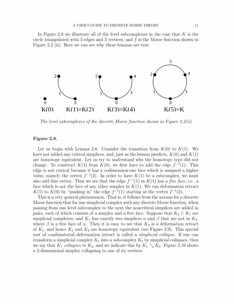
In Figure 2.8 we illustrate all of the level subcomplexes in the case that K is thecircle triangulated with 3 edges and 3 vertices, and f is the Morse function shown inFigure 2.2 (ii). Here we can see why these lemmas are true.

0

1

2

3

4

5

0 0 0

1 1

2 2

3

4

K(1)=K(2)K(0) K(3)=K(4) K(5)=K

The level subcomplexes of the discrete Morse function shown in Figure 2.2(ii)

Figure 2.8.

Let us begin with Lemma 2.6. Consider the transition from K(0) to K(1). Wehave not added any critical simplices, and, just as the lemma predicts, K(0) and K(1)are homotopy equivalent. Let us try to understand why the homotopy type did notchange. To construct K(1) from K(0), we first have to add the edge f−1(1). Thisedge is not critical because it has a codimension-one face which is assigned a highervalue, namely the vertex f−1(2). In order to have K(1) be a subcomplex, we mustalso add this vertex. Thus we see that the edge f−1(1) in K(1) has a free face, i.e., aface which is not the face of any other simplex in K(1). We can deformation retractK(1) to K(0) by “pushing in” the edge f−1(1) starting at the vertex f−1(2).

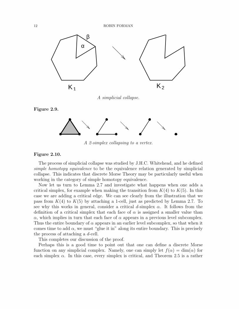
This is a very general phenomenon. That is, it follows from the axioms for a discreteMorse function that for any simplicial complex with any discrete Morse function, whenpassing from one level subcomplex to the next the noncritical simplices are added inpairs, each of which consists of a simplex and a free face. Suppose that K2 ⊂ K1 aresimplicial complexes, and K1 has exactly two simplices α and β that are not in K2,where β is a free face of α. Then it is easy to see that K2 is a deformation retractof K1, and hence K1 and K2 are homotopy equivalent (see Figure 2.9). This specialsort of combinatorial deformation retract is called a simplicial collapse. If one cantransform a simplicial complex K1 into a subcomplex K2 by simplicial collapses, thenwe say that K1 collapses to K2, and we indicate this by K1 ↘ K2. Figure 2.10 showsa 2-dimensional simplex collapsing to one of its vertices.

12 ROBIN FORMAN

Κ Κ

αβ

1 2

A simplicial collapse.

Figure 2.9.

A 2-simplex collapsing to a vertex.

Figure 2.10.

The process of simplicial collapse was studied by J.H.C. Whitehead, and he definedsimple homotopy equivalence to be the equivalence relation generated by simplicialcollapse. This indicates that discrete Morse Theory may be particularly useful whenworking in the category of simple homotopy equivalence.

Now let us turn to Lemma 2.7 and investigate what happens when one adds acritical simplex, for example when making the transition from K(4) to K(5). In thiscase we are adding a critical edge. We can see clearly from the illustration that wepass from K(4) to K(5) by attaching a 1-cell, just as predicted by Lemma 2.7. Tosee why this works in general, consider a critical d-simplex α. It follows from thedefinition of a critical simplex that each face of α is assigned a smaller value thanα, which implies in turn that each face of α appears in a previous level subcomplex.Thus the entire boundary of α appears in an earlier level subcomplex, so that when itcomes time to add α, we must “glue it in” along its entire boundary. This is preciselythe process of attaching a d-cell.

This completes our discussion of the proof.Perhaps this is a good time to point out that one can define a discrete Morse

function on any simplicial complex. Namely, one can simply let f(α) = dim(α) foreach simplex α. In this case, every simplex is critical, and Theorem 2.5 is a rather


uninteresting tautology. However, as we will see in examples, one can often constructdiscrete Morse functions with many fewer critical simplices.

Let K be a simplicial complex with a discrete Morse function. Let mp denote thenumber of critical simplices of dimension p. Let F be any field, and bp = dim Hp(K, F)the pth Betti number with respect to F. Combining Theorems 2.5, 1.7 and 1.8, andthe fact that homotopy equivalent spaces have isomorphic homology, we have thefollowing inequalities.

Theorem 2.11. I. The Weak Morse Inequalities.(i)For each p = 0, 1, 2, . . . , n (where n is the dimension of K)

mp ≥ bp.

(ii) m0 −m1 + m2 − · · ·+ (−1)nmn = b0 − b1 + b2 − · · ·+ (−1)nbn [= χ(K)].

II. The Strong Morse Inequalities.For each p = 0, 1, 2, . . . , n, n + 1,

mp −mp−1 + · · ·+ (−1)pm0 ≥ bp − bp−1 + · · ·+ (−1)pb0.

3. Gradient Vector Fields

Any ambitious reader who has already started trying some examples will havenoticed that the theory as presented in the previous section can be a bit unwieldy.After all, how is one to go about assigning numbers to each of the simplices of asimplicial complex so that they satisfy the axioms of a discrete Morse function?Fortunately, in practice one need not actually find a discrete Morse function. Findingthe gradient vector field of the Morse function is sufficient. This requires a bit ofexplanation.

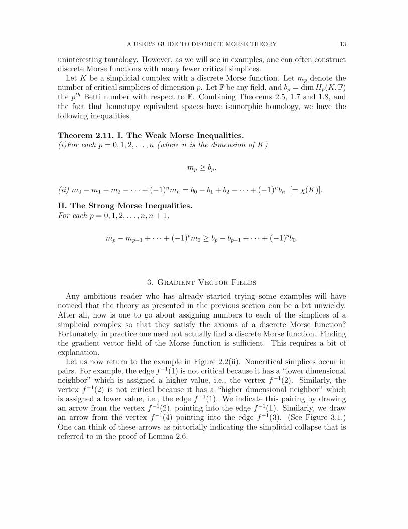
Let us now return to the example in Figure 2.2(ii). Noncritical simplices occur inpairs. For example, the edge f−1(1) is not critical because it has a “lower dimensionalneighbor” which is assigned a higher value, i.e., the vertex f−1(2). Similarly, thevertex f−1(2) is not critical because it has a “higher dimensional neighbor” whichis assigned a lower value, i.e., the edge f−1(1). We indicate this pairing by drawingan arrow from the vertex f−1(2), pointing into the edge f−1(1). Similarly, we drawan arrow from the vertex f−1(4) pointing into the edge f−1(3). (See Figure 3.1.)One can think of these arrows as pictorially indicating the simplicial collapse that isreferred to in the proof of Lemma 2.6.

14 ROBIN FORMAN

0

2 4

5

1 3

The gradient vector field of the Morse function shown in Figure 2.2 (ii).

Figure 3.1.

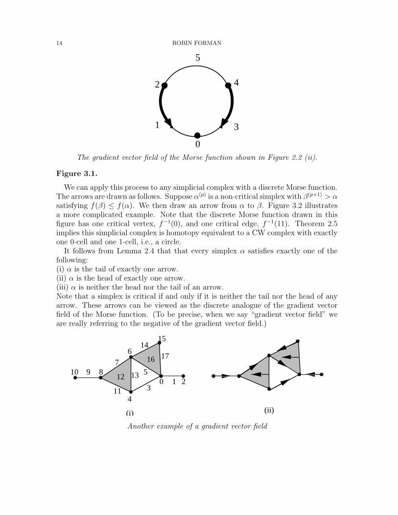
We can apply this process to any simplicial complex with a discrete Morse function.The arrows are drawn as follows. Suppose α(p) is a non-critical simplex with β(p+1) > αsatisfying f(β) ≤ f(α). We then draw an arrow from α to β. Figure 3.2 illustratesa more complicated example. Note that the discrete Morse function drawn in thisfigure has one critical vertex, f−1(0), and one critical edge, f−1(11). Theorem 2.5implies this simplicial complex is homotopy equivalent to a CW complex with exactlyone 0-cell and one 1-cell, i.e., a circle.

It follows from Lemma 2.4 that that every simplex α satisfies exactly one of thefollowing:(i) α is the tail of exactly one arrow.(ii) α is the head of exactly one arrow.(iii) α is neither the head nor the tail of an arrow.Note that a simplex is critical if and only if it is neither the tail nor the head of anyarrow. These arrows can be viewed as the discrete analogue of the gradient vectorfield of the Morse function. (To be precise, when we say “gradient vector field” weare really referring to the negative of the gradient vector field.)

11

513

17

1514

910 87

6

4

3210

(ii)(i)

16

12

Another example of a gradient vector field


Figure 3.2.

As we will see in examples later, these arrows are much easier to work with thanthe original discrete Morse function. In fact, this gradient vector field contains all ofthe information that we will need to know about the function for most applications.The upshot is that if one is given a simplicial complex and one wishes to apply thetheory of the previous section, one need not find a discrete Morse function. One“only” needs to find a gradient vector field.

This leads us to the following question. Suppose we attach arrows to the simplicesso that each simplex satisfies exactly one of properties (i),(ii),(iii) above. Then how dowe know if that set of arrows is the gradient vector field of a discrete Morse function?This is the question we will answer in the remainder of this section.

Let K be a simplicial complex with a discrete Morse function f . Then rather thanthinking about the discrete gradient vector field V of f as a collection of arrows,we may equivalently describe V as a collection of pairs {α(p) < β(p+1)} of simplicesof K, where {α(p) < β(p+1)} is in V if and only if f(β) ≤ f(α). In other words,{α(p) < β(p+1)} is in V if and only if we have drawn an arrow that has α as itstail, and β as its head. The properties of a discrete Morse function imply that eachsimplex is in at most one pair of V . This leads us to the following definition.

Definition 3.3. A discrete vector field V on K is a collection of pairs {α(p) < β(p+1)}of simplices of K such that each simplex is in at most one pair of V .

Such pairings were studied in [41] and [8] as a tool for investigating the possiblef -vectors for a simplicial complex. Here we take a different point of view. If onehas a smooth vector field on a smooth manifold, it is quite natural to study thedynamical system induced by flowing along the vector field. One can begin the samesort of study for any discrete vector field. In [12] we present a study of the dynamicsassociated to a discrete vector field. Here, we present just enough to continue ourdiscussion of discrete Morse Theory.

Given a discrete vector field V on a simplicial complex K, a V−path is a sequenceof simplices

(3.1) α(p)0 , β

(p+1)0 , α

(p)1 , β

(p+1)1 , α

(p)2 , . . . , β(p+1)

r , α(p)r+1

such that for each i = 0, . . . r, {α < β} ∈ V and βi > αi+1 6= αi. We say such a pathis a non-trivial closed path if r ≥ 0 and α0 = αr+1. If V is the gradient vector field ofa discrete Morse function f , then we sometimes refer to a V -path as a gradient pathof f .

One idea behind this definition is the following result.

Theorem 3.4. Suppose V is the gradient vector field of a discrete Morse function f .Then a sequence of simplices as in (3.1) is a V -path if and only if αi < βi > αi+1 foreach i = 0, 1, . . . , r, and

f(α0) ≥ f(β0) > f(α1) ≥ f(β1) > · · · ≥ f(βr) > f(αr+1).

16 ROBIN FORMAN

That is, the gradient paths of f are precisely those “continuous” sequences of simplicesalong which f is decreasing. In particular, this theorem implies that if V is a gradientvector field, then there are no nontrivial closed V -paths. In fact, the main result ofthis section is that the converse is true.

Theorem 3.5. A discrete vector field V is the gradient vector field of a discreteMorse function if and only if there are no non-trivial closed V -paths.

We will not prove this theorem here. However, many readers may notice the simi-larity with the following standard theorem from the subject of directed graphs.

Theorem 3.6. Let G be a directed graph. Then there is a real-valued function of thevertices that is strictly decreasing along each directed path if and only if there are nodirected loops.

We will show in Section 6 that, in fact, Theorem 3.6 implies Theorem 3.5. Thepower of Theorem 3.5 is indicated in the next two sections in which we construct somediscrete vector fields and use Theorem 3.5 to verify that they are gradient vector fields.

4. Our First Example: The Real Projective Plane

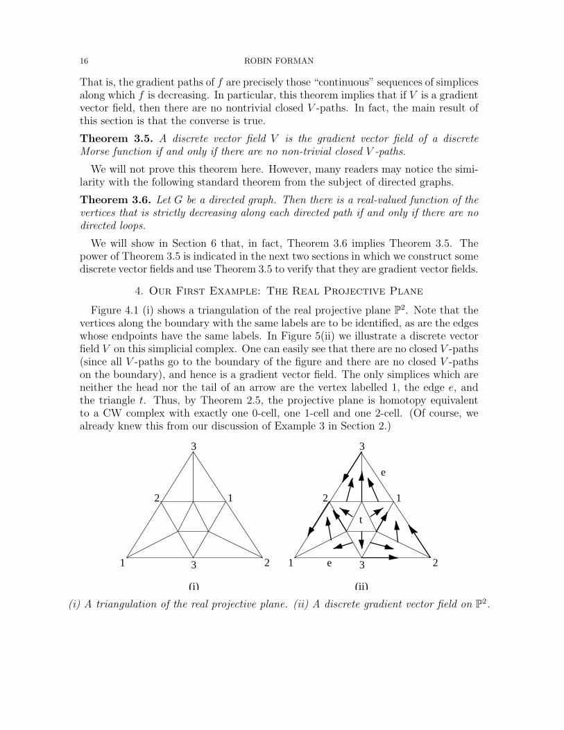
Figure 4.1 (i) shows a triangulation of the real projective plane P2. Note that thevertices along the boundary with the same labels are to be identified, as are the edgeswhose endpoints have the same labels. In Figure 5(ii) we illustrate a discrete vectorfield V on this simplicial complex. One can easily see that there are no closed V -paths(since all V -paths go to the boundary of the figure and there are no closed V -pathson the boundary), and hence is a gradient vector field. The only simplices which areneither the head nor the tail of an arrow are the vertex labelled 1, the edge e, andthe triangle t. Thus, by Theorem 2.5, the projective plane is homotopy equivalentto a CW complex with exactly one 0-cell, one 1-cell and one 2-cell. (Of course, wealready knew this from our discussion of Example 3 in Section 2.)

2

3

1

1 23

t

e

e

2

3

1

1 23

(i) (ii)

(i) A triangulation of the real projective plane. (ii) A discrete gradient vector field on P2.


Figure 4.1.

This example gives rise to two potential concerns. The first is that from the maintheorem we learn only a statement about “homotopy equivalence”. This is sufficientif one is only interested in calculating homology or homotopy groups. However, onemight be interested in determining the (PL-)homeomorphism type of the complex.This is possible, in some cases, using deep results of J.H.C. Whitehead. We revisitthis topic in Section 8.

The second potential point of concern is that as we saw in Section 2 there are aninfinite number of different homotopy types of CW complexes which can be built fromexactly one 0-cell, one 1-cell and one 2-cell. One might wonder if Morse Theory cangive us any additional information as to how the cells are attached. In fact, one candeduce much of this information if one has enough information about the gradientpaths of the Morse function. This point is discussed further in Section 7, where wewill return to this example of the triangulated projective plane.

5. Our Second Example: The Complex of Not Connected Graphs

A number of fascinating simplicial complexes arise from the study of monotonegraph properties. Let Kn denote the complete graph on n vertices, and suppose wehave labelled the vertices 1,2,. . . ,n. Let Gn denote the spanning subgraphs of Kn, thatis, the subgraphs of Kn that contain all n vertices. A subset P ⊂ Gn is called a graphproperty of graphs with n vertices if inclusion in P only depends on the isomorphismtype of the graph. That is, P is a graph property if for all pairs of graphs G1, G2 ∈ Gn,if G1 and G2 are isomorphic (ignoring the labellings on the vertices) then G1 ∈ Pif and only if G2 ∈ P . A graph property P of graphs with n vertices is said to bemonotone decreasing if for any graphs G1 ⊂ G2 ∈ Gn, if G2 ∈ P then G1 ∈ P .

Monotone decreasing properties abound in the study of graph theory. Here aresome typical examples: graphs having no more than k edges (for any fixed k), graphssuch that the degree of every vertex is less that δ (for any fixed δ), graphs which arenot connected, graphs which are not i-connected (for any fixed i), graphs which donot have a Hamiltonian cycle, graphs which do not contain a minor isomorphic to H(for any fixed graph H), graphs which are r-colorable (for any fixed r), and bipartitegraphs.

Any monotone decreasing graph property P gives rise to a simplicial complex Kwhere the d-simplices of K are the graphs G ∈ P which have d+1 edges. In particular,if G is a d-simplex inK, then the faces of G are all of the nontrivial spanning subgraphsof G (the monotonicity of P implies that each of these graphs is in K). Said in anotherway, if P is nonempty, then the vertices of K are the edges of Kn, and a collection ofvertices in K span a simplex if the spanning subgraph of Kn consisting of all edgeswhich correspond to these vertices lies in P .

The simplicial complexes induced by many of the above-mentioned monotone de-creasing graph properties have been studied using the techniques of this paper. See

18 ROBIN FORMAN

for example [6], [7], [21], [22], [27], [37]. These papers contain some beautiful math-ematics in which the authors construct, “by hand”, explicit discrete gradient vectorfields, along the way illuminating some of the intricate finer structures of the graphproperties.

Some monotone graph properties have recently been the focus of intense interestbecause of their relation to knot theory. Unfortunately this is probably not a goodtime for an in depth discussion of this fascinating topic. We will mention only thatVassiliev has shown how one can derive “finite type knot invariants” from the studyof the space of “singular knots” (i.e., maps from S1 to R3 which are not embeddings).The homology of the simplicial complexes of not connected and not 2-connectedgraphs show up in his spectral sequence calculation of the homology of this space.This is explained in [43], where Vassiliev derives the homotopy type of the complexof not connected graphs. In [42] and [1], the topology of the space of not 2-connectedgraphs is determined, with discrete Morse Theory playing a minor role in the latterreference. This topic is reexamined in [37], in which the entire investigation is framedin the language of discrete Morse Theory. Discrete Morse Theory is used to determinethe topology of not 3-connected graphs in [21].

In this section, we will provide an introduction to this work by taking a look at thesimpler case of the complex of not connected graphs. We will show how the ideas ofthis paper may be used to determine the topology of Nn, the simplicial complex ofnot connected graphs on n vertices. Let me begin by pointing out that this complexcan be well studied by more classical methods, and the answer has also been found byVassiliev in [43]. The only novelty of this section is our use of discrete Morse Theory.

Our goal is to construct a discrete gradient vector field V on Nn, the simplicialcomplex of all not-connected graphs with the vertex set {1, 2, 3, . . . , n}. The con-struction will be in steps. Let V12 denote the discrete vector field consisting of allpairs {G, G + (1, 2)}, where G is any graph in Nn which does not contain the edge(1, 2) and such that G + (1, 2) ∈ Nn. Another way of describing V12 is that if G isany graph in Nn which contains the edge (1, 2), then G− (1, 2) and G are paired inV12. Actually, there is one exception to this rule. Let G∗ denote the graph consistingof only the single edge (1,2). Then G∗− (1, 2) is the empty graph, which correspondsto the empty simplex in Nn, and may not be paired in a discrete vector field. Thus,G∗ is unpaired in V12.

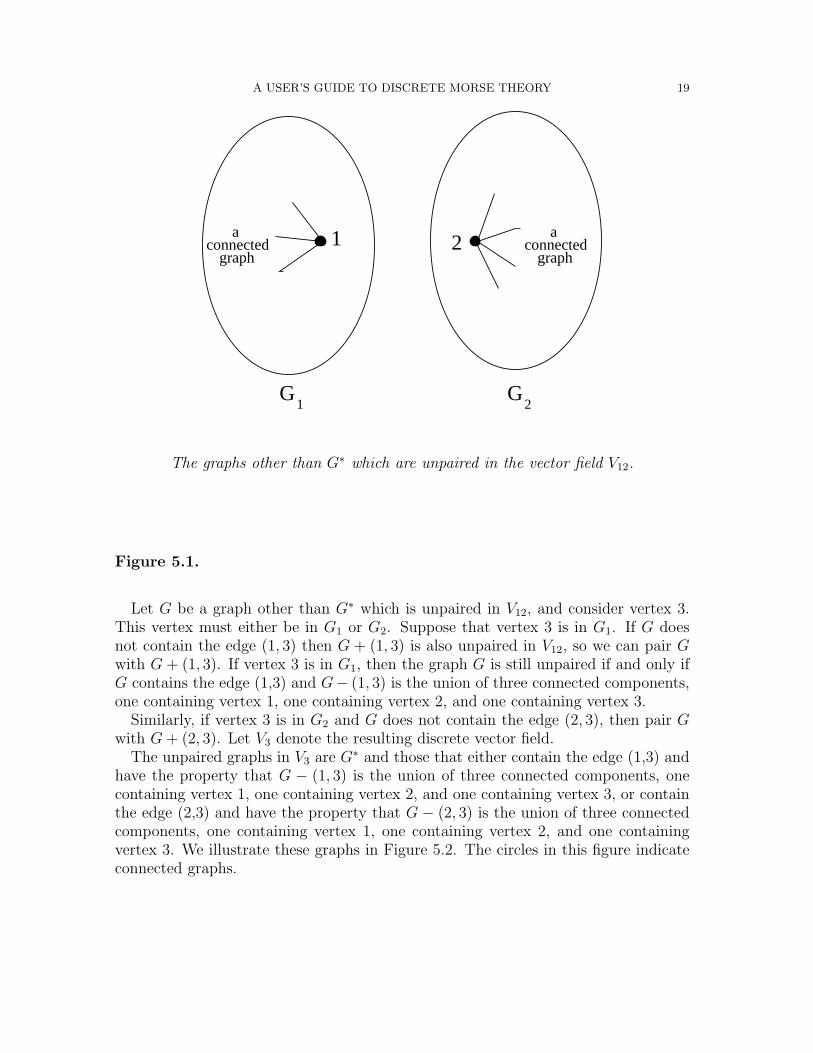
The graphs in Nn other than G∗ which are unpaired in V12 are those that donot contain the edge (1, 2) and have the property that G + (1, 2) 6∈ Nn. That is,those disconnected graphs G with the property that G + (1, 2) is connected. Such agraph must have exactly two connected components, one of which contains the vertexlabelled 1, and one which contains the vertex labelled 2. We denote these connectedcomponents by G1 and G2, resp. See Figure 5.1.


1 2

G1

G2

connecteda

graph graphconnected

a

The graphs other than G∗ which are unpaired in the vector field V12.

Figure 5.1.

Let G be a graph other than G∗ which is unpaired in V12, and consider vertex 3.This vertex must either be in G1 or G2. Suppose that vertex 3 is in G1. If G doesnot contain the edge (1, 3) then G + (1, 3) is also unpaired in V12, so we can pair Gwith G + (1, 3). If vertex 3 is in G1, then the graph G is still unpaired if and only ifG contains the edge (1,3) and G− (1, 3) is the union of three connected components,one containing vertex 1, one containing vertex 2, and one containing vertex 3.

Similarly, if vertex 3 is in G2 and G does not contain the edge (2, 3), then pair Gwith G + (2, 3). Let V3 denote the resulting discrete vector field.

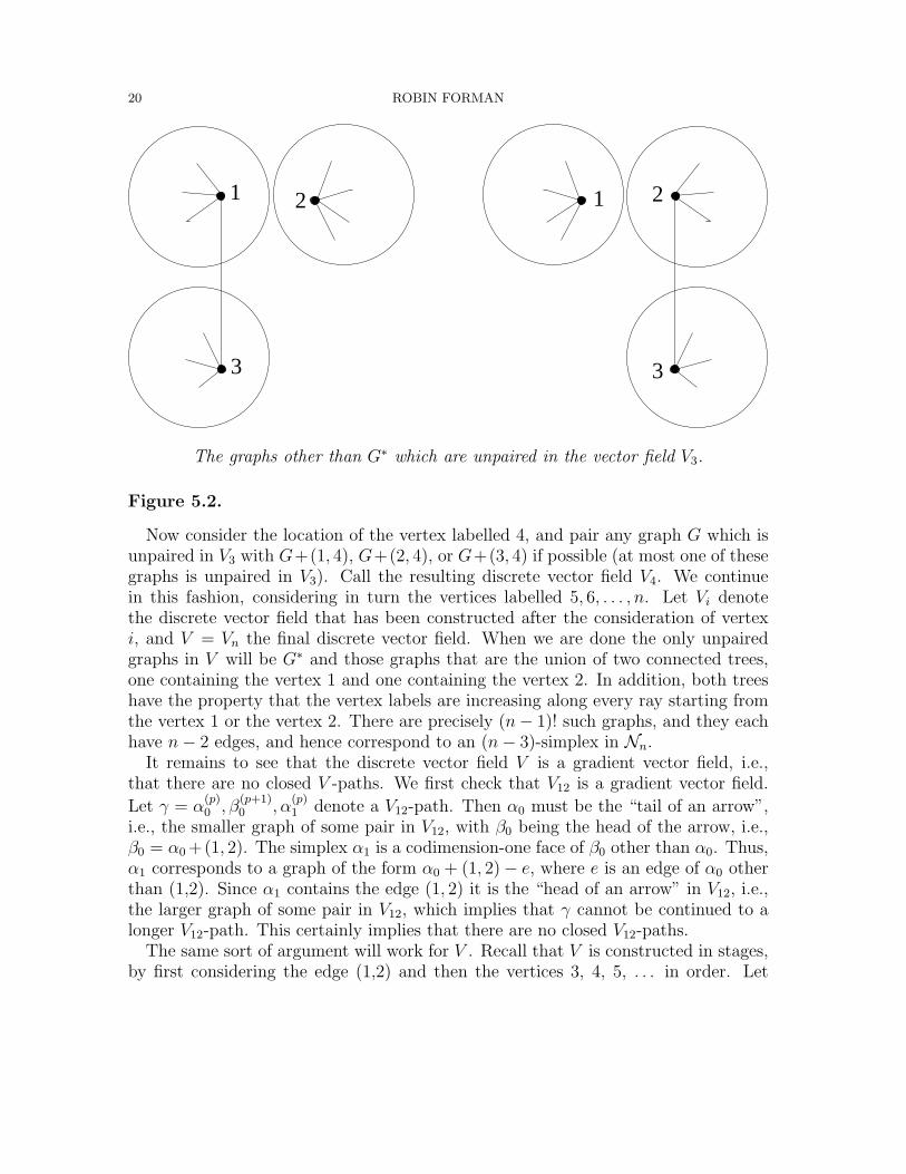
The unpaired graphs in V3 are G∗ and those that either contain the edge (1,3) andhave the property that G − (1, 3) is the union of three connected components, onecontaining vertex 1, one containing vertex 2, and one containing vertex 3, or containthe edge (2,3) and have the property that G− (2, 3) is the union of three connectedcomponents, one containing vertex 1, one containing vertex 2, and one containingvertex 3. We illustrate these graphs in Figure 5.2. The circles in this figure indicateconnected graphs.

20 ROBIN FORMAN

3

21

3

1 2

The graphs other than G∗ which are unpaired in the vector field V3.

Figure 5.2.

Now consider the location of the vertex labelled 4, and pair any graph G which isunpaired in V3 with G+(1, 4), G+(2, 4), or G+(3, 4) if possible (at most one of thesegraphs is unpaired in V3). Call the resulting discrete vector field V4. We continuein this fashion, considering in turn the vertices labelled 5, 6, . . . , n. Let Vi denotethe discrete vector field that has been constructed after the consideration of vertexi, and V = Vn the final discrete vector field. When we are done the only unpairedgraphs in V will be G∗ and those graphs that are the union of two connected trees,one containing the vertex 1 and one containing the vertex 2. In addition, both treeshave the property that the vertex labels are increasing along every ray starting fromthe vertex 1 or the vertex 2. There are precisely (n− 1)! such graphs, and they eachhave n− 2 edges, and hence correspond to an (n− 3)-simplex in Nn.

It remains to see that the discrete vector field V is a gradient vector field, i.e.,that there are no closed V -paths. We first check that V12 is a gradient vector field.

Let γ = α(p)0 , β

(p+1)0 , α

(p)1 denote a V12-path. Then α0 must be the “tail of an arrow”,

i.e., the smaller graph of some pair in V12, with β0 being the head of the arrow, i.e.,β0 = α0 +(1, 2). The simplex α1 is a codimension-one face of β0 other than α0. Thus,α1 corresponds to a graph of the form α0 + (1, 2)− e, where e is an edge of α0 otherthan (1,2). Since α1 contains the edge (1, 2) it is the “head of an arrow” in V12, i.e.,the larger graph of some pair in V12, which implies that γ cannot be continued to alonger V12-path. This certainly implies that there are no closed V12-paths.

The same sort of argument will work for V . Recall that V is constructed in stages,by first considering the edge (1,2) and then the vertices 3, 4, 5, . . . in order. Let


γ = α0, β0, α1 denote a V -path. In particular, α0 and β0 must be paired in V . Thereader can check that if α0 and β0 are first paired in Vi, i ≥ 3, then either α1 is thehead of an arrow in Vi, in which case the V -path cannot be continued, or α1 is pairedin Vi−1. It follows by induction that there can be no closed V -paths.

In summary, V is a discrete gradient vector field on Nn with exactly one unpairedvertex, and (n − 1)! unpaired (n − 3)-simplices. We can now apply Theorem 2.5 toconclude

Theorem 5.3 ([43]). The complex Nn of not connected graphs on n-vertices is ho-motopy equivalent to the wedge of (n− 1)! spheres of dimension (n− 3).

6. A Combinatorial Point of View

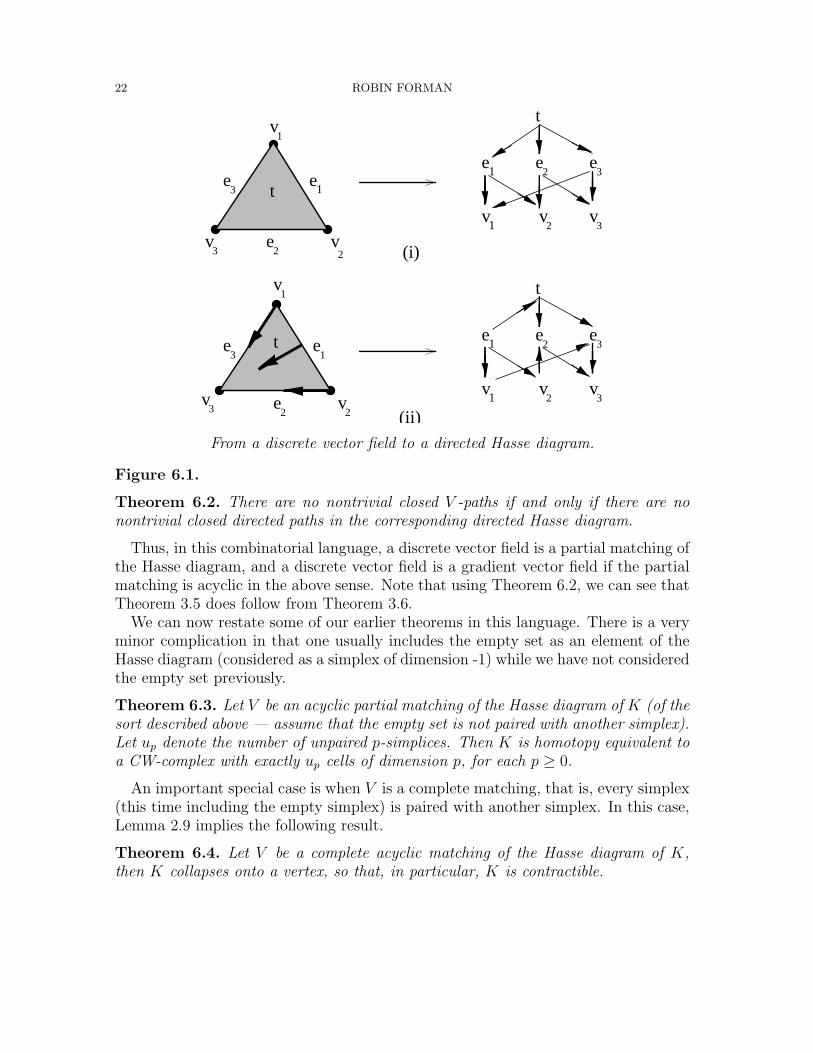
The notion of a gradient vector field has a very nice purely combinatorial descriptiondue to Chari [6], using which we can recast the Morse Theory in an appealing form.We begin with the Hasse diagram of K, that is, the partially ordered set of simplicesof K ordered by the face relation. Consider the Hasse diagram as a directed graph.The vertices of the graph are in 1-1 correspondence with the simplices of K, and thereis a directed edge from β to α if and only if α is a codimension-one face of β. (SeeFigure 6.1 (i).) Now let V be a combinatorial vector field. We modify the directedgraph as follows. If {α < β} ∈ V then reverse the orientation of the edge between αand β, so that it now goes from α to β. (See Figure 6.1(ii).) A V -path can be thoughtof as a directed path in this modified graph. There are some directed paths in thismodified Hasse diagram which are not V -paths as we have defined them. However,the following result is not hard to check.

22 ROBIN FORMAN

v

v

v

v

e

e

e

e

t

1

3

1

3

1

1e

2

2

3

e3

v2

v2

e

v

ee

v v

t

1 2

3

3

21

e

v

ee

v v

t

1 2

3

3

21t

(i)

(ii)From a discrete vector field to a directed Hasse diagram.

Figure 6.1.

Theorem 6.2. There are no nontrivial closed V -paths if and only if there are nonontrivial closed directed paths in the corresponding directed Hasse diagram.

Thus, in this combinatorial language, a discrete vector field is a partial matching ofthe Hasse diagram, and a discrete vector field is a gradient vector field if the partialmatching is acyclic in the above sense. Note that using Theorem 6.2, we can see thatTheorem 3.5 does follow from Theorem 3.6.

We can now restate some of our earlier theorems in this language. There is a veryminor complication in that one usually includes the empty set as an element of theHasse diagram (considered as a simplex of dimension -1) while we have not consideredthe empty set previously.

Theorem 6.3. Let V be an acyclic partial matching of the Hasse diagram of K (of thesort described above — assume that the empty set is not paired with another simplex).Let up denote the number of unpaired p-simplices. Then K is homotopy equivalent toa CW-complex with exactly up cells of dimension p, for each p ≥ 0.

An important special case is when V is a complete matching, that is, every simplex(this time including the empty simplex) is paired with another simplex. In this case,Lemma 2.9 implies the following result.

Theorem 6.4. Let V be a complete acyclic matching of the Hasse diagram of K,then K collapses onto a vertex, so that, in particular, K is contractible.


This result was used in a very interesting fashion in [1].

7. The Morse Complex

In this section we will see how knowledge of the gradient paths of a discrete Morsefunction on a space K can allow one to strengthen the conclusions of the main theo-rems. In particular, rather than just knowing the number of cells in a CW decompo-sition for K, one can calculate the homology exactly.

Let K be a simplicial complex with a Morse function f . Let Cp(X, Z) denote thespace of p-simplicial chains, and Mp ⊆ Cp(X, Z) the span of the critical p-simplices.We refer to M∗ as the space of Morse chains. If we let mp denote the number ofcritical p-simplices, then we obviously have

Mp∼= Zmp .

Since homotopy equivalent spaces have isomorphic homology, the following theoremfollows from Theorems 2.5 and 1.6.

Theorem 7.1. There are boundary maps ∂d : Mp →Md−1, for each d, so that

∂d−1 ◦ ∂d = 0

and such that the resulting differential complex

(7.1) 0 −→Mn∂n−→Mn−1

∂n−1−→ · · · ∂1−→M0 −→ 0

calculates the homology of X. That is, if we define

Hd(M, ∂) =Ker(∂d)

Im(∂d+1)

then for each dHd(M, ∂) ∼= Hd(X, Z).

In fact, this statement is equivalent to the Strong Morse inequalities. The maingoal of this section is to present an explicit formula for the boundary operator ∂. Thisrequires a closer look at of the notion of a gradient path. Let α and α be p-simplices.Recall from Section 7 that a gradient path from α to α is a sequence of simplices

α = α(p)0 , β

(p+1)0 , α

(p)1 , β

(p+1)1 , α

(p)2 , . . . , β(p+1)

r , α(p)r+1 = α

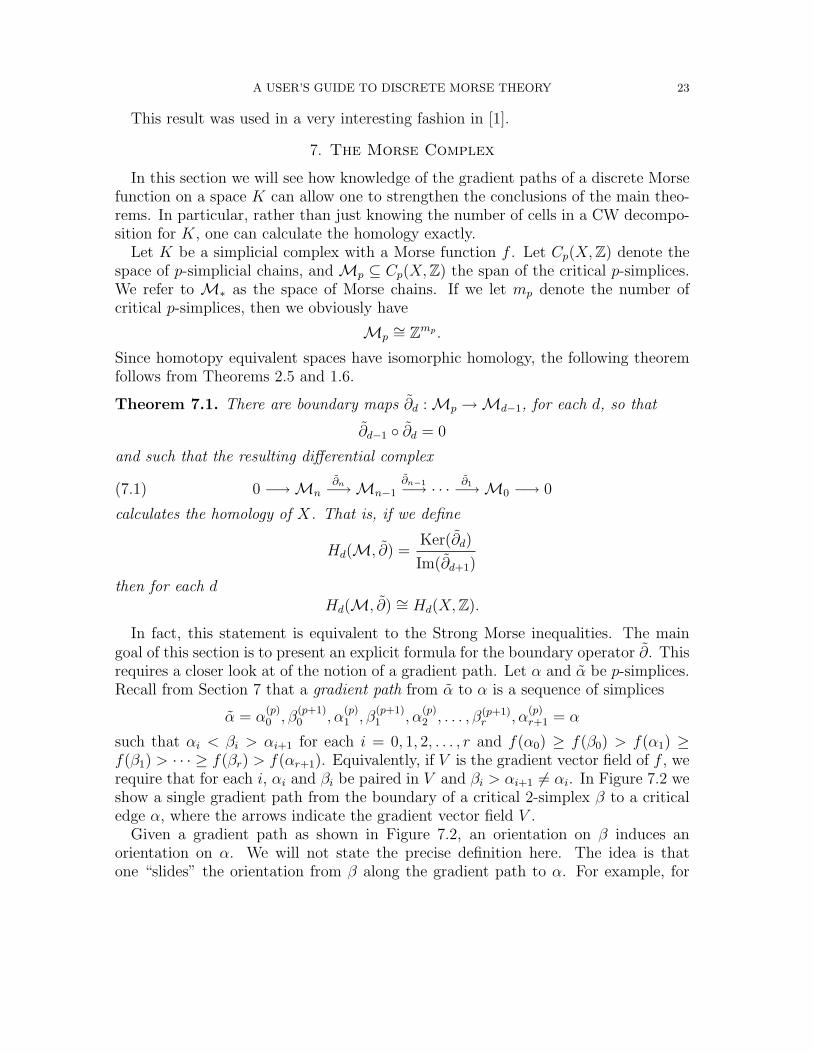
such that αi < βi > αi+1 for each i = 0, 1, 2, . . . , r and f(α0) ≥ f(β0) > f(α1) ≥f(β1) > · · · ≥ f(βr) > f(αr+1). Equivalently, if V is the gradient vector field of f , werequire that for each i, αi and βi be paired in V and βi > αi+1 6= αi. In Figure 7.2 weshow a single gradient path from the boundary of a critical 2-simplex β to a criticaledge α, where the arrows indicate the gradient vector field V .

Given a gradient path as shown in Figure 7.2, an orientation on β induces anorientation on α. We will not state the precise definition here. The idea is thatone “slides” the orientation from β along the gradient path to α. For example, for

24 ROBIN FORMAN

the gradient path shown in Figure 7.2, the indicated orientation on β induces theindicated orientation on α.

αβ

A gradient path from the boundary of β to α.

Figure 7.2.

We are now ready to state the desired formula.

Theorem 7.3. Choose an orientation for each simplex. Then for any critical (p+1)-simplex β set

(7.2) ∂β =∑

critical α(p)

cα,βα

wherecα,β =

∑γ∈Γ(β,α)

m(γ)

where Γ(β, α) is the set of gradient paths which go from a maximal face of β to α.The multiplicity m(γ) of any gradient path γ is equal to ±1, depending on whether,given γ, the orientation on β induces the chosen orientation on α, or the oppositeorientation. With this differential, the complex (7.1) computes the homology of K.

A proof of this theorem appears in Section 8 of [10]. We refer to the complex (7.1)with the differential (7.2) as the Morse complex (it goes by many different namesin the literature). An extensive study of the Morse complex in the smooth categoryappears in [36].

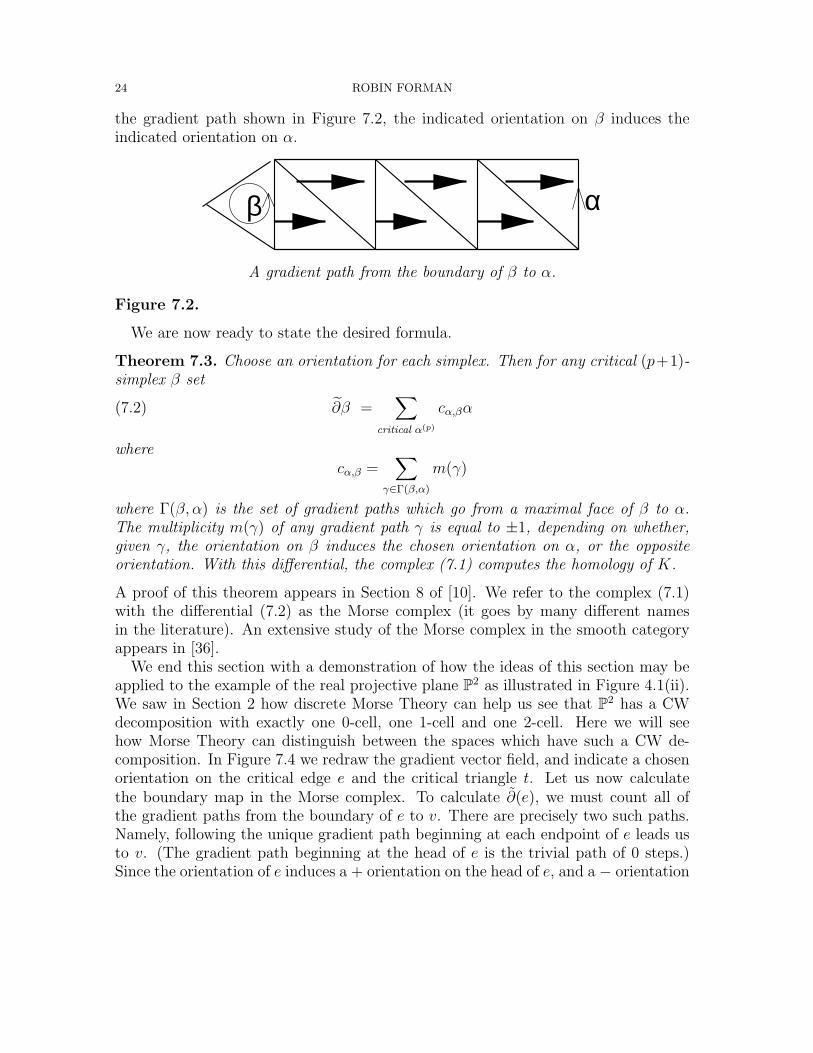
We end this section with a demonstration of how the ideas of this section may beapplied to the example of the real projective plane P2 as illustrated in Figure 4.1(ii).We saw in Section 2 how discrete Morse Theory can help us see that P2 has a CWdecomposition with exactly one 0-cell, one 1-cell and one 2-cell. Here we will seehow Morse Theory can distinguish between the spaces which have such a CW de-composition. In Figure 7.4 we redraw the gradient vector field, and indicate a chosenorientation on the critical edge e and the critical triangle t. Let us now calculatethe boundary map in the Morse complex. To calculate ∂(e), we must count all ofthe gradient paths from the boundary of e to v. There are precisely two such paths.Namely, following the unique gradient path beginning at each endpoint of e leads usto v. (The gradient path beginning at the head of e is the trivial path of 0 steps.)Since the orientation of e induces a + orientation on the head of e, and a − orientation


on the tail of e, adding these two paths with their corresponding signs leads us to theformula that ∂(e) = 0. It can be seen from the illustration that there are precisely twogradient paths from the boundary of t to e, and, with the illustrated orientation for t,both induce the chosen orientation on e, so that ∂(t) = 2e. Therefore the homologyof the real projective plane can be calculated from the following differential complex.

Z ×2−→ Z 0−→ Z −→ 0.

Thus we see that

H0(P2, Z) ∼= Z, H1(P2, Z) ∼= Z/2Z, H2(P2, Z) ∼= 0.

2

3

1

1 23

t

e

e

A gradient vector field on the real projective plane.

Figure 7.4.

8. Sphere Theorems

As mentioned in our discussion at the end of Section 4, one can sometimes usediscrete Morse Theory to make statements about more than just the homotopy typeof the simplicial complex. One can sometimes classify the complex up to homeomor-phism or combinatorial equivalence. This will be a very short section, as this topicseems a bit far from the main thrust of this paper. In addition, some terms will un-fortunately have to be defined only cursorily or not at all. So far, we have not placedany restrictions on the simplicial complexes under consideration. The main idea ofthis section is that if our simplicial complex has some additional structure, then onemay be able to strengthen the conclusion. This idea rests on some very deep work ofJ.H.C. Whitehead [44].

Recall that a simplicial complex K is a combinatorial d-ball if K and the standardd-simplex Σd have isomorphic subdivisions. A simplicial complex K is a combinato-rial (d− 1)-sphere, if K and Σd have isomorphic subdivisions (where Σd denotes theboundary of Σd with its induced simplicial structure). A simplicial complex K is a

26 ROBIN FORMAN

combinatorial d-manifold with boundary if the link of every vertex is either a combi-natorial (d− 1)-sphere or a combinatorial (d− 1)-ball. The following is a special caseof the main theorem of [44].

Theorem 8.1. Let K be a combinatorial d-manifold with boundary which simpliciallycollapses to a vertex. Then K is a combinatorial d-ball.

It is with this theorem (and its generalizations) that one can strengthen the con-clusion of Theorem 2.5 beyond homotopy equivalence. We present just one example.

Theorem 8.2. Let X be a combinatorial d-manifold with a discrete Morse functionwith exactly two critical simplices. Then X is a combinatorial d-sphere.

The proof is quite simple (given Theorem 8.1). If X is a combinatorial d-manifoldwith a discrete Morse function f with exactly two critical simplices, then the criti-cal simplices must be the minimum of f , which must occur at a vertex v, and themaximum of f , which must occur at a d-simplex α. Then X − α is a combinatoriald-manifold with boundary with a discrete Morse function with only a single criticalsimplex, namely the vertex v. It follows from Lemma 2.6 that X − α collapses to v.Whitehead’s theorem now implies that X−α is a combinatorial d-ball, which impliesthat X is a combinatorial d-sphere.

9. Cancelling Critical Points

One of the main problems in Morse Theory, whether in the combinatorial or smoothsetting, is to find a Morse function for a given space with the fewest possible criticalpoints (much of the book [38] is devoted to this topic). In general this is a verydifficult problem, since, in particular, it contains the Poincare conjecture — spherescan be recognized as those spaces which have a Morse function with precisely 2 criticalpoints. In [31], Milnor presents Smale’s proof [40] of the higher dimensional Poincareconjecture (in fact, a proof is presented of the more general h-cobordism theorem)completely in the language of Morse Theory. Drastically oversimplifying matters,the proof of the higher Poincare conjecture can be described as follows. Let M be asmooth manifold of dimension ≥ 5 which is homotopy equivalent to a sphere. EndowM with a (smooth) Morse function f . One then proceeds to show that the criticalpoints of f can be cancelled out in pairs until one is left with a Morse function withexactly two critical points, which implies that M is a (topological) sphere.

A key step in this proof is the “cancellation theorem” which provides a sufficientcondition for two critical points to be cancelled (see Theorem 5.4 in [31], which Milnorcalls “The First Cancellation Theorem”, or the original proof in [33]). In this sectionwe will see that the analogous theorem holds for discrete Morse functions. Moreover,in the combinatorial setting the proof is much simpler. The main result is that if α(p)

and β(p+1) are 2 critical simplices, and if there is exactly 1 gradient path from theboundary of β to α, then α and β can be cancelled. More precisely,


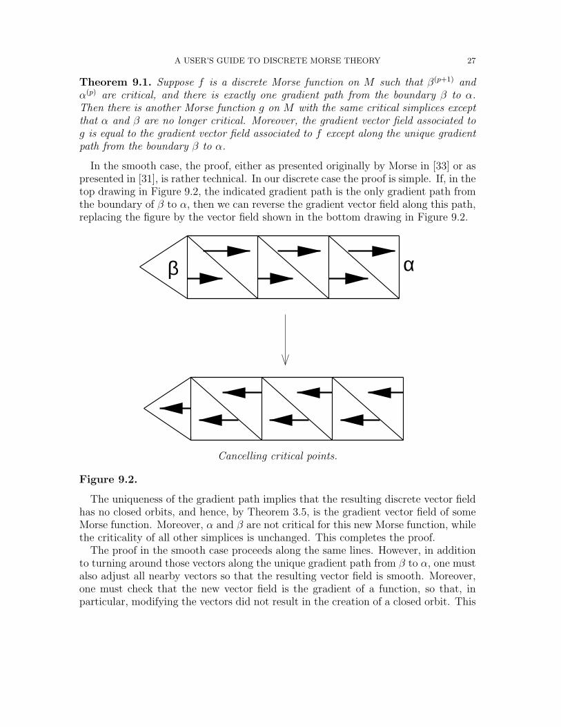
Theorem 9.1. Suppose f is a discrete Morse function on M such that β(p+1) andα(p) are critical, and there is exactly one gradient path from the boundary β to α.Then there is another Morse function g on M with the same critical simplices exceptthat α and β are no longer critical. Moreover, the gradient vector field associated tog is equal to the gradient vector field associated to f except along the unique gradientpath from the boundary β to α.

In the smooth case, the proof, either as presented originally by Morse in [33] or aspresented in [31], is rather technical. In our discrete case the proof is simple. If, in thetop drawing in Figure 9.2, the indicated gradient path is the only gradient path fromthe boundary of β to α, then we can reverse the gradient vector field along this path,replacing the figure by the vector field shown in the bottom drawing in Figure 9.2.

β α

Cancelling critical points.

Figure 9.2.

The uniqueness of the gradient path implies that the resulting discrete vector fieldhas no closed orbits, and hence, by Theorem 3.5, is the gradient vector field of someMorse function. Moreover, α and β are not critical for this new Morse function, whilethe criticality of all other simplices is unchanged. This completes the proof.

The proof in the smooth case proceeds along the same lines. However, in additionto turning around those vectors along the unique gradient path from β to α, one mustalso adjust all nearby vectors so that the resulting vector field is smooth. Moreover,one must check that the new vector field is the gradient of a function, so that, inparticular, modifying the vectors did not result in the creation of a closed orbit. This

28 ROBIN FORMAN

is an example of the sort of complications which arise in the smooth setting, butwhich do not make an appearance in the discrete theory.

This theorem was recently put to very good use in [2], in which discrete MorseTheory is used to determine the homotopy type of some simplicial complexes arisingin the study of partitions. It is fascinating, and quite pleasing, to see the same ideaplay a central role in two subjects, the Poincare conjecture and the study of partitions,which seem to have so little to do with one another.

10. Morse Theory and Evasiveness

So far, we have indicated some applications of discrete Morse Theory to combina-torics and topology. We now present an application to computer science. The readershould see the reference [14] for a more complete treatment of the content of thissection.

The problem we study is a topological version of a standard type of “search prob-lem”. The generalized version that we will present first appeared in [35]. Let S be ann-dimensional simplex, with vertices v0, v1, . . . , vn, and K a subcomplex of S whichis known to you. Let σ be a face of S which is not known to you. Your goal is todetermine if σ is in K. In particular, you need not determine the face σ, just whetheror not it is in K. You are permitted to ask questions of the form “Is vi in σ?”. Youmay use the answers to the questions you have already asked in determining whichvertex to ask about next. Of course, you can determine if σ is in K by asking n + 1questions, since by asking about all n + 1 vertices you can completely determine σ.You win this game if you answer the given question after asking fewer than n + 1questions.

Say that K is nonevasive if there is a winning strategy for this game, i.e thereis a question algorithm that determines whether or not σ ∈ K in fewer than n + 1questions, no matter what σ is. Say K is evasive otherwise.

Kahn, Saks and Sturtevant proved the following relationship between the evasive-ness of K and its algebraic topology.

Theorem 10.1. If H∗(K) 6= 0, where H∗(K) denotes the reduced homology of K,then K is evasive.

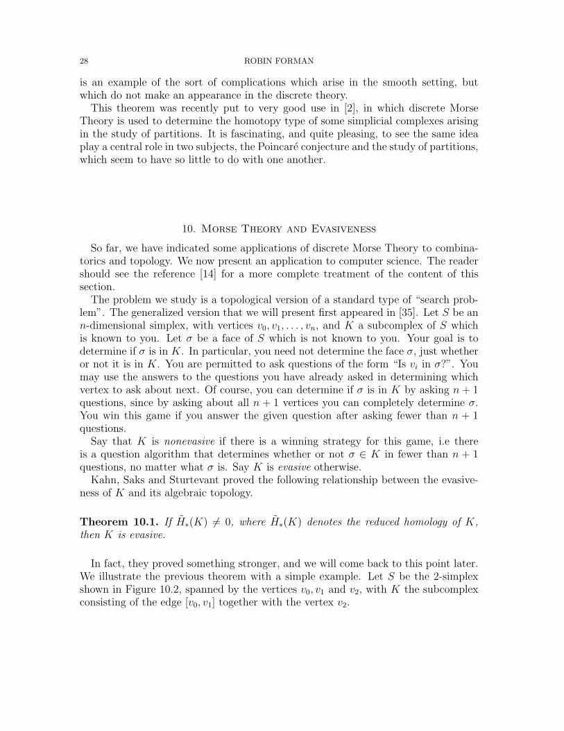
In fact, they proved something stronger, and we will come back to this point later.We illustrate the previous theorem with a simple example. Let S be the 2-simplexshown in Figure 10.2, spanned by the vertices v0, v1 and v2, with K the subcomplexconsisting of the edge [v0, v1] together with the vertex v2.


0

2

1v v

v

An example of an evasive subcomplex of the 2-dimensional simplex.

Figure 10.2.

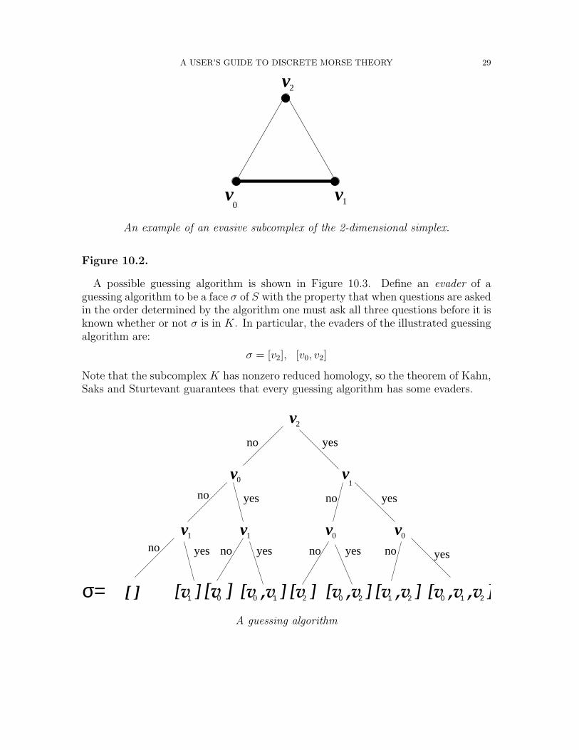
A possible guessing algorithm is shown in Figure 10.3. Define an evader of aguessing algorithm to be a face σ of S with the property that when questions are askedin the order determined by the algorithm one must ask all three questions before it isknown whether or not σ is in K. In particular, the evaders of the illustrated guessingalgorithm are:

σ = [v2], [v0, v2]

Note that the subcomplex K has nonzero reduced homology, so the theorem of Kahn,Saks and Sturtevant guarantees that every guessing algorithm has some evaders.

yes

v vv v

no

no noyes yes

v

v v

11 0 2 1 20[v ]σ= 2[v ]

yes noyes noyesno

1[v ] [v ,v ] [v ,v ] [v ,v ] [v ,v ,v ][ ]

no yes

0 2

2

1

0

0

0

1 01

A guessing algorithm

30 ROBIN FORMAN

Figure 10.3.

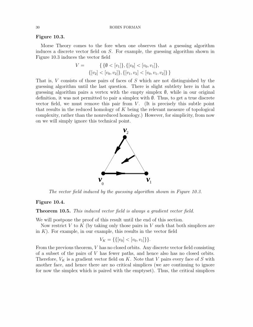
Morse Theory comes to the fore when one observes that a guessing algorithminduces a discrete vector field on S. For example, the guessing algorithm shown inFigure 10.3 induces the vector field

V = { {∅ < [v1]}, {[v0] < [v0, v1]},{[v2] < [v0, v2]}, {[v1, v2] < [v0, v1, v2]} }

That is, V consists of those pairs of faces of S which are not distinguished by theguessing algorithm until the last question. There is slight subtlety here in that aguessing algorithm pairs a vertex with the empty simplex ∅, while in our originaldefinition, it was not permitted to pair a simplex with ∅. Thus, to get a true discretevector field, we must remove this pair from V . (It is precisely this subtle pointthat results in the reduced homology of K being the relevant measure of topologicalcomplexity, rather than the nonreduced homology.) However, for simplicity, from nowon we will simply ignore this technical point.

0

2

1v

v

vThe vector field induced by the guessing algorithm shown in Figure 10.3.

Figure 10.4.

Theorem 10.5. This induced vector field is always a gradient vector field.

We will postpone the proof of this result until the end of this section.Now restrict V to K (by taking only those pairs in V such that both simplices are

in K). For example, in our example, this results in the vector field

VK = {{[v0] < [v0, v1]}}.From the previous theorem, V has no closed orbits. Any discrete vector field consistingof a subset of the pairs of V has fewer paths, and hence also has no closed orbits.Therefore, VK is a gradient vector field on K. Note that V pairs every face of S withanother face, and hence there are no critical simplices (we are continuing to ignorefor now the simplex which is paired with the emptyset). Thus, the critical simplices


of VK are precisely the simplices of K which are paired in V with a face of S which isnot in K. These are precisely the simplices of K which are the evaders of the guessingalgorithm.

The Morse inequalities of Theorem 2.11 (i) imply that the number of evaders in K

is at least dim H∗(K). Evaders occur in pairs, with each pair having one face of K andone face not in K. This yields the following quantitative refinement of Theorem 10.1.

Theorem 10.6. For any guessing algorithm

# of evaders ≥ 2 dim H∗(K)

Suppose that K is nonevasive. Then there is some guessing algorithm which hasno evaders. From our above discussion we have seen that this implies that K has agradient vector field with no critical simplices. Actually, this is not quite true. Thegradient vector field must have a critical vertex — the vertex that is paired with theempty set — this is that minor technicality that we have been ignoring. ApplyingLemma 2.6 yields the following strengthening of Theorem 10.1.

Theorem 10.7. If K is nonevasive, then K simplicially collapses to a point.

This theorem appears in [23]. The interested reader can consult [14] for some addi-tional refinements of this theorem.

We end this section with a proof of Theorem 10.5. Fix a subcomplex K of an n-simplex S, and a guessing algorithm. Associate to each p-simplex α of S the sequenceof integers

n(α) = n0(α) < n1(α) < · · · < np(α)

where the ni(α)’s are the numbers of the questions answered “yes” if σ = α.If V is the vector field induced by the guessing algorithm and

α(p)0 , β

(p+1)0 , α

(p)1

is a V -path, then {α0, β0} is in V , which means that α0 and β0 are not distinguisheduntil the (n + 1)st question. Thus,

n(β0) = n0(α0) < n1(α0) < · · · < np(α0) < n + 1.

We now observe that the vertices of a1 are a subset of the vertices of b0. Suppose thevertex of β0 which is not in α1 is the vertex tested in question ni(β0). Then we musthave i 6= n + 1 (since α0 6= α1). This demonstrates that

n(α1) = n0(α0) < n1(α0) < · · · < ni−1(α0) < ni(α1) < . . .

for some i < n + 1, and such that ni(α1) > ni(α0). Thus n(α1) > n(α0) in thelexicographic order, which is sufficient to prove that there are no closed orbits.

QED

32 ROBIN FORMAN

11. Further Thoughts

We close this paper with some additional thoughts on the subjects discussed in thispaper.

I would like to begin by encouraging the reader to take a look at the papers [24],[25], and [3]. In these papers, discrete Morse Theory is used to investigate quiteinteresting problems. These references were not mentioned earlier only because theydid not easily fit into any of the previous sections of this paper.

There are a number of directions in which discrete Morse Theory can be extendedand generalized. Here we mention a few such possibilities. In [16] we show how onecan recover the ring structure of the cohomology of a simplicial complex from thepoint of view of discrete Morse Theory (this follows work of Betz and Cohen [4] andFukaya [17, 18] in the smooth setting). In [34], Novikov presents a generalizationof standard smooth Morse Theory in which the role of the Morse function is nowplayed by a closed 1-form (the classical case arises when the closed 1-form is exact).In [15] we present the analogous generalization for discrete Morse Theory. In [45],Witten shows how smooth Morse Theory can be seen as arising from considerationsof supersymmetry in quantum physics. In [11] we present a combinatorial version ofWitten’s derivation. We believe that this latter work may have greater significance.At crucial points in [45], Witten appeals to path integral arguments which are ratherstandard in quantum physics, but are ill-defined mathematically. In the correspondingmoments in [11] what arises is a well-defined discrete sum. Perhaps the approach in[11] can find uses in the analysis of other quantum field theories.

One topic which we have only touched upon is the study of the dynamics associatedto flowing along the gradient vector field associated to a discrete Morse function. Infact, an understanding of the dynamics is crucial to the proof of theorem 7.3, forexample. The relevant study takes place in Section 6 of [10]. In [12] we study thedynamical properties of the flow associated to a general discrete vector field.

One area in which much work remains to be done is the investigation of discreteMorse Theory for infinite simplicial complexes. The theory as described in this papercan be applied without change to an infinite simplicial complex K endowed with adiscrete Morse function f which is proper, i.e., one in which for each real number cthe level subcomplex K(c) is a finite complex. Unfortunately, properness is often anunnatural requirement when considering the infinite simplicial complexes which arisein practice. In the interesting paper [29], discrete Morse Theory is applied to theinvestigation of infinite simplicial complexes K which arise as a covering space of afinite simplicial complex K ′. In this case, the authors restrict attention to discreteMorse functions which are lifts of a Morse function on K ′, and compare the numberof critical simplices to the L2-Betti numbers of K. While it appears to be too muchto hope that one can develop a useful theory that applies to all infinite simplicialcomplexes with no restrictions on the discrete Morse function, it seems likely that


there is room for very useful investigations of large classes of complexes and functionswith restrictions different than those already considered.

I will close these notes with some comments of a less rigorous nature. Whether inthe smooth category or the combinatorial category, Morse Theory is not essential toany problem, it is usually “only” a convenient and efficient language. Anything thatcan be done with Morse Theory can be done without it. It seems to me that MorseTheory takes on a special significance in three different cases. First are the cases inwhich Morse Theory is not intrinsic to the problem, but where the existence of suchan efficient language may make the difference between whether or not one is able tosee the way to the end of a problem. The best example of this in the smooth setting, Ithink, is the proof of the higher dimensional Poincare conjecture ([39], [31]). Most ofthe applications of discrete Morse Theory mentioned in Section 5, for example, seemto fall into this category. Second are the cases in which the space one is studyingcomes naturally endowed with a Morse function, or a gradient vector field. Here theprime example is Bott’s proof of Bott periodicity ([5], see also Part IV of [30]), restingon the fact that the loop space of a Riemannian manifold is endowed with a naturalMorse function. In the combinatorial setting, I would place the Morse-theoretic ex-amination of evasiveness of the previous section in this category. Third are the casesin which the objects under investigation can be naturally identified as the criticalpoints of a Morse function on a larger space. Examples of this phenomenon aboundin differential geometry, where one often studies extremals of energy functionals. Inparticular, Morse’s first great triumph with Morse Theory was his investigation of theset of geodesics between two points in a Riemannian manifold ([32], see also Part IIIof [30]). The geodesics are precisely the critical points of the natural Morse functionon the path space, and Morse used the Morse inequalities, along with a knowledgeof the topology of the path space, to deduce the existence of many critical points.It is intriguing to this author that there are as yet no corresponding examples inthe combinatorial setting. I know of no examples in which a collection of classicallystudied objects in combinatorics can be naturally identified with the critical simplicesof a Morse function on some larger complex. Indeed, I believe that soon combinato-rial examples of interest will be found that fit into this third category. I wonder ifapplications of discrete Morse theory will be found that approach the beauty, depthand fundamental significance of the applications of smooth Morse Theory mentionedin this paragraph.

On a broader note, I believe that discrete Morse Theory is only a small part of whatsomeday will be a more complete theory of “combinatorial differential topology”,although I hesitate to predict (at least in print) what form such a theory will take.

34 ROBIN FORMAN

References

[1] E. Babson, A. Bjorner, S. Linusson, J. Shareshian and V. Welker, Complexes of not i-Connected Graphs, Topology 38 (1999), pp. 271-299.

[2] E. Babson, P. Hersh, Discrete Morse functions from lexicographic orders, to appear inTopology.

[3] E. Batzies and V. Welker Discrete Morse Theory for Cellular Resolutions, J. Reine Angew.Math. 543 (2002), pp. 147–168.

[4] M. Betz and R. Cohen, Graph moduli space and cohomology operations, Turk. J. of Math.18 (1994), pp. 23-41.

[5] R. Bott, Stable homotopy of the classical groups, Ann. of Math. 70 (1959), pp. 313-337.[6] M. Chari, On Discrete Morse Functions and Combinatorial Decompositions, Discrete

Math. 217 (2000), pp. 101-113.[7] X. Dong, The Topology of Bounded Degree Graph Complexes and Finite Free Resolutions,

thesis, Univ. of Minn., 2001.[8] A. Duval A Combinatorial Decomposition of Simplicial Complexes, Israel J. of Math. 87

(1994), pp. 77-87.[9] R. Forman, A Discrete Morse Theory for Cell Complexes, in: Geometry, Topology &

Physics for Raoul Bott, S.T. Yau (ed.), International Press, 1995.[10] , Morse Theory for Cell Complexes, Adv. in Math. 134 (1998), pp. 90-145.[11] , Witten-Morse Theory for Cell Complexes, Topology 37 (1998), pp. 945-979.[12] , Combinatorial Vector Fields and Dynamical Systems, Math. Zeit. 228 (1998),

pp. 629-681.[13] , Combinatorial differential topology and geometry, in: New Perspectives in Alge-

braic Combinatorics (Berkeley, CA. 1996-97), Math. Sci. Res. Inst. Publ. 38, CambridgeUniv. Press, Cambridge, 91999), pp. 177-206.

[14] , Morse Theory and Evasiveness, Combinatorica 20 (2000), pp. 498-504.[15] , Novikov-Morse theory for cell complexes, to appear in Int. J. of Math.[16] The Cohomology Ring and Discrete Morse Theory, preprint 2001.[17] K. Fukaya, Morse homotopy, A∞-category, and Floer homologies, in: Proc. Garc. Work-

shop on Geometry and Topology ’93, (Seoul, 1993), ed. H. J. Kim, Lecture Notes Ser. 18,Seoul National University, pp 1-102.

[18] , Morse homotopy and its quantization, in: Geometric Topology (Athens, GA1993),AMS/IP Stud. Adv. Math21, Amer. Math. Soc., Prov. RI, 1997, pp. 409-440.

[19] M. Goresky and R. MacPherson Stratified Morse Theory, in: Singularities, Part I (Arcata,CA, 1981), Proc. Sympos. Pure Math., 40, Amer. Math. Soc., R.I., (1983), pp. 517-533.

[20] Stratified Morse Theory, Ergebnisse der Mathematik und ihrer Grenzgebiete (3),14, Springer Verlag, Berlin-New York, 1988.

[21] J. Jonsson, On the homology of some complexes of graphs, preprint, 1998.[22] , The decision tree method, preprint, 1999.[23] J. Kahn, M. Saks and D. Sturtevant A topological approach to evasiveness, Combinatorica

4 (1984), pp. 297-306.[24] D. Kozlov, Collapsibility of ∆(Πn)/Sn and some related CW complexes, Proc. Amer.

Math. Soc. 128 (2000), pp. 2253-2259.[25] , Topology of spaces of hyperbolic polynomials with multiple roots, to appear in

Israel J. Math.[26] W. Kuhnel, Triangulations of Manifolds with few Vertices, in: Advances in Differential

Geometry and Topology, World Sci. Publishing, N.J., (1990), pp. 59-114.


[27] S. Linusson and J. Shareshian, Complexes of t-colorable graphs, preprint.[28] A. Lundell and S. Weingram, The Topology of CW Complexes, Van Nostrand Reinhold

Company, New York, 1969.[29] V. Mathai and S.G. Yates, Discrete Morse theory and extended L2 homology, J. Funct.

Anal. 168 (1999), pp. 84–110.[30] J. Milnor Morse Theory, Annals of Mathematics Study No. 51, Princeton University Press,

1962.[31] , Lectures on the h-Cobordism Theorem Princeton Mathematical Notes, Princeton

University Press, 1965.[32] M. Morse, The Calculus of Variations in the Large, Amer. Math. Soc. Colloquium Pub.

18, Amer. Math. Soc., Providence R.I., (1934).[33] , Bowls of a Non-Degenerate Function on a Compact Differentiable Manifold, in:

Differential and Combinatorial Topology (A Symposium in Honor of M. Morse), PrincetonUniversity Press (1965), pp. 81-104.

[34] S. Novikov, Multivalued functions and functions: An analogue of the Morse theory, SovietMath. Dokl. 24 (1981), pp. 222-226.

[35] R.L. Rivest and J. Vuillemin On recognizing graph properties from adjacency matrices,Theor. Comp. Sci. 3 (1976), pp. 371-384.

[36] M. Schwartz, Morse Homology Progress in Mathematics, 111, Birkhauser Verlag, Basel(1993).

[37] J. Shareshian, Discrete Morse Theory for Complexes of 2-Connected Graphs, to appearin Topology.

[38] V. Sharko, Functions on Manifolds, Algebraic and Topological Aspects, Trans. of Math.Monographs 131, Amer. Math. Soc., Providence, R.I., (1993).

[39] S. Smale, On Gradient Dynamical Systems, Annals of Math. 74 (1961), pp. 199-206.[40] The Generalized Poincare Conjecture in Dimensions Greater than Four, Annals of

Math. 74 (1961), pp. 391-406.[41] R. Stanley, A Combinatorial Decomposition of Acyclic Simplicial Complexes, Discrete

Math. 120 (1993), pp. 175–182.[42] V. Turchin, Homology of Complexes of Biconnected Graphs, Uspekhi Mat. Nauk. 52

(1997), pp. 189-190; translation in Russian Math. Surveys 52 (1997), 426–427.[43] V. Vassiliev, Complexes of Connected Graphs, in: The Gelfand Mathematical Seminars,

1990–1992, pp. 223–235. Birkhauser Boston, Boston, (1993).[44] J.H.C. Whitehead, Simplicial Spaces, Nuclei, and m-Groups, Proc. London Math. Soc.

45 (1939), pp. 243-327.[45] E. Witten Supersymmetry and Morse Theory J. Diff. Geom. 17 (1982), pp. 661–692.

Department of Mathematics, Rice University, Houston, TX 77251

Documents

S´eminaire Lotharingien de Combinatoire 48 (2002), Article B48c