SELF-TARGETING:EVIDENCE FROM A FIELD EXPERIMENT IN INDONESIA

VIVI ALATAS, ABHIJIT BANERJEE, REMA HANNA,BENJAMIN A. OLKEN, RIRIN PURNAMASARI, AND MATTHEW WAI-POI

Abstract. In this paper, we show that adding a small application cost to a social assistanceprogram can substantially improve targeting because of the self-selection it induces. We conducta randomized experiment within Indonesia’s Conditional Cash Transfer program that comparestwo of the most common methods of targeting welfare programs in the developing world: in one,beneficiaries first need to apply for the program, and then an enumerator visits them at homeand determines their eligibilty based on a proxy-means asset test; in the other, they are visiteddirectly by the enumerator and automatically enrolled if they qualify based on the same proxy-means test. When applications were required, we find that the poor are more likely to apply thanthe rich, even conditional on whether they would pass the asset test. On net, the villages whereapplications were required have a much poorer group of beneficiaries than automatic enrollmentvillages. However, marginally increasing the cost of applying does not necessarily improve targeting:while experimentally increasing the distance to the application site reduces the number of applicants,it screens out both rich and poor in roughly equal proportions. Estimating our model of theenrollment choice suggests that our results are largely driven by the rich forecasting that they havea very small likelihood of passing the asset test, and so not bothering to apply, which in aggregatesubstantially improves targeting efficiency. The results suggest that the combination of the smallcost and the final screening gives this class of mechanisms the ability to achieve many of the benefitsof self-selection without imposing onerous ordeals on program beneficiaries.

Date: November 2013.Affiliations: Alatas, Purnamasari, Wai-Poi: World Bank. Banerjee, Olken: MIT, BREAD, CEPR, J-PAL, andNBER. Hanna: Harvard Kennedy School, BREAD, CEPR, J-PAL, and NBER. Contact email: bolken@mit.edu.This project was a collaboration involving many people. We thank Jie Bai, Talitha Chairunissa, Amri Ilmma,Donghee Jo, Chaeruddin Kodir, He Yang, Ariel Zucker, and Gabriel Zucker for their excellent research assistance,and Raj Chetty, Esther Duflo, Amy Finkelstein, and numerous seminar participants for helpful comments. We thankMitra Samya, the Indonesian Central Bureau of Statistics (BPS), the Indonesian National Team for the Accelerationof Poverty Reduction (TNP2K, particularly Sudarno Sumarto and Bambang Widianto), the Indonesian Social AffairsDepartment (DepSos), and SurveyMetre for their cooperation implementing the project. Most of all, we thank JuristTan for her truly exceptional work leading the field implementation. This project was financially supported by theWorld Bank, AusAID, and 3ie, and analysis was supported by NIH under grant P01 HD061315. All views expressedare those of the authors and do not necessarily reflect the views of the World Bank, TNP2K, Mitra Samya, DepSos,or the Indonesian Central Bureau of Statistics.

1

1. Introduction

In designing targeted aid programs, a perennial problem is how to separate the poor from therich. One strategy for doing so is to impose program requirements that are differentially costly forthe rich and the poor, in order to induce the poor to participate while dissuading the rich fromdoing so (Nichols, Smolensky and Tideman, 1971; Nichols and Zeckhauser, 1982; Ravallion, 1991;Besley and Coate, 1992). These “ordeal” mechanisms are quite common: welfare programs, fromthe Works Progress Administration (WPA) in the United States during the Great Depression tothe National Rural Employment Guarantee Act (NREGA) right-to-work scheme in India today,often have manual labor requirements to receive aid, and subsidized food schemes often providelower quality food so that those who can afford tastier food choose not to purchase the subsidizedproducts.

The challenge with these ordeal mechanisms is that they can be quite inefficient: in order todissuade the rich from participating, the poor are forced to incur substantial utility costs in orderto receive transfers, whether by toiling in the hot sun or eating unappetizing food. In this paper, weask whether much smaller costs can still achieve substantial self-selection. In particular, we showthat when the cost entails applying for benefits, and there is some ex-ante uncertainty in whetheran application will be successful, even small application costs can generate significant improvementsin targeting. The reason is that if the rich correctly foresee that they face only a very small chanceof slipping through the screening procedure and receiving benefits, they may not bother to apply,and the resulting reductions in inclusion error may substantially improve the degree to which theprogram is targeted to the poor. Self-selection can also reduce the degree to which the poor areexcluded from the program compared to alternative, top-down targeting schemes if it encouragesthe very poor who live at the margins of society to make themselves known to government staff byapplying for the program.

Of course, it is not ex-ante obvious that these types of application costs will necessarily improvetargeting. The recent movement in behavioral economics, for example, has emphasized that peopletend to over-respond to small costs, and that these types of application costs may dissuade the poorfrom applying. For example, the hassle costs with applying for social assistance programs, such asfood stamps and welfare payments, have been cited as a reason for low takeup of these programs, andthere have been policy suggestions that these types of hassles should be removed from applicationprocesses to encourage program takeup (Bertrand, Mullainathan and Shafir, 2004; Currie, 2006). Itis also theoretically possible that the poor face a variety of other deterrents from applying, such asself-control problems (e.g., Madrian and Shea, 2001), stigma (e.g., Moffitt, 1983), and poor accessto information about government programs (e.g., Daponte, Sanders and Taylor, 1999). Ultimately,whether making people apply for programs achieves better targeting than automatic enrollment isan empirical question.

In this paper, we investigate whether in fact making people apply for programs improves orworsens targeting by conducting a randomized experiment in the context of Indonesia’s ConditionalCash Transfer program, known as PKH. Conditional cash transfer programs have spread rapidlythroughout the developing world and are present in over 30 countries today. In Indonesia, thePKH program provides beneficiaries with US $130 per year for 6 years, and is one of the country’s

2

largest social assistance programs, aiding about 2.4 million households. The program is aimed atthe poorest 5-10 percent of the population, with eligibility determined based on a weighted sumof about 30 easy-to-observe assets (e.g., size of house, materials used to construct household roof,motorbike ownership).

Working with the Indonesian government, we experimentally varied the enrollment process forPKH across 400 villages, comparing a process that required potential applicants to apply for theprogram to the status quo, where eligible households were surveyed by the government and wereautomatically enrolled if they qualified. In both cases, eligibility was determined based on anasset screen, known as a proxy-means test (PMT), so the key difference we studied was whetherhouseholds had to actively apply or were instead automatically enrolled based on a governmentsurvey. These two approaches to targeted social-assistance programs – automatic enrollment basedon a top-down survey or enrollment being limited to who actively apply – represent the two mostcommon ways of determining beneficiary lists for targeted transfer programs in the developing world(Grosh et al., 2008; Kidd and Wylde, 2011).1

In our study, in villages randomized to receive the application process (henceforth “self-targeting”villages), households that were interested in the program were required to go to a central registrationsite to take an asset test administered by the statistics office. This entailed both traveling a fewkilometers to the application site and waiting in line to apply. Within these areas, we randomlyvaried the application costs along two dimensions: the distance to the application site and whetherone or both spouses needed to be present to apply. These application costs – missing about a halfday’s work, and traveling a few kilometers – pale in comparison to the benefits on offer, whichamount to $130 per year for 6 years. In control areas, the status quo procedure – automaticenrollment – was followed: the statistics office, working with local government officials, drew up alist of potential beneficiaries; interviewed everyone at their homes; and then automatically enrolledthose who passed using the same asset test that was used in self-targeting.

We begin with a description of the experiment and the data. We then ask what we would expectfrom such an experiment on purely a priori grounds. Specifically, we adapt the classical theory ofself-selection into social programs developed by Nichols, Smolensky and Tideman (1971), Nicholsand Zeckhauser (1982), Besley and Coate (1992) and others to a context where after selecting intoapplying, one receives the program stochastically, with the probability of receiving the programdeclining with income. The fact that receiving benefits is stochastic but declining with incomecaptures the fact that most screening mechanisms, including but not limited to proxy-means tests,do differentiate between rich and poor, but not perfectly, so that people cannot exactly forecastbefore applying whether they will in fact be eligible.2 The standard Nichols and Zeckhauser (1982)

1Examples of automatic enrollment PMTs include the Mexican Progresa program, the Columbian social assistanceprograms, and the Indonesian cash transfer programs; examples of self-selection based PMTs include the expansionof Progresa under the name Oportunidades to urban areas, the Chilean social assistance system, the Costa RicanSIPO system, and the Mongolian Child Money Program (Castaneda and Lindert, 2005; Hodges et al., 2007; Coadyand Parker, 2009; Martinelli and Parker, 2009).2The fact that people cannot perfectly forecast program eligibility before applying is not just limited to developingcountry contexts; in the Oregon Health Insurance Experiment, for example, about half of those who applied for thehealth insurance were in fact ineligible, a much lower rate than one would expect from the population at large butstill substantial (Finkelstein et al., 2012).

3

self-selection idea depends on a single-crossing property, where the ordeal is more costly for richthan poor. Time-based ordeals are the canonical example, since the rich presumably have a higheropportunity cost of time than the poor. In this context, we illustrate that there are a number ofreasons why requiring people to spend time traveling to the application site and applying need notnecessarily generate single-crossing: the poor and rich may have different tools for overcoming thecosts which may make them less costly for the rich; there may be income effects so that the samemonetary cost imposes a differential utility cost on the poor; and the distribution of idiosyncraticcosts of applying may mean that there are more poor on the margin of being deterred by increases incosts than rich. On the other hand, the fact that the probability of receiving benefits is downwardsloping in income is a strong force in favor of self-targeting improving targeting: since the richface only a very small chance of passing through the proxy-means test if they apply, they may notbother, even if the costs are relatively small.

Our empirical analysis then proceeds in four stages. First, we begin by examining who chooses toself-select into applying for the program in the 200 villages with the application-based process. Todo so, we utilize data on households’ per capita consumption that we collected before the programwas announced or targeting began. We find that the probability of self-selecting to apply for theprogram is decreasing in a household’s per capita consumption, i.e., that the poor are always morelikely to apply than the rich. Decomposing consumption into that which is potentially observable tothe government (i.e. the part that can be predicted based on observable assets) and the unobservableresidual, we show that those who apply are poorer on both observables and unobservables than thosewho choose not to apply. This implies that self-selection can not only potentially save resources(since many who would fail the asset test, i.e., have high observables, are no longer tested), but thatit also has the potential to improve targeting even over a universally-administered asset test (sincethose that apply are poorer on unobservables than the population at large). However, we also findevidence for the view that self-targeting may screen out some of the poor: for example, only about60 percent of the very poorest apply under self-targeting.

The question, though, for most governments is not necessarily how self-targeting would performrelative to a counterfactual of no error, but rather how it would compare against the next bestalternative targeting strategy. The second step of our empirical analysis is to use the experimentto compare self-targeting with the status quo of automatic-enrollment, in which the governmentconducted the asset test for all potential beneficiaries (chosen through prior asset surveys andconsultations with village leadership) at their homes and automatically enrolled those that passed.Compared against this real alternative, we find that per capita consumption was 21 percent lower forbeneficiaries in the self-targeting villages than those under the status quo. Moreover, exclusion errorwas actually less of a problem in self-targeting than in the status quo: the very poorest householdswere twice as likely to receive benefits in self-targeting than in control areas. These findings are notentirely driven by the fact that the government ineptly chose whom to interview under the statusquo: supplementing the government’s asset test data in the automatic enrollment villages withasset data that we independently collected for those not interviewed, we find that the beneficiariesunder self-targeting would still be, on average, poorer than those under a “hypothetical” universalautomatic enrollment system where everyone is interviewed for the asset test. Intuitively, this is

4

possible because – as we showed above – self-selection includes selection on unobservables. That is,conditional on passing the asset test, those that self-select into applying have lower consumptionthan the average person in the population.

The third step in our empirical analysis is to consider whether marginal increases in the severityof the ordeal further increase targeting performance. We examine the results from experimentallyvarying the distance to the registration site (increasing travel costs) and the number of householdmembers required to be present at the application site (increasing opportunity costs of time forthe family). We find no evidence that these marginal increases in application costs further improveselection. In some cases, they reduce overall takeup, but they do not differentially discriminatebetween rich and poor.

The theoretical model outlines a number of reasons why marginal increases in the extent of ordealsmight not necessarily improve targeting. To understand which factors are in fact empirically relevantfor takeup, the final step of our empirical analysis uses Generalized Method of Moments to estimatea CRRA utility version of our model with logit shocks. We use the average show-up rates in thefar distance treatment for each income quintile as moments. Since we estimate the model usingonly one experimental sub-treatment and cross-sectional differences in distances to fit the model,not the experimental variation, we can check that the model’s predictions provide a reasonableapproximation of the experimental findings, which indeed they do.

We use the estimated version of the model to see which of the various mechanisms we outlinedin the theoretical section lie behind the fact that marginal increases in the extent of the ordeal donot seem to differentially improve selection. Simulations from the estimated model suggest that,of the theoretical mechanisms we outline, neither curvature of the utility function nor differentialtravel technology is driving that result. Instead, the model suggests that the key driver of selectionis the fact that rich households forecast that they have a very small likelihood of receiving benefitsconditional on applying and therefore do not bother to apply if there is any cost of applying. Thishelps explain both why small costs can produce substantial selection but marginally increasing theintensity of the costs reduces overall application rates without substantially improving targeting.

The remainder of the paper is organized as follows. Section 2 discusses the setting, experimentaldesign, and data. Section 3 introduces our model,which revisits the standard screening model in lightof curvature in the utility function, differential access ways of dealing with costs, and idiosyncraticshocks. Section 4 examines the self-targeting data to ask who chooses to apply for the program.Section 5 uses the experiment to compare self-targeting with the status quo PMT-based approach.Section 6 examines the marginal effect of targeting when the ordeal is changed experimentally.Section 7 estimates the model to help shed light on which of the possible theoretical mechanismswe outline best explains the results. Section 8 concludes.

2. Setting and Experimental Design

2.1. Setting: The PKH Program. This project explores self-targeting mechanisms within thecontext of Program Keluarga Harapan (PKH), a conditional cash transfer project administeredby the Ministry of Social Affairs (DepSos) in Indonesia. The program targets households withper capita consumption below 80 percent of the poverty line (approximately the poorest 5 percent

5

of the population we study) and that meet the demographic requirements of having a pregnantwoman, a child between the ages of 0 to 5, or children below the age of 18 years old that havenot finished the nine years of compulsory education. Program beneficiaries receive direct cashassistance ranging from Rp. 600,000 to Rp. 2.2 million (US$67-US$250) per year—or about 3.5 to13 percent of the average yearly consumption by very poor households in our sample—depending ontheir family composition, school attendance, pre/postnatal check-ups, and completed vaccinations.3

The payments are disbursed quarterly for up to six years. In 2013, approximately 2.4 millionhouseholds are enrolled in the program. Determining whether households fall below the consumptionrequirement (“targeting”) is difficult because per capita consumption is not easily observed by thegovernment. Instead, PKH uses a proxy-means test (PMT) approach with automatic enrollment forall households that meet the demographic requirements and pass a proxy-means test. Specifically,every three years, enumerators from the Central Statistical Bureau (BPS) conduct a survey ofhouseholds nationwide who are potentially eligible for anti-poverty programs, including but notlimited to PKH. They survey all households that were included on previous surveys (regardlessof whether they previously qualified or not) and supplement this list with recommendations fromlocal leaders and their own observations of the kinds of houses that the households inhabit. Afterpassing an initial pre-screening, each household is asked a series of about 30 questions, includingattributes of their home (e.g., wall type, roof type), ownership of specific assets (e.g., motorcycle,refrigerator), household composition, and the education and occupation of the household head.These measures are combined with location-based indicators, such as population density, distanceto the district capital and access to education. Using independent survey data, the governmentthen estimates the relationship between these variables and the household per capita consumptionto generate a district-level formula for predicting consumption levels based on the responses to thesurvey. Individuals with predicted consumption levels below each district’s very poor line wereeligible for the program.

Figure 1 shows the probability of passing the asset test and being determined eligible for theprogram as a function of log per-capita income, as estimated from our baseline data. Note thatthe particular function used to map assets to eligibility is estimated by the government separatelyfor each district and for urban and rural areas, which is why several different downward-slopingcurves are visible in the Figure. Several key points are worth observing about this function. First,it is strongly downward sloping – the poor are much more likely to receive benefits than the rich.Second, there is substantial noise in the process, driven by how hard it is to accurately estimateconsumption from assets and the fact that PKH targets the bottom approximately 5 percent of thepopulation – even the very poorest rarely have more than a 40 percent chance of receiving benefits,and even those with incomes more than twice the target threshold (i.e. about 13 log points, asopposed to the cutoff of about 12.3 log points) still have as much as a 5 to 10 percent chance ofreceiveing benefits.4

3Note, however, that although PKH is formally a conditional cash transfer program, with transfers dependent uponhealth takeup and school enrollment, these conditions are typically not enforced in practice, so this can be thoughtof as closer to a ‘labeled’ cash grant, as in Benhassine et al. (2013).4The regressions of income on assets underlying Figure 1 have an R2 of between 0.4-0.6. One might be concernedthat the relatively poor prediction in Figure 1 is simply because the government is using the wrong algorithm. Thisdoes not, however, appear to be the case. In separate ongoing work, we have examined a wide range of non-linear

6

2.2. Sample Selection. This project was carried out during the 2011 expansion of PKH to newareas. We chose 6 districts (2 each in the provinces of Lampung, South Sumatra, and CentralJava) from the expansion areas to include a wide variety of cultural and economic environments.Within these districts, we randomly selected a total of 400 villages, stratified such that the finalsample consisted of approximately 30 percent urban and 70 percent rural locations.5 Within eachvillage, we randomly selected one hamlet to be surveyed.6 These hamlets are best thought of asneighborhoods that consist of about 150 households and that each has its own administrative head,whom we refer to as the hamlet head.

2.3. Experimental Design. We randomly allocated each of the 400 villages to one of two targetingmethodologies: self-targeting or an automatic enrollment system, i.e. the status quo.7

2.3.1. Automatic Enrollment Treatment. In Indonesia, the automatic enrollment treatment is thestatus quo, and the procedure discussed in Section 2.1 was followed. For each hamlet in thistreatment, the government Bureau of Statistics (BPS) enumerators were given a pre-printed listof households from the last targeting survey (PPLS, 2008). When they arrived at a village, theenumerators showed the list to the village leadership and asked them to add any households to thelist that they thought were inappropriately excluded. The enumerators also had the option of addinghouseholds to the list of interviewees if they observed that a household was likely to be quite poor.For each household that was interviewed, a computer-generated poverty score was generated usingthe district-specific PMT formulas.8 A list of beneficiaries was generated by selecting all householdswith a predicted score below the score cutoff for their district. 9

machine learning algorithms to see if they can improve the predictive power in Figure 1, which is based on OLS. Wefound only very small improvements appear possible, so the imperfect prediction appears a fundamental challenge ofpredicting consumption from assets, not a function of the algorithm used.5The sampling unit was a desa in rural areas and a kelurahan in urban areas. For ease of exposition, we henceforthrefer to both as villages.6Both desa and kelurahan are administratively divided by neighborhood into sub-villages known variously as dusun,RW, or RT. For ease of exposition, we henceforth call them “hamlets.” In rural areas, each hamlet ranges from about30-330 households, while in urban areas, they each range from 70-410 households.7We also randomly assigned an additional 200 villages to a “hybrid treatment” (see Alatas, Banerjee, Hanna, Olken,Purnamasari and Wai-poi (2012)).8The PMT formulas were determined using household survey data from SUSENAS (2010) and village survey datafrom PODES (2008). On average, these regressions had an R-squared of 0.52. The questions chosen for the PMTsurvey were those that the government was considering for the next nationwide targeting survey (the “PPLS 11”).9The only difference between the PMT formula used in the automatic enrollment treatment and the self-targetingtreatment was that, in automatic enrollment, for each potential interviewee, the enumerator conducted an initialfive question pre-screening; those households who passed the pre-screening were given the full PMT survey.The pre-screening consists of 5 questions: is the household’s average income per month in the past three months more than Rp.1,000,000 (USD$110); was the average transfer received per month in the past three months more than Rp. 1,000,000(USD$110); did they own a TV or refrigerator that cost more than Rp. 1,000,000 (USD$110); was the value of theirlivestock productive building, and large agricultural tools owned more Rp. 1,500,000 (USD$167); did they own amotor vehicle; and did they own jewelry worth more than Rp. 1,000,000 (USD$100). Households that answered yeson either four or five of the questions were instantly disqualified and the survey ended. Of the 6,406 households onthe potential interviewee list, 16 percent were eliminated based on the initial screen, and 5,383 households (or about37.8 percent of each hamlet) were given the full PMT survey of 28 questions. The idea is that these thresholds areso high that any household answering yes to four or more of these questions would have been eliminated anyway bythe PMT. To verify that this does not affect the results, we have rerun the main experimental analysis (e.g. Tables4 and 5) dropping from our sample any household in either treatment that would have failed this pre-screen, usinganswers to the same questions in the baseline survey, so that in this sample the PMT used in automatic enrollmentand self targeting were exactly identical. The results are virtually unchanged when we use this sample.

7

2.3.2. Self-Targeting Treatment. The enrollment criteria for both the demographic and consumptioncriteria under the self-targeting mechanism were the same as in automatic enrollment, but house-holds were required to apply at a central registration station if they were interested in the program.The fact that households needed to self-select means that some households who might have beenautomatically enrolled would not receive benefits because they chose not to apply. Conversely, somehouseholds who may have been forgotten or passed over when the government compiled the list ofhouseholds to be interviewed could apply and ultimately receive benefits.

The self-targeting treatment proceeded as follows: to publicize the application process, a com-munity facilitator from a local NGO (Mitra Samya) visited each village to inform the village leadersabout the program, to brainstorm about the best indicators of local poverty with the leaders, andto set a date for a series of hamlet-level meetings that were aimed at the poor.10 In these hamlet-level meetings, the facilitator described the PKH program and explained the registration process.In particular, the facilitators stressed that the program was geared towards the very poor. Forexample, they listed examples of questions that would be asked during the interview (e.g., type ofhouse, motorbike), informed households that there would be a verification stage post-interview, andhighlighted a set of local poverty criteria (the criteria that locals would typically use to characterizevery poor households). Though they did not convey the exact criteria used, the goal was to en-sure that the households generally understood that their chances of obtaining PKH conditional onshowing up to be interviewed would be much higher for the poor than for the rich.

Registration days for each area were scheduled in advance based on the number of predictedapplicants and their relative proportion within the hamlet.11 During the registration days, the BPSenumerators were present at the registration station from 8AM to 5PM. Households were requiredto come to the registration site if they wished to apply. Once they arrived, they were signed in andgiven a number in the queue. When their number was called, BPS interviewed the household tocollect the same data that was conducted in the PMT interview.

Households that applied were subsequently categorized by eligibility based on the PMT regressionformula and the district-specific very poor line, using the same PMT formula and questions as in theautomatic enrollment treatment. Any household that was both classified as very poor based on theassets they disclosed in their interview and which had also been visited by government enumeratorsin the 2008 poverty census and found to be very poor (about 37 percent who passed the interviewat the registration site) was selected as a PKH recipient. All other households that classified as verypoor based on their interview were subjected to a verification process: Government surveyors wentto their homes to collect data on the same set of asset questions. The results of this home-basedsurvey were used, with the same PMT regression formula and poverty lines, to determine the finallist of beneficiaries. About 68 percent of those who got to the verification stage were ultimately

10The local poverty indicators generated in the meeting were not used for targeting, but were instead used bycommunity members in the socialization process to help villagers understand how the PMT screening would operate.11Specifically, we estimated the predicted number of people who would show up to be interviewed using the pilotdata. We regressed the number of people who showed up on the number of households in the village and the numberof poor households. BPS staff were assigned based on these predicted show-up rates, assuming a capacity to interview34 households per day and a 25 percent buffer.

8

considered eligible after the verification.12 Within self-targeting treatment villages, we varied howthe self-targeting was conducted in order to vary the costs of registration. Specifically, we conductedtwo sub-treatments:

(1) Distance sub-treatment : We experimentally varied the distance to the registration site. Theidea was to vary the time and travel costs required to sign up, while ensuring that all locations couldstill potentially be reached by walking, so as not to impose substantial financial transportation costson poor households.13 In the urban areas, we randomly allocated villages to have the registrationsite at the sub-district office (far location) or the village office (near location). In rural areas, wheredistances are greater than the urban areas, villages were randomly allocated to have the registrationsite at the village office (far location) or in the sub-village (near location).14

(2) Both spouse sub-treatment : We experimentally varied whether one or two household memberswere required to come to the registration site. In half of the self-targeting treatment villages,households were told that any adult in the household could do so. Given that the program wasgeared towards women, we expected that mostly women would apply. In the other half of thevillages, we required that both the husband and the wife jointly apply at the registration site. Notethat there was a fear of screening out poor households where the primary wage earner had migratedfor work. Thus, if the spouse was unable to attend due to a pre-specified reason (illness, out ofvillage for work), the household was required to bring a letter signed by the hamlet head providingthe reasons for the spouse’s unavailability, the rationale being that obtaining the letter in advancewould still be costly to households. On average, 29 percent of applicants in spouse sub-treatmentvillages provided such a letter.

On net, these application costs are small relative to the potential benefits received. To see this, wecan compute the costs of applying from the household survey (described in more detail Section 2.5below) by adding up reported time and monetary costs to travel to the location where the interviewwill take place (which we obtain in the baseline survey for all households, even before they knowabout the targeting program), as well as the average time people spent waiting multiplied by anestimate of the household’s likely wage rate. (See Section 7 for more details on this calculation.)On average, the total time and monetary cost of applying is about Rp. 17,000 (US $1.70) perhousehold, with costs being higher for wealthier households with higher implied wage rates. Bycontrast, the per-household benefits average Rp. 1.3 million (US $130) per year for 6 years. Forhouseholds with very small probabilities of receiving benefits conditional on applying, it may notmake sense to apply, but for those with high probabilities of receiving benefits, the expected returnfrom doing so appears substantial.

12The fact that there was substantial under reporting of assets in the initial interview, and therefore that only 23of

households passed the home-based asset verification, is consistent with the Mexican experience with targeting inProgresa (Martinelli and Parker, 2009).13Thornton et al 2010 found that reducing distance to enrollment for health insurance increased enrollments substan-tially, but did not examine selection effects.14The distance sub-treatment was violated in four villages: in the first village, a longstanding ethnic tension caused alarge subset of the village to refuse to participate in interviews in a certain hamlet, so the interviewers held interviewsfor a day in another hamlet; in the second village, a hamlet was a 4-5 hour walk away from the village office, so theinterviewers set aside a day to go to that hamlet; in the third and fourth villages, the village leaders insisted theregistration site be moved closer to the village. All analysis reports intent-to-treat effects where these four villagesare categorized based on the randomization result, not actual implementation.

9

2.4. Randomization Design and Timing. We randomly assigned each of the 400 villages to thetreatments (see Table 1). In order to ensure experimental balance across geographic regions, westratified by 58 geographic strata, where each stratum consisted of all the villages from one or moresub-districts and was entirely located in a single district. We then randomly and independentlyallocated each self-targeting village to the sub-treatments, with each of these two sub-treatmentrandomizations stratified by the previously defined strata and the main treatment.

From December 2010 to March 2011, an independent survey firm (Survey Meter) collected thebaseline data from one randomly-selected hamlet in each village. After surveying was completedin each sub-district, the government conducted the targeting treatments. The targeting treatmentsthus occurred from January through April 2011.15 SurveyMeter conducted a first follow-up survey inearly August 201l, after the targeting was complete, but before the beneficiary lists were announcedto the villages. Fund distribution occurred starting in late August 2011.16 Finally, we conducted asecond endline survey in January 2012 to March 2012, after two fund distributions had occurred.

2.5. Data, Summary Statistics and Balance Test.

2.5.1. Data Collection. We collected three main sources of data:Baseline Data: The baseline survey was completed in each sub-district before any targeting

occurred, and up to this point, there was no mention of the experiment in the villages. Withineach village, we randomly selected one hamlet, and within that hamlet, we randomly sampled ninehouseholds from the set of those who met the demographic eligibility requirements for PKH, as wellas the sub-village head, for a total of 3,998 households across the 400 villages. The survey includeddetailed questions on the household’s consumption level, demographics, and family networks in thevillages. We also collected data for all of the variables that enter the PMT formula, so that wecould calculate PMT scores for each surveyed household.

Targeting Data: We obtained all of the targeting data from the government, including whowas interviewed, all data from the interview (either at interview site or at home, or both), eachhousehold’s predicted consumption score, and whether the household qualified to receive PKH. Forthe self-targeting villages, we additionally asked the government to record data on each step of theprocess (e.g. where and when the registration meetings occurred, how the socialization was done ineach village, etc.).

Endline Surveys: We administered two endline surveys, both of which were conducted by Sur-veyMeter. The first endline survey occurred in August 2011, prior to announcements of the benefi-ciary lists. We surveyed up to three beneficiary households per village and revisited one householdfrom the baseline survey per village in 97 randomly chosen automatic enrollment villages and 193

15There was no mention of the targeting process until SurveyMeter had completed the baseline survey in the entiresub-district. The mean time elapsed between the baseline survey and the commencement of targeting activities was22 days.16Note that after the experiment selected beneficiaries, the Department of Social Affairs realized it had additionalfunds available and decided to increase the number of people who received the program to also include households thatdid not pass the selection process in our experimental treatments but had been classified as very poor under the 2008poverty census. This was completely unanticipated by all involved during the targeting experiment. In calculating“beneficiaries” for purposes of experimental evaluation below, we do not include these additional households.

10

self-targeting villages, for a total sample of 1,045 households.17 In this survey, we collected detaileddata on the households’ consumption level, as well as respondents’ experience and satisfaction withthe targeting process (e.g., whether they applied, how long they waited to be interviewed). In addi-tion, for all beneficiary households, we collected additional data on demographics, family networks,relationships with local leaders, and employment. We conducted the second endline from January2012 to March 2012, after two rounds of PKH fund distribution. In this survey, we revisited all tenof the baseline households, collecting consumption data, as well as data on satisfaction with PKH.

2.5.2. Summary Statistics and Experimental Validity. Table 2 shows the flow of surveyed householdsthrough the experiment. Column 1 shows the total number of households in the baseline survey ineach of the two primary treatments. The next columns show the number of households who appliedto be interviewed for self targeting (754 out of 2,000, or 38 percent) or were interviewed as part ofthe automatic enrollment treatment (706 out of 1,998, or 35 percent). Column 3 shows the numberof baseline households who were ultimately chosen as beneficiaries (73 out of 2,000, or 3.65 percent,in self-targeting; 86 out of 1,998, or 4.3 percent, in automatic enrollment).

Appendix Table A.1 presents summary statistics and a check on the the experimental validityusing data from the baseline survey and a village census. Note that we chose all of the variables forthe table prior to analyzing the data. Column 1 presents the mean and standard deviations of eachvariable in villages in the automatic enrollment treatment, while this information is provided forthe self-targeting villages in Column 2. Column 3 shows the difference (with associated standarderrors). Column 4 shows this difference after controlling for stratum fixed effects. Only 1 of the20 differences presented is statistically significant (at the 10 percent level), confirming that thetreatment villages are balanced at the baseline. At the bottom of Columns 3 and 4, we provide thep-value from a joint test of the treatment across all baseline characteristics that we consider. Thep-values of 0.99 and 0.67, respectively, confirm that the groups are balanced in the baseline.

3. Model

3.1. Model Set-up. In this section, we briefly re-examine self-selection into a welfare programbased on the expected benefits and costs of applying, incorporating the fact that a household’schance of receiving benefits is stochastic but declining in income. We assume that households havea utility function U(x), where x is current consumption. Households vary in their per-period laborincome, denoted by y, but for a given household this is the same number in both periods. Theapplication cost is denoted by c (l, y), where l is the distance to the registration site. Conditional onapplying, households have a probability µ(y) of passing the asset-based test and actually qualifyingfor the program (µ0(y) 0).18 This µ(y) function captures the fact that, as shown in Figure 1, ahousehold’s chance of receiving the program is much higher for poor than rich, but still uncertain.

17Due to safety and travel concerns that were independent of the project, the survey company asked that that we didnot return to 10 villages in endline 1 and 13 villages in endline 2. These were spread among treatment and controlvillages.18Note that in the model, households understand the µ(y) function. Empirically, this seems plausible, as similarPMT-based exercises had been done several times in the past in these villages, in 2005 and 2008, for use in otherprograms.

11

If the household qualifies for the program, it receives an additional income b in the future period(for simplicity, we assume there is just one future period). Otherwise, it receives no additionalincome. Finally, assume that the household starts with no assets and cannot borrow. This isconsistent with the evidence that many poor, and perhaps even not so poor, households in developingcountries tend to be credit constrained. This, combined with the assumption that the householddiscounts future utilities (the discount factor is � < 1), and the fact that in our model futureconsumption is always weakly higher rules out savings and tells us that consumption in a givenperiod is just current income net of costs.

To complete the description of the model, assume that each person who applies receives a randomutility shock, ", that encourages him to go to register, and F (✏) is the distribution of ✏. Theseidiosyncratic shock terms will be important in Section 7 below when we estimate the model explicitly.

Taken together, the household’s expected utility upon applying is:

U (y � c (l, y)) + µ(y)�U (y + b) + (1� µ(y)) �U (y) + ". (1)

If the household does not apply, expected utility is:

U (y) + �U (y) . (2)

The expected gain from applying is the difference, i.e.

U (y � c (l, y))� U (y) + µ(y)� [U (y + b)� U (y)] + ✏. (3)

It will turn out to be convenient to define:

g(y, l) = U (y � c (l, y))� U (y) + µ(y)� [U (y + b)� U (y)] (4)

to denote the net gain without the shock. The household will apply if the expected utility fromdoing so is larger than staying home, i.e., if �g (y, l) ✏. The fraction of households that will applyat a particular level of income y is given by 1 � F (�g(y, l)). We are interested in how an increasein distance, l, affects 1� F (�g(y, l)) at different levels of y.

3.2. Analysis. In this section, we start with the most basic model and add elements to the modelone-by-one in order to understand how each element affects the type of household that applies.

3.2.1. The Benchmark Case. Suppose that the utility function is linear (U(x) = x) and that thetime cost of applying is also linear in distance: ⌧ l.19 For someone who earns a wage, w, this imposesa monetary cost of ⌧ lw. If we assume that wages are proportional to income, w = ↵y, then themonetary application cost can be written as ⌧ l↵y. Assume also that there are no shocks (✏ ⌘ 0). Inthis case, g (y) simplifies substantially, and a household applies if:

� ⌧ l↵y + �µ(y)b � 0. (5)

19The linearity in time cost may be unrealistic since it includes both travel time and wait time, which are unlikelyto be linear in distance (though it may be increasing in distance since the further it is, the harder it is go home andcome back later if the wait time is particularly long). However, nothing really turns on the linearity assumption, andit simplifies the model.

12

Since the left hand side of this expression is decreasing in y, this expression defines a cutoff valuey⇤ such that those who have incomes less than y⇤ apply, and those who have incomes greater thany⇤ do not apply. Moreover, an inspection of equation (5) shows that @y

⇤

@l

< 0, that is, making theordeal more onerous increases the degree of selection and implies that the set of people who applywill be poorer. This simple expression captures the basic intuition for using ordeal mechanisms forselection captured by Nichols and Zeckhauser (1982).

3.2.2. Adding Shocks. Now, let’s consider what happens if we re-introduce the utility shock term.In this case, a household applies iff:

⌧ l↵y � �µ(y)b ". (6)

Consider two levels of income, y1 and y2 > y1, and assume that the cutoff value of ✏ in both casesis interior to the support of its distribution. The ratio of their show-up rates is:

1� F (⌧ l↵y1 � �µ(y1)b)

1� F (⌧ l↵y2 � �µ(y2)b). (7)

This ratio is always greater than one because the rich are less likely to sign up because their costsare higher and their probability of getting the benefit is lower. Note that this ratio is a measure ofhow well targeted the application process is towards poorer individuals – the higher the ratio, thehigher the fraction of the poor in the population of applicants. Making the ordeal tougher reducesthe number of poor applicants and imposes dead-cost on everyone who applies, which are bothundesirable. Therefore, the only reason to do so is that it improves the ratio of poor to rich, whichmay reduce the costs of the program to the government.

Taking the derivative with respect to l, the distance to the registration site, tells us that targetingefficiency measured by this ratio improves when l increases if and only if:

f(⌧ l↵y2 � �µ(y2)b)

1� F (⌧ l↵y2 � �µ(y2)b)⌧↵y2 �

f(⌧ l↵y1 � �µ(y1)b)

1� F (⌧ l↵y1 � �µ(y1)b)⌧↵y1 > 0. (8)

This formula says that when costs, l, are marginally increased by a small amount, the share ofpeople who are lost is proportional to the density of people right on the margin – given by the PDFf (y) – to the number of people who are inframarginal, given by the 1� F (y) term.

This expression shows that a sufficient condition for targeting efficiency to be improving as l

increases is that the hazard rate,f(⌧ l↵y � �µ(y)b)

1� F (⌧ l↵y � �µ(y)b)(9)

is weakly increasing with y, since if this is true then clearly f(⌧ l↵y��µ(y)b)1�F (⌧ l↵y��µ(y)b)⌧↵y is increasing in y.

This property holds if F (✏) represents a uniform, logistic, exponential or normal distribution, butnot in other relevant cases such as the Pareto distribution and other “thick-tailed” distributions. Thelog-logistic distribution function F (✏) = ✏

�

c

�+✏

� where c and � are two known positive parametersand ✏ � 0, exhibits declining hazard rates as long as � 1, but not otherwise.

To gain intuition into the model, we provide a simple illustration. In Figure 2, we examine thesimplest case of no shocks and linear utility. In Panel A, we draw the relationship between income

13

and gains for registration sites that are closer versus farther away. Note that the gain is decreasingmore steeply with income for higher distance; this is the standard single-crossing property commonto all screening models. As Figure B shows, moving from lower to higher distance reduces thenumber of applicants, but only among the rich. Thus, targeting efficiency improves.

Figure 3 shows an example of how introducing shocks can overturn the benchmark intuitiondeveloped in Section 3.2.1 above. We consider a simple case where income y 2 [0, 5], we set⌧↵ = 0.2 and �µ (y) b = 0.5, choose the log-logistic parameters � = c = 0.5, and consider distancesl 2 {2, 3}. As shown in Panel A, at any given consumption level, show-up rates are of course stillhigher at lower distances, and for any distance level, show-up rates decline in income. What isimportant to note, however, is that in this example, the initial rate of decline in show up rate withincome (once the epsilons kick in) is quite high, but then slows as incomes become high. This is aconsequence of the thick tails of the log-logistic distribution, which implies that f(y)

1�F (y) is decreasingin y. This implies that increasing the distance from 2 to 3 actually hurts the ratio of poor to richshow-up rates, because it has a very large impact on the takeup at low income levels (where f(y)

1�F (y)

is large) but a much smaller impact at high income levels (where f(y)1�F (y) is small).

What this discussion illustrates is that single crossing in the classical screening sense is notsufficient for increasing ordeals to increase targeting effectiveness. Instead, one also needs to considerthe density of people who are near the threshold and, hence, who will be affected by any marginalchange in ordeals.

3.2.3. Non-linearities in the Application Cost. Let us continue to assume linear utility, but nowmodel a non-linearity in the cost of applying, c (l, y). This non-linearity may be more realisticbecause there are different transportation modes: one can either walk or take a bus. Buses arefaster, but they cost money. Given that l is the distance to the registration site, walkers face acalorie cost �l and a time cost ⌧ lw, where w is their wage rate and ⌧ l is defined to include thewaiting time. Taking a bus requires a fixed bus fare, ⌫, plus a time cost, �lw, where � < ⌧ . Onceagain, �l includes waiting time. Assuming that the wage is proportional to income, w = ↵y, thedecision rule is:

D =

8<

:bus if ⌫ + �l↵y < �l + ⌧ l↵y

walk if ⌫ + �l↵y � �l + ⌧ l↵y. (10)

Applying is optimal if and only if:

�min{�l + ⌧ l↵y, ⌫ + �l↵y}+ �µ(y)b � ln". (11)

The expression on the left hand side is declining in y. Therefore, richer people always apply less.To look at the effect of increasing l, consider two income levels y1 and y2, such that at y1, an

individual just prefers to walk if he applies, and at y2, he just prefers to take a bus, so that y1 andy2 are separated by some small distance . For those with income y1, the cost of travel is �l+⌧ l↵y1.For those at y2, it is ⌫+�l↵y2. The fall in utility due to an increase in distance of �l will be greaterat y1 than y2: (� + ⌧↵y1)�l > (�↵y2)�l. Therefore, an increase in distance can increase travelcosts more for the poor than for the rich.

14

To see this intuitively, consider the simple illustration in Figure 4. For both the rich and poor,taking the bus is initially more expensive (i.e., no bus fare), but has a lower marginal cost. Dueto the higher marginal cost of their time, the rich switch to buses at lower distance than the poor(l⇤). Between l⇤ and l⇤⇤ (where the poor switch to the buses), one can clearly see from the figurethat the marginal travel cost when l is increased is actually larger for the poor than the rich. Asa result, even in the case where F (.) has increasing hazard rates, targeting efficiency may worsen.Note from the figure that this cannot happen if both people walk or both take the bus (i.e., travelcosts are locally linear), or if the difference in incomes between them is large enough.

3.2.4. Curvature in the Utility Function. Finally, we introduce curvature into the utility functionby letting U(x) = lnx. To focus on one mechanism, assume that there is no utility shock (✏ ⌘ 0),that the cost of travel is linear in distance (c(l, y) = �l + ⌧ l↵y)), and that µ(y) is a constant. Inthis case, the net gain from applying is:

g(y, l) = ln (y � c (l, y)) + µ� ln (y + b) + (1� µ) � ln y � ln y � � ln y (12)

= ln(y � c (l, y)) (y + b)µ� y(1�µ)�

yy�. (13)

The household will apply when:

(y � c (l, y)) (y + b)µ�

yyµ�� 1. (14)

For convenience, we will work with the following function:20

G(y, l) =(y � c (l, y)) (y + b)µ�

yyµ�. (15)

There exists a ymin such that ymin � c�l, ymin

�= ymin � �l � ⌧ l↵ymin = 0. Let’s start the

discussion at this value of y because any y below this does not make sense in our model. At justabove this level of y, y�c(l,y)

y

is close to zero and as a result g must be less than one, so those withincome levels in this range will not apply. As y increases, G also increases, since it starts at zeroand thus can only go up). Taking the derivative of G with respect to y yields:

dG

dy=

�l

y2

✓1 +

b

y

◆µ�

� µ�b

y2

✓1� ⌧ l↵� �l

y

◆✓1 +

b

y

◆µ��1

(16)

=

⇣1 + b

y

⌘µ��1

y2

�l

✓1 +

b

y

◆� µ�b

✓1� ⌧ l↵� �l

y

◆�. (17)

In the neighborhood of y = ymin, the expression in the square brackets is strictly positive.However, the expression in the square bracket goes down when y goes up and converges to �l +

⌧ l↵µ�b�µ�b. If this expression is positive, then G is monotone increasing in y, while if it is negative,then it first goes up and then goes down.

20So g, defined above, is lnG.15

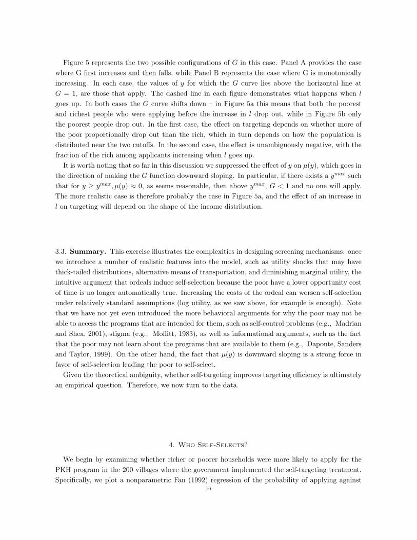
Figure 5 represents the two possible configurations of G in this case. Panel A provides the casewhere G first increases and then falls, while Panel B represents the case where G is monotonicallyincreasing. In each case, the values of y for which the G curve lies above the horizontal line atG = 1, are those that apply. The dashed line in each figure demonstrates what happens when l

goes up. In both cases the G curve shifts down – in Figure 5a this means that both the poorestand richest people who were applying before the increase in l drop out, while in Figure 5b onlythe poorest people drop out. In the first case, the effect on targeting depends on whether more ofthe poor proportionally drop out than the rich, which in turn depends on how the population isdistributed near the two cutoffs. In the second case, the effect is unambiguously negative, with thefraction of the rich among applicants increasing when l goes up.

It is worth noting that so far in this discussion we suppressed the effect of y on µ(y), which goes inthe direction of making the G function downward sloping. In particular, if there exists a ymax suchthat for y � ymax, µ(y) ⇡ 0, as seems reasonable, then above ymax, G < 1 and no one will apply.The more realistic case is therefore probably the case in Figure 5a, and the effect of an increase inl on targeting will depend on the shape of the income distribution.

3.3. Summary. This exercise illustrates the complexities in designing screening mechanisms: oncewe introduce a number of realistic features into the model, such as utility shocks that may havethick-tailed distributions, alternative means of transportation, and diminishing marginal utility, theintuitive argument that ordeals induce self-selection because the poor have a lower opportunity costof time is no longer automatically true. Increasing the costs of the ordeal can worsen self-selectionunder relatively standard assumptions (log utility, as we saw above, for example is enough). Notethat we have not yet even introduced the more behavioral arguments for why the poor may not beable to access the programs that are intended for them, such as self-control problems (e.g., Madrianand Shea, 2001), stigma (e.g., Moffitt, 1983), as well as informational arguments, such as the factthat the poor may not learn about the programs that are available to them (e.g., Daponte, Sandersand Taylor, 1999). On the other hand, the fact that µ(y) is downward sloping is a strong force infavor of self-selection leading the poor to self-select.

Given the theoretical ambiguity, whether self-targeting improves targeting efficiency is ultimatelyan empirical question. Therefore, we now turn to the data.

4. Who Self-Selects?

We begin by examining whether richer or poorer households were more likely to apply for thePKH program in the 200 villages where the government implemented the self-targeting treatment.Specifically, we plot a nonparametric Fan (1992) regression of the probability of applying against

16

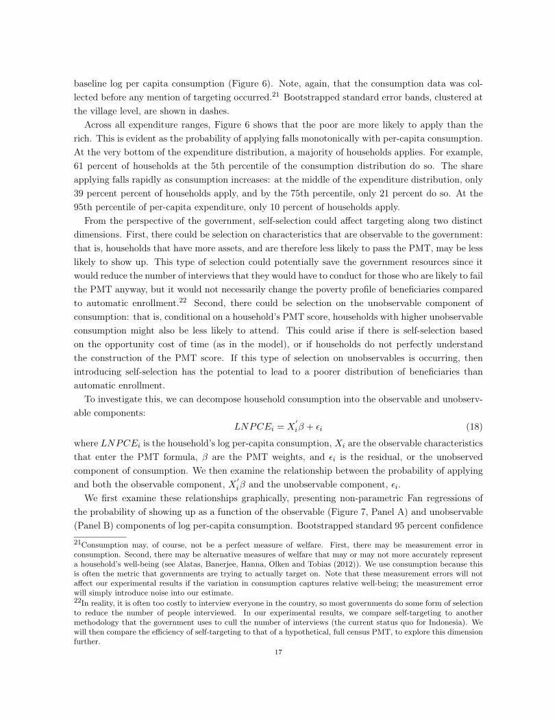
baseline log per capita consumption (Figure 6). Note, again, that the consumption data was col-lected before any mention of targeting occurred.21 Bootstrapped standard error bands, clustered atthe village level, are shown in dashes.

Across all expenditure ranges, Figure 6 shows that the poor are more likely to apply than therich. This is evident as the probability of applying falls monotonically with per-capita consumption.At the very bottom of the expenditure distribution, a majority of households applies. For example,61 percent of households at the 5th percentile of the consumption distribution do so. The shareapplying falls rapidly as consumption increases: at the middle of the expenditure distribution, only39 percent percent of households apply, and by the 75th percentile, only 21 percent do so. At the95th percentile of per-capita expenditure, only 10 percent of households apply.

From the perspective of the government, self-selection could affect targeting along two distinctdimensions. First, there could be selection on characteristics that are observable to the government:that is, households that have more assets, and are therefore less likely to pass the PMT, may be lesslikely to show up. This type of selection could potentially save the government resources since itwould reduce the number of interviews that they would have to conduct for those who are likely to failthe PMT anyway, but it would not necessarily change the poverty profile of beneficiaries comparedto automatic enrollment.22 Second, there could be selection on the unobservable component ofconsumption: that is, conditional on a household’s PMT score, households with higher unobservableconsumption might also be less likely to attend. This could arise if there is self-selection basedon the opportunity cost of time (as in the model), or if households do not perfectly understandthe construction of the PMT score. If this type of selection on unobservables is occurring, thenintroducing self-selection has the potential to lead to a poorer distribution of beneficiaries thanautomatic enrollment.

To investigate this, we can decompose household consumption into the observable and unobserv-able components:

LNPCEi

= X0i

� + ✏i

(18)

where LNPCEi

is the household’s log per-capita consumption, Xi

are the observable characteristicsthat enter the PMT formula, � are the PMT weights, and ✏

i

is the residual, or the unobservedcomponent of consumption. We then examine the relationship between the probability of applyingand both the observable component, X 0

i

� and the unobservable component, ✏i

.We first examine these relationships graphically, presenting non-parametric Fan regressions of

the probability of showing up as a function of the observable (Figure 7, Panel A) and unobservable(Panel B) components of log per-capita consumption. Bootstrapped standard 95 percent confidence

21Consumption may, of course, not be a perfect measure of welfare. First, there may be measurement error inconsumption. Second, there may be alternative measures of welfare that may or may not more accurately representa household’s well-being (see Alatas, Banerjee, Hanna, Olken and Tobias (2012)). We use consumption because thisis often the metric that governments are trying to actually target on. Note that these measurement errors will notaffect our experimental results if the variation in consumption captures relative well-being; the measurement errorwill simply introduce noise into our estimate.22In reality, it is often too costly to interview everyone in the country, so most governments do some form of selectionto reduce the number of people interviewed. In our experimental results, we compare self-targeting to anothermethodology that the government uses to cull the number of interviews (the current status quo for Indonesia). Wewill then compare the efficiency of self-targeting to that of a hypothetical, full census PMT, to explore this dimensionfurther.

17

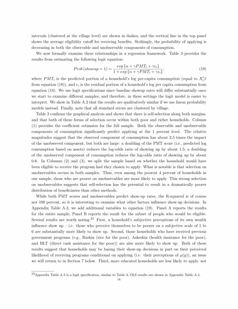
intervals (clustered at the village level) are shown in dashes, and the vertical line in the top panelshows the average eligibility cutoff for receiving benefits. Strikingly, the probability of applying isdecreasing in both the observable and unobservable components of consumption.

We now formally examine these relationships in a regression framework. Table 3 provides theresults from estimating the following logit equation:

Prob (showup = 1) =exp {↵+ �PMT

i

+ �✏i

}1 + exp {↵+ �PMT

i

+ �✏i

} , (19)

where PMTi

is the predicted portion of a household’s log per-capita consumption (equal to X 0i

�

from equation (18)), and ✏i

is the residual portion of a household’s log per capita consumption fromequation (18). We use logit specifications since baseline showup rates will differ substantially oncewe start to examine different samples, and therefore, in these settings the logit model is easier tointerpret. We show in Table A.2 that the results are qualitatively similar if we use linear probabilitymodels instead. Finally, note that all standard errors are clustered by village.

Table 3 confirms the graphical analysis and shows that there is self-selection along both margins,and that both of these forms of selection occur within both poor and richer households. Column(1) provides the coefficient estimates for the full sample. Both the observable and unobservablecomponents of consumption significantly predict applying at the 1 percent level. The relativemagnitudes suggest that the observed component of consumption has about 2.5 times the impactof the unobserved component, but both are large: a doubling of the PMT score (i.e., predicted logconsumption based on assets) reduces the log-odds ratio of showing up by about 1.5; a doublingof the unobserved component of consumption reduces the log-odds ratio of showing up by about0.6. In Columns (2) and (3), we split the sample based on whether the household would havebeen eligible to receive the program had they chosen to apply. What is notable is that selection onunobservables occurs in both samples. Thus, even among the poorest 4 percent of households inour sample, those who are poorer on unobservables are more likely to apply. This strong selectionon unobservables suggests that self-selection has the potential to result in a dramatically poorerdistribution of beneficiaries than other methods.

While both PMT scores and unobservables predict show-up rates, the R-squared is of coursenot 100 percent, so it is interesting to examine what other factors influence show-up decisions. InAppendix Table A.3, we add additional variables to equation (19). Panel A reports the resultsfor the entire sample; Panel B reports the result for the subset of people who would be eligible.Several results are worth noting.23 First, a household’s subjective perceptions of its own wealthinfluence show up – i.e. those who perceive themselves to be poorer on a subjective scale of 1 to6 are substantially more likely to show up. Second, those households who have received previousgovernment programs (e.g., Raskin (rice for the poor), Askeskin (health insurance for the poor),and BLT (direct cash assistance for the poor)) are also more likely to show up. Both of theseresults suggest that households may be basing their show-up decisions in part on their perceivedlikelihood of receiving programs conditional on applying (i.e. their perceptions of µ(y)), an issuewe will return to in Section 7 below. Third, more educated households are less likely to apply, not

23Appendix Table A.3 is a logit specification, similar to Table 3; OLS results are shown in Appendix Table A.4.18

more, suggesting that education is not a constraint on understanding program application rules inthis context.

5. Comparing Self-Selection and Automatic Enrollment

The self-targeting treatment generated considerable self-selection, and yet only about 60 percentof the poorest group showed up, suggesting that there was significant exclusion error. However, itis not clear that we should be comparing self-targeting to the theoretical ideal of no error because,in reality, it is very costly for the government to collect consumption data for each and everyhousehold. Instead, the government’s choice is often to conduct self-targeting or to conduct analternative targeting methodology.24 Therefore, in Section 5.1, we compare self-targeting againstthe real government procedure, which consists of an automatic enrollment for those who pass aproxy-means test among those selected to be interviewed by the government and local communities.Next, in Section 5.2, we additionally compare self-selection against a hypothetical exercise where weuse the data that we have collected independently to predict selection if the automatic enrollment,based on the proxy-means test, was implemented universally.

5.1. Experimental Comparison of Self-Targeting with Status Quo Targeting. In this sec-tion, we test whether the types of individuals selected under self-targeting and automatic enrollment(the current status quo procedure of the Indonesian government) differ. To do so, we compare thedistribution of beneficiaries in the 200 villages randomized to receive the self-targeting treatmentwith the 200 villages randomized to receive the automatic enrollment treatment. Given the random-ization, the distribution of beneficiaries and the probability of receiving benefits should be identicalin the two sets of villages absent the difference in targeting, so we can ascribe the differences that weobserve between the two sets of villages to the differences in targeting methodologies (see AppendixTable A.1).

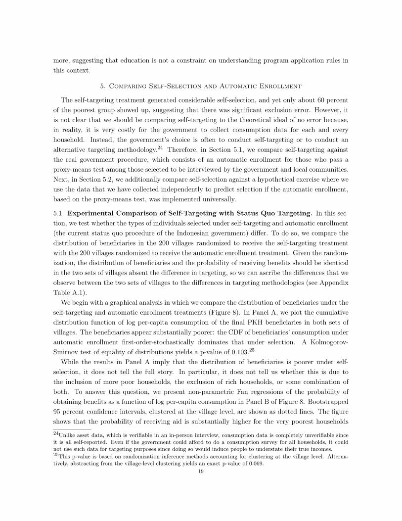
We begin with a graphical analysis in which we compare the distribution of beneficiaries under theself-targeting and automatic enrollment treatments (Figure 8). In Panel A, we plot the cumulativedistribution function of log per-capita consumption of the final PKH beneficiaries in both sets ofvillages. The beneficiaries appear substantially poorer: the CDF of beneficiaries’ consumption underautomatic enrollment first-order-stochastically dominates that under selection. A Kolmogorov-Smirnov test of equality of distributions yields a p-value of 0.103.25

While the results in Panel A imply that the distribution of beneficiaries is poorer under self-selection, it does not tell the full story. In particular, it does not tell us whether this is due tothe inclusion of more poor households, the exclusion of rich households, or some combination ofboth. To answer this question, we present non-parametric Fan regressions of the probability ofobtaining benefits as a function of log per-capita consumption in Panel B of Figure 8. Bootstrapped95 percent confidence intervals, clustered at the village level, are shown as dotted lines. The figureshows that the probability of receiving aid is substantially higher for the very poorest households24Unlike asset data, which is verifiable in an in-person interview, consumption data is completely unverifiable sinceit is all self-reported. Even if the government could afford to do a consumption survey for all households, it couldnot use such data for targeting purposes since doing so would induce people to understate their true incomes.25This p-value is based on randomization inference methods accounting for clustering at the village level. Alterna-tively, abstracting from the village-level clustering yields an exact p-value of 0.069.

19

in the self-targeting treatment. For those with log per capita consumption in the bottom 5 percent,i.e. those with log per capita consumption below about 12.33, the probability of receiving benefitsis more than double that in self-targeting: 16 percent of those with log per capita consumption inthe bottom 5 percent receive benefits as compared with just 7 percent in the automatic enrollmenttreatment. This difference is statistically significant at the 5 percent level. While exclusion erroris still very high – even in self-targeting, only 16 percent of these very poor households receivedbenefits, meaning that 84 percent were excluded – the rate of receiving benefits is 4 times higherthan the overall rate of 4 percent of households in the sample who receive benefits, and double whatit is in the status quo, automatic enrollment villages.

Conversely, households at higher consumption levels are substantially more likely to receive ben-efits in the automatic enrollment treatment. Households in the top 50 percent of the per-capitaexpenditure distribution – none of whom should be receiving benefits – are more than twice as likelyto receive benefits in automatic enrollment than in the self-targeting treatment: 2.5 percent of suchhouseholds receive benefits in automatic enrollment compared with 1 percent of such householdsin self-targeting (statistically significant at the 5 percent level). One explanation is that there arealways errors in the PMT formula that allow some fraction of ineligible households to slip throughthe proxy-means test. With self-targeting, however, most of these households do not apply, somany fewer of them slip through. In sum, Figure B suggests that self-targeting both increased theprobability that very poor households received benefits and decreased the probability that richerhouseholds did so, relative to the current status quo.

We now more formally quantify these effects using regression analysis, the results of which are pre-sented in Table 4. In Column (1), we compare the difference in average log per capita consumptionof the beneficiary populations (LNPCE

vi

) in the two treatments, by estimating by OLS:

LNPCEvi

= ↵+ �SELFv

+ #vi

, (20)

where SELFv

is a dummy for village v being in the self-targeting treatment, and #vi

is the errorterm. Standard errors are clustered by village. We estimate this model directly (Panel A) and withstratum fixed effects (Panel B). Note that this is the regression equivalent of comparing the meansof the two distributions shown in Panel A of Figure 8. As suggested by the figures, the regressionanalysis confirms that beneficiaries are substantially poorer under self-selection: Column (1) ofPanel A reports that per-capita consumption of beneficiaries is is 21 percent lower in self-targetingas compared to automatic enrollment (significant at the 1 percent level). Including stratum fixedeffects (Panel B), the difference becomes 11 percent, and the p-value increases to 0.14.26

To increase our precision of the difference in consumption levels of beneficiaries, as discussedabove, we did an interim midline survey after the targeting was complete, but before programbeneficiary status had been announced or benefits had begun, in which we oversampled beneficiariesin both PMT and self-targeting villages. In Column (2), we compare log per-capita consumption ofbeneficiaries in the two treatments, including both the 159 beneficiaries from our baseline sample

26In general, one would expect stratum fixed effects to improve precision. However, in the regressions where we onlyconsider beneficiaries, we have so few observations (159 observations), and hence so few observations per stratum, thatincluding the fixed effects effectively drops many whole strata from the analysis, dramatically diminishing statisticalpower.

20

and the additional 745 beneficiaries we oversampled in the midline. Since the average level ofconsumption may be different in these two survey rounds (for example due to seasonality), weinclude a dummy variable for the survey round in which the data was collected. The results inColumn 2 are similar in magnitude but more precisely estimated: self-targeting selects beneficiarieswho are 18 to 19 percent poorer than those selected by the PMT treatment (statistically significantat the 1 percent level).

In Column 3 of Table 4, we examine the probability of getting benefits (Prob (BENEFITvi

= 1))across the treatments for different groups. Specifically, we provide estimates from the following logitmodel:

Prob (BENEFITvi

= 1) =exp {↵+ �SELF

v

+ �LNPCEvi

+ ⌘SELFv

⇥ LNPCEvi

}1 + exp {↵+ �SELF

v

+ �LNPCEvi

+ ⌘SELFv

⇥ LNPCEvi

} . (21)

The coefficient of interest is the coefficient ⌘ on SELFv

⇥ LNPCEvi

, which captures the degreeto which there is differential targeting in the self-targeting treatment as compared with automaticenrollment (the omitted category).27 The results confirm the overall story shown in Panel B ofFigure 8: the coefficient on ⌘ is negative, large in magnitude, and statistically significant. Thisimplies that there is much stronger targeting by consumption in the self-targeting treatment thanin the automatic enrollment treatment. The magnitudes suggest that targeting is twice as strongin self-targeting: the estimates in Panel A imply that doubling consumption decreases the log-oddsof receiving benefits by 0.70 in automatic enrollment, whereas it decreases the log-odds of receivingbenefits by 1.37 in self-targeting.

In Columns (4) - (6), we examine alternative dependent variables to quantify the types of inclusionand exclusion error shown in Panel B of Figure 8. In Column (4) we define the overall error rate as adummy that is equal to 1 if either exclusion error (failing to give benefits to a very poor household)or inclusion error (giving benefits to a non-very poor household) takes place. We find that thelog-odds ratio of making an error is about 0.2 lower under self-targeting (p-values of 0.08 withoutstratum fixed effects and 0.11 with stratum fixed effects). Column (5) examines exclusion error,defined as a dummy for a very poor household failing to receive benefits. The results in the tablesuggest that the log-odds of such households being excluded (i.e., failing to get benefits) are between0.55 and 0.71 lower in self-selection, though these results are not statistically significant (p-valuesof 0.18 and 0.15, respectively). Likewise, inclusion error, defined as a non-very poor household thatdoes receive benefits, is lower in self-targeting, and statistically significant in the specification withstratum fixed effects (Column (6); p-values 0.14 and 0.08, respectively).

On net, the non-parametric and parametric results combine to paint a clear picture: self-targetingleads to a poorer distribution of beneficiaries, both because the poor are more likely to receivebenefits and because richer households are less likely to receive benefits.

27We use logit models because the baseline benefit rate differs substantially by per-capita expenditure, so proportionalmodels make more sense. Stratum fixed effects are also much more effective in proportional models given thesubstantially different poverty levels across strata. Appendix Table (A.5) shows that the OLS version of the sameresults are qualitatively similar, and if anything, show slightly higher levels of statistical significance. We clusterthe standard errors in models with no fixed effects, and all OLS specifications, by village. For the conditional logitmodels where we include stratum fixed effects, for computational reasons we cluster fixed effects by stratum, whichis more conservative (one stratum contains multiple villages).

21

5.2. Comparing Self-Targeting to a Hypothetical Universal Automatic Enrollment Treat-ment. In the automatic enrollment procedure, not all households were considered for enrollment.Instead, as discussed in Section 2.3.1, households only received the full PMT interview if they passedan initial set of screens. These pre-screening criteria were designed to save the government the costof having to conduct a complete long-form census of every household in the country every time itwanted to select beneficiaries. On net, as shown in Table 2, about 34 percent of households in thevillage received the full PMT interview, which is roughly comparable to the share of households whoself-select to be interviewed in the self-targeting treatment. Even though the government explicitlyseeks to interview the poorest by targeting anyone who has ever taken part in a poverty-relatedprogram in the past supplemented by those that local officials think may be eligible, the fact thatself-targeting improved inclusion error relative to the PMT treatment suggests that the governmentmay not always be targeting the right people to interview. This could be the case, for example, ifmany of the very poorest rarely come in contact with government officials, so officialsdo not realizethey are present and hence are not included on the survey list.

Comparing self-targeting against the current procedure is interesting because it provides informa-tion on the different methods that are realistically within a government’s choice set. However, it isalso interesting to ask how self-targeting performs relative to a PMT procedure that does not havethe pre-screening that occurs in the actual procedure. While this is less realistic (i.e., it is too costlyto actually be conducted by the government), it provides us with a greater understanding of themargins through which self-selection occurs. Thus, in this section, we assume, hypothetically, thatthe government had conducted the full PMT interview on everyone in the community. Recalling thedecomposition of who selects to apply in the self-targeting treatment in Section 4 into selection onobservables and selection on unobservables, we know a priori that self-targeting will perform worsethan universal automatic enrollment with respect to selection on observables, because by definitionuniversal automatic enrollment picks up 100 percent of households with PMT scores less than thecutoff whereas self-targeting limits the beneficiaries to a subset of those who chose to apply. How-ever, it is still possible that self-selection could still out-perform universal automatic enrollment onnet if the selection on unobservables is sufficiently large.

To simulate what would have happened in universal automatic enrollment, we use our baselinedata to construct PMT scores for those households not interviewed by the government as part of thePMT process. That is, for those households who were not interviewed as part of the real PMT treat-ment, we assume that they would have received benefits if their PMT score (according to the assetdata we collected in our baseline survey) was below the threshold required to receive the program.We then repeat the same analysis in Figure 8 and Table 4, but instead of comparing self-targeting tothe actual automatic enrollment treatment, we compare it to the constructed hypothetical universalautomatic enrollment procedure.

The results are shown graphically in Figure 9 and in regression form in Table 5. Panel A ofFigure 9 shows that the distribution of beneficiaries still looks poorer in self-selection than in thehypothetical universal automatic enrollment, though the difference between the two distributionsis no longer statistically significant (p-value from the Kolomogorov-Smirnov test of equality ofdistributions, with randomization inference to cluster at village level, is 0.29). Panel B of Figure 9

22

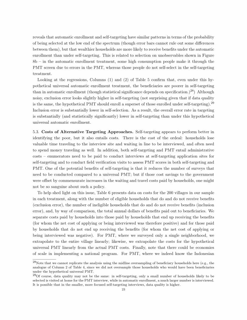
reveals that automatic enrollment and self-targeting have similar patterns in terms of the probabilityof being selected at the low end of the spectrum (though error bars cannot rule out some differencesbetween them), but that wealthier households are more likely to receive benefits under the automaticenrollment than under self-targeting. This is related to selection on unobservables shown in Figure8b – in the automatic enrollment treatment, some high consumption people make it through thePMT screen due to errors in the PMT, whereas those people do not self-select in the self-targetingtreatment.

Looking at the regressions, Columns (1) and (2) of Table 5 confirm that, even under this hy-pothetical universal automatic enrollment treatment, the beneficiaries are poorer in self-targetingthan in automatic enrollment (though statistical significance depends on specification.)28) Althoughnoisy, exclusion error looks slightly higher in self-targeting (not surprising given that if data qualityis the same, the hypothetical PMT should enroll a superset of those enrolled under self-targeting).29

Inclusion error is substantially lower in self-selection. As a result, the overall error rate in targetingis substantially (and statistically significantly) lower in self-targeting than under this hypotheticaluniversal automatic enrollment.

5.3. Costs of Alternative Targeting Approaches. Self-targeting appears to perform better inidentifying the poor, but it also entails costs. There is the cost of the ordeal: households losevaluable time traveling to the interview site and waiting in line to be interviewed, and often needto spend money traveling as well. In addition, both self-targeting and PMT entail administrativecosts – enumerators need to be paid to conduct interviews at self-targeting application sites forself-targeting and to conduct field verification visits to assess PMT scores in both self-targeting andPMT. One of the potential benefits of self-targeting is that it reduces the number of surveys thatneed to be conducted compared to a universal PMT; but if those cost savings to the governmentwere offset by commensurate increases in the waiting and travel costs paid by households, one mightnot be so sanguine about such a policy.

To help shed light on this issue, Table 6 presents data on costs for the 200 villages in our samplein each treatment, along with the number of eligible households that do and do not receive benefits(exclusion error), the number of ineligible households that do and do not receive benefits (inclusionerror), and, by way of comparison, the total annual dollars of benefits paid out to beneficiaries. Weseparate costs paid by households into those paid by households that end up receiving the benefits(for whom the net cost of applying or being interviewed was therefore positive) and for those paidby households that do not end up receiving the benefits (for whom the net cost of applying orbeing interviewed was negative). For PMT, where we surveyed only a single neighborhood, weextrapolate to the entire village linearly; likewise, we extrapolate the costs for the hypotheticaluniversal PMT linearly from the actual PMT costs. Finally, note that there could be economiesof scale in implementing a national program. For PMT, where we indeed know the Indonesian

28Note that we cannot replicate the analysis using the midline oversampling of beneficiary households here (e.g., theanalogue of Column 2 of Table 4, since we did not oversample those households who would have been beneficiariesunder the hypothetical universal PMT.29Of course, data quality may not be the same: in self-targeting, only a small number of households likely to beselected is visited at home for the PMT interview, while in automatic enrollment, a much larger number is interviewed.It is possible that in the smaller, more focused self-targeting interviews, data quality is higher.

23

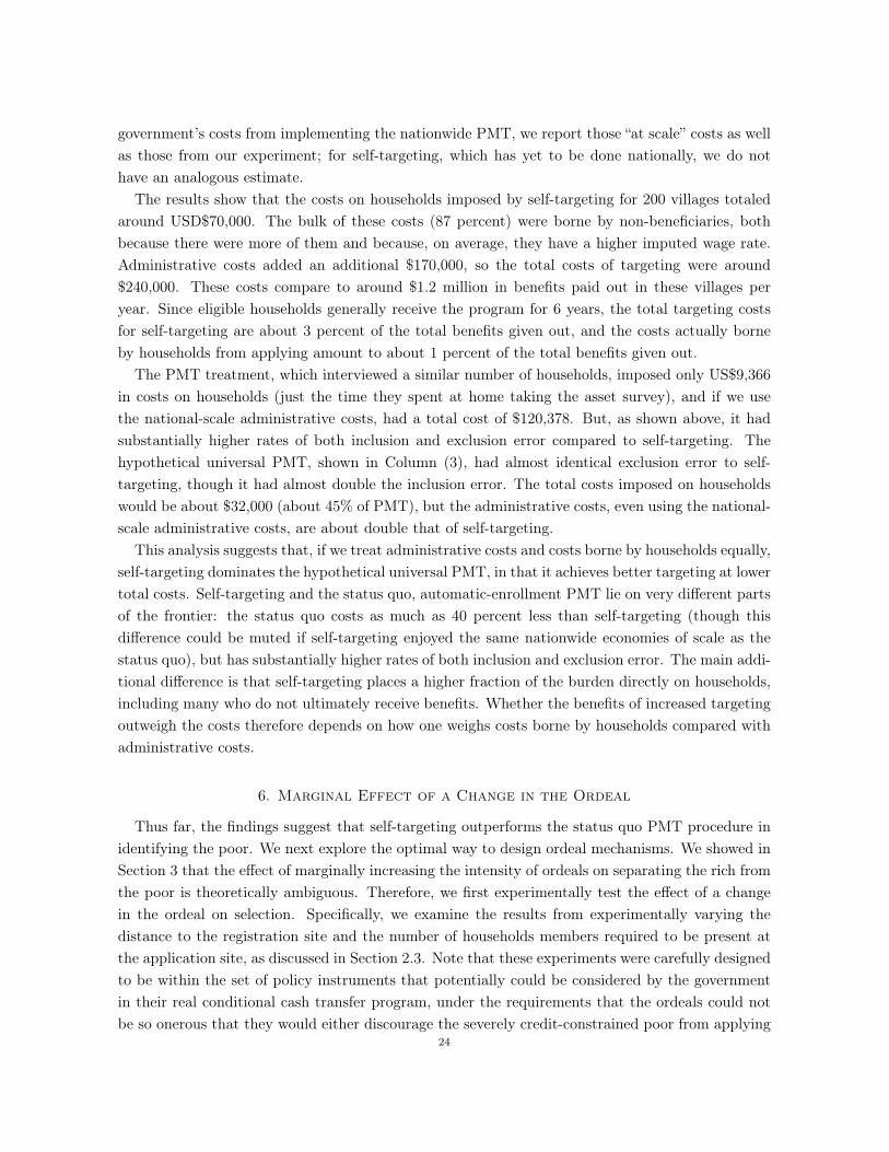
government’s costs from implementing the nationwide PMT, we report those “at scale” costs as wellas those from our experiment; for self-targeting, which has yet to be done nationally, we do nothave an analogous estimate.

The results show that the costs on households imposed by self-targeting for 200 villages totaledaround USD$70,000. The bulk of these costs (87 percent) were borne by non-beneficiaries, bothbecause there were more of them and because, on average, they have a higher imputed wage rate.Administrative costs added an additional $170,000, so the total costs of targeting were around$240,000. These costs compare to around $1.2 million in benefits paid out in these villages peryear. Since eligible households generally receive the program for 6 years, the total targeting costsfor self-targeting are about 3 percent of the total benefits given out, and the costs actually borneby households from applying amount to about 1 percent of the total benefits given out.

The PMT treatment, which interviewed a similar number of households, imposed only US$9,366in costs on households (just the time they spent at home taking the asset survey), and if we usethe national-scale administrative costs, had a total cost of $120,378. But, as shown above, it hadsubstantially higher rates of both inclusion and exclusion error compared to self-targeting. Thehypothetical universal PMT, shown in Column (3), had almost identical exclusion error to self-targeting, though it had almost double the inclusion error. The total costs imposed on householdswould be about $32,000 (about 45% of PMT), but the administrative costs, even using the national-scale administrative costs, are about double that of self-targeting.

This analysis suggests that, if we treat administrative costs and costs borne by households equally,self-targeting dominates the hypothetical universal PMT, in that it achieves better targeting at lowertotal costs. Self-targeting and the status quo, automatic-enrollment PMT lie on very different partsof the frontier: the status quo costs as much as 40 percent less than self-targeting (though thisdifference could be muted if self-targeting enjoyed the same nationwide economies of scale as thestatus quo), but has substantially higher rates of both inclusion and exclusion error. The main addi-tional difference is that self-targeting places a higher fraction of the burden directly on households,including many who do not ultimately receive benefits. Whether the benefits of increased targetingoutweigh the costs therefore depends on how one weighs costs borne by households compared withadministrative costs.

6. Marginal Effect of a Change in the Ordeal

Thus far, the findings suggest that self-targeting outperforms the status quo PMT procedure inidentifying the poor. We next explore the optimal way to design ordeal mechanisms. We showed inSection 3 that the effect of marginally increasing the intensity of ordeals on separating the rich fromthe poor is theoretically ambiguous. Therefore, we first experimentally test the effect of a changein the ordeal on selection. Specifically, we examine the results from experimentally varying thedistance to the registration site and the number of households members required to be present atthe application site, as discussed in Section 2.3. Note that these experiments were carefully designedto be within the set of policy instruments that potentially could be considered by the governmentin their real conditional cash transfer program, under the requirements that the ordeals could notbe so onerous that they would either discourage the severely credit-constrained poor from applying

24

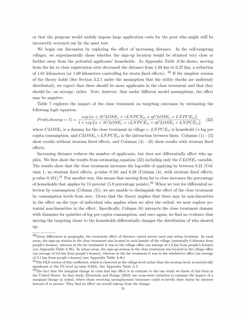
or that the program would unduly impose large application costs for the poor who might still beincorrectly screened out by the asset test.

We begin our discussion by exploring the effect of increasing distance. In the self-targetingvillages, we experimentally chose whether the sign-up location would be situated very close orfurther away from the potential applicants’ households. As Appendix Table A.9a shows, movingfrom the far to close registration sites decreased the distance from 1.88 km to 0.27 km; a reductionof 1.61 kilometers (or 1.69 kilometers controlling for strata fixed effects). 30 If the simplest versionof the theory holds (See Section 3.2.1 under the assumption that the utility shocks are uniformlydistributed), we expect that there should be more applicants in the close treatment and that theyshould be, on average, richer. Note, however, that under different model assumptions, the effectmay be negative.

Table 7 explores the impact of the close treatment on targeting outcomes by estimating thefollowing logit equation:

Prob (showup = 1) =exp {↵+ �CLOSE

v

+ �LNPCEvi

+ ⌘CLOSEv

⇥ LNPCEvi

}1 + exp {↵+ �CLOSE

v

+ �LNPCEvi

+ ⌘CLOSEv

⇥ LNPCEvi

} (22)

where CLOSEv

is a dummy for the close treatment in village v, LNPCEvi

is household i’s log percapita consumption, and CLOSE

v

⇥LNPCEvi

is the interaction between them. Columns (1) - (3)show results without stratum fixed effects, and Columns (4) - (6) show results with stratum fixedeffects.

Increasing distance reduces the number of applicants, but does not differentially affect who ap-plies. We first show the results from estimating equation (22) including only the CLOSE

v

variable.The results show that the close treatment increases the log-odds of applying by between 0.21 (Col-umn 1, no stratum fixed effects, p-value 0.16) and 0.28 (Column (4), with stratum fixed effects,p-value 0.101).31 Put another way, this means that moving from far to close increases the percentageof households that applies by 15 percent (5.8 percentage points).32 When we test for differential se-lection by consumption (Column (5)), we are unable to distinguish the effect of the close treatmentby consumption levels from zero. Given that the theory implies that there may be non-linearitiesin the effect on the type of individual who applies when we alter the ordeal, we next explore po-tential non-linearities in the effect. Specifically, Column (6) interacts the close treatment dummywith dummies for quintiles of log per-capita consumption, and once again, we find no evidence thatmoving the targeting closer to the households differentially changes the distribution of who showedup.

30Given differences in geography, the treatment effect of distance varied across rural and urban locations. In ruralareas, the sign-up station in the close treatment was located in each hamlet of the village (essentially 0 distance frompeople’s houses), whereas in the far treatment it was in the village office (an average of 1.2 km from people’s houses)(see Appendix Table A.9b). In urban areas, the sign-up station in the close treatment was located in the village office(an average of 0.8 km from people’s houses), whereas in the far treatment it was in the subdistrict office (an averageof 3.1 km from people’s houses) (see Appendix Table A.9c).31The OLS version of this coefficient, which is clustered at the village level rather than the stratum level, is statisticallysignificant at the 5% level (p-value 0.024). See Appendix Table A.7.32The fact that the marginal change in costs had any effect is in contrast to the one study we know of this form inthe United States. In that study, Ebenstein and Stange (2010) use cross-state variation to examine the impact of amarginal change in ordeal, where those receiving unemployment insurance could re-certify their status by internetinstead of in person. They find no effect on overall takeup from the change.

25

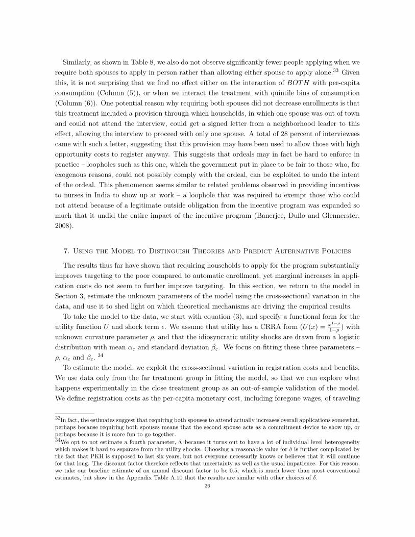
Similarly, as shown in Table 8, we also do not observe significantly fewer people applying when werequire both spouses to apply in person rather than allowing either spouse to apply alone.33 Giventhis, it is not surprising that we find no effect either on the interaction of BOTH with per-capitaconsumption (Column (5)), or when we interact the treatment with quintile bins of consumption(Column (6)). One potential reason why requiring both spouses did not decrease enrollments is thatthis treatment included a provision through which households, in which one spouse was out of townand could not attend the interview, could get a signed letter from a neighborhood leader to thiseffect, allowing the interview to proceed with only one spouse. A total of 28 percent of intervieweescame with such a letter, suggesting that this provision may have been used to allow those with highopportunity costs to register anyway. This suggests that ordeals may in fact be hard to enforce inpractice – loopholes such as this one, which the government put in place to be fair to those who, forexogenous reasons, could not possibly comply with the ordeal, can be exploited to undo the intentof the ordeal. This phenomenon seems similar to related problems observed in providing incentivesto nurses in India to show up at work – a loophole that was required to exempt those who couldnot attend because of a legitimate outside obligation from the incentive program was expanded somuch that it undid the entire impact of the incentive program (Banerjee, Duflo and Glennerster,2008).

7. Using the Model to Distinguish Theories and Predict Alternative Policies

The results thus far have shown that requiring households to apply for the program substantiallyimproves targeting to the poor compared to automatic enrollment, yet marginal increases in appli-cation costs do not seem to further improve targeting. In this section, we return to the model inSection 3, estimate the unknown parameters of the model using the cross-sectional variation in thedata, and use it to shed light on which theoretical mechanisms are driving the empirical results.

To take the model to the data, we start with equation (3), and specify a functional form for theutility function U and shock term ✏. We assume that utility has a CRRA form (U(x) = x

1�⇢

1�⇢

) withunknown curvature parameter ⇢, and that the idiosyncratic utility shocks are drawn from a logisticdistribution with mean ↵

"

and standard deviation �"

. We focus on fitting these three parameters –⇢, ↵

"

and �"

. 34

To estimate the model, we exploit the cross-sectional variation in registration costs and benefits.We use data only from the far treatment group in fitting the model, so that we can explore whathappens experimentally in the close treatment group as an out-of-sample validation of the model.We define registration costs as the per-capita monetary cost, including foregone wages, of traveling

33In fact, the estimates suggest that requiring both spouses to attend actually increases overall applications somewhat,perhaps because requiring both spouses means that the second spouse acts as a commitment device to show up, orperhaps because it is more fun to go together.34We opt to not estimate a fourth parameter, �, because it turns out to have a lot of individual level heterogeneitywhich makes it hard to separate from the utility shocks. Choosing a reasonable value for � is further complicated bythe fact that PKH is supposed to last six years, but not everyone necessarily knows or believes that it will continuefor that long. The discount factor therefore reflects that uncertainty as well as the usual impatience. For this reason,we take our baseline estimate of an annual discount factor to be 0.5, which is much lower than most conventionalestimates, but show in the Appendix Table A.10 that the results are similar with other choices of �.

26

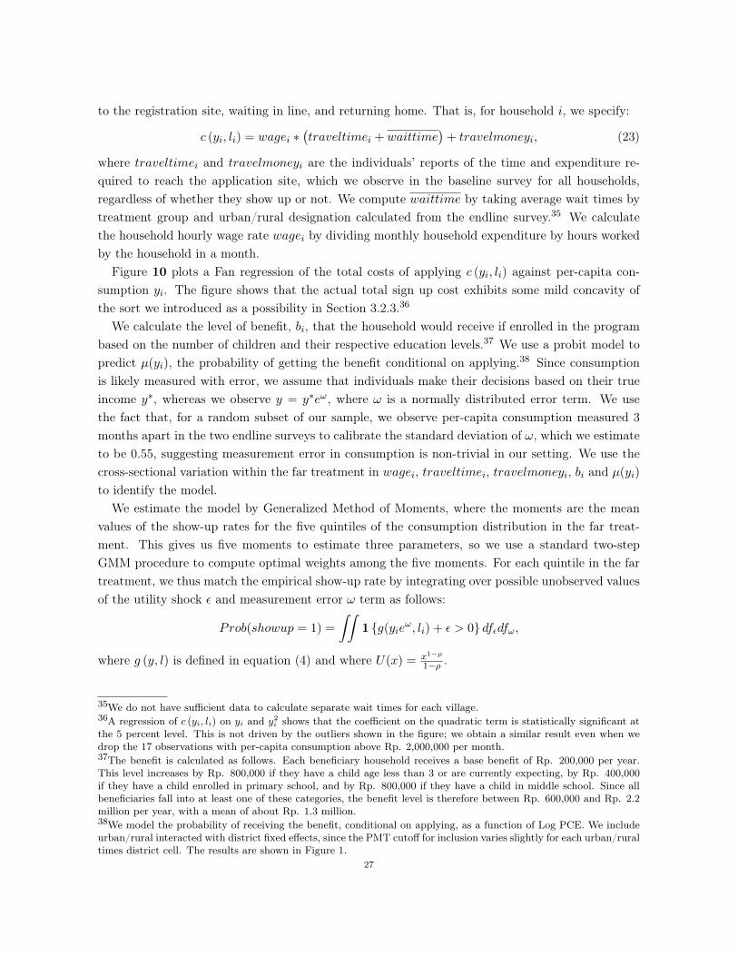
to the registration site, waiting in line, and returning home. That is, for household i, we specify:

c (yi

, li

) = wagei

⇤�traveltime

i

+ waittime�+ travelmoney

i

, (23)

where traveltimei

and travelmoneyi

are the individuals’ reports of the time and expenditure re-quired to reach the application site, which we observe in the baseline survey for all households,regardless of whether they show up or not. We compute waittime by taking average wait times bytreatment group and urban/rural designation calculated from the endline survey.35 We calculatethe household hourly wage rate wage

i

by dividing monthly household expenditure by hours workedby the household in a month.

Figure 10 plots a Fan regression of the total costs of applying c (yi

, li

) against per-capita con-sumption y

i

. The figure shows that the actual total sign up cost exhibits some mild concavity ofthe sort we introduced as a possibility in Section 3.2.3.36

We calculate the level of benefit, bi

, that the household would receive if enrolled in the programbased on the number of children and their respective education levels.37 We use a probit model topredict µ(y

i

), the probability of getting the benefit conditional on applying.38 Since consumptionis likely measured with error, we assume that individuals make their decisions based on their trueincome y⇤, whereas we observe y = y⇤e!, where ! is a normally distributed error term. We usethe fact that, for a random subset of our sample, we observe per-capita consumption measured 3months apart in the two endline surveys to calibrate the standard deviation of !, which we estimateto be 0.55, suggesting measurement error in consumption is non-trivial in our setting. We use thecross-sectional variation within the far treatment in wage

i

, traveltimei

, travelmoneyi

, bi

and µ(yi

)

to identify the model.We estimate the model by Generalized Method of Moments, where the moments are the mean

values of the show-up rates for the five quintiles of the consumption distribution in the far treat-ment. This gives us five moments to estimate three parameters, so we use a standard two-stepGMM procedure to compute optimal weights among the five moments. For each quintile in the fartreatment, we thus match the empirical show-up rate by integrating over possible unobserved valuesof the utility shock ✏ and measurement error ! term as follows:

Prob(showup = 1) =

ZZ1 {g(y

i

e!, li

) + ✏ > 0} df✏

df!

,

where g (y, l) is defined in equation (4) and where U(x) = x

1�⇢

1�⇢

.

35We do not have sufficient data to calculate separate wait times for each village.36A regression of c (yi, li) on yi and y

2i shows that the coefficient on the quadratic term is statistically significant at

the 5 percent level. This is not driven by the outliers shown in the figure; we obtain a similar result even when wedrop the 17 observations with per-capita consumption above Rp. 2,000,000 per month.37The benefit is calculated as follows. Each beneficiary household receives a base benefit of Rp. 200,000 per year.This level increases by Rp. 800,000 if they have a child age less than 3 or are currently expecting, by Rp. 400,000if they have a child enrolled in primary school, and by Rp. 800,000 if they have a child in middle school. Since allbeneficiaries fall into at least one of these categories, the benefit level is therefore between Rp. 600,000 and Rp. 2.2million per year, with a mean of about Rp. 1.3 million.38We model the probability of receiving the benefit, conditional on applying, as a function of Log PCE. We includeurban/rural interacted with district fixed effects, since the PMT cutoff for inclusion varies slightly for each urban/ruraltimes district cell. The results are shown in Figure 1.

27

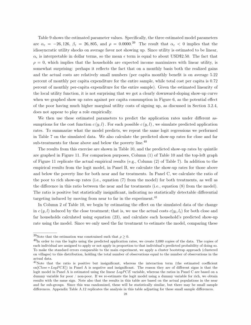
Table 9 shows the estimated parameter values. Specifically, the three estimated model parametersare ↵

"

= �26, 126, �"

= 26, 805, and ⇢ = 0.0000.39 The result that ↵"

< 0 implies that theidiosyncratic utility shocks on average favor not showing up. Since utility is estimated to be linear,↵✏

is interpretable in dollar terms, so the mean ✏ term is equal to about USD$2.50. The fact that⇢ = 0, which implies that the households are expected income maximizers with linear utility, issomewhat surprising: perhaps it reflects the fact that on a monthly basis both the realized gainsand the actual costs are relatively small numbers (per capita monthly benefit is on average 5.22percent of monthly per capita expenditure for the entire sample, while total cost per capita is 0.72percent of monthly per-capita expenditure for the entire sample). Given the estimated linearity ofthe local utility function, it is not surprising that we got a clearly downward-sloping show-up curvewhen we graphed show up rates against per capita consumption in Figure 6, as the potential effectof the poor having much higher marginal utility costs of signing up, as discussed in Section 3.2.4,does not appear to play a role empirically.

We then use these estimated parameters to predict the application rates under different as-sumptions for the cost function c (y, l) . For each possible c (y, l) , we simulate predicted applicationrates. To summarize what the model predicts, we repeat the same logit regressions we performedin Table 7 on the simulated data. We also calculate the predicted show-up rates for close and farsub-treatments for those above and below the poverty line.40

The results from this exercise are shown in Table 10, and the predicted show-up rates by quintileare graphed in Figure 11. For comparison purposes, Column (1) of Table 10 and the top-left graphof Figure 11 replicate the actual empirical results (e.g., Column (2) of Table 7). In addition to theempirical results from the logit model, in Panel B, we calculate the show-up rates for those aboveand below the poverty line for both near and far treatments. In Panel C, we calculate the ratio ofthe poor to rich show-up rates (i.e., equation (7) from the model) for both treatments, as well asthe difference in this ratio between the near and far treatments (i.e., equation (8) from the model).The ratio is positive but statistically insignificant, indicating no statistically detectable differentialtargeting induced by moving from near to far in the experiment.41

In Column 2 of Table 10, we begin by estimating the effect on the simulated data of the changein c (y, l) induced by the close treatment; that is, we use the actual costs c(y

i

, li

) for both close andfar households calculated using equation (23), and calculate each household’s predicted show-uprate using the model. Since we only used the far treatment to estimate the model, comparing these

39Note that the estimation was constrained such that ⇢ � 0.40In order to run the logits using the predicted application rates, we create 3,000 copies of the data. The copies ofeach individual are assigned to apply or not apply in proportion to that individual’s predicted probability of doing so.To make the standard errors comparable to the main experiment, we apply a cluster bootstrap approach (clusteredon villages) to this distribution, holding the total number of observations equal to the number of observations in theactual data.41Note that the ratio is positive but insignificant, whereas the interaction term (the estimated coefficienton[Close ⇤ LogPCE]) in Panel A is negative and insignificant. The reason they are of different signs is that thelogit model in Panel A is estimated using the linear LogPCE variable, whereas the ratios in Panel C are based on adummy variable for poor / non-poor. If we re-estimate the logit model using a dummy variable for rich, we obtainresults with the same sign. Note also that the results in this table are based on the actual populations in the nearand far sub-groups. Since this was randomized, these will be statistically similar, but there may be small sampledifferences. Appendix Table A.12 replicates the analysis in this table adjusting for these small sample differences.

28

simulated show-up rates to actual show-up rates serves as an out-of-sample check of the fit of themodel using the experiment. We bootstrap the standard errors using sample sizes equivalent to ouractual data and with village-level clustering, so that the standard errors reported for the model-generated data are equivalent to those from the actual data. The results in column 2 thus showwhat we would have found had the data from our actual survey been generated by the model.42

Comparing the actual empirical estimates in Column 1 with the estimates on the model-generateddata in Column 2, we find similar results of differential targeting between the treatments. In partic-ular, even though the model seems to over-predict show up rates in the close treatment on average,the small differential effect between rich and poor show up ratios moving from near to far in thesimulated data is not statistically distinguishable from what we actually observe in the experiment(Panel C; p-value 0.602). Consistent with this, the coefficients on the close dummy interacted withlog per capita consumption (⌘ in equation (22)), which is another way of capturing the degree ofdifferential targeting between the close and far treatment, are also statistically indistinguishablebetween the actual experimental data in Column (1) and the simulated data in Column (2) (p-value 0.441). The fact that the model predictions are similar to the experimental findings providesus with greater confidence in the simulation results for alternative cost structures in the followingcolumns.43 A comparison of model fit can be seen by comparing the actual show up rates by quintileand treatment in the top-left of Figure 11 with the model’s predicted show up rates by quintile andtreatment in the top-middle of Figure 11.

7.1. Distinguishing Alternate Theories. Interestingly, even though there is strong evidenceof self-selection (the poor are much more likely to show up than the rich, both on observablesand unobservables), both the experiment and the model show no statistically significant marginalincrease in the targeting ratio from increasing the severity of the ordeal (i.e., moving from neartreatment to far). We can use the model to help understand why this is not occurring, and inparticular, examine the various mechanisms outlined in the model in Section 3.

Shocks. One possible explanation developed in the theory section is that, if the distribution ofshocks does not have the monotone hazard rate property, it is possible that targeting could getworse as you increase distance, because the density of poor people induced to drop out by a highermarginal change is higher than the density of richer people (see Section 3.2.2). However, the versionof the structural model we estimate and use in Column (2) uses logit shocks, which do have the

42Over the last few years there have been several papers in the development literature that similarly use a well-identified randomized or natural experiment to provide a check of model fit. These include Todd and Wolpin (2006),Kaboski and Townsend (2011) and Duflo, Hanna and Ryan (2012). More generally, the idea of hold out samples forvalidation has been used in several papers in the broader applied micro literature, staring at least with McFadden(1977); see for example, Wise (1985), Lise, Seitz and Smith (2004), Keane and Mott (1998), Keane, Todd andWolpin (2011). Other papers which combine structural methods and experimental data (without using one of theexperimental groups for out of sample validation) include Attanasio, Meghir and Santiago (2012), Einav et al. (2013)and Ferrall (2010).43The one aspect of the model that does not match is that the predicted show-up rates for those below the povertyline are actually higher in the far treatment than in the near treatment (69 percent vs 67 percent). We have verifiedthat this is not due to the model, but rather due to small-sample differences in the expected benefits from obtainingthe program among the poor in these two samples. In particular, the poor in the far group have (statisticallyinsignificantly) more middle schoolers than the poor in the near group, which leads to higher show-up rates. If wesimulate the impact of moving from far to close on the exact same group of beneficiaries, we indeed would obtainlower show-up rates in far than in close in both rich and poor samples. See Appendix Table A.12.

29

monotone hazard rate property, yet still replicates the experimental findings. This suggests thatthe distribution of shocks alone is not the problem.

However, the magnitude of the shocks may explain why the response is so low. Examiningequation (8), which showed the derivative of the show-up ratio with respect to a change in distancel, one can see that increasing the variance of the shocks, which would lower the PDF f at themargin for both rich and poor, would dampen the responsiveness to a marginal increase in ordeals.To assess quantitatively whether this is important, in Column (3) we re-simulate the model wherewe cut the standard deviation of the shocks ✏ in half. Doing so increases the point estimate of theimpact of moving from close to far on the poor/rich show-up ratio – from 0.314 in the base-casemodel to 0.470 – but it would still not have been enough to be statistically detectable. In Column(4) we shut off the shocks entirely, so that everyone for whom g(y, l) > 0 shows up. This increasesthe estimated impact on the show-up ratio to 0.584, but again, it would not have been enough tobe statistically detectable.

Curvature in the Utility Function. Another possible explanation given by the theory is that theremay be curvature in the utility function, so that even though the marginal monetary cost of higherdistance is greater for the rich, the monetary utility cost is greater for the poor (see Section 3.2.4).However, when we estimated the structural model, the found that the model was best fit with linearutility (i.e. ⇢ = 0), suggesting that this is not an important part of the explanation in our setting.44

Different Travel Technologies s. The third explanation suggested by the model is that there aredifferent transportation technologies used by the poor and the rich, so that the marginal monetarycost of distance is smaller for the rich (see Section 3.2.3). Figure 10 showed that this might be apossible explanation in the data, as the total costs of travel do appear to be concave in per-capitaconsumption. To investigate whether this explains the lack of differential selection in response to anincrease in distance, we use the model to generate simulated show up rates under the counterfactualthat the poor and the rich use the same travel technology. To do so, we model travel costs (timeand money) as a function of distance. Treating urban and rural populations separately, we regressreported monetary costs and reported travel time to the close and far registration places on quadraticfunctions of distance. We then use these predicted average travel costs – which by construction nolonger allow richer households to use different transportation technologies – for all households, andre-calculate total registration costs c (y, l). We then re-estimate the logit regressions and calculatethe show-up rates for the simulated data using these costs instead of the actual costs. Column (5)reports the results, which appear similar to the experimental findings (p-value 0.449 in Panel A;p-value of 0.624 in Panel C). The fact that the results are virtually unchanged when everyone isconstrained to use similar transportation technologies suggests that the lack of differential selectionbetween close and far is not being driven by the fact that the rich and poor use different transporttechnologies. The predicted show-up rates using the same transport technology are shown in thetop right of Figure 11 and confirm that technology is not the main issue.

Probability of Receiving Benefits. A final explanation is that most of the selection we observe inSection 4 is being driven by the fact that households anticipate that µ(y), the probability of receiving

44Appendix Figure A.1 shows the actual model fit, and alternatives where we impose higher values of ⇢. As is evidentfrom the Figure, imposing higher values of ⇢ leads to a more convex relationship between show-up rates and incomequintile than we observe in the data.

30

benefits conditional on showing up, is downward sloping in income.45 To gauge the magnitude ofthat effect, in Column (6), we simulate what would happen if, instead of using the actual empiricalµ(y) function, we assume that all households assume that they will receive benefits with someconstant probability µ equal to the population average probability of getting benefits. The resultsare dramatic – the coefficient on log-per-capita expenditure falls from around -1.4 (in Columns (1)and (2)) to -0.3 (in Column (5)). This suggests that about 20 percent of the selection effect is drivenby the differential costs paid by rich and poor, and about 80 percent of the selection is caused bythe fact that the poor and rich have differential beliefs about their probability of receiving benefitsconditional on applying. Comparing the change in poor to rich show up ratios when we move fromthe base model to the model with constant µ, the share of the selection caused by µ as opposedto differential costs is even higher. This result is consistent with the overall empirical findings ofthe paper: if most of the selection is coming because µ(y) declines rapidly with income rather thanc(l, y) increasing rapidly with income, then even small costs can have very large selection effects,since people with very low µ(y) will not bother to sign up, but marginal increases in the costs ofthe ordeal l impose deadweight costs without substantially improving selection.

7.2. Simulating Alternate Policies. The results thus far suggest that perhaps the problem islargely one of magnitudes – one might need a very large change in ordeals to impose meaningfuladditional self-selection. The remaining columns consider counterfactual experiments where, for thefar group, we increase either the distance to the application site or the average wait time, to seejust how much of an ordeal one might need for the selection to become substantial. To simulatethese counterfactual costs with increased distance, we again regress travel time and monetary costson quadratic functions of distance from the application site, but now we do it separately for eachrural/urban and income quintile bin, to allow costs to be heterogeneous by income group. We thencalculate the additional costs of increased distance by adding either 3 km or 6 km to the actualdistance, using the estimated relationships to calculated marginal time and money costs from thatadditional distance, and then adding that amount to the actual time and money costs reported foreach individual. To simulate counterfactual costs with increased waiting time, we simply increasethe average waiting times by 3 or 6 times.

The results shown in Columns (7) and (8) of Table 10 and graphed in the second row of Figure11, demonstrate that adding additional distance is still not enough to induce substantial differentialselection – even adding 6 km of distance, almost 4 times the mean value of 1.67 km – is not enough toinduce substantial additional selection. The reason is that the marginal costs of increased distancedo not appear to be that high because the costs of distance are concave – given that at such fardistances almost everyone (even the poor) takes some form of motorized transportation, adding6 km of distance raises the costs of applying by only about Rp. 6,700 on average (US$.70) (seeAppendix Table A.11).

The results in Columns (9) and (10), and graphed in the third row of Figure 11, show that, bycontrast, dramatically increasing wait times in the far treatment could induce detectable differential

45Alternatively, it could be that there is a stigma from applying that is increasing with income y; i.e. the rich wouldfeel embarrassed by showing up and applying for an anti-poverty program, and the poor would not. Empirically, thiswill look identical to a downward sloping µ(y) function.

31

selection. For example, when we increase wait times by a factor of 6 for the far treatment, weestimate a ratio of 2.8-1 for the poor-to-rich show up rates. This compares to a predicted ratio of2.2-1 for the baseline model in Column (2). What is happening is that the non-poor are dissuadedfrom showing up – 33 percent of non-poor show up in the baseline model, compared to only 23percent when the wait times are increased by a factor of 6, a decline of about 30 percent. Bycontrast, the show up rates for the poor decrease by only about 10 percent when the wait timesare increased by a factor of 6. Intuitively, wait times are more effective than distance in generatingselection because wait times are a pure time cost, so the monetary costs are much more differentialby income, while poor and rich, after a certain distance, use motorized transportation technologiesso that the marginal cost of additional distance is relatively low for both income groups.

However, it is important to note that there are problems with long wait times in practice – theestimated wait times we needed to assume in Column (10) averaged over 17 hours – almost two fullwork days of waiting in line. The wait times in Column (9), where we increase them by a factor of3, are still about 9 hours. In a pilot for this study, when we experienced long wait times (althoughstill much less than 17 hours), villagers spontaneously organized themselves and assigned queuingnumbers, so that people could wait at home and come back when it was their turn to be interviewed,rather than having to spend hours waiting in line. This suggests that while theoretically long waittimes could be an effective screening device, actually making applicants wait for more than a fullday may be very difficult in practice.

8. Conclusion

Using data from a field experiment across 400 villages to examine targeting in Indonesia’s condi-tional cash program (PKH), we showed introducing application costs meant that the poor are morelikely to self-select into applying than the non-poor. Interestingly, this selection occurred on twotypes of margins. First, we observe selection on the component of consumption that is observableto governments. This implies ordeals have the potential to save money by not having to survey richpeople who would ultimately fail the asset test. Second, ordeal mechanisms also lead to selectionon the unobservable components of consumption, which means that targeting may become morepro-poor by screening out the rich who may get incorrectly screened in by an asset test. On net,introducing self-selection improved targeting as compared with the other targeting mechanisms thatwe considered, both the current status quo and a universal automatic enrollment system.

However, while experimentally increasing the ordeals by increasing the distance to the applicationsite reduced the number of individuals who applied under the self-targeting regime, it did notdifferentially improve targeting. Put another way, the increase in distance we experimentally induced(a 1.6 kilometer increase in distance) imposed substantial enough costs on households to lowerapplication rates, but these costs did not differentially impact poor and rich households. Estimatingour model suggested that the key driver behind the improvement in targeting from application costswas the fact that the rich forecast they have a low probability of success and hence do not chooseto apply.

In short, these types of administrative costs can be a powerful tool to improve targeting relativeto automatic enrollment systems, but making onerous ordeals even more costly may not be the best

32

way to improve targeting further. This suggests that one should not strictly view administrativebarriers as a bar to take-up, but instead should carefully consider their power as a screening device.On the other hand, while ordeals dominate the status quo, many of the poor still do not signup. Understanding how to design screening mechanisms to increase takeup of the poor while stilldiscouraging sign up of the rich seems a promising direction for future work.

33

References

Alatas, V., A. Banerjee, R. Hanna, B.A. Olken and J. Tobias. 2012. “Targeting the Poor: Evidencefrom a Field Experiment in Indonesia.” American Economic Review 104 (2):1206–1240.

Alatas, Vivi, Abhijit Banerjee, Rema Hanna, Benjamin A. Olken, Ririn Purnamasari and MatthewWai-poi. 2012. Elite Capture or Elite Benevolence? Local Elites and Targeted Welfare Programsin Indonesia. Technical report MIT.

Attanasio, O.P., C. Meghir and A. Santiago. 2012. “Education choices in Mexico: using a structuralmodel and a randomized experiment to evaluate Progresa.” The Review of Economic Studies79(1):37–66.

Banerjee, A.V., E. Duflo and R. Glennerster. 2008. “Putting a Band-Aid on a corpse: Incentives fornurses in the Indian public health care system.” Journal of the European Economic Association6(2-3):487–500.

Benhassine, Najy, Florencia Devoto, Esther Duflo, Pascaline Dupas and Victor Pouliquen. 2013.Turning a Shove into a Nudge? A "Labeled Cash Transfer" for Education. Technical Report19227 NBER.

Bertrand, Marianne, Sendhil Mullainathan and Eldar Shafir. 2004. “A behavioral-economics viewof poverty.” The American Economic Review 94(2):419–423.

Besley, Timothy and Stephen Coate. 1992. “Workfare versus Welfare: Incentive Arguments for WorkRequirements in Poverty-Alleviation Programs.” American Economic Review 82(1):249–61.

Castaneda, Tarsicio and Karthy Lindert. 2005. Designing and Implementing Household TargetingSystems: Lessons from Latin American and The United States. Social Protection DiscussionPaper 526 World Bank.

Coady, D. and S. Parker. 2009. Targeting social transfers to the poor in mexico. Working Paper9/60 International Monetary Fund.

Currie, J. 2006. Public Policy and the Income Distribution. In Public Policy and the IncomeDistribution, ed. David E. Quigley John M. Auerbach, Alan J. Card. Russel Sage Foundation.

Daponte, B.O., S. Sanders and L. Taylor. 1999. “Why do low-income households not use foodstamps? Evidence from an experiment.” Journal of Human Resources pp. 612–628.

Duflo, E., R Hanna and Stephen P. Ryan. 2012. “Incentives Work: Getting Teachers to Come toSchool.” American Economic Review 102 (4):1241–78.

Ebenstein, Avraham and Kevin Stange. 2010. “Does inconvenience explain low take-up? Evidencefrom unemployment insurance.” Journal of Policy Analysis and Management 29(1):111–136.

Fan, Jianqing. 1992. “Design-adaptive Nonparametric Regression.” Journal of the American Statis-tical Association 87(420):998–1004.

Finkelstein, Amy, Sarah Taubman, Bill Wright, Mira Bernstein, Jonathan Gruber, Joseph P New-house, Heidi Allen, Katherine Baicker et al. 2012. “The Oregon Health Insurance Experiment:Evidence from the First Year*.” The Quarterly Journal of Economics 127(3):1057–1106.

Grosh, Margaret, Carlo del Ninno, Emil Tesliuc and Azedine Ouerghi. 2008. For Protection &Promotion: The Desgn and Implementation of Effective Safety Nets. World Bank.

Hodges, Anthony, Anne-Claire Dufar, Khurelmaa Dashdorj, Kang Yun Jong, Tuya Mungan andUranchimeg Budragchaa. 2007. Child benefits and poverty reduction: Evidence from Mongolia’s

34

Child Money Programme. Technical report Maastricht University.Kaboski, J.P. and R.M. Townsend. 2011. “A Structural Evaluation of a Large-Scale Quasi-

Experimental Microfinance Initiative.” Econometrica 79(5):1357–1406.Keane, M.P., P.E. Todd and K.I. Wolpin. 2011. “The structural estimation of behavioral models:

Discrete choice dynamic programming methods and applications.” Handbook of Labor Economics4:331–461.

Kidd, Stephen and Emily Wylde. 2011. Targeting the Poorest: An assessment of the proxy meanstest methodology. Technical report AusAID.

Lise, J., S. Seitz and J. Smith. 2004. Equilibrium policy experiments and the evaluation of socialprograms. Technical report National Bureau of Economic Research.

Madrian, BC and DF Shea. 2001. “The Power of Suggestion: Inertia in 401(k) Participation andSavings Behavior.” Quarterly Journal of Economics 116(4):1149–1187.

Martinelli, Cesar and Susan W. Parker. 2009. “Deception and Misreporting in a Social Program.”Journal of the European Economic Association 7(4):886–908.

Moffitt, R. 1983. “An economic model of welfare stigma.” The American Economic Review73(5):1023–1035.

Nichols, Albert L. and Richard J. Zeckhauser. 1982. “Targeting Transfers through Restrictions onRecipients.” The American Economic Review 72(2):372–377.

Nichols, D., E. Smolensky and T.N. Tideman. 1971. “Discrimination by waiting time in meritgoods.” The American Economic Review 61(3):312–323.

Ravallion, M. 1991. “Reaching the Rural Poor Through Public Employment: Arguments, Evidence,and Lessons from South Asia.” World Bank Research Observer 6(2):153–175.

Thornton, R.L., Hatt L.E. Field E.M. Mursaleena I. Diaz F.S. Gonzalez M.A. 2010. “Social Secu-rity Health Insurance for the Informal Sector in Nicaragua: A Randomized Evaluation.” HealthEconomics 19:181–206.

Todd, P.E. and K.I. Wolpin. 2006. “Assessing the impact of a school subsidy program in Mexico:Using a social experiment to validate a dynamic behavioral model of child schooling and fertility.”The American Economic Review 96(5):1384–1417.

Wise, D.A. 1985. “A behavioral model versus experimentation: The effects of housing subsidies onrent.” Methods of Operations Research 50:441–89.

35

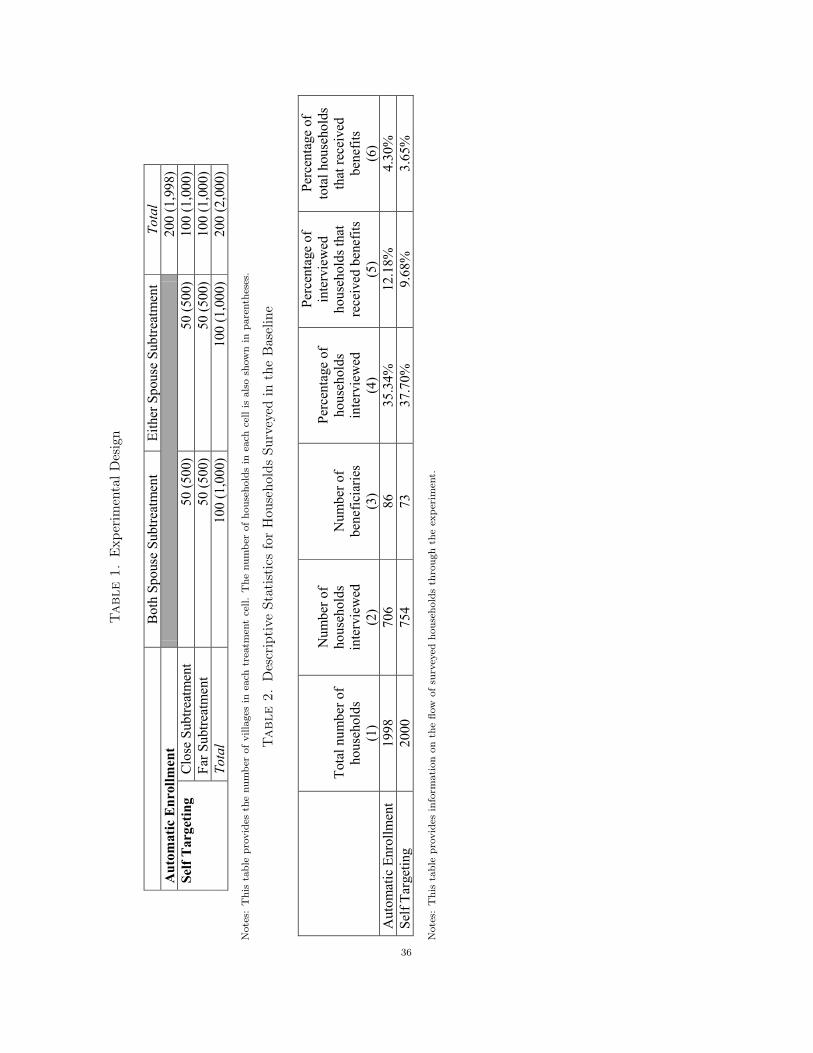
Tabl

e1.

Exp

erim

enta

lDes

ign

B

oth

Spou

se S

ubtre

atm

ent

Eith

er S

pous

e Su

btre

atm

ent

Tota

l A

utom

atic

Enr

ollm

ent

20

0 (1

,998

) Se

lf T

arge

ting

Clo

se S

ubtre

atm

ent

50 (5

00)

50 (5

00)

100

(1,0

00)

Far S

ubtre

atm

ent

50 (5

00)

50 (5

00)

100

(1,0

00)

Tota

l 10

0 (1

,000

) 10

0 (1

,000

) 20

0 (2

,000

)

Not

es:

Thi

sta

ble

prov

ides

the

num

ber

ofvi

llage

sin

each

trea

tmen

tce

ll.T

henu

mbe

rof

hous

ehol

dsin

each

cell

isal

sosh

own

inpa

rent

hese

s.

Tabl

e2.

Des

crip

tive

Stat

isti

csfo

rH

ouse

hold

sSu

rvey

edin

the

Bas

elin

e

Tota

l num

ber o

f ho

useh

olds

(1

)

N

umbe

r of

hous

ehol

ds

inte

rvie

wed

(2

)

N

umbe

r of

bene

ficia

ries

(3)

Pe

rcen

tage

of

hous

ehol

ds

inte

rvie

wed

(4

)

Perc

enta

ge o

f in

terv

iew

ed

hous

ehol

ds th

at

rece

ived

ben

efits

(5

)

Perc

enta

ge o

f to

tal h

ouse

hold

s th

at re

ceiv

ed

bene

fits

(6)

Aut

omat

ic E

nrol

lmen

t 19

98

706

86

35.3

4%

12.1

8%

4.30

%

Self

Targ

etin

g 20

00

754

73

37.7

0%

9.68

%

3.65

%

N

otes

:T

his

tabl

epr

ovid

esin

form

atio

non

the

flow

ofsu

rvey

edho

useh

olds

thro

ugh

the

expe

rim

ent.

36

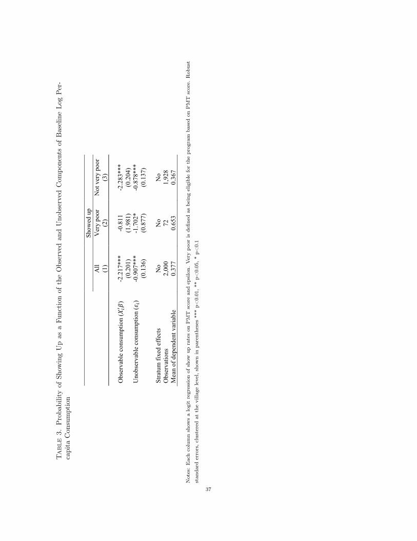
Tabl

e3.

Pro

babi

lity

ofSh

owin

gU

pas

aFu

ncti

onof

the

Obs

erve

dan

dU

nobs

erve

dC

ompo

nent

sof

Bas

elin

eLo

gPe

r-ca

pita

Con

sum

ptio

n

Show

ed u

p

All

Ver

y po

or

Not

ver

y po

or

(1

) (2

) (3

)

O

bser

vabl

e co

nsum

ptio

n (

ᇱ ߚ)

-2.2

17**

* -0

.811

-2

.283

***

(0

.201

) (1

.981

) (0

.204

) U

nobs

erva

ble

cons

umpt

ion

ߝ) )

-0.9

07**

* -1

.702

* -0

.878

***

(0

.136

) (0

.877

) (0

.137

)

St

ratu

m fi

xed

effe

cts

No

No

No

Obs

erva

tions

2,

000

72

1,92

8 M

ean

of d

epen

dent

var

iabl

e 0.

377

0.65

3 0.

367

Not

es:

Eac

hco

lum

nsh

ows

alo

git

regr

essi

onof

show

upra

tes

onP

MT

scor

ean

dep

silo

n.Ver

ypo

oris

defin

edas

bein

gel

igib

lefo

rth

epr

ogra

mba

sed

onP

MT

scor

e.R

obus

tst

anda

rder

rors

,clu

ster

edat

the

villa

gele

vel,

show

nin

pare

nthe

ses

***

p<0.

01,*

*p<

0.05

,*p<

0.1

37

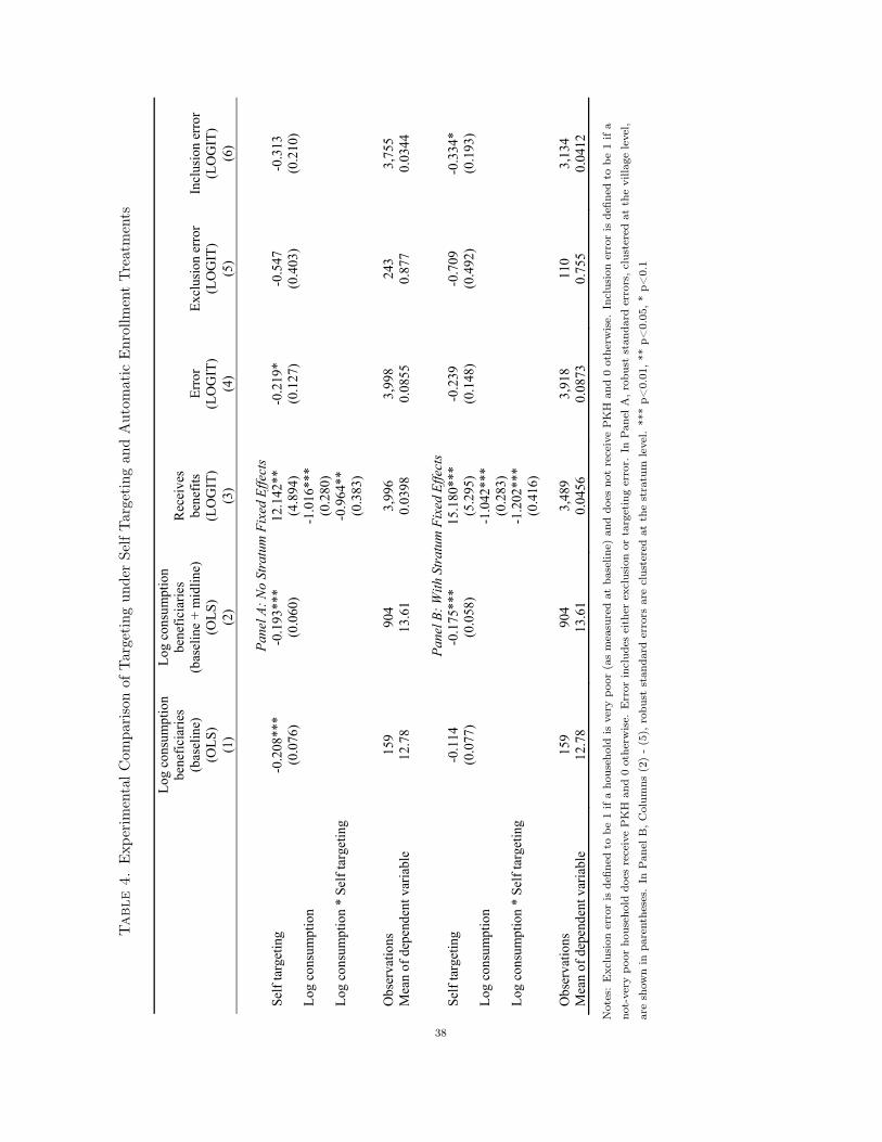
Tabl

e4.

Exp

erim

enta

lCom

pari

son

ofTa

rget

ing

unde

rSe

lfTa

rget

ing

and

Aut

omat

icE

nrol

lmen

tTr

eatm

ents

�Lo

g co

nsum

ptio

n be

nefic

iarie

s (b

asel

ine)

(O

LS)

Log

cons

umpt

ion

bene

ficia

ries

(bas

elin

e +

mid

line)

(O

LS)

Rec

eive

s be

nefit

s (L

OG

IT)

Erro

r (L

OG

IT)

Excl

usio

n er

ror

(LO

GIT

) In

clus

ion

erro

r (L

OG

IT)

�(1

) (2

) (3

) (4

) (5

) (6

)

Pane

l A: N

o St

ratu

m F

ixed

Effe

cts

Self

targ

etin

g -0

.208

***

-0.1

93**

* 12

.142

**

-0.2

19*

-0.5

47

-0.3

13

(0

.076

) (0

.060

) (4

.894

) (0

.127

) (0

.403

) (0

.210

) Lo

g co

nsum

ptio

n

-1

.016

***

(0.2

80)

Lo

g co

nsum

ptio

n *

Self

targ

etin

g

-0

.964

**

(0.3

83)

Obs

erva

tions

15

9 90

4 3,

996

3,99

8 24

3 3,

755

Mea

n of

dep

ende

nt v

aria

ble

12.7

8 13

.61

0.03

98

0.08

55

0.87

7 0.

0344

��

Pane

l B: W

ith S

trat

um F

ixed

Effe

cts

Self

targ

etin

g -0

.114

-0

.175

***

15.1

80**

* -0

.239

-0

.709

-0

.334

*

(0.0

77)

(0.0

58)

(5.2

95)

(0.1

48)

(0.4

92)

(0.1

93)

Log

cons

umpt

ion

-1.0

42**

*

(0

.283

)

Log

cons

umpt

ion

* Se

lf ta

rget

ing

-1.2

02**

*

(0

.416

)

O

bser

vatio

ns

159

904

3,48

9 3,

918

110

3,13

4 M

ean

of d

epen

dent

var

iabl

e 12

.78

13.6

1 0.

0456

0.

0873

0.

755

0.04

12

� ��

Not

es:

Exc

lusi

oner

ror

isde

fined

tobe

1if

aho

useh

old

isve

rypo

or(a

sm

easu

red

atba

selin

e)an

ddo

esno

tre

ceiv

eP

KH

and

0ot

herw

ise.

Incl

usio

ner

ror

isde

fined

tobe

1if

ano

t-ve

rypo

orho

useh

old

does

rece

ive

PK

Han

d0

othe

rwis

e.E

rror

incl

udes

eith

erex

clus

ion

orta

rget

ing

erro

r.In

Pan

elA

,rob

ust

stan

dard

erro

rs,c

lust

ered

atth

evi

llage

leve

l,ar

esh

own

inpa

rent

hese

s.In

Pan

elB

,Col

umns

(2)

-(5

),ro

bust

stan

dard

erro

rsar

ecl

uste

red

atth

est

ratu

mle

vel.

***

p<0.

01,*

*p<

0.05

,*p<

0.1

38

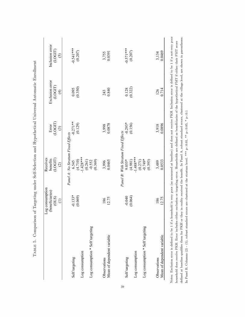
Tabl

e5.

Com

pari

son

ofTa

rget

ing

unde

rSe

lf-Se

lect

ion

and

Hyp

othe

tica

lUni

vers

alA

utom

atic

Enr

ollm

ent

Lo

g co

nsum

ptio

n (b

enef

icia

ries)

(O

LS)

Rec

eive

s be

nefit

s (L

OG

IT)

Erro

r (L

OG

IT)

Excl

usio

n er

ror

(LO

GIT

) In

clus

ion

erro

r (L

OG

IT)

(1

) (2

) (3

) (4

) (5

)

Pane

l A: N

o St

ratu

m F

ixed

Effe

cts

Self

targ

etin

g -0

.133

* 6.

545

-0.2

71**

0.

095

-0.5

41**

*

(0.0

69)

(4.7

10)

(0.1

29)

(0.3

50)

(0.2

07)

Log

cons

umpt

ion

-1

.428

***

(0

.261

)

Log

cons

umpt

ion

* Se

lf ta

rget

ing

-0

.552

(0.3

69)

O

bser

vatio

ns

186

3,99

6 3,

998

24

3

3,75

5 M

ean

of d

epen

dent

var

iabl

e 12

.75

0.04

65

0.08

78

0.84

0 0.

0391

Pane

l B: W

ith S

trat

um F

ixed

Effe

cts

Self

targ

etin

g -0

.040

9.

055*

-0

.293

* 0.

128

-0.5

71**

*

(0.0

64)

(4.9

81)

(0.1

56)

(0.3

22)

(0.2

07)

Log

cons

umpt

ion

-1

.488

***

(0

.271

)

Log

cons

umpt

ion

* Se

lf ta

rget

ing

-0

.749

*

(0.3

93)

O

bser

vatio

ns

186

3,48

9 3,

918

126

3,13

4 M

ean

of d

epen

dent

var

iabl

e 12

.75

0.05

33

0.08

96

0.71

4 0.

0469

Not

es:

Exc

lusi

oner

ror

isde

fined

tobe

1if

aho

useh

old

isve

rypo

or(a

sm

easu

red

atba

selin

e)an

ddo

esno

tre

ceiv

eP

KH

.Inc

lusi

oner

ror

isde

fined

tobe

1if

ano

t-ve

rypo

orho

useh

old

does

rece

ive

PK

H.E

rror

incl

udes

eith

erex

clus

ion

orta

rget

ing

erro

r.H

ouse

hold

sar

ede

fined

asbe

nefic

iari

esof

the

hypo

thet

ical

PM

Tif

eith

erth

eir

PM

Tsc

ore

defin

edat

base

line

qual

ifies

them

for

PK

Hor

they

inre

ality

rece

ived

the

bene

fit.

InPan

elA

,rob

ust

stan

dard

erro

rs,c

lust

ered

atth

evi

llage

leve

l,ar

esh

own

inpa

rent

hese

s.In

Pan

elB

,Col

umns

(2)

-(5

),ro

bust

stan

dard

erro

rsar

ecl

uste

red

atth

est

ratu

mle

vel.

***

p<0.

01,*

*p<

0.05

,*p<

0.1

39

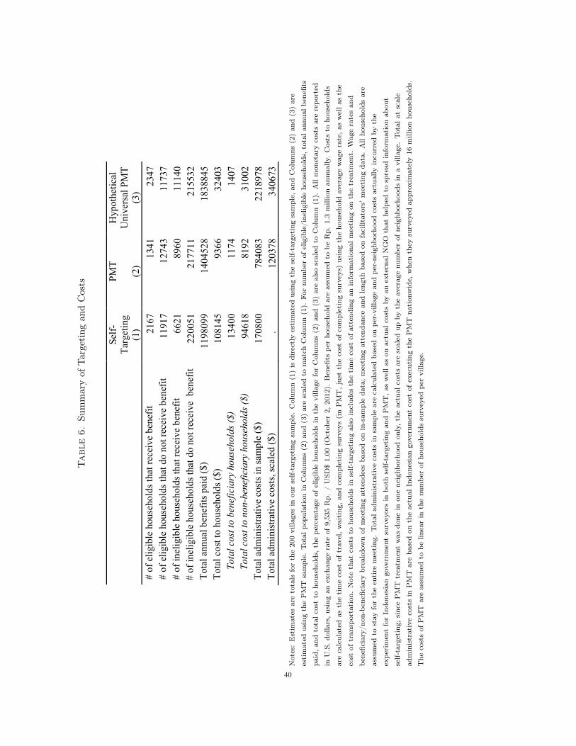
Tabl

e6.

Sum

mar

yof

Targ

etin

gan

dC

osts

Se

lf-Ta

rget

ing

(1)

PMT (2)

Hyp

othe

tical

U

nive

rsal

PM

T (3

) #

of e

ligib

le h

ouse

hold

s tha

t rec

eive

ben

efit

2167

13

41

2347

#

of e

ligib

le h

ouse

hold

s tha

t do

not r

ecei

ve b

enef

it

119

17

1

2743

117

37

# of

inel

igib

le h

ouse

hold

s tha

t rec

eive

ben

efit

6621

89

60

1

1140

#

of in

elig

ible

hou

seho

lds t

hat d

o no

t rec

eive

ben

efit

2

2005

1

217

711

2

1553

2 To

tal a

nnua

l ben

efits

pai

d ($

)

1198

099

14

0452

8

1838

845

Tota

l cos

t to

hous

ehol

ds ($

)

108

145

9366

324

03

T

otal

cos

t to

bene

ficia

ry h

ouse

hold

s ($

)

134

00

1174

14

07

T

otal

cos

t to

non-

bene

ficia

ry h

ouse

hold

s ($

)

946

18

8192

310

02

Tota

l adm

inis

trativ

e co

sts i

n sa

mpl

e ($

)

170

800

7

8408

3

2218

978

Tota

l adm

inis

trativ

e co

sts,

scal

ed ($

)

.

120

378

3

4067

3

Not

es:

Est

imat

esar

eto

tals

for

the

200

villa

ges

inou

rse

lf-ta

rget

ing

sam

ple.

Col

umn

(1)

isdi

rect

lyes

tim

ated

usin

gth

ese

lf-ta

rget

ing

sam

ple,

and

Col

umns

(2)

and

(3)

are

esti

mat

edus

ing

the

PM

Tsa

mpl

e.Tot

alpo

pula

tion

inC

olum

ns(2

)an

d(3

)ar

esc

aled

tom

atch

Col

umn

(1).

For

num

ber

ofel

igib

le/i

nelig

ible

hous

ehol

ds,t

otal

annu

albe

nefit

spa

id,a

ndto

talc

ost

toho

useh

olds

,the

perc

enta

geof

elig

ible

hous

ehol

dsin

the

villa

gefo

rC

olum

ns(2

)an

d(3

)ar

eal

sosc

aled

toC

olum

n(1

).A

llm

onet

ary

cost

sar

ere

port

edin

U.S

.dol

lars

,usi

ngan

exch

ange

rate

of9,

535

Rp.

/U

SD$

1.00

(Oct

ober

2,20

12).

Ben

efits

per

hous

ehol

dar

eas

sum

edto

beR

p.1.

3m

illio

nan

nual

ly.

Cos

tsto

hous

ehol

dsar

eca

lcul

ated

asth

eti

me

cost

oftr

avel

,wai

ting

,and

com

plet

ing

surv

eys

(in

PM

T,j

ust

the

cost

ofco

mpl

etin

gsu

rvey

s)us

ing

the

hous

ehol

dav

erag

ew

age

rate

,as

wel

las

the

cost

oftr

ansp

orta

tion

.N

ote

that

cost

sto

hous

ehol

dsin

self-

targ

etin

gal

soin

clud

esth

eti

me

cost

ofat

tend

ing

anin

form

atio

nalm

eeti

ngon

the

trea

tmen

t.W

age

rate

san

dbe

nefic

iary

/non

-ben

efici

ary

brea

kdow

nof

mee

ting

atte

ndee

sba

sed

onin

-sam

ple

data

;mee

ting

atte

ndan

cean

dle

ngth

base

don

faci

litat

ors’

mee

ting

data

.A

llho

useh

olds

are

assu

med

tost

ayfo

rth

een

tire

mee

ting

.Tot

alad

min

istr

ativ

eco

sts

insa

mpl

ear

eca

lcul

ated

base

don

per-

villa

gean

dpe

r-ne

ighb

orho

odco

sts

actu

ally

incu

rred

byth

eex

peri

men

tfo

rIn

done

sian

gove

rnm

ent

surv

eyor

sin

both

self-

targ

etin

gan

dP

MT

,as

wel

las

onac

tual

cost

sby

anex

tern

alN

GO

that

help

edto

spre

adin

form

atio

nab

out

self-

targ

etin

g;si

nce

PM

Ttr

eatm

ent

was

done

inon

ene

ighb

orho

odon

ly,t

heac

tual

cost

sar

esc

aled

upby

the

aver

age

num

ber

ofne

ighb

orho

ods

ina

villa

ge.

Tot

alat

scal

ead

min

istr

ativ

eco

sts

inP

MT

are

base

don

the

actu

alIn

done

sian

gove

rnm

ent

cost

ofex

ecut

ing

the

PM

Tna

tion

wid

e,w

hen

they

surv

eyed

appr

oxim

atel

y16

mill

ion

hous

ehol

ds.

The

cost

sof

PM

Tar

eas

sum

edto

belin

ear

inth

enu

mbe

rof

hous

ehol

dssu

rvey

edpe

rvi

llage

.

40

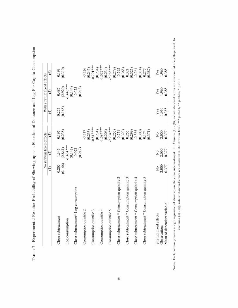
Tabl

e7.

Exp

erim

enta

lRes

ults

:P

roba

bilit

yof

Show

ing

upas

aFu

ncti

onof

Dis

tanc

ean

dLo

gPe

rC

apit

aC

onsu

mpt

ion

N

o st

ratu

m fi

xed

effe

cts

W

ith st

ratu

m fi

xed

effe

cts

(1

) (2

) (3

)

(4)

(5)

(6)

Clo

se su

btre

atm

ent

0.20

5 1.

345

0.19

5

0.27

5 0.

485

0.19

3

(0.1

46)

(2.8

41)

(0.2

38)

(0

.168

) (2

.920

) (0

.310

) Lo

g co

nsum

ptio

n

-1.4

34**

*

-1.4

46**

*

(0.1

43)

(0

.144

)

Clo

se su

btre

atm

ent*

Log

con

sum

ptio

n

-0.0

93

-0

.023

(0.2

17)

(0

.218

)

Con

sum

ptio

n qu

intil

e 2

-0.3

17

-0

.326

(0.2

33)

(0

.245

) C

onsu

mpt

ion

quin

tile

3

-0

.813

***

-0

.791

***

(0

.231

)

(0.2

34)

Con

sum

ptio

n qu

intil

e 4

-1.0

84**

*

-1.0

72**

*

(0.2

06)

(0

.234

) C

onsu

mpt

ion

quin

tile

5

-2

.204

***

-2

.265

***

(0

.257

)

(0.2

79)

Clo

se su

btre

atm

ent *

Con

sum

ptio

n qu

intil

e 2

-0.2

71

-0

.292

(0.3

23)

(0

.368

) C

lose

subt

reat

men

t * C

onsu

mpt

ion

quin

tile

3

0.

255

0.

321

(0

.299

)

(0.3

25)

Clo

se su

btre

atm

ent *

Con

sum

ptio

n qu

intil

e 4

-0.3

85

-0

.261

(0.3

00)

(0

.314

) C

lose

subt

reat

men

t * C

onsu

mpt

ion

quin

tile

5

0.

174

0.

277

(0

.371

)

(0.3

87)

Stra

tum

fixe

d ef

fect

s N

o N

o N

o

Yes

Y

es

Yes

O

bser

vatio

ns

2,00

0 2,

000

2,00

0

1,96

0 1,

960

1,96

0 M

ean

of d

epen

dent

var

iabl

e 0.

377

0.37

7 0.

377

0.

385

0.38

5 0.

385

N

otes

:E

ach

colu

mn

pres

ents

alo

git

regr

essi

onof

show

upon

the

clos

esu

b-tr

eatm

ent.

InC

olum

ns(1

)-

(3),

robu

stst

anda

rder

rors

are

clus

tere

dat

the

villa

gele

vel.

InC

olum

ns(4

)-

(6),

robu

stst

anda

rder

rors

are

clus

tere

dat

the

stra

tum

leve

l.**

*p<

0.01

,**

p<0.

05,*

p<0.

1

41

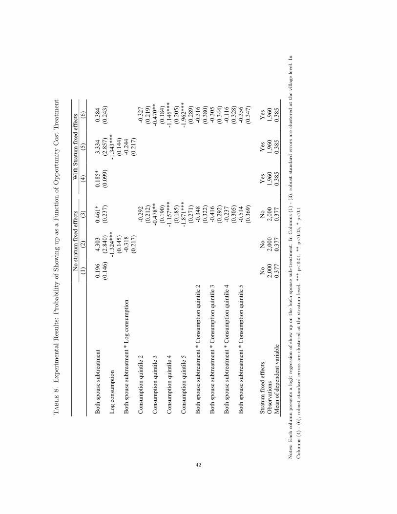
Tabl

e8.

Exp

erim

enta

lRes

ults

:P

roba

bilit

yof

Show

ing

upas

aFu

ncti

onof

Opp

ortu

nity

Cos

tTr

eatm

ent

N

o st

ratu

m fi

xed

effe

cts

W

ith S

tratu

m fi

xed

effe

cts

(1

) (2

) (3

)

(4)

(5)

(6)

Bot

h sp

ouse

subt

reat

men

t 0.

196

4.30

3 0.

461*

0.18

5*

3.33

4 0.

384

(0

.146

) (2

.840

) (0

.237

)

(0.0

99)

(2.8

57)

(0.2

43)

Log

cons

umpt

ion

-1

.324

***

-1

.343

***

(0

.145

)

(0.1

44)

B

oth

spou

se su

btre

atm

ent *

Log

con

sum

ptio

n

-0.3

18

-0

.244

(0.2

17)

(0

.217

)

Con

sum

ptio

n qu

intil

e 2

-0.2

92

-0

.327

(0.2

12)

(0

.219

) C

onsu

mpt

ion

quin

tile

3

-0

.478

**

-0

.470

**

(0

.190

)

(0.1

84)

Con

sum

ptio

n qu

intil

e 4

-1.1

57**

*

-1.1

46**

*

(0.1

85)

(0

.205

) C

onsu

mpt

ion

quin

tile

5

-1

.871

***

-1

.962

***

(0

.271

)

(0.2

89)

Bot

h sp

ouse

subt

reat

men

t * C

onsu

mpt

ion

quin

tile

2

-0

.348

-0.3

16

(0

.322

)

(0.3

80)

Bot

h sp

ouse

subt

reat

men

t * C

onsu

mpt

ion

quin

tile

3

-0

.416

-0.3

05

(0

.292

)

(0.3

44)

Bot

h sp

ouse

subt

reat

men

t * C

onsu

mpt

ion

quin

tile

4

-0

.237

-0.1

16

(0

.305

)

(0.3

28)

Bot

h sp

ouse

subt

reat

men

t * C

onsu

mpt

ion

quin

tile

5

-0

.514

-0.3

56

(0

.369

)

(0.3

47)

Stra

tum

fixe

d ef

fect

s N

o N

o N

o

Yes

Y

es

Yes

O

bser

vatio

ns

2,00

0 2,

000

2,00

0

1,96

0 1,

960

1,96

0 M

ean

of d

epen

dent

var

iabl

e 0.

377

0.37

7 0.

377

0.

385

0.38

5 0.

385

Not

es:

Eac

hco

lum

npr

esen

tsa

logi

tre

gres

sion

ofsh

owup

onth

ebo

thsp

ouse

sub-

trea

tmen

t.In

Col

umns

(1)

-(3

),ro

bust

stan

dard

erro

rsar

ecl

uste

red

atth

evi

llage

leve

l.In

Col

umns

(4)

-(6

),ro

bust

stan

dard

erro

rsar

ecl

uste

red

atth

est

ratu

mle

vel.

***

p<0.

01,*

*p<

0.05

,*p<

0.1

42

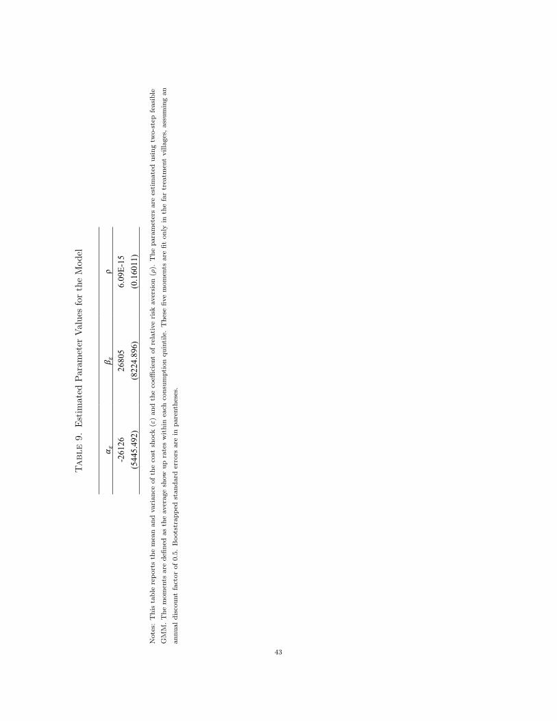
Tabl

e9.

Est

imat

edPa

ram

eter

Val

ues

for

the

Mod

el

ߙ ఌ

ߚ ఌ

ȡ -2

6126

26

805

6.09

E-15

(5

445.

492)

(8

224.

896)

(0

.160

11)

7KLV�WDEOH�UHSRUWV�WKH�PHDQ�DQG�YDULDQFH�RI�WKH�FRVW�VK

RFN����DQG�WKH�

FRHIILFLHQW�RI�UHODWLYH�ULVN�DYHUVLRQ��ȡ���7KH�SDUDPHWHUV�DUH�HVWLPDWHG�

usin

g tw

o-st

ep fe

asib

le G

MM

. The

mom

ents

are

def

ined

as

the

aver

age

show

up ra

tes

with

in e

ach

cons

umpt

ion

quin

tile.

The

se fi

ve m

omen

ts a

re

fit o

nly

in th

e fa

r pop

ulat

ion,

ass

umin

g an

ann

ual d

isco

unt f

acto

r of 0

.5.

Boo

tstra

pped

sta

ndar

d er

rors

are

in p

aren

thes

es.

Not

es:

Thi

sta

ble

repo

rts

the

mea

nan

dva

rian

ceof

the

cost

shoc

k("

)an

dth

eco

effici

ent

ofre

lati

veri

skav

ersi

on(⇢

).T

hepa

ram

eter

sar

ees

tim

ated

usin

gtw

o-st

epfe

asib

leG

MM

.The

mom

ents

are

defin

edas

the

aver

age

show

upra

tes

wit

hin

each

cons

umpt

ion

quin

tile

.T

hese

five

mom

ents

are

fiton

lyin

the

far

trea

tmen

tvi

llage

s,as

sum

ing

anan

nual

disc

ount

fact

orof

0.5.

Boo

tstr

appe

dst

anda

rder

rors

are

inpa

rent

hese

s.

43

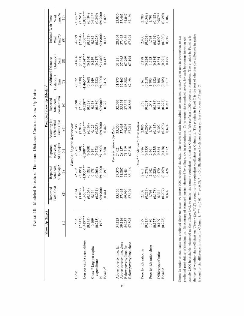
Tabl

e10

.M

odel

edE

ffect

sof

Tim

ean

dD

ista

nce

Cos

tson

Show

Up

Rat

es

Sh

ow U

p (E

xp.)

Pr

edic

ted

Show

Up

(Mod

el)†

R

epor

ted

Tot

al C

ost

Rep

orte

d T

otal

cos

t, SD

[eps

]/2

Rep

orte

d to

tal c

ost,

SD[e

ps]=

0

Ass

umin

g N

o D

iffer

entia

l T

rave

l Cos

t

Rep

orte

d to

tal c

ost,

cons

tant

mu

Add

ition

al D

ista

nce

Infla

ted

Wai

t Tim

e

D

ista

nce

+ 3k

m

Dis

tanc

e +

6km

W

ait

Tim

e*3

Wai

t T

ime*

6

(1)

(2

) (3

) (4

) (5

) (6

) (7

) (8

) (9

) (1

0)

Pa

nel A

: Log

istic

Reg

ress

ions

C

lose

1.

563

-1

.654

-2

.203

-2

.378

-1

.545

-1

.690

-1

.785

-1

.614

-4

.659

-7

.307

**

(2

.813

)

(3.0

19)

(3.3

95)

(3.5

40)

(2.9

19)

(2.3

56)

(3.0

38)

(2.8

33)

(2.9

74)

(3.2

45)

Log

per c

apita

exp

endi

ture

-1

.419

***

-1

.450

***

-1.9

55**

* -2

.208

***

-1.4

42**

* -0

.328

**

-1.4

65**

* -1

.454

***

-1.7

00**

* -1

.927

***

(0

.145

)

(0.1

64)

(0.1

83)

(0.2

00)

(0.1

64)

(0.1

28)

(0.1

68)

(0.1

64)

(0.1

71)

(0.1

94)

Clo

se *

Log

per

cap

ita

-0.1

09

0.

134

0.17

8 0.

191

0.12

5 0.

138

0.14

9 0.

139

0.38

5 0.

611*

*

expe

nditu

re

(0.2

15)

(0

.231

) (0

.261

) (0

.273

) (0

.223

) (0

.180

) (0

.232

) (0

.217

) (0

.228

) (0

.249

) N

19

73

59

1900

0 59

1900

0 59

1900

0 59

1300

0 59

1900

0 59

1300

0 59

1300

0 59

1900

0 59

1900

0 P-

valu

e‡

0.

441

0.39

7 0.

388

0.44

9 0.

379

0.41

5 0.

417

0.11

5 0.

029

Pa

nel B

: Sho

w-U

p Ra

tes

Abo

ve p

over

ty li

ne, f

ar

34.1

23

33

.165

27

.376

24

.021

33

.350

32

.070

31

.875

31

.211

28

.104

23

.036

A

bove

pov

erty

line

, clo

se

39.1

16

37

.465

31

.807

28

.157

37

.463

35

.164

37

.465

37

.465

37

.465

37

.465

B

elow

pov

erty

line

, far

54

.237

69.9

10

71.4

84

71.7

19

69.8

95

37.3

67

68.8

82

67.9

69

67.4

56

64.0

47

Bel

ow p

over

ty li

ne, c

lose

57

.895

67.1

94

68.1

16

67.6

18

67.2

11

36.8

66

67.1

94

67.1

94

67.1

94

67.1

94

Pa

nel C

: Sho

w-U

p Ra

te R

atio

s Po

or to

rich

ratio

, far

1.

589

2.

108

2.61

1 2.

986

2.09

6 1.

165

2.16

1 2.

178

2.40

0 2.

780

(0

.215

)

(0.2

13)

(0.2

78)

(0.3

35)

(0.2

06)

(0.2

01)

(0.2

18)

(0.2

24)

(0.2

61)

(0.3

48)

Poor

to ri

ch ra

tio, c

lose

1.

480

1.

793

2.14

2 2.

401

1.79

4 1.

048

1.79

3 1.

793

1.79

3 1.

793

(0

.177

)

(0.1

78)

(0.2

28)

(0.2

55)

(0.1

85)

(0.1

86)

(0.1

82)

(0.1

84)

(0.1

91)

(0.1

85)

Diff

eren

ce o

f rat

ios

0.10

9

0.31

4 0.

470

0.58

4 0.

302

0.11

7 0.

368

0.38

4 0.

607*

0.

987*

* P-

valu

e (0

.278

)

(0.2

77)

(0.3

59)

(0.4

28)

(0.2

76)

(0.2

73)

(0.2

85)

(0.2

91)

(0.3

30)

(0.3

90)

0.

602

0.42

8 0.

352

0.62

4 0.

985

0.51

7 0.

495

0.24

9 0.

067

N

otes

:In

orde

rto

run

logi

tson

pred

icte

dsh

owup

rate

s,w

ecr

eate

3000

copi

esof

the

data

.T

heco

pies

ofea

chin

divi

dual

are

assi

gned

tosh

owup

orno

tin

prop

orti

onto

his

pred

icte

dpr

obab

ility

ofsh

owin

gup

.B

oots

trap

ped

stan

dard

erro

rs,c

lust

ered

byvi

llage

,are

inpa

rent

hese

s.To

com

pute

the

stan

dard

erro

rs,f

orea

chbo

otst

rap

iter

atio

nw

esa

mpl

e2,

000

hous

ehol

ds,c

lust

ered

atth

evi

llage

leve

l,to

mak

eth

esa

mpl

eeq

uiva

lent

toth

atin

Col

umn

1.W

epe

rfor

m1,

000

boot

stra

pit

erat

ions

.T

hep-

valu

ein

Pan

elA

isth

ete

stof

whe

ther

the

coeffi

cien

ton

[Close⇤LogPCE]is

equa

lto

the

equi

vale

ntco

effici

ent

inC

olum

n1.

The

p-va

lue

inPan

elC

isth

ete

stof

whe

ther

the

diffe

renc

ein

rati

osis

equa

lto

the

diffe

renc

ein

rati

osin

Col

umn

1.**

*p<

0.01

,**

p<0.

05,*

p<0.

1Si

gnifi

canc

ele

vels

not

show

non

first

two

row

sof

Pan

elC

.

44

Figure 1. Probability of Obtaining Benefits vs. Log Per Capita Consumption

0.2

.4.6

Mod

eled

rece

ipt o

f ben

efits

11 12 13 14 15Log per capita expenditure

Notes: This figure shows the predicted probability of receiving the benefit, conditional on applying, from a probitmodel of receiving a benefit as a function of Log PCE. We include urban/rural interacted with district fixed effects

in the probit, since the PMT cutoff for inclusion varies slightly for each urban/rural times district cell. Thesepredicted values are the µ(yi) that we use in the model.

Figure 2. Illustration of Utility Gain with No Errors

gain

0

close

far

y* y** consumption

(a) Gain vs. Consumption for Close andFar Sub-Treatments

applied

1

far close

y* y** income

(b) Targeting Improves as Length of Or-deal Increases

45

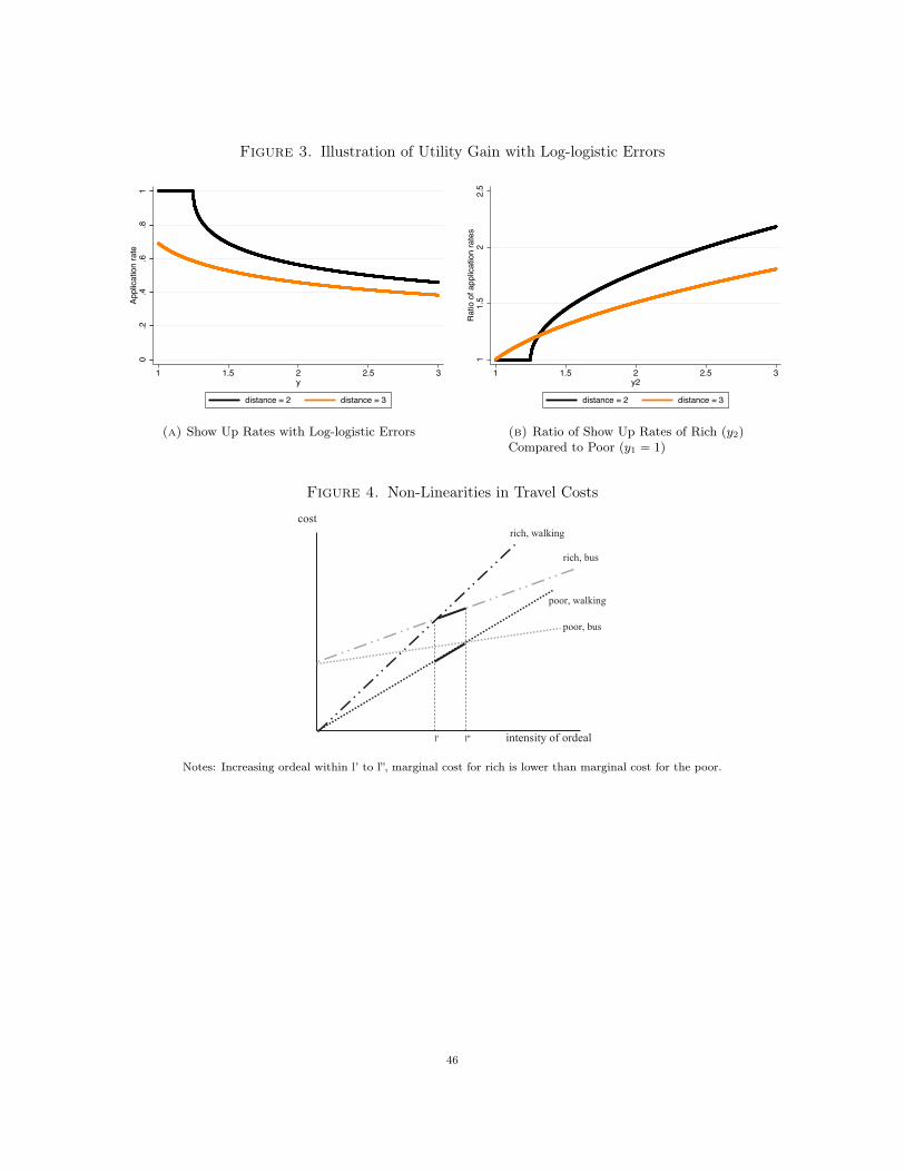
Figure 3. Illustration of Utility Gain with Log-logistic Errors0

.2.4

.6.8

1Ap

plic

atio

n ra

te

1 1.5 2 2.5 3y

distance = 2 distance = 3

(a) Show Up Rates with Log-logistic Errors

11.

52

2.5

Rat

io o

f app

licat

ion

rate

s

1 1.5 2 2.5 3y2

distance = 2 distance = 3

(b) Ratio of Show Up Rates of Rich (y2)Compared to Poor (y1 = 1)

Figure 4. Non-Linearities in Travel Costscost

rich, walking

rich, bus

poor, walking

poor, bus

l' l'' intensity of ordeal

Notes: Increasing ordeal within l’ to l”, marginal cost for rich is lower than marginal cost for the poor.

46

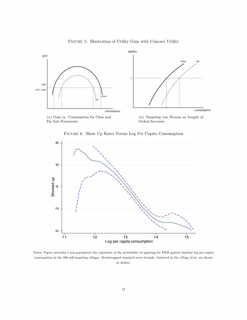
Figure 5. Illustration of Utility Gain with Concave Utility

gain

apply

don’t apply close far

consumption

(a) Gain vs. Consumption for Close andFar Sub-Treatments

applies

close far

1

consumption

(b) Targeting can Worsen as Length ofOrdeal Increases

Figure 6. Show Up Rates Versus Log Per Capita Consumption

0.2

.4.6

.8Sh

owed

up

11 12 13 14 15Log per capita consumption

Notes: Figure provides a non-parametric fan regression of the probability of applying for PKH against baseline log per capitaconsumption in the 200 self-targeting villages. Bootstrapped standard error bounds, clustered at the village level, are shown

in dashes.

47

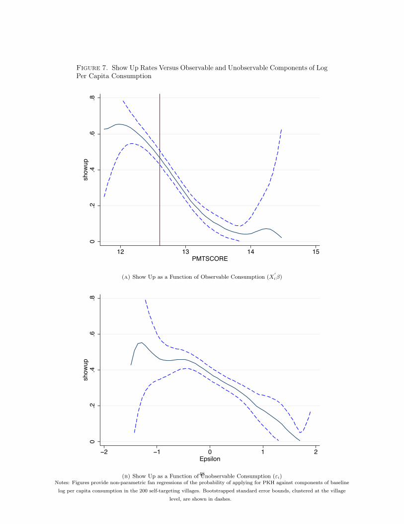
Figure 7. Show Up Rates Versus Observable and Unobservable Components of LogPer Capita Consumption

0.2

.4.6

.8show

up

12 13 14 15PMTSCORE

(a) Show Up as a Function of Observable Consumption (X0i�)

0.2

.4.6

.8show

up

−2 −1 0 1 2Epsilon

(b) Show Up as a Function of Unobservable Consumption ("i)Notes: Figures provide non-parametric fan regressions of the probability of applying for PKH against components of baselinelog per capita consumption in the 200 self-targeting villages. Bootstrapped standard error bounds, clustered at the village

level, are shown in dashes.

48

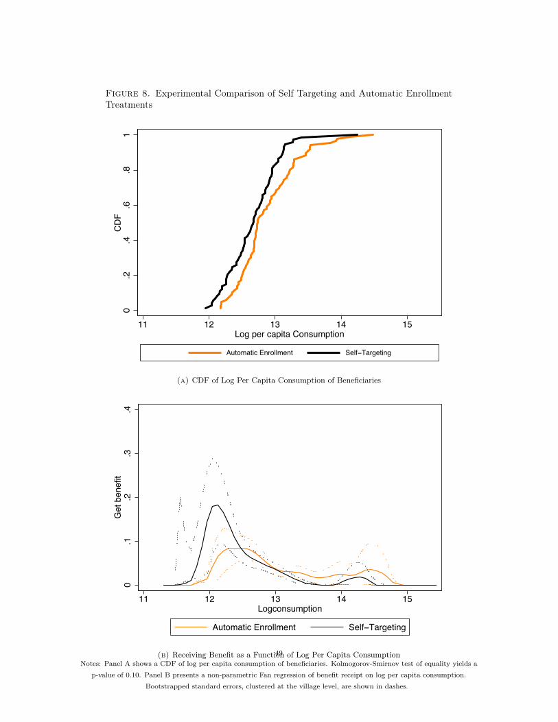
Figure 8. Experimental Comparison of Self Targeting and Automatic EnrollmentTreatments

0.2

.4.6

.81

CD

F

11 12 13 14 15Log per capita Consumption

Automatic Enrollment Self−Targeting

(a) CDF of Log Per Capita Consumption of Beneficiaries

0.1

.2.3

.4G

et b

enef

it

11 12 13 14 15Logconsumption

Automatic Enrollment Self−Targeting

(b) Receiving Benefit as a Function of Log Per Capita ConsumptionNotes: Panel A shows a CDF of log per capita consumption of beneficiaries. Kolmogorov-Smirnov test of equality yields a

p-value of 0.10. Panel B presents a non-parametric Fan regression of benefit receipt on log per capita consumption.Bootstrapped standard errors, clustered at the village level, are shown in dashes.

49

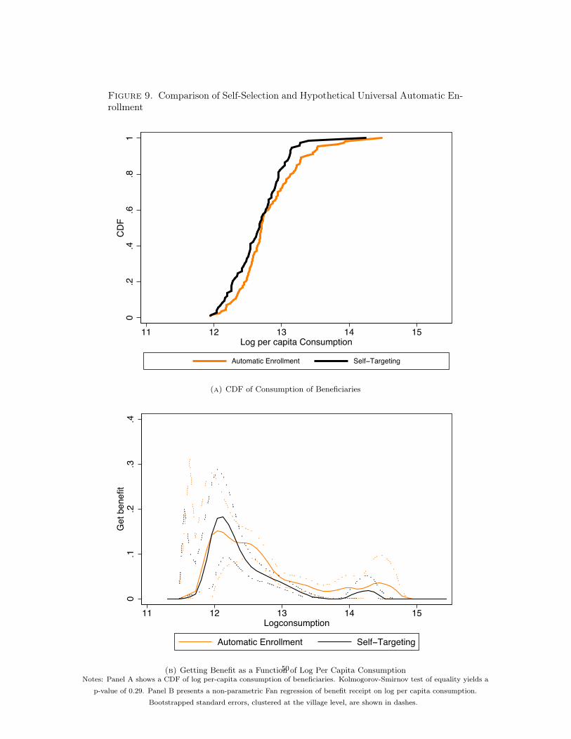
Figure 9. Comparison of Self-Selection and Hypothetical Universal Automatic En-rollment

0.2

.4.6

.81

CD

F

11 12 13 14 15Log per capita Consumption

Automatic Enrollment Self−Targeting

(a) CDF of Consumption of Beneficiaries

0.1

.2.3

.4G

et b

enef

it

11 12 13 14 15Logconsumption

Automatic Enrollment Self−Targeting

(b) Getting Benefit as a Function of Log Per Capita ConsumptionNotes: Panel A shows a CDF of log per-capita consumption of beneficiaries. Kolmogorov-Smirnov test of equality yields a

p-value of 0.29. Panel B presents a non-parametric Fan regression of benefit receipt on log per capita consumption.Bootstrapped standard errors, clustered at the village level, are shown in dashes.

50

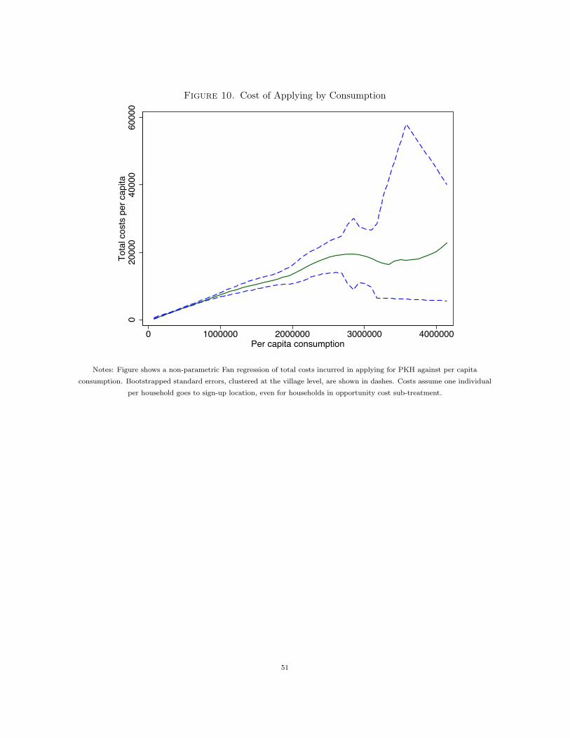
Figure 10. Cost of Applying by Consumption

020

000

4000

060

000

Tota

l cos

ts p

er c

apita

0 1000000 2000000 3000000 4000000Per capita consumption

Notes: Figure shows a non-parametric Fan regression of total costs incurred in applying for PKH against per capitaconsumption. Bootstrapped standard errors, clustered at the village level, are shown in dashes. Costs assume one individual

per household goes to sign-up location, even for households in opportunity cost sub-treatment.

51

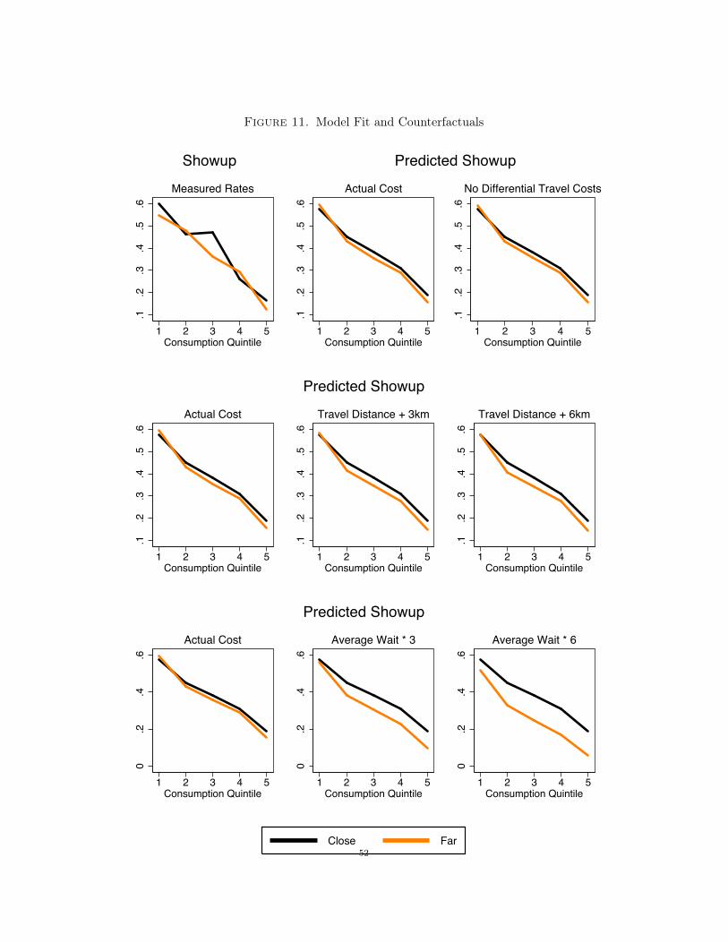
Figure 11. Model Fit and Counterfactuals.1

.2.3

.4.5

.6

1 2 3 4 5Consumption Quintile

Measured Rates

.1.2

.3.4

.5.6

1 2 3 4 5Consumption Quintile

Actual Cost

.1.2

.3.4

.5.6

1 2 3 4 5Consumption Quintile

No Differential Travel Costs

Showup Predicted Showup .1

.2.3

.4.5

.6

1 2 3 4 5Consumption Quintile

Actual Cost

.1.2

.3.4

.5.6

1 2 3 4 5Consumption Quintile

Travel Distance + 3km

.1.2

.3.4

.5.6

1 2 3 4 5Consumption Quintile

Travel Distance + 6km

Predicted Showup

0.2

.4.6

1 2 3 4 5Consumption Quintile

Actual Cost

0.2

.4.6

1 2 3 4 5Consumption Quintile

Average Wait * 3

0.2

.4.6

1 2 3 4 5Consumption Quintile

Average Wait * 6

Predicted Showup

Close Far52