SELECTION BIAS, DEMOGRAPHIC EFFECTS AND ABILITY EFFECTS IN COMMON VALUE AUCTION EXPERIMENTS

Marco Casari Purdue University

John C. Ham

University of Southern California, the Federal Reserve Bank of San Francisco and IZA

John H. Kagel*

Ohio State University

8/11/2006

Abstract

Inexperienced women, along with economics and business majors, are much more susceptible to the winner’s curse, as are subjects with lower SAT/ACT scores. There are strong selection effects in bid function estimates for inexperienced and experienced subjects due to bankruptcies and bidders who have lower earnings returning less frequently as experienced subjects. These selection effects are not identified using standard econometric techniques but are identified through experimental treatment effects. Ignoring these selection effects leads to misleading estimates of learning. JEL classification: C9, D44, C24, J16. Key words: common value auction experiments, selection effects, econometric methods, gender and ability effects, learning.

* Casari, Krannert School of Management, Purdue University, 403 W. State St., West Lafayette, IN 47907(e-mail: casari@purdue.edu): Ham, Department of Economics, University of Southern California, Kaprielian Hall (KAP) 300,Los Angeles, CA 90089, (e-mail: johnham@usc.edu): Kagel, Department of Economics, Ohio State University, 410 Arps Hall, 1945 North High Street, Columbus, OH 43210-1172, (e-mail: kagel.4@osu.edu). Earlier versions of this paper were presented at the Meetings of the Econometric Society, Washington D. C., at the Simposio de Analisi Economico in Seville, Spain, at a Conference on Experiments and Econometrics at New York University, at the 11th Annual Panel Data Conference, at the 2004 SITE conference, and at seminars at the University of Alicante, Bilkent University, Claremont McKenna College, Columbia University, Ohio State University, Purdue University, UCLA, University of Torino, and University of Siena. We thank Linda Babcock, Rachel Croson, John Duffy, Dan Levin, John List, Geert Ridder, Jeffrey Smith, Lise Vesterlund, Simon Wilkie and participants at meetings and seminars for valuable comments, as well as four anonymous referees. We thank Serkan Ozbeklik and Alex Brown for excellent research assistance, Robert Vandyne, Jr. from Student Enrollment and Research Services at the Ohio State University for his help in obtaining detailed demographic and ability data on students, and Jo Ducey for editorial and administrative assistance. Some of this research was conducted while Ham was a visitor at the Federal Reserve Bank of New York and Casari was a visitor at CODE in Barcelona under a Marie Curie fellowship where they were provided hospitable and productive environments. This research has been supported by National Science Foundation Grant (SES-0136928). Any opinions, findings, and conclusions or recommendations in this material are those of the authors and do not necessarily reflect the views of the National Science Foundation, the European Commission, the Federal Reserve Bank of New York, the Federal Reserve Bank of San Francisco or the Federal Reserve System. We are responsible for any errors.

1

Common value auctions have been an active area of research in the economics literature.

Initial results from Outer Continental Shelf (OCS) oil lease auctions (often considered the

canonical example of a common value auction) suggested that bidders suffered from a winner’s

curse – winning bidders systematically overbidding and losing money as a consequence (E. C.

Capen, R. V. Clapp and W. M. Campbell, 1971). Experiments designed to investigate this claim

have shown that inexperienced bidders consistently fall prey to the winner’s curse, bidding above

the expected value conditional on winning and earning negative average profits as a

consequence. It is only with experience that bidders learn to avoid the worst effects of the

winner’s curse and earn a respectable share of the profits predicted under the risk neutral Nash

equilibrium (see John H. Kagel and Dan Levin, 2002, for a review of the experimental

literature). The transition from inexperienced bidders suffering persistent losses to experienced

bidders earning respectable profits is characterized by large numbers of bidders going bankrupt,

with these bankrupt bidders much less likely to return as experienced subjects.1

These results raise a number of substantive questions regarding bidding behavior in

common value auctions. First, the winner’s curse involves a type of judgmental error – bidders’

failure to account for the adverse selection effect conditional on winning. As such it joins a

burgeoning economics literature indicating that bounded cognitive abilities can explain many

observed empirical deviations from full rationality. To investigate this issue we study the effects

of Scholastic Aptitude and American College Test (SAT/ACT) scores and grade point average

on subjects’ ability to avoid the winner’s curse, along with subjects’ major and gender. Ours is

one of the first studies to include SAT/ACT scores to control for ability effects in the

experimental economics literature.2

The second motivation for the present paper is to better understand the process whereby

experienced bidders “learn” to avoid the winner’s curse. Bidders learn to avoid the winner’s

curse in one of two (not mutually exclusive) ways: Less able bidders may simply go bankrupt,

exit the market and not return for subsequent experimental sessions – a market selection effect.

Alternatively, individual bidders may learn to adjust their bidding so as to avoid the winner’s 1 Claims of a winner’s curse in field settings have been subject to considerable dispute, representing as they do out of equilibrium play. Robert Wilson (1992) reviews the literature with respect to OCS auctions concluding that there is considerable evidence consistent with a winner’s curse in early OCS auctions. 2 See also Daniel J. Benjamin and Jesse M. Shapiro (2005) who use self reported SAT/ACT scores. Note that we use SAT/ACT scores provided by the university, while self-reported (recall) scores are likely to be subject to considerable measurement error. An alternative, closely related, approach is to employ cognitive tests directly related to the question at hand (e.g., Gary Charness and Levin, 2005, and Shane Frederick, 2005).

2

curse. In addition to being of inherent interest, distinguishing between these alternative

adjustment processes affects the kinds of learning models one needs to develop to characterize

the evolution of behavior over time in common value auctions. It also has potential public policy

implications, as legislation on corporate bankruptcy and on procurement contracts is sometimes

directly related to these issues. For example, in all European Union countries competition for

government procurement contracts has been regulated with the explicit goal of fostering the

acquisition of expertise and to minimize the chances of contractors’ bankruptcies (CEE Directive

n. 37, June 13, 1993). One rationale for these rules is the belief that “market selection”, if left

unchecked, operates to the detriment of social welfare maximization in some contexts and does

not leave time for “individual learning” to take place.

Past studies do not typically distinguish between these different sources of learning.

Evidence of individual learning on the part of experienced bidders can be overstated as it may

simply reflect more able bidders, who earn more money as inexperienced subjects, being more

likely to return as experienced subjects. Further, high bankruptcy rates for inexperienced bidders

may severely bias estimates of learning on the part of inexperienced bidders, with the extent and

nature of the bias unexplored to date.

To study learning we have subjects participate in two sessions approximately one week

apart (“week 1” and “week 2”). Learning can take place: (i) during the first session; (ii) between

the two sessions as subjects reflect on their decisions and (iii) during the second session. We

employ a variety of techniques to address selection issues both within weeks and between weeks.

Within a session there may be a selection bias resulting from bankruptcies. To address it we

randomly assigned different initial cash balances to subjects, and induced random shocks to these

balances within the experiment. These manipulations also enable us to identify any potential cash

balance effects on bidding. Between week 1 and week 2 sessions there may be a selection bias

because only a subset of subjects returns for week 2. To address this we provided differential

incentives for returning in week 2.3 That is, we introduced into the experimental design

instruments that could potentially help to identify selection effects using relatively sophisticated

estimators borrowed from the applied econometrics literature (James J. Heckman, 1979,

3 We are treating the individuals who begin the experiment as the population of interest. However, we also compare our sample to the university population they were drawn from. One could worry about differences between student subjects and bidders in field settings. There are a number of studies that examine this issue; see for example Douglas Dyer, Kagel and Levin (1989), Glenn W. Harrison and John A. List (2003) and Steffen Anderson et al. (2005).

3

Keunkwan Ryu, 2001) and that, alternatively, would allow us to obtain unbiased estimates of the

bid equation by simply distinguishing between appropriate sub-samples of our data.

We obtain a number of substantive as well as methodological insights in answering these

questions. First, not surprisingly, ability as measured by SAT/ACT scores matters in terms of

avoiding the winner’s curse. However, the nature of these ability effects are different from what

one might expect as (i) we find more instances of a statistically significant role for composite

SAT/ACT scores than for either math or verbal scores alone and (ii) the biggest and most

consistent impact of ability comes as a result of those with below median scores being more

susceptible to the winner’s curse, as opposed to those with very high scores doing exceptionally

well. The latter continues to be observed for experienced bidders, so that bidders with below

median composite SAT/ACT scores, on average, suffer from a winner’s curse even as

experienced bidders.

Second, we find clear demographic effects as women are much more susceptible to the

winner’s curse as inexperienced bidders than men, although this difference disappears for

experienced bidders. This finding of a gender effect is the more remarkable because it is obtained

while controlling for obvious confounding factors such as ability and college major, factors that

are not typically controlled for in investigating gender effects in experimental economics. In

addition, economics and business majors are much more susceptible to the winner’s curse than

other majors, and continue to do worse even as experienced bidders.

In terms of learning, we find that inexperienced subjects are capable of substantial

individual learning, even those subjects who start out being most susceptible to the winner’s

curse. These results suggest that previous studies are likely to have substantially underestimated

the amount of individual learning that inexperienced bidders are capable of within a session.

This point is most clear when estimating learning in women, who in week 1 start bidding rather

poorly. If endowed with sufficient cash they do catch up to, and do as well as men by the end of

the week 1 session. Further, we find that more able bidders are more likely to return as

experienced subjects, with this factor dominating learning between week 1 and week 2. As such

previous studies are likely to have substantially overestimated the amount of individual subject

learning that occurs when moving from inexperienced to experienced bidders. Finally, we find

some, albeit much smaller than in week 1, learning within week 2 for individual bidders in our

unbiased sample, while finding essentially no learning on the part of experienced bidders in the

4

biased sample. Selection biases within a session are unlikely to be widespread in experimental

economics, as there are few other experimental designs in which bidders go bankrupt.4

However, the selection effects identified between sessions may be present in the many studies

that employ experienced subjects, as basic economic theory leads one to expect that those

subjects who earn more money in an experiment are more likely to return as experienced

subjects. Fortunately the modification we make to the experimental design is able to fully

eliminate the selection problem of who returns in week 2.

In answering these questions we also obtain a number of methodological insights. First,

standard econometric estimators for dealing with selection effects in field data do not identify

any kind of selection effects in our data, in spite of having a relatively large sample by

experimental standards and well identified econometric models. However, the different

experimental treatments built into the experimental design serve to identify, measure, and verify

such effects. In retrospect, these results are not surprising. At least as far back as Ronald A.

Fisher (1935) statisticians have understood that experimental design (through randomization, for

example) could permit the identification of casual effects. On the other hand, econometric

sample selection techniques were designed for large sample situations where randomization is

not possible. These techniques may fail if sample sizes are too small or economic models are

misspecified. Indeed, since Robert J. LaLonde (1986) there has been considerable skepticism

about the ability of these techniques to fully address selection bias, and there has been a move

towards randomization via social and field experiments.

The paper proceeds as follows. Section I specifies the risk neutral Nash equilibrium

(RNNE) bid function for the experimental design, along with some measures of when subjects

have fallen prey to the winner’s curse. Section II outlines the experimental procedures and

provides some general descriptive statistics concerning changes in bidding between weeks 1 and

2, and the potential selection effects present in the data. Section III describes our ability and

demographic measures. Section IV looks at the effect of these demographic and ability measures

on the conditional probability of bankruptcy in each period among inexperienced bidders.

Section V discusses selection effects, and demographic and ability effects, for inexperienced

(week 1) bidders. Section VI addresses the question of selection effects, as well as ability and

4 Of course, any time subjects are exposed to potential losses there is a threat of bankruptcy and selection effects of this sort, so that bankruptcies do occur in other environments; e.g., asset markets (Peter Bossaerts and Charles R. Plott, 2004).

5

demographic effects, for experienced bidders. Section VII discusses the gender effect identified

and relates it to the existing literature on gender effects in economic experiments. The

concluding section of the paper summarizes our main results.

I. Theoretical Considerations: First-Price Sealed-Bid Auctions

In a first-price sealed-bid auction, n bidders compete for a single item. The value of the

item, xo is the same for all bidders (common value) but unknown to them. The value xo was

chosen randomly from a uniform distribution with support [$50, $950]. What each bidder i

knows prior to bidding is a private information signal, ix , drawn independently from a uniform

distribution with support [xo - $15, xo + $15].

For risk neutral bidders the symmetric risk neutral Nash equilibrium (RNNE) bid

function ( )ixγ is given by5

( ) 15 ( )i i ix x h xγ = − + where (1)

( ) [(30 /( 1)]exp[ ( / 30)( 65)]i ih x n n x= + − − , (2)

Equation (1) is the RNNE bid for a bidder with a signal in the interval 65 935ix≤ ≤ . In this

paper we restrict our attention to this interval (called region 2), where the bulk of the

observations lie. The term ( )ih x is positive but quickly becomes negligible as ix increases

beyond 65. Thus for simplicity we ignore it in the discussion that follows, although we do

include it in all relevant regressions.

In common-value auctions bidders usually win the item when they have the highest (or

one of the highest) signals. Let 1n[ |X=x ]iE x be the expected value of the signal conditional on it

being the highest among the n signal values drawn. We define three benchmarks against which to

evaluate bidding: (a) bid your signal; (b) the loss-free bid, and (c) the break-even bid. For signals

in region 2

1n 0[ |X=x ] [( 1) /( 1)]15iE x x n n= + − + . (3)

So that if individuals naively bid their signal, they will overbid and can expect to lose money.

The loss-free bid strategy with the highest probability of winning is to bid ix - 15. The last,

important, benchmark is the break-even bid strategy

5 Derivation of the RNNE bid function, as well as its characterization outside of region 2 can be found in Kagel and Levin (1986) and Kagel and Jean-Francois Richard (2001).

6

( ) [( 1) /( 1)]15i ix x n nγ = − − + , (4)

which yields zero expected profits and will periodically generate losses. When the high signal

holder always wins the item, any bid above ( )ixγ yields an expected loss. For this reason, we

label such bids as falling prey to the “winner’s curse.”

We will compare between the benchmark strategies based on the bid factor, x – γ(x). For

n=6 the bid factor for the RNNE is approximately $15, close to the loss-free strategy. The bid

factor for the break-even strategy is $10.71, about 71% of the RNNE bid factor implied by

equation (1).

The RNNE is based on the assumption of risk neutral bidders, all of whom employ the

same bid function and fully account for the adverse selection effect conditional on winning the

item. The empirical analysis shows that the homogeneity assumption is not tenable as

demographic characteristics and “ability” impact on bidding, and there is some residual,

unexplained, heterogeneity in bidding, as evidenced by a statistically significant subject effect

error term in the regressions. These deviations from the assumptions underlying the theory raise

questions regarding the empirical relevance of benchmarks (a) – (c). They are, however, still

relevant as: (i) Virtually all subjects are bidding above, rather than below, 15ix − in region 2,

and the best response to such rivals is to bid 15ix − (Kagel and Richard, 2001); (ii) Within region

2, regardless of what other explanatory variables are included in the empirically specified bid

function, the coefficient value for own signal value, ix , is indistinguishable from 1.0; (iii)

Bidding above (4) yields negative expected profits both with strict homogeneity in bidding and

in cases where all of one’s rivals are bidding above (4), regardless of the heterogeneity in bid

patterns. As such, for inexperienced bidders at least, (4) still provides a reasonable measure for

whether individual bidders fall prey to the winner’s curse; (iv) Although the impact of risk

aversion on bids in first-price private-value auctions is unambiguous (bidding above the RNNE),

it does not necessarily have the same impact in common-value auctions since bidding above

15ix − creates the possibility of losses. What we can say about risk aversion is that (i) a risk

averse bidder clearly does not want to bid above (4) since to do so yields negative expected

profits and (ii) from an empirical perspective any deviation from risk neutrality will result in an

7

intercept for the bid functions estimated (6a and b below) that is greater than $15 but below [(n-

1)/(n+1)]15.6

To summarize, this section as well as the following empirical sections restrict attention to

bidders with signals in the interval 65 935x≤ ≤ . To avoid the winner’s curse an individual must

bid less than the break-even bid of equation (4). The break-even bid is closer to the RNNE bid of

equation (1), which yields an expected gain, than to their signal (xi), which yields an expected

loss. Because of the risk of losses, bidding above (4) cannot be attributed to risk aversion.

II. Experimental Procedures and Basic Descriptive Statistics

Each experimental session consisted of a series of auctions for a single item of value xo.

All of the information about the underlying distribution of xo and signal values was included in

the instructions. At the end of each auction all bids were posted from highest to lowest along

with the corresponding signal values (bidder identification numbers were suppressed) and the

value of xo. Profits (or losses) were calculated for the high bidder and reported to all bidders.

Each experimental session began with two markets with six bidders each. Assignments

to each market varied randomly between auction periods. To hold the number of bidders, n,

constant in the face of potential bankruptcies, extra bidders were recruited for each session, with

bidders randomly rotated in and out of active bidding between auctions.

We employed three different treatments designed to help identify selection effects:

Control treatment: This treatment matches the standard experimental practice for common-value

auctions, with all subjects given starting capital balances of $10 and a flat show-up fee of $5.

All subjects participating in week 1 were invited back for week 2 where all subjects were again

given starting capital balances of $10 and a flat show-up fee of $5.

Bonus treatment: Starting cash balances were either $10 or $15, with half the subjects randomly

assigned to each cash balance level. Further, following each auction, active bidders were

automatically enrolled in a lottery with a 50% chance of earning $0 or $0.50 in order to provide

additional exogenous variation in cash balances. In addition, a show-up fee of $20 was paid only

after completing week 2’s session, with 50% of week 1 earnings held in escrow as well.7

6 Precise predictions regarding risk aversion exist for second-price and English clock auctions; namely risk averse subjects will bid below the RNNE benchmark. This is not observed for either inexperienced or experienced bidders even in the English clock auctions (Levin, Kagel, and Richard, 1996). 7 Olivier Armantier (2004) employs these procedures to induce subjects to return between sessions in a common value auction experiment aimed at determining the role of information feedback on learning.

8

Random treatment: This was the same as the bonus treatment with the exception that (i) bidders

were given a $5 show-up fee in week 1 along with all of week 1’s earnings and (ii) when inviting

bidders back for week 2, half the subjects (determined randomly) were assigned a show-up fee of

$5, with the other half assigned a show-up fee of $15. Thus, the only difference between this and

the bonus treatment was the incentive for returning in week 2.

Each inexperienced (week 1) session began with two dry runs, followed by thirty

auctions played for cash. Earnings from the auctions, and lottery earnings, were added to starting

cash balances. Once a bidder’s cash balance was non-positive they were declared bankrupt and

no longer permitted to bid.8 Experienced subject sessions employed an abbreviated set of

instructions, a single dry run, and thirty-six auctions played for cash.

Subjects were recruited by e-mail from the general student population at Ohio State

University. Just under 93% were undergraduate students, with the remainder either graduate

students or of unknown status.

Table 1 shows the number of sessions and subjects (listed in parentheses) in each

treatment in weeks 1 and 2. Table 1 also reports some basic descriptive statistics. Three key

factors stand out from the descriptive statistics reported in Table 1. First, there is strong

improvement in performance going from week 1 to week 2, with average profits per auction

going from -$2.47 (large average losses in week 1) to $0.75 (small average profits in week 2),

while average predicted profits remain unchanged between weeks. This conclusion is confirmed

and reinforced by the winner’s curse measure (b > ( )ixγ ), as the frequency of the winner’s curse

drops dramatically both for all bidders and for high bidders. Second, there is severe potential

selection bias within week 1 across all treatments, given the large number of bankruptcies

reported within week 1. Third, there is relatively strong selection bias between weeks 1 and 2 for

the control group and the random group, with 40.0% and 25.9% of week 1 subjects not returning

for week 2 for these two groups, respectively, versus 4% for the bonus group.

8 Because of limited-liability for losses, once cash balances drop below a certain level it is rational, in terms of a one-shot game, to bid modestly above the RNNE assuming that all other bidders employ the RNNE (see, Kagel and Richard, 2001 for estimates of the size of these overbids).

9

III. Demographic and Ability Measures

The consent form gave us permission to collect demographic data from the University

Enrollment Office. It called for providing information regarding gender, SAT and ACT scores,

major, and class standing (freshman, sophomore, etc.).9

The demographic and ability measures employed in the data analysis are as follows:

Gender: Male/Female.

College major: Three categories were established - business and economics, science and

engineering, and a residual category accounting for all other majors.

SAT/ACT scores: These scores result from standardized tests that most high school graduates

take when seeking admission to a US college. A set of binary variables was constructed for three

ability levels - high, median, and low - based on both the SAT and ACT scores.10 The cut-off

points chosen were below the median, between the median and the 95-percentile, and the 95-

percentile or higher. Binary variables were generated for several reasons. First, ACT and SAT

scores are not additive measures of ability but rather rank order measures so that binary scores

are more appropriate than raw scores. Second, this specification is a simple way to capture

possible non-linear impacts of different ability levels. Third, a number of students were missing

SAT or ACT scores (39.4% SAT and 25.5% ACT), which would have increased the fraction of

observations with missing values. Using both scores this way reduces the number of subjects

with a missing value to 13.7% of the sample. Bidders were coded according to their verbal,

mathematical, and combined skills. Although the categories used for SAT/ACT scores are

somewhat arbitrary, they do provide reasonable measures of high, medium and low ability that

we believe are interesting, and the results are robust to small differences in the cut points.

We also explored a number of empirical specifications using grade point average (GPA)

in place of, or in conjunction with, SAT/ACT scores. GPA proved to be a far inferior ability

measure compared to SAT/ACT scores, rarely achieving statistical significance in any of our

specifications. We suspect there are two primary reasons for this. First, we have a number of

freshmen and sophomores in our sample for which GPA would be a very incomplete measure of 9 We do not have information on race since we did not ask for this information on the release. About 15% of the students enrolled at the Ohio State University main campus are classified as minorities: 7.1% African American, 5.2% Asian American, and 2.3% Hispanic, so that this subject population is a poor choice for studying racial differences. We did not obtain information on the economic background of the subjects as this information is not readily available from the university and self-reported information on this score is likely to be quite inaccurate. 10 For a description see http://en.wikipedia.org/wiki/ACT_%28examination%29 and http://en.wikipedia.org/wiki/SAT

10

academic performance. Second, there is likely to be a good deal of heterogeneity in grade scales

both between colleges and between majors within colleges.

Table 2 gives the sample composition according to these demographic and ability

variables for inexperienced bidders, along with the relevant data for the university population

from which the sample was drawn. Men comprise 59.7% of the sample, with the breakdown by

major being 30.2% economics/business majors, 23.4% engineering and science majors, and

46.4% all other majors. There are more men in the sample than in the university population, as

well as a much larger percentage of economics and business majors than the university

population (30.2% versus 12.3%). The latter is to be expected given that we recruited from e-

mail lists for students enrolled in economics classes. Some 20.2% of the sample are in the top

5% (of the national average) with respect to composite SAT/ACT scores (versus 4.9% for the

university), with less than 8.9% scoring below the median (versus 20.9 for the university), and

13.3% not having any SAT/ACT scores (versus 21.1% for the university). The latter are

primarily transfers from regional campuses as these students are not required to take these tests

when transferring to the main campus. They are likely to have lower SAT/ACT scores if we had

their test records, as a number of these regional campus transfers were ineligible to enter to main

campus when they originally applied to college. Thus, our sample population includes students

with significantly higher ability than the university population as measured by the percentage of

students scoring in the top 5% on composite SAT/ACT scores and below median SAT/ACT

scores. This cannot be attributed simply to better non-economics and business students signing

up for economics classes, as we see similar differences in ability between our sample and the

university population for economics and business majors within the sample (see Table A1 in the

online Appendix). Freshmen and sophomores comprise 55.5% of the sample versus 48.2% of the

university population.

When demographic variables are included in the regressions, the reference bidder is a

male subject with an “other” major with SAT/ACT scores between the median and the 95th-

percentile. Our analysis focuses on composite SAT/ACT scores. Results employing verbal and

mathematics SAT/ACT scores in place of the composite score are reported in an online

Appendix but will be referred to in the text.

11

IV. A Duration Model of Bankruptcy

The question to be addressed here is what are the factors behind the large number of

bankruptcies for inexperienced bidders (week 1) reported in Table 1? In particular, are there any

demographic or ability factors that we would otherwise be unaware of behind the bankruptcies?

A natural format for modeling bankruptcies is a hazard, or duration model, since once a subject

goes bankrupt within a given experimental session they are no longer permitted to bid in that

session.

We assume that the probability that a person goes bankrupt in period t , conditional on

not having gone bankrupt in the previous 1t − periods, is given by the discrete-time (logit)

hazard function

( ) ( ), ; , 1/ 1 exp{ }i i it itt Z yλ θ δ γ = + − (5a)

where

1ln( ) .

Kk

it it k ik

y Z tδ γ θ=

= + +∑ (5b)

In (5b) itZ is a vector of explanatory variables and t measures the number of auctions the

individual has actively participated in (including the current one). We are particularly interested

in the coefficient vector δ since itZ includes all of our demographic and ability variables. itZ

also consists of a number of control variables, all of which are determined in the experiment and

are out of the subjects’ control. These include the variable lagcumcash, defined as subjects’

starting cash balance plus any lottery earnings they may have received, but excluding auction

earnings.11 Additional control variables include whether a bidder had the highest, or second

highest, signal in auction t, since the ‘winner’ almost always has the highest or second highest

signal.12 We also include the fraction of past periods that a bidder has received the highest signal

and the fraction of time they have received the second highest signal. We use the Schwartz

11 In estimating the hazard model and the bid functions below we have the choice of estimating each function conditional on exogenous cash payments (i.e., excluding previous gains or losses) or the endogenous current cash balances. In the bid functions we condition on endogenous cash balances since we want to compare the cash balance coefficients to those found in Ham, Kagel, and Steven Lehrer (2005) . Here we condition on exogenous cash payments since we do not have anything to compare a structural coefficient to, and because dealing with an endogenous variable is much more difficult in a hazard model with time changing explanatory variables. (On the latter, see Curtis Eberwein, Ham, and LaLonde 1996.) 12 We include these controls as they represent time changing heterogeneity, and there is little or no theoretical work on the effect of time changing unobserved heterogeneity in a duration model.

12

criterion to choose the order of the polynomial. In all specifications this yielded a first order

polynomial for ln(t).

Finally, the term iθ is a random variable designed to account for unobserved

heterogeneity. (Recall that itZ controls for observed heterogeneity.) It takes on the value 1θ with

probability 1P and the value 2θ with probability 11 P− with the terms 1θ , 2θ , and 1P parameters

to be estimated. We include unobserved heterogeneity for two reasons. First, if we ignore it, we

run the risk of biasing the duration dependence in a negative direction and biasing the absolute

value of the δ coefficients towards zero. Second, we can potentially use the unobserved

heterogeneity distribution to test for selection bias resulting from bankruptcies in week 1 (Ryu,

2001). We estimate the model by maximum likelihood (for details see the online Appendix).

The results for no demographics and the case where we use demographics are reported in

Table 3, with separate estimates reported with and without accounting for unobserved

heterogeneity in both cases (columns labeled yes and no, respectively). Focusing first on the

demographics, women have a higher probability of going bankrupt in a given period, conditional

on having survived to that period.13 Students who are in the 95th percentile and above for

composite SAT/ACT scores have a significantly lower probability of going bankrupt than the

reference group (subjects with scores between the median and the 95 percentile). Also, students

below the median have a significantly higher probability of going bankrupt than the reference

group, while those with no aptitude score are not significantly different from the reference group.

(In comparing these results to those where we use verbal or math aptitude scores alone, the

significant effect for those above the 95 percentile disappears – see Table A5 in the online

Appendix.) College major does not significantly affect the probability of bankruptcy after having

controlled for gender and aptitude scores. Thus ability, as measured by these standard aptitude

tests, plays a significant role (in the anticipated direction) in avoiding, or limiting the impact of,

the winner’s curse. In contrast, the gender effect was totally unanticipated but, as will be shown,

is one of the strongest results reported. We relate this gender result to the limited literature on

gender effects in experimental economics in Section VII below.

13 Readers may prefer to look at a probit equation for whether a subject ever goes bankrupt in week 1. Estimates from such an equation are included in the online Appendix in Table A2. The coefficient on the female dummy variable is positive and statistically significant in this probit equation.

13

The amount of cash from the initial allocation and the lottery that a subject has on hand

(lagcumcash) has a very significant negative effect on the probability of going bankrupt. This is

largely an accounting as opposed to a behavioral effect. Also, as expected, receiving the high

signal or the second highest signal in the auction has a very significant positive effect on the

probability of bankruptcy, since when subjects win they tend to lose money (the winner’s curse).

On the other hand, the fraction of past auctions that a subject received the high signal has a

negative effect on bankruptcy, and the fraction of previous periods that the subject received the

second highest signal has a negative sign but is not statistically significant. This is consistent

with substantial learning on the part of subjects: Those that get hit with losses in a given auction

but survive to later periods learn to bid less aggressively. The log duration variable is negative in

sign and statistically significant indicating that the longer a subject is able to bid, the less likely

she is to go bankrupt. This, in conjunction with the negative coefficient values for the fraction of

past auctions with the highest or second highest signal value, indicate that subjects have learned

to bid more conservatively from their own past losses as well as from others having fallen prey

to the winner’s curse.

When we move from the model with no unobserved heterogeneity ( 1 2θ θ= = the constant)

to the case where we have unobserved heterogeneity ( 1 2θ θ≠ ), the value of 1θ does differ

somewhat from 2θ . However, the value of the log-likelihood only increases by 0.4, which leads

to accepting the null hypothesis of no unobserved heterogeneity. As always, care must be

exercised when not rejecting the null hypothesis, since these results may also reflect our inability

to identify unobserved heterogeneity in a sample of 251 individuals. This issue is of practical

importance, since it can be argued that selection bias can be ignored if there is no evidence of

unobserved heterogeneity in estimates of this sort – for example, Ryu’s (2001) correction cannot

be implemented. However, Govert E. Bijwaard and Geert Ridder (2005) demonstrate, in the

context of a duration model, that there can still be selection bias even after finding no evidence

of unobserved heterogeneity. Thus, when analyzing the week 1 bid function we consider an

alternative approach to selection bias due to bankruptcy that exploits our sample design, and

indeed find that such bias is important.

14

V. Analyzing the Bidding Behavior of Inexperienced Subjects

Our goal in this section is to estimate a bidding equation for inexperienced bidders. The

dependent variable is the bid factor.14 In our basic specification the explanatory variables include

the nonlinear bidding term h(x) in equation (2) and a learning term equal to 1/ln(1+t), where t

measures the number of auctions in which a bidder was active. This specification for learning has

the attractive feature that the term becomes smaller as t gets large in a nonlinear fashion. Our

specification differs from previous work in that it also includes dummy variables for the various

ability and demographic factors, all of which are coded exactly as in the duration model. Thus,

the constant represents the bid factor for a male whose ACT or SAT score was between the

median and the 95th percentile, and who has an “other” major.

Our second departure from the standard bidding equation involves including cash

balances as an endogenous explanatory variable. For the controls, cash balance only changes if

the subject wins a previous auction – thus cash balances are entirely determined by lagged

bidding behavior for this group. For the random and bonus treatments, cash balances will depend

on past bidding, as well as on the (randomized) initial balances and the lottery earnings.

In estimating the bid functions we use random effects instrumental variable estimation to

account for (i) the correlations across periods for a given subject and (ii) the potential

endogeneity of cash balances. Initial balances and the lottery earnings are obvious instrumental

variables for bidders not in the control group. Following Ham et al. (2005) we use the fraction of

previous periods that the subject received the high signal and the fraction of previous periods that

the subject received the second highest signal as instrumental variables. All of these instrumental

variables are statistically significant in the first-stage equation.

We employ two regression specifications. The first is

0 1 2 3 4 5 6(1/ ln(1 )) ( )it it i i i it it i itx bid F App Maj C t h xβ β β β β β β α ε− = + + + + + + + + + (6a)

where itx denotes signal, iF is a dummy variable equal to 1 if the subject is a woman, iApp

denotes a vector of dummy variables based on the subjects’ SAT/ACT score, iMaj is a vector of

dummy variables indicating the subjects’ major, itC denotes cash balances, the term 1/ln(1+t)

captures learning, ( )ith x is the nonlinear term in equation (2), iα is the individual specific

14 Alternatively we could use signal as a regressor with bid as the dependent variable. If we do this, we obtain a coefficient on signal of approximately 1.0 with a t-statistic over 1000. The other coefficients do not change.

15

component of the error term and itε is an i.i.d. error term.15 All regressors except itC are

assumed to be uncorrelated with iα and itε . The second specification accounts for a gender by

learning interaction effect

0 1 2 3 4 5

6 7

(1 )(1/ ln(1 ))(1/ ln(1 )) ( ) .

it it i i i it i

i it i it

x bid F App Maj C F tF t h x

β β β β β ββ β α ε

− = + + + + + − + ++ + + +

(6b)

In what follows we proceed in two steps. First, we test for potential selection effects in

these bid functions for inexperienced bidders as a result of the high bankruptcy rates reported

(37.4% of all bidders went bankrupt in week 1).16 We are able to identify clear selection effects

in the data based on our experimental design. Second, we report estimates of the bid functions

that account for the selection bias and compare these estimates to those of the biased estimates.

V.A. Testing for Selection Bias

There are several ways of proceeding using techniques drawn from the rich econometrics

literature dealing with this issue. Our efforts along these lines failed to detect selection effects

(see the online Appendix for a review of these efforts). Given these results one alternative is to

simply conclude that there is no selection bias even in the presence of the high rate of week one

bankruptcies. However, we believe that these findings simply reflect the difficulty of identifying

unobserved heterogeneity using standard econometric techniques with our relatively small

sample size. Thus, we turn to a simple alternative based on our experimental design.

The alternative approach is based on the following idea: Suppose the sample consists of

two sub-samples (created randomly at the beginning of the auction).17 There is no attrition in the

first sub-sample but there is substantial attrition in the second sub-sample. Under the null

hypothesis of no selection bias, the estimates of equations (6a) (or 6b) from the two sub-samples

should not differ. However, if there is selection bias, the estimates should differ, since the

15 This specification can be compared directly to the estimate of the structural cash balance effect in private value auctions reported in Ham et al. (2005). 16 Selection effects will occur unless the explanatory variables are uncorrelated with the error term in the conditional regression on the sample of those that have not yet experienced a bankruptcy. If there is no selection bias the conditional estimates will have the same probability limit as those that would come from an unconditional regression based on a random sample. In the program evaluation literature, conditional effects are often referred to as measuring the effect of ‘treatment on the treated’, while unconditional effects are referred to as measuring the ‘average treatment effect’. See, e.g., Heckman and Edward Vytlacil (2005). 17 Randomization should insure that the two samples are the same in terms of their characteristics. Of course there is always the possibility of a contamination of the random assignment in its implementation. Following the project evaluation literature, we tested whether the means differed for any of the random subsets in the experiment, finding no evidence to this effect, indicating that we properly implemented the random assignment.

16

estimates from the first sample are consistent, but the estimates from the second sub-sample are

inconsistent (because of selection bias). Alternatively, assume that both samples experience

attrition, but that it is much more serious in the second sample. Then using the arguments of

Halbert White (1982), we would expect the estimates not to differ if there is no selection bias,

but to differ if there is selection bias, since the bias will be much greater in the second sample.18

Our experimental treatments manipulated cash endowments through variations in the

initial cash balance and in lottery earnings, producing three distinct groups from which to form

our two sub-samples:

(i) Low cash endowment, with $10 initial balance and no lottery; these are fairly

standard conditions in common-value auction experiments and correspond to our

Control treatment which had a bankruptcy rate of 46.3%.

(ii) Medium cash endowment, with $10 initial balance and lottery earnings in the

Random and Bonus treatments, which had a bankruptcy rate of 42.3%.

(iii) High cash endowment, with $15 initial balance and lottery earnings in the Random

and Bonus treatments, with a bankruptcy rate of 20.3%.

The time pattern of the bankruptcy rates is given in Figure 1. It shows a substantial number of

subjects going bankrupt over time in the overall sample and in groups (i) and (ii) in particular.

We pool groups (i) and (ii) above to create a high bankruptcy group. The two groups

have very similar (high) bankruptcy rates and pooling yields essentially the same results as the

Control group alone, but with substantially more statistical power (given that combining the two

groups essentially doubles the sample size). We will compare the coefficients from this sub-

sample with what we will refer to as the low bankruptcy group, group (iii) above (the high cash

endowment group), since they have a bankruptcy rate of 20.3%. The latter is just at the margin

of where empirical researchers would worry about selection bias.19

The last row of Table 4 contains the p-values for the null hypothesis that the high

bankruptcy group and the low bankruptcy group produce the same coefficients under the

different specifications – without gender and ability dummies, with them and interacting learning

18 Our approach is similar to that taken by Marno Verbeek and Theo Nijman (1992) in panel data. 19 Note that the bankruptcy numbers somewhat overstate the actual level of attrition, since those who go bankrupt contribute observations up until the point that they go bankrupt – see Figure 1.

17

with gender. In each case we reject the null hypothesis at better than the .01 level.20 These

results are the same if we substitute the verbal or mathematical score for the composite score (see

Tables A6a and b in the online Appendix).

Since we have conditioned on cash balances, these results are not due to different cash

balances between the two groups. Given that selection bias has not been dealt with prior to this,

our results suggest biases in estimating learning effects and bid factors in virtually all earlier

common-value auction experiments. Finally, note that while selection bias due to bankruptcies

is a particularly acute problem in common-value auctions, it has the potential to impact in other

experimental environments as well, whenever subjects are exposed to potential losses.

V.B. Bidding Behavior of Inexperienced Subjects Absent Selection Bias

Given the evidence for selection bias, we focus on the results from the low bankruptcy

(high initial balance) sub-sample to represent the true bidding equation. Implicitly we are

assuming that a bankruptcy rate of 20% does not create serious selection bias, or that the results

are less biased than one would obtain using the standard experimental design and practice that

ignores selection bias entirely. In considering the results for the unbiased sub-sample, we also

find it convenient to directly compute bid factors for the different demographic groups. These are

reported in the top panel of Table 5 where we have kept cash balances constant across time to

better reflect learning.

The reference group’s bid factor21 of $11.20 in period 1 (male, other majors, with

SAT/ACT scores below the 95th percentile and above the median) is not significantly above the

breakeven bid factor of $10.71. While several demographic groups are doing substantially worse

than this, none are doing significantly better according to the unbiased regression results reported

in columns 3 and 5 of Table 4. Referring to Table 4, we see that women are doing much worse

than men to begin with, with a period 1 bid factor of $3.90 for the base group, some $7 more

than for the men. Economics and business majors are doing worse as well, biding just under $3

more than for the reference group for both men and women in period 1. (Both of these effects

are statistically significant.) Further, subjects with no SAT/ACT scores are doing significantly

20 Use of instrumental variable estimation raises the question of weak instruments (Douglas Staiger and James H. Stock 1997): The relevant Chi-Square statistics are 249.32 and 1073.8 for columns 3 and 4 which are much larger than the critical values of 2 (3)χ . The statistics for columns 5 and 6 are very similar. This shows the benefits of building relevant instruments into the experimental design. 21 Recall that the bid factor represents how much subjects bid under their signal.

18

worse than for the reference group bidding some $4 more to begin with. As noted earlier,

transfers to the main Ohio State campus from satellite campuses dominate the no aptitude score

group, and are not, in general, as strong academically as students who start at the main campus.

This provides some evidence (in addition to that from the duration model in Section IV) that

those with lower ability as measured by SAT/ACT score do a poorer job of bidding. Measuring

ability using verbal or math scores alone does not change these results – see Table A6a and A6b

respectively in the online Appendix.

There is some individual learning going on as evidenced by the statistically significant,

negative coefficient value for the 1/ln(1+t) variable in column 3 of Table 4 (a negative

coefficient value indicates that the bid factor is increasing over time). Women are learning much

faster than men as evidenced the different estimates for the learning term interacted with gender

in column 5 of Table 4, as well as the changes in the bid factor between period 1 and 30 reported

in panel A of Table 5 (an increase of 6.5 for women versus 1.6 for men). Thus, women start out

bidding much worse than men but have closed much of the gap by period 30. One possible

explanation for faster learning on the part of women is that since they are bidding so much worse

than men to begin with, the losses suffered push them to learn faster. There is evidence both for

and against this hypothesis. Evidence in favor of it is the rather limited adjustments in the bid

factor for the reference group of men – “other” majors - who break even on average to begin

with. Evidence against it is that estimates of experienced subject (week 2) bid functions (reported

in section VI.B below) show that economics and business majors, along with students with

poorer SAT/ACT scores, continue to bid significantly worse than the reference group. In

contrast, women are doing the same or slightly better as experienced subjects. Thus, the large

losses probably help to induce more rapid adjustments for women but are not, by themselves,

sufficient to account for the very large adjustments reported.

There are a number of possible explanations for the gender effect identified. One

possibility is that we are attracting above average men and only average women to the

experiment. However, the data in Table 2 contradict this, and we do control for ability as

measured by SAT/ACT scores in the regressions. Table 2 shows that we are attracting younger

women than men (i.e. a higher number of freshman and sophomores) to the experiment.

However, the result for women was unaffected by adding age as a regressor. We discuss the

19

remaining explanations for this difference between men and women in Section VII below, where

we relate our results to other reports of gender effects in the experimental literature.

There are several possible explanations for why economics and business majors are more

susceptible to the winner’s curse. One possibility is that these students are by nature aggressive

in business-type transactions. Although this aggressiveness might help in some situations, it does

not help here. Alternatively it could be the result of something they have learned. One possibility

is that upper class economics and business majors have become familiar with adverse selection

effects as part of their education, and that our analysis has simply failed to identify this. We are

skeptical of this as (i) even if students have been exposed to the general idea of adverse selection

it is hard to generalize it to this particular situation and (ii) even within the context of common

value auction experiments of this sort experienced subjects who have overcome the worst effects

of the winners curse fall prey again following changes in treatment conditions (e.g., changing the

number of bidders in the market).22 Alternatively, it could be that there is something in the

education that economics and business majors receive that is responsible for their more

aggressive bidding.

To distinguish between these possibilities we added a dummy variable for freshman

interacted with economics/business major. If what economics and business majors have been

taught as part of their studies affects their susceptibility to the winner’s curse, then we would

expect this new variable to be statistically significant since freshmen will have had very limited

exposure to such teaching and will not display the characteristics of their upper class

counterparts. (The sign of the coefficient will distinguish if what they have been taught helps or

hinders their ability to avoid the winner’s curse.) If it’s a selection effect associated with those

choosing to be economics and business majors that drives the more aggressive bidding then we

would expect this variable to not be statistically significant. The variable was not significant in

any of the bid specifications. As such we conclude that the economics/business effect is a

personality effect, rather than a ‘little knowledge is a dangerous thing’ effect.

One additional explanation for the economics/business major effect is that since these

students were more likely to see the email advertising the experiment, we pulled in above

average students in majors outside economics and business, while pulling in average

22 See, for example, Kagel and Levin (1986). There is an anecdote worth relating here. In one of the inexperienced subject sessions underlying the data reported there, one MBA subject came into the experiment and inquired “Is this the winner’s curse experiment?” She went bankrupt in the fifth auction period!

20

economics/business majors. This explanation fails because as (i) we control for SAT/ACT scores

in the regressions and (ii) in comparing the ability levels of students across majors in our sample

relative to the general university population, the data shows that we attracted well above-average

ability students in every major (see Table A1 in the online Appendix).

The coefficients on cash balances in the bid function estimates in Table 4 are positive and

statistically significant in all of our low bankruptcy specifications, meaning that those with larger

cash balances have a larger bid factor (bid closer to RNNE).23 Calculating the effect of this, other

things equal, we find that those with $15 starting cash balances bid $0.53 less than those with

$10 starting balances in period 1. Further, someone having earned $30 (near the maximum of

cash balances across subjects) would be bidding $2.13 less than when they have a $10 cash

balance.24 We surmise from this that although statistically significant, the cash balance effect is

by itself not very important economically in terms of its direct impact on the bid factor. Where

cash balances seem more important is in keeping subjects in the auction, giving them the

opportunity to learn from their mistakes (see the discussion immediately below).

V.C. Additional Observations

It is interesting to note the differences in bidding between the low and high bankruptcy

samples since the bankruptcy rates for the latter are typical of past experimental results.

Comparing the top and bottom panels of Table 5 we see a number of similarities as well as

differences.25 In the high bankruptcy sample, women continue to suffer more severely from the

winner’s curse than men to begin with, but the differences are not as striking as for the low

bankruptcy group. The latter probably results from the fact that worst offenders go bankrupt

earlier on in the biased sub-sample. Differences between economics and business majors

continue to exist but are no longer statistically significant (see columns 4 and 6 of Table 4).

Subjects with below median SAT/ACT scores in the high bankruptcy group have a stronger

winner’s curse than others as evidenced by the relatively large (in absolute value), statistically

significant coefficient value reported in columns 4 and 6 of Table 4. These coefficient values are

close to those of the no SAT/ACT score group in the low bankruptcy sample. 23 This is also the case for first-price sealed-bid private value auctions (Ham et al., 2005). Both this and the size of the effect reported here suggest that this positive relationship is not a response to limited-liability for losses. 24 These calculations are based on the estimates in column 5 of Table 4. 25 We use the mean values of cash balances in the low bankruptcy group for all of the calculations in Table 5. Thus these differences do not reflect differences in cash balances between the two groups. We re-estimated Table 5 (and Table 7 below) using the mean value of cash balances for the low bankruptcy group in each period reported. This had a very small effect on the results.

21

Adjustments to the winner’s curse between periods 1 and 30 are much smaller in the high

bankruptcy group, particularly for the women (see Table 5, panel B). As noted in the

introduction there are two possible biases to the learning observed in the standard experimental

design. First, one could expect more of the less able subjects to go bankrupt in the low initial

balance sample as they have less cash reserves to keep them in the game, and that this would

show up in terms of a larger learning coefficient as the less able bidders went bankrupt. Second,

given heterogeneity in initial bid factors and learning, it may be precisely those subjects who

have the most to learn that are being eliminated due to bankruptcy in the high bankruptcy group,

and indeed we find that this second case dominates in our data. That is, the subjects who would

learn the most are being eliminated in the high bankruptcy group due to their lower starting cash

balances, so that they do not stick around long enough to learn. The implication is that learning

can serve as a substitute for initial abilities in terms of successful bidding in common value

auctions, provided subjects have sufficient opportunity to learn.

The inclusion of the demographic and ability variables in the bid function does little to

reduce the standard error of the bid function. This can be seen directly in Table 4 comparing the

standard errors of the coefficients for the variables included in the no demographics bid function

with the same variables in the bid functions with demographics. Thus, including demographic

and ability measures in the bid function, while providing a number of interesting insights, does

not serve as a substitute for larger sample size in terms of the precision with which the bid

function can be estimated.

Our treatment of providing relatively large starting capital balances and lottery earnings

provides one device for controlling/minimizing selection effects in the initial inexperienced

subject session. Two alternatives offered in the literature have been to (i) employ sellers’ markets

(Barry Lind and Plott, 1991) and (ii) create “deep pockets” for bidders (James C. Cox, Samuel H.

Dinkin, and James T. Swarthout, 2001). With seller’s markets everyone earns positive profits,

including the winner of the auction, but the winner’s curse can still express itself as the

opportunity cost of selling items for less than their true value. While this procedure clearly

eliminates bankruptcies, to keep costs down valuations and bids are all in terms of experimental

dollars, with a relatively low conversion rate into US dollars. This in turn is likely to reduce the

sting when bidders succumb to the winner’s curse, thereby possibly slowing the learning process.

In the deep pockets treatment of Cox et al. subjects were given sufficiently large starting cash

22

balances so that they would not go bankrupt in any given auction even when bidding above their

signal value, and these cash balances were replenished following each auction. To keep cost

down subjects were paid in 3 out of the 30 auctions conducted, selected at random at the end of

each session. In regressions comparing this treatment with otherwise identical treatments in

which subjects were paid following each auction, the deep pockets treatment produces a

statistically, and economically, significant increase in the magnitude of the winner’s curse. Thus,

this treatment appears to limit learning/adjusting to the winner’s curse, perhaps because the pain

of potential losses does not arouse as much attention as that of immediate actual losses (Susan

Garvin and Kagel, 1994). Our approach, while possibly more expensive, offers the potential to

eliminate, or minimize, selection bias without distorting incentives.

VI. Analyzing the Bidding Behavior of Experienced Subjects

In looking at the behavior of experienced bidders we proceed as in the previous section.

First, we check for bias in the estimated bid function, using both standard econometric

techniques and experimental treatments designed to identify such effects. We are unable to

identify selection effects using standard econometric techniques, but do identify them based on

our experimental design. We then report the estimates of the experienced subject bid function,

comparing the unbiased estimates with the biased estimates.

VI.A. Addressing Selection Bias for Experienced Subjects

There is a clear potential for selection effects impacting on estimates of the experienced

subject bid function since only 75.3% of all subjects return for week 2, with only 60.6% of

bankrupt bidders returning. The percentage of returning subjects is substantially lower if we

exclude the bonus group with its 96% return rate. As is known from, e.g. Heckman (1979),

ignoring potential selection effects will bias the estimates of the intercept as well as the

coefficients of the independent variables in the week 2 bid function if there is overlap (or

correlation) between the variables in the bid function and the variables that affect the probability

of returning.

One standard econometric technique for dealing with selection bias involves using the

Heckman (1979) correction procedure and the extension for nonnormal errors by Lung-fei Lee

(1982). When implemented for our sample, in no case were the selection terms close to statistical

significance at standard confidence levels, independently of whether or not we controlled for

23

demographics.26 Once again there are several interpretations for this result: (i) there is no

selection bias among experienced bidders; (ii) our sample is too small for the Heckman-Lee

estimator to be effective (iii) the selection rule or regression is misspecified.

Our experimental design permits the following alternative approach to identifying and

correcting for selection bias in week 2: Break the sample into high and low return sub-samples,

and test whether the parameter estimates are equal across the sub-samples. Our high return sub-

sample consists of the bonus group where 96% of all subjects returned in week 2. Our low return

group consists of the control group, where only 60% of the subjects returned, combined with the

low return fee subjects in the random group, who had a return rate of 69.1%. If there is no

selection bias, we would expect that low return and high return sub-samples to produce the same

coefficients; while if there is selection bias we would expect the two sub-samples to produce

different coefficients.

Table 6 contains the results comparing the low and high return sub-samples. The bottom

line of the Table contains the p-value testing the null hypothesis that the estimates of the bid

function are the same from the two sub-samples. We reject the null hypothesis of no selection

bias at the 5% level, whether or not we include demographics or a gender by learning interaction

term in the regression. Thus, as with inexperienced bidders, we conclude that adjusting the

experimental design before the experiment is undertaken is far superior to using applied

econometric methods after the experiment. As noted in the introduction, in retrospect this result

is not really surprising. These results also suggest that previous studies of common value

auctions are likely to suffer from selection bias. Although this is a particularly acute problem in

common value auctions, there is likely to be a potential problem in other experimental

environments as well, as basic economic theory would suggest that more successful players (who

typically earn higher average profits) are more likely to return for experienced subject sessions.27

VI.B Bidding Behavior of Experienced Subjects Absent Selection Bias

We focus on the results in Table 6 for the high return sub-sample for unbiased estimates

of the bid function.28 Consider first the estimates in column 1 where we do not control for

26 See the online Appendix. 27 Selection bias is supported in direct comparisons of week 1 bids which show that those who return do a substantially better job of bidding in week 1 than those who do not return (see Figure A1 in the online Appendix). 28 The strategy of choosing a sample on the basis of an exogenous set of variables, for which the probability of participation is approximately one, to estimate the unconditional regression equation and avoid selection bias is known in the sample selection literature as ‘identification at infinity’ (see Gary Chamberlain, 1986). We are not

24

demographics. There is a learning effect for this sub-sample with the expected sign and a small

cash balance effect. Further, the term ( )h x is statistically significant and has the correct sign,

although it is still well below the predicted value of –1.0. These effects are also present when we

include demographic variables in column 3.29 The results from column 3 indicate that individuals

with an aptitude score below the median do a significantly worse job of bidding in week 2. (We

continue to find this result when we use the math score but not when we use the verbal aptitude

score.) This is also true for economics and business majors, as was the case in week 1. Note that

there is no longer any significant difference between men and women, although now the female

coefficient is positive, in contrast to the week 1 results. However, when we interact learning with

gender in column 5 we see that the learning term is only significant for women, and it has the

expected sign; i.e., women are bidding closer to equilibrium/best responding over time.30

Table 7 computes the bid factors for men and women for different majors at different

time periods based on the results from column 5 of Table 6. Women start out with a slightly

lower bid factor than men, but by period 30 their bid factor is approximately $0.50 higher. The

week 1 results showed that the gap between men and women was closing as the experiment

progressed. These results for experienced bidders suggest that the rest of the gap disappeared

between week 1 and week 2, presumably as subjects fully absorbed the lessons from week 1’s

experience. Indeed, women may even be doing a slightly better job of bidding in week 2.

Table 7 also shows that female business/economics majors have a bid factor that is below

the breakeven bid factor of $10.71 in periods 1 through 20 (and only slightly above it in period

30), while male business/economics majors are below this level for all periods. The non-

economics/business majors have bid factors that are substantially above the breakeven bid factor,

although these bid factors are considerably below the RNNE bid factor of $15.00. Bidders with

below median SAT/ACT scores have bid factors that are below the breakeven bid factor of

$10.71 for all periods regardless of major.31

concerned with attrition within week 2 since bankruptcy is a much smaller problem than in week 1, especially for those outside the control group, which constitute the source of our unbiased week 2 bid function estimates (recall Table 1). 29 The Wald test statistics for the null hypothesis is that the excluded instruments have zero coefficients in the first stage equation are 1242.82 and 685.60 in columns 3 and 4 respectively, both of which are much larger than the critical value 2 (4)χ at any conceivable significance level. 30 The gender coefficient is positive, and the coefficients in column 5 imply that the female bid factor is larger than the male bid factor for t>1, assuming that their other characteristics are the same. 31 These results are not shown in Table 7 to save space.

25

The low return sub-sample – which is the standard for experienced subject data

previously reported in the literature (e.g., Garvin and Kagel, 1994, Cox et al., 2001) – confounds

individual subject learning effects between weeks with market selection effects. This point is

made clear in panel B of Table 7, where we have calculated bid factors for the low return sample.

In the penultimate line we see that the estimated between weeks increase in bid factors for

women are $5.06 and $3.35 for economics/business majors and other majors respectively. (This

is the difference between the bid factor in week 2, period 1, and the bid factor in week 1, period

30, holding cash balances constant.) The corresponding estimates for the unbiased (high return)

sample in panel A are 1.91 and 1.29. This suggests that a little over 60% of the learning between

week 1 and 2 in the standard setup is actually due to market selection effects, with the remainder

due to individual bidder learning as a result of the opportunity to reflect on the problem. For

men, the results in Panel B indicate that in the low return sample, the estimated between weeks

increase in bid factors are $3.20 and $1.49 for economics/business majors and other majors

respectively. Comparing this with the results in Panel A for men in the high return sample

suggests that for men, as much as 75% or more of the learning attributed to experienced subjects

is due to market selection effects, with the remainder due to learning on the part of individual

bidders. The essential point here is that the many studies that have subjects returning for

additional experimental sessions as experienced players may be subject to similar biases for

reasons already discussed. Thus, in order to distinguish between market selection effects versus

individual learning effects as a result of the opportunity to reflect on the problem at hand, one

needs to correct for any potential selection effects.

VII. Discussion of Gender Effects

Perhaps the most surprising result reported here is that women start out bidding

substantially more than men, suffering from a strong and severe winner’s curse, but close the gap

with men relatively quickly. In this section we briefly relate this result to what is known about

gender differences to explain this result. Two known factors that immediately come to mind are

(i) women are generally identified as being more risk averse than men (see Catherine C. Eckel

and Phillip J. Grossman, 2002, forthcoming for surveys)32 and (ii) men tend to be over

represented in the upper tail of mathematical reasoning (David C. Geary, 1996, Camilla Persson

32 However, some studies show limited or no differences (Charles A. Holt and Susan K. Laury, 2002, Renate Schubert et al. ,1999). See Rachel Croson and Uri Gneezy (2004) for a review of the literature on gender differences as it relates to economic experiments.

26

Benbow and Julian C. Stanley, 1980, 1983). However, neither of these factors can account for

the gender effect reported here. First, risk aversion cannot explain succumbing to the winner’s

curse as the latter is defined as a bidding strategy that insures negative expected profits

conditional on winning the item. Second, our regression analysis explicitly controls for ability as

measured by SAT/ACT composite scores. While the composite score summarizes in one index

both mathematical and verbal abilities, these results are robust to including only SAT/ACT

mathematical scores. In addition, our regressions include a variable for college major with the

category science and engineering picking up subjects who would be most likely to have had

more extensive courses in mathematics and deductive reasoning. Thus, even after controlling for

these two factors, we identify a significant pure gender effect in our experiment.

Two other possible explanations for this gender effect - overconfidence and aversion to

competition - are not supported in the data either. Experimental evidence shows that although

men and women both tend to be overconfident, men are generally significantly more

overconfident than women (Kay Deaux and Elizabeth Farris, 1977, Mary A. Lundeberg, Paul W.

Fox, and Judith Punccohar, 1994). When facing a difficult task such as bidding in a common

value auction, bidders with lower confidence might be expected to adopt the safe strategy of

bidding their signal minus $15, or biding even lower than that. In contrast, more confident

bidders might be expected to place higher, more “competitive” bids. But our data clearly does

not show such a differential pattern between men and women, but rather just the opposite of this.

Recent research indicates that women tend to shy away from, or under-perform, in

competitive situations compared to men (Gneezy, Muriel Niederle, and Aldo Rustichini, 2003;

Niederle and Lise Vesterlund, 2005). One immediate implication of this is to suggest that women

should bid more conservatively (lower) than men. But again we do not observe this for

inexperienced women, but rather more aggressive bidding initially resulting in a more severe

winner’s curse than men.

Absent a solid explanation for these gender differences in the literature, we conjecture

that the overbidding may reflect a relative lack of experience with strategic interactions on the

part of women compared to men, perhaps as a result of women shying away from competition

more than men. It is in competitive situations that strategic interactions would come most into

play, and a relative lack of familiarity with such interactions might be sufficient to induce more

aggressive bidding as a consequence of the failure to fully think through its implications. We

27

find this conjecture supported by the fact that women stop bidding more aggressively over time

and do not differ from men as experienced bidders. Although this may be due to the “shock

therapy” associated with their large early losses, note that business and economics majors do not

catch up even though they bid overly aggressively as inexperienced subjects. This suggests that

other factors are at play for the women in addition to large early losses.

There have been a handful of other studies looking at gender and ability effects in

auctions. E. Elisabet Rutstrom (1998) looks for gender and racial effects in second-price and

English private-value auctions with subjects bidding for a box of high quality chocolates. She

finds no gender effect, but that non-whites bid significantly higher than whites. Since her

auction is best modeled as an independent private value (IPV) auction in which bidders have a

dominant strategy to bid their value, the differences could simply represent taste differences.

Yan Chen, Peter Katuscak, and Emre Ozdenoren (2005) check for gender effects in first- and

second-price sealed-bid IPV auctions. They find that women bid significantly more than men in

the first-price auctions, but find no differences in the frequency of bidding their valuations (as

the dominant bidding strategy requires) in the second-price auctions. They argue that the latter

indicates no differences in intelligence between the men and women, while the fact that women

are known to be more risk averse than men explains the overbidding in the first-price auctions.

Ham and Kagel (2005) report gender differences in a two-stage auction where first-stage bids are

not binding but determine a short-list from which binding second-stage bids will be solicited in a

sealed-bid private value auction. They find that women are significantly more likely than men to

bid higher with lower (less profitable) stage-one values and to bid lower than men with higher

(more profitable) stage-one values; and that women are significantly more likely to go bankrupt

than men. Once again these results cannot be explained by risk aversion since it is far riskier (in

terms of expected profits) to get into stage-two with lower stage-one values. Johanna Goertz

(2006) looks at learning in common value auctions drawing from the same sample population as

the present experiment in order to see if inexperienced bidders have a more or less severe

winner’s curse when competing against experienced bidders. Her bid factor estimates for men

and women in the control group of inexperienced bidders are remarkably similar to ours.

In the papers cited in the previous paragraph, there are no explicit controls for ability as

measured by SAT/ACT scores, or grade point average, as in the present paper. Chen et al. (2005)

collect information on numbers of courses taken by fields (e.g., science and engineering,

28

economics and business, etc.).33 Rutstrom (1998) uses self-reported information on income, age,

and marital status but finds no significant effects from any of these variables. Ham and Kagel

(2005) have no additional demographic or ability data on their subjects, nor does Goertz (2006).

A closely related environment in which gender effects similar to those reported here have

been identified is in the “takeover” game (Charness and Levin, 2006).34 This game also involves

a potential winner’s curse should subjects ignore the adverse selection effect associated with

bidding high enough to meet the owner’s reservation price when attempting to acquire a

company. Charness and Levin employ a series of questions testing for statistical sophistication in

Bayesian updating in an effort to directly control for the relevant ability characteristics in

checking for a gender effect in their task. They find a gender effect similar to the one reported

here, with men less likely to commit a winner’s curse than women, and that this gender effect is

robust and relatively large in regressions that include the number of correct answers in their quiz

for statistical sophistication.

Thus, it appears that the gender effect identified here with respect to the winner’s curse is

robust to the details of the game and the types of controls one could employ to account for

possible omitted variable bias. Note that none of the above studies, except for Ham and Kagel

(2005), investigate differential learning on the part of women and men. They did not find

evidence of the type of learning by gender interaction effect observed here, perhaps because the

feedback promoting learning was not as clear cut as in the common value auctions.

VIII. Summary and Conclusions

We have investigated selection bias, demographic effects, and ability effects in common

value auction experiments. We employed three different treatments and collected demographic

and ability data on our subjects with the aid of the University Enrollment Office. As is typical of

common value auction experiments, inexperienced bidders suffered from a strong winner’s

curse, earning negative average profits and suffering numerous bankruptcies. More experienced

bidders did substantially better, earning positive average profits with relatively few bankruptcies.

We obtained a number of substantive insights into this learning/adjustment process as well as a

number of methodological insights.

33 Chen et al. (2005) incorporate other extrinsic factors that they believe might affect bidding, discussion of which goes well beyond the scope of this section. 34 Also see Charness and Levin (2005) for closely related results.

29

First, we find that some bidders are better than others: There are clear ability effects in

the data as measured by SAT/ACT scores, as one might suspect. However, the pattern is

different than might have been anticipated. The major impact of ability comes from bidders with

below median composite test scores performing worse than those with above median test scores

in terms of bidding more aggressively and going bankrupt, with the highest ability subjects

(those scoring in the 95% or better on composite SAT/ACT scores) doing a bit better than the

rest. Further, in terms of statistical significance, we find stronger effects using the composite

SAT/ACT score in the hazard estimates and the experienced subject bid functions than either the

math or verbal scores alone. This suggests a general comprehension issue underlying better or

worse performance in the auctions.

There are two interesting demographic effects. Most surprising, and least anticipated, is

that women start out bidding substantially higher than men. However, they learn much faster so

that by the end of the inexperienced subject sessions, the differences between men and women

have narrowed substantially. Further, women do as well as men as experienced bidders. This

gender effect among inexperienced bidders cannot be attributed to risk aversion (as with a

winner’s curse bidders are earning negative average profits), or to ability (as we control for this

with our SAT/ACT scores as well as data on undergraduate major). We have reviewed other

potential causes for the gender effect identified and found them lacking as well. Our conjecture

is that the overbidding may reflect a relative lack of experience with strategic interactions on the

part of women compared to men. It remains to be seen if this effect shows up in other

environments as well.

The second demographic effect identified is that economics and business majors tend to

bid more aggressively than other majors.35 The explanation for this effect that comes most

immediately to mind is that economics and business students have a relatively aggressive mind

set in commercial environments that gets in the way of maximizing profits in this environment.

Note, we are not arguing that these students get extra utility from winning. Just that they are

more aggressive in “business type” settings which may help in a number of situations, but not

35 There are scattered reports of differences between economics/business majors and other students in the literature. Most of these deal with differences in the degree of self-interested behavior. Bjorn Frank and Gunther G. Schulze (2000) review these studies and report a new experiment, which, among other things, suggests that these differences result from selection effects, not training as economics/business majors, similar to what we found here.

30

here.36 One possible implication of this result is that the winner’s curse might be particularly

hard to eliminate in a number of field settings where bidders with business and/or economics

majors might be expected to be responsible for formulating bidding strategies.37

Aggregate adjustment toward the risk neutral Nash equilibrium is achieved in the

different treatments through a mix of market selection and individual learning. When bidders

have a low or medium cash endowment, they have less opportunity to learn and go bankrupt

much faster. What larger cash balances do is to provide bidders with protection from bankruptcy

while permitting them to learn to avoid the winner’s curse. As such, learning can serve as a

partial substitute for ability in terms of overcoming the winner’s curse and as a substitute for

market selection effects. This result provides some justification for the common practice of

“qualified bid lists” (limiting who can bid on a project). The European Union adopts qualified

bid lists to actively limit entry into government procurement auctions in an attempt to foster

individual learning and minimize market selection (CEE Directive n.37, June 13, 1993). The

common pattern here is to require bidders to have proven themselves in smaller projects before

they can move on to large ones of the same type. Although this does limit competition in the

short run, it has the benefit of insuring that bidders have the experience necessary to successfully

complete the project. In the commercial construction industry, and a host of other environments,

letting a contract only to have the winning bidder default or delay completion because of

financial distress causes enormous problems for the seller, ranging from badly needed but stalled

completion of construction projects to tying up valuable assets in litigation, as bankrupt bidders

are loath to give up what they have won in the auction.38

We have also identified clear selection effects in the data, since without special

inducements (i.e., the bonus treatment and the high return fee random treatment), less successful

bidders are much less likely to return for experienced subject sessions. These selection effects

36 Holt and Roger Sherman (1994) conducted an experiment to distinguish between the joy of winning as opposed to the failure to appreciate the adverse selection effect conditional on winning. They reject the joy of winning argument. 37 We are reminded of an anecdote told to us from the early spectrum auctions where an advisor to a major company urged his client to practice demand reduction as greater profits could be earned by winning fewer licenses at lower prices. The CEO’s response was to post a bumper sticker on the advisor’s computer that read: “Winning isn’t everything, it’s the only thing.” 38 The latter perils are vividly illustrated by the 1996 FCC auction of a block of spectrum for personal communications services reserved to small business (“C-block”). The bulk of that spectrum was either tied up in bankruptcy courts or returned to the FCC for re-auctioning, hence leaving a valuable asset unused for years because of the inability of auction winners to pay their bids.

31

lead to a confounding of market learning with individual subject learning. Although this is a

particularly acute problem in common value auctions with less successful bidders going

bankrupt, it might well be a problem in other experimental environments. The interesting

methodological point here is that one is much better off using experimental design to identify

and measure these selection effects and unbiased parameter estimates. That is, the power to

control the environment yields far superior outcomes relative to more sophisticated statistical

techniques. This is, in some sense, good news for experimenters as it means that they do not have

to tool up on very advanced econometric techniques to do their analysis, or obtain prohibitively

expensive, large samples. They do, however, have to be aware of potential sources of estimation

bias and take steps in designing their experiments to account for these biases.

As part of our investigation we have compared our subjects to those in the general

university population. We found the striking result that our sample of both men and women are

of significantly higher ability than the average student in the university population. This result

sheds light on a broader question lurking in the background of experimental work in general.

Models of economic behavior typically postulate “rational” economic behavior, which is

presumably positively related to intellectual ability, for which SAT/ACT scores serve as a

reasonable proxy. When we observe behavior in experiments that does not match our models, the

question becomes how representative are the results likely to be as compared to those for the

general population? To the extent that rational behavior is positively related to intellectual ability

as measured by SAT/ACT scores, our experimental sample is drawing from the upper end of the

distribution. Although this does not imply that we are dealing with people who are as “smart” or

“expert” as one can imagine in a number of field settings (e.g., oil company personnel bidding

for oil exploration rights or a signaling game involving firm behavior), for a variety of other

applications we are no doubt dealing with a much “smarter” cohort in the lab than the general

population (e.g., applications of the winner’s curse to jury decisions or attempts by corporations

to use advertising to signal product quality to the general population).

Finally, our experimental manipulations enable us to clearly identify the impact of cash

balances on bidding. Inexperienced bidders with larger cash balances bid somewhat less

aggressively than those with smaller balances, but the differences in cash balance are not nearly

enough to account for bidding above the expected value conditional on winning, which is so

prominent among inexperienced bidders. Cash balances have an even smaller role to play in

32

experienced subjects’ bid function. This too is good news for experimenters since it appears that

real payoffs are more important than hypothetical payoffs (at least in this environment), but that

the changes in the subjects’ overall earnings during the course of the experiment have minimal

impact on behavior.

33

References Anderson, Steffen, Glenn W. Harrison, Mortern Igel Lau and E. Elizabeth Rutstrom.

2005.“Preference Heterogeneity in Experiments: Comparing the Field and the Lab.” Unpublished Paper.

Armantier, Olivier. 2004. “Does Observation Influence Learning?” Games and Economic Behavior, 46 (2), pp. 221-239.

Benbow, Camilla Persson and Julian C. Stanley. 1980. “Sex-Differences in Mathematical

Ability Fact or Artifact.” Science, 210 (4475), pp. 1262-1264.

Benbow, Camilla Persson and Julian C. Stanley. 1983. “Sex-Differences in Mathematical Reasoning Ability – More Facts.” Science, 222 (4627), pp. 1029-1031.

Benjamin, Daniel J. and Jesse M. Shapiro. 2005. “Does Cognitive Ability Reduce Psychological Bias?” Unpublished Paper.

Bijwaard, Govert E. and Geert Ridder. 2005. “Correcting for Selective Compliance in a Re-employment Bonus Experiment.” Journal of Econometrics, 125 (1-2), pp. 77-111.

Bossaerts, Peter and Charles R. Plott. 2004. “Basic Principles of Asset Pricing: Evidence from Large-Scale Experimental Financial Markets.” European Finance Review, 8 (2), pp. 135-169.

Capen, E. C, R. V. Clapp, and W. M. Campbell. 1971. “Competitive Bidding in High-Risk Situations,” Journal of Petroleum Technology, 23, pp. 641-653.

Chamberlain, Gary. 1986. “Asymptotic Efficiency in Semiparametric Models with Censoring.” Journal of Econometrics, 32 (2), pp.189-218.

Charness, Gary and Dan Levin. 2005. “When Optimal Choices Feel Wrong: A Laboratory Study of Bayesian Updating, Complexity and Affect,” American Economic Review, 95 (4), pp. 1300-1309.

Charness, Gary and Dan Levin. “The Origins of the Winner’s Curse: A Laboratory Study.” Unpublished Paper, 2006.

Chen, Yan, Peter Katuscak, and Emre Ozdenoren. 2005. “Why Can’t a Woman Be More Like a Man?” Unpublished Paper.

Cox, James C., Samuel H. Dinkin, and James T. Swarthout. 2001. “Endogenous Entry and Exit in Common Value Auctions.” Experimental Economics, 4 (2), pp. 163-181.

Croson, Rachel and Uri Gneezy. “Gender Differences in Preferences.” Unpublished Paper, 2004.

Deaux, Kay and Eliazbeth Farris. 1977. “Attributing Causes for One’s Own Performance: The Effects of Sex, Norms, and Outcomes.” Journal of Research in Personality, 11 (1), pp. 59-72.

Dyer, Douglas, John H. Kagel and Dan Levin. 1989. “A Comparison of Naive and Experienced Bidders in Common Value Auctions,” Economic Journal, 99 (394), pp. 108-115.

Eberwein, Curtis, John C. Ham and Robert J. LaLonde. 1996."The Impact of Being Offered and Receiving Classroom Training on the Employment Histories of Disadvantaged Women: Evidence From Experimental Data," The Review of Economic Studies 64 (4), pp. 655-682.

34

Eckel, Catherine C. and Philip J. Grossman. 2002. “Sex Differences and Statistical

Stereotyping in Attitudes Toward Financial Risk.” Evolution and Human Behavior, 23 (4), pp. 281-295.

Eckel, Catherine C. and Philip J. Grossman. “Men, Women and Risk Aversion: Experimental Evidence,” in Charles Plott and Vernon L. Smith, eds., The Handbook of Experimental Economics Results (forthcoming).

Fisher Ronald A. 1935. The Design of Experiments Edinburgh: Oliver and Boyd.

Frank, Bjorn and Gunther G. Schulze. 2000. “Does Economics Make Citizens Corrupt?” Journal of Economic Behavior and Organization, 43 (1), pp. 101-113.

Frederick, Shane. 2005. “On the Ball: Cognitive Reflection and Decision Making.” Unpublished Paper.

Garvin, Susan and John H. Kagel. 1994. "Learning in Common Value Auctions: Some Initial Observations," Journal of Economic Behavior and Organization, 25(3), pp. 351-372.

Goertz, Johanna. 2006. “Learning Differences in Mixed Common Value Auctions.” Unpublished Paper.

Geary, David C. 1996. “Sexual Selection and Sex Differences in Mathematical Abilities.” Behavioral and Brain Sciences, 19 (2), pp. 229-284.

Gneezy, Uri; Muriel Niederle; and Aldo Rustichini. 2003. “Performance in Competitive Environments: Gender Differences.” Quarterly Journal of Economics, 118 (3), pp. 1049-1074.

Ham, John C and John H. Kagel. 2005. “Gender Effects in Private Value Auctions,” Economic Letters (forthcoming).

Ham, John C.; John H. Kagel; and Steven Lehrer. 2005. “Randomization, Endogeniety, and Laboratory Experiments.” Journal of Econometrics, 125 (1-2), pp. 175-205.

Harrison, Glenn W. and John A. List. 2003. “Naturally Occurring Markets and Exogenous Laboratory Experiments: A Case Study of the Winner’s Curse,” Unpublished Paper.

Heckman, James J. 1979. “Sample Selection Bias as a Specification Error.” Econometrica, 47 (1), pp. 153-162.

Heckman, James J. and Edward Vytlacil. 2005. “Structural Equations, Treatment Effects and Econometric Policy Evaluation,” Econometrica 73 (3), pp. 669-738.

Holt, Charles A. and Susan K. Laury. 2002. “Risk Aversion and Incentive Effects.” American Economic Review, 92 (5), pp. 1644-1655.

Holt, Charles A. and Roger Sherman. 1994. “The Loser’s Curse.” American Economic Review, 84 (3), pp. 642-652.

Kagel, John H. and Dan Levin. 1986. "The Winner's Curse and Public Information in Common Value Auctions," American Economic Review, 76 (5), pp. 894-920.

35

Kagel, John H. and Dan Levin. 2002. “Bidding in Common Value Auctions: A Survey of Experimental Research,” in John H. Kagel and Dan Levin, Common Value Auctions and the Winner’s Curse, Princeton, Princeton University Press.

Kagel, John H. and Jean-Francois Richard. 2001. “Super-Experienced Bidders in First-Price Common Value Auctions: Rules of Thumb, Nash Equilibrium Bidding and the Winner’s Curse,” Review of Economics and Statistics, 83 (3), pp. 408-419.

Lalonde, Robert J. 1986. “Evaluating the Econometric Evaluations of Training Programs with Experimental Data,” American Economic Review 76 (4), pp. 604-620.

Lind, Barry and Charles R. Plott. 1991. "The Winner's Curse: Experiments with Buyers and with Sellers," American Economic Review, 81 (1), pp. 335-46.

Lee, Lung-fei. 1982.”Some Approaches to the Correction of Selectivity Bias.” Review of Economic Studies, 49 (3), pp. 355-372.

Levin, Dan, John H. Kagel, and Jean-Francois Richard. 1996. “Revenue Effects and Information Processing in English Common Value Auctions,” American Economic Review, 86 (3), pp. 442-460.

Lundeberg, Mary A.; Paul W. Fox; and Judith Punccohar. 1994. “Highly Confident but Wrong: Gender Differences and Similarities in Confidence Judgments.” Journal of Educational Psychology, 86 (1), pp. 114-121.

Niederle, Muriel and Lise Vesterlund. 2005. “Do Women Shy Away from Competition?” Unpublished Paper.

Ridder, Geert. 1990. “Attrition in Multi-Wave Panel Data,” in Joop Hartog, Geert Ridder and Jules Theeuwes, eds., Panel Data and Labor Market Studies. Amsterdam: Elsevier Science North-Holland, pp. 45-67.

Rutstrom, E. Elisabet. 1998. “Home-Grown Values and Incentive Compatible Auction Design.” International Journal of Game Theory, 27 (3), pp. 427-441.

Ryu, Keunkwan. 2001. “A New Approach to the Attrition Problem in Longitudinal Studies,” in Kimio Morimune, James L. Powell, Takeshi Amemiya, and Cheng Hsiao, eds., Nonlinear Statistical Modeling: Essays in Honor of Takeshi Amemiya. Cambridge: Cambridge University Press, pp. 119-144.

Schubert, Renate; Martin Brown; Matthias Gysler; and Hans Wolfgang Brachinger. 1999. “Financial Decision-Making: Are Women Really More Risk Averse?” American Economic Review Papers and Proceedings, 89 (2), pp. 381-385.

Staiger, Douglas and James H. Stock. 1997. “Instrumental Variables Regression with Weak

Instruments.” Econometrica, 65 (3), pp. 557-586. Verbeek, Marno and Theo Nijman. 1992. “Testing for Selectivity in Panel Data Models.” International Economic Review, 33 (3), pp. 681-703. White, Halbert. 1982. “Maximum Likelihood Estimation of Misspecified Models.”

Econometrica, 50 (1), pp. 1-26.

36

Wilson, Robert. 1992. "Strategic Analysis of Auctions,” in The Handbook of Game Theory with Economic Applications Volume I, in R. J. Aumann and S. Hart Amsterdam: Elsivier Science Publishers.

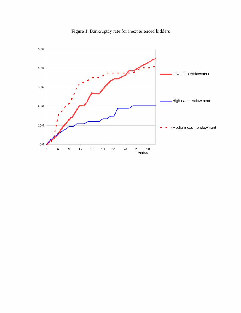
Figure 1: Bankruptcy rate for inexperienced bidders

0%

10%

20%

30%

40%

50%

3 6 9 12 15 18 21 24 27 30Period

Low cash endowment

High cash endowment

Medium cash endowment

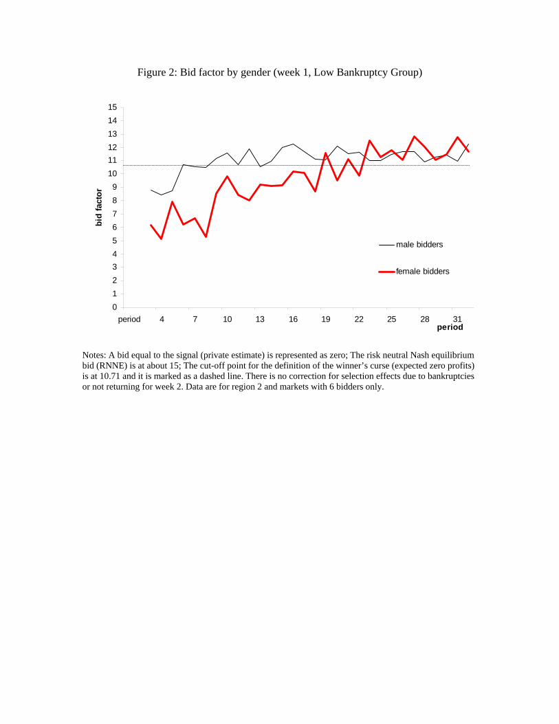
Figure 2: Bid factor by gender (week 1, Low Bankruptcy Group)

0123456789

101112131415

period 4 7 10 13 16 19 22 25 28 31

bid

fact

or

male bidders

female bidders

period

Notes: A bid equal to the signal (private estimate) is represented as zero; The risk neutral Nash equilibrium bid (RNNE) is at about 15; The cut-off point for the definition of the winner’s curse (expected zero profits) is at 10.71 and it is marked as a dashed line. There is no correction for selection effects due to bankruptcies or not returning for week 2. Data are for region 2 and markets with 6 bidders only.

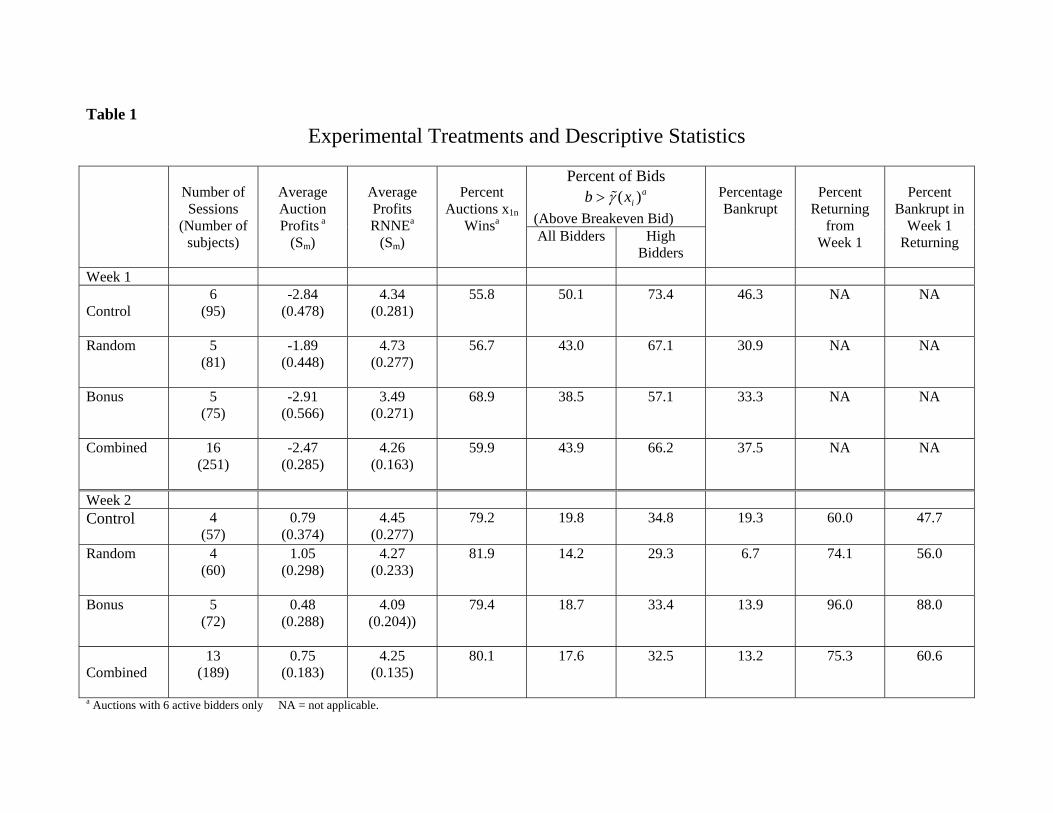
Table 1

Experimental Treatments and Descriptive Statistics

Percent of Bids ( )a ib xγ>

(Above Breakeven Bid)

Number of Sessions

(Number of subjects)

Average Auction Profits a

(Sm)

Average Profits RNNEa

(Sm)

Percent

Auctions x1n Winsa

All Bidders

High Bidders

Percentage Bankrupt

Percent

Returning from

Week 1

Percent

Bankrupt in Week 1

Returning

Week 1 Control

6 (95)

-2.84 (0.478)

4.34 (0.281)

55.8 50.1 73.4 46.3 NA NA

Random

5 (81)

-1.89 (0.448)

4.73 (0.277)

56.7 43.0 67.1 30.9 NA NA

Bonus

5 (75)

-2.91 (0.566)

3.49 (0.271)

68.9 38.5 57.1 33.3 NA NA

Combined

16 (251)

-2.47 (0.285)

4.26 (0.163)

59.9 43.9 66.2 37.5 NA NA

Week 2 Control

4 (57)

0.79 (0.374)

4.45 (0.277)

79.2 19.8 34.8 19.3 60.0 47.7

Random

4 (60)

1.05 (0.298)

4.27 (0.233)

81.9 14.2 29.3 6.7 74.1 56.0

Bonus

5 (72)

0.48 (0.288)

4.09 (0.204))

79.4 18.7 33.4 13.9 96.0 88.0

Combined

13 (189)

0.75 (0.183)

4.25 (0.135)

80.1 17.6 32.5 13.2 75.3 60.6

a Auctions with 6 active bidders only NA = not applicable.

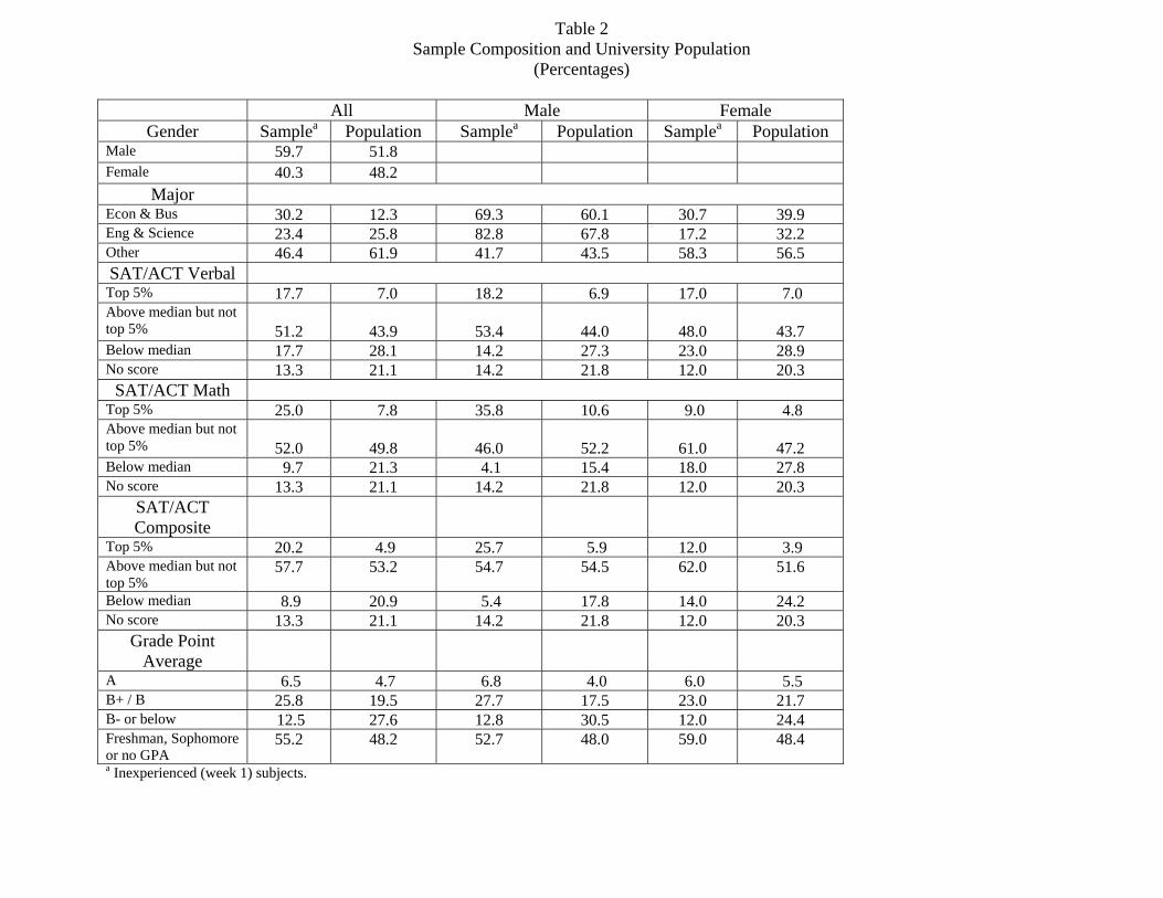
Table 2 Sample Composition and University Population

(Percentages)

All Male Female Gender Samplea Population Samplea Population Samplea Population

Male 59.7 51.8 Female 40.3 48.2

Major Econ & Bus 30.2 12.3 69.3 60.1 30.7 39.9 Eng & Science 23.4 25.8 82.8 67.8 17.2 32.2 Other 46.4 61.9 41.7 43.5 58.3 56.5 SAT/ACT Verbal

Top 5% 17.7 7.0 18.2 6.9 17.0 7.0 Above median but not top 5%

51.2

43.9

53.4

44.0

48.0

43.7

Below median 17.7 28.1 14.2 27.3 23.0 28.9 No score 13.3 21.1 14.2 21.8 12.0 20.3

SAT/ACT Math Top 5% 25.0 7.8 35.8 10.6 9.0 4.8 Above median but not top 5%

52.0

49.8

46.0

52.2

61.0

47.2

Below median 9.7 21.3 4.1 15.4 18.0 27.8 No score 13.3 21.1 14.2 21.8 12.0 20.3

SAT/ACT Composite

Top 5% 20.2 4.9 25.7 5.9 12.0 3.9 Above median but not top 5%

57.7 53.2 54.7 54.5 62.0 51.6

Below median 8.9 20.9 5.4 17.8 14.0 24.2 No score 13.3 21.1 14.2 21.8 12.0 20.3

Grade Point Average

A 6.5 4.7 6.8 4.0 6.0 5.5 B+ / B 25.8 19.5 27.7 17.5 23.0 21.7 B- or below 12.5 27.6 12.8 30.5 12.0 24.4 Freshman, Sophomore or no GPA

55.2 48.2 52.7 48.0 59.0 48.4

a Inexperienced (week 1) subjects.

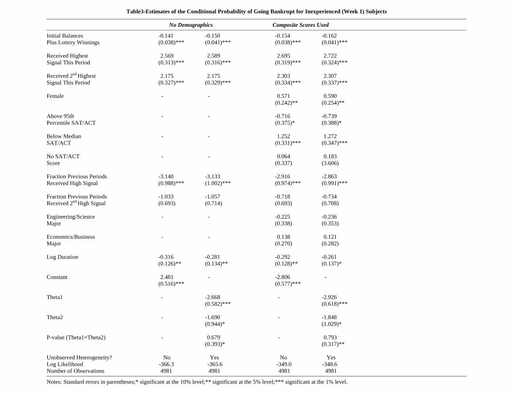
Table3-Estimates of the Conditional Probability of Going Bankrupt for Inexperienced (Week 1) Subjects

No Demographics Composite Scores Used

Initial Balances -0.141 -0.150 -0.154 -0.162 Plus Lottery Winnings (0.038)*** (0.041)*** (0.038)*** (0.041)*** Received Highest 2.569 2.589 2.695 2.722 Signal This Period (0.313)*** (0.316)*** (0.319)*** (0.324)*** Received 2nd Highest 2.175 2.175 2.303 2.307 Signal This Period (0.327)*** (0.329)*** (0.334)*** (0.337)*** Female - - 0.571 0.590

(0.242)** (0.254)** Above 95th - - -0.716 -0.739 Percentile SAT/ACT (0.375)* (0.388)* Below Median - - 1.252 1.272 SAT/ACT (0.331)*** (0.347)*** No SAT/ACT - - 0.064 0.183 Score (0.337) (3.606) Fraction Previous Periods -3.140 -3.133 -2.916 -2.863 Received High Signal (0.988)*** (1.002)*** (0.974)*** (0.991)*** Fraction Previous Periods -1.033 -1.057 -0.718 -0.734 Received 2nd High Signal (0.693) (0.714) (0.693) (0.708) Engineering/Science - - -0.225 -0.236 Major (0.338) (0.353) Economics/Business - - 0.138 0.121 Major (0.270) (0.282) Log Duration -0.316 -0.281 -0.292 -0.261

(0.126)** (0.134)** (0.128)** (0.137)* Constant 2.481 - -2.806 - (0.516)*** (0.577)*** Theta1 - -2.668 - -2.926

(0.582)*** (0.618)*** Theta2 - -1.690 - -1.848

(0.944)* (1.029)* P-value (Theta1=Theta2) - 0.679 - 0.793

(0.393)* (0.317)** Unobserved Heterogeneity? No Yes No Yes Log Likelihood -366.3 -365.6 -349.0 -348.6 Number of Observations 4981 4981 4981 4981

Notes: Standard errors in parentheses;* significant at the 10% level;** significant at the 5% level;*** significant at the 1% level.

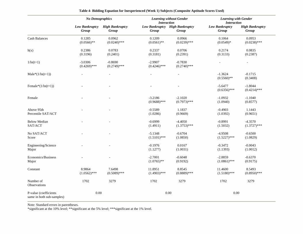
Table 4- Bidding Equation for Inexperienced (Week 1) Subjects (Composite Aptitude Scores Used)

No Demographics Learning without Gender Learning with Gender Interaction Interaction Low Bankruptcy High Bankruptcy Low Bankruptcy High Bankruptcy Low Bankruptcy High Bankruptcy Group Group Group Group Group Group

Cash Balances 0.1285 0.0962 0.1209 0.0966 0.1064 0.0953

(0.0566)** (0.0240)*** (0.0561)** (0.0239)*** (0.0549)* (0.0238)*** h(x) 0.2386 0.0783 0.2337 0.0706 0.2174 0.0835

(0.3196) (0.2401) (0.3181) (0.2391) (0.3133) (0.2387) 1/ln(t+1) -3.0306 -0.8690 -2.9907 -0.7830 - -

(0.4269)*** (0.2749)*** (0.4246)*** (0.2740)*** Male*(1/ln(t+1)) - - - - -1.3624 -0.1715

(0.5560)** (0.3408) Female*(1/ln(t+1)) - - - - -5.6477 -1.8044

(0.6356)*** (0.4214)*** Female - - -3.2186 -2.1020 -1.0932 -1.1040

(0.9688)*** (0.7973)*** (1.0940) (0.8577) Above 95th - - -0.5589 1.1837 -0.4903 1.1443 Percentile SAT/ACT (1.0286) (0.9669) (1.0392) (0.9651) Below Median - - -0.6999 -4.4050 -0.8991 -4.3570 SAT/ACT (1.4911) (1.3753)*** (1.5032) (1.3727)*** No SAT/ACT - - -5.1348 -0.6704 -4.9508 -0.6500 Score (1.5101)*** (1.0850) (1.5227)*** (1.0829) Engineering/Science - - -0.1976 0.0167 -0.3472 -0.0043 Major (1.1277) (1.0031) (1.1393) (1.0012) Economics/Business - - -2.7001 -0.6048 -2.8859 -0.6370 Major (1.0765)** (0.9192) (1.0861)*** (0.9175) Constant 8.9864 7.6498 11.8951 8.8545 11.4600 8.5493

(1.0562)*** (0.5089)*** (1.4903)*** (0.8889)*** (1.5180)*** (0.8950)*** Number of 1702 3279 1702 3279 1702 3279 Observations P-value (coefficients 0.00 0.00 0.00 same in both sub-samples)

Note: Standard errors in parentheses. *significant at the 10% level; **significant at the 5% level; ***significant at the 1% level.

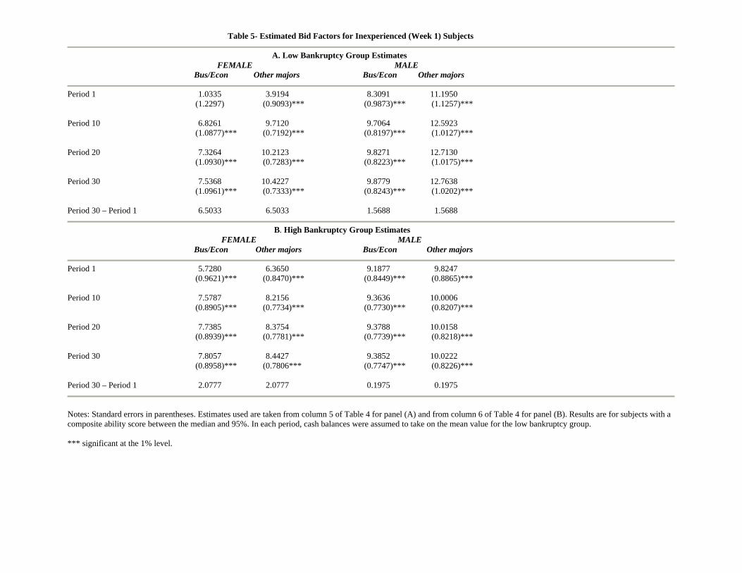
Table 5- Estimated Bid Factors for Inexperienced (Week 1) Subjects

A. Low Bankruptcy Group Estimates

FEMALE MALE Bus/Econ Other majors Bus/Econ Other majors

Period 1 1.0335 3.9194 8.3091 11.1950 (1.2297) (0.9093)*** (0.9873)*** (1.1257)*** Period 10 6.8261 9.7120 9.7064 12.5923

(1.0877)*** (0.7192)*** (0.8197)*** (1.0127)*** Period 20 7.3264 10.2123 9.8271 12.7130

(1.0930)*** (0.7283)*** (0.8223)*** (1.0175)*** Period 30 7.5368 10.4227 9.8779 12.7638

(1.0961)*** (0.7333)*** (0.8243)*** (1.0202)*** Period 30 – Period 1 6.5033 6.5033 1.5688 1.5688

B. High Bankruptcy Group Estimates FEMALE MALE Bus/Econ Other majors Bus/Econ Other majors

Period 1 5.7280 6.3650 9.1877 9.8247 (0.9621)*** (0.8470)*** (0.8449)*** (0.8865)*** Period 10 7.5787 8.2156 9.3636 10.0006 (0.8905)*** (0.7734)*** (0.7730)*** (0.8207)*** Period 20 7.7385 8.3754 9.3788 10.0158 (0.8939)*** (0.7781)*** (0.7739)*** (0.8218)*** Period 30 7.8057 8.4427 9.3852 10.0222 (0.8958)*** (0.7806*** (0.7747)*** (0.8226)*** Period 30 – Period 1 2.0777 2.0777 0.1975 0.1975

Notes: Standard errors in parentheses. Estimates used are taken from column 5 of Table 4 for panel (A) and from column 6 of Table 4 for panel (B). Results are for subjects with a composite ability score between the median and 95%. In each period, cash balances were assumed to take on the mean value for the low bankruptcy group. *** significant at the 1% level.

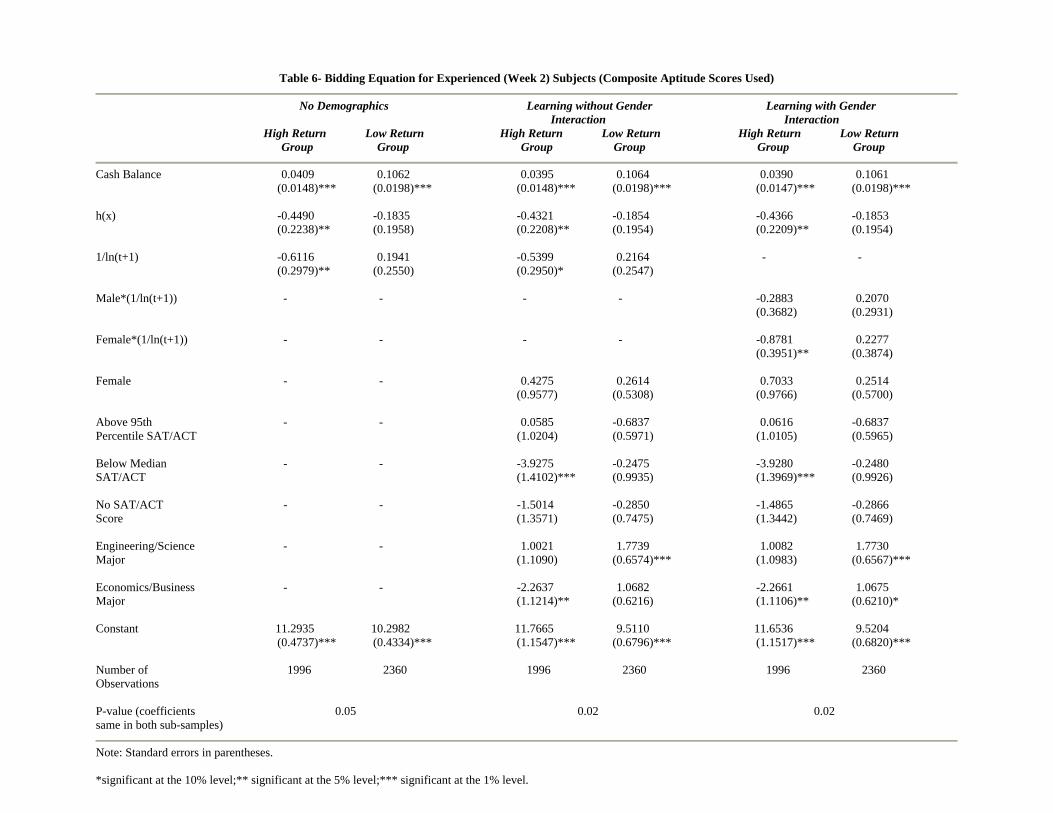
Table 6- Bidding Equation for Experienced (Week 2) Subjects (Composite Aptitude Scores Used)

No Demographics Learning without Gender Learning with Gender Interaction Interaction High Return Low Return High Return Low Return High Return Low Return Group Group Group Group Group Group

Cash Balance 0.0409 0.1062 0.0395 0.1064 0.0390 0.1061

(0.0148)*** (0.0198)*** (0.0148)*** (0.0198)*** (0.0147)*** (0.0198)*** h(x) -0.4490 -0.1835 -0.4321 -0.1854 -0.4366 -0.1853

(0.2238)** (0.1958) (0.2208)** (0.1954) (0.2209)** (0.1954) 1/ln(t+1) -0.6116 0.1941 -0.5399 0.2164 - -

(0.2979)** (0.2550) (0.2950)* (0.2547) Male*(1/ln(t+1)) - - - - -0.2883 0.2070

(0.3682) (0.2931) Female*(1/ln(t+1)) - - - - -0.8781 0.2277

(0.3951)** (0.3874) Female - - 0.4275 0.2614 0.7033 0.2514

(0.9577) (0.5308) (0.9766) (0.5700) Above 95th - - 0.0585 -0.6837 0.0616 -0.6837 Percentile SAT/ACT (1.0204) (0.5971) (1.0105) (0.5965) Below Median - - -3.9275 -0.2475 -3.9280 -0.2480 SAT/ACT (1.4102)*** (0.9935) (1.3969)*** (0.9926) No SAT/ACT - - -1.5014 -0.2850 -1.4865 -0.2866 Score (1.3571) (0.7475) (1.3442) (0.7469) Engineering/Science - - 1.0021 1.7739 1.0082 1.7730 Major (1.1090) (0.6574)*** (1.0983) (0.6567)*** Economics/Business - - -2.2637 1.0682 -2.2661 1.0675 Major (1.1214)** (0.6216) (1.1106)** (0.6210)* Constant 11.2935 10.2982 11.7665 9.5110 11.6536 9.5204

(0.4737)*** (0.4334)*** (1.1547)*** (0.6796)*** (1.1517)*** (0.6820)*** Number of 1996 2360 1996 2360 1996 2360 Observations P-value (coefficients 0.05 0.02 0.02 same in both sub-samples)

Note: Standard errors in parentheses. *significant at the 10% level;** significant at the 5% level;*** significant at the 1% level.

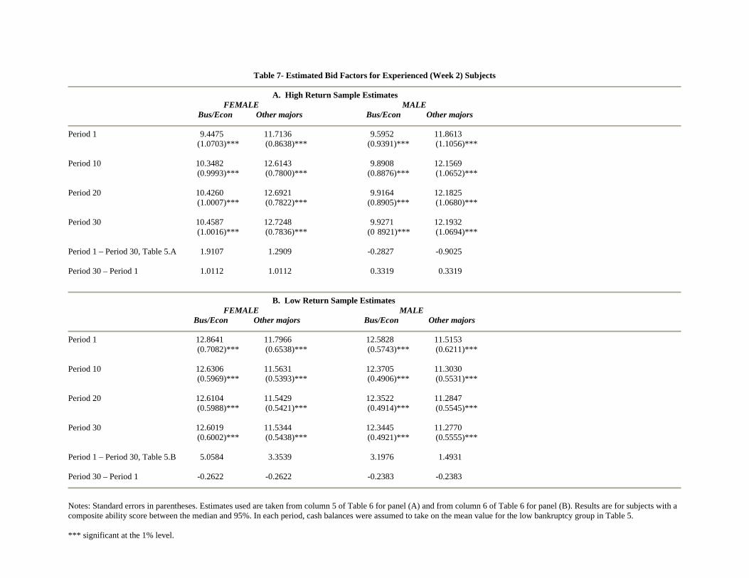
Table 7- Estimated Bid Factors for Experienced (Week 2) Subjects

A. High Return Sample Estimates FEMALE MALE Bus/Econ Other majors Bus/Econ Other majors

Period 1 9.4475 11.7136 9.5952 11.8613 (1.0703)*** (0.8638)*** (0.9391)*** (1.1056)*** Period 10 10.3482 12.6143 9.8908 12.1569 (0.9993)*** (0.7800)*** (0.8876)*** (1.0652)*** Period 20 10.4260 12.6921 9.9164 12.1825 (1.0007)*** (0.7822)*** (0.8905)*** (1.0680)*** Period 30 10.4587 12.7248 9.9271 12.1932 (1.0016)*** (0.7836)*** (0 8921)*** (1.0694)*** Period 1 – Period 30, Table 5.A 1.9107 1.2909 -0.2827 -0.9025 Period 30 – Period 1 1.0112 1.0112 0.3319 0.3319

B. Low Return Sample Estimates FEMALE MALE Bus/Econ Other majors Bus/Econ Other majors

Period 1 12.8641 11.7966 12.5828 11.5153 (0.7082)*** (0.6538)*** (0.5743)*** (0.6211)*** Period 10 12.6306 11.5631 12.3705 11.3030 (0.5969)*** (0.5393)*** (0.4906)*** (0.5531)*** Period 20 12.6104 11.5429 12.3522 11.2847 (0.5988)*** (0.5421)*** (0.4914)*** (0.5545)*** Period 30 12.6019 11.5344 12.3445 11.2770

(0.6002)*** (0.5438)*** (0.4921)*** (0.5555)***

Period 1 – Period 30, Table 5.B 5.0584 3.3539 3.1976 1.4931 Period 30 – Period 1 -0.2622 -0.2622 -0.2383 -0.2383

Notes: Standard errors in parentheses. Estimates used are taken from column 5 of Table 6 for panel (A) and from column 6 of Table 6 for panel (B). Results are for subjects with a composite ability score between the median and 95%. In each period, cash balances were assumed to take on the mean value for the low bankruptcy group in Table 5. *** significant at the 1% level.